NBER WORKING PAPER SERIES CONSUMER DEMAND UNDER PRICE UNCERTAINTY: EMPIRICAL EVIDENCE FROM THE MARKET FOR CIGARETTES Mark Coppejans Donna Gilleskie Holger Sieg Koleman Strumpf Working Paper 12156 http://www.nber.org/papers/w12156 NATIONAL BUREAU OF ECONOMIC RESEARCH 1050 Massachusetts Avenue Cambridge, MA 02138 April 2006 The views expressed herein are those of the author(s) and do not necessarily reflect the views of the National Bureau of Economic Research. ©2006 by Mark Coppejans, Donna Gilleskie, Holger Sieg and Koleman Strumpf. All rights reserved. Short sections of text, not to exceed two paragraphs, may be quoted without explicit permission provided that full credit, including © notice, is given to the source.

Welcome message from author
This document is posted to help you gain knowledge. Please leave a comment to let me know what you think about it! Share it to your friends and learn new things together.
Transcript

NBER WORKING PAPER SERIES
CONSUMER DEMAND UNDER PRICE UNCERTAINTY: EMPIRICAL EVIDENCE FROM THE MARKET FOR CIGARETTES
Mark CoppejansDonna Gilleskie
Holger SiegKoleman Strumpf
Working Paper 12156http://www.nber.org/papers/w12156
NATIONAL BUREAU OF ECONOMIC RESEARCH1050 Massachusetts Avenue
Cambridge, MA 02138April 2006
The views expressed herein are those of the author(s) and do not necessarily reflect the views of the NationalBureau of Economic Research.
©2006 by Mark Coppejans, Donna Gilleskie, Holger Sieg and Koleman Strumpf. All rights reserved. Shortsections of text, not to exceed two paragraphs, may be quoted without explicit permission provided that fullcredit, including © notice, is given to the source.

Consumer Demand under Price Uncertainty: Empirical Evidence from the Market for CigarettesMark Coppejans, Donna Gilleskie, Holger Sieg and Koleman StrumpfNBER Working Paper No. 12156April 2006JEL No. C8, D8, I1
ABSTRACT
The goal of this paper is to analyze consumer demand in markets with large price uncertainty. Wedevelop a demand model for goods that are subject to habit formation. We show that consumptionplans of forward looking individuals depend not only on preferences and current period prices, butalso on individual beliefs about the evolution of future prices. Moreover, a mean preserving spreadin the price distribution and, hence, an increase in price uncertainty reduces consumption along theoptimal path. With smoking as our application, we test the predictions of our model. We use aunique data set of prices for cigarettes collected by the Bureau of Labor Statistics to characterizeprice uncertainty and price expectations of individuals. We have also obtained access to the restricteduse version of the National Education Longitudinal Study, which provides detailed information onsmoking behavior of teenagers in the U.S. Our estimation results suggest that teenagers who live inmetropolitan areas with a large amount of cigarette price volatility have, on average, significantlylower levels of cigarette consumption. Moreover, these individuals are less likely to start consumingcigarettes. Our results also provide evidence that young individuals are forward looking. Myopicindividuals would not respond to an increase in uncertainty about future prices by reducingconsumption.
Mark CoppejansBarclays Global Investors45 Fremont StreetSan Francisco, CA [email protected]
Donna GilleskieDepartment of EconomicsUniversity of North Carolina, Chapel HillCB #3305, 6B Gardner HallChapel Hill, NC 27599-3305and [email protected]
Holger SiegTepper School of BusinessCarnegie Mellon University5000 Forbes AvenuePittsburgh, PA 15213-3890and [email protected]
Koleman StrumpfUniversity of Kansas School of BusinessSummerfield Hall1300 Sunnyside AvenueLawrence, KS [email protected]

1 Introduction
The goal of this paper is to analyze consumer demand in markets with large price
uncertainty. Our analysis differs from most previous consumer demand studies which
either assume that individuals face little uncertainty about future prices or that un-
certainty about future prices has a negligible impact on demand. While this may be a
plausible assumption in many applications, there are clearly cases in which expecta-
tions and uncertainty about future prices cannot be ignored. In these circumstances
consumer demand will be affected by price uncertainty.1 In this paper, we develop
a demand model for goods that are subject to habit formation. We show that con-
sumption plans of forward looking individuals depend not only on preferences and
current period prices, but also on individual beliefs about the evolution of future
prices. Moreover, a mean preserving spread in the price distribution and, hence, an
increase in price uncertainty reduces smoking along the optimal path.
One purpose of this paper is to quantify the effects of price uncertainty on con-
sumer demand in volatile markets. Our application focuses on the demand for
cigarettes. Our empirical analysis draws on a number of different data sets. We
1The seminal paper on market equilibrium under price uncertainty is Muth (1961). Some influen-tial recent studies are Wolak and Kolstad (1991) who study input demand under price uncertainty,Appelbaum and Ullah (1997) who analyze production decisions under price uncertainty, and Hall andRust (2002) and Osborne (2004) who consider inventory decisions under price uncertainty. There isalso an emerging literature in marketing that looks at issues related to price uncertainty. A recentapplication is Erdem, Imai, and Keane (2003) who estimate a model of brand choice under priceuncertainty.
1

use a unique price data set provided by the Bureau of Labor Statistics (BLS). The
main advantages of this data set are two-fold. We can analyze prices on the metropoli-
tan area level. Our analysis thus avoids aggregation bias inherent in data at the state
or federal level. Moreover, prices are sampled on a monthly basis, that allows us to
focus on price variation within short time periods. Our empirical findings suggest that
there is much price variation among the set of metropolitan areas analyzed in this
study. Furthermore, estimates based on aggregate time series often underestimate
the amount of price volatility experienced at the local level.
To estimate the effects of price uncertainty on consumption decisions, we need to
characterize price expectations and construct measures of price volatility. First, we
focus on historical volatility.2 These measures are relevant if individuals form adaptive
price expectations (i.e., if individuals infer future prices by looking at price realizations
in the preceding periods.) Second, we compute more sophisticated measures of price
expectations. These measures capture the idea that individuals must forecast future
price realizations. Ideally forecasts should be based on the true data generating
process (Muth, 1961). We explore regime switching models proposed by Hamilton
(1989, 1990) to model the time series properties of prices.3 Our empirical findings
suggest that for the majority of metropolitan areas studied in this paper, there are
2This approach of measuring price volatility is in the spirit of the adaptive expectation hypothesiswhich is typically attributed to Nerlove (1958).
3As an alternative to regime switching models we also consider GARCH (1,1) models (Bollerslev,1986).
2

two distinctly different regimes of price changes. There are time periods which are
fairly stable and exhibit only small changes in prices. These periods are followed by
short periods which are much more volatile and exhibit large swings in prices. In
these periods, predicted confidence intervals for future prices are quite large.
We then investigate whether the demand for cigarettes is affected by price volatil-
ity. We focus on the behavior of young individuals who may be most susceptible to
large swings in prices because their disposable income is relatively low compared to
adults. This part of the analysis is based on a restricted-use version of the National
Education Longitudinal Study (NELS) which is collected by the National Center for
Educational Statistics (NCES). We merge the NELS with BLS data on prices and
prices volatilities using geographic identifiers in the NELS. We then estimate de-
mand models to quantify the impact of price volatility on the demand for cigarettes
among teenagers. We find that individuals who live in metropolitan areas with a large
amount of price volatility have, on average, significantly lower levels of cigarette con-
sumption. Moreover, these individuals are less likely to start consuming cigarettes.
Models based on forecasted price volatility fit the data slightly better than models
based on historical volatility measures. However, formal non-nested hypothesis tests
often fail to distinguish between the alternatives. The results also provide some ev-
idence that young individuals are forward looking. If teenagers were myopic, price
volatility measures would have little explanatory power for observed choices. Our
3

findings suggest the opposite: teenagers respond to increased price uncertainty by
reducing their consumption.
There are three strands of the empirical literature on rational addiction that
are closely related to this study. Most prior empirical studies of the rational ad-
diction model follow Becker and Murphy (1988) and analyze first order conditions
that prices and quantities need to satisfy, given individuals’ quadratic utility func-
tions. Chaloupka (1991) and Becker, Grossman, and Murphy (1991, 1994) apply this
methodology and find that tobacco consumption typically responds to lagged, current
and future price changes as predicted by rational addiction theory.4 A second line of
research develops alternative tests of forward looking behavior focusing on behavioral
responses to changes in tax policy (Gruber and Koszegi, 2001) or health shocks (Ar-
cidiacono, Sieg, and Sloan, 2006).5 Finally, there are a number of empirical studies
that primarily focus on smoking initiation of teenagers.6
The rest of the paper is organized as follows. In section 2, we present a demand
model with habit formation and characterize the relationship between consumption
of addictive goods and price expectations. Section 3 focuses on measuring price
uncertainty. This part of the analysis is based on monthly price data collected by
the BLS. Section 4 investigates the impact of price uncertainty on the consumption
4Chaloupka and Warner (2000) provide an overview of the existing empirical literature on therational addiction model.
5See also Khwaja (2006).6Some recent examples include DeCicca, Kenkel, and Mathios (2002) and Gilleskie and Strumpf
(2005).
4

of cigarettes using a sample drawn from the NELS. Section 5 summarizes the main
findings and offers some conclusions that can be drawn from our analysis.
2 Price Uncertainty, Expectations, and Consumer
Demand
The starting point of our analysis is a consumer demand model that accounts for habit
formation and uncertainty about future prices.7 We would like to know whether price
uncertainty and subjective beliefs about future prices can have substantial effects on
the consumption of addictive goods such as cigarettes. Consider an individual who
can consume two types of goods: a good which is subject to habit formation denoted
by at and a composite private good denoted by ct. The stock characterizing habit
formation, St, evolves according to the following law of motion:
St+1 = δ St + at (1)
7Becker and Murphy (1988) develop the basic rational addiction model without uncertainty.Orphanides and Zervos (1995) consider uncertainty about addiction, but not price uncertainty.Arcidiacono et al. (2006) consider the case of uncertainty about health status and mortality.
5

where δ is the rate of depreciation of the stock. Individuals rank alternatives according
to a utility function:
Ut = u(ct, at, St) (2)
that satisfies standard regularity assumptions imposed in the habit formation
literature.8 Individuals are forward looking. The relevant planning horizon of an
individual is T periods. Individuals maximize expected intertemporal utility:
E
(T∑t=1
βt−1 u(ct, at, St)
)(3)
where β is the discount factor.9 Thus if β = 0, individuals are myopic. If β > 0
individuals are forward looking. Individuals face a sequence of budget constraints
given by:
ct + pt at = yt (4)
where pt is the gross-of-tax price of a at time t and yt denotes income at time t. We
have conveniently normalized the price of the composite private good to be equal
8These assumptions are smoothness, concavity, complementarity of a and S, and negativity.9Alternatively, one could assume that individuals engage in hyperbolic discounting as suggested
by Harris and Laibson (2001) and Gruber and Koszegi (2001) or make systematic mistakes as inBernheim and Rangel (2004). Our main argument rests on the notion that individuals are forwardlooking. Whether individuals adopt time-consistent or inconsistent plans is not important for ouranalysis.
6

to one.10 Prices for the addictive good evolve according to a stochastic law of mo-
tion. Individuals do not have perfect foresight. Instead, they have subjective beliefs
characterizing the distribution of future prices. Price expectations are given by the
transition density, f(pt+1 |pt).
Since we abstract from saving decisions, we can simplify the decision problem of
the individuals and substitute the budget constraint into the utility function. Define
w(yt, pt, at, St) = u(yt − ptat, at, St). (5)
Under the assumptions made above, we can express the dynamic optimization prob-
lem faced by a forward looking individual using the following recursive representation:
Vt(yt, St, pt) = maxat∈[0,yt/pt]
w(yt, pt, at, St) (6)
+β∫Vt+1(yt+1, δSt + at, , pt+1) f(pt+1|pt) dpt+1
where Vt(·) denotes the value function at time t. The state variables are yt, St, and
pt. The decision variable is at.
10For simplicity, we assume that there is no savings. This is a reasonable assumption for youngindividuals. Our analysis also largely abstracts from stockpiling which is an interesting aspect ofconsumer behavior of frequently consumed goods as discussed, for example, by Hendel and Nevo(2002). However, teenagers are less likely to have such sophisticated behavioral patterns. First, it isharder for teenagers to store large amounts of cigarettes, especially if their parents do not want themto smoke. Second, they are less likely to make bulk purchases (largely because of cash constraintsor legal issues in dealing with stores).
7

We are primarily interested in characterizing the relationship between the con-
sumption of the addictive good at and the beliefs that individuals hold about future
prices. To get more precise results, it is useful to impose more structure on the
problem. Following Orphanides and Zervos (1995) we assume that the preferences of
individuals can be characterized by the following function:
u(ct, at, St) = ln(ct) + ln(at) + Sψt (−φ+ γ at) (7)
where ψ, γ and φ are parameters of the model.11 Given this additional assumption,
we can prove the following result:
Proposition 1 Under the assumptions made above, a mean preserving spread in the
price distribution for each period will reduce smoking along the optimal path.
Broadly speaking, risk averse individuals are concerned not only about the level but
also the variance of future prices. An increase in the variance of future prices implies
an increase in the variance of future consumption. As a consequence individuals will
substitute from the risky consumption good that is subject to price uncertainty to
the consumption good without price uncertainty. More formally proposition 1 follows
from the fact that the value function is concave in prices. A rigorous proof is provided
11The utility function used above does not explicitly account for adjustment costs of the typediscussed in Suranovic, Goldfarb, and Leonard (1999). These types of adjustment costs may beimportant to explain why addicted individuals are often not satisfied with their current state ofaffairs. The analysis of this paper could be extended to incorporate adjustment costs withoutchanging the main theoretical properties of the model.
8

in Appendix A.
In summary, we have shown that the demand for goods that are subject to habit
formation depends on beliefs about future prices. Our model suggests the following
three hypotheses that can be tested empirically:
1. Myopic and forward looking individuals will reduce consumption of the addictive
good in response to a current period price increase.
2. Myopic individuals are not concerned about future prices. In particular, their
behavior does not depend on future price expectations.
3. Forward looking individuals are concerned about future prices. An increase in
the variance of future prices will decrease the current period consumption of
the addictive good.
In the remaining sections of this study, we provide an empirical investigation of these
hypotheses.
3 Measuring Price Uncertainty
3.1 Data
The focus of this paper is to analyze whether consumer decisions are affected by price
uncertainty in markets that exhibit large fluctuations in prices. Our application fo-
9
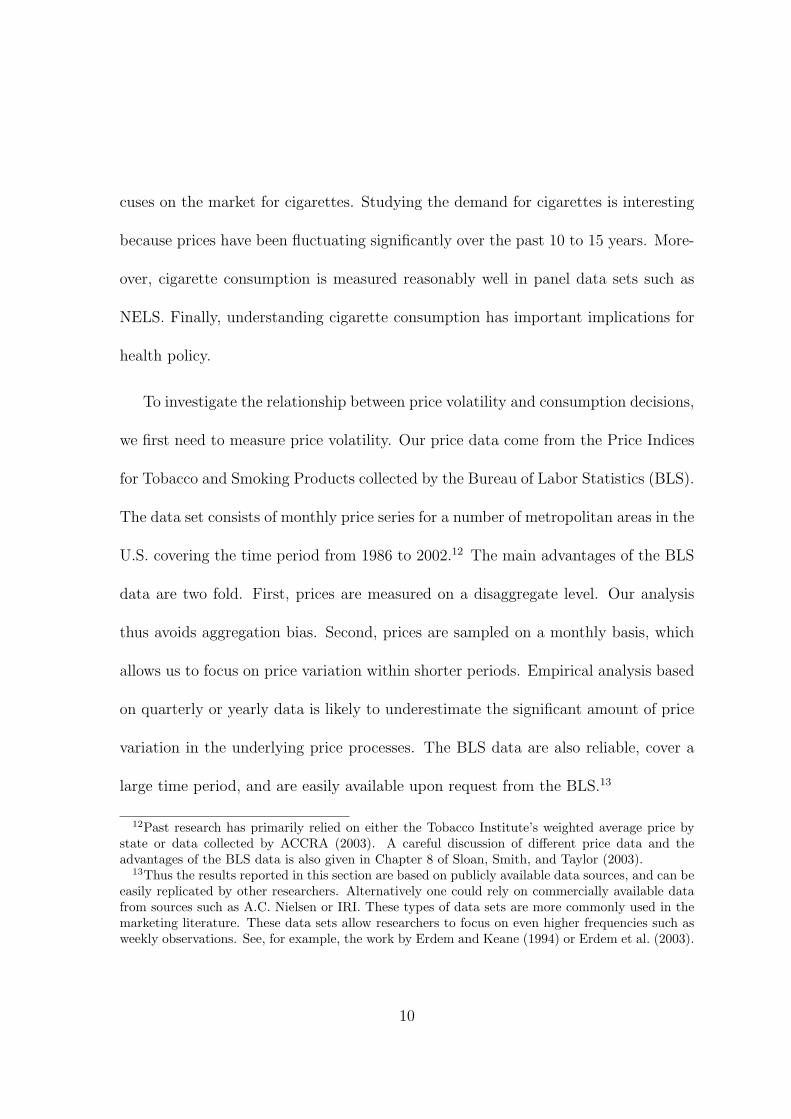
cuses on the market for cigarettes. Studying the demand for cigarettes is interesting
because prices have been fluctuating significantly over the past 10 to 15 years. More-
over, cigarette consumption is measured reasonably well in panel data sets such as
NELS. Finally, understanding cigarette consumption has important implications for
health policy.
To investigate the relationship between price volatility and consumption decisions,
we first need to measure price volatility. Our price data come from the Price Indices
for Tobacco and Smoking Products collected by the Bureau of Labor Statistics (BLS).
The data set consists of monthly price series for a number of metropolitan areas in the
U.S. covering the time period from 1986 to 2002.12 The main advantages of the BLS
data are two fold. First, prices are measured on a disaggregate level. Our analysis
thus avoids aggregation bias. Second, prices are sampled on a monthly basis, which
allows us to focus on price variation within shorter periods. Empirical analysis based
on quarterly or yearly data is likely to underestimate the significant amount of price
variation in the underlying price processes. The BLS data are also reliable, cover a
large time period, and are easily available upon request from the BLS.13
12Past research has primarily relied on either the Tobacco Institute’s weighted average price bystate or data collected by ACCRA (2003). A careful discussion of different price data and theadvantages of the BLS data is also given in Chapter 8 of Sloan, Smith, and Taylor (2003).
13Thus the results reported in this section are based on publicly available data sources, and can beeasily replicated by other researchers. Alternatively one could rely on commercially available datafrom sources such as A.C. Nielsen or IRI. These types of data sets are more commonly used in themarketing literature. These data sets allow researchers to focus on even higher frequencies such asweekly observations. See, for example, the work by Erdem and Keane (1994) or Erdem et al. (2003).
10

The BLS sample contains price indices for a large number of metropolitan areas
in the U.S. In this part of the analysis, we restrict attention to 27 metropolitan areas.
This subsample is chosen to reflect the geographical diversity within the United States.
The BLS data is an index that we converted into price per carton using the ACCRA
(2003) data which includes quarterly prices, inclusive of all excise taxes, for a carton
of cigarettes. For each metro area, we normalize the BLS index so that February 1993
is unity and then multiply by the ACCRA price from the first quarter of 1993. The
1993 match point was selected since it is the middle of the observation period and it
is in a relatively low volatility period. (The price series does not markedly change if
other dates are used.)
Table 1 reports descriptive statistics for the 27 metro areas in our sample. It re-
ports means, standard deviations, minimums and maximums for price levels over the
16 year period from 1986:12 to 2002:11. The reported minimum typically occurred
during the beginning of the time period; the maximum, towards the end. We, there-
fore, find that prices increased on average by approximately 100 percent during the
observation period.
To illustrate the basic properties of our price data, we also provide plots for
four metro areas in our sample. Figure 1 suggests that prices of tobacco products
increased substantially throughout the time period in the four metropolitan areas.
However, there are also time periods in the sample in which prices of tobacco products
11
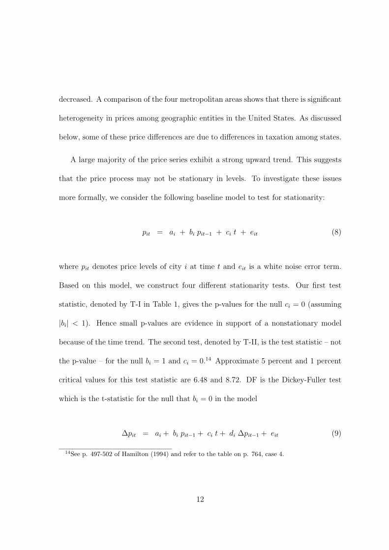
decreased. A comparison of the four metropolitan areas shows that there is significant
heterogeneity in prices among geographic entities in the United States. As discussed
below, some of these price differences are due to differences in taxation among states.
A large majority of the price series exhibit a strong upward trend. This suggests
that the price process may not be stationary in levels. To investigate these issues
more formally, we consider the following baseline model to test for stationarity:
pit = ai + bi pit−1 + ci t + eit (8)
where pit denotes price levels of city i at time t and eit is a white noise error term.
Based on this model, we construct four different stationarity tests. Our first test
statistic, denoted by T-I in Table 1, gives the p-values for the null ci = 0 (assuming
|bi| < 1). Hence small p-values are evidence in support of a nonstationary model
because of the time trend. The second test, denoted by T-II, is the test statistic – not
the p-value – for the null bi = 1 and ci = 0.14 Approximate 5 percent and 1 percent
critical values for this test statistic are 6.48 and 8.72. DF is the Dickey-Fuller test
which is the t-statistic for the null that bi = 0 in the model
∆pit = ai + bi pit−1 + ci t+ di ∆pit−1 + eit (9)
14See p. 497-502 of Hamilton (1994) and refer to the table on p. 764, case 4.
12

where ∆pit = pit − pit−1. The 95 % confidence interval for this test statistic is
(−3.69,−0.62). Finally, we report the modified Dickey Fuller (MDF) test statistic
for the null that bi = 0 and ci = 0 in the above model.
Table 1 reports the results for the four stationarity tests. Our findings suggest
that prices may not be stationary in levels. The p-values for the first test statistic
are low, and the second test statistic is often above the critical levels at commonly
used significance levels. The two versions of the DF test show similar results.
It is also interesting to ask the question whether a subset of the metropolitan areas
are driven by common stochastic trends. This may be helpful to explain some of the
short term and long term interactions of the time series. To investigate these issues
we perform a panel data unit root test suggested by Levin and Lin (1993). This test
is based on the model specification:
∆pit = ai + at + bi pit−1 +ki∑j=1
dij∆pit−j + eit. (10)
The null hypothesis is the joint hypothesis that bi = 0 for all i. Since the asymptotic
distribution of the test statistic is hard to approximate, we follow Cecchetti, Nelson,
and Sonora (2002) and use bootstrap techniques to compute the p-value associated
with the test statistic. We implement the test focusing on a subsample of our data
set which consists of the four cities used in Figure 1. We find that the p-value for the
LL test is 0.30 which is not strong evidence against our modeling approach.
13

We therefore difference the data and run the same tests on the differenced data.
Our results suggest that first differencing the data yields stationary time series. We
conclude that it is reasonable to model prices in first differences as a stationary time
series. We therefore estimate all formal pricing models reported in the next subsection
in first differences. To illustrate the main properties of the data in first differences, we
plot the time series for four metro areas in Figure 2. The plots suggest that there are
time periods that are characterized by large volatilities in prices. The last few years
in our sample are very good examples of these high volatility time periods. At the
same time there appear to be periods with fairly low variation in prices. For example,
price changes are much smaller in the middle of our observation period.
Some of the differences in estimates for the cities in our sample may be attributed
to the sampling period. For example, it is possible that we would get different esti-
mates and hence different predictions of the price volatilities if we began or ended the
price series at different points of times. Lagged price changes lead to initial condition
problems in estimation and thus affect forecasting. However, our data set is relatively
large including monthly observations for about 16 years. We expect that the type
of initial condition problems discussed above are important in shorter data sets with
yearly or quarterly observations.15
15We observe prices in the BLS data set for a much longer time period than we observe smokingchoices in the NELS. Thus our analysis of smoking behavior reported in Section 4 of this paper doesnot require us to forecast price volatilities at the beginning or the end of BLS sample period.
14

To investigate these issues more rigorously, we analyze whether large metropolitan
areas lead smaller metropolitan areas in pricing behavior. In particular, we use the
price series for New York, Chicago, and Los Angeles and investigate whether lagged
values of these series have any explanatory power in the price process of smaller metro
areas in their vicinities. We estimate the following model:
∆pit = ai + bi ∆pit−1 + ci ∆pNY,t−1 + di ∆pChi,t−1 + ei ∆pLA,t−1 + eit (11)
We calculate an F-test for the null hypothesis that ci = di = ei = 0 for the 24 cities
that are not NY, Chicago, or LA. We find that the null hypothesis is rejected for 15
out the 24 cities at 5 %. But we can only reject the null at 1% three times. We then
pick the major city which mostly influences a minor city (via significance of F-test)
and estimate the following model:
∆pit = ai + bi ∆pit−1 + ci ∆pNY,Chi,orLA,t−1 + eit (12)
We test the null hypothesis that ci = 0. Our evidence suggests that New York seems
to have some influence on other Northeastern cities such as Philadelphia, Boston,
Pittsburgh, or Detroit. The results for all other cities are inconclusive. Sometimes
we obtain counterintuitive negative point estimates. We thus conclude that there is
only limited evidence which suggests that there exists spillover effects between larger
15

and smaller cities.
Some of the price variation observed in our sample is a direct result of changes
in state and federal tax policies that were implemented during the past decade. In
1983, the federal excise tax was doubled from $0.08 per pack to $0.16 per pack. This
rate held for a decade, when the federal rate was increased another $0.08 to $0.24
per pack. In 1997, legislation passed increasing the federal tax on cigarettes to $0.34
per pack in 2000 and $0.39 per pack in 2002. Some of the cross-sectional variation of
prices is due to differences in state tax policies. Table 2 summarizes the main features
of policies during the last decade for the states in our sample. It highlights the cross
sectional and time series variation in tax rates. While all states had low rates in
1987, most doubled or tripled the tax in a series of changes over the next fifteen
years. And while many tobacco producing states maintained low rates, there were
sharp increases in other initially low tax states like California. The data, therefore,
indicate that individuals in our sample of metro areas face a wide range of market
conditions.
3.2 Expected Price Volatility
The theoretical model studied in Section 2 suggests that consumption decisions can
depend on beliefs that individuals hold about future prices. We construct two mea-
sures to characterize expected price volatility. The first measure is based on historical
16

volatility. For that we consider the price variation in the preceding periods. This mea-
sure is consistent if individual have adaptive expectations. However, individuals may
be more rational and recognize that they need to forecast future price realizations
and that extrapolating historical realizations may not be the best way to do that. To
forecast prices, it is desirable to use a formal time series model of the price process.
If individuals have correct expectations, beliefs will be based on objective price tran-
sitions; these can be estimated by an econometrician. To formulate measures char-
acterizing expectations about future price uncertainty, we estimate regime switching
models pioneered by Hamilton (1989, 1990). We consider a first-order autoregressive
regime switching model that can be written as:
∆pt = µst + ρst ∆pt−1 + εst (13)
where st is the (unobserved) state of the time series process at time t. In a regime
switching model the parameters of the autoregressive process, µst and ρst , and the
distribution of the error terms depend on the state of the process. This feature of
the model allows us to capture the fact that prices are stable in some periods and
highly volatile in other periods. We assume that εst is i.i.d. N(0, σ2s). For notational
simplicity, let us write the density of ∆pt conditional on st = j and ∆pt−1 as
f(∆pt |st = j,∆pt−1; θ) (14)
17

where θ is the parameter vector to be estimated.
The evolution of the state of the process is modelled as the outcome of an un-
observed J-state Markov chain. For simplicity let us consider a two-regime model
(J = 2). The Markov transition matrix for a two-regime model is given by:
Q =
q11 q21
q12 q22
(15)
where qij = Prst = i | st−1 = j. Denote the history of price changes up to time t-1
as ∆~pt−1. The probability that the process is in state st = j conditional on ∆~pt−1 is
written as Prst = j |∆~pt−1; θ. Given that we observe a realization ∆pt, we draw
inference about the state of the process by iterating the following two equations:
Prst = i |∆~pt; θ =f(∆pt |st = i,∆pt−1; θ) Prst = i |∆~pt−1; θ∑2j=1 f(∆pt |st = j,∆pt−1; θ) Prst = j |∆~pt−1; θ
(16)
and
Prst+1 = 1 |∆~pt; θ
Prst+1 = 2 |∆~pt; θ
=
q11 q21
q12 q22
Prst = 1 |∆~pt; θ
Prst = 2 |∆~pt; θ
(17)
Equations (16) and (17) completely characterize the stochastic evolution of the state
of the process. We have a sample of price changes observed over a sequence of T
18

periods. The likelihood function for the data is given by the following equation:
L =T∏t=1
J∑j=1
Prst = j |∆~pt−1; θ f(∆pt |st = j,∆pt−1; θ). (18)
The likelihood function does not have a closed-form analytical solution, but needs
to be computed using an Expectation-Maximization (EM) algorithm. In the EM
algorithm, we start with an initial guess for the probabilities of each state and then
iterate forward using equations (16) and (17) to compute the conditional probabilities
characterizing each state at time t.16
We estimate the regime switching models for each of the 27 metro areas. Table 3
reports the point estimates of the parameters of the different regime switching models.
Estimated standard errors are reported in parentheses. Table 3 suggests that there
is substantial heterogeneity among the metropolitan areas in our data set as the
parameter estimates differ considerably among the 27 metro areas. The estimates
for the means, µj, are typically positive in both regimes. They are often significantly
different from zero. This result reflects the earlier observation that prices were mostly
increasing during the observation period. We also find that the point estimates for
ρs are often negative in both regimes. This result suggests that there is some mean
reversion in the data. A period of positive price changes is likely to be followed by a
period with negative price changes.
16For a detailed discussion of the EM algorithm see, for example, Hamilton (1994).
19

Table 3 shows that two-state regime switching models fit the data better than
simple AR(1) specifications, at least for a large number of metro areas. The point
estimates suggest that regime 1 is characterized by large changes in prices accom-
panied with large volatility. These are the periods of price wars or changes in tax
or regulatory policies. Regime 2, in contrast, is fairly stable and shows only modest
amounts of volatility and price changes.
We have also conducted a formal test to distinguish between one-state and two-
state regime switching models for a subset of the metro areas in the data set. De-
termining the number of states in a regime switching model is, however, complicated
because standard regularity assumptions imposed in likelihood ratio tests are not met
(Hansen, 1992). One of the problems encountered here is that the null hypothesis
involves a restriction on the boundary. For these types of test there are no gen-
eral asymptotic results available. We therefore rely on bootstrapping algorithms to
construct p-values for these tests. Our findings indicate that for the majority of
metropolitan areas in our samples we can reject the null hypothesis that there is only
one state in the regime switching model.17
Regime switching models are not the only reasonable time series models that can
17We also estimated AR models with more than one lag and found that the AR(1) specificationis sufficient to capture the main regularities in the data. We have no a priori reasons to believe thata two-state regime switching model provides the best fit to the data. We performed a number ofsensitivity tests to investigate whether adding an additional state to our model would change themain empirical results. All of these tests suggested that adding a third regime to the model doesnot improve the fit of the model.
20

be fit to the data. As an additional robustness check, we follow Bollerslev (1986) and
consider GARCH(1,1) models that are given by the following equations:
∆pt = µ+ ρ∆pt−1 + εt (19)
εt ∼ N(0, σ2t ) where σ2
t = γ0 + γ1ε2t−1 + γ2σ
2t−1 (20)
We estimate a separate GARCH for each city. The parameter estimates are presented
in Table 4. As with the switching model, we find that there tends to be mean
reversion in the differenced prices (ρ < 0). The reversion terms are also comparable
in magnitude and have a similar ranking across cities as those in Table 3 from the
switching model.
Notice that the conditional variance parameters are sometimes negative (γ1 < 0,
γ2 < 0) or have a sum exceeding unity (γ1 + γ2 > 1). The latter is particularly
important in our case, since it implies that the process is not covariance stationary –
shocks do not damp out. Since GARCH models need not have a concave likelihood,
we consider a variety of maximization algorithms and continue to find these parameter
estimates. Unfortunately, this is a common feature with GARCH models. We thus
conclude that the regime switching models seem to perform slightly better in our
application than GARCH models.
21

4 Price Volatility and Demand
4.1 Data
Despite a great interest in the U.S. in understanding youth smoking behavior, few
nationally representative data sets are available that chronicle the behavior of the
same children over multiple periods of time. The National Education Longitudinal
Study of 1988 (NELS) is one exception. NELS, a continuing study sponsored by the
U.S. Department of Education’s National Center for Education Statistics, began in
1988 with the specific purpose of collecting information on educational, vocational,
and personal development of a nationally representative sample of 8th graders as
they transition from middle school into high school, through high school, and into
postsecondary institutions and the work force. Approximately 24,500 8th graders in
more than 1,000 public and private schools in all 50 states participated in the first
wave of the study. In addition to the student questionnaires, supplementary ques-
tionnaires were administered to the students’ parents, teachers, and school principals
and provide a wealth of information on the early social and academic environment
of the students. Through special agreement with the U.S. Department of Education,
we obtained access to restricted-use NELS data that include geographic information.
The first follow-up, administered in the spring of 1990, includes responses from
approximately 17,500 of the students from the 1988 base year interview, while the
22

second follow-up, administered in the spring of 1992, includes approximately 16,500
students from the original cohort. One of the many unique features of the NELS data
is that youth who leave high school prior to graduation continue to be interviewed
throughout the longitudinal study and are asked the same questions pertaining to
smoking behavior. It is therefore possible to examine the smoking behavior of all
youth, including those not represented in other national school-based surveys such as
Monitoring the Future. The NELS data contain information on the student’s back-
ground, upbringing, early family environment, early school environment, and other
behaviors. It provides many variables that have been found to be significant risk
factors for smoking such as school performance, religious affiliation, family structure
and living arrangement, and parental education. Since parents are surveyed in the
base year and second follow-up, it is possible to obtain time-varying information on
family background and socioeconomic characteristics that the student would not be
as informed about. In the first and second follow-up, school principals and teachers
continue to be surveyed, making it possible to control for important school environ-
mental characteristics as well.
We model the behavior of youths who are observed in each year (1988, 1990, and
1992) of the survey; we do not model attrition from the full sample. We keep only
those youths who were on grade during the sample period or who were permanent
dropouts (12,954 youths). We are forced to drop 2237 youths for whom smoking
23

behavior is unobserved. Because prices differ by state, another 270 are dropped if we
cannot identify the state in which they live or go to school, 196 are dropped if they
do not reside in the same state in all three waves, and 18 are deleted since important
variables are missing. We finally omit individuals who do not live in one of the cities
for which we have detailed price data. This leaves a sample consisting of 11,146
person-year observations.
Information on smoking behavior is collected in each wave of the survey. In each
year, youths are asked, ”How many cigarettes do you currently smoke in a day?”
Responses are limited to the following categories: do not smoke, smoke less than one
cigarette a day, smoke one to five cigarettes, smoke about a half pack (6-10), smoke
more than half a pack but less than two packs (11-39), and smoke two packs or more
(40+).
In general, adolescent smokers are older white youths with lower test scores and
socioeconomic status than non-smokers. They are more likely to have older siblings,
to have siblings who dropped out of school, to have one parent absent from the home,
and to report no religion.
The top panel of Table 5 shows the rapid increase in smoking participation between
1988 and 1992. Among the 935 youth observed smoking at some point in the sample,
only 16% began in 1988 while 45% started in 1990 and 39% started in 1992. The
dramatic increase in smoking rates is not surprising given that smoking initiation
24

typically occurs during the late teens. We also form indicators of the quantity smoked
conditional on being a smoker. There are no clear trends in conditional use in table
5.
Table 5 also shows that participation behavior is relatively persistent. The middle
panel shows that over 85% of individuals continue with their most recent behavior
in 1990 and 1992. Among non-smokers, this repeat behavior rate exceeds 95%. The
bottom panel shows that only an eighth of non-smokers begin smoking in either 1990
or 1992. Alternatively, the percentage of smokers who continue smoking rises by ten
percentage points between 1990 and 1992.
4.2 Empirical Evidence
Our objective is to investigate whether cigarette demand is sensitive to price levels and
price volatility. One hypothesis is that individuals are less likely to start smoking, and
to consume fewer cigarettes if they already smoke, when prices are highly volatile. As
we have seen in section 2, theory predicts that greater price variation or higher prices
make smoking less attractive for forward looking and risk averse individuals. To
investigate these hypotheses, we separately estimate logit probabilities of cigarette
smoking participation, Cox proportional hazard models of smoking initiation, and
multinomial logit probabilities of total smoking consumption (smoking intensity is
reported as a categorical variable in NELS). For each specification we are interested in
25

how cigarette price levels and volatility influence smoking behavior.18 The equations
we consider are,
Yit = β0 + β1 × Pit + β2 × Et[StdDev(Pit+1)] + γ′Xit + eit (21)
where Yit is a measure of smoking behavior for individual i in period t, Pit is the
cigarette price he faces, Et[StdDev(Pit+1)] is the expected next period price volatility,
and Xit are additional covariates. With larger Yit indicating more smoking, one
null hypothesis is that β1 < 0: individuals reduce smoking if prices increase. The
second null hypothesis is that β2 < 0: individuals smoke less if they face more price
uncertainty.19
The dependent variables, Yit, are a smoking indicator for participation logit mod-
els; first time smoking for Cox proportional hazards, and four smoking categories
(with non-smoking the omitted category) for the total consumption multinomial log-
its. The individual covariates, Xit, are gender, race, age, previous smoking status,
standardized test scores, religion, dropout indicator, sibling dropout indicator, family
composition, family socioeconomic status, parents’ education, income, and employ-
ment status, guardian’s age, and school characteristics.20
18An interesting extension of our analysis would look at smoking and drinking decisions jointly.Decker and Schwartz (2000) provide some evidence that higher alcohol prices decrease both alcoholconsumption and smoking participation suggesting a complementarity in consumption.
19We also reestimated the models using the expected future price instead of the current periodprice and found no significant differences in the parameter estimates.
20An alternative empirical framework which nests both discrete and continuous choice aspects is
26

Table 6 presents estimates of the parameters of demand models using historical
volatility measures. We use the standard deviation of monthly cigarette prices over
24 months prior to the individual’s survey date as the measure of price volatility.
This presumes individuals have adaptive expectations about prices, and the two year
window is used since this is the typical period between interviews. Our estimates are
broadly consistent with the two main hypotheses. The first two columns show that
higher prices and price volatility reduce smoking participation. The only drawback
is that the estimated coefficients of the price volatility measures have large standard
errors once we allow for observed covariates.
The last three rows in these columns report the estimates that imply economically
important effects. The fitted value Y is the proportion that smoke in the participation
specifications, the relative hazard in the Cox hazards, and the proportion smoking
in the listed category in total smoking. The fitted values reflect predictions using
observed covariates (and the full set of parameter estimates) and then forcing the
price standard deviation to the max or min in the data. Even after including a
wide range of individual characteristics (column two), a shift from the minimum
to maximum price volatility in the data would reduce smoking participation by 1.7
percentage points. This is nearly a ten percent reduction from the mean observed
smoking rate.
given, for example, by Gupta (1988) who uses a multinomial logit model of brand choice, and acumulative logit model of purchase quantity.
27

The hazard estimates in the third and fourth columns show that both price lev-
els and volatility reduce smoking take-up. To gauge the importance of the volatility
effect, the last three rows report relative hazards implied by the parameters. Af-
ter controlling for individual characteristics (column four), an increase in the price
standard deviation from the minimum to maximum would reduce the relative hazard
by 4.4 percentage points or seventeen percent of the relative hazard at the mean.
The remaining six columns show that higher prices and price volatility reduce total
cigarette consumption. The multinomial logits suggest that price variation markedly
reduces heavy smoking intensity – smoking more than half a pack per day – and shifts
individuals into the omitted non-smoking category. The last three rows again show
these effects are large even when including individual covariates.21
Table 7 reports estimates for the same demand models studied in Table 6. Here
we use forecasted volatilities based on regime switching models instead of historical
volatility measures. In general, we find that the main results of this study are robust to
different measurements of price volatility. Estimates of the main effects are significant
even after we control for observed covariates and fixed effects. We view this finding
as strong evidence supporting our main hypothesis that even young individuals are
forward looking and respond to increased price uncertainty by reducing consumption
as predicted by our theoretical model.
21The results reported in Table 6 may be subject to omitted variable problems. Any metro levelvariables that we have excluded from the analysis or are not measured precisely and are correlatedwith price volatilities would bias the results.
28

To distinguish between models based on forecasted volatility and those using his-
torical volatility, we perform a series of non-nested tests of model selection comparing
the specifications that use historical and forecasted price volatility. The model fit and
test statistics are:
• McFadden (1974) pseudo-R2 ≡ 1− LLM
LL0where LLM and LL0 are the log likeli-
hood from the full model and that using just a constant. Higher values indicate
a better model fit.
• Akaike’s information criterion (AIC) ≡ −2LLM+2pN
where p is the number of
parameters and N is the sample size. Smaller values indicate a better model
fit.
• Bayesian information criterion (BIC) ≡ −2LLM−(N−p) ln(N). Smaller values
indicate a better model fit. There is strong support that specification A is a
better fit than specification B if BICA −BICB < −7.
• Vuong (1989) likelihood ratio test statistic≡ LLA−LLB√Nω
where ω2 is an estimate of
variance of the likelihood ratio (this is a simplified form of the test statistic, since
we always compare specifications with the same degrees of freedom). Under
the null hypothesis that the models are equivalent, the Vuong statistic has
a standard normal distribution; under the null that model A (B) is better,
the statistic converges to positive (negative) infinity. The significance of the
29

test statistic can be calculated as 2Φ(Vuong), since it has a limiting normal
distribution.
Table 8 shows that the specifications using forecasted price volatilities outperform
those using historical price volatilities. The BIC statistics provide strong support in
favor of the forecasted model. The Vuong test gives more tentative support, since
the statistics are not statistically significant. Still, the statistic is negative in all cases
which provides some weak support in favor of the forecasted model.
As a final robustness check, we use the parameter estimates of the GARCH models
in Table 4 to form price volatility measures. Presuming the process is stationary, the
volatilities have an analytical solution,
V ar(pt+s|Ωt) ≡ V ar(s∑i=0
∆pt+i + pt−1|Ωt) (22)
=s∑i=0
i∑j=0
(ρs−j)2
((γ1 + γ2)
j(σ2t −
γ0
1− γ1 − γ2
) +γ0
1− γ1 − γ2
).
Price standard deviations are calculated using this formula along with the parameter
estimates from Table 4. The GARCH price volatilities are then used to explain
individual smoking behavior using the NELS data, as in Tables 6 and 7. When we
eliminate cities with implausible parameter estimates (γ1 < 0, γ2 < 0; γ1 + γ2 1),
we find that price volatility reduces smoking participation and intensity. Table 9
presents the parameter estimates, and the fitted behavior at the bottom of the table
30

indicates the volatility effect is economically significant.
5 Conclusions
In this paper we focus on the demand for goods that are subject to habit formation
or addiction in the presence of price uncertainty. Our theoretical model predicts
that forward looking individuals form beliefs about the distribution of prices in the
future. Moreover, individual consumption plans depend crucially on beliefs they hold
about future prices. To test the main implications of this model, we have assembled
a unique data set to analyze the market for cigarettes. Our empirical findings suggest
that consumers face considerable uncertainty about future market conditions. Prices
and market conditions also vary significantly among the set of metropolitan areas
analyzed in this study. The variation in price uncertainty across space and time thus
allows us to test whether individuals respond to price uncertainty as predicted by our
theoretical model.
We have constructed two types of measures of expected price variability: one based
on adaptive expectations using historical volatilities and another based on forecasted
price volatility using regime switching and GARCH models. We have estimated
reduced form models of cigarette consumption that are based on the restricted use
version of NELS that allows us to match individuals to metropolitan areas. The
empirical evidence confirms the main predictions of our model. We find that teenagers
31

who live in metropolitan areas with large amounts of price volatility have, on average,
significantly lower levels of cigarette consumption than individuals in low volatility
areas. Models based on forecasted price volatility fit the data better than models
based on historical volatility measures. We thus conclude that young individuals are
forward looking and respond to changes in price uncertainty.
Understanding the role that uncertainty and risk aversion play in determining
consumption decisions of addictive goods has important policy implications. Indi-
viduals often face significant uncertainty about future tax policies. This uncertainty
about future taxes is likely to affect consumer choices. Moreover, federal and state
governments sometimes try to change behavior by announcing policies that may be
implemented in the future. Our findings suggest that these policy announcements
may be effective if they permanently change the beliefs that individuals hold about
future prices. If, on the other hand, an announced tax increase is perceived to be
temporary or if individuals believe that it is not likely to be implemented, then it
will have, at best, modest effects on individual consumption. Tax policies thus not
only affect prices in the period that they are announced or enacted, but they also af-
fect beliefs about future prices. Announced policy changes can have large immediate
effects if they are perceived to be credible.22
Our analysis provides ample scope for future research. Our findings illustrate the
22Gruber and Koszegi (2001) provide some empirical evidence in favor of this hypothesis.
32

need to control for price expectations and uncertainty in empirical demand analysis.
These findings, thus, raise a number of questions regarding the common practice
of ignoring uncertainty about future prices in demand analysis or assuming perfect
foresight about prices. Our estimates of the pricing processes reflect the observed
equilibria in the regional markets. From the perspective of consumers that is all that
matters. It is, however, an interesting question to ask what supply side models would
yield price processes that are similar to the ones we observe in the data. Future
research should help us understand how supply side conditions interact with demand
models of the type considered in this paper to generate equilibria that not only exhibit
large price fluctuations across time but also the large degree of spatial price dispersion.
33

Acknowledgments
We would like to thank Tim Bollerslev, Martin Gaynor, Bruce Hansen, Carolyn
Levine, Frank Sloan, and V. Kerry Smith for comments and suggestions. We also
thank Derek Brown and Justin Trogden for research assistance. The data used in
this paper were provided by the Bureau of Labor Statistics and by the Department
of Education. We would like to thank Bill Cook, Roger von Haefen, Pat Jackman,
David Johnson, and Lois Orr at the BLS. Financial support was provided by grants
from the NIH-NIAAA (R01 AA12162-01) and the National Advisory Child and Hu-
man Development Council (1R01 HD42256-01). The opinions expressed here do not
necessarily reflect those of Barclays Global Investors.
34

A Proof of Proposition 1
We prove the result in two steps.
Result 1 A mean preserving spread in the price distribution for a single period will
reduce smoking along the optimal path under the functional forms used in the main
analysis.
Proof: Suppose prices in a single period t = s are stochastic. Let ps follow the
density f(ps|σ) where σ characterizes the dispersion. The path of all other variables
is known with certainty. We continue to assume that period utility follows equation
(7), the budget constraint follows (4), and the addiction stock satisfies the law of
motion in (1). An individual’s optimization problem is
maxa,c
∫ T∑t
βt−1(ln(ct) + ln(at) + Sψt (φ+ γat)
)f(ps|σ)dps
s.t. St+1 = δSt + at (23)
ct = yt − ptat
St, St−1, . . ., yt∀t, pt∀t 6=s ∈ Ωt
where Ωt is the information set at time t (we specify below when σ ∈ Ωt).
After substituting in the constraints and optimizing over the smoking choices we
have the first order conditions,
35

∫ (−pt
yt − ptat+
1
at+ γSψt + βWt(at)
)f(ps|σ)dps = 0 ∀t (24)
where
Wt(at) ≡ ψSψ−1t+1 (φ+ γat+1) (25)
+∑r>t
βr−t−1
(−pr
yr − prar+
1
ar+ γSψr + βψSψ−1
r+1 (φ+ γar+1)
)∂ar∂at
= ψSψ−1t+1 (φ+ γat+1).
The second equality in equation (26) follows from applying the t+1 first order condi-
tion, and Wt(at) depends on at through its effect on St+1 and at+1. Along the optimal
path the second order condition must be satisfied (the value function is concave),
∂∫ ( −pt
yt−ptat+ 1
at+ γSψt + βWt(at)
)f(ps|σ)dps
∂at< 0. (26)
Finally, ct > 0 → yt − ptat > 0, which implies,
∂ −pt
yt−ptat
∂pt=
−yt(yt − ptat)2
< 0 (27)
∂2 −pt
yt−ptat
∂p2t
=−2atyt
(yt − ptat)3< 0 ↔ yt − ptat > 0.
36

This means the first order condition is concave in current prices, since pt directly
enters equation (24) only through the first term.
Now we consider the effect of a mean preserving spread in the price distribution (an
increase in σ) for the single period t = s. Suppose initially that this is unanticipated
until t = s, so optimal at ∀t<s are unaffected. The mean preserving spread reduces
the left hand side of equation (24) due to the concavity result in (27). To maintain
optimality, as (the only free variable at t = s) adjusts: as must decrease since this
will increase (24) via (26). at ∀t>s decline by an induction argument. The addiction
stock St ≡ δSt−1 + at−1 falls, since the induction assumption states at−1 declines
and so St−1 falls for t > s + 1 (Ss is unchanged). This means at declines due to
the usual adjacent complementarity argument: the complementarity and negativity
assumptions on preferences (Orphanides and Zervos, 1995) imply,
ψ, γ ≥ 0 →∂∫ ( −pt
yt−ptat+ 1
at+ γSψt + βWt(at)
)f(ps|σ)dps
∂St≥ 0. (28)
So when St decreases, equations (24), (26) and (28) require that at (the only free
variable in equation (24)) also decreases.
Now suppose that the mean preserving spread is anticipated in some period p ≤ s.
This will reduce ap following the adjacent complementarity argument above, and the
smoking level continues to decline during and after the change in σ. Combining all
37

the results,
∂at∂σ
≤ 0 ∀t≥p (29)
where p is the first period where the mean preserving spread is anticipated.
Q.E.D.
Result 2 A mean preserving spread in the price distribution for each and every period
will reduce smoking along the optimal path under the functional forms used in the main
analysis.
Proof: A proof by induction follows from repeated application of the proof of Re-
sult 1.
Q.E.D.
38

References
ACCRA (2003). ACCRA Cost of Living Index. Arlington, VA.
Appelbaum, E. and Ullah, A. (1997). Estimation of Moments and Production Decisions under
Uncertainty. Review of Economics and Statistics, 79 (4), 631–637.
Arcidiacono, P., Sieg, H., and Sloan, F. (2006). Living Rationally Under the Volcano? Heavy
Drinking and Smoking Among the Elderly. International Economic Review, forthcoming.
Becker, G., Grossman, M., and Murphy, K. (1991). Rational Addiction and the Effect of Price on
Consumption. American Economic Review, 81 (2), 237–242.
Becker, G., Grossman, M., and Murphy, K. (1994). An Empirical Analysis of Cigarette Addiction.
American Economic Review, 84 (3), 396–418.
Becker, G. and Murphy, K. (1988). A Theory of Rational Addiction. Journal of Political Economy,
96 (4), 675–700.
Bernheim, D. and Rangel, A. (2004). Addiction and Cue-Triggered Decision Processes. American
Economic Review, 94(5), 1558–1590.
Bollerslev, T. (1986). Generalized Autogressive Conditional Heteroskedasticity. Journal of Econo-
metrics, 31, 307–327.
Cecchetti, S., Nelson, M., and Sonora, R. (2002). Price Index Convergence Among United States
Cities. International Economic Review, 43, 1081–1109.
Chaloupka, F. (1991). Rational Addictive Behavior and Cigarette Smoking. Journal of Political
Economy, 99 (4), 722–742.
Chaloupka, F. and Warner, K. (2000). The Economics of Smoking. In: Handbook of Health Eco-
nomics, pp. 1151–1227. North Holland.
39

DeCicca, P., Kenkel, D., and Mathios, A. (2002). Putting Out the Fires: Will Higher Taxes Reduce
the Onset of Youth Smoking? Journal of Political Economy, 110(1), 144–69.
Decker, S. and Schwartz, A. (2000). Cigarettes and Alcohol: Substitutes or Compliments? NBER
Working Paper 7535.
Erdem, T., Imai, S., and Keane, M. (2003). Brand and Quantity Choice Dynamics Under Price
Uncertainty. Quantitative Marketing and Economics, 1, 5–64.
Erdem, T. and Keane, M. (1994). Decision Making Under Uncertainty: Capturing Choice Dynamics
in a Turbulent Consumer Market. Marketing Science, 16, 1–21.
Gilleskie, D. and Strumpf, K. (2005). The Behavioral Dynamics of Youth Smoking. Journal of
Human Resources, 40 (4), 822–866.
Gruber, J. and Koszegi, B. (2001). Is Addiction Rational: Theory and Evidence. Quarterly Journal
of Economics, 116(4), 1261–1304.
Gupta, S. (1988). Impact of Sales Promotions on When, What, and How Much To Buy. Journal of
Marketing Research, 25, 342–355.
Hall, G. and Rust, J. (2002). Econometric Models for Endogenously Sampled Time Series: The
Case of Commodity Price Speculation in the Steel Market. Working Paper.
Hamilton, J. (1989). A New Approach to the Economic Analysis of Nonstationary Time Series and
Business Cycles. Econometrica, 57, 357–384.
Hamilton, J. (1990). Analysis of Time Series Subject to Changes in Regime. Journal of Econometrics,
45, 39–70.
Hamilton, J. (1994). Time Series Analysis. Princeton University Press.
Hansen, B. (1992). The Likelihood Ratio Test Under Nonstandard Conditions: Testing the Markov
Switching Model of GNP. Journal of Applied Econometrics, 7, S61–S82.
40

Harris, C. and Laibson, D. (2001). Dynamic Choice of Hyperbolic Consumers. Econometrica, 69
(4), 935–958.
Hendel, I. and Nevo, A. (2002). Measuring the Implications of Sales and Consumer Stockpiling
Behavior. Working Paper.
Khwaja, A. (2006). Health Insurance, Habits and health Outcomes: A Dynamic Stochastic Model
of Investments in Health. Working Paper.
Levin, A. and Lin, C. (1993). Unit Root Tests in Panel Data: New Results. Working Paper, Board
of Governors of the Federal Reserve System.
McFadden, D. (1974). The Measurement of Urban Travel Demand. Journal of Public Economics,
3, 303–328.
Muth, J. (1961). Rational Expectations and the Theory of Price Movements. Econometrica, 29,
315–335.
Nerlove, M. (1958). Adaptive Expectations and Cobweb Phenomena. Quarterly Journal of Eco-
nomics, 73, 227–240.
Orphanides, A. and Zervos, D. (1995). Rational Addiction with Learning and Regret. Journal of
Political Economy, 103 (4), 739–758.
Osborne, T. (2004). Market News in Commodity Price Theory: Application to the Ethiopian Grain
Market. Review of Economic Studies, 71 (1), 133–164.
Sloan, F., Smith, V., and Taylor, D. (2003). Parsing the Smoking Puzzle: Information, Risk Per-
ception and Choice. Harvard University Press. Cambridge.
Suranovic, S., Goldfarb, B., and Leonard, T. (1999). An Economic Theory of Cigarette Addiction.
Journal of Health Economics, 18(1), 1–29.
41

Vuong, Q. (1989). Likelihood Ratio Test For Model-Selection and Non-Nested Hypotheses. Econo-
metrica, 57, 307–334.
Wolak, F. and Kolstad, C. (1991). A Model of Heterogeneous Input Demand Under Price Uncer-
tainty. American Economic Review, 81 (3), 514–38.
42
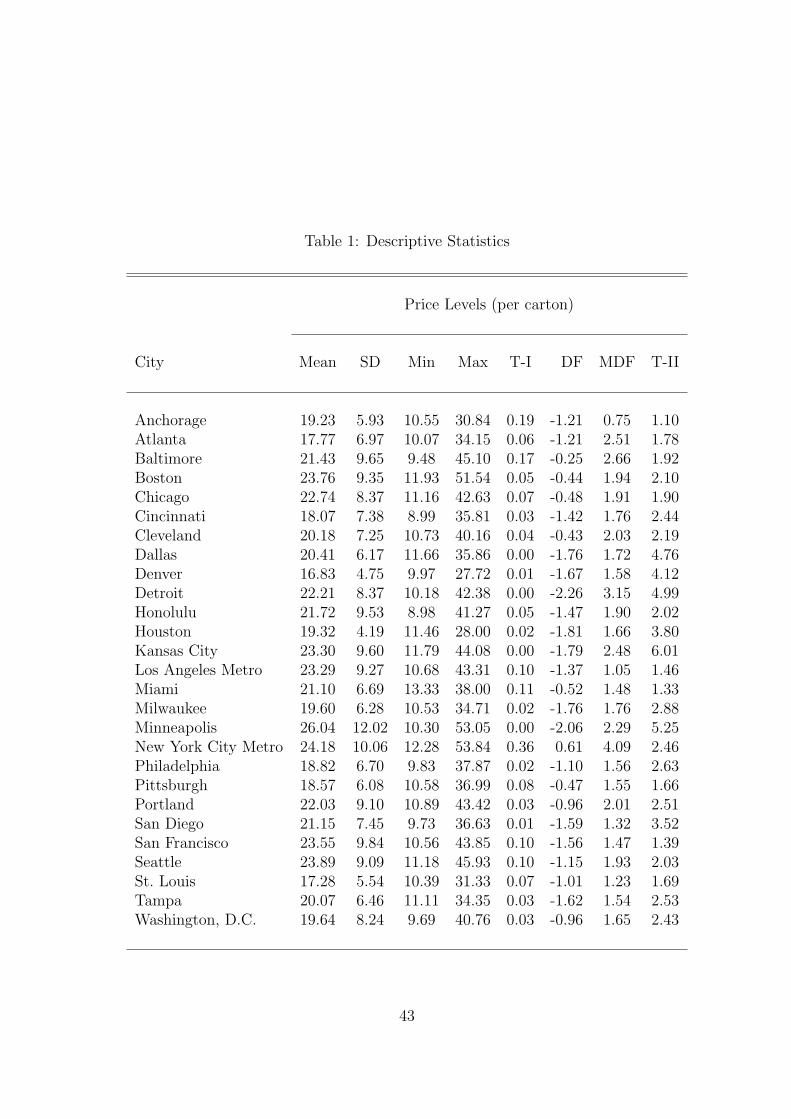
Table 1: Descriptive Statistics
Price Levels (per carton)
City Mean SD Min Max T-I DF MDF T-II
Anchorage 19.23 5.93 10.55 30.84 0.19 -1.21 0.75 1.10Atlanta 17.77 6.97 10.07 34.15 0.06 -1.21 2.51 1.78Baltimore 21.43 9.65 9.48 45.10 0.17 -0.25 2.66 1.92Boston 23.76 9.35 11.93 51.54 0.05 -0.44 1.94 2.10Chicago 22.74 8.37 11.16 42.63 0.07 -0.48 1.91 1.90Cincinnati 18.07 7.38 8.99 35.81 0.03 -1.42 1.76 2.44Cleveland 20.18 7.25 10.73 40.16 0.04 -0.43 2.03 2.19Dallas 20.41 6.17 11.66 35.86 0.00 -1.76 1.72 4.76Denver 16.83 4.75 9.97 27.72 0.01 -1.67 1.58 4.12Detroit 22.21 8.37 10.18 42.38 0.00 -2.26 3.15 4.99Honolulu 21.72 9.53 8.98 41.27 0.05 -1.47 1.90 2.02Houston 19.32 4.19 11.46 28.00 0.02 -1.81 1.66 3.80Kansas City 23.30 9.60 11.79 44.08 0.00 -1.79 2.48 6.01Los Angeles Metro 23.29 9.27 10.68 43.31 0.10 -1.37 1.05 1.46Miami 21.10 6.69 13.33 38.00 0.11 -0.52 1.48 1.33Milwaukee 19.60 6.28 10.53 34.71 0.02 -1.76 1.76 2.88Minneapolis 26.04 12.02 10.30 53.05 0.00 -2.06 2.29 5.25New York City Metro 24.18 10.06 12.28 53.84 0.36 0.61 4.09 2.46Philadelphia 18.82 6.70 9.83 37.87 0.02 -1.10 1.56 2.63Pittsburgh 18.57 6.08 10.58 36.99 0.08 -0.47 1.55 1.66Portland 22.03 9.10 10.89 43.42 0.03 -0.96 2.01 2.51San Diego 21.15 7.45 9.73 36.63 0.01 -1.59 1.32 3.52San Francisco 23.55 9.84 10.56 43.85 0.10 -1.56 1.47 1.39Seattle 23.89 9.09 11.18 45.93 0.10 -1.15 1.93 2.03St. Louis 17.28 5.54 10.39 31.33 0.07 -1.01 1.23 1.69Tampa 20.07 6.46 11.11 34.35 0.03 -1.62 1.54 2.53Washington, D.C. 19.64 8.24 9.69 40.76 0.03 -0.96 1.65 2.43
43

Table 2: Annual Cigarette Taxes (in cents per package)
1987 2002 87-02 87-02 # ofState tax tax mean std dev changes
Alaska 16 100 46.82 35.78 2California 10 87 46.35 28.74 3Colorado 15 20 19.71 1.21 1Connecticut 26 111 46.82 18.77 5Delaware 14 24 21.06 4.70 2District of Columbia 13 65 46.06 23.15 4Florida 21 33.9 30.81 4.98 2Georgia 12 12 12.00 0 0Hawaii 28 120 63.82 30.12 4Illinois 20 98 41.53 20.44 4Indiana 10.5 55.5 17.26 9.99 2Maryland 13 100 37.12 24.77 4Massachusetts 26 151 53.94 32.93 3Michigan 21 125 53.94 31.42 3Missouri 13 17 15.12 2.06 1New Jersey 25 150 51.82 32.67 4New York 21 150 57.47 35.28 5Ohio 14 55 22.88 9.08 3Oregon 27 128 47.18 27.45 5Pennsylvania 18 100 30.41 18.99 4Texas 20.5 41 35.94 8.22 2Virginia 2.5 2.5 2.50 0 0Wisconsin 25 77 43.59 16.77 5
44

Table 3: Markov-Switching Estimates
City q11 q22 µ1 µ2 ρ1 ρ2 σ21 σ2
2
Anchorage 0.676 0.600 0.195 0.000 -0.285 0.000 0.914 0.000(0.052) (0.057) (0.095) (0.006) (0.118) (0.005) (0.131) (0.012)
Atlanta 0.657 0.549 0.246 0.000 -0.416 -0.000 0.882 0.000(0.053) (0.058) (0.094) (0.006) (0.112) (0.008) (0.123) (0.013)
Baltimore 0.782 0.491 0.313 0.000 -0.249 0.000 0.805 0.000(0.053) (0.076) (0.095) (0.010) (0.099) (0.013) (0.107) (0.021)
Boston 0.920 0.943 0.421 0.127 -0.401 -0.074 3.102 0.106(0.051) (0.028) (0.232) (0.036) (0.127) (0.085) (0.559) (0.018)
Chicago 0.965 0.975 0.409 0.090 -0.470 -0.094 1.249 0.036(0.099) (0.019) (0.202) (0.021) (0.216) (0.085) (0.290) (0.007)
Cincinnati 0.699 0.415 0.234 0.000 -0.520 -0.000 1.002 0.000(0.055) (0.068) (0.097) (0.010) (0.100) (0.012) (0.136) (0.024)
Cleveland 0.904 0.936 0.323 0.124 -0.456 -0.342 1.500 0.036(0.057) (0.028) (0.155) (0.021) (0.131) (0.066) (0.276) (0.007)
Dallas 0.765 0.511 0.208 0.002 -0.529 -0.019 1.683 0.000(0.058) (0.070) (0.123) (0.012) (0.095) (0.018) (0.225) (0.063)
Denver 0.758 0.508 0.181 -0.000 -0.511 -0.000 0.965 0.000(0.046) (0.068) (0.092) (0.008) (0.059) (0.009) (0.130) (0.024)
Detroit 0.868 0.916 0.328 0.112 -0.261 -0.155 2.185 0.044(0.059) (0.032) (0.192) (0.023) (0.131) (0.062) (0.403) (0.010)
Honolulu 0.609 0.633 0.371 0.000 -0.314 -0.000 0.997 0.000(0.059) (0.054) (0.108) (0.006) (0.128) (0.007) (0.141) (0.011)
Houston 0.791 0.528 0.144 -0.000 -0.467 -0.000 0.768 0.000(0.042) (0.065) (0.081) (0.007) (0.095) (0.009) (0.093) (0.011)
Kansas City 0.894 0.964 0.459 0.079 -0.708 -0.002 4.583 0.033(0.084) (0.018) (0.394) (0.016) (0.249) (0.041) (1.163) (0.007)
Los Angeles metro 0.885 0.933 0.315 0.079 -0.224 0.066 2.861 0.053(0.060) (0.028) (0.226) (0.025) (0.130) (0.068) (0.541) (0.012)
Miami 0.685 0.711 0.338 0.048 -0.214 -0.972 1.056 0.016(0.067) (0.056) (0.117) (0.017) (0.113) (0.018) (0.166) (0.020)
Milwaukee 0.962 0.981 0.185 0.109 -0.287 -0.153 1.403 0.070(0.137) (0.050) (0.269) (0.031) (0.365) (0.094) (0.411) (0.010)
Minneapolis 0.729 0.556 0.383 0.000 -0.683 -0.000 2.727 0.000(0.047) (0.065) (0.152) (0.011) (0.097) (0.006) (0.357) (0.036)
New York metro 0.848 0.923 0.430 0.080 0.043 0.089 1.312 0.014(0.064) (0.028) (0.177) (0.012) (0.149) (0.047) (0.251) (0.005)
45
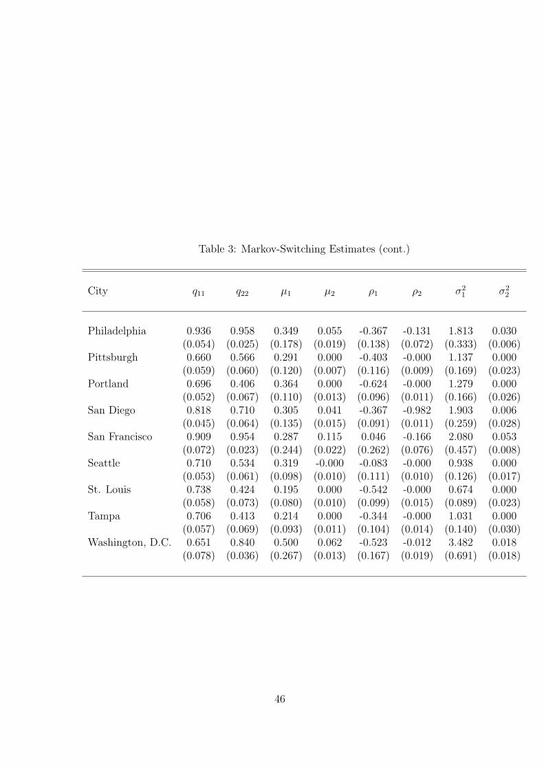
Table 3: Markov-Switching Estimates (cont.)
City q11 q22 µ1 µ2 ρ1 ρ2 σ21 σ2
2
Philadelphia 0.936 0.958 0.349 0.055 -0.367 -0.131 1.813 0.030(0.054) (0.025) (0.178) (0.019) (0.138) (0.072) (0.333) (0.006)
Pittsburgh 0.660 0.566 0.291 0.000 -0.403 -0.000 1.137 0.000(0.059) (0.060) (0.120) (0.007) (0.116) (0.009) (0.169) (0.023)
Portland 0.696 0.406 0.364 0.000 -0.624 -0.000 1.279 0.000(0.052) (0.067) (0.110) (0.013) (0.096) (0.011) (0.166) (0.026)
San Diego 0.818 0.710 0.305 0.041 -0.367 -0.982 1.903 0.006(0.045) (0.064) (0.135) (0.015) (0.091) (0.011) (0.259) (0.028)
San Francisco 0.909 0.954 0.287 0.115 0.046 -0.166 2.080 0.053(0.072) (0.023) (0.244) (0.022) (0.262) (0.076) (0.457) (0.008)
Seattle 0.710 0.534 0.319 -0.000 -0.083 -0.000 0.938 0.000(0.053) (0.061) (0.098) (0.010) (0.111) (0.010) (0.126) (0.017)
St. Louis 0.738 0.424 0.195 0.000 -0.542 -0.000 0.674 0.000(0.058) (0.073) (0.080) (0.010) (0.099) (0.015) (0.089) (0.023)
Tampa 0.706 0.413 0.214 0.000 -0.344 -0.000 1.031 0.000(0.057) (0.069) (0.093) (0.011) (0.104) (0.014) (0.140) (0.030)
Washington, D.C. 0.651 0.840 0.500 0.062 -0.523 -0.012 3.482 0.018(0.078) (0.036) (0.267) (0.013) (0.167) (0.019) (0.691) (0.018)
46
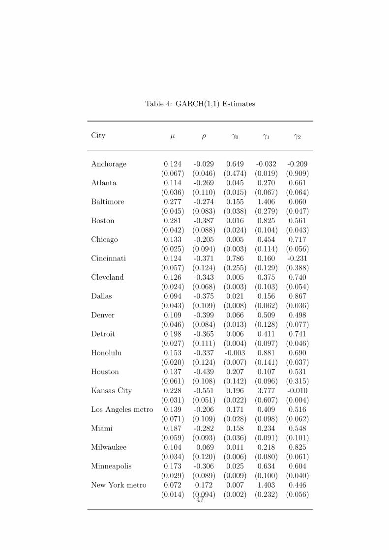
Table 4: GARCH(1,1) Estimates
City µ ρ γ0 γ1 γ2
Anchorage 0.124 -0.029 0.649 -0.032 -0.209(0.067) (0.046) (0.474) (0.019) (0.909)
Atlanta 0.114 -0.269 0.045 0.270 0.661(0.036) (0.110) (0.015) (0.067) (0.064)
Baltimore 0.277 -0.274 0.155 1.406 0.060(0.045) (0.083) (0.038) (0.279) (0.047)
Boston 0.281 -0.387 0.016 0.825 0.561(0.042) (0.088) (0.024) (0.104) (0.043)
Chicago 0.133 -0.205 0.005 0.454 0.717(0.025) (0.094) (0.003) (0.114) (0.056)
Cincinnati 0.124 -0.371 0.786 0.160 -0.231(0.057) (0.124) (0.255) (0.129) (0.388)
Cleveland 0.126 -0.343 0.005 0.375 0.740(0.024) (0.068) (0.003) (0.103) (0.054)
Dallas 0.094 -0.375 0.021 0.156 0.867(0.043) (0.109) (0.008) (0.062) (0.036)
Denver 0.109 -0.399 0.066 0.509 0.498(0.046) (0.084) (0.013) (0.128) (0.077)
Detroit 0.198 -0.365 0.006 0.411 0.741(0.027) (0.111) (0.004) (0.097) (0.046)
Honolulu 0.153 -0.337 -0.003 0.881 0.690(0.020) (0.124) (0.007) (0.141) (0.037)
Houston 0.137 -0.439 0.207 0.107 0.531(0.061) (0.108) (0.142) (0.096) (0.315)
Kansas City 0.228 -0.551 0.196 3.777 -0.010(0.031) (0.051) (0.022) (0.607) (0.004)
Los Angeles metro 0.139 -0.206 0.171 0.409 0.516(0.071) (0.109) (0.028) (0.098) (0.062)
Miami 0.187 -0.282 0.158 0.234 0.548(0.059) (0.093) (0.036) (0.091) (0.101)
Milwaukee 0.104 -0.069 0.011 0.218 0.825(0.034) (0.120) (0.006) (0.080) (0.061)
Minneapolis 0.173 -0.306 0.025 0.634 0.604(0.029) (0.089) (0.009) (0.100) (0.040)
New York metro 0.072 0.172 0.007 1.403 0.446(0.014) (0.094) (0.002) (0.232) (0.056)
47
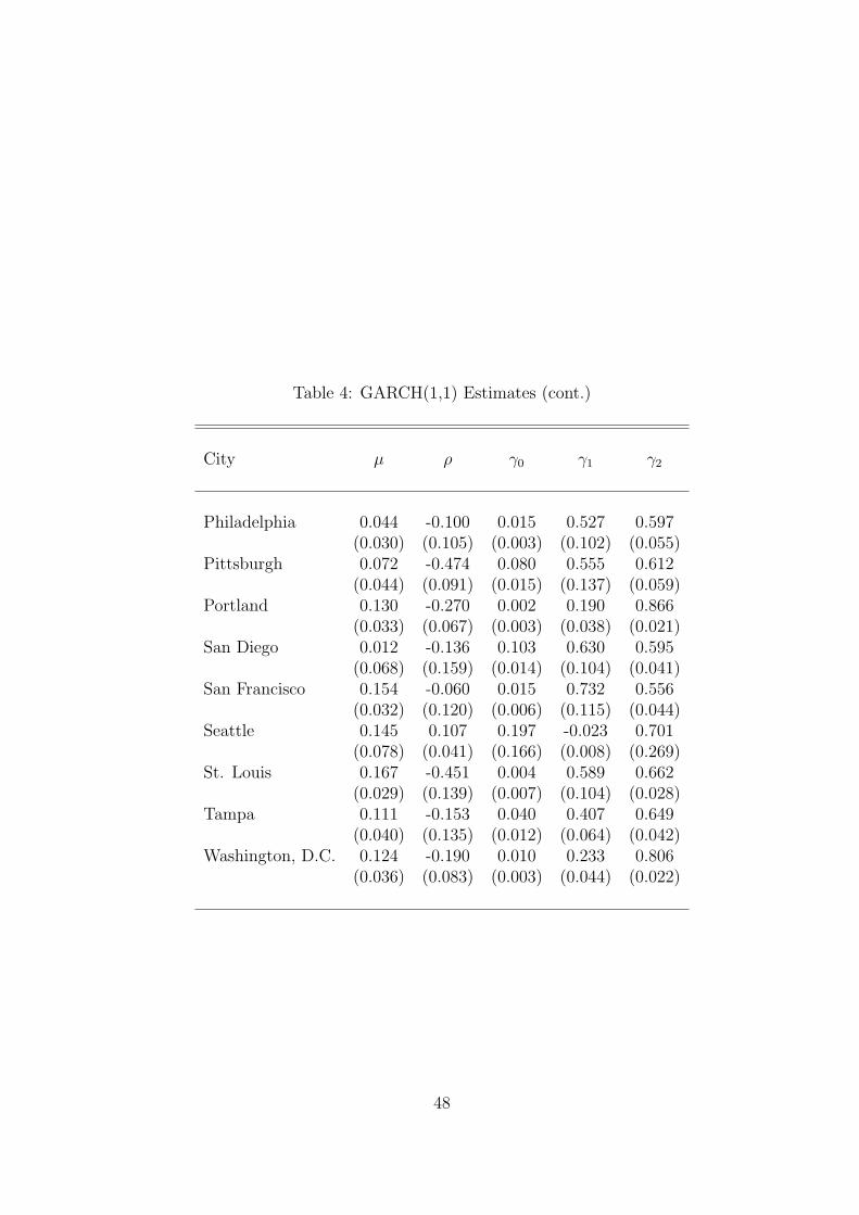
Table 4: GARCH(1,1) Estimates (cont.)
City µ ρ γ0 γ1 γ2
Philadelphia 0.044 -0.100 0.015 0.527 0.597(0.030) (0.105) (0.003) (0.102) (0.055)
Pittsburgh 0.072 -0.474 0.080 0.555 0.612(0.044) (0.091) (0.015) (0.137) (0.059)
Portland 0.130 -0.270 0.002 0.190 0.866(0.033) (0.067) (0.003) (0.038) (0.021)
San Diego 0.012 -0.136 0.103 0.630 0.595(0.068) (0.159) (0.014) (0.104) (0.041)
San Francisco 0.154 -0.060 0.015 0.732 0.556(0.032) (0.120) (0.006) (0.115) (0.044)
Seattle 0.145 0.107 0.197 -0.023 0.701(0.078) (0.041) (0.166) (0.008) (0.269)
St. Louis 0.167 -0.451 0.004 0.589 0.662(0.029) (0.139) (0.007) (0.104) (0.028)
Tampa 0.111 -0.153 0.040 0.407 0.649(0.040) (0.135) (0.012) (0.064) (0.042)
Washington, D.C. 0.124 -0.190 0.010 0.233 0.806(0.036) (0.083) (0.003) (0.044) (0.022)
48

Table 5: Smoking Dynamics in NELS
BehaviorCigarette Use (conditional on smoking)
Smoke Smoke Smoke Smokeany 1-5 cigs 6-10 cigs 11+ cigs
Full Sample 12.80 59.64 20.32 20.041988 4.03 60.93 16.56 22.521990 13.91 66.15 17.70 16.151992 20.56 54.99 22.83 22.18
PersistencePrior Behavior
Overall Non-Smoker Smoker1990 87.09 98.33 17.511992 86.27 95.58 50.26
Participation transition matrix:participation as function of prior behavior
Prior BehaviorNon-Smoker Smoker
1990 12.02 64.901992 12.01 74.51
Notes: Sample size is 11,146 person-year observations.Notes: All numbers are percentages.
49

Table 6: Estimates of Smoking Behavior from NELS: Historical Volatility Measures
(Logit) (Cox proportional hazard) (Multinomial Logit)Participation Hazard of Participation Total Consumption: cigs/day
1− 5 6− 10 > 10 1− 5 6− 10 > 10
Priceit -0.105 -0.053 -0.076 -0.048 -0.096 -0.145 -0.084 -0.052 -0.092 -0.000(0.021) (0.026) (0.025) (0.027) (0.026) (0.041) (0.042) (0.031) (0.052) (0.056)
StdDev(Priceit) -0.172 -0.053 -0.160 -0.043 -0.095 -0.107 -0.581 -0.034 0.138 -0.380(0.096) (0.110) (0.105) (0.110) (0.116) (0.204) (0.231) (0.126) (0.229) (0.265)
Year FE Yes Yes No No Yes YesIndividual Covariates No Yes No Yes No YesN 11146 11146 10437 10437 11146 11146log L -3981.28 -3315.47 -7595.68 -7478.76 -5331.13 -4417.88
Fitted ValuesY | Data 0.128 0.128 0.287 0.152 0.076 0.026 0.026 0.076 0.026 0.026Y | Min(Std Dev(Priceit)) 0.147 0.132 0.324 0.158 0.081 0.028 0.043 0.078 0.022 0.034Y | Max(Std Dev(Priceit)) 0.057 0.106 0.118 0.120 0.051 0.016 0.001 0.064 0.053 0.004
Note: Standard errors are in parentheses.
50
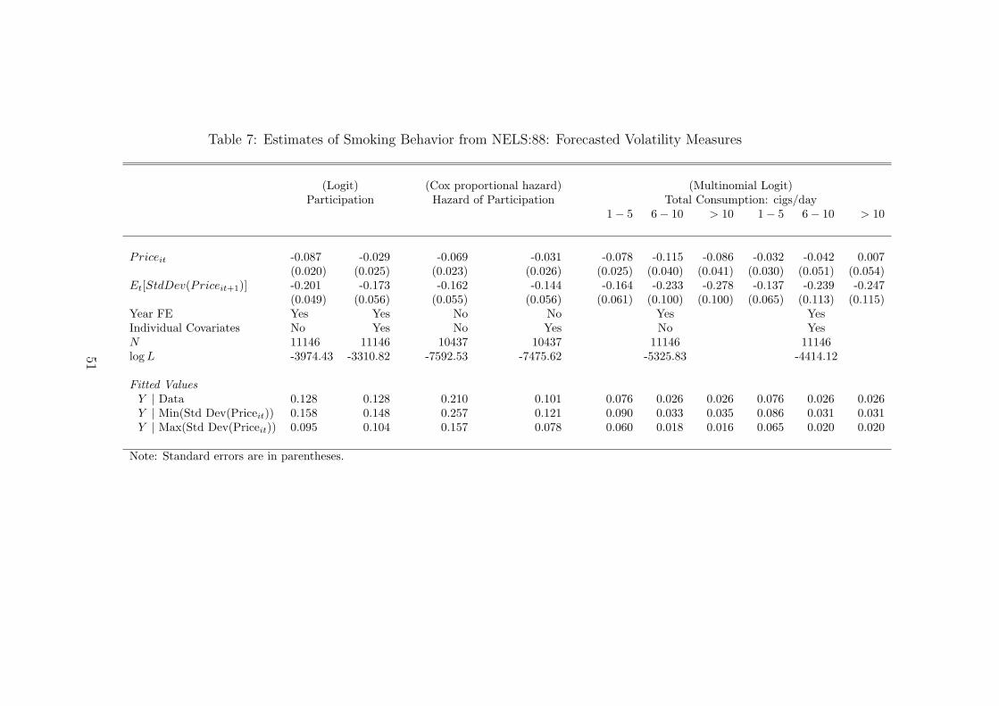
Table 7: Estimates of Smoking Behavior from NELS:88: Forecasted Volatility Measures
(Logit) (Cox proportional hazard) (Multinomial Logit)Participation Hazard of Participation Total Consumption: cigs/day
1− 5 6− 10 > 10 1− 5 6− 10 > 10
Priceit -0.087 -0.029 -0.069 -0.031 -0.078 -0.115 -0.086 -0.032 -0.042 0.007(0.020) (0.025) (0.023) (0.026) (0.025) (0.040) (0.041) (0.030) (0.051) (0.054)
Et[StdDev(Priceit+1)] -0.201 -0.173 -0.162 -0.144 -0.164 -0.233 -0.278 -0.137 -0.239 -0.247(0.049) (0.056) (0.055) (0.056) (0.061) (0.100) (0.100) (0.065) (0.113) (0.115)
Year FE Yes Yes No No Yes YesIndividual Covariates No Yes No Yes No YesN 11146 11146 10437 10437 11146 11146log L -3974.43 -3310.82 -7592.53 -7475.62 -5325.83 -4414.12
Fitted ValuesY | Data 0.128 0.128 0.210 0.101 0.076 0.026 0.026 0.076 0.026 0.026Y | Min(Std Dev(Priceit)) 0.158 0.148 0.257 0.121 0.090 0.033 0.035 0.086 0.031 0.031Y | Max(Std Dev(Priceit)) 0.095 0.104 0.157 0.078 0.060 0.018 0.016 0.065 0.020 0.020
Note: Standard errors are in parentheses.
51
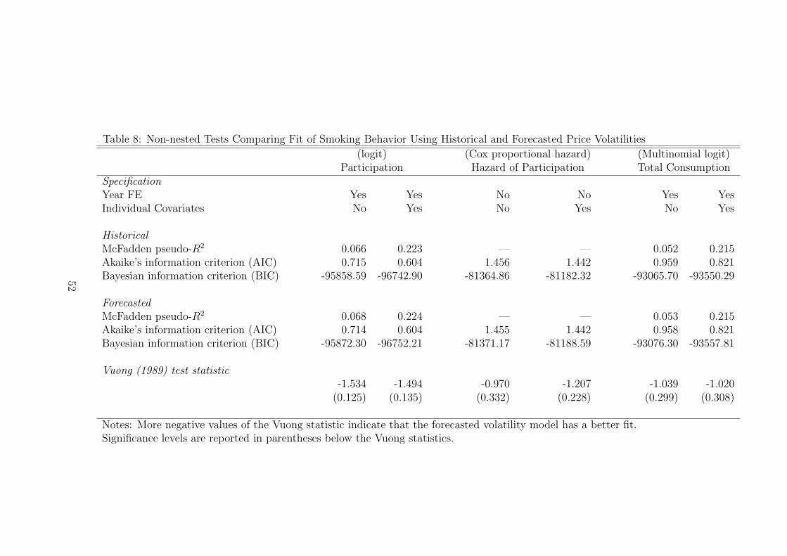
Table 8: Non-nested Tests Comparing Fit of Smoking Behavior Using Historical and Forecasted Price Volatilities
(logit) (Cox proportional hazard) (Multinomial logit)Participation Hazard of Participation Total Consumption
SpecificationYear FE Yes Yes No No Yes YesIndividual Covariates No Yes No Yes No Yes
HistoricalMcFadden pseudo-R2 0.066 0.223 — — 0.052 0.215Akaike’s information criterion (AIC) 0.715 0.604 1.456 1.442 0.959 0.821Bayesian information criterion (BIC) -95858.59 -96742.90 -81364.86 -81182.32 -93065.70 -93550.29
ForecastedMcFadden pseudo-R2 0.068 0.224 — — 0.053 0.215Akaike’s information criterion (AIC) 0.714 0.604 1.455 1.442 0.958 0.821Bayesian information criterion (BIC) -95872.30 -96752.21 -81371.17 -81188.59 -93076.30 -93557.81
Vuong (1989) test statistic-1.534 -1.494 -0.970 -1.207 -1.039 -1.020
(0.125) (0.135) (0.332) (0.228) (0.299) (0.308)
Notes: More negative values of the Vuong statistic indicate that the forecasted volatility model has a better fit.Significance levels are reported in parentheses below the Vuong statistics.
52
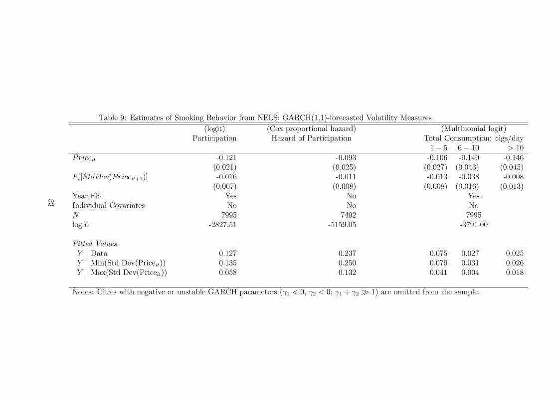
Table 9: Estimates of Smoking Behavior from NELS: GARCH(1,1)-forecasted Volatility Measures
(logit) (Cox proportional hazard) (Multinomial logit)Participation Hazard of Participation Total Consumption: cigs/day
1− 5 6− 10 > 10Priceit -0.121 -0.093 -0.106 -0.140 -0.146
(0.021) (0.025) (0.027) (0.043) (0.045)Et[StdDev(Priceit+1)] -0.016 -0.011 -0.013 -0.038 -0.008
(0.007) (0.008) (0.008) (0.016) (0.013)Year FE Yes No YesIndividual Covariates No No NoN 7995 7492 7995logL -2827.51 -5159.05 -3791.00
Fitted ValuesY | Data 0.127 0.237 0.075 0.027 0.025Y | Min(Std Dev(Priceit)) 0.135 0.250 0.079 0.031 0.026Y | Max(Std Dev(Priceit)) 0.058 0.132 0.041 0.004 0.018
Notes: Cities with negative or unstable GARCH parameters (γ1 < 0, γ2 < 0; γ1 + γ2 1) are omitted from the sample.
53

Figure 1: Prices in Levels
Houston
0
10
20
30
40
50
Los Angeles Metro
Minneapolis
1988 1992 1996 20000
10
20
30
40
50
New York Metro
1988 1992 1996 2000
54
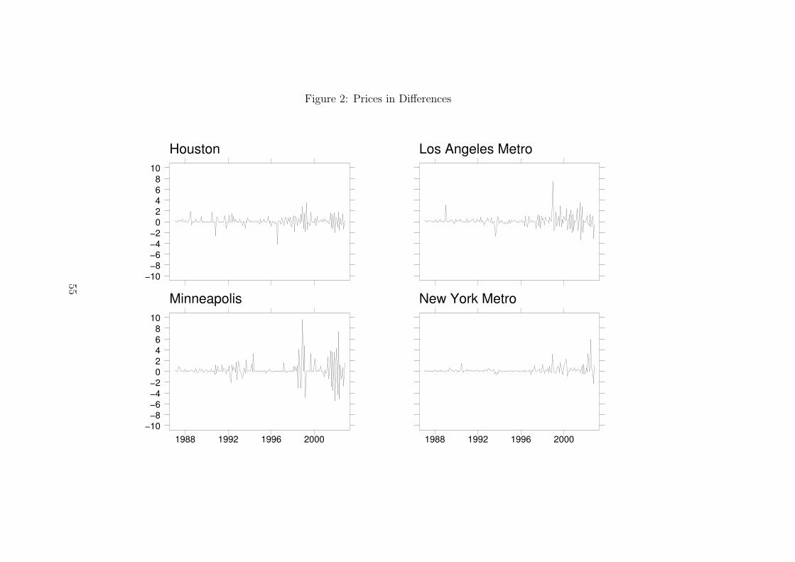
Figure 2: Prices in Differences
Houston
−10−8−6−4−2
02468
10
Los Angeles Metro
Minneapolis
1988 1992 1996 2000−10−8−6−4−2
02468
10
New York Metro
1988 1992 1996 2000
55
Related Documents


