NAVAL POSTGRADUATE SCHOOL MONTEREY, CALIFORNIA THESIS Approved for public release; distribution is unlimited DEFENSE AGAINST ROCKET ATTACKS IN THE PRESENCE OF FALSE CUES by Lior Harari December 2008 Thesis Advisor: Moshe Kress Thesis Co-Advisor: Roberto Szechtman Second Reader: Patricia Jacobs

Welcome message from author
This document is posted to help you gain knowledge. Please leave a comment to let me know what you think about it! Share it to your friends and learn new things together.
Transcript

NAVAL
POSTGRADUATE SCHOOL
MONTEREY, CALIFORNIA
THESIS
Approved for public release; distribution is unlimited
DEFENSE AGAINST ROCKET ATTACKS IN THE PRESENCE OF FALSE CUES
by
Lior Harari
December 2008
Thesis Advisor: Moshe Kress Thesis Co-Advisor: Roberto Szechtman Second Reader: Patricia Jacobs

THIS PAGE INTENTIONALLY LEFT BLANK
i
REPORT DOCUMENTATION PAGE Form Approved OMB No. 0704-0188 Public reporting burden for this collection of information is estimated to average 1 hour per response, including the time for reviewing instruction, searching existing data sources, gathering and maintaining the data needed, and completing and reviewing the collection of information. Send comments regarding this burden estimate or any other aspect of this collection of information, including suggestions for reducing this burden, to Washington headquarters Services, Directorate for Information Operations and Reports, 1215 Jefferson Davis Highway, Suite 1204, Arlington, VA 22202-4302, and to the Office of Management and Budget, Paperwork Reduction Project (0704-0188) Washington DC 20503. 1. AGENCY USE ONLY (Leave blank)
2. REPORT DATE December 2008
3. REPORT TYPE AND DATES COVERED Master’s Thesis
4. TITLE : Defense Against Rocket Attaches in the Presence of False Cues 6. AUTHOR(S) Lior Harari
5. FUNDING NUMBERS
7. PERFORMING ORGANIZATION NAME(S) AND ADDRESS(ES) Naval Postgraduate School Monterey, CA 93943-5000
8. PERFORMING ORGANIZATION REPORT NUMBER
9. SPONSORING /MONITORING AGENCY NAME(S) AND ADDRESS(ES) N/A
10. SPONSORING/MONITORING AGENCY REPORT NUMBER
11. SUPPLEMENTARY NOTES The views expressed in this thesis are those of the author and do not reflect the official policy or position of the Department of Defense or the U.S. Government. 12a. DISTRIBUTION / AVAILABILITY STATEMENT Approved for public release; distribution is unlimited
12b. DISTRIBUTION CODE
13. ABSTRACT (maximum 200 words) Rocket attacks on civilian and military targets, from both Hezbollah (South Lebanon) and Hammas (Gaza strip) have been causing a major operational problem for the Israeli Defense Forces for over two decades. In recent years U.S. forces are facing similar attacks in Afghanistan and Iraq against both remote military outposts and in the heart of Bagdad (“Green zone”). The insurgents are using mortars and short range rockets, whose launch platforms have very low signature prior to launch. The insurgents have adopted a "shoot and scoot" tactic making it hard to detect them in time to retaliate effectively. In this thesis we present a new analytic probability model, that addresses this tactical situation. The defender’s decision tradeoffs are explored and quantified. A new counter mortar/rocket tactic is suggested and explored using the probability model. An extended simulation model is developed to explore the situation when the defender is using a sensor that is subject to false positive detections.
15. NUMBER OF PAGES
99
14. SUBJECT TERMS Stochastic Model, Missile defence, Stochastic duel
16. PRICE CODE
17. SECURITY CLASSIFICATION OF REPORT
Unclassified
18. SECURITY CLASSIFICATION OF THIS PAGE
Unclassified
19. SECURITY CLASSIFICATION OF ABSTRACT
Unclassified
20. LIMITATION OF ABSTRACT
UU NSN 7540-01-280-5500 Standard Form 298 (Rev. 2-89) Prescribed by ANSI Std. 239-18

ii
THIS PAGE INTENTIONALLY LEFT BLANK
iii
Approved for public release; distribution is unlimited
DEFENSE AGAINST ROCKET ATTACKS IN THE PRESENCE OF FALSE CUES
Lior Harari
Captain, Israeli Army (IDF) B.Sc., Hebrew University of Jerusalem, 2002
Submitted in partial fulfillment of the requirements for the degree of
MASTER OF SCIENCE IN OPERATIONS RESEARCH
from the
NAVAL POSTGRADUATE SCHOOL December 2008
Author: Lior Harari
Approved by: Moshe Kress Thesis Advisor Roberto Szechtman Thesis Co-Advisor Patricia Jacobs Second Reader
James Eagle Chairman, Department of Operations Research

iv
THIS PAGE INTENTIONALLY LEFT BLANK

v
ABSTRACT
Rocket attacks on civilian and military targets, from both Hezbollah (South
Lebanon) and Hammas (Gaza strip) have been causing a major operational problem for
the Israeli Defense Forces for over two decades. In recent years, U.S. forces are facing
similar attacks in Afghanistan and Iraq against both remote military outposts and in the
heart of Bagdad (“Green zone”). The insurgents are using mortars and short range
rockets, whose launch platforms have very low signature prior to launch. The insurgents
have adopted a "shoot and scoot" tactic making it hard to detect them in time to retaliate
effectively. In this thesis we present a new analytic probability model, that addresses this
tactical situation. The defender’s decision tradeoffs are explored and quantified. A new
counter mortar/rocket tactic is suggested and explored using the probability model. An
extended simulation model is developed to explore the situation when the defender is
using a sensor that is subject to false positive detections.

vi
THIS PAGE INTENTIONALLY LEFT BLANK
vii
TABLE OF CONTENTS
I. INTRODUCTION........................................................................................................1
II. THE COMBAT SITUATION AND ENGAGEMENT TACTICS..........................3 A. CURRENT COMBAT SITUATION AND TACTICS.................................3 B. SUGGESTED TACTIC AND WEAPON......................................................4 C. SCENARIO ......................................................................................................5
III. THE ANALYTIC MODEL - NO FALSE POSITIVES DETECTIONS................7 A. GROUND SENSOR AND “DUMB” MISSILE ............................................8
1. Assumption ...........................................................................................8 2. Deriving the Model Equation..............................................................8 3. Deriving ( )N k N kH t− − .............................................................................9
3.1 First Case - Uniform Distributions ..........................................9 3.2 Second Case – Normal Distributions .....................................11 3.3 Third Case - Exponential Distributions .................................11
4. Analysis ...............................................................................................12 5. Tradeoff: Wait or Launch?...............................................................21
B. GROUND SENSOR AND “SMART” MISSILE........................................27 1. Assumptions .......................................................................................27 2. Ground Sensor Guided “Smart” Missile (Method 1) .....................28 3. Onboard Sensor “Smart” Missile (Method 2).................................36
IV. THE CASE OF FALSE POSITIVE DETECTIONS - A SIMULATION MODEL ......................................................................................................................47 A. INTRODUCING FALSE DETECTIONS ...................................................47
1. Assumptions .......................................................................................47 2. The Firing Rule ˆ ˆ( , )M T ......................................................................47 3. Problem Definition.............................................................................48
B. SIMULATION DESCRIPTION...................................................................49 1. Events Graphs ....................................................................................49 2. The Simulation Model .......................................................................50
C. ANALYSIS .....................................................................................................53 1. Positive Salvo Declaration as a Function of the Firing Rule
ˆ ˆ( , )M T ..................................................................................................53 2. False Salvo Declaration as a Function of the Firing Rule
ˆ ˆ( , )M T ..................................................................................................55 3. Results of the Base Case Scenario ....................................................57 4. The Effect of the False Detection Rate.............................................63 5. The Effect of the Missile Flight Time..............................................67 6. The Effect of the Salvos Rate ............................................................68 7. The Exponential Case ........................................................................71
V. SUMMARY ................................................................................................................75

viii
APPENDIX A.........................................................................................................................77
LIST OF REFERENCES......................................................................................................79
INITIAL DISTRIBUTION LIST .........................................................................................81
ix
LIST OF FIGURES
Figure 1. Probability of success for different missile flight times* ................................14 Figure 2. Probability of a timely hit for different missile flight times (in seconds)
and number of residual rockets* ......................................................................15 Figure 3. Probability of a timely hit for different missile flight times (in seconds)
and number of residual rockets (increased variability) *.................................18 Figure 4. Probability of success for different missile flight times (in seconds)
(increased variability) ......................................................................................19 Figure 5. Probability of a timely hit or different missile flight times (in seconds) and
number of residual rockets (Exponential case) *............................................20 Figure 6. Probability of success for different missile flight times (in seconds)
(Exponential case)............................................................................................21 Figure 7. Probability of success for different missile flight times (in seconds) and
different M values.* .........................................................................................23 Figure 8. Probability of success for different missile flight times (in seconds) and
different M values.* (Perfect detection) ..........................................................25 Figure 9. Probability of success for different missile flight times (in seconds) and
different M values.* (Exponential case) ..........................................................26 Figure 10. Simulation estimates* for the Probability of success for a ground sensor
guided “smart” missile ( 1)M = and, calculated Probability of success for the “dumb” missile launched at different number of detections (M) **..........30
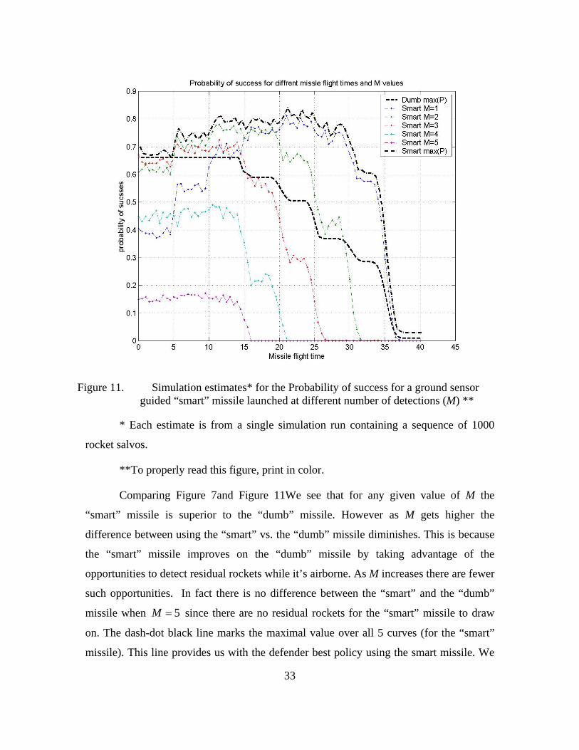
Figure 11. Simulation estimates* for the Probability of success for a ground sensor guided “smart” missile launched at different number of detections (M) ** ....33
Figure 12. Probability of success for a ground sensor guided “smart” missile and, for the “dumb” missile launched at different number of detections (M)* (Exponential case)............................................................................................35
Figure 13. Single detection probability of kill for different types of sensors ...................38 Figure 14. 38 Figure 15. Probability of rocket detection for different types of sensors..........................39 Figure 16. Simulation estimates* for the Probability of success as a function of the
missile flight time (in seconds) for different types of sensors ( 1)M = .**.......40 Figure 17. Simulation estimates* for the Probability of success as a function of the
missile flight time (in seconds) for different types of sensors ( 1)M = .** (Exponential case)............................................................................................42
Figure 18. Simulation estimates* for the Probability of success as a function of the missile flight time (in seconds) for onboard “Active sensor, for different values of M.** (Uniform case) ........................................................................43
Figure 19. Simulation estimates* for Probability of success as a function of the missile flight time (in seconds) for onboard “Passive sensor, for different values of M.* (Uniform case) ..........................................................................44
Figure 20. Simulation estimates* for the Probability of success as a function of the missile flight time for onboard “Active sensor, for different values of M.** (Exponential case) ..................................................................................45
x
Figure 21. Simulation estimates* for the Probability of success as a function of the missile flight time for onboard “Passive sensor, for different values of M.** (Exponential case) ..................................................................................46
Figure 22. Event graph example........................................................................................49 Figure 23. Simulation event graph part A .........................................................................51 Figure 24. Simulation event graph part B .........................................................................52 Figure 25. Simulation estimates* of the Probability of positive salvo declaration vs.
T̂ (in seconds) for different values of M̂ ** ...................................................54 Figure 26. Simulation estimates* of FDP vs. ˆ ˆ( , )M T **..................................................56 Figure 27. Simulation estimates* FDR vs. ˆ ˆ( , )M T **......................................................57 Figure 28. Simulation estimates* for the Probability of success vs. T̂ (in seconds) for
different values of M̂ (“Dumb” missile)** .....................................................58 Figure 29. Simulation estimates* of FDR vs. T̂ (in seconds) for different values of
M̂ ** ................................................................................................................59 Figure 30. Simulation estimates* of FDP vs. T̂ (in seconds) for different values of
M̂ ** ................................................................................................................60 Figure 31. Simulation estimates* of the Probability of success for vs. T̂ (in seconds)
for different values of M̂ (“Smart” ground sensor guided missile)**.............61 Figure 32. Simulation estimates* of Probability of success for vs. T̂ for different
values of M̂ (“Smart” onboard “Passive” sensor guided missile)**...............62 Figure 33. Simulation estimates* of Probability of positive salvo declaration vs. T̂ for
different values of M̂ . No false detections ** ................................................64 Figure 34. Simulation estimates* for the Probability of success vs. T̂ (in seconds) for
different values of M̂ (“Dumb” missile).High rate of false detections ** ......65 Figure 35. Simulation estimates* of FDP vs. T̂ (in seconds) for different values of
M̂ . High rate of false detections ** ...............................................................66 Figure 36. Simulation estimates* of Probability of success for vs. T̂ for different
values of M̂ (“Dumb” missile). 2mτ = ** .......................................................68 Figure 37. Simulation estimates* of the Probability of success for vs. T̂ (in seconds)
for different values of M̂ (“Dumb” missile) High salvo rate** ......................70 Figure 38. Simulation estimates* of the FDP vs. T̂ (in seconds) for different values of
M̂ High salvo rate **.......................................................................................70 Figure 39. Simulation estimates* of the Probability of success for vs. T̂ for different
values of M̂ (“Dumb” missile) Exponential case**........................................72 Figure 40. Simulation estimates* of FDP vs. T̂ for different values of M̂ Exponential
case **..............................................................................................................73 Figure 41. Probability of success for different missile flight times ..................................77 Figure 42. Probability of a timely hit for different missile flight times and number of
residual rockets* ..............................................................................................78
xi
EXECUTIVE SUMMARY
The Operational Problem
Terrorists and insurgents are using short range mortars and improvised rockets
against U.S. and Israeli Defense Force (IDF) civilians and military targets. The weapons’
low signature makes them hard to detect before the actual launch. The mortar tube or the
rocket launcher are light and easily transported, and may be disposable after the firing.
This allows the attackers to use a “shoot and scoot” tactic making it hard to detect them
in time to retaliate effectively.
The Scenario
We consider the following situation. An attacker fires a salvo of several rockets at
a defender. The defender uses a ground sensor to detect the rocket launches. Following a
certain number of rocket-launch detections, the defender launches a missile aimed at the
attacker. The attacker stays in position at the launching location until he has fired the last
rocket in the salvo. Soon after the last rocket of the salvo is fired, the attacker disappears
from the launching site and becomes invulnerable to the defender’s missile. Since it takes
some time for the missile to reach its destination, the missile may reach the attacker’s
launching location after the attacker has escaped, in which case the defender has failed
his objective to kill the attacker. Therefore the defender has a tradeoff between launching
his missile earlier but less accurately and, launching it later with more accuracy, but at
the risk of being too late.
The defender’s firing rule determines how many rocket detections need to be
acquired before launching the missile.
xii
The Model
The analytic model is described by the following equation:
1{ } { } {attacker | & }
successN
th
k
P
P missile launched on k rocket P missile hit on time k P is killed k timely hit=
=
⋅ | ⋅ ∑
Where N is the number of rockets in the salvo. In the analytic model we assume that the
ground sensor has no false positive detections. Later on this assumption is relaxed in a
simulation implemented in SimKit.
Current Tactic: “Aim first – Shoot later”
Typically, to counter rocket, artillery or mortar fire (henceforth called “rockets”),
a ground sensor (e.g., radar) is assigned to continuously scan a “hot” sector, detect enemy
rockets, and locate the position of the attacker. To allow the use of high precision
weapons against the rocket launchers, and in order to reduce collateral damage, the
defender’s ground sensor attempts to gather as much information as possible about the
location of the launchers before the defender retaliates.
The ground sensor tries to track the trajectory of a rocket for as long as possible.
The estimated trajectories of the rockets are recorded and averaged and, based on these
averages, the launcher location is estimated. The decision to open counter-fire aimed at
the launcher may depend on the accuracy of the location estimation. The larger the
number of rockets observed by the ground sensor, the larger the sample size of the
estimated trajectories and thus the higher the accuracy of the launcher position. However,
while this tactic of “wait-and-observe” increases the accuracy of the location estimate, it
consumes valuable time, during which the attacker may escape and thus render the
counter-fire useless. A firing rule in this tactic will call for a missile launch after as many
rocket detections as possible.
Suggested Tactic: “Shoot first – Aim later”
To mitigate the possibility that the counter-attack will be executed too late, we
propose a new tactic. This tactic may require a new type of weapon.
xiii
Consider a single rocket launcher. Following the first detected rocket in the
attacker’s salvo, the defender’s ground sensor obtains an initial rough estimate of the
launcher’s location and immediately launches a precision guided missile (PGM) directed
towards that estimated location of the attacker’s launcher. While the prompt response will
save precious time, this is not enough; accuracy is also needed for effective counter-fire.
The accuracy will be achieved by updating the location estimates of the attacker, while
the PGM is airborne, based on detection of subsequent rockets in the salvo. This may be
achieved either by sending information gathered by the ground sensor to the missile via
uplink or using a second sensor onboard the missile. A firing rule in this tactics will call
for a missile launch after as few rocket detections as possible. A firing rule is defined as
the number of detections recorded in a certain time period.
Conclusions/Results
A model for evaluating the effect of various firing rules has been developed and
the conditions for the suggested tactic success are presented. The suggested tactic has
been evaluated and explored under several assumptions. The defenders tradeoffs between
firing rules have been quantified in terms of the probability of killing the attacker, and the
rate of incidents where false salvos are incorrectly identified, which result in wasted
missiles and possibly collateral damage.

xiv
THIS PAGE INTENTIONALLY LEFT BLANK
xv
ACKNOWLEDGMENTS
I would like to thank my thesis advisors Professor Moshe Kress and Assistant
Professor Roberto Szechtman for making the writing of thesis a fun and enriching
experience.
I would like to thank my fiancé Sheran Goldberg (soon to be Harari) for her
support and love. For encouraging me to put in many hours into my work, and for
listening to me talk about it. For being so understanding when those hours came at the
expense of precious time together and for being so patient when my talking got long...

xvi
THIS PAGE INTENTIONALLY LEFT BLANK
1
I. INTRODUCTION
Citizens in Israel have been under the threat of short-range rockets and mortar fire
for more than two decades. Hezbollah, a terror organization based in South Lebanon, has
used “Katyusha” (107/122 mm) rockets to target towns and cities on Israel’s northern
border since the 80s. These attacks have been an ongoing security problem of varying
intensity over time, from periods of sporadic shootings, to periods of intense
bombardments lasting days and weeks.
This form of terror attacks aimed mostly at civilian concentrations reached a peak
during the Second Lebanon war (July – August 2006). During that one-month period,
over 4000 rockets were fired towards Israel’s northern region [1].
Dealing with short and medium range indirect fire (such as Katyusha rockets) has
always been a great challenge for the Israeli Defense Force (IDF). This type of weapon is
mounted on a small truck, hauled by mules or even carried by the operator. These
weapons have very low signature and therefore are very hard to detect before they are
launched. Furthermore, the rocket operators have adopted a “Shoot and scoot” tactic;
immediately following the shooting of a few rockets they hurry away from the scene,
often leaving behind the cheap, disposable launcher (which may be no more than a metal
tube). Therefore, the response time of the defender must be very short to effectively
target the rocket operator.
In recent years U.S. forces are facing similar attacks in Afghanistan and Iraq
where insurgent forces fire improvised mortar and rockets at both remote military
outposts and major urban areas (e.g. the “Green zone” in Bagdad) causing both casualties
and disorder.
In this thesis, we study the problem of counter-rocket tactics by developing a
probability model that captures key factors affecting this combat situation. In particular,
we propose a new tactic and examine it using the probability model.
2
The model developed in this thesis is positioned within the rich research area of
missile defense. In their book [2] Eckler and Burr discuss a series of models exploring
offense and defense strategies in allocating ammunition for single and multiple targets.
Soland [3] explores defense tactics that try to minimize the fraction of a target destroyed
by the attack when the defender has shoot-look-shoot capability and can execute several
sequential engagements to intercept the attack. In this thesis we deal with a special case
of missile defense where first, the defender attacks the launching platform or its operator
rather than the incoming missiles; and second, the defender has to tradeoff timeliness (i.e.
the target is time sensitive) with accuracy. We introduce a new tactic (which may call for
a new weapon as well) that tries to mitigate the defender’s dilemma “wait or shoot” by
using information about the attacker’s location which becomes available after the
defender has counter fired.
Some similarities can be drawn to Ravid [4] where two alternatives of defense
against attacking aircrafts are compared: early engagement before Bomb-Release-Line
(BRL) versus engagement with higher kill probability After BRL. Another similar work
is by Sweat [5] who models a duel scenario where two combatants approach each other.
The fire of each combatant becomes more accurate as they get closer to each other. Both
combatants must decide when to shoot. In our case however only the defender has such a
decision to make where as the attacker’s strategy is predetermined and unaffected by the
actions of the defender.
The thesis is organized as follows. In Chapter II we provide the reader with
background; we describe the current counter rocket tactic and the suggested new tactic;
and finally we describe the model scenario. In Chapter III, we develop the general
analytic model and its variation under different assumptions; we present the results and
discuss the defenders dilemma “wait or launch” under several assumptions. In Chapter
IV, we explore how false positive detections affect our proposed tactics. For this purpose,
we develop a simulation. We present the results and perform sensitivity analysis for
some of our assumptions. Finally, in Chapter V, we present a summary and conclusions.
3
II. THE COMBAT SITUATION AND ENGAGEMENT TACTICS
In this chapter, we provide background and introduce the reader to the counter
rocket/artillery combat situation and the current tactic employed. We discuss the
disadvantages of the current tactic and suggest a new tactic to mitigate these
disadvantages. Finally, we describe the scenario we are about to model and introduce our
Measures of Evaluation (MOEs).
A. CURRENT COMBAT SITUATION AND TACTICS
Typically, to counter rocket, artillery or mortar fire (henceforth called “rockets”),
a ground based sensor (e.g., radar) is assigned to continuously scan a “hot” sector of the
battlefield, detect enemy rockets, and locate the positions of the hostile rocket launchers.
To allow the use of high precision weapons against the rocket launchers, and in order to
reduce collateral damage, the defender’s ground based sensor attempts to gather as much
information as possible about the location of the launchers before the defender retaliates.
Specifically, following detection, the ground sensor will try to track the trajectory
of a rocket for as long as possible until it must stop either because, it is assigned to track a
new rocket or, because the trajectory of the current rocket is too high to be “seen” by the
ground sensor. The estimated trajectories of the rockets are recorded and averaged and,
based on these averages, the launcher location is estimated. The decision to open counter-
fire aimed at the launcher may depend on the accuracy of the location estimation. The
larger the number of rockets observed by the ground sensor, the larger the sample size of
the estimated trajectories and thus the higher the accuracy of the launcher position.
However, while this tactic of “wait-and-observe” increases the accuracy of the location
estimate, it consumes valuable time during which the operators of the enemy’s launchers
may escape and thus render the counter-fire useless. This tactical situation, which is
described in the introduction, represents situations such as countering mobile artillery or
short range rocket fire by insurgency/terrorist attack.
4
B. SUGGESTED TACTIC AND WEAPON
To mitigate the possibility that the counter-attack will be executed too late, we
propose a new tactic, which is described next. This tactic may require a new type of
weapon.
Consider a single rocket launcher. Following the first detected rocket in the
attacker’s salvo, the defender’s ground sensor obtains an initial rough estimate of the
launcher’s location and immediately launches a precision guided missile (PGM) directed
towards that estimated location of the attacker’s launcher. While the prompt response will
save precious time, this is not enough; accuracy is also needed for effective counter-fire.
The accuracy may be achieved by updating the location estimates of the attacker, while
the PGM is airborne, based on detection of subsequent rockets in the salvo. There are two
possible methods to create and utilize these updates:
1. The ground sensor observes the trajectories of subsequent rockets and
generates improved updates of the location estimates of the enemy’s
launcher that are transmitted to the missile. Based on these updated
estimates the trajectory of the defender’s PGM may be updated in-flight.
2. The missile is equipped with an EO/IR sensor which can detect the
launches of subsequent rockets in the salvo while airborne, and based on
these cues it autonomously updates its trajectory.
Although the ground sensor may have more energy and resources than a missile
sensor, it is possible that Method 2 may allow for higher accuracy than achieved by the
fixed ground sensor in Method 1 because, as the missile approaches the attacker’s
location, the range gets shorter and thus the location estimates becomes more and more
accurate. If these in-flight updates, either Method 1 or Method 2, are feasible, they may
compensate for the disadvantage of launching the missile as early as possible based only
on a rough estimate of the attacker’s location.
In this thesis, we study under what technical and operational conditions this tactic
is superior to the current one where the defender waits and gathers as much information
as possible about the location of the launchers before launching the PGM.
5
C. SCENARIO
We consider the following situation. An attacker fires a salvo of several rockets at
a defender from a mobile, possibly improvised, rocket launcher. The defender uses a
ground sensor to detect the rocket launches. We assume that the ground sensor may only
detect the rocket at the moment of launch; it cannot detect a rocket once airborne and it
does not gather any more information from the rocket’s trajectory.
Once a rocket launch has been detected by the ground sensor, the defender
immediately launches a missile aimed at the attacker. We assume that the defender
launches at most one missile per rocket salvo. The attacker stays in position at the
launching location until he has fired the last rocket in the salvo. Soon after the last rocket
of the salvo is fired, the attacker (launch platform or just the operator of the weapon)
disappears from the launching site and becomes invulnerable to the defender’s missile.
Since it takes some time for the missile to reach its destination, it is possible for the
missile to reach the attacker’s launching location after the attacker has escaped, in which
case the defender has failed his objective to kill the attacker.
If the missile is launched in such a time that allows the missile to reach the
attacker’s launching location while the attacker is there, then the attacker may be killed
with some probability. The (conditional) kill probability of the missile may or may not
depend on how early it was launched during the salvo. If the missile is “dumb,” meaning
that it does not have any in-flight guiding mechanism that can improve its accuracy based
on new information obtained during its flight, then this probability is fixed; more rocket
detections will have no effect on the accuracy of the missile. If the missile is “smart”,
meaning that it does have in-flight guiding mechanism, it may use information while
airborne, gathered either by the ground sensor (Method 1 above) or by an onboard sensor
(Method 2). In that “smart” case, some of the residual rockets in the salvo may be
detected, which will update the missile’s trajectory and improve its effectiveness (higher
probability of kill).

6
In the absence of false positive detections, there is no doubt that the suggested
tactic will improve the probability of kill for a “smart” missile, which inevitably must be
more sophisticated and expensive weapon. However, every sensor has some rate of false
positive detections. Implementing the tactic as suggested above, where the defender fires
a missile once a rocket has been detected by the sensor, will most likely lead to waste of
missiles. In an extreme scenario, where the attacker is not firing at all (a cease fire) the
rate of wasted missiles equals the rate of false detections. Besides the cost of wasted
munitions, firing needlessly will increase collateral damage. We therefore introduce false
detections to the model in Chapter 4 and accordingly suggest a missile launch decision
mechanism to reduce the rate of unwanted missile launches.
Our major measures of effectiveness in this thesis are therefore, the unconditional
probability of killing the attacker, sucesssP ; and the probability of a false salvo declaration
(and missile launch) or rate of false salvo declarations.
7
III. THE ANALYTIC MODEL - NO FALSE POSITIVES DETECTIONS
In this chapter, our main assumption is that the ground sensor has no false
positive detections. This simplifying assumption allows us to use analytic tools and
explore our MOEs through their explicit expressions.
Notation Definitions and General Assumptions
We make the following assumptions and notation:
• The ground sensor has no false positive detections (we shall relax this
assumption in chapter 4).
• Number of rockets N in a salvo is fixed.
• The number of residual rockets in the salvo after the kth rocket is N-k.
• The inter-firing times fT between rockets in a salvo, are iid with cdf
( )fF t and pdf ( )ff t .
• The escape time eT is the time that passes from the firing of the last rocket
till the moment the attacker disappears. This time is independent of fT
and has cdf ( )eG t and pdf ( )eg t .
• The missile flight time mτ is fixed.
• All detections occur at the time of the rockets’ launches.
• The ground sensor detects a launch with probability α independently from
rocket to rocket.
• The defender launches a missile immediately following the first detected
rocket launch.
• No more than one missile is launched per salvo.
8
• A timely hit occurs when the missile reaches its destination before the
attacker has escaped.
• The missile probability of kill, given the target is present at time of impact
is killP (and zero otherwise).
A. GROUND SENSOR AND “DUMB” MISSILE
1. Assumption
In this subsection, we explore the model where the defender’s missile is “dumb”,
meaning that once the missile has been launched it can neither gather nor receive from
the ground sensor any more information about its target location. Therefore it cannot
adjust its trajectory while airborne, and thus cannot enhance its accuracy. In our model
this assumption is implicit in the fact that killP is fixed regardless of the number of residual
rockets.
2. Deriving the Model Equation
We wish to compute successP - the probability that the attacker has been killed.
We first look at the distribution of the random variable N kT − – the time left from
the detection of the kth rocket till the attacker has escaped.
Since N kT − is the sum of N-k+1 random variables: N-k rocket inter-firing times
and the escape time, the probability density function of N kT − denoted ( )N k N kh t− − is the
convolution of (N-k+1) density functions, N-k density functions of fT , the inter-firing
times, and one density function of eT , the escape time.
We get:
( ) (( ) )( )N k N k N k
N k times
h t f f g t− − −
−
= ∗⋅⋅⋅∗ ∗14243
(0.1)
By integrating we may find the corresponding cumulative distribution function
( ) { }N k N k N k N kH t P T t− − − −= ≤

9
The probability of success is therefore given by:
1
1
1
1
(1 ) { }
(1 ) [1 ( )]
Nk
sucsses N k m killk
Nk
N k m killk
P P T P
H P
α α τ
α α τ
−−
=
−−
=
= − ⋅ ⋅ ≥ ⋅ =
− ⋅ ⋅ − ⋅
∑
∑ (0.2)
3. Deriving ( )N k N kH t− −
To facilitate carrying out the convolutions in the following derivation I will use
the Laplace transform and its following properties.
• Given a non negative function ( )f x , its Laplace transform is defined as:
0
( ) ( ) ( )s xs L f e f x dxϕ∞
− ⋅= = ∫ (0.3)
• The Laplace transform of a convolution of two functions is the
multiplication of their Laplace transforms:
( ) ( ) ( )L f g L f L g∗ = ⋅ (0.4) 1{ ( ) ( )}f g L L f L g−∗ = ⋅ (0.5)
• The Laplace transform of the integration operator:
1
0
1{ ( )} ( ') 't
L L f f t dts
− = ∫ (0.6)
• The Laplace transform of an exponential factor:
1{ ( ) ( )} ( )tL L f s e f tαα− −⋅ − = (0.7)
• The Laplace transform of a time shift:
1{ ( ) } ( ) ( )tL L f e f t U tα α α− −⋅ = − ⋅ − (0.8) Where ( )U t is the unit step function.
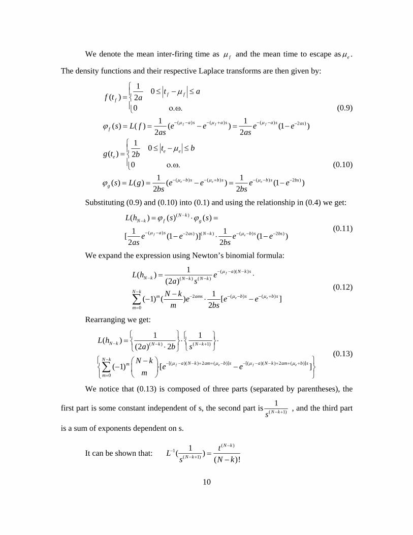
3.1 First Case - Uniform Distributions
In this case we assume both the inter-firing times and the escape time have
Uniform distributions.
10
We denote the mean inter-firing time as fμ and the mean time to escape as eμ .
The density functions and their respective Laplace transforms are then given by:
( ) ( ) ( ) 2 )
1 0( ) 2
01 1( ) ( ) ( ) (1 )
2 2f f f
f ff
a s a s a s asf
t af t a
s L f e e e eas as
μ μ μ
μ
ϕ − − − + − − −
⎧ ≤ − ≤⎪= ⎨⎪ ο.ω.⎩
= = − = −
(0.9)
( ) ( ) ( ) 2 )
1 0( ) 2
01 1( ) ( ) ( ) (1 )
2 2e e e
e ee
b s b s b s bsg
t bg t b
s L g e e e ebs bs
μ μ μ
μ
ϕ − − − + − − −
⎧ ≤ − ≤⎪= ⎨⎪ ο.ω.⎩
= = − = −
(0.10)
Substituting (0.9) and (0.10) into (0.1) and using the relationship in (0.4) we get:
( )
( ) ( )2 ) ( ) 2 )
( ) ( ) ( )
1 1[ (1 )] (1 )2 2
f e
N kN k f g
a s b sas N k bs
L h s s
e e e eas bs
μ μ
ϕ ϕ−−
− − − −− − −
= ⋅ =
− ⋅ − (0.11)
We expand the expression using Newton’s binomial formula:
( )( )( ) ( )
( ) ( )2
0
1( )(2 )
1( 1) ( ) [ ]2
f
e e
a N k sN k N k N k
N kb s b sm ams
m
L h ea s
N k e e em bs
μ
μ μ
− − −− − −
−− − − +−
=
= ⋅
−− ⋅ −∑
(0.12)
Rearranging we get:
( ) ( 1)
[( )( ) 2 ( )] [( )( ) 2 ( )]
0
1 1( )(2 ) 2
( 1) [ ]f e f e
N k N k N k
N ka N k am b s a N k am b sm
m
L ha b s
N ke e
mμ μ μ μ
− − − +
−− − − + + − − − − + + +
=
⎧ ⎫ ⎧ ⎫= ⋅ ⋅⎨ ⎬ ⎨ ⎬⋅ ⎩ ⎭⎩ ⎭⎧ ⎫−⎛ ⎞
− ⋅ −⎨ ⎬⎜ ⎟⎝ ⎠⎩ ⎭
∑ (0.13)
We notice that (0.13) is composed of three parts (separated by parentheses), the
first part is some constant independent of s, the second part is ( 1)
1N ks − + , and the third part
is a sum of exponents dependent on s.
It can be shown that: ( )
1( 1)
1( )( )!
N k
N k
tLs N k
−−
− + =−
11
Recalling from relationship (0.8) that exponents in the s domain are translations in
the time domain we get the final result:
( )
( ) ( )
0
1( )(2 ) 2
1( 1) [( ) ( ) ( ) ( )]( )!
N k N k
N km m N k m m N k m
m
h ta b
N kt U t t U t
m N kβ β β β
− −
−− −
− − + +=
=⋅
−⎛ ⎞− ⋅ ⋅ − ⋅ − − − ⋅ −⎜ ⎟ −⎝ ⎠
∑ (0.14)
Where: ( )( ) 2 ( )
( )( ) 2 ( )
mf e
mf e
a N k am b
a N k am b
β μ μ
β μ μ−
+
= − − + + −
= − − + + +
We can very easily carry out the integration and get:
( )
( 1) ( 1)
0
1( )(2 ) 2
1( 1) [( ) ( ) ( ) ( )]( 1)!
N k N k
N km m N k m m N k m
m
H ta b
N kt U t t U t
m N kβ β β β
− −
−− + − +
− − + +=
=⋅
−⎛ ⎞− ⋅ ⋅ − ⋅ − − − ⋅ −⎜ ⎟ − +⎝ ⎠
∑(0.15)
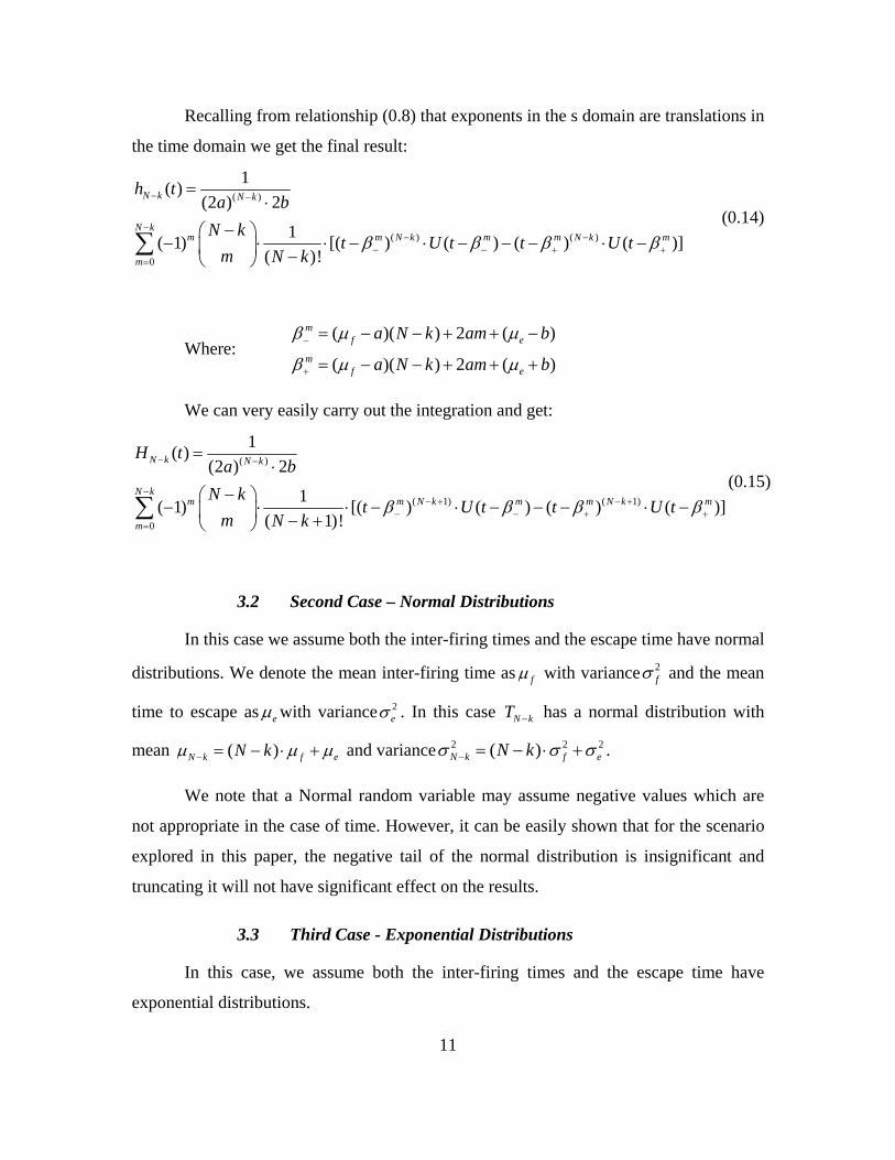
3.2 Second Case – Normal Distributions
In this case we assume both the inter-firing times and the escape time have normal
distributions. We denote the mean inter-firing time as fμ with variance 2fσ and the mean
time to escape as eμ with variance 2eσ . In this case N kT − has a normal distribution with
mean ( )N k f eN kμ μ μ− = − ⋅ + and variance 2 2 2( )N k f eN kσ σ σ− = − ⋅ + .
We note that a Normal random variable may assume negative values which are
not appropriate in the case of time. However, it can be easily shown that for the scenario
explored in this paper, the negative tail of the normal distribution is insignificant and
truncating it will not have significant effect on the results.
3.3 Third Case - Exponential Distributions
In this case, we assume both the inter-firing times and the escape time have
exponential distributions.

12
We denote the mean inter-firing time as 1fλ and the mean time to escape as 1
eλ .
The density functions and their respective Laplace transforms are then given by:
( ) f tf ff t e λλ −= ; ( ) ( ) f
ff
s L fs
λϕ
λ= =
+ (0.16)
( ) ete eg t e λλ −= ; ( ) ( ) e
ge
s L gs
λϕλ
= =+
(0.17)
Substituting (0.16) and (0.17) into (0.1) and using the relationship in (0.4) we get:
( )
( )( )( ) ( ) ( )
( )
N kfN k e
N k f g N kf e
L h s ss s
λ λϕ ϕλ λ
−−
− −= ⋅ = ⋅+ +
(0.18)
We define: ' es sλ= + and substitute into 11)
( ) ( ) ( )
( ) ( ) ( )
( ) ( )
( ) ( )
( )1 1( )( ') ' ( ) ' ( ')
1 ( ')( ') ' ( ' ')
N k N k N kf e f e f e
N k N k N k N kf e f e f e
N k N kf e
N k N k
L hs s s s
s s
λ λ λ λ λ λλ λ λ λ λ λ
λ λ λλ λ
− − −
− − − −
− −
− −
⋅ ⋅ −= ⋅ = ⋅ ⋅ =
− + − − +
⎧ ⎫⋅ ⎧ ⎫⎪ ⎪ ⎧ ⎫⋅ ⋅⎨ ⎬ ⎨ ⎬ ⎨ ⎬+⎩ ⎭⎪ ⎪ ⎩ ⎭⎩ ⎭
(0.19)
We notice that (0.19) is the multiplication of three expressions (separated by
parentheses), the first one being independent of s’, the second one is just the inverse of s’
and the third we recognize to be the Laplace transform of the Erlang density function
with parameters N-k, and ' f eλ λ λ= − .
We recall the relationship in (0.7) and so we get the final result.
( ) 1
( )( )
0
(( ) )( ) [1 ]
( ) !f ee
N k mN ktf e f et
N k N kmf e
th t e e
mλ λλ λ λ λ λ
λ λ
− − −− −−
− −=
⋅ −= −
− ∑ (0.20)
The exponent at the beginning of (0.20) is the result of the substitution we made
in (0.18) and the relationship in (0.7).
4. Analysis
Now that we have an expression for ( )N k N kH t− − we can calculate the probability
for a timely hit and therefore – by factor multiplication – the probability of killing the
attacker.
13
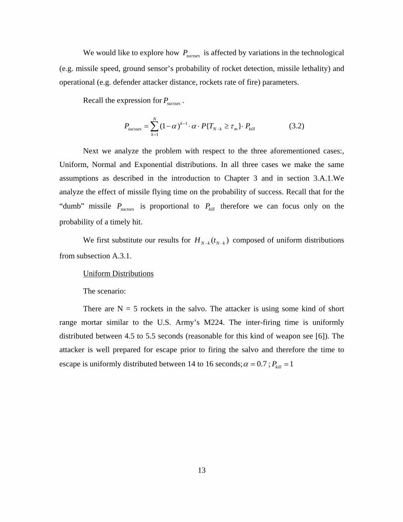
We would like to explore how sucssesP is affected by variations in the technological
(e.g. missile speed, ground sensor’s probability of rocket detection, missile lethality) and
operational (e.g. defender attacker distance, rockets rate of fire) parameters.
Recall the expression for sucssesP .
1
1(1 ) { }
Nk
sucsses N k m killk
P P T Pα α τ−−
=
= − ⋅ ⋅ ≥ ⋅∑ (3.2)
Next we analyze the problem with respect to the three aforementioned cases:,
Uniform, Normal and Exponential distributions. In all three cases we make the same
assumptions as described in the introduction to Chapter 3 and in section 3.A.1.We
analyze the effect of missile flying time on the probability of success. Recall that for the
“dumb” missile sucssesP is proportional to killP therefore we can focus only on the
probability of a timely hit.
We first substitute our results for ( )N k N kH t− − composed of uniform distributions
from subsection A.3.1.
Uniform Distributions
The scenario:
There are N = 5 rockets in the salvo. The attacker is using some kind of short
range mortar similar to the U.S. Army’s M224. The inter-firing time is uniformly
distributed between 4.5 to 5.5 seconds (reasonable for this kind of weapon see [6]). The
attacker is well prepared for escape prior to firing the salvo and therefore the time to
escape is uniformly distributed between 14 to 16 seconds; 0.7α = ; 1killP =
14
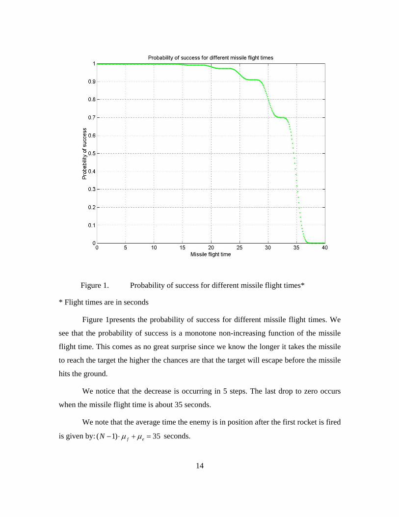
Figure 1. Probability of success for different missile flight times*
* Flight times are in seconds
Figure 1presents the probability of success for different missile flight times. We
see that the probability of success is a monotone non-increasing function of the missile
flight time. This comes as no great surprise since we know the longer it takes the missile
to reach the target the higher the chances are that the target will escape before the missile
hits the ground.
We notice that the decrease is occurring in 5 steps. The last drop to zero occurs
when the missile flight time is about 35 seconds.
We note that the average time the enemy is in position after the first rocket is fired
is given by: ( 1) 35f eN μ μ− ⋅ + = seconds.
15
To understand the behavior of the probability of success as shown in the curve of
Figure 1, let’s explore the probability for a timely hit when there are N-k residual rockets,
given by { } 1 ( )N k m N k mP T Hτ τ− −≥ = − .
The following Figure presents { }N k mP T τ− ≥ for different numbers of residual
rockets N-k, and missile flight time mτ . The scenario parameters are as in Figure 1
Figure 2. Probability of a timely hit for different missile flight times (in seconds) and number of residual rockets*
* To properly read this figure, print in color.
We notice that the probability of a timely hit given the number of rockets left in
the salvo is a sharp step function, in particular for a small number of residual rockets. The
drop moves in the positive direction of the mτ axis for increasing number of residual
rockets.
0 Rockets left
4 Rockets left
16
This makes sense because each rocket left in the salvo increases the average time
till the target escapes and allows more time for the missile to reach its target. We see that
each one of the curves is indeed shifted by about 5 seconds which corresponds to the
mean inter-firing time of the rockets.
We go back now to analyze the behavior of the probability of success in Figure
1Recall from Equation (0.2) that the probability of success is expressed by a sum of
arguments, each one containing the probability for a timely hit given a different number
of residual rockets. Consider now the region in Figure 1 for values greater than 35
seconds. Looking in the corresponding region in Figure 2 we see that the probability for a
timely hit is zero for any possible number of residual rockets (0 to N-1) in this scenario.
When the missile flight time is very long, even detection of the very first rocket (leaving
4 more rockets in the salvo) does not leave enough time for the missile to reach the target
in time.
Now consider the region where mτ is between about 30 and 35 seconds.
According to our scenario the average time between the first rocket launch in the salvo
and the moment the attacker escapes is 35 seconds. On average there are 30 seconds
between the second rocket launch in the salvo and the moment the attacker escapes, and
so on. Notice in Figure 2 that for this [30,35] region of mτ the probability for a timely hit
is non zero if there are 4 rockets left in the salvo, and zero or close to zero if there are less
than 4 rockets left in the salvo, meaning that the first rocket must be detected in order to
have a significant probability of timely hit. In Figure 1, we see a step up in the probability
of success when 35mτ < seconds. If we decrease the missile flight time further we enter a
region in Figure 2 where the probability of timely hit is significantly greater than zero if
the number of rockets left in the salvo is at least 3. This means that in the expression for
the probability of success (0.2) two of the arguments in the sum are now non-zero. This is
why we see another step up in the probability of success as we decrease .mτ
As discussed above, the probability of success decreases in steps when increasing
the missile flight time. However, we notice that the size of each step is not the same; the
last decrement (when mτ increases above 35 sec) being the largest.
17
To understand why this happens we go back to the expression of the probability
of success in Eq.(0.2). We notice that the arguments of the sum are multiplied by a
discrete function of k, 1( ) (1 )kkilld k Pα α−= − ⋅ ⋅ . Since α is between 0 and 1 ( )d k is
monotone increasing with the number of residual rockets. ( )d k controls the step size of
the curve in Figure 1(probability of success), we can now see why the returns for
decreasing the missile flight time are diminishing.
The initial increase in the probability of success (when the missile flight time is
just small enough to give some chance of success), is given by ( )d k for the case when
k=1, which gives: (1) killd Pα= ⋅ . So, if reducing the missile flight time is difficult, and we
want to maximize the initial jump in the probability of success, we should increase α as
much as possible.
At the heart of this qualitative behavior of step decreases in the probability of
success seen in Figure 1, is the fact that we chose time parameters (inter-firing and
escape) with relatively small variances. These small variances lead to uniform cdf close
to a step function. The uniform cumulative distribution becomes close to a step function
whenever we reduce the range between its two parameters relative to their midpoint
(mean). This occurs because the pdf will become close to an impulse function and thus
the cdf will become close to a step function. This in turn makes the
distribution ( )N k N kH t− − resemble a step function.
When we increase the range of the distribution, we increase the variance relative
to the mean of the underlying distributions and we get less steep CDFs. This will change
the discrete jump nature of the curve we see in Figure 1 and make the probability of
success plot ”smoother”.
Figure 3presents the probability of a timely hit for the uniform distribution case
with greater variability. Figure 4presents the resulting probability of successes.
The scenario is:
There are N = 5 rockets in the salvo as before. The attacker uses the same weapon
however he fires at a less regular rate and the inter-firing time is uniformly distributed
18
between 4 to 6 seconds. The time to escape is uniformly distributed between 10 to 20
seconds. Notice that the means of the underlying distributions are still 5 and 15 seconds,
respectively, as before. 0.7; 1killPα = =
Figure 3. Probability of a timely hit for different missile flight times (in seconds) and number of residual rockets (increased variability) *
* To properly read this figure, print in color.
0 Rockets left
4 Rockets left
19
Figure 4. Probability of success for different missile flight times (in seconds) (increased variability)
Exploring the case of normal distributions gives similar results to the uniform
case. Therefore we move directly to the exponential case. Results for the normal case are
presented in appendix A.
Exponential Distributions
An interesting case is the case where both the escape time and the inter-firing
times are exponential random variables. In this case, the mean and the variance are
coupled and the ratio between the mean and the standard deviation is always 1. Therefore
we never achieve the qualitative behavior of step decreases and always get a smooth
curve as in the high variability case above. There is still some effect of diminishing
returns, however; it seems the “knee” of the curve is only achieved for a relatively low
missile flight time. Another interesting observation is that for the exponential case the
20
probability of successes is quite high even for very high values of missile flight time.
This is again due to the high variability imposed by the exponential distribution because
the variance is the square of the mean.
Figure 5and 0present the exponential case. The mean times are the same as in
Figure 3and Figure 4
Figure 5. Probability of a timely hit or different missile flight times (in seconds) and number of residual rockets (Exponential case) *
* To properly read this figure, print in color.
0 Rockets left
4 Rockets left
21
Figure 6. Probability of success for different missile flight times (in seconds) (Exponential case)
5. Tradeoff: Wait or Launch?
Recall that the probability of success depends on two factors: timely hit and
accuracy. So far we assumed perfect accuracy and only looked at the defender’s attempt
to respond as quickly as possible and so increase the probability of timely hit. However,
in reality accuracy is not perfect and by waiting and sampling more rockets in the salvo
the defender may improve his accuracy at the cost of reducing the probability of timely
hit. So the question is wait and improve accuracy while reducing the probability of timely
hit, or launch with lower accuracy but higher probability of timely hit.
Let us now assume that the defender launches the missile after M detections. The
missile will be aimed at the average of the M location estimates. The serial number k of
the rocket after which the missile is launched has a negative binomial distribution with
22
parameters M and α. We further assume that the defender’s missile has a cookie cutter
damage function with lethal radius R:
( )0p r R
d r ≤⎧
= ⎨ ο.ω.⎩ (0.21)
and that the defender’s errors of the estimates of attacker’s location after each rocket
detection are iid circular normal random variables with mean 0μ = and variance 2σ . The
average error of M estimates will then have a mean 0Mμ = and a variance
22M M
σσ =. We
then get the expression for the probability of kill (see also [7]):
2 2
2 22 22( ) e 1 e )
2
Mr MR
killMP d r r dr d pσ σφπσ
− − = ⋅ ⋅ ⋅ = ⋅( −∫∫
(0.22)
We rewrite Eq. (0.2) as follows:
2
22( 1)! (1 ) (1 ( )) (1 )( 1)! ( )!
MRNk M M
success N k mk M
kP H p eM k M
σα α τ−
−−
=
−= ⋅ − ⋅ ⋅ − ⋅ ⋅ −
− ⋅ −∑ (0.23)
0 presents the probability of success for different missile flight times and different
M values. The scenario is the same as in Figure 1; that is, uniform inter-firing and escape
distributions. We choose: 2 1p R σ= = = .
23
Figure 7. Probability of success for different missile flight times (in seconds) and different M values.*
* To properly read this figure, print in color.
We see that if the defender chooses to shoot as early as possible immediately after
the first detection (M = 1) then even a slow flying missile, which takes as long as 35
seconds to reach the attacker, may still hit the attacker with probability of ~0.15. For
1M > this probability is 0. However in this case the maximum probability of success is
about 0.4 for different defender missile flight times. On the other hand, waiting for the
second detection does not allow the defender to use a missile which takes longer than
about 32 seconds to reach the target; however the maximum probability of success is
about 0.62.
M=5 M=4
M=1
M=2
M=3
24
We see that there is a tradeoff between the defender waiting to launch until more
than one rocket has been detected and thus improving the probability of kill vs. the
defender launching the missile as early as possible and saving valuable time. Waiting too
long (M=5) is not beneficial because the loss of valuable time overrides the gain in
accuracy and the net result is a low probability of success. The dashed black line marks
the maximal value over all 5 curves. We see that if the defender has a very fast missile
( 15mτ ≤ sec), the defender should wait for 3 detections before launching the missile.
However if the defender has a missile which takes more than about 15 seconds to reach
the target but less than 25 seconds, he should wait for only 2 detections, and if the
missile takes longer than about 25 seconds the defender should launch his missile
immediately after the first detection.
There is another element influencing the probability of success beside the
probability of timely hit and accuracy. This other element is the probability of missile
launch. Notice that in our formulation for every value of M there is some chance that no
more than M-1 rockets will be detected, in which case the missile is not launched at all.
Consider the region in 0where 0mτ = . Obviously a timely hit is guaranteed in this case.
One might expect the curves to be ordered such that the most “accurate” missile ( 5)M =
will be on top, and the least “accurate” missile ( 1)M = at the bottom. However we see
that the curve with the lowest probability of success is the one where 5M = and the
missile is the most accurate. We get this result because the event 5 out of 5 rockets
detected is less likely than for instance than the event 1 out of 5 rockets detected. Figure 8
presents the case where the probability of rocket detection is 1. The rest of the scenario is
just as in 0 Notice when 0mτ = the curves are ordered by M from top to bottom. We
notice that in this case the defender’s best policy changes, and for low values of mτ the
defender should wait for 4 or even 5 detected rockets before launching his missile.
25
Figure 8. Probability of success for different missile flight times (in seconds) and different M values.* (Perfect detection)
* To properly read this figure, print in color.
0 presents the probability of success for different missile flight times and different
M values for the exponential case, that is exponential inter-firing and escape distributions.
The mean inter-firing time and escape time are 5 and 15 seconds respectively. We
choose: 2 1p R σ= = =
M=5
M=1
M=2
M=3
M=4
26
Figure 9. Probability of success for different missile flight times (in seconds) and
different M values.* (Exponential case)
* To properly read this figure, print in color.
Just as in Figure 6, we note that the curves in the exponential case are smoother
and with a longer “tail” than in the uniform case. This is due to the greater variability in
the exponential case and to the pdf’s shape. Comparing 0 with 0 , we find great similarity
between the two figures. We find the same curves intersect with each other in both
figures (for instance 1M = intersect 2,3& 4M = in both figures), a lower M allows the
defender to use a slower missile and so on. In both cases we see that given a very fast
missile the best policy of the defender is to launch after 3M = detected rockets; for a
slower missile the defender should launch after 2M = detected rockets; and for a very
slow missile the defender should launch at 1M = . However, in the exponential case the
region of mτ where 2M = is the best policy extends from ~ 5mτ to ~ 40mτ . Even
beyond ~ 40mτ where 1M = is the best option for the defender, the difference in the
M=5
M=4
M=1
M=2
M=3
27
probability of success between 1M = and 2M = seems insignificant. It would seem then
that in the exponential case, if there is some ambiguity regarding mτ the defender’s “best
bet” would be to launch after 2M = detected rockets.
B. GROUND SENSOR AND “SMART” MISSILE
1. Assumptions
So far, we have assumed that once the missile has been launched it cannot get any
more information about the location of the target. In our model this assumption was
implicit in the fact that killP was fixed regardless of the number of residual rockets or the
value of mτ .
We now assume that the defender has a “smart” missile, meaning that the missile
has an in-flight guiding mechanism. The “smart” missile may use new information
gathered while it is airborne. This new information may be gathered either by the ground
sensor or by an onboard sensor. With this capability, some of the residual rockets in the
salvo may be detected and be used to improve the estimation of the target location. The
improved estimate may enhance the accuracy of the missile and result in higher value
of killP .
Recall that for the “dumb” missile killP is fixed regardless of the number of
rockets that are launched during the missile’s flight. The question now is what will be the
behavior of killP for the “smart” missile.
First, we notice that killP for the “smart” missile is not smaller than killP for the
“dumb” missile. This is true because the “dumb” missile may be considered as a special
case of the “smart” missile. In this special case no new information is gathered (i.e. the
sensor providing the new in-flight information is very poor).
Second, we note that killP must be monotone non-decreasing in the number of
residual rockets. The larger the number of residual rockets, the more opportunities there
are to obtain additional observations for estimating the target location and thus improve
28
the trajectory of the defender’s missile and enhance its accuracy and effectiveness. We
therefore conclude that ( )killP N k− is a monotone non-decreasing function of N-k, the
number of residual rockets.
Finally, we note that killP must also be a monotone non-decreasing function of mτ .
Information gathered after the missile has reached its target is lost and cannot change the
missile’s trajectory. Therefore only rockets launched during the missile’s flight can help
improve its effectiveness. The longer mτ the more opportunities there are for detecting
residual rockets.
To capture the full picture we should consider the probability of kill to be a
function of both the number of residual rockets and of the missile flight time. However
finding an analytically tractable closed form expression for ( , )kill mP N k τ− is difficult (in
most cases); we therefore adopt a different approach, using a simulation, to explore our
model. The simulation is described in detail in Chapter IV.
2. Ground Sensor Guided “Smart” Missile (Method 1)
We first explore the case where the “smart” missile receives new information
gathered by the ground sensor. Following the same arguments as in section 3.A.5 we find
an expression for the probability of kill similar to the one in Eq. (0.22). However, now we
consider not only the number of rockets detected prior to the defender’s missile launch
but also the number L of rockets detected out of V rockets fired while the missile was
airborne. We obtain the following expression:
2
2( )
21 e )M L R
killP p σ+
− = ⋅( − (0.24)
We revise (0.23) and obtain the following expression:
2
2( )
2
0 0
1(1 ) (1 ( )) { | , } (1 ) (1 )
1
M L RN N k Vk M M v L L
success N k m mk M v L
k vP H P V v N k p e
M Lσα α τ τ α α
+− −− −
−= = =
−⎛ ⎞ ⎛ ⎞= ⋅ − ⋅ ⋅ − ⋅ = − ⋅ − ⋅ ⋅ ⋅ −⎜ ⎟ ⎜ ⎟−⎝ ⎠ ⎝ ⎠∑ ∑ ∑ (0.25)
Finding a general expression for { | , }mP V v N k τ= − when the underlying
distribution are Uniform, is quite difficult and so we will use the simulation as mentioned
above.
29
Let us look first at the case of the smart missile launched after 1M = detected
rocket. Figure 10presents the estimated probability of success for a ground sensor guided
“smart” missile, launched after 1M = detected rocket. Each estimate is from a single
simulation run containing a sequence of 1000 rocket salvos. The results for the “dumb”
missile we have presented in section 3.A.5 are also presented here. The scenario is the
same as in Figure 1 (Uniform interfering and escape distributions). We assume 2 1.p R σ= = =
30
Figure 10. Simulation estimates* for the Probability of success for a ground sensor guided “smart” missile ( 1)M = and, calculated Probability of success for the
“dumb” missile launched at different number of detections (M) **
* Each estimate is from a single simulation run containing a sequence of 1000
rocket salvos.
**To properly read this figure, print in color.
We see that the probability of success is no longer a monotone decreasing
function in the missile flight time. Instead, it has a mode, starting at a relatively low level,
increasing to a maximal probability of about 0.8 and then dropping to zero.
We recall that in this scenario, the missile has to be in flight to receive any new
information after it has been launched, this accounts for the initial increase in the
probability of success we see in the figure above. As mτ increases there is a higher
chance that additional rockets will be fired during the missile’s flight; additional
M=5
M=1
Smart
31
observations increase killP and finally the probability of success. As the missile flight time
increases, eventually the probability of a timely hit decreases; this in turn decreases the
probability of success and eventually reduces it to zero.
Notice that the “smart” missile with 1M = is always superior to the “dumb”
missile with 1M = . This is because it will always have at least as much information as
the “dumb” missile when launched immediately after the first detection. The probability
of success for the “smart” missile when 1M = drops to zero alongside the probability of
success for the “dumb” missile when 1M = . When 1M = the “smart” missile is
launched as early as possible; its chances for a timely hit are just as good as those of the
“dumb” missile fired immediately after the first detection. For values of mτ lower than
about 5, the probability of success using the “smart” missile with 1M = is the same as
that for the “dumb” missile with 1M = . This makes sense because when mτ is very small,
there is very little chance for another rocket to be detected during the “smart” missile’s
flight. The “smart” missile will then be aimed only based on the single rocket detected by
the ground sensor prior to the missile launch, the same as in the “dumb” missile case with
1M = .
Recall that the maximum of the probability of success for the “dumb” missile
over all values of M ( max( )successMP ), provides us with the best course of action the
defender can take using the “dumb” missile. Comparing successP for the “smart” missile
with 1M = to max( )successMP for the “dumb” missile, we see that for high values of mτ the
“smart” missile with 1M = is more effective than the “dumb” missile, regardless the
value of M. However below a certain value (about 10 sec) of mτ it becomes better to use a
“dumb” missile launched after 3M = detected rockets, than using the “smart” missile
with 1M = . In this case the missile is effectively so fast that there is no need to rush and
launch it early. It is almost guaranteed that a very fast missile will reach its target in time.
However it is less likely that during its short flight more rockets will be launched and
detected.

32
Notice that the peak of the probability of success for the “smart” missile is higher
than max( )successMP for the “dumb” missile. This is because when the defender uses the
“dumb” missile, his best course of action utilizes the information from at most 3 rockets
(he may choose to use the information of more rockets, but the advantage of more
information is lost to the disadvantage of launching too late); however the “smart”
missile is launched as early as possible, and if it is in the air long enough it may use the
information of possibly up to N rockets.
We see that firing the “smart” missile after 1M = detected rocket is not always
better than the “dumb” missile. It is interesting to see what happens if the defender uses
the “smart” ground sensor guided missile and waits to launch it after more than
1M = detected rockets. Each estimate is from a single simulation run containing a
sequence of 1000 rocket salvos. The following figure presents the simulation results for
the probability of success for a ground sensor guided “smart” missile, for different values
of M. Also presented is the curve of the best course of action the defender can take using
the “dumb” missile we have seen in Figure 7 The scenario is the same as in Figure 1
(Uniform inter-firing and escape distributions). We assume 2 1.p R σ= = =
33
Figure 11. Simulation estimates* for the Probability of success for a ground sensor
guided “smart” missile launched at different number of detections (M) **
* Each estimate is from a single simulation run containing a sequence of 1000
rocket salvos.
**To properly read this figure, print in color.
Comparing Figure 7and Figure 11We see that for any given value of M the
“smart” missile is superior to the “dumb” missile. However as M gets higher the
difference between using the “smart” vs. the “dumb” missile diminishes. This is because
the “smart” missile improves on the “dumb” missile by taking advantage of the
opportunities to detect residual rockets while it’s airborne. As M increases there are fewer
such opportunities. In fact there is no difference between the “smart” and the “dumb”
missile when 5M = since there are no residual rockets for the “smart” missile to draw
on. The dash-dot black line marks the maximal value over all 5 curves (for the “smart”
missile). This line provides us with the defender best policy using the smart missile. We
34
see just as with the dumb missile the faster the missile the longer the defender is willing
to wait (higher M). The defender should never wait for more than 3M = detected rockets.
There is no advantage in using the smart missile when mτ is very small because there is
little chance of detecting an additional rocket launch while the missile is airborne.
We notice that in the Uniform distributions case, just as in section 3.A.5 that the
increase and decrease in the probability of success occur in steps due to the low
variability of the distributions we chose.
When the underlying distributions are exponential, it is easier to find an explicit
expression for equation (0.25). When the inter-firing times are Exponential iid random
variables and given k we can say that, min( , )V N k X= − where ~ ( )f mX Poisson λ τ .
Furthermore min( , )L N k Y= − where ~ ( )f mY Poisson α λ τ⋅ is a Poisson distribution.
We can now rewrite (0.25) and get:
2
2( )
2
0
1(1 ) (1 ( )) { | , } (1 )
1
M l RN N kk M M
success N k m mk M l
kP H P L l N k e
Mσα α τ τ+− −
−−
= =
−⎛ ⎞= ⋅ − ⋅ ⋅ − ⋅ = − ⋅ −⎜ ⎟−⎝ ⎠
∑ ∑ (0.26)
Where:
( )
1
0
( )0
!{ | , }1 { | , }
f m lf m
m N k
mi
el N k
lP L l N kP L i N k l N k
λ α τ λ α τ
ττ
− ⋅ ⋅
− −
=
⎧ ⋅ ⋅⎪ ≤ < −⎪= − = ⎨⎪ − = − = −⎪⎩
∑
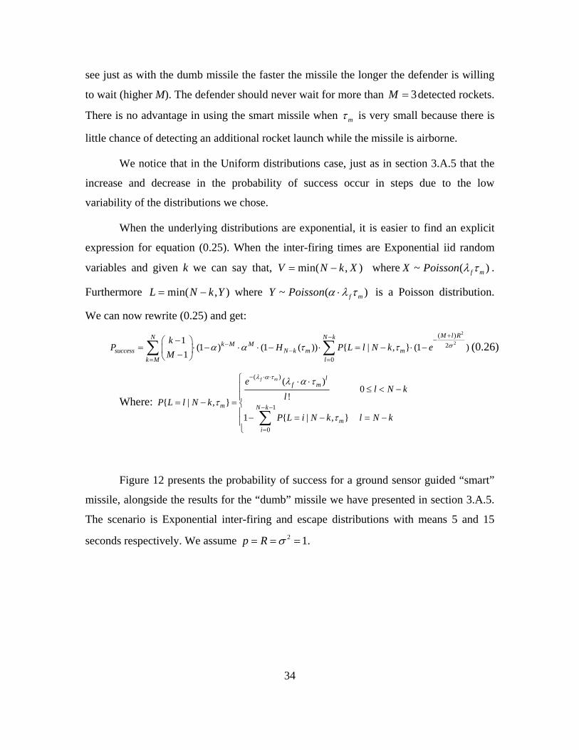
Figure 12 presents the probability of success for a ground sensor guided “smart”
missile, alongside the results for the “dumb” missile we have presented in section 3.A.5.
The scenario is Exponential inter-firing and escape distributions with means 5 and 15
seconds respectively. We assume 2 1.p R σ= = =

35
Figure 12. Probability of success for a ground sensor guided “smart” missile and, for the “dumb” missile launched at different number of detections (M)*
(Exponential case)
* To properly read this figure, print in color.
We find great similarity between Figure 11and Figure 12The ground sensor
guided missile is always superior to the “dumb” missile launched at a given number M of
detected rockets. For higher values of M the “smart” missile loses its advantage over the
“dumb” missile. However, note that the peak probability of success for the “smart”
missile has shifted from to lower values of mτ . For instance for 1M = , the peak
probability of success has moved from ~ 23mτ secs (for the Uniform case) to ~ 15mτ secs
(for the Exponential case). The peak itself is lower for the Exponential case (about 0.62)
then for the Uniform case (about 0.8). Because the inter-firing time in the Exponential
case has greater variability, it may assume higher values than in the uniform case. This
36
reduces the probability of detecting residual rocket fired while the missile is airborne.
The probability of timely hit is lower in the Exponential case than in the Uniform case
(see Figure 2and Figure 5). The net result is a lower peak probability of success than in
the Uniform case.
3. Onboard Sensor “Smart” Missile (Method 2)
We now explore the case where the “smart” missile receives new information
gathered by an onboard sensor.
The onboard sensor presents us with a new situation. We now have to take into
account the improvement in both the probability of rocket detection and the probability of
kill as the sensor moves toward the attacker’s location; the shorter the distance between
the sensor and the launching site, the higher the detection probability and the accuracy of
the target location estimate. We assume that the onboard sensor is able to detect and
measure the attacker’s location at any range and it is not limited by its footprint or
orientation.
It is well known (see [8],[9]) that both parameters – detection probability and
accuracy of location estimate – are related to the signal to noise ratio or the energy
reaching the sensor from its target. We denote this energy as E.
We take the general relationship between the probability of detection and E from
the Albersheim empiric equation (see [8]). We will therefore use the following
relationship:
1
1
exp( )( )1 exp( )d
C EP EC E⋅
=+ ⋅
(0.27)
Where 1C is some normalization-factor, and ( )dP E is the probability of rocket
detection when the sensor receives energy E from the launching site.
Let us assume that the errors of location estimation are iid circular normal random
variables with mean zero and variance 2 ( )Eσ . In [9] it is shown that the variance is
related to E as follows:
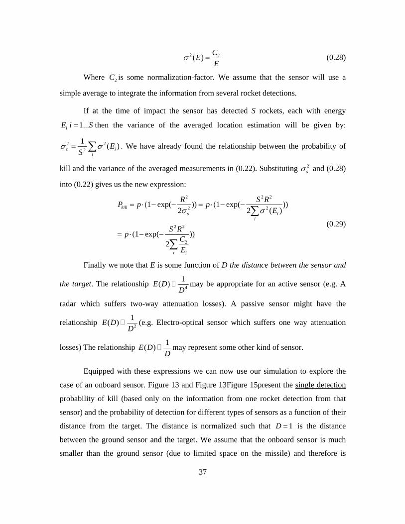
37
2 2( ) CEE
σ = (0.28)
Where 2C is some normalization-factor. We assume that the sensor will use a
simple average to integrate the information from several rocket detections.
If at the time of impact the sensor has detected S rockets, each with energy
1...iE i S = then the variance of the averaged location estimation will be given by:
2 22
1 ( )s ii
ES
σ σ= ∑ . We have already found the relationship between the probability of
kill and the variance of the averaged measurements in (0.22). Substituting 2sσ and (0.28)
into (0.22) gives us the new expression:
2 2 2
2 2
2 2
2
1 exp( )) 1 exp( ))2 2 ( )
1 exp( ))2
kills i
i
i i
R S RP p pE
S Rp CE
σ σ = ⋅ ( − − = ⋅( − −
= ⋅( − −
∑
∑
(0.29)
Finally we note that E is some function of D the distance between the sensor and
the target. The relationship 4
1( )E DD
may be appropriate for an active sensor (e.g. A
radar which suffers two-way attenuation losses). A passive sensor might have the
relationship 2
1( )E DD
(e.g. Electro-optical sensor which suffers one way attenuation
losses) The relationship 1( )E DD
may represent some other kind of sensor.
Equipped with these expressions we can now use our simulation to explore the
case of an onboard sensor. Figure 13 and Figure 13Figure 15present the single detection
probability of kill (based only on the information from one rocket detection from that
sensor) and the probability of detection for different types of sensors as a function of their
distance from the target. The distance is normalized such that 1D = is the distance
between the ground sensor and the target. We assume that the onboard sensor is much
smaller than the ground sensor (due to limited space on the missile) and therefore is
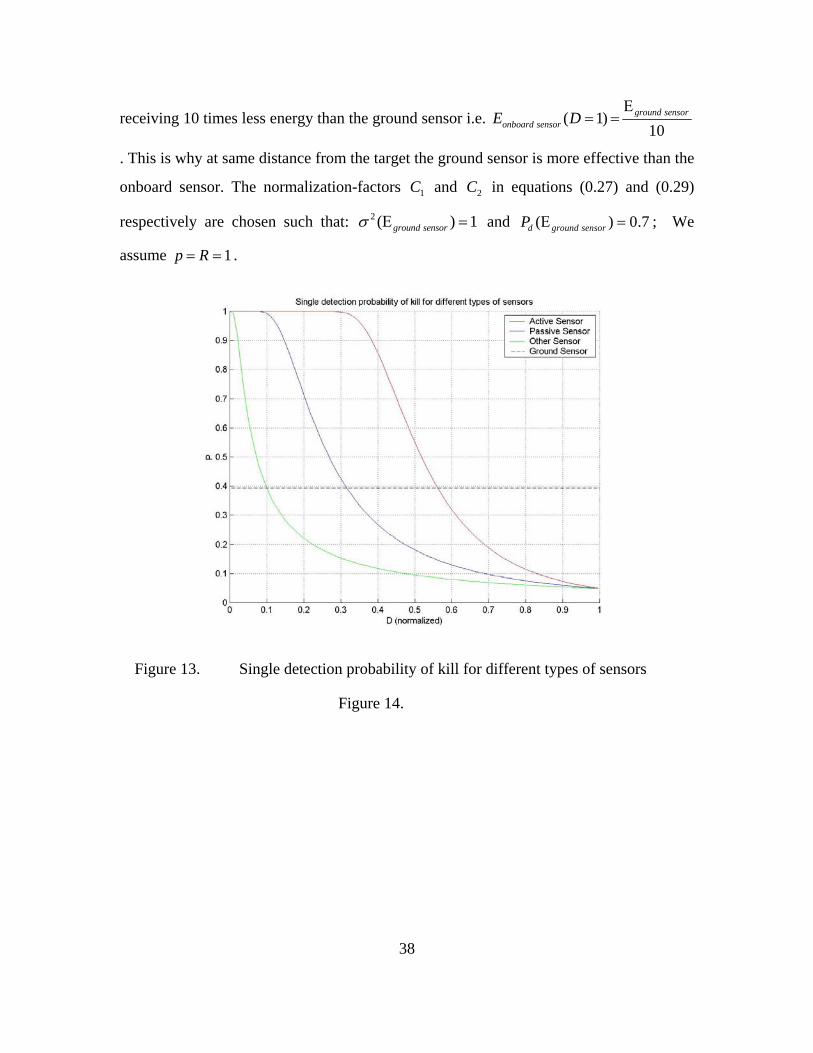
38
receiving 10 times less energy than the ground sensor i.e. ( 1)10
ground sensoronboard sensorE D
Ε= =
. This is why at same distance from the target the ground sensor is more effective than the
onboard sensor. The normalization-factors 1C and 2C in equations (0.27) and (0.29)
respectively are chosen such that: 2 ( ) 1ground sensorσ Ε = and ( ) 0.7d ground sensorP Ε = ; We
assume 1p R = = .
Figure 13. Single detection probability of kill for different types of sensors
Figure 14.
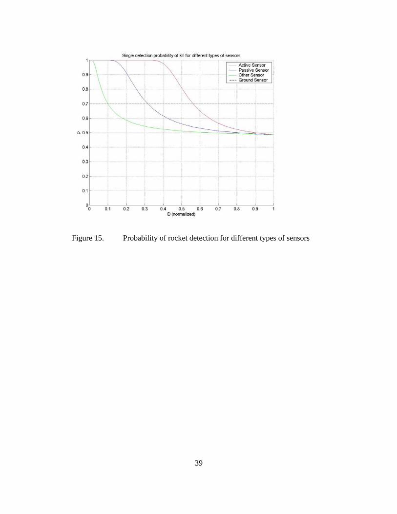
39
Figure 15. Probability of rocket detection for different types of sensors
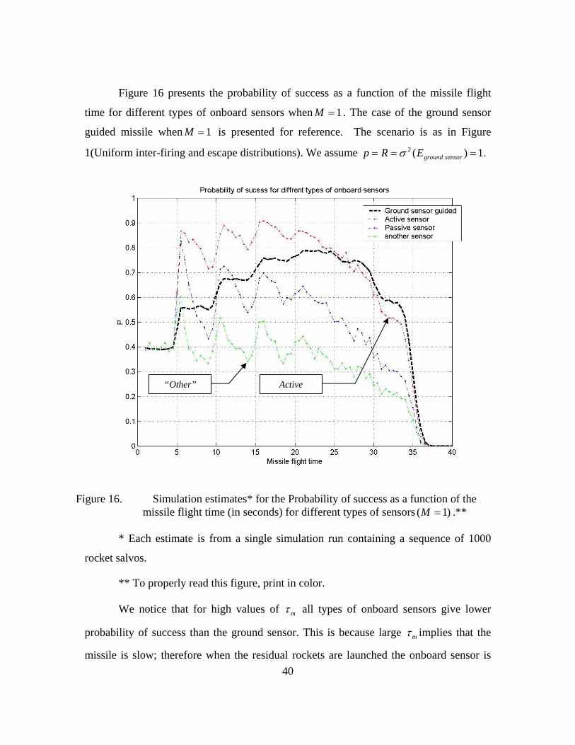
40
Figure 16 presents the probability of success as a function of the missile flight
time for different types of onboard sensors when 1M = . The case of the ground sensor
guided missile when 1M = is presented for reference. The scenario is as in Figure
1(Uniform inter-firing and escape distributions). We assume 2 ( ) 1.ground sensorp R Eσ = = =
Figure 16. Simulation estimates* for the Probability of success as a function of the missile flight time (in seconds) for different types of sensors ( 1)M = .**
* Each estimate is from a single simulation run containing a sequence of 1000
rocket salvos.
** To properly read this figure, print in color.
We notice that for high values of mτ all types of onboard sensors give lower
probability of success than the ground sensor. This is because large mτ implies that the
missile is slow; therefore when the residual rockets are launched the onboard sensor is
“Other” Active
41
more likely to be relatively far away from its destination. Because the sensor is far away
from the target the overall information it provides (as determined by the number of
residual rockets detected and the measurement errors they have) is less than the
information that the ground sensor would have provided. However as mτ becomes
smaller (and the missile is faster), we see that the probability of success for the onboard
sensor increases (although not in a monotone fashion) until it goes above the probability
of success for the ground sensor guided missile. Finally, as in the case of the ground
sensor guided missile, when mτ is small enough the missile is so fast that no rockets are
launched or detected during the missile’s flight; the resulting probability of success has
the same value as if the missile was “dumb”.
We note that the probability of success now has more than one mode. For instance
for all onboard sensors, there is a gradual decrease in the probability of success
when5 10mτ≤ ≤ , then around 10mτ = there is a sharp increase in the probability of
success. As we increase mτ from 5 to 10, the missile becomes slower; the rockets
launched during its flight are detected further away from the missile. For this reason the
rockets become harder for the onboard sensor to detect and when detected they provide
less information and have a less effect on the probability of kill. However since the inter-
firing time is uniform between 4.5 and 5.5 seconds, during a flight time of less than 10
seconds no more than 2 rockets may be launched and detected. As we increase mτ beyond
10 seconds, the opportunity to detect a third rocket arises; the extra rocket will provide
more information which causes a spike in the probability of success. This ripple effect
would not have been so distinct had we chosen inter-firing times with a greater range.
For the scenario described above, we see it is not beneficial to use an on-board
sensor, unless we have a relatively fast missile.
Figure 17 presents the probability of success as a function of the missile flight
time for different types of onboard sensors when 1M = , for the Exponential case. The
42
case of the ground sensor guided missile when 1M = is presented for reference. The
scenario is Exponential inter-firing and escape distributions with means 5 and 15 seconds
respectively. We assume 2 ( ) 1.ground sensorp R Eσ = = =
Figure 17. Simulation estimates* for the Probability of success as a function of the missile flight time (in seconds) for different types of sensors ( 1)M = .**
(Exponential case)
* Each estimate is from a single simulation run containing a sequence of 1000
rocket salvos.
**To properly read this figure, print in color.
Notice that in the exponential case, when the onboard sensor receives 10 times
less energy than the ground sensor, there is hardly any difference between the probability
of success if the missile is guided by the ground sensor or by the “Active” onboard
“Other”
Active
43
sensor. The active sensor does do slightly better than the ground sensor for ~ 10mτ secs.
It seems that in this case investing in the development of an onboard sensor is not
beneficial.
Finally, we explore the defender’s option to wait for M detected rockets before
launching the missile. The next 4 figures present the probability of success for the
onboard sensor “smart” missile after different number M of detected rockets, for “Active”
and “Passive” sensor. The scenario in 0and 0is Uniform distributions as in Figure 1 The
scenario in Figure 20and Figure 21is Exponential inter-firing and escape time with means
5 seconds and 15 seconds respectively.
Figure 18. Simulation estimates* for the Probability of success as a function of the
missile flight time (in seconds) for onboard “Active sensor, for different values of M.** (Uniform case)
* Each estimate is from a single simulation run containing a sequence of 1000 rocket salvos. ** To properly read this figure, print in color
44
Figure 19. Simulation estimates* for Probability of success as a function of the missile
flight time (in seconds) for onboard “Passive sensor, for different values of M.* (Uniform case)
* Each estimate is from a single simulation run containing a sequence of 1000 rocket salvos. **To properly read this figure, print in color
45
Figure 20. Simulation estimates* for the Probability of success as a function of the
missile flight time for onboard “Active sensor, for different values of M.** (Exponential case)
* Each estimate is from a single simulation run containing a sequence of 1000 rocket salvos. **To properly read this figure, print in color

46
Figure 21. Simulation estimates* for the Probability of success as a function of the
missile flight time for onboard “Passive sensor, for different values of M.** (Exponential case)
* Each estimate is from a single simulation run containing a sequence of 1000 rocket salvos. **To properly read this figure, print in color
Just as with the “dumb” and the ground sensor guided missile, the defender
should never wait for more than 3M = detected rockets in this scenario. The black
dotted curve is the “best policy” curve for the onboard sensor. Also plotted for reference
are the “best policy” curves for the “dumb” and the ground sensor guided missiles. Note
that the passive onboard sensor missile is always inferior to the ground sensor guided
missile (under these scenarios). The “Active” onboard sensor missile does a little better
than the ground sensor guided missile in the Uniform case, but in the Exponential case
there is no distinguishable difference between the two.
47
IV. THE CASE OF FALSE POSITIVE DETECTIONS - A SIMULATION MODEL
A. INTRODUCING FALSE DETECTIONS
1. Assumptions
In Chapter III, we assumed that the ground based sensor has no false positive
detections. In this chapter we explore how false positive detections (henceforth called, in
short, false detections) affect our proposed tactics.
Generally speaking, every sensor has some false detections, which may be due to
processes internal to the sensor, or due to external conditions such as weather or
interference caused by other systems. In our model we assume that the times between
two consecutive false detections are iid random variables independent of whether a rocket
has been fired.
We assume that only the ground sensor may have false detections. The missile’s
onboard sensor does not have false detections.
We assume that the ground sensor makes a measurement of the attacker’s location
with circular normal distributed errors and variance 2σ , even when the detection is false.
We make this assumption to simplify the simulation. Obviously, in a real-world situation
false detections may reduce the missile’s accuracy. However this assumption still makes
some sense. In a real situation if the false detection is extremely far away from the
attacker’s location it will not be associated to the salvo. Furthermore, the simulation does
handle the cases when false detections trigger a missile launch while there is no ongoing
salvo at all. As in Chapter III , we assume that the defender launches at most one missile
per salvo.
2. The Firing Rule ˆ ˆ( , )M T
In Chapter III, we assume that the defender fires back a missile as soon as he
detects a rocket within the salvo. In the presence of false detections, such a policy may
lead to unnecessary missile launches whenever a false detection occurs. Such missile
48
launches are disadvantageous for two reasons. First, they cause waste of missiles, which
may be limited or expensive; and second, it may lead to unnecessary collateral damage as
missiles may hit innocent targets.
To mitigate the problem of unnecessary missile launches, we introduce a new
response policy for the defender. We assume that the defender knows that the attacker
fires his rockets in salvos of several rockets at a time. The defender takes advantage of
this fact and estimates when a salvo has begun by looking for a series of detections close
in time. Following such a cluster of detections, the defender makes a salvo declaration
and fires a missile in response. Such a policy may reduce the rate of launching missiles
unnecessarily since now only false detections which occur in close proximity will lead to
a false salvo declaration and unnecessary missile launches.
The firing rule is defined by the pair ˆ ˆ( , )M T as follows:
Looking at a sliding window in time of size T̂ time units, the defender
declares a salvo the moment the sliding window contains at least M̂ detections,
counting from the last detection accounted for by the previous salvo declaration.
Detections from or before the previous salvo declaration are not counted to reduce
the number of salvo declarations during the same salvo.
We define a positive salvo declaration as a salvo declaration which is made
during a real salvo (from the moment the attacker is in position until he has fired the last
rocket).
3. Problem Definition
For M̂ large enough and T̂ small enough the firing rule may reduce the number
of false declarations, however it introduces two new problems. First, the probability of a
positive salvo declaration is decreased and second, valuable time may be lost waiting for
enough detections to meet the firing rule criteria, thus decreasing the probability of timely
detection.
49
We therefore want to find the firing rule pair ˆ ˆ( , )M T which gives the best tradeoff
between low false salvo declaration rate and high probability of success.
B. SIMULATION DESCRIPTION
Initial attempts to describe the problem in the presence of false detections
analytically did not lead to tractable closed form solutions which lend insights easily. We
therefore chose to approach the problem using discrete event simulation.
1. Events Graphs
To write our simulation we have used discrete event simulation (DES)
methodology and the SimKit programming toolkit (see [10]). DES simulations maintain a
list of scheduled events. Each event may affect system variables, schedule future events
or, cancel future events. DES simulations are represented by events graphs. The
following figure presents a simple example of a DES event graph.
Figure 22. Event graph example
In the simple event graph above, there are two types of events represented by
circles: doFoo and doBar(a).
The description of each event is described in a rectangular frame attached to the
event by a broken line. doFoo increments the system variable numberOfFoos and
50
instantiates the variable “a”. doFoo adds “a” (received from its argument) to the system
variable numberOfBars. The arc connecting the two events is a scheduling arc. The arc
will schedule a doBar(a) event some time units after the execution time of doFoo. The
time of scheduling will be determined by the distribution of tbar written next to the arc
with no parentheses. If no time distribution is written next to the arc, the scheduled event
will be scheduled at the same time as the scheduling event. A doBar(a) event will only be
scheduled if the condition numberOfFoos is greater than numberOfBars, is met. The arc
conditioning is written in parentheses next to the scheduling arc. the event doFoo passes
the variable “a” to the event “doBar(a), written in rectangular frame next to the
scheduling arc.
For further reading on SimKit and DES see [10].
2. The Simulation Model
The following two figures present our DES event graph. Because of it size, the
event graph is divide into two figures, the events marked in red are common to both
figures.
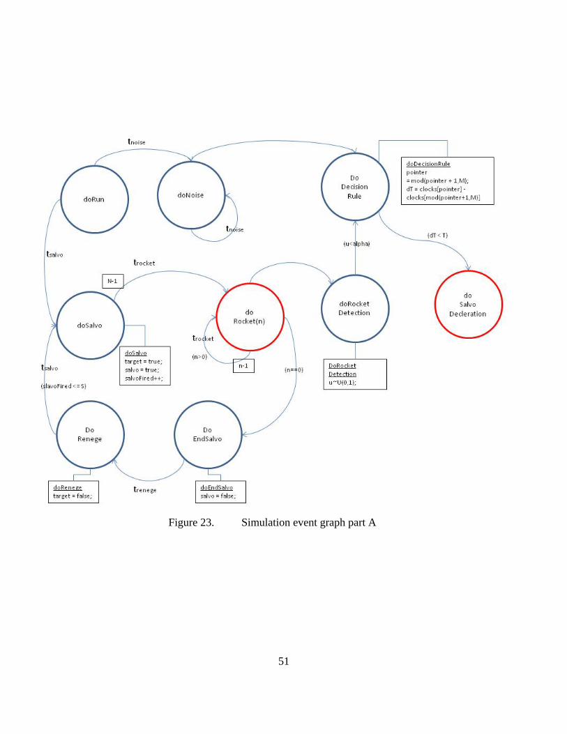
51
Figure 23. Simulation event graph part A
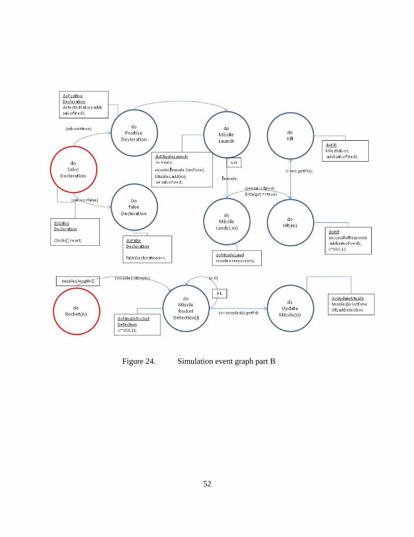
52
Figure 24. Simulation event graph part B
53
C. ANALYSIS
1. Positive Salvo Declaration as a Function of the Firing Rule ˆ ˆ( , )M T
Our MOE is the proportion of positive salvo declarations among the total number
of salvos. This MOE estimates the sensitivity of our firing rule – the conditional
probability of detecting a salvo on time. We call this MOE the probability of positive
salvo declaration.
The scenario parameters are:
The missile is “Dumb”. There are N = 5 rockets in the salvo. The inter-firing time
is uniformly distributed between 4.5 to 5.5 seconds. The time to escape is uniformly
distributed between 14 to 16 seconds; The probability of rocket detection is 0.7α = ; to
find the conditional probability of kill we use a cookie cutter damage function with
parameters 2 1p R= = . We assume the location estimate errors are iid circular normal
r.v. with variance 2 1σ = . The time between salvos, and the time between false detections
are exponentially distributed with mean 7200 seconds (2 hours), and 900 seconds (15
min) respectively. The missile flight time 20mτ = seconds is fixed.
Figure 25presents the probability of positive salvo declaration for different fireing
rules.
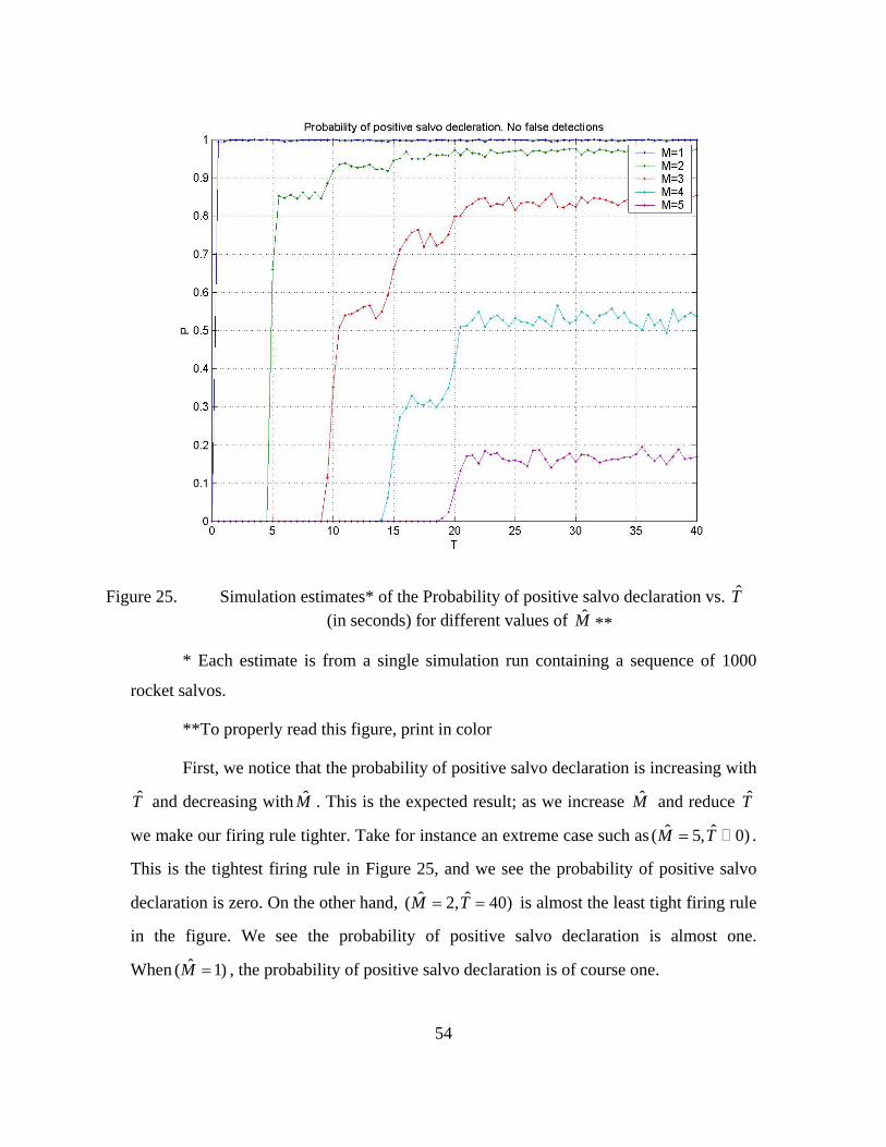
54
Figure 25. Simulation estimates* of the Probability of positive salvo declaration vs. T̂ (in seconds) for different values of M̂ **
* Each estimate is from a single simulation run containing a sequence of 1000
rocket salvos.
**To properly read this figure, print in color
First, we notice that the probability of positive salvo declaration is increasing with
T̂ and decreasing with M̂ . This is the expected result; as we increase M̂ and reduce T̂
we make our firing rule tighter. Take for instance an extreme case such as ˆ ˆ( 5, 0)M T= .
This is the tightest firing rule in Figure 25, and we see the probability of positive salvo
declaration is zero. On the other hand, ˆ ˆ( 2, 40)M T= = is almost the least tight firing rule
in the figure. We see the probability of positive salvo declaration is almost one.
When ˆ( 1)M = , the probability of positive salvo declaration is of course one.
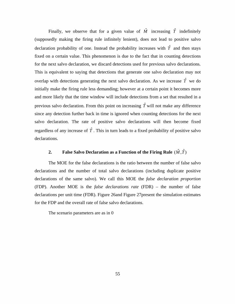
55
Finally, we observe that for a given value of M̂ increasing T̂ indefinitely
(supposedly making the firing rule infinitely lenient), does not lead to positive salvo
declaration probability of one. Instead the probability increases with T̂ and then stays
fixed on a certain value. This phenomenon is due to the fact that in counting detections
for the next salvo declaration, we discard detections used for previous salvo declarations.
This is equivalent to saying that detections that generate one salvo declaration may not
overlap with detections generating the next salvo declaration. As we increase T̂ we do
initially make the firing rule less demanding; however at a certain point it becomes more
and more likely that the time window will include detections from a set that resulted in a
previous salvo declaration. From this point on increasing T̂ will not make any difference
since any detection further back in time is ignored when counting detections for the next
salvo declaration. The rate of positive salvo declarations will then become fixed
regardless of any increase of T̂ . This in turn leads to a fixed probability of positive salvo
declarations.
2. False Salvo Declaration as a Function of the Firing Rule ˆ ˆ( , )M T
The MOE for the false declarations is the ratio between the number of false salvo
declarations and the number of total salvo declarations (including duplicate positive
declarations of the same salvo). We call this MOE the false declaration proportion
(FDP). Another MOE is the false declarations rate (FDR) – the number of false
declarations per unit time (FDR). Figure 26and Figure 27present the simulation estimates
for the FDP and the overall rate of false salvo declarations.
The scenario parameters are as in 0
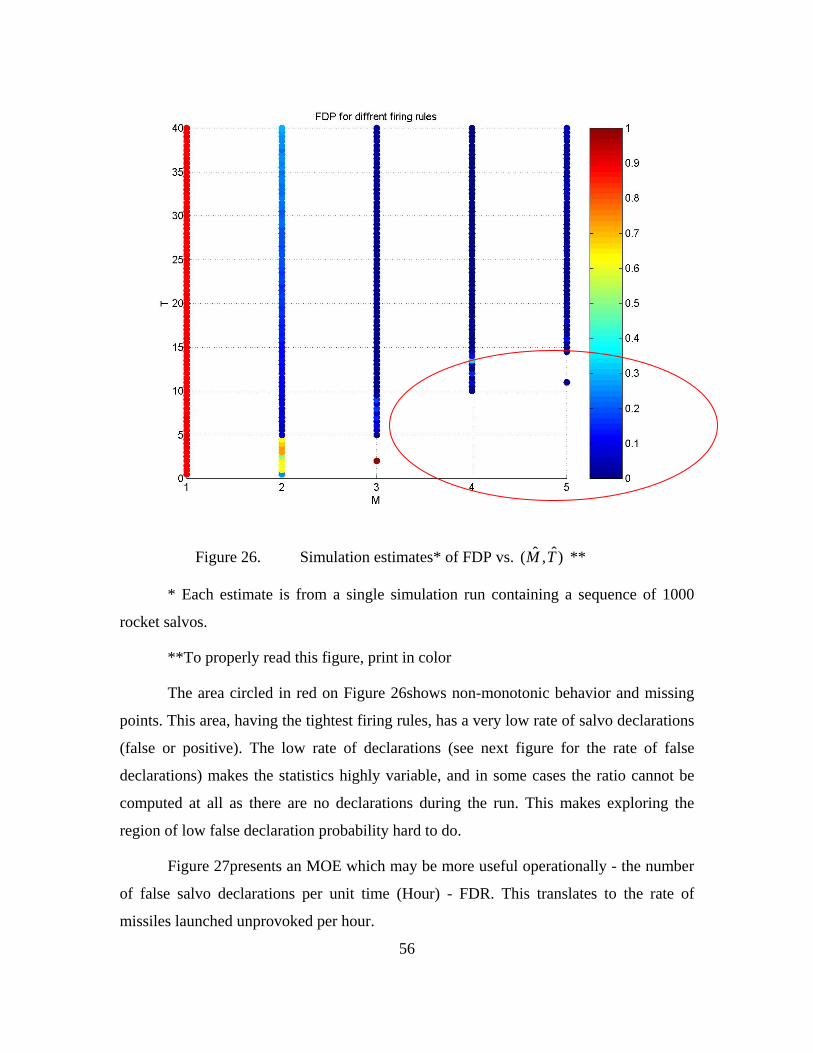
56
Figure 26. Simulation estimates* of FDP vs. ˆ ˆ( , )M T **
* Each estimate is from a single simulation run containing a sequence of 1000
rocket salvos.
**To properly read this figure, print in color
The area circled in red on Figure 26shows non-monotonic behavior and missing
points. This area, having the tightest firing rules, has a very low rate of salvo declarations
(false or positive). The low rate of declarations (see next figure for the rate of false
declarations) makes the statistics highly variable, and in some cases the ratio cannot be
computed at all as there are no declarations during the run. This makes exploring the
region of low false declaration probability hard to do.
Figure 27presents an MOE which may be more useful operationally - the number
of false salvo declarations per unit time (Hour) - FDR. This translates to the rate of
missiles launched unprovoked per hour.
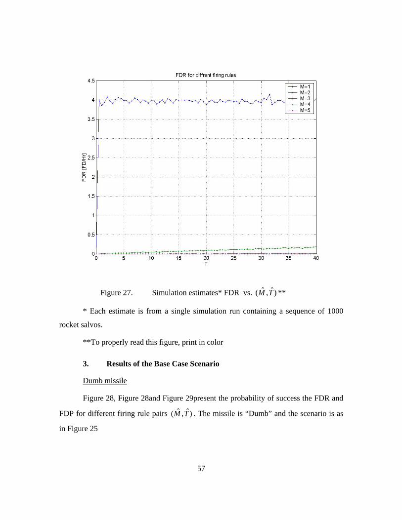
57
Figure 27. Simulation estimates* FDR vs. ˆ ˆ( , )M T **
* Each estimate is from a single simulation run containing a sequence of 1000
rocket salvos.
**To properly read this figure, print in color
3. Results of the Base Case Scenario
Dumb missile
Figure 28, Figure 28and Figure 29present the probability of success the FDR and
FDP for different firing rule pairs ˆ ˆ( , )M T . The missile is “Dumb” and the scenario is as
in Figure 25
58
The probability of success is defined here as in Chapter III. The simulation
estimate for the probability of success is the ratio between the number of salvos the
attacker has been killed and the total number of salvos.
Figure 28. Simulation estimates* for the Probability of success vs. T̂ (in seconds) for different values of M̂ (“Dumb” missile)**
* Each estimate is from a single simulation run containing a sequence of 1000
rocket salvos.
**To properly read this figure, print in color.
59
Figure 29. Simulation estimates* of FDR vs. T̂ (in seconds) for different values of M̂ **
* Each estimate is from a single simulation run containing a sequence of 1000
rocket salvos.
**To properly read this figure, print in color.
60
Figure 30. Simulation estimates* of FDP vs. T̂ (in seconds) for different values of M̂ **
* Each estimate is from a single simulation run containing a sequence of 1000
rocket salvos.
**To properly read this figure, print in color.
For clarity of presentation only the cases ˆ 2M ≥ are presented in Figure 28. We
can see in Figure 27 that for the case ˆ 1M = the value of FDR is simply the rate of false
detections as expected. We have not defined the defender’s acceptable value of FDR, but
it seems obvious that choosing ˆ 1M = (effectively responding to the first detection) is
unacceptable due to the high value of FDR [ / ](4 )FD Hr . The highest probability of success
(~0.55) may be achieved when ˆ 2M = however when ˆ 2M = there is still a significant
FDR. Since the FDR is monotone increasing with T̂ , we may want to choose T̂ slightly
above 5 seconds. This will give the lowest value of FDR possible [ / ](0.02 )FD Hr for a non
61
zero probability of success (~0.45). Alternatively the defender may decide to settle for
lower probability of success and choose ˆ ˆ( 3, 10)M T= > . The FDR is then close to zero
[ / ]( 0.005 )FD Hr< and the probability of success between 0.3 and 0.4.
Method 1: Ground Sensor Guided Missile
The following figure presents the simulation estimates of the probability of
success for the ground sensor guided missile. The rest of the scenario is as in Figure 28
Figure 31. Simulation estimates* of the Probability of success for vs. T̂ (in seconds) for
different values of M̂ (“Smart” ground sensor guided missile)**
* Each estimate is from a single simulation run containing a sequence of 1000
rocket salvos.
**To properly read this figure, print in color.
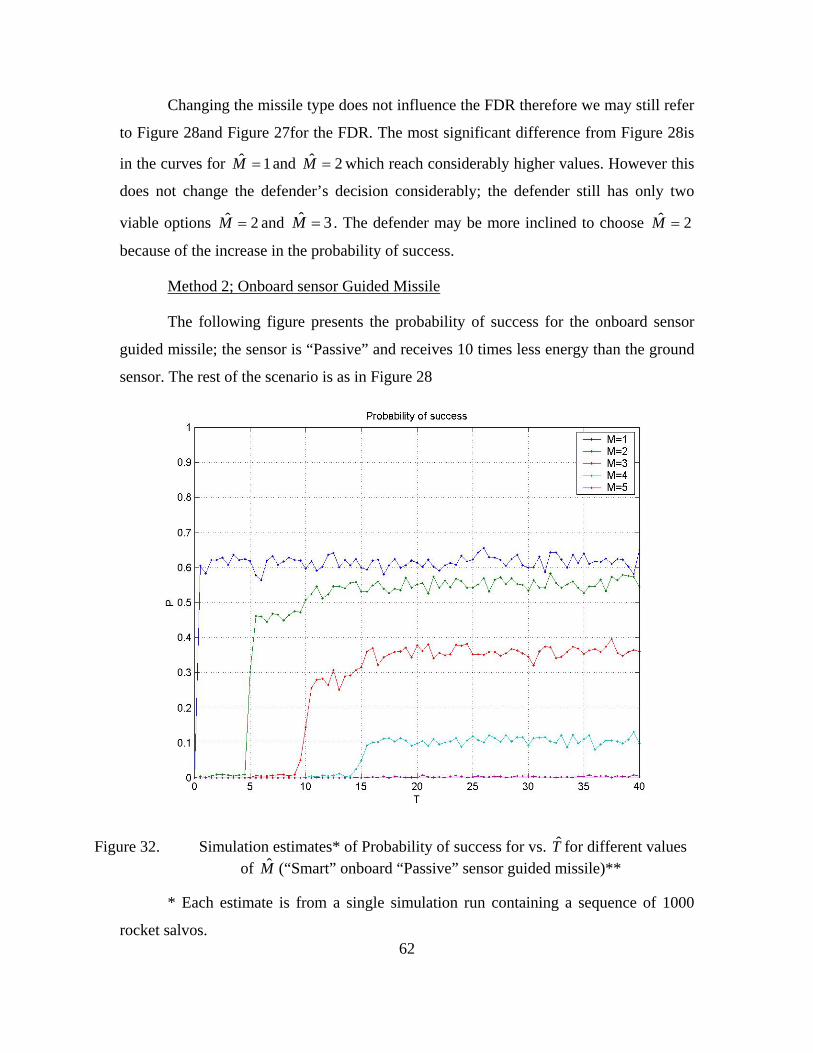
62
Changing the missile type does not influence the FDR therefore we may still refer
to Figure 28and Figure 27for the FDR. The most significant difference from Figure 28is
in the curves for ˆ 1M = and ˆ 2M = which reach considerably higher values. However this
does not change the defender’s decision considerably; the defender still has only two
viable options ˆ 2M = and ˆ 3M = . The defender may be more inclined to choose ˆ 2M =
because of the increase in the probability of success.
Method 2; Onboard sensor Guided Missile
The following figure presents the probability of success for the onboard sensor
guided missile; the sensor is “Passive” and receives 10 times less energy than the ground
sensor. The rest of the scenario is as in Figure 28
Figure 32. Simulation estimates* of Probability of success for vs. T̂ for different values
of M̂ (“Smart” onboard “Passive” sensor guided missile)**
* Each estimate is from a single simulation run containing a sequence of 1000
rocket salvos.
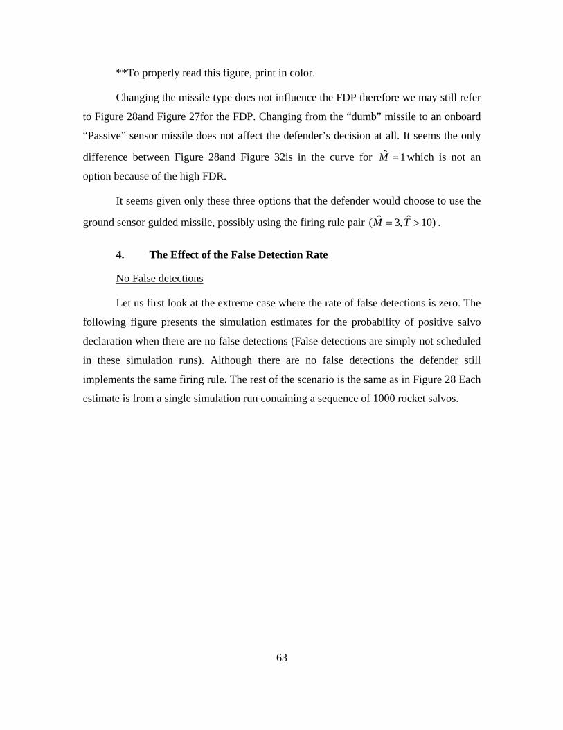
63
**To properly read this figure, print in color.
Changing the missile type does not influence the FDP therefore we may still refer
to Figure 28and Figure 27for the FDP. Changing from the “dumb” missile to an onboard
“Passive” sensor missile does not affect the defender’s decision at all. It seems the only
difference between Figure 28and Figure 32is in the curve for ˆ 1M = which is not an
option because of the high FDR.
It seems given only these three options that the defender would choose to use the
ground sensor guided missile, possibly using the firing rule pair ˆ ˆ( 3, 10)M T= > .
4. The Effect of the False Detection Rate
No False detections
Let us first look at the extreme case where the rate of false detections is zero. The
following figure presents the simulation estimates for the probability of positive salvo
declaration when there are no false detections (False detections are simply not scheduled
in these simulation runs). Although there are no false detections the defender still
implements the same firing rule. The rest of the scenario is the same as in Figure 28 Each
estimate is from a single simulation run containing a sequence of 1000 rocket salvos.
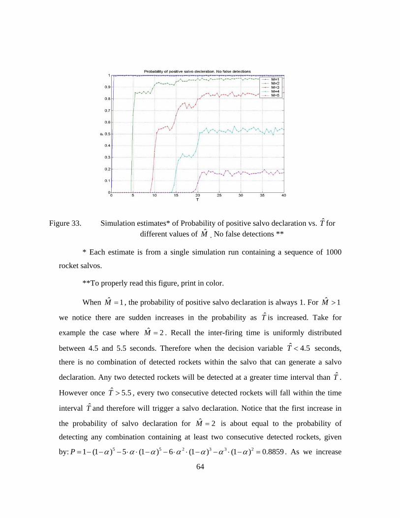
64
Figure 33. Simulation estimates* of Probability of positive salvo declaration vs. T̂ for different values of M̂ . No false detections **
* Each estimate is from a single simulation run containing a sequence of 1000
rocket salvos.
**To properly read this figure, print in color.
When ˆ 1M = , the probability of positive salvo declaration is always 1. For ˆ 1M >
we notice there are sudden increases in the probability as T̂ is increased. Take for
example the case where ˆ 2M = . Recall the inter-firing time is uniformly distributed
between 4.5 and 5.5 seconds. Therefore when the decision variable ˆ 4.5T < seconds,
there is no combination of detected rockets within the salvo that can generate a salvo
declaration. Any two detected rockets will be detected at a greater time interval than T̂ .
However once ˆ 5.5T > , every two consecutive detected rockets will fall within the time
interval T̂ and therefore will trigger a salvo declaration. Notice that the first increase in
the probability of salvo declaration for ˆ 2M = is about equal to the probability of
detecting any combination containing at least two consecutive detected rockets, given
by: 5 5 2 3 3 21 (1 ) 5 (1 ) 6 (1 ) (1 ) 0.8859P α α α α α α α= − − − ⋅ ⋅ − − ⋅ ⋅ − − ⋅ − = . As we increase
65
T̂ more combinations of detected rockets may generate a salvo declaration and so the
probability of salvo declaration increases. The maximal probability of salvo declaration
for ˆ 2M = (given when ˆ 20T > ) is about .997 which corresponds to one minus the
probability of that no rocket is detected in the salvo given by: 51 (1 ) 0.9976P α= − − = ,
the only combination which will not trigger a salvo declaration when ˆ 2M = , ˆ 20T > .
High Rate of False Detections
Let us now explore the effect of increasing the ground sensor’s rate of false
detections. The following figure presents the probability of success and the FDP. The
mean time between false detection is 60 seconds. The rest of the scenario is the same as
in Figure 28
Figure 34. Simulation estimates* for the Probability of success vs. T̂ (in seconds) for different values of M̂ (“Dumb” missile).High rate of false detections **
66
Figure 35. Simulation estimates* of FDP vs. T̂ (in seconds) for different values of M̂ . High rate of false detections **
* Each estimate is from a single simulation run containing a sequence of 1000
rocket salvos.
**To properly read these figures, print in color.
Increasing the rate of false detections increases the FDP (compare to Figure 26).
False detections are the cause for false salvo declaration and so this result is expected.
Comparing Figure 34to Figure 28 we see that the probability of success is increased as
well (this is most obvious when ˆ 5M = ). To understand the contribution of false
detections to the probability of success, think of the case when ˆ 4M = . When ˆ 4M = and
in the absence of false detections, the firing rule demands for 4 rockets to be detected.
The probability of this event is not very high 4 5 4 5( (1 ) 5 0.7 0.3 0.7 0.52)N α α α⋅ ⋅ − + = ⋅ ⋅ + ≅ . Furthermore in the uniform distribution
case, if the decision variable T̂ is low enough there will never be enough time for all 4
rockets to be fired within T̂ . This reduces further the probability of salvo declaration.
Indeed we see that in figure Figure 28when ˆ 4M = and ˆ ˆ( 1) 15fT M μ< − ⋅ = then the
67
probability of success is close to zero. However in the presence of false detections, fewer
than 4 rockets in the salvo need to be detected for a salvo to be declared. Therefore
increasing the rate of false detections increases the probability of salvo declaration and in
turn the probability of success. Notice for ˆ 4M = and ˆ10 15T< < in Figure 34 the
probability of success is significant and not close to zero as in Figure 28 We learn from
this discussion that the probability of success presented in Chapter III with no false
detections, gives a lower bound on the maximal probability of success over T̂ for the
case with false detections.
FDP has sudden drops at some values of T̂ . These drops correspond to sudden
increases in the probability of success. As we have seen earlier increasing T̂ allows more
combinations of detected rockets in the salvo to generate a salvo declaration. This
suddenly increases the rate of positive salvo declaration but only slightly changes the rate
of false salvo declarations. The net result is a sudden drop in the FDP.
The “wild” swings in the FDP for low values of T̂ when ˆ 5M = are due to
simulation variability as explained in 4.C.2.
5. The Effect of the Missile Flight Time
The response of the probability of success to variations in the missile flight time
has been shown in Chapter III in the case with no false detections. We have already
concluded that the results in Chapter III give a lower bound on the maximal probability
of success (over T̂ ) with false detections. For relatively low rate of false detections, we
expect the maximal values of the probability of success to be close to the ones in the case
with no false detections. For instance, in Figure 28the maximal probability of success
when ˆ 2M = is about 0.55. Comparison of this value to the probability of success when
ˆ 2M = and 20mτ = in Figure 7shows they are about the same. We can repeat this exercise
for any value of M̂ and for any type of missile (comparing Figure 11to Figure 31 and,
Figure 19 to Figure 32) We demonstrate this one more time by changing the missile flight
time to 2mτ = and again comparing with Figure 7
68
Figure 36. Simulation estimates* of Probability of success for vs. T̂ for different values of M̂ (“Dumb” missile). 2mτ = **
* Each estimate is from a single simulation run containing a sequence of 1000
rocket salvos.
**To properly read this figure, print in color.
6. The Effect of the Salvos Rate
Let us now explore the effect of increasing the rate of salvos. The following two
figures present estimates of the probability of success and the FDP. Each estimate is from
a single simulation run containing a sequence of 1000 rocket salvos. The mean time
between salvos is 900 seconds (15 minutes), a substantial decrease from 2 hours. The rest
of the scenario is the same as in Figure 28
Figure 37and Figure 28are the same. Increasing the salvo rate does not change the
probability of success. Comparing Figure 37and Figure 29we notice the FDP drops
dramatically. Recall the definition of a false salvo declaration basically says a false salvo
declaration is a salvo declaration which occurs during the time between salvos.
Decreasing the mean time between salvos means that for a given time interval during the
69
simulation run, there would be on average more salvos and less time during which false
salvos may occur. Since the firing rule is unchanged the rate of positive salvo
declarations during the salvo and the rate of false salvo declaration between salvos are
unchanged. Overall the simulation run will have more positive salvo declarations and less
false salvo declarations. The net result is a lower FDP. It is interesting to note that
although the FDR has not changed the FDP has changed. If the defender is more
concerned with the ratio of false to positive salvo declarations rather than the rate of false
salvo declarations per unit time, he may choose a less conservative firing rule under a
more intensive rocket attack. In other words when the attacker shoots more salvos, the
defender may become more “happy trigger”. This last observation means that when the
rate of salvo is higher, the defender may choose a more lenient firing rule. Perhaps in the
case above the defender will choose ˆ ˆ( 2, 6)M T= = .
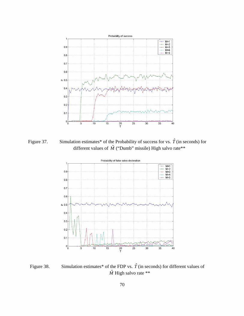
70
Figure 37. Simulation estimates* of the Probability of success for vs. T̂ (in seconds) for different values of M̂ (“Dumb” missile) High salvo rate**
Figure 38. Simulation estimates* of the FDP vs. T̂ (in seconds) for different values of M̂ High salvo rate **
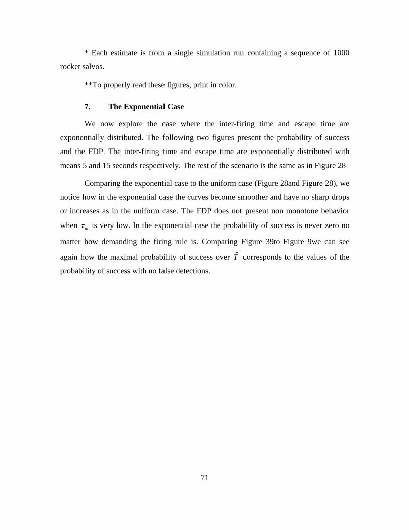
71
* Each estimate is from a single simulation run containing a sequence of 1000
rocket salvos.
**To properly read these figures, print in color.
7. The Exponential Case
We now explore the case where the inter-firing time and escape time are
exponentially distributed. The following two figures present the probability of success
and the FDP. The inter-firing time and escape time are exponentially distributed with
means 5 and 15 seconds respectively. The rest of the scenario is the same as in Figure 28
Comparing the exponential case to the uniform case (Figure 28and Figure 28), we
notice how in the exponential case the curves become smoother and have no sharp drops
or increases as in the uniform case. The FDP does not present non monotone behavior
when mτ is very low. In the exponential case the probability of success is never zero no
matter how demanding the firing rule is. Comparing Figure 39to Figure 9we can see
again how the maximal probability of success over T̂ corresponds to the values of the
probability of success with no false detections.
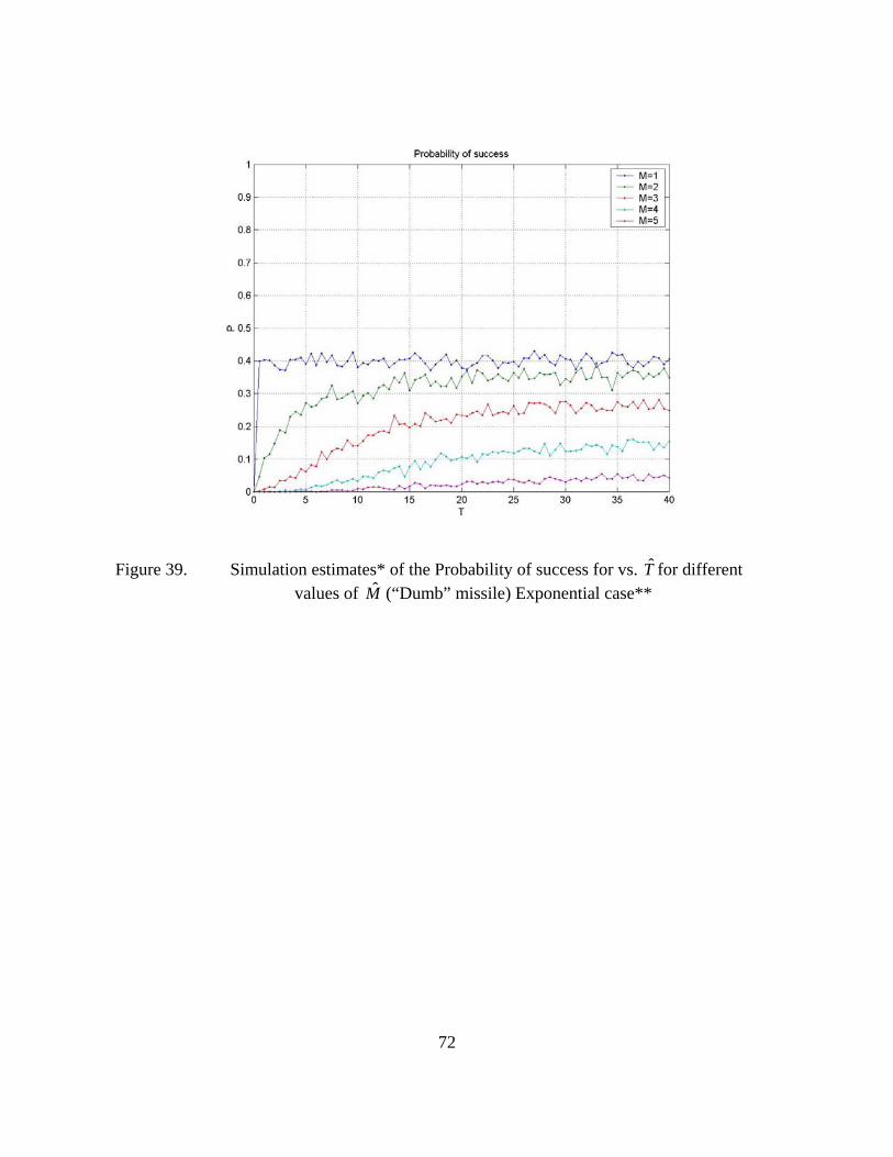
72
Figure 39. Simulation estimates* of the Probability of success for vs. T̂ for different values of M̂ (“Dumb” missile) Exponential case**
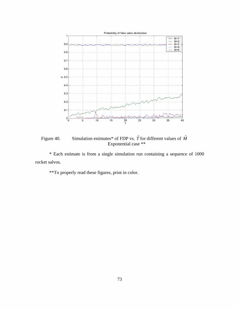
73
Figure 40. Simulation estimates* of FDP vs. T̂ for different values of M̂ Exponential case **
* Each estimate is from a single simulation run containing a sequence of 1000
rocket salvos.
**To properly read these figures, print in color.

74
THIS PAGE INTENTIONALLY LEFT BLANK

75
V. SUMMARY
In this thesis, we have explored and discussed tactical considerations in
countering mortar and rocket fire, when the enemy has adopted a “shoot and scoot”
tactic.
The probability of success – the probability of a timely effective hit of the attacker
– is used as the MOE for the defender’s effectiveness. We have used the probability of
false salvo declaration proportion (FDP) and the false salvo declarations rate (FDR) as
MOEs for the defender’s chances of mistakenly firing a missile and increasing the
collateral damage.
We have developed a tool for comparing different defender tactics and responses
(firing rules). In Chapter III, we have used an analytic model under the assumption that
there are no false detections (and hence zero FDP and FDR). This analytic model allowed
us to quantify the defenders dilemma between waiting, gathering more information and
increasing accuracy, and responding early at the expense of more information and with
less accuracy.
The analytic model presented how the probability of success depends on the
sensor’s probability of rocket detection, the missile flight time and the attacker’s inter-
firing and escape time distributions.
We have explored a suggested new tactic where the defender launches his missile
as soon as possible based on a rough estimate of the attacker’s location. The missile’s
trajectory is later corrected and updated while the missile is airborne, using ground sensor
guidance or different types of onboard sensors. The effectiveness of the suggested tactic
depends on the parameters of the scenario; however it is most useful when the missile
flight time is long compared to the mean salvo length and escape time.
In Chapter IV, we have introduced false detections to the model. To deal with this
predicament we have built a simulation. The defender’s firing rule has been extended to
account for false detections by introducing a sliding time window. The problem in
Chapter IV was to find a firing rule which gives the highest possible probability of

76
success while keeping FDP and FDR as low as possible. It surprising to note that
presence of false detections, actually contributes the defender’s probability of success.
This happens because false detections trigger the defender to launch his missile in cases
he otherwise wouldn’t have, even though a salvo is ongoing (e.g. no rockets were
detected). Of course this improvement comes at the cost of mistakenly firing missiles
causing collateral damage.
We discussed the simulation results for a base case and varied the rate of salvos
the rate of false detections and the missile flight time for sensitivity analysis.
Follow-on research may include taking the salvo rate, inter-firing and escape time
distributions from real life data and exploring the ideas presented in this paper on that
data. It would also be interesting to survey existing weapons and sensors and their
parameters to see if it possible to use any of them for the new tactic suggested in this
thesis.
77
APPENDIX A
Although the results for the Normal case are very similar to the results of the
Uniform case, we present here for the purpose of completeness our results for the case
where the inter-firing and escape time are Normally distributed.
There are N = 5 rockets in the salvo. The inter-firing time is normally distributed
with mean 5 seconds and variance 21 sec12
. The time to escape is normally distributed
with mean 15 seconds and variance 21 sec3
. Notice that the inter firing and escape time
variances and means are the same as in Figure 1The rest of the scenario is as in Figure 1
Figure 41. Probability of success for different missile flight times
78
Figure 42. Probability of a timely hit for different missile flight times and number of residual rockets*
* To properly read this figure, print in color.
As mentioned above comparing Figure 1and Figure 2with Figure 41and Figure
42We see that the results for the Normal case are very similar to the results of the
Uniform case.
0 Rockets left
4 Rockets left
79
LIST OF REFERENCES
[1] I. Ben Israel, “The first missile war Israel-Hizbulla (Summer 2006)” (Hebrew). Tel Aviv University.
[2] A. R. Eckler, S. A. Burr, Mathematical models of target coverage and missile mllocation. MORS 1973.
[3] R. M. Soland, “Optimal terminal defense tactics when several sequential engagements are possible” Operations Research, vol. 35, no. 4 pp. 537-542, July – August 1987.
[4] I. Ravid, “Defense before or after Bomb-Release-Line”, Operations Research, vol. 37, no. 5, pp. 700-715, September - October 1989.
[5] C. W. Sweat “A single-shot noisy duel with detection uncertainty,” Operations Research, vol 19, no. 1, pp. 170-181 January-February, 1971.
[6] “Mortar M224”, U.S. Army fact files, http://www.army.mil/factfiles/equipment/indirect/m224.html
[7] A. R. Eckler, S. A. Burr, Mathematical models of target coverage and missile allocation. MORS 1973, pp. 16-17.
[8] M. L. Skolink, Introduction To Radar Systems. Singapore: McGraw-Hill, 1996, p. 44.
[9] M. L. Skolink, Introduction to radar systems. Singapore: McGraw-Hill, 1996, p. 320.
[10] A. Buss, " Technical Notes Basic Event Graphs Modeling", Simulation News Europe, issue. 31, pp. 1-6, April 2001.

80
THIS PAGE INTENTIONALLY LEFT BLANK
81
INITIAL DISTRIBUTION LIST
1. Defense Technical Information Center Ft. Belvoir, Virginia
2. Dudley Knox Library Naval Postgraduate School Monterey, California
3. Professor Yeo Tat Soon Director, Temasek Defence Systems Institute (TDSI) National University of Singapore Singapore
4. Ms Tan Lai Poh Assistant Manager, Temasek Defence Systems Institute (TDSI) National University of Singapore Singapore
5. Professor Moshe Kress
Operations Research Department Naval Postgraduate School Monterey, California
Related Documents


