NAVAL POSTGRADUATE SCHOOL MONTEREY, CALIFORNIA THESIS Approved for public release; distribution is unlimited DISCOVERY OF BENT FUNCTIONS USING THE FAST WALSH TRANSFORM by Timothy R. O’Dowd December 2010 Thesis Co-Advisors: Jon T. Butler Pantelimon Stanica

Welcome message from author
This document is posted to help you gain knowledge. Please leave a comment to let me know what you think about it! Share it to your friends and learn new things together.
Transcript

NAVAL
POSTGRADUATE SCHOOL
MONTEREY, CALIFORNIA
THESIS
Approved for public release; distribution is unlimited
DISCOVERY OF BENT FUNCTIONS USING THE FAST WALSH TRANSFORM
by
Timothy R. O’Dowd
December 2010
Thesis Co-Advisors: Jon T. Butler Pantelimon Stanica

THIS PAGE INTENTIONALLY LEFT BLANK

i
REPORT DOCUMENTATION PAGE Form Approved OMB No. 0704-0188 Public reporting burden for this collection of information is estimated to average 1 hour per response, including the time for reviewing instruction, searching existing data sources, gathering and maintaining the data needed, and completing and reviewing the collection of information. Send comments regarding this burden estimate or any other aspect of this collection of information, including suggestions for reducing this burden, to Washington headquarters Services, Directorate for Information Operations and Reports, 1215 Jefferson Davis Highway, Suite 1204, Arlington, VA 22202-4302, and to the Office of Management and Budget, Paperwork Reduction Project (0704-0188) Washington DC 20503.
1. AGENCY USE ONLY (Leave blank)
2. REPORT DATE December 2010
3. REPORT TYPE AND DATES COVERED Master’s Thesis
4. TITLE AND SUBTITLE Discovery of Bent Functions Using the Fast Walsh Transform
6. AUTHOR(S) Timothy R. O’Dowd
5. FUNDING NUMBERS
7. PERFORMING ORGANIZATION NAME(S) AND ADDRESS(ES) Naval Postgraduate School Monterey, CA 93943-5000
8. PERFORMING ORGANIZATION REPORT NUMBER
9. SPONSORING /MONITORING AGENCY NAME(S) AND ADDRESS(ES) N/A
10. SPONSORING/MONITORING AGENCY REPORT NUMBER
11. SUPPLEMENTARY NOTES The views expressed in this thesis are those of the author and do not reflect the official policy or position of the Department of Defense or the U.S. Government. IRB Protocol number ______N.A.__________.
12a. DISTRIBUTION / AVAILABILITY STATEMENT Approved for public release; distribution is unlimited
12b. DISTRIBUTION CODE A
13. ABSTRACT (maximum 200 words) Linear cryptanalysis attacks are a threat against cryptosystems. These attacks can be defended against by using combiner functions composed of highly nonlinear Boolean functions. Bent functions, which have the highest possible nonlinearity, are uncommon. As the number of variables in a Boolean function increases, bent functions become extremely rare. A method of computing the nonlinearity of Boolean functions using the Fast Walsh Transform (FWT) is presented.
The SRC-6 reconfigurable computer allows testing of functions at a much faster rate than a PC. With a clock frequency of 100 MHz, throughput of the SRC-6 is 100,000,000 functions per second. An implementation of the FWT used to compute the nonlinearity of Boolean functions with up to five variables is presented.
Since there are 22
n
Boolean functions of n variables, computation of the nonlinearity of every Boolean function with six or more variables takes thousands of years to complete. This makes discovery of bent functions difficult for large n. An algorithm is presented that uses information in the FWT of a function to produce similar functions with increasingly higher nonlinearity. This algorithm demonstrated the ability to enumerate every bent function for n = 4 without the necessity of exhaustively testing all four-variable functions.
15. NUMBER OF PAGES
122
14. SUBJECT TERMS Bent Functions, Cryptography, Field Programmable Gate Array (FPGA), Reconfigurable Computer, Fast Walsh Transform.
16. PRICE CODE
17. SECURITY CLASSIFICATION OF REPORT
Unclassified
18. SECURITY CLASSIFICATION OF THIS PAGE
Unclassified
19. SECURITY CLASSIFICATION OF ABSTRACT
Unclassified
20. LIMITATION OF ABSTRACT
UU
NSN 7540-01-280-5500 Standard Form 298 (Rev. 2-89) Prescribed by ANSI Std. 239-18

ii
THIS PAGE INTENTIONALLY LEFT BLANK

iii
Approved for public release; distribution is unlimited
DISCOVERY OF BENT FUNCTIONS USING THE FAST WALSH TRANSFORM
Timothy R. O’Dowd Lieutenant, United States Navy
B.S., Carnegie Mellon University, 2005
Submitted in partial fulfillment of the requirements for the degree of
MASTER OF SCIENCE IN ELECTRICAL ENGINEERING
from the
NAVAL POSTGRADUATE SCHOOL December 2010
Author: Timothy R. O’Dowd
Approved by: Jon T. Butler Thesis Co-Advisor
Pantelimon Stanica Thesis Co-Advisor
Clark Robertson Chairman, Department of Electrical and Computer Engineering

iv
THIS PAGE INTENTIONALLY LEFT BLANK

v
ABSTRACT
Linear cryptanalysis attacks are a threat against cryptosystems. These attacks can be
defended against by using combiner functions composed of highly nonlinear Boolean
functions. Bent functions, which have the highest possible nonlinearity, are uncommon.
As the number of variables in a Boolean function increases, bent functions become
extremely rare. A method of computing the nonlinearity of Boolean functions using the
Fast Walsh Transform (FWT) is presented.
The SRC-6 reconfigurable computer allows testing of functions at a much faster
rate than a PC. With a clock frequency of 100 MHz, throughput of the SRC-6 is
100,000,000 functions per second. An implementation of the FWT used to compute the
nonlinearity of Boolean functions with up to five variables is presented.
Since there are 22n
Boolean functions of n variables, computation of the
nonlinearity of every Boolean function with six or more variables takes thousands of
years to complete. This makes discovery of bent functions difficult for large n. An
algorithm is presented that uses information in the FWT of a function to produce similar
functions with increasingly higher nonlinearity. This algorithm demonstrated the ability
to enumerate every bent function for n = 4 without the necessity of exhaustively testing
all four-variable functions.

vi
THIS PAGE INTENTIONALLY LEFT BLANK
vii
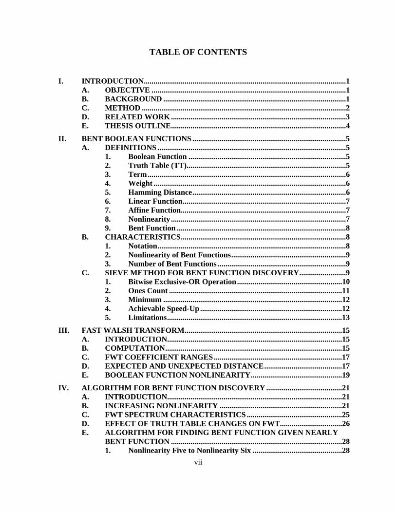
TABLE OF CONTENTS
I. INTRODUCTION........................................................................................................1 A. OBJECTIVE ....................................................................................................1 B. BACKGROUND ..............................................................................................1 C. METHOD .........................................................................................................2 D. RELATED WORK ..........................................................................................3 E. THESIS OUTLINE..........................................................................................4
II. BENT BOOLEAN FUNCTIONS ...............................................................................5 A. DEFINITIONS .................................................................................................5
1. Boolean Function .................................................................................5 2. Truth Table (TT)..................................................................................5 3. Term......................................................................................................6 4. Weight ...................................................................................................6 5. Hamming Distance...............................................................................6 6. Linear Function....................................................................................7 7. Affine Function.....................................................................................7 8. Nonlinearity ..........................................................................................7 9. Bent Function .......................................................................................8
B. CHARACTERISTICS.....................................................................................8 1. Notation.................................................................................................8 2. Nonlinearity of Bent Functions...........................................................9 3. Number of Bent Functions ..................................................................9
C. SIEVE METHOD FOR BENT FUNCTION DISCOVERY........................9 1. Bitwise Exclusive-OR Operation......................................................10 2. Ones Count .........................................................................................11 3. Minimum ............................................................................................12 4. Achievable Speed-Up.........................................................................12 5. Limitations..........................................................................................13
III. FAST WALSH TRANSFORM.................................................................................15 A. INTRODUCTION..........................................................................................15 B. COMPUTATION...........................................................................................15 C. FWT COEFFICIENT RANGES..................................................................17 D. EXPECTED AND UNEXPECTED DISTANCE........................................17 E. BOOLEAN FUNCTION NONLINEARITY...............................................19
IV. ALGORITHM FOR BENT FUNCTION DISCOVERY .......................................21 A. INTRODUCTION..........................................................................................21 B. INCREASING NONLINEARITY ...............................................................21 C. FWT SPECTRUM CHARACTERISTICS .................................................25 D. EFFECT OF TRUTH TABLE CHANGES ON FWT................................26 E. ALGORITHM FOR FINDING BENT FUNCTION GIVEN NEARLY
BENT FUNCTION ........................................................................................28 1. Nonlinearity Five to Nonlinearity Six ..............................................28

viii
2. Nonlinearity Four to Nonlinearity Five ...........................................31
V. COMPUTATION AND ANALYSIS........................................................................33 A. IMPLEMENTATION OF FWT ON SRC-6 ...............................................33
1. About the SRC-6 ................................................................................33 2. Use of the SRC-6 ................................................................................34 3. Limitations of the SRC-6...................................................................35
B. RESULTS AND ANALYSIS OF IMPLEMENTATION OF FWT ON THE SRC-6.....................................................................................................36 1. Nonlinearity for n = 4 ........................................................................36 2. Nonlinearity for n = 5 ........................................................................37 3. Nonlinearity for n = 6 ........................................................................38 4. Trends of Performance Metrics........................................................39
C. IMPLEMENTATION OF ALGORITHM ON PC USING MATLAB ....41
VI. CONCLUSIONS AND RECOMMENDATIONS...................................................45 A. CONCLUSIONS ............................................................................................45 B. RECOMMENDATIONS...............................................................................45
APPENDIX A. SRC-6 CODE ..............................................................................................47 A1. COMPUTATION OF NONLINEARITY USING SIEVE METHOD
FOR N=4.........................................................................................................47 1. main.c ..................................................................................................47 2. subr.mc................................................................................................48 3. Makefile ..............................................................................................49 4. blk.v .....................................................................................................51 5. Info File ...............................................................................................51 6. nonlin.v................................................................................................52
A2. COMPUTATION OF NONLINEARITY USING FWT FOR N=4 ..........56 1. main.c ..................................................................................................56 2. subr.mc................................................................................................57 3. Makefile ..............................................................................................58 4. blk.v .....................................................................................................60 5. Info File ...............................................................................................60 6. FWTNL.v............................................................................................60
APPENDIX B. MATLAB CODE ........................................................................................69 B1. ALGORITHM FOR PRODUCING BENT FUNCTION TRUTH
TABLE............................................................................................................69 1. FWT.m ................................................................................................70 2. NL.m....................................................................................................72 3. functGen.m .........................................................................................73 4. NLthree.m...........................................................................................74 5. NLfour.m ............................................................................................79 6. NLfive.m .............................................................................................84 7. findbent3.m.........................................................................................88 8. findbent3to5.m ...................................................................................89 9. findbent3to6.m ...................................................................................91

ix
10. findbent4.m.........................................................................................92 11. findbent4to6.m ...................................................................................94 12. findbent5.m.........................................................................................95
LIST OF REFERENCES......................................................................................................97
INITIAL DISTRIBUTION LIST .........................................................................................99

x
THIS PAGE INTENTIONALLY LEFT BLANK

xi
LIST OF FIGURES
Figure 1. Sieve Method Architecture for Bent Function Discovery (From [15]). ..........10 Figure 2. Bitwise Exclusive-OR Architecture (From [15]).............................................11 Figure 3. Ones Count Architecture (From [15])..............................................................11 Figure 4. Minimum Architecture (From [15]).................................................................12 Figure 5. Example of In-Place Butterfly Module............................................................16 Figure 6. Example of a Computation of Fast Walsh Transform. ....................................16 Figure 7. Example of a Computation of Nonlinearity From Fast Walsh Transform. .....20 Figure 8. Distribution of Nonlinearity for Boolean Functions With n = 4 (From
[18])..................................................................................................................23 Figure 9. Distribution of Four-Variable Functions Over Nonlinearity and Weight
(From [18]).......................................................................................................24 Figure 10. Changes in Values of FWT Elements Caused by a 0 to 1 Transition in a
Function’s TT...................................................................................................27 Figure 11. Changes in Values of FWT Elements Caused by a 1 to 0 Transition in a
Function’s TT...................................................................................................28 Figure 12. Algorithm for Finding Bent Function Given Four-Variable Function With
Nonlinearity of Five.........................................................................................30 Figure 13. Algorithm for Finding a Function With Nonlinearity of Five Given a Four-
Variable Function With Nonlinearity of Four. ................................................32 Figure 14. Layout of the SRC-6 (From [15]). ...................................................................33 Figure 15. Distribution of Functions With Four Variables by Nonlinearity. ....................37 Figure 16. Distribution of Functions With Five Variables by Nonlinearity. ....................38 Figure 17. Trend of Frequency for Nonlinearity Computation Methods for Various n....40 Figure 18. Trend of Resource Utilization for Nonlinearity Computation Methods for
Various n. .........................................................................................................41 Figure 19. Sample Output of Algorithm That Discovers Nearby Bent Functions. ...........42

xii
THIS PAGE INTENTIONALLY LEFT BLANK

xiii
LIST OF TABLES
Table 1. Computation of the Nonlinearity of 1 2 3 4B x x x x (From [15]). .....................8
Table 2. Number of Bent Functions on n Variables (From [12]). ...................................9 Table 3. Speed-Up Obtained by the SRC-6 Reconfigurable Computer (From [16]). ...13 Table 4. Unexpected Differences of Linear Functions From Example Function. .........18 Table 5. Unexpected Differences of the Complements of Affine Functions From
Example Function. ...........................................................................................19 Table 6. Possible Values Contained in FWT Elements for Various Nonlinearities
for n = 4............................................................................................................26 Table 7. Comparison of Methods for n = 4....................................................................36 Table 8. Comparison of Methods for n = 5....................................................................38 Table 9. Comparison of Methods for n = 6....................................................................39 Table 10. Summary of Algorithm Results for n = 4. .......................................................43

xiv
THIS PAGE INTENTIONALLY LEFT BLANK

xv
LIST OF ACRONYMS AND ABBREVIATIONS
AES Advanced Encryption Standard
FPGA Field Programmable Gate Array
FWT Fast Walsh Transform
LUT Lookup Table
MAP Multi-Adaptive Processing
NL Nonlinearity
OBM On Board Memory
TT Truth Table
WHT Walsh-Hadamard Transform

xvi
THIS PAGE INTENTIONALLY LEFT BLANK

xvii
EXECUTIVE SUMMARY
Linear cryptanalysis attacks are a threat against cryptosystems. These attacks can be
defended against by using combiner functions composed of highly nonlinear Boolean
functions. Bent functions, which were introduced by O.S. Rothaus in the 1960s, are
noteworthy for this reason. Bent functions are Boolean functions having the largest
possible minimum Hamming distance from the set of affine functions. Thus, bent
functions have the highest possible nonlinearity. Bent functions, however, are
uncommon. As the number of variables in a Boolean function increases, bent functions
become extremely rare. In this thesis, a method of computing the nonlinearity of Boolean
functions using the Fast Walsh Transform (FWT) is presented.
The FWT is an efficient algorithm for computing a Walsh-Hadamard Transform
(WHT). The WHT computation involves use of a recursive matrix operation, that is
1 1
1 1
n nn
n n
WHT WHTWHT
WHT WHT
. The FWT computation, on the other hand, involves
repeatedly applying an “in-place butterfly” module to the inputs of a function's truth table
(TT). The in-place butterfly takes two inputs a and b from a TT and returns output values
a b and a b that are placed in the positions that were previously occupied by a and b,
respectively. The computational complexity of the FWT for a function with n variables is
n log(n), whereas it is n2 for the WHT.
The components of a function's FWT can be normalized, giving the Hamming
distance between the function and all the affine functions. The minimum of these
Hamming distances is the nonlinearity of the function.
The SRC-6 reconfigurable computer allows testing of functions at a much faster
rate than a PC. With a clock frequency of 100 MHz, throughput of the SRC-6 is
100,000,000 functions per second. An implementation of the FWT used to compute the
nonlinearity of Boolean functions with up to five variables is presented. This
implementation was shown to have comparable computation frequency to previously
used methods for computing nonlinearity. However, since there are 22n
Boolean functions
xviii
of n variables, computation of the nonlinearity of every Boolean function with six or
more variables takes thousands of years to complete. This makes discovery of the set of
bent functions difficult for large n.
Previous research on bent functions has discussed methods that reduce the
computation time of the nonlinearity of all functions for a given n. Other research has
focused on identifying specific groups of Boolean functions that are rich in bent
functions, which would allow discovery of all bent functions for a given n without having
to exhaustively all 22n
functions. This thesis, on the other hand, investigated the
possibility of altering the TT of a non-bent Boolean function by using information
contained in its FWT to produce a new function with higher nonlinearity.
Several observations on the distribution of weights and nonlinearities of Boolean
functions suggested the ability to reliably discover similar functions of higher
nonlinearity through a trial-and-error technique. Observations on the characteristics of
these functions' FWTs provided criteria to efficiently produce functions of higher
nonlinearity. These observations led to the development of an algorithm that can reliably
and efficiently discover Boolean functions of high nonlinearity.
An algorithm is presented that uses information in the FWT of a function to
produce similar functions with increasingly higher nonlinearity. This algorithm
demonstrated the ability to enumerate every bent function for n = 4 without the necessity
of exhaustively testing all four-variable functions.

xix
ACKNOWLEDGMENTS
I would like to thank my advisors, Drs. Jon T. Butler and Pante Stanica, for their
incredible guidance and patience. I never would have completed my thesis without their
help!
I would also like to thank my girlfriend, Rachel, for her love. Her support got me
through many long nights of writing.

xx
THIS PAGE INTENTIONALLY LEFT BLANK

1
I. INTRODUCTION
A. OBJECTIVE
The motivation for this study is the importance bent Boolean functions play in
modern cryptology. The availability of the SRC-6 computer at the Naval Postgraduate
School has allowed the generation and testing of billions of Boolean functions. A
reconfigurable computer has never previously been used to implement a Fast Walsh
Transform in order to test Boolean functions. The objective is to be able to quickly
determine the nonlinearity of a given Boolean function using a Fast Walsh Transform and
subsequently discover a way to identify how close a given function is to a bent Boolean
function.
B. BACKGROUND
O. S. Rothaus introduced bent Boolean functions in the mid 1960s and published
in open literature in 1976 [1]. The term bent was chosen to indicate the opposite of
linear. A bent function is a Boolean function that has maximum distance from each
member of the set of affine functions. Bent functions have practical applications in
cryptography, coding theory, and spread spectrum communications [2]. This thesis
concentrates on bent functions as they apply to cryptography. The Department of
Defense and the National Security Agency are interested in developing
encryption/decryption methods that are resilient to attack. Code-breaking efforts during
World War II demonstrated the importance of communication security in military
operations. Communication security is a fundamental aspect of Department of Defense
Information Warfare doctrine [3]. Having a method for dependably discovering bent
Boolean functions can enable the creation of a source of cryptographic elements and can
enhance communication security.
Security of information flow across the Internet is also an important issue. The
National Institute of Standards and Technology (NIST) adopted the Advanced Encryption
Standard (AES) in 1998. The AES uses a block cipher involving a randomly generated
key combined with the plaintext message. Some of these steps involve substitution boxes

2
(S-boxes) with high nonlinearity characteristics. The encryption aspect of the cipher is an
area where bent functions, or modified bent functions, are of particular importance.
Research on cryptographic Boolean functions is being conducted by universities,
technical businesses and government agencies [4], [5], [6]. In code-breaking, a linear
attack is a well-known method. However, highly nonlinear Boolean functions are
resistant against this attack. The nonlinearity of Boolean functions is only one property
necessary to develop strong cryptographic functions. Characteristics like propagation
criteria, strict avalanche criteria, correlation immunity, and balancedness (among other
criteria) are also being researched [7]. In addition, construction of bent functions from
smaller bent functions is a topic of increasing study [8]. The ability to combine small
bent functions into larger bent functions will lessen the burden of exhaustively testing
and searching for bent functions with larger numbers of variables. This is useful because
there are so many functions for n≥6 that it is impractical to enumerate all of them.
C. METHOD
The truth table (TT) of a Boolean function is an output string of ones and zeros
obtained by assigning all combinations of inputs to the variables that constitute the
Boolean function.
The TT of a Boolean function is used as an input to the Fast Walsh Transform. A
Fast Walsh Transform (FWT) is a simplified version of a Walsh-Hadamard Transform
[9]. The FWT of a Boolean function allows one to identify if the function is bent simply
by inspection. In addition, the nonlinearity can be quickly obtained by manipulating the
FWT. By contrast, nonlinearity has previously been computed by finding the distance
between the Boolean function in question from every affine function and taking the
maximum of these distances. The TT of a Boolean function on n variables has a length of
2n, and the number of affine functions is 2n+1, which shows that as n increases, the length
of the TT and the number of affine functions doubles at every single step.
The SRC-6 computer is used here to perform computations on many Boolean
functions. This computer uses a Field Programmable Gate Array (FPGA) that turns
VERILOG and C code into hardware that executes faster than a PC. An important

3
advantage that the FPGA provides is the ability to pipeline. This is prominent with a
large circuit with significant delay. Pipelining allows the computer to divide a process
into multiple steps, so that while one function moves from the first stage to the second
stage, another function can be input to the first stage. This ability to test many functions
simultaneously greatly speeds up computation time. With pipelining, a function can be
tested every clock period. The SRC-6 uses a 100 MHz FPGA processor, allowing one
hundred million functions to be evaluated every second. This makes the SRC-6 much
faster than a modern PC, which has a faster processor but cannot pipeline in the way the
SRC-6 can.
D. RELATED WORK
Bent Boolean functions are an important research topic in cryptography. In
particular, functions with many variables are of interest. If the number n of variables in a
function increases by one, the function's length doubles. The number of Boolean
functions grows “super-exponentially” as 22n
. Due to the rapidly increasing number of
Boolean functions, it quickly becomes impractical to simply test all Boolean functions
and “sieve” out those that are bent or that have some other cryptographic property.
Alternative methods for discovering bent functions have recently included binary
decision trees [10] and genetic algorithms [11]. Another approach has been the use of the
transeunt triangle on a TT to derive a function's algebraic normal form, which easily
allows for determination of a function’s degree and homogeneity [12]. This approach
allows eliminating a substantial number of Boolean functions from consideration, as it
has been shown that there are no bent functions of degree m on 2m variables for m>3
[13]. Circular pipelining is another method of searching for bent functions that has been
shown to produce a speedup of 55 times at n=6 [14].

4
E. THESIS OUTLINE
The outline is as follows. Chapter I is the introduction, Chapter II is an
explanation of bent functions, Chapter III is an explanation of the Fast Walsh Transform,
a heuristic for identifying bent Boolean functions is developed in Chapter IV, some
results and our analysis are displayed in Chapter V, and conclusions and
recommendations are provided in Chapter VI. Appendix A contains code for the SRC-6,
and Appendix B contains MATLAB code.

5
II. BENT BOOLEAN FUNCTIONS
A. DEFINITIONS
Let Vn be the vector space of dimension n over the two-element field F2:
1{( ,..., ) | {0,1}}n n iV x x x
1. Boolean Function
A Boolean function f on n variables is a map from the n-dimensional vector
space Vn = F to F2, the two element field.
2. Truth Table (TT)
A truth table ( fTT ) is the output table of the Boolean function f, where the input
runs through the entire vector space in order. For example, the elements of the truth table
are 0 (0,0,...,0)f f , 1 (0,0,...,1)f f ,..., 2 1
(1,1,...,1)nf f . The truth table is defined by
the sequence of bits 0 1 2 1( ... )nfTT f f f
.
Example 2.1. The truth table of the AND of two variables is:
x1 x2 f
0 0 0
0 1 0
1 0 0
1 1 1

6
This is the function that is formally written as 1 2 1 2( , )f x x x x . We denote this
truth table by 0001fTT .
Example 2.2. The truth table of the OR of two variables is:
x1 x2 f
0 0 0
0 1 1
1 0 1
1 1 1
This is the function that is formally written 1 2 1 2( , )f x x x x . We denote this truth
table by 0111fTT .
3. Term
A term is the AND of variables or their complement.
4. Weight
The weight of a truth table is the number of 1’s in the truth table. For example,
0111fTT has a weight of 3 and has a weight of 1.
5. Hamming Distance
The Hamming distance d(f,g) between two functions f and g is the number of
places where their truth tables differ. It can also be interpreted as the Hamming weight of
f gTT TT , that is, the sum of the ones in the result of a bit-wise Exclusive-Or of the truth
tables of f and g.

7
Example 2.3. The Hamming distance between two functions f and g:
:fTT 01010101
:gTT 11001100
:f gTT TT 10011001
( , ) :d f g 4
The Hamming distance is 4, as there are four bits where the truth tables of f and g
differ.
6. Linear Function
A linear function is the Exclusive-Or of single variables. For example,
1 2 3 1 2( , , )f x x x x x .
7. Affine Function
An affine function is a linear function or the complement of a linear function. For
example, 1 2 3 1 2( , , ) 1f x x x x x is an affine function.
8. Nonlinearity
The nonlinearity (NLf) of a function f is the minimum Hamming distance
between f and all affine functions. An example where the function 1 2 3 4B x x x x is
tested against all affine functions for n=4 is given in Table 1. This function’s nonlinearity
is six.

8
Table 1. Computation of the Nonlinearity of 1 2 3 4B x x x x (From [15]).
9. Bent Function
A bent function is a Boolean function that attains the upper bound on the
nonlinearity (see next section), which happens only if n is even.
B. CHARACTERISTICS
1. Notation
In this thesis, the number of variables in a function is referred to as n. If n = 4, the
variables are listed as 4 3 2 1, , ,x x x x . There are 2n bits in the truth table with n variables.
There are 22n
possible functions on n variables.

9
2. Nonlinearity of Bent Functions
Rothaus [1] showed that bent functions have nonlinearity 11 22 2
nn . Thus, for
example, if 4n , we know that a function f with 3fNL is not bent.
3. Number of Bent Functions
The exact number of bent functions is only known for 8n [16]. The known
number of bent functions is shown in Table 2. The number of bent functions increases
rapidly as n increases. In addition, the percentage of functions that are bent decreases as n
increases. For example, for 4n , 42
896 8961.3%
65,5362 of the functions are bent. By
comparison, considering 6-variable functions, only 6
8
2
5,425,430,5282.94 10 %
2x are
bent. The decrease in the proportion of functions that are bent and the rapid increase in
total functions as n increases contribute to making bent functions very difficult to find.
Table 2. Number of Bent Functions on n Variables (From [12]).
n Number of Bent Functions
4 896
6 5,425,430,528
8 9.9x1031
C. SIEVE METHOD FOR BENT FUNCTION DISCOVERY
An approach to finding bent functions is to enumerate every truth table
sequentially and compare each truth table to all affine functions simultaneously. A block
diagram of this method is shown in Figure 1. The function being tested is XOR'd bitwise
with each affine function. Each result is then routed to a “Ones Count” that determines

10
the Hamming distance between the function being tested and each affine function.
Finally, the Hamming distances are routed to a “Minimum” circuit that determines the
lowest value among the Hamming distances. The output of the “Minimum” circuit is the
nonlinearity of the function being tested.
This has been implemented on the SRC-6, producing the nonlinearity of one
function per clock or 100,000,000 functions per second. Each module comprising the
sieve method will be discussed further below.
Figure 1. Sieve Method Architecture for Bent Function Discovery (From [15]).
1. Bitwise Exclusive-OR Operation
The bitwise Exclusive-OR operation applies to each affine function. Each input is
a bus with width 2n bits. The corresponding bits of each input are applied to a 2-input
XOR gate. The output of the XOR gates is a bus with width 2n bits. This is shown in
Figure 2.

11
Figure 2. Bitwise Exclusive-OR Architecture (From [15]).
2. Ones Count
The Ones Count circuit is a logic tree starting with 2
4
n
-input adders. The tree
ends with an adder that produces a 1n bit wide output. This output is the Hamming
distance to the affine function that was input to the bitwise Exclusive-OR operation. This
is shown in Figure 3.
Figure 3. Ones Count Architecture (From [15]).

12
3. Minimum
The circuitry to find the minimum amongst all the Hamming distances is shown
in Figure 4. This circuit is also a logic tree, with each minimum block taking two 1n bit
inputs and producing the smaller of the inputs as an 1n bit output. The output of this
module is the nonlinearity of the function being tested. This is shown in Figure 4.
Figure 4. Minimum Architecture (From [15]).
4. Achievable Speed-Up
Implementation of the sieve method on the SRC-6 has been shown to achieve
significant speed-up over a PC [16]. The large number of operations occurring in parallel
on the SRC-6 are executed in serial on a conventional computer. For example, a PC
executes 12n bitwise XOR operations for every affine function. The SRC-6 executes all
of the bitwise XOR operations in parallel in one clock cycle. Speed-up factors attained
with the SRC-6 are shown in Table 3. Of note is the fact that the speed-up factors actually
increase as n increases.
13
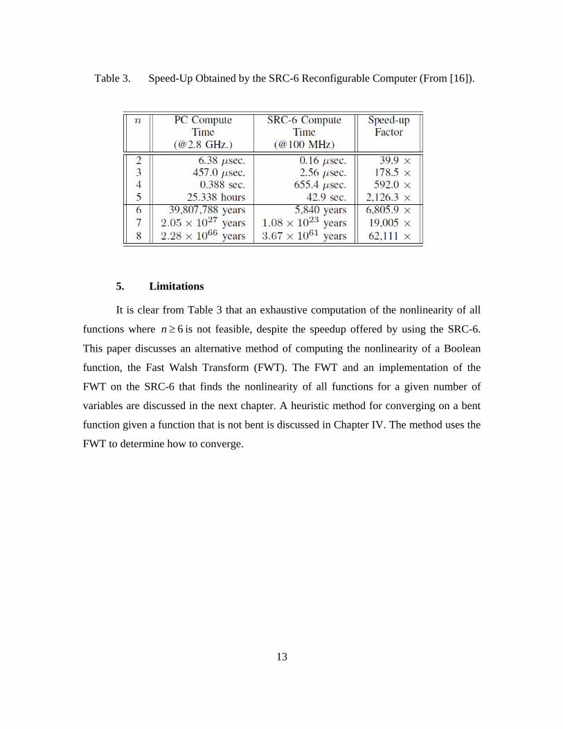
Table 3. Speed-Up Obtained by the SRC-6 Reconfigurable Computer (From [16]).
5. Limitations
It is clear from Table 3 that an exhaustive computation of the nonlinearity of all
functions where 6n is not feasible, despite the speedup offered by using the SRC-6.
This paper discusses an alternative method of computing the nonlinearity of a Boolean
function, the Fast Walsh Transform (FWT). The FWT and an implementation of the
FWT on the SRC-6 that finds the nonlinearity of all functions for a given number of
variables are discussed in the next chapter. A heuristic method for converging on a bent
function given a function that is not bent is discussed in Chapter IV. The method uses the
FWT to determine how to converge.

14
THIS PAGE INTENTIONALLY LEFT BLANK

15
III. FAST WALSH TRANSFORM
A. INTRODUCTION
Walsh-Hadamard transforms (WHTs) are recursively computed 2n by 2n matrices
that are multiplied by a vector. For n = 0, the WHT matrix is defined to be WHT0 = 1.
For greater n, the WHT matrix is defined as [17]:
1 1
1 1
1
2n n
nn n
WHT WHTWHT
WHT WHT
(1)
The factor preceding the matrix is a normalization factor. This factor is often
omitted. This matrix is then multiplied by a vector containing the TT of a function to
compute the WHT.
The fast Walsh transform (FWT) is an efficient method for computing a WHT.
The WHT has a computational complexity of n2. The FWT, on the other hand, has a
computational complexity of n log(n). This is a significant reduction in the amount of
required computations [9].
B. COMPUTATION
The FWT is a relatively simple computation. Given a valid TT, pairs of digits
from the TT are coupled and modified by an “in-place butterfly” module. Here, the term
“in-place” means that the values produced by the butterfly module output are placed in
the same position from which the butterfly module inputs came. For inputs a and b, the
outputs of the butterfly module will be a+b and a-b, respectively. An example of the
butterfly module is shown in Figure 5.

16
Figure 5. Example of In-Place Butterfly Module.
The first set of butterfly modules pairs adjacent elements and produces a 2n
element array. This process is repeated a second time, pairing every other element in the
first array to produce a second array. The third iteration will pair every fourth element in
the second array, and so on. A complete computation of the FWT of a TT with 3n is
shown in Figure 6.
Figure 6. Example of a Computation of Fast Walsh Transform.

17
C. FWT COEFFICIENT RANGES
An interesting and important observation is the value of the first element of the
FWT, which shall be referred to as FWT0. The value of FWT0 is equal to the weight of
the input TT, which is the number of ones contained in the input TT. This is always true,
since the first element of the iterations of the FWT computation always receives the left
portion of the butterfly ( )a b . Therefore, its output is the sum of all bits in the TT and
FWT0 has a range of values from zero to 2n .
The other elements of the FWT also have a range that is dependent on n. As n
increases, computation of the FWT requires more iterations. Each iteration produces
another array and expands the range of each element in the array. For example, the TT
elements only have range from 0 to 1. The first array of the FWT computation will have a
maximum value of 2 and a minimum value of 1 . The second array of the FWT
computation will have a maximum value of 4 and a minimum value of 3 . The third
array (which is the FWT in the example shown in Figure 6) will have a maximum value
of 8 and a minimum value of 7 . Generalizing this pattern, the FWT result will be the
nth array and the gth array will have a maximum value of 2g and a minimum value of
(2 1)g .
D. EXPECTED AND UNEXPECTED DISTANCE
Consider an example function f with 10011100fTT where 3n . Since there
are 8 bits in the TT of f and each bit is assumed to have an equal probability of being
either a one or a zero, we can expect that the average Hamming distance between f and
any other function with 3n to be equal to half the number of bits in the TT. This value
is referred to as the expected distance [9] to f and in this example is 2
42
n
.
Now let us consider an affine function with 3n , namely, with the truth table
01100110gTT . Computing the Hamming distance gives ( , ) 6d f g . The difference
between this Hamming distance and the expected difference is 2 and is referred to as the
unexpected distance [9]. The greater the magnitude of the unexpected difference, the

18
more bent the function is. The Hamming distances and unexpected differences between
all of the affine functions and function f are displayed below in Table 4.
Table 4. Unexpected Differences of Linear Functions From Example Function.
Linear Function Truth Table Hamming
Distance
Unexpected
Distance
1 11111111 4 0
1x 01010101 4 0
2x 00110011 6 +2
2 1x x 01100110 6 +2
3x 00001111 4 0
3 1x x 01011010 4 0
3 2x x 00111100 2 2
3 2 1x x x 01101001 6 +2
Example Function Truth Table
f 10011100
The complements of the linear functions in Table 4 are comprise the remainder of
the affine functions and are shown in Table 5. Note that the unexpected differences of the
functions in Table 5 are the negatives of those in Table 4. Therefore, it becomes
unnecessary to consider the complements of the affine functions.

19
Table 5. Unexpected Differences of the Complements of Affine Functions From Example Function.
Complements of Linear Functions Truth Table Hamming Distance Unexpected
Distance
0 00000000 4 0
1 1x 10101010 4 0
2 1x 11001100 2 2
2 1 1x x 10011001 2 2
3 1x 11110000 4 0
3 1 1x x 10100101 4 0
3 2 1x x 11000011 6 +2
3 2 1 1x x x 10010110 2 2
Example Function Truth Table
f 10011100
E. BOOLEAN FUNCTION NONLINEARITY
Consider the example function f with 10011100fTT . This function’s FWT was
computed as the example in Figure 6 and was shown to be
4 0 2 2 0 0 2 2fFWT . Recalling that FWT0 is equal to the number of ones
in the TT, we now note that the remaining digits of the FWT correspond exactly to the
magnitude and sign of the unexpected differences shown in Table 4. Thus, the FWT is an
easy way to quickly compute the unexpected difference between a function and every
affine function.

20
From the FWT it is relatively simple to determine the nonlinearity of the function.
The first step is to add 22
n to every element of the FWT except FWT0. This gives an
array of nonlinearities for both the affine functions and complements of affine functions.
Recall from Table 1 that when a function has a Hamming Distance of d from an affine
function, then that function has a Hamming Distance of 2n d from the complement of
that affine function. Since the nonlinearity of a function is found using only the smallest
of the Hamming Distances, we apply a conditional statement to each element of the array
of nonlinearities. If an element is greater than 22
n, then we subtract the nonlinearity
from 2n to get the smaller nonlinearity. If an element is less than or equal to 22
n, then no
adjustment is needed. Finally, the nonlinearity of the function is the smallest of all
adjusted elements. This process is demonstrated in Figure 7.
Figure 7. Example of a Computation of Nonlinearity From Fast Walsh Transform.

21
IV. ALGORITHM FOR BENT FUNCTION DISCOVERY
A. INTRODUCTION
Previous methods of bent function discovery, such as the sieve method described
in Chapter I, focused on exhaustive enumeration of all Boolean functions. Other studies
have attempted to overcome the difficulty in exhaustive enumeration by focusing on a
specific subset of Boolean functions [12]. By contrast, it was a primary objective of this
thesis to explore the possibility of identifying bent functions via modification of a TT that
was not bent using information from its FWT. Such a process would take the TT of a
non-bent function and produce a “nearby” function with a greater nonlinearity. For this
thesis, a “nearby” function will be defined as a function with a Hamming distance of one
from the original one. Due to the ease in computation and better demonstrability, this
thesis will consider this objective using the n = 4 case.
B. INCREASING NONLINEARITY
When the nonlinearity of a function is low, finding a nearby function with higher
nonlinearity is a relatively easy task. Taking any affine function and changing any single
bit of its TT will give a new function with a nonlinearity of one. There are (16,1) 16C
ways to change one bit, and with 32 affine functions, this gives (16)(32) = 512 functions.
As shown in Figure 8, there are 512 functions with nonlinearity of one.
Now consider the case where one modifies any two bits of an affine function’s
TT. There are (16,2) 120C ways to change two bits of an affine function’s TT. Since
there are 32 affine functions, there should be (120)(32) = 3840 functions with
nonlinearity of two. The existence of 3,840 unique functions with nonlinearity of two is
confirmed in Figure 8. Thus, changing any two bits of an affine function increases
nonlinearity by two.
One can go further and consider the case where any three bits of an affine
function’s TT are modified. Here there are (16,3) 560C ways to change three bits of an
affine function’s TT. This implies there should be (560)(32) = 17,920 functions with

22
nonlinearity of 3. The existence of 17,920 unique functions with nonlinearity of three is
also confirmed in Figure 8. Thus, changing any three bits of an affine function increases
nonlinearity by three.
Note that this pattern does not hold when considering the number of functions
with nonlinearity of four. This is because when a nonlinearity of four has been reached,
there will be a great number of functions that would be “double counted.” For example,
consider the affine function 0f and the affine function 1g x . These functions have
TTs of 0000000000000000fTT and 0101010101010101gTT , respectively. It is
possible to alter four different bits in each truth table and end up with the same function
with 0101010100000000hTT . Function h has a nonlinearity of four.
An interesting observation was made about functions with nonlinearity of five.
Note that there are exactly 16 times as many functions with nonlinearity of five as there
are bent functions. Exhaustive testing for four-variable functions showed that for every
function with nonlinearity of five, there was exactly one bit that when complemented
yielded a bent function. A change in any other bit would yield a function with
nonlinearity of four, however. This fact demonstrates that it is no longer trivial to find
nearby functions with higher nonlinearity when a function is nearly bent.

23
Figure 8. Distribution of Nonlinearity for Boolean Functions With n = 4 (From [18]).
Another distribution of four-variable functions is shown in Figure 9. This
distribution is broken down by nonlinearity and weight. This figure nicely illustrates the
ease of increasing the nonlinearity of functions that are nearly affine and the difficulty of
increasing the nonlinearity of functions that are nearly bent.
An interesting observation that can be made from Figure 9 is that complementing
any bit of any function’s truth table will produce a function with a different nonlinearity,
either higher or lower. For instance, consider the functions with a nonlinearity of three
and a weight of three. Complementing any bit of such a function produces a function with
a weight of either two or four. This will always produce a function with a nonlinearity of
two or a nonlinearity of four, because there are no functions of nonlinearity three with a
weight of two or four. This pattern holds for all functions of any nonlinearity or weight.

24
Consider a function with a nonlinearity of two and weight of two. It is trivial to
find a nearby function with increased nonlinearity. Complementing any 0 bit in this
function’s truth table will produce a function with nonlinearity of three and weight of
three. Note that it is impossible to do this and receive a function with lower nonlinearity,
since there are no functions with a nonlinearity of one and weight of three for n = 4.
Now consider a function with a nonlinearity of five and weight of five. As shown
by Figure 9, there are 2,688 such functions. In order to have a bent function, the weight
must be increased by one since all bent functions have weight of six or ten. However,
increasing the weight is far more likely to actually decrease the nonlinearity. Note that for
a weight of six, there are exactly fifteen times more functions with nonlinearity of four
(6,720) than there are with nonlinearity of six (448).
Figure 9. Distribution of Four-Variable Functions Over Nonlinearity and Weight (From [18]).

25
This may not seem particularly problematic, as using a trial-and-error method to
determine which bit to change to go from a nonlinearity of five to a nonlinearity of six
will take at most 16 attempts. However, the amount of potential attempts grows
exponentially as n increases, as there are 2n bits in a TT. In addition, each attempt entails
a computation of a function’s nonlinearity in order to determine if the trial was successful
or not. Recall that using the sieve method to compute the nonlinearity may take many
clock cycles, and using the FWT to compute the nonlinearity takes multiple clock cycles
as well. In addition, as n increases, the number of clock cycles required to compute the
nonlinearity via the sieve method or by the FWT increases as well. Clearly, a trial-and-
error method to produce a bent function is not a fast process.
In order to reduce the number of amount of time needed to find a nearby function
with higher nonlinearity, we will use characteristics of the FWT to immediately eliminate
many potential bit changes and greatly speed up discovery of bent functions.
C. FWT SPECTRUM CHARACTERISTICS
An exhaustive examination of the FWTs of Boolean functions with 4n
revealed interesting information about the composition of FWTs. For each nonlinearity, a
FWT always consisted of a specific set of values (except for the FWT0 term, which is
simply the function’s weight). The FWT of a bent function with nonlinearity of six
always consisted only of values of 2 and 2 . The FWT of a function with nonlinearity of
five always consisted only of values contained in the set { 3 , 1 ,1,3}. Likewise, the
FWT of a function with nonlinearity of four always consisted only of values contained in
the set { 4 , 2 ,0,2,4}. FWTs for functions with nonlinearities of three, two, one, and
zero all have specific sets of values as well. These observations are shown in Table 6.
The placement of these values throughout the FWT varies with the function being
considered, but the values present in the FWT are affected only by the function’s
nonlinearity. This trait was also noted in limited observation of functions with n = 6, but
due to our inability to exhaustively test the FWTs of these functions, this thesis will focus
on the n = 4 case.

26
Table 6. Possible Values Contained in FWT Elements for Various Nonlinearities for n = 4.
Nonlinearity Possible Values Contained in FWT Elements (Except FWT0)
6 2 , 2
5 3 , 1 , 1, 3
4 4 , 2 , 0, 2, 4
3 5 , 3 , 1 , 1, 3, 5
2 6 , 2 , 0, 2, 6
1 7 , 1 , 1, 7
0 8 , 0, 8
D. EFFECT OF TRUTH TABLE CHANGES ON FWT
It has already been established that changing a 0 bit to a 1 bit in a given TT
increments the value of FWT0 by one. An interesting question was whether or not the
values of the other elements of the FWT could also be predictably altered by a change in
the function’s TT. It was discovered that one can indeed predict the change in any
element of a FWT caused by a change in the function’s TT.
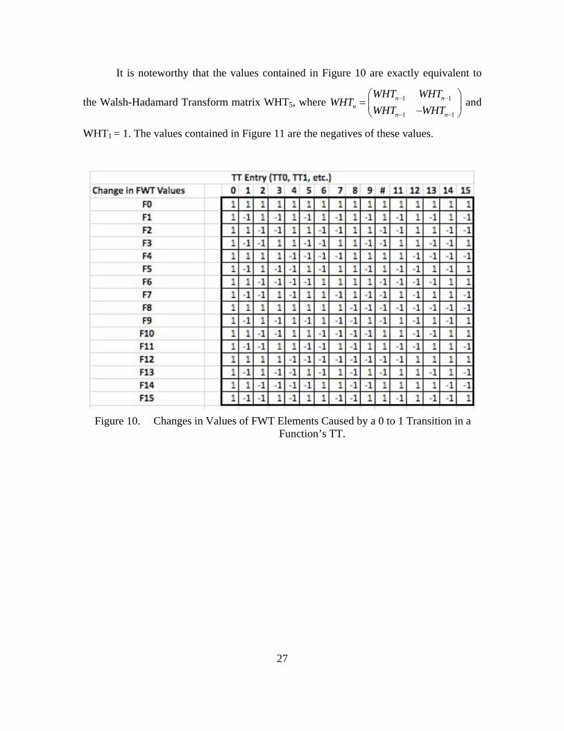
Exhaustive testing showed the derivation of the values shown in Figure 10 and
Figure 11. The effects on each element of the FWT due to a 0 to 1 transition in any TT
element and due to a 1 to 0 transition in any TT element, respectively, are shown. For
example, if one were to change TT5 from a zero to a one, FWT0 will increase by one,
FWT1 will decrease by one, FWT2 will increase by one, and so on. If one were to change
TT6 from a 1 to a 0, FWT0 will decrease by one, FWT1 will decrease by one, FWT2 will
increase by one, FWT3 would increase by one, and so on.
27
It is noteworthy that the values contained in Figure 10 are exactly equivalent to
the Walsh-Hadamard Transform matrix WHT5, where 1 1
1 1
n nn
n n
WHT WHTWHT
WHT WHT
and
WHT1 = 1. The values contained in Figure 11 are the negatives of these values.
Figure 10. Changes in Values of FWT Elements Caused by a 0 to 1 Transition in a Function’s TT.
28
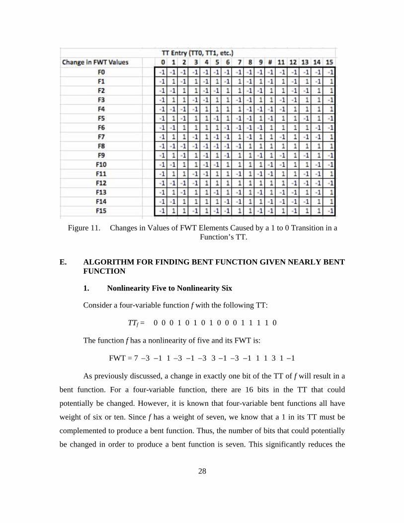
Figure 11. Changes in Values of FWT Elements Caused by a 1 to 0 Transition in a Function’s TT.
E. ALGORITHM FOR FINDING BENT FUNCTION GIVEN NEARLY BENT FUNCTION
1. Nonlinearity Five to Nonlinearity Six
Consider a four-variable function f with the following TT:
TTf = 0 0 0 1 0 1 0 1 0 0 0 1 1 1 1 0
The function f has a nonlinearity of five and its FWT is:
FWT = 7 3 1 1 3 1 3 3 1 3 1 1 1 3 1 1
As previously discussed, a change in exactly one bit of the TT of f will result in a
bent function. For a four-variable function, there are 16 bits in the TT that could
potentially be changed. However, it is known that four-variable bent functions all have
weight of six or ten. Since f has a weight of seven, we know that a 1 in its TT must be
complemented to produce a bent function. Thus, the number of bits that could potentially
be changed in order to produce a bent function is seven. This significantly reduces the

29
number of bits that would potentially need to be tested in a trial-and-error technique.
However, for functions with higher values of n, this can still result in a large number of
bits to be tested.
A method for reducing the number of bits even further is to consider the contents
of the FWT of f. Note that the FWT (except FWT0) contains values 3 , 1 , 1, and 3.
This is the set of values that are potentially present in the FWT of a function with
nonlinearity of five. Recall that a bent function’s FWT will only contain values 2 and 2
and a function with nonlinearity of four will potentially have values 4 , 2 , 0, 2, and 4.
If the incorrect TT bit is chosen to be complemented, then one or more of the FWT
components with values 3 or 3 will become 4 or 4, respectively. This would produce a
function with a lower nonlinearity. For example, consider if we (incorrectly) choose to
complement the first 1 bit in the TT. This bit is referred to as TT3 in Figures 10 and 11.
From Figure 11, it can be seen that changing TT3 from a 1 to a 0 will decrease the value
of FWT4 by one and will increase the value of FWT13 by one. This would make FWT4
equal to 4 and FWT13 equal to 4. This indicates a function with a nonlinearity of four
without having to recalculate the nonlinearity of the new function that was produced. The
TT and FWT resulting from this incorrect transition are:
Tg = 0 0 0 0 0 1 0 1 0 0 0 1 1 1 1 0 (2)
and
WT = 6 2 0 0 4 0 2 2 2 2 0 0 0 4 2 2 . (3)
As another example, consider if we (correctly) choose to complement TT5. Doing
so will cause all FWT values that had been 3 to become 2 and all FWT values that had
been 3 to become 2. This produces a bent function with nonlinearity of six. The TT and
FWT resulting from this correct transition are:
Th = 0 0 1 0 0 0 1 0 0 0 1 1 1 1 0 (4)
and
WT = 6 2 2 2 2 2 2 2 2 2 2 2 2 2 2 2 . (5)

30
A flowchart that describes this algorithm is shown in Figure 12.
Figure 12. Algorithm for Finding Bent Function Given Four-Variable Function With Nonlinearity of Five.

31
2. Nonlinearity Four to Nonlinearity Five
The algorithm for altering a function with nonlinearity four to produce a function
with nonlinearity five is quite similar to the algorithm just described. The major
difference in this case is that for functions with certain weights we are not forced to
complement a 1 or complement a 0. For example, a function with weight of four must
have its weight increased by one by complementing a 0 bit. Conversely, a function with
weight of twelve must have its weight decreased by one by complementing a 1 bit. For
functions with weight of six, eight, or ten, we can either decrease or increase the weight
to produce a function with nonlinearity of five.
Consider a function f with nonlinearity of four and the following TT and FWT:
Tf = 0 0 0 1 0 0 1 0 0 0 1 1 1 1 0; (6)
WT = 6 0 0 2 4 2 2 0 2 0 0 2 0 2 2 4 . (7)
Note that the FWT of this function contains the proper values for a function with
nonlinearity of four. In order to produce a function with nonlinearity of five, a TT
transition that forces both of the FWT values of 4 to become 3 is necessary. Because
the function has weight of six, we can either complement a 0 bit or a 1 bit. Arbitrarily
choosing to complement a 0 bit, we see from Figure 11 that complementing TT0
increases both FWT5 and FWT15 (and actually, changing TT0 from 0 to 1 will increase
every element of the FWT). Choosing to complement this bit produces a function g of
nonlinearity five with the following TT and FWT:
Tg = 1 0 0 0 1 0 0 1 0 0 0 1 1 1 1 0; (8)
WT = 7 1 1 3 3 1 1 1 1 1 1 3 1 3 3 3 . (9)
A flowchart that describes this algorithm is shown in Figure 13. The output of this
algorithm could then be the input to the algorithm shown in Figure 12, which would
produce a bent function.
The algorithm for altering any function with nonlinearity of less than four in order
to produce a function with greater nonlinearity is similar to this algorithm.

32
Figure 13. Algorithm for Finding a Function With Nonlinearity of Five Given a Four-Variable Function With Nonlinearity of Four.

33
V. COMPUTATION AND ANALYSIS
A. IMPLEMENTATION OF FWT ON SRC-6
1. About the SRC-6
The SRC-6 reconfigurable computer in Spanagel Hall at the Naval Postgraduate
School is the one of the computational tools used for this thesis. The SRC-6 allows the
user greater flexibility to control compilation than a PC. It is composed of two PCs, each
with a Pentium IV microprocessor, five Multi-Adaptive Processing (MAP) boards each
containing three Xilinx Virtex-2 XC2V6000 FPGAs, two for computing and one for
control as well, as well as 24 MB of On Board Memory (OBM). A high-bar switch
connects these components. These boards are connected by a high-bar switch. The SRC-6
has four 8 GB banks of common memory. The SNAP port can send data from the
microprocessor to the MAP at a maximum speed of 1400 MB/s. A diagram of the SRC-6
is shown in Figure 14.
Figure 14. Layout of the SRC-6 (From [15]).

34
Several files are required to execute a program on the SRC-6. The SRC-6 can
compile code that can be either executed on the Intel processor or on the MAP. The files
are linked together in order to create a single executable. Files that are Intel targeted are
compiled to an .o file and files that are targeted to the MAP compile using the Map C
Compiler (MCC). The file main.c is written in C and calls a subroutine file which does
the bulk of the computation. The file main.c is typically used to format and display the
output and sends inputs to the subroutine. The file subr.mc is the subroutine that main.c
calls. It is also written in C and runs on the MAP. The subroutine subr.mc can call built-
in or user-created macros. Local memory and On Board Memory (OBM) are used for
data storage. The SRC-6 contains six OBM banks. Each OBM bank is capable of storing
523,776 64-bit words. The SRC-6 FPGA contains 144 Block RAM (BRAM) units. Each
BRAM unit is capable of storing 2048 bytes. BRAM units can conduct a read and a write
simultaneously.
The user can define macros on the SRC-6. Macros are written using VERILOG or
VHDL and define the circuits generated on the FPGA. The macro is the module that
performs the desired computations, and it can be called millions of times by the
subroutine. Users can pipeline the macro so that it can perform one computation each
clock cycle. This significantly boosts throughput when compared to a PC. This is usually
where the major computations occur. The macro can be called millions of times in the
subroutine. It can be pipelined to increase throughput, a major advantage over a PC.
Macros require several files to operate: a blk.v file that acts as a black box and specifies
inputs and outputs of the macro and an info file that describes the characteristics of the
inputs and outputs as well as the characteristics of the macro.
2. Use of the SRC-6
It was exceptionally useful utilizing the SRC-6 for computing the nonlinearity of
millions of functions. The subroutine used a counter in order to exhaustively test all
functions for a given n. Each function generated by the counter was sent to the macro as
an input to be tested. The function was tested for its nonlinearity by utilizing its FWT.

35
The values of functions’ nonlinearities were sent back to the subroutine and stored in a
histogram. The histogram counted the number of functions with each nonlinearity.
In addition to exhaustively computing the nonlinearities of functions by using the
FWT, the nonlinearities were also computed separately by an implementation of the sieve
technique. This was done so as to obtain a comparison against a benchmark in order to
ascertain the feasibility of computing the FWT on the SRC-6.
3. Limitations of the SRC-6
The primary limitation of the SRC-6 is the speed of its FPGA. The SRC-6 runs at
100 MHz, so a limit of 100,000,000 functions can be tested each second. Due to this, it is
impractical to exhaustively test all function with more than five variables. Computing the
nonlinearity of every six variable function, for example, would take about 62
1121.85 10 sec 5,845
100
functionsx years
MHz . Due to this limitation, only limited numbers
of computations were performed for six-variable functions.
Another limitation of the SRC-6 is the inability to compile designs that require
more than 10 ns between clock cycles. This can occur when a program requires extensive
computations or it is written inefficiently. This can be encountered sometimes in Verilog
while using behavioral code. Behavioral code involves the use of loops, conditionals, and
calls to functions. A more efficient method of coding on the FPGA is to use structural
code. Structural code involves the use of wire connections that perform simple operations
synchronized with the edge of a clock pulse or the change of an input quantity. Structural
code includes the use of registers, which can be used to store and recall information on a
clock pulse. This allows pipelining code, which can significantly lower the time between
cycles and allow a program to compile properly.
A final limitation of the SRC-6 is that its FPGA has a limited amount of space
available for hardware design. With more variables in a function, the larger the circuit
required to compute its nonlinearity becomes. As n increases to approximately nine or
ten, the FPGA’s resources are no longer sufficient to construct the specified circuit. It is

36
conceivable to use a second FPGA to add the required resources to construct circuits for
high values of n, but this has not been explored.
B. RESULTS AND ANALYSIS OF IMPLEMENTATION OF FWT ON THE SRC-6
1. Nonlinearity for n = 4
For the 216 four-variable functions, the nonlinearities were computed for each of
these using the FWT method, a pipelined FWT method, as well as the sieve method for a
comparison. A summary of the relevant performance metric is shown in Table 7. All
methods were able to be compiled on the SRC-6, as their frequencies were all greater
than 100 MHz. The methods, as expected for a small value of n, all use a similarly small
amount of the FPGA’s resources. It is of note that the pipelined FWT method executes
most quickly, with a frequency of 110 MHz. The distribution of nonlinearities obtained
with the FWT methods is shown in Figure 15 and precisely matches the distribution
shown in Figure 9, confirming that the FWT method correctly computed the nonlinearity
for all functions.
Table 7. Comparison of Methods for n = 4.
Sieve Method FWT Method Pipelined FWT
# Clock Cycles 65,727 65,737 65,737
Latency (clock
cycles)
6 16 18
# LUTs Used (%) 3,717 (4%) 3,923 (4%) 4,012 (4%)
Frequency (MHz) 101.0 100.2 110.0

37
Figure 15. Distribution of Functions With Four Variables by Nonlinearity.
2. Nonlinearity for n = 5
For the 232 five-variable functions, the nonlinearities were computed for each
using the FWT method, a pipelined FWT method, as well as the sieve method for a
comparison. A summary of the relevant performance metric is shown in Table 8. The
sieve method and the pipelined FWT were able to be compiled and run on the SRC-6, as
their frequencies were greater than 100 MHz. Note that in this case, the sieve method
runs faster than the pipelined FWT. In addition, the latency of the pipelined FWT is much
higher than the latency of the sieve method. This is conjectured to be due to the circuit
having exponential complexity in n, where complexity is shown by the number of LUTs
used. The distribution of nonlinearities for n = 5 is shown in Figure 16. Approximately
0.64% of the functions have maximum nonlinearity, which is about half of the proportion
of bent functions that exist for n = 4.

38
Table 8. Comparison of Methods for n = 5.
Sieve Method FWT Method Pipelined FWT
# Clock Cycles 4,294,967,488 4,294,967,513 4,294,967,513
Latency (clock
cycles)
7 32 34
# LUTs Used (%) 3969 (4%) 5,134 (5%) 5,511 (6%)
Frequency (MHz) 111.8 78.6 100.0
Figure 16. Distribution of Functions With Five Variables by Nonlinearity.
3. Nonlinearity for n = 6
Since it was not possible to compute the nonlinearities of all 264 functions with six
variables, we rather computed the nonlinearity for a subset of 232 of them. For these
functions, the nonlinearities were computed for each using the FWT method, a pipelined
FWT method, as well as the sieve method for a comparison. A summary of the relevant

39
performance metric is shown in Table 9. The sieve method and the pipelined FWT were
able to be compiled and run on the SRC-6, as their frequencies were greater than 100
MHz. The non-pipelined FWT method suffered a sharp drop-off in frequency. In
addition, the latency of the pipelined FWT is much higher than the latency of the sieve
method and seems to be growing exponentially.
Table 9. Comparison of Methods for n = 6.
Sieve Method FWT Method Pipelined FWT
# Clock Cycles 4,294,967,489 4,294,967,545 4,294,967,545
Latency (clock
cycles)
8 64 67
# LUTs Used (%) 4,486 (5%) 8,615 (9%) 9,269 (10%)
Frequency (MHz) 102.1 48.3 100.1
4. Trends of Performance Metrics
The trends of the frequency and resource usage for the nonlinearity computation
methods are shown for increasing n in Figure 17. It becomes clear that the FWT method,
without pipelining, will not compile for n greater than five. A pipelined version of the
FWT method, however, performs much better. The pipelined FWT method and the sieve
method share roughly equivalent execution frequencies up to about an n of ten.

40
Figure 17. Trend of Frequency for Nonlinearity Computation Methods for Various n.
The total number of four-input Lookup Tables (LUTs) used is shown in Figure
18. A LUT is the key type of data structure used in FPGAs. An n-bit LUT can encode any
n-bit Boolean function by modeling it as a truth table. LUTs are, therefore, a very
efficient method for encoding Boolean logic functions.
One aspect where the FWT method is decidedly less desirable than the sieve
method is in the amount of resources it used. The number of LUTs used by the sieve
method increased almost linearly with n. The number of LUTs used by the FWT method,
on the other hand, increased roughly exponentially with n. The FPGA in the SRC-6
contains 88,192 four-input LUTs. The amount of resources available on the SRC-6 would
allow use of the SRC-6 method for n up to nine. It would be conceivable to use a second
FPGA for higher n, but this has not been attempted.

41
Figure 18. Trend of Resource Utilization for Nonlinearity Computation Methods for Various n.
C. IMPLEMENTATION OF ALGORITHM ON PC USING MATLAB
MATLAB was used to write code to implement the algorithm described in
Chapter IV. This algorithm was used for the n = 4 case, but can be expanded for use with
higher n. The algorithm takes a TT and n as inputs and returns the TT of a nearby
function with higher nonlinearity if one exists. The range of input TT accepted in this
implementation was limited to those with a nonlinearity of three or greater. This is
because of the ease in finding functions with nonlinearity four or greater, as discussed in
Chapter IV.
This algorithm was performed on all functions with a nonlinearity of three, four,
five, and six. It always chose a bit that, when complemented, produced a nearby function
with greater nonlinearity if such a function existed. An example of the output from this
implementation is shown in Figure 19.

42
Figure 19. Sample Output of Algorithm That Discovers Nearby Bent Functions.
The algorithm was applied to every four-variable function. Input functions with
nonlinearity less than three were ignored. The inputs were filtered so that the algorithm
was performed separately on functions with starting nonlinearities of three, four, and five.
For example, the algorithm was applied to all 17,920 functions with a nonlinearity
of three. This produced a certain number of functions with a nonlinearity of four, on
which the algorithm was applied again. This produced a certain number of functions with
a nonlinearity of five, on which the algorithm was applied again. This produced a certain
number of bent functions.
After this, the algorithm was applied to all 28,000 functions with a nonlinearity of
four. This produced a certain number of functions with a nonlinearity of five on which
the algorithm was applied once more. This then produced bent functions.
43
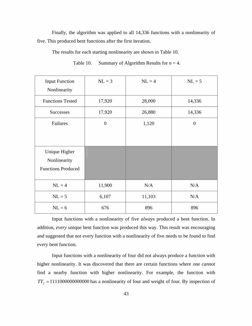
Finally, the algorithm was applied to all 14,336 functions with a nonlinearity of
five. This produced bent functions after the first iteration.
The results for each starting nonlinearity are shown in Table 10.
Table 10. Summary of Algorithm Results for n = 4.
Input Function
Nonlinearity
NL = 3 NL = 4 NL = 5
Functions Tested 17,920 28,000 14,336
Successes 17,920 26,880 14,336
Failures 0 1,120 0
Unique Higher
Nonlinearity
Functions Produced
NL = 4 11,900 N/A N/A
NL = 5 6,107 11,103 N/A
NL = 6 676 896 896
Input functions with a nonlinearity of five always produced a bent function. In
addition, every unique bent function was produced this way. This result was encouraging
and suggested that not every function with a nonlinearity of five needs to be found to find
every bent function.
Input functions with a nonlinearity of four did not always produce a function with
higher nonlinearity. It was discovered that there are certain functions where one cannot
find a nearby function with higher nonlinearity. For example, the function with
1111000000000000fTT has a nonlinearity of four and weight of four. By inspection of

44
Figure 9, we know that complementing a 1 bit from its TT will decrease its weight and
nonlinearity to three. However, it turns out that complementing any of its 0 bits will
produce a function with a weight of five and a nonlinearity of three.
There were 1,120 input functions with a nonlinearity of four for which it was not
possible to find a nearby function with nonlinearity of five. Every other input function
with a nonlinearity of four, however, produced a nearby function with a nonlinearity of
five. This produced a total of 11,103 unique functions with a nonlinearity of five. From
those unique functions, the algorithm was then able to find all 896 bent functions. It is
particularly noteworthy that not all functions with a nonlinearity of five need to be
discovered in order to discover all the bent functions.
Input functions with a nonlinearity of three always produced a function with a
nonlinearity of four. This produced a total of 11,900 unique functions with a nonlinearity
of four. From the functions produced that had a nonlinearity of four, the algorithm was
able to produce 6,107 unique functions with a nonlinearity of five. From these functions,
676 unique bent functions were produced.

45
VI. CONCLUSIONS AND RECOMMENDATIONS
A. CONCLUSIONS
An SRC-6 implementation of the FWT method for computing the nonlinearity of
all functions of a given n was accomplished in this thesis. This method had an execution
frequency that was comparable with the method by which the Hamming distance from
each affine function is computed and the minimum Hamming distance is taken. As with
other methods that exhaustively compute the nonlinearity of functions in order to
discover bent functions, the feasibility of this method was limited by the number of
variables in the input functions. The FWT method requires more 4-input LUTs than are
available one FPGA on the SRC-6 once n ≥ 10.
An algorithm that uses information from the FWT of an input function to produce
a “nearby” function with higher linearity was also accomplished in this thesis. When a
nearby function with higher nonlinearity exists, the algorithm always is able to find it.
Instead of having to compute the nonlinearity of 22n
functions in order to find every bent
function, it was possible to apply the algorithm to a smaller set of functions and find
every bent function. For example, for n = 4 there are 28,000 functions with a nonlinearity
of four. This represents only 43% of all four-variable functions. From this smaller set of
functions the algorithm was able to produce every bent function.
Included in the Appendices are several sets of code that may aid those who chose
to continue this research in the future.
B. RECOMMENDATIONS
There are several ideas that may improve or expand upon the work done in this
thesis. There are several options available that may enhance the effectiveness of the SRC-
6. The SRC-6 contains two programmable FPGAs on each MAP. Only one FPGA was
used in the implementation of the code in this thesis. Using the second FPGA may allow
the computation of nonlinearities of functions with n ≥ 10. A potential pitfall is that only
one 64-bit value can be passed to and from an FPGA at a time. The TT of a 12-variable

46
function contains 4096 bits, thus it would be necessary to pass 64 different 64-bit values
between FPGAs to send the TT to the second FPGA. Since the FWT contains values
other than 1 and 0, it contains many more bits than the TT. This would be even more
difficult to pass between two FPGAs. This could potentially slow pipelining of the FWT
method substantially.
Another idea that may provide useful results would be to use the algorithm
developed in this thesis in conjunction with previous research. Specifically, Shafer’s
work that identified groups of Boolean functions that were rich in bent functions [12]. It
was demonstrated in this thesis that it is possible to find all bent functions by using a
subset of all functions. It may be possible to find all bent functions for higher n by
adapting the algorithm for higher n and applying it to certain sets of functions with
specific degree, rotational symmetry, homogeneity, or other criteria.
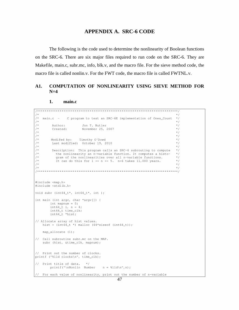
47
APPENDIX A. SRC-6 CODE
The following is the code used to determine the nonlinearity of Boolean functions
on the SRC-6. There are six major files required to run code on the SRC-6. They are
Makefile, main.c, subr.mc, info, blk.v, and the macro file. For the sieve method code, the
macro file is called nonlin.v. For the FWT code, the macro file is called FWTNL.v.
A1. COMPUTATION OF NONLINEARITY USING SIEVE METHOD FOR N=4
1. main.c
/***************************************************************************/ /* */ /* main.c - C program to test an SRC-6E implementation of Ones_Count */ /* */ /* Author: Jon T. Butler */ /* Created: November 25, 2007 */ /* */ /* */ /* Modifed by: Timothy O'Dowd */ /* Last modified: October 19, 2010 */ /* */ /* Description: This program calls an SRC-6 subrouting to compute */ /* the nonlinearity an n-variable function. It computes a histo- */ /* gram of the nonlinearities over all n-variable functions. */ /* It can do this for 1 <= n <= 5. n=6 takes 11,000 years. */ /* */ /* */ /***************************************************************************/ #include <map.h> #include <stdlib.h> void subr (int64_t*, int64_t*, int ); int main (int argc, char *argv[]) { int mapnum = 0; int64_t i, n = 4; int64_t time_clk; int64_t *hist; // Allocate array of hist values. hist = (int64_t *) malloc (64*sizeof (int64_t)); map_allocate (1); // Call subroutine subr.mc on the MAP. subr (hist, &time_clk, mapnum); // Print out the number of clocks. printf ("%lld clocks\n", time_clk); // Print title of data. */ printf("\nNonlin Number n = %lld\n",n); // For each value of nonlinearity, print out the number of n-variable

48
// functions with that nonlinearity. for (i = 0; i <= (1<<n); i++){ printf(" %lld %lld \n",i, hist[i]); }//for (i = 0; i <= (1<<2); i++){ map_free (1); exit(0); }//int main (int argc, char *argv[]) {
2. subr.mc
/***************************************************************************/ /* */ /* subr.mc - MAP C subroutine to compute the nonlinearity of functions. */ /* */ /* Author: Jon T. Butler */ /* Created: November 25, 2007 */ /* */ /* */ /* Modified by: Timothy O'Dowd */ /* Last modified: October 19, 2010 */ /* */ /* Description: This program calls an SRC-6 macro that computes */ /* the nonlinearity an n-variable function. It computes a histo- */ /* gram of the nonlinearities over all n-variable functions. */ /* It can do this for 1 <= n <= 5. n=6 takes 11,000 years. */ /* */ /* */ /***************************************************************************/ #include <libmap.h> void subr (int64_t histogram[], int64_t *time, int mapnum) { // Declare an OBM bank in SRC-6 to store the histogram of nonlinearities // for n-variable functions. For n-variable functions, there are 2^n+1 // potential nonlinearities. When n=5, there are 33 nonlinearities. OBM_BANK_A (Hist, int64_t, 64) // int64_t t0, t1; int64_t sel, i, N, n = 4; int64_t my64bit_in; int64_t my64bit_out; int64_t Hist0[64], Hist1[64], Hist2[64], Hist3[64]; read_timer(&t0); // for (i = 0; i < 64; i++){ Hist0[i] = 0; Hist1[i] = 0; Hist2[i] = 0; Hist3[i] = 0; } // if (n < 5) N = 1<<(1<<n); //Form N = 2^(2^n); else N = 0x100000000; // #pragma loop noloop_dep //To avoid loop slowdown, separate histogram into // four separate histograms. for (i = 0; i < N; i++){

49
my64bit_in = i; my_operator (my64bit_in, &my64bit_out); sel = i & 3; if (sel == 0) Hist0[my64bit_out]++; if (sel == 1) Hist1[my64bit_out]++; if (sel == 2) Hist2[my64bit_out]++; if (sel == 3) Hist3[my64bit_out]++; }//for (i = 0; i < N; i++){ // for (i = 0; i < 64; i++) Hist[i] = Hist0[i] + Hist1[i] + Hist2[i] + Hist3[i]; read_timer(&t1); *time = (t1 - t0); // Return histogram to main.c DMA_CPU (OBM2CM, Hist, MAP_OBM_stripe(1,"A"), histogram, 1, 64*sizeof(int64_t), 0); wait_DMA (0); }//subr (int64_t hist[], int64_t *time, int mapnum) {
3. Makefile
# $Id: Makefile.template,v 1.13 2005/04/12 19:18:30 jls Exp $ # # Copyright 2003 SRC Computers, Inc. All Rights Reserved. # # Manufactured in the United States of America. # # SRC Computers, Inc. # 4240 N Nevada Avenue # Colorado Springs, CO 80907 # (v) (719) 262-0213 # (f) (719) 262-0223 # # No permission has been granted to distribute this software # without the express permission of SRC Computers, Inc. # # This program is distributed WITHOUT ANY WARRANTY OF ANY KIND. # # ----------------------------------- # ---------------------------------- # User defines FILES, MAPFILES, and BIN here # ---------------------------------- FILES = main.c MAPFILES = subr.mc BIN = main # ---------------------------------- # Multi chip info provided here # (Leave commented out if not used) # ---------------------------------- #PRIMARY = <primary file 1> <primary file 2> #SECONDARY = <secondary file 1> <secondary file 2> #CHIP2 = <file to compile to user chip 2> #----------------------------------- # User defined directory of code routines # that are to be inlined

50
#------------------------------------ #INLINEDIR = # ----------------------------------- # User defined macros info supplied here # # (Leave commented out if not used) # ----------------------------------- MACROS = my_macro/nonlin.v MY_BLKBOX = my_macro/blk.v MY_NGO_DIR = my_macro MY_INFO = my_macro/info # ----------------------------------- # Floating point macros selection # ----------------------------------- #FPMODE = SRC_IEEE_V1 # Default SRC version IEEE #FPMODE = SRC_IEEE_V2 # Size reduced SRC IEEE with # special rounding mode # ----------------------------------- # User supplied MCC and MFTN flags # ----------------------------------- MY_MCCFLAGS = -v -keep MY_MFTNFLAGS = -v # ----------------------------------- # User supplied flags for C & Fortran compilers # ----------------------------------- CC = gcc # icc for Intel cc for Gnu FC = ifort # ifort for Intel f77 for Gnu #LD = ifort -nofor_main # for mixed C and Fortran, main in C #LD = ifort # for Fortran or C/Fortran mixed, main in Fortran LD = gcc # for C codes MY_CFLAGS = MY_FFLAGS = MY_LDFLAGS = # Flags to include libs if needed # ----------------------------------- # VCS simulation settings # (Set as needed, otherwise just leave commented out) # ----------------------------------- #USEVCS = yes # YES or yes to use vcs instead of vcsi #VCSDUMP = yes # YES or yes to generate vcd+ trace dump # ----------------------------------- # MODELSIM simulation settings # (Set as needed, otherwise just leave commented out) # ----------------------------------- #USEMDL = yes # YES or yes to use modelsim instead of vcs/vcsi #USEMDLGUI = yes # YES or yes to use modelsim GUI interface #MDLDUMP = yes # YES or yes to generate vcd trace dump # ----------------------------------- # No modifications are required below # ----------------------------------- MAKIN ?= $(MC_ROOT)/opt/srcci/comp/lib/AppRules.make include $(MAKIN)

51
4. blk.v
/***************************************************************************/ /* */ /* blk.v - black-box file that specifies input and output */ /* */ /* Author: Timothy O'Dowd */ /* Created: July 1, 2010 */ /* Last modified: October 3, 2010 */ /* */ /***************************************************************************/ module nonlin(TT_p,nl_p,CLK); input [63:0] TT_p; output [63:0] nl_p; input CLK; endmodule
5. Info File
//***************************************************************************/ //* */ //* info - info file to specify the input and output of the macro. */ //* */ //* Author: Jon T. Butler */ //* Created: November 25, 2007 */ //* */ //* Modified by: Timothy O'Dowd */ //* Last modified: October 3, 2010 */ //* */ //***************************************************************************/ BEGIN_DEF "my_operator" //Name used in .mc file to call macro. MACRO = "nonlin"; //Macro name. STATEFUL = NO; EXTERNAL = NO; PIPELINED = YES; //n = 2 3 4 5 6 7 LATENCY = 8; //LATENCY = 4 5 6 7 8 9 INPUTS = 1: I0 = INT 64 BITS (TT_p[63:0]) // Input TT_p explicit input ; OUTPUTS = 1: O0 = INT 64 BITS (nl_p[63:0]) // Output nl_p explicit output ; IN_SIGNAL : 1 BITS "CLK" = "CLOCK"; DEBUG_HEADER = # void my_operator__dbg (int64_t TT_p, int64_t *nl_p); #; DEBUG_FUNC = # void my_operator__dbg (int64_t TT_p, int64_t *nl_p){ *nl_p = 6; } #; END_DEF

52
6. nonlin.v
///////////////////////////////////////////////////////////////////////////////////////// module nl_mapper (TT, OUT); //--------------------------------------------------------------------------------------- // nl_mapper - Verilog code to convert the truth table TT of a given function f into a // vector, OUT of 2^(n+1) functions - each with 2^n bits - that are the // distance vectors between f and the 2^(n+1) affine functions. These are // then applied to a ones_count circuit to count the number of 1's, which // are compared to find the minimum distance from f to an affine function. // // Created: November 6, 2007 // Last Modified: November 26, 2007 // Author: Jon T. Butler // // Inputs: TT //Truth table of given function, f. // Outputs: OUT //Vector of 2^(n+1) distances between f and an affine function/ // //--------------------------------------------------------------------------------------- //; parameter n = 4; // n = the number of variables. localparam N = 2**n; localparam NN = 2**(n+1); input [N-1 : 0] TT; output [N*NN - 1 : 0] OUT; reg [N*NN - 1 : 0] OUT; reg [n : 0] Y; reg [n-1 : 0] X; reg temp; integer i,j,k; always @(TT) for (i = 0; i < NN; i = i + 1) //Enumerates the affine functions. begin Y = i; for (j = 0; j < N; j = j + 1) //Enumerates the truth table entries. begin X = j; temp = 0; for (k = 0; k < n; k = k + 1) //Exclusive OR the affine function with f. temp = temp ^ (X[k] & Y[k]); OUT[Y*N + X] = temp ^ TT[X] ^ Y[n]; end end // // In the innermost for loop, we are exclusive-ORing across the variables involved // in the affine function and the function value itself - TT[X]. Here, Y[k] // determines whether a particular variable X[k] is involved (Y[k] = 1) or not (= 0). // temp is the running exclusive OR. // Y[NN-1] determines whether the affine function is linear (Y[NN-1]=0) or the complement // of a linear function (=1). endmodule ///////////////////////////////////////////////////////////////////////////////////////// module min(IN, OUT, CLK); //--------------------------------------------------------------------------------------- // min.v - A program to compare 2^(n+1) n+1-bit binary values and to deliver the // smallest to the output. This can be configured in two ways // 1. Completely pipelined tree // 2. Completely combinational tree (except for a register at the output) // // In the case of 1. this runs a 209.6 MHz. for all values of n. It was // tried for n up to 8. At n=8, it takes more than two minutes to compile.

53
// // In the case of 2. the Freq. value is as follows // // n Freq. (MHz.) Total Runtime // 2 111.9 // 3 106.1 // 4 73.6 // 5 70.4 // 6 61.2 // 7 53.2 2 min. 45 secs. // 8 46.7 7 min. 57 secs. // // To have a 1. Completely pipelined tree, use <= in three places // 1. curr_IN[0] <= IN; // ....................................... // 2. if(curr_IN[j-1][((2*i + 2)*nn-1)-:nn] < // curr_IN[j-1][((2*i + 1)*nn-1)-:nn]) // curr_IN[j][((i + 1)*nn-1)-:nn] <= // curr_IN[j-1][((2*i + 2)*nn-1)-:nn]; // ....................................... // 3. else curr_IN[j][((i + 1)*nn-1)-:nn] <= // curr_IN[j-1][((2*i + 1)*nn-1)-:nn]; // ....................................... // To have a 2. Completely combinational tree, use <= in three places // 1. curr_IN[0] = IN; // ....................................... // 2. if(curr_IN[j-1][((2*i + 2)*nn-1)-:nn] < // curr_IN[j-1][((2*i + 1)*nn-1)-:nn]) // curr_IN[j][((i + 1)*nn-1)-:nn] = // curr_IN[j-1][((2*i + 2)*nn-1)-:nn]; // ....................................... // 3. else curr_IN[j][((i + 1)*nn-1)-:nn] = // curr_IN[j-1][((2*i + 1)*nn-1)-:nn]; // ....................................... // // NOTE: This produces many warnings that you have unused elements of a // matrix. // // // Created: November 7, 2007 // Last Modified: November 18, 2007 // Author: Jon T. Butler // // Inputs: IN // Outputs: OUT // //--------------------------------------------------------------------------------------- // // NOTE: This program is the second time, I have used matrices. For example, curr_min // is the current minimum value. Using matrices provides control on the structure // of the circuit produced. parameter n = 4; // Number of variables. localparam nn = n + 1; // Number of bits in the numbers to be compared. localparam N = 2**nn; // Number of numbers to be compared. It is the // number of affine functions. output [n:0] OUT; // OUT is the smallest of the n+1-bit inputs input [nn*N-1:0] IN; // IN is an array of 2^(n+1) (n+1)-bit numbers reg [nn*N-1:0] curr_IN [nn:0] ; input CLK; integer i,j; always @(posedge CLK) begin curr_IN[0] <= IN; for(j=1; j<=nn; j=j+1) // Enumerate a level in the comparison tree. begin

54
for(i=0; i<2**(n+1-j); i=i+1) //Enumerate a position in the current //level. begin: increment if (j%3==0) if(curr_IN[j-1][((2*i + 2)*nn-1)-:nn] < curr_IN[j-1][((2*i + 1)*nn-1)-:nn]) curr_IN[j][((i + 1)*nn-1)-:nn] <= curr_IN[j-1][((2*i + 2)*nn-1)-:nn]; else curr_IN[j][((i + 1)*nn-1)-:nn] <= curr_IN[j-1][((2*i + 1)*nn- 1)-:nn]; else if(curr_IN[j-1][((2*i + 2)*nn-1)-:nn] < curr_IN[j-1][((2*i + 1)*nn- 1)-:nn]) curr_IN[j][((i + 1)*nn-1)-:nn] <= curr_IN[j-1][((2*i + 2)*nn-1)-:nn]; else curr_IN[j][((i + 1)*nn-1)-:nn] <= curr_IN[j-1][((2*i + 1)*nn- 1)-:nn]; end end end assign OUT = curr_IN[nn][(nn-1)-:nn]; // curr_IN[j][((i + 1)*nn-1)-:nn] for j=nn and i=0. endmodule ///////////////////////////////////////////////////////////////////////////////////////// module Ones_Count (TT, CLK, Count); //--------------------------------------------------------------------------------------- // Ones_Count.v - A program to count the number of 1's in HD (Hamming Distance), // producing that count at Count. Note that this version of // Ones_Count.v uses a for loop within an always procedural block. // // Created: October 29, 2007 // Last Modified: October 29, 2007 // Author: Jon T. Butler // // Inputs: TT // Outputs: Count // // //--------------------------------------------------------------------------------------- // ; // n Est. Freq. Req. Freq. <= Synplify Pro derived values // 6 105.4 100 // 7 84.3 100 // 8 46.1 100 parameter n = 4; localparam N = 2**n; input [N-1:0] TT; input CLK; output [n:0] Count; reg [n:0] Count; integer i; always @(posedge CLK) begin Count = 0; for(i=0; i<N; i=i+1) begin: increment if(TT[i]) Count = Count+1; end end endmodule ///////////////////////////////////////////////////////////////////////////////////////// ///////////////////////////////////////////////////////////////////////////////////////// module nonlin(TT_p,nl_p,CLK); //---------------------------------------------------------------------------------------

55
// nonlin - Verilog code to convert the truth table TT of a given function f into a // vector, nl, that is the minimum distance between f and any affine function // on n variables. // This instantiates nl_mapper, a module that converts TT of f into OUT a // (large) vector that is the composite of the distance vectors of f from all // affine functions. // // Created: November 12, 2007 // Last Modified: November 25, 2007 // Author: Jon T. Butler // // Inputs: TT //Truth table of given function, f. // Outputs: nl //The nonlinearity of f (minimum distance between f and an affine // function). // //--------------------------------------------------------------------------------------- // // Data // // n Freq. Total Comp. TT #affine Prod. #Pipeline // MHz. LUTs Time Size Functions Stages // 1 209.6 4 35s 2 4 8 3 // 2 209.6 35 41s 4 8 32 4 // 3 173.7 143 44s 8 16 128 5 // 4 101.3 892 1m 2s 16 32 512 6 // 5 100.2 2107 4m 42s 32 64 2048 7 // 6 It will take 11,000 years to enumerate all 6-variable functions. parameter n = 4; // n = the number of variables. localparam N = 2**n; // N = 2^n = number of entries in truth table of an n-variable //function. localparam NN = 2**(n+1); // NN = number of affine functions. defparam u1.n = n; defparam u3.n = n; input [63:0] TT_p; output [63:0] nl_p; wire [N-1 : 0] TT; input CLK; wire [n : 0] nl; wire [NN*N-1:0] OUT; wire [NN*n+(NN-1):0] IN; //An array of 2**(n+1) n+1 - bit binary vectors. assign TT = TT_p[N-1:0]; nl_mapper u1 (TT,OUT); genvar i; generate for (i = 0; i<NN; i=i+1) begin: Loop // Ones_Count u2(OUT[(i+1)*N - 1:i*N],CLK,IN[(i+1)*n + i:i*n + i]); // [NN*N - 1:(NN-1)*N] ... [3*N - 1:2*N] [2*N - 1:N] [N - 1:0] wire [n : 0] Count; // defparam u2.n = n; Ones_Count u2 (OUT[(i+1)*N - 1:i*N],CLK,Count); // [NN*N - 1:(NN-1)*N] ... [3*N - 1:2*N] [2*N - 1:N] [N - 1:0] assign IN[(i+1)*n + i:i*n + i] = Count; // [(NN)*n+(NN-1):(NN-1)*n+(NN-1)] ... [3*n+2:2*n+2] [2*n+1:n+1] [n:0] end endgenerate min u3 (IN,nl,CLK); assign nl_p = {{(63-n){1'b0}},nl}; endmodule

56
///////////////////////////////////////////////////////////////////////////////////////// ///////////////////////////////////////////////////////////////////////////////////////// /////////////////////////////////// RESULTS ///////////////////////////////////// // n = 2 3 4 5 // //nonlinearity // 0 8 16 32 64 // 1 8 128 512 2048 // 2 0 112 3840 31744 // 3 0 0 17920 317440 // 4 0 0 28000 2301440 // 5 0 0 14336 12888064 // 6 0 0 896 57996288 // 7 0 0 0 215414784 // 8 0 0 0 647666880 // 9 0 0 0 1362452480 // 10 0 0 0 1412100096 // 11 0 0 0 556408832 // 12 0 0 0 27387136 // 13 0 0 0 0 ///////////////////////////////////////////////////////////////////////////////////////// /////////////////////////////////////////////////////////////////////////////////////////
A2. COMPUTATION OF NONLINEARITY USING FWT FOR N=4
1. main.c
/***************************************************************************/ /* */ /* main.c - C program to test an SRC-6E implementation of FWTNL */ /* */ /* Author: Jon T. Butler */ /* Created: November 25, 2007 */ /* */ /* Modified by: Timothy O'Dowd */ /* Last modified: October 4, 2010 */ /* */ /* Description: This program calls an SRC-6 subrouting to compute */ /* the nonlinearity an n-variable function. It computes a histo- */ /* gram of the nonlinearities over all n-variable functions. */ /* It can do this for 1 <= n <= 5. n=6 takes 11,000 years. */ /* */ /* */ /***************************************************************************/ #include <map.h> #include <stdlib.h> void subr (int64_t*, int64_t*, int ); int main (int argc, char *argv[]) { int mapnum = 0; int64_t i, n = 4; int64_t time_clk; int64_t *hist; // Allocate array of hist values. hist = (int64_t *) malloc (64*sizeof (int64_t)); map_allocate (1); // Call subroutine subr.mc on the MAP. subr (hist, &time_clk, mapnum);

57
// Print out the number of clocks. printf ("%lld clocks\n", time_clk); // Print title of data. */ printf("\nNonlin Number n = %lld\n",n); // For each value of nonlinearity, print out the number of n-variable // functions with that nonlinearity. for (i = 0; i <= (1<<n); i++){ printf(" %lld %lld \n",i, hist[i]); }//for (i = 0; i <= (1<<2); i++){ map_free (1); exit(0); }//int main (int argc, char *argv[]) {
2. subr.mc
/***************************************************************************/ /* */ /* subr.mc - MAP C subroutine to compute the nonlinearity of functions. */ /* */ /* Author: Jon T. Butler */ /* Created: November 25, 2007 */ /* */ /* */ /* Modified by: Timothy O'Dowd */ /* Last modified: October 19, 2010 */ /* */ /* */ /* Description: This program calls an SRC-6 macro that computes */ /* the nonlinearity an n-variable function. It computes a histo- */ /* gram of the nonlinearities over all n-variable functions. */ /* It can do this for 1 <= n <= 5. n=6 takes 11,000 years. */ /* */ /* */ /***************************************************************************/ #include <libmap.h> void subr (int64_t histogram[], int64_t *time, int mapnum) { // Declare an OBM bank in SRC-6 to store the histogram of nonlinearities // for n-variable functions. For n-variable functions, there are 2^n+1 // potential nonlinearities. When n=5, there are 33 nonlinearities. OBM_BANK_A (Hist, int64_t, 64) // int64_t t0, t1; int64_t sel, i, N, n = 4; int64_t my64bit_in; int64_t my64bit_out; int64_t Hist0[64], Hist1[64], Hist2[64], Hist3[64]; read_timer(&t0); // for (i = 0; i < 64; i++){ Hist0[i] = 0; Hist1[i] = 0; Hist2[i] = 0; Hist3[i] = 0; }

58
// if (n < 5) N = 1<<(1<<n); //Form N = 2^(2^n); else N = 0x100000000; // #pragma loop noloop_dep //To avoid loop slowdown, separate histogram into // four separate histograms. for (i = 0; i < N; i++){ my64bit_in = i; my_operator (my64bit_in, &my64bit_out); sel = i & 3; if (sel == 0) Hist0[my64bit_out]++; if (sel == 1) Hist1[my64bit_out]++; if (sel == 2) Hist2[my64bit_out]++; if (sel == 3) Hist3[my64bit_out]++; }//for (i = 0; i < N; i++){ // for (i = 0; i < 64; i++) Hist[i] = Hist0[i] + Hist1[i] + Hist2[i] + Hist3[i]; read_timer(&t1); *time = (t1 - t0); // Return histogram to main.c DMA_CPU (OBM2CM, Hist, MAP_OBM_stripe(1,"A"), histogram, 1, 64*sizeof(int64_t), 0); wait_DMA (0); }//subr (int64_t hist[], int64_t *time, int mapnum) {
3. Makefile
# $Id: Makefile.template,v 1.13 2005/04/12 19:18:30 jls Exp $ # # Copyright 2003 SRC Computers, Inc. All Rights Reserved. # # Manufactured in the United States of America. # # SRC Computers, Inc. # 4240 N Nevada Avenue # Colorado Springs, CO 80907 # (v) (719) 262-0213 # (f) (719) 262-0223 # # No permission has been granted to distribute this software # without the express permission of SRC Computers, Inc. # # This program is distributed WITHOUT ANY WARRANTY OF ANY KIND. # # ----------------------------------- # ---------------------------------- # User defines FILES, MAPFILES, and BIN here # ---------------------------------- FILES = main.c MAPFILES = subr.mc BIN = main # ---------------------------------- # Multi chip info provided here # (Leave commented out if not used) # ----------------------------------

59
#PRIMARY = <primary file 1> <primary file 2> #SECONDARY = <secondary file 1> <secondary file 2> #CHIP2 = <file to compile to user chip 2> #----------------------------------- # User defined directory of code routines # that are to be inlined #------------------------------------ #INLINEDIR = # ----------------------------------- # User defined macros info supplied here # # (Leave commented out if not used) # ----------------------------------- MACROS = my_macro/FWTNL.v MY_BLKBOX = my_macro/blk.v MY_NGO_DIR = my_macro MY_INFO = my_macro/info # ----------------------------------- # Floating point macros selection # ----------------------------------- #FPMODE = SRC_IEEE_V1 # Default SRC version IEEE #FPMODE = SRC_IEEE_V2 # Size reduced SRC IEEE with # special rounding mode # ----------------------------------- # User supplied MCC and MFTN flags # ----------------------------------- MY_MCCFLAGS = -v -keep MY_MFTNFLAGS = -v # ----------------------------------- # User supplied flags for C & Fortran compilers # ----------------------------------- CC = gcc # icc for Intel cc for Gnu FC = ifort # ifort for Intel f77 for Gnu #LD = ifort -nofor_main # for mixed C and Fortran, main in C #LD = ifort # for Fortran or C/Fortran mixed, main in Fortran LD = gcc # for C codes MY_CFLAGS = MY_FFLAGS = MY_LDFLAGS = # Flags to include libs if needed # ----------------------------------- # VCS simulation settings # (Set as needed, otherwise just leave commented out) # ----------------------------------- #USEVCS = yes # YES or yes to use vcs instead of vcsi #VCSDUMP = yes # YES or yes to generate vcd+ trace dump # ----------------------------------- # MODELSIM simulation settings # (Set as needed, otherwise just leave commented out) # ----------------------------------- #USEMDL = yes # YES or yes to use modelsim instead of vcs/vcsi #USEMDLGUI = yes # YES or yes to use modelsim GUI interface #MDLDUMP = yes # YES or yes to generate vcd trace dump # ----------------------------------- # No modifications are required below # ----------------------------------- MAKIN ?= $(MC_ROOT)/opt/srcci/comp/lib/AppRules.make include $(MAKIN)

60
4. blk.v
/***************************************************************************/ /* */ /* blk.v - black-box file that specifies input and output */ /* */ /* Author: Timothy O'Dowd */ /* Created: September 8, 2010 */ /* Last modified: September 8, 2010 */ /* */ /***************************************************************************/ module FWTNL (TT,minNL,CLK); input [63:0] TT; output [63:0] minNL; input CLK; endmodule
5. Info File
//***************************************************************************/ //* */ //* info - info file to specify the input and output of the macro ... */ //* */ //* Author: Timothy O'Dowd */ //* Created: September 8, 2010 */ //* Last modified: September 8, 2010 */ //* */ //***************************************************************************/ BEGIN_DEF "my_operator" //Name used in .mc file to call macro. MACRO = "FWTNL"; //Macro name. STATEFUL = NO; EXTERNAL = NO; PIPELINED = YES; //n = 2 3 4 5 6 7 LATENCY = 64; //LATENCY = 4 8 16 33 64 128 INPUTS = 1: I0 = INT 64 BITS (TT[63:0]) // Input TT explicit input ; OUTPUTS = 1: O0 = INT 64 BITS (minNL[63:0]) // Output minNL explicit output ; IN_SIGNAL : 1 BITS "CLK" = "CLOCK"; DEBUG_HEADER = # void my_operator__dbg (int64_t TT, int64_t *minNL); #; DEBUG_FUNC = # void my_operator__dbg (int64_t TT, int64_t *minNL){ *minNL = 6; } #; END_DEF
6. FWTNL.v
module FWT(CLK,TT,FRM);

61
//--------------------------------------------------------------------------------------- // FWT Fast Walsh Transform - Pipelined Version) // // Created: January 24, 2010 (from FWT0) // Author: Jon T. Butler // // Last Modified: September 5, 2010 // Modified by: Timothy O'Dowd // // Input: TT - truth table of a function under test // Output: FWT - the fast Walsh transform // // This implements the fast Walsh transform (see T. Ritter, "Measuring Boolean function // nonlinearity by Walsh transfrom," http://www.ciphersbyritter.com/ARTS/MEASNONL.HTM). // For an n-variable function, there are n stages, each with 2^n/2 2-input 2-output // modules. The left output of a module is the sum of the two inputs, a+b, and the // right output is the difference of the two inputs, a-b. The interconnecting pattern // is shown below for n = 3 (from Ritter). // // x1x2x3 = 000 001 010 011 100 101 110 111 Values # bits // original 1 0 0 1 1 1 0 0 1 <-> 0 (1 bit) Interconnection of Stages // ^---^ ^---^ ^---^ ^---^ level // Pos. 0 1 2 // first 1 1 1 -1 2 0 0 0 2 <-> -1 (2 bits) 000 L0 L0 L0 // ^-------^ ^-------^ 001 R0 L1 L1 // ^-------^ ^-------^ 010 L1 R0 L2 // second 2 0 0 2 2 0 2 0 4 <-> -2 (3 bits) 011 R1 R1 L3 // ^---------------^ 100 L2 L2 R0 // ^---------------^ 101 R2 L3 R1 // ^---------------^ 110 L3 R2 R2 // ^---------------^ 111 R3 R3 R3 // 4 0 2 2 0 0 -2 2 8 <-> -4 (4 bits) // 2^g <-> -2^(g-1) (g+1 bits) //-------------------------------------------------------------------------------------------- // The stages are interconnected by in, a wire array, as follows. // // TT in[0] in[1] in[2] in[3] bit index // (111) 0 - - - 0 31 // - - 0 0 30 // - 0 0 1 29 // 0 0 0 0 28 // // (110) 0 - - - 1 27 // - - 0 1 26 // - 0 1 1 25 // 0 0 0 0 24 // . . // . . // . . // (010) 0 - - - 0 11 // - - 0 0 10 // - 0 0 1 9 // 0 1 0 0 8 // // (001) 0 - - - 0 7 // - - 0 0 6 // - 0 0 0 5 // 0 1 0 0 4 // // (000) 1 - - - 0 3 // - - 0 1 2 // - 0 1 0 1 // 1 1 0 0 0 // parameter n = 4; // n = number of variables parameter level = n; // level = level index localparam N = 2**n; // N = number of input assignments. /////////////////////////////// module inputs/outputs ////////////////////////////////
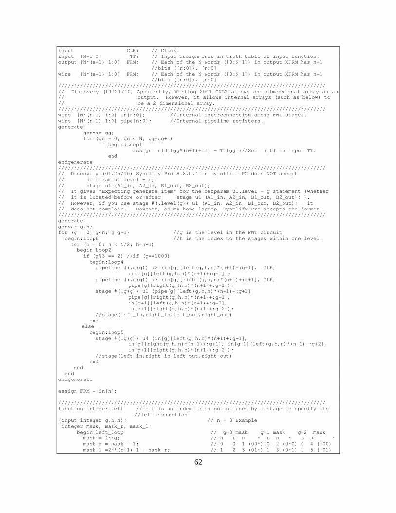
62
input CLK; // Clock. input [N-1:0] TT; // Input assignments in truth table of input function. output [N*(n+1)-1:0] FRM; // Each of the N words ([0:N-1]) in output XFRM has n+1 //bits ([n:0]). [n:0] wire [N*(n+1)-1:0] FRM; // Each of the N words ([0:N-1]) in output XFRM has n+1 //bits ([n:0]). [n:0] ////////////////////////////////////////////////////////////////////////////////////// // Discovery (01/21/10) Apparently, Verilog 2001 ONLY allows one dimensional array as an // output. However, it allows internal arrays (such as below) to // be a 2 dimensional array. ////////////////////////////////////////////////////////////////////////////////////// wire [N*(n+1)-1:0] in[n:0]; //Internal interconnection among FWT stages. wire [N*(n+1)-1:0] pipe[n:0]; //Internal pipeline registers. generate genvar gg; for (gg = 0; gg < N; gg=gg+1) begin:Loop1 assign in[0][gg*(n+1)+:1] = TT[gg];//Set in[0] to input TT. end endgenerate ////////////////////////////////////////////////////////////////////////////////////// // Discovery (01/25/10) Synplify Pro 8.8.0.4 on my office PC does NOT accept // defparam u1.level = g; // stage u1 (A1_in, A2_in, B1_out, B2_out); // It gives "Expecting generate item" for the defparam u1.level = g statement (whether // it is located before or after stage u1 (A1_in, A2_in, B1_out, B2_out); ). // However, if you use stage #(.level(g)) u1 (A1_in, A2_in, B1_out, B2_out); , it // does not complain. However, on my home laptop, Synplify Pro accepts the former. ////////////////////////////////////////////////////////////////////////////////////// generate genvar g,h; for (g = 0; g<n; g=g+1) //g is the level in the FWT circuit begin:Loop6 //h is the index to the stages within one level. for (h = 0; h < N/2; h=h+1) begin:Loop2 if (g%3 == 2) //if (g==1000) begin:Loop4 pipeline #(.g(g)) u2 (in[g][left(g,h,n)*(n+1)+:g+1], CLK, pipe[g][left(g,h,n)*(n+1)+:g+1]); pipeline #(.g(g)) u3 (in[g][right(g,h,n)*(n+1)+:g+1], CLK, pipe[g][right(g,h,n)*(n+1)+:g+1]); stage #(.g(g)) u1 (pipe[g][left(g,h,n)*(n+1)+:g+1], pipe[g][right(g,h,n)*(n+1)+:g+1], in[g+1][left(g,h,n)*(n+1)+:g+2], in[g+1][right(g,h,n)*(n+1)+:g+2]); //stage(left_in,right_in,left_out,right_out) end else begin:Loop5 stage #(.g(g)) u4 (in[g][left(g,h,n)*(n+1)+:g+1], in[g][right(g,h,n)*(n+1)+:g+1], in[g+1][left(g,h,n)*(n+1)+:g+2], in[g+1][right(g,h,n)*(n+1)+:g+2]); //stage(left_in,right_in,left_out,right_out) end end end endgenerate assign FRM = in[n]; ////////////////////////////////////////////////////////////////////////////////////// function integer left //left is an index to an output used by a stage to specify its //left connection. (input integer g,h,n); // n = 3 Example integer mask, mask_r, mask_l; begin:left_loop // g=0 mask g=1 mask g=2 mask mask = 2**g; // h L R * L R * L R * mask_r = mask - 1; // 0 0 1 (00*) 0 2 (0*0) 0 4 (*00) mask_l =2**(n-1)-1 - mask_r; // 1 2 3 (01*) 1 3 (0*1) 1 5 (*01)

63
left = ((mask_l & h)<<1) + (mask_r & h); // 2 4 5 (10*) 4 6 (1*0) 2 6 (*10) end // 3 6 7 (11*) 5 7 (1*1) 3 7 (*11) endfunction // // So, for g = 1, for example, we have function integer right //right is an index to an output used by a stage to specify its right connection. //mask = 2**g = 010, (input integer g,h,n); //mask_r = mask - 1 = 2 - 1 = 001, and integer mask, mask_r, mask_l; //mask_l = 2**(n-1)-1 - mask_r = 4-1 - 1 = 2 = 010 begin:right_loop // mask_l & mask_r extract from h, its l & r side. mask = 2**g; // left = (010&h)<<1 + 001&h. mask_r = mask - 1; // right = (010&h)<<1 + 010 + 001&h. mask_l = 2**(n-1)-1 - mask_r; // <<1 is to move mask_l left once to admit the * //bit. right = ((mask_l & h)<<1)+ (mask_r & h) + mask; end endfunction endmodule ////// RESULTS W/ NO PIPELINE REGISTERS Updated: 09/05/10 ////// //n = 1 2 3 4 5 6 7 8 9 10 //Freq. (MHz) 148.6 115.0 93.6 70.9 60.4 50.8 44.8 39.6 35.3 32.8 //#LUTs (%) 4(0%) 23(0%) 101(0%) 316(0%)797(1%) 2226(3%) 5700(8%) 14270(21%) 35548(52%) //85280(126%) // #Reg Bits 0 0 0 0 0 0 0 0 0 0 /////////////////////////////////////////////////////////////////////////////////////// ////// RESULTS W/ PIPELINE REGISTERS (g%3 == 1) Updated: 09/05/10 ////// //n = 1 2 3 4 5 6 7 8 9 10 //Freq. (MHz) 148.6 115.0 119.7 90.6 70.5 101.0 85.6 68.0 96.6 83.7 //#LUTs (%) 4(0%) 23(0%) 86(0%) 318(0%) 853(1%) 2278(3%) 5883(8%) 14772(21%) 36734(54%) //88443(130%) // #Reg Bits 0 0 0 0 0 0 0 0 0 0 /////////////////////////////////////////////////////////////////////////////////////// ////////////////////////////////////////////////////////////////////////////////////// ////////////////////////////////////////////////////////////////////////////////////// module stage(left_in, right_in, left_out, right_out); //--------------------------------------------------------------------------------------- // One stage only. Note that the structure of stage is independent of n, the number // of variables. It is dependent only on the level at which the stage resides. // parameter g = 3; /////////////////////////////// module inputs/outputs //////////////////////////////// // input [g:0] left_in; // left input. input [g:0] right_in; // left input. // output [g+1:0] left_out; // left output. output [g+1:0] right_out; // left output. reg [g+1:0] left_out; // left output. reg [g+1:0] right_out; // left output. reg [g+1:0] temp_right; reg [g+1:0] temp_left; // /////////////////////////////// module function //////////////////////////////// always @(*) begin // //Sign extend left_in and right_in unless = 100...0, in which case make it 0100...0. // This is done to accommodate 2^g >= Walsh coef >= -2^(g-1) (g+1 bits), as discussed // above. That is, the special case, Walsh coef = 2^g, is viewed as a positive integer. // instead of the usual negative integer. // if (left_in != 2**g)//{1'b1,{g{1'b0}}}) temp_left = {left_in[g],left_in}; else

64
temp_left = {1'b0,left_in}; // if (right_in != 2**g)//{1'b1,{g{1'b0}}}) temp_right = {right_in[g],right_in}; else temp_right = {1'b0,right_in}; // left_out = temp_left + temp_right; right_out = temp_left - temp_right; // end // endmodule ////////////////////////////////////////////////////////////////////////////////////// ////////////////////////////////////////////////////////////////////////////////////// ////////////////////////////////////////////////////////////////////////////////////// module pipeline(pipe_in, CLK, pipe_out); //--------------------------------------------------------------------------------------- // One stage only. Note that the structure of stage is independent of n, the number // of variables. It is dependent only on the level at which the stage resides. // parameter g = 64; /////////////////////////////// module inputs/outputs //////////////////////////////// input [g:0] pipe_in; input CLK; output [g:0] pipe_out; reg [g:0] pipe_out; //assign pipe_out = CLK?pipe_in:pipe_out; /This works also. always @(posedge CLK) pipe_out <= pipe_in; endmodule ////////////////////////////////////////////////////////////////////////////////////// module convert(CLK, coef_in, coef_out); //--------------------------------------------------------------------------------------- // This module takes the FWT coefficients and converts them to distances to linear // functions. // Specifically, this is already done for the first coefficients. A conversion is // needed for all of the other coefficients. // // The example below shows the conversion needed. // // c0 c1-c15 Add 8 If a>8 // a <- 16-a // // 10000 16 01000 8 10000 16 00000 0 // 01111 15 00111 7 01111 15 00001 1 // . // . // . // . // 00010 2 11010 -6 00010 2 00010 2 // 00001 1 11001 -7 00001 1 00001 1 // 00000 0 11000 -8 00000 0 00000 0 // // Author: Tim O'Dowd // Last Updated: 9/7/2010 parameter n = 3; // NUMBER OF VARIABLES IN FUNCTION

65
localparam N = 2**n; // NUMBER OF VALUES IN TRUTH TABLE OF FUNCTION localparam nn = n+1; // NUMBER OF BITS IN EACH WORD input [N*(n+1)-1:0] coef_in; // THIS IS THE FUNCTION'S FWT. IT HAS N WORDS EACH WITH n+1 BITS. FOR CASE // n = 4, THERE WILL BE 16 WORDS. EACH WORD WILL BE 5 BITS IN LENGTH. // TOTAL OF 16*5-1 = 80 BITS. HERE N*(n+1)-1 = 79. input CLK; // Clock input output [N*(n+1)-1:0] coef_out; //OUTPUT SHOULD BE SAME LENGTH AS INPUT reg [N*(n+1)-1:0] coef_out; reg [n:0] FWT; //variable to hold the parsed inputs corresponding to the FWT coefficients (see column //marked c1-c15 above) reg [n:0] a; //variable to hold modified FWT inputs (see column marked Add 8 above) integer g; //variable to increment FOR loop always@(posedge CLK) begin // the least significant input requires special handling FWT = coef_in [n:0]; a = FWT; if(a > N/2) a = N - a; coef_out[n:0] = a; // all other bits are handled here for (g = 1; g < N; g = g+1) // begin loop to go through input word by word starting with next to least significant nn bits begin:Loop1 FWT = coef_in [((g+1)*n+g)-:nn]; // Get the next most significant n bits of coef_in a = FWT + N/2; // Add N/2 to FWT to get value of a (EXCLUDING CASE OF LEAST SIGNIFICANT BIT) if (a > N/2) a = N - a; // If a is greater than N/2, then set a to N-a coef_out [((g+1)*n+g)-:nn] = a; // Store a in the appropriate bits in the output end // repeat loop end endmodule ////////////////////////////////////////////////////////////////////////////////////// module min(IN, OUT, CLK); //--------------------------------------------------------------------------------------- // min.v - A program to compare 2^(n+1) n+1-bit binary values and to deliver the // smallest to the output. This can be configured in two ways: // 1. Completely pipelined tree // 2. Completely combinational tree (except for a register at the output) // // In the case of 1. this runs a 209.6 MHz. for all values of n. It was // tr iedfor n up to 8. At n=8, it takes more than two minutes to compile. // // In the case of 2. the Freq. value is as follows // // n Freq. (MHz.) Total Runtime // 2 111.9 // 3 106.1 // 4 73.6 // 5 70.4 // 6 61.2 // 7 53.2 2 min. 45 secs. // 8 46.7 7 min. 57 secs.

66
// // To have a 1. Completely pipelined tree, use <= in three places // 1. curr_IN[0] <= IN; // ....................................................... // 2. if(curr_IN[j-1][((2*i + 2)*nn-1)-:nn] < // curr_IN[j-1][((2*i + 1)*nn-1)-:nn]) // curr_IN[j][((i + 1)*nn-1)-:nn] <= // curr_IN[j-1][((2*i + 2)*nn-1)-:nn]; // ....................................................... // 3. else curr_IN[j][((i + 1)*nn-1)-:nn] <= // curr_IN[j-1][((2*i + 1)*nn-1)-:nn]; // ....................................... // To have a 2. Completely combinational tree, use <= in three places // 1. curr_IN[0] = IN; // ....................................................... // 2. if(curr_IN[j-1][((2*i + 2)*nn-1)-:nn] < // curr_IN[j-1][((2*i + 1)*nn-1)-:nn]) // curr_IN[j][((i + 1)*nn-1)-:nn] = // curr_IN[j-1][((2*i + 2)*nn-1)-:nn]; // ....................................................... // 3. else curr_IN[j][((i + 1)*nn-1)-:nn] = // curr_IN[j-1][((2*i + 1)*nn-1)-:nn]; // ....................................................... // // NOTE: This produces many warnings that you have unused elements of a // matrix. // // // Created: November 7, 2007 // Last Modified: September 7, 2010 by Timothy O'Dowd // Author: Jon T. Butler // // Inputs: IN // Outputs: OUT // //--------------------------------------------------------------------------------------- // // NOTE: This program is the second time, I have used matrices. For example, curr_min // is the current minimum value. Using matrices provides control on the structure // of the circuit produced. parameter n = 4; // Number of variables. localparam nn = n + 1; // Number of bits in the numbers to be compared. localparam N = 2**n; // Number of numbers to be compared. (2**nn = 2^n) output [n:0] OUT; // OUT is the smallest of the n+1-bit inputs input [nn*N-1:0] IN; // IN is an array of 2^(n+1) (n+1)-bit numbers reg [nn*N-1:0] curr_IN [N:0]; input CLK; reg [n:0] curr_min [N:0]; integer i; always @(posedge CLK) begin curr_min[0] = {nn{1'b1}}; curr_IN[0] = IN; for(i=0; i<N; i=i+1) begin: increment curr_IN[i+1] <= curr_IN[i]; //Pipeline curr_IN if(curr_IN[i][((i+1)*nn-1)-:nn] < curr_min[i]) curr_min[i+1] <= curr_IN[i][((i+1)*nn-1)-:nn]; else curr_min[i+1] <= curr_min[i]; end end assign OUT = curr_min[N] ; endmodule //////////////////////////////////////////////////////////////////////////////////////
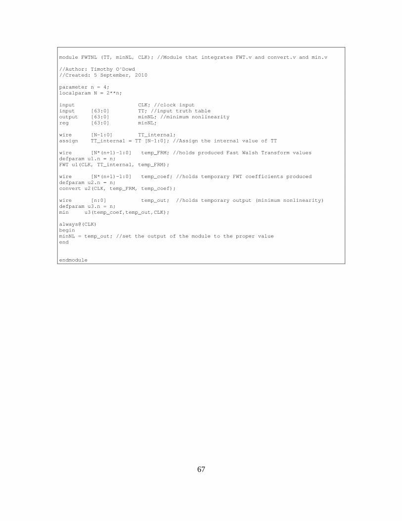
67
module FWTNL (TT, minNL, CLK); //Module that integrates FWT.v and convert.v and min.v //Author: Timothy O'Dowd //Created: 5 September, 2010 parameter n = 4; localparam N = 2**n; input CLK; //clock input input [63:0] TT; //input truth table output [63:0] minNL; //minimum nonlinearity reg [63:0] minNL; wire [N-1:0] TT_internal; assign TT_internal = TT [N-1:0]; //Assign the internal value of TT wire [N*(n+1)-1:0] temp_FRM; //holds produced Fast Walsh Transform values defparam u1.n = n; FWT u1(CLK, TT_internal, temp_FRM); wire [N*(n+1)-1:0] temp_coef; //holds temporary FWT coefficients produced defparam u2.n = n; convert u2(CLK, temp_FRM, temp_coef); wire [n:0] temp_out; //holds temporary output (minimum nonlinearity) defparam u3.n = n; min u3(temp_coef,temp_out,CLK); always@(CLK) begin minNL = temp_out; //set the output of the module to the proper value end endmodule

68
THIS PAGE INTENTIONALLY LEFT BLANK

69
APPENDIX B. MATLAB CODE
B1. ALGORITHM FOR PRODUCING BENT FUNCTION TRUTH TABLE
The code for the algorithm described in this thesis that is used to discover a
bent function's truth table given a nearby function's truth table is listed in this appendix.
This code is written for the case where n = 4, but can be modified in order to be used for
other n.
There are several files that are necessary for this algorithm to work properly.
FWT.m is a required file used to compute the FWT of a given TT. NL.m is a required file
used to compute the nonlinearity of a given FWT. functGen.m is a file that generates the
TT of all functions for a given n. FWT.m and NL.m are called by the other files.
functGen.m is called by files that seek to run the algorithm for sets of input functions.
NLfive.m, NLfour.m, and NLthree.m are files that find a function with
incrementally higher nonlinearity. They each require an input TT with a nonlinearity of
five, four, and three, respectively.
findbent3.m uses functGen.m to apply NLthree.m to every function with a
nonlinearity of three and produces functions with nonlinearity of four. findbent3to5.m is
similar, but takes all the functions that were produced with a nonlinearity of four and
inputs them to NLfour.m to produce output functions with nonlinearities of five.
findbent3to6.m takes this one step further, taking all functions produced with a
nonlinearity of five and applying NLfive.m to produce bent functions. All of these codes
count the number of successes, failures, and the unique functions produced.
findbent4.m and findbent5.m are analogous to findbent3.m. In addition,
findbent4to6.m is analogous to findbent3to6.m.

70
1. FWT.m
%% %Timothy O'Dowd %MATLAB Code to compute the Fast Walsh Transform of an input Truth Table %Written: Aug 1, 2010 %Modified: Nov 4, 2010 %INPUTS: %TT - the truth table of a Boolean function. TT MUST have length 2^n %n - the number of variables in the Boolean function. %OUTPUT: %FWT - the fast Walsh transform of the input TT %This code is written and verified for the n=4 case. It can be modified to work %for other values of n. Bent functions only exist for even n. function transform = FWT(TT,n) g = 0; %initialize g, which keeps track of iterations of butterfly modules h = 0; %initialize h, which keep track of how many pairs of butterflys have been computed curr = []; %array to keep track of current array next = []; %array to keep track of computed array delta = 2^g; %number to keep track of gap between left and right inputs into butterfly left = 1; right = left+delta; numPairs = 2^n/2;%number of butterfly pairs %paired = TT*0; %initliaze paired to an array the size of TT with all zero elements curr = TT; %set TT to current array for g=0:1:n-1 for h=1:1:numPairs delta = 2^g; %every further array has pairs spread further apart if g == 0 left = 2*h-1; right = left + delta; [next(left),next(right)] = butterfly(curr(left),curr(right)); elseif g == n-1

71
left = h; right = left + delta; [next(left),next(right)] = butterfly(curr(left),curr(right)); elseif h <= 2*g left = h; right = left + delta; [next(left),next(right)] = butterfly(curr(left),curr(right)); elseif h <= 4*g left = h + 2*g; right = left + delta; [next(left),next(right)] = butterfly(curr(left),curr(right)); elseif h <= 6*g left = h + 4*g; right = left + delta; [next(left),next(right)] = butterfly(curr(left),curr(right)); elseif h <= 8*g left = h + 6*g; right = left + delta; [next(left),next(right)] = butterfly(curr(left),curr(right)); end end curr = next; end transform = next; %return the FWT function [x,y] = butterfly(a,b) x = a+b; y = a-b; end end

72
2. NL.m
%% %Timothy O'Dowd %MATLAB Code to compute the Nonlinearity of an input FWT %Written: Aug 1, 2010 %Modified: Nov 4, 2010 %INPUTS: %FWT - the Fast Walsh Transform of a Boolean function. FWT MUST have length 2^n %n - the number of variables in the Boolean function. %OUTPUT: %nonlinearity - the nonlinearity of a Boolean function %this code works for any value of n function nonlinearity = NL(FWT,n) a = FWT; %put FWT into working array for i=2:1:2^n a(i) = a(i) + 2^n/2; %normalize a end for i=1:1:2^n if a(i) >= 2^n/2 a(i) = 2^n - a(i); %take absolute value of a end end nonlinearity = min(a); %return nonlinearity end

73
3. functGen.m
%% %Timothy O'Dowd %MATLAB Code to compute the Nonlinearity of an input FWT %Written: Aug 1, 2010 %Modified: Nov 4, 2010 %INPUTS: %n - the number of variables in the Boolean function. %init - variable indicating the first call to the function % 0 = first call; any other value valid for subsequent calls %current - last function generated % for first call any value is valid %OUTPUT: %exec - next TT sequentially %this code works for any value of n function exec = functGen(n,init,current) initial = []; %initialize initial for q=1:1:2^n initial = [initial 0]; %create properly sized array full of zeros end if init == 0 %denotes the first call of this function current = initial; end %for f = 1:1:10 %2^(2^n) %repeat 2^(2^n) times if init ~= 0 t = 1; %set t to 1 good = 1; while (good) %t = 1:1:2^n %for every bit of TT if (current(t) == 1) %if current bit being looked at is already a one current(t) = 0; %set it to zero t = t + 1; %and look at next bit else current(t) = 1; %if not, set bit to 1 and end good = 0; %terminate loop end end end %end exec = current; end

74
4. NLthree.m
%% %Timothy O'Dowd %MATLAB Code to implement algorithm to search for a function with NL=4 % given a function with NL=3 %Written: Sep 12, 2010 %Modified: Nov 15, 2010 %INPUTS: %TT - the truth table of a Boolean function. TT MUST have length 2^n %n - the number of variables in the Boolean function. %OUTPUT: %truth - the truth table of a function nonlinearity increased by one %nonlin - the nonlinearity of the output function %This code is written and verified for the n=4 case. It can be modified %to work for other values of n. Bent functions only exist for even n. function [truth,nonlin] = NLthree(TT,n) bentNL = 2^(n-1)-2^(n/2-1); %any bent function will have this NL bentweightLow = 2^(n-1)-2^(n/2-1); %low value of a bent function's %weight bentweightHigh = 2^(n-1)+2^(n/2-1); %high value of a bent function's %weight nextTT = TT; %iterative TT array nextFWT = FWT(TT,n); %iterative FWT array oldTT = TT; %storage for previous TT oldFWT = nextFWT; %storage for previous FWT nextnonlin = NL(nextFWT,n); %iterative value of nonlin t = 0; %t is TT index search variable f = 2; %FWT index search variable variable good = 1; %variable used to turn on/off while loop switchedbit = 0; %variable used to indicate if bit has been %complemented fail = 0; %indicates algorithm failure %matrix that holds information about how FWT changes as input TT is %changed TTvsFWT4 = [1 1 1 1 1 1 1 1 1 1 1 1 1 1 1 1; 1 -1 1 -1 1 -1 1 -1 1 -1 1 -1 1 -1 1 -1; 1 1 -1 -1 1 1 -1 -1 1 1 -1 -1 1 1 -1 -1; 1 -1 -1 1 1 -1 -1 1 1 -1 -1 1 1 -1 -1 1; 1 1 1 1 -1 -1 -1 -1 1 1 1 1 -1 -1 -1 -1; 1 -1 1 -1 -1 1 -1 1 1 -1 1 -1 -1 1 -1 1; 1 1 -1 -1 -1 -1 1 1 1 1 -1 -1 -1 -1 1 1; 1 -1 -1 1 -1 1 1 -1 1 -1 -1 1 -1 1 1 -1; 1 1 1 1 1 1 1 1 -1 -1 -1 -1 -1 -1 -1 -1;

75
1 -1 1 -1 1 -1 1 -1 -1 1 -1 1 -1 1 -1 1; 1 1 -1 -1 1 1 -1 -1 -1 -1 1 1 -1 -1 1 1; 1 -1 -1 1 1 -1 -1 1 -1 1 1 -1 -1 1 1 -1; 1 1 1 1 -1 -1 -1 -1 -1 -1 -1 -1 1 1 1 1; 1 -1 1 -1 -1 1 -1 1 -1 1 -1 1 1 -1 1 -1; 1 1 -1 -1 -1 -1 1 1 -1 -1 1 1 1 1 -1 -1; 1 -1 -1 1 -1 1 1 -1 -1 1 1 -1 1 -1 -1 1]; disp('Input Truth Table is:') disp(TT) disp('Fast Walsh Transform is:') disp(nextFWT) disp('Nonlinearity is:') disp(nextnonlin) while (nextnonlin < bentNL-2 && ~fail) %if function has NL = 3 and fail condition isn't set, use algorithm %In this case, the TT needs three 0's to become 1's if (nextFWT(1) == bentweightLow-3) %find the next 0 in the TT to change and increment TT counter t = t + 1; %increment t if t > 2^n %here, there is no 0->1 transition that works fail = 1; %set fail condition! t = 1; %reset t to one end while (nextTT(t)== 1 && ~fail) t = t + 1; if t > 2^n %here, there is no 0->1 transition that works fail = 1; %set fail condition! t = 1; %reset t to one end f = 2; %reset f when a new value of TT entry is used end if(~fail) for f=2:1:2^n %test each element of FWT to see if changing t %in TT would give function with LOWER nonlinearity if TTvsFWT4(t,f) == -1 && nextFWT(f) == -5 || TTvsFWT4(t,f) == 1 && nextFWT(f) == 5 good = 0; %if potential transition gives LOWER %nonlinearity we do not try this transistion end end if (good) %if criteria is met, we try the transition disp('Complementing bit:') t oldTT = nextTT; %store old TT

76
nextTT(t) = nextTT(t)+1; %make 0->1 transition in the TT oldFWT = nextFWT; %store old FWT nextFWT = FWT(nextTT,n); %get FWT of new TT nextnonlin = NL(nextFWT,n); %check to see if transition %increased nonlinearity switchedbit = 1; end %this portion of code should never be used. a transition will %never be made due to the checks performed above if (nextnonlin < bentNL-2 && switchedbit) %check to see if %transition worked disp('Unsuccessful bit chosen. Restoring original Truth Table') nextTT = oldTT; %if not, undo transition t = t + 1; %try again with next digit nextFWT = oldFWT; %and restore old FWT switchedbit = 0; %reset end good = 1; %reset good end end %In this case, the TT needs three 1s to become 0s if nextFWT(1) == bentweightHigh+3 %find the next 0 in the TT to change and increment TT counter t = t + 1; %increment t if t > 2^n %here, there is no 0->1 transition that works fail = 1; %set fail condition t = 1; %reset t to one end while (nextTT(t)== 0 && ~fail) t = t + 1; if t > 2^n %here, there is no 0->1 transition that works fail = 1; %set fail condition t = 1; %reset t to one end f = 2; %reset f when a new value of TT entry is used end if(~fail) for f=2:1:2^n %test each element of FWT to see if changing %t in TT would give LOWER nonlinearity if TTvsFWT4(t,f) == -1 && nextFWT(f) == 5 || TTvsFWT4(t,f) == 1 && nextFWT(f) == -5 good = 0; %if criteria is met we will move on to %next possible transition end end

77
if (good) %if criteria is met, we try the transition disp('Complementing bit:') t oldTT = nextTT; %store old TT nextTT(t) = nextTT(t)-1; %make 1->0 transition in the TT oldFWT = nextFWT; %store old FWT nextFWT = FWT(nextTT,n); %get FWT of new TT nextnonlin = NL(nextFWT,n); %check to see if transition %increased nonlinearity switchedbit = 1; end %this portion of code should never be used. a transition will %never be made due to the checks performed above if (nextnonlin < bentNL-2 && switchedbit) %check to see if %transition worked disp('Unsuccessful bit chosen. Restoring original Truth Table') nextTT = oldTT; %if not, undo transition t = t + 1; %try again with next digit nextFWT = oldFWT; %and restore old FWT switchedbit = 0; %reset end good = 1; %reset good end end %In this case, the TT correct number of 1's/0's (ambiguous %case) This program DEFAULTS to ADDING a 1 if nextFWT(1) == bentweightLow - 1 || nextFWT(1) == bentweightLow + 1 || nextFWT(1) == bentweightHigh -1 || nextFWT(1) == bentweightHigh + 1 %find the next 0 in the TT to change and increment TT counter t = t + 1; %increment t if t > 2^n %here, there is no 0->1 transition that works fail = 1; %note that 1->0 transition is needed t = 1; %reset t to one end while (nextTT(t)== 1 && ~fail) t = t + 1; if t > 2^n %here, there is no 0->1 transition that works fail = 1; %note that 1->0 transition is needed t = 1; %reset t to one end f = 2; %reset f when a new value of TT entry is used end if(~fail) for f=2:1:2^n %test each element of FWT to see if changing %t in TT would give LOWER nonlinearity

78
if TTvsFWT4(t,f) == 1 && nextFWT(f) == 5 || TTvsFWT4(t,f) == -1 && nextFWT(f) == -5 good = 0; %if criteria is not met we will move on %to next possible transition end end if (good) %if criteria is met, we try the transition disp('Complementing bit:') t oldTT = nextTT; %store old TT nextTT(t) = nextTT(t)+1; %make 1->0 transition in the TT oldFWT = nextFWT; %store old FWT nextFWT = FWT(nextTT,n); %get FWT of new TT nextnonlin = NL(nextFWT,n); %check to see if transition %increased nonlinearity switchedbit = 1; end %this portion of code should never be used. a transition will %never be made due to the checks performed above if (nextnonlin < bentNL-2 && switchedbit) %check to see if %transition worked disp('Unsuccessful bit chosen. Restoring original Truth Table') nextTT = oldTT; %if not, undo transition t = t + 1; %try again with next digit nextFWT = oldFWT; %and restore old FWT switchedbit = 0; %reset end good = 1; %reset good end end end if(~fail) truth = nextTT; nonlin = nextnonlin; disp('Correct bit chosen!') disp('') disp('New Truth Table:') disp(truth) disp('Nonlinearity is:') disp(nextnonlin) else disp('Algorithm Failure')

79
truth = [0 0 0 0 0 0 0 0 0 0 0 0 0 0 0 0]; %output array that signals failure nonlin = 500; %indicates a failure end end
5. NLfour.m
%% %Timothy O'Dowd %MATLAB Code to implement algorithm to search for a function with NL=4 % given a function with NL=3 %Written: Sep 12, 2010 %Modified: Nov 15, 2010 %INPUTS: %TT - the truth table of a Boolean function. TT MUST have length 2^n %n - the number of variables in the Boolean function. %OUTPUT: %truth - the truth table of a function nonlinearity increased by one %nonlin - the nonlinearity of the output function %This code is written and verified for the n=4 case. It can be modified %to work for other values of n. Bent functions only exist for even n. function [truth,nonlin] = NLthree(TT,n) bentNL = 2^(n-1)-2^(n/2-1); %any bent function will have this NL bentweightLow = 2^(n-1)-2^(n/2-1); %low value of a bent function's %weight bentweightHigh = 2^(n-1)+2^(n/2-1); %high value of a bent function's %weight nextTT = TT; %iterative TT array nextFWT = FWT(TT,n); %iterative FWT array oldTT = TT; %storage for previous TT oldFWT = nextFWT; %storage for previous FWT nextnonlin = NL(nextFWT,n); %iterative value of nonlin t = 0; %t is TT index search variable f = 2; %FWT index search variable variable good = 1; %variable used to turn on/off while loop switchedbit = 0; %variable used to indicate if bit has been %complemented fail = 0; %indicates algorithm failure %matrix that holds information about how FWT changes as input TT is %changed TTvsFWT4 = [1 1 1 1 1 1 1 1 1 1 1 1 1 1 1 1; 1 -1 1 -1 1 -1 1 -1 1 -1 1 -1 1 -1 1 -1;

80
1 1 -1 -1 1 1 -1 -1 1 1 -1 -1 1 1 -1 -1; 1 -1 -1 1 1 -1 -1 1 1 -1 -1 1 1 -1 -1 1; 1 1 1 1 -1 -1 -1 -1 1 1 1 1 -1 -1 -1 -1; 1 -1 1 -1 -1 1 -1 1 1 -1 1 -1 -1 1 -1 1; 1 1 -1 -1 -1 -1 1 1 1 1 -1 -1 -1 -1 1 1; 1 -1 -1 1 -1 1 1 -1 1 -1 -1 1 -1 1 1 -1; 1 1 1 1 1 1 1 1 -1 -1 -1 -1 -1 -1 -1 -1; 1 -1 1 -1 1 -1 1 -1 -1 1 -1 1 -1 1 -1 1; 1 1 -1 -1 1 1 -1 -1 -1 -1 1 1 -1 -1 1 1; 1 -1 -1 1 1 -1 -1 1 -1 1 1 -1 -1 1 1 -1; 1 1 1 1 -1 -1 -1 -1 -1 -1 -1 -1 1 1 1 1; 1 -1 1 -1 -1 1 -1 1 -1 1 -1 1 1 -1 1 -1; 1 1 -1 -1 -1 -1 1 1 -1 -1 1 1 1 1 -1 -1; 1 -1 -1 1 -1 1 1 -1 -1 1 1 -1 1 -1 -1 1]; disp('Input Truth Table is:') disp(TT) disp('Fast Walsh Transform is:') disp(nextFWT) disp('Nonlinearity is:') disp(nextnonlin) %Only run if input function has NL = 4 and fail condition not met while (nextnonlin < bentNL-2 && ~fail) %In this case, the TT needs three 0's to become 1's if (nextFWT(1) == bentweightLow-3) %find the next 0 in the TT to change and increment TT %counter t = t + 1; %increment t if t > 2^n %here, there is no 0->1 transition that works fail = 1; %set fail! t = 1; %reset t to one end while (nextTT(t)== 1 && ~fail) t = t + 1; if t > 2^n %here, there is no 0->1 transition that %works fail = 1; %set fail! t = 1; %reset t to one end f = 2; %reset f when a new value of TT entry is used end if(~fail) for f=2:1:2^n %test each element of FWT to see if changing %in TT would give function with LOWER nonlinearity if TTvsFWT4(t,f) == -1 && nextFWT(f) == -5 || TTvsFWT4(t,f) == 1 && nextFWT(f) == 5

81
good = 0; %if potential transition gives LOWER %nonlinearity we do not try this transistion end end if (good) %if criteria is met, we try the transition disp('Complementing bit:') t oldTT = nextTT; %store old TT nextTT(t) = nextTT(t)+1; %make 0->1 transition in the TT oldFWT = nextFWT; %store old FWT nextFWT = FWT(nextTT,n); %get FWT of new TT nextnonlin = NL(nextFWT,n); %check to see if transition %increased nonlinearity switchedbit = 1; end %this portion of code should never be used. a transition will %never be made due to the checks performed above if (nextnonlin < bentNL-2 && switchedbit) %check to see if %transition worked disp('Unsuccessful bit chosen. Restoring original Truth Table') nextTT = oldTT; %if not, undo transition t = t + 1; %try again with next digit nextFWT = oldFWT; %and restore old FWT switchedbit = 0; %reset end good = 1; %reset good end end %In this case, the TT needs three 1s to become 0s if nextFWT(1) == bentweightHigh+3 %find the next 0 in the TT to change and increment TT counter t = t + 1; %increment t if t > 2^n %here, there is no 0->1 transition that works fail = 1; %set fail t = 1; %reset t to one end while (nextTT(t)== 0 && ~fail) t = t + 1; if t > 2^n %here, there is no 0->1 transition that %works fail = 1; %set fail t = 1; %reset t to one end f = 2; %reset f when a new value of TT entry is used end

82
if(~fail) for f=2:1:2^n %test each element of FWT to see if changing %t in TT would give LOWER nonlinearity if TTvsFWT4(t,f) == -1 && nextFWT(f) == 5 || TTvsFWT4(t,f) == 1 && nextFWT(f) == -5 good = 0; %if criteria is met we will move on to %next possible transition end end if (good) %if criteria is met, we try the transition disp('Complementing bit:') t oldTT = nextTT; %store old TT nextTT(t) = nextTT(t)-1; %make 1->0 transition in the TT oldFWT = nextFWT; %store old FWT nextFWT = FWT(nextTT,n); %get FWT of new TT nextnonlin = NL(nextFWT,n); %check to see if transition %increased nonlinearity switchedbit = 1; end %this portion of code should never be used. a transition will %never be made due to the checks performed above if (nextnonlin < bentNL-2 && switchedbit) %check to see if %transition worked disp('Unsuccessful bit chosen. Restoring original Truth Table') nextTT = oldTT; %if not, undo transition t = t + 1; %try again with next digit nextFWT = oldFWT; %and restore old FWT switchedbit = 0; %reset end good = 1; %reset good end end %In this case, the TT correct number of 1's/0's (ambiguous %case) This program DEFAULTS to ADDING a 1 if nextFWT(1) == bentweightLow - 1 || nextFWT(1) == bentweightLow + 1 || nextFWT(1) == bentweightHigh -1 || nextFWT(1) == bentweightHigh + 1 %find the next 0 in the TT to change and increment TT counter t = t + 1; %increment t if t > 2^n %here, there is no 0->1 transition that works fail = 1; %set fail t = 1; %reset t to one end while (nextTT(t)== 1 && ~fail) t = t + 1;

83
if t > 2^n %here, there is no 0->1 transition that %works fail = 1; %set fail t = 1; %reset t to one end f = 2; %reset f when a new value of TT entry is used end if(~fail) for f=2:1:2^n %test each element of FWT to see if changing %t in TT would give LOWER nonlinearity if TTvsFWT4(t,f) == 1 && nextFWT(f) == 5 || TTvsFWT4(t,f) == -1 && nextFWT(f) == -5 good = 0; %if criteria is not met we will move on %to next possible transition end end if (good) %if criteria is met, we try the transition disp('Complementing bit:') t oldTT = nextTT; %store old TT nextTT(t) = nextTT(t)+1; %make 1->0 transition in the TT oldFWT = nextFWT; %store old FWT nextFWT = FWT(nextTT,n); %get FWT of new TT nextnonlin = NL(nextFWT,n); %check to see if transition %increased nonlinearity switchedbit = 1; end %this portion of code should never be used. a transition will %never be made due to the checks performed above if (nextnonlin < bentNL-2 && switchedbit) %check to see if %transition worked disp('Unsuccessful bit chosen. Restoring original Truth Table') nextTT = oldTT; %if not, undo transition t = t + 1; %try again with next digit nextFWT = oldFWT; %and restore old FWT switchedbit = 0; %reset end good = 1; %reset good end end end

84
if(~fail) truth = nextTT; nonlin = nextnonlin; disp('Correct bit chosen!') disp('') disp('New Truth Table:') disp(truth) disp('Nonlinearity is:') disp(nextnonlin) else disp('Algorithm Failure') truth = [0 0 0 0 0 0 0 0 0 0 0 0 0 0 0 0]; %output array that %signals failure nonlin = 500; %indicates a failure end end
6. NLfive.m
%% %Timothy O'Dowd %MATLAB Code to implement algorithm to search for a bent function %Written: Sep 12, 2010 %Modified: Nov 15, 2010 %INPUTS: %TT - the truth table of a Boolean function. TT MUST have length 2^n %n - the number of variables in the Boolean function. %OUTPUT: %truth - the truth table of a bent function. %nonlin - the nonlinearity of the output functions %Note: This code is written and verified for the n=4 case. It can be modified to work %for other values of n. Bent functions only exist for even n. function [truth,nonlin] = NLfive(TT,n) bentNL = 2^(n-1)-2^(n/2-1); %any bent function will have this NL bentweightLow = 2^(n-1)-2^(n/2-1); %low value of a bent function's %weight bentweightHigh = 2^(n-1)+2^(n/2-1); %high value of a bent function's %weight nextTT = TT; %iterative TT array nextFWT = FWT(TT,n); %iterative FWT array oldTT = TT; %storage for previous TT oldFWT = nextFWT; %storage for previous FWT

85
nextnonlin = NL(TT,n); %iterative value of nonlin t = 0; %t is TT index search variable f = 2; %FWT index search variable variable good = 1; %variable used to turn on/off while loop switchedbit = 0; %variable used to indicate whether bit has been %complemented %matrix that holds information about how FWT changes as input TT is %changed TTvsFWT4 = [1 1 1 1 1 1 1 1 1 1 1 1 1 1 1 1; 1 -1 1 -1 1 -1 1 -1 1 -1 1 -1 1 -1 1 -1; 1 1 -1 -1 1 1 -1 -1 1 1 -1 -1 1 1 -1 -1; 1 -1 -1 1 1 -1 -1 1 1 -1 -1 1 1 -1 -1 1; 1 1 1 1 -1 -1 -1 -1 1 1 1 1 -1 -1 -1 -1; 1 -1 1 -1 -1 1 -1 1 1 -1 1 -1 -1 1 -1 1; 1 1 -1 -1 -1 -1 1 1 1 1 -1 -1 -1 -1 1 1; 1 -1 -1 1 -1 1 1 -1 1 -1 -1 1 -1 1 1 -1; 1 1 1 1 1 1 1 1 -1 -1 -1 -1 -1 -1 -1 -1; 1 -1 1 -1 1 -1 1 -1 -1 1 -1 1 -1 1 -1 1; 1 1 -1 -1 1 1 -1 -1 -1 -1 1 1 -1 -1 1 1; 1 -1 -1 1 1 -1 -1 1 -1 1 1 -1 -1 1 1 -1; 1 1 1 1 -1 -1 -1 -1 -1 -1 -1 -1 1 1 1 1; 1 -1 1 -1 -1 1 -1 1 -1 1 -1 1 1 -1 1 -1; 1 1 -1 -1 -1 -1 1 1 -1 -1 1 1 1 1 -1 -1; 1 -1 -1 1 -1 1 1 -1 -1 1 1 -1 1 -1 -1 1]; disp('Input Truth Table is:') disp(TT) disp('Fast Walsh Transform is:') disp(nextFWT) disp('Nonlinearity is:') disp(nextnonlin) while (nextnonlin < bentNL) %if function ISNT bent, use algorithm %In this case, the TT needs one 0 to become a 1 if (nextFWT(1) == bentweightLow-1 || nextFWT(1) == bentweightHigh-1) %find the next 0 in the TT to change and increment TT %counter t = t + 1; %increment t while (nextTT(t)== 1) t = t + 1; f = 2; %reset f when a new value of TT entry is used end for f=2:1:2^n %test each element of FWT to see if changing %t in TT would give bent function

86
if TTvsFWT4(t,f) == -1 && nextFWT(f) == 3 || TTvsFWT4(t,f) == -1 && nextFWT(f) == -1 || TTvsFWT4(t,f) == 1 && nextFWT(f) == 1 || TTvsFWT4(t,f) == 1 && nextFWT(f) == -3 else good = 0; %if criteria is not met we will move on %to next possible transition end end if (good) %if criteria is met, we try the transition disp('Complementing bit:') disp(t) oldTT = nextTT; %store old TT nextTT(t) = nextTT(t)+1 %make 0->1 transition in the TT oldFWT = nextFWT; %store old FWT nextFWT = FWT(nextTT,n); %get FWT of new TT nextnonlin = NL(nextFWT,n); %check to see if transition %increased nonlinearity switchedbit = 1; %used to indicate if transition was %made end %this portion of code should never be used. a transition will %never be made due to the checks performed above if (nextnonlin < bentNL && switchedbit) %check to see if %transition worked disp('Unsuccessful bit chosen. Restoring original Truth Table') disp(t) nextTT = oldTT; %if not, undo transition t = t + 1; %try again with next digit nextFWT = oldFWT; %and restore old FWT switchedbit = 0; %reset end good = 1; %reset good end %In this case, the TT needs one 1 to become a 0 if nextFWT(1) == bentweightLow+1 || nextFWT(1) == bentweightHigh+1 %find the next 1 in the TT to change and increment TT counter t = t + 1; %increment t while (nextTT(t)== 0) t = t + 1; f = 2; %reset f when a new value of TT entry is used end

87
for f=2:1:2^n %test each element of FWT to see if changing %t in TT would give bent function if TTvsFWT4(t,f) == 1 && nextFWT(f) == 3 || TTvsFWT4(t,f) == 1 && nextFWT(f) == -1|| TTvsFWT4(t,f) == -1 && nextFWT(f) == 1 || TTvsFWT4(t,f) == -1 && nextFWT(f) == -3 else good = 0; %if criteria is not met we will move on %to next possible transition end end if (good) %if criteria is met, we try the transition disp('Complementing bit:') disp(t) oldTT = nextTT; %store old TT nextTT(t) = nextTT(t)-1; %make 1->0 transition in the TT oldFWT = nextFWT; %store old FWT nextFWT = FWT(nextTT,n); %get FWT of new TT nextnonlin = NL(nextFWT,n); %check to see if transition %increased nonlinearity switchedbit = 1; %used to indicate if transition was %made end %this portion of code should never be used. a transition will %never be made due to the checks performed above if (nextnonlin < bentNL && switchedbit) %check to see if %transition worked disp('Unsuccessful bit chosen. Restoring original Truth Table') disp(t) nextTT = oldTT; %if not, undo transition t = t + 1; %try again with next digit nextFWT = oldFWT; %and restore old FWT switchedbit = 0; %reset end good = 1; %reset good end end disp('Correct bit chosen!') disp('') disp('Bent Function Truth Table:') truth = nextTT; nonlin = nextnonlin; end

88
7. findbent3.m
%% %Timothy O'Dowd %MATLAB Code to implement algorithm to for functions with NL=4 given %ALL functions with NL=3 %Written: Sep 12, 2010 %Modified: Nov 4, 2010 %INPUTS: %n - the number of variables in the Boolean function. %OUTPUTS: none % %This program will display the number of functions tested, the number %of successes, the number of failures, and the number of unique %functions produced by successes.. %This code is written for the n=4 case. It can be modified to work %for other values of n. Bent functions only exist for even n. function [] = findbent3(n) bentNL = 2^(n-1)-2^(n/2-1); %any bent function will have this NL bent = 0; %counts unique number of functions found numberTested = 0; %counts number of functions tested failures = 0; %counts number of algorithm failures success = 0; %counts number of algorithm successes bentTT = []; %gathers bent function TTs TT = functGen(n,0,0); %generate first function to be tested truth = []; %initialize truth array for t=1:1:2^(2^n) if(~isequal(TT,[1 1 1 1 1 1 1 1 1 1 1 1 1 1 1 1 ])) %stop if 1 %function is reached TT = functGen(n,t,TT)%get next TT end a = FWT(TT,n); %find the FWT of the input TT nonlin = NL(a,n); %find the NL of the input TT while (nonlin == bentNL-3) %Only examine for NL = 3 [truth,nonlin] = NLthree(TT,n); %produce TT with higher NL numberTested = numberTested + 1; if (nonlin == bentNL-2)

89
bentTT = [bentTT;truth]; %if function with NL=4 produced, %collect it success = success + 1; end if (isequal(truth,[0 0 0 0 0 0 0 0 0 0 0 0 0 0 0 0])) failures = failures + 1; %count a failure if algorithm returned %failure array end end end [bent sizeBent] = size(unique(bentTT,'rows')) %Bent returns the number %of UNIQUE functions with NL=4 found numberTested success failures end
8. findbent3to5.m
%% %Timothy O'Dowd %MATLAB Code to implement algorithm to search for a functions %with NL=5 given all functions with NL=3 %Written: Sep 12, 2010 %Modified: Nov 4, 2010 %INPUTS: %n - the number of variables in the Boolean function. %OUTPUTS: none % %This program will display the number of functions tested, the number %of successes, the number of failures, and the number of unique %functions produced by successes. %This code is written for the n=4 case. It can be modified to work %for other values of n. Bent functions only exist for even n. function [] = findbent3to5(n) bentNL = 2^(n-1)-2^(n/2-1); %any bent function will have this NL bent = 0; %counts unique number of functions found numberTested = 0; %counts number of functions tested
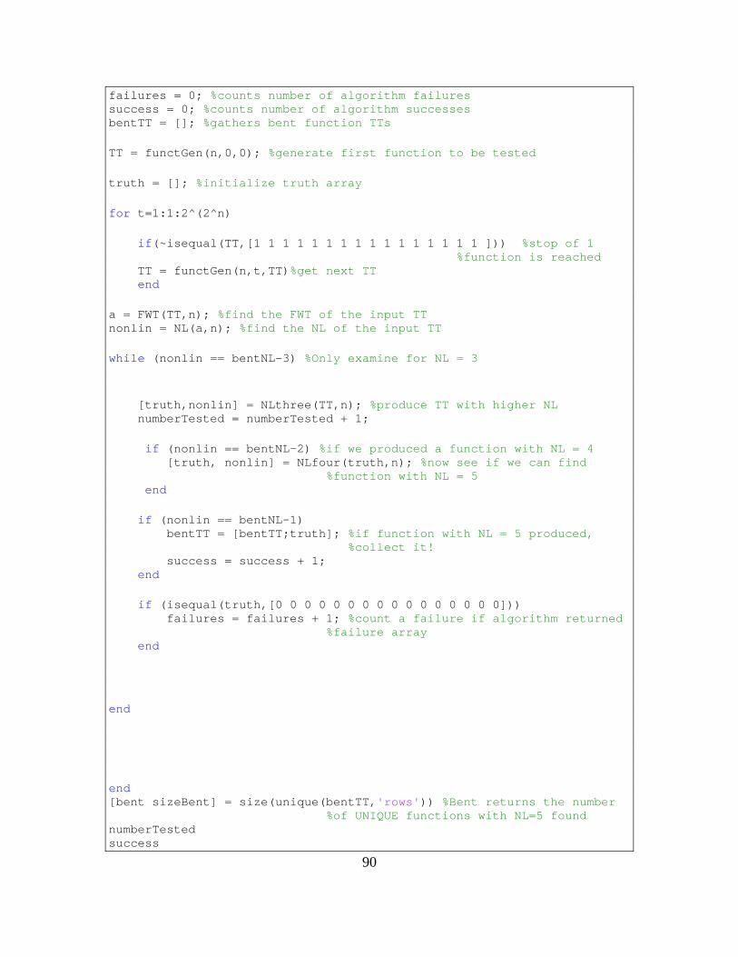
90
failures = 0; %counts number of algorithm failures success = 0; %counts number of algorithm successes bentTT = []; %gathers bent function TTs TT = functGen(n,0,0); %generate first function to be tested truth = []; %initialize truth array for t=1:1:2^(2^n) if(~isequal(TT,[1 1 1 1 1 1 1 1 1 1 1 1 1 1 1 1 ])) %stop of 1 %function is reached TT = functGen(n,t,TT)%get next TT end a = FWT(TT,n); %find the FWT of the input TT nonlin = NL(a,n); %find the NL of the input TT while (nonlin == bentNL-3) %Only examine for NL = 3 [truth,nonlin] = NLthree(TT,n); %produce TT with higher NL numberTested = numberTested + 1; if (nonlin == bentNL-2) %if we produced a function with NL = 4 [truth, nonlin] = NLfour(truth,n); %now see if we can find %function with NL = 5 end if (nonlin == bentNL-1) bentTT = [bentTT;truth]; %if function with NL = 5 produced, %collect it! success = success + 1; end if (isequal(truth,[0 0 0 0 0 0 0 0 0 0 0 0 0 0 0 0])) failures = failures + 1; %count a failure if algorithm returned %failure array end end end [bent sizeBent] = size(unique(bentTT,'rows')) %Bent returns the number %of UNIQUE functions with NL=5 found numberTested success

91
failures end
9. findbent3to6.m
%% %Timothy O'Dowd %MATLAB Code to implement algorithm to search for a bent function %given ALL functions with NL=3 as inputs %Written: Sep 12, 2010 %Modified: Nov 4, 2010 %INPUTS: %n - the number of variables in the Boolean function. %OUTPUTS: none % %This program will display the number of functions tested, the number %of successes, the number of failures, and the number of unique %functions produced by successes. %This code is written for the n=4 case. It can be modified to work %for other values of n. Bent functions only exist for even n. function [] = findbent3to6(n) bentNL = 2^(n-1)-2^(n/2-1); %any bent function will have this NL bent = 0; %counts unique number of functions found numberTested = 0; %counts number of functions tested failures = 0; %counts number of algorithm failures success = 0; %counts number of algorithm successes bentTT = []; %gathers bent function TTs TT = functGen(n,0,0); %generate first function to be tested truth = []; %initialize truth array for t=1:1:2^(2^n) if(~isequal(TT,[1 1 1 1 1 1 1 1 1 1 1 1 1 1 1 1 ])) %stop if 1 %function is reached TT = functGen(n,t,TT)%get next TT end a = FWT(TT,n); %find the FWT of the input TT nonlin = NL(a,n); %find the NL of the input TT while (nonlin == bentNL-3) %Only examine for NL = 3

92
[truth,nonlin] = NLthree(TT,n); %produce TT with higher NL numberTested = numberTested + 1; if (nonlin == bentNL-2) %if we produced a function with NL = 4 [truth, nonlin] = NLfour(truth,n); %now see if we can find %function with NL = 5 end if (nonlin == bentNL-1) [truth, nonlin] = NLfive(truth,n); %now see if we can find a %bent function! bentTT = [bentTT;truth]; %if bent function produced, collect it success = success + 1; end if (isequal(truth,[0 0 0 0 0 0 0 0 0 0 0 0 0 0 0 0])) failures = failures + 1; %count a failure if algorithm returned %failure array end end end [bent sizeBent] = size(unique(bentTT,'rows')) %Bent returns the number %of UNIQUE bent functions found numberTested success failures end
10. findbent4.m
%% %Timothy O'Dowd %MATLAB Code to implement algorithm to search for a functions %with NL=5 given ALL functions with NL=4 %Written: Sep 12, 2010 %Modified: Nov 4, 2010 %INPUTS: %n - the number of variables in the Boolean function. %OUTPUTS: none % %This program will display the number of functions tested, the number %of successes, the number of failures, and the number of unique %functions produced by successes. %This code is written for the n=4 case. It can be modified to work %for other values of n. Bent functions only exist for even n.

93
function [] = findbent4(n) bentNL = 2^(n-1)-2^(n/2-1); %any bent function will have this NL bent = 0; %counts unique number of functions found numberTested = 0; %counts number of functions tested failures = 0; %counts number of algorithm failures success = 0; %counts number of algorithm successes bentTT = []; %gathers bent function TTs TT = functGen(n,0,0); %generate first function to be tested truth = []; %initialize truth array for t=1:1:2^(2^n) if(~isequal(TT,[1 1 1 1 1 1 1 1 1 1 1 1 1 1 1 1 ])) %stop if 1 %function is reached TT = functGen(n,t,TT)%get next TT end a = FWT(TT,n); %find the FWT of the input TT nonlin = NL(a,n); %find the NL of the input TT while (nonlin == bentNL-2) %Only examine for NL = 4 [truth,nonlin] = NLfour(TT,n); %produce TT with higher NL numberTested = numberTested + 1; if (nonlin == bentNL-1) bentTT = [bentTT;truth]; %if bent function produced, collect it success = success + 1; end if (isequal(truth,[0 0 0 0 0 0 0 0 0 0 0 0 0 0 0 0])) failures = failures + 1; %count a failure if algorithm returned %failure array end end end [bent sizeBent] = size(unique(bentTT,'rows')) %Bent returns the number %of UNIQUE functions found with NL = 5 numberTested success failures end

94
11. findbent4to6.m
%% %Timothy O'Dowd %MATLAB Code to implement algorithm to search for bent functions %given ALL functions with NL=4 %Written: Sep 12, 2010 %Modified: Nov 15, 2010 %INPUTS: %n - the number of variables in the Boolean function. %OUTPUTS: none % %This program will display the number of functions tested, the number %of successes, the number of failures, and the number of unique %functions produced by successes. %This code is written for the n=4 case. It can be modified to work %for other values of n. Bent functions only exist for even n. function [] = findbent4to6(n) bentNL = 2^(n-1)-2^(n/2-1); %any bent function will have this NL bent = 0; %counts unique number of functions found numberTested = 0; %counts number of functions tested failures = 0; %counts number of algorithm failures success = 0; %counts number of algorithm successes bentTT = []; %gathers bent function TTs TT = functGen(n,0,0); %generate first function to be tested truth = []; %initialize truth array for t=1:1:2^(2^n) if(~isequal(TT,[1 1 1 1 1 1 1 1 1 1 1 1 1 1 1 1 ])) %stop if 1 %function is reached TT = functGen(n,t,TT)%get next TT end a = FWT(TT,n); %find the FWT of the input TT nonlin = NL(a,n); %find the NL of the input TT while (nonlin == bentNL-2) %Only examine for NL = 4 [truth,nonlin] = NLfour(TT,n); %produce TT with higher NL

95
numberTested = numberTested + 1; if (nonlin == bentNL-1) %if we produced a function with NL = 5 [truth, nonlin] = NLfive(truth,n); %now see if we can find a %bent function! bentTT = [bentTT;truth]; %if bent function produced, collect it success = success + 1; end if (isequal(truth,[0 0 0 0 0 0 0 0 0 0 0 0 0 0 0 0])) failures = failures + 1; %count a failure if algorithm returned %failure array end end end [bent sizeBent] = size(unique(bentTT,'rows')) %Bent returns the number %of UNIQUE bent functions found numberTested success failures end
12. findbent5.m
%% %Timothy O'Dowd %MATLAB Code to implement algorithm to search for bent functions %given ALL functions with NL=5 %Written: Sep 12, 2010 %Modified: Nov 4, 2010 %INPUTS: %n - the number of variables in the Boolean function. %OUTPUTS: none % %This program will display the number of functions tested, the number %of successes, the number of failures, and the number of unique %functions produced by successes. %This code is written for the n=4 case. It can be modified to work %for other values of n. Bent functions only exist for even n. function [] = findbent5(n)

96
bentNL = 2^(n-1)-2^(n/2-1); %any bent function will have this NL bent = 0; %counts unique number of bent functions found numberTested = 0; %counts number of functions tested failures = 0; %counts number of algorithm failures success = 0; %counts number of algorithm successes bentTT = []; %gathers bent function TTs TT = functGen(n,0,0); %generate first function to be tested truth = []; %initialize truth array for t=1:1:2^(2^n) if(~isequal(TT,[1 1 1 1 1 1 1 1 1 1 1 1 1 1 1 1 ])) %stop if 1 %function is reached TT = functGen(n,t,TT)%get next TT end a = FWT(TT,n); %find the FWT of the input TT nonlin = NL(a,n); %find the NL of the input TT while (nonlin == bentNL-1) %Only examine for NL = 5 [truth,nonlin] = NLfive(TT,n); %produce TT with higher NL numberTested = numberTested + 1; if (nonlin == bentNL) bentTT = [bentTT;truth]; %if bent function produced, collect it success = success + 1; end if (isequal(truth,[0 0 0 0 0 0 0 0 0 0 0 0 0 0 0 0])) failures = failures + 1; %count a failure if algorithm returned %failure array end end end [bent sizeBent] = size(unique(bentTT,'rows')) %Bent returns the number %of UNIQUE bent functions found numberTested success failures end

97
LIST OF REFERENCES
[1] O. S. Rothaus, “On bent functions,” J. Combin. Th., Ser. A, vol. 20, pp. 300–305, 1976.
[2] T. W. Cusick and P. Stănică, Cryptographic Boolean Functions and Applications. San Diego: Academic Press, p. 73, 2009.
[3] United States Department of Defense, JP 3-13: Joint Doctrine for Information Operations. Washington, D.C.: GPO, p. 53, 2006.
[4] F. Sulak, “Constructions of bent functions,” M.S. thesis, The Middle East Technical University, Ankara, Turkey, 2006.
[5] Q. Meng, H. Zhang, M. Yang, and J. Cu, “A novel algorithm enumerating bent functions,” http://eprint.iacr.org, 2004/274, accessed February 20, 2010.
[6] A. Grocholewska-Czuryło, “A study of differences between bent functions constructed using Rothaus method and randomly generated bent functions,” Journal of Telecommunications and Information Technology, vol. 4, pp. 19–24, 2004.
[7] P. Stănică, and S. Hak Sung, “Boolean functions with five controllable cryptographic properties,” Des. Codes Cryptography, vol. 31, issue 2, pp. 147– 157, February 2004.
[8] T. W. Cusick and P. Stănică, Cryptographic Boolean Functions and Applications. San Diego: Academic Press, pp. 81–97, 2009.
[9] T. Ritter, “Measuring Boolean Function Nonlinearity by Walsh Transform.” Internet: http://www.ciphersbyritter.com/ARTS/MEASNONL. [Nov. 13, 2010].
[10] N. Schafer, “The characteristics of the binary decision diagrams of bent functions,” M.S. thesis, Naval Postgraduate School, Monterey, CA, September 2009.
[11] S. Schneider, “Finding bent functions with genetic algorithms,” M.S. thesis, Naval Postgraduate School, Monterey, CA, September 2009.
[12] J. Shafer, “An analysis of bent function properties using the transeunt triangle and the SRC-6 reconfigurable computer,” M.S. thesis, Naval Postgraduate School, Monterey, CA, September 2009.
[13] T. Xia, J. Seberry, J. Pieprzyk, and C. Charnes, “Homogeneous bent functions of degree n in 2n variables do not exist for n>3,” Discrete Applied Mathematics, vol. 142, pp. 127–132, 2004.
98
[14] C. Johnson, “The circular pipeline: achieving higher throughput in the search for bent functions,” M.S. thesis, Naval Postgraduate School, Monterey, CA, September 2009.
[15] “Introduction to EC3820 and its Laboratory,” class notes for EC3820, Department of Electrical and Computer Engineering, Naval Postgraduate School, Summer 2010.
[16] Shafer, J.L., Schneider, S.W., Butler, J.T., Stănică, P. “Enumeration of bent Boolean functions by reconfigurable computer,” Field-Programmable Custom Computing Machines (FCCM), 2010 18th IEEE Annual International Symposium, pp. 265–272, 2–4 May 2010
[17] Fino, B.J., Algazi, V.R., “Unified matrix treatment of the Fast Walsh-Hadamard Transform,” IEEE Transactions on Computers, vol. C-25, no. 11, pp. 1142–1146, Nov. 1976
[18] J. T. Butler and T. Sasao, “Logic functions for cryptograph–A tutorial,” in Proceedings of the Reed-Muller Workshop, pp. 127–136, 2009.

99
INITIAL DISTRIBUTION LIST
1. Defense Technical Information Center Ft. Belvoir, Virginia
2. Dudley Knox Library Naval Postgraduate School Monterey, California
3. Dr. Clark Robertson Naval Postgraduate School Monterey, California
4. Dr. John G. Harkins
National Security Agency Fort Meade, Maryland
5. Dr. David R. Podany
National Security Agency Fort Meade, Maryland
6. Mr. David Caliga
SRC Computers Colorado Springs, Colorado
7. Mr. Jon Huppenthal
SRC Computers Colorado Springs, Colorado
8. Dr. Jeff Hammes
SRC Computers Colorado Springs, Colorado
9. Dr. Jon T. Butler
Naval Postgraduate School Monterey, California
10. Dr. Pantelimon Stanica
Naval Postgraduate School Monterey, California

100
11. Dr. Robert L. Herklotz Program Manager, Information Operations and Security Air Force Office of Scientific Research (AFOSR/RSL) Arlington, Virginia
12. J. L. Shafer
U.S. Naval Academy Department of Electrical Engineering Annapolis, Maryland
13 C. J. Johnson Naval Postgraduate School Monterey, California
Related Documents