NATURE REVIEWS | PHYSICS

0123456789();:

Modelling and forecasting the dynamics of multiphysics and multiscale systems remains an open scientific prob-lem. Take for instance the Earth system, a uniquely com-plex system whose dynamics are intricately governed by the interaction of physical, chemical and biological pro-cesses taking place on spatiotemporal scales that span 17 orders of magnitude1. In the past 50 years, there has been tremendous progress in understanding multiscale physics in diverse applications, from geophysics to biophysics, by numerically solving partial differential equations (PDEs) using finite differences, finite elements, spectral and even meshless methods. Despite relentless progress, model-ling and predicting the evolution of nonlinear multiscale systems with inhomogeneous cascades- of- scales by using classical analytical or computational tools inevi-tably faces severe challenges and introduces prohibitive cost and multiple sources of uncertainty. Moreover, solv-ing inverse problems (for inferring material properties in functional materials or discovering missing physics in reactive transport, for example) is often prohibitively expensive and requires complex formulations, new algorithms and elaborate computer codes. Most impor-tantly, solving real- life physical problems with missing, gappy or noisy boundary conditions through traditional approaches is currently impossible.

This is where and why observational data play a cru-cial role. With the prospect of more than a trillion sensors

in the next decade, including airborne, seaborne and satellite remote sensing, a wealth of multi- fidelity obser-vations is ready to be explored through data- driven meth-ods. However, despite the volume, velocity and variety of available (collected or generated) data streams, in many real cases it is still not possible to seamlessly incorpo-rate such multi- fidelity data into existing physical models. Mathematical (and practical) data- assimilation efforts have been blossoming; yet the wealth and the spatiotem-poral heterogeneity of available data, along with the lack of universally acceptable models, underscores the need for a transformative approach. This is where machine learning (ML) has come into play. It can explore massive design spaces, identify multi- dimensional correlations and manage ill- posed problems. It can, for instance, help to detect climate extremes or statistically predict dynamic variables such as precipitation or vegetation productivity2,3. Deep learning approaches, in particular, naturally provide tools for automatically extracting fea-tures from massive amounts of multi- fidelity observa-tional data that are currently available and characterized by unprecedented spatial and temporal coverage4. They can also help to link these features with existing approxi-mate models and exploit them in building new predictive tools. Even for biophysical and biomedical modelling, this synergistic integration between ML tools and multiscale and multiphysics models has been recently advocated5.

Physics- informed machine learningGeorge Em Karniadakis 1,2 ✉, Ioannis G. Kevrekidis3,4, Lu Lu 5, Paris Perdikaris6, Sifan Wang7 and Liu Yang 1

Abstract | Despite great progress in simulating multiphysics problems using the numerical discretization of partial differential equations (PDEs), one still cannot seamlessly incorporate noisy data into existing algorithms, mesh generation remains complex, and high- dimensional problems governed by parameterized PDEs cannot be tackled. Moreover, solving inverse problems with hidden physics is often prohibitively expensive and requires different formulations and elaborate computer codes. Machine learning has emerged as a promising alternative, but training deep neural networks requires big data, not always available for scientific problems. Instead, such networks can be trained from additional information obtained by enforcing the physical laws (for example, at random points in the continuous space- time domain). Such physics- informed learning integrates (noisy) data and mathematical models, and implements them through neural networks or other kernel- based regression networks. Moreover, it may be possible to design specialized network architectures that automatically satisfy some of the physical invariants for better accuracy, faster training and improved generalization. Here, we review some of the prevailing trends in embedding physics into machine learning, present some of the current capabilities and limitations and discuss diverse applications of physics- informed learning both for forward and inverse problems, including discovering hidden physics and tackling high- dimensional problems.

1Division of Applied Mathematics, Brown University Providence, RI, USA.2School of Engineering, Brown University Providence, RI, USA.3Department of Chemical and Biomolecular Engineering, Johns Hopkins University, Baltimore, MD, USA.4Department of Applied Mathematics and Statistics, Johns Hopkins University, Baltimore, MD, USA.5Department of Mathematics, Massachusetts Institute of Technology, Cambridge, MA, USA.6Department of Mechanical Engineering and Applied Mechanics, University of Pennsylvania, Philadelphia, PA, USA.7Graduate Group in Applied Mathematics and Computational Science, University of Pennsylvania, Philadelphia, PA, USA.

✉e- mail: george_karniadakis@ brown.edu

https://doi.org/10.1038/ s42254-021-00314-5

REVIEWS

Nature reviews | Physics

0123456789();:

A common current theme across scientific domains is that the ability to collect and create observational data far outpaces the ability to assimilate it sensibly, let alone understand it4 (Box 1). Despite their towering empiri-cal promise and some preliminary success6, most ML approaches currently are unable to extract interpreta-ble information and knowledge from this data deluge. Moreover, purely data- driven models may fit obser-vations very well, but predictions may be physically inconsistent or implausible, owing to extrapolation or observational biases that may lead to poor generalization performance. Therefore, there is a pressing need for inte-grating fundamental physical laws and domain knowl-edge by ‘teaching’ ML models about governing physical rules, which can, in turn, provide ‘informative priors’ — that is, strong theoretical constraints and inductive biases on top of the observational ones. To this end, physics- informed learning is needed, hereby defined as the process by which prior knowledge stemming from our observational, empirical, physical or mathematical understanding of the world can be leveraged to improve the performance of a learning algorithm. A recent exam-ple reflecting this new learning philosophy is the family

of ‘physics- informed neural networks’ (PINNs)7. This is a class of deep learning algorithms that can seam-lessly integrate data and abstract mathematical opera-tors, including PDEs with or without missing physics (Boxes 2,3). The leading motivation for developing these algorithms is that such prior knowledge or constraints can yield more interpretable ML methods that remain robust in the presence of imperfect data (such as miss-ing or noisy values, outliers and so on) and can provide accurate and physically consistent predictions, even for extrapolatory/generalization tasks.

Despite numerous public databases, the volume of useful experimental data for complex physical systems is limited. The specific data- driven approach to the predictive modelling of such systems depends crucially on the amount of data available and on the complexity of the system itself, as illustrated in Box 1. The classical paradigm is shown on the left side of the figure in Box 1, where it is assumed that the only data available are the boundary conditions and initial conditions whereas the specific governing PDEs and associated parameters are precisely known. On the other extreme (on the right side of the figure), a lot of data may be available, for instance, in the form of time series, but the governing physical law (the underlying PDE) may not be known at the continuum level7–9. For the majority of real appli-cations, the most interesting category is sketched in the centre of the figure, where it is assumed that the physics is partially known (that is, the conservation law, but not the constitutive relationship) but several scattered meas-urements (of a primary or auxiliary state) are available that can be used to infer parameters and even missing functional terms in the PDE while simultaneously recov-ering the solution. It is clear that this middle category is the most general case, and in fact it is representative of the other two categories, if the measurements are too few or too many. This ‘mixed’ case may lead to much more complex scenarios, where the solution of the PDEs is a stochastic process due to stochastic excitation or an uncertain material property. Hence, stochastic PDEs can be used to represent these stochastic solutions and uncertainties. Finally, there are many problems involving long- range spatiotemporal interactions, such as turbu-lence, visco- elasto- plastic materials or other anoma-lous transport processes, where non- local or fractional calculus and fractional PDEs may be the appropriate mathematical language to adequately describe such pheno mena as they exhibit a rich expressivity not unlike that of deep neural networks (DNNs).

Over the past two decades, efforts to account for uncertainty quantification in computer simulations have led to highly parameterized formulations that may include hundreds of uncertain parameters for complex problems, often rendering such computations infeasible in practice. Typically, computer codes at the national labs and even open- source programs such as OpenFOAM10 or LAMMPS11 have more than 100,000 lines of code, making it almost impossible to maintain and update them from one generation to the next. We believe that it is possible to overcome these fundamental and practical problems using physics- informed learning, seamlessly integrat-ing data and mathematical models, and implementing

Key points

•Physics-informedmachinelearningintegratesseamlesslydataandmathematicalphysicsmodels,eveninpartiallyunderstood,uncertainandhigh-dimensionalcontexts.

•Kernel-basedorneuralnetwork-basedregressionmethodsoffereffective,simpleandmeshlessimplementations.

•Physics-informedneuralnetworksareeffectiveandefficientforill-posedandinverseproblems,andcombinedwithdomaindecompositionarescalabletolargeproblems.

•Operatorregression,searchfornewintrinsicvariablesandrepresentations,andequivariantneuralnetworkarchitectureswithbuilt-inphysicalconstraintsarepromisingareasoffutureresearch.

•Thereisaneedfordevelopingnewframeworksandstandardizedbenchmarksaswellasnewmathematicsforscalable,robustandrigorousnext-generationphysics-informedlearningmachines.

Multi- fidelity dataData of variable accuracy.

Box 1 | Data and physics scenarios

Thefigurebelowschematicallyillustratesthreepossiblecategoriesofphysicalproblemsandassociatedavailabledata.Inthesmalldataregime,itisassumedthatoneknowsallthephysics,anddataareprovidedfortheinitialandboundaryconditionsaswellasthecoefficientsofapartialdifferentialequation.Theubiquitousregimeinapplicationsisthemiddleone,whereoneknowssomedataandsomephysics,possiblymissingsomeparametervaluesorevenanentireterminthepartialdifferentialequation,forexample,reactionsinanadvection–diffusion–reactionsystem.Finally,thereistheregimewithbigdata,whereonemaynotknowanyofthephysics,andwhereadata-drivenapproachmaybemosteffective,forexample,usingoperatorregressionmethodstodiscovernewphysics.Physics-informedmachinelearningcanseamlesslyintegratedataandthegoverningphysicallaws,includingmodelswithpartiallymissingphysics,inaunifiedway.Thiscanbeexpressedcompactlyusingautomaticdifferentiationandneuralnetworks7thataredesignedtoproducepredictionsthatrespecttheunderlyingphysicalprinciples.

Small data Some data Big data

No physicsSome physicsLots of physics

Data

Physics

www.nature.com/natrevphys

R e v i e w s

0123456789();:

them using PINNs or other nonlinear regression- based physics- informed networks (PINs) (Box 2).

In this Review, we first describe how to embed physics in ML and how different physics can provide guidance to developing new neural network (NN) archi-tectures. We then present some of the new capabilities of physics- informed learning machines and highlight rel-evant applications. This is a very fast moving field, so at the end we provide an outlook, including some thoughts on current limitations. A taxonomy of several existing physics- based methods integrated with ML can also be found in ref.12.

How to embed physics in MLNo predictive models can be constructed without assumptions, and, as a consequence, no generalization performance can be expected by ML models without

appropriate biases. Specific to physics- informed learn-ing, there are currently three pathways that can be fol-lowed separately or in tandem to accelerate training and enhance generalization of ML models by embedding physics in them (Box 2).

Observational biasesObservational data are perhaps the foundation of the recent success of ML. They are also conceptually the simplest mode of introducing biases in ML. Given sufficient data to cover the input domain of a learning task, ML methods have demonstrated remarkable power in achieving accurate interpolation between the dots, even for high- dimensional tasks. For physical systems in particular, thanks to the rapid development of sensor networks, it is now possible to exploit a wealth of vari-able fidelity observations and monitor the evolution of complex phenomena across several spatial and tempo-ral scales. These observational data ought to reflect the underlying physical principles that dictate their genera-tion, and, in principle, can be used as a weak mechanism for embedding these principles into an ML model during its training phase. Examples include NNs proposed in refs13–16. However, especially for over- parameterized deep learning models, a large volume of data is typically necessary to reinforce these biases and generate predic-tions that respect certain symmetries and conservation laws. In this case, an immediate difficulty relates to the cost of data acquisition, which for many applications in the physical and engineering sciences could be pro-hibitively large, as observational data may be generated via expensive experiments or large- scale computational models.

Inductive biasesAnother school of thought pertains to efforts focused on designing specialized NN architectures that implicitly embed any prior knowledge and inductive biases asso-ciated with a given predictive task. Without a doubt, the most celebrated example in this category are con-volutional NNs17, which have revolutionized the field of computer vision by craftily respecting invariance along the groups of symmetries and distributed pattern representations found in natural images18. Additional representative examples include graph neural networks (GNNs)19, equivariant networks20, kernel methods such as Gaussian processes21–26, and more general PINs27, with kernels that are directly induced by the physical principles that govern a given task. Convolutional net-works can be generalized to respect more symmetry groups, including rotations, reflections and more gen-eral gauge symmetry transformations19,20. This enables the development of a very general class of NN archi-tectures on manifolds that depend only on the intrinsic geometry, leading to very effective models for computer vision tasks involving medical images28, climate pattern segmentation20 and others. Translation- invariant rep-resentations can also be constructed via wavelet- based scattering transforms, which are stable to deformations and preserve high- frequency information29. Another example includes covariant NNs30, tailored to conform with the rotation and translation invariances present

Box 2 | Principles of physics- informed learning

Makingalearningalgorithmphysics-informedamountstointroducingappropriateobservational,inductiveorlearningbiasesthatcansteerthelearningprocesstowardsidentifyingphysicallyconsistentsolutions(seethefigure).

•Observationalbiasescanbeintroduceddirectlythroughdatathatembodytheunderlyingphysicsorcarefullycrafteddataaugmentationprocedures.Trainingamachinelearning(ML)systemonsuchdataallowsittolearnfunctions,vectorfieldsandoperatorsthatreflectthephysicalstructureofthedata.

•InductivebiasescorrespondtopriorassumptionsthatcanbeincorporatedbytailoredinterventionstoanMLmodelarchitecture,suchthatthepredictionssoughtareguaranteedtoimplicitlysatisfyasetofgivenphysicallaws,typicallyexpressedintheformofcertainmathematicalconstraints.Onewouldarguethatthisisthemostprincipledwayofmakingalearningalgorithmphysics-informed,asitallowsfortheunderlyingphysicalconstraintstobestrictlysatisfied.However,suchapproachescanbelimitedtoaccountingforrelativelysimplesymmetrygroups(suchastranslations,permutations,reflections,rotationsandsoon)thatareknowna priori,andmayoftenleadtocompleximplementationsthataredifficulttoscale.

•Learningbiasescanbeintroducedbyappropriatechoiceoflossfunctions,constraintsandinferencealgorithmsthatcanmodulatethetrainingphaseofanMLmodeltoexplicitlyfavourconvergencetowardssolutionsthatadheretotheunderlyingphysics.Byusingandtuningsuchsoftpenaltyconstraints,theunderlyingphysicallawscanonlybeapproximatelysatisfied;however,thisprovidesaveryflexibleplatformforintroducingabroadclassofphysics-basedbiasesthatcanbeexpressedintheformofintegral,differentialorevenfractionalequations.Thesedifferentmodesofbiasingalearningalgorithmtowardsphysicallyconsistent

solutionsarenotmutuallyexclusiveandcanbeeffectivelycombinedtoyieldaverybroadclassofhybridapproachesforbuildingphysics-informedlearningmachines.

Observational bias Inductive bias Learning bias

Symmetry Conservation laws Dynamics

Physics-informed machine learning

Nature reviews | Physics

R e v i e w s

0123456789();:

in many- body systems (fig. 1a). A similar example is the equivariant transformer networks31, a family of differentiable mappings that improve the robustness of models for predefined continuous transformation

groups. Despite their remarkable effectiveness, such approaches are currently limited to tasks that are char-acterized by relatively simple and well- defined physics or symmetry groups, and often require craftsmanship and elaborate implementations. Moreover, their extension to more complex tasks is challenging, as the underlying invariances or conservation laws that characterize many physical systems are often poorly understood or hard to implicitly encode in a neural architecture.

Generalized convolutions are not the only build-ing blocks for designing architectures with strong implicit biases. For example, anti- symmetry under the exchange of input variables can be obtained in NNs by using the determinant of a matrix- valued function32. Reference33 proposed to combine a physics- based model of bond- order potential with an NN and divide structural parameters into local and global parts to predict inter-atomic potential energy surface in large- scale atomistic modelling. In another work34, an invariant tensor basis was used to embedded Galilean invariance into the net-work architecture, which significantly improved the NN prediction accuracy in turbulence modelling. For the problem of identifying Hamiltonian systems, networks are designed to preserve the symplectic structure of the underlying Hamiltonian system35 For example, ref.36 modified an auto- encoder to represent a Koopman oper-ator for identifying coordinate transformations that recast nonlinear dynamics into approximately linear ones.

Specifically for solving differential equations using NNs, architectures can be modified to satisfy exactly the required initial conditions37, Dirichlet boundary conditions37,38, Neumann boundary conditions39,40, Robin boundary conditions41, periodic boundary conditions42,43 and interface conditions41. In addition, if some features of the PDE solutions are known a priori, it is also possible to encode them in network architectures, for example, multiscale features44,45, even/odd symme-tries and energy conservation46, high frequencies47 and so on.

For a specific example, we refer to the recent work in ref.48, which proposed new connections between NN architectures and viscosity solutions to certain Hamilton–Jacobi PDEs (HJ- PDEs). The two- layer archi-tecture depicted in fig. 1b defines R R→f : × [0, + ∞)n as follows

∈

f x t tLx u

ta( , ) : = min

−+ , (1)

i m

ii

{1,…, }

which is reminiscent of the celebrated Lax–oleinik formula. Here, x and t are the spatial and temporal variables, L is a convex and Lipschitz activation function, R∈ai and

R∈uin are the NN parameters, and m is the number

of neurons. It is shown in ref.48 that f is the viscosity solution to the following HJ- PDE

R

R

∇ ∈ ∈

∈(2)

ft

x t H f x t x t

f x J x x

∂∂

( , ) + ( ( , )) = 0 , (0, + ∞),

( , 0) = ( ) ,

xn

n

where both the Hamiltonian H and the initial data J are explicitly obtained by the parameters and the activation

Lax–Oleinik formulaA representation formula for the solution of the Hamilton–Jacobi equation.

Box 3 | Physics- informed neural networks

Physics-informedneuralnetworks(PINNs)7seamlesslyintegratetheinformationfromboththemeasurementsandpartialdifferentialequations(PDEs)byembeddingthePDEsintothelossfunctionofaneuralnetworkusingautomaticdifferentiation.ThePDEscouldbeinteger-orderPDEs7,integro-differentialequations154,fractionalPDEs103orstochasticPDEs42,102.Here,wepresentthePINNalgorithmforsolvingforwardproblemsusingtheexample

oftheviscousBurgers’equation

ν∂∂

+ ∂∂

= ∂∂

ut

uux

u

x

2

2

withasuitableinitialconditionandDirichletboundaryconditions.Inthefigure,theleft(physics-uninformed)networkrepresentsthesurrogateofthePDEsolutionu(x,t),whiletheright(physics-informed)networkdescribesthePDEresidual ν+ −∂

∂∂∂

∂∂

uut

ux

u

x

2

2.Theloss

functionincludesasupervisedlossofdatameasurementsofufromtheinitialandboundaryconditionsandanunsupervisedlossofPDE:

= +L L Lw w , (3)data data PDE PDE

where

∑

∑ ν

= −

= ∂∂

+ ∂∂

− ∂∂

.

=

=

L

L ∣

Nu x t u

Nut

uux

u

x

1( ( , ) ) and

1

iN

i i i

jN

x t

datadata

12

PDEPDE

1

2

2

2

( , )j j

data

PDE

Here{(xi,ti)}and{(xj,tj)}aretwosetsofpointssampledattheinitial/boundarylocationsandintheentiredomain,respectively,anduiarevaluesofuat(xi,ti);wdataandwPDEaretheweightsusedtobalancetheinterplaybetweenthetwolossterms.Theseweightscanbeuser-definedortunedautomatically,andplayanimportantroleinimprovingthetrainabilityofPINNs76,173.Thenetworkistrainedbyminimizingthelossviagradient-basedoptimizers,suchas

Adam196andL-BFGS206,untilthelossissmallerthanathresholdε.ThePINNalgorithmisshownbelow,andmoredetailsaboutPINNsandarecommendedPythonlibraryDeepXDEcanbefoundinref.154.

Algorithm 1: The PiNN algorithm.Constructaneuralnetwork(NN)u(x,t;θ)withθthesetoftrainableweightswandbiasesb,andσdenotesanonlinearactivationfunction.Specifythemeasurementdata{xi,ti,ui}foruandtheresidualpoints{xj,tj}forthePDE.SpecifythelossLinEq.(3)bysummingtheweightedlossesofthedataandPDE.TraintheNNtofindthebestparametersθ*byminimizingthelossL.

Done Y

N

< ε? Loss

u

t

x

σ

σ

σ

σ

σ

σ

σ

σ

PDE (ν)NN (x, t; θ) ∂

∂t

∂

∂x

∂2

∂x2

∂u

∂tu∂u

∂x

∂2u

∂x2+ ν–

www.nature.com/natrevphys

R e v i e w s

0123456789();:

functions of the networks. The Hamiltonian H must be convex, but the initial data J are not. Note that the results of ref.48 do not rely on universal approxima-tion theorems established for NNs. Rather, the NNs in ref.48 show that the physics contained in certain classes of HJ- PDEs can be naturally encoded by specific NN architectures without any numerical approximation in high dimensions.

Learning biasYet another school of thought approaches the problem of endowing an NN with prior knowledge from a dif-ferent angle. Instead of designing a specialized archi-tecture that implicitly enforces this knowledge, current efforts aim to impose such constraints in a soft man-ner by appropriately penalizing the loss function of conventional NN approximations. This approach can be viewed as a specific use- case of multi- task learning,

in which a learning algorithm is simultaneously con-strained to fit the observed data, and to yield predic-tions that approximately satisfy a given set of physical constraints (for example, conservation of mass, momen-tum, monotonicity and so on). Representative exam-ples include the deep galerkin method49 and PINNs and their variants7,37,50–52. The framework of PINNs is fur-ther explained in Box 3, as it accurately reflects the key advantages and limitations of enforcing physics via soft penalty constraints.

The flexibility of soft penalty constraints allows one to incorporate more general instantiations of domain- specific knowledge into ML models. For exam-ple, ref.53 presented a statistically constrained genera-tive adversarial network (GAN) by enforcing constraints of covariance from the training data, which results in an improved ML- based emulator to capture the sta-tistics of the training data generated by solving fully

25201510

25201510

5

5

201510

201510

5

5

fr

f1

f2

f3

f4

n1

f5

n5

f8n

8

f9n

9

f10

n10

nr

f6

n6

f7

n7

n2

n3

n4

Min

Poolingf(x,t)

x

t

L

L

L

1/t

Weight: tBias: a

i

Weight: 1/tBias: –u

i/t

x – u1

t

x – ui

t

x – um

t

x – u1

tL

x – ui

tL

x – um

tL

..........

..........

..........

x – ui

ttL + a

i

x – u1

ttL + a

1

x – um

ttL + a

m

NSe

SiH2

Se

N

NS

NO

a

b

Fig. 1 | Physics-inspired neural network architectures. a | Predicting molecular properties with covariant compositional networks204. The architecture is based on graph neural networks19 and is constructed by decomposing into a hierarchy of sub- graphs (middle) and forming a neural network in which each ‘neuron’ corresponds to one of the sub- graphs and receives inputs from other neurons that correspond to smaller sub- graphs (right). The middle panel shows how this can equivalently be thought of as an algorithm in which each vertex receives and aggregates messages from its neighbours. Also depicted on the left are the molecular graphs for C18H9N3OSSe and C22H15NSeSi from the Harvard Clean Energy Project (HCEP) data set205 with their corresponding adjacency matrices. b | A neural network with the Lax–Oleinik formula represented in the architecture. f is the solution of the Hamilton–Jacobi partial differential equations, x and t are the spatial and temporal variables, L is a convex and Lipschitz activation function, ∈Rai and ∈Rui

n are the neural network parameters, and m is the number of neurons. Panel a is adapted with permission from ref.204, AIP Publishing. Panel b image courtesy of J. Darbon and T. Meng, Brown University.

Deep Galerkin methodA physics- informed neural network- like method with random sampling.

Nature reviews | Physics

R e v i e w s

0123456789();:

resolved PDEs. Other examples include models tailored to learn contact- induced discontinuities in robotics54, physics- informed auto- encoders55, which use an addi-tional soft constraint to preserve the Lyapunov stability, and InvNet56, which is capable of encoding invariances by soft constraints in the loss function. Further exten-sions include convolutional and recurrent architectures, and probabilistic formulations51,52,57. For example, ref.52 includes a Bayesian framework that allows for uncer-tainty quantification of the predicted quantities of interest in complex PDE dynamical systems.

Note that solutions obtained via optimization with such soft penalty constraints and regularization can be viewed as equivalent to the maximum a- posteriori estimate of a Bayesian formulation stemming from physics- based likelihood assumptions. Alternatively, a fully Bayesian treatment using Markov chain Monte Carlo methods or variational inference approximations can be used to quantify the uncertainty arising from noisy and gappy data, as discussed below.

Hybrid approachesThe aforementioned principles of physics- informed ML have their own advantages and limitations. Hence, it would be ideal to use these different principles together, and indeed different hybrid approaches have been proposed. For example, non- dimensionalization can recover characteristic properties of a system, and thus it is beneficial to introduce physics bias via appro-priate non- dimensional parameters, such as Reynolds, Froude or Mach numbers. Several methods have been proposed to learn operators that describe physical phenomena13,15,58,59. For example, DeepONets13 have been demonstrated as a powerful tool to learn nonlin-ear operators in a supervised data- driven manner. What is more exciting is that by combining DeepONets with physics encoded by PINNs, it is possible to accomplish real- time accurate predictions with extrapolation in multiphysics applications such as electro- convection60 and hypersonics61. However, when a low- fidelity model is available, a multi- fidelity strategy62 can be developed to facilitate the learning of a complex system. For exam-ple, ref.63 combines observational and learning biases through the use of large- eddy simulation data and con-strained NN training methods to construct closures for lower- fidelity Reynolds- averaged Navier–Stokes models of turbulent fluid flow.

Additional representative use- cases include the multi- fidelity NN used in ref.64 to extract material properties from instrumented indentation data, the PINs in ref.65 used to discover constitutive laws of non- Newtonian fluids from rheological data, and the coarse- graining strategies proposed in ref.66. Even if it is not possible to encode the low- fidelity model into the learning directly, the low- fidelity model can be used through data augmentation — that is, generating a large amount of low- fidelity data via inexpensive low- fidelity models, which could be simplified mathematical mod-els or existing computer codes, such as ref.64. Other representative examples include FermiNets32 and graph neural operator methods58. It is also possible to enforce the physics to an NN by embedding a network

into a traditional numerical method (such as finite ele-ment). This approach was applied to solve problems in many different fields, including nonlinear dynamical systems67, computational mechanics to model constitu-tive relations68,69, subsurface mechanics70–72, stochastic inversion73 and more74,75.

Connections to kernel methodsMany of the presented NN- based techniques have a close asymptotic connection to kernel methods, which can be exploited to produce new insight and understanding. For example, as demonstrated in refs76,77, the train-ing dynamics of PINNs can be understood as a kernel regression method as the width of the network goes to infinity. More generally, NN methods can be rigorously interpreted as kernel methods in which the underlying warping kernel is also learned from data78,79. Warping kernels are a special kind of kernels that were initially introduced to model non- stationary spatial structures in geostatistics80 and have been also used to interpret residual NN models27,80. Furthermore, PINNs can be viewed as solving PDEs in a reproducing kernel Hilbert space spanned by a feature map (parametrized by the initial layers of the network), where the latter is also learned from data. Further connections can be made by studying the intimate connection between statisti-cal inference techniques and numerical approximation. Existing works have explored these connections in the context of solving PDEs and inverse problems81, opti-mal recovery82 and Bayesian numerical analysis83–88. Connections between kernel methods and NNs can be established even for large and complicated architec-tures, such as attention- based transformers89, whereas operator- valued kernel methods90 could offer a viable path of analysing and interpreting deep learning tools for learning nonlinear operators. In summary, analysing NN models through the lens of kernel methods could have considerable benefits, as kernel methods are often interpretable and have strong theoretical foundations, which can subsequently help us to understand when and why deep learning methods may fail or succeed.

Connections to classical numerical methodsClassical numerical algorithms, such as Runge–Kutta methods and finite- element methods, have been the main workhorses for studying and simulating physical systems in silico. Interestingly, many modern deep learn-ing models can be viewed and analysed by observing an obvious correspondence and specific connections to many of these classical algorithms. In particular, several architectures that have had tremendous success in practice are analogous to established strategies in numerical analysis. Convolutional NNs, for example, are analogous to finite different stencils in translation-ally equivariant PDE discretizations91,92 and share the same structures as the multigrid method93; residual NNs (ResNets, networks with skip connections)94 are analogous to the basic forward Euler discretization of autonomous ordinary differential equations95–98; inspec-tion of simple Runge–Kutta schemes (such as an RK4) immediately brings forth the analogy with recurrent NN architectures (and even with Krylov- type matrix- free

Lyapunov stabilityCharacterization of the robustness of dynamic behaviour to small perturbations, in the neighbourhood of an equilibrium.

Gappy datasets with regions of missing data.

www.nature.com/natrevphys

R e v i e w s

0123456789();:

linear algebra methods such as the generalized mini-mal residual method)95,99. Moreover, the representation of DNNs with the reLU activation function is equivalent to the continuous piecewise linear functions from the linear finite- element method100. Such analogies can provide insights and guidance for cross- fertilization, and pave the way for new ‘mathematics- informed’ meta- learning architectures. For example, ref.7 pro-posed a discrete- time NN method for solving PDEs that is inspired by an implicit Runge–Kutta integrator: using up to 500 latent stages, this NN method can allow very large time- steps and lead to solutions of high accuracy.

Merits of physics- informed learningThere are already many publications on physics- informed ML across different disciplines for specific applications. For example, different extensions of PINNs cover conservation laws101 as well as stochastic and frac-tional PDEs for random phenomena and for anomalous transport102,103. Combining domain decomposition with PINNs provides more flexibility in multiscale problems, while the formulations are relatively simple to imple-ment in parallel since each subdomain may be repre-sented by a different NN, assigned to a different GPU with very small communication cost101,104,105. Collectively, the results from these works demonstrate that PINNs are particularly effective in solving ill- posed and inverse problems, whereas for forward, well- posed problems that do not require any data assimilation the existing numerical grid- based solvers currently outperform PINNs. In the following, we discuss in more detail for which scenarios the use of PINNs may be advantageous and highlight these advantages in some prototypical applications.

Incomplete models and imperfect dataAs shown in Box 1, physics- informed learning can eas-ily combine both information from physics and scat-tered noisy data, even when both are imperfect. Recent research106 demonstrated that it is possible to find mean-ingful solutions even when, because of smoothness or regularity inherent in the PINN formulation, the prob-lem is not perfectly well posed. Examples include for-ward and inverse problems, where no initial or boundary conditions are specified or where some of the parameters in the PDEs are unknown — scenarios in which clas-sical numerical methods may fail. When dealing with imperfect models and data, it is beneficial to integrate the Bayesian approach with physics- informed learning for uncertainty quantification, such as Bayesian PINNs (B- PINNs)107. Moreover, compared with the tradi-tional numerical methods, physics- informed learning is mesh- free, without computationally expensive mesh generation, and thus can easily handle irregular and moving- domain problems108. Lastly, the code is also easier to implement by using existing open- source deep learning frameworks such as TensorFlow and PyTorch.

Strong generalization in small data regimeDeep learning usually requires a large amount of data for training, and in many physical problems it is difficult to obtain the necessary data at high accuracy. In these

situations, physics- informed learning has the advantage of strong generalization in the small data regime. By enforcing or embedding physics, deep learning mod-els are effectively constrained on a lower- dimensional manifold, and thus can be trained with a small amount of data. To enforce the physics, one can embed the physical principles into the network architecture, use physics as soft penalty constraints or use data aug-mentation as discussed previously. In addition, physics- informed learning is capable of extrapolation, not only interpolation: that is, it can perform spatial extrapolation in boundary- value problems107.

Understanding deep learningIn addition to enhancing the trainability and generali-zation of ML models, physical principles are also being used to provide theoretical insight and elucidate the inner mechanisms behind the surprising effectiveness of deep learning. For example, in refs109–112, the authors use the jamming transition of granular media to under-stand the double- descent phenomenon of deep learning in the over- parameterized regime. Shallow NNs can also be viewed as interacting particle systems and hence can be analysed in the probability measure space with mean- field theory, instead of the high- dimensional parameter space113.

Another work114 rigorously constructed an exact mapping from the variational renormalization group to deep learning architectures based on restricted Boltzmann machines. Inspired by the successful density matrix renormalization group algorithm developed in physics, ref.115 proposed a framework for apply-ing quantum- inspired tensor networks to multi- class supervised learning tasks, which introduces consider-able savings in computational cost. Reference116 studied the landscape of deep networks from a statistical physics viewpoint, establishing an intuitive connection between NNs and the spin- glass models. In parallel, information propagation in wide DNNs has been studied based on dynamical systems theory117,118, providing an analysis of how network initialization determines the propagation of an input signal through the network, hence identify-ing a set of hyper- parameters and activation functions known as the ‘edge of chaos’ that ensure information propagation in deep networks.

Tackling high dimensionalityDeep learning has been very successful in solving high- dimensional problems, such as image classifi-cation with fine resolution, language modelling, and high- dimensional PDEs. One reason for this suc-cess is that DNNs can break the curse of dimension-ality under the condition that the target function is a hierarchical composition of local functions119,120. For example, in ref.121 the authors reformulated general high- dimensional parabolic PDEs using backward sto-chastic differential equations, approximating the gradi-ent of the solution with DNNs, and then designing the loss based on the discretized stochastic integral and the given terminal condition. In practice, this approach was used to solve high- dimensional Black–Scholes, Hamilton–Jacobi–Bellman and Allen–Cahn equations.

ReLU activation functionrectified linear unit.

Double- descent phenomenonincreasing model capacity beyond the point of interpolation resulting in improved performance.

Restricted Boltzmann machinesgenerative stochastic artificial neural networks that can learn a probability distribution over their set of inputs.

Nature reviews | Physics

R e v i e w s

0123456789();:

GANs122 have also proven to be fairly successful in gen-erating samples from high- dimensional distributions in tasks such as image or text generation123–125. As for their application to physical problems, in ref.102 the authors used GANs to quantify parametric uncertainty in high- dimensional stochastic differential equations, and in ref.126 GANs were used to learn parameters in high- dimensional stochastic dynamics. These exam-ples show the capability of GANs in modelling high- dimensional probability distributions in physical problems. Finally, in refs127,128 it was demonstrated that even for operator regression and applications to PDEs, deep operator networks (DeepONets) can tackle the curse of dimensionality associated with the input space.

Uncertainty quantificationForecasting reliably the evolution of multiscale and multiphysics systems requires uncertainty quantifica-tion. This important issue has received a lot of attention in the past 20 years, augmenting traditional computa-tional methods with stochastic formulations to tackle uncertainty due to the boundary conditions or material properties129–131. For physics- informed learning models, there are at least three sources of uncertainty: uncer-tainty due to the physics, uncertainty due to the data, and uncertainty due to the learning models.

The first source of uncertainty refers to stochastic physical systems, which are usually described by sto-chastic PDEs (SPDEs) or stochastic ordinary differential equations (SODEs). The parametric uncertainty arising from the randomness of parameters lies in this cate-gory. In ref.132 the authors demonstrate the use of NNs as a projection function of the input that can recover a low- dimensional nonlinear manifold, and present results for a problem on uncertainty propagation in an SPDE with uncertain diffusion coefficient. In the same spirit, in ref.133 the authors use a physics- informed loss func-tion — that is, the expectation of the energy functional of the PDE over the stochastic variables — to train an NN parameterizing the solution of an elliptic SPDE. In ref.51, a conditional convolutional generative model is used to predict the density of a solution, with a physics- informed probabilistic loss function so that no labels are required in the training data. Notably, as a model designed to learn distributions, GANs offer a powerful approach to solving stochastic PDEs in high dimensions. The physics- informed GANs in refs102,134 represent the first such attempts. Leveraging data collected from simultane-ous reads at a limited number of sensors for the multiple stochastic processes, physics- informed GANs are able to solve a wide range of problems ranging from forward to inverse problems using the same framework. Also, the results so far show the capability of GANs, if pro-perly formulated, to tackle the curse of dimensionality for problems with high stochastic dimensionality.

The second source of uncertainty, in general, refers to aleatoric uncertainty arising from the noise in data and epistemic uncertainty arising from the gaps in data. Such uncertainty can be well tackled in the Bayesian frame-work. If the physics- informed learning model is based on Gaussian process regression, then it is straightfor-ward to quantify uncertainty and exploit it for active

learning and resolution refinement studies in PDEs23,135, or even design better experiments136. Another approach was proposed in ref.107 using B- PINNs. The authors of ref.107 showed that B- PINNs can provide reasonable uncertainty bounds, which are of the same order as the error and increase as the size of noise in data increases, but how to set the prior for B- PINNs in a systematic way is still an open question.

The third source of uncertainty refers to the lim-itation of the learning models — for example, the approximation, training and generalization errors of NNs — and is usually hard to rigorously quantify. In ref.137, a convolutional encoder–decoder NN is used to map the source term and the domain geometry of a PDE to the solution as well as the uncertainty, trained by a probabilistic supervised learning procedure with training data coming from finite- element methods. Notably, a first attempt to quantify the combined uncer-tainty from learning was given in ref.138, using the dropout method of ref.139 and, due to physical random-ness, using arbitrary polynomial chaos. An extension to time- dependent systems and long- time integration was reported in ref.42: it tackled the parametric uncertainty using dynamic and bi- orthogonal modal decomposition of the stochastic PDE, which are effective methods for long- term integration of stochastic systems.

Applications highlightsIn this section, we discuss some of the capabilities of physics- informed learning through diverse applica-tions. Our emphasis is on inverse and ill- posed prob-lems, which are either difficult or impossible to solve with conventional approaches. We also present several ongoing efforts on developing open- source software for scientific ML.

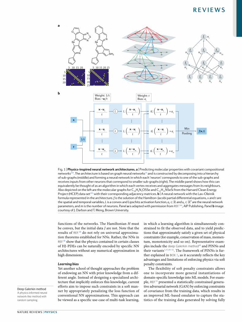
Some examplesFlow over an espresso cup. In the first example, we dis-cuss how to extract quantitative information on the 3D velocity and pressure fields above an espresso coffee cup140. The input data is based on a video of tempera-ture gradient (fig. 2). This is an example of the ‘hidden fluid mechanics’ introduced in ref.106. It is an ill- posed inverse problem as no boundary conditions or any other information are provided. Specifically, 3D visualizations obtained using tomographic background- oriented Schlieren (Tomo- BOS) imaging that measures density or temperature are used as input to a PINN, which seam-lessly integrates the visualization data and the flow and passive scalar governing equations, to infer the latent quantities. Here, the physical assumption is that of the Boussinesq approximation, which is valid if the density variation is relatively small.

The PINN uses the space and time coordinates as inputs and infers the velocity and pressure fields; it is trained by minimizing a loss function including a data mismatch of temperature and the residuals of the conservation laws (mass, momentum and energy). Independent experimental results from particle image velocimetry have verified that the Tomo- BOS/PINN approach is able to provide continuous, high- resolution and accurate 3D flow fields.

Aleatoric uncertaintyUncertainty due to the inherent randomness of data.

Epistemic uncertaintyUncertainty due to limited data and knowledge.

Arbitrary polynomial chaosA type of generalized polynomial chaos with measures defined by data.

Boussinesq approximationAn approximation used in gravity- driven flows, which ignores density differences except in the gravity term.

www.nature.com/natrevphys

R e v i e w s

0123456789();:

Physics- informed deep learning for 4D- flow MRI. Next, we discuss the use of PINNs in biophysics using real magnetic resonance imaging (MRI) data. Because it is non- invasive and proves a range of structural and phys-iological contrasts, MRI has become an indispensable tool for quantitative in- vivo assessment of blood flow and vascular function in clinical scenarios involving patients with cardiac and vascular disease. However, MRI measurements are often limited by the very coarse reso-lution and may be heavily corrupted by noise, leading to tedious and empirical workflows for reconstructing vascular topologies and associated flow conditions. Recent developments on physics- informed deep learn-ing can greatly enhance the resolution and information content of current MRI technologies, with a focus on 4D- flow MRI. Specifically, it is possible to construct DNNs that are constrained by the Navier–Stokes equa-tions in order to effectively de- noise MRI data and yield physically consistent reconstructions of the underlying velocity and pressure fields that ensure conservation of mass and momentum at an arbitrarily high spatial and temporal resolution. Moreover, the filtered veloc-ity fields can be used to identify regions of no- slip

flow, from which one can reconstruct the location and motion of the arterial wall and infer important quanti-ties of interest such as wall shear stresses, kinetic energy and dissipation (fig. 3). Taken together, these methods can considerably advance the capabilities of MRI tech-nologies in research and clinical scenarios. However, there are potential pitfalls related to the robustness of PINNs, especially in the presence of high signal- to- noise ratio in the MRI measurements and complex patterns in the underlying flow (for example, due to boundary layers, high- vorticity regions, transient turbulent bursts through a stenosis, tortuous branched vessels and so on). That said, under physiological conditions, blood flow is laminar, a regime under which current PINN models usually remain effective.

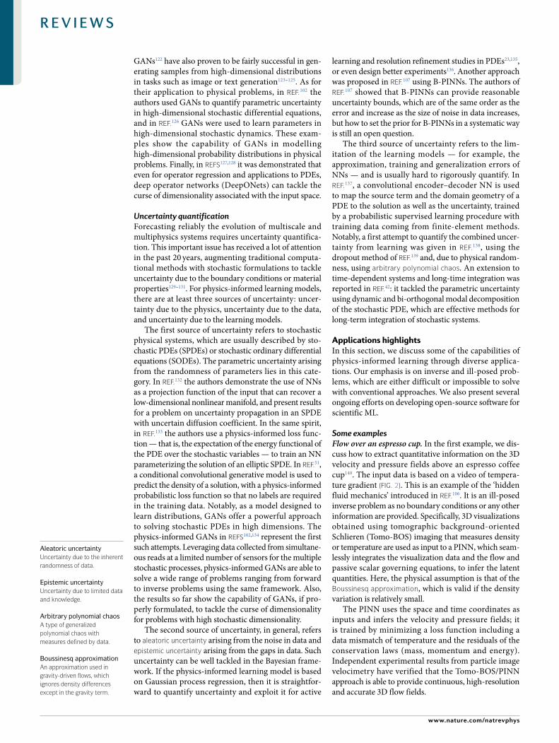
Uncovering edge plasma dynamics via deep learning from partial observations. Predicting turbulent trans-port on the edge of magnetic confinement fusion devices is a longstanding goal spanning several decades, cur-rently presenting significant uncertainties in the par-ticle and energy confinement of fusion power plants. In ref.141 it was demonstrated that PINNs can accurately

Tomo-BOS setup 3D temperature data

3D velocity 3D pressure

Physics-informedneural network

330325320315310305300295

0.340.300.260.220.180.140.100.060.02

0.0060.0050.0040.0030.0020.0010–0.001–0.002

(Kelvin)

(m s–1) (Pa)

yx

z

yx

z

yx

z

a

c

b

Fig. 2 | inferring the 3D flow over an espresso cup based using the Tomo-BOs imaging system and physics-informed neural networks (PiNNs). a | Six cameras are aligned around an espresso cup, recording the distortion of the dot- patterns in the panels placed in the background, where the distortion is caused by the density variation of the airflow above the espresso cup. The image data are acquired and processed with LaVision’s Tomographic BOS software (DaVis 10.1.1). b | 3D temperature field derived from the refractive index field and reconstructed based on the 2D images from all six cameras. c | Physics- informed neural network (PINN) inference of the 3D velocity field (left) and pressure field (right) from the temperature data. The Tomo- BOS experiment was performed by F. Fuest, Y. J. Jeon and C. Gray from LaVision. The PINN inference and visualization were performed by S. Cai and C. Li at Brown University. Image courtesy of S. Cai and C. Li, Brown University.

Nature reviews | Physics

R e v i e w s

0123456789();:

learn turbulent field dynamics consistent with the two- fluid theory from just partial observations of a synthetic plasma, for plasma diagnosis and model validation in challenging thermonuclear environments. figUre 4 dis-plays the turbulent radial electric field learned by PINNs from partial observations of a 3D synthetic plasma’s electron density and temperature141.

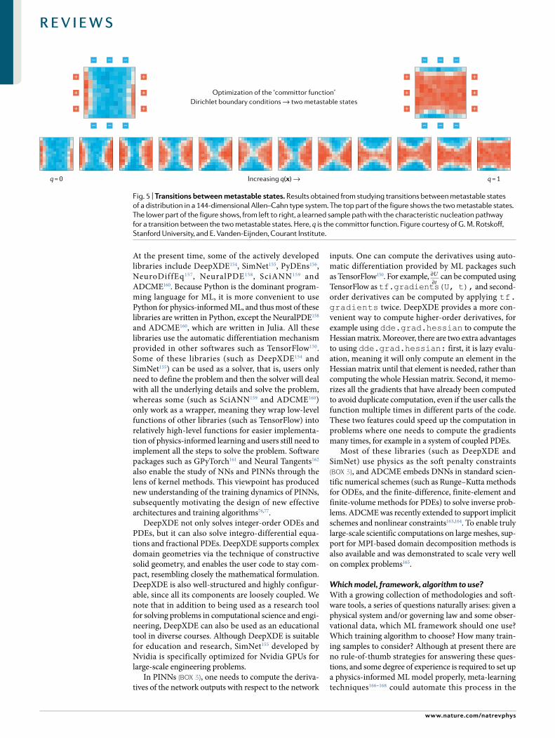
Studying transitions between metastable states of a dis-tribution. Next, we discuss how physics- informed learn-ing can be creatively used to tackle high- dimensional problems. In ref.142, the authors proposed to use physics- informed learning to study transitions between two metastable states of a high- dimensional probability distribution. In particular, an NN was used to represent the committor function, trained with a physics- informed loss function defined as the variational formula for the committor function combined with a soft penalty on the boundary conditions. Moreover, adaptive impor-tance sampling was used to sample rare events that dominate the loss function, which reduces the asymp-totic variance of the solution and improves gener-alization. Results for a probability distribution in a 144- dimensional Allen–Cahn type system are illustrated in fig. 5. Although these computational results suggest that this approach is effective for high- dimensional problems, the application of the method to more com-plicated systems and the selection of the NN architecture in adapting it to a given system remain challenging.

Thermodynamically consistent PINNs. The physics regularization generally pursued in PINNs admits an interpretation as a least- squares residual of point eval-uations using an NN basis. For hyperbolic problems involving shocks, where point evaluation of the solu-tion is ill- defined, it is natural to consider alternative physics stabilization requiring reduced regularity. The control volume PINN (cvPINN) pursued by ref.143 generalizes traditional finite- volume schemes to deep learning settings. In addition to offering increased

accuracy due to reduced regularity requirements, con-nections to traditional finite- volume schemes allow nat-ural adaptation of total variation diminishing limiters and recovery of entropy solutions. This framework has allowed the estimation of black- box equations of state for shock hydrodynamics models appropriate for mate-rials such as metals. For scenarios such as phase tran-sitions at extreme pressures and temperatures, DNNs provide an ideal means of addressing unknown model form, whereas the finite- volume structure provided by cvPINNs allows enforcement of thermodynamic consistency.

Application to quantum chemistry. In some other appli-cations, researchers have also used the physics to design specific new architectures together with the principles of physics- informed learning. For example, in ref.32, a fermionic NN (FermiNet) was proposed for the ab initio calculation of the solution of the many- electron Schrödinger equation. FermiNet is a hybrid approach for embedding physics. First, to parameterize the wavefunc-tion, the NN has a specialized architecture that obeys Fermi–Dirac statistics: that is, it is anti- symmetric under the exchange of input electron states and the boundary conditions (decay at infinity). Second, the training of FermiNet is also physics- informed: that is, the loss function is set as the variational form of the energy expectation value, with the gradient estimated by the Monte Carlo method. Although the application of NNs leads to eliminating the basis- set extrapolation, which is a common source of error in computational quantum chemistry, the performance of NNs, in general, depends on many factors, including the architectures and opti-mization algorithms, which require further systematic investigation.

Application to material sciences. In applications to mate-rials, from the characterization of the material proper-ties to the non- destructive evaluation of their strength, physics- informed learning can play an important role

a b c d

Fig. 3 | Physics-informed filtering of in-vivo 4D-flow magnetic resonance imaging data of blood flow in a porcine descending aorta. Physics- informed neural network (PINN) models can be used to de- noise and reconstruct clinical magnetic resonance imaging (MRI) data of blood velocity, while constraining this reconstruction to respect the underlying physical laws of momentum and mass conservation, as described by the incompressible Navier–Stokes equations. Moreover, a trained PINN model has the potential to aid the automatic segmentation of the arterial wall

geometry and to infer important biomarkers such as blood pressure and wall shear stresses. a | Snapshot of in- vivo 4D- flow MRI measurements. b–d | A PINN reconstruction of the velocity field (panel b), pressure (panel c), arterial wall surface geometry and wall shear stresses (panel d). The 4D- flow MRI data were acquired by E. Hwuang and W. Witschey at the University of Pennsylvania. The PINN inference and visualization were performed by S. Wang, G. Kissas and P. Perdikaris at the University of Pennsylvania.

Committor functionA function used to study transitions between metastable states in stochastic systems.

Allen–Cahn type systemA type of system with both reaction and diffusion.

www.nature.com/natrevphys

R e v i e w s

0123456789();:

as the underlying problems are typically ill- posed and of inverse type. In ref.144, the authors introduced an optimized PINN trained to identify and precisely char-acterize a surface breaking crack in a metal plate. The PINN was supervised with realistic ultrasonic surface acoustic wave data acquired at a frequency of 5 MHz and physically informed by the acoustic wave equation, with the unknown wave speed function represented as an NN. A key element in training was the use of adaptive activation functions, which introduced new trainable hyper- parameters and substantially accelerated conver-gence even in the presence of significant noise in the data. An alternative approach to introducing physics into ML is through a multi- fidelity framework as in ref.64 for extracting mechanical properties of 3D- printed materi-als via instrumented indentation. By solving the inverse problem of depth- sensing indentation, the authors could determine the elastoplastic properties of 3D- printed tita-nium and nickel alloys. In this framework, a composite NN consisting of two ResNets was used. One is a low- fidelity ResNet that uses synthetic data (a lot of finite- element simulations) and the other is a high- fidelity ResNet that uses as input the sparse experimental data and the output of the low- fidelity data. The objective was to discover the nonlinear correlation function between the low- and high- fidelity data, and subsequently predict the modulus of elasticity and yield stress at high fidelity. The results reported in ref.64 show impressive performance of the multi- fidelity framework, reducing the inference error for the yield stress from over 100% with existing techniques to lower than 5% with the multi- fidelity framework.

Application to molecular simulations. In ref.145, an NN architecture was proposed to represent the potential energy surfaces for molecular dynamics simulations, where the translational, rotational and permutational

symmetry of the molecular system is preserved with proper pre- processing. Such an NN representation could be further improved in deep potential molecular dynam-ics (DeePMD)146. With traditional artificially designed potential energy functions replaced by the NN trained with data from ab initio simulations, DeePMD achieves an ab initio level of accuracy at a cost that scales linearly with the system size. In ref.147, the limit of molecular dynamics simulations was pushed with ab initio accu-racy to simulating more than 1- ns- long trajectories of over 100 million atoms per day, using a highly opti-mized code for DeePMD on the Summit supercomputer. Before this work, molecular dynamics simulations with ab initio accuracy were performed in systems with up to 1 million atoms147,148.

Application to geophysics. Physics- informed learning has also been applied to various geophysical inverse problems. The work in ref.71 estimates subsurface properties, such as rock permeability and porosity, from seismic data by coupling NNs with full- waveform inversion, subsurface flow processes and rock physics models. Furthermore, in ref.149, it was demonstrated that by combining DNNs and numerical PDE solvers as we discussed in the section on hybrid approaches, physics- informed learning is capable of solving a wide class of seismic inversion problems, such as velocity esti-mation, fault rupture imaging, earthquake location and source–time function retrieval.

SoftwareTo implement PINNs efficiently, it is advantageous to build new algorithms based on the current ML libraries, such as TensorFlow150, PyTorch151, Keras152 and JAX153. Several software libraries specifically designed for physics-informed ML have been developed and are con-tributing to the rapid development of the field (TABLe 1).

ϕ (V)

x (cm)

y (c

m)

y (c

m)

0

0

–0.5

0.5

1.0

–1.00.5 1.0 2.0 3.01.5 2.5

0 0.5 1.0 2.0 3.01.5 2.5

–376,700

300

200

100

–376,800

–376,900

–377,000

x (cm)

0

–0.5

0.5

1.0

–1.0

Er (V m–1)

ϕ (V)Er (V m–1)

y (c

m)

0 0.5 1.0 2.0 3.01.5 2.5

20,000

10,000

0

x (cm)

0

–0.5

0.5

1.0

–1.0

y (c

m)

0 0.5 1.0 2.0 3.01.5 2.5

20,000

10,000

0

x (cm)

0

–0.5

0.5

1.0

–1.0

ne (m–3)

Te (eV)

y (c

m)

0 0.5 1.0 2.0 3.01.5 2.5

6

2345

x (cm)

0

–0.5

0.5

1.0

–1.0

y (c

m)

0 0.5 1.0 2.0 3.01.5 2.5

60

40

20

x (cm)

0

–0.5

0.5

1.0

–1.0

1 × 1018

Fig. 4 | Uncovering edge plasma dynamics. One of the most intensely studied aspects of magnetic confinement fusion is edge plasma behaviour, which is critical to reactor performance and operation. The drift- reduced Braginskii two- fluid theory has for decades been widely used to model edge plasmas, with varying success. Using a 3D magnetized two- fluid model, physics- informed neural networks (PINNs) can be used to accurately reconstruct141 the unknown turbulent electric field (middle panel) and underlying electric potential (right panel), directly from partial observations

of the plasma’s electron density and temperature from a single test discharge (left panel). The top row shows the reference target solution, while the bottom row depicts the PINN model’s prediction. These 2D synthetic measurements of electron density and temperature over the duration of a single plasma discharge constitute the only physical dynamics observed by the PINNs from the 3D collisional plasma exhibiting blob- like filaments. ϕ, electric potential; Er, electric field; ne, electron density; Te, electron temperature. Figure courtesy of A. Matthews, MIT.

Nature reviews | Physics

R e v i e w s

0123456789();:

At the present time, some of the actively developed libraries include DeepXDE154, SimNet155, PyDEns156, NeuroDiffEq157, NeuralPDE158, SciANN159 and ADCME160. Because Python is the dominant program-ming language for ML, it is more convenient to use Python for physics- informed ML, and thus most of these libraries are written in Python, except the NeuralPDE158 and ADCME160, which are written in Julia. All these libraries use the automatic differentiation mechanism provided in other softwares such as TensorFlow150. Some of these libraries (such as DeepXDE154 and SimNet155) can be used as a solver, that is, users only need to define the problem and then the solver will deal with all the underlying details and solve the problem, whereas some (such as SciANN159 and ADCME160) only work as a wrapper, meaning they wrap low- level functions of other libraries (such as TensorFlow) into relatively high- level functions for easier implementa-tion of physics- informed learning and users still need to implement all the steps to solve the problem. Software packages such as GPyTorch161 and Neural Tangents162 also enable the study of NNs and PINNs through the lens of kernel methods. This viewpoint has produced new understanding of the training dynamics of PINNs, subsequently motivating the design of new effective architectures and training algorithms76,77.

DeepXDE not only solves integer- order ODEs and PDEs, but it can also solve integro- differential equa-tions and fractional PDEs. DeepXDE supports complex domain geometries via the technique of constructive solid geometry, and enables the user code to stay com-pact, resembling closely the mathematical formulation. DeepXDE is also well- structured and highly configur-able, since all its components are loosely coupled. We note that in addition to being used as a research tool for solving problems in computational science and engi-neering, DeepXDE can also be used as an educational tool in diverse courses. Although DeepXDE is suitable for education and research, SimNet155 developed by Nvidia is specifically optimized for Nvidia GPUs for large- scale engineering problems.

In PINNs (Box 3), one needs to compute the deriva-tives of the network outputs with respect to the network

inputs. One can compute the derivatives using auto-matic differentiation provided by ML packages such as TensorFlow150. For example, U

t∂∂

can be computed using TensorFlow as tf.gradients(U, t), and second- order derivatives can be computed by applying tf.gradients twice. DeepXDE provides a more con-venient way to compute higher- order derivatives, for example using dde.grad.hessian to compute the Hessian matrix. Moreover, there are two extra advantages to using dde.grad.hessian: first, it is lazy evalu-ation, meaning it will only compute an element in the Hessian matrix until that element is needed, rather than computing the whole Hessian matrix. Second, it memo-rizes all the gradients that have already been computed to avoid duplicate computation, even if the user calls the function multiple times in different parts of the code. These two features could speed up the computation in problems where one needs to compute the gradients many times, for example in a system of coupled PDEs.

Most of these libraries (such as DeepXDE and SimNet) use physics as the soft penalty constraints (Box 3), and ADCME embeds DNNs in standard scien-tific numerical schemes (such as Runge–Kutta methods for ODEs, and the finite- difference, finite- element and finite- volume methods for PDEs) to solve inverse prob-lems. ADCME was recently extended to support implicit schemes and nonlinear constraints163,164. To enable truly large- scale scientific computations on large meshes, sup-port for MPI- based domain decomposition methods is also available and was demonstrated to scale very well on complex problems165.

Which model, framework, algorithm to use?With a growing collection of methodologies and soft-ware tools, a series of questions naturally arises: given a physical system and/or governing law and some obser-vational data, which ML framework should one use? Which training algorithm to choose? How many train-ing samples to consider? Although at present there are no rule- of- thumb strategies for answering these ques-tions, and some degree of experience is required to set up a physics- informed ML model properly, meta- learning techniques166–168 could automate this process in the

Increasing q(x) → q = 1q = 0

Optimization of the ‘committor function’Dirichlet boundary conditions → two metastable states

Fig. 5 | Transitions between metastable states. Results obtained from studying transitions between metastable states of a distribution in a 144- dimensional Allen–Cahn type system. The top part of the figure shows the two metastable states. The lower part of the figure shows, from left to right, a learned sample path with the characteristic nucleation pathway for a transition between the two metastable states. Here, q is the committor function. Figure courtesy of G. M. Rotskoff, Stanford University, and E. Vanden- Eijnden, Courant Institute.

www.nature.com/natrevphys

R e v i e w s

0123456789();:

future. The choices intimately depend on the specific task that needs to be tackled. In terms of providing a high- level taxonomy, we note that PINNs are typically used to infer a deterministic function that is compatible with an underlying physical law when a limited number of observations is available (either initial/boundary con-ditions or other measurements). The underlying archi-tecture of a PINNs model is determined by the nature of a given problem: multi- layer perceptron architectures are generally applicable but do not encode any special-ized inductive biases, convolutional NN architectures are suitable for gridded 2D domains, Fourier feature networks are suitable for PDEs whose solution exhib-its high frequencies or periodic boundaries, and recur-rent architectures are suitable for non- Markovian and time- discrete problems. Moreover, probabilistic variants of PINNs can also be used to infer stochastic processes that can allow capturing epistemic/model uncertainty (via Bayesian inference or frequentist ensembles) or aleatoric uncertainty (via generative models such as variational auto- encoders and GANs). However, the DeepONet framework can be used to infer an operator (instead of a function). In DeepONet, the choice of the underlying architecture can also vary depending on the nature of available data, such as scattered sensor measurements (multi- layer perceptron), images (convo-lutional NNs) or time series (recurrent NNs). In all the aforementioned cases, the required sample complexity is typically not known a priori and is generally determined by: the strength of inductive biases used in the architec-ture; the compatibility between the observed data, and the underlying physical law used as regularization; and the complexity of the underlying function or operator to be approximated.

Current limitationsMultiscale and multiphysics problemsDespite the recent success of physics- informed learning across a range of applications, multiscale and multi-physics problems require further developments. For example, fully connected NNs have difficulty learning high- frequency functions, a phenomenon referred to in the literature as the ‘F- principle’169 or ‘spectral bias’170. Additional work171,172 rigorously proved the existence of frequency bias in DNNs and derived convergence rates

of training as a function of target frequency. Moreover, high- frequency features in the target solution generally result in steep gradients, and thus PINN models often struggle to penalize accurately the PDE residuals45. As a consequence, for multiscale problems, the networks struggle to learn high- frequency components and often may fail to train76,173. To address the challenge of learn-ing high- frequency components, one needs to develop new techniques to aid the network learning, such as domain decomposition105, Fourier features174 and multiscale DNN45,175. However, learning multiphysics simultaneously could be computationally expensive. To address this issue, one may first learn each physics sep-arately and then couple them together. In the method of DeepM&M for the problems of electro- convection60 and hypersonics61, several DeepONets were first trained for each field separately and subsequently learned the coupled solutions through either a parallel or a serial DeepM&M architecture using supervised learning based on additional data for a specific multiphysics problem. It is also possible to learn the physics at a coarse scale by using the fine- scale simulation data only in small domains176.

Currently in NN- based ML methods, the physics- informed loss functions are mainly defined in a point- wise way. Although NNs with such loss functions can be successful in some high- dimensional problems, they may also fail in some special low- dimensional cases, such as the diffusion equation with non- smooth conductivity/permeability177.

New algorithms and computational frameworksPhysics- informed ML models often involve training large- scale NNs with complicated loss functions, which generally consist of multiple terms and thus are highly non- convex optimization problems178. The terms in the loss function may compete with each other dur-ing training. Consequently, the training process may not be robust and sufficiently stable, and thus conver-gence to the global minimum cannot be guaranteed179. To resolve this issue, one needs to develop more robust NN architectures and training algorithms for diverse applications. For example, refs76,77,173 have identified two fundamental weaknesses of PINNs, relating spec-tral bias170 to a discrepancy in the convergence rate of different components in a PINN loss function. The latter is manifested by training instabilities leading to vanishing back- propagated gradients. As discussed in these refs76,77,173, these pathologies can be mitigated by designing appropriate model architectures and new training algorithms for PINNs. Also, ref.104 used the weak form of the PDE and hp- refinement via decompo-sition to enhance the approximation capability of net-works. Other examples include adaptively modifying the activation functions180 or sampling the data points and the residual evaluation points during training181, which accelerate convergence and improve the performance of physics- informed models. Moreover, the design of effec-tive NN architectures is currently done empirically by users, which could be very time- consuming. However, emerging meta- learning techniques can be used to auto-mate this search166–168. What is interesting here is that

Table 1 | Major software libraries specifically designed for physics- informed machine learning

software name Usage Language Backend Ref.

DeepXDE Solver Python TensorFlow 154

SimNet Solver Python TensorFlow 155

PyDEns Solver Python TensorFlow 156

NeuroDiffEq Solver Python PyTorch 157

NeuralPDE Solver Julia Julia 158

SciANN Wrapper Python TensorFlow 159

ADCME Wrapper Julia TensorFlow 160

GPyTorch Wrapper Python PyTorch 161

Neural Tangents Wrapper Python JAX 162

hp- refinementDual refinement of the mesh by increasing either the number of subdomains or the approximations degree.

Nature reviews | Physics

R e v i e w s

0123456789();:

the architecture may be changing as the bifurcation parameters of the system (such as the Reynolds num-ber) increase. The training and optimization of deep learning models is expensive, and it is crucial to speed up the learning, for instance through transfer learning via DeepONets as in the example of crack propagation reported in ref.182. In addition, scalable and parallel training algorithms should be developed by using hard-ware like GPUs and tensor processing units, using both data- parallel and model- parallel algorithms.

Unlike classic classification or regression tasks, where the first- order derivative is required for gradient descent, physics- informed ML usually involves higher- order derivatives. Currently, their efficient evaluation is not well supported in popular software frameworks such as TensorFlow and PyTorch. An ML software library that is more efficient for computing high- order deriv-atives (for example, via Taylor- mode automatic differ-entiation)183,184 could greatly reduce the computational cost and boost the application of physics- informed ML across different disciplines. In addition to integer- order derivatives, other operators such as integral operators and even fractional- order derivatives103 are very useful in physics- informed learning.

Data generation and benchmarksIn the ML community dealing with imaging, speech and natural language processing problems, the use of standard benchmarks is very common in order to assess algorithm improvement, reproducibility of results, and expected computational cost. The UCI Machine Learning Repository185, which was created over three decades ago, is a collection of databases and data generators that are often used to compare the relative performance of new algorithms. Currently, they also include experimental data sets in the physical sciences, for example noise gen-erated by an aerofoil, ocean temperature and current measurements related to El Niño, and hydrodynamic resistance related to different yacht designs. These data sets are useful and are intended for data- driven mod-elling in ML, but in principle they can also be used for benchmarking physics- informed ML methods, assuming that proper parameterized physical models can be explic-itly included in the databases. However, in many differ-ent applications in physics and chemistry, full- field data are required, which cannot be obtained experimentally (for example in density- functional theory and molecular dynamics simulation or in direct numerical simulations of turbulence), and which tax computational resources heavily both in terms of time and memory. Hence, care-ful consideration should be given to how to make these data publicly available, how to curate such valuable data, and how to include the physical models and all param-eters required for the generation of these databases. In addition, it will take a concerted effort by research-ers to design meaningful benchmarks that test accuracy and speed- up of the new proposed physics- informed algorithms, which is a non- trivial task. Indeed, even for the aforementioned imaging and other established ML applications, there are still new developments on refining existing benchmarks and metrics, especially if software and hardware considerations are also factored in such

evaluations (for example, an in- depth analysis for image recognition)186. In physical systems, these difficulties are exacerbated by the fact that the aim is to predict dynam-ics, and it will be complicated, for example, to determine how to capture or identify bifurcations in dynamical systems and chaotic states.

However, new metrics such as the valid- time- prediction introduced in ref.187 may be appropriate and offer a promising direction to follow.

New mathematicsDespite the empirical success of physics- informed learning models, little is known about the theoretical foundation of such constrained NNs. A new theory is required to rigorously analyse the capabilities and lim-itations of physics- informed learning (for example, the learning capacity of NNs). More specifically, a funda-mental question is: can a network find solutions to PDE via gradient- based optimization? To answer this ques-tion, one should analyse the total error in deep learning, which can be decomposed into three types of errors: approximation error (can a network approximate a solu-tion to PDE with any accuracy?), optimization error (can one attain zero or very small training loss?) and gener-alization error (does smaller training error mean more accurate predicted solution?). It is important to analyse the well- posedness of the problem and the stability and convergence in terms of these errors. In particular, if the operator to be solved is (possibly partially) learned by the data themselves, establishing how well- posed any problem involving this operator is becomes an exciting mathematical challenge. The challenge is exacerbated when the initial/boundary/internal conditions are provided themselves as (possibly uncertain) data. This well- posedness issue must be analysed mathematically, aided by ML computational exploration.

The first mathematical analysis for PINNs in solv-ing forward problems appeared in ref.188, where the Hölder regularization was introduced to control generaliza-tion error. Specifically, ref.188 analysed the second- order linear elliptic and parabolic type PDEs and proved the consistency of results. References189,190 used quadrature points in the formulation of the loss and provided an abstract error estimate for both forward and inverse prob-lems. However, no convergence results were reported, as the use of quadrature points does not quantify the generalization error. In subsequent work, ref.191 studied linear PDEs and proposed an abstract error estimates framework for analysing both PINNs7 and variational PINNs104,192. Based on the compactness assumptions and the norm equivalence relations, sufficient condi-tions for convergence to the underlying PDE solution were obtained. The generalization error was handled by the rademacher complexity. For the continuous loss for-mulation, refs49,193–195 derived some error estimates based on the continuous loss formulations of PINNs. Although known error bounds involved with continuous norms (from PDE literature) may serve as error bounds for (continuous) PINNs, data samples have to be taken into account to quantify the generalization error.

In general, NNs are trained by gradient- based optimi-zation methods, and a new theory should be developed

Hölder regularizationA regularization term associated with Hölder constants of differential equations that controls the derivatives of neural networks.

Rademacher complexityA quantity that measures richness of a class of real- valued functions with respect to a probability distribution.

www.nature.com/natrevphys

R e v i e w s

0123456789();:

to better understand their training dynamics (gradient descent, stochastic gradient descent, Adam196 and so on). In ref.197, over- parameterized two- layer networks were analysed, and it was proved that the convergence of gradient descent for second- order linear PDEs, but the boundary conditions were not included in the analysis.

In ref.76, the neural tangent kernel theory198 was extended to PINNs, and it was shown that the training dynamics of PINNs sometimes can be regarded as a kernel regression as the width of network goes to infinity.

It is also helpful to understand the training process of networks by visualizing the landscape of loss func-tion of different formulations (strong form, weak form and so on). Furthermore, more methods are being rap-idly developed nowadays, and thus it is also important to understand the equivalence between models and the equivalence between different loss functions with different norms.

Analysing the physics- informed ML models based on rigorous theory calls for a fruitful synergy between deep learning, optimization, numerical analysis and PDE theory that not only has the potential to lead to more robust and effective training algorithms, but also to build a solid foundation for this new generation of computational methods.

OutlookPhysics- informed learning integrates data and math-ematical models seamlessly even in noisy and high- dimensional contexts, and can solve general inverse problems very effectively. Here, we have summarized some of the key concepts in Boxes 1–3 and provided references to frameworks and open- source software for the interested reader to have a head start in exploring physics- informed learning. We also discussed current capabilities and limitations and highlighted diverse applications from fluid dynamics to biophysics, plasma physics, transition between metastable states and other applications in materials. Next, we present possible new directions for applications of physics- informed learn-ing machines as well as research directions that will contri bute to their faster training, more accurate pre-dictions, and better interpretability for diverse physics applications and beyond.

Although there have been tools like TensorBoard to visualize the model graph, track the variables and metrics, and so on, for physical problems, extended requirements may include incorporating multiple physics and complicated geometry domain into the learning algorithm, visualizing the solution field (even high- dimensional ones), as in traditional computing platforms such as FEniCS199, OpenFOAM10 and others. A user- friendly, graph- based ML development environ-ment that can address the above issues could help more practitioners to develop physics- informed ML algorithms for applications to a wide range of diverse physical problems.

Future directionsDigital twins. ‘Digital twins’, a concept first put forth by General Electric to describe the digital copy of an engine manufactured in their factories, are now

becoming a reality in a number of industries. By assim-ilating real measurements to calibrate computational models, a digital twin aims to replicate the behaviour of a living or non- living physical entity in silico. Before these emerging technologies can be translated into practice, a series of fundamental questions need to be addressed. First, observational data can be scarce and noisy, are often characterized by vastly hetero geneous data modalities (images, time series, lab tests, histo-rical data, clinical records and so on), and may not be directly available for certain quantities of interest. Second, physics- based computational models heavily rely on tedious pre- processing and calibration proce-dures (such as mesh generation or calibration of initial and boundary conditions) that typically have a consid-erable cost, hampering their use in real- time decision- making settings. Moreover, physical models of many complex natural systems are, at best, ‘partially’ known as conservation laws, and do not provide a closed sys-tem of equations unless appropriate constitutive laws are postulated. Thanks to its natural capability of blend-ing physical models and data as well as the use of auto-matic differentiation that removes the need for mesh generation, physics- informed learning is well placed to become an enabling catalyst in the emerging era of digital twins.

Data and model transformations, fusion and inter-pretability. As the interactions between physics- based modelling and ML intensify, one will encounter — with increasing frequency — situations in which different researchers arrive at different data- driven models of the same phenomenon, even if they use the same training data (or equally informative data, observed through dif-ferent sensors). For example, two research groups using the same or equivalent alternative data may end up having differently trained networks (differently learned latent spaces, differently learned operators) even though their predictions are practically indistinguishable on the training set. Recognizing that there is often no unique physical interpretation of an observed phenomenon, here we foresee the importance of building ML- based transformations between predictive models, models at different fidelities, and theories, that are one- to- one (transformable, ‘dual’, calibratable) to each other in a verifiable manner. Researchers are increasingly discov-ering such transformations (for example from nonlinear dynamics to the corresponding Koopman model; from a Poisson system to the corresponding Hamiltonian one; from Nesterov iterations to their corresponding ODEs) in a data- driven manner. Such transformations will allow data and models to be systematically fused. Transformations between the ML latent space fea-tures and the physically interpretable observables, or ML- learned operators and closed- form equations, will obviously bolster the interpretability of the ML model. Ultimately, one needs to test how far these transforma-tions generalize: for what range of observations an ML model can be mapped to a different ML model, or to a physical model, and what the generalization limit is, beyond which they cannot be transformed or calibrated to each other.

Koopman modelLinear model of a (nonlinear) dynamical system obtained via a Koopman operator theory.

Nesterov iterationsiterations of an algorithm for the numerical computation of equilibria.

Nature reviews | Physics

R e v i e w s

0123456789();:

Searching for intrinsic variables and emergent, useful representations. Most of the current physics- informed ML methods follow this paradigm: first define a set of (humanly interpretable) observables/variables; then col-lect data; formulate the physics completely or incom-pletely using a ‘reasonable’ dictionary of operators based on the chosen observables; and finally apply the learning algorithm of choice. An emerging paradigm fuelled by advances in ML is to use observations and learning methods to automatically determine good/intrinsic variables and to also find useful or informative physical model formulations. Stepping beyond princi-pal component analysis, manifold learning techniques (from isoMAP to t- sNe and diffusion maps) and their deep learning counterparts of generative models and (possibly variational) auto- encoders are used to embed raw observations in reduced, mathematically useful latent spaces, in which evolution rules can be learned. Remarkably, these useful representations can go beyond embedding the relevant features, the dependent vari ables in a PDE. For spatiotemporally disordered data, one can also create ML- driven emergent spaces200,201 in terms of ML- learned independent variables: emergent ‘space- times’ in which the model operators will be learned. The DARPA Shredder Challenge202 of 2011 recreated space by effectively solving puzzles: documents shredded using a variety of paper shredding techniques. Today, disor-ganized spatiotemporal observations can be embedded in informative ‘independent variable’ emergent spaces. For example, evolution operators in the form of PDEs or

SODEs will then be learned in terms of these new, emer-gent space — even possibly time — independent vari-ables; there is a direct analogy here with the discussion of emergent space- time in modern physics203.

Such new paradigms could play a critical role in design optimization or in building a digital twin for complicated systems, even systems of systems, where humans can hardly write down a neat physical formu-lation in closed form. Moreover, instead of collecting data from experiments first and then performing the learning algorithm, it becomes important to integrate both in an active learning framework. In this way, a judicious selection of new and informative data can be aided by exploiting the geometry of latent space of the learning algorithms, while the algorithms can gradually improve the choice of latent space descriptors, as well as the mathematical formulation governing the physics, so as to yield realistic predictions as the experiments go on.

Ultimately, the main element we see changing is what we mean by ‘understanding’. Up to now, understanding meant that, say, each term in a PDE had a physical or mechanistic interpretation operated on some physically meaningful observables (dependent variables) and also operated in terms of some physically meaningful space/time (independent) variables. Now, it becomes possi-ble to make accurate predictions without this type of mechanistic understanding — and ‘understanding’ is something that may be redefined in the process.

Published online xx xx xxxx

ISOMAPA nonlinear dimensionality reduction technique for embedding intrinsically low- dimensional data from high- dimensional representations to lower- dimensional spaces.

t- SNEt- distributed stochastic neighbour embedding. A nonlinear dimensionality reduction technique for embedding intrinsically low- dimensional data from high- dimensional representations to lower- dimensional spaces.

Diffusion mapsA nonlinear dimensionality reduction technique for embedding intrinsically low- dimensional data from high- dimensional representations to lower- dimensional spaces.

1. Hart, J. K. & Martinez, K. Environmental sensor networks: a revolution in the earth system science? Earth Sci. Rev. 78, 177–191 (2006).

2. Kurth, T. et al. Exascale deep learning for climate analytics (IEEE, 2018).

3. Reddy, D. S. & Prasad, P. R. C. Prediction of vegetation dynamics using NDVI time series data and LSTM. Model. Earth Syst. Environ. 4, 409–419 (2018).

4. Reichstein, M. et al. Deep learning and process understanding for data- driven earth system science. Nature 566, 195–204 (2019).

5. Alber, M. et al. Integrating machine learning and multiscale modeling — perspectives, challenges, and opportunities in the biological, biomedical, and behavioral sciences. NPJ Digit. Med. 2, 1–11 (2019).

6. Iten, R., Metger, T., Wilming, H., Del Rio, L. & Renner, R. Discovering physical concepts with neural networks. Phys. Rev. Lett. 124, 010508 (2020).

7. Raissi, M., Perdikaris, P. & Karniadakis, G. E. Physics- informed neural networks: a deep learning framework for solving forward and inverse problems involving nonlinear partial differential equations. J. Comput. Phys. 378, 686–707 (2019).

8. Schmidt, M. & Lipson, H. Distilling free- form natural laws from experimental data. Science 324, 81–85 (2009).

9. Brunton, S. L., Proctor, J. L. & Kutz, J. N. Discovering governing equations from data by sparse identification of nonlinear dynamical systems. Proc. Natl Acad. Sci. USA 113, 3932–3937 (2016).

10. Jasak, H. et al. OpenFOAM: A C++ library for complex physics simulations. Int. Workshop Coupled Methods Numer. Dyn. 1000, 1–20 (2007).

11. Plimpton, S. Fast parallel algorithms for short- range molecular dynamics. J. Comput. Phys. 117, 1–19 (1995).

12. Jia, X. et al. Physics- guided machine learning for scientific discovery: an application in simulating lake temperature profiles. Preprint at arXiv https://arxiv.org/ abs/2001.11086 (2020).

13. Lu, L., Jin, P., Pang, G., Zhang, Z. & Karniadakis, G. E. Learning nonlinear operators via DeepONet based on the universal approximation theorem of operators. Nat. Mach. Intell. 3, 218–229 (2021).

14. Kashefi, A., Rempe, D. & Guibas, L. J. A point- cloud deep learning framework for prediction of fluid flow fields on irregular geometries. Phys. Fluids 33, 027104 (2021).

15. Li, Z. et al. Fourier neural operator for parametric partial differential equations. in Int. Conf. Learn. Represent. (2021).

16. Yang, Y. & Perdikaris, P. Conditional deep surrogate models for stochastic, high- dimensional, and multi- fidelity systems. Comput. Mech. 64, 417–434 (2019).

17. LeCun, Y. & Bengio, Y. et al. Convolutional networks for images, speech, and time series. Handb. Brain Theory Neural Netw. 3361, 1995 (1995).

18. Mallat, S. Understanding deep convolutional networks. Phil. Trans. R. Soc. A 374, 20150203 (2016).

19. Bronstein, M. M., Bruna, J., LeCun, Y., Szlam, A. & Vandergheynst, P. Geometric deep learning: going beyond Euclidean data. IEEE Signal Process. Mag. 34, 18–42 (2017).

20. Cohen, T., Weiler, M., Kicanaoglu, B. & Welling, M. Gauge equivariant convolutional networks and the icosahedral CNN. Proc. Machine Learn. Res. 97, 1321–1330 (2019).

21. Owhadi, H. Multigrid with rough coefficients and multiresolution operator decomposition from hierarchical information games. SIAM Rev. 59, 99–149 (2017).

22. Raissi, M., Perdikaris, P. & Karniadakis, G. E. Inferring solutions of differential equations using noisy multi- fidelity data. J. Comput. Phys. 335, 736–746 (2017).

23. Raissi, M., Perdikaris, P. & Karniadakis, G. E. Numerical Gaussian processes for time- dependent and nonlinear partial differential equations. SIAM J. Sci. Comput. 40, A172–A198 (2018).

24. Owhadi, H. Bayesian numerical homogenization. Multiscale Model. Simul. 13, 812–828 (2015).

25. Hamzi, B. & Owhadi, H. Learning dynamical systems from data: a simple cross- validation perspective, part I: parametric kernel flows. Physica D 421, 132817 (2021).

26. Reisert, M. & Burkhardt, H. Learning equivariant functions with matrix valued kernels. J. Mach. Learn. Res. 8, 385–408 (2007).

27. Owhadi, H. & Yoo, G. R. Kernel flows: from learning kernels from data into the abyss. J. Comput. Phys. 389, 22–47 (2019).

28. Winkens, J., Linmans, J., Veeling, B. S., Cohen, T. S. & Welling, M. Improved semantic segmentation for histopathology using rotation equivariant convolutional networks. in Conf. Med. Imaging Deep Learn. (2018).

29. Bruna, J. & Mallat, S. Invariant scattering convolution networks. IEEE Trans. Pattern Anal. Mach. Intell. 35, 1872–1886 (2013).

30. Kondor, R., Son, H. T., Pan, H., Anderson, B. & Trivedi, S. Covariant compositional networks for learning graphs. Preprint at arXiv https://arxiv.org/abs/1801.02144 (2018).

31. Tai, K. S., Bailis, P. & Valiant, G. Equivariant transformer networks. Proc. Int. Conf. Mach. Learn. 97, 6086–6095 (2019).

32. Pfau, D., Spencer, J. S., Matthews, A. G. & Foulkes, W. M. C. Ab initio solution of the many- electron Schrödinger equation with deep neural networks. Phys. Rev. Res. 2, 033429 (2020).

33. Pun, G. P., Batra, R., Ramprasad, R. & Mishin, Y. Physically informed artificial neural networks for atomistic modeling of materials. Nat. Commun. 10, 1–10 (2019).

34. Ling, J., Kurzawski, A. & Templeton, J. Reynolds averaged turbulence modelling using deep neural networks with embedded invariance. J. Fluid Mech. 807, 155–166 (2016).

35. Jin, P., Zhang, Z., Zhu, A., Tang, Y. & Karniadakis, G. E. SympNets: intrinsic structure- preserving symplectic networks for identifying Hamiltonian systems. Neural Netw. 132, 166–179 (2020).

36. Lusch, B., Kutz, J. N. & Brunton, S. L. Deep learning for universal linear embeddings of nonlinear dynamics. Nat. Commun. 9, 4950 (2018).

37. Lagaris, I. E., Likas, A. & Fotiadis, D. I. Artificial neural networks for solving ordinary and partial differential equations. IEEE Trans. Neural Netw. 9, 987–1000 (1998).

38. Sheng, H. & Yang, C. PFNN: A penalty- free neural network method for solving a class of second- order boundary- value problems on complex geometries. J. Comput. Phys. 428, 110085 (2021).

www.nature.com/natrevphys

R e v i e w s

0123456789();:

39. McFall, K. S. & Mahan, J. R. Artificial neural network method for solution of boundary value problems with exact satisfaction of arbitrary boundary conditions. IEEE Transac. Neural Netw. 20, 1221–1233 (2009).

40. Beidokhti, R. S. & Malek, A. Solving initial- boundary value problems for systems of partial differential equations using neural networks and optimization techniques. J. Franklin Inst. 346, 898–913 (2009).

41. Lagari, P. L., Tsoukalas, L. H., Safarkhani, S. & Lagaris, I. E. Systematic construction of neural forms for solving partial differential equations inside rectangular domains, subject to initial, boundary and interface conditions. Int. J. Artif. Intell. Tools 29, 2050009 (2020).

42. Zhang, D., Guo, L. & Karniadakis, G. E. Learning in modal space: solving time- dependent stochastic PDEs using physics- informed neural networks. SIAM J. Sci. Comput. 42, A639–A665 (2020).

43. Dong, S. & Ni, N. A method for representing periodic functions and enforcing exactly periodic boundary conditions with deep neural networks. J. Comput. Phys. 435, 110242 (2021).

44. Wang, B., Zhang, W. & Cai, W. Multi- scale deep neural network (MscaleDNN) methods for oscillatory stokes flows in complex domains. Commun. Comput. Phys. 28, 2139–2157 (2020).

45. Liu, Z., Cai, W. & Xu, Z. Q. J. Multi- scale deep neural network (MscaleDNN) for solving Poisson–Boltzmann equation in complex domains. Commun. Comput. Phys. 28, 1970–2001 (2020).

46. Mattheakis, M., Protopapas, P., Sondak, D., Di Giovanni, M. & Kaxiras, E. Physical symmetries embedded in neural networks. Preprint at arXiv https://arxiv.org/abs/1904.08991 (2019).

47. Cai, W., Li, X. & Liu, L. A phase shift deep neural network for high frequency approximation and wave problems. SIAM J. Sci. Comput. 42, A3285–A3312 (2020).

48. Darbon, J. & Meng, T. On some neural network architectures that can represent viscosity solutions of certain high dimensional Hamilton- Jacobi partial differential equations. J. Comput. Phys. 425, 109907 (2021).

49. Sirignano, J. & Spiliopoulos, K. DGM: a deep learning algorithm for solving partial differential equations. J. Comput. Phys. 375, 1339–1364 (2018).

50. Kissas, G. et al. Machine learning in cardiovascular flows modeling: predicting arterial blood pressure from non- invasive 4D flow MRI data using physics- informed neural networks. Comput. Methods Appl. Mech. Eng. 358, 112623 (2020).

51. Zhu, Y., Zabaras, N., Koutsourelakis, P. S. & Perdikaris, P. Physics- constrained deep learning for high- dimensional surrogate modeling and uncertainty quantification without labeled data. J. Comput. Phys. 394, 56–81 (2019).

52. Geneva, N. & Zabaras, N. Modeling the dynamics of PDE systems with physics- constrained deep auto- regressive networks. J. Comput. Phys. 403, 109056 (2020).

53. Wu, J. L. et al. Enforcing statistical constraints in generative adversarial networks for modeling chaotic dynamical systems. J. Comput. Phys. 406, 109209 (2020).

54. Pfrommer, S., Halm, M. & Posa, M. Contactnets: learning of discontinuous contact dynamics with smooth, implicit representations. Preprint at arXiv https://arxiv.org/abs/2009.11193 (2020).

55. Erichson, N.B., Muehlebach, M. & Mahoney, M. W. Physics- informed autoencoders for Lyapunov- stable fluid flow prediction. Preprint at arXiv https://arxiv.org/ abs/1905.10866 (2019).

56. Shah, V. et al. Encoding invariances in deep generative models. Preprint at arXiv https://arxiv.org/abs/ 1906.01626 (2019).

57. Geneva, N. & Zabaras, N. Transformers for modeling physical systems. Preprint at arXiv https://arxiv.org/abs/2010.03957 (2020).

58. Li, Z. et al. Multipole graph neural operator for parametric partial differential equations. in Adv. Neural Inf. Process. Syst. (2020).

59. Nelsen, N. H. & Stuart, A. M. The random feature model for input–output maps between Banach spaces. Preprint at arXiv https://arxiv.org/abs/2005.10224 (2020).

60. Cai, S., Wang, Z., Lu, L., Zaki, T. A. & Karniadakis, G. E. DeepM&Mnet: inferring the electroconvection multiphysics fields based on operator approximation by neural networks. J. Comput. Phys. 436, 110296 (2020).

61. Mao, Z., Lu, L., Marxen, O., Zaki, T. A. & Karniadakis, G. E. DeepM&Mnet for hypersonics:

predicting the coupled flow and finite- rate chemistry behind a normal shock using neural- network approximation of operators. Preprint at arXiv https://arxiv.org/abs/2011.03349 (2020).

62. Meng, X. & Karniadakis, G. E. A composite neural network that learns from multi- fidelity data: application to function approximation and inverse PDE problems. J. Comput. Phys. 401, 109020 (2020).

63. Sirignano, J., MacArt, J. F. & Freund, J. B. DPM: a deep learning PDE augmentation method with application to large- eddy simulation. J. Comput. Phys. 423, 109811 (2020).

64. Lu, L. et al. Extraction of mechanical properties of materials through deep learning from instrumented indentation. Proc. Natl Acad. Sci. USA 117, 7052–7062 (2020).

65. Reyes, B., Howard, A. A., Perdikaris, P. & Tartakovsky, A. M. Learning unknown physics of non- Newtonian fluids. Preprint at arXiv https://arxiv.org/ abs/2009.01658 (2020).

66. Wang, W. & Gómez- Bombarelli, R. Coarse- graining auto- encoders for molecular dynamics. NPJ Comput. Mater. 5, 1–9 (2019).

67. Rico- Martinez, R., Anderson, J. & Kevrekidis, I. Continuous- time nonlinear signal processing: a neural network based approach for gray box identification (IEEE, 1994).

68. Xu, K., Huang, D. Z. & Darve, E. Learning constitutive relations using symmetric positive definite neural networks. Preprint at arXiv https://arxiv.org/abs/ 2004.00265 (2020).

69. Huang, D. Z., Xu, K., Farhat, C. & Darve, E. Predictive modeling with learned constitutive laws from indirect observations. Preprint at arXiv https://arxiv.org/abs/ 1905.12530 (2019).

70. Xu, K., Tartakovsky, A. M., Burghardt, J. & Darve, E. Inverse modeling of viscoelasticity materials using physics constrained learning. Preprint at arXiv https://arxiv.org/abs/2005.04384 (2020).

71. Li, D., Xu, K., Harris, J. M. & Darve, E. Coupled time- lapse full- waveform inversion for subsurface flow problems using intrusive automatic differentiation. Water Resour. Res. 56, e2019WR027032 (2020).

72. Tartakovsky, A., Marrero, C. O., Perdikaris, P., Tartakovsky, G. & Barajas- Solano, D. Physics- informed deep neural networks for learning parameters and constitutive relationships in subsurface flow problems. Water Resour. Res. 56, e2019WR026731 (2020).

73. Xu, K. & Darve, E. Adversarial numerical analysis for inverse problems. Preprint at arXiv https://arxiv.org/abs/1910.06936 (2019).

74. Yang, Y., Bhouri, M. A. & Perdikaris, P. Bayesian differential programming for robust systems identification under uncertainty. Proc. R. Soc. A 476, 20200290 (2020).

75. Rackauckas, C. et al. Universal differential equations for scientific machine learning. Preprint at arXiv https://arxiv.org/abs/2001.04385 (2020).

76. Wang, S., Yu, X. & Perdikaris, P. When and why PINNs fail to train: a neural tangent kernel perspective. Preprint at arXiv https://arxiv.org/abs/2007.14527 (2020).

77. Wang, S., Wang, H. & Perdikaris, P. On the eigenvector bias of Fourier feature networks: from regression to solving multi- scale PDEs with physics- informed neural networks. Preprint at arXiv https://arxiv.org/abs/ 2012.10047 (2020).

78. Pang, G., Yang, L. & Karniadakis, G. E. Neural- net-induced Gaussian process regression for function approximation and PDE solution. J. Comput. Phys. 384, 270–288 (2019).

79. Wilson, A. G., Hu, Z., Salakhutdinov, R. & Xing, E. P. Deep kernel learning. Proc. Int. Conf. Artif. Intell. Stat. 51, 370–378 (2016).

80. Owhadi, H. Do ideas have shape? Plato’s theory of forms as the continuous limit of artificial neural networks. Preprint at arXiv https://arxiv.org/abs/ 2008.03920 (2020).

81. Owhadi, H. & Scovel, C. Operator- Adapted Wavelets, Fast Solvers, and Numerical Homogenization: From a Game Theoretic Approach to Numerical Approximation and Algorithm Design (Cambridge Univ. Press, 2019).

82. Micchelli, C. A. & Rivlin, T. J. in Optimal Estimation in Approximation Theory (eds. Micchelli, C. A. & Rivlin, T. J.) 1–54 (Springer, 1977).

83. Sard, A. Linear Approximation (Mathematical Surveys 9, American Mathematical Society, 1963).

84. Larkin, F. Gaussian measure in Hilbert space and applications in numerical analysis. Rocky Mt. J. Math. 2, 379–421 (1972).

85. Sul’din, A. V. Wiener measure and its applications to approximation methods. I. Izv. Vyssh. Uchebn. Zaved. Mat. 3, 145–158 (1959).

86. Diaconis, P. Bayesian numerical analysis. Stat. Decision Theory Relat. Top. IV 1, 163–175 (1988).

87. Kimeldorf, G. S. & Wahba, G. A correspondence between Bayesian estimation on stochastic processes and smoothing by splines. Ann. Math. Stat. 41, 495–502 (1970).

88. Owhadi, H., Scovel, C. & Schäfer, F. Statistical numerical approximation. Not. Am. Math. Soc. 66, 1608–1617 (2019).

89. Tsai, Y. H. H., Bai, S., Yamada, M., Morency, L. P. & Salakhutdinov, R. Transformer dissection: a unified understanding of transformer’s attention via the lens of kernel. Preprint at arXiv https://arxiv.org/abs/ 1908.11775 (2019).

90. Kadri, H. et al. Operator- valued kernels for learning from functional response data. J. Mach. Learn. Res. 17, 1–54 (2016).

91. González- García, R., Rico- Martínez, R. & Kevrekidis, I. G. Identification of distributed parameter systems: a neural net based approach. Comput. Chem. Eng. 22, S965–S968 (1998).

92. Long, Z., Lu, Y., Ma, X. & Dong, B. PDE- Net: learning PDEs from data. Proc. Int. Conf. Mach. Learn. 80, 3208–3216 (2018).

93. He, J. & Xu, J. MgNet: a unified framework of multigrid and convolutional neural network. Sci. China Math. 62, 1331–1354 (2019).

94. He, K., Zhang, X., Ren, S. & Sun, J. Deep residual learning for image recognition (IEEE, 2016).

95. Rico- Martinez, R., Krischer, K., Kevrekidis, I., Kube, M. & Hudson, J. Discrete- vs. continuous- time nonlinear signal processing of Cu electrodissolution data. Chem. Eng. Commun. 118, 25–48 (1992).

96. Weinan, E. A proposal on machine learning via dynamical systems. Commun. Math. Stat. 5, 1–11 (2017).

97. Chen, T. Q., Rubanova, Y., Bettencourt, J. & Duvenaud, D. K. Neural ordinary differential equations. Adv. Neural Inf. Process. Syst. 31, 6571–6583 (2018).

98. Jia, J. & Benson, A. R. Neural jump stochastic differential equations. Adv. Neural Inf. Process. Syst. 32, 9847–9858 (2019).

99. Rico- Martinez, R., Kevrekidis, I. & Krischer, K. in Neural Networks for Chemical Engineers (ed. Bulsari, A. B.) 409–442 (Elsevier, 1995).

100. He, J., Li, L., Xu, J. & Zheng, C. ReLU deep neural networks and linear finite elements. J. Comput. Math. 38, 502–527 (2020).

101. Jagtap, A. D., Kharazmi, E. & Karniadakis, G. E. Conservative physics- informed neural networks on discrete domains for conservation laws: applications to forward and inverse problems. Comput. Methods Appl. Mech. Eng. 365, 113028 (2020).

102. Yang, L., Zhang, D. & Karniadakis, G. E. Physics- informed generative adversarial networks for stochastic differential equations. SIAM J. Sci. Comput. 42, A292–A317 (2020).

103. Pang, G., Lu, L. & Karniadakis, G. E. fPINNs: fractional physics- informed neural networks. SIAM J. Sci. Comput. 41, A2603–A2626 (2019).

104. Kharazmi, E., Zhang, Z. & Karniadakis, G. E. hp- VPINNs: variational physics- informed neural networks with domain decomposition. Comput. Methods Appl. Mech. Eng. 374, 113547 (2021).

105. Jagtap, A. D. & Karniadakis, G. E. Extended physics- informed neural networks (XPINNs): a generalized space- time domain decomposition based deep learning framework for nonlinear partial differential equations. Commun. Comput. Phys. 28, 2002–2041 (2020).

106. Raissi, M., Yazdani, A. & Karniadakis, G. E. Hidden fluid mechanics: learning velocity and pressure fields from flow visualizations. Science 367, 1026–1030 (2020).

107. Yang, L., Meng, X. & Karniadakis, G. E. B- PINNs: Bayesian physics- informed neural networks for forward and inverse PDE problems with noisy data. J. Comput. Phys. 415, 109913 (2021).

108. Wang, S. & Perdikaris, P. Deep learning of free boundary and Stefan problems. J. Comput. Phys. 428, 109914 (2020).

109. Spigler, S. et al. A jamming transition from under- to over- parametrization affects generalization in deep learning. J. Phys. A 52, 474001 (2019).

110. Geiger, M. et al. Scaling description of generalization with number of parameters in deep learning. J. Stat. Mech. Theory Exp. 2020, 023401 (2020).

Nature reviews | Physics

R e v i e w s

0123456789();:

111. Belkin, M., Hsu, D., Ma, S. & Mandal, S. Reconciling modern machine- learning practice and the classical bias–variance trade- off. Proc. Natl Acad. Sci. USA 116, 15849–15854 (2019).

112. Geiger, M. et al. Jamming transition as a paradigm to understand the loss landscape of deep neural networks. Phys. Rev. E 100, 012115 (2019).

113. Mei, S., Montanari, A. & Nguyen, P. M. A mean field view of the landscape of two- layer neural networks. Proc. Natl Acad. Sci. USA 115, E7665–E7671 (2018).

114. Mehta, P. & Schwab, D. J. An exact mapping between the variational renormalization group and deep learning. Preprint at arXiv https://arxiv.org/abs/ 1410.3831 (2014).

115. Stoudenmire, E. & Schwab, D. J. Supervised learning with tensor networks. Adv. Neural Inf. Process. Syst. 29, 4799–4807 (2016).

116. Choromanska, A., Henaff, M., Mathieu, M., Arous, G. B. & LeCun, Y. The loss surfaces of multilayer networks. Proc. Artif. Intell. Stat. 38, 192–204 (2015).

117. Poole, B., Lahiri, S., Raghu, M., Sohl- Dickstein, J. & Ganguli, S. Exponential expressivity in deep neural networks through transient chaos. Adv. Neural Inf. Process. Syst. 29, 3360–3368 (2016).

118. Yang, G. & Schoenholz, S. Mean field residual networks: on the edge of chaos. Adv. Neural Inf. Process. Syst. 30, 7103–7114 (2017).

119. Poggio, T., Mhaskar, H., Rosasco, L., Miranda, B. & Liao, Q. Why and when can deep — but not shallow — networks avoid the curse of dimensionality: a review. Int. J. Autom. Comput. 14, 503–519 (2017).

120. Grohs, P., Hornung, F., Jentzen, A. & Von Wurstemberger, P. A proof that artificial neural networks overcome the curse of dimensionality in the numerical approximation of Black–Scholes partial differential equations. Preprint at arXiv https://arxiv.org/abs/1809.02362 (2018).

121. Han, J., Jentzen, A. & Weinan, E. Solving high- dimensional partial differential equations using deep learning. Proc. Natl Acad. Sci. USA 115, 8505–8510 (2018).

122. Goodfellow, I. et al. Generative adversarial nets. Adv. Neural Inf. Process. Syst. 27, 2672–2680 (2014).

123. Brock, A., Donahue, J. & Simonyan, K. Large scale GAN training for high fidelity natural image synthesis. in Int. Conf. Learn. Represent. (2019).

124. Yu, L., Zhang, W., Wang, J. & Yu, Y. SeqGAN: sequence generative adversarial nets with policy gradient (AAAI Press, 2017).

125. Zhu, J.Y., Park, T., Isola, P. & Efros, A. A. Unpaired image- to-image translation using cycle- consistent adversarial networks (IEEE, 2017).

126. Yang, L., Daskalakis, C. & Karniadakis, G. E. Generative ensemble- regression: learning particle dynamics from observations of ensembles with physics- informed deep generative models. Preprint at arXiv https://arxiv.org/abs/2008.01915 (2020).

127. Lanthaler, S., Mishra, S. & Karniadakis, G. E. Error estimates for DeepONets: a deep learning framework in infinite dimensions. Preprint at arXiv https://arxiv.org/abs/2102.09618 (2021).

128. Deng, B., Shin, Y., Lu, L., Zhang, Z. & Karniadakis, G. E. Convergence rate of DeepONets for learning operators arising from advection–diffusion equations. Preprint at arXiv https://arxiv.org/abs/2102.10621 (2021).

129. Xiu, D. & Karniadakis, G. E. The Wiener–Askey polynomial chaos for stochastic differential equations. SIAM J. Sci. Comput. 24, 619–644 (2002).

130. Marzouk, Y. M., Najm, H. N. & Rahn, L. A. Stochastic spectral methods for efficient Bayesian solution of inverse problems. J. Comput. Phys. 224, 560–586 (2007).

131. Stuart, A. M. Inverse problems: a Bayesian perspective. Acta Numerica 19, 451 (2010).

132. Tripathy, R. K. & Bilionis, I. Deep UQ: learning deep neural network surrogate models for high dimensional uncertainty quantification. J. Comput. Phys. 375, 565–588 (2018).

133. Karumuri, S., Tripathy, R., Bilionis, I. & Panchal, J. Simulator- free solution of high- dimensional stochastic elliptic partial differential equations using deep neural networks. J. Comput. Phys. 404, 109120 (2020).

134. Yang, Y. & Perdikaris, P. Adversarial uncertainty quantification in physics- informed neural networks. J. Comput. Phys. 394, 136–152 (2019).

135. Raissi, M., Perdikaris, P. & Karniadakis, G. E. Machine learning of linear differential equations using Gaussian processes. J. Comput. Phys. 348, 683–693 (2017).

136. & Fan, D. et al. A robotic intelligent towing tank for learning complex fluid- structure dynamics. Sci. Robotics 4, eaay5063 (2019).

137. Winovich, N., Ramani, K. & Lin, G. ConvPDE- UQ: convolutional neural networks with quantified uncertainty for heterogeneous elliptic partial differential equations on varied domains. J. Comput. Phys. 394, 263–279 (2019).

138. Zhang, D., Lu, L., Guo, L. & Karniadakis, G. E. Quantifying total uncertainty in physics- informed neural networks for solving forward and inverse stochastic problems. J. Comput. Phys. 397, 108850 (2019).

139. Gal, Y. & Ghahramani, Z. Dropout as a Bayesian approximation: representing model uncertainty in deep learning. Proc. Int. Conf. Mach. Learn. 48, 1050–1059 (2016).

140. Cai, S. et al. Flow over an espresso cup: inferring 3-D velocity and pressure fields from tomographic background oriented Schlieren via physics- informed neural networks. J. Fluid Mech. 915 (2021).

141. Mathews, A., Francisquez, M., Hughes, J. & Hatch, D. Uncovering edge plasma dynamics via deep learning from partial observations. Preprint at arXiv https://arxiv.org/abs/2009.05005 (2020).

142. Rotskoff, G. M. & Vanden- Eijnden, E. Learning with rare data: using active importance sampling to optimize objectives dominated by rare events. Preprint at arXiv https://arxiv.org/abs/2008.06334 (2020).

143. Patel, R. G. et al. Thermodynamically consistent physics- informed neural networks for hyperbolic systems. Preprint at https://arxiv.org/abs/2012.05343 (2020).

144. Shukla, K., Di Leoni, P. C., Blackshire, J., Sparkman, D. & Karniadakis, G. E. Physics- informed neural network for ultrasound nondestructive quantification of surface breaking cracks. J. Nondestruct. Eval. 39, 1–20 (2020).

145. Behler, J. & Parrinello, M. Generalized neural- network representation of high- dimensional potential- energy surfaces. Phys. Rev. Lett. 98, 146401 (2007).

146. Zhang, L., Han, J., Wang, H., Car, R. & Weinan, E. Deep potential molecular dynamics: a scalable model with the accuracy of quantum mechanics. Phys. Rev. Lett. 120, 143001 (2018).

147. Jia, W. et al. Pushing the limit of molecular dynamics with ab initio accuracy to 100 million atoms with machine learning. Preprint at arXiv https://arxiv.org/abs/2005.00223 (2020).

148. Nakata, A. et al. Large scale and linear scaling DFT with the CONQUEST code. J. Chem. Phys. 152, 164112 (2020).

149. Zhu, W., Xu, K., Darve, E. & Beroza, G. C. A general approach to seismic inversion with automatic differentiation. Preprint at arXiv https://arxiv.org/abs/ 2003.06027 (2020).

150. Abadi, M. et al. Tensorflow: a system for large- scale machine learning. Proc. OSDI 16, 265–283 (2016).

151. Paszke, A. et al. PyTorch: an imperative style, high- performance deep learning library. Adv. Neural Inf. Process. Syst. 32, 8026–8037 (2019).

152. Chollet, F. et al. Keras — Deep learning library. Keras https://keras.io (2015).

153. Frostig, R., Johnson, M. J. & Leary, C. Compiling machine learning programs via high- level tracing. in Syst. Mach. Learn. (2018).

154. Lu, L., Meng, X., Mao, Z. & Karniadakis, G. E. DeepXDE: a deep learning library for solving differential equations. SIAM Rev. 63, 208–228 (2021).

155. Hennigh, O. et al. NVIDIA SimNet: an AI- accelerated multi- physics simulation framework. Preprint at arXiv https://arxiv.org/abs/2012.07938 (2020).

156. Koryagin, A., Khudorozkov, R. & Tsimfer, S. PyDEns: a Python framework for solving differential equations with neural networks. Preprint at arXiv https://arxiv.org/ abs/1909.11544 (2019).

157. Chen, F. et al. NeuroDiffEq: A python package for solving differential equations with neural networks. J. Open Source Softw. 5, 1931 (2020).

158. Rackauckas, C. & Nie, Q. DifferentialEquations.jl — a performant and feature- rich ecosystem for solving differential equations in Julia. J. Open Res. Softw. 5, 15 (2017).

159. Haghighat, E. & Juanes, R. SciANN: a Keras/TensorFlow wrapper for scientific computations and physics- informed deep learning using artificial neural networks. Comput. Meth. Appl. Mech. Eng. 373, 113552 (2020).

160. Xu, K. & Darve, E. ADCME: Learning spatially- varying physical fields using deep neural networks. Preprint at arXiv https://arxiv.org/abs/2011.11955 (2020).

161. Gardner, J. R., Pleiss, G., Bindel, D., Weinberger, K. Q. & Wilson, A. G. Gpytorch: blackbox matrix–matrix Gaussian process inference with GPU acceleration. Adv. Neural Inf. Process. Syst. 31, 7587–7597 (2018).

162. Novak, R. et al. Neural Tangents: fast and easy infinite neural networks in Python. in Conf. Neural Inform. Process. Syst. (2020).

163. Xu, K. & Darve, E. Physics constrained learning for data- driven inverse modeling from sparse observations. Preprint at arXiv https://arxiv.org/abs/2002.10521 (2020).

164. Xu, K. & Darve, E. The neural network approach to inverse problems in differential equations. Preprint at arXiv https://arxiv.org/abs/1901.07758 (2019).

165. Xu, K., Zhu, W. & Darve, E. Distributed machine learning for computational engineering using MPI. Preprint at arXiv https://arxiv.org/abs/2011.01349 (2020).

166. Elsken, T., Metzen, J. H. & Hutter, F. Neural architecture search: a survey. J. Mach. Learn. Res. 20, 1–21 (2019).

167. He, X., Zhao, K. & Chu, X. AutoML: a survey of the state- of-the- art. Knowl. Based Syst. 212, 106622 (2021).

168. Hospedales, T., Antoniou, A., Micaelli, P. & Storkey, A. Meta- learning in neural networks: a survey. Preprint at arXiv https://arxiv.org/abs/2004.05439 (2020).

169. Xu, Z.-Q. J., Zhang, Y., Luo, T., Xiao, Y. & Ma, Z. Frequency principle: Fourier analysis sheds light on deep neural networks. Commun. Comput. Phys. 28, 1746–1767 (2020).

170. Rahaman, N. et al. On the spectral bias of neural networks. Proc. Int. Conf. Mach. Learn. 97, 5301–5310 (2019).

171. Ronen, B., Jacobs, D., Kasten, Y. & Kritchman, S. The convergence rate of neural networks for learned functions of different frequencies. Adv. Neural Inf. Process. Syst. 32, 4761–4771 (2019).

172. Cao, Y., Fang, Z., Wu, Y., Zhou, D. X. & Gu, Q. Towards understanding the spectral bias of deep learning. Preprint at arXiv https://arxiv.org/abs/1912.01198 (2019).

173. Wang, S., Teng, Y. & Perdikaris, P. Understanding and mitigating gradient pathologies in physics- informed neural networks. Preprint at arXiv https://arxiv.org/abs/2001.04536 (2020).

174. Tancik, M. et al. Fourier features let networks learn high frequency functions in low dimensional domains. Adv. Neural Inf. Process. Syst. 33 (2020).

175. Cai, W. & Xu, Z. Q. J. Multi- scale deep neural networks for solving high dimensional PDEs. Preprint at arXiv https://arxiv.org/abs/1910.11710 (2019).

176. Arbabi, H., Bunder, J. E., Samaey, G., Roberts, A. J. & Kevrekidis, I. G. Linking machine learning with multiscale numerics: data- driven discovery of homogenized equations. JOM 72, 4444–4457 (2020).

177. Owhadi, H. & Zhang, L. Metric- based upscaling. Commun. Pure Appl. Math. 60, 675–723 (2007).

178. Blum, A. L. & Rivest, R. L. Training a 3-node neural network is NP- complete. Neural Netw. 5, 117–127 (1992).

179. Lee, J. D., Simchowitz, M., Jordan, M. I. & Recht, B. Gradient descent only converges to minimizers. Annu. Conf. Learn. Theory 49, 1246–1257 (2016).

180. Jagtap, A. D., Kawaguchi, K. & Em Karniadakis, G. Locally adaptive activation functions with slope recovery for deep and physics- informed neural networks. Proc. R. Soc. A 476, 20200334 (2020).

181. Wight, C. L. & Zhao, J. Solving Allen–Cahn and Cahn–Hilliard equations using the adaptive physics informed neural networks. Preprint at arXiv https://arXiv.org/abs/2007.04542 (2020).

182. Goswami, S., Anitescu, C., Chakraborty, S. & Rabczuk, T. Transfer learning enhanced physics informed neural network for phase- field modeling of fracture. Theor. Appl. Fract. Mech. 106, 102447 (2020).

183. Betancourt, M. A geometric theory of higher- order automatic differentiation. Preprint at arXiv https://arxiv.org/abs/1812.11592 (2018).

184. Bettencourt, J., Johnson, M. J. & Duvenaud, D. Taylor- mode automatic differentiation for higher- order derivatives in JAX. in Conf. Neural Inform. Process. Syst. (2019).

185. Newman, D, Hettich, S., Blake, C. & Merz, C. UCI repository of machine learning databases. ICS http://www.ics.uci.edu/~mlearn/MLRepository.html (1998).

186. Bianco, S., Cadene, R., Celona, L. & Napoletano, P. Benchmark analysis of representative deep neural

www.nature.com/natrevphys

R e v i e w s

0123456789();:

network architectures. IEEE Access 6, 64270–64277 (2018).

187. Vlachas, P. R. et al. Backpropagation algorithms and reservoir computing in recurrent neural networks for the forecasting of complex spatiotemporal dynamics. Neural Networks (2020).

188. Shin, Y., Darbon, J. & Karniadakis, G. E. On the convergence of physics informed neural networks for linear second- order elliptic and parabolic type PDEs. Commun. Comput. Phys. 28, 2042–2074 (2020).

189. Mishra, S. & Molinaro, R. Estimates on the generalization error of physics informed neural networks (PINNs) for approximating PDEs. Preprint at arXiv https://arxiv.org/abs/2006.16144 (2020).

190. Mishra, S. & Molinaro, R. Estimates on the generalization error of physics informed neural networks (PINNs) for approximating PDEs II: a class of inverse problems. Preprint at arXiv https://arxiv.org/ abs/2007.01138 (2020).

191. Shin, Y., Zhang, Z. & Karniadakis, G.E. Error estimates of residual minimization using neural networks for linear PDEs. Preprint at arXiv https://arxiv.org/abs/ 2010.08019 (2020).

192. Kharazmi, E., Zhang, Z. & Karniadakis, G. Variational physics- informed neural networks for solving partial differential equations. Preprint at arXiv https://arxiv.org/abs/1912.00873 (2019).

193. Jo, H., Son, H., Hwang, H. Y. & Kim, E. Deep neural network approach to forward- inverse problems. Netw. Heterog. Media 15, 247–259 (2020).

194. Guo, M. & Haghighat, E. An energy- based error bound of physics- informed neural network solutions in elasticity. Preprint at arXiv https://arxiv.org/abs/ 2010.09088 (2020).

195. Lee, J. Y., Jang, J. W. & Hwang, H. J. The model reduction of the Vlasov–Poisson–Fokker–Planck system to the Poisson–Nernst–Planck system via the deep neural network approach. Preprint at arXiv https://arxiv.org/abs/2009.13280 (2020).

196. Kingma, D. P. & Ba, J. Adam: a method for stochastic optimization. in Int. Conf. Learn. Represent. (2015).

197. Luo, T. & Yang, H. Two- layer neural networks for partial differential equations: optimization and generalization theory. Preprint at arXiv https://arxiv.org/abs/ 2006.15733 (2020).

198. Jacot, A., Gabriel, F. & Hongler, C. Neural tangent kernel: convergence and generalization in neural networks. Adv. Neural Inf. Process. Syst. 31, 8571–8580 (2018).

199. Alnæs, M. et al. The FEniCS project version 1.5. Arch. Numer. Softw. 3, 9–23 (2015).

200. Kemeth, F. P. et al. An emergent space for distributed data with hidden internal order through manifold learning. IEEE Access 6, 77402–77413 (2018).

201. Kemeth, F. P. et al. Learning emergent PDEs in a learned emergent space. Preprint at arXiv https://arxiv.org/abs/2012.12738 (2020).

202. Defense Advanced Research Projects Agency. DARPA shredder challenge rules. DARPA https://web.archive.org/web/20130221190250/http://archive.darpa.mil/shredderchallenge/Rules.aspx (2011).

203. Rovelli, C. Forget time. Found. Phys. 41, 1475 (2011).204. Hy, T. S., Trivedi, S., Pan, H., Anderson, B. M. &

Kondor, R. Predicting molecular properties with covariant compositional networks. J. Chem. Phys. 148, 241745 (2018).

205. Hachmann, J. et al. The Harvard clean energy project: large- scale computational screening and design of organic photovoltaics on the world community grid. J. Phys. Chem. Lett. 2, 2241–2251 (2011).

206. Byrd, R. H., Lu, P., Nocedal, J. & Zhu, C. A limited memory algorithm for bound constrained optimization. SIAM J. Sci. Comput. 16, 1190–1208 (1995).

AcknowledgementsWe thank H. Owhadi (Caltech) for his insightful comments on the connections between NNs and kernel methods. G.E.K. acknowledges support from the DOE PhILMs project

(no. DE- SC0019453) and OSD/AFOSR MURI grant FA9550-20-1-0358. I.G.K. acknowledges support from DARPA (PAI and ATLAS programmes) as well as an AFOSR MURI grant through UCSB. P.P. acknowledges support from the DARPA PAI programme (grant HR00111890034), the US Department of Energy (grant DE- SC0019116), the Air Force Office of Scientific Research (grant FA9550-20-1-0060), and DOE- ARPA (grant 1256545).

Author contributionsAuthors are listed in alphabetical order. G.E.K. supervised the project. All authors contributed equally to writing the paper.

Competing interestsThe authors declare no competing interests.

Peer review informationNature Reviews Physics thanks the anonymous reviewers for their contribution to the peer review of this work.

Publisher’s noteSpringer Nature remains neutral with regard to jurisdictional claims in published maps and institutional affiliations.

ReLAted LinksADCMe: https://kailaix.github.io/ADCME.jl/latestDeepXDe: https://deepxde.readthedocs.io/GPyTorch: https://gpytorch.ai/NeuroDiffeq: https://github.com/NeuroDiffGym/neurodiffeqNeuralPDe: https://neuralpde.sciml.ai/dev/Neural Tangents: https://github.com/google/neural- tangentsPyDens: https://github.com/analysiscenter/pydensPyTorch: https://pytorch.orgsciANN: https://www.sciann.com/simNet: https://developer.nvidia.com/simnetTensorFlow: www.tensorflow.org

© Springer Nature Limited 2021

Nature reviews | Physics

R e v i e w s