Gas Reference Case І Fall 2007 © Copyright 2007, Global Energy Decisions, LLC All rights reserved. No part of this report may be reproduced or transmitted in any form or means, electronic or mechanical, including photocopying, recording, or by any information storage or retrieval system without the permission of Global Energy Decisions, LLC. This report constitutes and contains valuable trade secret information of Global Energy Decisions. Disclosure of any information contained in this report by you and your Company to anyone other than the employees of your Company ("Unauthorized Persons") is prohibited unless authorized in writing by Global Energy Decisions. You will take all necessary precautions to prevent this report from being available to Unauthorized Persons, as defined above, and will instruct and make arrangements with employees of your Company to prevent any unauthorized use of this report. You will not lend, sell, or otherwise transfer this report (or information contained therein or parts thereof) to any Unauthorized Person without Global Energy Decisions’ prior written approval. PROPRIETARY AND CONFIDENTIAL Global Energy Advisors 2379 Gateway Oaks Drive, Suite 200 | Sacramento, CA 95833 tel 916-569-0985 | fax 916-569-0999 Global Energy Decisions

Welcome message from author
This document is posted to help you gain knowledge. Please leave a comment to let me know what you think about it! Share it to your friends and learn new things together.
Transcript
Gas Reference Case І Fall 2007
© Copyright 2007, Global Energy Decisions, LLC
All rights reserved. No part of this report may be reproduced or transmitted in any form or means, electronic or mechanical, including photocopying, recording, or by any information storage or retrieval system without the permission of Global Energy Decisions, LLC. This report constitutes and contains valuable trade secret information of Global Energy Decisions. Disclosure of any information contained in this report by you and your Company to anyone other than the employees of your Company ("Unauthorized Persons") is prohibited unless authorized in writing by Global Energy Decisions. You will take all necessary precautions to prevent this report from being available to Unauthorized Persons, as defined above, and will instruct and make arrangements with employees of your Company to prevent any unauthorized use of this report. You will not lend, sell, or otherwise transfer this report (or information contained therein or parts thereof) to any Unauthorized Person without Global Energy Decisions’ prior written approval. PROPRIETARY AND CONFIDENTIAL Global Energy Advisors 2379 Gateway Oaks Drive, Suite 200 | Sacramento, CA 95833 tel 916-569-0985 | fax 916-569-0999
Global Energy Decisions


The opinions expressed in this report are based on Global Energy Decisions’ judgment and analysis of key factors expected to affect the outcomes of future power and gas markets. However, the actual operation and results of energy markets may differ from those projected herein. Global Energy Decisions makes no warranties, expressed or implied, including, but without limitation, any warranties of merchantability or fitness for a particular purpose, as to this report or other deliverables or associated services. Specifically, but without limitation, Global Energy Decisions makes no warranty or guarantee regarding the accuracy of any forecasts, estimates, or analyses, or that such work products will be accepted by any legal, financial, or regulatory body.


Executive Summary
Gas Reference Case, Fall 2007 ES-1
Market Commentary With natural gas supply and demand nearly in balance, gas prices and volatility levels have remained tenaciously steep by most historical measures since early 2003. The horrific hurricane damage sustained in autumn 2005 in the Gulf of Mexico added further stress to domestic natural gas and oil supply infrastructure that is not quite yet back to “normal.” For example, U.S. crude oil production in 2006 is currently estimated to have averaged 5.1 million bbl/day, down slightly from 2005 levels as a result of the hurricanes. And offshore gas production averaged 7.8 Bcf/day in 2006, down nearly 20 percent from mid-2005 levels, although some is undoubtedly due to gas deliverability depletion. Since that time gas prices have retreated but still remain well above long-run supply cost. Figure ES-1 Gulf of Mexico Monthly Natural Gas Production and Wellhead Price ($/Mcf)
0
50
100
150
200
250
300
350
400
450
500
Jan-
01
Apr
-01
Jul-0
1
Oct
-01
Jan-
02
Apr
-02
Jul-0
2
Oct
-02
Jan-
03
Apr
-03
Jul-0
3
Oct
-03
Jan-
04
Apr
-04
Jul-0
4
Oct
-04
Jan-
05
Apr
-05
Jul-0
5
Oct
-05
Jan-
06
Apr
-06
Jul-0
6
Oct
-06
Jan-
07
Apr
-07
Jul-0
7
Bcf
/ M
onth
$0
$1
$2
$3
$4
$5
$6
$7
$8
$9
$10
$ / M
cf
GOM Gas Production
EIA Avg. Wellhead Price
Hurricane Ivan (Category 3)
Hurricane Lili (Category 4)
Hurricane Katrina (Category 5)
SOURCE: EIA and Global Energy.
In Global Energy’s opinion, current high gas prices are reflective of several factors that have converged into the “perfect storm.” First, the high cost of replacing natural gas production across all basins has raised the price floor. This is exacerbated by the gradual reduction in supply from conventional gas basins and the steady increase from unconventional basins, coupled with increased LNG imports. Absent immediate alternative sources of supply, we expect to experience these price levels for some time. Second, persistently high crude prices (in part due to increased world turmoil in the Middle East) have strengthened the “crude sympathy” that exists between the two commodities. High oil prices “allow” gas prices to rise due to competitive fuel switching. Also, the petroleum supply industry tends to favor oil development over gas when prices rise since oil development costs and the lead time to first production are usually less. And recently, due to cold weather a record amount of natural gas was withdrawn from storage

Executive Summary
ES-2
in February, dropping inventories below the five-year maximum for the first time in over a year. Global Energy projects that oil and gas price moderation will occur after several years, but the actual timing and extent are still subject to large amounts of uncertainty. In particular, price declines are not expected until significant new sources of supply materialize in North America. We previously cited the impending increase in LNG supply as one sign that moderation would eventually occur. Our opinion is now bolstered by the fact that the Gulf Gateway Energy Bridge and Altamira projects are operational and significant new liquefied natural gas (LNG) construction is presently under way (such as Canaport in New Brunswick) as is more drilling for “unconventional” gas. The timing of these projects is such that price moderation is forecast by the end of the decade. In addition, pipeline imports from Canada are expected to continue to decline due to their increased domestic demand and supply moderation of their own (i.e., disappointing production in the North Atlantic/Canada Basin). Therefore, the days of $2 or $3 gas as was seen during much of the 1990s when the market experienced a supply glut are long gone. Additionally, the 1.8 Bcf/day Rockies Express Pipeline is scheduled to go into service January 2008, relieving the congestion of relatively inexpensive Rocky Mountain gas thus allowing flows from Colorado and Wyoming eastward to Illinois, Ohio, and western Pennsylvania. Of course, basis differentials will change markedly. Following the NYMEX forward curve, Global Energy expects Henry Hub natural gas prices for 2008 to average $7.99/MMBtu, compared with $8.07 in the previous Reference Case (down $0.08 and 1 percent). For 2009, the Henry Hub price is expected to be $8.00/MMBtu (up $0.73 and 10 percent). However, overall the current Reference Case has just slight to moderately higher gas prices than forecasted last spring, about 4.5 percent for the 25-year strip from 2008-2032. In the current and last Reference Cases, forecasted gas prices do not sag as low following the high “prompt” years as in the previous reports, reflecting the impact of greater costs from increasing percentages of gas from unconventional sources, greater recognition of natural gas being “green” and a solution to global warming (see Appendix J for more information on Legislative Initiatives), and the reality of a continuing tight supply/demand situation in the United States. In the current Reference Case, the Henry Hub gas price perigee occurs in 2011 at $6.43/MMBtu, up $0.53 and 9 percent from the previous Reference Case, and a relative apogee is reached in 2030 at $8.08/MMBtu, up $0.19 and 2.4 percent. In the longer term, the landed price of LNG remains uncertain given the vagaries of the world market, available LNG supply, political unrest, and cartel formation, etcetera; however, its cost of production is well understood and very attractive at today’s market price. Other potential new supplies in North America (and the uncertainties associated with them) create additional uncertainty for the price of natural gas. Many of these factors are quantified through stochastic volatility analysis presented later in the report.

Executive Summary
Gas Reference Case, Fall 2007 ES-3
Figure ES-2 Monthly LNG Imports By Country; January 1997 through July 2007
0
10000
20000
30000
40000
50000
60000
70000
80000
90000
100000
Jan-
97
May
-97
Sep-
97
Jan-
98
May
-98
Sep-
98
Jan-
99
May
-99
Sep-
99
Jan-
00
May
-00
Sep-
00
Jan-
01
May
-01
Sep-
01
Jan-
02
May
-02
Sep-
02
Jan-
03
May
-03
Sep-
03
Jan-
04
May
-04
Sep-
04
Jan-
05
May
-05
Sep-
05
Jan-
06
May
-06
Sep-
06
Jan-
07
May
-07
MM
CF
Algeria
Trinidad&Tobago
Egypt
Australia
Qatar
Oman
Nigeria
Malaysia
Other (UAE, Brunei,Indonesia, etc.)
SOURCE: EIA and Global Energy.
One conclusion we draw from the analysis, which is possibly the most important point, is that our increasing reliance on LNG will transform the continental gas market into a global gas market over the next 10 years. This is expected to impact market prices, industry financial performance, and capital deployment. For example, although LNG imports totaled just over 0.5 Tcf in 2006, by 2030 Global Energy expects LNG to supply 8.4 Tcf of the total U.S. gas supply requirement of 32.7 Tcf, up over fifteen-fold. Another force already present is the massive build up of gas-fired electric generation capacity of recent years. Since the late 1990s, well over 200,000 MW of new combined cycle, gas-fired power plants have entered the North American markets. Thus far, the financial and operating performance of these plants has been disappointing as a result of the massive overbuild of capacity witnessed in many regions. Global Energy’s Electric Power Reference Case forecasts conclude that during the next 10 years capacity utilization of these plants is projected to grow by nearly 40 percent over present levels. Given that these combined cycle plants are already operating, and that long lead times and other financing and permitting hurdles exist for building alternative resources such as coal or nuclear, we characterize gas fuel demand growth as “predetermined”—at least through the 2012-2015 time frame. This will apply continuous pressure on gas markets and fuel suppliers. It will also further squeeze industrial gas consumers, who are relatively price sensitive, resulting in only flat industrial gas demand over the forecast period. The view presented above remains our base case view; however, in the past two years, utilities and independent power producers (IPPs) have been increasingly proposing alternative sources of generation. What was certainly our base case view one or two years ago, is now being viewed with diminished certainty: the record high gas fuel costs, strong industrial demand destruction, global and political uncertainty of supply, and the

Executive Summary
ES-4
development plans noted above will require close scrutiny in the coming years. High fuel prices have already begun to take their toll on the industry, and given the growth in proposals for alternative generation supply—especially coal, nuclear, and renewables—could leave natural gas suppliers, in particular LNG along with generators, holding large amounts of gas-fired capacity out of much of the market. Although we certainly live in “interesting times” when it comes to gas prices and volatility, gas prices have always been relatively volatile, driven primarily by unexpected weather events. From mid-1985 to mid-1993, the EIA’s survey of monthly average wellhead gas prices averaged $1.78/Mcf. Since Order 636 in 1993, which opened up the interstate gas price network and increased competition, gas prices, for the most part, remained in the $2.00 to $3.00/MMBtu range until the 2000s when the decade-long drilling recession ended and supply/demand was more or less balanced. Figure ES-3 illustrates the historical record of gas prices traded at the Henry Hub in Louisiana, North America’s main natural gas trading hub and delivery point of the NYMEX futures market. The figure is annotated with many of the key, primarily weather-driven events over the past 10 years. Most prominent was the effect of Hurricanes Katrina and Rita on market prices and the impact from the recent cold spell pushing Henry Hub prices into the $8-$9/MMBtu range. More recently, record cold in January/February caused a bump in prices, followed by a collapse due to high LNG imports and high storage levels. Figure ES-3 Historical Henry Hub Gas Prices
$0
$2
$4
$6
$8
$10
$12
$14
$16
$18
Jan-
97
May
-97
Sep-
97
Jan-
98
May
-98
Sep-
98
Jan-
99
May
-99
Sep-
99
Jan-
00
May
-00
Sep-
00
Jan-
01
May
-01
Sep-
01
Jan-
02
May
-02
Sep-
02
Jan-
03
May
-03
Sep-
03
Jan-
04
May
-04
Sep-
04
Jan-
05
May
-05
Sep-
05
Jan-
06
May
-06
Sep-
06
Jan-
07
May
-07
$/M
MB
tu
Thin Storage /Extreme Cold
Mild Weather
Energy Crisis/ Market Manipulation
Storage Fears
Hurricane Lili
Weather Event /High Demand
Perception of ShortSupply / Crude Sympathy
Hurricane Ivan
Hurricanes Katrina and Rita
Storage Glut /Cool Summer
Mid-Winter Cold Spell
Expectation of a Cold Winter, Low Storage, and Thin Supply
SOURCE: Global Energy.
Quantitative Gas Modeling In this report, Global Energy has applied fundamental supply and demand analysis of the competitive natural gas market to quantify natural gas market prices through 2032. The fundamental model used to prepare Global Energy’s forecast is the GPCM™ model, developed by RBAC Inc. In this specification, Global Energy forecasts natural gas production, interstate and intrastate transportation, storage, and consumption by sector. GPCM simulates regional interactions between supply, transportation, storage, and demand to determine market clearing prices and reserve additions. Prices and gas

Executive Summary
Gas Reference Case, Fall 2007 ES-5
demand for electric generation from GPCM are integrated with Global Energy’s North American Power Reference Case price forecast.1 The model creates a market clearing price centered on expected demand growth and it models endogenous supply and transportation capacity solutions. Short-term (48 month) price estimates are based on the NYMEX futures strip as of August 16, 17, and 20, 2007, combined with a mean reversion process during the latter one half of this period based on the GPCM model results. Beyond 48 months (October 2011), Global Energy has utilized GPCM fundamental results exclusively. The modeling also reflects natural gas consumption by power plants in North America over the 25-year planning horizon based on Global Energy’s forecast of new electricity needs over that time frame and Global Energy’s view of how much of that new demand will be met with new gas-fired resources. Monthly hub prices are produced by applying an appropriate shape for seasonality to the model projected annual basis values. We used monthly NYMEX prices and basis swap prices at various market hubs along with Global Energy’s seasonal price shape to produce these values. Input data used in Global Energy’s GPCM specification is prepared using Global Energy Intelligence’s Velocity Suite dataset along with the GPCM gas transportation network and supply assumptions as well as proprietary sector gas demand equations. Combining GPCM with Global Energy’s Power Reference Case forecast is only part of the integrated price forecasting solution Global Energy uses to prepare fundamental energy and fuel price forecasts. Figure ES-4 shows a graphical framework for the generalized equilibrium solution and integrated modeling framework employed. Figure ES-4 Generalized Equilibrium Solution Example
Demand
EmissionPrice
Forecast
Price
Oil Model
Coal Model
ReferenceCase
ForecastPrice Price
Price
Price
Demand
PricePrice
EmissionPrice
Forecast
Oil Model
CoalModel
GasModel
Demand
Demand
EmissionPrice
Forecast
Price
Oil Model
Coal Model
ReferenceCase
ForecastPrice Price
Price
Price
Demand
PricePrice
EmissionPrice
Forecast
Oil Model
CoalModel
GasModel
Demand
SOURCE: Global Energy.
1 The North American Reference Case is a 25-year price forecast of 76 competitive power markets across every North American Electric Reliability Council region. These forecasts are updated twice per year.

Executive Summary
ES-6
Combining the GPCM model with Global Energy’s Market Analytics power model and data platform, fundamentally based world oil, coal and emission models, and our multidisciplinary energy expertise, provides a bottom up fundamental forecast of supply, demand, and market price trends.
The Sources Of Natural Gas Will Change Much of the analysis presented in this report quantifies several market forces that have “upset” conventional views of the natural gas market in North America. In Global Energy’s opinion, the North American natural gas market is transforming from a continental gas market, mostly disconnected from world LNG trade, to a more integrated global gas market with increasing dependence on various global LNG suppliers. This transformation has begun, in part, due to rising supply cost options, conventional reserve depletion, and because of the impending growth in gas demand for electric power generation. From our analysis, by 2020 over 21 percent of U.S. gas supply will be sourced from LNG with less than 10 percent coming from pipeline imports. By 2030, LNG supply will increase to nearly 26 percent of total requirements while less than 8 percent will come from North American pipeline imports. Figure ES-5 shows the breakdown of the source of U.S. gas supply beginning in 2002 through 2030.
Figure ES-5 Source of Gas Consumed in the United States
0%
10%
20%
30%
40%
50%
60%
70%
80%
90%
100%
2002 2007 2010 2015 2020 2025 2030
MM
cf /
Day
U.S. Production Net Pipeline Imports LNG Imports
SOURCE: Global Energy.
By 2011, under Global Energy’s Reference Case, North America is expected to overtake Europe, currently the second largest global importer of LNG. In that year, we expect LNG imports to exceed 10.3 Bcf/d to the U.S., Mexico, and Canada. While delays in building
Executive Summary
Gas Reference Case, Fall 2007 ES-7
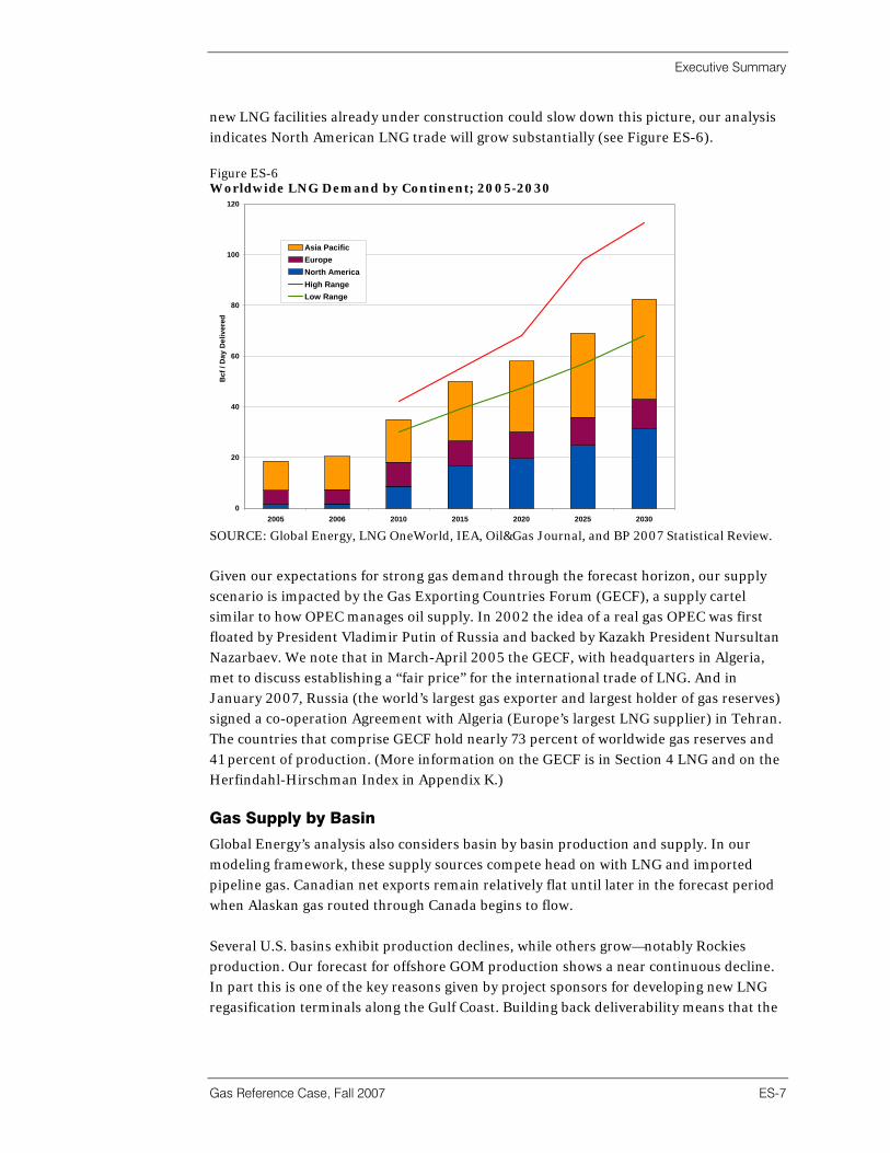
new LNG facilities already under construction could slow down this picture, our analysis indicates North American LNG trade will grow substantially (see Figure ES-6). Figure ES-6 Worldwide LNG Demand by Continent; 2005-2030
0
20
40
60
80
100
120
2005 2006 2010 2015 2020 2025 2030
Bcf
/ D
ay D
eliv
ered
Asia PacificEuropeNorth AmericaHigh RangeLow Range
SOURCE: Global Energy, LNG OneWorld, IEA, Oil&Gas Journal, and BP 2007 Statistical Review.
Given our expectations for strong gas demand through the forecast horizon, our supply scenario is impacted by the Gas Exporting Countries Forum (GECF), a supply cartel similar to how OPEC manages oil supply. In 2002 the idea of a real gas OPEC was first floated by President Vladimir Putin of Russia and backed by Kazakh President Nursultan Nazarbaev. We note that in March-April 2005 the GECF, with headquarters in Algeria, met to discuss establishing a “fair price” for the international trade of LNG. And in January 2007, Russia (the world’s largest gas exporter and largest holder of gas reserves) signed a co-operation Agreement with Algeria (Europe’s largest LNG supplier) in Tehran. The countries that comprise GECF hold nearly 73 percent of worldwide gas reserves and 41 percent of production. (More information on the GECF is in Section 4 LNG and on the Herfindahl-Hirschman Index in Appendix K.) Gas Supply by Basin
Global Energy’s analysis also considers basin by basin production and supply. In our modeling framework, these supply sources compete head on with LNG and imported pipeline gas. Canadian net exports remain relatively flat until later in the forecast period when Alaskan gas routed through Canada begins to flow. Several U.S. basins exhibit production declines, while others grow—notably Rockies production. Our forecast for offshore GOM production shows a near continuous decline. In part this is one of the key reasons given by project sponsors for developing new LNG regasification terminals along the Gulf Coast. Building back deliverability means that the
Executive Summary
ES-8
existing network of offshore, onshore, and interstate pipelines will remain well utilized in the future. Since onshore and offshore GOM production represents nearly 36 percent of current domestic production, replacing part of that decline from other sources will be challenging. Furthermore, many of the offshore GOM conventional wells lie in deep water and experience exponential decline rates, some with a first-year decline equaling 50 percent of the initial production rate. Thus, offshore GOM production is relatively expensive. Demand by Sector
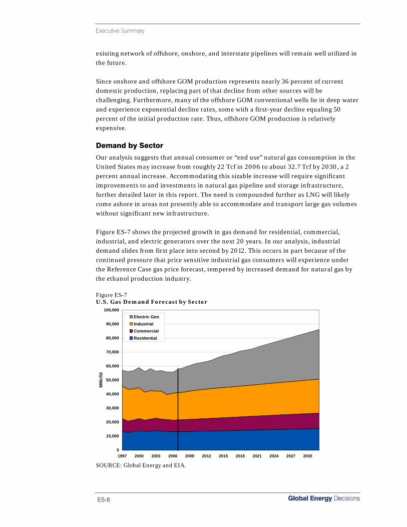
Our analysis suggests that annual consumer or “end use” natural gas consumption in the United States may increase from roughly 22 Tcf in 2006 to about 32.7 Tcf by 2030, a 2 percent annual increase. Accommodating this sizable increase will require significant improvements to and investments in natural gas pipeline and storage infrastructure, further detailed later in this report. The need is compounded further as LNG will likely come ashore in areas not presently able to accommodate and transport large gas volumes without significant new infrastructure. Figure ES-7 shows the projected growth in gas demand for residential, commercial, industrial, and electric generators over the next 20 years. In our analysis, industrial demand slides from first place into second by 2012. This occurs in part because of the continued pressure that price sensitive industrial gas consumers will experience under the Reference Case gas price forecast, tempered by increased demand for natural gas by the ethanol production industry. Figure ES-7 U.S. Gas Demand Forecast by Sector
0
10,000
20,000
30,000
40,000
50,000
60,000
70,000
80,000
90,000
100,000
1997 2000 2003 2006 2009 2012 2015 2018 2021 2024 2027 2030
MM
cf/d
Electric GenIndustrialCommercialResidential
SOURCE: Global Energy and EIA.

Executive Summary
Gas Reference Case, Fall 2007 ES-9
Continued demand growth for generation will place constant pressure on the supply industry’s ability to find and develop new sources of natural gas. In our analysis, electric generators tend to be far less price sensitive than many industrial consumers. Fuel is only one of several components to the price of delivered power so higher fuel prices will have a less than proportional impact on power prices. Much of the gas demand growth in this sector is due to the delayed impact of the electric power overbuild. Currently, many power markets are significantly overbuilt with combined cycle, gas-fired power plants. However, these plants will increasingly be used over the coming 5-10-year time frame due to continued electric load growth, retirements of older existing plants, and new environmental restrictions (e.g., NOX, SO2, CO2, Hg, etc.), which will increase the cost of generation for some solid fuel and oil-fired generators. As an example of this new paradigm where environmental factors must be taken into account, Figure ES-8 outlines the period from January 2005 through March 2007 when SO2 and NOX allowance prices were relatively very high. It indicates that the typical older vintage residual oil-fired ST was significantly penalized in relation to a gas-fired ST of similar vintage. As shown on the right-hand axis, the penalty (increased SO2/NOx adder in SIP call states and just SO2 in other states) during this period varied between $0.30/dth and nearly $1.00/dth, a hefty amount. The increased penalty for burning residual fuel oil during 2006 (not just 1 percent sulfur but for other qualities such as 0.3 percent, 0.5 percent, 0.7 percent and 2 percent as well) was one of the reasons for greatly increased natural gas usage for electric generation that year, taking over the #2 spot from nuclear power. In the future, it is anticipated that CO2 adders will similarly impact coal and well as oil plants, being at a proportional disadvantage as compared to natural gas units. Figure ES-8 SO2 and NOX Allowance Prices with Increased Adder for 1 percent Sulfur Residual Oil
$0
$500
$1,000
$1,500
$2,000
$2,500
$3,000
$3,500
Jan-
05
Feb-
05
Mar
-05
Apr
-05
May
-05
Jun-
05
Jul-0
5
Aug
-05
Sep-
05
Oct
-05
Nov
-05
Dec
-05
Jan-
06
Feb-
06
Mar
-06
Apr
-06
May
-06
Jun-
06
Jul-0
6
Aug
-06
Sep-
06
Oct
-06
Nov
-06
Dec
-06
Jan-
07
Feb-
07
Mar
-07
$ Pe
r Allo
wan
ce
$0.00
$0.10
$0.20
$0.30
$0.40
$0.50
$0.60
$0.70
$0.80
$0.90
$1.00
$ Pe
r MM
Btu
Allo
wan
ce P
enal
tyAll Resid Penalty due to NOx
Resid 1% S Penalty due to SO2
NOx Allowances (left axis)
SO2 Allowances (left axis)
SOURCE: Global Energy and Cantor-Fitzgerald Brokerage L.P.

Table of Contents
Gas Reference Case, Fall 2007 i
Executive Summary ES-1
1 Introduction And Current Market Overview 1-1
Report Objectives .....................................................................................................1-1 Market Overview .......................................................................................................1-2 Changing U.S. Gas Demand....................................................................................1-4 The Changing Role Of LNG In North America ........................................................1-5 Greater FERC And CFTC Oversight Of Gas Markets ..............................................1-7 Land Access Restrictions For Drilling ......................................................................1-9 Rising Finding & Developing (F&D) Costs And Growth ........................................1-10 Gas-Fired Generation Demand Growth .................................................................1-11 Natural Gas And Crude Oil Price Relationship ......................................................1-12 Additional Market Forces........................................................................................1-14 Report Outline.........................................................................................................1-15
2 Demand 2-1
Introduction...............................................................................................................2-1 U.S. Demand Trends ................................................................................................2-1 Ethanol ......................................................................................................................2-2 Electric Generation ...................................................................................................2-4 Canadian Demand Trends .......................................................................................2-7 Oil Sands ..................................................................................................................2-8 South Atlantic Division ..............................................................................................2-9
• Core Demand...................................................................................................2-10
• Industrial Demand............................................................................................2-10
• Electric Generation Demand ...........................................................................2-11
Middle Atlantic Division...........................................................................................2-11
• Core Demand...................................................................................................2-12
• Industrial Demand............................................................................................2-12
• Electric Generation Demand ...........................................................................2-12
New England Division.............................................................................................2-13
• Core Demand...................................................................................................2-14
• Industrial Demand............................................................................................2-14
• Electric Generation Demand ...........................................................................2-14
East North Central Division.....................................................................................2-14
• Core Demand...................................................................................................2-15
• Industrial Demand............................................................................................2-15
• Electric Generation Demand ...........................................................................2-15
West North Central Division....................................................................................2-16
• Core Demand...................................................................................................2-16

Table of Contents
ii
• Industrial Demand............................................................................................2-17
• Electric Generation Demand ...........................................................................2-17
East South Central Division ....................................................................................2-17
• Core Demand...................................................................................................2-18
• Industrial Demand............................................................................................2-18
• Electric Generation Demand ...........................................................................2-19
West South Central Division ...................................................................................2-19
• Core Demand...................................................................................................2-20
• Industrial Demand............................................................................................2-20
• Electric Generation Demand ...........................................................................2-20
Mountain Division ...................................................................................................2-20
• Core Demand...................................................................................................2-21
• Industrial Demand............................................................................................2-21
• Electric Generation Demand ...........................................................................2-22
Pacific Division........................................................................................................2-22
• Core Demand...................................................................................................2-22
• Industrial Demand............................................................................................2-23
• Electric Generation Demand ...........................................................................2-23
Conclusions ............................................................................................................2-23
3 Supply 3-1
Introduction...............................................................................................................3-1 Supply Methodology.................................................................................................3-7 Supply Cost Curves ..................................................................................................3-8 North American Supply Picture ................................................................................3-9 Working Gas Storage .............................................................................................3-17 Market Hubs ...........................................................................................................3-18 LNG Supply.............................................................................................................3-21 Supply Uncertainty..................................................................................................3-23
4 Liquefied Natural Gas (LNG) 4-1
Introduction...............................................................................................................4-1 Global Natural Gas Resources.................................................................................4-3 Liquefied Natural Gas Supply Chain .......................................................................4-5
• LNG Liquefaction ...............................................................................................4-6
• LNG Transportation ...........................................................................................4-6
• LNG Regasification ............................................................................................4-7
• LNG Storage ......................................................................................................4-7
LNG Supply Chain Economics.................................................................................4-7 Global Liquefaction Trade ........................................................................................4-8
Table of Contents
Gas Reference Case, Fall 2007 iii
• Exporting Countries ...........................................................................................4-8
• Importing Countries ...........................................................................................4-9
Global Liquefaction Projections .............................................................................4-10
• Global LNG Supply ..........................................................................................4-10
Global LNG Demand ..............................................................................................4-11 LNG Shipping Fleet ................................................................................................4-14 Overview Of LNG In North America........................................................................4-15 Outlook For Regasification in North America.........................................................4-16 Modeled North American LNG Production Through 2025.....................................4-19
• LNG Concerns .................................................................................................4-21
• LNG Siting and Permitting ...............................................................................4-23
Regasification Economics In North America..........................................................4-24 Implied Infrastructure Requirements ......................................................................4-25 Possible LNG Cartel ...............................................................................................4-26 Costs.......................................................................................................................4-28 Summary And Conclusions....................................................................................4-29
5 Infrastructure 5-1
Introduction...............................................................................................................5-1 Demand Influences...................................................................................................5-1
• Sector Demand..................................................................................................5-2
• Regional Demand ..............................................................................................5-5
Supply Influences .....................................................................................................5-7
• Lower 48 Supply Development..........................................................................5-7
• Arctic Gas...........................................................................................................5-9
• Imported Natural Gas and LNG ......................................................................5-13
• Reference Case Forecast Flows of Gas to Census Divisions ........................5-14
U.S. Natural Gas Transportation Infrastructure......................................................5-18
• National Transportation Growth and Associated Costs..................................5-26
• Regional Transportation Growth......................................................................5-26
• Natural Gas Storage Infrastructure in the United States.................................5-27
• Regional Storage Capacity..............................................................................5-30
Summary and Conclusions ....................................................................................5-32
6 Market Prices 6-1
Historical Market Perspective ...................................................................................6-1 Gas Market Evolution ...............................................................................................6-4 Natural Gas Market Phases......................................................................................6-5
• 1990s Supply Bubble.........................................................................................6-5
• Transforming Market: 2000-2004 ......................................................................6-6

Table of Contents
iv
• Market Scarcity: 2005-2008...............................................................................6-7
• LNG Renaissance: 2009-2015 ..........................................................................6-8
• Arctic Gas Flows: 2015-2025.............................................................................6-9
• Rising Costs and Depletion: 2009-2030..........................................................6-10
• Global Gas Market Integration: 2009 and Beyond..........................................6-10
Key North American Market Prices ........................................................................6-12 Seasonality Patterns ...............................................................................................6-14 Market Price Scenarios...........................................................................................6-15
• Stochastic Volatility Forecast...........................................................................6-15
7 Methodology 7-1
Introduction...............................................................................................................7-1 Base Loaded Capacity .............................................................................................7-3 Data Sources ............................................................................................................7-4 Supply .......................................................................................................................7-5 Pipeline And Storage ................................................................................................7-5 Demand ....................................................................................................................7-5 GPCM™ Overview ....................................................................................................7-6
Appendix A Annual Reference Case Price Forecast
Appendix B Henry Hub Stochastic Price Forecast
Appendix C U.S. Supply And Disposition
Appendix D Demand Forecast (MMcf/d)
Appendix E Corridor Flow Forecast
Appendix F U.S. Dry Gas Production Forecast
Appendix G WTI Oil
Appendix H WTI Reference Case Price Forecast
Appendix I History And Evolution Of Natural Gas Deregulation
Appendix J Legislative Initiatives On Carbon Trading
Appendix K Herfindahl-Hirschman Index
List of Tables
Gas Reference Case, Fall 2007 v
2-1 U.S. Gas Demand; Bcf, 2000-2030..........................................................................2-6
3-1 Domestic Gas Production (Tcf) ................................................................................3-3 3-2 Technically Recoverable Unconventional Gas Reserves ........................................3-4 3-3 U.S. Gas Supply Balance; Bcf, 2000-2030 ............................................................3-11 3-4 North American Gas Market Hubs .........................................................................3-19 3-5 North American LNG Supply through 2030; MMcf/day .........................................3-22
4-1 LNG Supply Chain Capital Cost (in $2007/Tonne LNG Capacity) ..........................4-7 4-2 Regasified LNG Supply Cost Range to the U.S. (in $2007/MMBtu)........................4-8 4-3 LNG Exporting Countries (2006) ..............................................................................4-9 4-4 LNG Importing Countries (2006) ............................................................................4-12 4-5 Approved North American Regasification Project Details .....................................4-18 4-6 Modeled Regasification Terminal Delivery through 2025 (Annual Average MMcf/d
and Utilization Rate)................................................................................................4-20 4-7 North American LNG Delivered Costs (In $2007) ..................................................4-25
5-1 Recent Pipeline Proposals......................................................................................5-20 5-2 Recent Certificated Storage Projects .....................................................................5-30 5-3 Pending Storage Projects.......................................................................................5-32
A-1 Reference Case Price Forecast (2007 $/MMBtu) ................................................... A-1
B-1 Henry Hub Stochastic Price Forecast (2007 $/MMBtu).......................................... B-1
C-1 U.S. Supply and Disposition.................................................................................... C-1
D-1 Demand Forecast ................................................................................................... D-1
E-1 Corridor Flow Forecast (MMcf/d) 2007 ................................................................... E-1
F-1 U.S. Dry Gas Production Forecast (MMcf/d) ...........................................................F-1
G-1 West Texas Intermediate Oil Prices.........................................................................G-1 G-2 Current OPEC Supply Quota...................................................................................G-2
H-1 West Texas Intermediate Reference Case Price Forecast, Supply Cost and Price Ratio ........................................................................................................ H-1

vi

List of Figures
Gas Reference Case, Fall 2007 vii
ES-1 Gulf of Mexico Monthly Natural Gas Production and Wellhead Price .................. ES-1 ES-2 Monthly LNG Imports by Country, January 1997 through July 2007.................... ES-3 ES-3 Historical Henry Hub Gas Prices........................................................................... ES-4 ES-4 Generalized Equilibrium Solution Example ......................................................... ES-5 ES-5 Source of Gas Consumed in the United States.................................................... ES-6 ES-6 Worldwide LNG Demand by Continent; 2005-2030 ............................................. ES-7 ES-7 U.S. Gas Demand Forecast by Sector.................................................................. ES-8
ES-8 SO2 and NOx, Allowance Price with Increased Adder for 1 Percent Sulfur Residual Oil ................................................................................................. ES-9
1-1 Historical Henry Hub Gas Prices, Volatility and Trend Line; October 1993-May 2007...........................................................................................1-3 1-2 U.S. Natural Gas Consumption by End User...........................................................1-4 1-3 U.S. Industrial Gas Demand Destruction .................................................................1-5 1-4 Historical U.S. Net Gas Imports ...............................................................................1-6 1-5 Proposed LNG Regasification Capacity for North America.....................................1-6 1-6 Operating and Proposed Global LNG Liquefaction Capacity .................................1-7 1-7 Prominent Trading Losses in Various Commodities................................................1-8 1-8 U.S., Canadian and Mexican Natural Gas Reserves (1982-2006) ........................1-10 1-9 U.S. Power Plant Capacity by Installation Year......................................................1-11 1-10 Electric Generation Gas Fuel Demand Growth......................................................1-12 1-11 Historic Crude Oil and Natural Gas Price Ratios (Three-Month Rolling Averages)....................................................................................................1-13 1-12 Forecast of Crude Oil-to-Natural Gas Price Ratios (Annual) .................................1-14
2-1 U.S. Gas Demand Forecast by Sector.....................................................................2-2 2-2 Historic U.S. Gasoline and Motor Fuels Consumption............................................2-3 2-3 Projected U.S. Gasoline and Motor Fuels Consumption.........................................2-3 2-4 Projected U.S. Gas Demand in Ethanol Production ................................................2-4 2-5 U.S. Gas-Fired Generation Additions and Peak Gas Consumption .......................2-5 2-6 Monthly Gas Demand; 2001-2030 ...........................................................................2-7 2-7 Canadian Gas Demand Forecast by Sector............................................................2-8 2-8 Projected Canadian Gas Demand in Oil Sand Crude Production ..........................2-9 2-9 Outlook for Demand in the South Atlantic Census Division ..................................2-10 2-10 Outlook for Demand in the Middle Atlantic Census Division .................................2-12 2-11 Outlook for Demand in the New England Census Division ...................................2-13 2-12 Outlook for Demand in the East North Central Census Division ...........................2-15 2-13 Outlook for Demand in the West North Central Census Division ..........................2-16 2-14 Outlook for Demand in the East South Central Census Division...........................2-18 2-15 Outlook for Demand in the West South Central Census Division..........................2-19 2-16 Outlook for Demand in the Mountain Census Division..........................................2-21 2-17 Outlook for Demand in the Pacific Census Division ..............................................2-22

List of Figures
viii
3-1 Correlation of Working Rigs to Gas Prices...............................................................3-1 3-2 U.S. Gulf of Mexico Gas Production and Working Gas Rigs...................................3-2 3-3 Location of Unconventional Gas Reserves in the United States .............................3-4 3-4 Unconventional Gas Production: Volume and Share of Domestic Production.................................................................................................................3-6 3-5 Representative Gas Supply Cost Curve...................................................................3-8 3-6 Changing Source of U.S. Gas Supply....................................................................3-12 3-7 U.S. Production Forecast and Trends....................................................................3-13 3-8 Long-Term Decline in U.S. Gulf of Mexico Gas Production ..................................3-14 3-9 U.S. Gulf of Mexico Working Rigs ..........................................................................3-15 3-10 U.S. Gulf of Mexico Gas Production by Depth; Percentage of Gas Production >200 m ........................................................................................3-16 3-11 U.S. Coal Bed Methane Production; As Percentage of Gulf of Mexico Production ......................................................................................3-16 3-12 U.S. Annual Storage Activity for Year 2006 through September 1, 2007 ..............3-17 3-13 North American LNG Imports .................................................................................3-21
4-1 U.S. Supply Allocation in 2006 .................................................................................4-1 4-2 Proven Natural Gas Reserves by Continent.............................................................4-3 4-3 Proven Natural Gas Reserves by Country; Percentage...........................................4-4 4-4 Proven Natural Gas Reserves by Top Countries; Tcf ..............................................4-5 4-5 Gas Reserves/Production Ratio ...............................................................................4-5 4-6 LNG Importing Countries; 1990-2006 ....................................................................4-10 4-7 Global Liquefaction Capacity (Million Tonnes/Year) ..............................................4-11 4-8 Worldwide LNG Demand Range; 2005-2030 ........................................................4-13 4-9 Worldwide LNG Demand by Continent; 2005-2030 ..............................................4-14 4-10 Global LNG Fleet through 2012 .............................................................................4-15 4-11 Existing, Under Construction and Proposed Regasification Capacity ..................4-17 4-12 Cumulative Existing, Under Construction and Proposed
Regasification Capacity..........................................................................................4-17 4-13 Cumulative Exisiting, Under Construction and Permitted
Regasification Capacity..........................................................................................4-18 4-14 North American Regasification Capacity, Production and
Utilization Percentage.............................................................................................4-21 4-15 FERC Regasification Facility Review Process........................................................4-23
5-1 Major Consumer Share (MMcf/d and Percent of Total)...........................................5-2 5-2 Demand Seasonality; 2001 (MMcf/d).......................................................................5-4 5-3 Demand Seasonality; 2030 (MMcf/d).......................................................................5-4 5-4 U.S. Census Regions and Divisions.........................................................................5-5 5-5 Major Consumer Share.............................................................................................5-6 5-6 East North Central Gas Corridor Flows MMcf/d ....................................................5-14 5-7 East South Central Gas Corridor Flows MMcf/d....................................................5-15 5-8 Middle Atlantic Gas Corridor Flows MMcf/d ..........................................................5-15
List of Figures
Gas Reference Case, Fall 2007 ix
5-9 Mountain Gas Corridor Flows MMcf/d ...................................................................5-16 5-10 New England Gas Corridor Flows MMcf/d ............................................................5-16 5-11 Pacific Gas Corridor Flows MMcf/d .......................................................................5-17 5-12 South Atlantic Gas Corridor Flows MMcf/d............................................................5-17 5-13 West North Central Gas Corridor Flows MMcf/d ...................................................5-18 5-14 West South Central Gas Corridor Flows MMcf/d...................................................5-18 5-15 Natural Gas Infrastructure in North America ..........................................................5-19 5-16 U.S. Underground Storage Capacity by Type of Reservoir ...................................5-28 5-17 Regional Working Natural Gas Storage Activity; December 1993 to Present .......5-30
6-1 Henry Hub Market Prices..........................................................................................6-1 6-2 Historical Natural Gas Price Volatility and Trend Line,
October 1993-May 2007...........................................................................................6-2 6-3 Net Annual Canadian and Mexican Imports ............................................................6-3 6-4 Historical Henry Hub and Forecast Reference Case Prices....................................6-5 6-5 Gulf of Mexico (GOM) Working Gas Rigs and Wellhead Price (Monthly Averages)...................................................................................................6-7 6-6 U.S. Gas Supply Breakdown..................................................................................6-11 6-7 Reference Case Supply Hub Prices.......................................................................6-13 6-8 Reference Case Demand Hub Prices ....................................................................6-14 6-9 Monthly Hub Prices.................................................................................................6-15 6-10 Confidence Interval for Henry Hub Market Prices (Annual) ...................................6-16 6-11 Confidence Interval for Henry Hub Market Prices (Monthly)..................................6-17
7-1 Generalized Equilibrium Solution Example ..............................................................7-1 7-2 Modeling Framework Inputs and Outputs ...............................................................7-4
7-3 Market Crossing Point ..............................................................................................7-7
G-1 Relationship between Excess Productive Capacity and Market Price ...................G-3 G-2 OPEC Production; 1st Quarter 2006 through 2nd Quarter 2007...............................G-4 G-3 World Oil Demand by Major Region; 1966-2006 ....................................................G-4 G-4 World Oil Production by Major Region; 1966-2006 ................................................G-5 G-5 Oil Production/Demand (P/D) Ratio by Region; 1996-2006 ...................................G-5 G-6 Oil Reserves/Production (R/P) Ratio by Region; 1986-2006 ..................................G-6 G-7 Reference Case Oil to Gas Price Ratio ...................................................................G-6 G-8 Confidence Interval for WTI Crude Oil Price Forecast ............................................G-7
J-1 Existing Non-Attainment Areas and Regional Cap-and-Trade Programs for NOX: .................................................................................................... J-2
J-2 Clean Air Interstate Rule (CAIR) Geographical Scope and Reduction Targets ...... J-2 J-3 States/Provinces with CO2 Initiatives in Process ..................................................... J-5
J-4 Coal Generation as a Percentage of Total Regional Generation ............................ J-6 J-5 Representative Environmental Adders to Electric Dispatch Cost (Under Specific Pricing Assumptions for NOx, SO2, and CO2) .......................... J-10


Section 1 | Introduction And Current Market Overview


Introduction And Current Market Overview
Gas Reference Case, Fall 2007 1-1
Report Objectives Global Energy’s Natural Gas Reference Case provides a comprehensive review of important natural gas market drivers and a forecast of projected gas market conditions. As of 2007, the natural gas market has entered its seventh year of unprecedented high prices, along with wide price swings. The last few years have caused many industry observers to rethink their conventional wisdom about current and future natural gas markets. Global Energy’s own analysis is no different in this regard. Others have assumed that futures prices are the best that one can do in forming market opinion and have therefore largely abandoned some aspects of fundamental research. Global Energy believes this is a risky approach to take for several reasons—not the least of which is the lack of trading liquidity beyond 18 months in the NYMEX natural gas futures market. This report’s objective is to provide an expected case analysis of current and future natural gas market conditions and drivers. Global Energy’s “down the middle” independent analysis is highly regarded in the industry and can serve as a solid base for alternative forecasts using alternative assumptions. To prepare the forecasts, Global Energy undertook a fundamental analysis of gas market supply and demand and price scenarios of the future. For this task we combine an integrated approach to energy modeling that considers competitive fuel economics, continental electric power, and coal markets along with RBAC’s GPCM natural gas market modeling platform.1 The forecasts presented for market prices for all cases are prepared to 2032. However, due to the inherent high degree of uncertainty in gas supply and demand and the current model configuration, including computer run time for LP optimization, we report the quantitative supply and demand values to 2027 only. Beyond 2027, Global Energy chose to produce an extrapolated forecast. Gas (and oil) market forecasting tends to be inherently more uncertain than other energy commodities such as power price forecasting, due to its inherent uncertainty about reserves and supply costs. In fact, most petroleum supply models are based on extrapolated statistical reserve pool plays based on highly incomplete information. In addition, the ultimate extraction cost and the role technology plays in reducing those costs are highly uncertain. No one knows with a high degree of accuracy exactly how much extractable gas resources will be available in the future and at what cost. Furthermore, the history of the petroleum extraction is punctuated with periods of intense technological innovation where new methodologies and processes have revolutionized finding, developing, and extraction methods. Some of these include 3 and 4D-seismic and micro-seismology, which have greatly improved seismic imaging and reduced dry holes; logging while drilling, which has improved operator target accuracy;
1 GPCM originally stood for Gas Pipeline Competition Model, but has been expanded to account for the entire natural gas industry.

Introduction And Current Market Overview
1-2
horizontal drilling used to produce petroleum where economic recovery was not possible with conventional methods; coil tube drill pipe, which reduces the cost to drill certain formations; deep offshore drilling and production platforms, which have extended the range of drillers and increased the area of “land” available for exploration; and finally, greatly improved computer imaging and seismic processes which enable geologists and geophysicists to better understand pools. But technological innovation tends to be lumpy in its introduction and difficult to accurately predict more than a few years forward. The introduction and innovation of each of the aforementioned technologies has greatly contributed to improving the success rate of drillers, increased the deliverability of pools, optimized the total reserves to be produced, and reduced the finding and developing costs per Mcf of natural gas. Until recently, the combination of these innovations has kept pace with the naturally decreasing gas reserve quality in many North American gas basins. At the same time, rapid expansion of the upstream industry along with rising materials costs, have created a bonanza for drillers, seismic crews, and land bonus sales, raising day rates and costs for all. The current manic pace has greatly inflated industry finding and developing costs, at least temporarily. Given all the uncertainties combined with demand uncertainty, Global Energy has also chosen to produce a stochastic volatility forecast based on Reference Case price results, historical volatility, and correlation with other market drivers. These results are presented in Section 6.
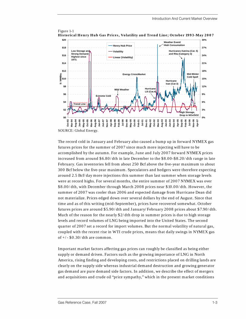
Market Overview Since Order 636 in 1993, which opened up the interstate gas price network and eliminated the merchant role enjoyed by pipeline companies, gas prices have, for the most part, remained in the $2.00 to $3.00/MMBtu range until late 2000. Figure 1-1 starts in January 1993, about half way through the infamous “gas bubble” years and includes the period post-1992 when FERC Order 636 (also known as “The Final Rule”) was put into effect making open-access mandatory in the interstate pipeline system (along with other changes in the gas industry). Henry Hub prices are shown along with 90-day rolling averages of daily volatilities on the right-side axis (calculated as a percentage per day for one standard deviation). It illustrates the historical record (including wild swings) of gas prices traded at the Henry Hub in Louisiana, North America’s main natural gas trading hub and delivery point of the NYMEX futures market. The figure shows that market prices have always been volatile, driven primarily by unexpected weather events, such as extreme cold (or warm) winters and Hurricanes Katrina and Rita in 2005. Also, there are more recent events like the price drop in 2006 due to high storage inventories and high emissions allowance prices, the mid-winter 2007 cold spell pushing Henry Hub prices into the $8-$10/MMBtu range, and the late-summer 2007 price collapse following many months of record LNG imports and high storage inventories.
Introduction And Current Market Overview
Gas Reference Case, Fall 2007 1-3
Figure 1-1 Historical Henry Hub Gas Prices, Volatility and Trend Line; October 1993-May 2007
$0
$2
$4
$6
$8
$10
$12
$14
$16
$18
$20
Oct
-93
Mar
-94
Aug
-94
Jan-
95M
ay-9
5O
ct-9
5M
ar-9
6A
ug-9
6Ja
n-97
Jun-
97N
ov-9
7A
pr-9
8Se
p-98
Feb-
99Ju
l-99
Dec
-99
May
-00
Oct
-00
Feb-
01Ju
l-01
Dec
-01
May
-02
Oct
-02
Mar
-03
Aug
-03
Jan-
04Ju
n-04
Nov
-04
Apr
-05
Sep-
05Fe
b-06
Jul-0
6N
ov-0
6A
pr-0
7
$ / M
MB
tu
0%
3%
6%
9%
12%
15%
18%
21%
24%
27%
30%
Henry Hub Price
Volatility
Linear (Volatility)
Trend Line
Weather Event/High Consumption
Energy Crisis/Market M i l i
Mild Weather
Hurricanes Katrina (Cat. 5) and Rita (Category 3)
Mid-WinterCold Spell
Hurricane Lili (Cat.4)
Hurricane Ivan (Cat 3)
Extreme Cold
Low Storage and Strong Demand;Highest since 1973.
High Storage,Drop in NOx/SO2
SOURCE: Global Energy.
The record cold in January and February also caused a bump up in forward NYMEX gas futures prices for the summer of 2007 since much more injecting will have to be accomplished by the autumn. For example, June and July 2007 forward NYMEX prices increased from around $6.80/dth in late December to the $8.00-$8.20/dth range in late February. Gas inventories fell from about 250 Bcf above the five-year maximum to about 300 Bcf below the five-year maximum. Speculators and hedgers were therefore expecting around 2.5 Bcf/day more injections this summer than last summer when storage levels were at record highs. For several months, the entire summer of 2007 NYMEX was over $8.00/dth, with December through March 2008 prices near $10.00/dth. However, the summer of 2007 was cooler than 2006 and expected damage from Hurricane Dean did not materialize. Prices edged down over several dollars by the end of August. Since that time and as of this writing (mid-September), prices have recovered somewhat. October futures prices are around $5.90/dth and January/February 2008 prices about $7.90/dth. Much of the reason for the nearly $2/dth drop in summer prices is due to high storage levels and record volumes of LNG being imported into the United States. The second quarter of 2007 set a record for import volumes. But the normal volatility of natural gas, coupled with the recent rise in WTI crude prices, means that daily swings in NYMEX gas of +/- $0.30/dth are common. Important market factors affecting gas prices can roughly be classified as being either supply or demand driven. Factors such as the growing importance of LNG in North America, rising finding and developing costs, and restrictions placed on drilling lands are clearly on the supply side whereas industrial demand destruction and growing generator gas demand are pure demand side factors. In addition, we describe the effect of mergers and acquisitions and crude oil “price sympathy,” which in the present market conditions
Introduction And Current Market Overview
1-4
where a risk premium of as much as $10-25/ barrel is “built into the price” has permitted natural gas to trade at higher prices. In the following sections Global Energy discusses several pivotal market factors that drive the natural gas market throughout the forecast horizon.
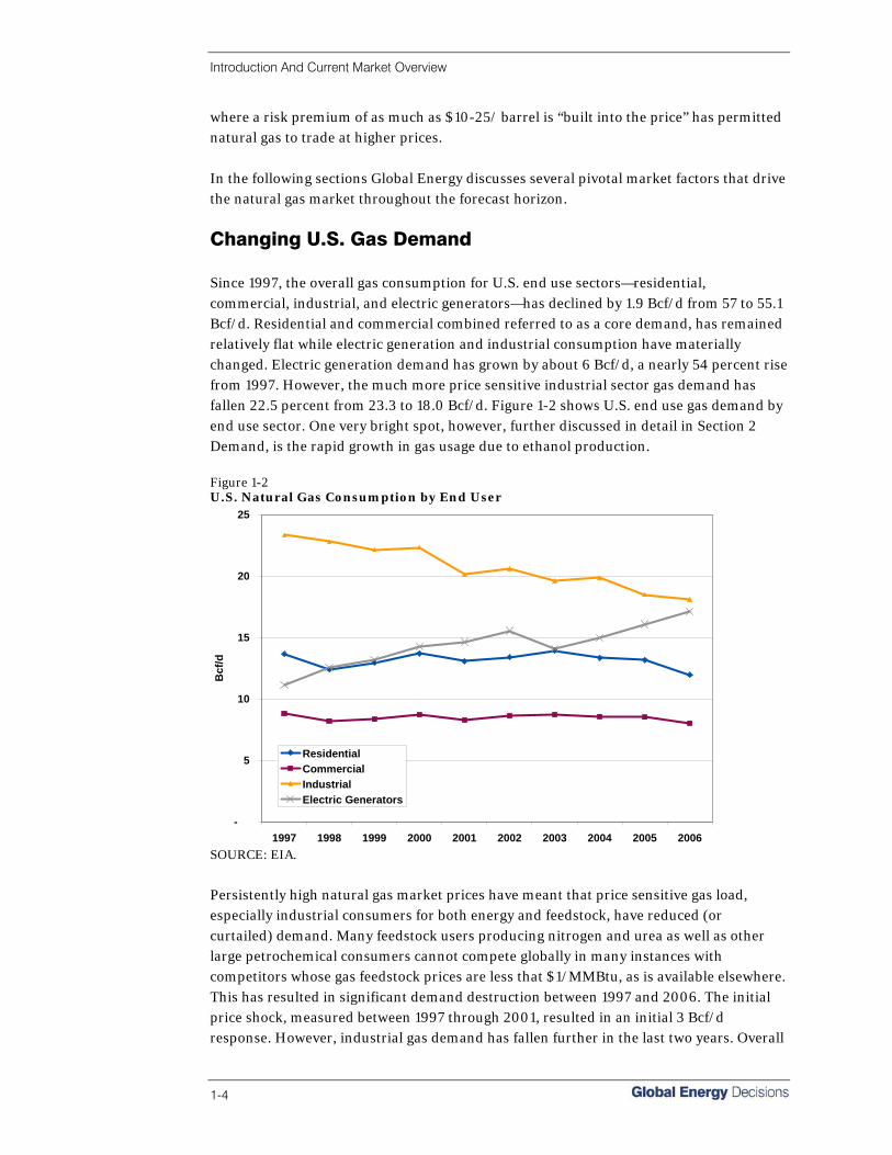
Changing U.S. Gas Demand Since 1997, the overall gas consumption for U.S. end use sectors—residential, commercial, industrial, and electric generators—has declined by 1.9 Bcf/d from 57 to 55.1 Bcf/d. Residential and commercial combined referred to as a core demand, has remained relatively flat while electric generation and industrial consumption have materially changed. Electric generation demand has grown by about 6 Bcf/d, a nearly 54 percent rise from 1997. However, the much more price sensitive industrial sector gas demand has fallen 22.5 percent from 23.3 to 18.0 Bcf/d. Figure 1-2 shows U.S. end use gas demand by end use sector. One very bright spot, however, further discussed in detail in Section 2 Demand, is the rapid growth in gas usage due to ethanol production. Figure 1-2 U.S. Natural Gas Consumption by End User
-
5
10
15
20
25
1997 1998 1999 2000 2001 2002 2003 2004 2005 2006
Bcf
/d
ResidentialCommercialIndustrialElectric Generators
SOURCE: EIA.
Persistently high natural gas market prices have meant that price sensitive gas load, especially industrial consumers for both energy and feedstock, have reduced (or curtailed) demand. Many feedstock users producing nitrogen and urea as well as other large petrochemical consumers cannot compete globally in many instances with competitors whose gas feedstock prices are less that $1/MMBtu, as is available elsewhere. This has resulted in significant demand destruction between 1997 and 2006. The initial price shock, measured between 1997 through 2001, resulted in an initial 3 Bcf/d response. However, industrial gas demand has fallen further in the last two years. Overall

Introduction And Current Market Overview
Gas Reference Case, Fall 2007 1-5
industrial demand destruction now approaches 5.25 Bcf/d as hedges unwind and belief in the permanence of higher prices works its way through industrial users and industries move overseas. Figure 1-3 shows historical U.S. industrial gas demand destruction. Figure 1-3 U.S. Industrial Gas Demand Destruction
16
17
18
19
20
21
22
23
24
1997 1998 1999 2000 2001 2002 2003 2004 2005 2006
Bcf
/d
Over 5 Bcf/d reduction
in industrialdemand
SOURCE: Global Energy and EIA.
The Changing Role Of LNG In North America Traditionally, North American gas markets have been described as a continental gas marketplace. Extensive north-south trade between Canada and the United States—as well as growing trade between Mexico and the United States—highlights this. In particular, during the 1990s, growth in U.S. imports from Canada grew substantially. Indigenous gas production from several supply basins dominates U.S. domestic trade. This level of integration has resulted in very little need for global LNG imports—until recently. Figure 1-4 shows this trend has stalled and expected to decline with LNG making up much of the shortfall in supply in recent years. Since 1995, U.S. marine LNG imports have grown from 18 Bcf to reach their all time high of 652 Bcf in 2004. However, in 2005, LNG imports declined by 93 Bcf due in part to higher natural gas prices in Europe relative to the United States. This caused some redirection of LNG cargos originally intended for the United States. Finally, net pipeline imports increased slightly over 2004. The contribution from LNG shown in the figure was provided by four LNG onshore and one offshore regasification terminals operating at about one-third of their design rating capacity. Even the higher gas prices of 2006 only caused LNG imports to recover to 623 Bcf.

Introduction And Current Market Overview
1-6
Figure 1-4 Historic U.S. Net Gas Imports
0
500
1,000
1,500
2,000
2,500
3,000
3,500
1985 1987 1989 1991 1993 1995 1997 1999 2001 2003 2005
Bcf
/Yea
rNet LNG Imports
Net Pipeline Imports
SOURCE: Global Energy.
In light of today’s relatively high gas prices, many new LNG terminals have been proposed for the United States, Canada, and Mexico. Project developers, some of whom are integrated producers with stranded gas, see increased LNG trade serving their own corporate interests as well as their nation’s desire for an economic, clean, and uninterrupted supply of energy. Presently, there is a development boom for LNG projects as developers vie for the first mover advantage in an attempt to monetize their stranded gas reserves worldwide. Figure 1-5 shows the announced level of LNG regasification capacity in bcf/d for North America by on line year. Figure 1-5 Proposed LNG Regasification Capacity for North America
-
10,000
20,000
30,000
40,000
50,000
60,000
70,000
2007 2008 2009 2010 2011
mm
cf/d
ProposedApprovedConstructionOperational
SOURCE: Global Energy.
Introduction And Current Market Overview
Gas Reference Case, Fall 2007 1-7
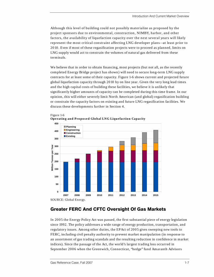
Although this level of building could not possibly materialize as proposed by the project sponsors due to environmental, construction, NIMBY, harbor, and other factors, the availability of liquefaction capacity over the next several years will likely represent the most critical constraint affecting LNG developer plans—at least prior to 2010. Even if most of these regasification projects were to proceed as planned, limits on LNG supply would act to constrain the volumes of natural gas delivered from these terminals. We believe that in order to obtain financing, most projects (but not all, as the recently completed Energy Bridge project has shown) will need to secure long-term LNG supply contracts for at least some of their capacity. Figure 1-6 shows current and projected future global liquefaction capacity through 2010 by on line year. Given the very long lead times and the high capital costs of building these facilities, we believe it is unlikely that significantly higher amounts of capacity can be completed during this time frame. In our opinion, this will either severely limit North American (and global) regasification building or constrain the capacity factors on existing and future LNG regasification facilities. We discuss these developments further in Section 4. Figure 1-6 Operating and Proposed Global LNG Liquefaction Capacity
0
50
100
150
200
250
300
350
400
450
2007 2008 2009 2010 2011 2012 2013 2014 2015
Mill
ion
Tonn
es p
er Y
ear
PlanningEngineeringConstructionExisting
SOURCE: Global Energy.
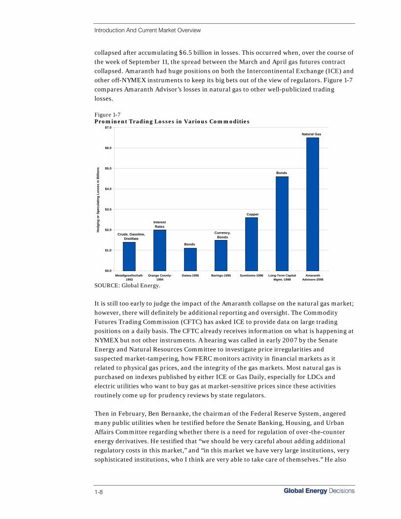
Greater FERC And CFTC Oversight Of Gas Markets In 2005 the Energy Policy Act was passed, the first substantial piece of energy legislation since 1992. The policy addresses a wide range of energy production, transportation, and regulatory issues. Among other duties, the EPAct of 2005 gives sweeping new tools to FERC, including civil penalty authority to prevent market manipulation (in response to an assortment of gas trading scandals and the resulting reduction in confidence in market indices). Since the passage of the Act, the world’s largest trading loss occurred in September 2006 when the Greenwich, Connecticut, “hedge” fund Amaranth Advisors
Introduction And Current Market Overview
1-8
collapsed after accumulating $6.5 billion in losses. This occurred when, over the course of the week of September 11, the spread between the March and April gas futures contract collapsed. Amaranth had huge positions on both the Intercontinental Exchange (ICE) and other off-NYMEX instruments to keep its big bets out of the view of regulators. Figure 1-7 compares Amaranth Advisor’s losses in natural gas to other well-publicized trading losses. Figure 1-7 Prominent Trading Losses in Various Commodities
$0.0
$1.0
$2.0
$3.0
$4.0
$5.0
$6.0
$7.0
Metallgesellschaft-1993
Orange County-1994
Daiwa-1995 Barings-1995 Sumitomo-1996 Long-Term CapitalMgmt.-1998
AmaranthAdvisors-2006
Hed
ging
or S
pecu
latin
g Lo
sses
in B
illio
ns
Natural Gas
Crude, Gasoline,Distillate
InterestRates
Bonds
Currency,Bonds
Copper
Bonds
SOURCE: Global Energy.
It is still too early to judge the impact of the Amaranth collapse on the natural gas market; however, there will definitely be additional reporting and oversight. The Commodity Futures Trading Commission (CFTC) has asked ICE to provide data on large trading positions on a daily basis. The CFTC already receives information on what is happening at NYMEX but not other instruments. A hearing was called in early 2007 by the Senate Energy and Natural Resources Committee to investigate price irregularities and suspected market-tampering, how FERC monitors activity in financial markets as it related to physical gas prices, and the integrity of the gas markets. Most natural gas is purchased on indexes published by either ICE or Gas Daily, especially for LDCs and electric utilities who want to buy gas at market-sensitive prices since these activities routinely come up for prudency reviews by state regulators. Then in February, Ben Bernanke, the chairman of the Federal Reserve System, angered many public utilities when he testified before the Senate Banking, Housing, and Urban Affairs Committee regarding whether there is a need for regulation of over-the-counter energy derivatives. He testified that “we should be very careful about adding additional regulatory costs in this market,” and “in this market we have very large institutions, very sophisticated institutions, who I think are very able to take care of themselves.” He also
Introduction And Current Market Overview
Gas Reference Case, Fall 2007 1-9
stated that “it seems unlikely that manipulation, in most cases, would come from the [over-the-counter] markets since the exchanges provide a good venue for determining prices.” Responses by many industry groups, such as the American Public Gas Association (APGA), criticized Chairman Bernanke and complained about the lack of transparency of the OTC market and the susceptibility of natural gas contracts to price volatility and price manipulation, citing that the deliverable supply of natural gas and the capacity to deliver is often small relative to the size of the derivative position held by large traders. 2 The CFTC has fined over $300 million in penalties for market abuses associated with trading in the OTC markets. The member companies comprising the APGA and the American Gas Association (AGA) have stated that Amaranth has led to a real loss of confidence in physical gas trading, as well as futures markets and that prudency reviews by state commissions may become much more rigorous. Disallowances by state commissions during Purchased Gas Cost Adjustment (PGA) hearings are a serious concern. Despite provisions in EPAct2005 to curb abuse, it appears there may still be futile attempts at market manipulation from time to time, even in such a liquid commodity as natural gas. Other stakeholders that are concerned about natural gas prices and manipulation besides the Risk Management Committees of electric and gas utilities are industrial customers, state regulatory agencies, departments of public utility control, state consumer counsels, attorneys general, and governors. In June, the CFTC proposed rules that would significantly expand recordkeeping requirements for energy traders, such as keeping records on transactions involving the same commodity in all venues, including electronic trading platforms, the cash market, over-the-counter, and other non-reporting hedging transactions. In late June, a bipartisan Senate subcommittee recommended that ICE should be brought under government regulation, concluding that Amaranth distorted the price in the natural gas futures markets through excessive speculation and at one point held 70 percent of the open interest contracts in the November 2006 NYMEX futures contract and raised the cost of gas to industry and consumers. The 532-page report concluded that the futures market is inherently unbalanced with many gas producers willing to sell futures to hedge production and fewer end-users buying contracts to hedge consumption. While Amaranth had no trouble finding sellers in the winter months when prices were high, the hedge fund was crippled by a lack of buyers at prices driven higher by the hedge fund’s own trading.
Land Access Restrictions For Drilling Land access restrictions for petroleum exploration and development activity have prominently captured public attention in recent years. Concerns over endangered species, water usage, groundwater pollution, disturbance, and other effects of industrialization in rural communities have reduced the land available for drilling that otherwise would have
2 American Public Gas Association, February 22, 2007 letter from President Bert Kalisch to Chairman of the Federal Reserve Ben Bernanke.

Introduction And Current Market Overview
1-10
been the case. The interesting factor to note is that although in many ways the industry has been encouraged to use clean burning natural gas, parallel and consistent policies aimed to increase supply have not been forthcoming. The two most often cited cases are restrictions on drilling in Alaska and in some parts of the Rocky Mountains. The EPAct of 2005 also streamlines the LNG terminal application process with the federal government. It also reaffirms the exclusive federal regulation of offshore LNG terminals. Royalty relief under very low oil and gas market price conditions is also provided for unconventional and marginal producers and where CO2 injection is used in enhanced recovery. Royalty relief for deep water drilling in over 400 meters of water depth was also enacted.
Rising Finding & Developing (F&D) Costs And Growth In the current market environment, U.S. natural gas reserves have risen back to their relatively high 1980s level. Many producers have been successfully finding and booking more reserve than they have produced each year for the last several years. Also, the increase in reserve is due to how reserves get booked on company financial statements. Natural gas reserves (but not “resources”) are those where, under current market conditions, resource development and extraction is profitable. So, as gas prices rise, all things being equal, more resources cross over into the “reserve” category. Figure 1-8 shows the trend of U.S., Canadian, and Mexican proved dry gas reserves. Figure 1-8 U.S., Canadian and Mexican Natural Gas Reserves (1982-2006)
0
50
100
150
200
250
300
350
400
1982 1984 1986 1988 1990 1992 1994 1996 1998 2000 2002 2004 2006
Res
erve
s at
end
of y
ear (
Tcf)
Mexico
Canada
United States
SOURCE: BP 2007 World Energy Report.
Increasing natural gas reserves only tell part of the market picture. Recent reserve additions have largely consisted of relatively small gas pools in tight or unconventional sands and shale, which makes extraction more difficult and therefore more expensive to
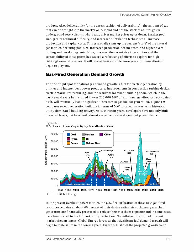
Introduction And Current Market Overview
Gas Reference Case, Fall 2007 1-11
produce. Also, deliverability (or the excess cushion of deliverability)—the amount of gas that can be brought into the market on demand and not the stock of natural gas in underground reservoirs—is what really drives market prices up or down. Smaller pool size, greater technical difficulty, and increased stimulation techniques all increase production and capital costs. This essentially sums up the current “state” of the natural gas market, declining pool size, increased production decline rates, and higher overall finding and developing costs. Note, however, the recent rise in gas prices and the sustainability of those prices has caused a refocusing of efforts to explore for high-risk/high-reward reserves. It will take at least a couple more years for these efforts to begin to play out.
Gas-Fired Generation Demand Growth The one bright spot for natural gas demand growth is fuel for electric generation by utilities and independent power producers. Improvements in combustion turbine design, electric market restructuring, and the resultant merchant building boom, which in the past several years has resulted in over 225,000 MW of additional gas-fired capacity being built, will eventually lead to significant increases in gas fuel for generation. Figure 1-9 compares recent generation building in terms of MW installed by year, with historical utility-dominated building activity. Note, in recent years, developers have not only built to record levels, but have built almost exclusively natural gas-fired power plants. Figure 1-9 U.S. Power Plant Capacity by Installation Year
SOURCE: Global Energy.
In the present overbuilt power market, the U.S. fleet utilization of these new gas-fired resources remains at about 40 percent of their design rating. As such, many merchant generators are financially pressured to reduce their merchant exposure and in some cases have been forced to file for bankruptcy protection. Notwithstanding difficult present market circumstances, Global Energy forecasts that significant fuel demand growth will begin to materialize in the coming years. Figure 1-10 shows the projected growth trend
0
10,000
20,000
30,000
40,000
50,000
60,000
70,000
1950 1955 1960 1965 1970 1975 1980 1985 1990 1995 2000 2005 2010 2015
Cap
acity
Inst
alla
tions
(MW
)
Vertically Integrated Utilities
PURPA QF Era
Rise of theMerchant
EWGs
Oil EmbargoCAA1970
EPAct2005
EPAct1992
CAA 1990
PURPA1978
RTO NOPR1999
New Coal
2nd GenerationNuclear
Coal
Hydro
Renew
Nuclear
Oil
Natural Gas
OtherCoal
Hydro
Renew
Nuclear
Oil
Natural Gas
Other

Introduction And Current Market Overview
1-12
over the next eight years. In particular, gas fuel demand derived from our new Fall 2007 Power Reference Case analysis indicates that competitive power market forces and the abundance of idle combined cycle capacity will cause significant increases in gas demand between 2006 and 2030. The average usage per day is projected to increase by 16.6 Bcf/d—a 97 percent increase over 2006. Figure 1-10 Electric Generation Gas Fuel Demand Growth
0
5
10
15
20
25
30
35
40
2000 2006 2008 2010 2015 2020 2025 2030
Bcf
/ D
ay
SOURCE: Global Energy.
Another factor affecting near-term fuel requirements in those markets with significant gas steam capacity has been the substitution away from gas steam generation and towards gas combined cycle. This is important to note since new CC plants are about 30 percent more efficient in fuel usage and have resulted in a net fuel consumption reduction in certain markets. The substitution away from gas steam plants and the observed low capacity utilization of many of the new plants has meant that very little of the presently high natural gas prices can be attributed to growth in the merchant industry. Without adequate new sources of natural gas—in particular LNG—becoming available in a timely manner, as we forecast in our Natural Gas Reference Case, consumption growth in this sector will keep pressuring prices higher. Also, due to the relatively inelastic nature of generators (at least relative to industrial gas demand), if sufficient LNG and other supply sources do not materialize as forecasted, we would then also expect to see additional displacement in industrial gas demand.
Natural Gas And Crude Oil Price Relationship Crude oil and natural gas prices often trade in sympathy with each other. This relationship is observed in both NYMEX future market prices and historically in the spot market—although the correlation is by no means perfect. Figure 1-11 shows that

Introduction And Current Market Overview
Gas Reference Case, Fall 2007 1-13
historically the ratio has actually ranged widely from as high as 17.5 to 1 down to as little as 5.8 to 1, which is the point of “energy parity” between crude oil and natural gas.3 If natural gas and crude oil were perfect substitutes for each other, this parity ratio would remain a constant. Figure 1-11 Historic Crude Oil and Natural Gas Price Ratios (Three-Month Rolling Averages)
$0
$1
$2
$3
$4
$5
$6
$7
$8
$9
$10
$11
$12
$13Ju
l-86
May
-87
Mar
-88
Jan-
89
Nov
-89
Sep-
90
Jul-9
1
May
-92
Mar
-93
Jan-
94
Nov
-94
Sep-
95
Jul-9
6
May
-97
Mar
-98
Jan-
99
Nov
-99
Sep-
00
Jul-0
1
May
-02
Mar
-03
Jan-
04
Nov
-04
Sep-
05
Jul-0
6
May
-07
$/D
th
0.0
1.5
3.0
4.5
6.0
7.5
9.0
10.5
12.0
13.5
15.0
16.5
18.0
19.5
Pric
e R
atio
(
$/bb
l. O
il to
$/d
th G
as )
Wellhead Gas
WTI Crude Oil
Oil / Gas Ratio
Oil - Gas Parity
Energy Crisis /Market Manipulation
Hurricane Katrina
Weather Event / High Demand
SOURCE: EIA and Global Energy.
However, the typical price ratio tends to be around the 8 to 1 level. The ratio moves higher as the market value of gas to oil falls and, conversely, over the last 10 years, this ratio has generally trended downward reaching parity with oil in 2001 and 2003 when gas price spikes occurred. Global Energy believes that the first half of this period saw high gas-oil ratios based on the “natural gas bubble” market. The over supply of gas was caused by a variety of market and regulatory reasons and persisted throughout North America for most of the 1990s. More recently our analysis has concluded that recent high natural gas prices, which translated to relatively low oil price to gas price ratios between 1997 and 2005, will not persist forever due mainly to unconventional, frontier, and LNG supply response. However, demand for gas as a “green” fuel in power plant applications is strong. Figure 1-12 illustrates Global Energy’s expectation that the ratio will be around 9:1, and for the price relationship to remain for the most part within the 7.5:1 to 8.5:1 1 range during the first three-fifths of the forecast years. Then the ratio gradually declines (gas becomes relatively more valuable) to around 7.2 to 1 after the MacKenzie Delta gas and Alaskan pipeline gas is absorbed by the intercontinental gas system.
3 Parity at this level exists since there are 5.8 MMBtu of natural gas per barrel of crude oil.

Introduction And Current Market Overview
1-14
Figure 1-12 Forecast of Crude Oil-to-Natural Gas Price Ratios (Annual)
0.0
1.5
3.0
4.5
6.0
7.5
9.0
10.5
12.0
13.5
15.0
2007 2009 2011 2013 2015 2017 2019 2021 2023 2025 2027 2029 2031
Rat
io ($
/bbl
) / $
/MM
Btu
)
Natural gas becoming relatively more valuable compared to crude oil
Natural gas becoming relatively less valuable compared to crude oil
Price ratio of 5.8 indicates crude oil-gas energy price parity
SOURCE: Global Energy. In this report, Global Energy presents our Reference Case oil price forecast for West Texas Intermediate oil in Appendix E, which was used as an input in the preparation of the Natural Gas Reference Case forecast.
Additional Market Forces Although this survey has been brief, we wanted to touch on many of the more important current market trends affecting natural gas markets. Other factors, such as alleged hedge fund speculation and the reluctance of energy firms to adequately re-invest their cash flow in exploration and development, have also been cited in the trade press. The former charge has recently received some public attention with the proponents of these beliefs charging that hedge funds are treating vital energy commodities like a casino. In our view there is little evidence to support this assertion. Furthermore, the counteracting trading undertaken by some individual hedge funds would be self-correcting. The bottom line is that no single entity or consortium (tacit or collusive) could hold any degree of market power in such liquid commodities. Hedge funds are attracted to liquidity markets where there is volatility to trade around. There is no doubt that the present gas and oil markets fulfill these requirements. Diminished cash flow reinvestment on the part of the majors and independents has also received attention. In past commodity cycles, rising prices have led to increased cash flow and then proportional capital investment. Although we have seen all three mentioned, the level of reinvestment has been somewhat muted and delayed on the part of many. Part of
Introduction And Current Market Overview
Gas Reference Case, Fall 2007 1-15
this is due to the major oil producers who have turned much of their focus away from North America concentrating instead on overseas investment opportunities. In other cases, firms have been improving their balance sheet, buying down debt, and repurchasing shares. However, record high profits, in light of reduced activity especially in the offshore Gulf of Mexico, have led some to call for windfall taxes to be levied.
Report Outline The remainder of the report is organized as follows: • Section 2 discusses natural gas demand. • Section 3 presents natural gas supply. • Section 4 focuses on LNG growth—both on the regasification side and upstream at
liquefaction centers. • Section 5 discusses gas transportation and storage infrastructure and investment
growth necessary to support forecast demand growth expected. • Section 6 presents the Reference Case Market price forecasts as well as estimated
confidence band forecasts. • Section 7 discusses the methodology used to prepare the analysis. Finally, annual
market prices for 36 key gas market price zones are reported in the data appendix for each scenario. Monthly price forecast results and other supplemental data are reported in a separate Excel data file.


Section 2 | Demand


Demand
Gas Reference Case, Fall 2007 2-1
Introduction This section reports the demand modeling results prepared by Global Energy. The forecast results are prepared through 2032 for residential, commercial, industrial, and electric generation sectors. Collectively these are denoted as “end use” demand. The forecast of demand is consistent with the market supply and prices presented elsewhere in the report. Global Energy also forecasts the natural gas supply sector’s own consumption of gas including on lease, pipeline, and gas processing plant fuel—although these are omitted from the analysis presented in this section. To forecast residential, commercial, and industrial gas demand Global Energy developed state-by-state econometric modeling equations.1 For electric generator gas consumption we used our own electric market Reference Case forecast of gas demand for all North America Electric Reliability Council (NERC) regions. The degree of price sensitivity (elasticity) and forecast of economic growth and population are some of the key variables used to forecast gas demand for core (residential and commercial) and industrial sectors. Results are shown for each U.S. census division and for Canada as a whole. We did not undertake a comprehensive analysis of Mexican gas demand, but did use Mexican federal demand forecast data in our modeling and analysis. At some point in the future, Global Energy expects to provide a more comprehensive demand and supply analysis of the Mexican natural gas and electric sectors. Additional methodological information is presented in Section 7 Methodology.
U.S. Demand Trends Widespread interstate natural gas trade began in earnest in the United States following World War II. Prior to that time, several regional natural gas markets had developed, but large scale interstate commerce and widespread core and industrial gas demand did not develop throughout the country until after this period. Actual natural gas demand first peaked in the late 1970s dropping off after passage of the Power Plant and Industrial Fuel Use Act (FUA) in 1978, which restricted gas use until its repeal in 1987. Then more recently in 2000, U.S. core, industrial, and electric generation demands reached 59 Bcf/d (about 21.5 Tcf). During much of the historical period and up to the present, the proportions of gas consumed among the different sectors have changed markedly. Historical and Global Energy’s forecast for U.S. end use demand are shown in Figure 2-1. Noticeably, from this figure changes in demand arising from weather-driven events (unusually cold or hot weather) mainly impact residential and commercial gas/energy demand. It is also clear that since the price spike of 2000, industrial gas demand has decreased. During the period shown industrial demand actually peaked in 1997. Since then, industrial demand has declined by 23 percent or about 5.4 Bcf/d before it reached bottom in the 2004-2005 time frame. Much of this actual “demand destruction” resulted from more price sensitive industrial load being
1 Econometric equations were developed in partnership with the Colorado School of Mines.

Demand
2-2
shed, although part of this amount was due to damage from Hurricanes Katrina and Rita. In the last few years, however, industrial demand has regained about a quarter of that loss and rebounded 1.4 Bcf/day. Nearly half of this gain is due to the increased use of natural gas in ethanol production. Figure 2-1 U.S. Gas Demand Forecast by Sector
0
10,000
20,000
30,000
40,000
50,000
60,000
70,000
80,000
90,000
100,000
1997 2002 2007 2012 2017 2022 2027 2032
MM
cf/d
Electric GenIndustrialCommercialResidential
SOURCE: Global Energy and EIA.
Ethanol Although there have been many “gas intensive” industries moving overseas in the last decade or more (e.g., steel, fertilizer, non-ferrous metals, various labor-intensive manufacturing, etc.), there is a bright spot with the highest growth of industrial gas usage. For many years, natural gas has been used in the production of ethanol, creating steam for distillation and heat for grain drying, almost exclusively corn. As MTBE (methyl tertiary-butyl ether) lost its popularity as a gasoline additive for increasing motor octane due to environmental concerns, gasoline refiners have been turning to ethanol as a substitute, blending it with gasoline to increase octane numbers. Additionally, ethanol is being used as a clean motor fuel in its own right; for example, E85 is a blend of 85 percent ethanol and 15 percent gasoline. Grain farmers dedicated more land to growing corn for ethanol, and production has sharply increased from about 1.8 billion gallons in 2001 to 4.1 billion gallons in 2006. Finally, ethanol’s use in motor fuel has increased since 2000, even as gasoline consumption increased, from 1.27 percent to 2.85 percent of total consumption, as seen in Figure 2-2. Gas used in ethanol production is expected to continue to be a growth industry, even if there is a trend to move away from corn to other feedstocks, such as switchgrass or miscanthus.
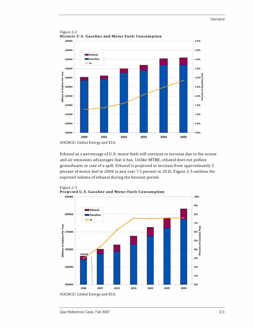
Demand
Gas Reference Case, Fall 2007 2-3
Figure 2-2 Historic U.S. Gasoline and Motor Fuels Consumption
100000
105000
110000
115000
120000
125000
130000
135000
140000
145000
150000
2000 2001 2002 2003 2004 2005
Mill
ions
of G
allo
ns P
er Y
ear
0.0%
0.5%
1.0%
1.5%
2.0%
2.5%
3.0%
3.5%
4.0%
4.5%
5.0%
Perc
ent o
f Gas
olin
e Po
ol
Ethanol
Gasoline
%
SOURCE: Global Energy and EIA.
Ethanol as a percentage of U.S. motor fuels will continue to increase due to the octane and air emissions advantages that it has. Unlike MTBE, ethanol does not pollute groundwater in case of a spill. Ethanol is projected to increase from approximately 3 percent of motor fuel in 2006 to just over 7.5 percent in 2015. Figure 2-3 outlines the expected volume of ethanol during the forecast period. Figure 2-3 Projected U.S. Gasoline and Motor Fuels Consumption
100000
125000
150000
175000
200000
225000
2006 2007 2010 2015 2020 2025 2030
Mill
ions
of G
allo
ns P
er Y
ear
0%
1%
2%
3%
4%
5%
6%
7%
8%
9%
10%Pe
rcen
t of G
asol
ine
Pool
Ethanol
Gasoline
%
Actual
SOURCE: Global Energy and EIA.
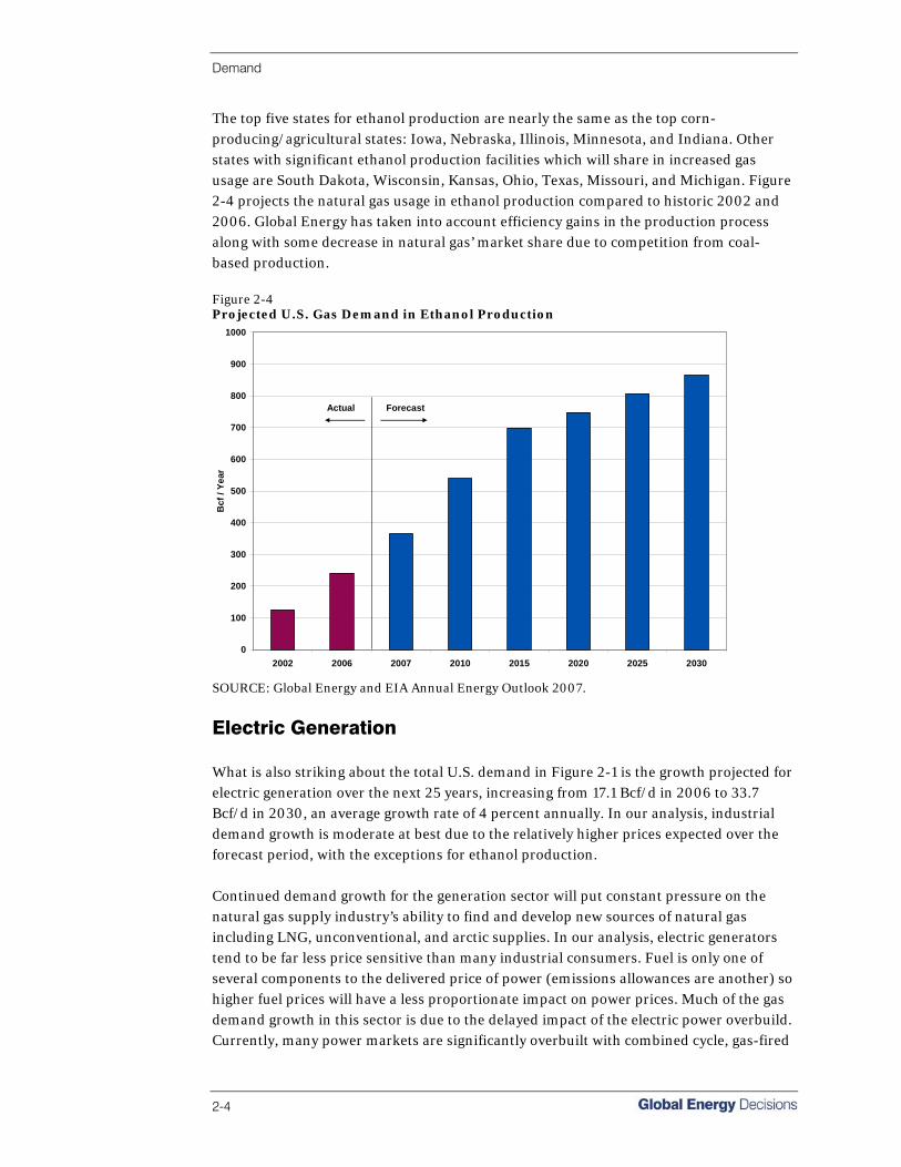
Demand
2-4
The top five states for ethanol production are nearly the same as the top corn-producing/agricultural states: Iowa, Nebraska, Illinois, Minnesota, and Indiana. Other states with significant ethanol production facilities which will share in increased gas usage are South Dakota, Wisconsin, Kansas, Ohio, Texas, Missouri, and Michigan. Figure 2-4 projects the natural gas usage in ethanol production compared to historic 2002 and 2006. Global Energy has taken into account efficiency gains in the production process along with some decrease in natural gas’ market share due to competition from coal-based production. Figure 2-4 Projected U.S. Gas Demand in Ethanol Production
0
100
200
300
400
500
600
700
800
900
1000
2002 2006 2007 2010 2015 2020 2025 2030
Bcf
/ Ye
ar
Actual Forecast
SOURCE: Global Energy and EIA Annual Energy Outlook 2007.
Electric Generation What is also striking about the total U.S. demand in Figure 2-1 is the growth projected for electric generation over the next 25 years, increasing from 17.1 Bcf/d in 2006 to 33.7 Bcf/d in 2030, an average growth rate of 4 percent annually. In our analysis, industrial demand growth is moderate at best due to the relatively higher prices expected over the forecast period, with the exceptions for ethanol production. Continued demand growth for the generation sector will put constant pressure on the natural gas supply industry’s ability to find and develop new sources of natural gas including LNG, unconventional, and arctic supplies. In our analysis, electric generators tend to be far less price sensitive than many industrial consumers. Fuel is only one of several components to the delivered price of power (emissions allowances are another) so higher fuel prices will have a less proportionate impact on power prices. Much of the gas demand growth in this sector is due to the delayed impact of the electric power overbuild. Currently, many power markets are significantly overbuilt with combined cycle, gas-fired

Demand
Gas Reference Case, Fall 2007 2-5
power plants. Figure 2-5 indicates the historic growth spurt of gas-fired generation along with the peak hourly gas load connected. Figure 2-5 U.S. Gas-Fired Generation Additions and Peak Gas Consumption
0
10,000
20,000
30,000
40,000
50,000
60,000
1999 2000 2001 2002 2003 2004 2005 2006 2007
Meg
awat
t Cap
acity
0
500
1000
1500
2000
MM
cf /
Hou
r
Combined-Cycle Combustion Turbine, Steam Turbine and IC Theoretical Connected Gas Load
SOURCE: Global Energy.
However, these plants will increasingly be used over the forecast period due to continued electric load growth, retirements of older existing plants, and new environmental restrictions, which will increase the cost of generation for some solid fuel and oil-fired generators. Our analysis also indicates that at current and forecast gas prices, new coal projects will be economic to build in many regions, but building new coal-fired plants will face many other obstacles. Global Energy’s Fall 2007 Power Market Advisory Reference Case allows for the building of economic coal plants, but only a few new projects will go into service during the next five years due to the difficulties encountered during the permitting process. Further, once fully permitted, the construction of a coal-fired plant will require four to five years to complete. Table 2-1 shows U.S. historical and projected gas demand through 2030 for the Reference Case Forecast. Also shown are supply industry consumption of fuel (pipeline, lease, and plant fuel) and gas storage.
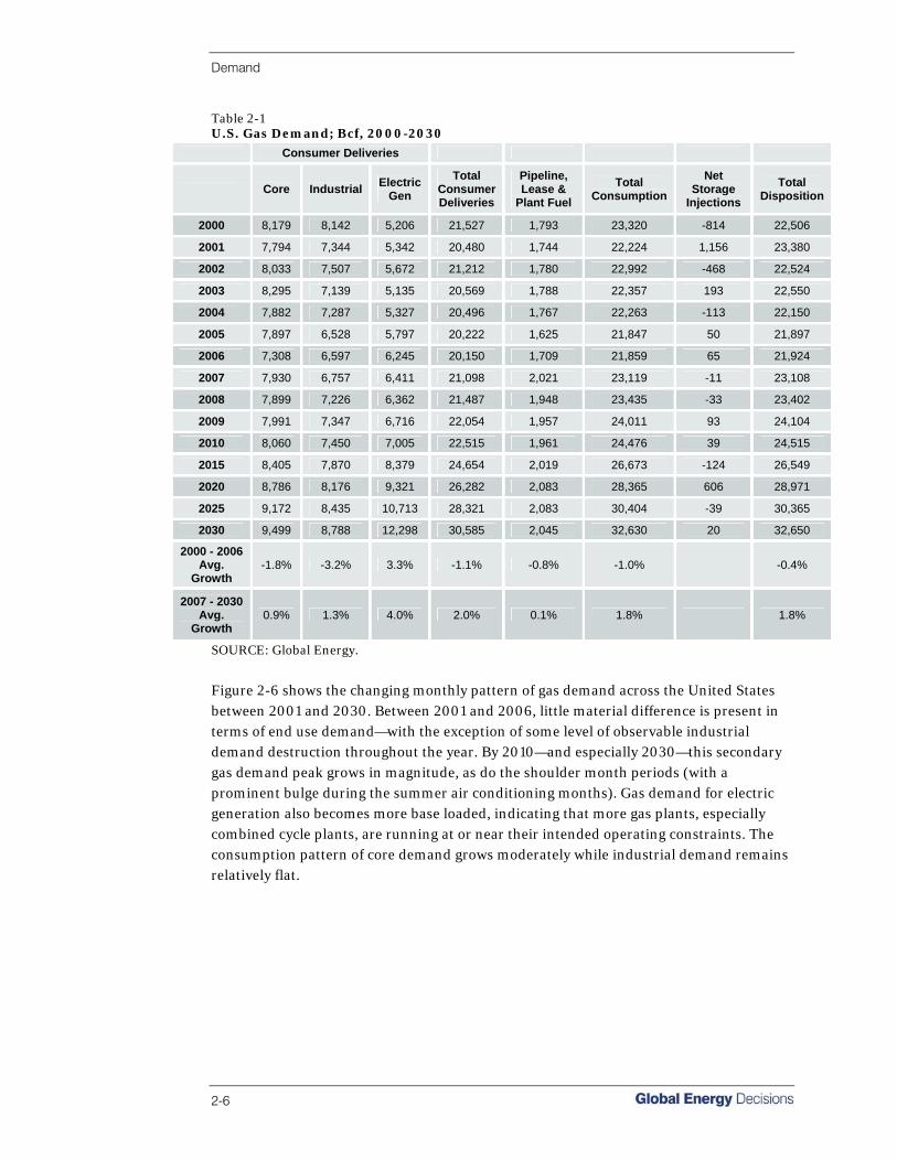
Demand
2-6
Table 2-1 U.S. Gas Demand; Bcf, 2000-2030
Consumer Deliveries
Core Industrial Electric Gen
Total Consumer Deliveries
Pipeline, Lease &
Plant Fuel Total
Consumption
Net Storage
Injections Total
Disposition
2000 8,179 8,142 5,206 21,527 1,793 23,320 -814 22,506
2001 7,794 7,344 5,342 20,480 1,744 22,224 1,156 23,380
2002 8,033 7,507 5,672 21,212 1,780 22,992 -468 22,524
2003 8,295 7,139 5,135 20,569 1,788 22,357 193 22,550
2004 7,882 7,287 5,327 20,496 1,767 22,263 -113 22,150
2005 7,897 6,528 5,797 20,222 1,625 21,847 50 21,897
2006 7,308 6,597 6,245 20,150 1,709 21,859 65 21,924
2007 7,930 6,757 6,411 21,098 2,021 23,119 -11 23,108
2008 7,899 7,226 6,362 21,487 1,948 23,435 -33 23,402
2009 7,991 7,347 6,716 22,054 1,957 24,011 93 24,104
2010 8,060 7,450 7,005 22,515 1,961 24,476 39 24,515
2015 8,405 7,870 8,379 24,654 2,019 26,673 -124 26,549
2020 8,786 8,176 9,321 26,282 2,083 28,365 606 28,971
2025 9,172 8,435 10,713 28,321 2,083 30,404 -39 30,365
2030 9,499 8,788 12,298 30,585 2,045 32,630 20 32,650
2000 - 2006 Avg.
Growth -1.8% -3.2% 3.3% -1.1% -0.8% -1.0% -0.4%
2007 - 2030 Avg.
Growth 0.9% 1.3% 4.0% 2.0% 0.1% 1.8% 1.8%
SOURCE: Global Energy.
Figure 2-6 shows the changing monthly pattern of gas demand across the United States between 2001 and 2030. Between 2001 and 2006, little material difference is present in terms of end use demand—with the exception of some level of observable industrial demand destruction throughout the year. By 2010—and especially 2030—this secondary gas demand peak grows in magnitude, as do the shoulder month periods (with a prominent bulge during the summer air conditioning months). Gas demand for electric generation also becomes more base loaded, indicating that more gas plants, especially combined cycle plants, are running at or near their intended operating constraints. The consumption pattern of core demand grows moderately while industrial demand remains relatively flat.
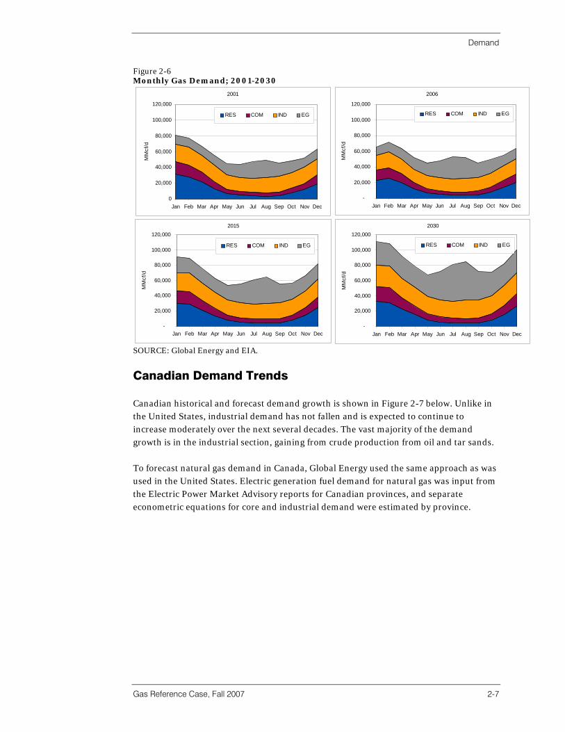
Demand
Gas Reference Case, Fall 2007 2-7
Figure 2-6 Monthly Gas Demand; 2001-2030
2001
0
20,000
40,000
60,000
80,000
100,000
120,000
Jan Feb Mar Apr May Jun Jul Aug Sep Oct Nov Dec
MM
cf/d
RES COM IND EG
2015
-
20,000
40,000
60,000
80,000
100,000
120,000
Jan Feb Mar Apr May Jun Jul Aug Sep Oct Nov Dec
MM
cf/d
RES COM IND EG
2006
-
20,000
40,000
60,000
80,000
100,000
120,000
Jan Feb Mar Apr May Jun Jul Aug Sep Oct Nov Dec
MM
cf/d
RES COM IND EG
2030
-
20,000
40,000
60,000
80,000
100,000
120,000
Jan Feb Mar Apr May Jun Jul Aug Sep Oct Nov Dec
MM
cf/d
RES COM IND EG
SOURCE: Global Energy and EIA.
Canadian Demand Trends Canadian historical and forecast demand growth is shown in Figure 2-7 below. Unlike in the United States, industrial demand has not fallen and is expected to continue to increase moderately over the next several decades. The vast majority of the demand growth is in the industrial section, gaining from crude production from oil and tar sands. To forecast natural gas demand in Canada, Global Energy used the same approach as was used in the United States. Electric generation fuel demand for natural gas was input from the Electric Power Market Advisory reports for Canadian provinces, and separate econometric equations for core and industrial demand were estimated by province.
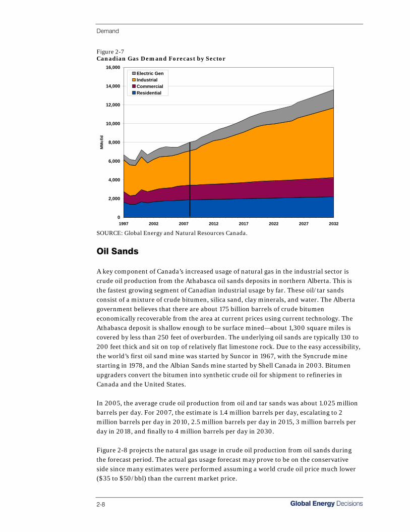
Demand
2-8
Figure 2-7 Canadian Gas Demand Forecast by Sector
0
2,000
4,000
6,000
8,000
10,000
12,000
14,000
16,000
1997 2002 2007 2012 2017 2022 2027 2032
MM
cf/d
Electric GenIndustrialCommercialResidential
SOURCE: Global Energy and Natural Resources Canada.
Oil Sands A key component of Canada’s increased usage of natural gas in the industrial sector is crude oil production from the Athabasca oil sands deposits in northern Alberta. This is the fastest growing segment of Canadian industrial usage by far. These oil/tar sands consist of a mixture of crude bitumen, silica sand, clay minerals, and water. The Alberta government believes that there are about 175 billion barrels of crude bitumen economically recoverable from the area at current prices using current technology. The Athabasca deposit is shallow enough to be surface mined—about 1,300 square miles is covered by less than 250 feet of overburden. The underlying oil sands are typically 130 to 200 feet thick and sit on top of relatively flat limestone rock. Due to the easy accessibility, the world’s first oil sand mine was started by Suncor in 1967, with the Syncrude mine starting in 1978, and the Albian Sands mine started by Shell Canada in 2003. Bitumen upgraders convert the bitumen into synthetic crude oil for shipment to refineries in Canada and the United States. In 2005, the average crude oil production from oil and tar sands was about 1.025 million barrels per day. For 2007, the estimate is 1.4 million barrels per day, escalating to 2 million barrels per day in 2010, 2.5 million barrels per day in 2015, 3 million barrels per day in 2018, and finally to 4 million barrels per day in 2030. Figure 2-8 projects the natural gas usage in crude oil production from oil sands during the forecast period. The actual gas usage forecast may prove to be on the conservative side since many estimates were performed assuming a world crude oil price much lower ($35 to $50/bbl) than the current market price.
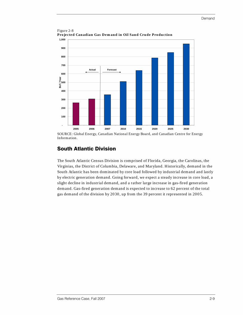
Demand
Gas Reference Case, Fall 2007 2-9
Figure 2-8 Projected Canadian Gas Demand in Oil Sand Crude Production
-
100
200
300
400
500
600
700
800
900
1,000
2005 2006 2007 2010 2015 2020 2025 2030
Bcf
/ Ye
ar
ForecastActual
SOURCE: Global Energy, Canadian National Energy Board, and Canadian Centre for Energy Information.
South Atlantic Division The South Atlantic Census Division is comprised of Florida, Georgia, the Carolinas, the Virginias, the District of Columbia, Delaware, and Maryland. Historically, demand in the South Atlantic has been dominated by core load followed by industrial demand and lastly by electric generation demand. Going forward, we expect a steady increase in core load, a slight decline in industrial demand, and a rather large increase in gas-fired generation demand. Gas-fired generation demand is expected to increase to 62 percent of the total gas demand of the division by 2030, up from the 39 percent it represented in 2005.
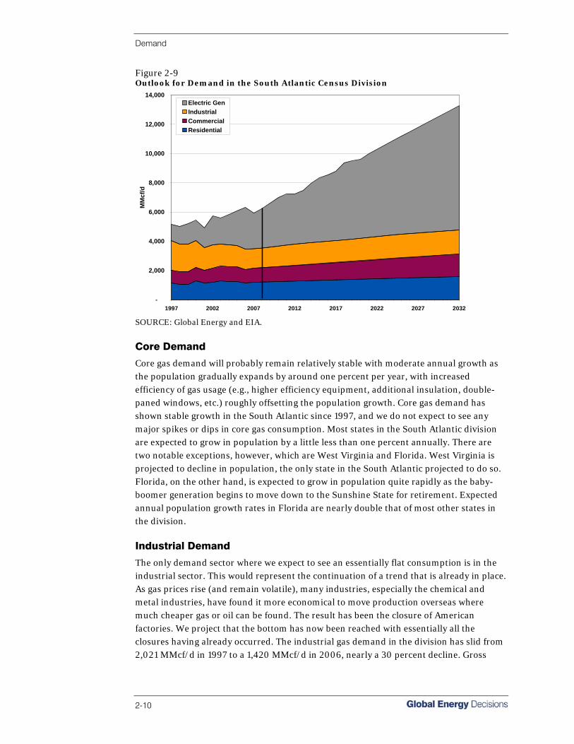
Demand
2-10
Figure 2-9 Outlook for Demand in the South Atlantic Census Division
-
2,000
4,000
6,000
8,000
10,000
12,000
14,000
1997 2002 2007 2012 2017 2022 2027 2032
MM
cf/d
Electric GenIndustrial CommercialResidential
SOURCE: Global Energy and EIA.
Core Demand
Core gas demand will probably remain relatively stable with moderate annual growth as the population gradually expands by around one percent per year, with increased efficiency of gas usage (e.g., higher efficiency equipment, additional insulation, double-paned windows, etc.) roughly offsetting the population growth. Core gas demand has shown stable growth in the South Atlantic since 1997, and we do not expect to see any major spikes or dips in core gas consumption. Most states in the South Atlantic division are expected to grow in population by a little less than one percent annually. There are two notable exceptions, however, which are West Virginia and Florida. West Virginia is projected to decline in population, the only state in the South Atlantic projected to do so. Florida, on the other hand, is expected to grow in population quite rapidly as the baby-boomer generation begins to move down to the Sunshine State for retirement. Expected annual population growth rates in Florida are nearly double that of most other states in the division. Industrial Demand
The only demand sector where we expect to see an essentially flat consumption is in the industrial sector. This would represent the continuation of a trend that is already in place. As gas prices rise (and remain volatile), many industries, especially the chemical and metal industries, have found it more economical to move production overseas where much cheaper gas or oil can be found. The result has been the closure of American factories. We project that the bottom has now been reached with essentially all the closures having already occurred. The industrial gas demand in the division has slid from 2,021 MMcf/d in 1997 to a 1,420 MMcf/d in 2006, nearly a 30 percent decline. Gross
Demand
Gas Reference Case, Fall 2007 2-11
State Product (GSP) for the South Atlantic is expected to show a relatively consistent growth rate of around 4 percent. Electric Generation Demand
The most striking feature of the demand growth forecast for the South Atlantic census division is the expected major increase in demand from the electric generation (EG) sector. This is a result of new gas-fired power plants being built in the division. The majority of the new power generation built nationally in the last few years has been gas-fired, and this is certainly the case in the South Atlantic. From 1997 to 2001, consumption for EG was steady and displayed little if any growth. Then, in 2002, demand shot from 1,382 MMcf/d the year before to 1,982 MMcf/d. EG consumption was up again in 2005 to 2,379 MMcf/d and jumped to 2,840 MMcf/day in 2006. As stated in prior Reference Cases, the growth trend is very likely to continue. We anticipate an especially substantial jump in gas consumption for EG occurring in the next several years during which we expect to see average annual demand increasing by over 5 percent. By 2030, the forecasted EG demand for the division will reach nearly 8 Bcf/d, nearly a 10 percent average growth rate. The South Atlantic is one of two divisions that have a relatively high capacity for switching fuel used for power generation. Should the price of gas become exceptionally high relative to oil, some EG gas demand has the potential to be replaced by oil. In 2004, 113 MMcf/d of power generation could be switched between gas and oil. Power generators in the South Atlantic tend to switch some capacity from gas-fired generation to light oil-fired generation when the price differential between the two fuels is at or under $0.50-$1/MMBtu, depending on the price of SO2 allowances.
Middle Atlantic Division New Jersey, New York, and Pennsylvania are the states that make up the Middle Atlantic census division. In the past, the division has seen strong demand from the core sector, which has made up close to two-thirds of the overall gas consumption. The remaining demand has been split almost evenly between power generation and industrial consumption. Going forward, we expect to see continued growth in core gas demand, although the sector will make up a smaller percentage of total demand. EG demand is anticipated to increase considerably while industrial demand falls.

Demand
2-12
Figure 2-10 Outlook for Demand in the Middle Atlantic Census Division
-
1,000
2,000
3,000
4,000
5,000
6,000
7,000
8,000
9,000
10,000
1997 2002 2007 2012 2017 2022 2027 2032
MM
cf/d
Electric GenIndustrial CommercialResidential
SOURCE: Global Energy and EIA.
Core Demand
One characteristic of the Middle Atlantic division that has been true since 1997—and we expect to remain strong—is core sector demand making up a large percentage of the division’s overall gas consumption. For the last several years, core demand in the Middle Atlantic has hovered at or around 4,000 MMcf/d. By 2030, we anticipate that very gradual increases in core consumption during most years will increase core gas demand to 4,400 MMcf/d. However, while core gas consumption represented 62 percent of the division’s demand in 2000, we anticipate it will only account for 50 percent by 2030. Industrial Demand
The Middle Atlantic division demonstrates a nation-wide trend of declining industrial gas demand. As is the case in most of the country, persistently high natural gas prices have forced the closures of many industrial plants since the gas they need can be found much cheaper elsewhere. The largest declines in industrial consumption have already occurred and have likely bottomed out. From 2000 to 2006, the industrial sector in the division has been losing about 3.1 percent of its annual demand on average. However, from 2006 to 2030 we believe consumption by the industrial sector will very gradually rise by 0.9 percent annually on average as projected consumption rates go from 927 MMcf/d up to 1,124 MMcf/d. Electric Generation Demand
The largest expected growth in gas demand in percentage terms over the next 25 years will probably be seen in the EG sector. From 2007 to 2030, we expect a sizable 3.9 percent average yearly increase in EG consumption for the Middle Atlantic division. EG

Demand
Gas Reference Case, Fall 2007 2-13
demand in 2005 stood at 1,403 MMcf/d and increased over 23 percent to 1,731 MMcf/d in 2006. By 2030, we expect to see EG demand climb to 3,331 MMcf/d. The Middle Atlantic is one of two census divisions that often see considerable fuel switching between gas and oil for EG. Should the price of gas become exceptionally high relative to oil, a potential 460 MMcf/d of fuel for power generation would be able to switch between gas and oil as of 2007. Much like in the South Atlantic division, fuel switching becomes a major consideration when the price differential between natural gas and light oil goes under $ 1. This means that if gas prices soar, the potential to destroy some EG demand in the Middle Atlantic division is a possibility. We are expecting to see gross state product (GSP) in the division expand at a rate just under 3 percent over the next 25 years. We also anticipate seeing total gas consumption for the Middle Atlantic increase by about 1.4 percent annually. Those two figures stand to support each other given the usual correlation between gas demand and a growing GSP.
New England Division The New England census division is made up of Connecticut, Maine, Massachusetts, New Hampshire, Rhode Island, and Vermont. Historically, the bulk of demand in this division has come from the core sector, which in 2000 accounted for roughly half the division’s consumption. EG demand has seen steady growth over the last few years while industrial demand has been in a gradual decline. Over the following years we expect to see dramatic demand growth from the EG sector. We are also forecasting a return to demand growth from the industrial sector and very slow core sector demand, being aided by the higher-than-average per capita income for this division. Figure 2-11 Outlook for Demand in the New England Census Division
-
500
1,000
1,500
2,000
2,500
3,000
3,500
4,000
1997 2002 2007 2012 2017 2022 2027 2032
MM
cf/d
Electric GenIndustrial CommercialResidential
SOURCE: Global Energy and EIA.
Demand
2-14
Core Demand
Core gas consumption in New England has ranged from 758 to 975 MMcf/d since 1997. We forecast a gradual increase in core gas consumption (by 1.3 percent annually) to continue over the next 25 years as the population increases modestly at about 0.5 percent each year in the New England division. Industrial Demand
High gas prices have hurt New England’s industrial demand for gas. The industrial sector’s consumption peaked in 1999 at 429 MMcf/d, which at the time represented 24 percent of overall natural gas demand in New England. By 2006 total industrial demand stood at 221 MMcf/d, which is only 11 percent of overall demand. Global Energy’s forecast projects that lower prices and economic growth will bring back industrial demand to about seven-eighths of its former level. Electric Generation Demand
Like in many other census divisions, New England natural gas demand growth is expected to be driven by the EG sector. Traditionally a region that was mainly reliant on residual fuel oil (ranging from 0.5 percent sulfur up to 2 percent sulfur) for its intermediate cycling electric generation usage, from 1997 to 2006 New England saw a steady increase in gas consumption with demand nearly doubling over that time span from 559 MMcf/d to 1,008 MMcf/d. Now much of the gas demand is for base loaded, combined cycle gas turbines. We expect to see this trend continuing through the end of the forecast period, reaching nearly 2.3 Bcf/d in 2030. Overall, EG demand growth is projected to average a very strong 5.4 percent during the forecast period.
East North Central Division The East North Central census division is comprised of Indiana, Illinois, Michigan, Ohio, and Wisconsin. Historically, core demand has made up nearly two-thirds of overall gas consumption with industrial demand making up most of the other third. Power generation has been a minor contributor to gas demand in the division since this region has large amounts of inexpensive coal-fired generation. Looking forward, we expect to see only little growth from core users and fair growth from industrials and electric generation.
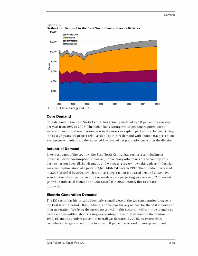
Demand
Gas Reference Case, Fall 2007 2-15
Figure 2-12 Outlook for Demand in the East North Central Census Division
-
2,000
4,000
6,000
8,000
10,000
12,000
14,000
1997 2002 2007 2012 2017 2022 2027 2032
MM
cf/d
Electric GenIndustrial CommercialResidential
SOURCE: Global Energy and EIA.
Core Demand
Core demand in the East North Central has actually declined by 1.8 percent on average per year from 1997 to 2006. The region has a strong winter peaking requirement so warmer than normal weather one year to the next can explain part of this change. During the next 25 years, we project relative stability in core demand with about a 0.8 percent on average growth mirroring the expected low level of net population growth in the division. Industrial Demand
Like most parts of the country, the East North Central has seen a recent decline in industrial sector consumption. However, unlike many other parts of the country, this decline has not been all that dramatic and we see a recovery now taking place. Industrial gas consumption stood at a peak of 3,676 MMcf/d back in 1997. That number decreased to 3,078 MMcf/d by 2006, which is not as steep a fall in industrial demand as we have seen in other divisions. From 2007 onwards we are projecting an average of 2.2 percent growth in industrial demand to 4,709 MMcf/d in 2030, mainly due to ethanol production. Electric Generation Demand
The EG sector has historically been only a small piece of the gas consumption picture in the East North Central. Ohio, Indiana, and Wisconsin rely on coal for the vast majority of their generation. While we do anticipate growth in this sector, it will continue to make up only a modest—although increasing—percentage of the total demand in the division. In 1997, EG made up only 6 percent of overall gas demand. By 2015, we expect EG’s contribution to gas consumption to grow to 8 percent as a result of new power plant
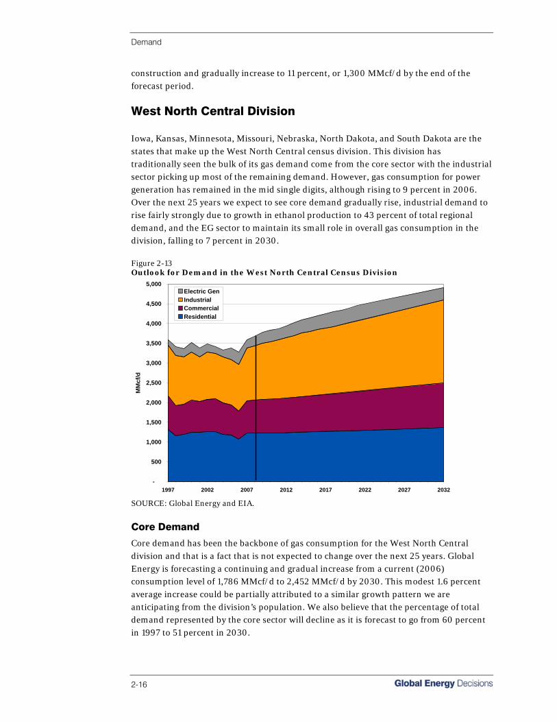
Demand
2-16
construction and gradually increase to 11 percent, or 1,300 MMcf/d by the end of the forecast period.
West North Central Division Iowa, Kansas, Minnesota, Missouri, Nebraska, North Dakota, and South Dakota are the states that make up the West North Central census division. This division has traditionally seen the bulk of its gas demand come from the core sector with the industrial sector picking up most of the remaining demand. However, gas consumption for power generation has remained in the mid single digits, although rising to 9 percent in 2006. Over the next 25 years we expect to see core demand gradually rise, industrial demand to rise fairly strongly due to growth in ethanol production to 43 percent of total regional demand, and the EG sector to maintain its small role in overall gas consumption in the division, falling to 7 percent in 2030. Figure 2-13 Outlook for Demand in the West North Central Census Division
-
500
1,000
1,500
2,000
2,500
3,000
3,500
4,000
4,500
5,000
1997 2002 2007 2012 2017 2022 2027 2032
MM
cf/d
Electric GenIndustrial CommercialResidential
SOURCE: Global Energy and EIA.
Core Demand
Core demand has been the backbone of gas consumption for the West North Central division and that is a fact that is not expected to change over the next 25 years. Global Energy is forecasting a continuing and gradual increase from a current (2006) consumption level of 1,786 MMcf/d to 2,452 MMcf/d by 2030. This modest 1.6 percent average increase could be partially attributed to a similar growth pattern we are anticipating from the division’s population. We also believe that the percentage of total demand represented by the core sector will decline as it is forecast to go from 60 percent in 1997 to 51 percent in 2030.
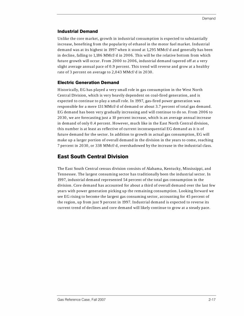
Demand
Gas Reference Case, Fall 2007 2-17
Industrial Demand
Unlike the core market, growth in industrial consumption is expected to substantially increase, benefiting from the popularity of ethanol in the motor fuel market. Industrial demand was at its highest in 1997 when it stood at 1,295 MMcf/d and generally has been in decline, falling to 1,186 MMcf/d in 2006. This will be the relative bottom from which future growth will occur. From 2000 to 2006, industrial demand tapered off at a very slight average annual pace of 0.9 percent. This trend will reverse and grow at a healthy rate of 3 percent on average to 2,043 MMcf/d in 2030. Electric Generation Demand
Historically, EG has played a very small role in gas consumption in the West North Central Division, which is very heavily dependent on coal-fired generation, and is expected to continue to play a small role. In 1997, gas-fired power generation was responsible for a mere 131 MMcf/d of demand or about 3.7 percent of total gas demand. EG demand has been very gradually increasing and will continue to do so. From 2006 to 2030, we are forecasting just a 10 percent increase, which is an average annual increase in demand of only 0.4 percent. However, much like in the East North Central division, this number is at least as reflective of current inconsequential EG demand as it is of future demand for the sector. In addition to growth in actual gas consumption, EG will make up a larger portion of overall demand in the division in the years to come, reaching 7 percent in 2030, or 338 MMcf/d, overshadowed by the increase in the industrial class.
East South Central Division The East South Central census division consists of Alabama, Kentucky, Mississippi, and Tennessee. The largest consuming sector has traditionally been the industrial sector. In 1997, industrial demand represented 54 percent of the total gas consumption in the division. Core demand has accounted for about a third of overall demand over the last few years with power generation picking up the remaining consumption. Looking forward we see EG rising to become the largest gas consuming sector, accounting for 45 percent of the region, up from just 9 percent in 1997. Industrial demand is expected to reverse its current trend of declines and core demand will likely continue to grow at a steady pace.
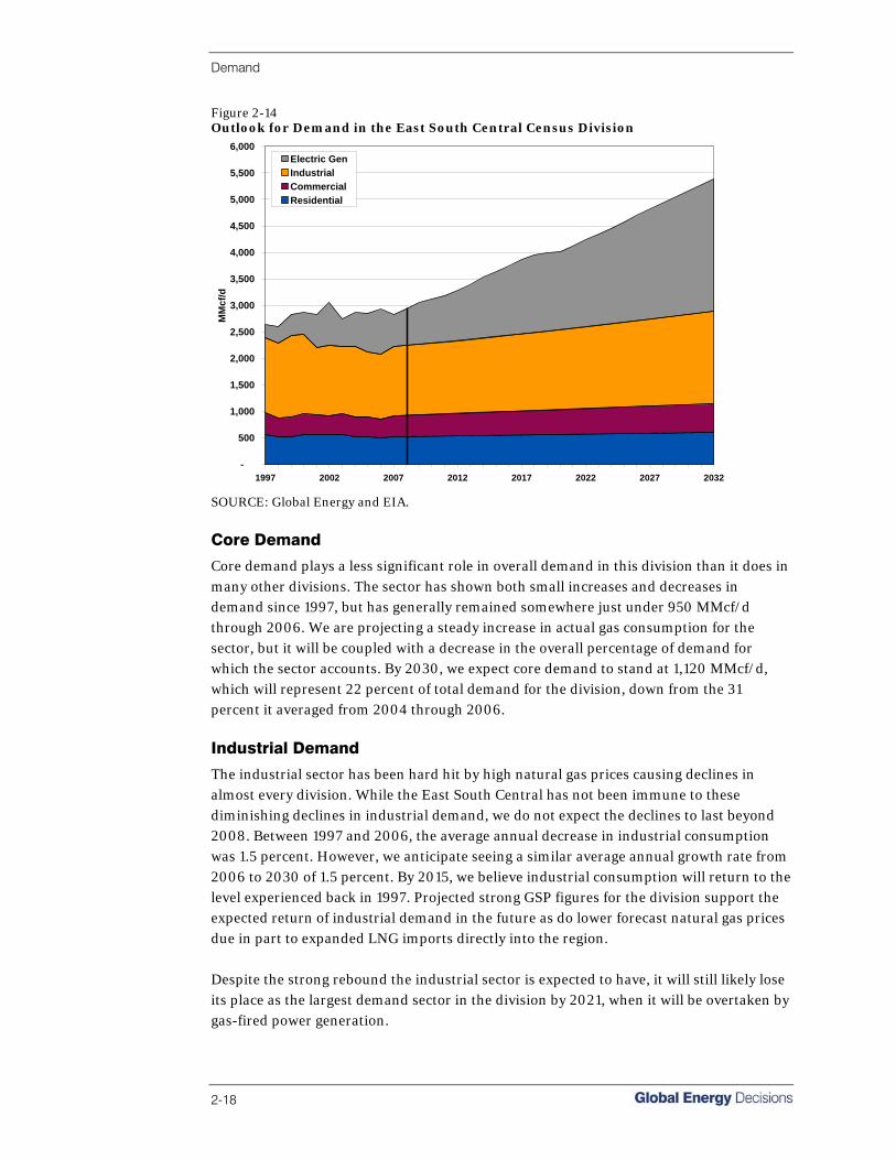
Demand
2-18
Figure 2-14 Outlook for Demand in the East South Central Census Division
-
500
1,000
1,500
2,000
2,500
3,000
3,500
4,000
4,500
5,000
5,500
6,000
1997 2002 2007 2012 2017 2022 2027 2032
MM
cf/d
Electric GenIndustrial CommercialResidential
SOURCE: Global Energy and EIA.
Core Demand
Core demand plays a less significant role in overall demand in this division than it does in many other divisions. The sector has shown both small increases and decreases in demand since 1997, but has generally remained somewhere just under 950 MMcf/d through 2006. We are projecting a steady increase in actual gas consumption for the sector, but it will be coupled with a decrease in the overall percentage of demand for which the sector accounts. By 2030, we expect core demand to stand at 1,120 MMcf/d, which will represent 22 percent of total demand for the division, down from the 31 percent it averaged from 2004 through 2006. Industrial Demand
The industrial sector has been hard hit by high natural gas prices causing declines in almost every division. While the East South Central has not been immune to these diminishing declines in industrial demand, we do not expect the declines to last beyond 2008. Between 1997 and 2006, the average annual decrease in industrial consumption was 1.5 percent. However, we anticipate seeing a similar average annual growth rate from 2006 to 2030 of 1.5 percent. By 2015, we believe industrial consumption will return to the level experienced back in 1997. Projected strong GSP figures for the division support the expected return of industrial demand in the future as do lower forecast natural gas prices due in part to expanded LNG imports directly into the region. Despite the strong rebound the industrial sector is expected to have, it will still likely lose its place as the largest demand sector in the division by 2021, when it will be overtaken by gas-fired power generation.
Demand
Gas Reference Case, Fall 2007 2-19
Electric Generation Demand
With the plethora of coal-fired generation in the region, EG had traditionally been only a minor contributor to gas consumption in the East South Central division. In 1997, EG demand was only 243 MMcf/d or 9.2 percent of overall demand. Since then, however, consumption by gas-fired power generation has increased quite significantly. EG demand reached a relative peak in 2002 of 801 MMcf/d and another in 2006 of 837 MMcf/d. We expect to see EG demand increase about 177 percent to nearly 2.3 Bcf/d in 2030. This equates to a 7.4 percent annual average rise, comprising 45 percent of overall regional demand.
West South Central Division Arkansas, Louisiana, Oklahoma, and Texas make up the West South Central census division. This division historically has been unique in several ways. First, the West South Central has the highest overall gas demand of any division, which peaked at 16,572 MMcf/d in 2000. Also, core demand makes up an unusually low percentage of overall demand. In 2000, the core demand sector accounted for only 11 percent of total demand. In the past, industrial demand has been the most prominent sector in the division. Lately, industrial demand has been in serious decline, down 28 percent between 1997 and 2006; however, a return to lower gas prices and a share in the surge in ethanol production will keep industrial gas consumption the most significant sector in the region. Most noticeably, in 2005, the impact on industrial demand from Hurricanes Rita and Katrina was most evident when industrial demand reached its perigee of 6,294 MMcf/d from its relative peak of 9,330 MMcf/d in 1997. Figure 2-15 Outlook for Demand in the West South Central Census Division
-
2,000
4,000
6,000
8,000
10,000
12,000
14,000
16,000
18,000
20,000
1997 2002 2007 2012 2017 2022 2027 2032
MM
cf/d
Electric GenIndustrial CommercialResidential
SOURCE: Global Energy and EIA.
Demand
2-20
Core Demand
Core demand represents a smaller and more insignificant piece of the overall demand in this division than in any other. Gas consumption by the core sector peaked in 1997 at 1,968 MMcf/d and has been very gradually declining ever since, reaching 1,428 MMcf/d in 2006. In the future we expect to see the declines to reverse and we expect that a trend of subtle increases from the sector to return. Led by Texas in particular, population is expected to increase a bit more rapidly in this division than in most, and this will likely be the cause of the measured expansion in core demand, averaging 2.8 percent annually to reach 2,406 MMcf/d in 2030. Industrial Demand
The West South Central has traditionally been the largest industrial gas consuming division. Due to the proximity to gas fields and natural gas infrastructure, many chemical, metal, and other industrial gas consuming industries set up plants and factories in the division. This situation is so prevalent in Louisiana that the exceptionally gas rich state is actually a net importer of natural gas. With the high price of gas causing companies to relocate plants overseas, however, industrial demand has been in decline over the last few years. Demand dropped from a high of 9,330 MMcf/d in 1997 to 6,294 MMcf/d in 2005 before rebounding to 6,812 MMcf/d in the post-Rita and Katrina environment. The trend of falling industrial demand is forecast to reverse with decline in gas prices projected. Global Energy expects industrial demand to grow from around 7,700 MMcf/d, given our price projections for the commodity, and then gradually increase at an average rate of 1.2 percent until reaching 8,756 MMcf/d in 2030, benefiting somewhat from the high demand for ethanol since Texas is the tenth largest state currently in terms of ethanol production and more facilities are scheduled to be constructed. Electric Generation Demand
Demand from the EG sector has also been declining from 2000 although it rose in 2005 to 5,495 MMcf/d and again in 2006 to 5,636 MMcf/d, due in part to high electric load demand caused by hot weather. Its historical peak occurred in 2000 at 5,733 MMcf/d. Since then many older, less efficient gas-fired steam turbines have been replaced by more efficient combined cycle generation. Unlike industrial demand though, this is a trend that we do not believe will continue. In fact, we anticipate seeing gas-fired power generation to grow between 2007 through 2030 by 1.7 percent average annually, reaching nearly 7.2 Bcf/d at which time EG demand will comprise 41 percent of overall demand.
Mountain Division The Mountain census division is comprised of Arizona, Colorado, Idaho, New Mexico, Montana, Utah, Nevada, and Wyoming. Historically, core demand has been the largest demand sector; however, in recent years increases in consumption from the EG sector have exceeded combined residential and commercial core demand. Industrial demand has mostly remained steady and is only expected to grow very slowly over the forecast period. Looking forward we forecast an extremely sizable increase in demand coming from the EG sector, up to 3.8 Bcf/d in 2030, making it by far the largest gas consuming
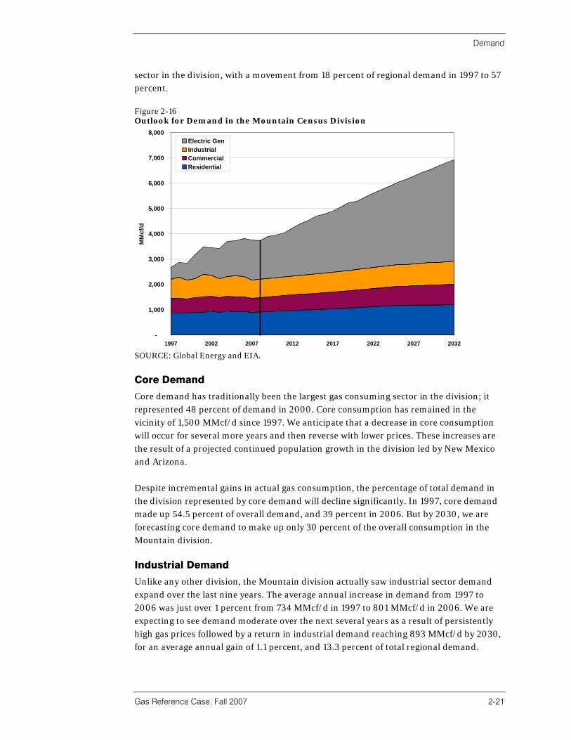
Demand
Gas Reference Case, Fall 2007 2-21
sector in the division, with a movement from 18 percent of regional demand in 1997 to 57 percent. Figure 2-16 Outlook for Demand in the Mountain Census Division
-
1,000
2,000
3,000
4,000
5,000
6,000
7,000
8,000
1997 2002 2007 2012 2017 2022 2027 2032
MM
cf/d
Electric GenIndustrial CommercialResidential
SOURCE: Global Energy and EIA.
Core Demand
Core demand has traditionally been the largest gas consuming sector in the division; it represented 48 percent of demand in 2000. Core consumption has remained in the vicinity of 1,500 MMcf/d since 1997. We anticipate that a decrease in core consumption will occur for several more years and then reverse with lower prices. These increases are the result of a projected continued population growth in the division led by New Mexico and Arizona. Despite incremental gains in actual gas consumption, the percentage of total demand in the division represented by core demand will decline significantly. In 1997, core demand made up 54.5 percent of overall demand, and 39 percent in 2006. But by 2030, we are forecasting core demand to make up only 30 percent of the overall consumption in the Mountain division. Industrial Demand
Unlike any other division, the Mountain division actually saw industrial sector demand expand over the last nine years. The average annual increase in demand from 1997 to 2006 was just over 1 percent from 734 MMcf/d in 1997 to 801 MMcf/d in 2006. We are expecting to see demand moderate over the next several years as a result of persistently high gas prices followed by a return in industrial demand reaching 893 MMcf/d by 2030, for an average annual gain of 1.1 percent, and 13.3 percent of total regional demand.

Demand
2-22
Electric Generation Demand
EG demand has experienced very strong growth between 1997 when demand stood at 482 MMcf/d and 2006 when demand reached 1,522 MMcf/d, a 216 percent increase. Global Energy expects the growth trend to continue unabated through 2030, when projected EG demand for the division will hit 3,794 MMcf/d. In 1997, gas-fired power generation accounted for just 18 percent of overall demand in the division. By 2030, we are projecting the EG sector to represent as much as 57 percent of the Mountain division’s total demand.
Pacific Division California, Oregon, and Washington make up the Pacific census division. Demand in the region has been split almost evenly between the core (residential combined with commercial), industrial, and electric generation sectors. However, we expect all three to show growth in gas demand over the next 25 years, with the smallest growth expected in the industrial sector, which will remain almost flat. The largest demand expansion is coming from the EG sector, which is forecast to represent 45.5 percent of total demand in the division in 2030, up from 26 percent in 1997, and over 5.1 Bcf/day. Figure 2-17 Outlook for Demand in the Pacific Census Division
-
1,000
2,000
3,000
4,000
5,000
6,000
7,000
8,000
9,000
10,000
11,000
12,000
13,000
1997 2002 2007 2012 2017 2022 2027 2032
MM
cf/d
Electric GenIndustrial CommercialResidential
SOURCE: Global Energy and EIA.
Core Demand
In the Pacific division, core demand peaked in 1999 at 2,877 MMcf/d. Since then the demand from the sector has been moderated slightly in most years. By 2030, we are forecasting core demand to reach 3,359 MMcf/d, an average annual increase of 1.5 percent during the forecast period.
Demand
Gas Reference Case, Fall 2007 2-23
Industrial Demand
Over the past several years, just as in most divisions, price sensitive industrial demand has fallen in the Pacific division, down a total of 13 percent since the peak of 2,899 MMcf/d in 1998. And the culprits causing the decline in consumption here are the same as elsewhere. High gas prices have forced the closure of plants and factories in the division. The metal—particularly aluminum—industry has seen a series of plant closures in the Pacific Northwest. Over the next few forecast years we expect to see industrial consumption decline somewhat caused by slower economic growth and persistently high gas prices. However, demand growth comes back into the forecast by 2009. From that year onwards we forecast industrial demand growth of 0.9 percent per year and reach 2,812 MMcf/d by 2030. Electric Generation Demand
The EG sector is where we anticipate seeing the largest growth by far in demand for the Pacific division looking forward. Demand for the sector peaked in 2001 at 3,218 MMcf/d—the California crisis year, brought about by record low hydro power availability. Demand had been falling slightly for a few years since then, but it started climbing again in 2004 and 2006 as well, reaching 2,640 MMcf/d. As is the case with most EG growth in other divisions, we expect to see the fastest expansion of EG demand in percentage terms over the next 25 years. For the division we are forecasting an average annual growth rate of 4 percent from 2006 to 2030. EG demand will have increased from 26 percent of total demand in the division in 1997 to 46 percent of the total in 2030, averaging nearly 5.24 Bcf/d.
Conclusions Overall, U.S. gas demand is projected to rise 4 percent from 55,488 MMcf/d in 2006 to an estimated 57,693 MMcf/d in 2007, upward to 83,796 MMcf/d by 2030. This represents an overall increase of 2.1 percent annually. Looking at it another way, due to the expected rapid growth in power generation fuel demand, the next 25-year period will see an unprecedented rate of growth. Electric generation demand will more than double during the forecast period from 14.7 Bcf/d to 33.7 Bcf/d or 5.4 percent annually. Given current high gas prices and the current state of conventional gas resources across North America, this will challenge the gas supply industry and will provide many new investment opportunities. Global Energy believes that the majority of the incremental gas supply will come in the form of LNG as well as from various unconventional and frontier sources. These are discussed in Sections 3 and 4 of this report. However, we recognize that demand might not materialize as projected in the Reference Case. Global Energy views the potential magnitude of the forecast error to vary by sector. Our analysis indicates that core gas demand tends to be more easily forecasted due to predictable seasonal weather and the homogeneous use of gas (mostly for heating) in this sector. Of course, harsh or warm winters can and do drive short-term delivery shortages, which raise price volatility. But over five or more years, these weather patterns tend to normalize and offset each other. Population growth, commercial and residential floor space, price elasticity, and energy efficiency then become the driving factors of core

Demand
2-24
demand growth. All of these factors tend to be fairly steady and predictable, since the adoption of future energy saving devices tends to be measured. Industrial gas demand tends to be much more price sensitive and therefore less certain over time. The industrial sector tends to respond to changes in price more rapidly as well. The adoption of new energy-saving technologies has the potential of reducing energy bills; however, a comprehensive engineering industry-by-industry review would be necessary to fully assess this potential and is beyond the scope of this report. New and expanded uses for natural gas, such as for crude production from oil sands and ethanol production from corn, becomes a positive driver of demand, perhaps more than offsetting energy efficiency gains and having old “rust belt” industries move overseas. Finally, the electric generation sector is perhaps the least certain demand sector to project growth for. This is primarily driven by three factors. First, this is the source of the strongest demand growth and by definition, the forecast change in demand between 2007 and 2030 is the largest. Second, fuel substitutes exist for power generation in the form of coal, nuclear, and renewables, although over the next five to seven years it is unlikely that significant alternative generation resources could be built, due to the long permitting and construction times required. Third, significant efficiency gains through potential mandated energy-efficiency technologies are possible, such as for lighting, air-conditioning, heating, and insulation. Beyond 2012, given the right price incentives and a favorable regulatory environment, that could change. Of course new coal and nuclear plants face many hurdles. In addition, the price of uranium has been increasingly volatile recently. It is for this reason that many developers chose to build gas combined cycle plants almost exclusively over the past five years. Prior to 2010, Global Energy believes that forecast uncertainty for power generation gas demand will be less due to the present amount of underutilized gas-fired generation. Several forecast “wildcards” do exist which will affect demand. If new LNG gas supply and liquefaction facilities (discussed in Sections 3 and 4) do not materialize in a timely fashion as expected in this forecast, Global Energy would expect that very high market prices would ensue for a number of years. Just how high prices would rise is difficult to quantify since unprecedented scarcity premiums and demand responses would certainly occur. Additionally, LNG is rapidly becoming a global commodity with many nations bidding for short- and long-term supply. However, all of the price sensitive demand sectors (industrial in the short run and electric generation in the longer run) and core demand would be affected. This would lead to more industrial plant closures and increasing repowering efforts towards lower cost, solid fuel power plants with markedly different and lasting gas demand impacts. Alternatively, excess LNG supply would have the effect of reducing prices (at least temporarily) as LNG floods the marketplace. Basis differentials will change accordingly. Regasified LNG during the summer months can be used to inject gas into underground storage fields, thus changing seasonal basis as well. If gas consumers believe excess LNG
Demand
Gas Reference Case, Fall 2007 2-25
supply conditions represent a new equilibrium price, then both gas demand and energy conservation will be impacted in the short run and investment decisions to build new plants in the long run. Another “wildcard” is future emission regulation and policy. Global Energy utilizes the Clean Air Interstate Rule (CAIR) and the Regional Greenhouse Gas Initiative (RGGI) in its electric market forecast; however, we have not incorporated any additional proposed greenhouse gas (GHG) regulations. In the present political environment in the United States, this seems reasonable; however, things could change dramatically in the near future. (For more information, see Appendix J on Legislative Initiatives on Carbon Trading.) If more emphasis on carbon emission reductions materializes through regulation, then all sectors of the economy will be affected. Given the lack of viable alternatives, natural gas will be seen by many as the key “bridge fuel” taking up much of the incremental fuel demand growth. In Canada, this is precisely what has happened. Canada, which ratified the Kyoto agreement, now faces many difficult energy policy and implementation decisions. For example, Ontario has chosen to shut down its entire coal-fired generation fleet (over 7,000 MW). Repowering options are leaning heavily on new gas construction and restarting several nuclear power plants. In Global Energy’s opinion, this will place an additional premium on gas market prices regionally.


Section 3 | Supply

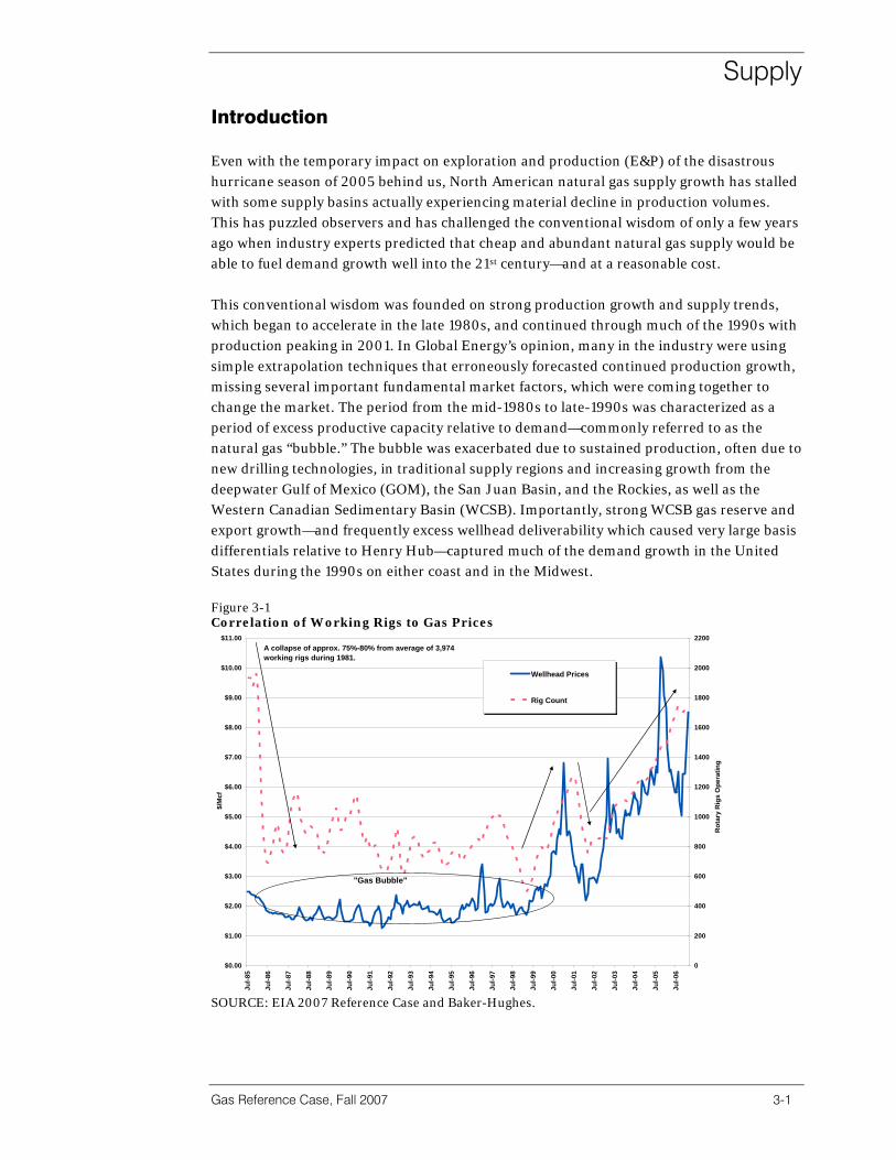
Supply
Gas Reference Case, Fall 2007 3-1
Introduction Even with the temporary impact on exploration and production (E&P) of the disastrous hurricane season of 2005 behind us, North American natural gas supply growth has stalled with some supply basins actually experiencing material decline in production volumes. This has puzzled observers and has challenged the conventional wisdom of only a few years ago when industry experts predicted that cheap and abundant natural gas supply would be able to fuel demand growth well into the 21st century—and at a reasonable cost. This conventional wisdom was founded on strong production growth and supply trends, which began to accelerate in the late 1980s, and continued through much of the 1990s with production peaking in 2001. In Global Energy’s opinion, many in the industry were using simple extrapolation techniques that erroneously forecasted continued production growth, missing several important fundamental market factors, which were coming together to change the market. The period from the mid-1980s to late-1990s was characterized as a period of excess productive capacity relative to demand—commonly referred to as the natural gas “bubble.” The bubble was exacerbated due to sustained production, often due to new drilling technologies, in traditional supply regions and increasing growth from the deepwater Gulf of Mexico (GOM), the San Juan Basin, and the Rockies, as well as the Western Canadian Sedimentary Basin (WCSB). Importantly, strong WCSB gas reserve and export growth—and frequently excess wellhead deliverability which caused very large basis differentials relative to Henry Hub—captured much of the demand growth in the United States during the 1990s on either coast and in the Midwest. Figure 3-1 Correlation of Working Rigs to Gas Prices
$0.00
$1.00
$2.00
$3.00
$4.00
$5.00
$6.00
$7.00
$8.00
$9.00
$10.00
$11.00
Jul-8
5
Jul-8
6
Jul-8
7
Jul-8
8
Jul-8
9
Jul-9
0
Jul-9
1
Jul-9
2
Jul-9
3
Jul-9
4
Jul-9
5
Jul-9
6
Jul-9
7
Jul-9
8
Jul-9
9
Jul-0
0
Jul-0
1
Jul-0
2
Jul-0
3
Jul-0
4
Jul-0
5
Jul-0
6
$/M
cf
0
200
400
600
800
1000
1200
1400
1600
1800
2000
2200
Rot
ary
Rig
s O
pera
ting
Wellhead Prices
Rig Count
A collapse of approx. 75%-80% from average of 3,974 working rigs during 1981.
"Gas Bubble"
SOURCE: EIA 2007 Reference Case and Baker-Hughes.

Supply
3-2
More recently, North American production has been essentially flat, plus or minus 1 to 2 percent since 2001, though during this period replacement of proved in-ground reserves has generally ranged from 110 percent to 140 percent of the annual wellhead production. This is especially true in Canada where recent years have seen flat or declining WCSB production and declining exports to the United States as annual production was continuously replaced with proved in-ground reserves. In fact, the U.S. producers have a five-year rolling average reserve replacement of 165 percent; 215 percent during 2005. In addition, in August 2005, the U.S. Geological Survey (USGS) reported that between 1996 and 2003 reserves added from infill drilling and secondary and tertiary recovery of existing fields were three times as great as added from new drilling. The USGS said that because of this in-ground reserve growth approximately 30 percent more was added to their mean estimate of proved domestic gas reserves. The GOM remains a key supply point due to its major production volumes and deepwater drilling that must be performed to maintain production from this area. Figure 3-2 U.S Gulf of Mexico Gas Production and Working Gas Rigs
0
100
200
300
400
500
600
Jan-
01
Apr
-01
Jul-0
1
Oct
-01
Jan-
02
Apr
-02
Jul-0
2
Oct
-02
Jan-
03
Apr
-03
Jul-0
3
Oct
-03
Jan-
04
Apr
-04
Jul-0
4
Oct
-04
Jan-
05
Apr
-05
Jul-0
5
Oct
-05
Jan-
06
Apr
-06
Jul-0
6
Oct
-06
Jan-
07
Apr
-07
Jul-0
7
Bcf
/ M
onth
0
25
50
75
100
125
150
GO
M W
orki
ng G
as R
ig C
ount
GOM Gas Production
GOM Gas RigsHurricanes Katrina and Rita, and subsequent repair of damaged rigs, cut the working rigcount and gas production by more than 50%
SOURCE: Global Energy, EIA and Baker-Hughes.
Why did production capacity fail to keep up with reserve replacement capacity? There are several reasons. Largely because investment capital in foreign investment provided better returns, but also due to the volatility and uncertainty in the sustainable wellhead prices needed to drill for indigenous gas, largely unconventional supplies (see Table 3-1). In addition, the unconventional supplies, particularly Rocky Mountain coal bed methane, will largely compete against LNG imports with lower long-run marginal costs as the major source of incremental supply. Finally, many of these new reserve pockets do not have the daily production deliverability that the older “elephant” gas fields possessed when they were first brought on line.

Supply
Gas Reference Case, Fall 2007 3-3
Table 3-1 Domestic Gas Production (Tcf)
Source 2005 (18.2 Tcf) %
2030 (21.7 Tcf) %
Lower 48
1. Unconventional 42 50
2. Non-associated onshore conventional 26 18
3. Non-associated offshore conventional 19 12
4. Associated gas with lower 48 crude 13 9
5. Subtotal 100 89
Alaska 0 11
Total 100 100
SOURCE: Global Energy and EIA 2007 Reference Case.
Therefore, many large producers have turned their attention away from GOM and other U.S. basins towards international exploration and development where the size of reserves and economic returns, as well as per-unit cost of recovery, are much more favorable than in North America. This industry shift to infill and development of existing fields only maintained production during the period of low gas prices; this is not a result of replacing in-ground reserves but is due to relative project economics. This has meant that for the first time, the higher commodity prices and higher company cash flows have not led to a proportional increase in capital spending in North America by many oil and gas producers. This lag in committing capital has helped to fuel a sustained rise in market prices, caused significant new interest in developing marine LNG terminals, and spurred development of Frontier Arctic gas for export by pipeline. Many of these large-scale mega-projects will translate into incremental supply for North America; however, substantial supply deliverability contributions from LNG are not likely to materialize until the 2008-2009 time frame, and Alaskan gas over a decade from now. Furthermore, the extent to which LNG can become a major source of supply for North America rests on the industry’s ability to overcome regulatory hurdles and domestic opposition to siting LNG terminals, and to develop or contract dedicated liquefaction trains for the North American market in a timely manner. Higher wellhead prices and industry cash flow have allowed smaller domestic producers, without much participation in overseas projects, to embark on an aggressive development path. As a result, rig counts have increased substantially in mature producing regions such as those in Texas, Oklahoma, and New Mexico, and in unconventional basins in Texas, Wyoming, Colorado, Utah, and Michigan. The following map and table outlines USGS data on location and possible reserves of unconventional gas reserves.
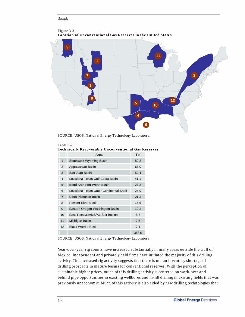
Supply
3-4
Figure 3-3 Location of Unconventional Gas Reserves in the United States
6
2
12
4
5 10
11
9
1
7
8
3
SOURCE: USGS, National Energy Technology Laboratory.
Table 3-2 Technically Recoverable Unconventional Gas Reserves
Area Tcf
1 Southwest Wyoming Basin 82.2
2 Appalachian Basin 66.0
3 San Juan Basin 50.4
4 Louisiana-Texas Gulf Coast Basin 41.1
5 Bend Arch-Fort Worth Basin 26.2
6 Louisiana-Texas Outer Continental Shelf 25.0
7 Uinta-Piceance Basin 21.2
8 Powder River Basin 15.5
9 Eastern Oregon-Washington Basin 12.2
10 East Texas/LA/MS/AL Salt Basins 8.7
11 Michigan Basin 7.5
12 Black Warrior Basin 7.1
363.0
SOURCE: USGS, National Energy Technology Laboratory.
Year-over-year rig counts have increased substantially in many areas outside the Gulf of Mexico. Independent and privately held firms have initiated the majority of this drilling activity. The increased rig activity suggests that there is not an inventory shortage of drilling prospects in mature basins for conventional reserves. With the perception of sustainable higher prices, much of this drilling activity is centered on work-over and behind pipe opportunities in existing wellbores and in-fill drilling in existing fields that was previously uneconomic. Much of this activity is also aided by new drilling technologies that
Supply
Gas Reference Case, Fall 2007 3-5
accelerate production rates and lower unit costs. Unconventional reserves will have low production rates, but will enjoy shallow decline rates and a long production life with average wellhead net-back prices in the $3.50 to $4.00/MMBtu range (2007$). In the absence of new basins to explore, it is new technology that dominates today’s North American exploration industry. Spurred by sustained and projected high gas and oil prices, and the ready availability of highly sophisticated PC-based workstations, high technology geophysics now feature such advances as 3-D seismic using pattern recognition, active-source electromagnetics (which distinguishes water, oil, and gas), and full-wave imaging (which gives a clearer view of subsurface structures than previously available). New drilling and completion technologies developed during the late 1990s, such as horizontal drilling and efficient downhole drilling motors (from <2” diameter to > 11” diameter), are thriving in today’s high-priced market. In the Hartshorne coal bed methane play in the Arkoma Basin of eastern Oklahoma, for example, some 30 operators now utilize horizontal drilling to overcome the long-standing economic challenge of producing gas from the bituminous-rank (low Btu content) coal seams. Leading operators there state that horizontal wells deliver five times the gas volume of a vertical well for two to three times the cost. In the Maverick Basin of southern Texas, a combination of advanced 3-D seismic processing and horizontal drilling kicked off new successes in gas-rich Georgetown carbonates. And reprocessing old 3-D seismic data with new techniques in the shallow-water Louisiana Lake Pelto area has revitalized a field, giving it an estimated additional 15 years of production with a relatively flat decline rate.1 U.S. gas production from conventional stripper wells, which produce 1.5 Tcf/year (approximately 7 percent of U.S. gas production in 2003) is also benefiting from new technology as well as tax incentives. A DOE-backed consortium recently delivered six new commercially ready stripper-well technologies for use by the industry. Eleven states including Louisiana and Texas have gone further giving tax relief for periods ranging from one to ten years to help restore production to inactive wells. Despite the recent drilling and technology boom, which greatly and successfully replaced in-ground proved reserves, in Global Energy’s opinion the result will largely be production maintenance in the range of 50-55 Bcf/day over the forecast period rather than providing significant incremental production capacity. As greater percentages come from unconventional reserves, the result will be more expensive production as the unit-cost increases along with demand growth. Therefore, successful replacement of in-ground reserves will not necessarily alleviate high prices. The economics of accelerating production of unconventional reserves will be compared against imported LNG with lower marginal cost for both incremental supply as well as daily production from cryogenic storage. But a key question remains: can the projected decline in offshore GOM production be offset by an increase in onshore, unconventional LNG and frontier Arctic gas? Once on the fringe of the natural gas industry, unconventional gas sources are quickly growing and expected to contribute 50 percent of domestic gas production in 2030. Unconventional U.S. gas
1 Oil & Gas Investor, June 2005, Page 47.

Supply
3-6
production has increased more than two and a half times between 1990 and 2005, from 2.8 Tcf to 7.5 Tcf. The exhaustion of conventional gas sources will be supplemented in the future with imported LNG and unconventional gas. Whereas conventional natural gas production has centered on porous sandstone and carbonate rock formations, increasingly E&P companies are turning to low-permeability, tight gas sandstones, gas shales, and coal bed methane formations to increase our nation’s natural gas reserves. Conventional gas reservoirs are typically smaller and/or more difficult to locate. On the other hand, these reservoirs can exist over a large area, sometimes already penetrated by older conventional wells, thus reducing the exploration risk. Figure 3-4 shows historic and forecasted production from unconventional reserves. Figure 3-4 Unconventional Gas Production: Volume and Share of Domestic Production
0
2
4
6
8
10
12
1990 1998 2005 2030
Tcf P
rodu
ctio
n
0%
10%
20%
30%
40%
50%
60%
Perc
ent S
hare
of D
omes
tic P
rodu
ctio
n
Annual Production
Share of Domestic Production
Forecast
SOURCE: Global Energy and EIA.
Horizontal drilling techniques may enhance and extend production of unconventional natural gas. Other technologies have been specifically created to better explore for, drill for, complete wells, and produce gas from unconventional reserves. These include advancements in geology/technology modeling, more effective well completion, and stimulation technology such as cavitation and hydraulic fracturing, microseismic monitoring, and enhanced coal bed methane/shales recovery using nitrogen and carbon dioxide injection. The remainder of this section is organized as follows: Supply Methodology discusses basin supply cost curves used to develop our fundamental market forecast; the North American supply picture is then discussed which shows trends in gas supply and production since 1997 to the present time; and the North American supply forecast discusses total gas supply
Supply
Gas Reference Case, Fall 2007 3-7
and production through 2030, supply trends at North American production basins, and frontier and LNG supply growth projections.
Supply Methodology Global Energy’s analysis considers competitive supply costs for incremental gas resources in all major supply basins. We define supply cost as the incremental cost of production in a basin or field. The lowest cost is gas already treated, gathered, processed, and connected to the pipeline where the only production cost component is the lease operating expenses. The next lowest supply sources come from undeveloped proved gas where additional capital investment is required for production and then undeveloped unproved (probable) gas where significantly more expenditure is required and where supply cost and production level uncertainty is larger. Wellhead capacity, or production capacity, is defined as actual production at the wellhead, which is often constrained by gathering and by off-lease processing and transportation capacity in the gas supply delivery chain. Finally, deliverability is defined as the actual gas volumes that can be delivered to the local distribution company (LDC) citygate or to an off-system delivery point. For new reserves, natural gas supply cost is equal to its full cycle replacement cost, which varies significantly by basin due to many factors. The components of this replacement cost will include: • Exploration costs: land, drilling, geological, and geophysical costs including their tax
treatment; • Development costs: drilling and on-lease facilities for gathering and treatment,
including write down and impairments;2 • Accounting methods for depreciation, depletion, and amortization (DD&A); • Production costs (also called lease operating expenses or LOE) including well
workovers, chemicals, power, labor; • Interest costs on any debt burden; • General and administrative expenses (G&A); • Governmental costs such as royalties or carried working interest burdens, production
severance tax, Ad Valorem taxes, and federal income taxes; and • Regulatory and reclamation costs. In our analysis, full-cycle replacement costs for conventional reserves in North America can vary from $2.50 to $3.50/Mcf, which results in off-lease into-pipeline costs of $3.10-4.85/Mcf in 2007 dollars. Furthermore, as already connected production becomes depleted, incremental production will have greater full-cycle and into-pipeline costs.
2 Off-lease expenses such as processing and pipeline transportation to point of first sale affect reserve replacement cost when allowed as a “post-production” cost needed for marketability of the gas that can be deducted from a royalty payment.

Supply
3-8
Exemplifying increasing exploration costs among 50 independent oil and gas companies, finding and developing costs for drilling, drilling plus reserve revisions, and acquisitions all rose steeply again in 2004, the fifth straight year of increases.3 The mean finding and developing (F&D) cost for the group from all sources was $10.79/BOE in 2004 and $14.58/BOE in 2005 or $1.80/Mcfe to $2.50/Mcfe, respectively, based on the oil/gas Btu ratio of 5.8 to 1. Location costs for drilling only (no acquisitions or reserve revisions) increased by approximately 15 percent in 2006 and in 2005. Large E&P companies recently report greater than 100 percent reserve replacement (e.g., ExxonMobil 122 percent, El Paso 104 percent, EOG 205 percent, Marathon 171 percent, Williams 277 percent, and Shell 158 percent).4 Average reserve replacement ratio (RRR) percentage in 2004 and 2005 for a group of leading independents was 183 percent and 215 percent, respectively. As exploration and production has expanded, operators have consistently struggled with increasing costs of the latest technologies and the services and personnel to provide them. Obtaining trained personnel, especially engineers, to manage today’s high-technology exploration and development activities are one of the industry’s most serious cost drivers.
Supply Cost Curves To produce the GPCM model runs, supply cost curves for each basin were made available in the existing model database to Global Energy. Global Energy does not have the right to redistribute this data directly, but did use the cost curves from this report in our modeling. For reference, a representative supply cost curve is shown in Figure 3-5. Figure 3-5 Representative Gas Supply Cost Curve
$-
$1.00
$2.00
$3.00
$4.00
$5.00
- 5 10 15 20 25 30
TCF
$/M
cf
Range ofcost for undiscoveredgas reserves
Already connected production cost and light development cost
SOURCE: Global Energy.
3 Howard Weil’s annual reserve-replacement and finding-cost survey for 2004 of 50 independent oil and gas companies, as reported in Oil & Gas Investor, May 2005, page 13. 4 Corresponding 2006 Annual Reports
Supply
Gas Reference Case, Fall 2007 3-9
In this example, gas is either already connected to on-lease treatment and gathering and off-lease processing or can be connected to existing infrastructure for a relatively low additional capital outlay. The figure illustrates that up to about 20 Tcf gas is available at relatively low cost from this regional supply basin ($1.00-$1.50/Mcf). Other basins will have different shapes both in terms of the into-pipeline cost and volume of incremental reserves. The “hockey stick” part of the curve illustrates that expenditure for exploration, development drilling, building gathering lines, and processing facilities can add approximately 250 percent or $2.50/Mcf to the into-pipeline cost for an additional 25 percent, or 5 Tcf, of incremental supply from this basin. The $1.50-$4.00/Mcf cost is representative of what a supplier would need to recover gas production and processing costs. One final point is that estimating supply costs and the underlying cost curves is often subject to a high degree of uncertainty. First, technology cost reductions for finding, developing, and processing gas reserves are difficult to predict. In the past, introduction of new technologies has made remarkable impacts on the supply industry. However, continued cost reductions at the same efficiency rate are not assured. Second, initial reserve estimates tend to underestimate the ultimate volume of recovered natural gas, offsetting in part greater unit-costs for incremental supply.
North American Supply Picture Since the 2000 gas market price spike, conventional wisdom about the North American supply picture has been significantly challenged. Prior to that year it was believed by many that natural gas supplies were abundant and that producers would continue to drill and develop low cost reserves, aided by the advancement of new technologies, which would push down finding and developing costs and keep up with the natural decline in reserve quality. Now, after a continuous increase in oil prices since 2003 and oil’s general ability to provide a soft floor for gas prices, a closer look at the international petroleum industry reveals why the conventional wisdom since the late 1990s has changed. With the low-cost production largely exhausted, sustained high natural gas prices are stimulating production from higher-cost sources: unconventional gas (tight sandstone and shales and coal beds), ultra deep-water offshore leases, high-tech drilling plays, and cutting-edge seismic targets in mature basins. Some current highlights from the gas supply basins serve as examples of an expansive, but higher-cost, North American supply picture: • Unconventional gas plays (tight gas sandstones, deep gas, shale gas, and coal bed
methane) are finally economic after decades of marginal profitability. The Barnett Shale play in the Fort Worth Basin, which already produces more than half the shale gas produced in the United States, is the focus of boom-time drilling activity yielding 1.5 well completions a day, high-technology horizontal drilling, and well stimulation techniques. Lease fees are rising accordingly. In Kansas, there are usually more than 60
Supply
3-10
drilling rigs operating, the majority for coal bed methane production at relatively shallow depths; however, the rigs used to drill many shallow wells are not counted in the Baker-Hughes Rig count because they are small rigs that are often used to drill water wells, so projections are difficult.
Wyoming’s Wamsutter area and Washakie Basin are now recognized as some of the largest tight gas sand accumulations in the United States. The Antrim (Michigan), New Albany (Illinois), Ohio (Appalachian), and Lewis (New Mexico) gas shale plays are rapidly developing. In addition, Canadian coal bed methane is projected by the Canadian Association of Petroleum producers to increase from 0.25 Bcf/d during 2006 to 1.0 Bcf/d by 2015. These examples featured hard-to-decipher completion requirements and lengthy dewatering intervals prior to gas production, and mandated greater water disposal costs. One operator alone is planning 300 new wells in Colorado’s Piceance Basin coal bed methane and tight sand play.4
• Wildcats in frontier provinces (the few remaining) now justify the risk. In southeastern Washington, EnCana Corp. of Calgary, is planning a 14,000-foot wildcat to test one of a number of large anticlines beneath thousands of feet of the Columbia River basalts where seismic interpretation of structure has a high degree of risk.
• Old plays are getting a fresh high-tech look. In the Uinta Basin of northeastern Utah, under-explored southern reaches of the well-drilled basin are attracting a new look with re-processed 3-D seismic that has helped to delineate 12 separate gas pay zones in existing fields, and operators are aiming at more new productive zones using 3-D mapping.5
• New deep-water provinces are being explored in the Canadian Atlantic, where seven wells (six dry holes and one possibly commercial) have been drilled in 7,000 feet of water to depths of 20,000 feet, encountering significant gas shows where dry holes cost can reach $20 million or more.
Common to all supply basins is the trend toward higher-cost services, technologies, and infrastructure that is unlikely to reverse course on the unit cost of production. Table 3-3 shows the supply balance from 2000 onward. The 2000 price spike resulted in production growth from the United States and increased gas imports from Canada in 2001, but that supply quickly dropped off in 2002, 2003, 2004, and 2005, leveling off in 2006. Higher gas prices and greater number of active drilling rigs increased production by about 1 percent over 2005. Overall, U.S. supply is about 1.1 Tcf or nearly 6 percent below the 2001 peak. Table 3-3 also projects U.S. supply growth between 2007 and 2030. Under the Reference Case U.S. domestic gas production is expected to grow only moderately by an average of
4 Oil & Gas Journal April 4, 2005, Page 43. 5 Oil & Gas Journal, March 21, 2005, Page 36.

Supply
Gas Reference Case, Fall 2007 3-11
0.2 percent per year between 2007 and 2025. This reverses the downward trend witnessed between 2000 and 2005, when net domestic production declined on average by 0.6 percent per year. Overall U.S. dry gas production will remain the most significant source of gas supply (85 percent of total demand in 2000 and 84 percent in 2006), but will diminish to just under 61 percent of demand in 2025 in part due to greatly increased imports of LNG. Table 3-3 U.S. Gas Supply Balance; Bcf, 2000-2030
Net Imports
Dry Gas Production Canada Mexico LNG
(Net) Total Net Balancing Items
Total Supply
2000 19,182 3,471 -94 160 3,538 -213 22,506
2001 19,616 3,562 -130 172 3,604 160 23,380
2002 18,928 3,596 -261 165 3,499 97 22,524
2003 19,036 3,196 -333 442 3,305 209 22,550
2004 18,731 3,260 -390 587 3,457 -38 22,150
2005 18,244 3,327 -296 566 3,597 56 21,897
2006 18,491 3,258 -347 523 3,433 0 21,924
2007 19,216 2,945 -114 887 3,718 174 23,108
2008 18,572 2,956 50 1,807 4,813 16 23,401
2009 18,503 2,948 165 2,325 5,438 164 24,105
2010 18,380 2,908 260 2,856 6,023 112 24,515
2015 18,485 2,848 160 4,959 7,968 96 26,549
2020 20,055 2,913 -100 6,133 8,946 -30 28,971
2025 20,215 2,646 -260 7,808 10,194 -45 30,364
2030 21,737 2,846 -280 8,396 10,962 -49 32,650
2000-2006 Average Growth -0.6% -1.0% 44.9% 37.8% -0.5% -0.4%
2007-2030 Average Growth 0.6% -0.1% 6.4% 36.8% 8.5% 1.8%
SOURCE: Global Energy.
Canadian net exports to the United States are forecast to decline by a significant 1.1 percent annually between 2007 and 2030. This is caused by an increase in demand in Canada with the result that less supply is able to be exported to the United States. In addition, the Sable Offshore Energy Project (SOEP) near Sable Island has proven to be a great disappointment. Located between 5-25 miles north of the edge of the Scotian Shelf offshore Nova Scotia, there has been a rapid decline in gas deliverability from the reserves. The Maritimes & Northeast Pipeline (M&NP), an 820-mile-long system just completed in 1999 at a cost of about $1.5 billion to transport gas to markets in the northeastern United States, cannot expand their capacity due to lack of supply. M&NP was expected to double or even triple their capacity within seven to ten years to several Bcf/day. Dreams that utilities in the Northeast/Middle Atlantic regions of the United States had about being relatively close to a major offshore gas field (i.e., Eastern Canadian example of a mini-Gulf of Mexico) have been shattered. Net Canadian exports are projected to be approximately 9 percent of total

Supply
3-12
North American supply in 2030, down from the steady 15 percent average during the 2000-2006 time period. In Figure 3-6, U.S. supply from domestic supply sources and imports of LNG and pipeline gas from Canada are shown. LNG imports are further differentiated by coast and defined or generic plant type. Although by 2010 Canadian supply into the United States falls moderately, more than offsetting LNG supply results in increased supply. In 2015, Canadian exports grow due to Arctic gas developments, which are for the most part, maintained throughout the remainder of the forecast period. Also by 2010, LNG imports become equally as important a source of supply as Canadian imports. And by 2015, LNG imports are expected to be more than double the level of net pipeline imports from Canada. Figure 3-6 Changing Source of U.S. Gas Supply
0
10,000
20,000
30,000
40,000
50,000
60,000
70,000
80,000
90,000
100,000
2002 2007 2010 2015 2020 2025 2030
MM
cf/ D
ay
U.S. Production Net Pipeline ImportsDefined US LNG (GOM) Defined US LNG (East Coast)Generic US GOM Generic US East CoastGeneric US West Coast
SOURCE: Global Energy.
Figure 3-7 shows production from the GOM and other U.S. supply basins. Note that the historical and projected near-term Alaska gas production represents Cook Inlet gas production, local consumption, and current LNG exports to Japan from Alaska. This forecast for offshore GOM (and onshore) production that shows a near continuous decline is one of the key reasons given by project sponsors for developing new LNG regasification terminals along the Gulf Coast. Building back deliverability means that the network of offshore, onshore, and interstate pipelines will remain well utilized in the future. Since offshore GOM production typically represented about 20 to 21 percent of current domestic production, replacing that amount of natural gas supply from other sources will be challenging. For the last year, GOM production has represented just 14 to 15 percent of domestic production. Furthermore, many of the GOM conventional wells lie in deep water and experience exponential decline rates, some with first year decline equal to 20 percent
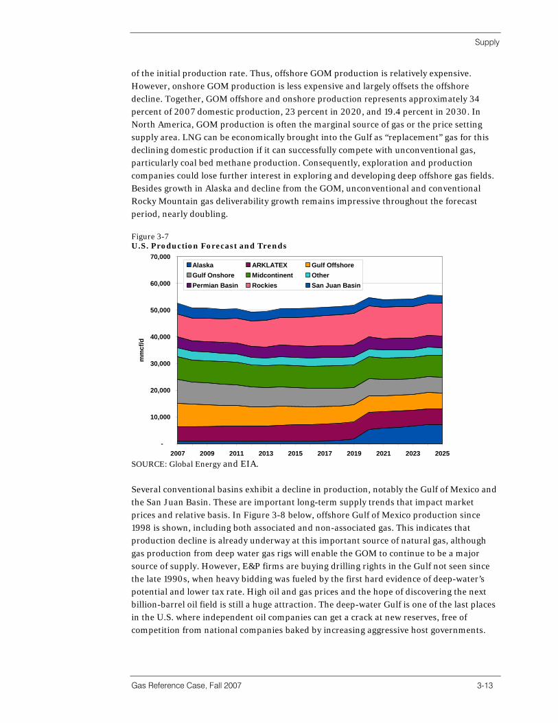
Supply
Gas Reference Case, Fall 2007 3-13
of the initial production rate. Thus, offshore GOM production is relatively expensive. However, onshore GOM production is less expensive and largely offsets the offshore decline. Together, GOM offshore and onshore production represents approximately 34 percent of 2007 domestic production, 23 percent in 2020, and 19.4 percent in 2030. In North America, GOM production is often the marginal source of gas or the price setting supply area. LNG can be economically brought into the Gulf as “replacement” gas for this declining domestic production if it can successfully compete with unconventional gas, particularly coal bed methane production. Consequently, exploration and production companies could lose further interest in exploring and developing deep offshore gas fields. Besides growth in Alaska and decline from the GOM, unconventional and conventional Rocky Mountain gas deliverability growth remains impressive throughout the forecast period, nearly doubling. Figure 3-7 U.S. Production Forecast and Trends
-
10,000
20,000
30,000
40,000
50,000
60,000
70,000
2007 2009 2011 2013 2015 2017 2019 2021 2023 2025
mm
cf/d
Alaska ARKLATEX Gulf OffshoreGulf Onshore Midcontinent OtherPermian Basin Rockies San Juan Basin
SOURCE: Global Energy and EIA. Several conventional basins exhibit a decline in production, notably the Gulf of Mexico and the San Juan Basin. These are important long-term supply trends that impact market prices and relative basis. In Figure 3-8 below, offshore Gulf of Mexico production since 1998 is shown, including both associated and non-associated gas. This indicates that production decline is already underway at this important source of natural gas, although gas production from deep water gas rigs will enable the GOM to continue to be a major source of supply. However, E&P firms are buying drilling rights in the Gulf not seen since the late 1990s, when heavy bidding was fueled by the first hard evidence of deep-water’s potential and lower tax rate. High oil and gas prices and the hope of discovering the next billion-barrel oil field is still a huge attraction. The deep-water Gulf is one of the last places in the U.S. where independent oil companies can get a crack at new reserves, free of competition from national companies baked by increasing aggressive host governments.

Supply
3-14
And new seismic imaging can highlight likely oil and gas reserves though a thick layer of salt beneath the Gulf floor that previously made accurate imaging impossible. Anadarko Petroleum has had some significant success in the deep water, doubling the size of it K2 reservoir to between 2 billion and 4 billion barrels earlier this year.6 Although costs of finding and producing the reserves are several times higher than 10 years ago, the GOM is free of political risk, compared to other parts of the world, and the U.S. government does not require large royalties like other countries, although they were recently raised to 16.7 percent compared to the 12.5 percent for the previous 15 years. Figure 3-8 Long-Term Decline in U.S. Gulf of Mexico Gas Production
0
50
100
150
200
250
300
350
400
450
500
Mar
-98
Jul-9
8
Nov
-98
Mar
-99
Jul-9
9
Nov
-99
Mar
-00
Jul-0
0
Nov
-00
Mar
-01
Jul-0
1
Nov
-01
Mar
-02
Jul-0
2
Nov
-02
Mar
-03
Jul-0
3
Nov
-03
Mar
-04
Jul-0
4
Nov
-04
Mar
-05
Jul-0
5
Nov
-05
Mar
-06
Jul-0
6
Nov
-06
Mar
-07
Jul-0
7
Bcf
/ M
onth
Associated Gas Production from Oil Wells
Gas Production from Gas Wells
Hurricane Katrina (Category 5)
SOURCE: Global Energy and EIA.
Although our expectation is for declining production levels to occur, in the past several years there were many successful new development wells drilled along with many technological milestones. Sub sea production reached depths of greater than 7,500 feet with significant new discoveries in depths greater than 7,000 feet. From 2005 to 2006, 94 new wells were drilled in the deepwater GOM with 36 of them considered ultra-deepwater wells at depths greater than 5,000 feet. Figure 3-9 details the number of working rigs, split between looking for natural gas and crude oil, operating in the GOM since 2000.
6 Wall Street Journal, August 27, 2007
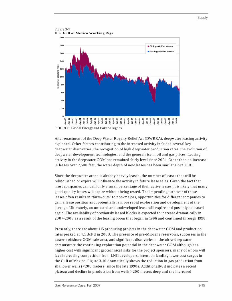
Supply
Gas Reference Case, Fall 2007 3-15
Figure 3-9 U.S. Gulf of Mexico Working Rigs
0
20
40
60
80
100
120
140
160
180
200
Jan-
00
Apr
-00
Jul-0
0
Oct
-00
Jan-
01
Apr
-01
Jul-0
1
Oct
-01
Jan-
02
Apr
-02
Jul-0
2
Oct
-02
Jan-
03
Apr
-03
Jul-0
3
Oct
-03
Jan-
04
Apr
-04
Jul-0
4
Oct
-04
Jan-
05
Apr
-05
Jul-0
5
Oct
-05
Jan-
06
Apr
-06
Jul-0
6
Oct
-06
Jan-
07
Apr
-07
Jul-0
7
Num
ber o
f Wor
king
Rig
s
Oil Rigs-Gulf of Mexico
Gas Rigs-Gulf of Mexico
SOURCE: Global Energy and Baker-Hughes.
After enactment of the Deep Water Royalty Relief Act (DWRRA), deepwater leasing activity exploded. Other factors contributing to the increased activity included several key deepwater discoveries, the recognition of high deepwater production rates, the evolution of deepwater development technologies, and the general rise in oil and gas prices. Leasing activity in the deepwater GOM has remained fairly level since 2001. Other than an increase in leases over 7,500 feet, the water depth of new leases has been similar since 2001. Since the deepwater arena is already heavily leased, the number of leases that will be relinquished or expire will influence the activity in future lease sales. Given the fact that most companies can drill only a small percentage of their active leases, it is likely that many good-quality leases will expire without being tested. The impending turnover of these leases often results in “farm-outs” to non-majors, opportunities for different companies to gain a lease position and, potentially, a more rapid exploration and development of the acreage. Ultimately, an untested and undeveloped lease will expire and possibly be leased again. The availability of previously leased blocks is expected to increase dramatically in 2007-2008 as a result of the leasing boom that began in 1996 and continued through 1998. Presently, there are about 115 producing projects in the deepwater GOM and production rates peaked at 4.1 Bcf/d in 2003. The presence of pre-Miocene reservoirs, successes in the eastern offshore GOM sale area, and significant discoveries in the ultra-deepwater demonstrate the continuing exploration potential in the deepwater GOM although at a higher cost with significant geotechnical risks for the project sponsors, many of whom will face increasing competition from LNG developers, intent on landing lower cost cargos in the Gulf of Mexico. Figure 3-10 dramatically shows the reduction in gas production from shallower wells (<200 meters) since the late 1990s. Additionally, it indicates a recent plateau and decline in production from wells >200 meters deep and the increased
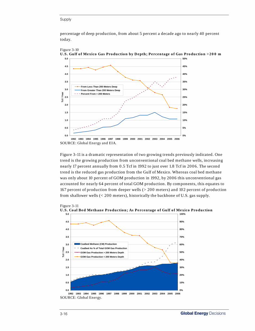
Supply
3-16
percentage of deep production, from about 5 percent a decade ago to nearly 40 percent today. Figure 3-10 U.S. Gulf of Mexico Gas Production by Depth; Percentage of Gas Production >200 m
0.0
0.5
1.0
1.5
2.0
2.5
3.0
3.5
4.0
4.5
5.0
1992 1993 1994 1995 1996 1997 1998 1999 2000 2001 2002 2003 2004 2005 2006
Tcf /
Yea
r
0%
5%
10%
15%
20%
25%
30%
35%
40%
45%
50%
From Less Than 200 Meters DeepFrom Greater Than 200 Meters DeepPercent From > 200 Meters
SOURCE: Global Energy and EIA.
Figure 3-11 is a dramatic representation of two growing trends previously indicated. One trend is the growing production from unconventional coal bed methane wells, increasing nearly 17 percent annually from 0.5 Tcf in 1992 to just over 1.8 Tcf in 2006. The second trend is the reduced gas production from the Gulf of Mexico. Whereas coal bed methane was only about 10 percent of GOM production in 1992, by 2006 this unconventional gas accounted for nearly 64 percent of total GOM production. By components, this equates to 167 percent of production from deeper wells (> 200 meters) and 102 percent of production from shallower wells (< 200 meters), historically the backbone of U.S. gas supply. Figure 3-11 U.S. Coal Bed Methane Production; As Percentage of Gulf of Mexico Production
0.0
0.5
1.0
1.5
2.0
2.5
3.0
3.5
4.0
4.5
5.0
1992 1993 1994 1995 1996 1997 1998 1999 2000 2001 2002 2003 2004 2005 2006
Tcf /
Yea
r
0%
10%
20%
30%
40%
50%
60%
70%
80%
90%
100%
Coalbed Methane (CM) Production
Coalbed As % of Total GOM Gas Production
GOM Gas Production > 200 Meters Depth
GOM Gas Production < 200 Meters Depth
SOURCE: Global Energy.

Supply
Gas Reference Case, Fall 2007 3-17
Working Gas Storage The warm winter of 2005-2006 caused a build up of gas inventories in underground storage and gas prices remained volatile during the summer of 2006, dropping as low as $3.66/dth in September 2006. One reason was much lower storage injections due to high inventories. From February through the end of December 2006, storage inventories achieved record levels mainly in the range of 10-15 percent higher than the five-year maximum. Finally, after a warmer than normal December, much colder than normal weather arrived in late December and inventories fell, and sharply again from January 25 onward as cold weather returned and record gas prices hit the Northeastern and Middle Atlantic states. Citygate prices in the NY/NJ/New England area averaged in the $10 to $15/dth for nearly the next four weeks, with some spot prices as high as $36/dth. Even citygates in Florida reached over $10/dth. Storage withdrawals were maximized since this gas was much cheaper than spot gas, having been injected the prior summer or left over from the summer 2005 injection season. The national storage levels as of early March 2007 stood at 1,526 Bcf, which was 12 percent above the five-year average of 1,358 Bcf for this time of year and is shown in Figure 3-11. This level is under the maximum five-year average of 1,840 Bcf (by about 18 percent), so the extended cold weather throughout much of the United States has left a noticeable dent in the excess storage inventory. However, a relatively cool summer and record volumes of imported LNG conspired to pump up inventories back above the maximum five-year levels, now over 3 Tcf, the highest inventory level ever for late-August or mid-September. Figure 3-12 shows the variations throughout the winter of 2006-2007 as a result of the cold spells along with the gradual inventory gain over the summer of 2007. Figure 3-12 U.S. Annual Storage Activity for Year 2006 through September 1, 2007
500
1000
1500
2000
2500
3000
3500
Jan-06
Feb-06
Mar-06
Apr-06
May-06
Jun-06
Jul-06
Aug-06
Sep-06
Oct-06
Nov-06
Dec-06
Jan-07
Feb-07
Mar-07
Apr-07
May-07
Jun-07
Jul-07
Aug-07
Tota
l Wor
king
Gas
in B
cf
Jan '06 - Aug '075-Year Maximum 5-Year Average5-Year Minimum
Last half of Winter
Late-Spring, Summer and Early-Fall Injection Season
Beginning of Winter
withdrawal season
Late-Spring & Summer Injection Season
SOURCE: Global Energy and EIA.

Supply
3-18
The record cold in January and February also caused a bump up in forward NYMEX gas futures prices for the summer of 2007 since much more injecting will have to be accomplished by the autumn. For example, June and July 2007 forward NYMEX prices increased from around $6.80/dth in late December to the $8.00-$8.20/dth range in late February. Gas inventories fell from about 250 Bcf above the five-year maximum to about 300 Bcf below the five-year maximum. Speculators and hedgers were therefore expecting around 2.5 Bcf/day more injections this summer than last summer when storage levels were at record highs. For several months, the entire summer of 2007 NYMEX was over $8.00/dth, with December through March 2008 prices near $10.00/dth. However, the summer was cooler than last year and coupled with Hurricane Dean missing the offshore gas rigs, prices gradually collapsed over several dollars through late summer. Since that time and as of this writing (mid-September), prices have recovered somewhat. October futures prices are around $5.90/dth and January/February 2008 prices about $7.90/dth. Much of the reason for the nearly $2/dth drop in summer prices is due to high storage levels and record volumes of LNG being imported into the United States. The second quarter of 2007 set a record for import volumes. But the normal volatility of natural gas, coupled with the recent rise in WTI crude prices, mean that daily swings in NYMEX gas of +/- $0.30/dth are common.
Market Hubs Essential to supply management are market hubs. The natural gas industry has undergone major changes over the past two decades. It has evolved from being highly regulated in both the upstream and downstream sectors to a highly tradable, deregulated commodity. With the unbundling of pipeline transportation services and open access being established, the number of market participants has multiplied, as have the number of markets at which gas can be exchanged on a spot or forward basis. These markets, called hubs, are found at the interconnections of major interstate and intrastate pipelines and often where gas storage is available. Many times short-term “park and loan” arrangements can be made between parties with negotiable daily rates. Below is a comprehensive list of the main services: • Parking: short-term holding of a shipper’s gas prior to redelivery; • Loaning: short-term gas advance to a shipper repaid at a later date; • Wheeling: transfer from one pipeline to another; • Storage: longer than loaning; includes injection and withdrawal; • Balancing: short-term interruptible action to cover temporary imbalance; • Peaking: very short-term (typically less than a day and even hourly) sales; • Title Transfer: services where changes in ownership are recording, such as one
company’s positive imbalance with another company’s negative imbalance in order to avoid penalties; and
• Electronic Trading: trading system electronically or through negotiation matching buyer and seller.
The first natural gas hub to come into existence was the Henry Hub in 1988 at Erath, Louisiana, and remains the largest and most active market in the continental natural gas market. It is a critical junction for much of the rich Gulf of Mexico production areas. This is
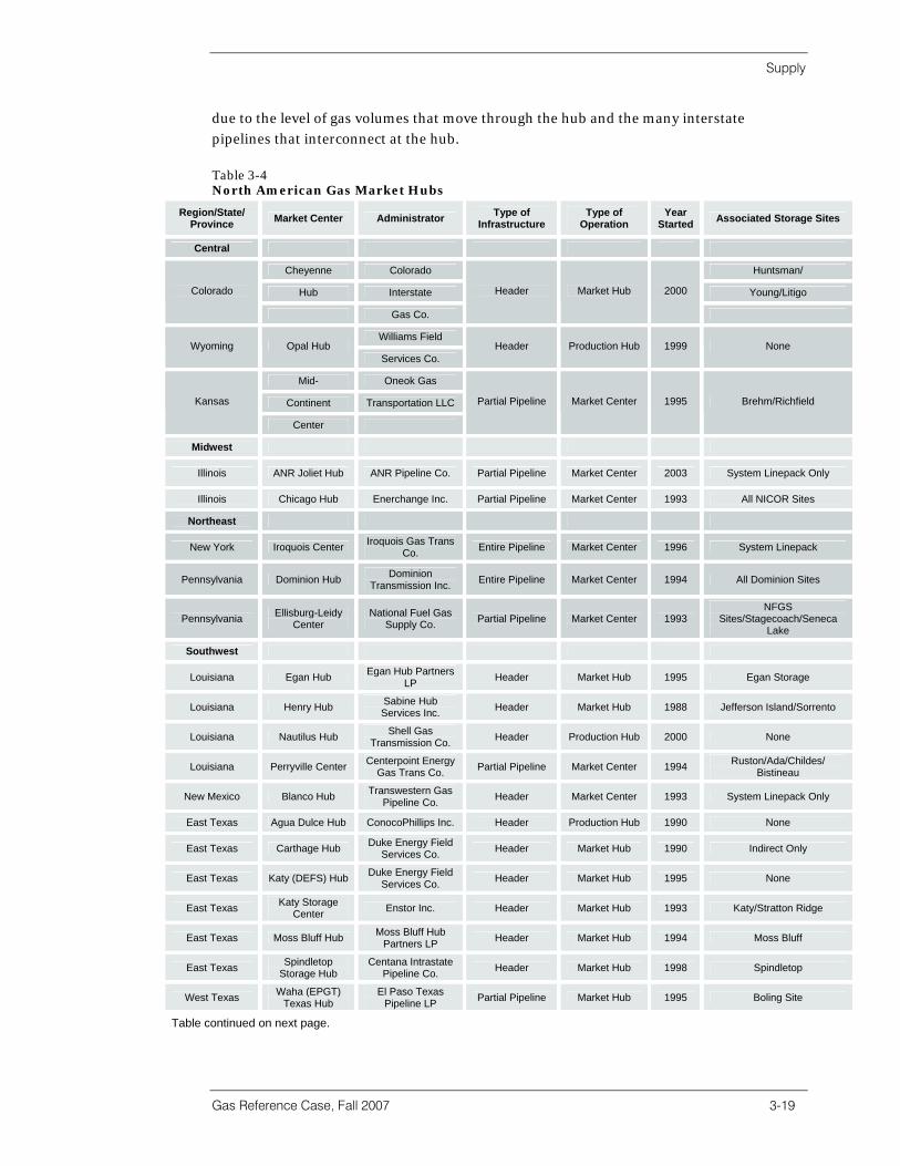
Supply
Gas Reference Case, Fall 2007 3-19
due to the level of gas volumes that move through the hub and the many interstate pipelines that interconnect at the hub. Table 3-4 North American Gas Market Hubs
Region/State/ Province Market Center Administrator Type of
Infrastructure Type of
Operation Year
Started Associated Storage Sites
Central
Cheyenne Colorado Huntsman/
Hub Interstate Young/Litigo Colorado
Gas Co.
Header Market Hub 2000
Williams Field Wyoming Opal Hub
Services Co. Header Production Hub 1999 None
Mid- Oneok Gas
Continent Transportation LLC Kansas
Center
Partial Pipeline Market Center 1995 Brehm/Richfield
Midwest
Illinois ANR Joliet Hub ANR Pipeline Co. Partial Pipeline Market Center 2003 System Linepack Only
Illinois Chicago Hub Enerchange Inc. Partial Pipeline Market Center 1993 All NICOR Sites
Northeast
New York Iroquois Center Iroquois Gas Trans Co. Entire Pipeline Market Center 1996 System Linepack
Pennsylvania Dominion Hub Dominion Transmission Inc. Entire Pipeline Market Center 1994 All Dominion Sites
Pennsylvania Ellisburg-Leidy Center
National Fuel Gas Supply Co. Partial Pipeline Market Center 1993
NFGS Sites/Stagecoach/Seneca
Lake
Southwest
Louisiana Egan Hub Egan Hub Partners LP Header Market Hub 1995 Egan Storage
Louisiana Henry Hub Sabine Hub Services Inc. Header Market Hub 1988 Jefferson Island/Sorrento
Louisiana Nautilus Hub Shell Gas Transmission Co. Header Production Hub 2000 None
Louisiana Perryville Center Centerpoint Energy Gas Trans Co. Partial Pipeline Market Center 1994 Ruston/Ada/Childes/
Bistineau
New Mexico Blanco Hub Transwestern Gas Pipeline Co. Header Market Center 1993 System Linepack Only
East Texas Agua Dulce Hub ConocoPhillips Inc. Header Production Hub 1990 None
East Texas Carthage Hub Duke Energy Field Services Co. Header Market Hub 1990 Indirect Only
East Texas Katy (DEFS) Hub Duke Energy Field Services Co. Header Market Hub 1995 None
East Texas Katy Storage Center Enstor Inc. Header Market Hub 1993 Katy/Stratton Ridge
East Texas Moss Bluff Hub Moss Bluff Hub Partners LP Header Market Hub 1994 Moss Bluff
East Texas Spindletop Storage Hub
Centana Intrastate Pipeline Co. Header Market Hub 1998 Spindletop
West Texas Waha (EPGT) Texas Hub
El Paso Texas Pipeline LP Partial Pipeline Market Hub 1995 Boling Site
Table continued on next page.

Supply
3-20
Region/State/ Province Market Center Administrator Type of
Infrastructure Type of
Operation Year
Started Associated Storage Sites
West Texas Waha (DEFS) Hub
Duke Energy Field Service Co. Header Market Hub 1995 None
West Texas Waha (Encina) Hub
Sid Richardson Gas Co. Partial Pipeline Production Hub 1995 None
West Texas Waha (Lone Star) Hub
TXU Lone Star Gas Co. Header Market Hub 1995 Keystone
Western
California California Energy Hub
Southern California Gas Co. Partial Pipeline Market Center 1994 All SoCal Fields
California Golden Gate Center
Pacific Gas & Electric Co. Entire Pipeline Market Center 1996 All PG&E Fields & Linepack
Idaho Kingsgate Center PG&E Gas Transmission - NW Partial Pipeline Market Hub
Services 1994 System Linepack Only
Oregon Malin Center PG&E Gas Transmission - NW Partial Pipeline Market Hub
Service 1994 System Linepack Only
Oregon Stanfield Center Pacific Gas Transmission Co. Partial Pipeline Market Hub
Services 1994 System Linepack Only
Canada
Alberta AECO-C Hub EnCana Energy Co. Partial Pipeline Market Center 1990 Suffield/Dunvegan/Carbon
Alberta Alberta Hub Enstor - PPM Energy Inc. Header Market Hub 1997 Alberta Hub
Alberta Alberta Market Center
Atco Gas Services Ltd. Header Market Hub 1998 Carbon Facility
Alberta Crossfield Hub Crossalta Gas Storage & Services Header Market Hub 1995 East Crossfield
Alberta Empress Center Transcanada Gas Pipeline Ltd. Header Market Hub 1986 Linepack
Alberta Intra-Alberta Center
Transcanada Gas Pipelines Ltd. Entire Pipeline Market Center 1994 Indirect Only
British Columbia Sumas Center Westcoast Pipeline Co. Partial Pipeline Market Hub 1994 Aitken Creek
Alberta=>Québec TransCanada Center
Transcanada Gas Pipelines Ltd. Entire Pipeline Market Hub 1998 Indirect Only
Ontario Dawn Market Center Union Gas Ltd. Entire Pipeline Market Hub 1985 Dawn (20 fields)
SOURCE: EIA, Office of Oil and Gas, Natural Gas Division; Pipeline & Gas Journal.
Henry Hub is also the pricing point for the New York Mercantile Exchange (NYMEX) natural gas futures contract. The current NYMEX futures contract is highly liquid. In fact, in terms of relative contract liquidity, the Henry Hub futures market ranks ahead of many other commodities and even some international currencies. Henry Hub is probably the most ideal gas hub in North America because it has interconnections with a dozen large diameter pipeline systems (eight interstate and four intrastate), two large gas gathering systems (one offshore and one onshore), and two storage systems as well as being located near all three major types of reservoirs used for natural gas storage: salt dome, aquifer, and depleted fields. Each storage reservoir has very specific operating and cycling parameters that depend on the reservoir geology of the structure and on installed compression capacity. Salt reservoirs have the highest deliverability and multi-cycling capacity, but the majority of working natural gas storage resides in depleted oil and gas reservoirs. Henry Hub might even eventually be connected to an LNG terminal.
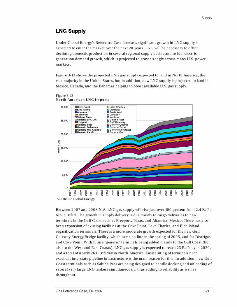
Supply
Gas Reference Case, Fall 2007 3-21
LNG Supply Under Global Energy’s Reference Case forecast, significant growth in LNG supply is expected to enter the market over the next 20 years. LNG will be necessary to offset declining domestic production in several regional supply basins and to fuel electric generation demand growth, which is projected to grow strongly across many U.S. power markets. Figure 3-13 shows the projected LNG gas supply expected to land in North America, the vast majority in the United States, but in addition, new LNG supply is projected to land in Mexico, Canada, and the Bahamas helping to boost available U.S. gas supply. Figure 3-13 North American LNG Imports
0
5,000
10,000
15,000
20,000
25,000
30,000
2007
2008
2009
2010
2011
2012
2013
2014
2015
2016
2017
2018
2019
2020
2021
2022
2023
2024
2025
2026
2027
2028
2029
2030
MM
cf /
Day
Cove Point Lake CharlesElba Island DistrigasAltamira Costa AzulCameron CanaportSabine Pass NeptuneGeneric Brit. Col. Golden PassFreeport Gulf GatewayGeneric Baja Generic QuebecGeneric Bahamas Generic TexasGeneric Mid-Atlantic Generic NortheastGeneric Pacific Generic Gulf
SOURCE: Global Energy.
Between 2007 and 2008 N.A. LNG gas supply will rise just over 100 percent from 2.4 Bcf/d to 5.3 Bcf/d. The growth in supply delivery is due mostly to cargo deliveries to new terminals in the Gulf Coast such as Freeport, Texas, and Altamira, Mexico. There has also been expansion of existing facilities at the Cove Point, Lake Charles, and Elba Island regasification terminals. There is a more moderate growth expected for the new Gulf Gateway Energy Bridge facility, which came on line in the spring of 2005, and for Distrigas and Cove Point. With future “generic” terminals being added mainly to the Gulf Coast (but also to the West and East Coasts), LNG gas supply is expected to reach 23 Bcf/day in 2030, and a total of nearly 26.6 Bcf/day in North America. Easier siting of terminals near excellent interstate pipeline infrastructure is the main reason for this. In addition, new Gulf Coast terminals such as Sabine Pass are being designed to handle docking and unloading of several very large LNG tankers simultaneously, thus adding to reliability as well as throughput.
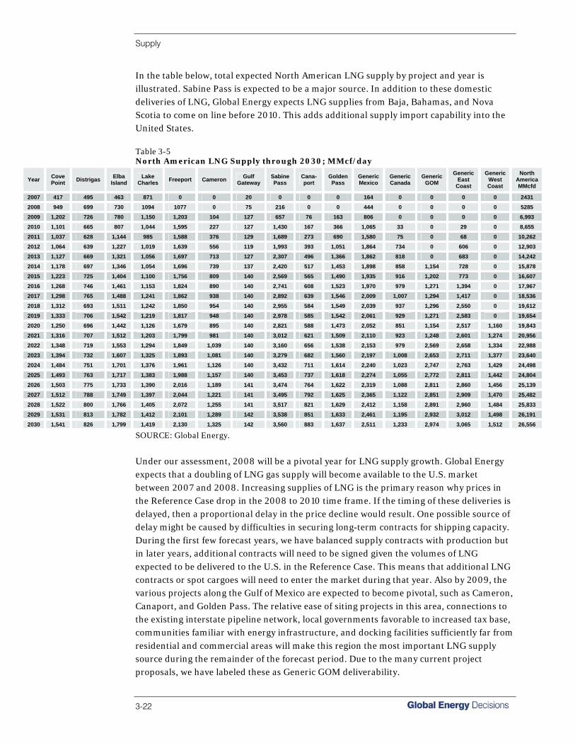
Supply
3-22
In the table below, total expected North American LNG supply by project and year is illustrated. Sabine Pass is expected to be a major source. In addition to these domestic deliveries of LNG, Global Energy expects LNG supplies from Baja, Bahamas, and Nova Scotia to come on line before 2010. This adds additional supply import capability into the United States. Table 3-5 North American LNG Supply through 2030; MMcf/day
Year Cove Point Distrigas Elba
Island Lake
Charles Freeport Cameron Gulf Gateway
Sabine Pass
Cana-port
Golden Pass
Generic Mexico
Generic Canada
Generic GOM
Generic East
Coast
Generic West Coast
North America MMcfd
2007 417 495 463 871 0 0 20 0 0 0 164 0 0 0 0 2431
2008 949 699 730 1094 1077 0 75 216 0 0 444 0 0 0 0 5285
2009 1,202 726 780 1,150 1,203 104 127 657 76 163 806 0 0 0 0 6,993
2010 1,101 665 807 1,044 1,595 227 127 1,430 167 366 1,065 33 0 29 0 8,655
2011 1,037 628 1,144 985 1,588 376 129 1,689 273 690 1,580 75 0 68 0 10,262
2012 1,064 639 1,227 1,019 1,639 556 119 1,993 393 1,051 1,864 734 0 606 0 12,903
2013 1,127 669 1,321 1,056 1,697 713 127 2,307 496 1,366 1,862 818 0 683 0 14,242
2014 1,178 697 1,346 1,054 1,696 739 137 2,420 517 1,453 1,898 858 1,154 728 0 15,878
2015 1,223 725 1,404 1,100 1,756 809 140 2,569 565 1,490 1,935 916 1,202 773 0 16,607
2016 1,268 746 1,461 1,153 1,824 890 140 2,741 608 1,523 1,970 979 1,271 1,394 0 17,967
2017 1,298 765 1,488 1,241 1,862 938 140 2,892 639 1,546 2,009 1,007 1,294 1,417 0 18,536
2018 1,312 693 1,511 1,242 1,850 954 140 2,955 584 1,549 2,039 937 1,296 2,550 0 19,612
2019 1,333 706 1,542 1,219 1,817 948 140 2,978 585 1,542 2,061 929 1,271 2,583 0 19,654
2020 1,250 696 1,442 1,126 1,679 895 140 2,821 588 1,473 2,052 851 1,154 2,517 1,160 19,843
2021 1,316 707 1,512 1,203 1,799 981 140 3,012 621 1,509 2,110 923 1,248 2,601 1,274 20,956
2022 1,348 719 1,553 1,294 1,849 1,039 140 3,160 656 1,538 2,153 979 2,569 2,658 1,334 22,988
2023 1,394 732 1,607 1,325 1,893 1,081 140 3,279 682 1,560 2,197 1,008 2,653 2,711 1,377 23,640
2024 1,484 751 1,701 1,376 1,961 1,126 140 3,432 711 1,614 2,240 1,023 2,747 2,763 1,429 24,498
2025 1,493 763 1,717 1,383 1,988 1,157 140 3,453 737 1,618 2,274 1,055 2,772 2,811 1,442 24,804
2026 1,503 775 1,733 1,390 2,016 1,189 141 3,474 764 1,622 2,319 1,088 2,811 2,860 1,456 25,139
2027 1,512 788 1,749 1,397 2,044 1,221 141 3,495 792 1,625 2,365 1,122 2,851 2,909 1,470 25,482
2028 1,522 800 1,766 1,405 2,072 1,255 141 3,517 821 1,629 2,412 1,158 2,891 2,960 1,484 25,833
2029 1,531 813 1,782 1,412 2,101 1,289 142 3,538 851 1,633 2,461 1,195 2,932 3,012 1,498 26,191
2030 1,541 826 1,799 1,419 2,130 1,325 142 3,560 883 1,637 2,511 1,233 2,974 3,065 1,512 26,556
SOURCE: Global Energy.
Under our assessment, 2008 will be a pivotal year for LNG supply growth. Global Energy expects that a doubling of LNG gas supply will become available to the U.S. market between 2007 and 2008. Increasing supplies of LNG is the primary reason why prices in the Reference Case drop in the 2008 to 2010 time frame. If the timing of these deliveries is delayed, then a proportional delay in the price decline would result. One possible source of delay might be caused by difficulties in securing long-term contracts for shipping capacity. During the first few forecast years, we have balanced supply contracts with production but in later years, additional contracts will need to be signed given the volumes of LNG expected to be delivered to the U.S. in the Reference Case. This means that additional LNG contracts or spot cargoes will need to enter the market during that year. Also by 2009, the various projects along the Gulf of Mexico are expected to become pivotal, such as Cameron, Canaport, and Golden Pass. The relative ease of siting projects in this area, connections to the existing interstate pipeline network, local governments favorable to increased tax base, communities familiar with energy infrastructure, and docking facilities sufficiently far from residential and commercial areas will make this region the most important LNG supply source during the remainder of the forecast period. Due to the many current project proposals, we have labeled these as Generic GOM deliverability.

Supply
Gas Reference Case, Fall 2007 3-23
Supply Uncertainty In the tables and figures above, Global Energy has presented its Reference Case assessment of future natural gas supply sources available to satisfy U.S. gas demand through 2025. We believe the sources and methodologies used to prepare these assessments are reliable, use reasonable assumptions, and are based on reasonable judgment. However, forecasting gas supply from unproved resources or uncompleted LNG supply-chain facilities is inherently uncertain, much more so than would be the case for projecting electric power plant development or many other industrial development activities. New exploration concepts are constantly being developed and discarded as petroleum geologists, geophysicists, and engineers re-evaluate new data. The development and application of new technologies, which tends to be unevenly distributed in time, can materially lower supply costs. The cost of materials such as steel and chemicals used in production also are difficult to forecast many years into the future due to the complex and competitive global trading of these manufactured products. The growing reliance on unconventional gas sources such as coal bed methane, tight gas, and shales also requires projection of full-cycle recovery costs with a range of uncertainties, particularly on production decline rates and on water treatment and disposal costs. Actual costs incurred may not reflect these projections. Restrictions on access to and use of land for exploration and development, especially for unconventional reserves, will also materially affect supply recovery cost, and over the 20-year time frame considered, could materially impact supply availability and price forecast results. For example, in the Reference Case, we have assumed no lifting of restrictions on exploration and development in the North Slope of Alaska or the eastern Gulf of Mexico. Either of these regions alone likely holds significant hydrocarbon reserves, which for the time being are off limits to exploration and development. Restrictions preventing drilling in other gas-resource rich regions include both the Atlantic and Pacific coasts. Another source of uncertainty centers on pipeline rights of way and stable fiscal policy. In particular, aboriginal land holders in Northern Canada could hold up northern pipeline development from both Alaska and the Mackenzie Valley where proved reserves total approximately 40 Tcf. In Alaska, conversion of state gas royalty and tax burdens into working-interest gas is under current analysis by various state departments and the state legislature. In addition, potential governmental cost and price support mechanisms for commercialization of this stranded associated-gas have been repeatedly debated among the state, federal government, and other stakeholders. Such debate may delay our projection of the economic development of such gas. Given the size of these northern projects, up to 6.5 Bcf/d for Alaska and up to 2.4 Bcf/d from northern Canada, extended delays will also materially impact Global Energy’s forecast of supply availability and market prices. The final source of uncertainty is centered on LNG supply. Greater volumes of LNG sourced from beyond North America introduces another level of supply and price risk, which is projected to increase as U.S. reliance on LNG imports increases from about 2.4
Supply
3-24
percent of demand in 2006 at a regasification capacity utilization rate of 31 percent, to over 32 percent of demand by 2025 at a utilization rate of over 60 percent. What type of market environment will develop? Will some form of supply cartel evolve and will oligopolistic market prices be established? In our Reference Case analysis, we assume the LNG suppliers will be price takers, and that LNG will establish a floor price compared to indigenous gas. This is a reasonable assumption given the cost advantage these producers have relative to many North American supply regions, particularly on a marginal cost basis for incremental supply. However, LNG suppliers could tacitly or overtly act to provide surplus supply and use LNG as a ceiling price or cap compared to indigenous gas, thereby establishing LNG as a price maker to capture market share rather than maximize net-back pricing. This potential control of volume and price will materially affect our long-term price forecast based on supply and demand fundamentals, particularly if LNG pricing is tied to the short-term and volatile NYMEX, compared to a cost-of-service structure with an embedded risk-weighted, globally competitive return on equity for the supply segments upstream of the regasification terminals.

Section 4 | Liquefied Natural Gas (LNG)


Liquefied Natural Gas (LNG)
Gas Reference Case, Fall 2007 4-1
Introduction With natural gas prices remaining at stubbornly high levels and domestic production stagnating in the face of projected U.S. demand growth coupled with reduced Canadian imports, the need for additional sources of gas has become very apparent. In fact, even Alan Greenspan, the former chairman of the Federal Reserve has weighed in on the debate. The 2005 hurricanes and resulting damage to Gulf of Mexico production pushed prices up even further. There are still some minor amounts of natural gas production in the Gulf of Mexico off line due to the unprecedented level of damage. Historically, virtually all natural gas consumed in the United States has been sourced from indigenous Lower 48 production and pipeline imports from Canada. Mexico, although it has significant natural gas resource potential, has tended to be a net importer of natural gas from the United States and is expected to continue. For most of its history, the continental natural gas trade has existed largely without a global influence affecting market prices. Going forward, it is likely that the North American gas market and elsewhere will be increasingly influenced by the development of a global natural gas trade involving LNG and its competitive position with long-haul, cross-border pipeline gas and alternative fuel oils. In 2006, the United States consumed about 22 Tcf of natural gas while domestic dry gas production was estimated to be 18.5 Tcf. As Figure 4-1 indicates, the balance of gas consumed was met by imports, primarily from Canada via pipeline (15.9 percent, 3.5 Tcf) and in the form of LNG (2.6 percent, 0.53 Tcf). Figure 4-1 U.S. Supply Allocation in 2006
US Dry Gas Production
81.6%
Net Pipeline Imports15.9%
LNG Imports2.6%
Note: Excludes Alaska LNG exports. SOURCE: EIA.
Over the forecast horizon, we expect that natural gas consumption in the United States will grow at an annual average rate of nearly 2 percent. Despite the expected demand increase, natural gas production—conventional and unconventional—from the United States and Canada are not anticipated to meet much of the incremental demand growth.

Liquefied Natural Gas (LNG)
4-2
A myriad of factors is contributing to our net overall stagnant production outlook. Paramount among these factors is: • Increased Exploration and Production (E&P) Costs - Our research indicates the E&P
costs for conventional reserves in the United States have increased by as much as 70 percent since 2000 in some regions. Although we view the large increase as partially transitory, we are modeling a trend of increased costs over the forecast horizon. This is reflected in rising market prices in the later half of the forecast. Conventional supply costs appear to be increasing at a rate that is not being significantly offset by new technologies. A major driver of this phenomenon is that available resources seem to be decreasing in quality, thus increasing the cost of finding and development on a per unit basis. Ultimately, there appears to be less economic incentive for the integrated multinational majors to invest significantly in new North American natural gas production outside of the Arctic, the deepwater Gulf of Mexico (GOM), and the ultra-deep GOM shelf.
• Access Limitations - Although a significant resource potential exists in many regions of the United States (the Pacific Offshore, the Rockies, the eastern Gulf of Mexico, and the Atlantic Offshore), prevailing restrictive legislation and infrastructure limitations will play down any significant contribution from these resources over the forecast horizon.
• Unconventional reservoirs of non-associated gas will largely balance the decline in conventional production capacity and are the main competitor, particularly coal-bed methane in the Rocky Mountain region, of imported LNG for incremental supply.
The recent high commodity price environment has allowed for increased drilling activity in the United States and Canada over the past several years. In fact the number of active drill rigs targeting gas recently exceeded 1,780. However, the increase in gas directed rigs has simply made up for production declines in the maturing reserve base, rather than fostering year over year growth in production capacity. From 2000 to 2006, U.S. dry production declined by about 0.7 Tcf, an average of 0.6 percent per year while the number of active rigs increased about 100 percent from 770 in 2000 to an average of over 1,500 in 2006. However, U.S. proved gas reserves have been on the rise with more favorable market prices. What is certain is that the polices that promoted natural gas as the fuel of choice for gas-fired generation and the likely corresponding increase in natural gas demand will need to be aligned with a balanced approach to ensure supply adequacy. The potential supply dilemma facing the United States can be averted by realizing further energy efficiency gains, employing a more balanced approach to future generation resource planning (including the use of more fuel-switching capacity and of emission credits), deliveries of Arctic supplies, and the timely development of liquefied natural gas (LNG). LNG is the one solution currently being developed that can accommodate expected market growth over the forecast horizon. LNG is an attractive alternative due to the relative abundance of gas resources globally. Further, LNG has become increasingly
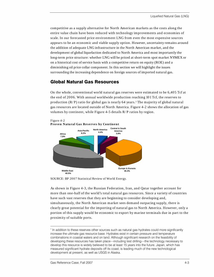
Liquefied Natural Gas (LNG)
Gas Reference Case, Fall 2007 4-3
competitive as a supply alternative for North American markets as the costs along the entire value chain have been reduced with technology improvements and economies of scale. In our forecasted price environment LNG from even the most expensive sources appears to be an economic and viable supply option. However, uncertainty remains around the addition of adequate LNG infrastructure in the North American market, and the development of global liquefaction dedicated to North America and most importantly the long-term price structure: whether LNG will be priced at short-term spot market NYMEX or on a historical cost of service basis with a competitive return on equity (ROE) and a diminishing oil price collar component. In this section we will highlight the issues surrounding the increasing dependence on foreign sources of imported natural gas.
Global Natural Gas Resources On the whole, conventional world natural gas reserves were estimated to be 6,405 Tcf at the end of 2006. With annual worldwide production reaching 101 Tcf, the reserves to production (R/P) ratio for global gas is nearly 64 years.1 The majority of global natural gas resources are located outside of North America. Figure 4-2 shows the allocation of gas volumes by continent, while Figure 4-5 details R/P ratios by region. Figure 4-2 Proven Natural Gas Reserves by Continent
Central & South America
3.8%
Europe & Eurasia35.3%
Asia-Pacific8.2%
North America 4.4%
Africa7.8%
Middle East 40.5%
SOURCE: BP 2007 Statistical Review of World Energy.
As shown in Figure 4-3, the Russian Federation, Iran, and Qatar together account for more than one-half of the world’s total natural gas resources. Since a variety of countries have such vast reserves that they are beginning to consider developing and, simultaneously, the North American market sees demand outpacing supply, there is clearly great potential for the importing of natural gas to North America. However, only a portion of this supply would be economic to export by marine terminals due in part to the proximity of suitable ports.
1 In addition to these reserves other sources such as natural gas hydrates could more significantly increase the ultimate gas resource base. Hydrates exist in certain pressure and temperature combinations in coastal waters and on land. Although significant research on the feasibility of developing these resources has taken place—including test drilling—the technology necessary to develop this resource is widely believed to be at least 15 years into the future. Japan, which has measured significant hydrate deposits off its coast, is leading much of the new technological development at present, as well as USGS in Alaska.
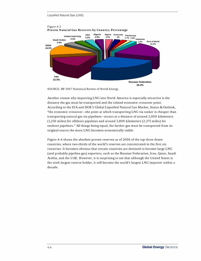
Liquefied Natural Gas (LNG)
4-4
Figure 4-3 Proven Natural Gas Reserves by Country; Percentage
Qatar14.0%
Iran15.5%
Russian Federation26.3%
Norway1.6% Indonesia
1.5%
Iraq1.7%
Venezuela2%
Saudi Arabia3.9%
United Arab Emp.3.3%
Rest of World21.2%
Nigeria2.9%
USA3.3%
Algeria2.5%
SOURCE: BP 2007 Statistical Review of World Energy.
Another reason why importing LNG into North America is especially attractive is the distance the gas must be transported and the related economic crossover point. According to the EIA and DOE’s Global Liquefied Natural Gas Market, Status & Outlook, “the economic crossover—the point at which transporting LNG via tanker is cheaper than transporting natural gas via pipelines—occurs at a distance of around 2,000 kilometers (1,250 miles) for offshore pipelines and around 3,800 kilometers (2,375 miles) for onshore pipelines.” All things being equal, the farther gas must be transported from its original source the more LNG becomes economically viable. Figure 4-4 shows the absolute proven reserves as of 2006 of the top three dozen countries, where two-thirds of the world’s reserves are concentrated in the first six countries. It becomes obvious that certain countries are destined to become large LNG (and probably pipeline gas) exporters, such as the Russian Federation, Iran, Qatar, Saudi Arabia, and the UAE. However, it is surprising to see that although the United States is the sixth largest reserve holder, it will become the world’s largest LNG importer within a decade.
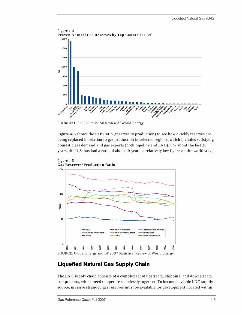
Liquefied Natural Gas (LNG)
Gas Reference Case, Fall 2007 4-5
Figure 4-4 Proven Natural Gas Reserves by Top Countries; Tcf
0
250
500
750
1000
1250
1500
1750
Russia
n Fed
.Ira
nQata
r
Saud
i Ara
bia
United
Ara
b Emp.
USA
Niger
ia
Alger
ia
Vene
zuela Ira
q
Norway
Indon
esia
Austra
lia
Malays
ia
ChinaEg
ypt
Kuwait
Canad
a
Nethe
rland
s
Liby
aIndia
Oman
Pakis
tan
Bolivia
Roman
ia
Myanm
ar
Trinida
d&To
bago
United
King
dom
Bangla
desh
Argen
tina
Mexico
Brazil
Peru
Brune
i
Thail
and
Syria
Tcf
SOURCE: BP 2007 Statistical Review of World Energy. Figure 4-5 shows the R/P Ratio (reserves to production) to see how quickly reserves are being replaced in relation to gas production in selected regions, which includes satisfying domestic gas demand and gas exports (both pipeline and LNG). For about the last 20 years, the U.S. has had a ratio of about 10 years, a relatively low figure on the world stage. Figure 4-5 Gas Reserves/Production Ratio
1
10
100
1000
1980
1982
1984
1986
1988
1990
1992
1994
1996
1998
2000
2002
2004
2006
Year
s
USA Other N.America Central/South AmericaRussian Federation Other Europe/Eurasia Middle EastAfrica China Other Asia/Pacific
SOURCE: Global Energy and BP 2007 Statistical Review of World Energy.
Liquefied Natural Gas Supply Chain The LNG supply chain consists of a complex set of upstream, shipping, and downstream components, which need to operate seamlessly together. To become a viable LNG supply source, massive stranded gas reserves must be available for development, located within

Liquefied Natural Gas (LNG)
4-6
relatively close proximity of a deepwater harbor, and have little if any opportunity cost. These reserves need to be stranded and large enough to support LNG production from one or more liquefaction trains capable of producing anywhere from 3 to 8 million tonnes per year each. Depending upon liquids content, one tonne is roughly equivalent to about 51 MMBtu.2 This represents the amount of gross LNG prior to shrinkage and supply industry usage to transport and deliver pipeline quality gas downstream. In general, about 10 percent of the LNG is consumed prior to pipeline delivery. LNG Liquefaction
Liquefaction is the process of converting natural gas to a liquid by cooling gaseous natural gas to a temperature below -260°F at atmospheric pressure. The process of liquefaction reduces the volume of natural gas by a factor of 610. While in a liquid state, natural gas can be loaded onto tankers that are designed specifically for shipping liquefied natural gas. These tankers can move cryogenic natural gas over long distances, which allows for global trade. Once an LNG cargo reaches its destination, the gas is warmed through the process of regasification and prepared for entry into a natural gas transmission grid. Oftentimes, regasified LNG does not meet local gas quality specifications. The most important issue surrounding regasified LNG quality is that the heat content of cargoes varies significantly depending on the origin of the LNG. Therefore, additional processing such as nitrogen blending or liquids stripping is required before regasified LNG can be introduced into the local pipeline grid. The total amount of upstream gas required to deliver one unit of regasified LNG is approximately 35 percent. In addition, financing usually requires a 20-year proved reserve margin of 40 percent more reserves than required for market delivery. LNG Transportation
Once natural gas is liquefied, it is loaded onto an LNG tanker. LNG tankers are designed with double hulls to prevent accidents and to insulate the cryogenic cargo. LNG is stored in either a prismatic free standing tank, a spherical tank, or a membrane tank. Due to the cryogenic nature of the cargo, the tanks must be constructed with material able to withstand very low temperatures such as stainless steel, aluminum, or invar (invar was the first successful attempt at making a metal alloy that exhibits a nearly zero coefficient of thermal expansion). Presently, large modern tankers generally carry about 138,000 cubic meters of LNG (equivalent to 2.9 Bcf of natural gas) and cost about $180 million, although ships with larger capacities—over 200,000 cubic meters—are being proposed. During shipping some of the LNG cargo is lost to boil-off. Boil-off generally occurs at a rate of about 0.15 percent of the cargo per day. Round-trip shipping time to the United States ranges from 11-14 days (Caribbean supply) to 19-32 days (African supply) to 42-50 days (Persian Gulf). Some tankers, like the Excelsior, the first of Excelerate’s fleet of Energy Bridge Regasification Vessels, which are being used at the Gulf Gateway Energy Bridge in the Gulf of Mexico, have onboard regasification technology. However, most tankers rely on marine import terminals for regasification of their cargo.
2 One tonne or metric ton is equal to 1,000 Kg or about 2,200 lbs.
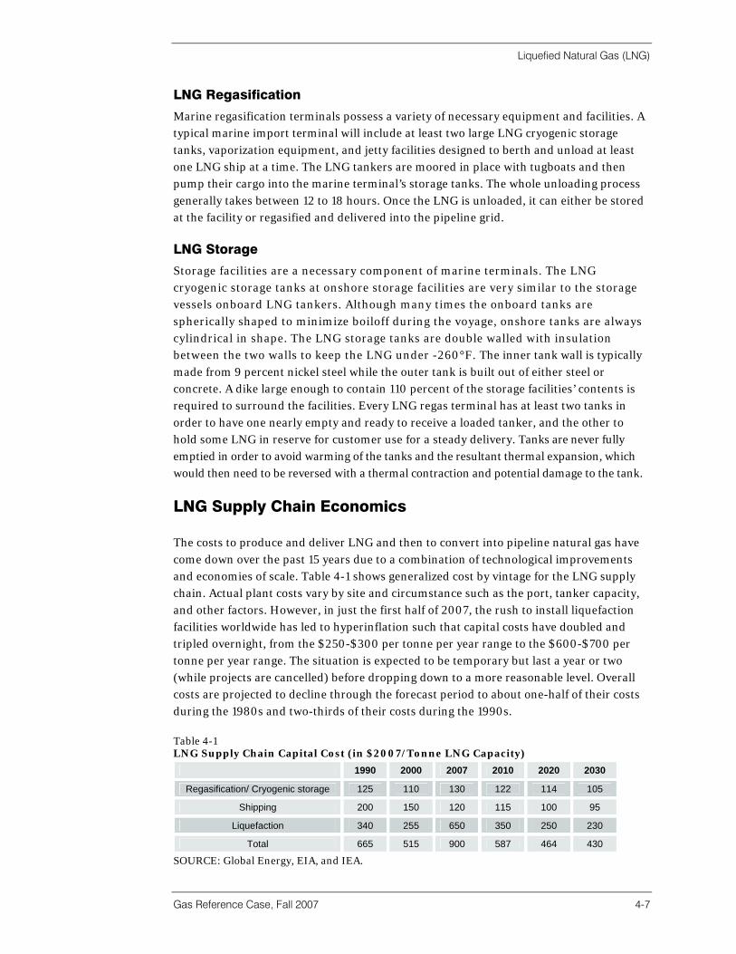
Liquefied Natural Gas (LNG)
Gas Reference Case, Fall 2007 4-7
LNG Regasification
Marine regasification terminals possess a variety of necessary equipment and facilities. A typical marine import terminal will include at least two large LNG cryogenic storage tanks, vaporization equipment, and jetty facilities designed to berth and unload at least one LNG ship at a time. The LNG tankers are moored in place with tugboats and then pump their cargo into the marine terminal’s storage tanks. The whole unloading process generally takes between 12 to 18 hours. Once the LNG is unloaded, it can either be stored at the facility or regasified and delivered into the pipeline grid. LNG Storage
Storage facilities are a necessary component of marine terminals. The LNG cryogenic storage tanks at onshore storage facilities are very similar to the storage vessels onboard LNG tankers. Although many times the onboard tanks are spherically shaped to minimize boiloff during the voyage, onshore tanks are always cylindrical in shape. The LNG storage tanks are double walled with insulation between the two walls to keep the LNG under -260°F. The inner tank wall is typically made from 9 percent nickel steel while the outer tank is built out of either steel or concrete. A dike large enough to contain 110 percent of the storage facilities’ contents is required to surround the facilities. Every LNG regas terminal has at least two tanks in order to have one nearly empty and ready to receive a loaded tanker, and the other to hold some LNG in reserve for customer use for a steady delivery. Tanks are never fully emptied in order to avoid warming of the tanks and the resultant thermal expansion, which would then need to be reversed with a thermal contraction and potential damage to the tank.
LNG Supply Chain Economics The costs to produce and deliver LNG and then to convert into pipeline natural gas have come down over the past 15 years due to a combination of technological improvements and economies of scale. Table 4-1 shows generalized cost by vintage for the LNG supply chain. Actual plant costs vary by site and circumstance such as the port, tanker capacity, and other factors. However, in just the first half of 2007, the rush to install liquefaction facilities worldwide has led to hyperinflation such that capital costs have doubled and tripled overnight, from the $250-$300 per tonne per year range to the $600-$700 per tonne per year range. The situation is expected to be temporary but last a year or two (while projects are cancelled) before dropping down to a more reasonable level. Overall costs are projected to decline through the forecast period to about one-half of their costs during the 1980s and two-thirds of their costs during the 1990s. Table 4-1 LNG Supply Chain Capital Cost (in $2007/Tonne LNG Capacity)
1990 2000 2007 2010 2020 2030
Regasification/ Cryogenic storage 125 110 130 122 114 105
Shipping 200 150 120 115 100 95
Liquefaction 340 255 650 350 250 230
Total 665 515 900 587 464 430
SOURCE: Global Energy, EIA, and IEA.
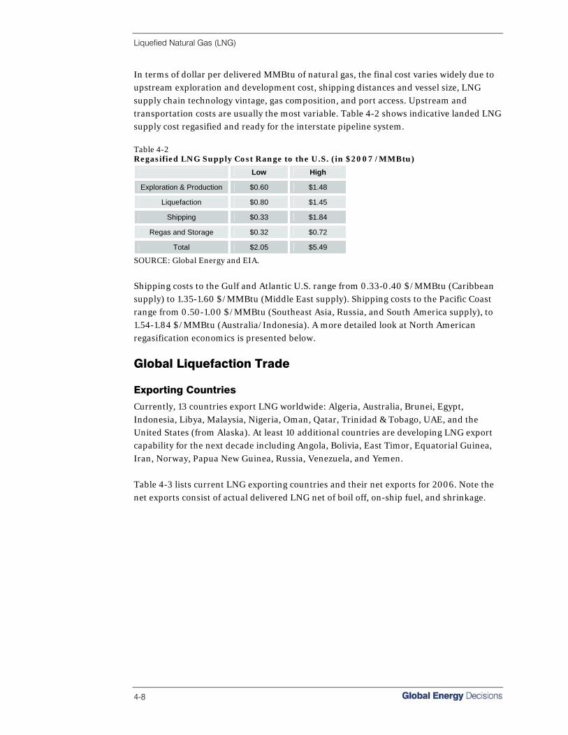
Liquefied Natural Gas (LNG)
4-8
In terms of dollar per delivered MMBtu of natural gas, the final cost varies widely due to upstream exploration and development cost, shipping distances and vessel size, LNG supply chain technology vintage, gas composition, and port access. Upstream and transportation costs are usually the most variable. Table 4-2 shows indicative landed LNG supply cost regasified and ready for the interstate pipeline system. Table 4-2 Regasified LNG Supply Cost Range to the U.S. (in $2007 /MMBtu)
Low High
Exploration & Production $0.60 $1.48
Liquefaction $0.80 $1.45
Shipping $0.33 $1.84
Regas and Storage $0.32 $0.72
Total $2.05 $5.49
SOURCE: Global Energy and EIA.
Shipping costs to the Gulf and Atlantic U.S. range from 0.33-0.40 $/MMBtu (Caribbean supply) to 1.35-1.60 $/MMBtu (Middle East supply). Shipping costs to the Pacific Coast range from 0.50-1.00 $/MMBtu (Southeast Asia, Russia, and South America supply), to 1.54-1.84 $/MMBtu (Australia/Indonesia). A more detailed look at North American regasification economics is presented below.
Global Liquefaction Trade Exporting Countries
Currently, 13 countries export LNG worldwide: Algeria, Australia, Brunei, Egypt, Indonesia, Libya, Malaysia, Nigeria, Oman, Qatar, Trinidad & Tobago, UAE, and the United States (from Alaska). At least 10 additional countries are developing LNG export capability for the next decade including Angola, Bolivia, East Timor, Equatorial Guinea, Iran, Norway, Papua New Guinea, Russia, Venezuela, and Yemen. Table 4-3 lists current LNG exporting countries and their net exports for 2006. Note the net exports consist of actual delivered LNG net of boil off, on-ship fuel, and shrinkage.
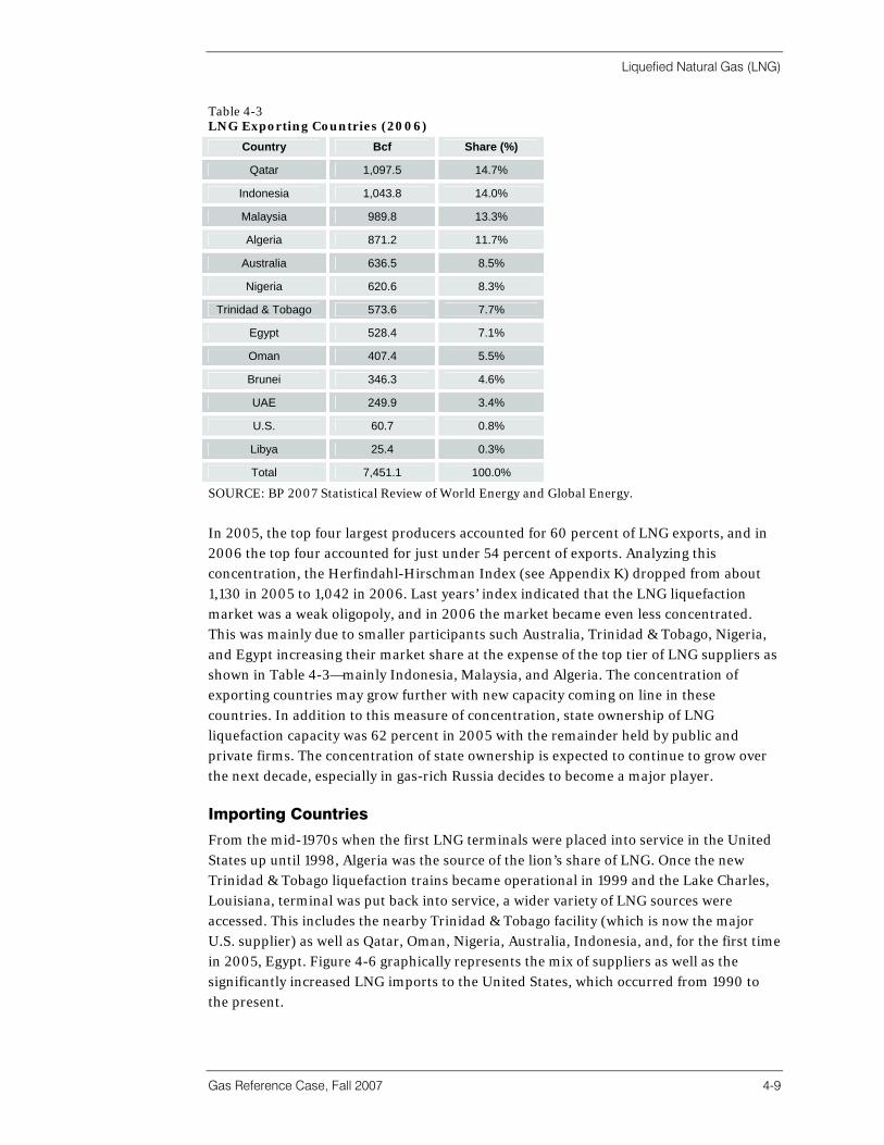
Liquefied Natural Gas (LNG)
Gas Reference Case, Fall 2007 4-9
Table 4-3 LNG Exporting Countries (2006)
Country Bcf Share (%)
Qatar 1,097.5 14.7%
Indonesia 1,043.8 14.0%
Malaysia 989.8 13.3%
Algeria 871.2 11.7%
Australia 636.5 8.5%
Nigeria 620.6 8.3%
Trinidad & Tobago 573.6 7.7%
Egypt 528.4 7.1%
Oman 407.4 5.5%
Brunei 346.3 4.6%
UAE 249.9 3.4%
U.S. 60.7 0.8%
Libya 25.4 0.3%
Total 7,451.1 100.0%
SOURCE: BP 2007 Statistical Review of World Energy and Global Energy.
In 2005, the top four largest producers accounted for 60 percent of LNG exports, and in 2006 the top four accounted for just under 54 percent of exports. Analyzing this concentration, the Herfindahl-Hirschman Index (see Appendix K) dropped from about 1,130 in 2005 to 1,042 in 2006. Last years’ index indicated that the LNG liquefaction market was a weak oligopoly, and in 2006 the market became even less concentrated. This was mainly due to smaller participants such Australia, Trinidad & Tobago, Nigeria, and Egypt increasing their market share at the expense of the top tier of LNG suppliers as shown in Table 4-3—mainly Indonesia, Malaysia, and Algeria. The concentration of exporting countries may grow further with new capacity coming on line in these countries. In addition to this measure of concentration, state ownership of LNG liquefaction capacity was 62 percent in 2005 with the remainder held by public and private firms. The concentration of state ownership is expected to continue to grow over the next decade, especially in gas-rich Russia decides to become a major player. Importing Countries
From the mid-1970s when the first LNG terminals were placed into service in the United States up until 1998, Algeria was the source of the lion’s share of LNG. Once the new Trinidad & Tobago liquefaction trains became operational in 1999 and the Lake Charles, Louisiana, terminal was put back into service, a wider variety of LNG sources were accessed. This includes the nearby Trinidad & Tobago facility (which is now the major U.S. supplier) as well as Qatar, Oman, Nigeria, Australia, Indonesia, and, for the first time in 2005, Egypt. Figure 4-6 graphically represents the mix of suppliers as well as the significantly increased LNG imports to the United States, which occurred from 1990 to the present.

Liquefied Natural Gas (LNG)
4-10
Figure 4-6 LNG Importing Countries; 1990-2006
0
100000
200000
300000
400000
500000
600000
700000
1990 1991 1992 1993 1994 1995 1996 1997 1998 1999 2000 2001 2002 2003 2004 2005 2006
MM
CF
Algeria
Trinidad & Tobago
Egypt
Australia
Qatar
Oman
Nigeria
Malaysia
Other (UAE, Brunei,Indonesia, etc.)
Average of 215 tanker deliveriesper year in the last 3 years.
SOURCE: Global Energy.
Global Liquefaction Projections Global LNG Supply
Figure 4-7 shows the current and proposed global liquefaction capacity in millions of tonnes per year. At the present time 76 million tons per year is under construction and projected to be on line by 2012. Another 57 million tons per year of incremental capacity is in the engineering stage with 36 million tons planned to be on line by 2012. Assuming these construction schedules can be met, worldwide liquefaction capacity could increase by 57 percent within five years. Note, converted into Bcf after shipping and other uses, one million tonnes is equivalent to about 45 Bcf available into the interstate pipeline grid after losses, boil-off, on ship use, and regasification plant usage. This amount varies due to a variety of factors such as plant technology employed, age of the facilities, season, and shipping distances. Using this conversion ratio means that globally, about 24.3 Bcf/d is available to end users currently, and over 41 Bcf/d is expected by 2012.

Liquefied Natural Gas (LNG)
Gas Reference Case, Fall 2007 4-11
Figure 4-7 Global Liquefaction Capacity (Million Tonnes/Year)
0
50
100
150
200
250
300
350
400
450
500
2007 2009 2011 2013 2015 2017 2019 2021
Mill
ion
Tonn
es p
er Y
ear
PlanningEngineeringConstructionExisting
SOURCE: Global Energy.
The current worldwide ratio of regasification capacity to liquefaction capacity is 2.1 to 1 indicating an LNG “sellers market.” Additionally, this ratio is forecasted to increase to over 3 to 1 by 2020 as regas terminals are put into service faster than the more expensive liquefaction terminals. In Global Energy’s opinion, the constraint on global liquefaction capacity and its growth are the most significant constraints facing North American (and other) markets—not NIMBY or other regasification siting and permitting issues.
Global LNG Demand In 2006, the world consumed about 101 Tcf of natural gas (up 2.5 percent from 2005) of which about 27 percent was consumed by the U.S., Canada, and Mexico. Overall, LNG supplied 7.5 Tcf of this global natural gas demand (up 13 percent), while Japan accounted for 39 percent of world LNG imports in 2006, down from over 45 percent in 2004. In 2006, the United States consumed just 8 percent of the world’s LNG supply at just over 523 Bcf, or approximately 2.4 percent, of its demand. Also in 2006, 17 countries imported LNG. Presently there are 52 plants operating worldwide with numerous projects under construction. The United Kingdom and Mexico are the latest countries to begin LNG imports. Over the next five years at least seven additional countries are looking towards LNG to meet incremental demand. These include Brazil, Canada, China, Jamaica, New Zealand, Singapore, and Thailand. Japan and South Korea are the largest importers of LNG and have had the longest history of importing significant quantities. Overall they accounted for nearly 55 percent of the total demand (down 2 percent from 2005). Table 4-4 ranks LNG importing countries by their size and share of the world total.
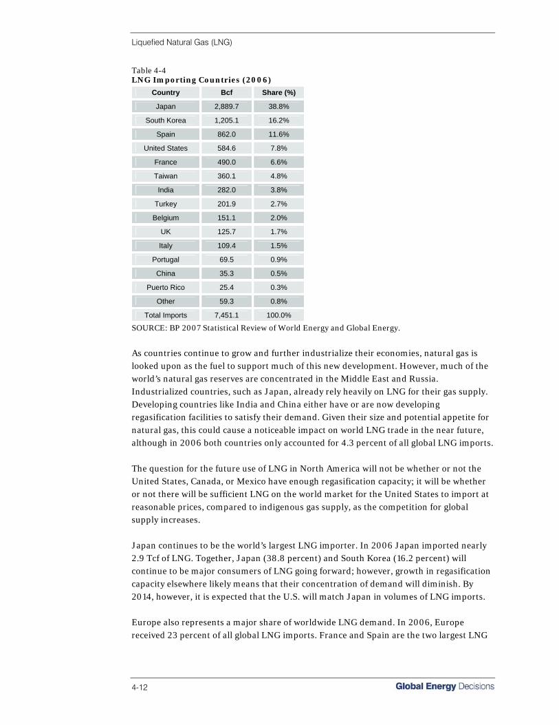
Liquefied Natural Gas (LNG)
4-12
Table 4-4 LNG Importing Countries (2006)
Country Bcf Share (%)
Japan 2,889.7 38.8%
South Korea 1,205.1 16.2%
Spain 862.0 11.6%
United States 584.6 7.8%
France 490.0 6.6%
Taiwan 360.1 4.8%
India 282.0 3.8%
Turkey 201.9 2.7%
Belgium 151.1 2.0%
UK 125.7 1.7%
Italy 109.4 1.5%
Portugal 69.5 0.9%
China 35.3 0.5%
Puerto Rico 25.4 0.3%
Other 59.3 0.8%
Total Imports 7,451.1 100.0%
SOURCE: BP 2007 Statistical Review of World Energy and Global Energy.
As countries continue to grow and further industrialize their economies, natural gas is looked upon as the fuel to support much of this new development. However, much of the world’s natural gas reserves are concentrated in the Middle East and Russia. Industrialized countries, such as Japan, already rely heavily on LNG for their gas supply. Developing countries like India and China either have or are now developing regasification facilities to satisfy their demand. Given their size and potential appetite for natural gas, this could cause a noticeable impact on world LNG trade in the near future, although in 2006 both countries only accounted for 4.3 percent of all global LNG imports. The question for the future use of LNG in North America will not be whether or not the United States, Canada, or Mexico have enough regasification capacity; it will be whether or not there will be sufficient LNG on the world market for the United States to import at reasonable prices, compared to indigenous gas supply, as the competition for global supply increases. Japan continues to be the world’s largest LNG importer. In 2006 Japan imported nearly 2.9 Tcf of LNG. Together, Japan (38.8 percent) and South Korea (16.2 percent) will continue to be major consumers of LNG going forward; however, growth in regasification capacity elsewhere likely means that their concentration of demand will diminish. By 2014, however, it is expected that the U.S. will match Japan in volumes of LNG imports. Europe also represents a major share of worldwide LNG demand. In 2006, Europe received 23 percent of all global LNG imports. France and Spain are the two largest LNG
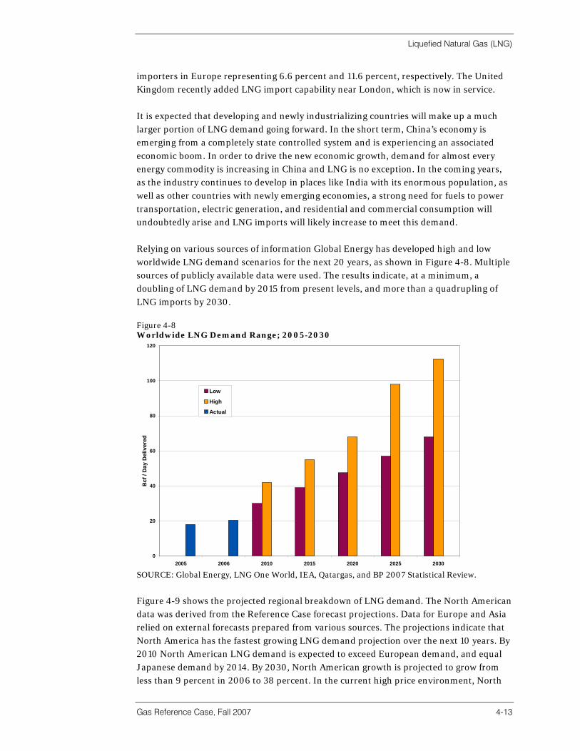
Liquefied Natural Gas (LNG)
Gas Reference Case, Fall 2007 4-13
importers in Europe representing 6.6 percent and 11.6 percent, respectively. The United Kingdom recently added LNG import capability near London, which is now in service. It is expected that developing and newly industrializing countries will make up a much larger portion of LNG demand going forward. In the short term, China’s economy is emerging from a completely state controlled system and is experiencing an associated economic boom. In order to drive the new economic growth, demand for almost every energy commodity is increasing in China and LNG is no exception. In the coming years, as the industry continues to develop in places like India with its enormous population, as well as other countries with newly emerging economies, a strong need for fuels to power transportation, electric generation, and residential and commercial consumption will undoubtedly arise and LNG imports will likely increase to meet this demand. Relying on various sources of information Global Energy has developed high and low worldwide LNG demand scenarios for the next 20 years, as shown in Figure 4-8. Multiple sources of publicly available data were used. The results indicate, at a minimum, a doubling of LNG demand by 2015 from present levels, and more than a quadrupling of LNG imports by 2030. Figure 4-8 Worldwide LNG Demand Range; 2005-2030
0
20
40
60
80
100
120
2005 2006 2010 2015 2020 2025 2030
Bcf
/ D
ay D
eliv
ered
Low
High
Actual
SOURCE: Global Energy, LNG One World, IEA, Qatargas, and BP 2007 Statistical Review.
Figure 4-9 shows the projected regional breakdown of LNG demand. The North American data was derived from the Reference Case forecast projections. Data for Europe and Asia relied on external forecasts prepared from various sources. The projections indicate that North America has the fastest growing LNG demand projection over the next 10 years. By 2010 North American LNG demand is expected to exceed European demand, and equal Japanese demand by 2014. By 2030, North American growth is projected to grow from less than 9 percent in 2006 to 38 percent. In the current high price environment, North
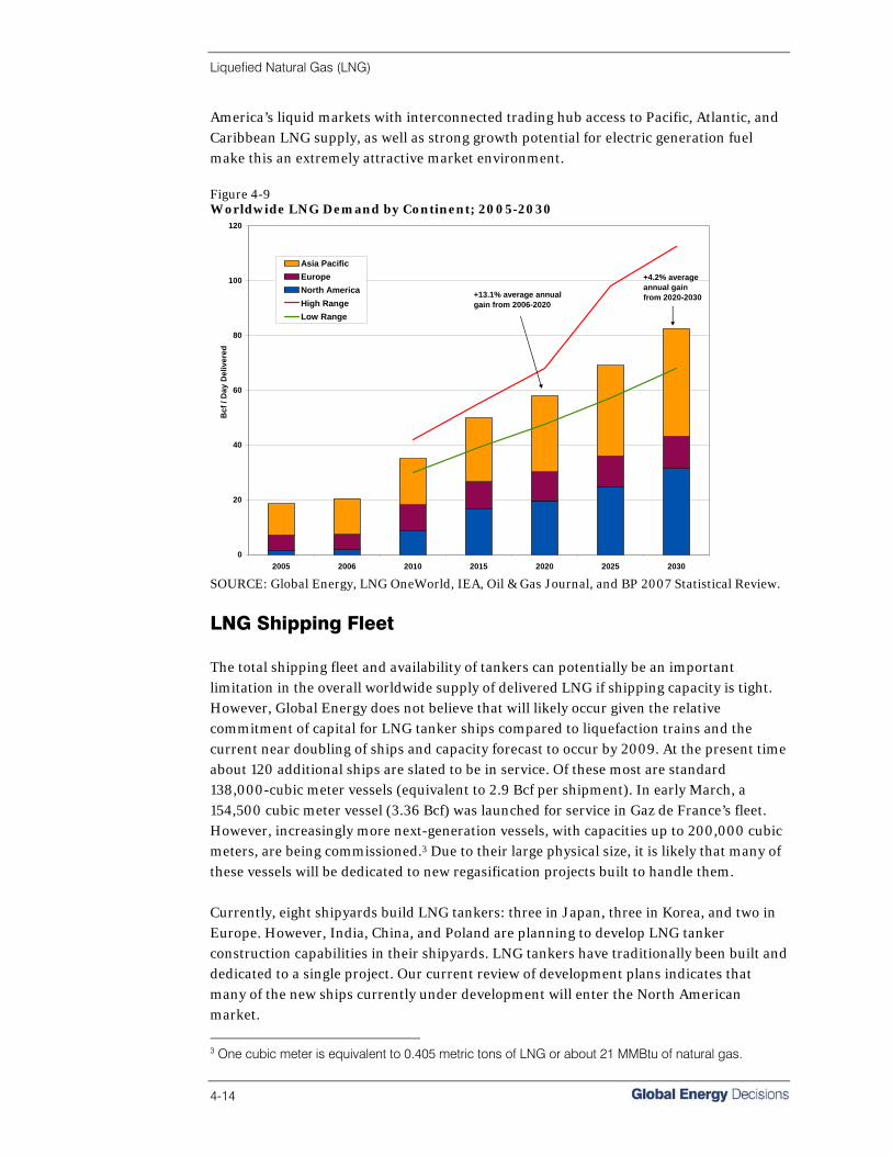
Liquefied Natural Gas (LNG)
4-14
America’s liquid markets with interconnected trading hub access to Pacific, Atlantic, and Caribbean LNG supply, as well as strong growth potential for electric generation fuel make this an extremely attractive market environment. Figure 4-9 Worldwide LNG Demand by Continent; 2005-2030
0
20
40
60
80
100
120
2005 2006 2010 2015 2020 2025 2030
Bcf
/ D
ay D
eliv
ered
Asia PacificEuropeNorth AmericaHigh RangeLow Range
+13.1% average annual gain from 2006-2020
+4.2% average annual gainfrom 2020-2030
SOURCE: Global Energy, LNG OneWorld, IEA, Oil & Gas Journal, and BP 2007 Statistical Review.
LNG Shipping Fleet The total shipping fleet and availability of tankers can potentially be an important limitation in the overall worldwide supply of delivered LNG if shipping capacity is tight. However, Global Energy does not believe that will likely occur given the relative commitment of capital for LNG tanker ships compared to liquefaction trains and the current near doubling of ships and capacity forecast to occur by 2009. At the present time about 120 additional ships are slated to be in service. Of these most are standard 138,000-cubic meter vessels (equivalent to 2.9 Bcf per shipment). In early March, a 154,500 cubic meter vessel (3.36 Bcf) was launched for service in Gaz de France’s fleet. However, increasingly more next-generation vessels, with capacities up to 200,000 cubic meters, are being commissioned.3 Due to their large physical size, it is likely that many of these vessels will be dedicated to new regasification projects built to handle them. Currently, eight shipyards build LNG tankers: three in Japan, three in Korea, and two in Europe. However, India, China, and Poland are planning to develop LNG tanker construction capabilities in their shipyards. LNG tankers have traditionally been built and dedicated to a single project. Our current review of development plans indicates that many of the new ships currently under development will enter the North American market.
3 One cubic meter is equivalent to 0.405 metric tons of LNG or about 21 MMBtu of natural gas.
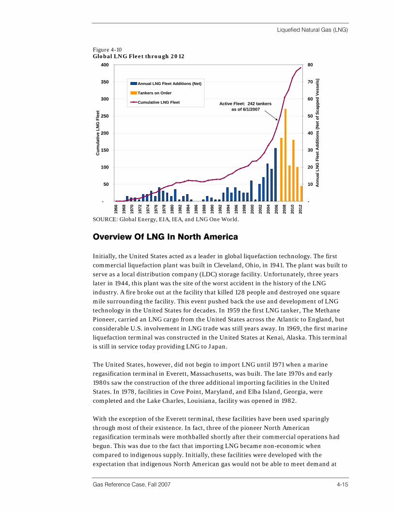
Liquefied Natural Gas (LNG)
Gas Reference Case, Fall 2007 4-15
Figure 4-10 Global LNG Fleet through 2012
-
50
100
150
200
250
300
350
400
1966
1968
1970
1972
1974
1976
1978
1980
1982
1984
1986
1988
1990
1992
1994
1996
1998
2000
2002
2004
2006
2008
2010
2012
Cum
ulat
ive
LNG
Fle
et
-
10
20
30
40
50
60
70
80
Ann
ual L
NG
Fle
et A
dditi
ons
(Net
of S
capp
ed V
esse
ls)
Annual LNG Fleet Additions (Net)
Tankers on Order
Cumulative LNG Fleet Active Fleet: 242 tankers as of 6/1/2007
SOURCE: Global Energy, EIA, IEA, and LNG One World.
Overview Of LNG In North America Initially, the United States acted as a leader in global liquefaction technology. The first commercial liquefaction plant was built in Cleveland, Ohio, in 1941. The plant was built to serve as a local distribution company (LDC) storage facility. Unfortunately, three years later in 1944, this plant was the site of the worst accident in the history of the LNG industry. A fire broke out at the facility that killed 128 people and destroyed one square mile surrounding the facility. This event pushed back the use and development of LNG technology in the United States for decades. In 1959 the first LNG tanker, The Methane Pioneer, carried an LNG cargo from the United States across the Atlantic to England, but considerable U.S. involvement in LNG trade was still years away. In 1969, the first marine liquefaction terminal was constructed in the United States at Kenai, Alaska. This terminal is still in service today providing LNG to Japan. The United States, however, did not begin to import LNG until 1971 when a marine regasification terminal in Everett, Massachusetts, was built. The late 1970s and early 1980s saw the construction of the three additional importing facilities in the United States. In 1978, facilities in Cove Point, Maryland, and Elba Island, Georgia, were completed and the Lake Charles, Louisiana, facility was opened in 1982. With the exception of the Everett terminal, these facilities have been used sparingly through most of their existence. In fact, three of the pioneer North American regasification terminals were mothballed shortly after their commercial operations had begun. This was due to the fact that importing LNG became non-economic when compared to indigenous supply. Initially, these facilities were developed with the expectation that indigenous North American gas would not be able to meet demand at
Liquefied Natural Gas (LNG)
4-16
acceptable prices. Many technical and market factors proved this premise to be wrong. A major driver of the demise of the early North American LNG market was the development of two rather untapped North American supply regions—the Western Canadian Sedimentary Basin and the San Juan Basin. However, with the decrease in production of gas from conventional fields over the decades, increasing demand and the resultant increase in natural gas prices since the beginning of 2000, interest in LNG imports has been rekindled. This first resulted in reopening several mothballed U.S. LNG terminals. The Lake Charles facility commenced operation in 1999 and the Elba Island and Cove Point facilities reopened in 2001 and 2003, respectively. Although greater volumes of LNG have been delivered in the past several years, the existing U.S. terminals are still not being used anywhere near full capacity. Looking at monthly data for 2006, cryogenic tanker deliveries have averaged 31 percent of maximum regasification capacity, varying from a high of 46 percent in May 2006 to a low of 25 percent in October 2006. Utilization should be at least twice this average number in order to achieve reasonable “per unit” economies by spreading fixed costs over higher volumes, and it remains to be seen if the parties can handle the tanker logistics of docking in various weather conditions, unloading their cargo quickly, roundtrip voyage, loading, and demurrage, etcetera, in order to fully utilize the terminals’ potential.4 Given current LNG price competitiveness, the expectation for demand growth and the outlook for stagnant North American natural gas production have caused a boom in new construction and expansion proposals on each U.S. coast as well as in Canada and Mexico. As we address below, many of these facilities have received regulatory approval and expect to be operational over the next few years. The future of LNG in North America rests on the industry’s ability to align the interests of market players and allow for the timely development of adequate infrastructure across the entire LNG value chain.
Outlook For Regasification In North America As of this writing, six regasification terminals were operating in the United States with a combined peak send out capacity of 6.5 Bcf/d. An additional seven Greenfield LNG and two expansion regasification projects are currently under way in North America.5 Of the seven Greenfield units, five are located in the U.S. with one in Mexico and another in Canada, each designed to serve U.S. markets, at least in part. Figure 4-11 shows total capacity in Bcf/d (max send out rate) by status through 2014 for LNG plants by coastline. The figure excludes facilities designed exclusively for the domestic Mexican market but includes under development and announced facilities along with operation, permitted, and under construction facilities.
4 Detention in port of a vessel, as in loading or unloading, beyond the time allowed or agreed upon usually resulting in monetary penalties for the disruption. 5 Our analysis considers facilities in the U.S., Canada, Mexico, and the Bahamas given the close proximity to the U.S. coastline. We have excluded the existing Puerto Rico regasification facility as it is designed to serve that island’s load only.

Liquefied Natural Gas (LNG)
Gas Reference Case, Fall 2007 4-17
According to the sponsors of projects currently under construction, as much as 11 Bcf/d (about 18 percent of total U.S. gas demand) will be on line by 2008 in the Gulf of Mexico alone. Another 1 Bcf/d each on the Atlantic Coast and another 2.5 Bcf/d on the Pacific Coast is under construction. The Atlantic facility is Irving Oil’s Canaport facility located in New Brunswick and the Pacific facility is Sempra’s Costa Azul. Figure 4-11 Existing, Under Construction and Proposed Regasification Capacity
-
1,000
2,000
3,000
4,000
5,000
6,000
7,000
8,000
2009 2010 2011 2008 2009 2010 2012 2010 2011 2012 2013 2014
Approved Construction Proposed
mm
cf/d
AtlanticGulfPacific
SOURCE: Global Energy.
Figure 4-12 Cumulative Existing, Under Construction and Proposed Regasification Capacity
-
10,000
20,000
30,000
40,000
50,000
60,000
70,000
2007 2008 2009 2010 2011 2012 2013 2014
mm
cf/d
PacificGulfAtlantic
SOURCE: Global Energy.
Figure 4-13 eliminates the equivalent of 33 Bcf/d of announced capacity that has not yet been approved by regulators shown in Figure 4-12. The figure shows that significant
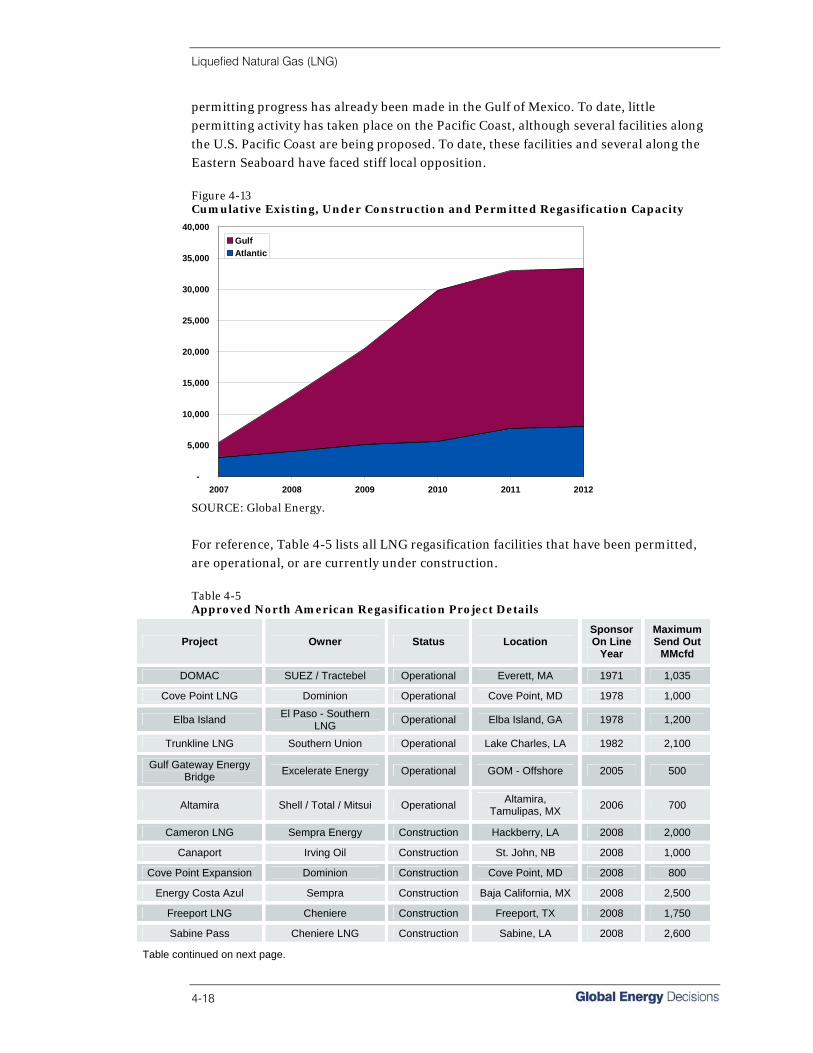
Liquefied Natural Gas (LNG)
4-18
permitting progress has already been made in the Gulf of Mexico. To date, little permitting activity has taken place on the Pacific Coast, although several facilities along the U.S. Pacific Coast are being proposed. To date, these facilities and several along the Eastern Seaboard have faced stiff local opposition. Figure 4-13 Cumulative Existing, Under Construction and Permitted Regasification Capacity
-
5,000
10,000
15,000
20,000
25,000
30,000
35,000
40,000
2007 2008 2009 2010 2011 2012
GulfAtlantic
SOURCE: Global Energy.
For reference, Table 4-5 lists all LNG regasification facilities that have been permitted, are operational, or are currently under construction. Table 4-5 Approved North American Regasification Project Details
Project Owner Status Location Sponsor On Line
Year
Maximum Send Out
MMcfd
DOMAC SUEZ / Tractebel Operational Everett, MA 1971 1,035
Cove Point LNG Dominion Operational Cove Point, MD 1978 1,000
Elba Island El Paso - Southern LNG Operational Elba Island, GA 1978 1,200
Trunkline LNG Southern Union Operational Lake Charles, LA 1982 2,100
Gulf Gateway Energy Bridge Excelerate Energy Operational GOM - Offshore 2005 500
Altamira Shell / Total / Mitsui Operational Altamira, Tamulipas, MX 2006 700
Cameron LNG Sempra Energy Construction Hackberry, LA 2008 2,000
Canaport Irving Oil Construction St. John, NB 2008 1,000
Cove Point Expansion Dominion Construction Cove Point, MD 2008 800
Energy Costa Azul Sempra Construction Baja California, MX 2008 2,500
Freeport LNG Cheniere Construction Freeport, TX 2008 1,750
Sabine Pass Cheniere LNG Construction Sabine, LA 2008 2,600
Table continued on next page.
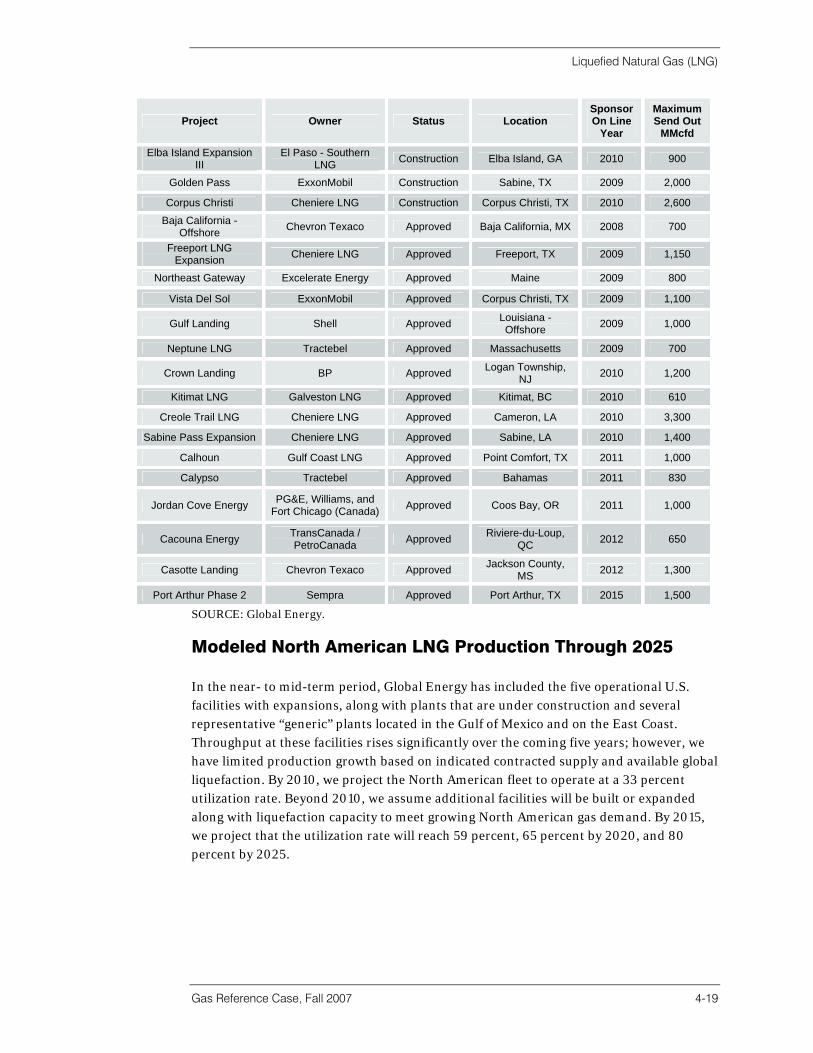
Liquefied Natural Gas (LNG)
Gas Reference Case, Fall 2007 4-19
Project Owner Status Location Sponsor On Line
Year
Maximum Send Out
MMcfd
Elba Island Expansion III
El Paso - Southern LNG Construction Elba Island, GA 2010 900
Golden Pass ExxonMobil Construction Sabine, TX 2009 2,000
Corpus Christi Cheniere LNG Construction Corpus Christi, TX 2010 2,600
Baja California - Offshore Chevron Texaco Approved Baja California, MX 2008 700
Freeport LNG Expansion Cheniere LNG Approved Freeport, TX 2009 1,150
Northeast Gateway Excelerate Energy Approved Maine 2009 800
Vista Del Sol ExxonMobil Approved Corpus Christi, TX 2009 1,100
Gulf Landing Shell Approved Louisiana - Offshore 2009 1,000
Neptune LNG Tractebel Approved Massachusetts 2009 700
Crown Landing BP Approved Logan Township, NJ 2010 1,200
Kitimat LNG Galveston LNG Approved Kitimat, BC 2010 610
Creole Trail LNG Cheniere LNG Approved Cameron, LA 2010 3,300
Sabine Pass Expansion Cheniere LNG Approved Sabine, LA 2010 1,400
Calhoun Gulf Coast LNG Approved Point Comfort, TX 2011 1,000
Calypso Tractebel Approved Bahamas 2011 830
Jordan Cove Energy PG&E, Williams, and Fort Chicago (Canada) Approved Coos Bay, OR 2011 1,000
Cacouna Energy TransCanada / PetroCanada Approved Riviere-du-Loup,
QC 2012 650
Casotte Landing Chevron Texaco Approved Jackson County, MS 2012 1,300
Port Arthur Phase 2 Sempra Approved Port Arthur, TX 2015 1,500
SOURCE: Global Energy.
Modeled North American LNG Production Through 2025 In the near- to mid-term period, Global Energy has included the five operational U.S. facilities with expansions, along with plants that are under construction and several representative “generic” plants located in the Gulf of Mexico and on the East Coast. Throughput at these facilities rises significantly over the coming five years; however, we have limited production growth based on indicated contracted supply and available global liquefaction. By 2010, we project the North American fleet to operate at a 33 percent utilization rate. Beyond 2010, we assume additional facilities will be built or expanded along with liquefaction capacity to meet growing North American gas demand. By 2015, we project that the utilization rate will reach 59 percent, 65 percent by 2020, and 80 percent by 2025.

Liquefied Natural Gas (LNG)
4-20
Table 4-6 Modeled Regasification Terminal Delivery through 2025 (Annual Average MMcf/d and Utilization Rate)
LNG Facilities, Imports & Utilization Rate 2010 2015 2020 2025
Altamira 239 356 391 527
% 34% 50% 55% 74%
British Columbia 33 273 269 391
% 5% 44% 43% 63%
Cameron 227 809 895 1,157
% 15% 53% 59% 76%
Canaport 167 565 588 737
% 16% 56% 58% 73%
Cove Point 1,101 1,223 1,250 1,493
% 60% 67% 69% 82%
Distrigas 665 725 696 763
% 63% 69% 66% 72%
Elba Island 807 1,404 1,442 1,717
% 46% 66% 68% 81%
Freeport 1,595 1,756 1,679 1,988
% 54% 60% 57% 68%
GED Costa Azul 826 1,125 1,182 1,243
% 38% 44% 47% 49%
GED Generic Bahamas 525 528 610
% 62% 63% 72%
GED Generic Baja 454 479 504
% 45% 47% 50%
GED Generic Gulf 1,374
% 68%
GED Generic Mid Atlantic 575 578
% 28% 28%
GED Generic Northeast 1,170 1,330
% 58% 66%
GED Generic Pacific 1,160 1,442
% 57% 71%
99GED Generic Québec 643 582 663
% 63% 57% 65%
GED Generic Texas 1,202 1,154 1,399
% 59% 57% 69%
Golden Pass 366 1,490 1,473 1,618
% 18% 74% 73% 80%
Gulf Gateway 127 140 140 140
% 23% 25% 25% 25%
Lake Charles 1,044 1,100 1,126 1,383
% 57% 60% 62% 76%
Neptune 29 248 244 294
% 7% 62% 61% 73%
Table continued on next page.

Liquefied Natural Gas (LNG)
Gas Reference Case, Fall 2007 4-21
LNG Facilities, Imports & Utilization Rate 2010 2015 2020 2025
Sabine Pass 1,430 2,569 2,821 3,453
% 33% 59% 65% 80%
SOURCE: Global Energy.
Figure 4-14 shows a graphic representation of the increasing North American LNG vaporization capacity, production and percentage of utilization, which, prior to 2007, is essentially all U.S. data. North America has turned a corner in 2007 where LNG is more than just a small “side show” of supply, but an integral part of its infrastructure. There will be an exponential growth in number of regas facilities and usage. Additionally, within five years it will be obvious that a transition has occurred where natural gas supply for the U.S. is not only dependent on countries outside the U.S. and outside North American, but possibly dependent on Middle East countries, just like for crude oil. Figure 4-14 North American Regasification Capacity, Production and Utilization Percentage
0
5
10
15
20
25
30
35
40
2001 2002 2003 2004 2005 2006 2007 2008 2009 2010 2015 2020 2025
Bcf
/d
0%
10%
20%
30%
40%
50%
60%
70%
80%LNG ProductionLNG Max CapacityUtilization Percentage
Actual
SOURCE: Global Energy.
LNG Concerns
Despite the need to find new gas sources to supply the United States market, not everyone is enamored with LNG. LNG has various opponents who discourage its use for a multitude of reasons. Major concerns exist over siting and perceived safety. The opposition to LNG has played out on the local level, with communities attempting to ban LNG facilities and also on the national level as states battle FERC for jurisdiction over the right to site facilities in certain locations. Be it local or national issues, the resistance to LNG usually comes down to concerns and fears revolving around environmental impact, terrorism, or accidents. Further, others cite the growing effect of NIMBY (Not in My Back Yard)—stopping industrialization for its own sake, which can also play an important part

Liquefied Natural Gas (LNG)
4-22
in shaping development. In addition to these political concerns is the major commercial issue of gas quality interchangeability and its resultant costs. LNG facilities are sometimes proposed in areas that cause concerns about local fish and wildlife. ExxonMobil’s proposed Golden Pass LNG terminal, if approved, would be built near Sabine Pass, Texas. This is an ideal location for an LNG terminal due to its close proximity to existing natural gas infrastructure and because it is located along a deep water port where large LNG tankers can travel and unload cargo. However, siting an LNG terminal in this spot has the potential to adversely affect wetlands, fish, wildlife, and endangered species. A variety of migrating birds use the area’s forests as nesting grounds and their habitat may be threatened by the proposed terminal and associated pipelines. These issues concerning local wildlife are being evaluated by the U.S. Fish and Wildlife Service and will need to be addressed before the project can go ahead. In addition, offshore LNG regasification facilities also face strong opposition, even though they are further from human habitation and do not constrain marine life near coastal and inland waterways used by onshore LNG facilities. This type of situation is not uncommon. LNG facilities have the potential to alter the landscape where they are built, and when new terminals are proposed in areas with an abundance of wildlife or natural beauty, local concerns about the potential environmental impact generally follow. Another reason proposed LNG facilities struggle to win approval are the fears of terrorism in America ever since 9/11. Opponents to LNG development argue that LNG tankers and terminals present a potential terrorist target, especially when a facility is located near a large population center. However, LNG is only flammable as methane vapor and within narrow concentrations ranging from 5 to 15 percent in the atmosphere. LNG is also not explosive in an unconfined environment. Despite these facts, it would still be possible for a terrorist attack involving LNG infrastructure to be extremely destructive. Much of the local opposition to KeySpan’s proposed LNG facility in Providence, Rhode Island, revolves around fears of terrorism. At a recent meeting held by Rhode Island Attorney General Patrick Lynch, Lynch showed a slide of an LNG tanker about to be struck by a superimposed airplane, “this is possible, and the federal government is not equipped [to handle it].”6 Richard A. Clarke, the security expert and former counterterrorism chief for many U.S. administrations, stated in his book, Against All Enemies, that the FBI learned in December 1999 that Al Qaeda suspects had entered the United States on LNG tankers that dock at the DistriGas port in Everett, Massachusetts. It has also been reported that “more than a dozen” stowaways with Al Qaeda ties had entered the United States in the late 1990s on tankers making deliveries to the LNG terminal near Boston. According to Roger Cressey, Clarke’s second-in-command, “The LNG tanker was an underground railroad for these guys to come into the country illegally.” The FBI has publicly conceded that one of the men later convicted in the so called Millennium plot to bomb Los Angeles International Airport, Abdelghani Meskini, arrived in Boston as a stowaway on an Algerian tanker in January 1995.
6 The Herald News, March 25, 2005.
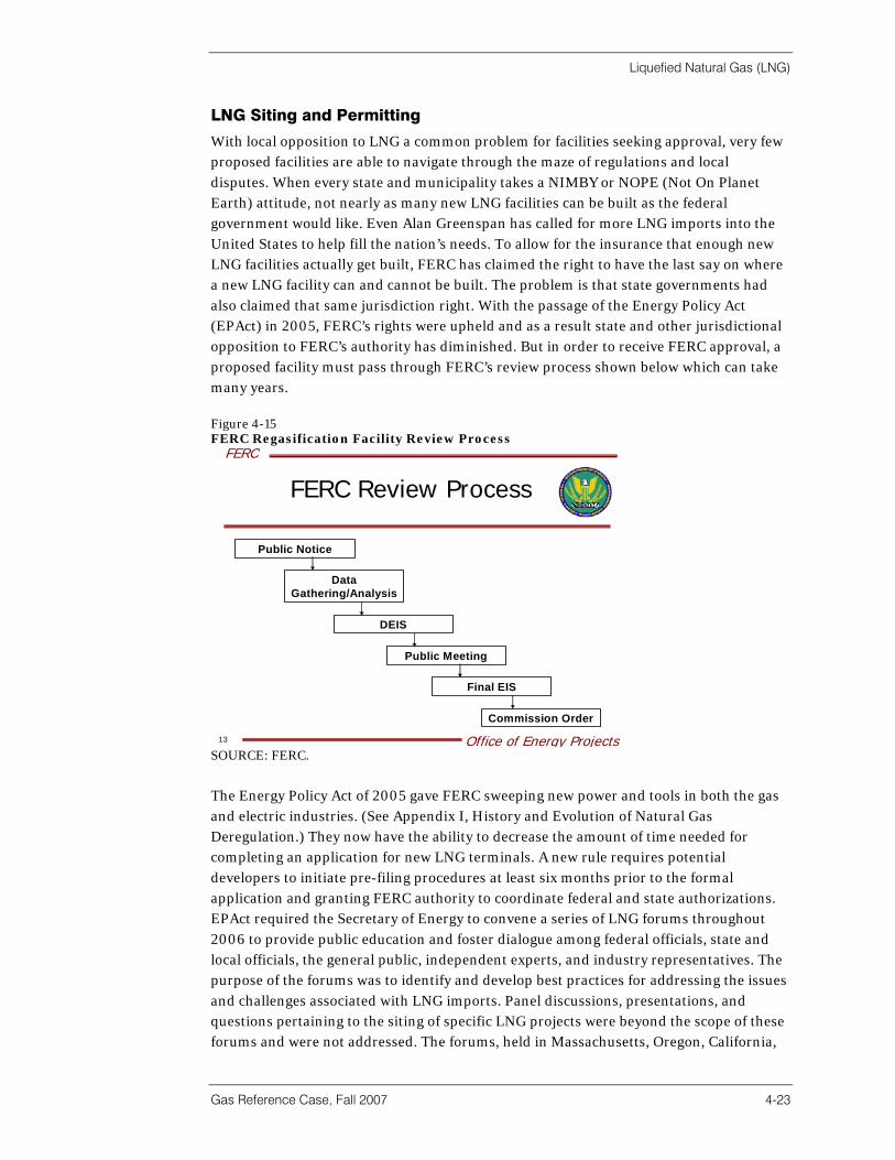
Liquefied Natural Gas (LNG)
Gas Reference Case, Fall 2007 4-23
LNG Siting and Permitting
With local opposition to LNG a common problem for facilities seeking approval, very few proposed facilities are able to navigate through the maze of regulations and local disputes. When every state and municipality takes a NIMBY or NOPE (Not On Planet Earth) attitude, not nearly as many new LNG facilities can be built as the federal government would like. Even Alan Greenspan has called for more LNG imports into the United States to help fill the nation’s needs. To allow for the insurance that enough new LNG facilities actually get built, FERC has claimed the right to have the last say on where a new LNG facility can and cannot be built. The problem is that state governments had also claimed that same jurisdiction right. With the passage of the Energy Policy Act (EPAct) in 2005, FERC’s rights were upheld and as a result state and other jurisdictional opposition to FERC’s authority has diminished. But in order to receive FERC approval, a proposed facility must pass through FERC’s review process shown below which can take many years. Figure 4-15 FERC Regasification Facility Review Process
FERC
Office of Energy Projects13
FERC Review Process
Public Notice
Data Gathering/Analysis
DEIS
Public Meeting
Final EIS
Commission Order
SOURCE: FERC.
The Energy Policy Act of 2005 gave FERC sweeping new power and tools in both the gas and electric industries. (See Appendix I, History and Evolution of Natural Gas Deregulation.) They now have the ability to decrease the amount of time needed for completing an application for new LNG terminals. A new rule requires potential developers to initiate pre-filing procedures at least six months prior to the formal application and granting FERC authority to coordinate federal and state authorizations. EPAct required the Secretary of Energy to convene a series of LNG forums throughout 2006 to provide public education and foster dialogue among federal officials, state and local officials, the general public, independent experts, and industry representatives. The purpose of the forums was to identify and develop best practices for addressing the issues and challenges associated with LNG imports. Panel discussions, presentations, and questions pertaining to the siting of specific LNG projects were beyond the scope of these forums and were not addressed. The forums, held in Massachusetts, Oregon, California,
Liquefied Natural Gas (LNG)
4-24
and Texas were intended to be educational events and not intended to be public hearings related to any siting or licensing proceeding. However, states and others can and do succeed at stopping LNG development, notwithstanding the EPAct. The Weavers Cove, Massachusetts, LNG development is a prime example. The facility was approved by FERC, but has faced strong opposition by others. Recently the legislation to restrict LNG tankers in Massachusetts waters was enacted after being passed in both the House and Senate. The legislation states:
“…no company can operate an LNG vessel under a bridge if the vessel has a horizontal clearance of 250 feet or less unless the beam of the vessel is equal to or less than two-thirds of the horizontal clearance of the bridge. Any violation of the safe clearance requirements established in the bill would subject the operator to civil penalty not to exceed $1 million. The bill includes a caveat to affect only transportation of LNG to facilities that were built or expanded after July 1, 2006.”7
Regasification Economics In North America On a full cycle basis (accounting for exploration, development, and production costs), landed LNG costs from many supply regions are presently competitive with production out of many traditional North American supply basins. At the time of writing with Henry Hub gas prices above $6.75/MMBtu, the potential economic returns for LNG projects are fairly attractive. Our research indicates that LNG, even from the most expensive supply regions, has the potential to displace GOM onshore and offshore production on both a full-cycle replacement cost and marginal cost basis. Marginal cost is defined as the full-cycle recovery cost (export wellhead to long-haul import pipeline) minus fixed capital cost (return on equity and of debt). Global Energy research indicates that when the Henry Hub gas price is $6/MMBtu (for royalty and tax burden reductions), incremental indigenous Gulf of Mexico non-associated gas has a full-cycle replacement cost of $ 2.75 to 3.75 /MMBtu. In comparison regasified LNG has a full-cycle replacement cost ranging from $ 2.25 to 2.75 /MMBtu from the Caribbean to GOM to $ 3.35-4.15 /MMBtu from Africa or Norway to GOM, based on wellhead net-back price of $ 0.30 to just over 1.00 /MMBtu. In addition, the marginal cost of gas from the Gulf of Mexico is generally 65 percent of the total cost into the interstate pipeline, compared with regasified LNG supplies at 50 percent. Marginal costs for the Gulf of Mexico are $ 1.80 to $2.75 /MMBtu, compared to regasified LNG at approximately $ 0.90 from the Caribbean to $ 1.75 /MMBtu from Australia. In conclusion, the marginal cost for regasified LNG is approximately $ 0.05 to $1.60/MMBtu less than that of Gulf of Mexico gas, while the full cycle replacement cost of regasified LNG is approximately $ 0.25 to $1.50/MMBtu less than for Gulf gas, depending largely on shipping distance. LNG should therefore provide a floor price for U.S. indigenous gas based on a very competitive cost-of-service structure.
7 Natural Gas Intelligence, July 31, 2006.
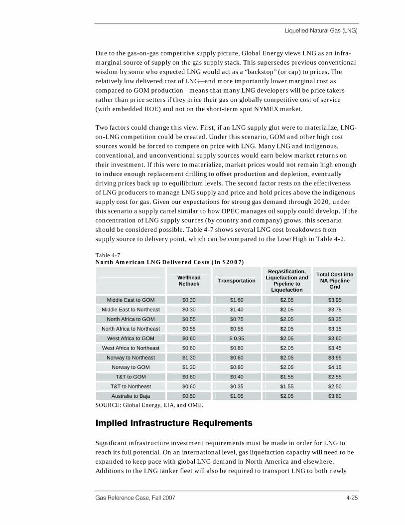
Liquefied Natural Gas (LNG)
Gas Reference Case, Fall 2007 4-25
Due to the gas-on-gas competitive supply picture, Global Energy views LNG as an infra-marginal source of supply on the gas supply stack. This supersedes previous conventional wisdom by some who expected LNG would act as a “backstop” (or cap) to prices. The relatively low delivered cost of LNG—and more importantly lower marginal cost as compared to GOM production—means that many LNG developers will be price takers rather than price setters if they price their gas on globally competitive cost of service (with embedded ROE) and not on the short-term spot NYMEX market. Two factors could change this view. First, if an LNG supply glut were to materialize, LNG-on-LNG competition could be created. Under this scenario, GOM and other high cost sources would be forced to compete on price with LNG. Many LNG and indigenous, conventional, and unconventional supply sources would earn below market returns on their investment. If this were to materialize, market prices would not remain high enough to induce enough replacement drilling to offset production and depletion, eventually driving prices back up to equilibrium levels. The second factor rests on the effectiveness of LNG producers to manage LNG supply and price and hold prices above the indigenous supply cost for gas. Given our expectations for strong gas demand through 2020, under this scenario a supply cartel similar to how OPEC manages oil supply could develop. If the concentration of LNG supply sources (by country and company) grows, this scenario should be considered possible. Table 4-7 shows several LNG cost breakdowns from supply source to delivery point, which can be compared to the Low/High in Table 4-2. Table 4-7 North American LNG Delivered Costs (In $2007)
Wellhead Netback Transportation
Regasification, Liquefaction and
Pipeline to Liquefaction
Total Cost into NA Pipeline
Grid
Middle East to GOM $0.30 $1.60 $2.05 $3.95
Middle East to Northeast $0.30 $1.40 $2.05 $3.75
North Africa to GOM $0.55 $0.75 $2.05 $3.35
North Africa to Northeast $0.55 $0.55 $2.05 $3.15
West Africa to GOM $0.60 $ 0.95 $2.05 $3.60
West Africa to Northeast $0.60 $0.80 $2.05 $3.45
Norway to Northeast $1.30 $0.60 $2.05 $3.95
Norway to GOM $1.30 $0.80 $2.05 $4.15
T&T to GOM $0.60 $0.40 $1.55 $2.55
T&T to Northeast $0.60 $0.35 $1.55 $2.50
Australia to Baja $0.50 $1.05 $2.05 $3.60
SOURCE: Global Energy, EIA, and OME.
Implied Infrastructure Requirements Significant infrastructure investment requirements must be made in order for LNG to reach its full potential. On an international level, gas liquefaction capacity will need to be expanded to keep pace with global LNG demand in North America and elsewhere. Additions to the LNG tanker fleet will also be required to transport LNG to both newly
Liquefied Natural Gas (LNG)
4-26
developing markets and expanding established markets. On a national level, the United States will need to increase regasification capacity and build the necessary storage facilities and transportation pipelines to accommodate the new influx of LNG. By 2015, our modeling suggests that North America may be importing about 13.6 Bcf/d equivalent of LNG. This represents a more than a 9-fold increase from the 1.45 Bcf/d imported on average from 2003 through 2006. By 2020, the forecast is for LNG to increase to 16.8 Bcf/d, a 11.5-fold increase, and by 2030 an increase to 23 Bcf/d, a 16-fold increase. This rise in U.S. demand for LNG will have to be accommodated by a corresponding increase in global liquefaction capacity. This capacity expansion will be spread out across various countries, including some that are already players in LNG exporting like Trinidad & Tobago, and others that will be new to the game, such as Iran and Russia.
Possible LNG Cartel In early 2001, informal discussions began among the countries holding the top natural gas reserves in the world including Russia, Iran, Algeria, Nigeria, Libya, Egypt, Trinidad & Tobago, Venezuela, Russia, Iran, Qatar, Oman, the United Arab Emirates, Brunei, Malaysia, Indonesia, and Norway (as an observer). Soon after, in May 2001, they officially formed the Gas Exporting Countries Forum (GECF), a supply cartel similar to how OPEC manages oil supply. And after Bolivia joined, this possible cartel holds nearly 73 percent of worldwide gas reserves and 41 percent of production. The idea of a real gas OPEC was first floated by Russian president Vladimir Putin and backed by Kazakh president Nursultan Nazarbaev in 2002. We note that in March-April 2005, the GECF headquartered in Algeria met to discuss establishing a “fair price” for the international trade of LNG and in January 2007 in Tehran, Russia, the world’s largest gas exporter and largest holder of gas reserves, signed a co-operation agreement with Algeria, Europe’s largest LNG supplier.
India Daily, Dec 23, 2006: “The coming Russia led cartel on Natural Gas will shock the world financial system like never before.” Gulf Oil & Gas February 4, 2007: Russia and Iran Discuss a Cartel For Natural Gas “During his annual news conference in the Kremlin, Russian President Vladimir Putin said “a gas OPEC is an interesting idea. We will think about it.” Antitrust Review February 9, 2007: Natural Gas Cartel Not Likely After Russia, Indonesia has now declared that it is not interested in forming an OPEC-like liquefied natural gas (LNG) cartel. Iran has called for a global cartel, but Indonesia, having been burned in the past by OPEC, doesn’t seem interested. Chicago Tribune, March 9, 2007: Russia pursues gas cartel “Europe wary while some doubt viability of OPEC-like group.”
The members of GECF meet at the ministerial level once a year to discuss gas and LNG technology, trade, strategy, projects, pricing, etc. A number of GECF members are OPEC
Liquefied Natural Gas (LNG)
Gas Reference Case, Fall 2007 4-27
members and there are many similarities between the two organizations including the structure. The six ministerial meetings that the forum held from 2001-2006 (in Tehran, Algiers, Doha, Cairo, Port of Spain, and Tehran again in December) have slowly begun to define a structure for the forum. Its membership also accounts for an overwhelming share of global reserves and LNG exports to all major importing regions. There are no formal requirements nor are there membership fees to pay or statutes to sign. Canada, Australia, The Netherlands, and Norway—who are important exporters—are not members and some members, notably Venezuela who assumed the presidency of the forum in 2006, are not yet exporters. The GECF has worked and is continuing to work on projects of interest for producing/exporting countries, such as the contracts database, projects related to compressed natural gas (CNG), gas to liquids (GTL), and electricity. One of the important projects in progress is the global supply-demand model which requires planning, data, and, more importantly, funding. The way this will be managed is an important test of the forum’s effectiveness, especially in view of a low level of trust between some of its members. The forum is important to some of its members in that it offers ways to identify potential synergies in vertical integration, partnerships, and swaps. On the other hand, it is impeded by diverging interests in a highly competitive environment, as can be observed just by looking at the member countries. Besides the sharing of information and the supply-demand model, pricing will be an issue of concern to many members. The principle of net-back market pricing will have to be debated in view of the phase-out of destination clauses and as a number of contracts expire and need to be renewed in the coming years. There is extremely little official information about the forum, and of course there has been absolutely nothing made public about managing supply via a quota system, such as how OPEC operates. However, its long-term objective might soon be apparent. At the GECF’s 5th Ministerial Meeting in Port of Spain, Trinidad & Tobago, in April 2005, one of the breakout sessions was designed to delay or dissuade Trinidad & Tobago from completing its liquefaction project, Atlantic LNG’s Train IV, citing that its gas netback price was too low. The forum was set up in a “buyers’ market,” a time of over-supply and low prices and hence a strong incentive for producer cooperation. Currently, with higher than expected natural gas consumption worldwide, tight supply, and record prices, it is a sellers’ market with little or no motivation for producers and exporters to rally around the forum. Also, after the Russia/Ukraine gas dispute and the recognition that Russia will be a major exporter of pipeline gas to the EU, buyers have become increasingly concerned about security of supply. The situation will need to be watched closely since Global Energy expects that the United States will quickly be doubling, tripling, quadrupling its LNG imports in the next few years and achieve a 6-fold increase by 2010 to 3,286 Bcf (from 523 Bcf imported in 2006). Currently, the supply/liquefaction market is not concentrated enough to control prices, as indicated from calculating the Herfindahl-Hirschman Index (HHI) of market concentration; however, this could change in the future and Global Energy will measure and forecast impacts of further concentration. (See Appendix K, Herfindahl-Hirschman Index.)

Liquefied Natural Gas (LNG)
4-28
Costs The costs of both liquefaction and regasification facilities have come down significantly over the last decade and a half, but have very recently been escalating. As previously noted and seen in Table 4-1, capital costs of liquefaction facilities had decreased by about 50 percent, down from $500 per tonne of annual liquefaction capacity to about $250 per tonne before rebounding in late 2006 to about $330 per tonne. Recently, due to the extremely active global market, prices have doubled, and possibly more, escalating to the $600-$700 per tonne range. Depending on the location, costs might even be more. The situation is expected to be temporary but last a year or two (while projects are cancelled) before dropping down to a more reasonable level. Even with prices for liquefaction expected to come down after this period of hyperinflation, meeting the demand needs of the North American market will certainly require a considerable investment. The cost of enlarging U.S. regasification capacity—another notable and necessary investment in the LNG chain—must also be considered. Our modeled LNG imports could require regasification investments of over $15 billion over the forecast horizon. Our expectation is that most of the new regasification facilities are likely to be located in the Gulf of Mexico or on the Gulf Coast. This region is attractive for a number of reasons: • One of the major factors that make the GOM appealing is the relative ease of siting a
new LNG facility there as compared to the East or West Coasts. • The area is already industrialized and continues to be industrial-friendly. As a result,
locating new plants in the area usually encounters less opposition than many other parts of the country.
• Another benefit to the GOM is the abundance of natural gas pipelines and infrastructure already built and in place. This can help significantly lower the cost of new projects.
In addition to the projects in the GOM, a smaller number of new facilities will be built in places with high demand—in particular the Northeast and Southern California. Two good examples of this are already under construction—the Canaport LNG facility in New Brunswick, and the Energia Costa Azul LNG facility in Baja, California. They are also both located in areas to serve both domestic and United States demand. Canaport will end up piping gas into the supply-constrained New England market while Energia Costa Azul will run gas to Southern California. These facilities were able to get around the often messy red tape and public opposition that can plague projects trying to be sited in the United States by siting close to the U.S. border. A final concern is over the manpower required to operate the current LNG fleet and the many hundreds of new LNG tankers (perhaps 500 worldwide) required for delivery from diverse and distant liquefaction facilities. As previously seen in Figure 4-10, the LNG shipping fleet has been growing in the 15-20 percent range annually and is expected to continue for the foreseeable future. And the longer the distance traveled, the greater the number of ships required to deliver a fixed volume of LNG in a given period. Recently, the U.S. Maritime Administration (MARAD) started a program with at least one LNG supplier to provide training opportunities for students to qualify to become LNG officers.

Liquefied Natural Gas (LNG)
Gas Reference Case, Fall 2007 4-29
MARAD estimates that within the next 10 years there will be an expected shortfall of 30,000 LNG-certified officers in the global LNG fleet, and that this presents an opportunity for the U.S. to increase its presence in LNG shipping.
Summary And Conclusions The next several years will be critical for the continued development of a North American LNG market and further integration into global trade. Regasification development progress is being made with the large number of facilities receiving regulatory approval and with construction of several U.S. Greenfield facilities. Our analysis shows that momentum in the build-out of the LNG fleet and global liquefaction are unlikely to slow down since demand growth due to electric generation consumption will grow strongly in the coming years as well as domestic gas deliverability pressures. The major exception will be if and when Arctic natural gas supplies reach the North American market. Given the importance of LNG to the future of the North American gas market, a very large investment will certainly have to be made in liquefaction plants, LNG tankers, and regasification facilities. Jurisdictional issues over the siting of LNG plants will have to be decided as will issues pertaining to terrorism, environmentalism, and potential accidents. No matter the outcome of these issues, it is clear that LNG will have to be a major piece of the natural gas supply puzzle if the natural gas market in North America is to grow in coming years.


Section 5 | Infrastructure


Infrastructure
Gas Reference Case, Fall 2007 5-1
Introduction Natural gas is one of the most important domestic energy sources providing for the energy needs of over 68.5 million customers across all energy consuming sectors. Natural gas currently heats 63 percent of American households, meets 25 percent of U.S. energy needs, and accounts for 42 percent of installed electric generation capacity. Our analysis suggests that annual natural gas consumption in the United States may increase from roughly 21.9 Tcf in 2006 to about 32.6 Tcf by 2030. Accommodating this 49 percent increase in demand in nearly 25 years will require significant investments in natural gas pipeline and storage capacity. This need for incremental capacity will also require integrated investments for coastal LNG facilities, both onshore and offshore cryogenic storage, and associated take-away pipeline capacity for regasified LNG. The existing natural gas infrastructure in the United States is designed to accommodate peak-heating season demand in the major population centers of the Midwest and Northeast. The system is characterized by long-haul trunklines delivering gas from the major producing areas in the Permian Basin, Mid-Continent, and Gulf Coast. Natural gas storage in market areas is generally a single-cycle service that is available for withdrawal during peak heating months from November through March, as detailed further on. However, dynamic macroeconomic fundamentals—such as population demographics and new sources of gas supply—will play an increasingly important role in determining the flow direction and storage pattern of gas, and in determining where investments for incremental capacity will be deployed. A large population of the work force is relocating from traditional industrial centers to the warmer climates of the southeast United States and desert southwest regions. This population change supports a forecasted surge in gas-fired generation for cooling load. Likewise, the anticipated decline in production from traditional supply sources and the mobilization of unconventional supply will require additional take-away capacity from the Rocky Mountains and deep water Gulf of Mexico. Mobilization of new supply will necessitate new storage facilities, both production-area and market-area capacity. Multi-cycle storage capacity will be emphasized. Such high-deliverability capacity will compete with LNG cryogenic storage, particularly in market areas. In production areas, single cycle conventional storage is likely to be utilized for regasified LNG to optimize seasonal price arbitrage. In this section, we analyze the potential regional needs for incremental infrastructure and their response to the changing dynamics of the traditional utility heating loads combined with the increasing cooling loads of incremental power generation.
Demand Influences As demand for natural gas increases and its regional usage changes, expansion of existing pipeline capacity, new pipelines, additional storage, and new LNG facilities will be necessary. To better understand current and future demand dynamics and the associated requirements on the gas delivery infrastructure, demand is analyzed by sector and by region.
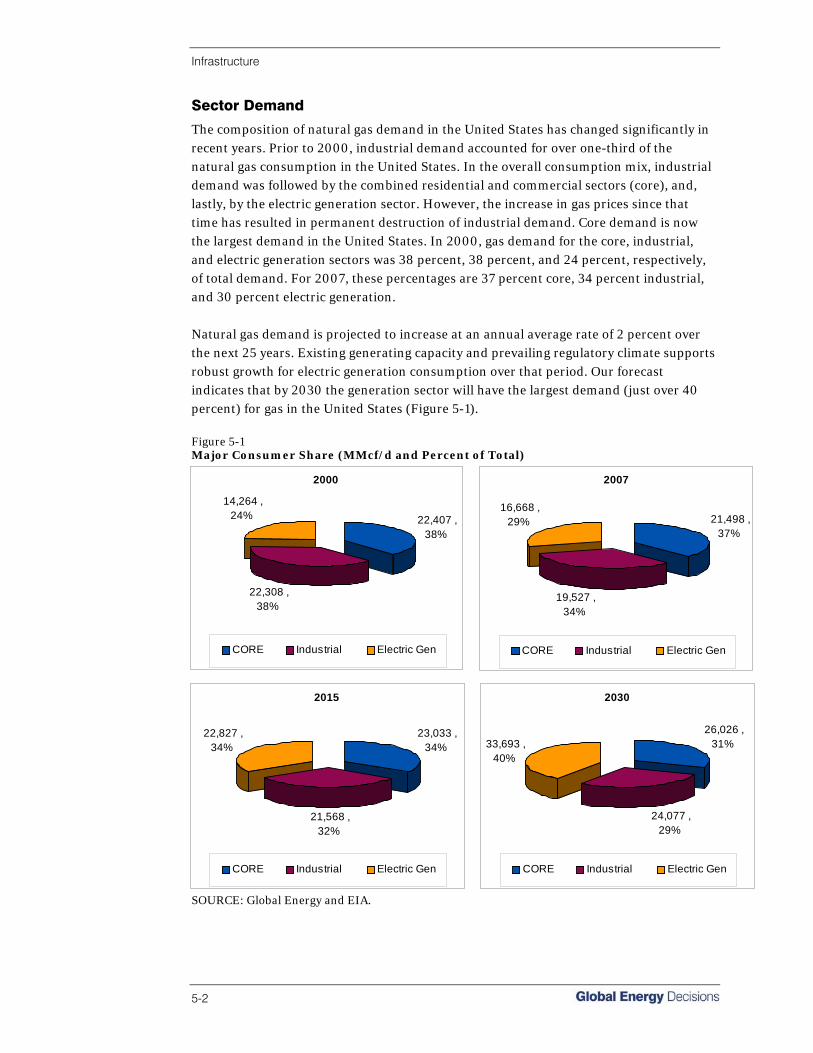
Infrastructure
5-2
Sector Demand
The composition of natural gas demand in the United States has changed significantly in recent years. Prior to 2000, industrial demand accounted for over one-third of the natural gas consumption in the United States. In the overall consumption mix, industrial demand was followed by the combined residential and commercial sectors (core), and, lastly, by the electric generation sector. However, the increase in gas prices since that time has resulted in permanent destruction of industrial demand. Core demand is now the largest demand in the United States. In 2000, gas demand for the core, industrial, and electric generation sectors was 38 percent, 38 percent, and 24 percent, respectively, of total demand. For 2007, these percentages are 37 percent core, 34 percent industrial, and 30 percent electric generation. Natural gas demand is projected to increase at an annual average rate of 2 percent over the next 25 years. Existing generating capacity and prevailing regulatory climate supports robust growth for electric generation consumption over that period. Our forecast indicates that by 2030 the generation sector will have the largest demand (just over 40 percent) for gas in the United States (Figure 5-1). Figure 5-1 Major Consumer Share (MMcf/d and Percent of Total)
2000
22,407 , 38%
22,308 , 38%
14,264 , 24%
CORE Industrial Electric Gen
2007
21,498 , 37%
19,527 , 34%
16,668 , 29%
CORE Industrial Electric Gen
2015
23,033 , 34%
21,568 , 32%
22,827 , 34%
CORE Industrial Electric Gen
2030
26,026 , 31%
24,077 , 29%
33,693 , 40%
CORE Industrial Electric Gen
SOURCE: Global Energy and EIA.
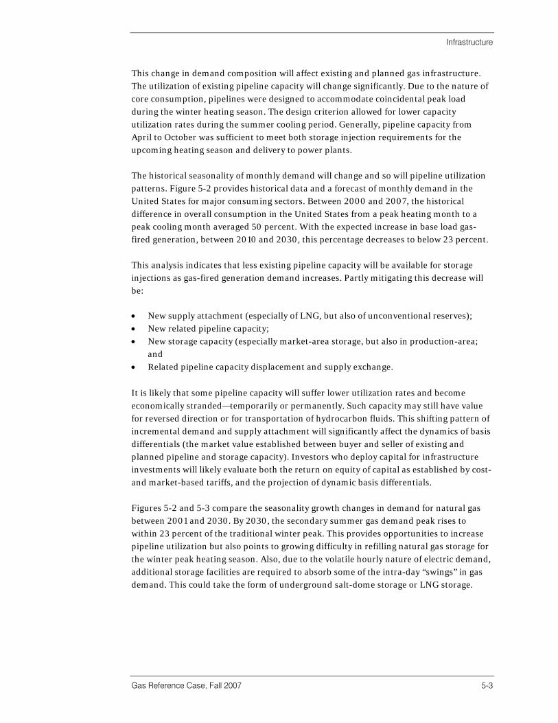
Infrastructure
Gas Reference Case, Fall 2007 5-3
This change in demand composition will affect existing and planned gas infrastructure. The utilization of existing pipeline capacity will change significantly. Due to the nature of core consumption, pipelines were designed to accommodate coincidental peak load during the winter heating season. The design criterion allowed for lower capacity utilization rates during the summer cooling period. Generally, pipeline capacity from April to October was sufficient to meet both storage injection requirements for the upcoming heating season and delivery to power plants. The historical seasonality of monthly demand will change and so will pipeline utilization patterns. Figure 5-2 provides historical data and a forecast of monthly demand in the United States for major consuming sectors. Between 2000 and 2007, the historical difference in overall consumption in the United States from a peak heating month to a peak cooling month averaged 50 percent. With the expected increase in base load gas-fired generation, between 2010 and 2030, this percentage decreases to below 23 percent. This analysis indicates that less existing pipeline capacity will be available for storage injections as gas-fired generation demand increases. Partly mitigating this decrease will be: • New supply attachment (especially of LNG, but also of unconventional reserves); • New related pipeline capacity; • New storage capacity (especially market-area storage, but also in production-area;
and • Related pipeline capacity displacement and supply exchange.
It is likely that some pipeline capacity will suffer lower utilization rates and become economically stranded—temporarily or permanently. Such capacity may still have value for reversed direction or for transportation of hydrocarbon fluids. This shifting pattern of incremental demand and supply attachment will significantly affect the dynamics of basis differentials (the market value established between buyer and seller of existing and planned pipeline and storage capacity). Investors who deploy capital for infrastructure investments will likely evaluate both the return on equity of capital as established by cost- and market-based tariffs, and the projection of dynamic basis differentials. Figures 5-2 and 5-3 compare the seasonality growth changes in demand for natural gas between 2001 and 2030. By 2030, the secondary summer gas demand peak rises to within 23 percent of the traditional winter peak. This provides opportunities to increase pipeline utilization but also points to growing difficulty in refilling natural gas storage for the winter peak heating season. Also, due to the volatile hourly nature of electric demand, additional storage facilities are required to absorb some of the intra-day “swings” in gas demand. This could take the form of underground salt-dome storage or LNG storage.
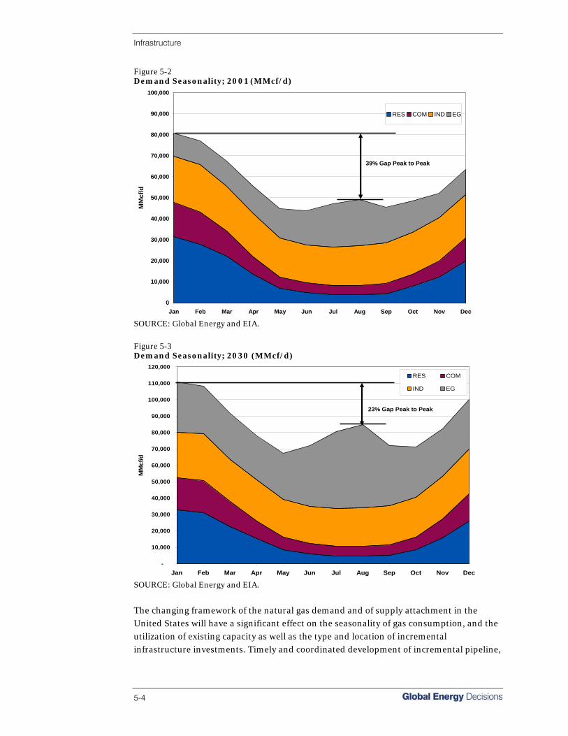
Infrastructure
5-4
Figure 5-2 Demand Seasonality; 2001 (MMcf/d)
0
10,000
20,000
30,000
40,000
50,000
60,000
70,000
80,000
90,000
100,000
Jan Feb Mar Apr May Jun Jul Aug Sep Oct Nov Dec
MM
cf/d
RES COM IND EG
39% Gap Peak to Peak
SOURCE: Global Energy and EIA.
Figure 5-3 Demand Seasonality; 2030 (MMcf/d)
-
10,000
20,000
30,000
40,000
50,000
60,000
70,000
80,000
90,000
100,000
110,000
120,000
Jan Feb Mar Apr May Jun Jul Aug Sep Oct Nov Dec
MM
cf/d
RES COM
IND EG
23% Gap Peak to Peak
SOURCE: Global Energy and EIA.
The changing framework of the natural gas demand and of supply attachment in the United States will have a significant effect on the seasonality of gas consumption, and the utilization of existing capacity as well as the type and location of incremental infrastructure investments. Timely and coordinated development of incremental pipeline,
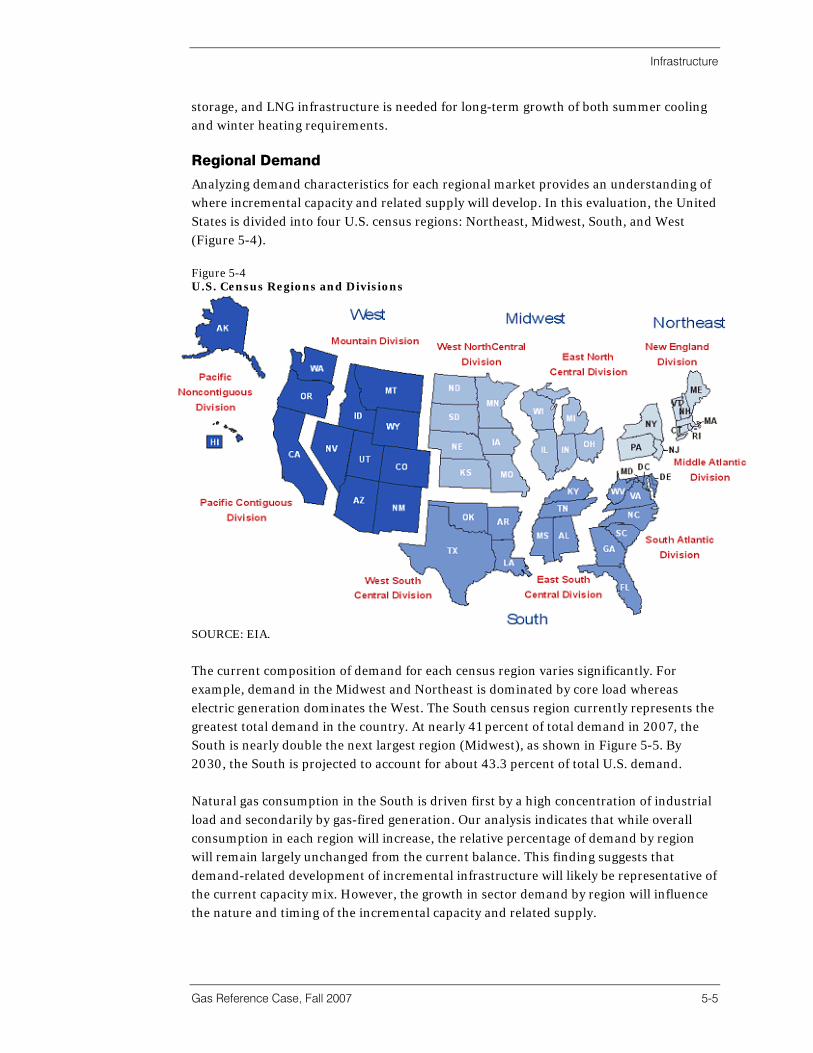
Infrastructure
Gas Reference Case, Fall 2007 5-5
storage, and LNG infrastructure is needed for long-term growth of both summer cooling and winter heating requirements. Regional Demand
Analyzing demand characteristics for each regional market provides an understanding of where incremental capacity and related supply will develop. In this evaluation, the United States is divided into four U.S. census regions: Northeast, Midwest, South, and West (Figure 5-4). Figure 5-4 U.S. Census Regions and Divisions
SOURCE: EIA.
The current composition of demand for each census region varies significantly. For example, demand in the Midwest and Northeast is dominated by core load whereas electric generation dominates the West. The South census region currently represents the greatest total demand in the country. At nearly 41 percent of total demand in 2007, the South is nearly double the next largest region (Midwest), as shown in Figure 5-5. By 2030, the South is projected to account for about 43.3 percent of total U.S. demand. Natural gas consumption in the South is driven first by a high concentration of industrial load and secondarily by gas-fired generation. Our analysis indicates that while overall consumption in each region will increase, the relative percentage of demand by region will remain largely unchanged from the current balance. This finding suggests that demand-related development of incremental infrastructure will likely be representative of the current capacity mix. However, the growth in sector demand by region will influence the nature and timing of the incremental capacity and related supply.
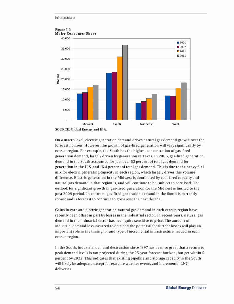
Infrastructure
5-6
Figure 5-5 Major Consumer Share
-
5,000
10,000
15,000
20,000
25,000
30,000
35,000
40,000
Midwest South Northeast West
MM
cf/d
2001200720212031
SOURCE: Global Energy and EIA.
On a macro level, electric generation demand drives natural gas demand growth over the forecast horizon. However, the growth of gas-fired generation will vary significantly by census region. For example, the South has the highest concentration of gas-fired generation demand, largely driven by generation in Texas. In 2006, gas-fired generation demand in the South accounted for just over 63 percent of total gas demand for generation in the U.S. and 16.4 percent of total gas demand. This is due to the heavy fuel mix for electric generating capacity in each region, which largely drives this volume difference. Electric generation in the Midwest is dominated by coal-fired capacity and natural gas demand in that region is, and will continue to be, subject to core load. The outlook for significant growth in gas-fired generation for the Midwest is limited to the post 2009 period. In contrast, gas-fired generation demand in the South is currently robust and is forecast to continue to grow over the next decade. Gains in core and electric generation natural gas demand in each census region have recently been offset in part by losses in the industrial sector. In recent years, natural gas demand in the industrial sector has been quite sensitive to price. The amount of industrial demand loss incurred to date and the potential for further losses will play an important role in the timing for and type of incremental infrastructure needed in each census region. In the South, industrial demand destruction since 1997 has been so great that a return to peak demand levels is not projected during the 25-year forecast horizon, but get within 5 percent by 2032. This indicates that existing pipeline and storage capacity in the South will likely be adequate except for extreme weather events and incremental LNG deliveries.
Infrastructure
Gas Reference Case, Fall 2007 5-7
This conclusion is similar for overall demand in the Midwest. On the other hand, natural gas demand in the Northeast and West is forecast to meet or exceed historical peaks by 2007, suggesting that existing infrastructure is likely to be insufficient, which may lead to increased price volatility for those regions during the forecast horizon. Ultimately, incremental infrastructure requirements will vary significantly by census region. Demand-driven infrastructure development will be dependent on economic variables such as demand elasticity, population growth, and the overall performance of the U.S. and regional economies. Our analysis suggests that although demand sectors may shift intra-regionally, the majority of natural gas demand will remain concentrated in the South with most demand-influenced infrastructure development. Demand dynamics will also influence the timing and nature of new supply, and its attachment strategy to existing and new pipeline and storage capacity.
Supply Influences The nature of incremental demand growth requires the timely development of additional domestic reserves and natural gas imports—both long-haul Arctic gas and LNG. In 2006, domestic gas production was adequate to supply approximately 84 percent of the total gas consumed in the United States. This indigenous gas was largely from conventional reservoirs not associated with oil, but included increasing volumes of unconventional gas from coalbeds and tight sandstone and shales. Gas associated with Lower 48-state oil production provided approximately 13 percent of the gas supply and its share is expected to increase with sustainable high oil prices. The balance of supply was largely pipeline imports from Canada and minor supplies (2.4 percent in 2006) of LNG. With the expectation for growing demand across North America and the outlook for static to declining production rates from conventional reservoirs, new supply sources both domestic and imported will be increasingly utilized to meet expected market growth. The expansion and increased utilization of new supply sources will largely drive the development of pipeline, storage, and LNG infrastructure over the forecast horizon and will be coordinated with intra-regional shifts in sector demand. Supply-driven pipeline and storage development will be centered on incremental production growth in the Rocky Mountains, eastern Texas, deep-water Gulf of Mexico, Arctic gas, and increased LNG imports. Lower 48 Supply Development
Over the last few years, various expansions to existing pipeline corridors and investments in expansion capacity have been made to accommodate Rocky Mountain supply growth. The recent wave of Rockies-focused infrastructure development was kicked off by Kern River Gas Transmission’s 2003 expansion. The 2003 Kern River expansion more than doubled the pipeline’s Wyoming-to-California corridor to 1.73 Bcf/d. More recently, new construction and pipeline proposals have been centered on takeaway capacity to lucrative Eastern and Midwestern markets. This change in focus has been bolstered by the expectation for competition from LNG deliveries at the California border and the prospect for enhanced commodity value in premium Eastern markets.
Infrastructure
5-8
EnCana’s recent Entrega proposal is a good example of this changing dynamic. The Entrega project is projected to move 1.3 Bcf/d from the Piceance Basin of northwestern Colorado through the southern Wyoming supply regions to the Cheyenne hub at the Wyoming/Colorado border where a number of existing and proposed eastbound pipelines converge. In addition, Kinder Morgan and Sempra Energy Partners are planning to construct a 1.8 Bcf/d, 1,323-mile pipeline from the Cheyenne hub to the Ohio/ Pennsylvania border by 2009. They are currently seeking interest in its extension to the New York citygate. El Paso also has a similar proposal (the Continental Connector pipeline) to deliver Rocky and Mid-Continent gas to their long-haul pipelines in northern Louisiana for redelivery to Eastern markets by late 2009. Our production forecast calls for an incremental 1.5 Bcf/d of gas to be delivered out of the Rockies starting in January 2008 and reach 2 Bcf/d by 2012. This expected increase in supply deliverability more than justifies some combination of these proposals. Production in the northeastern and southern parts of Texas has also been on the rise, providing approximately 3.0 Bcf/d of increased production between 1995 and 2005. In fact, the East Texas Basin is now the largest producer in Texas, bolstered by production from unconventional tight reservoirs of the Bossier Sand and Barnett Shale plays. The outlook for production growth in East Texas has recently supported a number of pipeline expansion proposals. To transport gas out of the prolific East Texas region, Gulf South Pipeline, Texas Gas Transmission, and Energy Transfer Partners have joined to build two new pipelines that will interconnect with existing pipeline systems in East Texas near the Carthage hub. The eventual construction of the new pipelines is contingent on many factors, including the completion of the supply development process, as well as gaining customer commitments and regulatory approvals. Gulf South has proposed a 1 Bcf/d, 36-inch pipe that will flow from an interconnect with Energy Transfer’s pipes in Carthage to the Gulf South mainline in Louisiana and Mississippi and also to Texas Gas Transmission’s mainline in Louisiana. Gulf South currently has their 1.7 Bcf/d East Texas to Mississippi Expansion Project under construction to running 42-inch and 36-inch pipe to MS, and scheduled to be completed later this year. The other pipeline proposal is from Energy Transfer to build a 36-inch pipe reaching from its Texoma Pipeline to Carthage. These new pipelines, in conjunction with existing infrastructure, will provide transportation access from the major supply basins in Texas and bring gas to the Henry Hub and various interconnects with Florida Gas Transmission, Transco, and Texas Eastern. Natural Gas Pipeline of America (NGPL) is testing the market for an expansion on their Amarillo to Gulf Coast (AG) line of an estimated 230 MMcf/d. This expansion is in addition to the Crosstex proposal to build a 250 MMcf/d header, which connects with NGPL, Houston Pipeline, and Kinder Morgan Interstate Pipeline.
Infrastructure
Gas Reference Case, Fall 2007 5-9
A similar feature of the eastbound Rockies proposals and the East Texas takeaway pipes is that they all utilize existing pipeline infrastructure and right-of-ways to access Eastern markets. With production projected to slowly decline in the Mid-Continent and Gulf Coast, the expectation is that sufficient pipeline infrastructure will be available to serve the Midwest and Eastern markets. The East Texas expansions should have an advantage because of the short distance to access the major long-haul pipelines that serve the Northeast. In contrast, the Rockies pipelines cross existing pipelines already serving the Midwest markets that receive supply from Canada, the Mid-Continent, the Gulf Coast (including East Texas and offshore production), and the expected increase in LNG deliveries. Ultimately, additional pipeline expansion of the Midwest-to-Northeast corridor will be required to redeliver Rocky Mountain and Arctic gas to Eastern markets. A recent addition to the Midwest-to-Northeast corridor, Vector Pipeline, has realized very high utilization rates. In fact, Vector has contributed to a decrease in net imports from Canada as Midwest gas has moved through the Dawn, Ontario, hub to access northeastern markets. Arctic Gas
U.S. and Canadian frontier gas will be very important to North American gas supplies over the next few decades. On Alaska’s North Slope, the National Petroleum Reserve Area (NPRA) is already being developed through a leasing and exploration program. Current estimates by the Energy Information Agency and U.S. Geological Survey for North American Arctic gas include: • Alaska
o Prudhoe Bay: 30 Tcf o Point Thompson: 8 Tcf
• Canadian Mackenzie Delta region: 6 Tcf • Total: 44 Tcf Prudhoe Bay gas is currently being injected for secondary oil recovery, as mandated by the Alaskan State Department of Revenue to maximize hydrocarbon recovery and royalty income. The Point Thompson field is a condensate field (up to 15 percent NGL), which its operator (ExxonMobil) claims cannot be economically extracted unless the NGL-stripped gas has a pipeline to market. The State of Alaska disagrees and has recently declared the leases in default and eligible for new round of lease bidding. Predictably, the producers have sought judicial relief. The proved gas in the Mackenzie Delta region is in three fields (Tagula, Parsons Lake, and Niglintgak) and is largely non-associated with oil or condensate reservoirs. It too is economically stranded without a pipeline for delivery to market hubs (AECO and Joliet). In addition to the approximately 45 Tcf of proved Arctic gas (85 percent in Alaska, 15 percent in Canada), gas also occurs in the Alaskan National Petroleum Reserve Area (NPRA). EIA reported that the NPRA contains approximately 50 to 100 Tcf of technically
Infrastructure
5-10
recoverable gas. Approximately 85 percent of this gas is not associated with oil or condensate reservoirs. The U.S. Geological Survey also reports that approximately 65 Tcf of risk-weighted undiscovered gas resources exist in the Alaskan North Slope and approximately 30 Tcf in the Beaufort Sea region north of Mackenzie Bay, largely in the Northwest Territories of Canada. The North American Arctic is therefore now estimated to contain: • 38 Tcf of proved Alaskan reserves; • 6 Tcf of proved Mackenzie Delta reserves; • 115-165 Tcf of unproved reserves in the Alaska North Slope;
o 35 to 50 percent technically recoverable, plus; o 55 to 40 percent likely undiscovered resources;
• 30 Tcf of unproved reserves in the Beaufort Sea region of Canada. • Total: 190-240 Tcf (proved and unproved). The economic recovery of these resources is wholly dependent on the deployment of an extremely large amount of development capital. The investment in infrastructure to develop a likely 145 to 195 Tcf of Arctic gas is very large, in the tens of billions of dollars. This potential supply could satisfy seven to ten years of total U.S. demand without contribution from any other North America indigenous source. The availability of such an investment is largely dependent on the projected wellhead net-back price after the in-service dates of the Alaska Stranded Gas Pipeline (ASGR) and Mackenzie Delta Pipeline (MDP). The economic feasibility of a commercial net-back commodity price sufficient to justify Arctic pipelines such as ASGP and MDP is dependent on several key parameters: • Stable governmental fiscal policy, including future taxation on oil and condensate
production. This is especially important to development of marginally economic satellite fields. Such policy also includes the level of governmental support for aboriginal group participation and other forms of compensation.
• The cost of pipeline construction prior to start-up, and its design as either an NGL-rich bullet line similar to the Alliance Pipeline, or a dry-gas line with potential for lateral delivery for local usage along the right-of way. The normalization of current hyper-inflation cost will be needed in order to establish economic feasibility prior to the start-up date for construction.
• A daily through-put rate and level of shipper commitment to pay for 15 years or more of demand charges for leased capacity. Shipper’s risks include stranded capacity due to competition from LNG in their downstream coastal markets, and due to subsequent regulatory cost disallowance.
• The daily production rate of existing and new satellite fields and the ability to gather and aggregate these smaller fields in order to share infrastructure capacity as primary fields deplete. Prudhoe Bay’s initial daily rate is reported between 4.5 and 6.5 Bcf/d and Mackenzie Delta’s between 1.2 and 2.4 Bcf/d (excluding fuel retention). The 145-195 Tcf of likely non-proved reserves in NPRA and elsewhere on the North Slop of Alaska could support the ASGP for an additional 20 to 30 years after the production
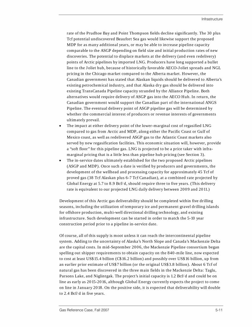
Infrastructure
Gas Reference Case, Fall 2007 5-11
rate of the Prudhoe Bay and Point Thompson fields decline significantly. The 30 plus Tcf potential undiscovered Beaufort Sea gas would likewise support the proposed MDP for as many additional years, or may be able to increase pipeline capacity comparable to the ASGP depending on field size and initial production rates of new discoveries. The potential to displace markets at the delivery (and even redelivery) points of Arctic pipelines by imported LNG. Producers have long supported a bullet line to the Joliet hub, because of historically favorable AECO-Joliet spreads and NGL pricing in the Chicago market compared to the Alberta market. However, the Canadian government has stated that Alaskan liquids should be delivered to Alberta’s existing petrochemical industry, and that Alaska dry gas should be delivered into existing TransCanada Pipeline capacity stranded by the Alliance Pipeline. Both alternatives would require delivery of ASGP gas into the AECO Hub. In return, the Canadian government would support the Canadian part of the international ANGS Pipeline. The eventual delivery point of ASGP pipeline gas will be determined by whether the commercial interest of producers or revenue interests of governments ultimately prevail.
• The impact at either delivery point of the lower-marginal cost of regasified LNG compared to gas from Arctic and MDP, along either the Pacific Coast or Gulf of Mexico coast, as well as redelivered ASGP gas to the Atlantic Coast markets also served by new regasification facilities. This economic situation will, however, provide a “soft floor” for this pipeline gas. LNG is projected to be a price taker with infra-marginal pricing that is a little less than pipeline hub pricing (see Section 3).
• The in-service dates ultimately established for the two proposed Arctic pipelines (ASGP and MDP). Once such a date is verified by producers and governments, the development of the wellhead and processing capacity for approximately 45 Tcf of proved gas (38 Tcf Alaskan plus 6-7 Tcf Canadian), at a combined rate projected by Global Energy at 5.7 to 8.9 Bcf/d, should require three to five years. (This delivery rate is equivalent to our projected LNG daily delivery between 2009 and 2011.)
Development of this Arctic gas deliverability should be completed within five drilling seasons, including the utilization of temporary ice and permanent gravel drilling islands for offshore production, multi-well directional drilling technology, and existing infrastructure. Such development can be started in order to match the 5-10 year construction period prior to a pipeline in-service date. Of course, all of this supply is moot unless it can reach the intercontinental pipeline system. Adding to the uncertainty of Alaska’s North Slope and Canada’s Mackenzie Delta are the capital costs. In mid-September 2006, the Mackenzie Pipeline consortium began spelling out shipper requirements to obtain capacity on the 840-mile line, now expected to cost at least US$15.4 billion (C$16.2 billion) and possibly over US$16 billion, up from an earlier prior estimate of US$7 billion (or the original US$3.8 billion). About 6 Tcf of natural gas has been discovered in the three main fields in the Mackenzie Delta: Taglu, Parsons Lake, and Niglintgak. The project’s initial capacity is 1.2 Bcf/d and could be on line as early as 2015-2016, although Global Energy currently expects the project to come on line in January 2018. On the positive side, it is expected that deliverability will double to 2.4 Bcf/d in five years.
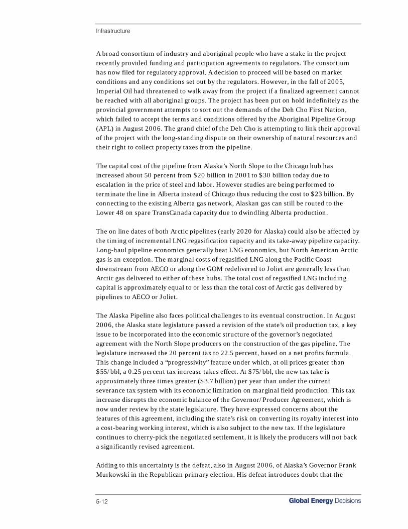
Infrastructure
5-12
A broad consortium of industry and aboriginal people who have a stake in the project recently provided funding and participation agreements to regulators. The consortium has now filed for regulatory approval. A decision to proceed will be based on market conditions and any conditions set out by the regulators. However, in the fall of 2005, Imperial Oil had threatened to walk away from the project if a finalized agreement cannot be reached with all aboriginal groups. The project has been put on hold indefinitely as the provincial government attempts to sort out the demands of the Deh Cho First Nation, which failed to accept the terms and conditions offered by the Aboriginal Pipeline Group (APL) in August 2006. The grand chief of the Deh Cho is attempting to link their approval of the project with the long-standing dispute on their ownership of natural resources and their right to collect property taxes from the pipeline. The capital cost of the pipeline from Alaska’s North Slope to the Chicago hub has increased about 50 percent from $20 billion in 2001 to $30 billion today due to escalation in the price of steel and labor. However studies are being performed to terminate the line in Alberta instead of Chicago thus reducing the cost to $23 billion. By connecting to the existing Alberta gas network, Alaskan gas can still be routed to the Lower 48 on spare TransCanada capacity due to dwindling Alberta production. The on line dates of both Arctic pipelines (early 2020 for Alaska) could also be affected by the timing of incremental LNG regasification capacity and its take-away pipeline capacity. Long-haul pipeline economics generally beat LNG economics, but North American Arctic gas is an exception. The marginal costs of regasified LNG along the Pacific Coast downstream from AECO or along the GOM redelivered to Joliet are generally less than Arctic gas delivered to either of these hubs. The total cost of regasified LNG including capital is approximately equal to or less than the total cost of Arctic gas delivered by pipelines to AECO or Joliet. The Alaska Pipeline also faces political challenges to its eventual construction. In August 2006, the Alaska state legislature passed a revision of the state’s oil production tax, a key issue to be incorporated into the economic structure of the governor’s negotiated agreement with the North Slope producers on the construction of the gas pipeline. The legislature increased the 20 percent tax to 22.5 percent, based on a net profits formula. This change included a “progressivity” feature under which, at oil prices greater than $55/bbl, a 0.25 percent tax increase takes effect. At $75/bbl, the new tax take is approximately three times greater ($3.7 billion) per year than under the current severance tax system with its economic limitation on marginal field production. This tax increase disrupts the economic balance of the Governor/Producer Agreement, which is now under review by the state legislature. They have expressed concerns about the features of this agreement, including the state’s risk on converting its royalty interest into a cost-bearing working interest, which is also subject to the new tax. If the legislature continues to cherry-pick the negotiated settlement, it is likely the producers will not back a significantly revised agreement. Adding to this uncertainty is the defeat, also in August 2006, of Alaska’s Governor Frank Murkowski in the Republican primary election. His defeat introduces doubt that the

Infrastructure
Gas Reference Case, Fall 2007 5-13
legislature will pass the balance of his negotiated agreement without additional changes. Sarah Palin, the Republican primary victor, has stated she supports many of the concerns expressed by the state House, winning in November and taking office in December 2006. Any additional revision might delay the construction of the Alaska Pipeline; however, in May 2007 the Alaska Gasline Inducement Act (AGIA) was enacted by the legislature outlining guidelines for inducing construction of the pipeline. This includes state matching contributions of up to $500 million for expenditures toward the planning and construction of an Alaskan gas pipeline project and other state administrative benefits. Imported Natural Gas and LNG
To fill the need for LNG to replace declining domestic production, new pipelines and storage facilities will be needed near LNG terminals. But where will those terminals be? Currently, onshore and offshore regasification facilities generally face fierce opposition to their construction from local residents with environmental, safety, or terrorism concerns. This opposition varies from state to state and city to city. Some areas welcome the economic benefits of industry and pose virtually no opposition. Others take a not-in-my-backyard attitude and dispute all the merits of having an LNG facility in their community. How these concerns are resolved will determine what types of new LNG facilities are built, where they are located, and the needed take-away transportation capacity. At present, new facilities often face the least resistance in areas with an already established strong energy development and transportation infrastructure, such as the Gulf Coasts of Texas and Louisiana. The Gulf of Mexico has additional advantages for LNG terminal development: • Excess capacity on many pipelines, the result of declining conventional production; • Access to gas processing facilities to adjust LNG compositions; • Access to low-deliverability storage for regasified LNG; and • A sympathetic public, along with public officials familiar with energy infrastructure
and appreciative of an increased tax base.
It is reasonable to expect a significant portion of the new LNG development to occur in the Gulf of Mexico area. These new LNG facilities will require new pipeline infrastructure, especially short-haul laterals and interconnection headers. Sempra Energy’s Port Arthur LNG proposal provides an example. Along with the approval they are seeking from FERC for the LNG facility itself, Sempra has also requested approval to build a 70-mile, 36-inch pipeline that will interconnect with Transcontinental Gas Pipeline. In addition, Southern Natural Gas (SNG) has proposed a 165-mile, 1.1 Bcf/d Elba Express Pipeline from the Elba Island LNG facility to markets in Georgia to interconnect with pipelines to the southeastern and Eastern markets. SNG’s 165-mile proposed Cypress Pipeline will connect in Georgia and terminate in Clay County, Florida, at an interconnection with the FGT pipeline system. The in service dates for these two projects are mid-2011 and late-2007, respectively. The expansion of the Cove Point LNG facility is the impetus for the proposed Sentinel Expansion (0.2-0.3 Bcf/d) from Cove Point to the Leidy hub, and to storage facilities in
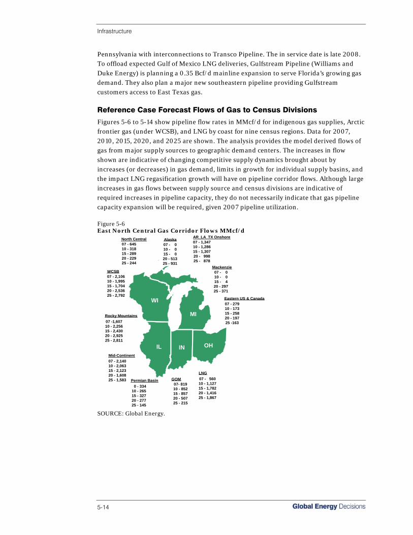
Infrastructure
5-14
Pennsylvania with interconnections to Transco Pipeline. The in service date is late 2008. To offload expected Gulf of Mexico LNG deliveries, Gulfstream Pipeline (Williams and Duke Energy) is planning a 0.35 Bcf/d mainline expansion to serve Florida’s growing gas demand. They also plan a major new southeastern pipeline providing Gulfstream customers access to East Texas gas. Reference Case Forecast Flows of Gas to Census Divisions
Figures 5-6 to 5-14 show pipeline flow rates in MMcf/d for indigenous gas supplies, Arctic frontier gas (under WCSB), and LNG by coast for nine census regions. Data for 2007, 2010, 2015, 2020, and 2025 are shown. The analysis provides the model derived flows of gas from major supply sources to geographic demand centers. The increases in flow shown are indicative of changing competitive supply dynamics brought about by increases (or decreases) in gas demand, limits in growth for individual supply basins, and the impact LNG regasification growth will have on pipeline corridor flows. Although large increases in gas flows between supply source and census divisions are indicative of required increases in pipeline capacity, they do not necessarily indicate that gas pipeline capacity expansion will be required, given 2007 pipeline utilization. Figure 5-6 East North Central Gas Corridor Flows MMcf/d
WI
IN
MI
IL OH
07 - 2,14010 - 2,06315 - 2,12320 - 1,60825 - 1,583
Mid-Continent
07 - 2,10610 - 1,99515 - 1,70420 - 2,53625 - 2,792
WCSB
07 -1,60710 - 2,25615 - 2,43020 - 2,92525 - 2,811
Rocky Mountains
07 - 27910 - 17315 - 25820 - 19725 -163
Eastern US & Canada
07- 81910 - 85215 - 85720 - 50725 - 215
GOM 07 - 56010 - 1,12715 - 1,78220 - 1,41625 - 1,867
LNG
0 - 33410 - 26515 - 32720 - 27725 - 145
Permian Basin
07 - 64510 - 31815 - 28920 - 22925 - 244
North Central07 - 010 - 015 - 020 - 51325 - 931
Alaska 07 - 1,34710 - 1,28615 - 1,30720 - 99825 - 878
AR_LA_TX Onshore
07 - 010 - 015 - 420 - 29725 - 371
Mackenzie
SOURCE: Global Energy.

Infrastructure
Gas Reference Case, Fall 2007 5-15
Figure 5-7 East South Central Gas Corridor Flows MMcf/d
MS
TN
KY
AL
AR-LA-TX Onshore07 - 1,55910 - 1,65115 - 1,82520 - 2,01125 - 2,082
LNG07 - 8910 - 20215 - 51020 - 70125 - 1,142
Eastern US & Canada07 - 13110 - 12815 - 11420 - 11725 - 115
GOM07 - 1,11610 - 1,10415 - 1,16920 - 1,15725 - 1,196
SOURCE: Global Energy.
Figure 5-8 Middle Atlantic Gas Corridor Flows MMcf/d
NY
NJPA
07 - 9910 - 2115 - 1720 - 2725 - 35
Mid-Continent
07 - 7510 - 32315 - 32520 - 38425 - 482
Rocky Mountains
07 - 1,10410 - 1,14315 - 1,09620 - 1,04725 - 969
WCSB
07 - 010 - 015 - 020 - 29225 - 474
Alaska
07 - 1,27110 - 1,11415 - 1,03920 - 99825 - 1,047
Eastern US & Canada
07 - 2,42710 - 2,14115 - 1,61920 - 1,25225 - 1,169
GOM
07 - 15110 - 85815 - 2,00820 - 2,27925 - 2,716
LNG
07 - 1,74510 - 1,33715 - 1,11120 - 1,03325 - 1,046
AR-LA-TX Onshore
07 - 010 - 015 - 120 - 10125 - 130
MacKenzie
SOURCE: Global Energy.
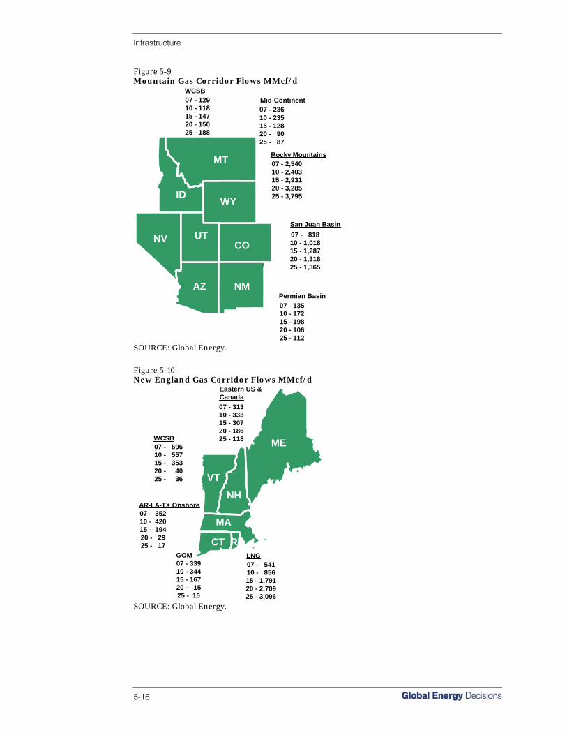
Infrastructure
5-16
Figure 5-9 Mountain Gas Corridor Flows MMcf/d
MT
ID
NV UT
WY
CO
AZ NM
07 - 23610 - 23515 - 12820 - 9025 - 87
Mid-Continent
07 - 13510 - 17215 - 19820 - 10625 - 112
Permian Basin
07 - 2,54010 - 2,40315 - 2,93120 - 3,28525 - 3,795
Rocky Mountains
07 - 81810 - 1,01815 - 1,28720 - 1,31825 - 1,365
San Juan Basin
07 - 12910 - 11815 - 14720 - 15025 - 188
WCSB
SOURCE: Global Energy.
Figure 5-10 New England Gas Corridor Flows MMcf/d
ME
RI
NH
VT
MA
CT
07 - 69610 - 55715 - 35320 - 4025 - 36
WCSB
07 - 54110 - 85615 - 1,79120 - 2,70925 - 3,096
LNG
07 - 35210 - 42015 - 19420 - 2925 - 17
AR-LA-TX Onshore
07 - 33910 - 34415 - 16720 - 1525 - 15
GOM
07 - 31310 - 33315 - 30720 - 18625 - 118
Eastern US &Canada
SOURCE: Global Energy.
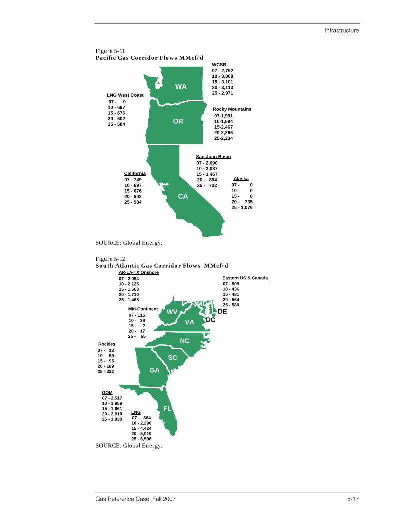
Infrastructure
Gas Reference Case, Fall 2007 5-17
Figure 5-11 Pacific Gas Corridor Flows MMcf/d
WA
CA
OR
WCSB07 - 2,79210 - 3,06815 - 3,10120 - 3,11325 - 2,971
Rocky Mountains07-1,99110-1,69415-2,46720-2,26625-2,234
San Juan Basin07 - 2,09010 - 2,08715 - 1,46720 - 89425 - 732
Alaska07 - 010 - 015 - 020 - 73525 - 1,076
California07 - 74910 - 69715 - 67620 - 60225 - 584
LNG West Coast 07 - 010 - 69715 - 67620 - 60225 - 584
SOURCE: Global Energy.
Figure 5-12 South Atlantic Gas Corridor Flows MMcf/d
FL
SC
GA
NC
VAWV
MDDE
DC
Mid-Continent07 - 11510 - 3915 - 220 - 1725 - 55
GOM07 - 2,51710 - 1,98915 - 1,66120 - 2,01025 - 1,830
07 - 50910 - 43615 - 48120 - 56425 - 580
Eastern US & Canada
LNG07 - 86410 - 2,29615 - 4,42420 - 5,01025 - 6,596
Rockies07 - 1310 - 9915 - 9520 - 18925 - 322
AR-LA-TX Onshore07 - 2,09410 - 2,12515 - 1,66320 - 1,71025 - 1,468
SOURCE: Global Energy.
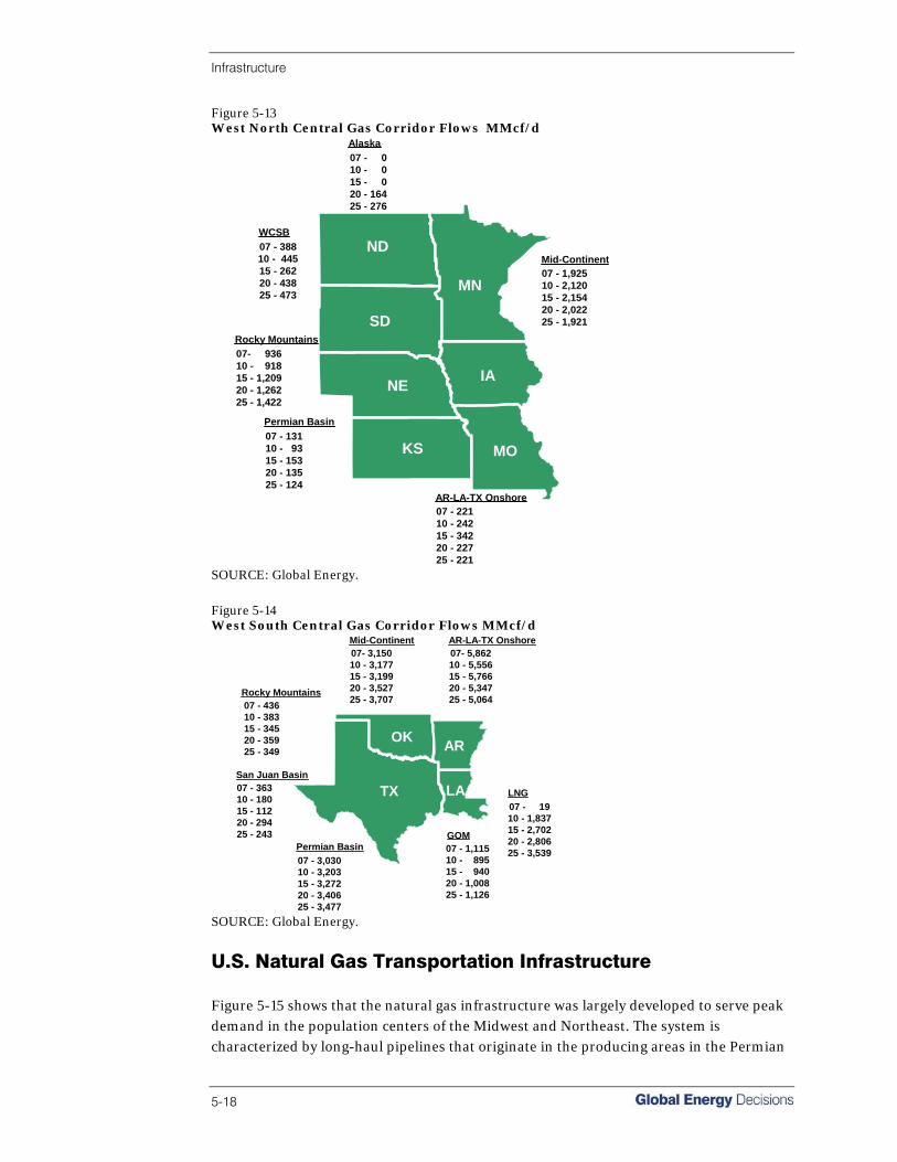
Infrastructure
5-18
Figure 5-13 West North Central Gas Corridor Flows MMcf/d
ND
SD
MN
NE
KS
IA
MO
07 - 1,92510 - 2,12015 - 2,15420 - 2,02225 - 1,921
Mid-Continent
WCSB07 - 38810 - 44515 - 26220 - 43825 - 473
07 - 13110 - 9315 - 15320 - 13525 - 124
Permian Basin
07 - 22110 - 24215 - 34220 - 22725 - 221
AR-LA-TX Onshore
07- 93610 - 91815 - 1,20920 - 1,26225 - 1,422
Rocky Mountains
Alaska07 - 010 - 015 - 020 - 16425 - 276
SOURCE: Global Energy.
Figure 5-14 West South Central Gas Corridor Flows MMcf/d
TX
OK AR
LA
Mid-Continent07- 3,15010 - 3,17715 - 3,19920 - 3,52725 - 3,707
GOM07 - 1,11510 - 89515 - 94020 - 1,00825 - 1,126
San Juan Basin07 - 36310 - 18015 - 11220 - 29425 - 243
LNG07 - 1910 - 1,83715 - 2,70220 - 2,80625 - 3,539
Rocky Mountains07 - 43610 - 38315 - 34520 - 35925 - 349
07 - 3,03010 - 3,20315 - 3,27220 - 3,40625 - 3,477
Permian Basin
AR-LA-TX Onshore07- 5,86210 - 5,55615 - 5,76620 - 5,34725 - 5,064
SOURCE: Global Energy.
U.S. Natural Gas Transportation Infrastructure Figure 5-15 shows that the natural gas infrastructure was largely developed to serve peak demand in the population centers of the Midwest and Northeast. The system is characterized by long-haul pipelines that originate in the producing areas in the Permian

Infrastructure
Gas Reference Case, Fall 2007 5-19
Basin, Mid-Continent, and Gulf Coast, and that redeliver gas to high-demand states such as Illinois, Michigan, Ohio, Pennsylvania, and New York. This natural gas infrastructure also developed production area storage to support peak load delivery to these regional demand centers. Figure 5-15 Natural Gas Infrastructure in North America
Natural Gas Pipelines
Storage Facilities
Supply Basins
Natural Gas Pipelines
Storage Facilities
Supply Basins
Natural Gas Pipelines
Storage Facilities
Supply Basins
SOURCE: Global Energy.
An examination of supply and demand both nationally and regionally provides a framework for the changes likely to occur to the North American natural gas transportation grid. In 2004, according to the American Gas Association, there were 2.2 million miles of natural gas pipeline in the United States. Of the 2.2 million pipeline miles, long-haul, high pressure transport lines represented 300,000 miles; lower-pressure utility mainlines totaled 1.1 million miles; and utility service distribution lines accounted for 800,000 miles of pipe. The total mileage of each of these pipeline types will grow in order to support expected regional demand growth. Laying the necessary new pipes will require considerable cost investment in the years ahead. By one recent estimate, $1.7 trillion will be spent for new energy production, transmission, and distribution infrastructure in North America over the next 30 years.1
1 The International Energy Agency, as cited in Pipeline and Gas Journal, May 2006, P. 22.
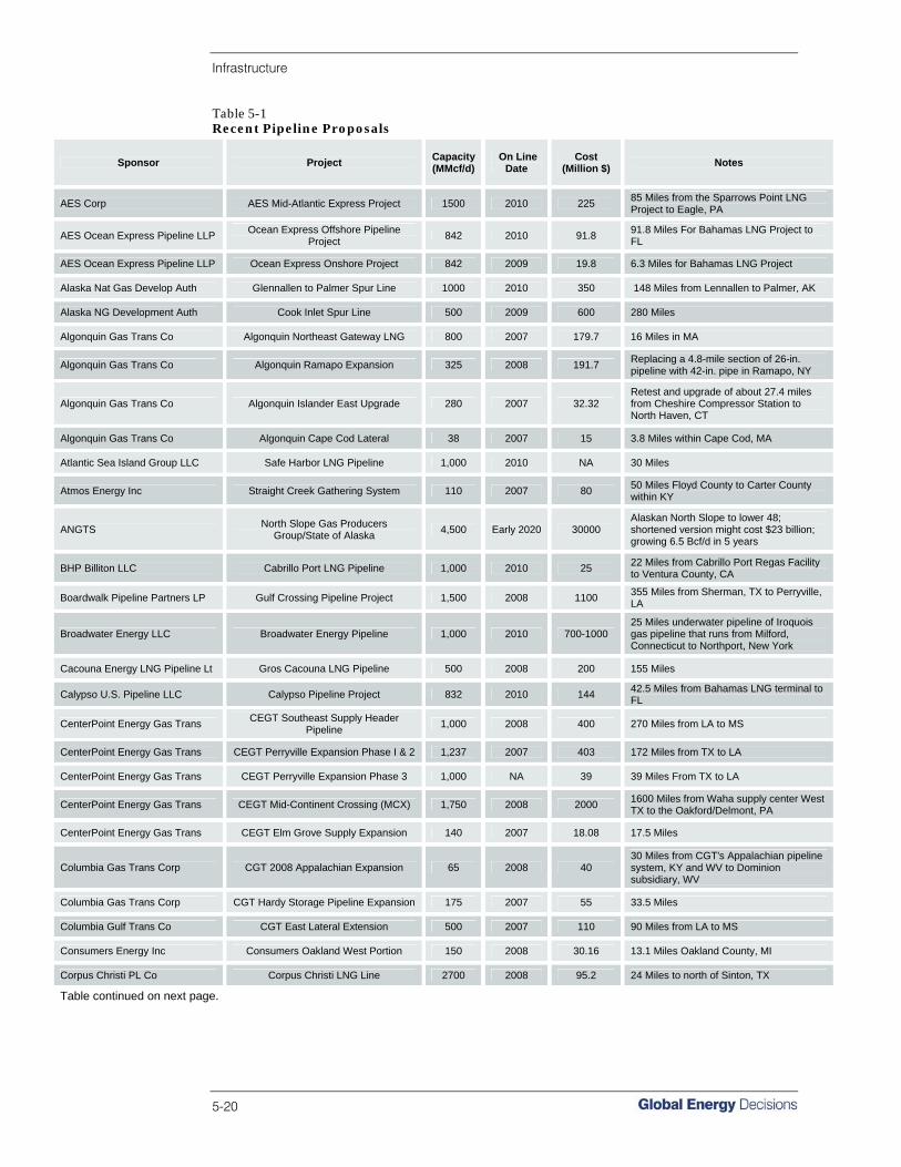
Infrastructure
5-20
Table 5-1 Recent Pipeline Proposals
Sponsor Project Capacity (MMcf/d)
On Line Date
Cost (Million $) Notes
AES Corp AES Mid-Atlantic Express Project 1500 2010 225 85 Miles from the Sparrows Point LNG Project to Eagle, PA
AES Ocean Express Pipeline LLP Ocean Express Offshore Pipeline Project 842 2010 91.8 91.8 Miles For Bahamas LNG Project to
FL
AES Ocean Express Pipeline LLP Ocean Express Onshore Project 842 2009 19.8 6.3 Miles for Bahamas LNG Project
Alaska Nat Gas Develop Auth Glennallen to Palmer Spur Line 1000 2010 350 148 Miles from Lennallen to Palmer, AK
Alaska NG Development Auth Cook Inlet Spur Line 500 2009 600 280 Miles
Algonquin Gas Trans Co Algonquin Northeast Gateway LNG 800 2007 179.7 16 Miles in MA
Algonquin Gas Trans Co Algonquin Ramapo Expansion 325 2008 191.7 Replacing a 4.8-mile section of 26-in. pipeline with 42-in. pipe in Ramapo, NY
Algonquin Gas Trans Co Algonquin Islander East Upgrade 280 2007 32.32 Retest and upgrade of about 27.4 miles from Cheshire Compressor Station to North Haven, CT
Algonquin Gas Trans Co Algonquin Cape Cod Lateral 38 2007 15 3.8 Miles within Cape Cod, MA
Atlantic Sea Island Group LLC Safe Harbor LNG Pipeline 1,000 2010 NA 30 Miles
Atmos Energy Inc Straight Creek Gathering System 110 2007 80 50 Miles Floyd County to Carter County within KY
ANGTS North Slope Gas Producers Group/State of Alaska 4,500 Early 2020 30000
Alaskan North Slope to lower 48; shortened version might cost $23 billion; growing 6.5 Bcf/d in 5 years
BHP Billiton LLC Cabrillo Port LNG Pipeline 1,000 2010 25 22 Miles from Cabrillo Port Regas Facility to Ventura County, CA
Boardwalk Pipeline Partners LP Gulf Crossing Pipeline Project 1,500 2008 1100 355 Miles from Sherman, TX to Perryville, LA
Broadwater Energy LLC Broadwater Energy Pipeline 1,000 2010 700-1000 25 Miles underwater pipeline of Iroquois gas pipeline that runs from Milford, Connecticut to Northport, New York
Cacouna Energy LNG Pipeline Lt Gros Cacouna LNG Pipeline 500 2008 200 155 Miles
Calypso U.S. Pipeline LLC Calypso Pipeline Project 832 2010 144 42.5 Miles from Bahamas LNG terminal to FL
CenterPoint Energy Gas Trans CEGT Southeast Supply Header Pipeline 1,000 2008 400 270 Miles from LA to MS
CenterPoint Energy Gas Trans CEGT Perryville Expansion Phase I & 2 1,237 2007 403 172 Miles from TX to LA
CenterPoint Energy Gas Trans CEGT Perryville Expansion Phase 3 1,000 NA 39 39 Miles From TX to LA
CenterPoint Energy Gas Trans CEGT Mid-Continent Crossing (MCX) 1,750 2008 2000 1600 Miles from Waha supply center West TX to the Oakford/Delmont, PA
CenterPoint Energy Gas Trans CEGT Elm Grove Supply Expansion 140 2007 18.08 17.5 Miles
Columbia Gas Trans Corp CGT 2008 Appalachian Expansion 65 2008 40 30 Miles from CGT's Appalachian pipeline system, KY and WV to Dominion subsidiary, WV
Columbia Gas Trans Corp CGT Hardy Storage Pipeline Expansion 175 2007 55 33.5 Miles
Columbia Gulf Trans Co CGT East Lateral Extension 500 2007 110 90 Miles from LA to MS
Consumers Energy Inc Consumers Oakland West Portion 150 2008 30.16 13.1 Miles Oakland County, MI
Corpus Christi PL Co Corpus Christi LNG Line 2700 2008 95.2 24 Miles to north of Sinton, TX
Table continued on next page.

Infrastructure
Gas Reference Case, Fall 2007 5-21
Sponsor Project Capacity (MMcf/d)
On Line Date
Cost (Million $) Notes
Creole Trail LLP Creole Trail Segments 2 & 3 3,300 2008 630 116.8 Miles Associated with LNG Terminal to Rayne, LA
Creole Trail LLP Creole Trail Segment 1 2,600 2008 101.7 18.1 Miles from the Creole Trail LNG terminal to interconnect with the Cheniere Sabine Pass Pipeline system
Crosstex Energy Co CrossTex LIG Extension 700 2007 225 65 Miles in LA
Crosstex Energy Services Inc Crosstex Azle Gas Plant Header 50 2007 40 30 Miles from Azle to the North Texas Pipeline
Dominion Cove Point LNG PL Co Dom Cove Point PL 2008 Expansion 800 2008 95 47.8 Miles in MD from Dominion Cove Point to interstate pipeline connections in VA
Dominion Transmission Inc Dominion 2008 PA Expansion 700 2008 190 81 Miles in PA
Dominion Transmission Inc TL-263 Expansion Project 21.25 2007 14.69 6.43 in Boone and Wyoming Counties, WV
Downeast LNG LLC Downeast LNG Lateral 625 2009 60 22 Miles from Robbinston, ME, to the Maritimes and Northeast Pipeline
Duke/Alliance/NJR Lebanon Connector Pipeline 1,000 2008 NA 120-170 Miles from Joliet, IL to Lebanon, OH
East Tennessee Nat Gas Co ETenn Jewell Ridge Lateral 235 Summer 2006 53 32 Miles in southwest VA
East Tennessee Nat Gas Co ETenn Patriot Extension III 75 2007 20 10 Miles
Eastern Shore Nat Gas Co EShore 2006 Expansion 26.2 Q4 2006 17.37 35 mile mainline extension and looping in PA and DE through 2006 to 2008
Eastern Shore Nat Gas Co EShore Cove Point Extension 60 2009 93 63 Miles
Eastern Shore Nat Gas Co EShore 2006 Expansion 10.3 Nov. 2006 17.4 35 Mile extension and looping in PA and DE
Eastern Shore Nat Gas Co EShore 2007 Expansion 10.3 Nov. 2007 8 11 Mile extension and looping in PA and DE
Eastern Shore Nat Gas Co EShore 2008 Expansion 10.85 Nov. 2008 8.2 9 Mile extension and looping in PA and DE
El Encino Pipeline El Encino-US Border Pipeline 500 2008 NA 239 miles
El Paso Natural Gas Co Paso Norte Pipeline Project 380 2008 453 396 Miles from NM, across the U.S.-Mexico border to power plants in Chihuahua and Durango
Emera Inc Brunswick Pipeline Lateral 850 2008 350 90 Miles from Canaport, NB, to a Canada-US border.
Empire Pipeline Co Empire/Millennium Expansion 250 2008 144.2
78 Miles of new 24-inch-diameter pipeline and associated facilities in Ontario, Yates, Schuyler, Chemung, and Steuben Counties, New York
Enbridge Energy Pipeline Co Marquez Plant Line 250 2007 20 15 Miles
Enbridge Energy Pipeline Co East Texas System Extension 700 2007 610 290 in TX
Enbridge Energy Pipeline Co Enbridge TX-MS Pipeline 1,000 2009 400 330 Miles from TX to MS
Enbridge Offshore Pipelines LL Neptune Deepwater Project 200 2009 50 11 Miles connecting to Hubline pipeline
Energy Transfer Co ET Barnett-Texoma Expansion 700 2007 360 264 Miles within TX
Energy Transfer Co ET FW Basin to Texoma Pipeline 700 2007 300 135 Miles from the Partnership’s existing Fort Worth Basin system to its 30” Texoma pipeline in Lamar County, TX
Enterprise Products Partners Enterprise Sherman Extension 1,100 Q4 2008 400 178 Miles in Morgan Mill-Barnett Shale-Sherman
Equitrans LP Big Sandy Pipeline Phase I 70 2007 80 67.61 Miles in eastern Kentucky
Table continued on next page.
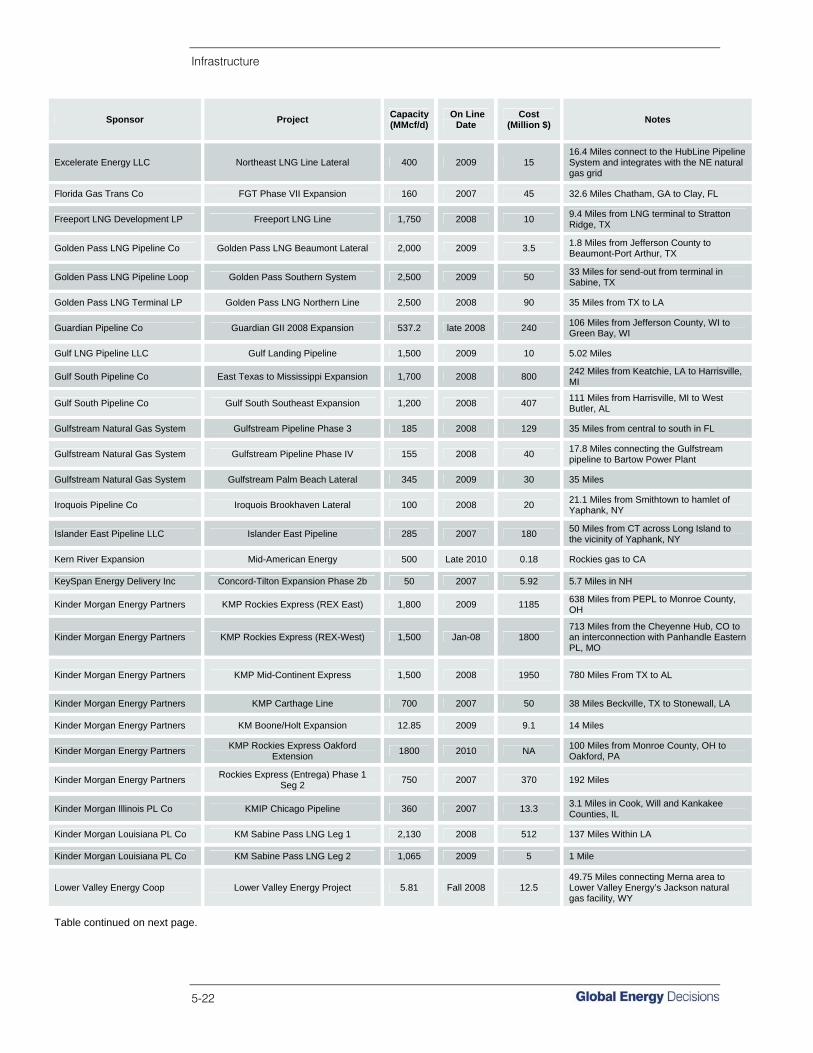
Infrastructure
5-22
Sponsor Project Capacity (MMcf/d)
On Line Date
Cost (Million $) Notes
Excelerate Energy LLC Northeast LNG Line Lateral 400 2009 15 16.4 Miles connect to the HubLine Pipeline System and integrates with the NE natural gas grid
Florida Gas Trans Co FGT Phase VII Expansion 160 2007 45 32.6 Miles Chatham, GA to Clay, FL
Freeport LNG Development LP Freeport LNG Line 1,750 2008 10 9.4 Miles from LNG terminal to Stratton Ridge, TX
Golden Pass LNG Pipeline Co Golden Pass LNG Beaumont Lateral 2,000 2009 3.5 1.8 Miles from Jefferson County to Beaumont-Port Arthur, TX
Golden Pass LNG Pipeline Loop Golden Pass Southern System 2,500 2009 50 33 Miles for send-out from terminal in Sabine, TX
Golden Pass LNG Terminal LP Golden Pass LNG Northern Line 2,500 2008 90 35 Miles from TX to LA
Guardian Pipeline Co Guardian GII 2008 Expansion 537.2 late 2008 240 106 Miles from Jefferson County, WI to Green Bay, WI
Gulf LNG Pipeline LLC Gulf Landing Pipeline 1,500 2009 10 5.02 Miles
Gulf South Pipeline Co East Texas to Mississippi Expansion 1,700 2008 800 242 Miles from Keatchie, LA to Harrisville, MI
Gulf South Pipeline Co Gulf South Southeast Expansion 1,200 2008 407 111 Miles from Harrisville, MI to West Butler, AL
Gulfstream Natural Gas System Gulfstream Pipeline Phase 3 185 2008 129 35 Miles from central to south in FL
Gulfstream Natural Gas System Gulfstream Pipeline Phase IV 155 2008 40 17.8 Miles connecting the Gulfstream pipeline to Bartow Power Plant
Gulfstream Natural Gas System Gulfstream Palm Beach Lateral 345 2009 30 35 Miles
Iroquois Pipeline Co Iroquois Brookhaven Lateral 100 2008 20 21.1 Miles from Smithtown to hamlet of Yaphank, NY
Islander East Pipeline LLC Islander East Pipeline 285 2007 180 50 Miles from CT across Long Island to the vicinity of Yaphank, NY
Kern River Expansion Mid-American Energy 500 Late 2010 0.18 Rockies gas to CA
KeySpan Energy Delivery Inc Concord-Tilton Expansion Phase 2b 50 2007 5.92 5.7 Miles in NH
Kinder Morgan Energy Partners KMP Rockies Express (REX East) 1,800 2009 1185 638 Miles from PEPL to Monroe County, OH
Kinder Morgan Energy Partners KMP Rockies Express (REX-West) 1,500 Jan-08 1800 713 Miles from the Cheyenne Hub, CO to an interconnection with Panhandle Eastern PL, MO
Kinder Morgan Energy Partners KMP Mid-Continent Express 1,500 2008
1950
780 Miles From TX to AL
Kinder Morgan Energy Partners KMP Carthage Line 700 2007 50 38 Miles Beckville, TX to Stonewall, LA
Kinder Morgan Energy Partners KM Boone/Holt Expansion 12.85 2009 9.1 14 Miles
Kinder Morgan Energy Partners KMP Rockies Express Oakford Extension 1800 2010 NA 100 Miles from Monroe County, OH to
Oakford, PA
Kinder Morgan Energy Partners Rockies Express (Entrega) Phase 1 Seg 2 750 2007 370 192 Miles
Kinder Morgan Illinois PL Co KMIP Chicago Pipeline 360 2007 13.3 3.1 Miles in Cook, Will and Kankakee Counties, IL
Kinder Morgan Louisiana PL Co KM Sabine Pass LNG Leg 1 2,130 2008 512 137 Miles Within LA
Kinder Morgan Louisiana PL Co KM Sabine Pass LNG Leg 2 1,065 2009 5 1 Mile
Lower Valley Energy Coop Lower Valley Energy Project 5.81 Fall 2008 12.5 49.75 Miles connecting Merna area to Lower Valley Energy’s Jackson natural gas facility, WY
Table continued on next page.
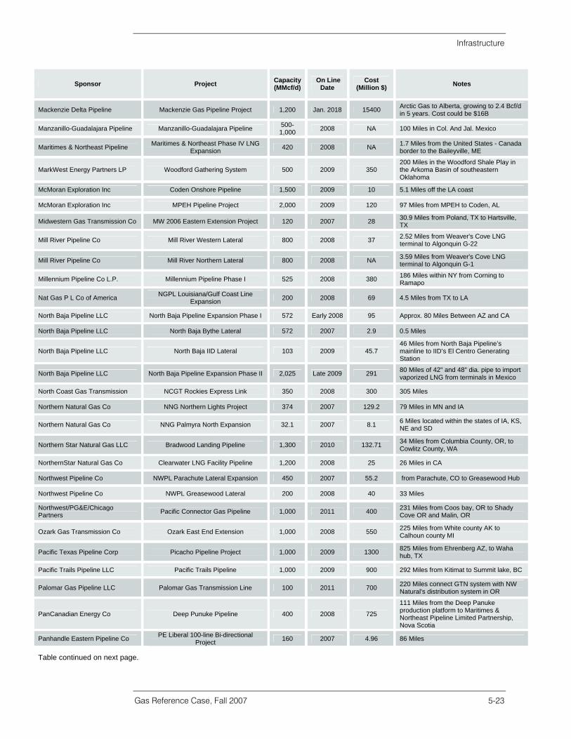
Infrastructure
Gas Reference Case, Fall 2007 5-23
Sponsor Project Capacity (MMcf/d)
On Line Date
Cost (Million $) Notes
Mackenzie Delta Pipeline Mackenzie Gas Pipeline Project 1,200 Jan. 2018 15400 Arctic Gas to Alberta, growing to 2.4 Bcf/d in 5 years. Cost could be $16B
Manzanillo-Guadalajara Pipeline Manzanillo-Guadalajara Pipeline 500-1,000 2008 NA 100 Miles in Col. And Jal. Mexico
Maritimes & Northeast Pipeline Maritimes & Northeast Phase IV LNG Expansion 420 2008 NA 1.7 Miles from the United States - Canada
border to the Baileyville, ME
MarkWest Energy Partners LP Woodford Gathering System 500 2009 350 200 Miles in the Woodford Shale Play in the Arkoma Basin of southeastern Oklahoma
McMoran Exploration Inc Coden Onshore Pipeline 1,500 2009 10 5.1 Miles off the LA coast
McMoran Exploration Inc MPEH Pipeline Project 2,000 2009 120 97 Miles from MPEH to Coden, AL
Midwestern Gas Transmission Co MW 2006 Eastern Extension Project 120 2007 28 30.9 Miles from Poland, TX to Hartsville, TX
Mill River Pipeline Co Mill River Western Lateral 800 2008 37 2.52 Miles from Weaver's Cove LNG terminal to Algonquin G-22
Mill River Pipeline Co Mill River Northern Lateral 800 2008 NA 3.59 Miles from Weaver's Cove LNG terminal to Algonquin G-1
Millennium Pipeline Co L.P. Millennium Pipeline Phase I 525 2008 380 186 Miles within NY from Corning to Ramapo
Nat Gas P L Co of America NGPL Louisiana/Gulf Coast Line Expansion 200 2008 69 4.5 Miles from TX to LA
North Baja Pipeline LLC North Baja Pipeline Expansion Phase I 572 Early 2008 95 Approx. 80 Miles Between AZ and CA
North Baja Pipeline LLC North Baja Bythe Lateral 572 2007 2.9 0.5 Miles
North Baja Pipeline LLC North Baja IID Lateral 103 2009 45.7 46 Miles from North Baja Pipeline’s mainline to IID’s El Centro Generating Station
North Baja Pipeline LLC North Baja Pipeline Expansion Phase II 2,025 Late 2009 291 80 Miles of 42" and 48" dia. pipe to import vaporized LNG from terminals in Mexico
North Coast Gas Transmission NCGT Rockies Express Link 350 2008 300 305 Miles
Northern Natural Gas Co NNG Northern Lights Project 374 2007 129.2 79 Miles in MN and IA
Northern Natural Gas Co NNG Palmyra North Expansion 32.1 2007 8.1 6 Miles located within the states of IA, KS, NE and SD
Northern Star Natural Gas LLC Bradwood Landing Pipeline 1,300 2010 132.71 34 Miles from Columbia County, OR, to Cowlitz County, WA
NorthernStar Natural Gas Co Clearwater LNG Facility Pipeline 1,200 2008 25 26 Miles in CA
Northwest Pipeline Co NWPL Parachute Lateral Expansion 450 2007 55.2 from Parachute, CO to Greasewood Hub
Northwest Pipeline Co NWPL Greasewood Lateral 200 2008 40 33 Miles
Northwest/PG&E/Chicago Partners Pacific Connector Gas Pipeline 1,000 2011 400 231 Miles from Coos bay, OR to Shady
Cove OR and Malin, OR
Ozark Gas Transmission Co Ozark East End Extension 1,000 2008 550 225 Miles from White county AK to Calhoun county MI
Pacific Texas Pipeline Corp Picacho Pipeline Project 1,000 2009 1300 825 Miles from Ehrenberg AZ, to Waha hub, TX
Pacific Trails Pipeline LLC Pacific Trails Pipeline 1,000 2009 900 292 Miles from Kitimat to Summit lake, BC
Palomar Gas Pipeline LLC Palomar Gas Transmission Line 100 2011 700 220 Miles connect GTN system with NW Natural's distribution system in OR
PanCanadian Energy Co Deep Punuke Pipeline 400 2008 725
111 Miles from the Deep Panuke production platform to Maritimes & Northeast Pipeline Limited Partnership, Nova Scotia
Panhandle Eastern Pipeline Co PE Liberal 100-line Bi-directional Project 160 2007 4.96 86 Miles
Table continued on next page.

Infrastructure
5-24
Sponsor Project Capacity (MMcf/d)
On Line Date
Cost (Million $) Notes
Pine Prairie Corridors Pine Prairie Miller’s Lake Lateral 600 2007 28 14 Miles
Point Comfort Pipeline Co Point Comfort LNG Line 1,000 2010 62.58 27.07Miles from Colhoun LNG
Port Arthur Pipeline LLP Port Arthur LNG Laterals Phase II 1,300 2010 10.4 3 Miles from terminal in Port Arthur, Jefferson County, TX
Port Arthur Pipeline LLP Port Arthur LNG Laterals Phase I 1,700 2008 206.5 70 Miles from TX to LA
Port Barre Investments LLC Bobcat Storage Lateral 1,200 2008 20 16.1 Miles Meter Station to the Gas Storage Site
Questar Overthrust Pipeline Co Overthrust Wamsutter Extension 750 2008 NA 77 Miles from Kanda to Wamsutter, WY
Questar Pipeline Co Questar Southern System 2008 Expansion 540 2008 NA 300 Miles
Questar Pipeline Co Questar Southern System Expansion to Goshen 170 2007 60 58 Miles
Quoddy Bay LLC Quoddy Bay LNG Lateral 2,000 2009 NA 35.8 Miles from LNG terminal in Perry to interstate pipeline Princeton, ME
Rendezvous Gas Services LLC Rendezvous Black Fork Lateral 450 2007 60 98 Miles
Sabine Pass PL Co Sabine Pass LNG Line 2,600 2008 350 16 Miles from terminal to Johnson's Bayou
San Patricio Pipeline LLC Ingleside LNG Line 1,000 2008 53.5 26.4 Miles from Ingleside's LNG terminal to interconnections with several interstate and intrastate pipelines
Sempra Energy Inc Cameron Interstate Pipeline 1,500 2008 29.8 36.1 Miles in LA
SG Interests (SG) Co Bull Mountain Pipeline Project 100 2007 30 25.5 through portions of Gunnison, Delta, Mesa, and Garfield Counties, CO
SGR Holding Corporation Southern Pines Storage Line Extention 600 2007 32 26 Miles
Sonora Pipeline Co Sonoran LNG Distribution System 1,300 2008 NA 350 Miles
Sonora Pipeline LLC Sonora Burgos Hub Mission Line 500 2008 0.5 25 Miles
Sonora Pipeline LLC Sonora Burgos Hub Progresso Line 500 2008 NA 10 Miles
Sound Energy Solutions Inc Long Beach LNG Sendout Pipeline 700 2008 4 2.3 Miles from LNG terminal to SoCal's line 765 at Salt work station, CA
Southern Natural Gas Co SONAT Cypress 2010 Phase 2&3 116 2010 81 10 Miles within GA
Southern Natural Gas Co SONAT Cypress 2007 Phase 1 220 2007 240 16.7 Miles From Elba Island LNG, GA to FL
Southern Natural Gas Co SONAT Elba Express 1,200 2010 200 190 Miles within GA
Southern Natural Gas Co New Home Storage Lateral Phase 1 700 2011 12 9 Miles connecting SNG's existing underground pipeline system
Southern Natural Gas Co New Home Storage Lateral Phase 2 700 2014 12 9 Miles connecting SNG's existing underground pipeline system
Southern Natural Gas Co SONAT Express Northern Segment 945 2012 NA 83.8 Miles
Stark Gas Storage LLC Stark Storage Pipeline 800 2007 55 35 Miles
Tampa Electric Co Gulfstream Bayside Lateral 48 2007 NA 28 Miles Within FL
Tennessee Gas Pipeline Co Tenneco Deepwater Link Project 1,000 2007 10.2 1 Mile
Tennessee Gas Pipeline Co Tenneco Essex-Middlesex Expansion 82.3 2007 38 7.87 Miles
Tennessee Gas Pipeline Co Tenneco Triple-T Extension 200 2007 22 6.23 Miles
TEPPCO TEPPCO Bird Canyon Lateral 100 2007 NA 31 Miles
TEPPCO TEPPCO Bridger Corridor Lateral 100 2007 NA 44 Miles
Table continued on next page.
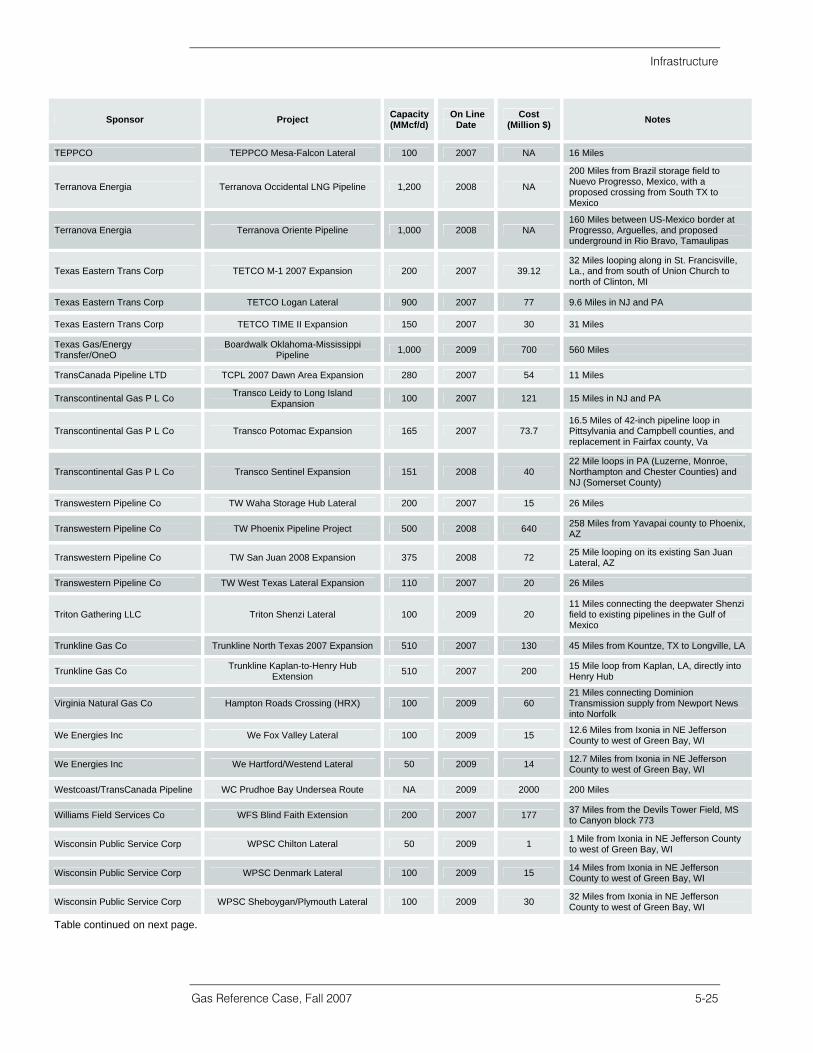
Infrastructure
Gas Reference Case, Fall 2007 5-25
Sponsor Project Capacity (MMcf/d)
On Line Date
Cost (Million $) Notes
TEPPCO TEPPCO Mesa-Falcon Lateral 100 2007 NA 16 Miles
Terranova Energia Terranova Occidental LNG Pipeline 1,200 2008 NA
200 Miles from Brazil storage field to Nuevo Progresso, Mexico, with a proposed crossing from South TX to Mexico
Terranova Energia Terranova Oriente Pipeline 1,000 2008 NA 160 Miles between US-Mexico border at Progresso, Arguelles, and proposed underground in Rio Bravo, Tamaulipas
Texas Eastern Trans Corp TETCO M-1 2007 Expansion 200 2007 39.12 32 Miles looping along in St. Francisville, La., and from south of Union Church to north of Clinton, MI
Texas Eastern Trans Corp TETCO Logan Lateral 900 2007 77 9.6 Miles in NJ and PA
Texas Eastern Trans Corp TETCO TIME II Expansion 150 2007 30 31 Miles
Texas Gas/Energy Transfer/OneO
Boardwalk Oklahoma-Mississippi Pipeline 1,000 2009 700 560 Miles
TransCanada Pipeline LTD TCPL 2007 Dawn Area Expansion 280 2007 54 11 Miles
Transcontinental Gas P L Co Transco Leidy to Long Island Expansion 100 2007 121 15 Miles in NJ and PA
Transcontinental Gas P L Co Transco Potomac Expansion 165 2007 73.7 16.5 Miles of 42-inch pipeline loop in Pittsylvania and Campbell counties, and replacement in Fairfax county, Va
Transcontinental Gas P L Co Transco Sentinel Expansion 151 2008 40 22 Mile loops in PA (Luzerne, Monroe, Northampton and Chester Counties) and NJ (Somerset County)
Transwestern Pipeline Co TW Waha Storage Hub Lateral 200 2007 15 26 Miles
Transwestern Pipeline Co TW Phoenix Pipeline Project 500 2008 640 258 Miles from Yavapai county to Phoenix, AZ
Transwestern Pipeline Co TW San Juan 2008 Expansion 375 2008 72 25 Mile looping on its existing San Juan Lateral, AZ
Transwestern Pipeline Co TW West Texas Lateral Expansion 110 2007 20 26 Miles
Triton Gathering LLC Triton Shenzi Lateral 100 2009 20 11 Miles connecting the deepwater Shenzi field to existing pipelines in the Gulf of Mexico
Trunkline Gas Co Trunkline North Texas 2007 Expansion 510 2007 130 45 Miles from Kountze, TX to Longville, LA
Trunkline Gas Co Trunkline Kaplan-to-Henry Hub Extension 510 2007 200 15 Mile loop from Kaplan, LA, directly into
Henry Hub
Virginia Natural Gas Co Hampton Roads Crossing (HRX) 100 2009 60 21 Miles connecting Dominion Transmission supply from Newport News into Norfolk
We Energies Inc We Fox Valley Lateral 100 2009 15 12.6 Miles from Ixonia in NE Jefferson County to west of Green Bay, WI
We Energies Inc We Hartford/Westend Lateral 50 2009 14 12.7 Miles from Ixonia in NE Jefferson County to west of Green Bay, WI
Westcoast/TransCanada Pipeline WC Prudhoe Bay Undersea Route NA 2009 2000 200 Miles
Williams Field Services Co WFS Blind Faith Extension 200 2007 177 37 Miles from the Devils Tower Field, MS to Canyon block 773
Wisconsin Public Service Corp WPSC Chilton Lateral 50 2009 1 1 Mile from Ixonia in NE Jefferson County to west of Green Bay, WI
Wisconsin Public Service Corp WPSC Denmark Lateral 100 2009 15 14 Miles from Ixonia in NE Jefferson County to west of Green Bay, WI
Wisconsin Public Service Corp WPSC Sheboygan/Plymouth Lateral 100 2009 30 32 Miles from Ixonia in NE Jefferson County to west of Green Bay, WI
Table continued on next page.
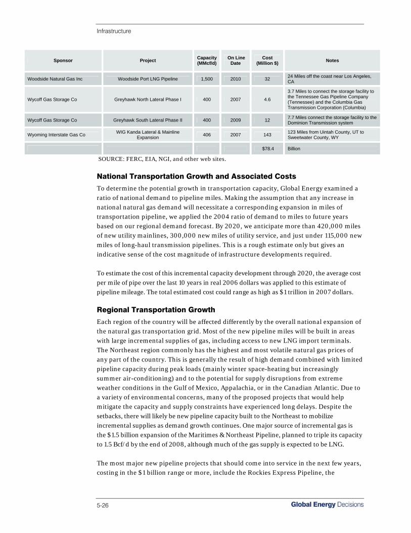
Infrastructure
5-26
Sponsor Project Capacity (MMcf/d)
On Line Date
Cost (Million $) Notes
Woodside Natural Gas Inc Woodside Port LNG Pipeline 1,500 2010 32 24 Miles off the coast near Los Angeles, CA
Wycoff Gas Storage Co Greyhawk North Lateral Phase I 400 2007 4.6
3.7 Miles to connect the storage facility to the Tennessee Gas Pipeline Company (Tennessee) and the Columbia Gas Transmission Corporation (Columbia)
Wycoff Gas Storage Co Greyhawk South Lateral Phase II 400 2009 12 7.7 Miles connect the storage facility to the Dominion Transmission system
Wyoming Interstate Gas Co WIG Kanda Lateral & Mainline Expansion 406 2007 143 123 Miles from Uintah County, UT to
Sweetwater County, WY
$78.4 Billion
SOURCE: FERC, EIA, NGI, and other web sites.
National Transportation Growth and Associated Costs
To determine the potential growth in transportation capacity, Global Energy examined a ratio of national demand to pipeline miles. Making the assumption that any increase in national natural gas demand will necessitate a corresponding expansion in miles of transportation pipeline, we applied the 2004 ratio of demand to miles to future years based on our regional demand forecast. By 2020, we anticipate more than 420,000 miles of new utility mainlines, 300,000 new miles of utility service, and just under 115,000 new miles of long-haul transmission pipelines. This is a rough estimate only but gives an indicative sense of the cost magnitude of infrastructure developments required. To estimate the cost of this incremental capacity development through 2020, the average cost per mile of pipe over the last 10 years in real 2006 dollars was applied to this estimate of pipeline mileage. The total estimated cost could range as high as $1 trillion in 2007 dollars. Regional Transportation Growth
Each region of the country will be affected differently by the overall national expansion of the natural gas transportation grid. Most of the new pipeline miles will be built in areas with large incremental supplies of gas, including access to new LNG import terminals. The Northeast region commonly has the highest and most volatile natural gas prices of any part of the country. This is generally the result of high demand combined with limited pipeline capacity during peak loads (mainly winter space-heating but increasingly summer air-conditioning) and to the potential for supply disruptions from extreme weather conditions in the Gulf of Mexico, Appalachia, or in the Canadian Atlantic. Due to a variety of environmental concerns, many of the proposed projects that would help mitigate the capacity and supply constraints have experienced long delays. Despite the setbacks, there will likely be new pipeline capacity built to the Northeast to mobilize incremental supplies as demand growth continues. One major source of incremental gas is the $1.5 billion expansion of the Maritimes & Northeast Pipeline, planned to triple its capacity to 1.5 Bcf/d by the end of 2008, although much of the gas supply is expected to be LNG. The most major new pipeline projects that should come into service in the next few years, costing in the $1 billion range or more, include the Rockies Express Pipeline, the

Infrastructure
Gas Reference Case, Fall 2007 5-27
Millennium/Empire Pipeline, Mid-Continent Express project, and the Maritimes & Northeast Pipeline (M&NE) Expansion project. Kinder Morgan Energy’s Rockies Express (in the $3.0 to $4.0 billion range total) would transport 1.8 Bcf/d of land-locked Rocky Mountain gas from Colorado to the Ohio/Pennsylvania border (including the Leidy storage fields), a distance of about 1,200 miles. Millennium/Empire (about $0.8 billion total) is sponsored by NiSource, KeySpan, and DTE Energy and would provide at least 0.525 Bcf/d service from upper-New York State and deliver gas to New York City. FERC issued a construction certificate in December 2006 for the 264-mile project. Kinder Morgan’s Mid-Continent Express project (about $1.75 billion) would deliver 1.5 Bcf/d of unconventional gas from key production areas—such as the Barnett Shale in North Texas, Arkoma Basin in Oklahoma, and the Fayetteville Shale in Arkansas—to Alabama and of course further downstream. All three of these pipelines have experienced significant delays over the years, including environmental ones. Stranded gas in the Rocky Mountain region during the last year occasionally dropped to the $1.50 to $3.00/MMBtu range while Henry Hub prices hovered in the $6.00 to $8.00/MMBtu range, indicating that it would be well worthwhile to relieve this congestion with additional pipeline from this region westward to California as well as eastward to the New York/New Jersey/New England region, which has the highest basis differentials in the country. Finally, the $1.5 billion Maritimes & Northeast Expansion would transport about 1.5 Bcf/d re-gasified LNG from Canadian terminals in New Brunswick down to Dracut, Massachusetts, and the greater Boston area via an expansion within their already existing right-of-way. This would involve additional pipeline construction, additional compressor stations, and re-rating the pipeline’s MAOP (maximum allowable operating pressure) from 1,440 psig to 1,600 psig. Natural Gas Storage Infrastructure in the United States
According to the EIA, at the end of 2006 the United States had 8,268 Bcf of total natural gas storage, of which about 3,730 Bcf was working gas. During the next 25 years, the expansion of storage capacity will have to keep pace with America’s appetite for natural gas, not only to serve customers’ needs but to prevent excess volatility during times of high demand. For example, for nearly a four-week period starting on January 25, 2007 the New York/New Jersey/New England citygate price of gas was over $10/dth, and sometimes in excess of $30/dth. For a time, even citygate prices in Florida were in excess of $10/dth. Supply delivery problems have become more frequent, natural gas prices have reached new highs, and price volatility is rampant. This has resulted in a flurry of activity in the LNG market, but it is unlikely that sufficient LNG import terminals will be built where needed to address these pricing issues. Moreover, any LNG terminals that are built will place a strain on existing pipelines. Underground natural gas storage projects can address many of these issues, depending on where they are located and the types of field being developed. To help relieve this strain, the EPAct of 2005 formally changed FERC policy to allow market-based rates, rather than solely cost-based rates, to encourage capital investment in storage facilities. In early 2007, FERC Chairman Joseph T. Kelliher observed:
“There is a great deal of concern about natural gas price volatility. One of the best ways to guard against volatility is by increasing gas storage capacity. The Commission is acting to

Infrastructure
5-28
encourage expansion of gas storage capacity, and has adopted pricing reforms to that end.”
This expansion of differing types of storage, as with gas transportation, will require significant investment in existing facilities and development of new capacity in production areas and at LNG regasification terminals, especially in market areas. There are three major types of reservoirs used for natural gas storage: 1. Depleted oil/gas reservoirs; 2. Aquifers; and 3. Salt storage (domal and bedded).
Each storage reservoir has very specific operating and cycling parameters that depend on the reservoir geology of the structure and on installed compression capacity. Salt reservoirs have the highest deliverability and multi-cycling capacity, but the majority of working natural gas storage resides in depleted oil and gas reservoirs. An increase in the demand for natural gas, especially LNG, will also increase the need for more gas storage capacity. Storage is needed to meet peak-day demand, to ensure reliable supply, and to capture the optionality value of seasonal and daily price volatility. Although some supply area storage was developed, most storage capacity was developed in market areas. Figure 5-16 U.S. Underground Storage Capacity by Type of Reservoir
0
1,000
2,000
3,000
4,000
5,000
6,000
7,000
8,000
9,000
10,000
1999 2000 2001 2002 2003 2004 2005 2006
Bcf
0
45
90
135
180
225
270
315
360
405
450
Salt Caverns
Acquifers
Depleted Fields
Number of Storage Fields
SOURCE: EIA and Global Energy.

Infrastructure
Gas Reference Case, Fall 2007 5-29
Storage development should continue to expand in market areas with dynamic weather-driven swings in peak load, and with the expansion of Atlantic Coast LNG import terminals (Canadian and U.S.). At the terminals, regasified LNG can be stored to unload the 7-12 days of cryogenic storage to meet shipping schedules. Production area, high deliverability (multi-cycling) storage in salt reservoirs should also grow to meet competition from LNG’s cryogenic storage and its instant swing capacity. There will also be increased use of low deliverability (single cycle) storage in depleted reservoirs to meet the “re-storage” of regasified LNG needed for LNG to capture seasonal loads. Although salt caverns represented only 3 percent of national storage capacity in 2005, this type of capacity is increasing because salt caverns allow for much greater flexibility in both injections and withdrawals. In a 2003 report on storage expansions, the EIA reported that “[p]roposed salt cavern (31) storage projects represent 46 percent of all additional working gas capacity (158 Bcf) and 69 percent (11.5 Bcf/d) of additional deliverability which could be installed over the next five years.2 The rapid cycling capability of salt cavern storage, coupled with its ability to respond quickly to daily, even hourly, variations in customer needs, has made it very attractive for storage developers, whose profitability is often dependent upon their capability to maximize turnover volumes.” Salt cavern storage can respond to daily and even hourly swing loads. The economic performance benefits because lower unit costs and profitability are generally tied to the level of volume cycling and its associated compression capacity. By applying a ratio of storage capacity necessary to meet natural gas demand in 2004 to future years, one can estimate the probable increase in national storage capacity. By 2020, we expect to see U.S. working gas storage capacity reach 5,224 Bcf. At a cost of $6 million 2005 dollars per Bcf of incremental working gas capacity for low deliverability storage and $18 million per Bcf for high deliverability storage, a cost between $9 billion (for 100 percent low deliverability) and $27 billion (for 100 percent high deliverability) would be incurred for new storage capacity to meet projected incremental demand. The following figure outlines regional storage activity variations and the very gradual rise in working storage inventories over the last decade.
2 EIA, 2003, U.S. Natural Gas Pipeline and Underground Storage Expansions in 2003.
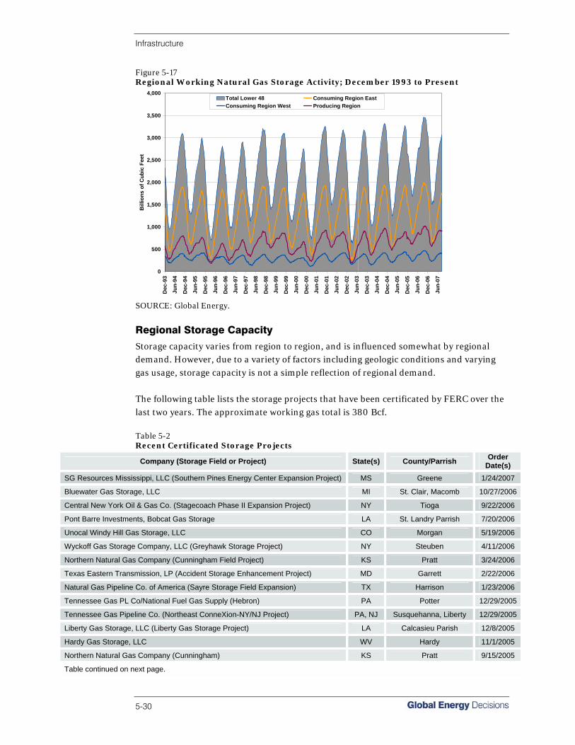
Infrastructure
5-30
Figure 5-17 Regional Working Natural Gas Storage Activity; December 1993 to Present
Regional Working Natural Gas Storage Inventory
0
500
1,000
1,500
2,000
2,500
3,000
3,500
4,000
Dec
-93
Jun-
94
Dec
-94
Jun-
95
Dec
-95
Jun-
96
Dec
-96
Jun-
97
Dec
-97
Jun-
98
Dec
-98
Jun-
99
Dec
-99
Jun-
00
Dec
-00
Jun-
01
Dec
-01
Jun-
02
Dec
-02
Jun-
03
Dec
-03
Jun-
04
Dec
-04
Jun-
05
Dec
-05
Jun-
06
Dec
-06
Jun-
07
Bill
ions
of C
ubic
Fee
t
Total Lower 48 Consuming Region EastConsuming Region West Producing Region
SOURCE: Global Energy.
Regional Storage Capacity
Storage capacity varies from region to region, and is influenced somewhat by regional demand. However, due to a variety of factors including geologic conditions and varying gas usage, storage capacity is not a simple reflection of regional demand. The following table lists the storage projects that have been certificated by FERC over the last two years. The approximate working gas total is 380 Bcf. Table 5-2 Recent Certificated Storage Projects
Company (Storage Field or Project) State(s) County/Parrish Order Date(s)
SG Resources Mississippi, LLC (Southern Pines Energy Center Expansion Project) MS Greene 1/24/2007
Bluewater Gas Storage, LLC MI St. Clair, Macomb 10/27/2006
Central New York Oil & Gas Co. (Stagecoach Phase II Expansion Project) NY Tioga 9/22/2006
Pont Barre Investments, Bobcat Gas Storage LA St. Landry Parrish 7/20/2006
Unocal Windy Hill Gas Storage, LLC CO Morgan 5/19/2006
Wyckoff Gas Storage Company, LLC (Greyhawk Storage Project) NY Steuben 4/11/2006
Northern Natural Gas Company (Cunningham Field Project) KS Pratt 3/24/2006
Texas Eastern Transmission, LP (Accident Storage Enhancement Project) MD Garrett 2/22/2006
Natural Gas Pipeline Co. of America (Sayre Storage Field Expansion) TX Harrison 1/23/2006
Tennessee Gas PL Co/National Fuel Gas Supply (Hebron) PA Potter 12/29/2005
Tennessee Gas Pipeline Co. (Northeast ConneXion-NY/NJ Project) PA, NJ Susquehanna, Liberty 12/29/2005
Liberty Gas Storage, LLC (Liberty Gas Storage Project) LA Calcasieu Parish 12/8/2005
Hardy Gas Storage, LLC WV Hardy 11/1/2005
Northern Natural Gas Company (Cunningham) KS Pratt 9/15/2005
Table continued on next page.
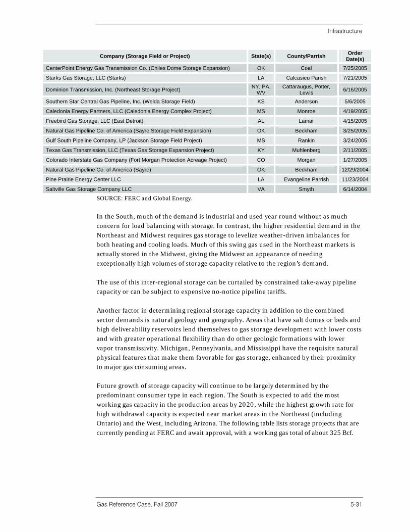
Infrastructure
Gas Reference Case, Fall 2007 5-31
Company (Storage Field or Project) State(s) County/Parrish Order Date(s)
CenterPoint Energy Gas Transmission Co. (Chiles Dome Storage Expansion) OK Coal 7/25/2005
Starks Gas Storage, LLC (Starks) LA Calcasieu Parish 7/21/2005
Dominion Transmission, Inc. (Northeast Storage Project) NY, PA, WV
Cattaraugus, Potter, Lewis 6/16/2005
Southern Star Central Gas Pipeline, Inc. (Welda Storage Field) KS Anderson 5/6/2005
Caledonia Energy Partners, LLC (Caledonia Energy Complex Project) MS Monroe 4/19/2005
Freebird Gas Storage, LLC (East Detroit) AL Lamar 4/15/2005
Natural Gas Pipeline Co. of America (Sayre Storage Field Expansion) OK Beckham 3/25/2005
Gulf South Pipeline Company, LP (Jackson Storage Field Project) MS Rankin 3/24/2005
Texas Gas Transmission, LLC (Texas Gas Storage Expansion Project) KY Muhlenberg 2/11/2005
Colorado Interstate Gas Company (Fort Morgan Protection Acreage Project) CO Morgan 1/27/2005
Natural Gas Pipeline Co. of America (Sayre) OK Beckham 12/29/2004
Pine Prairie Energy Center LLC LA Evangeline Parrish 11/23/2004
Saltville Gas Storage Company LLC VA Smyth 6/14/2004
SOURCE: FERC and Global Energy. In the South, much of the demand is industrial and used year round without as much concern for load balancing with storage. In contrast, the higher residential demand in the Northeast and Midwest requires gas storage to levelize weather-driven imbalances for both heating and cooling loads. Much of this swing gas used in the Northeast markets is actually stored in the Midwest, giving the Midwest an appearance of needing exceptionally high volumes of storage capacity relative to the region’s demand. The use of this inter-regional storage can be curtailed by constrained take-away pipeline capacity or can be subject to expensive no-notice pipeline tariffs. Another factor in determining regional storage capacity in addition to the combined sector demands is natural geology and geography. Areas that have salt domes or beds and high deliverability reservoirs lend themselves to gas storage development with lower costs and with greater operational flexibility than do other geologic formations with lower vapor transmissivity. Michigan, Pennsylvania, and Mississippi have the requisite natural physical features that make them favorable for gas storage, enhanced by their proximity to major gas consuming areas. Future growth of storage capacity will continue to be largely determined by the predominant consumer type in each region. The South is expected to add the most working gas capacity in the production areas by 2020, while the highest growth rate for high withdrawal capacity is expected near market areas in the Northeast (including Ontario) and the West, including Arizona. The following table lists storage projects that are currently pending at FERC and await approval, with a working gas total of about 325 Bcf.

Infrastructure
5-32
Table 5-3 Pending Storage Projects
Company (Storage Field or Project) State County/ Parish Docket Working
Gas Capacity
(Bcf)
MoBay Gas Storage Hub AL Mobile Bay CP06-398 50
Northern Natural Gas Company Redfield Expansion IA Dallas CP07-108 8.55
Mississippi Hub, LLC MS Simpson CP07-4 12 ANR Pipeline Company Storage Enhancement Project - 2008 MI Kalkaska CP06-464 14.7
Golden Triangle Storage, Inc. TX Jefferson, Orange CP07-414 12 Southern Star Central Gas Pipeline, Inc. (Piqua Storage Field Expansion) KS Allen CP07-17 3.2
Puget Sound Energy, Inc. (Operator/JP Storage Project) WA Lewis CP06-412 10.5
Northwest Pipeline Corporation (Jackson Prairie Deliverability Expansion) WA Lewis CP06-416 10.5
Petal Gas Storage, LLC (Petal Caverns Conversion Project) MS Forrest CP07-30 4.5
Dominion Transmission, Inc. (USA Storage Project) PA Potter CP07-31 4.4
Eagan Hub Storage, LLC LA Acadia CP07-88 8
Texas Gas Transmission, LLC KY Muhlenburg CP07-405 8.25
Copiah Storage, LLC MS Copiah CP02-25 12.2
Columbia Gas Transmission, Eastern Market Expansion OH, VA, WV Multiple Counties CP07-367 5.7
Tres Palacios Gas Storage, LLC TX Matagorda, Wharton CP07-90 36
Enstor Houston Hub Storage and Transportation TX Liberty CP07-390 30
Monroe Gas Storage Company, LLC MS Monroe CP07-406 12
Arizona Natural Gas Storage Project (El Paso) AZ N/A N/A 3.5
Black Bayou Salt Dome Gas Storage Project LA N/A N/A 11
NGS Investments (Leaf River Energy Center) MS N/A N/A 24
Dominion Hub Project (Dominion Transmission) NY,PA,WV N/A N/A 18
Petal Gas Storage MS Forrest N/A 4 Columbia Gas Transmission Corp. (Crawford Expansion Project) OH N/A N/A 15
Midland Storage Field Expansion (Texas Gas Transmission) KY N/A N/A 6.8
Total 324.8 Bcf
SOURCE: FERC and Global Energy.
Summary And Conclusions Natural gas consumption in the United States will see a significant increase over the next 25 years and supply from diverse sources. To facilitate this increased demand, significant investment is needed and will take place throughout North America in gas transportation and storage infrastructure. Shifts in incremental demand, both in sector and in regional usage, will affect the locations and types of new pipelines and storage capacity, as well as LNG regasification capacity and LNG liquefaction capacity overseas.
Infrastructure
Gas Reference Case, Fall 2007 5-33
The impact of technology on the efficiency of finding and developing conventional reserves, on the economic conversion of unconventional resources, and on the competitive position of LNG relative to indigenous pipeline gas will significantly impact U.S. access to incremental gas supplies and the related need for additional gas transportation and storage capacity. As LNG deliveries increase to North America and gas begins to flow from the frontier Arctic regions to the Lower 48, the dynamics of regional supply and their related basis differentials will be altered. Therefore, investments in new gas delivery infrastructure will be required and should be coordinated with the projection of the post-construction market dynamics. As the U.S. annual demand for gas increases from 21.9 Tcf to an anticipated 32.6 Tcf over the coming 25 years, it will require massive infrastructure investments.


Section 6 | Market Prices


Market Prices
Gas Reference Case, Fall 2007 6-1
Historical Market Perspective This report section presents our Reference Case market price forecast using Global Energy’s North American Gas model representation of supply, demand, storage, and transportation. In addition, Section 7 discusses the modeling methodology in detail. Natural gas markets continued to deregulate throughout the 1980s in both Canada and the United States. During the mid 1980s the Energy Accord between the two countries solidified the movement toward market-based transactions, less government involvement, and increased price discovery and liquidity. An important milestone to deregulation in the early 1990s was the passing of FERC Order 636, which opened up interstate gas transportation to competitive forces (details included in Appendix I, History and Evolution of Natural Gas Deregulation). At this point in time, trade at gas market hubs such as the Henry Hub in Louisiana has increased significantly and LNG imports are accelerating in the United States. Today, as then, the Henry Hub is the most widely quoted market price point in North America and is the delivery point for the New York Mercantile Exchange (NYMEX) gas futures market. Figure 6-1 shows the history of monthly spot Henry Hub gas market prices (cash) since 1997. Figure 6-1 Henry Hub Market Prices
$0
$2
$4
$6
$8
$10
$12
$14
$16
$18
Jan-
97
May
-97
Sep-
97
Jan-
98
May
-98
Sep-
98
Jan-
99
May
-99
Sep-
99
Jan-
00
May
-00
Sep-
00
Jan-
01
May
-01
Sep-
01
Jan-
02
May
-02
Sep-
02
Jan-
03
May
-03
Sep-
03
Jan-
04
May
-04
Sep-
04
Jan-
05
May
-05
Sep-
05
Jan-
06
May
-06
Sep-
06
Jan-
07
May
-07
$/M
MB
tu
Thin Storage /Extreme Cold
Mild Weather
Energy Crisis/ Market Manipulation
Storage Fears
Hurricane Lili
Weather Event /High Demand
Perception of ShortSupply / Crude Sympathy
Hurricane Ivan
Hurricanes Katrina and Rita
Storage Glut /Cool Summer
Mid-Winter Cold Spell
Expectation of a Cold Winter, Low Storage, and Thin Supply
SOURCE: Global Energy.
During most of the 1990s, the natural gas market experienced relatively low prices and excess productive capacity caused in part by the removal of gas export restrictions in Canada, which had limited the amount of exports permitted by Canada’s national regulator, the National Energy Board (NEB). The ample excess production available from western Canada combined with growing pipeline export capacity meant that Canadian gas exports captured most of the incremental U.S. demand growth over much of this
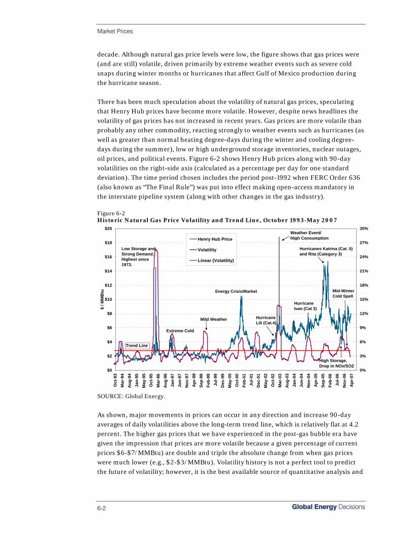
Market Prices
6-2
decade. Although natural gas price levels were low, the figure shows that gas prices were (and are still) volatile, driven primarily by extreme weather events such as severe cold snaps during winter months or hurricanes that affect Gulf of Mexico production during the hurricane season. There has been much speculation about the volatility of natural gas prices, speculating that Henry Hub prices have become more volatile. However, despite news headlines the volatility of gas prices has not increased in recent years. Gas prices are more volatile than probably any other commodity, reacting strongly to weather events such as hurricanes (as well as greater than normal heating degree-days during the winter and cooling degree-days during the summer), low or high underground storage inventories, nuclear outages, oil prices, and political events. Figure 6-2 shows Henry Hub prices along with 90-day volatilities on the right-side axis (calculated as a percentage per day for one standard deviation). The time period chosen includes the period post-1992 when FERC Order 636 (also known as “The Final Rule”) was put into effect making open-access mandatory in the interstate pipeline system (along with other changes in the gas industry). Figure 6-2 Historic Natural Gas Price Volatility and Trend Line, October 1993-May 2007
$0
$2
$4
$6
$8
$10
$12
$14
$16
$18
$20
Oct
-93
Mar
-94
Aug
-94
Jan-
95M
ay-9
5O
ct-9
5M
ar-9
6A
ug-9
6Ja
n-97
Jun-
97N
ov-9
7A
pr-9
8Se
p-98
Feb-
99Ju
l-99
Dec
-99
May
-00
Oct
-00
Feb-
01Ju
l-01
Dec
-01
May
-02
Oct
-02
Mar
-03
Aug
-03
Jan-
04Ju
n-04
Nov
-04
Apr
-05
Sep-
05Fe
b-06
Jul-0
6N
ov-0
6A
pr-0
7
$ / M
MB
tu
0%
3%
6%
9%
12%
15%
18%
21%
24%
27%
30%
Henry Hub Price
Volatility
Linear (Volatility)
Trend Line
Weather Event/High Consumption
Energy Crisis/Market
Mild Weather
Hurricanes Katrina (Cat. 5) and Rita (Category 3)
Mid-WinterCold Spell
Hurricane Lili (Cat.4)
Hurricane Ivan (Cat 3)
Extreme Cold
Low Storage and Strong Demand;Highest since 1973.
High Storage,Drop in NOx/SO2
SOURCE: Global Energy. As shown, major movements in prices can occur in any direction and increase 90-day averages of daily volatilities above the long-term trend line, which is relatively flat at 4.2 percent. The higher gas prices that we have experienced in the post-gas bubble era have given the impression that prices are more volatile because a given percentage of current prices $6-$7/MMBtu) are double and triple the absolute change from when gas prices were much lower (e.g., $2-$3/MMBtu). Volatility history is not a perfect tool to predict the future of volatility; however, it is the best available source of quantitative analysis and

Market Prices
Gas Reference Case, Fall 2007 6-3
volatility is an essential input component in the Black-Sholes pricing model in order to determine the value of options (e.g., puts and calls). When the rate of growth of net Canadian exports began to stall starting in 2000, combined with continued strong U.S. demand, gas market prices spiked, eventually reaching about $10/MMBtu in late 2000. These factors, combined with rising net gas exports to Mexico, which increased significantly in 1999 and have grown ever since, have helped to prick the gas supply bubble for good (see Figure 6-2). In the past several years, a slight reversal of net imports has occurred. Canadian net exports to the U.S. have declined while net exports to Mexico have risen, both a net loss of supply for the United States. Global Energy expects that exports to Mexico will moderate as new LNG supply to Mexico on their west coast materializes in addition to the recently completed Altamira terminal on their east coast in the Gulf of Mexico. Our current analysis for 2007 and beyond is that Canadian net exports will continue their recent trend of decline, reflecting Canadian domestic gas market growth (including oil sands), disappointing gas deliverability from the Sable Island Offshore Energy Project in the North Atlantic, and relatively stagnant Alberta production. Co-mingling regasified LNG from Canadian terminals will ease the crunch in the last years of the forecast. Figure 6-3 Net Annual Canadian and Mexican Imports
-500
0
500
1,000
1,500
2,000
2,500
3,000
3,500
4,000
1990
1992
1994
1996
1998
2000
2002
2004
2006
2008
2010
2012
2014
2016
2018
2020
2022
2024
2026
Bcf
/ Ye
ar
Net Canadian Imports
Net Mexican Imports
ForecastActual
SOURCE: Global Energy.
Market Prices
6-4
Gas Market Evolution Global Energy’s Reference Case is based on our expectations of how natural gas supply and demand factors will “play out” between 2006 and 2030.1 We characterize this forecast as our expected case, based on the best available data using a fundamental natural gas model. However, many factors could push prices higher or lower for several months or longer. The degree of inherent uncertainty about future gas market conditions such as finding and developing costs for incremental supplies, on the timing of major new infrastructure such as the number of new LNG regasification terminals, and the level of expansion and extension of the interstate pipeline network should be carefully considered. Several of these factors cannot be forecast with a high degree of confidence for even more than a few years. Much of the analysis presented in Sections 2, 3, and 4 describes how market forces have “upset” conventional views of natural gas markets in North America. In Global Energy’s opinion, the North American natural gas market is transforming from a continental gas market—mostly disconnected from world LNG trade—to a more integrated global gas market with increasing dependence on various global LNG suppliers. This transformation has begun in part due to rising domestic production costs and land-use restrictions, decreasing LNG costs, and the impending growth in gas demand for electric power generation. Global Energy believes that market “transformation” has already begun. What evidence is available to support this assertion? First, development and production costs for conventional gas in North America have risen significantly in recent years, breaking with historical downward cost trends. This is significant because until the last few years, reductions in finding and developing costs due largely to technological improvements have reduced overall costs and increased wellhead gas deliverability, or at least stabilized production even with the declining quality and size of incremental gas reserves. Recently, the rise in indigenous gas costs coupled with a decline in LNG costs (due to technology improvements) has made LNG a highly competitive fuel option for North America. Second, increased industry concentration of the new “Super Majors” brought about by industry consolidation during the 1990s (and still under way) when industry return on capital employed was at an all time low, has reduced competition and exploration and development budgets—often through workforce reductions and through economies of scale and scope. In the recent commodity cycle, many producers have also shown less willingness to reinvest cash flow (especially in North America) in favor of shareholder interests and of better overseas opportunities. Third, deregulation of the wholesale electric power sector and the resulting gas-fired merchant overbuild has set in motion significant future gas demand growth. As discussed
1 Note, fundamental supply, demand, and transportation analysis was only provided through 2027. Projections through 2032 were made by using linear extrapolation of trends. All fundamental analysis through 2033 will be provided starting with the Spring 2008 Reference Case.
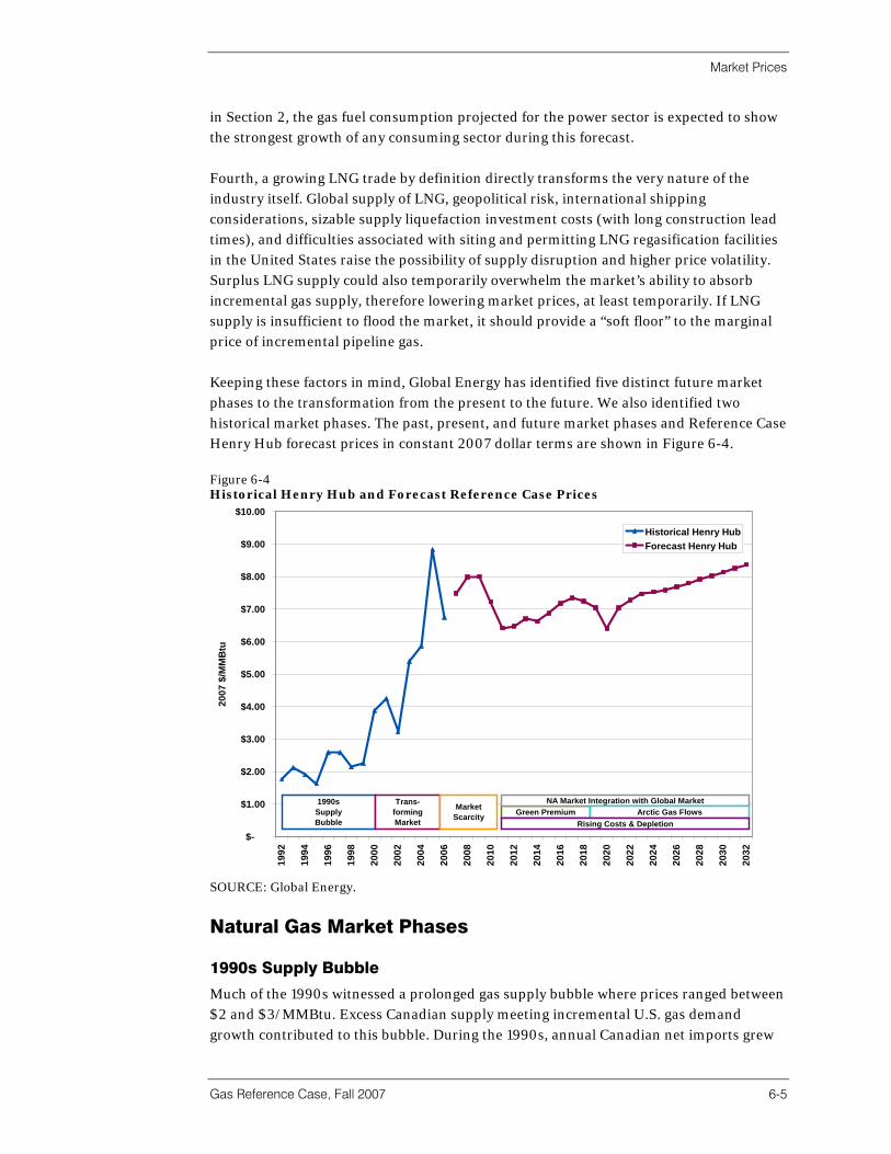
Market Prices
Gas Reference Case, Fall 2007 6-5
in Section 2, the gas fuel consumption projected for the power sector is expected to show the strongest growth of any consuming sector during this forecast. Fourth, a growing LNG trade by definition directly transforms the very nature of the industry itself. Global supply of LNG, geopolitical risk, international shipping considerations, sizable supply liquefaction investment costs (with long construction lead times), and difficulties associated with siting and permitting LNG regasification facilities in the United States raise the possibility of supply disruption and higher price volatility. Surplus LNG supply could also temporarily overwhelm the market’s ability to absorb incremental gas supply, therefore lowering market prices, at least temporarily. If LNG supply is insufficient to flood the market, it should provide a “soft floor” to the marginal price of incremental pipeline gas. Keeping these factors in mind, Global Energy has identified five distinct future market phases to the transformation from the present to the future. We also identified two historical market phases. The past, present, and future market phases and Reference Case Henry Hub forecast prices in constant 2007 dollar terms are shown in Figure 6-4. Figure 6-4 Historical Henry Hub and Forecast Reference Case Prices
$-
$1.00
$2.00
$3.00
$4.00
$5.00
$6.00
$7.00
$8.00
$9.00
$10.00
1992
1994
1996
1998
2000
2002
2004
2006
2008
2010
2012
2014
2016
2018
2020
2022
2024
2026
2028
2030
2032
2007
$/M
MB
tu
Historical Henry HubForecast Henry Hub
1990s Supply Bubble
Trans-formingMarket
Market Scarcity Green Premium
NA Market Integration with Global MarketArctic Gas Flows
Rising Costs & Depletion
SOURCE: Global Energy.
Natural Gas Market Phases 1990s Supply Bubble
Much of the 1990s witnessed a prolonged gas supply bubble where prices ranged between $2 and $3/MMBtu. Excess Canadian supply meeting incremental U.S. gas demand growth contributed to this bubble. During the 1990s, annual Canadian net imports grew
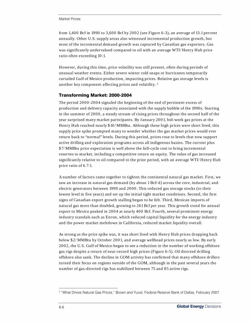
Market Prices
6-6
from 1,400 Bcf in 1990 to 3,600 Bcf by 2002 (see Figure 6-3), an average of 13.1 percent annually. Other U.S. supply areas also witnessed incremental production growth, but most of the incremental demand growth was captured by Canadian gas exporters. Gas was significantly undervalued compared to oil with an average WTI/Henry Hub price ratio often exceeding 10:1. However, during this time, price volatility was still present, often during periods of unusual weather events. Either severe winter cold snaps or hurricanes temporarily curtailed Gulf of Mexico production, impacting prices. Relative gas storage levels is another key component affecting prices and volatility. 2 Transforming Market: 2000-2004
The period 2000-2004 signaled the beginning of the end of persistent excess of production and delivery capacity associated with the supply bubble of the 1990s. Starting in the summer of 2000, a steady stream of rising prices throughout the second half of the year surprised many market participants. By January 2001, bid-week gas prices at the Henry Hub reached nearly $10/MMBtu. Although these high prices were short lived, this supply price spike prompted many to wonder whether the gas market prices would ever return back to “normal” levels. During this period, prices rose to levels that now support active drilling and exploration programs across all indigenous basins. The current plus $7/MMBtu price expectation is well above the full-cycle cost to bring incremental reserves to market, including a competitive return on equity. The value of gas increased significantly relative to oil compared to the prior period, with an average WTI/Henry Hub price ratio of 6.7:1. A number of factors came together to tighten the continental natural gas market. First, we saw an increase in natural gas demand (by about 1 Bcf/d) across the core, industrial, and electric generators between 1999 and 2000. This reduced gas storage stocks (to their lowest level in five years) and set up the initial tight market conditions. Second, the first signs of Canadian export growth stalling began to be felt. Third, Mexican imports of natural gas more than doubled, growing to 261 Bcf per year. This growth trend for annual export to Mexico peaked in 2004 at nearly 400 Bcf. Fourth, several prominent energy industry scandals such as Enron, which reduced capital liquidity for the energy industry and the power market meltdown in California, reduced market liquidity overall. As strong as the price spike was, it was short lived with Henry Hub prices dropping back below $2/MMBtu by October 2001, and average wellhead prices nearly as low. By early 2002, the U.S. Gulf of Mexico began to see a reduction in the number of working offshore gas rigs despite a return of near-record high prices (Figure 6-5). Oil directed drilling offshore also sank. The decline in GOM activity has confirmed that many offshore drillers turned their focus on regions outside of the GOM, although in the past several years the number of gas-directed rigs has stabilized between 75 and 85 active rigs.
2 “What Drives Natural Gas Prices,” Brown and Yucel, Federal Reserve Bank of Dallas, February 2007.
Market Prices
Gas Reference Case, Fall 2007 6-7
Figure 6-5 Gulf of Mexico (GOM) Working Gas Rigs and Wellhead Price (Monthly Averages)
0
20
40
60
80
100
120
140
Jan-
00
Jul-0
0
Jan-
01
Jul-0
1
Jan-
02
Jul-0
2
Jan-
03
Jul-0
3
Jan-
04
Jul-0
4
Jan-
05
Jul-0
5
Jan-
06
Jul-0
6
Jan-
07
Jul-0
7
GO
M W
orki
ng G
as R
ig C
ount
$0
$2
$4
$6
$8
$10
$12
$14
$ pe
r Mcf
Gas Wellhead Price
GOM Gas Rigs
Hurricanes Katrina and Rita, along with subsequent repair of damaged rotary rigs, cut the working rig count and gas production by more than 50%.
SOURCE: Baker Hughes, EIA, and Global Energy.
Market Scarcity: 2005-2008
At the present time, the market psychology is extremely bullish for prices as witnessed by the NYMEX gas forward strip as of mid-March 2007. The entire summer of 2007 NYMEX is over $8/dth, with December 2007 through March 2008 prices near $10/dth. The run-up to record high world oil prices since 2003 has boosted confidence in this view, as did the perception that repeated hurricane damage in a particularly vulnerable Gulf of Mexico production region could occur. In our analysis the current period and the previous Transforming Market period confirmed: • Maintenance of crude price sympathy - the projection of an average WTI/HH price
ratio during this period of 7.5 maintains much of the increased value of gas relative to oil gained in the prior period;
• Increased world tension and a “risk premium” or “security premium” built into petroleum prices;
• Recognition of the rise in global prices of hydrocarbon fuels (crude oil products, LNG, coal) due to strong demand growth in several large developing countries, especially China and India, a “scarcity premium”;
• Rising gas finding and development (F&D) costs across North America; • The partial decline in drilling in the Gulf of Mexico despite record high prices; and • Pre-determined rising electric power fuel demand due to the current generator
overbuild. The combination of these market factors has resulted in a permanent rise in gas prices, rather than prices spiking up and then returning to lower, long-run equilibrium levels.

Market Prices
6-8
Presently, crude price sympathy, security and scarcity premiums, and a very bullish market perception have caused Henry Hub prices to trade well above long-run replacement cost. Further, during the next 48-month period, Global Energy’s price forecast takes these factors into account. Global Energy notes that recent oil and gas profitability is well above long-term industry norms, which we believe supports our view that increases in finding and developing costs, which have risen, have not risen nearly as much as have gas prices. We expect oil and gas producers to continue to increase their capital spending programs in the coming years in an attempt to grow production volumes. But given barriers to entry, the long lead times necessary to bring new gas reserves into production, and the high decline rate of both current producing wells and of expected lower-quality new wells, actual growth in production, if at all, should be gradual at 1 to 2 percent per year. LNG Renaissance: 2009-2015
In a previous Gas Reference Case report released in early 2005, Global Energy considered an “LNG Renaissance” period materializing during the 2008-2012 time frame. Our current view has not changed in this regard and, in fact, may be vindicated given the record volumes of LNG that entered the U.S. in the first seven months of 2007. The level of LNG development activity now under way in North America has only bolstered our view that LNG will grow in importance in the coming years. As of September 2007, six LNG import terminals were currently operating in the United States and Mexico and our research indicates that five more plants are under construction in the U.S. with on line dates on or before 2010. Two additional facilities—one each in Canada and Mexico—are also under construction and are expected to impact the continental gas trade by 2008. Two existing terminals are also undergoing expansion. The Altamira receiving terminal in Mexico became fully operational at the end of 2006. While this plant is expected to supply the domestic Mexican market, it could reduce some of the exports to that country starting as early as next year. In addition to these LNG plants developments, at least 16 other plants have been permitted (see Section 4). And in addition to these, over 40 more LNG regasification projects are currently being planned by developers with on line dates before 2015. We recognize the difficulty in permitting and constructing these facilities and have significantly limited the number of facilities assumed to be built in our Reference Case during this time frame. NIMBY or siting issues, access to firm (dedicated) and spot (merchant) LNG supply, contractual issues over the redirection of LNG cargoes, interchangeability issues (e.g., Wobbe Index), and the available new LNG tankers will reduce and delay the volumes of LNG that can enter North America over this period. And in the Reference Case forecast we have constrained the send-out rate and annual capacity utilization rate of LNG facilities to reflect these market conditions (see Section 4 for more details). Of course, market uncertainty and the direction of price continue to grow as the analysis moves further out in time; however, with North America’s growing dependence on LNG
Market Prices
Gas Reference Case, Fall 2007 6-9
comes increased global risk factors. We simply do not know how development policies, economic growth, and LNG demand will materialize in Asian and European markets five to ten years out. We also do not know how much incremental LNG supply will become available and under what terms. But the continuous rise in gas demand for power generation, relatively flat continental supply with rising production costs due to depletion, coupled with rising dependence on foreign LNG supply and its linkage to global oil prices mean external market forces will grow in importance and possibly dominate continental gas markets. During this period the price of natural gas declines moderately from approximately $8.00/MMBtu to $6.90/MMBtu, as the result of increased LNG supply taking the price set by the marginal cost of indigenous gas. Although gas prices decrease, crude oil is falling faster and therefore reflects a higher value of gas compared to oil with an average WTI/HH price ratio decreasing from 8.4:1 to 7.5:1 Arctic Gas Flows: 2015-2025
Due to high infrastructure costs and political/regulatory issues—both national and international that affect when Arctic gas pipelines can begin construction, the delivery volumes, locations, and in-service dates, Global Energy expects that gas from Alaska will not begin to flow until 2020. In our analysis we have assumed that Mackenzie Valley gas will come on line before Alaska by approximately two years. Alaska is forecast to come on line in 2020 at 4.5 Bcf/d, and then ramp up to full production (6.5 Bcf/d) by 2025. In Canada, delays in obtaining final approval from one Indian nation (Deh Cho) make the actual on line year uncertain. It is widely believed that the Mackenzie Valley-Beaufort Sea reserves can economically support 1.2 Bcf/d in 2018, then ramping up to 2.4 Bcf/day. Detailed engineering analysis is currently under way to determine the final routing and design details. A cost revision in mid-March increased the capital estimate to $13.65 billion and recently to $15.4 billion. During this period, North America will again see the lower gas prices under Global Energy’s Reference Case forecast caused by the entry of very large volumes of Arctic gas from Alaska and Canada. Additional LNG volumes also materialize during the last 10 forecast years as growth in gas demand—especially for electric generation—will continue to pressure natural gas prices and provide the necessary market incentives for continued LNG development across the continent and globally. Gas prices drop from approximately $7.35/MMBtu to $6.45/MMBtu in 2020 due to the increased supply, then rise to $7.56/MMBtu by the end of this period. The value of gas gains somewhat along with the volumes of Arctic gas; the average WTI/HH price ration declines from a high of 8.1:1 to 7.25:1 during this period.
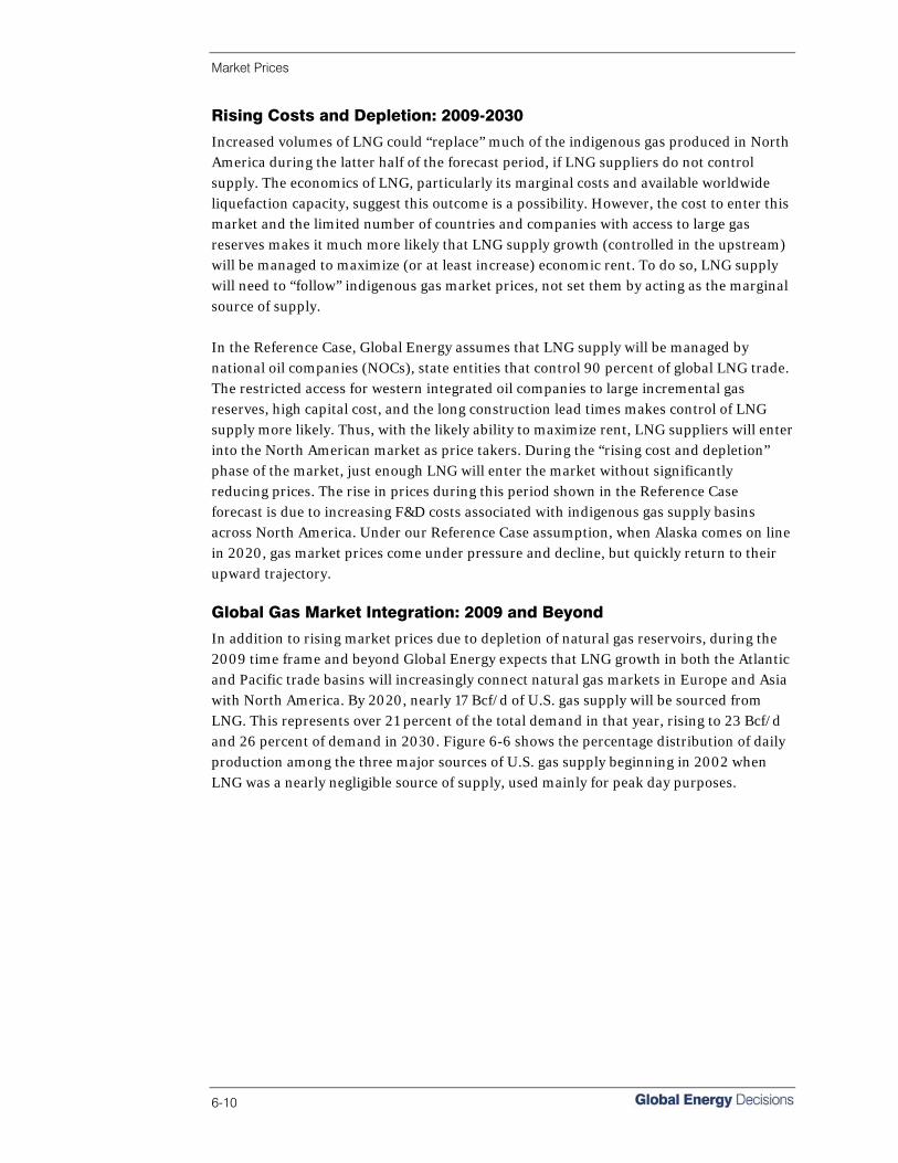
Market Prices
6-10
Rising Costs and Depletion: 2009-2030
Increased volumes of LNG could “replace” much of the indigenous gas produced in North America during the latter half of the forecast period, if LNG suppliers do not control supply. The economics of LNG, particularly its marginal costs and available worldwide liquefaction capacity, suggest this outcome is a possibility. However, the cost to enter this market and the limited number of countries and companies with access to large gas reserves makes it much more likely that LNG supply growth (controlled in the upstream) will be managed to maximize (or at least increase) economic rent. To do so, LNG supply will need to “follow” indigenous gas market prices, not set them by acting as the marginal source of supply. In the Reference Case, Global Energy assumes that LNG supply will be managed by national oil companies (NOCs), state entities that control 90 percent of global LNG trade. The restricted access for western integrated oil companies to large incremental gas reserves, high capital cost, and the long construction lead times makes control of LNG supply more likely. Thus, with the likely ability to maximize rent, LNG suppliers will enter into the North American market as price takers. During the “rising cost and depletion” phase of the market, just enough LNG will enter the market without significantly reducing prices. The rise in prices during this period shown in the Reference Case forecast is due to increasing F&D costs associated with indigenous gas supply basins across North America. Under our Reference Case assumption, when Alaska comes on line in 2020, gas market prices come under pressure and decline, but quickly return to their upward trajectory. Global Gas Market Integration: 2009 and Beyond
In addition to rising market prices due to depletion of natural gas reservoirs, during the 2009 time frame and beyond Global Energy expects that LNG growth in both the Atlantic and Pacific trade basins will increasingly connect natural gas markets in Europe and Asia with North America. By 2020, nearly 17 Bcf/d of U.S. gas supply will be sourced from LNG. This represents over 21 percent of the total demand in that year, rising to 23 Bcf/d and 26 percent of demand in 2030. Figure 6-6 shows the percentage distribution of daily production among the three major sources of U.S. gas supply beginning in 2002 when LNG was a nearly negligible source of supply, used mainly for peak day purposes.
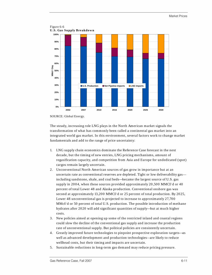
Market Prices
Gas Reference Case, Fall 2007 6-11
Figure 6-6 U.S. Gas Supply Breakdown
0%
10%
20%
30%
40%
50%
60%
70%
80%
90%
100%
2002 2007 2010 2015 2020 2025 2030
MM
cf /
Day
U.S. Production Net Pipeline Imports LNG Imports
SOURCE: Global Energy.
The steady, increasing role LNG plays in the North American market signals the transformation of what has commonly been called a continental gas market into an integrated world gas market. In this environment, several factors work to change market fundamentals and add to the range of price uncertainty: 1. LNG supply chain economics dominate the Reference Case forecast in the next
decade, but the timing of new entries, LNG pricing mechanisms, amount of regasification capacity, and competition from Asia and Europe for undedicated (spot) cargos remain largely uncertain.
2. Unconventional North American sources of gas grow in importance but at an uncertain rate as conventional reserves are depleted. Tight or low deliverability gas—including sandstone, shale, and coal beds—became the largest source of U.S. gas supply in 2004, when these sources provided approximately 20,500 MMCf/d or 40 percent of total Lower 48 and Alaska production. Conventional onshore gas was second at approximately 13,200 MMCf/d or 25 percent of total production. By 2025, Lower 48 unconventional gas is projected to increase to approximately 27,700 MMcf/d or 50 percent of total U.S. production. The possible introduction of methane hydrates after 2020 will add significant quantities of supply—but at much higher costs.
3. New policies aimed at opening up some of the restricted inland and coastal regions could slow the decline of the conventional gas supply and increase the production rate of unconventional supply. But political policies are consistently uncertain.
4. Greatly improved future technologies to pinpoint prospective exploration targets—as well as advanced development and production technologies—are likely to reduce wellhead costs, but their timing and impacts are uncertain.
5. Sustainable reductions in long-term gas demand may reduce pricing pressure.

Market Prices
6-12
Key North American Market Prices Figure 6-7 shows relative changes in supply area prices for six market hubs including the Henry Hub. During most of the forecast period the relative position of prices at each hub compared to the Henry Hub remains relatively intact. In one of our previous Natural Gas Reference Case report (released in 2005) we noted that basis differential reversals were more common. In that analysis, we concluded that that cause was attributed to large LNG growth in the Gulf of Mexico, which depressed Henry Hub gas prices relative to many downstream market hubs. Our reasoning for this was that siting difficulties outside of the Gulf would preclude LNG facility developments on both the Atlantic and Pacific coasts. Since that report’s release, we continue to believe that siting will be easier in the Gulf of Mexico. In fact, six new construction projects have commenced in the Gulf of Mexico: Freeport, Texas; Cameron, Louisiana; Sabine Pass, Louisiana; Golden Pass, Texas; Corpus Christi, Texas; and Energia Costa Azul, Mexico. We still believe that the relative ease of siting and of processing LNG compositions combined with the desire to “backfill” the existing long-haul gas pipeline network, along with the desire of local government to increase their tax base, provide compelling reasons to locate the majority of new LNG regasification facility along the GOM. We now expect that concurrent with progress in the GOM there will be steady and measured progress elsewhere in building LNG terminals closer to other major market hubs. This view has been confirmed by progress made to date. The issue of LNG composition interchangeability is being addressed and will be resolved at FERC and in other regulatory venues. Additional signs of non-GOM progress include: • The likelihood of one additional LNG facility in Atlantic Canada; • The likelihood of a terminal in British Columbia; • Construction now well under way in Baja Mexico; • Large scale expansions at existing U.S. Atlantic Coast regasification facilities; and • The possibility of several greenfield facilities on or off both the Atlantic and Pacific
coasts. Basis spreads are forecast to narrow somewhat in the 2008-2011 period coinciding with the end of the market scarcity period and the initial expansion of LNG supply during the LNG Renaissance period. Also, by 2014, the price at the AECO hub begins to separate further from other major market hubs. This is caused by the influx of large volumes of frontier Arctic gas entering the Alberta market for redelivery to the Lower 48 markets. In our analysis and modeling, we found significant export constraints along several export corridors by which Arctic gas is redelivered away from the AECO hub. In addition to the market prices shown below, the data appendix provides prices on a monthly and annual base for the Reference Case forecast for 36 market hubs.
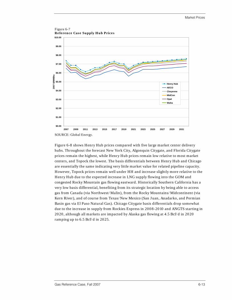
Market Prices
Gas Reference Case, Fall 2007 6-13
Figure 6-7 Reference Case Supply Hub Prices
$0.00
$1.00
$2.00
$3.00
$4.00
$5.00
$6.00
$7.00
$8.00
$9.00
$10.00
2007 2009 2011 2013 2015 2017 2019 2021 2023 2025 2027 2029 2031
2007
$/M
MB
tu
Henry HubAECO
CheyenneMidConOpal
Waha
SOURCE: Global Energy.
Figure 6-8 shows Henry Hub prices compared with five large market center delivery hubs. Throughout the forecast New York City, Algonquin Citygate, and Florida Citygate prices remain the highest, while Henry Hub prices remain low relative to most market centers, and Topock the lowest. The basis differentials between Henry Hub and Chicago are essentially the same indicating very little market value for related pipeline capacity. However, Topock prices remain well under HH and increase slightly more relative to the Henry Hub due to the expected increase in LNG supply flowing into the GOM and congested Rocky Mountain gas flowing eastward. Historically Southern California has a very low basis differential, benefiting from its strategic location by being able to access gas from Canada (via Northwest/Malin), from the Rocky Mountains/Midcontinent (via Kern River), and of course from Texas/New Mexico (San Juan, Anadarko, and Permian Basin gas via El Paso Natural Gas). Chicago Citygate basis differentials drop somewhat due to the increase in supply from Rockies Express in 2008-2010 and ANGTS starting in 2020, although all markets are impacted by Alaska gas flowing at 4.5 Bcf/d in 2020 ramping up to 6.5 Bcf/d in 2025.
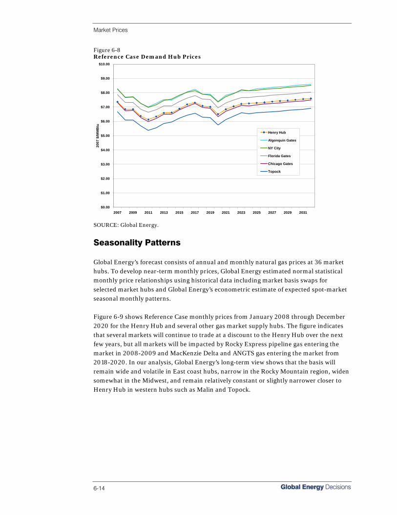
Market Prices
6-14
Figure 6-8 Reference Case Demand Hub Prices
$0.00
$1.00
$2.00
$3.00
$4.00
$5.00
$6.00
$7.00
$8.00
$9.00
$10.00
2007 2009 2011 2013 2015 2017 2019 2021 2023 2025 2027 2029 2031
2007
$/M
MB
tu
Henry Hub
Algonquin Gates
NY City
Florida Gates
Chicago Gates
Topock
SOURCE: Global Energy.
Seasonality Patterns Global Energy’s forecast consists of annual and monthly natural gas prices at 36 market hubs. To develop near-term monthly prices, Global Energy estimated normal statistical monthly price relationships using historical data including market basis swaps for selected market hubs and Global Energy’s econometric estimate of expected spot-market seasonal monthly patterns. Figure 6-9 shows Reference Case monthly prices from January 2008 through December 2020 for the Henry Hub and several other gas market supply hubs. The figure indicates that several markets will continue to trade at a discount to the Henry Hub over the next few years, but all markets will be impacted by Rocky Express pipeline gas entering the market in 2008-2009 and MacKenzie Delta and ANGTS gas entering the market from 2018-2020. In our analysis, Global Energy’s long-term view shows that the basis will remain wide and volatile in East coast hubs, narrow in the Rocky Mountain region, widen somewhat in the Midwest, and remain relatively constant or slightly narrower closer to Henry Hub in western hubs such as Malin and Topock.
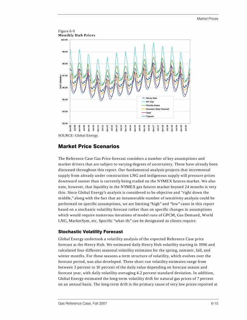
Market Prices
Gas Reference Case, Fall 2007 6-15
Figure 6-9 Monthly Hub Prices
$3.00
$4.00
$5.00
$6.00
$7.00
$8.00
$9.00
$10.00
Jan-
08
Jul-0
8
Jan-
09
Jul-0
9
Jan-
10
Jul-1
0
Jan-
11
Jul-1
1
Jan-
12
Jul-1
2
Jan-
13
Jul-1
3
Jan-
14
Jul-1
4
Jan-
15
Jul-1
5
Jan-
16
Jul-1
6
Jan-
17
Jul-1
7
Jan-
18
Jul-1
8
Jan-
19
Jul-1
9
Jan-
20
Jul-2
0
2007
$/M
MB
tu
Henry HubNY CityFlorida GatesHouston Ship ChannelOpalTopock
SOURCE: Global Energy.
Market Price Scenarios The Reference Case Gas Price forecast considers a number of key assumptions and market drivers that are subject to varying degrees of uncertainty. These have already been discussed throughout this report. Our fundamental analysis projects that incremental supply from already under construction LNG and indigenous supply will pressure prices downward sooner than is currently being traded on the NYMEX futures market. We also note, however, that liquidity in the NYMEX gas futures market beyond 24 months is very thin. Since Global Energy’s analysis is considered to be objective and “right down the middle,” along with the fact that an innumerable number of sensitivity analysis could be performed on specific assumptions, we are limiting “high” and “low” cases in this report based on a stochastic volatility forecast rather than on specific changes in assumptions which would require numerous iterations of model runs of GPCM, Gas Demand, World LNG, MarketSym, etc. Specific “what-ifs” can be designated as clients require. Stochastic Volatility Forecast
Global Energy undertook a volatility analysis of the expected Reference Case price forecast at the Henry Hub. We estimated daily Henry Hub volatility starting in 1996 and calculated four different seasonal volatility estimates for the spring, summer, fall, and winter months. For these seasons a term structure of volatility, which evolves over the forecast period, was also developed. These short run volatility estimates range from between 3 percent to 10 percent of the daily value depending on forecast season and forecast year, with daily volatility averaging 4.2 percent standard deviation. In addition, Global Energy estimated the long-term volatility drift for natural gas prices of 7 percent on an annual basis. The long-term drift is the primary cause of very low prices reported at
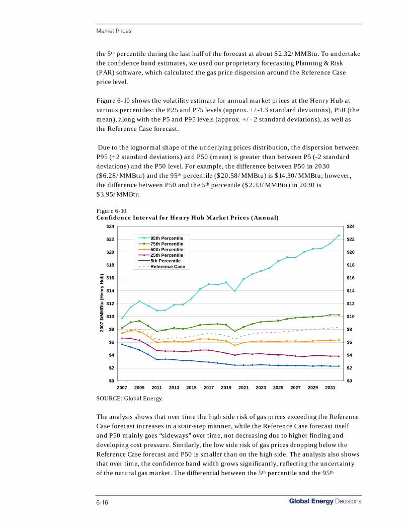
Market Prices
6-16
the 5th percentile during the last half of the forecast at about $2.32/MMBtu. To undertake the confidence band estimates, we used our proprietary forecasting Planning & Risk (PAR) software, which calculated the gas price dispersion around the Reference Case price level. Figure 6-10 shows the volatility estimate for annual market prices at the Henry Hub at various percentiles: the P25 and P75 levels (approx. +/-1.3 standard deviations), P50 (the mean), along with the P5 and P95 levels (approx. +/- 2 standard deviations), as well as the Reference Case forecast. Due to the lognormal shape of the underlying prices distribution, the dispersion between P95 (+2 standard deviations) and P50 (mean) is greater than between P5 (-2 standard deviations) and the P50 level. For example, the difference between P50 in 2030 ($6.28/MMBtu) and the 95th percentile ($20.58/MMBtu) is $14.30/MMBtu; however, the difference between P50 and the 5th percentile ($2.33/MMBtu) in 2030 is $3.95/MMBtu. Figure 6-10 Confidence Interval for Henry Hub Market Prices (Annual)
$0
$2
$4
$6
$8
$10
$12
$14
$16
$18
$20
$22
$24
2007 2009 2011 2013 2015 2017 2019 2021 2023 2025 2027 2029 2031
200
7 $/
MM
Btu
(Hen
ry H
ub)
$0
$2
$4
$6
$8
$10
$12
$14
$16
$18
$20
$22
$24
95th Percentile75th Percentile50th Percentile25th Percentile5th PercentileReference Case
SOURCE: Global Energy.
The analysis shows that over time the high side risk of gas prices exceeding the Reference Case forecast increases in a stair-step manner, while the Reference Case forecast itself and P50 mainly goes “sideways” over time, not decreasing due to higher finding and developing cost pressure. Similarly, the low side risk of gas prices dropping below the Reference Case forecast and P50 is smaller than on the high side. The analysis also shows that over time, the confidence band width grows significantly, reflecting the uncertainty of the natural gas market. The differential between the 5th percentile and the 95th
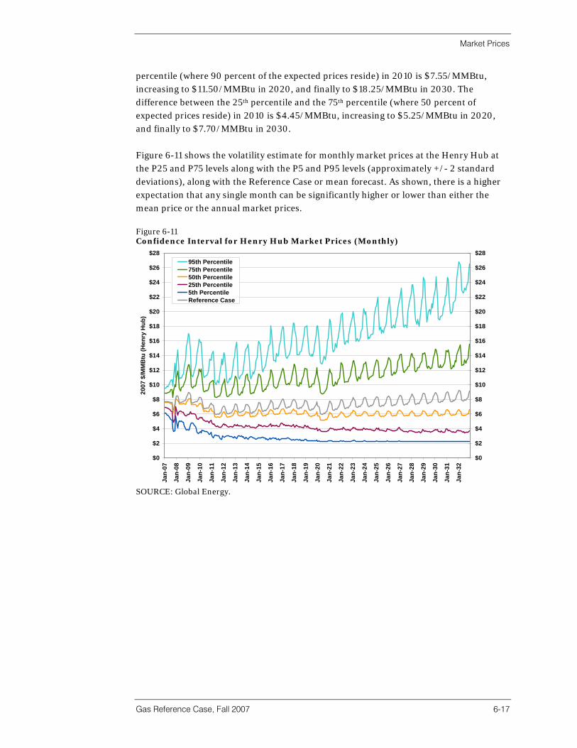
Market Prices
Gas Reference Case, Fall 2007 6-17
percentile (where 90 percent of the expected prices reside) in 2010 is $7.55/MMBtu, increasing to $11.50/MMBtu in 2020, and finally to $18.25/MMBtu in 2030. The difference between the 25th percentile and the 75th percentile (where 50 percent of expected prices reside) in 2010 is $4.45/MMBtu, increasing to $5.25/MMBtu in 2020, and finally to $7.70/MMBtu in 2030. Figure 6-11 shows the volatility estimate for monthly market prices at the Henry Hub at the P25 and P75 levels along with the P5 and P95 levels (approximately +/- 2 standard deviations), along with the Reference Case or mean forecast. As shown, there is a higher expectation that any single month can be significantly higher or lower than either the mean price or the annual market prices. Figure 6-11 Confidence Interval for Henry Hub Market Prices (Monthly)
$0
$2
$4
$6
$8
$10
$12
$14
$16
$18
$20
$22
$24
$26
$28
Jan-
07
Jan-
08
Jan-
09
Jan-
10
Jan-
11
Jan-
12
Jan-
13
Jan-
14
Jan-
15
Jan-
16
Jan-
17
Jan-
18
Jan-
19
Jan-
20
Jan-
21
Jan-
22
Jan-
23
Jan-
24
Jan-
25
Jan-
26
Jan-
27
Jan-
28
Jan-
29
Jan-
30
Jan-
31
Jan-
32
2007
$/M
MB
tu (H
enry
Hub
)
$0
$2
$4
$6
$8
$10
$12
$14
$16
$18
$20
$22
$24
$26
$2895th Percentile75th Percentile50th Percentile25th Percentile5th PercentileReference Case
SOURCE: Global Energy.


Section 7 | Methodology


Methodology
Gas Reference Case, Fall 2007 7-1
Introduction This report section describes the methodology used to produce Global Energy’s natural gas price forecast. Our analysis of natural gas markets includes a fundamental market assessment of: • Natural gas prices; • Basis differentials; • Natural gas transportation; • Storage analysis; • Basin level gas supply economics; • LNG; • Pipeline and liquefied natural gas imports; and • Natural gas demand for the residential, commercial, industrial, and electric
generation sectors. The fundamental gas model used to prepare Global Energy’s forecast is RBAC’s GPCM gas model. The model forecasts natural gas production, interstate and intrastate transportation, storage, and prices necessary to meet demand by sector. GPCM simulates regional interactions between supply, transportation, storage, and demand to determine market clearing prices. Projected fuel prices and forecast gas demand for electric generation are integrated with Global Energy’s North American Reference Case modeling framework (Figure 7-1).1
Figure 7-1 Generalized Equilibrium Solution Example
Demand
EmissionPrice
Forecast
Price
Oil Model
Coal Model
GasModel
ReferenceCase
ForecastPrice Price
Price
Price
Demand
PricePrice
Oil Model
Demand
Demand
EmissionPrice
Forecast
Price
Oil Model
Coal Model
GasModel
ReferenceCase
ForecastPrice Price
Price
Price
Demand
PricePrice
Oil Model
Demand
SOURCE: Global Energy.
1 The North American Reference Case is a 25-year price forecast of 76 competitive power markets across every North American Electric Reliability Council region. These forecasts are updated twice per year.
Methodology
7-2
Within this modeling framework, the interaction of coal prices and demand, oil prices, and emission allowance credits and their cost are integrated. This approach includes fuel switching and substitution effects across energy commodities and substitutes. In particular, gas consumed by power generators as economically dispatched to meet load is recorded and fed as an input into the GPCM model (along with other sources of demand) to produce the gas price forecast. Various model components are simulated with the key forecast results (prices or demand) fed back into the other models. Natural gas demand for residential, commercial, and industrial sources is derived using econometric equations that measure monthly sector gas demand by individual state and province. The variables used include heating and cooling degree days, gross state product, market price of natural gas, income, non-farm payroll, and seasonal dummy variables representing each month of the year. To forecast electric generator gas consumption, Global Energy used forecast gas consumption resulting from its Spring 2007 Power Reference Case market forecast for North America. The model used to prepare the forecast is Market Analytics, formerly known as PROSYM (or MARKETSYM). For each Power Market region (76 in all) the model considers: • Individual power plant characteristics including heat rates, start-up costs, ramp rates,
and other technical characteristics of plants; • Transmission line interconnections, ratings, losses, and wheeling rates; • Forecasts of resource additions and fuel costs over time; • Forecasts of loads for each utility or load serving entity in the region; and • The cost and availability of fuels that supply the plants. Market Analytics simulates the operation of individual generators, utilities, and control areas to meet fluctuating loads within the region with hourly detail. The model is based on a zonal approach where market areas (zones) are delineated by critical transmission constraints. The simulation is based on a mathematical objective function that minimizes the cost of serving load within the modeled electric system subject to meeting load, a number of operational constraints, as well as the assumed strategic behavior (bidding) of market participants. Monte Carlo analysis is employed to incorporate individual unit forced outages. The result is a long-term price forecast that allows existing and new generators to recover all short- and long-term costs (including financing costs) from the market. The model simulates price formation in competitive markets using a least cost approach with an explicitly defined scarcity bidding behavior. Three fundamental principles guide the forecast development: • Maintain sufficient reliability in all market areas; • In the short term, benchmark the model against observed historical market prices
and market heat rates; and
Methodology
Gas Reference Case, Fall 2007 7-3
• In the long term, allow new capacity to recover all costs, including fixed and financing costs from the energy market.
Power plant resource expansions consist of currently announced and under construction plants and long-term generic economic entry units. The long-run equilibrium involves simulated plant expansion when such expansions would be profitable in the sense of meeting reasonable financial performance targets. This is the economists’ sense of zero economic profit but does not mean that investors add plants without expecting a reasonable return. Global Energy focuses on a balanced entry of base loaded and peaking generation to maintain system reliability while allowing profitable entry of new capacity. Base loaded capacity determines the pace of construction and, generally, prices in the market. Peaking capacity is entered to ensure sufficient reliability. Profitability of this peaking capacity is determined not only by the simulated deterministic prices but also by volatility and the likelihood of failure of other generation and transmission facilities, and is treated somewhat differently.
Base Loaded Capacity The simulation for a given year is an iterative procedure. First, initial expansion cases are identified for the next few years using regional reserve margin criteria and guidelines. This includes new generation technology based on the vintage of the unit. Construction costs are identified, taking into account regional variations in such costs. Operation of the regional electric system is simulated to determine forecast energy prices for one year, and the net revenue performance of new capacity additions. If this net revenue falls below the target level for new capacity in a transmission area, the unit is tentatively removed from the simulation. If the net revenue exceeds the target, then an additional simulated unit is added. The process continues until an equilibrium expansion plan for that year is reached. In practice, further complexity is added by considering: • Zonal interdependence. Plant additions or removals in one transmission area or
zone typically change outcomes in nearby zones. Thus, an iteration typically involves several additions and subtractions of generation;
• Multiple generator types. The conditions that support a base loaded combined cycle unit are different from those that support a gas turbine peaker and additions and therefore need to be carefully balanced. For instance, more peaking capacity may be necessary if changes in base load capacity have a dramatic impact on profitability in the zone. Conversely, more base load capacity may be called for if peakers run at high capacity factors and/or show very limited profitability; and
• Lack of equilibrium expansion plan. Returns may be too high in a given year if no new capacity is added and too low if capacity is added. Therefore, a long-run forecast tends to be lumpy in price.

Methodology
7-4
Global Energy’s first-cut approach to modeling peaking facilities involves the addition of new units to maintain sufficient capacity reserve margin. Reserve margin targets are set for each region, typically in the range of 12 to 20 percent. If reserve margins were to drop too low, then contingent events (such as failure of generating or transmission equipment) may result in a substantial likelihood of a loss of load and/or electricity price spikes. Figure 7-2 shows the array of inputs to outputs that are captured by each forecasting model used to prepare the integrated forecast. For example, generator consumption for fuel is endogenously determined through Electric Modeling (Market Analytics) and subsequently fed as an input into GPCM (along with sector gas demand) to develop an integrated gas price forecast. The figure below shows that in addition to gas, coal and emission allowances are treated in a similar manner. Figure 7-2 Modeling Framework Inputs and Outputs
InputInputInputInputOutputIndirectInput
IndirectInput
IndirectInput
Emissions Modeling
IndirectInputInputIndirect
InputIndirect
InputInputOutputInputIndirectInput
Coal Modeling
IndirectInput
IndirectInput
IndirectInput
IndirectInput
IndirectInput
IndirectInputOutputInputOil
Modeling
IndirectInput
IndirectInput
IndirectInputInputIndirect
InputIndirect
InputInputOutputGas Modeling
OutputOutputOutputOutputInputInputInputInputElectricity Modeling
Emission Allowances
UsedCoalFuel OilGasAllowance
PricesCoal
PricesFuel Oil Prices
Gas Prices
Generator ConsumptionForecasting Model Inputs and Outputs
SOURCE: Global Energy.
Input data used in Global Energy’s GPCM specification is prepared using Global Energy Intelligence’s Velocity Suite dataset along with the GPCM gas transportation network.
Data Sources Global Energy uses a comprehensive collection of data sources, including important industry and inter-organizational relationships, to create a robust dataset for modeling the North American natural gas market. The remainder of this section outlines the data sources for the primary modeling areas including supply, infrastructure, and demand.
Methodology
Gas Reference Case, Fall 2007 7-5
Supply Global Energy uses supply data as reported by RBAC, the United States Geological Survey (USGS), Petro Data Source, the National Petroleum Council (NPC), the Potential Gas Committee (PGC), CERI (Canadian Energy Research Institute), and the National Energy Board of Canada (NEB). These data sources are used as a starting point for creating the Global Energy supply outlook. The Petro Data Source data that is reported by basin and state in the Global Energy Velocity Suite is used as a cross-reference for historical production. Resource and O&M costs are derived from Global Energy industry research.
Pipeline And Storage The primary source of pipeline and storage data is RBAC. Additional data used to model natural gas infrastructure was obtained, when available, from pipeline and storage company websites. In some instances, website data is supplemented with FERC docket and Form-2 filings submitted to FERC, including their press announcements. Additionally, Global Energy cross-references electronic data with system maps and other publicly available informational postings. Global Energy reviews and updates the transportation data including capacity, tariffs, embedded cost, discounting behavior, dates of entry of prospective new pipelines, and the costs of these new pipelines.
Demand Global Energy forecasts natural gas demand using regression analyses for each natural gas demand sector (industrial, commercial, residential).2 Both linear and lognormal regressions are employed to determine a best fit. When the results from lognormal and linear regression analysis are inconclusive, alternative methods—such as time series analysis—are used for forecasting demand and price elasticity. Historical natural gas consumption data used in Global Energy’s demand forecast is derived from EIA Form-176, EIA Form-906, EIA’s Natural Gas Monthly publication and Statistics Canada. U.S. consumption data is sourced from Global Energy’s Velocity Suite. Canadian data is developed from data sources that are available for purchase on the Statistics Canada website. The historical dataset includes monthly estimates of natural gas consumption by sector for each U.S. state and Canadian province since 1997.3 To produce a monthly demand forecast the historical consumption data is regressed against independent variables such as: • Price: Global Energy uses historical, regional natural gas spot prices as reported by
the EIA and Natural Gas Monthly. Daily spot market data is used to derive a monthly average price.
2 Electric generation demand is derived from the Global Energy Reference Case through an iterative modeling cycle. 3 Historical consumption for Hawaii and the Canadian territories is not considered.
Methodology
7-6
• Heating degree days (HDD): A measure of how cold a location is over a period of time relative to a base temperature most commonly specified as 65 degrees Fahrenheit. The measure is computed for each day by subtracting the average of the day’s high and low temperatures from the base temperature (65 degrees), with negative values set equal to zero. Each day’s heating degree days are summed to create a heating-degree day measure for a specified reference period. Heating degree days are used in energy analysis as an indicator of space heating energy requirements or use. State level historical data is obtained from the National Oceanic and Atmospheric Administration (NOAA).
• Cooling degree days (CDD): A measure of how warm a location is over a period of time relative to a base temperature, most commonly specified as 65 degrees Fahrenheit. The measure is computed for each day by subtracting the base temperature (65 degrees) from the average of the day’s high and low temperatures, with negative values set equal to zero. Each day’s cooling degree days are summed to create a cooling degree day measure for a specified reference period. Cooling degree days are used in energy analysis as an indicator of air conditioning energy requirements or use. State level historical data is obtained from the National Oceanic and Atmospheric Administration (NOAA).
• Population: State level historical data and estimates are obtained from the U.S. Census Bureau. Population data for Canada is sourced from Statistics Canada.
• Income: State level historical data is obtained from the U.S. Department of Commerce Bureau of Economic Analysis (BEA).
• Manufacturing Gross State Product (MGSP): State level historical data is obtained from the U.S. Department of Commerce Bureau of Economic Analysis (BEA)/Bureau of Labor Statistics (BLS).
GPCM™ Overview GPCM is used to calculate market clearing prices and quantities given supply, pipeline, transportation, and gas demand for residential, commercial, industrial, and electric generators.4 Demand forecasts were developed using other methods described previously. GPCM uses market clearing economic principles to forecast supply, demand, transportation, and market prices. Another way to state this is that the model creates a competitive equilibrium where supply and demand are balanced at every market point or node and for each time step. In GPCM separate supply and demand markets are connected to a detailed representation of the interstate and intrastate pipeline network, based on FERC Form 567 and supplemented by other data sources when available. Supply nodes represent all producers in a supply area and show the potential gas receipts by pipelines. Demand is segmented into Residential, Commercial, Industrial, and Electric
4 The description of GPCM comes from RBAC. See “The Theory and Practice of Modeling with GPCM,” Robert E Brooks, RBAC, Inc. March 27, 2001.

Methodology
Gas Reference Case, Fall 2007 7-7
Generators (both utility and non utility). A form of a supply cost curve called an Isogram specifies the amount of gas supply available at specific price intervals. The operating principle of the model is based on the theory of competitive economics—supply and demand equilibrium. The concept can be illustrated using the simple price versus quantity diagram in Figure 7-3. Figure 7-3 Market Crossing Point
Quantity Exchanged
Pri
ce in
$/M
MB
tu
Gas SupplyGas Demand
Market Price
SOURCE: Global Energy.
Transportation between supply and demand is defined in terms of maximum flow, fuel usage, and interconnection points. There are over 140 pipelines represented in the GPCM model. Thus at every node in the model supply balances demand in equilibrium at the final equilibrium market clearing price. The model considers the price differential between connected nodes and flows gas from A to B if the differential between the points exceeds the unit cost of delivery including all transportation costs. Corner solutions are considered in cases where peak capacity restricts what would be additional economic exchanges of gas between two connected market nodes. When all pricing points have reached equilibrium then this is consistent with “zero arbitrage.” To calculate the equilibrium solution GPCM uses simplex algorithm principles except for a non-linear EMNET procedure that is used. Storage arbitrage from one period to the next is also considered in the algorithm. In the GPCM model, 100 storage areas are considered.


Appendices |

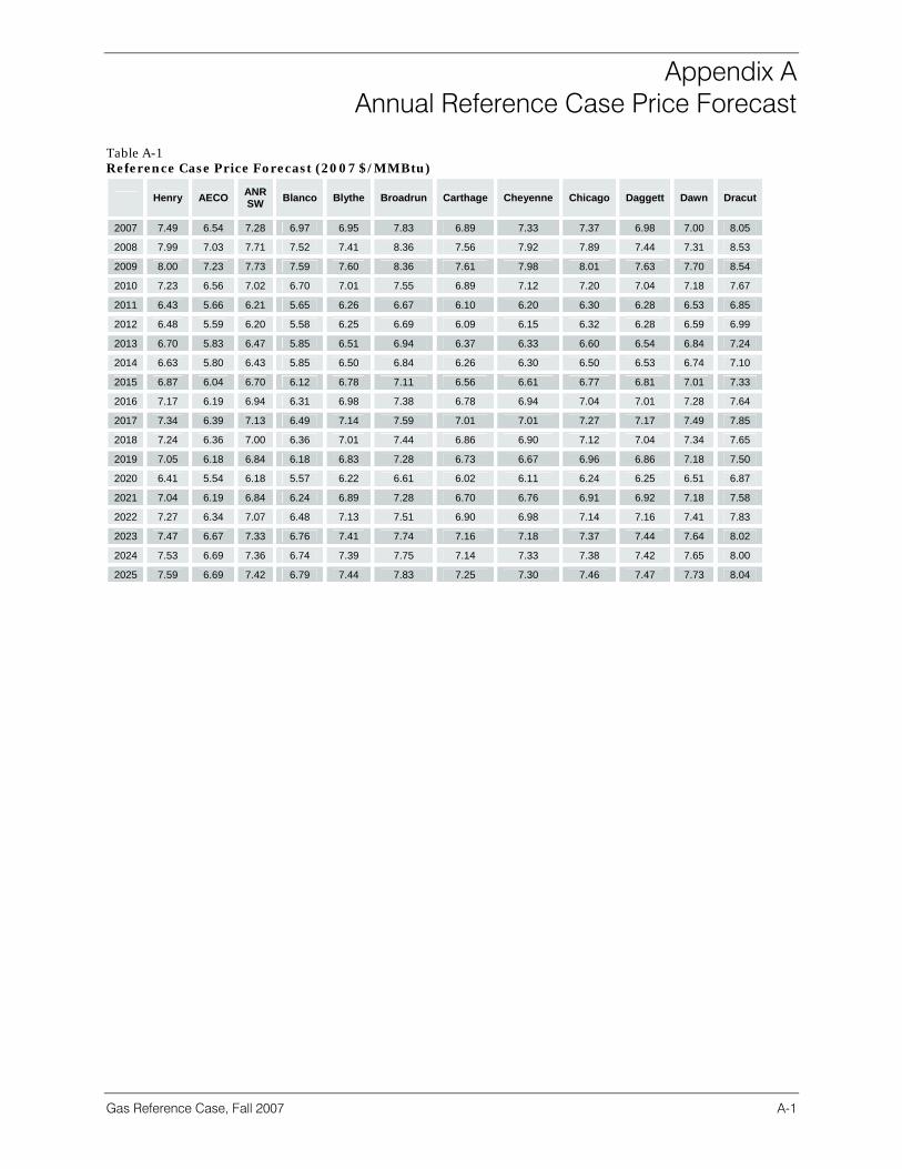
Appendix A Annual Reference Case Price Forecast
Gas Reference Case, Fall 2007 A-1
Table A-1 Reference Case Price Forecast (2007 $/MMBtu)
Henry AECO ANR SW Blanco Blythe Broadrun Carthage Cheyenne Chicago Daggett Dawn Dracut
2007 7.49 6.54 7.28 6.97 6.95 7.83 6.89 7.33 7.37 6.98 7.00 8.05
2008 7.99 7.03 7.71 7.52 7.41 8.36 7.56 7.92 7.89 7.44 7.31 8.53
2009 8.00 7.23 7.73 7.59 7.60 8.36 7.61 7.98 8.01 7.63 7.70 8.54
2010 7.23 6.56 7.02 6.70 7.01 7.55 6.89 7.12 7.20 7.04 7.18 7.67
2011 6.43 5.66 6.21 5.65 6.26 6.67 6.10 6.20 6.30 6.28 6.53 6.85
2012 6.48 5.59 6.20 5.58 6.25 6.69 6.09 6.15 6.32 6.28 6.59 6.99
2013 6.70 5.83 6.47 5.85 6.51 6.94 6.37 6.33 6.60 6.54 6.84 7.24
2014 6.63 5.80 6.43 5.85 6.50 6.84 6.26 6.30 6.50 6.53 6.74 7.10
2015 6.87 6.04 6.70 6.12 6.78 7.11 6.56 6.61 6.77 6.81 7.01 7.33
2016 7.17 6.19 6.94 6.31 6.98 7.38 6.78 6.94 7.04 7.01 7.28 7.64
2017 7.34 6.39 7.13 6.49 7.14 7.59 7.01 7.01 7.27 7.17 7.49 7.85
2018 7.24 6.36 7.00 6.36 7.01 7.44 6.86 6.90 7.12 7.04 7.34 7.65
2019 7.05 6.18 6.84 6.18 6.83 7.28 6.73 6.67 6.96 6.86 7.18 7.50
2020 6.41 5.54 6.18 5.57 6.22 6.61 6.02 6.11 6.24 6.25 6.51 6.87
2021 7.04 6.19 6.84 6.24 6.89 7.28 6.70 6.76 6.91 6.92 7.18 7.58
2022 7.27 6.34 7.07 6.48 7.13 7.51 6.90 6.98 7.14 7.16 7.41 7.83
2023 7.47 6.67 7.33 6.76 7.41 7.74 7.16 7.18 7.37 7.44 7.64 8.02
2024 7.53 6.69 7.36 6.74 7.39 7.75 7.14 7.33 7.38 7.42 7.65 8.00
2025 7.59 6.69 7.42 6.79 7.44 7.83 7.25 7.30 7.46 7.47 7.73 8.04
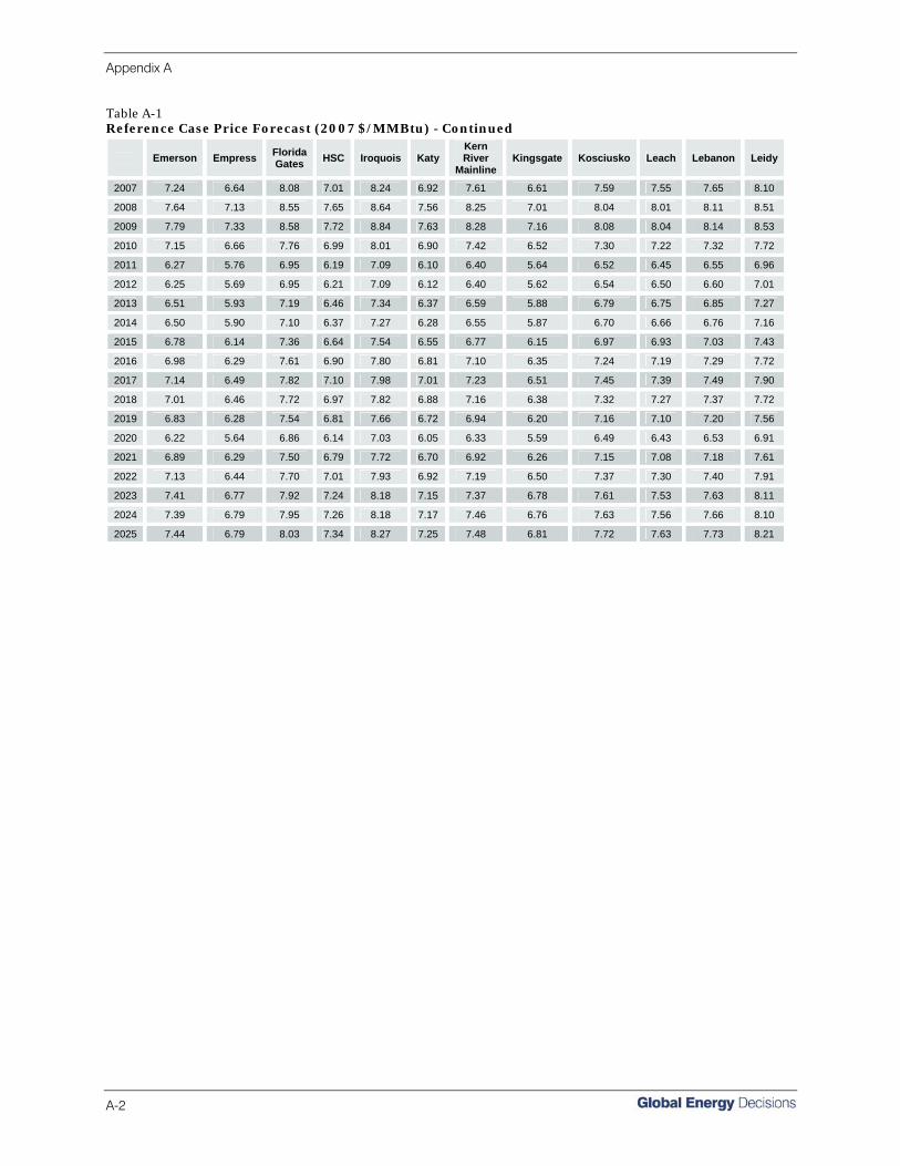
Appendix A
A-2
Table A-1 Reference Case Price Forecast (2007 $/MMBtu) - Continued
Emerson Empress Florida Gates HSC Iroquois Katy
Kern River
Mainline Kingsgate Kosciusko Leach Lebanon Leidy
2007 7.24 6.64 8.08 7.01 8.24 6.92 7.61 6.61 7.59 7.55 7.65 8.10
2008 7.64 7.13 8.55 7.65 8.64 7.56 8.25 7.01 8.04 8.01 8.11 8.51
2009 7.79 7.33 8.58 7.72 8.84 7.63 8.28 7.16 8.08 8.04 8.14 8.53
2010 7.15 6.66 7.76 6.99 8.01 6.90 7.42 6.52 7.30 7.22 7.32 7.72
2011 6.27 5.76 6.95 6.19 7.09 6.10 6.40 5.64 6.52 6.45 6.55 6.96
2012 6.25 5.69 6.95 6.21 7.09 6.12 6.40 5.62 6.54 6.50 6.60 7.01
2013 6.51 5.93 7.19 6.46 7.34 6.37 6.59 5.88 6.79 6.75 6.85 7.27
2014 6.50 5.90 7.10 6.37 7.27 6.28 6.55 5.87 6.70 6.66 6.76 7.16
2015 6.78 6.14 7.36 6.64 7.54 6.55 6.77 6.15 6.97 6.93 7.03 7.43
2016 6.98 6.29 7.61 6.90 7.80 6.81 7.10 6.35 7.24 7.19 7.29 7.72
2017 7.14 6.49 7.82 7.10 7.98 7.01 7.23 6.51 7.45 7.39 7.49 7.90
2018 7.01 6.46 7.72 6.97 7.82 6.88 7.16 6.38 7.32 7.27 7.37 7.72
2019 6.83 6.28 7.54 6.81 7.66 6.72 6.94 6.20 7.16 7.10 7.20 7.56
2020 6.22 5.64 6.86 6.14 7.03 6.05 6.33 5.59 6.49 6.43 6.53 6.91
2021 6.89 6.29 7.50 6.79 7.72 6.70 6.92 6.26 7.15 7.08 7.18 7.61
2022 7.13 6.44 7.70 7.01 7.93 6.92 7.19 6.50 7.37 7.30 7.40 7.91
2023 7.41 6.77 7.92 7.24 8.18 7.15 7.37 6.78 7.61 7.53 7.63 8.11
2024 7.39 6.79 7.95 7.26 8.18 7.17 7.46 6.76 7.63 7.56 7.66 8.10
2025 7.44 6.79 8.03 7.34 8.27 7.25 7.48 6.81 7.72 7.63 7.73 8.21
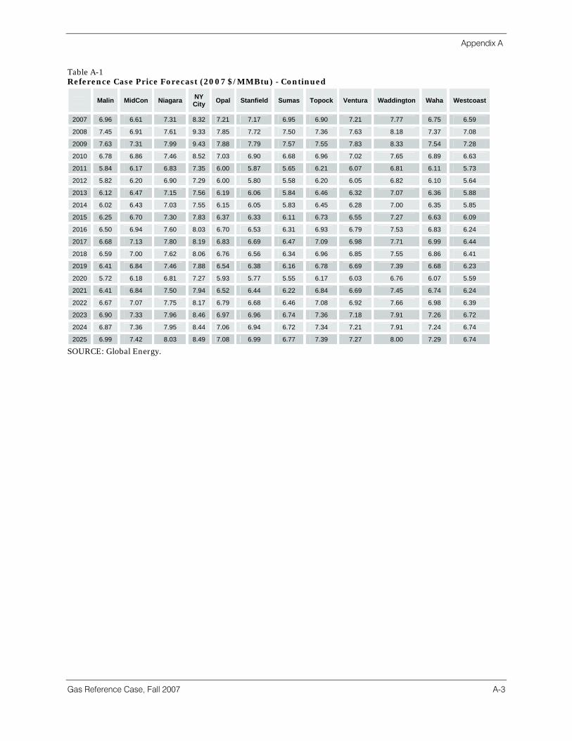
Appendix A
Gas Reference Case, Fall 2007 A-3
Table A-1 Reference Case Price Forecast (2007 $/MMBtu) - Continued
Malin MidCon Niagara NY City Opal Stanfield Sumas Topock Ventura Waddington Waha Westcoast
2007 6.96 6.61 7.31 8.32 7.21 7.17 6.95 6.90 7.21 7.77 6.75 6.59
2008 7.45 6.91 7.61 9.33 7.85 7.72 7.50 7.36 7.63 8.18 7.37 7.08
2009 7.63 7.31 7.99 9.43 7.88 7.79 7.57 7.55 7.83 8.33 7.54 7.28
2010 6.78 6.86 7.46 8.52 7.03 6.90 6.68 6.96 7.02 7.65 6.89 6.63
2011 5.84 6.17 6.83 7.35 6.00 5.87 5.65 6.21 6.07 6.81 6.11 5.73
2012 5.82 6.20 6.90 7.29 6.00 5.80 5.58 6.20 6.05 6.82 6.10 5.64
2013 6.12 6.47 7.15 7.56 6.19 6.06 5.84 6.46 6.32 7.07 6.36 5.88
2014 6.02 6.43 7.03 7.55 6.15 6.05 5.83 6.45 6.28 7.00 6.35 5.85
2015 6.25 6.70 7.30 7.83 6.37 6.33 6.11 6.73 6.55 7.27 6.63 6.09
2016 6.50 6.94 7.60 8.03 6.70 6.53 6.31 6.93 6.79 7.53 6.83 6.24
2017 6.68 7.13 7.80 8.19 6.83 6.69 6.47 7.09 6.98 7.71 6.99 6.44
2018 6.59 7.00 7.62 8.06 6.76 6.56 6.34 6.96 6.85 7.55 6.86 6.41
2019 6.41 6.84 7.46 7.88 6.54 6.38 6.16 6.78 6.69 7.39 6.68 6.23
2020 5.72 6.18 6.81 7.27 5.93 5.77 5.55 6.17 6.03 6.76 6.07 5.59
2021 6.41 6.84 7.50 7.94 6.52 6.44 6.22 6.84 6.69 7.45 6.74 6.24
2022 6.67 7.07 7.75 8.17 6.79 6.68 6.46 7.08 6.92 7.66 6.98 6.39
2023 6.90 7.33 7.96 8.46 6.97 6.96 6.74 7.36 7.18 7.91 7.26 6.72
2024 6.87 7.36 7.95 8.44 7.06 6.94 6.72 7.34 7.21 7.91 7.24 6.74
2025 6.99 7.42 8.03 8.49 7.08 6.99 6.77 7.39 7.27 8.00 7.29 6.74
SOURCE: Global Energy.

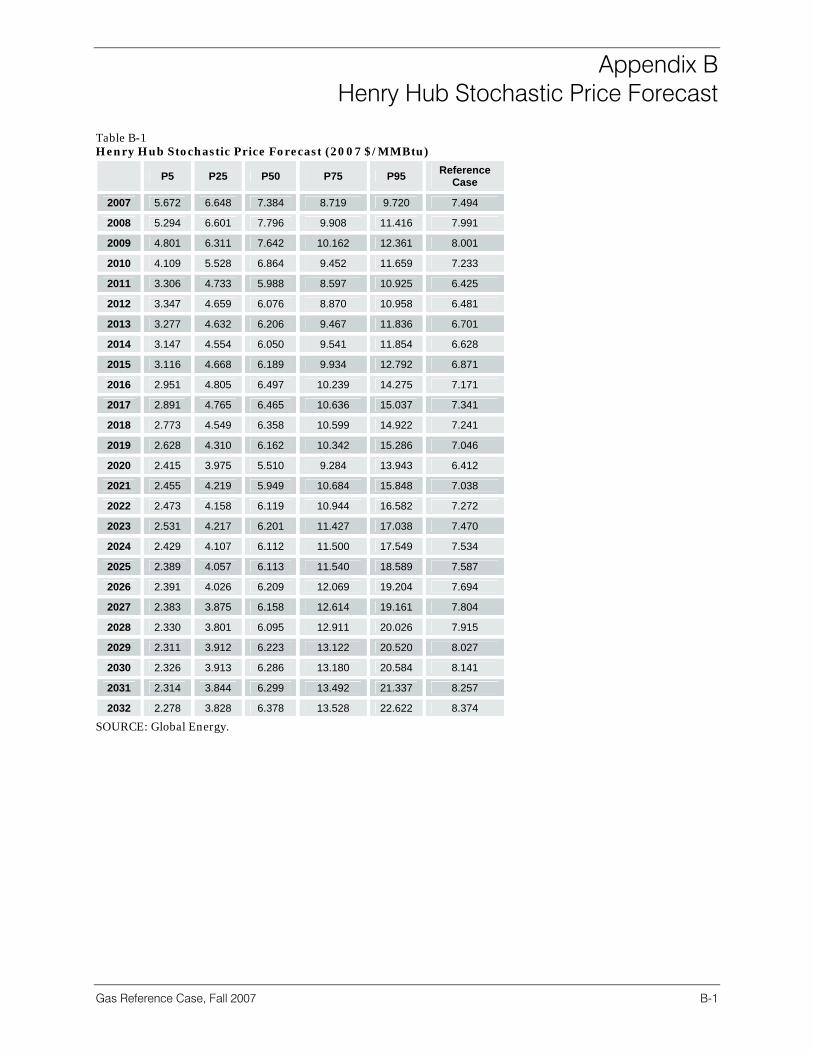
Appendix B Henry Hub Stochastic Price Forecast
Gas Reference Case, Fall 2007 B-1
Table B-1 Henry Hub Stochastic Price Forecast (2007 $/MMBtu)
P5 P25 P50 P75 P95 Reference Case
2007 5.672 6.648 7.384 8.719 9.720 7.494
2008 5.294 6.601 7.796 9.908 11.416 7.991
2009 4.801 6.311 7.642 10.162 12.361 8.001
2010 4.109 5.528 6.864 9.452 11.659 7.233
2011 3.306 4.733 5.988 8.597 10.925 6.425
2012 3.347 4.659 6.076 8.870 10.958 6.481
2013 3.277 4.632 6.206 9.467 11.836 6.701
2014 3.147 4.554 6.050 9.541 11.854 6.628
2015 3.116 4.668 6.189 9.934 12.792 6.871
2016 2.951 4.805 6.497 10.239 14.275 7.171
2017 2.891 4.765 6.465 10.636 15.037 7.341
2018 2.773 4.549 6.358 10.599 14.922 7.241
2019 2.628 4.310 6.162 10.342 15.286 7.046
2020 2.415 3.975 5.510 9.284 13.943 6.412
2021 2.455 4.219 5.949 10.684 15.848 7.038
2022 2.473 4.158 6.119 10.944 16.582 7.272
2023 2.531 4.217 6.201 11.427 17.038 7.470
2024 2.429 4.107 6.112 11.500 17.549 7.534
2025 2.389 4.057 6.113 11.540 18.589 7.587
2026 2.391 4.026 6.209 12.069 19.204 7.694
2027 2.383 3.875 6.158 12.614 19.161 7.804
2028 2.330 3.801 6.095 12.911 20.026 7.915
2029 2.311 3.912 6.223 13.122 20.520 8.027
2030 2.326 3.913 6.286 13.180 20.584 8.141
2031 2.314 3.844 6.299 13.492 21.337 8.257
2032 2.278 3.828 6.378 13.528 22.622 8.374
SOURCE: Global Energy.

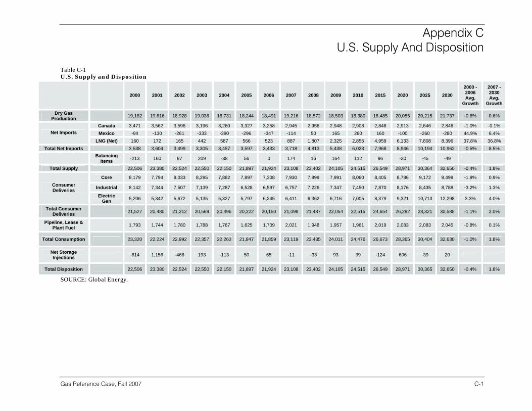
Appendix C U.S. Supply And Disposition
Gas Reference Case, Fall 2007 C-1
Table C-1 U.S. Supply and Disposition
2000 2001 2002 2003 2004 2005 2006 2007 2008 2009 2010 2015 2020 2025 2030 2000 - 2006 Avg.
Growth
2007 - 2030 Avg.
Growth
Dry Gas Production 19,182 19,616 18,928 19,036 18,731 18,244 18,491 19,216 18,572 18,503 18,380 18,485 20,055 20,215 21,737 -0.6% 0.6%
Canada 3,471 3,562 3,596 3,196 3,260 3,327 3,258 2,945 2,956 2,948 2,908 2,848 2,913 2,646 2,846 -1.0% -0.1% Mexico -94 -130 -261 -333 -390 -296 -347 -114 50 165 260 160 -100 -260 -280 44.9% 6.4% Net Imports
LNG (Net) 160 172 165 442 587 566 523 887 1,807 2,325 2,856 4,959 6,133 7,808 8,396 37.8% 36.8% Total Net Imports 3,538 3,604 3,499 3,305 3,457 3,597 3,433 3,718 4,813 5,438 6,023 7,968 8,946 10,194 10,962 -0.5% 8.5%
Balancing Items -213 160 97 209 -38 56 0 174 16 164 112 96 -30 -45 -49
Total Supply 22,506 23,380 22,524 22,550 22,150 21,897 21,924 23,108 23,402 24,105 24,515 26,549 28,971 30,364 32,650 -0.4% 1.8%
Core 8,179 7,794 8,033 8,295 7,882 7,897 7,308 7,930 7,899 7,991 8,060 8,405 8,786 9,172 9,499 -1.8% 0.9%
Industrial 8,142 7,344 7,507 7,139 7,287 6,528 6,597 6,757 7,226 7,347 7,450 7,870 8,176 8,435 8,788 -3.2% 1.3% Consumer Deliveries
Electric Gen 5,206 5,342 5,672 5,135 5,327 5,797 6,245 6,411 6,362 6,716 7,005 8,379 9,321 10,713 12,298 3.3% 4.0%
Total Consumer Deliveries 21,527 20,480 21,212 20,569 20,496 20,222 20,150 21,098 21,487 22,054 22,515 24,654 26,282 28,321 30,585 -1.1% 2.0%
Pipeline, Lease & Plant Fuel 1,793 1,744 1,780 1,788 1,767 1,625 1,709 2,021 1,948 1,957 1,961 2,019 2,083 2,083 2,045 -0.8% 0.1%
Total Consumption 23,320 22,224 22,992 22,357 22,263 21,847 21,859 23,119 23,435 24,011 24,476 26,673 28,365 30,404 32,630 -1.0% 1.8%
Net Storage Injections -814 1,156 -468 193 -113 50 65 -11 -33 93 39 -124 606 -39 20
Total Disposition 22,506 23,380 22,524 22,550 22,150 21,897 21,924 23,108 23,402 24,105 24,515 26,549 28,971 30,365 32,650 -0.4% 1.8%
SOURCE: Global Energy.


Appendix D Demand Forecast (MMcf/d)
Gas Reference Case, Fall 2007 D-1
Table D-1 Demand Forecast
2007 2008 2009 2010 2011 2012 2013 2014 2015 2016 2017 2018 2019 2020 2021 2022 2023 2024 2025 2026 2027 2028 2029 2030
ENC Residential 3,706 3,718 3,673 3,672 3,680 3,682 3,733 3,760 3,776 3,798 3,806 3,795 3,797 3,799 3,801 3,811 3,818 3,820 3,814 3,853 3,862 3,879 3,895 3,912
Commercial 1,900 1,920 1,939 1,959 1,978 1,998 2,019 2,041 2,063 2,084 2,106 2,128 2,150 2,171 2,194 2,217 2,240 2,263 2,277 2,299 2,308 2,326 2,342 2,358
Industrial 3,607 3,716 3,855 3,962 4,065 4,160 4,238 4,307 4,348 4,391 4,431 4,478 4,526 4,584 4,628 4,662 4,691 4,721 4,752 4,713 4,721 4,717 4,713 4,709
Electric Gen 602 661 711 756 661 717 783 847 895 918 939 1,006 1,013 977 1,050 1,077 1,105 1,133 1,160 1,188 1,216 1,244 1,271 1,299
ESC Residential 524 526 532 535 538 539 546 550 553 558 561 562 565 569 573 576 578 582 585 588 592 595 599 602
Commercial 399 404 408 413 418 423 428 433 438 444 449 455 460 466 472 478 484 490 496 499 504 508 513 518
Industrial 1,292 1,307 1,321 1,335 1,349 1,365 1,381 1,398 1,415 1,433 1,451 1,470 1,488 1,507 1,525 1,545 1,565 1,585 1,605 1,629 1,651 1,673 1,696 1,718
Electric Gen 613 705 789 837 885 949 1,028 1,146 1,225 1,297 1,399 1,468 1,474 1,477 1,546 1,632 1,718 1,803 1,889 1,975 2,061 2,146 2,232 2,318
MA Residential 2,368 2,350 2,412 2,415 2,399 2,372 2,385 2,383 2,387 2,406 2,415 2,410 2,425 2,437 2,445 2,447 2,452 2,463 2,472 2,488 2,500 2,512 2,525 2,537
Commercial 1,677 1,684 1,690 1,697 1,704 1,711 1,719 1,727 1,736 1,745 1,753 1,762 1,771 1,779 1,788 1,797 1,806 1,815 1,824 1,835 1,838 1,848 1,856 1,864
Industrial 883 892 901 910 919 928 938 947 957 966 976 986 995 1,005 1,015 1,026 1,036 1,046 1,057 1,072 1,085 1,098 1,111 1,124
Electric Gen 1,725 1,827 1,898 1,945 1,967 1,938 1,927 2,059 2,138 2,131 2,203 2,299 2,240 2,212 2,299 2,414 2,528 2,643 2,758 2,872 2,987 3,101 3,216 3,331
MNT Residential 886 899 919 934 949 962 976 989 1,003 1,018 1,032 1,048 1,065 1,080 1,098 1,118 1,136 1,154 1,172 1,162 1,171 1,174 1,178 1,182
Commercial 567 576 586 597 609 621 632 643 653 664 673 684 694 706 719 729 740 750 761 764 778 785 794 803
Industrial 708 715 723 731 740 747 755 763 770 777 785 792 800 808 816 823 830 838 845 856 865 874 884 893
Electric Gen 1,593 1,549 1,675 1,682 1,725 1,904 2,045 2,141 2,263 2,331 2,398 2,544 2,671 2,696 2,829 2,936 3,044 3,151 3,258 3,365 3,473 3,580 3,687 3,794
NE Residential 504 497 526 537 541 533 529 527 528 533 535 537 543 548 552 552 554 558 562 555 556 555 553 552
Commercial 329 333 336 339 342 345 349 354 359 364 369 374 379 384 389 395 400 406 412 420 422 429 434 440
Industrial 315 318 320 323 326 328 331 334 337 340 343 345 348 351 354 357 360 363 367 369 371 374 377 379
Electric Gen 1,243 1,323 1,359 1,376 1,370 1,341 1,391 1,532 1,600 1,581 1,648 1,725 1,723 1,722 1,738 1,796 1,853 1,910 1,967 2,024 2,082 2,139 2,196 2,253
PAC Residential 1,741 1,762 1,801 1,823 1,842 1,858 1,876 1,890 1,906 1,927 1,946 1,963 1,986 2,009 2,030 2,048 2,067 2,089 2,112 2,125 2,144 2,162 2,180 2,198
Commercial 905 915 928 941 953 964 973 985 996 1,007 1,019 1,032 1,044 1,057 1,069 1,082 1,095 1,108 1,122 1,120 1,138 1,143 1,152 1,161
Industrial 2,317 2,339 2,380 2,427 2,476 2,520 2,548 2,567 2,584 2,598 2,608 2,623 2,640 2,667 2,685 2,698 2,710 2,723 2,737 2,753 2,767 2,782 2,797 2,812
Electric Gen 3,011 2,931 2,981 3,125 3,135 3,352 3,425 3,567 3,702 3,812 3,834 3,983 4,106 4,198 4,305 4,399 4,495 4,591 4,686 4,782 4,878 4,973 5,069 5,165
SA Residential 1,194 1,209 1,228 1,244 1,260 1,275 1,292 1,308 1,324 1,342 1,358 1,373 1,390 1,408 1,425 1,442 1,459 1,477 1,494 1,505 1,520 1,534 1,548 1,562
Commercial 979 997 1,016 1,036 1,058 1,079 1,101 1,123 1,145 1,166 1,187 1,210 1,233 1,256 1,280 1,304 1,328 1,352 1,378 1,392 1,418 1,437 1,458 1,479
Industrial 1,319 1,334 1,359 1,385 1,413 1,437 1,456 1,472 1,486 1,498 1,509 1,522 1,536 1,553 1,566 1,576 1,584 1,593 1,604 1,609 1,618 1,626 1,634 1,643
Electric Gen 2,435 2,667 3,005 3,341 3,480 3,451 3,627 4,050 4,369 4,548 4,741 5,271 5,328 5,372 5,714 5,967 6,219 6,471 6,724 6,976 7,228 7,481 7,733 7,985
WNC Residential 1,229 1,231 1,227 1,227 1,228 1,229 1,241 1,249 1,257 1,266 1,273 1,276 1,282 1,287 1,292 1,299 1,306 1,312 1,317 1,328 1,335 1,343 1,351 1,359
Commercial 824 834 845 856 867 878 890 901 913 925 937 949 962 975 988 1,000 1,014 1,027 1,041 1,048 1,061 1,071 1,082 1,093
Industrial 1,320 1,371 1,425 1,461 1,496 1,530 1,569 1,607 1,631 1,656 1,680 1,703 1,728 1,755 1,782 1,810 1,839 1,868 1,898 1,926 1,955 1,985 2,014 2,043
Electric Gen 217 236 282 297 267 300 329 341 348 357 361 376 366 364 389 383 378 372 366 360 355 349 343 338
WSC Residential 930 943 970 985 998 1,008 1,020 1,030 1,041 1,054 1,065 1,076 1,090 1,103 1,116 1,126 1,137 1,149 1,161 1,165 1,175 1,183 1,191 1,199
Commercial 836 850 864 878 892 907 923 939 956 973 990 1,008 1,025 1,043 1,062 1,081 1,100 1,120 1,140 1,150 1,164 1,179 1,193 1,207
Industrial 7,766 7,805 7,844 7,878 7,911 7,944 7,978 8,011 8,040 8,069 8,098 8,127 8,157 8,186 8,216 8,246 8,276 8,306 8,337 8,462 8,523 8,601 8,679 8,756
Electric Gen 5,229 5,403 5,567 5,704 5,891 5,918 5,947 6,173 6,288 6,308 6,419 6,256 6,298 6,448 6,579 6,649 6,719 6,789 6,860 6,930 7,000 7,070 7,140 7,210
Table continued on next page.

Appendix D
D-2
US Residential 13,082 13,134 13,288 13,373 13,434 13,458 13,600 13,686 13,775 13,901 13,992 14,041 14,143 14,240 14,332 14,420 14,507 14,603 14,690 14,769 14,854 14,937 15,020 15,103
Commercial 8,416 8,512 8,612 8,715 8,820 8,927 9,035 9,147 9,258 9,371 9,484 9,601 9,717 9,837 9,959 10,083 10,207 10,332 10,450 10,527 10,631 10,728 10,825 10,923
Industrial 19,527 19,797 20,129 20,411 20,695 20,961 21,194 21,406 21,568 21,729 21,881 22,046 22,219 22,416 22,588 22,742 22,891 23,043 23,200 23,390 23,557 23,731 23,904 24,077
Electric Gen 16,668 17,301 18,267 19,063 19,382 19,870 20,502 21,857 22,827 23,281 23,942 24,928 25,220 25,466 26,449 27,254 28,059 28,864 29,669 30,473 31,278 32,083 32,888 33,693
CAN Residential 1,841 1,854 1,866 1,881 1,894 1,908 1,922 1,937 1,949 1,965 1,978 1,992 2,006 2,021 2,035 2,049 2,063 2,077 2,091 2,104 2,118 2,131 2,144 2,157
Commercial 1,542 1,550 1,560 1,584 1,600 1,618 1,636 1,651 1,669 1,691 1,712 1,739 1,775 1,802 1,816 1,828 1,841 1,854 1,866 1,896 1,915 1,934 1,959 1,981
Industrial 3,534 3,697 3,828 4,144 4,427 4,627 4,744 4,858 5,012 5,198 5,407 5,635 5,826 5,953 6,024 6,078 6,130 6,220 6,305 6,585 6,726 6,881 7,033 7,184
Electric Gen 830 893 909 944 906 990 1,124 1,167 1,219 1,258 1,294 1,344 1,319 1,365 1,412 1,459 1,507 1,555 1,603 1,651 1,699 1,746 1,794 1,842
SOURCE: Global Energy.

Appendix E Corridor Flow Forecast
Gas Reference Case, Fall 2007 E-1
Table E-1 Corridor Flow Forecast (MMcf/d) 2007
Source 2007 2010 2015 2020 2025
ENC AK-LA-TX Onshore 1,347 1,286 1,307 998 878
Alaska 513 931
Eastern US & Can. 279 173 258 197 163
GOM 819 852 857 507 215
LNG 560 1,127 1,782 1,416 1,867
Mackenzie 4 297 371
Midcontinent 2,140 2,063 2,123 1,608 1,583
North Central 645 318 289 229 244
Permian Basin 334 265 327 277 145
Rockies 1,607 2,256 2,430 2,925 2,811
WCSB 2,106 1,995 1,704 2,536 2,792
ESC AK-LA-TX Onshore 1,559 1,651 1,825 2,011 2,082
Eastern US & Can. 131 128 114 117 115
GOM 1,116 1,104 1,169 1,157 1,196
LNG 89 202 510 701 1,142
MA AK-LA-TX Onshore 1,745 1,337 1,111 1,033 1,046
Alaska 292 474
Eastern US & Can. 1,271 1,114 1,039 998 1,047
GOM 2,427 2,141 1,619 1,252 1,169
LNG 151 858 2,008 2,279 2,716
Mackenzie 1 101 130
Midcontinent 99 21 17 27 35
Rockies 75 323 325 384 482
WCSB 1,104 1,143 1,096 1,047 969
MNT LNG 2 234 294
Midcontinent 236 235 128 90 87
Permian Basin 135 172 198 106 112
Rockies 2,540 2,403 2,931 3,285 3,795
San Juan Basin 818 1,018 1,287 1,318 1,365
WCSB 129 118 147 150 188
NE AK-LA-TX Onshore 352 420 194 29 17
Eastern US & Can. 313 333 307 186 118
GOM 339 344 167 15 15
LNG 541 856 1,791 2,709 3,096
WCSB 696 557 353 40 36
PAC Alaska 735 1,076
California 749 697 676 602 584
LNG 495 1,215 1,804 2,471
Rockies 1,991 1,694 2,467 2,266 2,234
San Juan Basin 2,090 2,087 1,467 894 732
WCSB 2,792 3,068 3,101 3,113 2,971
SA AK-LA-TX Onshore 2,094 2,125 1,663 1,710 1,468
Table continued on next page.

Appendix E
E-2
Source 2007 2010 2015 2020 2025
Eastern US & Can. 509 436 481 564 580
GOM 2,517 1,989 1,661 2,010 1,830
LNG 864 2,296 4,424 5,010 6,596
Midcontinent 115 39 2 17 55
Rockies 13 99 95 189 322
WNC AK-LA-TX Onshore 221 242 342 227 221
Alaska 164 276
Midcontinent 1,925 2,120 2,154 2,022 1,921
Permian Basin 131 93 153 135 124
Rockies 936 918 1,209 1,262 1,422
WCSB 388 445 262 438 473
WSC AK-LA-TX Onshore 5,862 5,556 5,766 5,347 5,064
GOM 1,115 895 940 1,008 1,126
LNG 19 1,837 2,702 2,806 3,539
Midcontinent 3,150 3,177 3,199 3,527 3,707
Permian Basin 3,030 3,203 3,272 3,406 3,477
Rockies 436 383 345 359 349
San Juan Basin 363 180 112 294 243 SOURCE: Global Energy.
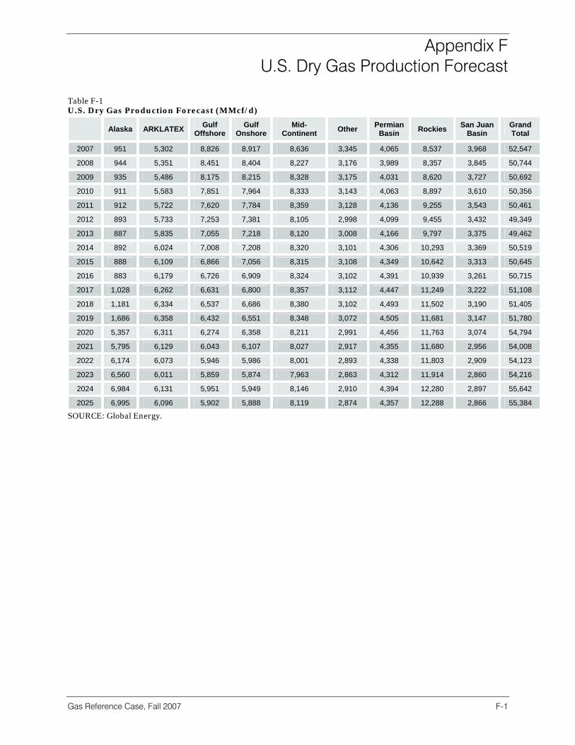
Appendix F U.S. Dry Gas Production Forecast
Gas Reference Case, Fall 2007 F-1
Table F-1 U.S. Dry Gas Production Forecast (MMcf/d)
Alaska ARKLATEX Gulf Offshore
Gulf Onshore
Mid-Continent Other Permian
Basin Rockies San Juan Basin
Grand Total
2007 951 5,302 8,826 8,917 8,636 3,345 4,065 8,537 3,968 52,547
2008 944 5,351 8,451 8,404 8,227 3,176 3,989 8,357 3,845 50,744
2009 935 5,486 8,175 8,215 8,328 3,175 4,031 8,620 3,727 50,692
2010 911 5,583 7,851 7,964 8,333 3,143 4,063 8,897 3,610 50,356
2011 912 5,722 7,620 7,784 8,359 3,128 4,136 9,255 3,543 50,461
2012 893 5,733 7,253 7,381 8,105 2,998 4,099 9,455 3,432 49,349
2013 887 5,835 7,055 7,218 8,120 3,008 4,166 9,797 3,375 49,462
2014 892 6,024 7,008 7,208 8,320 3,101 4,306 10,293 3,369 50,519
2015 888 6,109 6,866 7,056 8,315 3,108 4,349 10,642 3,313 50,645
2016 883 6,179 6,726 6,909 8,324 3,102 4,391 10,939 3,261 50,715
2017 1,028 6,262 6,631 6,800 8,357 3,112 4,447 11,249 3,222 51,108
2018 1,181 6,334 6,537 6,686 8,380 3,102 4,493 11,502 3,190 51,405
2019 1,686 6,358 6,432 6,551 8,348 3,072 4,505 11,681 3,147 51,780
2020 5,357 6,311 6,274 6,358 8,211 2,991 4,456 11,763 3,074 54,794
2021 5,795 6,129 6,043 6,107 8,027 2,917 4,355 11,680 2,956 54,008
2022 6,174 6,073 5,946 5,986 8,001 2,893 4,338 11,803 2,909 54,123
2023 6,560 6,011 5,859 5,874 7,963 2,863 4,312 11,914 2,860 54,216
2024 6,984 6,131 5,951 5,949 8,146 2,910 4,394 12,280 2,897 55,642
2025 6,995 6,096 5,902 5,888 8,119 2,874 4,357 12,288 2,866 55,384
SOURCE: Global Energy.

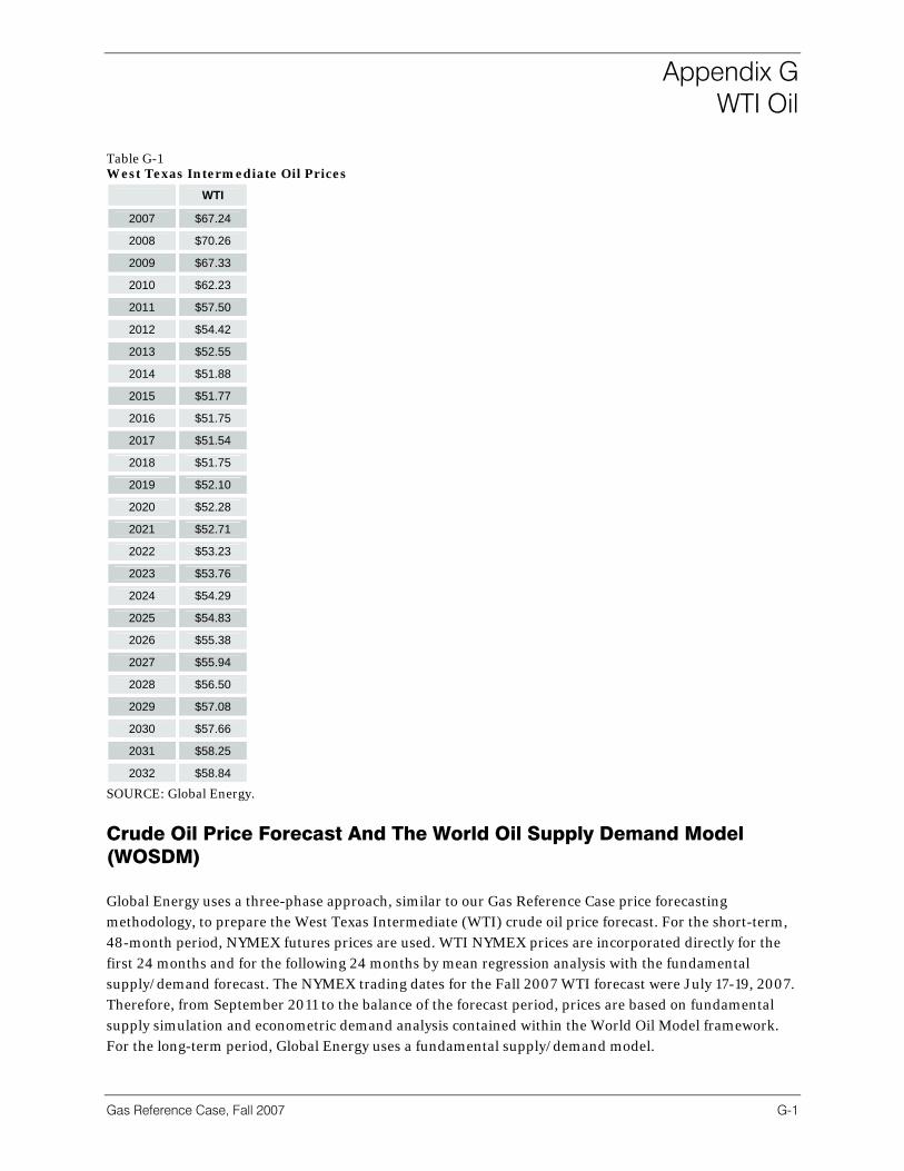
Appendix G WTI Oil
Gas Reference Case, Fall 2007 G-1
Table G-1 West Texas Intermediate Oil Prices
WTI
2007 $67.24
2008 $70.26
2009 $67.33
2010 $62.23
2011 $57.50
2012 $54.42
2013 $52.55
2014 $51.88
2015 $51.77
2016 $51.75
2017 $51.54
2018 $51.75
2019 $52.10
2020 $52.28
2021 $52.71
2022 $53.23
2023 $53.76
2024 $54.29
2025 $54.83
2026 $55.38
2027 $55.94
2028 $56.50
2029 $57.08
2030 $57.66
2031 $58.25
2032 $58.84
SOURCE: Global Energy.
Crude Oil Price Forecast And The World Oil Supply Demand Model (WOSDM) Global Energy uses a three-phase approach, similar to our Gas Reference Case price forecasting methodology, to prepare the West Texas Intermediate (WTI) crude oil price forecast. For the short-term, 48-month period, NYMEX futures prices are used. WTI NYMEX prices are incorporated directly for the first 24 months and for the following 24 months by mean regression analysis with the fundamental supply/demand forecast. The NYMEX trading dates for the Fall 2007 WTI forecast were July 17-19, 2007. Therefore, from September 2011 to the balance of the forecast period, prices are based on fundamental supply simulation and econometric demand analysis contained within the World Oil Model framework. For the long-term period, Global Energy uses a fundamental supply/demand model.

Appendix G
G-2
Global Energy’s World Oil Model (WOSDM) is a simulation forecasting model that tracks reserves, deliverability, and supply cost for 24 major oil producing countries and regions. The model considers the elements of oil supply cost such as exploration and development capital costs, royalties, operating costs by reserve category, and production taxes. The four reserve categories analyzed are Proved Developed, Proved Undeveloped, Unproved Probable, and Unproved Possible. Separate treatment of OPEC and non-OPEC producing countries is explicitly modeled to account for OPEC’s ability to withhold supply during periods of excess supply and to maintain solution prices above perfectly competitive levels. World demand is disaggregated into four geographic categories including: the United States, OECD without the United States, Emerging Market Countries, and the former Soviet Union. The demand component of the model consists of an econometric representation that considers oil prices, lagged oil demand, and per capita gross domestic product as explanatory variables. WOSDM also explicitly considers reserve appreciation, the impact of technological cost reduction over time, alternative macroeconomic growth rates, and the degree of excess productive capacity or supply cushion that exists at any one time. Also examined are field reserve appreciation, technological cost reduction over time, maintenance of minimum reserve to production levels, and new field development. Price shocks can also be examined using the model. Key model outputs include market clearing oil prices, production by region/country, reserves by category by region/country, supply cost, and excess productive capacity or supply cushion. Table G-2 shows the current OPEC supply quota as far as a) the relatively small surplus production capacity (the vast majority of which continues to be Saudi Arabia), and b) how amenable and often the Saudis are willing to prop up prices to achieve a perceived “floor” price despite their very low cost of production. In this situation, two production cuts were announced within three months. However, tensions in the Middle East (i.e., in November 2006, Iran testing long-range missiles that can reach Israel and taking 15 British sailors and marines hostage in late March 2007) have a greater impact than production cuts as witnessed by the continued price rise and volatility. More recently, there has been increased “saber-rattling” by various countries concerning Iran. This was expected to be followed by the Saudis increasing production to take advantage of prices above $75 per barrel, and indeed, at OPEC’s most recent meeting in September, production quotas were increased by 500,000 barrels per day. Non-OPEC production surplus continues to be tight and has a direct impact on market prices. Table G-2 Current OPEC Supply Quota
Nov. 1, 2006
Targeted Production Cut
Production December 2006Capacity*
Surplus 000s/day %
Algeria -59 1,370 1,430 60 4.2%
Indonesia -39 860 860 0 0.0%
Iran -176 3,700 3,750 50 1.3%
Kuwait -100 2,500 2,,600 100 3.8%
Libya -72 1,650 1,700 50 2.9%
Nigeria -100 2,300 2,300 0 0.0%
Qatar -35 815 850 35 4.1%
Saudi Arabia* ** -380 8,800 10,500-11,000 1,700-2,200 16.2%-20%
Table continued on next page.
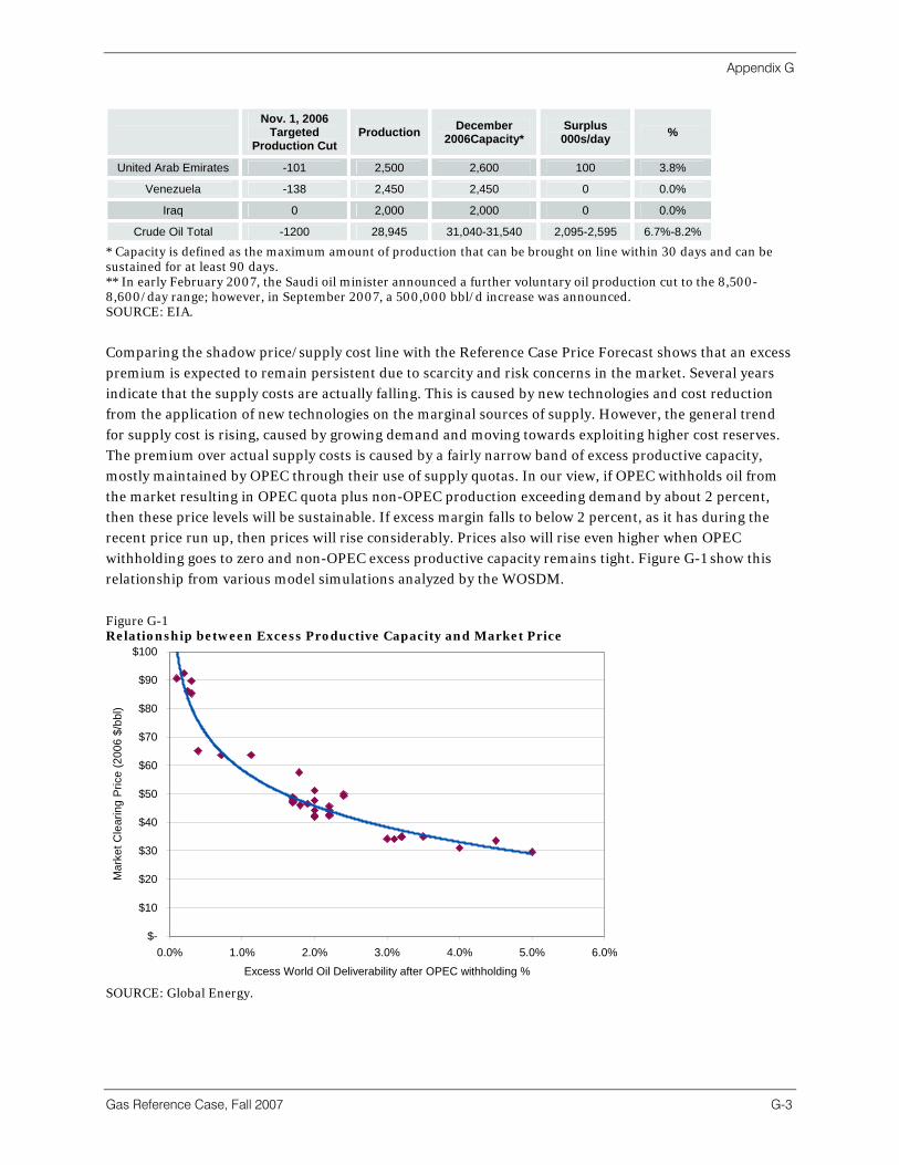
Appendix G
Gas Reference Case, Fall 2007 G-3
Nov. 1, 2006
Targeted Production Cut
Production December 2006Capacity*
Surplus 000s/day %
United Arab Emirates -101 2,500 2,600 100 3.8%
Venezuela -138 2,450 2,450 0 0.0%
Iraq 0 2,000 2,000 0 0.0%
Crude Oil Total -1200 28,945 31,040-31,540 2,095-2,595 6.7%-8.2%
* Capacity is defined as the maximum amount of production that can be brought on line within 30 days and can be sustained for at least 90 days. ** In early February 2007, the Saudi oil minister announced a further voluntary oil production cut to the 8,500-8,600/day range; however, in September 2007, a 500,000 bbl/d increase was announced. SOURCE: EIA.
Comparing the shadow price/supply cost line with the Reference Case Price Forecast shows that an excess premium is expected to remain persistent due to scarcity and risk concerns in the market. Several years indicate that the supply costs are actually falling. This is caused by new technologies and cost reduction from the application of new technologies on the marginal sources of supply. However, the general trend for supply cost is rising, caused by growing demand and moving towards exploiting higher cost reserves. The premium over actual supply costs is caused by a fairly narrow band of excess productive capacity, mostly maintained by OPEC through their use of supply quotas. In our view, if OPEC withholds oil from the market resulting in OPEC quota plus non-OPEC production exceeding demand by about 2 percent, then these price levels will be sustainable. If excess margin falls to below 2 percent, as it has during the recent price run up, then prices will rise considerably. Prices also will rise even higher when OPEC withholding goes to zero and non-OPEC excess productive capacity remains tight. Figure G-1 show this relationship from various model simulations analyzed by the WOSDM.
Figure G-1 Relationship between Excess Productive Capacity and Market Price
$-
$10
$20
$30
$40
$50
$60
$70
$80
$90
$100
0.0% 1.0% 2.0% 3.0% 4.0% 5.0% 6.0%
Excess World Oil Deliverability after OPEC withholding %
Mar
ket C
lear
ing
Pric
e (2
006
$/bb
l)
SOURCE: Global Energy.
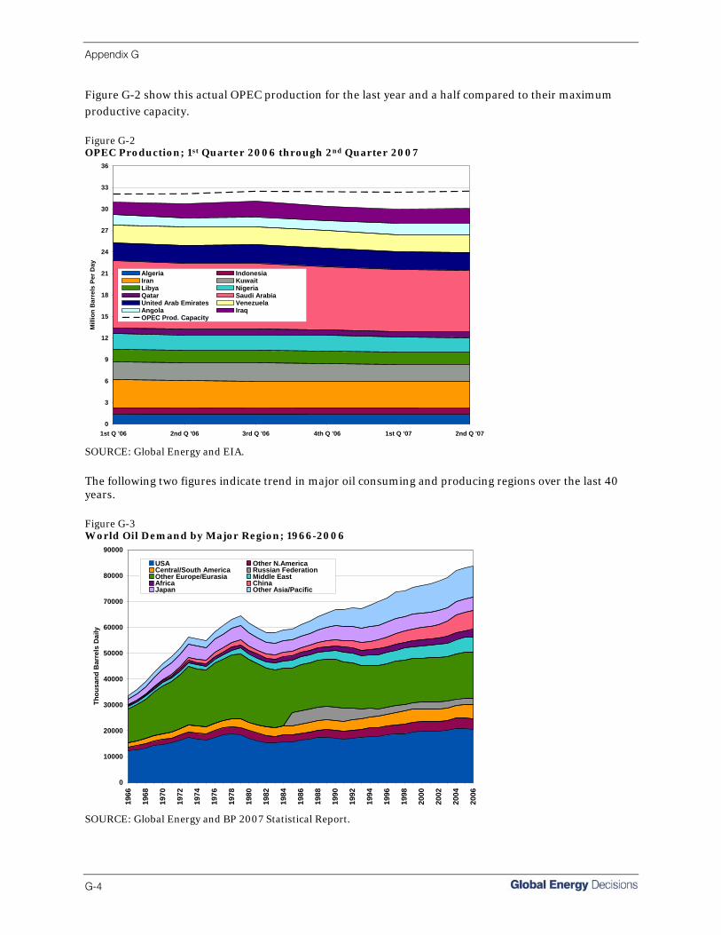
Appendix G
G-4
Figure G-2 show this actual OPEC production for the last year and a half compared to their maximum productive capacity. Figure G-2 OPEC Production; 1st Quarter 2006 through 2nd Quarter 2007
0
3
6
9
12
15
18
21
24
27
30
33
36
1st Q '06 2nd Q '06 3rd Q '06 4th Q '06 1st Q '07 2nd Q '07
Mill
ion
Bar
rels
Per
Day
Algeria IndonesiaIran KuwaitLibya NigeriaQatar Saudi ArabiaUnited Arab Emirates VenezuelaAngola IraqOPEC Prod. Capacity
SOURCE: Global Energy and EIA.
The following two figures indicate trend in major oil consuming and producing regions over the last 40 years. Figure G-3 World Oil Demand by Major Region; 1966-2006
0
10000
20000
30000
40000
50000
60000
70000
80000
90000
1966
1968
1970
1972
1974
1976
1978
1980
1982
1984
1986
1988
1990
1992
1994
1996
1998
2000
2002
2004
2006
Thou
sand
Bar
rels
Dai
ly
USA Other N.AmericaCentral/South America Russian FederationOther Europe/Eurasia Middle EastAfrica ChinaJapan Other Asia/Pacific
SOURCE: Global Energy and BP 2007 Statistical Report.
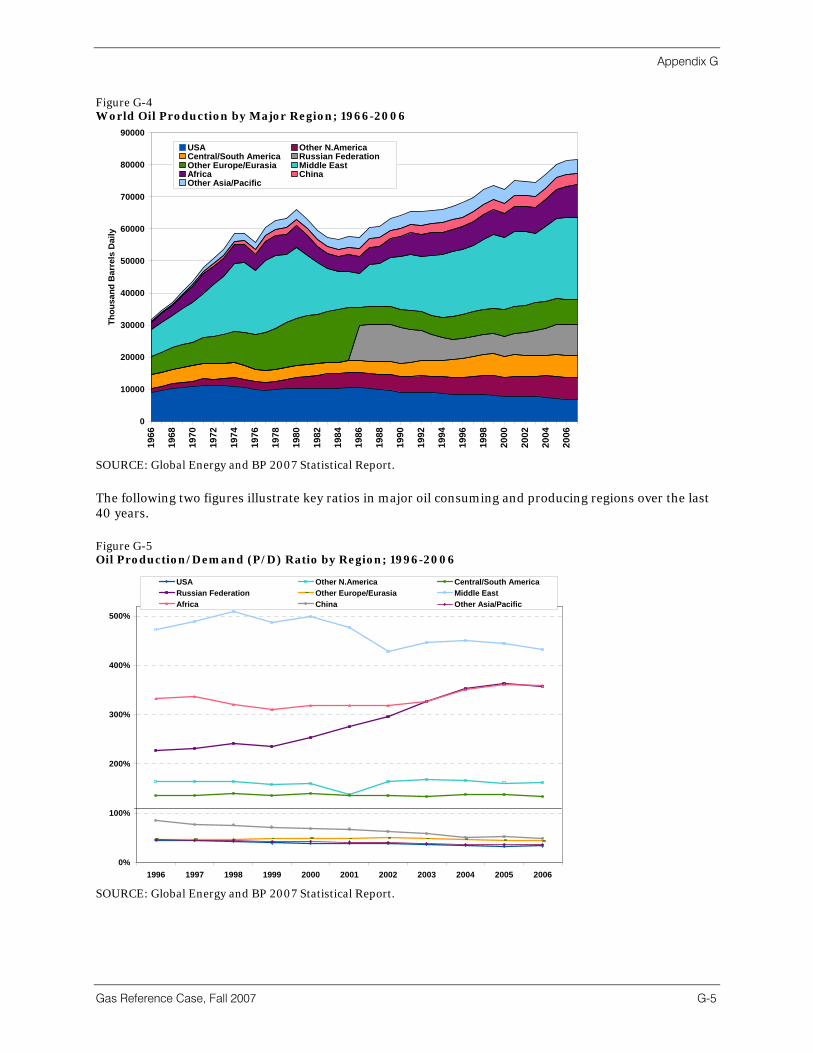
Appendix G
Gas Reference Case, Fall 2007 G-5
Figure G-4 World Oil Production by Major Region; 1966-2006
0
10000
20000
30000
40000
50000
60000
70000
80000
90000
1966
1968
1970
1972
1974
1976
1978
1980
1982
1984
1986
1988
1990
1992
1994
1996
1998
2000
2002
2004
2006
Thou
sand
Bar
rels
Dai
ly
USA Other N.AmericaCentral/South America Russian FederationOther Europe/Eurasia Middle EastAfrica ChinaOther Asia/Pacific
SOURCE: Global Energy and BP 2007 Statistical Report.
The following two figures illustrate key ratios in major oil consuming and producing regions over the last 40 years. Figure G-5 Oil Production/Demand (P/D) Ratio by Region; 1996-2006
0%
100%
200%
300%
400%
500%
1996 1997 1998 1999 2000 2001 2002 2003 2004 2005 2006
USA Other N.America Central/South AmericaRussian Federation Other Europe/Eurasia Middle EastAfrica China Other Asia/Pacific
SOURCE: Global Energy and BP 2007 Statistical Report.
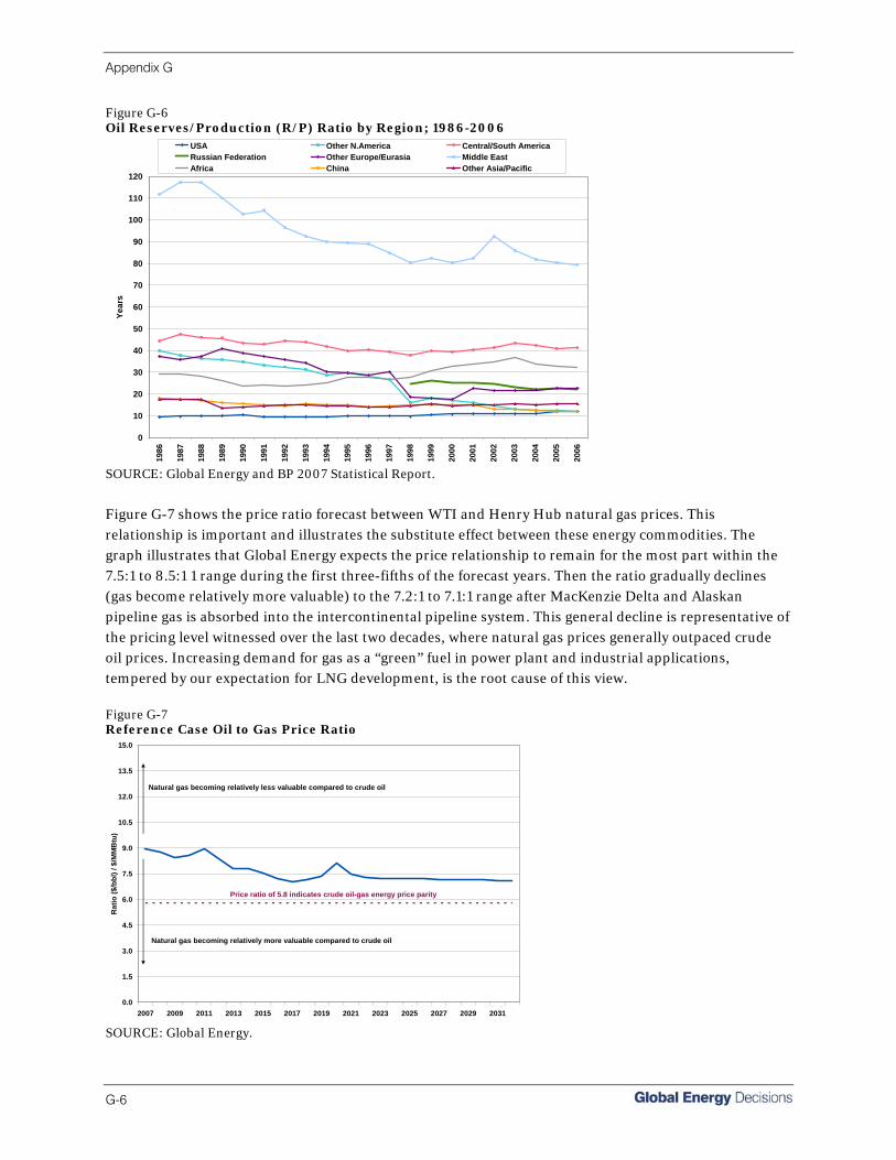
Appendix G
G-6
Figure G-6 Oil Reserves/Production (R/P) Ratio by Region; 1986-2006
0
10
20
30
40
50
60
70
80
90
100
110
120
1986
1987
1988
1989
1990
1991
1992
1993
1994
1995
1996
1997
1998
1999
2000
2001
2002
2003
2004
2005
2006
Year
s
USA Other N.America Central/South AmericaRussian Federation Other Europe/Eurasia Middle EastAfrica China Other Asia/Pacific
SOURCE: Global Energy and BP 2007 Statistical Report.
Figure G-7 shows the price ratio forecast between WTI and Henry Hub natural gas prices. This relationship is important and illustrates the substitute effect between these energy commodities. The graph illustrates that Global Energy expects the price relationship to remain for the most part within the 7.5:1 to 8.5:1 1 range during the first three-fifths of the forecast years. Then the ratio gradually declines (gas become relatively more valuable) to the 7.2:1 to 7.1:1 range after MacKenzie Delta and Alaskan pipeline gas is absorbed into the intercontinental pipeline system. This general decline is representative of the pricing level witnessed over the last two decades, where natural gas prices generally outpaced crude oil prices. Increasing demand for gas as a “green” fuel in power plant and industrial applications, tempered by our expectation for LNG development, is the root cause of this view. Figure G-7 Reference Case Oil to Gas Price Ratio
0.0
1.5
3.0
4.5
6.0
7.5
9.0
10.5
12.0
13.5
15.0
2007 2009 2011 2013 2015 2017 2019 2021 2023 2025 2027 2029 2031
Rat
io ($
/bbl
) / $
/MM
Btu
)
Natural gas becoming relatively more valuable compared to crude oil
Natural gas becoming relatively less valuable compared to crude oil
Price ratio of 5.8 indicates crude oil-gas energy price parity
SOURCE: Global Energy.
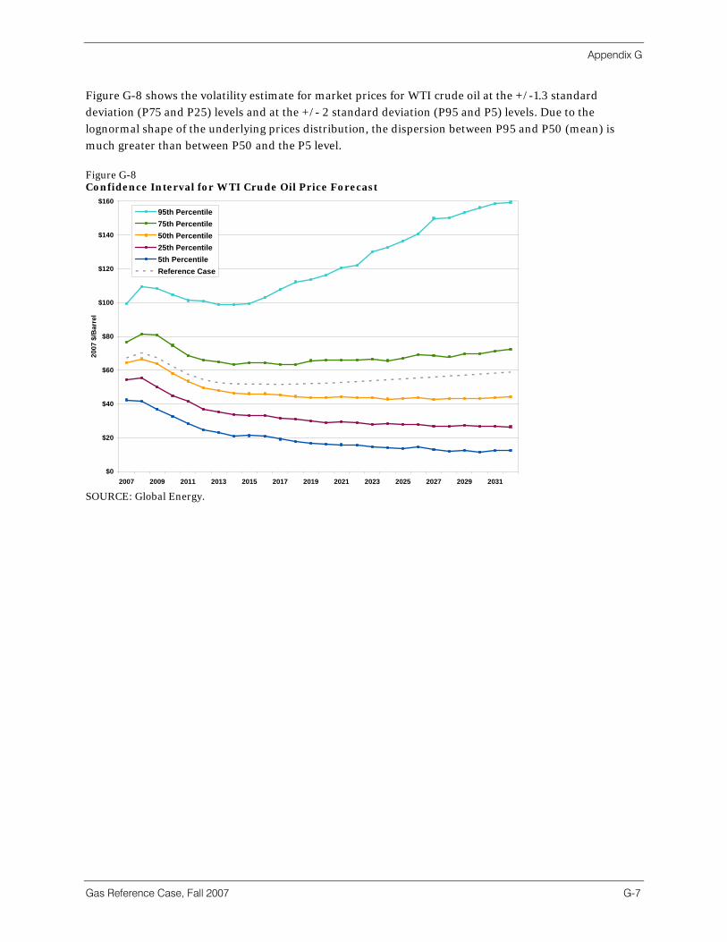
Appendix G
Gas Reference Case, Fall 2007 G-7
Figure G-8 shows the volatility estimate for market prices for WTI crude oil at the +/-1.3 standard deviation (P75 and P25) levels and at the +/- 2 standard deviation (P95 and P5) levels. Due to the lognormal shape of the underlying prices distribution, the dispersion between P95 and P50 (mean) is much greater than between P50 and the P5 level. Figure G-8 Confidence Interval for WTI Crude Oil Price Forecast
$0
$20
$40
$60
$80
$100
$120
$140
$160
2007 2009 2011 2013 2015 2017 2019 2021 2023 2025 2027 2029 2031
2007
$/B
arre
l
95th Percentile75th Percentile50th Percentile25th Percentile5th PercentileReference Case
SOURCE: Global Energy.

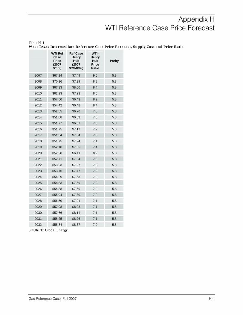
Appendix H WTI Reference Case Price Forecast
Gas Reference Case, Fall 2007 H-1
Table H-1 West Texas Intermediate Reference Case Price Forecast, Supply Cost and Price Ratio
WTI Ref Case Price (2007 $/bbl)
Ref Case Henry Hub
(2007 $/MMBtu)
WTI-Henry Hub Price Ratio
Parity
2007 $67.24 $7.49 9.0 5.8
2008 $70.26 $7.99 8.8 5.8
2009 $67.33 $8.00 8.4 5.8
2010 $62.23 $7.23 8.6 5.8
2011 $57.50 $6.43 8.9 5.8
2012 $54.42 $6.48 8.4 5.8
2013 $52.55 $6.70 7.8 5.8
2014 $51.88 $6.63 7.8 5.8
2015 $51.77 $6.87 7.5 5.8
2016 $51.75 $7.17 7.2 5.8
2017 $51.54 $7.34 7.0 5.8
2018 $51.75 $7.24 7.1 5.8
2019 $52.10 $7.05 7.4 5.8
2020 $52.28 $6.41 8.2 5.8
2021 $52.71 $7.04 7.5 5.8
2022 $53.23 $7.27 7.3 5.8
2023 $53.76 $7.47 7.2 5.8
2024 $54.29 $7.53 7.2 5.8
2025 $54.83 $7.59 7.2 5.8
2026 $55.38 $7.69 7.2 5.8
2027 $55.94 $7.80 7.2 5.8
2028 $56.50 $7.91 7.1 5.8
2029 $57.08 $8.03 7.1 5.8
2030 $57.66 $8.14 7.1 5.8
2031 $58.25 $8.26 7.1 5.8
2032 $58.84 $8.37 7.0 5.8
SOURCE: Global Energy.

Appendix I History And Evolution Of Natural Gas Deregulation
Gas Reference Case, Fall 2007 I-1
Natural gas has been regulated in the United States since the first small local distribution systems were created in the early to mid-1800s. Local governments, seeing the “natural monopoly” characteristics of the natural gas market and the usefulness of the product, decided that the natural gas distribution business affected the public interest to a sufficient extent to require regulation. Because of the distribution network that was needed to deliver natural gas to customers, it was decided that one company with a single distribution network could deliver natural gas more economically than two or three companies with overlying distribution networks and markets. This was patterned after the other primary regulated business at the time: bridge construction. However, economic theory dictates that a company in a monopoly position, with total control over its market and the absence of any competition will typically take advantage of its position, and has the incentive to charge overly high prices. The solution, from the point of view of the local governments, was to regulate the rates these natural monopolies charged and set down regulations that prevented them from abusing their market power, in effect acting as a substitute for competition.
As the natural gas industry further developed, so did the complexity of maintaining regulation. In the early 1900s, natural gas began to be shipped between municipalities, thus gas markets were no longer segmented by municipal boundaries. The first intrastate pipelines began carrying gas from city to city, and this new mobility of natural gas meant that local governments could no longer oversee the entire natural gas distribution chain. There was, in essence, a regulatory gap between municipalities. In response to this, state level governments intervened to regulate the new “intrastate” natural gas market and determined rates that could be charged by gas distributors. This was done by creating public utility commissions and public service commissions to oversee the regulation of natural gas distribution. The first states to do so were New York and Wisconsin, which instituted commissions as early as 1907. The federal government finally became involved when Congress passed the Federal Water Power Act in 1920 establishing the Federal Power Commission (FPC) to license hydroelectric projects by private companies and state and local government, and to handle natural gas regulations as well. Technical advances in pipeline construction in the early 1920s created a tremendous growth opportunity for the natural gas industry. Most states that had natural gas reserves became concerned about depleting their natural resources and losing tax revenue when gas was transported out of state. Consuming states and their constituents were concerned that they were paying unrealistically high prices for the gas they depended upon for their needs. And gas producers were worried that they were being paid less than market prices for their product but were powerless to intervene. A series of industry-related lawsuits came before the U.S. Supreme Court in the mid to late-1920s addressing these issues. States involved in these lawsuits sought the authority to regulate the commercial activities of pipelines within their own borders. The Court ruled that states did not have this authority to regulate the interstate purchase, sale, or transportation of natural gas. Furthermore, any attempt to do so would wrongfully interfere with interstate commerce. It should also be noted that an extensive interstate pipeline system did not really exist until after World War II. Most gas distribution systems, such as the one started in Boston in 1822, were supplied with manufactured carbureted coal gas (also known as water gas or manufactured gas) that was made by passing steam over hot soft coal. The coal tar residue from this low-Btu synthetic gas process even today is an environmental hazard in areas where it hasn’t been remedied.
Appendix I
I-2
Congress enacted the Public Utility Holding Company Act (PUHCA) in 1935 that prevents utility holding companies from subsidizing unregulated businesses with profits obtained from their regulated businesses and captive customers. All side businesses must be kept separate from their regulated businesses to prevent hiding inflated charges in their regulated rates (i.e., losses moved to regulated businesses and profits moved to deregulated businesses). The Act vested in the SEC extensive jurisdiction over electric and gas distribution holding companies. Interstate transmission pipelines were not subject to the Act. (The newly released FERC Order 2004 might be considered an evolution of the PUHCA from the prevention of the movement of “money” from regulated energy businesses to deregulated businesses to the prevention of the movement of “knowledge” or insider information from regulated energy businesses to deregulated businesses.) Finally, in 1938, the U.S. Congress acted. Regulatory control over the interstate sale and transportation of natural gas in the United States began with the Natural Gas Act (NGA) of 1938. Under the NGA, the FPC, the predecessor agency to the Federal Energy Regulatory Commission, was given three major powers: 1. The power to issue certificates of public convenience and necessity authorizing construction and
operation of physical facilities; 2. The power to regulate rates for sales for resale of natural gas in interstate commerce (gas which
crosses a state line) for public consumption; and 3. The power to regulate the transportation of gas in interstate commerce. A regulated commodity pricing and transportation rate structure quickly displaced the pipeline’s control over setting its own prices and rates. Along with this rate stability came an increased awareness that natural gas could be a reliable source of fuel. The NGA does not apply to other sales or transportation, to the local distribution of natural gas, to distribution facilities, or to the production and gathering of natural gas. The NGA exempts from FERC jurisdiction a pipeline that transports gas, or sale for resale gas, in interstate commerce if all the natural gas so received is ultimately consumed within one state. Known as a Hinshaw pipeline, it is essentially a pipeline with both supply and sales within one state but, for some geographic reason, crosses (and re-crosses) a state boundary. Of course, the pipeline by default is then state regulated. The U.S. interstate pipeline system received its biggest push thanks to the start of WWII in December 1941. In order to avoid the sinking of crude oil and refined oil product tankers by German U-boats attempting to cut off the East Coast from fuel supplies, a crash program by the War Production Board approved the building of the minimally coated steel “Big-Inch and Little Big-Inch” pipelines in early 1942. In one year construction was completed of the 1,254-mile long 24"- and 20"-diameter oil pipelines from the Texas and Louisiana oil fields northeasterly to industrial markets in Arkansas, Illinois, Indiana, Ohio, Pennsylvania, and up to New York City. These large diameter pipelines were a technological innovation at the time, about twice the diameter of existing gas pipelines and thus able to carry four times the volume. The 20"-diameter line was designed to handle as many as four different refined products, including gasoline, heating oil, diesel oil, and kerosene, each kept separate within the line by solid rubber balls. In
Appendix I
Gas Reference Case, Fall 2007 I-3
1946, the lines were auctioned off by the War Emergency Pipeline Corporation for $143 million and converted to transport natural gas. They became the backbone of the Texas Eastern Transmission System and served as a design template for long-line interstate pipeline competitors such as Transcontinental Gas Pipeline and Tennessee Gas Pipeline running from the Gulf Coast to the Northeast. In 1947, Subsection 7(h) was added to the NGA, which allowed pipeline certificate holders to acquire rights-of-way for a proposed pipeline, by eminent domain proceeding in the appropriate U.S. District Court. This proved to be a very powerful tool aiding the expansion of the U.S. pipeline system to serve “an expanding population with an expanding industrial or household use of gas.” By proclaiming a “right of eminent domain” to establish efficient transmission of gas, pipeline companies established a privileged “right of way” status that superseded the rights of individual property owners along the pipeline’s path to market. Concurrently, local and state agencies sought to regulate the pipelines with a myriad of parochial and arcane rules that sought to preserve their jurisdictional control over a growing industry that required a national perspective. In 1954, the FPC jurisdiction extended to the gas producer level as a result of the Phillips Petroleum Company v. FPC Supreme Court Case. Much of the interstate pipeline system was built during the 1950s and 1960s as local distribution companies connected to natural gas pipelines and stopped manufacturing their labor-intensive carbureted water gas. Since natural gas was relatively inexpensive to find, as well as being found along with oil deposits (associated gas), the regulatory system worked until exploration and production costs dramatically increased in the 1960s and 1970s, causing spot shortages in the mid-1970s. Market aberrations also occurred, such as large differences between intrastate and interstate gas prices. Producers would sell gas first to the unregulated intrastate markets, which had no price caps, serving interstate pipelines last. Consumers in producing states had a distinct advantage in obtaining adequate supplies of gas. Interstate pipelines would enter into take-or-pay contracts with producers at high percentage takes, in the 90 percent to 100 percent range, in order to secure long-term supplies. The year 1972 was the high point in utility gas sales as well as a peak in marketed consumption of about 22 Tcf. The period from 1972 to 1980 is generally regarded as one with a shortage of gas deliverability. In the midst of this shortage, at nearly the peak of the energy crises in 1977, the FPC was abolished and the Federal Energy Regulatory Commission (FERC) was created by the Department of Energy Organization Act. As the gas shortage and high prices continued, the Power Plant and Industrial Fuel Use Act was enacted in November 1978, limiting the use of natural gas in power plant and industrial boilers. The act was designed to require the conversion of electric generating plants and industrial boilers from oil or gas to coal or from gas to oil. No new power plants could be built that used natural gas or oil. Fortunately, the natural gas shortage was almost over by time this legislation passed, and due to the high costs of imported oil, the Secretary of Energy was encouraging large fuel users to switch from oil back to gas. Until the Act was repealed in 1987, however, any plant that wanted to increase its gas usage—or convert to dual-fuel usage—needed an exemption from the Fuel Use Act, easily granted. There was much confusion during this time period since the regulation was still on the books (requiring a phase-out of natural gas as a power plant fuel by 1990) while gas prices were dropping, a supply bubble was expanding, oil prices were rising, and government officials were promoting gas usage. Forty years after the passage of the NGA, a federal statute enacted in 1978 began to phase out producer rate regulation by January 1, 1985, setting escalating price ceilings on different vintages and types of
Appendix I
I-4
natural gas. Known as “Sections,” these ceiling prices and escalation factors depended upon the date of gas discovery, the drilling depth, and the geological formation from which it was found (e.g., tight sands, Devonian shale, Carboniferous, Permian, Triassic, Jurassic, etc.). Some gas sections were capped as low as $0.50/MMBtu while other sections (such as section 107) could exceed $7.00/MMBtu (in order to encourage further exploration of incremental supplies). Part of the problem with “vintaging” gas was that interstates would blend the gases together in order to obtain a weighted-average-cost-of-gas (WACOG) which tended to insulate all classes of consumers from what the incremental cost of actually finding and producing the next block of gas supply. Price signals were becoming very important to FERC. The Natural Gas Policy Act of 1978 (NGPA) provided these maximum lawful prices, including escalators (and no de-escalators) in over a dozen categories of gas subject to their price regulation. There was a general fear that on January 1, 1985 there would be a price “fly-up” when price caps were removed. The NGPA also provided for self-implementing transportation services (contained in Section 311), without the need for prior certificates of public convenience and necessity from FERC, for certain qualifying transportation by interstate or intrastate pipelines in certain instances. FERC Order 380 issued in the early 1980s required gas suppliers to recast contracts to allow buyers to be able to eliminate commodity purchases and eliminate minimum commodity bills. This was performed by designing two-part rates, where a demand charge covered all of a pipeline supplier’s fixed costs and a commodity charge would cover all of a pipeline supplier’s variable costs. With this Order, pipelines should be indifferent as to an LDC’s (Local Gas Distribution Company) level of gas takes since the pipeline would be theoretically receiving their allowed ROE without selling any gas. The result of the NGPA and Order 380 was that in early 1985, a gas price collapse (or “fly-down”) occurred due to the over-supply situation caused by over-drilling, leading to what is commonly referred to as the beginnings of the “gas bubble” (Additionally, gas deregulation was implemented in Canada. The Canadian Halloween Agreement passed in October 1985 allowed gas customers in eastern Canada to purchase gas supplies directly rather than from TransCanada PipeLines (TCPL). Purchasers of Canadian gas in the U.S. Midwest and Northeast benefited as well from the pent up Canadian supply now unencumbered by a requirement that suppliers have a 21-year reserve life in order to sell to TCPL. Crude oil price declines during this period also contributed to the “bubble” or “gas sausage”) which lasted for well over a decade and was characterized by low gas prices with occasional price “busts” or price collapse below the cost of production. Since that time, gas prices have followed generally a boom and bust price path until the late 1990s when prices have generally increased with occasional price “booms” to very high levels. To help deal with the serious gas surplus that began in the early 1980s, in 1983 FERC authorized temporary design of Special Marketing Programs (SMP) to regain lost pipeline customers by allowing third-party gas to replace up to 10 percent of an LDC’s maximum daily quantity traditionally bought from interstate pipelines. This was the first taste that LDCs had in the 160-year history of the U.S. gas business (the streets of Boston were first lit with gas in 1822) of purchasing natural gas directly from a producer, nominating and transporting from the wellhead. Very significant savings were often achieved versus purchasing bundled pipeline supplies, often purchased from the same gas producer that was supplying the interstate pipeline company. However, in the 1985 landmark court case, The Maryland People’s Council v. FERC, the Supreme Court held that FERC orders permitting pipelines to transport gas at lower prices to non-captive consumer (large industrial end-users capable of switching to alternative fuels) without any obligation to provide the same service to captive customers (including local distribution companies and their residential customers) failed to address the possible impact on the rates to those
Appendix I
Gas Reference Case, Fall 2007 I-5
customers most vulnerable to pipeline monopoly power. The result was FERC Order 436, which allowed open-access transmission. This was a voluntary program whereby interstate pipelines could transport gas owned by others on a non-discriminatory, first-come, first-serve basis, and in return were allowed to renegotiate high priced take-or-pay contracts. Old gas vintaging was determined by the Department of Energy (DOE) to be a major cause of market distortion. So, in 1986, FERC Order 451 was issued which eliminated “old gas” vintaging under the NGPA and replaced it with a single maximum price equal to the highest Section 104 ceiling using a “good-faith negotiation” process. A gas producer could achieve ceiling prices if he settled his take-or-pay (TOP) suit with the pipeline; every interstate pipeline had, to varying degrees, significant undertake balances of gas from producers. In 1987, FERC Order 500 was issued adopting a formula and mechanism to pass through the very significant take-or-pay and buy-down costs to be shared between pipelines and LDCs, with a default of 50-50 but allowed for customized percentages such as 70-30. These TOP liabilities amounted to many billions of dollars. Finally, in 1989, all remaining price control on wellhead gas was removed with the passage of the Natural Gas Wellhead Decontrol Act (NGWDA). With price controls fully removed, natural gas could then be treated as a commodity. During the next several years the New York Mercantile Exchange (NYMEX) designed a natural gas financial futures contract that could be traded alongside other commodities (such as crude oil, gasoline, gold, grain, pork bellies, etc.) as opposed to the physical gas contract, which is the traditional buy/sell arrangement with the primary purpose of delivering or receiving gas. Natural gas is also considered fungible; that is, an MMBtu of gas is interchangeable with any other MMBtu of gas in the country. Introduced in April 1990, NYMEX natural gas futures quickly became a huge success, probably the most successful futures contract on NYMEX. This was due not only to its high trading volume, but also because it proved to be the commodity with the highest volatility. The contract allowed gas producers to hedge future sales, gas buyers to hedge future purchases, speculators to add liquidity to the gas market to make large profits off of any price moves, and gave all market participants some knowledge over price discovery and price direction. Although LDCs could hedge their purchases at any time, typically state public utility commissions only allowed gains to be passed through to consumers whereas losses had to be borne by stockholders. Advance approval must be obtained for LDC hedging programs. Due to the very slow enactment by the interstate pipelines with the voluntary transportation system fostered by Order 436, in 1991 FERC issued a “Mega-NOPR” (Notice of Proposed Rulemaking) which proposed to implement sweeping changes to the regulations governing pipeline sales services, open-access transportation, and pipeline service obligations. As a result of this NOPR and the AGD (Associated Gas Distributors) v. FERC case at the Supreme Court with intensive participation by hundreds of market participants, in 1992 FERC Order 636 (also known as “The Final Rule”) was put into effect that made open-access mandatory along with other changes. Simply put, interstate pipelines could no longer buy and sell gas. Order 636 changes included unbundled services (separation of transportation from gas sales), the ability for capacity holders to sell their capacity in the secondary market (known as capacity release, which was impossible previously), a requirement to implement electronic bulletin boards to enable the release of capacity not used by the holder, and the mandated straight fixed-variable (SFV) rate design (as opposed to the United method, the Seaboard method, and the modified fixed-variable [MFV] method) which would lower the commodity component of transportation costs and raise the demand component in order to
Appendix I
I-6
encourage the release of unused firm capacity for resale (also impossible prior to Order 636). The most significant of the above was capacity release, which allowed shippers to buy, sell, or trade firm capacity on a pipeline without the pipeline’s involvement in the transaction. This led to transportation capacity becoming a commodity. Order 636 effectively restructured the interstate pipeline industry and thus the fundamental structure of the entire U.S. natural gas industry. Pipeline operations were no longer in the gas merchant business but would act as open-access transporter of gas owned by third parties. The evolution of the gas industry, through these and other regulatory changes, has enabled new entrants into the energy market. An end-user such as a gas-fired generator, which previously was only capable of buying bundled gas from a local distribution company or intrastate pipeline company, could now contract for gas at the wellhead from one party, transport it through several gathering and pipeline systems, hedge the purchase price through a NYMEX instrument (if desired), and finally have it delivered to his burner-tip. A natural gas producer, who previously was only capable of selling gas to a pipeline company, could now sign a contract directly with an LDC or an end-user for a term of 3 months or 30 years, at any mutually agreeable pricing mechanism such as a fixed-price, a premium or discount to a published index, or based on NYMEX futures prices. Competition within industry segments increased. FERC declined, however, to remove the requirement that the maximum rates charged by releasing shippers be capped at the pipeline’s maximum filed rates. In 2000 FERC issued Order 637, a significant revision to Order 636 designed to improve efficiency and provide captive customers with the opportunity to reduce the cost of holding long-term pipeline capacity. Among other modifications, differentiated peak and off-peak and term-differentiated rates were allowed along with the right to segment capacity. All pipelines, including reticulated pipelines, are to implement segmentation to the maximum extent feasible. Shippers seeking to use secondary points within their contract paths should receive priority over other shippers, paying the same rate, but seeking to use capacity outside of their path. Price caps on released capacity were removed on an experimental basis as well. In 2002, FERC decided not to permanently lift the price caps on capacity release after the two-year pilot program determining that waivers of the cap had little effect on the market except during peak periods. Until 2004, FERC continued to make incremental changes and clarifications in Order 637 A, B, C, and D expanding its span of control to non-pipeline companies and improving the gas market’s “Standard of Conduct.” Their justification was that the market has expanded to include both physical and financial transactions by marketing and non-marketing gas pipeline affiliates, gas producers, LDC/utilities, and industrials. The convergence of the gas and electric industries means that these companies not only deal in gas but also in power, much of which is generated using natural gas. Additionally, electric public utility transmission providers have been providing open-access service under Order 888 since the late 1990s and electric power had been evolving into a more liquid, transparent commodity. Challenges to FERC’s expanded scope at the D.C. Court of Appeals dragged on for years, resulting in vacating Orders 2004, 2004-A, 2004-B, 2004-C, and 2004-D in November 2006, saying that FERC had not provided evidence of a real problem by non-gas companies and found that the record of abuse was limited to marketing affiliates. In 2004 in the Sound Energy Solutions (SES) LNG terminal docket (CP04-58), FERC issued a declaratory order asserting that it has exclusive jurisdiction over the siting, construction, and operating of LNG
Appendix I
Gas Reference Case, Fall 2007 I-7
import terminals in order to guarantee the continued growth of LNG use in the United States. This was a direct rebuff to the California Public Utilities Commission (CPUC) which protested an application by SES to construct an import terminal in Long Beach, California. FERC stated that although SES would not involve interstate commerce, they would be engage in foreign commerce, noting a D.C. Circuit Court decision in Distrigas vs. FPC over 30 years ago. This decision was good news for LNG terminal developers and consumers because it clarified the regulatory path that must be taken if new terminals are to be built or existing terminals expanded. This decision, however, remains controversial to this day in 2007 with SES not yet given a Port of Long Beach harbor permit, and serves as an example of the continuing battle of federal vs. states’ rights. The most influential energy law enacted since Order 636 more than a decade previously is the Energy Policy Act of 2005 since it makes significant changes in FERC authority. Most of the new responsibility involves the electric industry including overseeing the reliability of the electric transmission grid, providing rate incentives to promote electric transmission investment, and reviewing holding company mergers and acquisitions previously performed by the SEC. But for gas industry EPAct gives sweeping new tools, including civil penalty authority, to prevent market manipulation (in response to an assortment of gas trading scandals and the resulting reduction in confidence in market indices). Additionally, FERC has new rules requiring promoting the expansion of storage capacity and mitigating gas price volatility including market-based rates for certain interstate natural gas storage projects. To decrease the amount of time needed for completing an application for new LNG terminals, a new rule requires potential developers to initiate pre-filing procedures at least six months prior to the formal application and granting FERC authority to coordinate federal and state authorizations. Finally, EPAct required the Secretary of Energy to convene a series of LNG forums throughout 2006 to provide public education and foster dialogue among federal officials, state and local officials, the general public, independent experts, and industry representatives. The purpose of the forums was to identify and develop best practices for addressing the issues and challenges associated with LNG imports. Panel discussions, presentations, and questions pertaining to the siting of specific LNG projects were beyond the scope of these forums and were not addressed. The forums, held in Massachusetts, Oregon, California, and Texas, were intended to be educational events and not intended to be public hearings related to any siting or licensing proceeding.

Appendix J Legislative Initiatives On Carbon Trading
Gas Reference Case, Fall 2007 J-1
Carbon trading, or CO2 trading, has the potential for impacting fuel usage in every sector of the U.S. economy, especially electric generation. Unlike SO2 and NOX emissions trading, which began in the United States in the mid-1990s, CO2 trading has not yet begun here. There are a variety of reasons for this. The impact of excess SO2 and NOX emissions can be observed at a local level (e.g., acid rain, smog, health issues, etc.) compared to the source of the pollutant, whereas the impact of excess CO2 emissions is “climate change” which cannot be resolved at a state or local level but only on a global scale. Also, the United States has relied on inexpensive coal-fired electric generation for many decades using indigenous sources of coal, unlike Europe which relies on much lower CO2 emitting gas-fired generation and nuclear power, which emits no CO2 for most of its generation. For the above reasons or due to sincere doubts about the science, the U.S. federal government currently has taken the position that there is not enough evidence to prove that “global warming” is due to excessive emissions of greenhouse gases (GHG) which includes CO2. Under the Kyoto Protocol completed in December 1997 by an international committee, 38 industrialized countries were required to reduce their emission of GHG an average of 5.2 percent below 1990 levels in the 2008-2012 time frame. (It is important to note, however, that compared to the emissions levels that would be expected by 2010 without the Protocol, this target represents approximately a 29 percent cut.) The goal is to lower overall emissions of six greenhouse gases—carbon dioxide, methane, nitrous oxide, sulfur hexafluoride, HFCs, and PFCs—calculated as an average over the five-year period of 2008-12. National targets range from 8 percent reductions for the European Union (EU) and some others to 7 percent for the United States, 6 percent for Japan, 0 percent for Russia, and permitted increases of 8 percent for Australia, and 10 percent for Iceland. The Protocol established three mechanisms to aid developed countries in achieving their agreed reduction in a cost efficient manner: • Emissions Trading between Parties (identical to what happens in U.S. with SO2 and NOX allowances; • The Clean Development Mechanism, whereby developed countries invest in emission reduction
projects in the developing world; and, • Joint Implementation, whereby a developed country invests in an emission reduction project
elsewhere in the developed world. The European Union committed to reducing its GHG emissions by 8 percent as a group, and this commitment was later shared between member states. The EU has implemented broad measures to achieve the agreed reductions across the full range of sources and sinks of GHG emissions. The most significant of these measures, in terms of the volumes of emission and reductions covered, was the establishment of its Emission Trading Scheme (ETS). It was hoped that eventually carbon trading would take hold around the world, including the United States, in order to reduce emissions in the most cost efficient manner.
United States In December 1997, the Republican Congress rejected the Protocol and announced they would not ratify it, despite support by the Democratic Executive branch at that time. In March 2001, with a new conservative administration, the United States confirmed that it would not implement Kyoto. A key mechanism to

Appendix J
J-2
meeting the Kyoto target is emissions allowance trading between parties, which already exist for NOX and SO2 in the United States, as seen in Figures J-1 and J-2. Various states have a can trade NOX allowances among themselves without being part of a national program. Figure J-1 Existing Non-Attainment Areas and Regional Cap-and-Trade Programs for NOX
SOURCE: Global Energy.
Figure J-2 Clean Air Interstate Rule (CAIR) Geographical Scope and Reduction Targets
SOURCE: Global Energy. If the United States were to impose a CO2 or carbon tax or regulations to limit the production of greenhouse gases, all forms of fossil fuels would be affected. But the lower carbon content of natural gas, compared to oil or coal fuel, would give gas-fired plants a competitive edge. Only some renewables and nuclear power do not produce greenhouse gasses. Thus far, the current administration has not imposed
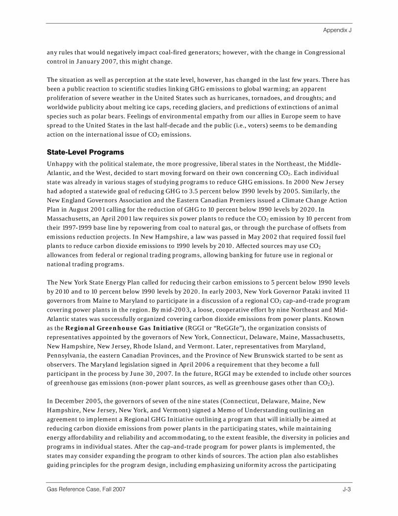
Appendix J
Gas Reference Case, Fall 2007 J-3
any rules that would negatively impact coal-fired generators; however, with the change in Congressional control in January 2007, this might change. The situation as well as perception at the state level, however, has changed in the last few years. There has been a public reaction to scientific studies linking GHG emissions to global warming; an apparent proliferation of severe weather in the United States such as hurricanes, tornadoes, and droughts; and worldwide publicity about melting ice caps, receding glaciers, and predictions of extinctions of animal species such as polar bears. Feelings of environmental empathy from our allies in Europe seem to have spread to the United States in the last half-decade and the public (i.e., voters) seems to be demanding action on the international issue of CO2 emissions. State-Level Programs
Unhappy with the political stalemate, the more progressive, liberal states in the Northeast, the Middle-Atlantic, and the West, decided to start moving forward on their own concerning CO2. Each individual state was already in various stages of studying programs to reduce GHG emissions. In 2000 New Jersey had adopted a statewide goal of reducing GHG to 3.5 percent below 1990 levels by 2005. Similarly, the New England Governors Association and the Eastern Canadian Premiers issued a Climate Change Action Plan in August 2001 calling for the reduction of GHG to 10 percent below 1990 levels by 2020. In Massachusetts, an April 2001 law requires six power plants to reduce the CO2 emission by 10 percent from their 1997-1999 base line by repowering from coal to natural gas, or through the purchase of offsets from emissions reduction projects. In New Hampshire, a law was passed in May 2002 that required fossil fuel plants to reduce carbon dioxide emissions to 1990 levels by 2010. Affected sources may use CO2 allowances from federal or regional trading programs, allowing banking for future use in regional or national trading programs. The New York State Energy Plan called for reducing their carbon emissions to 5 percent below 1990 levels by 2010 and to 10 percent below 1990 levels by 2020. In early 2003, New York Governor Pataki invited 11 governors from Maine to Maryland to participate in a discussion of a regional CO2 cap-and-trade program covering power plants in the region. By mid-2003, a loose, cooperative effort by nine Northeast and Mid-Atlantic states was successfully organized covering carbon dioxide emissions from power plants. Known as the Regional Greenhouse Gas Initiative (RGGI or “ReGGIe”), the organization consists of representatives appointed by the governors of New York, Connecticut, Delaware, Maine, Massachusetts, New Hampshire, New Jersey, Rhode Island, and Vermont. Later, representatives from Maryland, Pennsylvania, the eastern Canadian Provinces, and the Province of New Brunswick started to be sent as observers. The Maryland legislation signed in April 2006 a requirement that they become a full participant in the process by June 30, 2007. In the future, RGGI may be extended to include other sources of greenhouse gas emissions (non-power plant sources, as well as greenhouse gases other than CO2). In December 2005, the governors of seven of the nine states (Connecticut, Delaware, Maine, New Hampshire, New Jersey, New York, and Vermont) signed a Memo of Understanding outlining an agreement to implement a Regional GHG Initiative outlining a program that will initially be aimed at reducing carbon dioxide emissions from power plants in the participating states, while maintaining energy affordability and reliability and accommodating, to the extent feasible, the diversity in policies and programs in individual states. After the cap-and-trade program for power plants is implemented, the states may consider expanding the program to other kinds of sources. The action plan also establishes guiding principles for the program design, including emphasizing uniformity across the participating
Appendix J
J-4
states; building on existing successful cap-and-trade programs; ensuring that the program is expandable and flexible, allowing other states or jurisdictions to join in the initiative; starting the program simply by focusing on a core cap-and-trade program for power plants; and focusing on reliable offset protocols (i.e., credits for reductions outside of the power sector) in a subsequent design phase. In August 2006, model rules for a cap-and-trade market were released. And in January 2007, after several years of drafting, a 163-page final Regional Greenhouse Gas Initiative Model Rule was issued explaining various definitions, setting standards, and creating a tracking system and holding account for CO2 credits. In the West, the state of California was also moving forward during the 2002-2007 time frame, studying the sources of their emissions and announcing plans in July 2006 to reduce CO2 and other GHG emissions by 25 percent by 2020. In January 2007, the California Public Utility Commission unanimously approved a new emissions standard for long-term power generation either built or delivered into the state, requiring that the emissions profile be no greater than a combined-cycle gas-turbine unit. A level of 1,100 pounds of CO2 per MWh was set to help mitigate climate change. Governor Schwarzenegger had signed into law SB 1368 and Assembly Bill 32 which requires reporting and verification of statewide GHG emissions. In the state of Oregon, their Facility Siting Council set stricter carbon dioxide standards for base load gas plants, non-base load power plants, and non-generating energy facilities at only 0.675 pounds per kWh. Effective September 2003, any new or expanded power plant must reduce its rate to 17 percent below efficient natural gas plants either though greater efficiency or by purchasing allowances. In February 2007, the governors of Washington, Arizona, California, New Mexico, and Oregon created the Western Climate Initiative (WCI) with a long-term commitment to significantly reduce regional GHG emissions. Science suggests that this will require worldwide reductions between 50 and 85 percent in carbon dioxide emissions from current levels by 2050. Since February, the state of Utah and the Canadian provinces of British Columbia and Manitoba also have joined the WCI. Four other U.S. states (Colorado, Kansas, Nevada, and Wyoming), three other Canadian provinces (Ontario, Québec, and Saskatchewan), and one Mexican state (Sonora) are participating as observers to the WCI’s deliberations. Some of these entities, as well as others, may seek to join the WCI as full members in the future. In August 2007, the eight members of the WCI announced that they have established a regional goal to reduce greenhouse gas (GHG) emissions in the West to 15 percent below 2005 levels by 2020. They also agreed to design a multi-sector market-based mechanism, such as a load-based cap-and-trade program, by the end of August 2008 to help reach the goal. Each member will also participate in a multi-state GHG emissions registry. The regional goal combines the individual GHG emissions goals that each WCI member already has set, not replacing members’ individual goals. The WCI members will use the regional goal in the design of the multi-sector market-based mechanism. Also, other U.S. states, tribes, Canadian provinces, and Mexican states that want to join the WCI must have an economy-wide greenhouse gas reduction goal that is consistent with the regional goal, in addition to other factors.
Appendix J
Gas Reference Case, Fall 2007 J-5
Figure J-3 States/Provinces with CO2 Initiatives in Process
SOURCE: Global Energy.
International Also in this time frame, the number of industrialized countries that ratified the Kyoto treaty increased from 15 EU countries to 169 countries as of December 2006. Additional studies linking human activity to climate change were released in the last five years, such as the Stern Review from the UK, putting pressure on more and more countries to ratify Kyoto. The Kyoto Protocol came into force in November 2004 when Russia “ratified” it and triggered the rule where it would come into force (legally binding) after 55 percent of the 1990 carbon dioxide emission levels were covered by signatories. Carbon trading, which had begun in the EU several months earlier in September 2004 in preparation for the implementation of Kyoto, experienced a surge in trading through the end of the year. The European Emission Trading Scheme (ETS) officially started in January 2005 including both futures and cash contracts trading on the International Petroleum Exchange (IPE) in London. The world’s biggest emitter of greenhouse gases, the United States, responsible for a quarter of the world’s carbon emissions, didn’t ratify the Protocol, making the United States and Australia the only countries that have signed but not ratified the Protocol. Canada
Canada signed the Kyoto Protocol in 1998 and, after a Parliamentary debate, formally ratified it in December 2002. The Liberal government at the time agreed to reduce Canadian GHG emissions 6 percent below 1990 levels by 2012. However, in January 2006, a Conservative government was elected whose opinion was that the targets are unrealistic, expensive, and unachievable. Additionally, despite ratifying

Appendix J
J-6
the Protocol, Canadian CO2 emissions have been increasing every year since adoption. In February 2007, the Canadian Environmental Minister announced that Canada would not introduce a carbon tax, would not support launching a Canadian carbon market in Montreal, and would not participate in a foreign carbon market buying credits on the international CO2 market, suggesting that Canada would face “economic collapse” if it did so. Instead, Prime Minister Stephen Harper stated the government would set “enforceable targets” for cuts in CO2 emissions and would support a bill aimed to reduced emissions by 45 percent-65 percent below 2003 levels by 2050. This is quite a departure from their Kyoto criteria of CO2 emissions 6 percent below 1990 levels by 2012.
Current Federal Activity Pressure is mounting on countries that have not ratified the Protocol. Most recently, in February 2007, Jacques Chirac of France demanded that the United States sign both the Kyoto climate protocol and a future agreement that will take effect when the Kyoto accord runs out in 2012 or else face a carbon import tax by all EU countries. The European Union is the largest export market for American goods and the United States is obliged to pay if it does not comply with Kyoto. In 2003, Senators Joe Lieberman (D-CT) and John McCain (R-AZ) had called for a cap-and-trade system for GHG emissions in the United States, modeled after the successful acid rain trading program of the 1990 Clean Air act. Their bill, called the “Climate Stewardship Act,” proposed to cut U.S. emissions to 2000 level by 2010 in the electricity generation, transportation, industrial, and commercial economic sectors. However, the proposal was defeated in the Senate in October 2003 by a vote of 43-55. Several other GHG-reduction bills had been defeated over the years. Many regions of the country not only rely on inexpensive coal-fired plants for most of their generation but also count coal production as a key tax payer; this is true at the corporate level as well as worker level, since coal mining is labor intensive. Figure J-4 Coal Generation as a Percentage of Total Regional Generation
0%
10%
20%
30%
40%
50%
60%
70%
80%
90%
100%
MRO US SPP RFC SERC ERCOT WECC FRCC NPCC
SOURCE: Global Energy.
But the proposed Climate Stewardship bill had achieved relatively widespread notoriety. In mid-2005, Lieberman and McCain modified their proposal to include promotions to develop and deploy low or zero greenhouse gas emitting technologies. However, this bill was defeated 38-60. The new Senate and House
Appendix J
Gas Reference Case, Fall 2007 J-7
political landscape that became effective in January 2007 may make it easier to pass legislation for a cap-and-trade CO2 program within the United States, if not outright ratify Kyoto, thus allowing world-wide trading. The United States still remains a signatory to the United Nations Framework Convention on Climate Change. However, in early February 2007, despite a strongly worded global warming report from the world’s top climate scientists, the Bush administration expressed continued opposition to mandatory reductions in heat-trapping GHGs. Energy Secretary Samuel Bodman warned against “unintended consequences,” including an estimated 5 million U.S. job losses that he said might result if the government requires economy-wide caps on carbon dioxide from the burning of fossil fuels. This job loss figure includes not only tens of thousands of coal mine workers, but also secondary and tertiary effects such as industries that would move overseas for more competitive electric rates, associated service industry losses, etc. It is uncertain which course will be taken since the decision is so steeped in politics. When the Lieberman-McCain bills were defeated in 2003 and 2005, the makeup of the Senate was 55 Republicans, 44 Democrats, and 1 Independent. Currently the makeup is 49 Republicans, 49 Democrats, and 2 Independents (one of which is Senator Lieberman). There is the distinct possibility of a successful 51-49 vote if there are no abstentions; however, if the president were to veto the bill, it does not appear that there would be the necessary two-thirds majority for overriding the veto. If Kyoto is ratified, or more likely a regional trading system such as RGGI or a Western states system is implemented, there would be widespread gas demand impacts across the country. Electric generation is a large and growing market for natural gas, and electric imports into CO2-constrained regions via the transmission grid would change fuel consumption patterns far removed from the RGGI states or California and Oregon. Legislative Initiatives
At least six significant legislative proposals mandating greenhouse gas emissions caps are already under serious consideration in the 110th Congress, including the Lieberman-McCain Senate bill and the Bingaman discussion draft. Key features from the early offerings include: • Climate Stewardship and Innovation Act of 2007 (S. 280) Lieberman (I-CT)-McCain (R-
AZ) : cuts emissions to 65 percent below 2004 levels by 2050; o Earlier versions were voted down in 2003 (43-55) and in 2005 (38-60); o Contains controversial provisions promoting nuclear energy; and o Labeled “the Presidential Bill” since three prominent 2008 presidential candidates (Senators
Obama, Clinton, and McCain) are co-sponsors. • Global Warming Pollution Reduction Act (S. 309) Sanders (I-VT)-Boxer (D-CA) : cuts
emissions to 83 percent below 2004 levels by 2050; o Referred to as the “Gold Standard” by environmentalists and by Senator Boxer herself, given it is
the most aggressive proposal. • Electric Utility Cap and Trade Act of 2007 (S. 317) Feinstein (D-CA)-Carper (D-DE) : cuts
emissions to 41 percent below 2004 levels by 2050; o Focuses solely on cutting emissions from power plants; and o Supported by several electric utilities (e.g., Calpine, Entergy, and PG&E).
• Low Carbon Economy Act on Global Warming, (S-1716) Bingaman (D-NM)-Specter (R-PA): holds emissions to 16 percent above 2004 levels by 2020;

Appendix J
J-8
o The least stringent plan focuses on increasing nuclear power production; and o Proposes a “safety valve” to limit total costs to the U.S. economy.
• Climate Stewardship Act of 2007 (H.R. 620) Olver (D-MA)-Gilchrest (R-MD): cuts emissions to 65 percent below 2004 levels by 2050; o Considered a companion to the Lieberman-McCain plan, though slightly more aggressive on cuts
and slightly less supportive of new technology. • Global Warming Reduction Act of 2007 (S. 485) Kerry (D-MA)-Snowe (R-ME): cuts
emissions to 65 percent below 2004 levels by 2050; o In addition to an economy-wide cap-and-trade system, it promotes standards for vehicle
emissions and fuel: by 2016, all gas stations would be required to have at least one pump selling 85 percent-ethanol blended fuel.
• Discussion Draft (No Docket number) Lieberman (I-CT)-Warner(R-VA): cuts emissions to 10 percent below 2005 levels by 2030; 50 percent below by 2040; and 70 percent below by 2050.
Each bill calls for emissions caps on the six major GHGs: carbon dioxide, methane, nitrous oxide, hydrofluorocarbons (HFCs), perfluorocarbons (PFCs), and sulfur hexafluoride (SF6). In addition, the Sanders/Boxer and Kerry/Snowe bills would allow the EPA to include on the list of GHGs, after notice and comment, “any other anthropogenically emitted gas” that contributes to global warming. With the exception of Feinstein-Carper, each bill contemplates imposing emissions limits on a variety of emission sources within the U.S. economy. Feinstein-Carper would impose emissions caps only on electricity generation facilities. Under the Kerry-Snowe and Sanders-Boxer bills, the EPA would be delegated responsibility for determining the specific sources and industry sectors that would be subject to GHG emissions regulations, focusing on sectors and sources with the greatest GHG emissions or the most cost-effective opportunities to reduce emissions. The Lieberman-McCain bill would regulate electric, industrial, and commercial facilities (e.g., power generation and other large emission sources) that emit 10,000 metric tons or more of GHGs per year as measured in units of carbon dioxide equivalents (CO2e) and entities that refine or import petroleum products for use in transportation or that import PFCs, HFCs and SF6 that, when used, will emit 10,000 metric tons or more of GHGs per year. The Bingaman-Specter bill would focus on coal mines, petroleum refineries, natural gas processors, fossil fuel importers, smelter operators, nitrous oxide emitters, and manufacturers and importers of HFCs, PFCs, and SF6. Each bill gives the administrator some discretion to adjust the emissions targets (e.g., if necessary to be more responsive to climate change or when a specific target or mitigation measure is not technologically feasible). Bingaman-Specter also would allow Congress to review whether the enacted emissions limits and other regulations remain appropriate in light of actions taken by international trading partners so that the U.S. economy does not bear a disproportion share of the global emissions reduction effort. Emission Allowance Allocation and Banking
In an effort to reduce the likelihood of windfall profits alleged to occur when allowances are allocated for free, the bills contemplate the possibility of allocating emissions allowances—at least in part—through the use of an auction allocation system. The Sanders-Boxer, Kerry-Snowe, and McCain-Lieberman bills,
Appendix J
Gas Reference Case, Fall 2007 J-9
respectively, would delegate to the Environmental Protection Agency (EPA), the president or the secretary of commerce and EPA discretion to divide and allocate allowances by auction versus for free. Bingaman-Specter would auction 10 percent of all allowances in 2012 to 2016, with a 2 percent increase per year of auctionable allowances thereafter up to a maximum of 65 percent. The remainder of each year’s allowances would be distributed for free to industry and the states as follows: • Industry (e.g., coal mines, refiners, electricity generators) would receive initially 55 percent of
allowances from 2012 to 2016, but then the allocation would be reduced by 2 percent per year thereafter.
• States would receive 29 percent of allowances from 2012 to 2021 and 30 percent per year going forward.
Feinstein-Carper would auction 15 percent of permits in 2011, increasing the allowances auctioned by 3 percent per year for 2012 to 2031 and 5 percent per year for 2031 to 2036 until 100 percent of allowances are auctioned in 2036. Free permits would be allocated based on generation output from each covered generation facility. Feinstein-Carper also would limit free allowances for new coal generation facilities based on whether the facility uses qualifying advanced clean coal technology. McCain-Lieberman would create an allowance allocation priority for covered sources that have registered GHG emission’s reductions prior to 2012 and to covered sources that have agreed to accelerate their emissions reductions to reach 1990 levels by 2012. The bills provide that funds generated from allowance auctions would be held in trust and used for a variety of initiatives, including research and development on abrupt climate change and clean technology, wildlife restoration, and consumer and business subsidies to offset the adverse economic impact of climate change requirements on such entities. With the exception of Sanders-Boxer, the bills contemplate options that would allow covered sources to bank their allowances for future use. In addition, McCain-Lieberman would allow covered sources to borrow credits earmarked for use one to five years in the future to satisfy up to 25 percent of a current year’s allowance requirement, subject to a 10 percent per year carrying cost reflected as an increase in the tradable allowance submission requirement for the year against which the covered source borrowed the credit. Similarly, Feinstein-Carper would give the EPA discretion to permit generators to borrow credits earmarked for use one to five years in the future to satisfy up to 10 percent of a current year’s allowance requirement, subject to an interest payment (federal short-term rate plus 2 percent) and a reduction in the allowances available to satisfy the future year’s allowance requirements. Bingaman-Specter would implement a “safety valve” provision that would cap the price for allowances and thus help mitigate the cost of complying with the emissions reduction targets. Under the safety valve proposal, the initial price of an allowance would be capped at $7, but would increase by 5 percent per year. If allowance prices hit the applicable safety valve price in a given year, the government would treat such an event as a signal to sell additional allowances to bring prices down and mitigate compliance costs.

Appendix J
J-10
Emissions Allowances in Actual Practice
It is anticipated that a “cap and trade” program with CO2 will work similarly to the environmental adders for SO2 and NOX being tacked onto the price of fuel for specific generation units. The NOX is currently only an adder in the SIP Call states on the East Coast but the following is a sample of the dollar per MMBtu adders on the cost of typical gas, oil, and coal units. The $/MMBtu adder would be multiplied by the unit’s heat rate to determine the impact on the electric cost. Figure J-5 Representative Environmental Adders to Electric Dispatch Cost (Under Specific Pricing Assumptions for NOX, SO2, and CO2)
$0.00
$0.25
$0.50
$0.75
$1.00
$1.25
$1.50
$1.75
$2.00
CombinedCycle GT-
Gas
Peaking GT-Gas
SteamTurbine - Gas
SteamTurbine -
2.5% SulfurCoal with
FGD & SCR
SteamTurbine - 1%Sulfur Resid
SteamTurbine -
1.5% SulfurCoal with
SCR
SteamTurbine -
1.5% SulfurCoal
SteamTurbine -
2.5% SulfurCoal
$ / M
MB
tu
NOx $1000/Ton
SO2 $550/Ton
CO2 $5/Ton
SOURCE: Global Energy.
Expectations
In the Senate, Environment and Public Works Chair Barbara Boxer (D-CA) has tried to dampen expectations of producing comprehensive legislation before 2008. Boxer faces several emissions-cap opponents on her own committee (led by Senator Inhofe (R-OK), who has consistently called global warming a “hoax”), and she acknowledges that her own legislative proposal is unlikely to win support. Instead, she is expected to first concentrate on a “small confidence-building bill” before trying to reach a broader compromise. She has also suggested that it might take several smaller bills, rather than a single large bill, to accomplish her goals. Senate Energy and Natural Resources Committee Chair Bingaman (D-NM) agrees that the Senate will have to move somewhat slowly at first. Meanwhile, in the House, Speaker Pelosi has challenged her committee chairs to produce legislation by early June and to pass legislation by July 4, 2007. House Energy and Commerce Committee Chairman Dingell (D-MI) has publicly indicated he will meet the speaker’s schedule for reporting legislation to the full House of Representatives. However, given the challenging nature of the issue (both the science and the politics) establishing total consensus by the summer was too ambitious a goal.

Appendix J
Gas Reference Case, Fall 2007 J-11
Despite all this activity, it remains unclear whether the 110th Congress will pass final legislation, let alone win President Bush’s signature. With the 2008 presidential election cycle under way and several members of both the House and the Senate already announced as candidates for their parties’ nominations, sources indicate that this Congress faces a challenging time crunch as the election nears and monopolizes more and more of its time and energy. By 2008, controversial legislation such as this might have little chance of getting through what will by then be a very distracted and divided Congress; 2007 may be the unofficial deadline for any substantive climate change legislation. Transition to RGGI or other State GHG Programs
The bills are silent on whether federal climate change laws would pre-empt state or regional program requirements like those being implemented in California and the West, and New York and New England (e.g., RGGI).

Appendix K Herfindahl-Hirschman Index
Gas Reference Case, Fall 2007 K-1
The Herfindahl-Hirschman Index (or “HHI”) is a measure of market concentration that is accepted by FERC under the authority of the EPAct 2005 in economic analysis as an indicator of competition. The index takes into account the relative size and distribution of the firms in a market and approaches zero when a market consists of a large number of firms of relatively equal size. The HHI increases both as the number of firms in the market decreases and as the disparity in size between those firms increases. The HHI is calculated by squaring the market share of each firm competing in the market and then summing the resulting numbers. For example, in a market consisting of four firms with market shares of thirty, thirty, twenty, and twenty percent, the HHI is 2600 (302 + 302 + 202 + 202 = 2600). In a market consisting of eight firms with market shares of twenty-five, twenty-two, fifteen, twelve, eight, seven, six, and five percent, the HHI is 1662 (252 + 222 + 152 + 122 + 82 + 72 + 62 + 52 = 1662). In an atomistic market consisting of a thousand firms with market shares of 0.1 percent each, the HHI is 10 (0.12 + 0.12 + 0.12 + ….0.12 = 10). The numeric range of the Herfindahl-Hirschman Index is from 10,000 (in the case of a pure monopoly, e.g., 10,000 = 1002) to a number approaching zero (as in the case of an atomistic or fully competitive market). Markets in which the HHI is in excess of 1,800 points are considered to be concentrated (the first example above). A market such as the one with an HHI above 2,500 is often called an oligopoly, which is a market in which sellers are so few that the actions of any one of them will materially affect price and have a measurable impact on competitors. In fact, the competitors may follow the lead of the major firm in the industry. An example of this is the American auto industry from about 1950-1975 when General Motors had an average market share of over 50 percent and three other U.S. automakers (Ford, Chrysler, and American Motors) had most of the remainder. Markets in which the HHI is between 1,000 and 1,800 points are considered to be moderately concentrated (the second example above). Markets where the HHI is close to zero (the third example above) are considered to be fully competitive and are sometimes called a pure competitor. Transactions that increase the HHI by more than 100 points in concentrated markets presumptively raise antitrust concerns under the Horizontal Merger Guidelines issued by the U.S. Department of Justice and the Federal Trade Commission.
Related Documents