NATURAL GAS POWER GENERATION IN THE PRESENCE OF WIND

NATURAL GAS POWER GENERATION IN THE PRESENCE OF WIND:

A MIXED INTEGER LINEAR PROGRAMMING

APPROACH TO THE HOUR-AHEAD UNIT COMMITMENT PROBLEM

STEVEN H. CHEN

ADVISOR: PROFESSOR WARREN B. POWELL

JUNE 2012

SUBMITTED IN PARTIAL FULFILLMENT

OF THE REQUIREMENTS FOR THE DEGREE OF

BACHELOR OF SCIENCE IN ENGINEERING

DEPARTMENT OF OPERATIONS RESEARCH AND FINANCIAL

ENGINEERING

PRINCETON UNIVERSITY

I hereby declare that I am the sole author of this thesis.

I authorize Princeton University to lend this thesis to other institutions or individuals for

the purpose of scholarly research.

________________________

Steven H. Chen

I further authorize Princeton University to reproduce this thesis by photocopying or by

other means, in total or in part, at the request of other institutions or individuals for the

purpose of scholarly research.

________________________

Steven H. Chen

iii  

Abstract

Power generation is complex because available wind and demand for electric

power are each stochastic and difficult to forecast accurately. The power output of coal

generators is difficult to change in a short time horizon due to their long minimum warm-

up times. Wind is too volatile to be a dependable, short-horizon source of power.

Regional Transmission Organizations such as PJM Interconnection, therefore, turn to

natural gas as an effective source of short-term power. This thesis focuses on hour-ahead

optimization of natural gas generators to supplement day-ahead coal and wind generation.

A mixed integer linear programming approach is used to solve the hour-ahead unit

commitment problem, which gives an adjusted generation schedule in five minute

increments. When the amount of wind power in the system is increased from 5.2% to

20.4% to 40.0%, generation costs decrease and shortage penalties generally increase. A

heuristic that increases the effective horizon of the model decreases the total cost. This

thesis illustrates how PJM can operate its power market more efficiently while increasing

its use of wind power.

iv  

Acknowledgements

First and foremost, I would like to thank and express my gratitude to my advisor

Professor Warren Powell for introducing me to the hour-ahead problem and placing his

trust in me. He guided me and provided insight at every stage of the process. I have

been fortunate to experience first-hand both the level of dedication he shows to his

advisees and his commitment to undergraduate education.

Secondly, I would like to thank Professor Hugo Simão for the time and effort he

spent patiently helping me with the coding process. I am constantly amazed by his ability

to explain in ordinary language even the most complex of problems, and this thesis would

not have been possible without his guidance and reasoning.

Thirdly, I would like to thank Dr. Boris Defourny and Zachary Feinstein for their

helpful suggestions during the coding process. I would like to acknowledge Professor

Hans Halvorson for his input, as well as Ted Borer, Mike Kendig, and Neil MacIntosh for

their insight on natural gas generation. A special thank you goes to Professor Michael

Coulon not only for his suggestions, but also for being a wonderful teacher and mentor.

I would like to acknowledge Kevin Kim and Ahsan Barkatullah for answering my

questions about the prior code, as well as Armando Asunción-Cruz, Phillips Cao, Oleg

Lazarev, and James Luo for their suggestions during the writing process. I would like to

thank Isabella Chen, Celina Culver, Angela Jiang, James Luo, and Ophelia Yin for their

contributions during the editing process. I would like to thank my family and friends for

supporting me. Finally, I would like to thank my parents for their love and

encouragement and for always believing in me.

v  

To Mom and Dad

vi  

Contents

 Abstract .............................................................................................................................. iii

 Acknowledgements ............................................................................................................ iv

 List of Tables .......................................................................................................................x

List of Figures .................................................................................................................... xi

 1 Introduction to the Hour-Ahead Unit Commitment Problem   ...............................1

 1.1 PJM’s Two-Phase Problem  ....................................................................................................2

1.1.1  The Day-Ahead Problem .............................................................................. 2 

1.1.2  The Hour-Ahead Problem ............................................................................. 4 

 1.2 The Impact of Wind Power: 20% Wind by 2030  ............................................................4

1.2.1  Potential Benefits .......................................................................................... 5 

1.2.2  Implications for RTOs .................................................................................. 7 

 1.3 Review of the Unit Commitment Problem  ........................................................................8

1.3.1  Common Objective Functions and Constraints ............................................ 8 

1.3.2  Classes of Algorithm................................................................................... 10 

1.3.3  Justification of Mixed Integer Linear Programming .................................. 11 

 1.4 Overview of Thesis  .................................................................................................................12

 2 Details of Natural Gas Generators   ..........................................................................16

 2.1 Slow versus Fast Generation  ................................................................................................17

 2.2 Combustion Turbine Generators  .........................................................................................19

 2.3 Combined Cycle Generators  ................................................................................................21

2.3.1  Comparison of Efficiency ........................................................................... 22 

2.3.2  The Operation of Combined Cycle Generators .......................................... 22 

2.3.3  Reducing Boiling Time ............................................................................... 26 

 3 The Hour-Ahead Model   ...........................................................................................28

 3.1 Assumptions  ..............................................................................................................................28

vii  

 3.2 List of Variables  .......................................................................................................................31

 3.3 Model  ...........................................................................................................................................34

3.3.1  State Variable .............................................................................................. 34 

3.3.2  Decision Variables ...................................................................................... 35 

3.3.3  Exogenous Information ............................................................................... 36 

3.3.4  Transition Functions ................................................................................... 37 

3.3.5  Objective Function ...................................................................................... 42 

 3.4 Constraints  ..................................................................................................................................43

3.4.1  Upper and Lower Bound Constraints ......................................................... 44 

3.4.2  Intra-Hour Constraints ................................................................................ 45 

3.4.3  Inter-Hour Transition Constraints ............................................................... 50 

3.4.4  Initial Hour Constraints............................................................................... 53 

 3.5 Proposal to Model Combined Cycle Generators  ...........................................................54

3.5.1  Assumptions for Combined Cycle Generators ........................................... 54 

3.5.2  Variables and Parameters for Combined Cycle Generators ....................... 55 

3.5.3  Constraints for Combined Cycle Generators .............................................. 56 

3.5.4  Parameter Constraints for Combined Cycle Generators ............................. 57 

 4 The Simulation Model   ..............................................................................................59

 4.1 Assumptions from the Day-Ahead Model  .......................................................................60

 4.2 List of Variables  .......................................................................................................................61

 4.3 Model  ...........................................................................................................................................67

4.3.1  State Variable .............................................................................................. 68 

4.3.2  Decision Variables ...................................................................................... 69 

4.3.3  Exogenous Information ............................................................................... 70 

4.3.4  Transition Functions ................................................................................... 71 

4.3.5  Objective Function ...................................................................................... 74 

 5 Simulation Data   ........................................................................................................76

 5.1 Generator Data  ..........................................................................................................................77

 5.2 Demand Data  .............................................................................................................................78

 5.3 Wind Data  ..................................................................................................................................80

viii  

 6 Results and Analysis   .................................................................................................82

 6.1 5.2% Wind  ..................................................................................................................................82

6.1.1  The Advantages of Hour-Ahead Rescheduling .......................................... 82 

6.1.2  Explanation of Shortages ............................................................................ 86 

6.1.3  Distribution of Generated Power ................................................................ 88 

6.1.4  Percentage Difference in Overages and Shortages ..................................... 89 

6.1.5  Average and Instantaneous Generator Status ............................................. 91 

 6.2 5.3% Wind with Brownian Bridge Simulation  ..............................................................93

6.2.1  Methodology ............................................................................................... 93 

6.2.2  Results ......................................................................................................... 95 

 6.3 20.4% Wind  ...............................................................................................................................99

 6.4 40.0% Simulation  ..................................................................................................................102

 6.5 Comparison of Wind Penetration Simulations  ............................................................104

6.5.1  Shortages and Overages ............................................................................ 105 

6.5.2  Cost ........................................................................................................... 106 

6.5.3  Generator Status ........................................................................................ 107 

 7 Designing and Testing a Horizon-Increasing Heuristic   ......................................108

 7.1 Revisiting the Horizon Problem  .......................................................................................108

 7.2 Designing a Heuristic to Increase the Horizon  ...........................................................110

 7.3 5.2% Simulation with Heuristic  .......................................................................................112

 7.4 20.4% Simulation with Heuristic  .....................................................................................116

 7.5 40% Simulation with Heuristic  ........................................................................................119

 7.6 Comparison of Heuristic Simulations  ............................................................................123

 7.7 Generalization using a Tunable Parameter  ...................................................................126

 7.8 Proposal to Increase the Horizon of the Hour-Ahead Model  .................................130

7.8.1  State Variable ............................................................................................ 131 

7.8.2  Decision Variables .................................................................................... 132 

7.8.3  Exogenous Information ............................................................................. 132 

7.8.4  Transition Functions ................................................................................. 133 

7.8.5  Objective Function .................................................................................... 135 

ix  

 8 Conclusions and Extensions   ...................................................................................137

 8.1 Results and Implications  ....................................................................................................137

8.1.1  Increasing Wind Penetration ..................................................................... 137 

8.1.2  Increasing the Horizon .............................................................................. 138 

 8.2 Limitations  ..............................................................................................................................139

 8.3 Extensions and Further Areas of Research  ...................................................................140

 8.4 Final Remarks........................................................................................................................142

References   .......................................................................................................................143

x  

List of Tables

Table 1-1: Classes of Algorithms for Unit Commitment .................................................. 10 

Table 2-1: Costs and Efficiency by Generator Type (Boyce, 2010) ................................. 22 

Table 3-1: List of Variables for Hour-Ahead Model ........................................................ 32 

Table 4-1: List of Variables for Simulation Model .......................................................... 63 

Table 5-1: Generator Distribution in Simulations ............................................................ 76 

Table 6-1: Shortages and Overages with Brownian Bridge (5.3%) .................................. 98 

Table 6-2: Cost Distribution with Brownian Bridge (5.3%) ............................................. 98 

Table 6-3: Changes in Generation with Brownian Bridge (5.3%) .................................... 99 

Table 6-4: Shortages and Overages (5.2%, 20.4%, 40.0%) ............................................ 105 

Table 6-5: Cost Distribution (5.2%, 20.4%, 40.0%) ....................................................... 106 

Table 6-6: Generator Status (5.2%, 20.4%, 40.0%) ........................................................ 107 

Table 7-1: Shortages and Overages with Heuristic (5.2%) ............................................. 115 

Table 7-2: Cost Distribution with Heuristic (5.2%) ........................................................ 116 

Table 7-3: Shortages and Overages with Heuristic (20.4%) ........................................... 119 

Table 7-4: Cost Distribution with Heuristic (20.4%) ...................................................... 119 

Table 7-5: Shortages and Overages with Heuristic (40%) .............................................. 122 

Table 7-6: Cost Distribution with Heuristic (40%) ......................................................... 122 

Table 7-7: Shortages and Overages (5.2%, 20.4%, 40%) ............................................... 123 

Table 7-8: Cost Distribution with Heuristic (5.2%, 20.4%, 40%) .................................. 124 

Table 7-9: Changes in Fast Generation with Heuristic (5.2%, 20.4%, 40%) ................. 125 

Table 7-10: Shortages and Overages with Tunable Parameter (40%) ............................ 128 

Table 7-11: Cost Distribution with Tunable Parameter (40%) ....................................... 128 

Table 7-12: Changes in Fast Generation with Tunable Parameter (40%) ...................... 129 

xi  

List of Figures

Figure 1-1: Diagram of PJM’s Service Territory (PJM, 2012) ........................................... 2 

Figure 1-2: Forecasted vs. Actual Demand (California ISO, 2012) ................................... 3 

Figure 1-3: Future Generator Breakdown by Fuel Type (Berst, 2011) .............................. 5 

Figure 1-4: Potential Wind Penetration by State by 2030 (20% Wind, 2008) ................... 6 

Figure 1-5: PJM’s Hunterstown Combined Cycle Power Plant in PA (GenOn, 2010) .... 13 

Figure 2-1: Increase in Natural Gas Consumption (Berst, 2011) ..................................... 18 

Figure 2-2: Components of Combustion Turbine (Fossil, 2011) ...................................... 19 

Figure 2-3: Components of Combustion Turbine Power Plant (Tennessee, 2011) .......... 20 

Figure 2-4: Components of Combined Cycle Power Plant (Shepard, 2010) .................... 21 

Figure 2-5: Diagram of Heat Recovery Steam Generator (Victory Energy, 2011) .......... 24 

Figure 2-6: Steam Turbine Component of Combined Cycle (Combs, 2012) ................... 26 

Figure 2-7: Benefits of Start-up on the Fly Technology (Henkel, 2008) .......................... 27 

Figure 5-1: Actual Demand vs. Predicted Demand .......................................................... 79 

Figure 5-2: Actual Demand vs. Predicted Demand (Zoomed) ......................................... 79 

Figure 5-3: Actual Wind vs. Predicted Wind .................................................................... 81 

Figure 5-4: Actual Wind vs. Predicted Wind (Zoomed) ................................................... 81 

Figure 6-1: Planned Power vs. Predicted Demand (5.2%) ............................................... 83 

Figure 6-2: Planned Power vs. Predicted Demand (Zoomed, 5.2%) ................................ 84 

Figure 6-3: Planned Power vs. Actual Demand (5.2%) .................................................... 85 

Figure 6-4: Actual Power vs. Actual Demand (5.2%) ...................................................... 85 

Figure 6-5: Actual Power vs. Actual Demand (Zoomed, 5.2%) ....................................... 86 

Figure 6-6: Explanation of Shortage (5.2%) ..................................................................... 87 

Figure 6-7: Slow Power vs. Fast Power (5.2%) ................................................................ 89 

Figure 6-8: Percentage Difference (5.2%) ........................................................................ 90 

Figure 6-9: Percentage Difference vs. Actual Wind (5.2%) ............................................. 90 

Figure 6-10: Distribution of Generator Status (5.2%) ...................................................... 91 

xii  

Figure 6-11: Status of Generator 28 (5.2%) ...................................................................... 92 

Figure 6-12: Actual Wind with Brownian Bridge (5.3%) ................................................ 96 

Figure 6-13: Percentage Difference with Brownian Bridge (5.3%) ................................. 97 

Figure 6-14: Actual Wind (20.4%, 5.2%) ....................................................................... 100 

Figure 6-15: Slow Power vs. Fast Power (20.4%, 5.2%) ............................................... 100 

Figure 6-16: Percentage Difference vs. Actual Wind (20.4%) ....................................... 101 

Figure 6-17: Percentage Difference (20.4%, 5.2%) ........................................................ 102 

Figure 6-18: Actual Wind (40.0%, 20.4%, 5.2%) .......................................................... 103 

Figure 6-19: Slow Power vs. Fast Power (40.0%, 5.2%) ............................................... 103 

Figure 6-20: Percentage Difference (40.0%, 20.4%, 5.2%) ........................................... 104 

Figure 7-1: Explanation of Shortage (40.0%) ................................................................. 109 

Figure 7-2: Slow Power with Heuristic (5.2%) .............................................................. 113 

Figure 7-3: Fast Power with Heuristic (5.2%) ................................................................ 114 

Figure 7-4: Percentage Difference with Heuristic (5.2%) .............................................. 115 

Figure 7-5: Fast Power with Heuristic (20.4%) .............................................................. 117 

Figure 7-6: Percentage Difference with Heuristic (20.4%) ............................................ 118 

Figure 7-7: Fast Power with Heuristic (40%) ................................................................. 121 

Figure 7-8: Percentage Difference with Heuristic (40%) ............................................... 121 

Figure 7-9: Percentage Difference with Tunable Parameter (40%) ................................ 127 

1  

Chapter I

1 Introduction to the Hour-Ahead Unit Commitment Problem

In 2010, total domestic energy production in the U.S. was 22.1 trillion kilowatt

hours, of which 17.2 trillion kW·h came from fossil fuel sources and 2.3 trillion kW·h

came from renewable energy sources (U.S. EIA, 2012). Of fossil fuel production, about

37.75% came from natural gas sources and 37.71% from coal sources. In addition,

domestic energy production is projected to grow by a compound annual growth rate of

almost 1.09% from 2010 through 2025, reaching 26.0 trillion kW·h. During this 15 year

time period, energy production from coal sources is forecasted to increase by 1.9% and

energy production from natural gas sources by 20.5%. Energy is crucial to the

functioning of the U.S. economy, with total consumption in 2010 equivalent to about

19.3% of real GDP measured in 2010 dollars (U.S. EIA, 2012; Bureau, 2010).

Energy consumption in the U.S. is dependent on regional transmission

organizations (RTOs), which are power grid operators that are responsible for

coordinating the generation and sale of electric power across interstate borders. RTOs

create a daily generation schedule that determines how much power each generator in the

system must produce to ensure that consumers have enough to use on a daily basis. One

such operator is PJM Interconnection LLC (PJM), which was founded in 1927 and

became the nation’s first fully functioning RTO in 2001.

2  

An independent and neutral party, PJM oversees and operates a competitive

wholesale power market that consists of about 1000 nuclear, coal, hydro, and gas

generators. PJM also maintains the higher-voltage transmission grid that covers 13 Mid-

Atlantic states and the District of Columbia, which provides electricity to over 58 million

people (PJM, 2012). Figure 1-1 illustrates the extent of PJM’s service territory. This

thesis focuses on how PJM creates and adjusts its daily generation schedule to satisfy

consumer demand while minimizing total cost.

Figure 1‐1: Diagram of PJM’s Service Territory (PJM, 2012) 

1.1 PJM’s Two-Phase Problem

PJM’s operation of the electric power market consists of two phases. This section

describes each phase and explains why PJM’s approach to solving the problem may have

to change due to the projected increase in wind power usage.

1.1.1 The Day-Ahead Problem

In the first phase of simultaneous optimal auction, each generator operator in the

PJM network submits a bid indicating the minimum price at which it is willing to

generate power for the following day. Operators submit different bids based on

parameters inherent to each generator. These parameters include, but are not limited to,

3  

the maximum and minimum output capacities, the variable cost for supplying power

(which depends on the generator’s fuel type), and the ramp rate (i.e. the maximum hourly

increase in MW production). PJM takes these factors into consideration and creates a

schedule for the following day that indicates which generators will turn on each hour and

how much power they will produce. PJM makes this schedule by solving the unit

commitment problem, which can be formulated as a mixed integer problem where the

objective is often to minimize total system costs of generation (Yan and Stern, 2002).

This problem is also known as the day-ahead problem.

The day-ahead problem is stochastic due to the uncertain nature of demand. PJM

creates the generation schedule to satisfy predicted consumer demand for electric power,

but due to weather or other random fluctuations, actual demand in the following day may

be different from forecasted demand. Figure 1-2 shows the difference between

forecasted and actual demand, where the dotted purple line represents the day-ahead

forecast, the dotted turquoise line represents the hour-ahead forecast, and the solid blue

line represents actual demand.

Figure 1‐2: Forecasted vs. Actual Demand (California ISO, 2012)

4  

1.1.2 The Hour-Ahead Problem

Due to the difference between actual and predicted demand, PJM must adjust its

day-ahead schedule in real-time to avoid shortages and displeased consumers. The

process of real-time adjustment is the second phase of PJM’s problem. It is also known

as the hour-ahead problem. PJM makes adjustment decisions every five minutes, turning

on or off the fast generators to make up the difference between actual and forecasted

demand (Botterud et al., 2010). To minimize total system costs, PJM satisfies demand by

using the cheapest generators that are able to operate within these short time horizons.

When demand forecasts are relatively accurate, PJM avoids brownouts and unhappy

consumers. The stochastic nature of the hour-ahead problem, however, increases

significantly when PJM allocates larger portions of the generation schedule to wind

power. Accurate wind forecasts are harder to obtain than demand forecasts as wind is

more volatile. But since the U.S. Energy and Information Administration forecasts wind

generation capacity to grow at an annual rate of 2.2% between 2010 and 2025, RTOs

such as PJM must improve their methods of solving the day-ahead and hour-ahead

problems (2012).

1.2 The Impact of Wind Power: 20% Wind by 2030

In 2008, the U.S. Department of Energy published a report studying whether wind

could feasibly account for 20% of the total U.S. power supply by 2030. This percentage

of wind integration into the power supply is called wind penetration. Wind accounted for

11.5% of renewable energy production in 2010 but only 1.2% of total energy production

(U.S. EIA, 2012). The use of renewable energy for power generation, however, is on the

5  

rise. The U.S. Energy Information Administration projects total renewable energy

generation to grow at an annual rate of 1.1% from 2010 to 2025 to 148.42 GW (2012).

Figure 1-3 shows the breakdown by fuel type of North American generators that are

under construction in 2011; the x-axis indicates the year in which a generator will first go

online and the y-axis represents total capacity.

Figure 1‐3: Future Generator Breakdown by Fuel Type (Berst, 2011) 

1.2.1 Potential Benefits

The 2008 Department of Energy report assumes that U.S. electricity consumption

will increase 39% from 2005 to 2030. It also assumes that by 2030 wind turbine energy

production will increase by 15% and turbine costs will decrease by 10%, while costs and

performance levels of fossil fuel technologies stay constant. Achieving the 20%

benchmark would require U.S. wind generation capacity to increase from 11.6 gigawatts

(GW) in 2006 to 305 GW in 2030 (U.S. DOE, 2008). In contrast, total wind generation

capacity currently is projected to reach only 57 GW by 2030 (U.S. EIA, 2012).

6  

Reaching the 20% benchmark does not incur significant marginal costs. Even if

wind generation capacity is not increased, additional infrastructure is nonetheless needed

to satisfy the growth in electricity consumption by 2030. The marginal cost of increasing

wind capacity is $43 billion, or approximately $0.50 per household per month (U.S.

DOE, 2008).

On the other hand, increasing wind penetration to 20% by 2030 would reduce

carbon emissions by 825 million tons per year, which would save between $50 and $145

billion in regulatory costs. The plan would lead to an eight percent reduction in water

consumption – cumulatively saving four trillion gallons of water – as well as an 11%

reduction in nationwide use of natural gas power and an 18% reduction in coal power.

Figure 1-4 shows how 46 states will have established substantial wind presence

by 2030 under the plan and how eight states will each have wind capacity greater than ten

GW. The concentration of offshore wind farms (denoted by the blue icons) along the

Mid-Atlantic is consistent with Google’s recent investment in the Atlantic Wind

Connection, which is a proposed transmission backbone along the Mid-Atlantic that will

connect future offshore wind farms (Wald, 2010).

Figure 1‐4: Potential Wind Penetration by State by 2030 (20% Wind, 2008) 

7  

Wind is a promising source of renewable energy. Regardless of whether the plan

is implemented, wind will play an increasingly large role in U.S. power generation. PJM

and other RTOs, therefore, must improve their unit commitment models, which are

essential to the efficient operation of an electric power market.

1.2.2 Implications for RTOs

The integration of more wind power into the power grid would require operational

changes because “other units in the power system have to be operated more flexibly to

maintain the stability of the power system” (Barth et al., 2006). With offshore wind, for

example, the expansion of transmission grids in remote regions would be necessary to

avoid bottlenecks in wind power delivery. In addition, the system may require more

spinning reserves – the ability of online backup generators to produce power at an

instant’s notice – in case the wind suddenly disappears. These uncertainties would lead

to shifts in supply and demand and affect market clearing prices (Barth et al., 2006).

Wind volatility is not just a problem in the literature; it already has significant

real-life implications. Texas, for example, currently has about 10 GW of wind generation

capacity, but it sometimes provides only 0.88 GW of power (Bryce, 2011). The large

volatility of wind increases the difficulty of the day-ahead and hour-ahead problems.

RTOs may need to create generation schedules in which the total output varies between

extreme values in short amounts of time in order to mimic wind fluctuations.

The bigger problem, however, is the unpredictability of wind. If wind were

volatile but deterministic, solving the unit commitment model would create an effective

schedule given enough generators. But because current wind forecasts are inaccurate,

8  

solving the day-ahead problem is not enough. To understand why, it is useful to conduct

a literature review of the unit commitment problem.

1.3 Review of the Unit Commitment Problem

Padhy defines unit commitment as the “problem of determining the schedule of

generating units within a power system, subject to device and operating constraints”

(2004). Methods of solving the problem range from simplistic approaches such as brute

force, in which all possible solutions are listed and the best is chosen, to new algorithms

such as shuffled frog leaping, an evolutionary algorithm with an especially high

convergence speed (Ebrahimi et al., 2011). Although the unit commitment problem

experiences ongoing research activity, all algorithms for the problem involve optimizing

an objective function subjective to multiple constraints.

1.3.1 Common Objective Functions and Constraints

In the literature, the objective of the unit commitment model is usually to

minimize total system costs of generation (Padhy, 2004):

min , , ,

Here, , is the output of generator at time , , , is the cost of generator

outputting , , and , is the fixed cost of generator at time . The system has

generators, and the problem is solved for time periods. The costs associated with

, include the fuel cost, which is normally modeled as a quadratic, and the

maintenance cost, which is usually linear. Fixed cost , typically includes start-up costs

9  

and shut-down costs. The constraints typically involve the generators’ minimum online

times, minimum off times, and maximum ramp rates (Padhy, 2004).

Alternatively, in the case of deregulated electricity markets, the objective function

can be to maximize profit (Padhy, 2004):

max , , , , , ,

Here, , is the time zero forecasted price of generator ’s incremental output at

time and , is an indicator variable that is equal to 1 when generator is online at

time and 0 otherwise. The expression , , , refers to the revenue earned by

generator at time , and the expression in parenthesis is the operating cost from the prior

formulation (Padhy, 2004). The constraints are the same as before. In either case, the

problem can be augmented with grid constraints that restrict the amount of output

flowing from a generator in one location to the demand in another location. The

implementation of grid constraints requires additional information about the distances

and maximum flow capacities between generator and demand locations.

Yan and Stern propose an objective function that uses the marginal clearing price

, which is independent of generator (2002):

min , ,

Here, , is the startup cost of generator at time , and is the maximum time

fuel cost for generator over the set of all online generators at time . This objective

function analyzes the problem from the perspective of the market clearing price instead

10  

of the traditional bid price. A limitation of this functional form is that it loses the

separable structure required by the common Lagrangian relaxation algorithm.

1.3.2 Classes of Algorithm

The unit commitment problem is a mixed integer, nonlinear problem with many

approximate solutions (Chang et al., 2004). Padhy classified common algorithms for the

problem into 16 types (2004):

Table 1‐1: Classes of Algorithms for Unit Commitment 

1. Exhaustive Enumeration

2. Priority Listing

3. Dynamic Programming

4. Linear Programming

5. Branch and Bound

6. Lagrangian Relaxation

7. Interior Point Optimization

8. Tabu Search

9. Simulated Annealing

10. Expert Systems

11. Fuzzy Systems

12. Neural Networks

13. Genetic Algorithms

14. Evolutionary Programming

15. Ant Colony Search

16. Hybrid Models

In practice, the most commonly used classes are priority listing, linear

programming, and Lagrangian relaxation, perhaps due to their limited complexity and

ease of implementation. Priority listing creates a list of all generators sorted from least

expensive fuel cost to most expensive fuel cost; the algorithm ramps up the output of the

cheapest generators until demand is satisfied. Linear programming approximates the

objective function and constraints as linear functions and constraints, which reduces the

problem to a linear optimization problem. Lagrangian relaxation rewrites the constraints

using Lagrange multipliers to add penalty terms, and the algorithm relaxes successive

11  

constraints to reach an optimal solution. Lagrangian relaxation traditionally has been the

most common method because it is easy to customize individual constraints for

generators with unique characteristics, but it is not the method used in this thesis (Padhy,

2004).

1.3.3 Justification of Mixed Integer Linear Programming

The issue of size typically has hindered the use of linear programming to solve the

unit commitment problem, since in the worst case scenario the running time is .

The development of more efficient optimization packages, however, has refueled interest

in both linear programming and mixed integer linear programming, which is linear

programming using a mixture of integer and non-integer variables. Advantages of using

mixed integer linear programming include the relatively noncomplex process of

linearizing the constraints and the use of dual variables to give additional information on

pricing (Chang et al., 2004).

This thesis, therefore, formulates the hour-ahead unit commitment problem as a

mixed integer linear program. Code written in JAVA creates the linear program and calls

the optimization package CPLEX to solve it. The notation for this thesis’s model comes

from Chang et al.’s formulation, which minimizes system costs while writing constraints

as linear equations with integer variables (2004).

Consider as an example the constraint that prevents generator from turning on

and off at the same instant. Let , be an indicator variable that is 1 when generator is

online at time and 0 otherwise. Takriti et al.’s traditional Lagrangian relaxation model

implements this constraint by adding a penalty term to the objective function (1996):

, , ,

12  

Here, , is the Lagrangian multiplier, and , is a probability-weighted average

of generator output decisions (Takriti et al., 1996). But the objective function may be

quadratic. In contrast, Chang et al. propose the following linear constraints (2004):

, , , ,

, , 1

Here, , and , are integer variables corresponding to whether generator turns

on or off at the instant , respectively. These constraints ensure that generator cannot

turn on and off at the same time. They are not added to the original objective function,

which stays linear. Jessica Zhou’s senior thesis, which solves PJM’s day-ahead problem

and serves as a starting point for this thesis, also uses Chang et al.’s formulation of linear

constraints (2010; 2004). Zhou, however, uses the priority listing algorithm to solve the

hour-ahead problem (2010). This thesis seeks to make a contribution to the literature by

solving the hour-ahead problem in the presence of wind power through mixed integer

linear programming.

1.4 Overview of Thesis

This chapter introduces PJM’s two-phase problem of simultaneous optimal

auction (the day-ahead problem) and real-time adjustment (the hour-ahead problem). It

also motivates the need to integrate more wind power into PJM’s system and provides a

brief review of the unit commitment problem. Chang et al.’s formulation and Zhou’s

model are used as a starting point, although modifications are needed (2004; 2010).

Zhou uses mixed integer linear programming to solve the day-ahead problem and

a priority listing algorithm to solve the hour-ahead problem (2010). The latter algorithm

13  

sorts each type of generator from least to most expensive fuel cost. Starting with the least

expensive coal generators and ending with the most expensive gas generators, the

algorithm increases the outputs of successively more expensive generators of each type

until actual demand is cleared (Zhou, 2010).

This algorithm, however, fails to take advantage of the cycling speed of natural

gas generators, which can be turned on and off within minutes. Chapter 2 provides an

overview of natural gas generators (both combustion turbine and combined cycle power

plants) and demonstrates their ability to operate on a smaller time scale, a nuance that is

lacking in Zhou’s model:

“The model assumes that at the beginning of each hour, there is a demand deviation, and these demand deviations last for the whole hour. Generators are given only five minutes to ramp up or down to adjust to exogenous demand levels. The generation for the next 55 minutes remains constant until the beginning of the next hour, when new exogenous demand requires portfolio rebalancing again within five minutes.” (Zhou, 2010)

This thesis, therefore, attempts to add to the literature by proposing an hour-ahead

model in Chapter 3 that solves PJM’s hour-ahead problem through mixed integer linear

programming. For each hour of simulation, the hour-ahead unit commitment problem is

solved in 12 five minute increments, which reduces the time scale of the problem to take

advantage of the speed of natural gas generators and, therefore, makes the modeling of

those generators more realistic.

Figure 1‐5: PJM’s Hunterstown Combined Cycle Power Plant in PA (GenOn, 2010) 

14  

This thesis also attempts to add to the literature of the unit commitment problem.

The formulations of Chang et al. and Zhou do not include a generator warm-up state

(2004; 2010). In their models, generators produce zero power only in the off state. In the

real world, however, generators must warm up before they go online and produce their

first MW of power. The hour-ahead model proposed in Chapter 3 requires each

generator to be in exactly one of three states: warming up, online, and off. As a result,

this formulation allows the use of a minimum warm-up time in addition to minimum

online and off times, which provides a more realistic model for natural gas generators.

Chapter 3 also describes the linear constraints required to implement the hour-ahead

model as a mixed integer linear program. A model to include combined cycle generators

in the hour-ahead model is also presented at the end of Chapter 3, intended as a reference

for future research when sufficient data is available.

Chapter 4 presents the mathematical formulation of the simulation model, which

relates the hour-ahead model to its day-ahead counterpart. The chapter explains how the

hour-ahead model fits into the simulation as a whole.

The three sources of data required for the simulation are reviewed in Chapter 5,

which describes where the generator, demand, and wind data are obtained from and how

they are adjusted from the original data for use in the simulation. The chapter also

describes how the wind penetration simulation parameter is calculated.

Chapter 6 analyzes the results of the simulations. Comparisons of shortage and

overage statistics, cost distribution, and generator activity are compared at wind

penetration levels of 5.2%, 20.4%, and 40.0%. Increased wind volatility through the use

of Brownian bridge simulation is also studied at 5.3% wind.

15  

Chapter 7 proposes a heuristic to amend a limitation of the hour-ahead model,

which is explained initially in Chapter 6. The heuristic increases the effective horizon of

the model. It is tested at wind penetration levels of 5.2%, 20.4%, and 39.9%, and the

results are compared to the base case simulations. The heuristic is also generalized by

using a tunable parameter, which is tested at 39.9% wind. A model to increase the

horizon by five minutes without using a heuristic is presented at the end of the chapter,

intended as a reference for future research.

Finally, Chapter 8 summarizes the conclusions of the simulations, describes

limitations of the model, and proposes areas for future research.

16  

Chapter II

2 Details of Natural Gas Generators

Power systems for production of electric power fall into one of four major

categories: fossil fuel power plants (which include coal generators and natural gas

generators), nuclear power plants, hydraulic power plants, and renewable energy power

plants (Boyce, 2010). Natural gas generators can be further separated into two types:

combustion turbine (also called gas turbine or simple cycle) generators and combined

cycle generators.

Different types of generators are used to satisfy different kinds of demand for

power. During the day-ahead bidding process, generators submit a price below which

they are unwilling to generate power. PJM aggregates these bids to form the electric

power supply curve, known as the merit order. Generators with low marginal costs enter

at the bottom of the merit order because they can profit even when the price charged to

consumers is low. More expensive generators enter the merit order at higher prices.

Differences in generators’ marginal cost are largely due to fuel type. Natural gas

generators incur significantly larger variable costs than their coal generator counterparts

(about $ .

compared to $ .

) and therefore appear higher in the merit order because

they demand a higher price to operate (Rebenitsch, 2011).

17  

2.1 Slow versus Fast Generation

Coal generators are often coal-fueled steam power plants that boil water and use

the resulting steam to generate power. These are categorized as slow generators because

they tend to have long warm-up periods due to the time it takes to boil the water. Slow

generators and others at the bottom of the merit order generally serve baseload—the

portion of demand that never falls below a certain baseline even in the early morning or

late evening of the day. Baseload generally comprises 30% to 40% of the maximum load

for a given time period.

Due to their quick startup times and ramp rates, on the other hand, natural gas

generators are categorized as fast generators. They typically are used to satisfy peakload,

the portion of demand that fluctuates highly depending on the time of day. They are

operated in cycling mode because they can complete multiple cycles of turning on and off

in a day and begin generating power on the order of minutes instead of hours.

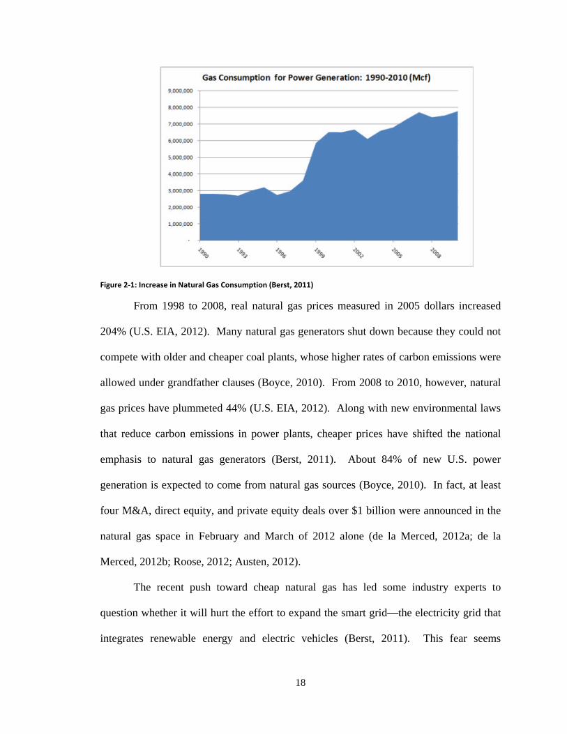
Although they are extremely costly to operate from a marginal perspective,

natural gas generators are less expensive to build (Cordaro, 2008). As shown in Figure 2-

1, they have become more common as sources of power consumption in the last 20 years

due to their lower carbon emissions and their competitive pricing. The y-axis is in

thousands of cubic feet.

18  

Figure 2‐1: Increase in Natural Gas Consumption (Berst, 2011) 

From 1998 to 2008, real natural gas prices measured in 2005 dollars increased

204% (U.S. EIA, 2012). Many natural gas generators shut down because they could not

compete with older and cheaper coal plants, whose higher rates of carbon emissions were

allowed under grandfather clauses (Boyce, 2010). From 2008 to 2010, however, natural

gas prices have plummeted 44% (U.S. EIA, 2012). Along with new environmental laws

that reduce carbon emissions in power plants, cheaper prices have shifted the national

emphasis to natural gas generators (Berst, 2011). About 84% of new U.S. power

generation is expected to come from natural gas sources (Boyce, 2010). In fact, at least

four M&A, direct equity, and private equity deals over $1 billion were announced in the

natural gas space in February and March of 2012 alone (de la Merced, 2012a; de la

Merced, 2012b; Roose, 2012; Austen, 2012).

The recent push toward cheap natural gas has led some industry experts to

question whether it will hurt the effort to expand the smart grid—the electricity grid that

integrates renewable energy and electric vehicles (Berst, 2011). This fear seems

19  

unfounded. Natural gas improves the smart grid by replacing dirtier coal generators, and

their correct usage can help PJM integrate more wind into the system. The following

sections explore the operational details of both types of natural gas generators.

2.2 Combustion Turbine Generators

Combustion turbine generators contain at least one combustion turbine that is

used to burn gas and produce energy. Unlike coal-fueled steam generators, no water is

necessary to turn the turbine, which is instead turned by the force of burning gas. Figure

2-2 depicts a typical combustion turbine.

Figure 2‐2: Components of Combustion Turbine (Fossil, 2011) 

The combustion turbine is similar to a jet engine because it draws air into the

engine through the inlet section, which is then pressurized and injected into the

combustion chamber at high speeds on the order of hundreds of miles per hour. The air

then mixes with the natural gas fuel that is injected into the combustion system. This

high-pressure combination burns at about 2300 °F and flows into the turbine, where the

resulting force rotates the turbine’s airfoil blades. In addition to generating power, the

rotating blades allow waste heat to exit through the exhaust. The higher the temperature

20  

of the combustion turbine generator, the more efficient it is. Some of the critical metal

components of the combustion turbine, however, may only withstand temperatures up to

1700 °F before failing. Some injected air, therefore, is diverted to cool the metal, which

decreases the plant’s efficiency but prolongs its lifespan (Fossil, 2011).

Since it does not require boiling water, combustion turbine generators can go

online and generate power from a cold start in minutes rather than hours. Furthermore,

since there is usually no minimum online time for combustion turbine plants – which

applies to coal plants to protect the equipment – they can be turned off at a moment’s

notice. These characteristics make combustion turbine plants suitable to satisfy peakload,

which often appears and disappears within minutes (Tucker et al., 2009). Figure 2-3

depicts a typical combustion turbine generator.

Figure 2‐3: Components of Combustion Turbine Power Plant (Tennessee, 2011) 

Note that the waste heat generated in the combustion chambers is simply released

from the exhaust. This unused source of energy is the major operational difference

between a combustion turbine generator and a combined cycle generator.

21  

2.3 Combined Cycle Generators

Combined cycle generators have at least one gas turbine and at least one steam

turbine. Unlike combustion turbine generators, these power plants pass the waste heat

from fueling the gas turbine through a heat recovery steam generator to boil water. They

use the resulting steam to spin the steam turbine and generate additional power, after

which the steam is passed through a condenser and transformed back to water for further

steam generation. Combined cycle generators are more efficient than their combustion

turbine counterparts because they use the byproduct heat that would otherwise be wasted.

The gas turbines typically generate about 60% of the total power while the steam turbines

generate 40%, although this ratio depends on the number of turbines (Boyce, 2010).

Figure 2-4 illustrates a typical combined cycle generator.

Figure 2‐4: Components of Combined Cycle Power Plant (Shepard, 2010) 

Combined cycle generators can operate as combustion turbine generators only if

they install a bypass damper that increases the efficiency of waste heat diversion; doing

so without a bypass damper would be inefficient (Kendig, 2011).

22  

2.3.1 Comparison of Efficiency

As shown in Table 2-1, combined cycle generators are more efficient than

combustion turbine generators, which in turn are more efficient than coal generators.

Table 2‐1: Costs and Efficiency by Generator Type (Boyce, 2010) 

Generator Type Variable Costs

($/kW) Fixed Costs

($/kW)Heat Rate

(Btu/kW·h) Net Efficiency

Coal 3.0 1.43 9749 35%

Combined Cycle 4.0 0.35 6203 55%

Combustion Turbine 5.8 0.23 7582 45%

Combined cycle generators were originally designed to satisfy baseload, but they

are better suited to satisfy peakload than coal generators due to their faster ramp rates.

They can cycle between 40% and 100% of maximum capacity in a single day and are

operated with multiple starts (Boyce, 2010). Compared to combustion turbine generators,

however, combined cycle plants are more suited for baseload operation.

2.3.2 The Operation of Combined Cycle Generators

Combined cycle generator operation is illustrated using Gilbert Generating

Station in New Jersey, which is part of PJM. This station has a 288 MW, 4x1 combined

cycle power plant. The generator’s 288 MW capacity refers to the total generation of its

gas and steam turbines. The 4x1 multi-shaft indicator means the combined cycle plant

has four gas turbines powering one steam turbine. Using multiple gas turbines to supply

steam to each steam turbine generally increases the plant’s efficiency.

Combined cycle plants usually have a separate water boiler for each gas turbine.

This design leads to a constant warm-up time for the steam turbine. Regardless of how

many gas turbines are initially switched on, in other words, the demineralized water boils

23  

in the same amount of time because each gas turbine has its own separate boiler. The

steam turbine warm-up time, therefore, is dependably constant, according to Mike

Kendig, the Operations Manager of Hunterstown Generating Station in Gettysburg, PA,

allowing plant operators to know exactly how far in advance they must ignite the gas

turbines in order to become fully online by a certain time (2011).

The output of the steam turbine, however, will be proportional to the number of

online gas turbines. Two online gas turbines will generate half as much steam as four

online gas turbines and, therefore, half as much power through the steam turbine. The

use of separate boilers is indicated by the x x notation, where is the number of

gas turbines, is the number of boilers, and is the number of steam turbines (Kendig,

2011). The Gilbert combined cycle plant, therefore, is 4x4x1.

According to Neil MacIntosh, the Plant Manager of Gilbert Generating Station in

Milford, NJ, the first step in taking a cold combined cycle power plant to full capacity is

to turn on any combination of the gas turbines (2011). Each gas turbine does not

immediately produce any power because it must first warm up. During this time, the gas

fuel is injected at approximately 45 psi and must be pressurized to approximately 400 psi

before the gas turbine can generate power (Borer, 2011). After 15 minutes, each gas

turbine goes online and produces its first MW of power. The online gas turbines can then

be ramped up to their full capacity according to their ramp rates. For example, each of

the four gas turbines in Gilbert Generating Station’s combined cycle power plant has a

ramp rate of 2.5 . The ramping capability of these gas turbines is additive: if exactly

three of the gas turbines are online, the generator’s ramp rate would be7.5 , and if all

four of the gas turbines are online, it would be 10 (MacIntosh, 2011).

24  

Figure 2‐5: Diagram of Heat Recovery Steam Generator (Victory Energy, 2011)

After the boiler warms up, the waste heat from the gas turbines begins to boil the

water. Exiting the gas turbines at almost 1200 °F, the waste heat enters a heat recovery

steam generator pictured in Figure 2-5, where it passes over and heats the tubes that

contain demineralized water. The majority of this heat is used to boil the water, after

which the heat dissipates from the power plant at a considerably lower temperature of

around 200 °F (Kehlhofer et al., 2009). The time required to boil the water and generate

sufficient steam can be interpreted as a warm-up time for the steam turbine. For the

Gilbert Generating Station combined cycle plant, the steam turbine warm-up time is

about 3.5 hours (MacIntosh, 2011). This value generally depends on the steaming

capacity of the power plant, or the amount of generated steam measured in . The

25  

warm-up time is also limited by the boiler’s rate of temperature increase, usually not

exceeding °

(Borer, 2011).

After the water boils, the steam turbine goes online and begins generating power;

it can also be ramped up to its maximum capacity at its ramp rate, which may be different

from the gas turbine’s ramp rate. For example, Gilbert Generating Station’s combined

cycle plant has a steam turbine ramp rate of 2 , 20% lower than that of a gas turbine

(MacIntosh, 2011). After the steam turbine is ramped up to its maximum capacity, the

entire combined cycle plant operates at full capacity.

At least one gas turbine must be online for the steam turbine to be online;

otherwise no steam is available to drive the steam turbine. It is impossible, therefore, to

run only the steam turbine component of the combined cycle plant (MacIntosh, 2011).

When operators reduce the power output of an online combined cycle plant, they

ramp down any number of the gas turbines, which causes the steam turbine to ramp down

simultaneously due to less available generated steam as fuel. Although it is possible for

operators to ramp down only the steam turbine – for example, by flipping a switch to

reduce the amount of steam introduced to the steam turbine – this is not a common

practice (Kendig, 2011). The reason is that zero variable cost is associated with the

steam turbine component of the combined cycle plant because its power generation is

entirely dependent on the gas turbines and requires no additional cost.

To turn off the combined cycle plant, gas turbines are ramped down to minimum

load and subsequently switched off, which causes the steam turbine to be switched off

when it is operating at approximately 15% load. Gradually ramping down the steam

turbine from 15% load to 0% load is avoided, however, to prevent equipment damage.

26  

Figure 2‐6: Steam Turbine Component of Combined Cycle (Combs, 2012)

The gas turbines generally have a minimum online time in order to preserve the

equipment but no minimum off time, allowing the gas turbines to be switched on

instantaneously to satisfy peakload. The steam turbine, on the other hand, generally has a

minimum off time in order to prevent damage to the steam turbine. It has no minimum

online time, however, so given that the gas turbine’s minimum online time is satisfied,

operators may shut down the combined cycle plant during the boiling of the

demineralized water without damaging the equipment (Kendig, 2011).

2.3.3 Reducing Boiling Time

The limiting factor in how quickly a combined cycle plant can reach full capacity

is the boiling time. On the order of six hours for coal generators, the boiling time is

reduced in combined cycle generators when applying a technique known as the “steam

blanket.” When the gas and steam turbines are off, operators pay a cost to keep the

demineralized water at a higher temperature and pressure, which allows it to be boiled

27  

much quicker (MacIntosh, 2011). For example, the combined cycle generator at Gilbert

Generating Station has a 3.5 hour boiling time, which is about 1.5 hours to 2 hours

shorter than what it would be without the use of a steam blanket (MacIntosh, 2011).

Another technology is the “start-up on the fly” method developed by Siemens.

This technique eliminates the steam turbine’s warm-up time by leveraging the cold steam

produced by the heat recovery steam generator in a full temperature and pressure

environment. A single shaft 400 MW combined cycle plant can go from ignition to full

capacity in 40 minutes (Henkel, 2008). Figure 2-7 shows the improvement in combined

cycle start-up time.

Figure 2‐7: Benefits of Start‐up on the Fly Technology (Henkel, 2008)

28  

Chapter III

3 The Hour-Ahead Model

This chapter establishes a mathematical model for the hour-ahead unit

commitment problem. It then transcribes that model using linear constraints to solve it as

a mixed integer linear program. The modeling of combustion turbine generators is

similar to that of coal generators in Jessica Zhou’s senior thesis on the day-ahead problem

(2010). The use of warm-up times, however, changes the necessary constraints.

Based on the study of combined cycle generators in the previous chapter, it is

possible to model these generators as interconnected gas turbine and steam turbine

generators. It is also possible to model them as slow generators because they are

generally used to satisfy baseload. The former method requires separate parameter data

for each component of the combined cycle plant. The available data, however, does not

distinguish between components, so this thesis uses the latter method. The hour-ahead

model established in this chapter, therefore, only applies to fast generators. The last

section of this chapter proposes a separability model for combined cycle generators as a

reference for future research when separate combined cycle data is available.

3.1 Assumptions

Many useful parameters for PJM’s hour-ahead problem are unavailable, and not

all of the available parameters are useful in modeling the problem. Assumptions,

29  

therefore, are required to reduce the dimensionality of the hour-ahead model and

diminish its runtime to strike a balance between realism and efficiency. These

assumptions are listed below.

1. Use of actual demand:

Due to the lack of predicted demand data in five minute increments and the

difficulty of simulating greater dependency between sub-hourly predicted and

actual demand, actual demand is used as input to the hour-ahead model.

Although this implementation allows the model to peek 55 minutes into the

future every hour, an eventual switch to using predicted demand is relatively

straightforward when the data becomes available.

2. Limitations of modeling the system:

Due to lack of data, certain aspects of PJM’s system are not modeled. These

include but are not limited to: supply side offers, transmission and grid

constraints, and battery storage.

3. Limitations of modeling the generators:

Due to lack of parameter data, the hour-ahead model does not include certain

aspects of generators that may appear in the unit commitment literature.

These include but are not limited to: startup and shutdown costs, cold and hot

startup conditions, cool-down state, temperature- and season-dependent

efficiency, output-dependent ramp rates, and actual generation costs (Padhy

2004; MacIntosh, 2011; Kendig, 2011; Kelholfer et al., 2009).

30  

4. No violation of the off – warm-up – online cycle:

In Zhou’s thesis, generators can go online immediately after satisfying

minimum off times (2010). In reality, however, generators must warm up

before generating power, even after satisfying minimum off times (Kendig,

2011). At any given time, this model assumes generators are in exactly one of

the following three states: warming up, online, and off. If a generator is off,

its next state is the warming up state (it cannot directly go online). If a

generator is warming up, its next state is the online state (it cannot directly

turn off). If a generator is online, its next state is the off state (it cannot

directly begin warming up).

5. No reserve requirement:

The North American Electric Reliability Corporation (NERC) standards

recommend reserving a percentage of maximum demand forecasts (Botterud

et al., 2009). The purpose of maintaining reserves is to give generators a

buffer during real-time adjustment in case actual demand greatly exceeds

predicted demand. Since the hour-ahead model uses actual demands, it does

not incorporate reserves.

6. Combined cycle generators are categorized as slow generators:

Due to lack of separate data for the gas turbine and steam turbine components

of combined cycle generators, combined cycle generators are assumed to be

slow generators.

31  

7. Initial state of generators during the first hour of the first day:

All generators are assumed to be off prior to the first time period of

simulation. They have satisfied their minimum off time, so they may begin

warming up during that period but cannot go online. This assumption is

guaranteed by the initial hour constraints.

3.2 List of Variables

This list contains all variables associated with gas generators that are used in the

hour-ahead unit commitment model. Depending on its subscript, each of the following

variables and parameters may exist ∀ ∈ , 1, … , where is the set of all gas

generators and 12 is the number of time increments per hour. In addition, this model

uses a lagged information process. The hour-ahead model schedules decisions at a

certain time, but these decisions are implemented at later times. The variable , , ,

therefore, denotes the information or decision regarding generator that is known or

made at time by the hour-ahead model and is actionable or implemented at time .

32  

Table 3‐1: List of Variables for Hour‐Ahead Model 

Variable Definition Decision Variables  

, ,   Warming up status: is 1 if combustion turbine generator   is warming up at time  ′, is 0 otherwise 

, ,  

Begin  warming  up  indicator:  is  1  if  combustion  turbine generator   begins warming up at time  ′, is 0 otherwise  

, , Online  status:  is  1  if  combustion  turbine  generator    is online at time  ′, is 0 otherwise 

, , Going online indicator: is 1 if combustion turbine generator  goes online at time  ′, is 0 otherwise 

, ,  Turning off indicator: is 1 if combustion turbine generator   turns off at time  ′, is 0 otherwise  

, , Combustion  turbine  generator  ’s  committed  generation (MW) at time   

,   Slack variable representing power shortage at time   

 Generator Parameters

, Variable fuel cost $

 for combustion turbine generator   

at time    

Minimum output (MW) for combustion turbine generator    

Maximum output (MW) for combustion turbine generator    

Minimum  warm‐up  time  in  number  of  increments  for combustion turbine generator  ; set to be  1 

Minimum  online  time  in  number  of  increments  for combustion turbine generator  ; set to be  1 

Minimum off time in number of increments for combustion turbine generator  ; set to be  1 

Ramp‐up rate ( ) for combustion turbine generator   

( 0) 

33  

Ramp‐down  rate  ( )  for  combustion  turbine 

generator   ( 0)    System Parameters  

  Actual  demand  at  time  ′  that  must  be  satisfied  by  fast generators (excludes slow generation and wind power) 

  Penalty $

 for power shortage at time increment   

 Transition Variables   

,   Combustion  turbine  generator  ’s  warming  up  status  at , the last increment of this hour: is 1 if warming up, 0 if 

not warming up  

,   Combustion turbine generator  ’s online status at  : is 1 if online, 0 if not online 

,   Number  of  consecutive  increments  (inclusive)  combustion turbine generator   has been warming up by   

,   Number  of  consecutive  increments  (inclusive)  combustion turbine generator   has been online by   

,   Number  of  consecutive  increments  (inclusive)  combustion turbine generator   has been off by   

,   Whether  combustion  turbine  generator    does  not  satisfy the  minimum  warm‐up  time  at  :  is  1  if  minimum warm‐up time is not yet satisfied, 0 otherwise 

, Whether  combustion  turbine  generator    does  not  satisfy the minimum online  time at  :  is 1  if minimum online time is not yet satisfied, 0 otherwise 

,Whether  combustion  turbine  generator    does  not  satisfy the minimum off time at  :  is 1  if minimum off time  is not yet satisfied, 0 otherwise 

,   Combustion turbine generator  ’s output (MW) at    

34  

3.3 Model

Following Powell’s notation, the hour-ahead problem can be modeled by defining

the state variable, decision variables, exogenous information, transition functions, and

objective function (201). Each component of the model is described below.

3.3.1 State Variable

Powell defines the state variable as the “minimally dimensioned function of

history that is necessary and sufficient to compute the decision function, the transition

function, and the contribution function” (2010). In other words, the state variable

consists of the least amount of information that is necessary and sufficient for the

decision-making process.

Let be the set of all gas generators. Let denote the vector of variables

across all ∈ for a given time , where represents a generic variable that is indexed

by both time and generator. Then the state variable at time for the hour-ahead model

is the following:

, , , , , , , , , , , , , , ,

Together, , and , determine the time continuous state of generator :

whether it is warming up, online, or off (if , and , are both 0, then the generator is

off). Of the three variables , , , , and , , at most one is nonzero.

Similarly, of the three variables , , , , and , , at most one is nonzero.

Since it is not known in advance which is nonzero, the state variable must include all of

these variables to guarantee sufficient information to compute the transition function.

35  

When the hour-ahead model is integrated into the simulation, the state variable is

written as , , where day and hour of the simulation define the time when the

hour-ahead model is called. Chapter 4 explores this notation in further detail.

3.3.2 Decision Variables

The decision variables are chosen at time for each time increment 1, … , .

They are chosen based on a particular policy , which Powell defines as a “rule or

function to determine a decision given the available information in the state ” (2010).

For convenience, the decision variables’ dependence on is not explicitly denoted.

For each time increment, there are six decision variables for each combustion

turbine generator as well as one slack decision variable. These variables determine how

much power each generator supplies at a given time:

, ,1 ′0

, ∀ ∈ , 1, … ,

, ,1 ′0

, ∀ ∈ , 1, … ,

, ,1 0

, ∀ ∈ , 1, … ,

, ,1 ′0

, ∀ ∈ , 1, … ,

, ,1 ′0

, ∀ ∈ , 1, … ,

, , 0, ′, ∀ ∈ , 1, … ,

, , ′, ∀ ∈ 1…

36  

The decision variables are chosen by a decision function Χ that depends on

policy and state variable , where is the time that the function is called. The policy

takes into account the tunable parameters and the algorithm used to solve the hour-ahead

problem (in this case, mixed integer linear programming). The decision function outputs

decision variables for all applicable 1,… , in the time horizon and ∈ . The

relation can be expressed in matrix form as follows:

Χ , , , , , ,

, , , , , ,

, , , , , ,

,

In the simulation model defined in Chapter 4, the hour-ahead model decision

function is written as Χ , , where denotes the hour-ahead model.

3.3.3 Exogenous Information

The random components of this problem are , and , , which are the load

demanded at time and the amount of wind power available at time ,

respectively. Each is random at present time . These values are replaced by actual

demand values and actual wind values may be substituted.

Let be the current slow generation at time from generators that cannot be

adjusted on a sub-hourly basis. Then the effective actual demand that the hour-ahead

model must satisfy is:

As wind power and current slow generation increase, less power is needed to be

generated by the hour-ahead model.

37  

3.3.4 Transition Functions

The transition functions determine each component of the state variable for the

next time increment 1. They govern how the system proceeds from sub-hourly time

increment to increment 1:

, Χ ,

Here, is the transition function, which inputs the current state variable, the

decision variables computed for the current time, and the exogenous information .

It outputs the state variable of the next time period.

Many individual transition functions make up . The intra-hour transition

functions hold for times 1,… , 1 and all generators ∈ . They determine the

state variable components for times 1 2,… , .

The inter-hour transition functions, which determine the value of the state variable

at time 1, are obtained from the intra-hour transition functions through a simple

notational modification: every variable with original subscript is changed to have

subscript , and every variable with original subscript 1 is changed to have subscript

. The inter-hour transition functions hold only for 1, ∈ . This notational

modification is used for the mathematical model because no memory constraints are

binding. In the actual code, the intra-hour and inter-hour transition functions are written

distinctly, which is explained later in the section on constraints.

Within each hour, the transition variables below are calculated iteratively for

1,… , , but they are used in the code for inter-hour transition only at time .

The intra-hour transition functions are below:

38  

1. Online status transition function:

,

1 , 1

0 , 1 , 1

,

The first case is when generator goes online at the instant 1. In this

implementation, the convention is that continuous status variables and

become 1 during the same time increment that their instantaneous counterparts

and become 1. The second case is when generator turns off or

begins warming up at the instant 1. For all other cases, the online state of

generator does not change.

2. Warming up status transition function:

,

1 , 1

0 , 1 , 1

,

The first case is when generator begins warming up at the instant 1. The

second case is when generator goes online or turns off at the instant 1.

For all other cases, the warming up state of generator does not change.

3. Consecutive warm-up time transition function:

,

1 , 1

0 , 1 , 0 , 0

, 1 , 1

The first case is when generator begins warming up at the instant 1. The

second case is separated into two subcases: if generator is already online at

39  

1, or if it is already off at 1, then the number of consecutive warm-up

time increments is set to 0. Otherwise, if generator continues to be in a

warming up state at 1, it is incremented by one.

4. Consecutive online time transition function:

,

1 , 1

0 , 1 , 0 , 0

, 1 , 1

The first case is when generator goes online at the instant 1. The second

case is separated into two subcases: if generator is already warming up at

1, or if it is already off at 1, then the number of consecutive online

time increments is set to 0. Otherwise, if generator continues to be online at

1, it is incremented by one.

5. Consecutive off time transition function:

,

1 , 1

0 , 1 , 1

, 1 , 0 , 0

The first case is when generator turns off at the instant 1. The second

case is separated into two subcases: if generator is already online at 1, or

if it is already warming up at 1, then the number of consecutive off state

time increments is set to 0. Otherwise, if generator continues to be off at

1, it is incremented by one.

40  

6. Minimum warm-up time satisfaction transition function:

,

0 , , 1

1 , , 1 , 1

, , 0 , 0

The first case is when generator completed the last increment of warming up

during the last time increment, so the minimum warm-up time is already

satisfied by this time increment. The second case is when generator did not

complete its last increment of warming up during the last time increment or

has just begun to warm up, so the minimum warm-up time is not satisfied

during this time increment. Otherwise, the satisfaction indicator stays the

same if the generator has not been warming up since the last time increment.

7. Minimum online time satisfaction transition function:

,

0 , , 1

1 , , 1 , 1

, , 0 , 0

The first case is when generator completed the last increment of its

minimum online time during the last time increment, so the minimum online

time is already satisfied by this time increment. The second case is when

generator did not finish its minimum online time during the last time

increment or has just gone online, so the minimum online time is not satisfied

during this time increment. Otherwise, the satisfaction indicator stays the

same if the generator has not been online since the last time increment.

41  

8. Minimum off time satisfaction transition function:

,

0 , , 0 , 0

1 , , 0 , 1 , 1

, , 1 , 1 , 0

The first case is when generator completed the last increment of its

minimum off time during the last time increment, so the minimum off time is

already satisfied by this time increment. The second case is when generator

did not finish its minimum off time during the last time increment or has just

turned off, so the minimum off time is not satisfied during this time

increment. Otherwise, the satisfaction indicator stays the same if the

generator has not been off since the last time increment.

9. Going online instantaneous indicator transition function:

,1 , 0 , 10

The only case when generator can go online is when it satisfied the

minimum warm-up time in the previous time increment. Furthermore,

generator must go online when it satisfied the minimum warm-up time in the

previous time increment.

Of the three instantaneous indicator variables , , , is the

only one that is governed by a transition constraint. The other two variables

are prevented from equaling 1 in certain situations but cannot be forced to

equal 1 (e.g. the begin warm-up instantaneous variable can be 1 only if the

minimum off time has already been satisfied, but the converse is not true).

42  

These two material conditional requirements can be expressed as the

following:

, 1 → , 0 , 0 , 0

, 1 → , 0 , 1

3.3.5 Objective Function

The objective function is usually written as the minimization over policies of an

expected sum of contribution functions, which are functions of the policies:

min ,

For the hour-ahead unit commitment problem, the objective is to minimize the

expected total system cost of power generation. The contribution functions, therefore,

are the fuel costs and penalties for not providing sufficient power. The contribution

function for each generator at time is written as follows:

, , , ,

Here, , and represent decision variables chosen based on policy . They can

be written as , and to make the dependence explicit. Since the total load to be

satisfied at each time is random, and since different sample paths lead to different

contributions, the goal is to minimize expected total system cost, which is a summation

across all generators and time periods.

Define as the vector of tunable parameters for this simulation, which includes

the algorithm for solving the hour-ahead problem, the horizon of the algorithm, and

heuristics for increasing the horizon (these concepts are explained in detail in later

43  

chapters). The vector , therefore, is associated with a policy , and the objective

function can be written as the following:

, ,∈ …∈

The minimization problem is minimized over policies and is written as

min . Finally, the minimization of the objective function is represented as:

min , ,∈ …∈

3.4 Constraints

This thesis solves the hour-ahead unit commitment problem as a mixed integer

linear program, which requires writing the hour-ahead model – in particular, the

transition functions and assumptions – as linear equality and inequality constraints.

For the hour-ahead model’s notation, time ranges from 1 to , inclusive, where

is the number of time increments per hour. In the simulation model’s notation, which is

defined in Chapter 4, time ranges from 0 to 1, inclusive. This difference arises

because the simulation model is dependent on its implementation in code, which follows

the convention of indexing starting from zero, whereas the hour-ahead model is defined

independent of code, so it is more intuitive to index starting from one.

These constraints are separated into four types. The first type is the upper and

lower bound constraints. The other three types deal with hour-to-hour transition. For the

very first hour of the very first day of simulation, the intra-hour constraints and the initial

44  

hour constraints hold. For all other hours of the first day, as well as all hours of every

other day, the intra-hour and inter-hour transition constraints hold.

3.4.1 Upper and Lower Bound Constraints

These are the upper and lower bound constraints for all decision variables:

1. Warming up status indicator bound constraints:

, , 1, ∀ ∈ , 1, … ,

0 , , , ∀ ∈ , 1, … ,

2. Begin warming up indicator bound constraints:

, , 1, ∀ ∈ , 1, … ,

0 , , , ∀ ∈ , 1, … ,

3. Online status indicator bound constraints:

, , 1, ∀ ∈ , 1, … ,

0 , , , ∀ ∈ , 1, … ,

4. Go online indicator bound constraints:

, , 1, ∀ ∈ , 1, … ,

0 , , , ∀ ∈ , 1, … ,

45  

5. Turn off indicator bound constraints:

, , 1, ∀ ∈ , 1, … ,

0 , , , ∀ ∈ , 1, … ,

6. Output bound constraints:

, , , ∀ ∈ , 1, … ,

, , , ∀ ∈ , 1, … ,

7. Slack generation bound constraints:

, ∞, ∀ 1, … ,

0 , , ∀ 1, … ,

3.4.2 Intra-Hour Constraints

The following constraints hold for all combustion turbines at time increments within

the hour. They can be divided into eight categories:

1. Generator capacity constraints:

, , , , , ∀ ∈ , 1, … ,

, , , , , ∀ ∈ , 1, … ,

These two constraints ensure that each generator, when online, produces within its

minimum and maximum capacity limits, respectively. Conversely, when

, , 0 and the generator is not online, the constraints force , , 0 since the

generator has zero output.

46  

2. Generator warming up/online/off status constraints:

, , , , , , 1, ∀ ∈ , 1, … ,

, , , , 1, ∀ ∈ , 1, … ,

The first constraint ensures that at any time , each generator can be in no more

than one of the following instantaneous states: begin warming up, going online,

and turning off. The generator can, of course, be in none of these three states.

The second constraint ensures that at any time ′, each generator cannot be

simultaneously warming up or online. The generator can of course be in neither

state, namely the off state.

3. Generator warming up/online/off state transition constraints:

, , , , , , , , , ∀ ∈ , 2, … ,

, , , , , , , , , ∀ ∈ , 2, … ,

1 , , , , 1 , , , ,

, , , , , ∀ ∈ , 2, … ,

Together with the previous set of constraints, the first constraint ensures that a

generator cannot both begin warming up and go online in a single five minute

increment (i.e. 1, ). The second constraint ensures that a generator cannot

both begin warming up and turn off in a single increment. The third constraint

ensures that a generator cannot both go online and turn off in a single increment.

Taken together, these three constraints ensure that if a generator is warming up,

the next state must be the online state. If a generator is online, the next state must

47  

be the off state. If a generator is off, the next state must be the warming up state.

The order of transitioning between these states cannot be violated.

Note that in the third constraint, 1 , , , , is a variable indicating

whether generator is in the off state at time . It is equal to 1 if generator is

neither warming up nor online at ′ (i.e. , , 0 and , , 0 and 0

otherwise.

4. Minimum warm-up/online/off time negative constraints:

, , , ,

,

1, 1, ∀ ∈ , 1, … ,

, , , ,

,

1, 1, ∀ ∈ , 1, … ,

, , , ,

,

1, 1, ∀ ∈ , 1, … ,

The first constraint ensures that a generator cannot go online until its minimum

warm-up time has been satisfied. The second constraint ensures that a generator

cannot turn off until its minimum online time has been satisfied. The third

constraint ensures that a generator cannot begin warming up until its minimum off

time has been satisfied.

These constraints are binding only if the respective minimum time parameters

exceed one time increment. Furthermore, each summation upper bound includes

a 1 term because the time increment at which generator begins warming up

48  

(i.e. ′ for , , 1) is assumed to be the first increment in which , , 1 and

therefore counts towards the minimum warm-up time.

Finally, these constraints are negative because they prevent the next state from

happening when the minimum time has not been satisfied, but they do not force

the next state to happen when the minimum time has been satisfied.

5. Maximum warm-up time positive constraint:

, , , , , ∀ ∈ , 1 , … ,

This positive constraint ensures that generators that begin warming up within an

hour go online exactly after the minimum warm-up time is satisfied. When the

generator is warming up, furthermore, the generator cannot go online or begin

warming up again. This constraint is geared towards generators that begin and

terminate warming up within the same hour. The inter-hour transition version of

this constraint handles the case where the warm-up time finishes after this hour.

6. Ramping constraints:

, , , , Δ , , Δ , ∀ ∈ , 2, … ,

, , , , Δ , , , ∀ ∈ , 2, … ,

The first constraint ensures that the magnitude of each generator’s increase in

power output over any single time step does not exceed the ramp-up rate Δ 0,

except at the moment of going online, when the generator is allowed to produce

instantly at its minimum output.

49  

The second constraint ensures that the magnitude of each generator’s decrease in

power output over any single time step does not exceed the absolute value of the

ramp-down rate Δ 0, except at the moment of turning off, when the

generator’s output must go instantly to zero.

7. Demand satisfaction constraint:

, ,

∈

, ∀ 1, … ,

This constraint requires total system generation to satisfy actual demand for each

time period. In the implementation of the linear program, slack variables for

1, … , are used to prevent infeasibility in case demand cannot be satisfied.

These slack variables represent the amount of shortages if they exist. In the

implementation of the linear program, therefore, the constraint appears as follows:

, ,

∈

, ∀ 1, … ,

8. Reserve constraint:

, ,

∈ ∈

max,…,

, ∀ 1, … ,

This constraint prevents total current generation from exceeding the difference

between total potential generation and the reserve requirement, which is a

percentage of peak demand forecasts. In the hour-ahead model,

0.

50  

3.4.3 Inter-Hour Transition Constraints

The following constraints require end-of-hour transition variables that take into

account the state of the system when transitioning from one hour to the next. They can

be divided into four categories:

1. Generator warming up/online/off status constraints carried over from the previous

hour:

, , , , , , , , ∀ ∈ , 1

, , , , , , , , ∀ ∈ , 1

1 , , , , 1 , , , , , , , ∀ ∈ , 1

These constraints apply for 1, when 1 from the previous hour.

Hence , and , are input parameters to the model (the warming up and online

statuses from the previous hour).

These constraints ensure that in a single time increment, generator cannot both

begin warming up and go online, nor both go online and turn off, nor both turn off

and begin warming up.

2. Minimum warm-up/online/off time negative constraints carried over from the

previous hour:

, , , 1,

1, 1, , 0 , ∀ ∈ ,

51  

, , ,

, ,

1, 1 , 0 , ∀ ∈ ,

, , ,

, ,

1, 1 , 0 , ∀ ∈ ,

where min 1, , is the upper bound time for

generator .

These constraints ensure that each generator abides by minimum warm-up, online,

and off times when transitioning to the next hour. They are binding only if the

respective minimum times exceed one time increment and only if , 1,

, 1, and , 1, respectively; otherwise, the minimum times have

already been satisfied.

There is an off-by-one term in the minimum function of the summation upper

bound for the first constraint. When 1, the generator is forced to go

online during the first increment of the new hour, so this constraint is unneeded.

The off-by-one term is used to satisfy the counterpart positive constraint

explained below (the other two constraints have no counterpart positive

constraints).

52  

3. Maximum warm-up time positive constraint carried over from the previous hour:

, , 1, 1 , 0 , ∀ ∈ ,

where min 1, , is the upper bound time for

generator .

The constraint ensures that the generator goes online exactly at the upper bound,

after the minimum warm-up time is satisfied. This constraint holds only if the

minimum warm-up time is greater than one time increment and it had not been

satisfied during the previous hour ( , 0); otherwise, the generator would

have gone online during the previous hour. In addition, the upper bound must be

less than 1, which guarantees that the generator will go online within this

hour. On the other hand, if the upper bound is equal to 1, the generator will

go online in a later hour.

4. Ramping constraints carried over from the previous hour:

, , , Δ , , Δ , ∀ ∈ , 1

, , , Δ , , , ∀ ∈ , 1

These constraints hold for the transition to the next hour at 1, ensuring that

ramp-up and ramp-down rates are not violated between consecutive time

increments unless generator goes online or is turned off at that exact moment.

53  

3.4.4 Initial Hour Constraints

The following constraints are needed only for the very first hour of the very first

day of simulation because they govern the initial states of the generators. They can be

divided into three categories:

1. Generator already off initial constraint:

, , 0, ∀ ∈ , 1

No generators turn off during the first time increment of the first hour of the first

day of the simulation. All generators are already off prior to the simulation.

2. Generator cold start initial constraint:

, , 0, ∀ ∈ , 1, … ,

This constraint ensures that generators start from a cold state and must warm up

prior to going online. Assuming that the generator begins warming up during the

first increment of the first hour of the first day of simulation, the generator cannot

go online until after the minimum warm-up time is satisfied. Generators that

begin warming up after the first increment are governed by the intra-hour and

inter-hour warming up state transition constraint.

3. Generator online state transition initial constraint:

, , , , , ∀ ∈ , 1

This constraint is analogous to the intra-hour constraint , , , ,

, , , , but with , , 0 because generators are assumed not to have

54  

been online prior to the simulation. Combined with the previous constraint, this

constraint ensures that a generator is not producing power during the first

increment of the first hour of the first day of simulation.

3.5 Proposal to Model Combined Cycle Generators

From the analysis in Chapter 2, combined cycle generators may be viewed as a

combination of two generators albeit with restrictions on operation. Below is a

separability model for combined cycle generators, where each is modeled as two distinct

generators – a gas turbine generator and a steam turbine generator – with certain

dependencies between the variables governed by linear constraints. It is intended as a

reference for future research when sufficient data is available.

3.5.1 Assumptions for Combined Cycle Generators

The following assumptions allow a combined cycle generator to be modeled as

two distinct yet interdependent components:

1. Multi-shaft combined cycle generators are still separated into two components:

Take a 4x1 combined cycle generator, which has four gas turbines and one steam

turbine. Then all four gas turbines are combined as the gas turbine component,

such that the component’s ramp rates as well as minimum and maximum outputs

are each the sum of the individual parameters.

2. The gas and steam turbine components ramp independently:

The only exception is that the steam turbine component cannot generate power

when the gas turbine component is not online. If they are both online, however,

55  

each individual output is governed only by its own ramp rate and capacity

constraints.

3. Steam turbine component does not have a maximum or minimum output

requirement before it can turn off:

The time at which the steam turbine component can turn off is independent of its

current output.

4. Available generator parameter data for each component:

The data for the gas turbine and steam turbine components must be separate. The

details are explained in the next subsection.

3.5.2 Variables and Parameters for Combined Cycle Generators

Let be the set of all decision variables, generator parameters, and transition

variables indexed for combustion turbine generator listed in Section 3.2 (thus, , ∉

because it is not indexed by ). Define as the set of all variables and parameters

associated with combined cycle generator . For each member ∈ , the same

variable appears twice in : denote them as and ∗. The former is the variable or

parameter for the gas turbine component of combined cycle generator , and the latter

(denoted with superscript ∗) is the corresponding variable or parameter for the steam

turbine component of . For example, since , , , , and , are elements of ,

then , , , , ,∗ , , ∗ , , , and ,

∗ are elements of .

56  

3.5.3 Constraints for Combined Cycle Generators

Let be the set of combined cycle generators. Then each constraint that is

associated with combustion turbine generator ∈ and is listed in Section 3.4 appears

twice for combined cycle generator ∈ : once for the gas turbine component and once

for the steam turbine component. In other words, combined cycle generators have

analogous constraints for each component, with the difference that the set of steam

turbine component constraints contains variables and parameters denoted by

superscript ∗.

In addition, each combined cycle generator ∈ has two additional constraints

that govern the interdependence of its gas turbine and steam turbine components:

1. Shutdown dependency constraint:

, ,∗,

, , , ∀ ∈ , 1, … ,

This constraint ensures that the steam turbine component of combined cycle

generator turns off when and only when the gas turbine component turns off.

2. Boiling warm-up dependency constraint:

, ,∗,

, , , ∀ ∈ , 1, … ,

This constraint ensures that the steam turbine component begins warming up

when and only when the gas turbine component goes online (which is when it

begins generating steam).

57  

3.5.4 Parameter Constraints for Combined Cycle Generators

The additional constraints for combined cycle generators place restrictions on

their minimum time parameters:

1. Shutdown dependency parameter constraint:

∗ ∗ , ∀ ∈

The boiling warm-up constraint ensures that the gas turbine component’s time of

going online always coincides with the steam turbine component’s time of

beginning to warm up. If this parameter constraint is not satisfied, then the gas

turbine component can turn off before the steam turbine component has satisfied

its minimum off time, which would violate the shutdown dependency constraint.

2. Boiling warm-up dependency parameter constraint:

∗ , ∀ ∈

The shutdown dependency constraint ensures that the gas turbine and steam

turbine components always begin their off states simultaneously. If this

parameter constraint is not satisfied, then the gas turbine component can go online

before the steam turbine component can begin warming up, which would violate

the boiling warm-up dependency constraint.

Certain minimum time parameters may need to be increased to satisfy the

parameter constraints (increasing the minimum time parameters makes the generators

worse off but preserves realism; decreasing them makes the generators better off and,

58  

therefore, is prohibited). Define and as the gas turbine component’s

modified minimum online and warm-up times, respectively:

max , ∗ ∗ ∀ ∈

max , ∗ ∀ ∈

Using these modified values and the other original parameters guarantees that the

parameter constraints are satisfied. Alternatively, max , ∗

and could be substituted for and .

This separability model for combined cycle generators is intended to be a

reference for further research when separate combined cycle component data is available.

Including combined cycle generators into the set of fast generators that is scheduled by

the hour-ahead model may provide insights on how to prevent shortages and reduce cost.

59  

Chapter IV

4 The Simulation Model

Each simulation is run for 20 days, with the day-ahead model called once each

day and the hour-ahead model called 24 times each day. For each day , the day-ahead

model creates a generation schedule for each hour, which gives the total planned power.

The simulation then runs through each hour of day and implements the slow power

from the day-ahead schedule. For this simulation model, slow power, or coal power,

consists of the power generated by hydro, nuclear, and steam generators. Fast power, or

gas power, consists of the power generated by combustion turbine, landfill, and diesel

generators. Since actual wind and demand are given in hourly values, sub-hourly values

must be simulated. This thesis divides up each hour into 12 sub-hourly increments

of five minutes each. In the simulation model, the increment 0 is the first increment

of each hour, and 1 is the last increment of each hour. Similarly, 0 is the

first day of simulation and 0 is the first hour of each day.

After actual wind and slow power are subtracted from actual demand, the

remaining sub-hourly values are the demand to be satisfied by the fast generators. These

demand values are passed into the hour-ahead model, which solves a mixed integer linear

program and creates a generation schedule of the fast generators only, for each five

minute increment. Since these demand values are assumed to be the actual demand, the

generation schedule of the hour-ahead model is implemented as the real-time simulation.

60  

As a result, the statuses of the fast generators from the day-ahead solution are updated

according to the hour-ahead solution.

After simulating each hour of day , the simulation updates the total actual power

supplied and calculates generation costs and shortage penalties. It then calls the day-

ahead model for day 1 and repeats the process until each day and hour is simulated.

As such, the hour-ahead model described in the previous chapter accounts for

only one component of the total simulation process. This chapter describes how the

hour-ahead model fits in with the rest of the simulation and provides a mathematical

model for how the simulation functions as a whole.

4.1 Assumptions from the Day-Ahead Model

Below are several important assumptions from the day-ahead model that contrast

with assumptions of the hour-ahead model. The list is not exhaustive: the

implementation of the day-ahead model is beyond the scope of this work and can be

found in Kevin Kim’s senior thesis.

1. Reserve requirement for the day-ahead model:

Unlike the hour-ahead model, the day-ahead model has a reserve requirement

because its uses predicted demands. Following NERC guidelines, the reserve

requirement percentage used in the day-ahead model is 0.01 times

the maximum forecasted hourly demand for each day (Botterud et al., 2009).

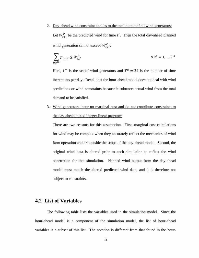
61  

2. Day-ahead wind constraint applies to the total output of all wind generators:

Let , be the predicted wind for time . Then the total day-ahead planned

wind generation cannot exceed , :

, ,

∈, ∀ 1, … ,

Here, is the set of wind generators and 24 is the number of time

increments per day. Recall that the hour-ahead model does not deal with wind

predictions or wind constraints because it subtracts actual wind from the total

demand to be satisfied.

3. Wind generators incur no marginal cost and do not contribute constraints to

the day-ahead mixed integer linear program:

There are two reasons for this assumption. First, marginal cost calculations

for wind may be complex when they accurately reflect the mechanics of wind

farm operation and are outside the scope of the day-ahead model. Second, the

original wind data is altered prior to each simulation to reflect the wind

penetration for that simulation. Planned wind output from the day-ahead

model must match the altered predicted wind data, and it is therefore not

subject to constraints.

4.2 List of Variables

The following table lists the variables used in the simulation model. Since the

hour-ahead model is a component of the simulation model, the list of hour-ahead

variables is a subset of this list. The notation is different from that found in the hour-

62  

ahead model to account for the difference between the day-ahead and hour-ahead models.

Matrix notation is used through the bolding of variables, and time indices begin at zero.

N.B.: Generator indices also begin at zero in the simulation model (instead of one

in the hour-ahead model), but this difference is less crucial because the model usually

refers to generators as a set rather than as individuals.

In addition, the decision variable notation used in the hour-ahead model is

clarified. The expression , , is defined in the hour-ahead model as the information or

decision regarding generator that is known or made at time and is actionable or

executed at time . In the simulation, time is measured by a combination of days,

hours, and sub-hourly increments, but it is possible to express time solely in hours or

solely in sub-hourly increments using parallel time notation. Let

,

where 24 is the number of time increments per day and ,

indicate the 1 hour of the 1 day of the simulation. Then , is the

cumulative , 1 hour of the simulation. For example, 0,0 0 is the first

hour of simulation. Similarly, let

, , ,

where 12 is the number of time increments per hour and indicates the

1 increment of the 1 hour of the 1 day of the simulation. Then

, , is the cumulative , , 1 increment of the simulation.

This notation clarifies the notation found in the previous chapter. The hour-ahead

variable , , , , , , , is the information or decision regarding generator that

63  

is known or made by the hour-ahead model during the cumulative hour , and

is actionable or implemented at the cumulative time increment , , , i.e.

the 1 sub-hourly increment of cumulative hour , .

Table 4‐1: List of Variables for Simulation Model 

Variable Definition Decision Variables

  Matrix  of  “warming  up/not  warming  up”  status indicator  variables  scheduled  by  the  day‐ahead model  on  day  ;  element  ,   is  generator  ’s indicator for hour   of day   

 ,   Matrix  of  “begin  warming  up/do  not  begin 

warming up”  indicator variables  scheduled by  the day‐ahead  model  on  day  ;  element  ,   is generator  ’s indicator for hour   of day   

  Matrix of “is online/is not online” status  indicator variables  scheduled  by  the  day‐ahead  model  on day  ; element  ,   is generator  ’s  indicator for hour   of day   

 ,   Matrix  of  “go  online/do  not  go  online”  indicator 

variables  scheduled  by  the  day‐ahead  model  on day  ; element  ,   is generator  ’s  indicator for hour   of day   

 ,  Matrix  of  “turn  off/do  not  turn  off”  indicator 

variables  scheduled  by  the  day‐ahead  model  on day  ; element  ,   is generator  ’s  indicator for hour   of day   

   Matrix of committed generation scheduled by the 

day‐ahead  model  on  day  ;  element  ,   is generator  ’s output during hour   of day   

  Matrix  of  slack  variables  representing  power shortages caused by  the day‐ahead model on day ; element    is  the  total amount  for hour   of 

day    

64  

,   Matrix  of  “warming  up/not  warming  up”  status indicator  variables  scheduled  by  the  hour‐ahead model  on  hour    of  day  ;  element  ,   is  fast generator  ’s  indicator  for sub‐hourly  increment   during that hour 

,,   Matrix  of  “begin  warming  up/do  not  begin 

warming up”  indicator variables  scheduled by  the hour‐ahead model  on  hour    of  day  ;  element ,   is  fast generator  ’s  indicator  for  sub‐hourly 

increment   during that hour  

,   Matrix of “is online/is not online”  status indicator variables  scheduled  by  the  hour‐ahead model  on hour   of day  ; element  ,  is fast generator  ’s indicator  for  sub‐hourly  increment    during  that hour 

,,   Matrix  of  “go  online/do  not  go  online”  indicator 

variables  scheduled  by  the  hour‐ahead model  on hour   of day  ; element  ,  is fast generator  ’s indicator  for  sub‐hourly  increment    during  that hour 

,,  Matrix  of  “turn  off/do  not  turn  off”  indicator 

variables  scheduled  by  the  hour‐ahead model  on hour   of day  ; element  ,  is fast generator  ’s indicator  for  sub‐hourly  increment    during  that hour 

,   Matrix of actual generation variables scheduled by the hour‐ahead model on hour   of day  ; element ,   is  fast  generator  ’s  actual  generation  for 

sub‐hourly increment   during that hour  

,   Matrix  of  slack  variables  representing  power shortages scheduled by  the hour‐ahead model on hour   of day  ; element    is  the  total amount for sub‐hourly increment   during that hour 

 Simulation Parameters

Number of days used in the simulation; set to 20 

65  

Number  of  time  increments  per  day  used  in  the simulation; set to 24 

  Number of  time  increments per hour used  in  the 

simulation; set to 12  

  Wind penetration (%)  

, ,   Penalty $

  for  power  shortage  during 

increment   of hour   of day      Simulation Data Components

Set of all generators  

Set  of  all  fast  generators;  planned  by  the  day‐ahead model and  rescheduled by  the hour‐ahead model 

  Set  of  all  slow  generators;  planned  by  the  day‐

ahead model and implemented exactly  

  Set  of  all  wind  generators;  planned  by  the  day‐ahead model and implemented according to actual wind by the hour‐ahead model 

   Matrix of predicted wind values; element  ,  –  

alternatively, element  ,  –  is the predicted wind value (MW) for hour   of day   

   Matrix  of  actual  wind  values;  element  ,   –  

alternatively,  element  ,   –  is  the  actual wind value (MW) for hour   of day   

   Matrix of predicted total demand values; element 

,   is  the  predicted  total  demand  value  (MW) for hour   of day   

   Matrix  of  actual  total  demand  values;  element 

,   is  the  actual  total demand  value  (MW)  for hour   of day   

66  

  Matrix of generator parameters  for all generators ∈   

, ,,  Fuel  cost 

$  of  slow  generator  ∈   during 

hour   of day    

, , ,,  Fuel  cost 

$  of  fast  generator  ∈   during 

increment   of hour   of day      Exogenous Variables  

,   Vector of  simulated  sub‐hourly wind values  taken to be actual values during hour   of day    

,   Vector  of  simulated  sub‐hourly  total  demand values  taken  to be actual values during hour   of day    

   Transition Variables  

  Vector of  end‐of‐day  variables  required  for  inter‐day transition  in the day‐ahead model from day   to  1 

,   Vector of hour‐ahead transition variables required for  inter‐hour  transition  in  the hour‐ahead model from cumulative hour  ,  to  , 1 

,   Total slow generation (MW) that is planned by the day‐ahead  model  for  hour    of  day    and  is implemented  by  the  hour‐ahead model  for  each increment of that hour 

, Vector of sub‐hourly demand values that must be satisfied  by  fast  generators  only;  is  input  to  the hour‐ahead model  and  excludes  slow  generation and actual wind power 

, , Set  of  all  sub‐hourly  increments    such  that  the instantaneous indicator variable  , , , , ,  is 1 

in hour   of day  ; used to modify the day‐ahead solution with the hour‐ahead solution 

67  

, ,  Set  of  all  sub‐hourly  increments    such  that  the 

instantaneous indicator variable  , , , , ,  is 1 

in hour   of day    

, ,   Set  of  all  sub‐hourly  increments    such  that  the instantaneous  indicator  variable  , , , , ,   is 

1 in hour   of day    

, ,  The latest time increment, if it exists, during which the instantaneous indicator variable  , , , , ,  

is 1  in hour   of day  ; used  to modify  the day‐ahead solution with the hour‐ahead solution 

, ,  The latest time increment, if it exists, during which 

the instantaneous indicator variable  , , , , ,  

is 1 in hour   of day    

, ,   The latest time increment, if it exists, during which the  instantaneous  indicator  variable 

, , , , ,  is 1 in hour   of day   

, ,   The latest time increment, if it exists, during which any of the three  instantaneous  indicator variables 

, , , , , , , , , , , , , , , , ,   is 

1 in hour   of day    

4.3 Model

The simulation model illustrates the interaction of the day-ahead model and the

hour-ahead model to create a multi-day simulation of power generation. For the day-

ahead model, time is measured in both days and hours: day ∈ 0, 1 and hour

∈ 0, 1 . For the hour-ahead model, time is further subdivided into smaller time

intervals: sub-hourly increment ∈ 0, 1 . Each time index begins at zero and ends

68  

at one less than its corresponding upper limit. Hence, days range from 0 to 19, inclusive;

hours range from 0 to 23, inclusive; increments range from 0 to 11, inclusive.

4.3.1 State Variable

The state variable at day , hour is written as follows:

, , ,

where is the state variable for the day-ahead model for day and , is the

state variable for the hour-ahead model for day , hour .

The details of the day-ahead state variable are beyond the scope of this work

and can be found in Kevin Kim’s senior thesis. It suffices to write:

Χ , , , ,

In other words, the implementation of the day-ahead algorithm Χ , takes in

the day-ahead state variable and returns seven two-dimensional matrices, each of size

| | 24 | | (except for , which is size 24 1), where is the set of all

generators used in the simulation. Each policy defines an implementation of the day-

ahead model. For convenience, let Χ be a particular implementation.

These matrices contain the mixed integer linear programming solution to the day-

ahead problem. For example, is the slack variable for hour of day , and

, is generator ’s planned “online/not online” status for hour of day .

The hour-ahead state variable , , on the other hand, is defined in the hour-ahead

model of the previous chapter using time notation. Recall that it is defined as:

, , , , , , , , , , , , , , ,

69  

There is a conceptual difference between the , time indexing, which is used

in the simulation, and the time indexing, which is used in the hour-ahead model, where

∈ 1, . A method is needed to combine these two approaches. Define | as the

state variable for cumulative time increment that is computed at time , ∈ 1, of

the current hour. Then measures cumulative time in the simulation model, and

measures time in the hour-ahead model. The state variable can be expressed as:

, , , |

This expression is evaluated at time in the hour-ahead model (recall that the

hour-ahead model indexes time starting from one). It is also clarified that for the

purposes of the simulation, the parameters , , , , , , , ,

, , , , , , and , are fully defined only at cumulative time

increment , , 1 , or time increment 1 of cumulative hour , . In the

hour-ahead model, they are defined for all time increments because of the iterative

method through which they are calculated by the hour-ahead transition functions.

4.3.2 Decision Variables

The decision variables , consist of both the day-ahead decision variables

and the hour-ahead decision variables , , which are defined as follows:

, , , : day-ahead augmented matrix for day

decision variables

, , ,, ,

, , ,, , , : hour-ahead augmented matrix

for day , hour decision variables

Recall that they are obtained from decision functions that depend on policy :

70  

Χ ,

, Χ ,,

The decision variables of the simulation model, therefore, can be written as the

following:

, , ,

4.3.3 Exogenous Information

The exogenous information has two components. The first is , , the

simulated actual wind power in MW for day , hour . This is a 1 vector, where

, is the simulated actual wind power for sub-hourly increment . This vector is

exogenous to the day-ahead and hour-ahead models. The actual wind power data is

given in hourly increments per day, but the hour-ahead model requires sub-hourly values.

Hence sub-hourly values are simulated using a function Ω that depends on the policy

(e.g. linear interpolation or Brownian bridge simulation):

, Ω , ,

The second piece of exogenous information is , , the simulated total load for

day , hour . This is a 1 vector, where , is the simulated total demand that

must be satisfied for sub-hourly increment . This vector is exogenous to the day-ahead

and hour-ahead models. The actual demand data is given in hourly increments per

day, but the hour-ahead model requires sub-hourly values. Hence sub-hourly values are

simulated using a policy -dependent function Λ :

, Λ , ,

71  

The method of linear interpolation is used to obtain all sub-hourly demand values

for the simulations. Let be the difference between current hourly demand and the

next hourly demand split into equal sub-hourly intervals.

, 1 ,

Then the actual demand is computed as follows:

, , ∀ ∈ 0, 1

Linear interpolation is used for all hours except the very last hour of the very last

day of simulation. The end value of the interpolation , 1 does not appear in

the same vector as the beginning value , to avoid repeating values. Instead it

appears as the beginning value of the vector of the next hour. Linear interpolation is also

used to generate sub-hourly wind values for all simulations unless otherwise noted.

4.3.4 Transition Functions

These functions incorporate the modifications made by the hour-ahead model to

the day-ahead generation schedule. They are necessary for the day-ahead model to

compute the end-of-day transition variables, which are needed to make the new day-

ahead schedule for the next day. Let and be the current day and hour indices,

respectively, and let ′ and ′ be the day and hour indices of the next hour. Then

is the transition function of the simulation model such that:

, , , Χ , Χ ,, , ,

In particular, the hour-ahead model may change the statuses and output of the fast

generators, so the transition functions must transmit this information to the day-ahead

72  

model. To do so, it is necessary to calculate the current slow generation planned by the

day-ahead model:

, ,∈

The hour-ahead model implements the schedule for slow generators because slow

generators generally cannot complete a full off – warm-up – online cycle within the hour.

Next, define the total load that must be satisfied by the fast generators only:

, , , ,

This is a 1 vector of demands in sub-hourly increments. Then the output of

the hour-ahead model Χ , can be written as:

Χ ,, , , ,

, ,, ,

, , ,, , ,

Again, it is convenient to write Χ for a particular implementation of the hour-

ahead model. Each of the output matrices is of size | | except for , , which is a

1 vector. For example, , , denotes gas generator ’s “warming up/not

warming up” status during sub-hourly increment of hour of day .

Let be a mapping of indices such that index in ⊂ maps to index

in . After each hour of the simulation, the transition functions require that the

gas generator statuses in the day-ahead solution matrices be updated with the newly

determined hour-ahead values:

, , 1, , ∀ ∈

, , 1, , ∀ ∈

, , 1, , ∀ ∈

73  

The “online/not online” status, the “warming up/not warming up” status, and the

output of each gas generator at each hour, from the day-ahead model’s point of view, are

simply their respective values at the last (i.e. 1 11) sub-hourly increment of

the hour, from the hour-ahead model’s point of view. The reason is that these three

variables are continuous, so whichever values they take at the end of the hour should be

used by the day-ahead model to calculate the generation schedule for the following day.

The values that they take within the hour are irrelevant to the day-ahead model.

The transition functions for the instantaneous decision variables, however, are

different because the most recent time those were nonzero may not have occurred during

increment 11. Define the following sets of instantaneous hit times:

, , ∈ : ∈ 0, 1 , ,, , 1 , ∀ ∈

, , ∈ : ∈ 0, 1 , ,, , 1 , ∀ ∈

, , ∈ : ∈ 0, 1 , ,, , 1 , ∀ ∈

These sets contain all sub-hourly increments within hour during which the

instantaneous decision variables are 1. Define the following transition times:

, ,max , , , , ∅∞

, ∀ ∈

, ,max , , , , ∅∞

, ∀ ∈

, ,max , , , , ∅∞

, ∀ ∈

, , max , , , , , , , , , 1 , ∀ ∈

74  

The first three transition times are the latest sub-hourly increments of hour

during which each instantaneous variable was 1 (if the instantaneous variable was 0

during the entire hour, then the value is set to ∞). Transition time , , is the latest

sub-hourly increment of hour where any of the three instantaneous decision variables

was 1 (otherwise its value is 1). Then the transition functions are:

, , 1 , , , ,

0 , ∀ ∈

, , 1 , , , ,

0 , ∀ ∈

, , 1 , , , ,

0 , ∀ ∈

At any given hour , therefore, at most one of the instantaneous decision

variables stored in the day-ahead solution has value 1. These functions give the day-

ahead model the most up-to-date information to continue the simulation for the next day.

4.3.5 Objective Function

The objective function of the simulation model consists of minimizing the

expected sum of the day-ahead slow generation costs and the hour-ahead fast generation

costs and shortage penalties. The minimization is done over policies associated with

tunable parameters. The decision variable vectors , , , and , are dependent on

through the implementations of the day-ahead and hour-ahead models Χ , and Χ , ,

respectively. Using , , ,, , and ,

, to make the policy dependency explicit, the

objective function can be represented as follows:

75  

min , ,, , ,

∈ ,∈ ,∈

, , ,,

,, , , ,

∈ ,∈ ,∈ ,∈

,, ,

For the simulation model, costs for slow generators are ideally given per hour,

whereas costs for fast generators and shortage penalties are ideally given per sub-hourly

increment. Due to lack of data, however, these parameters may only be given per day.

In addition, the total cost for each simulation analyzed in the results does not

include the costs from day 0 because of the time it takes for slow generators to get up to

speed. For consistency, cost of fast generation and shortage penalties from day 0 are also

not included.

76  

Chapter V

5 Simulation Data

The simulation data are obtained from PJM and can be split into three categories:

generator data, demand data, and wind data. Table 5-1 displays the distribution of

generators used in the simulations.

Table 5‐1: Generator Distribution in Simulations 

Type of Generator Number Used in Simulation

Steam 384

Nuclear 31

Hydro 77

Combustion Turbine 482

Diesel 39

Landfill 28

Wind 12

The set of fast generators that is scheduled by the hour-ahead model contains

605 generators. It includes all of the combustion turbine, diesel, and landfill generators

as well as the steam generators that are listed as having no minimum warm-up time.

One weakness of the PJM generator data is that generator costs are bid costs: the

cost each generator claims to incur when submitting bids to PJM. The bid cost is not

necessarily the generator’s actual cost of operation; for example, operators of coal

generators with high fixed costs may bid zero cost when their generators are already

online because selling output at any price would be more profitable than turning off the

generator. Despite this inconsistency, the use of bid costs does not present a significant

77  

problem because the total generation cost calculated at the end of the simulation is only

an indicator of the simulation’s performance and should not be taken as a precise value.

5.1 Generator Data

PJM provides data on many parameters for each generator in its system, a few of

which are used in the simulation. For each generator , the necessary parameters are

, , , , , Δ , Δ , , . Each parameter is also listed

below in uppercase and parentheses as it is categorized in the PJM data.

The minimum capacity is set to the economic minimum watts

(ECONOMIC_MIN), given in MW. The maximum capacity is set to the economic

maximum watts (ECONOMIC_MAX), given in MW. Values in MW do not need to be

converted in the hour-ahead model because MW is a unit of power.

The minimum online time is set to the minimum run time

(MIN_RUN_TIME). The minimum off time is set to the minimum down time

(MIN_DOWN_TIME). The minimum warm-up time is set to the cold start-up

time (COLD_STARTUP_TIME). PJM gives these three minimum times in hours, so

they must be converted to number of five minute increments by multiplying by 12.

In addition, each minimum time has a floor of one due to the implementation of the hour-

ahead model.

The ramp-up rate Δ is set to the ramp rate (RAMP_RATE). The ramp-down

rate Δ is set to negative the value of the ramp rate. PJM gives these rates in , so

they must be converted to

by dividing by 12.

78  

The fuel cost , is given by a mean value of the cost curve as a function of the

demand bids. In this implementation, therefore, it is not a function of time and can be

written as . The mean value is calculated from the minimum capacity lower bound

to the maximum capacity upper bound. Let be generator ’s cost in dollars given

the generator’s bid at time . Then the fuel cost is defined as follows:

The integral is discretized and approximated with the trapezoidal rule by using

price (PRICE1, PRICE2, PRICE3, etc.) and megawatt (MW1, MW2, MW3, etc.) values.

Within the mixed integer linear programming implementation, the shortage

penalty is fixed for all time periods at $

. When calculating the total

simulation cost, however, the value is fixed for all time periods at $

. A

larger value is used in the linear program to force demands to be satisfied whenever

possible.

5.2 Demand Data

The demand data used is 2009 actual and predicted demand obtained from PJM.

The dataset contains hourly values for predicted and actual demand for each day in 2009.

For these 20 day simulations, the first day of each simulation is January 1, 2009.

Figure 5-1 is a graph of total actual demand versus total predicted demand during

the 20 day simulation. Peak actual demand values tend to be under-predicted. As a

79  

result, the hour-ahead model must reschedule the day-ahead solution to satisfy this

demand.

Figure 5‐1: Actual Demand vs. Predicted Demand

Figure 5-2 is a zoomed-in version of the same graph for hours 13 through 20 (day

0) of the data. Predicted demand is a step function because only hourly values are given;

actual demand is not because sub-hourly values are simulated using linear interpolation.

Figure 5‐2: Actual Demand vs. Predicted Demand (Zoomed)

0

20000

40000

60000

80000

100000

120000

Dem

and

(M

W)

Day

Actual Demand vs. Predicted Demand

Actual Demand

Predicted Demand

65000

70000

75000

80000

85000

90000

95000

13 14 15 16 17 18 19 20

Dem

and

(M

W)

Hour

Actual Demand vs. Predicted Demand

Actual Demand

Predicted Demand

80  

5.3 Wind Data

The simulation uses PJM’s actual wind data for each hour of each day in 2009.

The predicted wind value for a given day and hour is the 7-day previous actual wind

value measured at the same hour. For example, the predicted wind value for hour 15 on

January 10, 2009 is the actual wind value for hour 15 on January 3, 2009. All wind

values are initially scaled to simulate the effect of having more wind power available to

the system.

The wind penetration is a simulation parameter that expresses the ratio of total

actual wind power to total actual power. The parameter depends on policy but can be

written as for convenience. Let be the matrix of reserve requirements calculated by

the day-ahead model, where , is the reserve requirement for hour of day . Then

is calculated as follows:

∑ ∑ ∑ ,

∑ ∑ ∑ , , ∑ ∑ ∑ ∑ , ,∈ ∑ ∑ ∑ ∑ ,, ,∈

The summations are carried out over all days, all hours, and all sub-hourly

increments of the simulation. The reserve requirement is incorporated because the wind

penetration includes the day-ahead model’s perspective. Different levels of wind

penetration are tested to analyze how well the system can integrate wind power. Since

can be calculated only after the simulation terminates, however, several simulations are

run to adjust the wind data to the appropriate scale so that the final wind penetration

parameter matches the intended wind penetration of the simulation.

81  

Figure 5-3 is a graph of actual wind versus predicted wind at the 5% level during

the 20 day simulation. Wind is much more volatile than demand: the difference between

actual and predicted wind is much larger than that of demand.

Figure 5‐3: Actual Wind vs. Predicted Wind

Figure 5-4 is a zoomed-in version of the same graph for hours 13 through 20 (day

0) of the data. Again, the hourly predicted wind is a step function, whereas sub-hourly

actual wind values are generated using linear interpolation.

Figure 5‐4: Actual Wind vs. Predicted Wind (Zoomed)

0

2000

4000

6000

8000

10000

12000

Win

d P

ow

er (

MW

)

Day

Actual Wind vs. Predicted Wind

Actual Wind

Predicted Wind

0

1000

2000

3000

4000

5000

6000

7000

8000

13 14 15 16 17 18 19 20

Win

d P

ow

er (

MW

)

Hour

Actual Wind vs. Predicted Wind

Actual Wind

Predicted Wind

82  

Chapter VI

6 Results and Analysis

For each of the following cases, a 20 day simulation is run using linearly

interpolated wind and demand values. Three levels of wind penetration are tested:

5.2%, 20.4%, and 40.0%. These simulations reveal substantial

differences in the distribution of slow versus fast power, the number of shortages and

overages, the distribution of total cost, and generator activity.

N.B.: The analyzed percentage differences and costs exclude day 0 of the

simulation because it takes time for the slow generators to get up to speed.

6.1 5.2% Wind

The first simulation is run for 20 days with 5.2% wind penetration. The total cost

of simulation is $3.96 10 . The total cost is computed by summing generation costs

and shortage penalties at each sub-hourly increment, excluding day 0. It is not directly

comparable, therefore, to the total cost of a simulation that does not implement the hour-

ahead model in sub-hourly increments.

6.1.1 The Advantages of Hour-Ahead Rescheduling

Figure 6-1 shows the planned power versus the predicted demand for the 20 day

simulation. The two functions are step-like because they are computed at hourly intervals

and are held constant throughout each hour (for the purposes of the simulation). The total

83  

planned power starts from a value close to zero and takes 21 hours to first reach the

predicted demand level. The reason is that generators begin from a cold start on the

initial day. The initial value is not zero because there is still planned wind power during

the first hour of the first day, and wind power does not begin from a cold start.

Figure 6‐1: Planned Power vs. Predicted Demand (5.2%) 

The total planned power is the solution planned by the day-ahead model and

includes planned power from slow generators, planned power from fast generators, and

predicted wind power. The planned power from the slow generators is implemented

according to the day-ahead solution and becomes part of actual power. The planned fast

power from the hour-ahead model, on the other hand, is rescheduled by the hour-ahead

model. Similarly, the predicted wind power is eventually replaced by the actual wind

power simulated within each hour.

Even without the readjustment of the planned power, however, it still does not

completely satisfy the predicted demand. Figure 6-2 is the previous graph zoomed in on

0

20000

40000

60000

80000

100000

120000

Po

wer

(M

W)

Day

Planned Power vs. Predicted Demand

Total Planned Power

Predicted Demand

84  

hours 323 through 330 (day 13) of the simulation. There is not enough total planned

power to satisfy predicted demand during this interval. If implemented, the shortage of

the day-ahead solution as measured in sub-hourly increments would total approximately

4 million MW. Combined with the fact that the actual demand and wind differ from their

predicted values, it becomes clear that, despite serving as a good approximation, the day-

ahead solution is not an adequate implementable schedule.

Figure 6‐2: Planned Power vs. Predicted Demand (Zoomed, 5.2%) 

If the planned power is not updated and is implemented to satisfy actual demand,

the total simulation shortage is about 18 million MW. This constitutes a 350% increase

compared to the day-ahead schedule applied to predicted demand. Figure 6-3 shows that

the day-ahead schedule often misses the peak values of the actual demand. These

shortages cause significant penalties and increase the total cost of simulation. The day-

ahead schedule, therefore, should be modified on a smaller time scale to reduce the

difference between planned power and actual demand.

95000

98000

101000

104000

107000

110000

113000

Po

wer

(M

W)

Hour

Planned Power vs. Predicted Demand

Total Planned Power

Predicted Demand

85  

Figure 6‐3: Planned Power vs. Actual Demand (5.2%) 

Taking into account actual wind values and the implemented day-ahead slow

generation, the hour-ahead model adjusts the fast generator output in sub-hourly

increments. Figure 6-4 shows the result, in which total shortage is reduced over 90% to

about 328000 MW.

Figure 6‐4: Actual Power vs. Actual Demand (5.2%) 

0

20000

40000

60000

80000

100000

120000

140000

Po

wer

(M

W)

Day

Planned Power vs. Actual Demand

Total Planned Power

Actual Demand

0

20000

40000

60000

80000

100000

120000

140000

Po

wer

(M

W)

Day

Actual Power vs. Actual Demand

Total Actual Power

Actual Demand

86  

Figure 6-5 is a graph of actual power versus actual demand zoomed in on hours

323 to 330 (day 13) of the simulation. The actual power almost exactly matches the

actual demand, differing in only three increments on this interval (two of these

differences are easily visible in the graph). In the entire 20 day simulation, in fact, the

actual power exactly matches the actual demand in 4630 out of the 5760 total five minute

increments, or approximately 80% of the time.

Figure 6‐5: Actual Power vs. Actual Demand (Zoomed, 5.2%) 

6.1.2 Explanation of Shortages

In the 5.2% simulation, the time increments during which actual power does not

exactly match actual demand are often the first increment of the hour. Not including day

0 of the simulation, 177 shortages occur at time increment 0, totaling about 223000 MW.

In contrast, only 87 potential shortages occur on all other time increments 1 through 11

inclusive, totaling about 105000 MW: less than half of the former amount. This

observation is explained by a limitation of this hour-ahead model implementation.

97000

99000

101000

103000

105000

107000

109000

Po

wer

(M

W)

Hour

Actual Power vs. Actual Demand

Total Actual Power

Actual Demand

87  

Consider the actual power output during the last 30 minutes of hour 430 and the first 30

minutes of hour 431 (day 17 of the simulation) in Figure 6-6. Time increment 0

corresponds to the first five minutes of hour 431, which incurs a shortage of 3989 MW

shown on the primary axis. The shortage occurs as a result of the horizon of the hour-

ahead model.

Figure 6‐6: Explanation of Shortage (5.2%) 

The hour-ahead model solves a mixed integer linear program with a one hour

horizon, meaning that all 12 of its solutions – one per five minute increment – are

implemented. In this implementation, the hour-ahead model cannot foresee the planned

slow generation of the next hour, nor could the day-ahead model have foreseen the

ending fast generation of the current hour when generating the day-ahead schedule. If the

difference in planned slow generation between this hour and the next hour is not great, or

if the difference between actual fast generation between this hour and the planned fast

generation of the next hour is not great, then no major problems arise. If, on the other

hand, a significant discrepancy in the aforementioned values exists, shortages may occur.

68000

69000

70000

71000

72000

73000

74000

75000

0

2000

4000

6000

8000

10000

12000

14000

6 7 8 9 10 11 0 1 2 3 4 5

Slow Power (M

W)

Fas

t P

ow

er (

MW

)

Time Increment

Explanation of Shortage during Hour 431

Shortage

Fast Power

Planned Fast Power

Slow Power

88  

Hour 431 of the simulation, illustrated in the above figure, is an example of the

latter case. The planned slow power decreases by a significant amount between hours

430 and 431, but the day-ahead schedule had anticipated that fast power (“planned fast

power”) was at a higher value than it actually was (“fast power”) at the start of hour 431,

which would have cushioned the significant decrease in planned slow power. The hour-

ahead model, however, is able to satisfy the actual demand with lower generation and, as

a result, decreases the fast power from time increment 6 through 11 (in this

implementation, the hour-ahead model cannot change the amount of slow power). When

hour 431 arrives, there is not enough power to satisfy actual demand because both the

slow power and fast power are too low, hence the shortage at time increment 0. It takes

one time increment for the hour-ahead model to incorporate this information and ramp up

fast power accordingly, and the shortage disappears by time increment 1.

The difference between actual and predicted wind is an indirect cause of this

phenomenon: large predicted wind power causes the day-ahead model to schedule low

amounts of slow power. If actual wind power is much smaller during that interval, the

fast power required to satisfy actual demand is much larger, leading to shortages.

A potential fix for this limitation is increasing the horizon of the hour-ahead

model by five minutes but not implementing the solution of the last time increment.

Another potential method is to allow the hour-ahead model to modify the planned slow

generation by ramping up or down the slow generators that are already online.

6.1.3 Distribution of Generated Power

Figure 6-7 highlights the difference in magnitude between the different sources of

power. The actual fast power tends to exceed the planned fast power, but each is on

89  

average several multiples lower than the slow power. This result makes sense because

slow power is used to satisfy the baseload, which accounts for the majority of the power

supplied. Fast power, on the other hand, is used to satisfy the peakload, which is more

volatile but smaller in magnitude.

Figure 6‐7: Slow Power vs. Fast Power (5.2%) 

6.1.4 Percentage Difference in Overages and Shortages

Figure 6-8 displays the percentage difference between actual power and actual

demand. Negative values indicate that curtailments in actual demand are necessary to

prevent shortages. The majority of the largest shortages occur in day 0, when the

generators are getting up to speed. Otherwise, there are periodic overages and shortages

throughout the simulation.

0

15000

30000

45000

60000

75000

90000

Po

wer

(M

W)

Day

Slow Power vs. Fast Power

Slow Power

Fast Power

Planned Fast Power

90  

Figure 6‐8: Percentage Difference (5.2%) 

Percentage difference omitting day 0 of the simulation is graphed with actual

wind in Figure 6-9. With the exception of day 7, most of the shortages coincide with low

amounts of actual wind.

Figure 6‐9: Percentage Difference vs. Actual Wind (5.2%) 

‐100

‐80

‐60

‐40

‐20

0

20

% D

iffe

ren

ce

Day

Percentage Difference between Actual Power and Demand

0

2500

5000

7500

10000

‐8

‐4

0

4

8

Win

d P

ow

er (

MW

)

% D

iffe

ren

ce

Day

Percentage Difference vs. Actual Wind

% Difference

Actual Wind

91  

6.1.5 Average and Instantaneous Generator Status

Figure 6-10 displays the number of fast generators that are warming up, online,

and off at any given time. An average 13 generators are warming up at any given time,

which is much lower than the average number at any given time that are online or off

(269 and 323, respectively). Note that the number of online generators cycles rapidly

between high and low values, reflecting their ability to satisfy peakload due to their short

minimum warm-up times. Despite the fact that most of the fast generators have

minimum warm-up and online times shorter than one hour, the large quantity of fast

generators seems to eliminate the need of rapid cycling on an hourly scale.

Figure 6‐10: Distribution of Generator Status (5.2%) 

It is helpful to examine a typical generator’s continuous state throughout the

entire simulation and draw conclusions about how it operates. Figure 6-11 depicts the

status of generator 28 for each sub-hourly time increment of the simulation. On the y-

0

100

200

300

400

500

600

#

Day

Number of Generators by Status

Warming Up

Online

Off

92  

axis, 1 indicates that the generator is online, 0.5 indicates that the generator is warming

up, and 0 indicates that the generator is off.

The generator immediately goes to the warming up state at the beginning of the

simulation and goes online and turns off according to the hour-ahead schedule. Although

the generator spends the majority of its time online, it does rapidly cycle between the off,

warming up, and online states many times during the simulation. This characteristic may

be due to the fact that this implementation of the hour-ahead model does not factor in

warm-up costs, so generators are not penalized for frequently turning off and starting

back on. Note also that the generator does not spend long consecutive time increments in

the off state, suggesting that this generator is used frequently in the simulation.

Figure 6‐11: Status of Generator 28 (5.2%) 

0

0.5

1

Sta

tus

Day

Status of Generator 28

93  

6.2 5.3% Wind with Brownian Bridge Simulation

The second simulation is run for 20 days with 5.3% wind penetration and linear

interpolation of actual demand values. The sub-hourly actual wind values, however, are

simulated with a Brownian bridge. The purpose of this test is to simulate the volatile

characteristic of actual wind values more accurately and assess its effect on the

simulation. Linearly interpolating between hourly wind values makes the intra-hour

values much less volatile than they are in reality. Although the hour-ahead model

nonetheless treats these sub-hourly values as true values, the resulting volatility poses a

challenge for the hour-ahead model because the demand that must be satisfied by fast

generators becomes more volatile.

Introducing the volatility through the sub-hourly wind values is more realistic

than introducing it through the sub-hourly demand values because demand forecasts, in

practice, are much more accurate than wind forecasts. It is not necessary, furthermore, to

introduce noise in both components because this test is merely a heuristic for observing

what would happen as a result of increased volatility. In this simulation, therefore, the

sub-hourly actual demand values are still generated using linear interpolation.

6.2.1 Methodology

Let be the hourly variance used for simulating the sub-hourly actual wind

values. Let … be i.i.d random variables drawn from a 0,1 distribution: each

is a standard normal variable with mean 0 and variance 1. Then , is a 1 simulated

Brownian motion with the first element fixed at , .

94  

,

, 0

, 1√

, ∀ ∈ 0, 1

Define as the initial adjustment to pin the upper endpoint.

, 1 , 1

N.B.: During the last hour of the last day of simulation, a different value is

substituted for , 1 since has size .

Let , be the vector modified by the initial adjustment. Then , is an

effective simulated Brownian motion fixed between , and , 1 ,

except the latter value does not appear as the last element of this wind vector but rather as

the first element of the wind vector for the next hour. This convention is used to avoid

repeating , 1 .

,, 0

, , ∀ ∈ 0, 1

Finally, wind power cannot be negative. Define the secondary adjustment as

the minimum of all negative values in , .

, ∈ ∈ 1, 1 , , 0

0 , ∅

min ,

The secondary adjustment is zero if , has no negative values. All of the

simulated values are adjusted so that the minimum is not negative. Recall that , is the

vector of simulated actual wind values, which is an input to the hour-ahead model.

,, 0

, , ∀ ∈ 0, 1

95  

This method of generating , is different from simulating a Brownian bridge for

several reasons, primarily that , is not pinned on both endpoints of the same vector

and that simulated values are adjusted so that the smallest value is zero. Note that the

latter is not unreasonable in the context of this simulation because actual wind power can

be zero. Nevertheless, this method is referred to as Brownian bridge simulation for

convenience.

The variance used for this simulation is the average of the hourly wind variance

for each day over all days in the simulation. Let … be the sample variance of

the members in the sets 0, … 1, , respectively. In other

words, , is the set of 24 wind values for day , and is the sample

variance of that set. Then the variance used for Brownian bridge simulation is:

1

Although a -day rolling average of hourly variance would more closely capture

the correlated nature of wind, this approach is preferred for its simplicity. More

sophisticated algorithms for intra-hourly wind simulation are not necessary because the

main purpose of this subsection is to assess the effect of larger wind volatility on

simulation performance.

6.2.2 Results

The actual wind power from the Brownian bridge simulation is much more

volatile than the original wind power, as shown in Figure 6-12. Although the average

wind power per time increment increases 1.2%, the variance increases 14.3%. The

96  

original wind penetration is 5.2%, whereas the new wind penetration increases to 5.3%

due to a larger proportion of wind power in the system. For 32 time increments in the

simulation, the actual wind power is zero; this number comprises 0.6% of the total time

increments in the simulation.

Figure 6‐12: Actual Wind with Brownian Bridge (5.3%)

The cost of the 5.3% Brownian bridge simulation is $4.19 10 , which is 5.8%

more expensive than the 5.2% base case simulation. The increase in cost is expected

because volatile wind power makes it more difficult for the hour-ahead model to prevent

shortages. Figure 6-13 displays the percentage difference between total actual power and

total actual demand for the Brownian bridge simulation and the original simulation.

Although many time increments in the Brownian bridge case experience shortages where

none existed in the base case, there are also time increments where the base case has

shortages but the Brownian bridge case does not.

0

2000

4000

6000

8000

10000

12000

Win

d P

ow

er (

MW

)

Day

Actual Wind Power by Wind Interpolation

Brownian Bridge

Original

97  

Figure 6‐13: Percentage Difference with Brownian Bridge (5.3%)

Thus, a temporal pattern between original and new shortages is not obvious. The

Brownian bridge simulation does, however, increase the number of shortages and

overages, which is shown in Table 6-1. The total shortage and overage also increase, but

the average shortage and overage decrease. These results suggest that when wind is

volatile, it is more difficult for the hour-ahead model to commit power that exactly

matches demand, leading to more frequent – yet smaller – shortages and overages.

Indeed, the number of time increments where actual power exactly matches actual

demand decreases from 4518 to 4246 when Brownian bridge simulation is used. Note

also that the percentage increase in total shortage is over six times as large as the

percentage increase in total overage. The increased volatility of wind, therefore, affects

shortages more than overages, which increases cost.

‐9

‐6

‐3

0

3

6

% D

iffe

ren

ce

Day

Percentage Difference by Wind Interpolation

Brownian Bridge

Original

98  

Table 6‐1: Shortages and Overages with Brownian Bridge (5.3%) 

Total (excluding day 0)

5.3% Wind(Brownian Bridge)

5.2% Wind(Original)

% Change

# shortages  468 264 7.7%

Total shortage (MW) 

532000 328000 6.2%

Average shortage (MW) 

1140 1240 -8.5%

# overages  758 690 9.9%

Total overage (MW) 

164000 162000 1.0%

Average overage (MW) 

216 235 -8.0%

Table 6-2 confirms that the effect of shortages outweighs the effect of overages.

The increase in shortage penalty is 62%, which is over 50 and 100 times greater than the

increase in the cost of slow and fast generation, respectively.

Table 6‐2: Cost Distribution with Brownian Bridge (5.3%) 

Cost ($ ) (excluding day 0)

5.3% Wind(Brownian Bridge)

5.2% Wind(Original)

% Change

Slow power cost 239 238 0.6%

Fast power cost  126 125 1.1%

Shortage penalty  53 33 62%

Total cost  419 396 5.8%

Table 6-3 shows the changes in generation due to Brownian bridge simulation.

With large wind volatility, the emphasis shifts toward satisfying peakload, which leads to

an increase in total fast generation at the expense of total slow generation. Changes in

committed generation occur in 1000+ time increments for both slow and fast generation.

Volatility in actual wind power is an important part of how the hour-ahead schedule is

created, irrespective of whether actual or predicted values are used as inputs to the model.

99  

Table 6‐3: Changes in Generation with Brownian Bridge (5.3%) 

Changes in Generation (excluding day 0)

5.3% Wind(Brownian Bridge)

% change in total slow generation (10 MW) -0.26%

# time increments with increased slow generation  1668

# time increments with decreased slow generation  3084

% change in total fast generation (10 MW) 0.55%

# time increments with increased fast generation  2884

# time increments with decreased fast generation  2556

6.3 20.4% Wind

The next simulation is run for 20 days with 20.4% wind penetration. Linear

interpolation is used to generate sub-hourly wind and demand values. Since obtaining

accurate five minute predictions of wind and demand is beyond the scope of this thesis,

the use of linear interpolation suffices for the rest of these simulations.

The total cost of the 20.4% simulation is $2.91 10 , or about 26.4% cheaper

than the 5.2% simulation. Wind power is assumed to be free, so 20.4% of the total actual

power is supplied at no cost, compared to only 5.2% of the previous total power. At the

same time, however, wind penetration has not yet increased to the point where volatility

causes shortages that significantly increase total cost. Figure 6-14 compares the actual

wind for the two simulations.

100  

Figure 6‐14: Actual Wind (20.4%, 5.2%)

Figure 6-15 contrasts actual slow and actual fast power in the 20.4% and 5.2%

simulations. Both types of 20.4% power are in general smaller in magnitude because less

fast and slow power is needed. The 20.4% slow power, in addition, is more volatile. The

baseload fluctuates more because 20.4% wind is more volatile than 5.2% wind.

Furthermore, the amount of 20.4% fast power is almost zero for the time increments

where 20.4% wind and slow power are sufficient to satisfy actual demand.

Figure 6‐15: Slow Power vs. Fast Power (20.4%, 5.2%) 

0

9000

18000

27000

36000

45000

Win

d P

ow

er (

MW

)

Day

20.4% vs. 5.2% Actual Wind

20.4% Wind

5.2% Wind

0

10000

20000

30000

40000

50000

60000

70000

80000

90000

Po

wer

(M

W)

Day

Actual Power by Wind Penetration

20.4% Slow Power

20.4% Fast Power

5.2% Slow Power

5.2% Fast Power

101  

The percentage difference between actual power and actual demand again appears

to be highly correlated with the amount of available wind power, as seen in Figure 6-16.

Amounts of wind power over 16000 MW lead to overages that tend to last multiple time

increments; lower levels of wind tend to lead to brief shortages. Overages occur when

the wind and slow power exceed the actual demand. During these time increments, fast

power cannot be ramped down further (otherwise, the hour-ahead model would incur

larger costs and would not have found the optimal solution). Slow power, on the other

hand, cannot be modified by the hour-ahead model. Total generation costs may be

reduced by allowing the hour-ahead model to modify slow generation.

Figure 6‐16: Percentage Difference vs. Actual Wind (20.4%) 

Figure 6-17 compares the percentage differences between the 20.4% and 5.2%

simulations. The former has more overages (2591 versus 690) and fewer shortages (158

versus 264) due to the increased amount of available wind power.

0

8000

16000

24000

32000

40000

‐20

‐10

0

10

20

30

Wind Power (M

W)

% D

iffe

ren

ce

Day

Percentage Difference vs. Actual Wind

% Difference

20.4% Wind

102  

Figure 6‐17: Percentage Difference (20.4%, 5.2%) 

6.4 40.0% Simulation

The third simulation is run for 20 days with 40.0% wind penetration. The

resulting cost is $4.02 10 , which is larger than each of the other simulations. With

40.0% wind penetration, the magnitude of actual wind power is much larger, with a mean

of 39779 MW compared to 18800 MW (20.4% simulation) and 4736 MW (5.2%

simulation). Figure 6-18 shows that wind power is also more volatile at the larger wind

penetration, with a standard deviation of 18951 MW compared to 8957 MW and 2256

MW, respectively. Total generation costs are the largest of the three wind penetration

simulations because the wind volatility is now large enough that it causes problems for

the hour-ahead model in committing fast generation, despite the cost reductions of using

free wind.

‐20

‐10

0

10

20

30

% D

iffe

ren

ce

Day

Percentage Difference by Wind Penetration

% Difference (20.4% Wind)

% Difference (5.2% Wind)

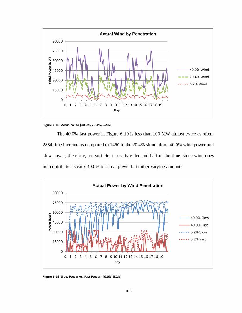
103  

Figure 6‐18: Actual Wind (40.0%, 20.4%, 5.2%) 

The 40.0% fast power in Figure 6-19 is less than 100 MW almost twice as often:

2884 time increments compared to 1460 in the 20.4% simulation. 40.0% wind power and

slow power, therefore, are sufficient to satisfy demand half of the time, since wind does

not contribute a steady 40.0% to actual power but rather varying amounts.

Figure 6‐19: Slow Power vs. Fast Power (40.0%, 5.2%) 

0

15000

30000

45000

60000

75000

90000

Win

d P

ow

er (

MW

)

Day

Actual Wind by Penetration

40.0% Wind

20.4% Wind

5.2% Wind

0

15000

30000

45000

60000

75000

90000

Po

wer

(M

W)

Day

Actual Power by Wind Penetration

40.0% Slow

40.0% Fast

5.2% Slow

5.2% Fast

104  

The overages from the 40.0% simulation dwarf those from the 20.4% and 5.2%

simulations, as seen in Figure 6-20. Although the overages are larger and more frequent,

total generation costs still decrease to $1.84 10 due to higher wind penetration.

Figure 6‐20: Percentage Difference (40.0%, 20.4%, 5.2%) 

6.5 Comparison of Wind Penetration Simulations

The three levels of wind penetration tested are 5.2%, 20.4%, and 40.0%. In

general, overages increase in frequency and magnitude as wind penetration increases,

whereas shortages display a more complex relationship due to the dip in their frequency

and magnitude at 20.4% wind. Generation costs decrease with wind penetration, whereas

shortage penalties tend to increase with wind penetration (20.4% wind is again an

exception). The average number of online generators decreases with wind penetration,

but the average number of warming-up generators is approximately constant. These

findings are summarized below in greater detail.

‐30

‐15

0

15

30

45

60

% D

iffe

ren

ce

Day

Percentage Difference by Wind Penetration

40.0%

20.4%

5.2%

105  

6.5.1 Shortages and Overages

Table 6-4 presents data on shortages and overages rounded to three significant

digits for each of the three wind penetration simulations. Although the average shortage

increases in size as wind penetration increases from 5.2% to 20.4%, shortages decrease in

frequency and total size because a higher amount of wind is available in the system. As

wind penetration increases to 40.0%, however, the hour-ahead model encounters more

difficulty coping with the higher volatility of wind, which increases the frequency, total

size, and average size of shortages.

The relationship between overages and wind penetration is more straightforward.

As wind penetration increases, the frequency, total size, and average size of overages all

increase. Furthermore, the marginal increase in total and average overage also increases.

A drawback of this implementation of the hour-ahead model is that it cannot adjust slow

power. Thus, when actual wind and slow power greatly exceed actual demand, overages

occur and power is wasted.

Table 6‐4: Shortages and Overages (5.2%, 20.4%, 40.0%) 

Total (excluding day 0) 

5.2% Wind 20.4% Wind  40.0% Wind

# shortages  264 158 445

Total shortage (MW)  328000 247000 2190000

Average shortage (MW)  1240 1560 4920

# overages  690 2591 3376

Total overage (MW)  162000 8930000 51100000

Average overage (MW)  235 3450 15100

106  

6.5.2 Cost

Table 6-5 presents cost distribution data rounded to three significant digits for the

three simulations. The total cost for the 20.4% simulation is less than that of the 5.2%

simulation due to greater wind penetration and the assumption that wind power costs

nothing. Slow power cost and fast power cost are lower because more wind is used to

satisfy actual demand. Shortage penalties also decrease due to fewer shortages. Costs

increase, however, in the 40.0% simulation. Although slow power cost and fast power

cost decrease further compared to the 20.4% simulation (due to double the wind

penetration), an increased frequency and severity of shortages causes the shortage penalty

to be more than six times as large as that of the other simulations.

It is worth noting, however, that the total cost is approximately the same for the

5.2% and 40.0% simulations (the cost of the latter represents only a 1.5% increase over

the cost of the former). Rather, only the breakdown of the costs is different: at the lower

wind penetration, almost 92% of the cost comes from generation, whereas at the higher

wind penetration, less than 46% is due to generation, with the remainder resulting from

shortage penalties.

Table 6‐5: Cost Distribution (5.2%, 20.4%, 40.0%) 

Cost ($ ) (excluding day 0)

5.2% Wind 20.4% Wind 40.0% Wind

Slow power cost 238 195 116

Fast power cost  125 71 68

Shortage penalty  33 25 219

Total cost  396 291 402

107  

6.5.3 Generator Status

Table 6-6 depicts the average number of fast generators in each state during each

simulation. As explained earlier, the average number of online generators decreases as

the wind penetration increases. The larger decrease comes from the initial increase in

wind penetration, suggesting that the marginal difference between implementing 20.4%

versus 40.0% wind penetration is not as large as the initial hurdle of establishing 20.4%

wind penetration. Correspondingly, the average number of off generators increases with

wind penetration. The average number of warming-up generators, however, is roughly

constant with wind penetration, suggesting that the hour-ahead model maintains a safety

queue of stable size when scheduling generators.

Table 6‐6: Generator Status (5.2%, 20.4%, 40.0%) 

Average Number of Generators 

5.2% Wind 20.4% Wind 40.0% Wind

Warming up 13 13 10

Online 269 159 132

Off 323 433 464

108  

Chapter VII

7 Designing and Testing a Horizon-Increasing Heuristic

The hour-ahead model’s tendency to cause shortages at the beginning of the hour,

which was analyzed in the 5.2% simulation, also exists in other wind penetration

simulations. This chapter explains the limitation of the hour-ahead model’s horizon,

proposes a heuristic to amend the problem, and analyzes its effectiveness. In addition, a

method to increase the horizon without using a heuristic is proposed, and corresponding

changes to the simulation model are suggested.

7.1 Revisiting the Horizon Problem

Figure 7-1 depicts the power distribution during the last 30 minutes of hour 238

and the first 30 minutes of hour 239 (day 9) of the 40.0% simulation. The blue bar is

measured on the primary y-axis and represents the difference between actual power and

actual demand. Negative values represent shortages. Fast generation is measured on the

primary y-axis; slow power is measured on the secondary y-axis. The hour-ahead model

for hour 238 does not anticipate that significantly less slow power is available for hour

239, which is scheduled by the day-ahead model. As a result, the hour-ahead model does

not increase fast generation during the last time increments of hour 238: in fact, slight

overages already occur during that time, so there is no need to ramp up generation and

109  

incur unnecessary costs. When hour 239 arrives, however, the combined actual slow and

fast power is too low, and a shortage occurs. The hour-ahead model increases fast power

significantly for the next two time increments, but the system experiences an additional

shortage before demand is cleared.

Figure 7‐1: Explanation of Shortage (40.0%)

The gap between fast power and planned fast power results from the large

difference in actual and predicted wind. The day-ahead model plans fast power assuming

28593 MW of wind power, but the actual wind power is only 17153 MW, or 40% less

than the predicted value. As a result, the actual fast power required to clear demand is

much larger than the planned value. These discrepancies are more common in the 40.0%

simulation than the 5.2% simulation because more wind power is used despite the

inaccuracies of wind predictions.

If the hour-ahead model were given the deterministic information that the day-

ahead model had scheduled less slow power for the next hour, then the hour-ahead model

40000

43000

46000

49000

52000

55000

‐10000

‐5000

0

5000

10000

15000

6 7 8 9 10 11 0 1 2 3 4 5S

low

Po

wer

(M

W)

Fas

t P

ow

er (

MW

)

Time Increment

Effect of Limited Horizon on Shortage (Hour 239)

Actual Difference

Fast Power

Planned Fast Power

Slow Power

110  

could commit excess fast power for the last increment of the current hour. Then the

shortage at time increment 0 of the next hour would not be as large. In other words,

increasing the horizon of the hour-ahead model would alleviate the problem of shortages.

Although doing so would incur larger generation costs for that hour due to overages, the

total simulation cost would decrease because shortages would be avoided during the next

hour. The tradeoff of more overage in the current hour for less shortage in the next hour

is beneficial because the cost of shortage is much larger than the cost of overage. It is

hypothesized, therefore, that a heuristic that increases the horizon of the hour-ahead

model would decrease the total cost of simulation.

7.2 Designing a Heuristic to Increase the Horizon

The horizon of this implementation of the hour-ahead model is one hour separated

into 12 five minute increments. The solution to the mixed integer linear

programming formulation of the hour-ahead model is given in 12 parts, and each part is

implemented in the simulation. A heuristic that increases the horizon of the problem yet

is compatible with the algorithm, therefore, must keep the same number of solutions and

implement all of them. The heuristic that is proposed below artificially increases the

horizon of the problem by increasing the demand to be satisfied during the last time

increment if and only if planned slow power decreases in the next hour.

From the simulation model, recall that , is the total slow generation in MW for

hour of day , which is scheduled by the day-ahead model of day and implemented

by the hour-ahead model of cumulative hour , . Also recall that , is the 1

vector of sub-hourly demands in MW that must be satisfied by the hour-ahead model of

111  

cumulative hour , . Furthermore, recall that , Χ ,, , , is the solution

of the hour-ahead model at cumulative hour , .

Let Η , be the extra generation to be satisfied by the hour-ahead model of hour

, , which is implemented as a heuristic to increase the horizon of the hour-ahead

model. Let , be the adjusted sub-hourly demand vector after incorporating the

heuristic. Let , be the adjusted solution of the hour-ahead model after incorporating

the heuristic, and let , be the adjusted state variable obtained from information that

also incorporated the heuristic. Then the heuristic is implemented through the following

method:

,, , , , 0

0∀ ∈ 0, 1 , 1

,, , 1

, ∀ ∈ 0, 1 , 1, ∈ 0, 1

, Χ ,, , ,

This heuristic satisfies the requirement of compatibility with the functional form

of the hour-ahead model: only the input changes. The extra generation , is the

difference between the current slow generation and the slow generation of the next hour,

if this difference is positive. Adding this extra generation to the last sub-hourly

component of the demand vector that is passed to the hour-ahead model forces the hour-

ahead model to commit this extra generation whenever possible, which in turn reduces

the shortage in the first time increment of the next hour if it exists. If this difference is

negative, extra generation is likely not needed because slow generation is increased in the

next hour. The heuristic is only implemented for hours ∈ 0,22 because during hour

23 of each day, the day-ahead schedule for the next day has not yet been created, so the

112  

slow generation of the next hour is therefore undetermined. In order to avoid looking

into the future, no heuristic is implemented during hour 23.

This heuristic does not guarantee the reduction of shortages. A shortage may not

exist in the first increment of the next hour despite less slow generation, because actual

wind power during the next hour may be large. Conversely, a shortage may occur in the

next hour even if slow generation is increased because actual wind power is small; this

case is not covered by the heuristic. It is also possible that increasing the fast power

during the last hour of each day would induce the day-ahead model to schedule even less

slow power for the next day.

Nevertheless, the heuristic may reduce costs. The main idea of the heuristic is

that the cost of shortage is larger than the cost of overage, thus total cost may be reduced

by forcing more overage to reduce shortage. The asymmetric nature of the costs makes

the hour-ahead model similar to the newsvendor problem. Simulations that incorporate

the heuristic are analyzed below.

7.3 5.2% Simulation with Heuristic

When the 5.2% simulation is run with the horizon-increasing heuristic, the total

cost decreases from $3.96 10 to $3.89 10 , or a reduction of 1.67%. The

heuristic leads to significant changes in the division of generated power, shortage and

overage statistics, and cost distribution.

The amount of generation changes because both the day-ahead and hour-ahead

models operate differently with the heuristic. Figure 7-2 shows the amount of slow

power generated throughout the simulation for both the heuristic and the original

113  

simulations. A positive percentage change between the two values indicates that more

slow power is generated with the heuristic. Although the two sets of data are identical for

the majority of the simulation, they differ during the last five days. Less slow power is

generated overall (about 81600 fewer MW, or 0.02% less slow generation than the base

case). This decrease in slow generation could be due to the increase in fast power, which

diminishes the need for the day-ahead model to schedule as much slow power.

Figure 7‐2: Slow Power with Heuristic (5.2%)

The changes to fast power are more pronounced, as shown in Figure 7-3.

Variations occur throughout the entire simulation, and the percentage change is often one

or two orders of magnitude larger than in the case of slow power. The reason for the

large percentage changes is that the heuristic directly affects the fast power that is

committed by the hour-ahead model. In addition, the magnitude of original fast output is

lower than that of original slow output, so any changes would constitute a larger

‐1

‐0.5

0

0.5

1

1.5

2

50000

55000

60000

65000

70000

75000

80000

%

Po

wer

(M

W)

Day

Effect of Heuristic on Slow Power (5.2% Wind)

% Change

Heuristic

Original

114  

percentage increase, ceteris paribus. Increases in fast output – the positive values – are

much more common than decreases.

N.B.: An outlier of 280% at the last increment of cumulative hour 288 (day 12)

has been removed from the graph to maintain the secondary axis scaling.

Figure 7‐3: Fast Power with Heuristic (5.2%)

The larger percent increases in fast generation tend to occur when the original fast

generation is relatively low. The reason is that the hour-ahead model with the heuristic is

more generous in committing fast generation – especially when the originally committed

fast generation is low – in order to prevent potential shortages.

The shortage and overage statistics change as a result of the previously described

changes to power generation. Figure 7-4 compares the percentage difference between

total actual power and total actual demand in the 5.2% simulation with and without the

heuristic. Negative values represent shortages. The frequency of shortages decreases

when using the heuristic; the frequency of overages, on the other hand, increases.

‐50

0

50

100

150

200

‐10000

0

10000

20000

30000

40000

%

Po

wer

(M

W)

Day

Effect of Heuristic on Fast Power (5.2% Wind)

% Change

Heuristic

Original

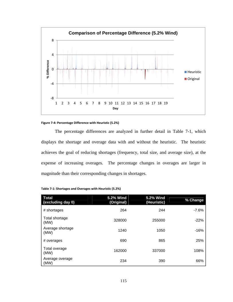
115  

Figure 7‐4: Percentage Difference with Heuristic (5.2%)

The percentage differences are analyzed in further detail in Table 7-1, which

displays the shortage and overage data with and without the heuristic. The heuristic

achieves the goal of reducing shortages (frequency, total size, and average size), at the

expense of increasing overages. The percentage changes in overages are larger in

magnitude than their corresponding changes in shortages.

Table 7‐1: Shortages and Overages with Heuristic (5.2%) 

Total (excluding day 0) 

5.2% Wind(Original)

5.2% Wind (Heuristic) 

% Change

# shortages 264 244 -7.6%

Total shortage (MW) 

328000 255000 -22%

Average shortage (MW) 

1240 1050 -16%

# overages  690 865 25%

Total overage (MW) 

162000 337000 108%

Average overage (MW) 

234 390 66%

‐8

‐4

0

4

8

% D

iffe

ren

ce

Day

Comparison of Percentage Difference (5.2% Wind)

Heuristic

Original

116  

Table 7-2 displays the rounded values of the cost distribution for the 5.2%

simulation with and without the heuristic. The total cost of slow generation increases by

only 0.3%, and the total cost of fast generation increases slightly more due to more

output. The total shortage penalty decreases significantly and outweighs the increase in

generation costs, which brings down the total cost and reduces the proportion of total cost

attributed to shortages.

Table 7‐2: Cost Distribution with Heuristic (5.2%) 

Cost ($ ) (excluding day 0)

5.2% Wind(Original)

5.2% Wind (Heuristic) 

% Change

Slow power cost 238 238 0.3%

Fast power cost  125 126 0.8%

Shortage penalty  33 25 -24%

Total cost  396 389 -1.7%

7.4 20.4% Simulation with Heuristic

When the 20.4% simulation is run with the horizon-increasing heuristic, the total

cost decreases from $3.91 10 to $3.84 10 , or a reduction of 2.26% compared to

the original 20.4% simulation. The heuristic does not change the scheduled slow power.

According to Figure 7-5, it is not the case that the 20.4% heuristic simulation fails

to increase fast power, which may have otherwise induced the day-ahead model to

schedule less slow power. The heuristic does cause the hour-ahead model to commit

more fast generation. The 20.4% heuristic simulation, in fact, commits more additional

fast generation relative to the 20.4% base case than the 5.2% heuristic does relative to the

5.2% base case, both in absolute and percentage terms: an additional 372400 MW

117  

compared to 329700 MW, or equivalently, an additional 0.69% of base case fast

generation compared to 0.36%.

Figure 7‐5: Fast Power with Heuristic (20.4%) 

The largest negative percentage change in fast generation is 97%, which occurs

during hour 54 (day 2) of the simulation. The negative percentage changes are not visible

from the graph because the positive percentage changes dwarf the negative changes. The

former reach levels as high as 13350% of base case fast generation. The negative

percentage changes, in contrast, are capped at 100% since generation cannot be

negative. Unlike the 5.2% simulation, outliers in the 20.4% simulation cannot be

removed because they account for a much larger proportion of the increases in fast

generation: 224 of the 600 positive percentage increases exceed 200% in this heuristic

simulation, compared to 1 out of 1029 in the 5.2% heuristic simulation.

The base case fast generation in the 20.4% simulation is almost zero for many

time increments because wind and slow generation are enough to satisfy demand. An

‐2000

0

2000

4000

6000

8000

10000

12000

14000

‐40000

‐30000

‐20000

‐10000

0

10000

20000

30000

40000

%

Po

wer

(M

W)

Day

Effect of Heuristic on Fast Power (20.4% Wind)

% Change

Heuristic

Original

118  

increase in fast generation from these low values causes the percentage increase to often

exceed 1000%. The outliers occur, therefore, because the hour-ahead model commits

power more liberally to anticipate shortages, which achieves the heuristic’s objective.

Figure 7-6 compares the percentage difference between total actual power and

total actual demand for the 20.4% simulation with and without the heuristic. Negative

values represent shortages. With the heuristic, overages are more common and larger in

magnitude. Shortages, on the other hand, are less severe.

Figure 7‐6: Percentage Difference with Heuristic (20.4%)

Table 7-3 shows the rounded statistics for shortages and overages in the 20.4%

simulation. Although the number of shortages increases with the heuristic, the total and

average shortage both decrease greatly. In addition, the number of overages and total

overage increase, which is expected, but the average overage decreases. The increase in

number of shortages and the decrease in average overage are the different outcomes

compared to the 5.2% heuristic simulation results.

‐15

‐10

‐5

0

5

10

15

20

25

% D

iffe

ren

ce

Day

Comparison of Percentage Difference (20.4%)

Heuristic

Original

119  

Table 7‐3: Shortages and Overages with Heuristic (20.4%) 

Total (excluding day 0) 

20.4% Wind(Original)

20.4% Wind (Heuristic) 

% Change

# shortages 158 165 4.4%

Total shortage (MW) 

247000 175000 -29%

Average shortage (MW) 

1560 1060 -32%

# overages  2591 2759 6.5%

Total overage (MW) 

8930000 9230000 3.4%

Average overage (MW) 

3450 3350 -2.9%

Table 7-4 shows the rounded cost distribution of the 20.4% simulation. The total

cost of slow power does not change, whereas the total cost of fast power increases

slightly and the total shortage penalty decreases greatly.

Table 7‐4: Cost Distribution with Heuristic (20.4%) 

Cost ($ ) (excluding day 0)

20.4% Wind(Original)

20.4% Wind (Heuristic) 

% Change

Slow power cost 195 195 0%

Fast power cost  71 72 0.8%

Shortage penalty  24.7 17.5 -29%

Total cost  291 284 -2.3%

7.5 40% Simulation with Heuristic

The 40% simulation consists of 40.0% wind penetration for the base case and

39.9% wind penetration for the heuristic case. The wind penetration decreases because

the heuristic generates enough additional fast power such that total wind power becomes

120  

a smaller percentage of total power. For convenience, these simulations are referred to as

the 40% simulation with and without the heuristic.

The total cost decreases from $4.02 10 to $3.89 10 after implementing

the heuristic, or a reduction of 3.29%. As with the 20.4% simulation, the slow generation

with the heuristic is identical to the original slow generation.

Figure 7-7 shows the change in fast generation as a result of the heuristic for the

40% simulation. A positive percent change indicates that the hour-ahead model commits

more fast generation with the heuristic. The large positive percent changes tend to occur

when the heuristic fast power does not coincide with the original fast power; in the graph,

the green bars tend to occur at the same time increments where the blue lines do not

coincide with the red lines. In other words, the heuristic causes the hour-ahead model to

commit fast generation where it previously does not commit generation, which is why the

percent changes are very large—sometimes exceeding 10000%. This phenomenon

results from the generosity with which the heuristic hour-ahead model commits fast

generation to prevent possible shortages.

The largest negative percentage change in fast generation is 90% and occurs

during hour 56 (day 2) of the simulation. As is the case with the 20.4% heuristic

simulation, the negative percentage changes are not visible in the graph because they are

dwarfed by the positive outliers. Out of 591 total time increments where committed fast

power increases when using the 40% heuristic, 331 of those occurrences represent a

percentage change exceeding 200%. Positive outliers become more common when wind

penetration increases.

121  

Figure 7‐7: Fast Power with Heuristic (40%)

Figure 7-8 compares the percentage difference for the 40% simulation with and

without the heuristic. Negative values indicate shortages. The number of shortages

increases with the heuristic, but the total shortage decreases.

Figure 7‐8: Percentage Difference with Heuristic (40%)

‐5000

0

5000

10000

15000

20000

25000

‐9000

0

9000

18000

27000

36000

45000

%

Po

wer

(M

W)

Day

Effect of Heuristic on Fast Power (40% Wind)

% Change

Heuristic

Original

‐30

‐15

0

15

30

45

60

% D

iffe

ren

ce

Day

Comparison of Percentage Difference (40% Wind)

Heuristic

Original

122  

Table 7-5 presents the rounded shortage and overage data for the 40% simulation.

As is the case with the 20.4% simulation, the number of shortages increases with the

heuristic, but total and average shortage both decrease. The number of overages and total

overage increase with the heuristic, but the average overage decreases.

Table 7‐5: Shortages and Overages with Heuristic (40%) 

Total (excluding day 0) 

40.0% Wind(Original) 

39.9% Wind (Heuristic) 

% Change

# shortages 445 461 3.6%

Total shortage (MW) 

2190000 2110000 -3.5%

Average shortage (MW) 

4920 4580 -6.8%

# overages  3376 3472 2.8%

Total overage (MW) 

51100000 51600000 0.9%

Average overage (MW) 

15100 14900 -1.9%

Table 7-6 depicts the rounded cost distribution for the 40% simulation. The cost

of slow power is again identical, whereas the cost of fast power increases by 1.3%. The

shortage penalty decreases by a larger absolute value in the 40% simulation than in the

5.2% and 20.4% simulations, but the percentage decrease is smaller.

Table 7‐6: Cost Distribution with Heuristic (40%) 

Cost ($ ) (excluding day 0)

40.0% Wind(Original)

39.9% Wind (Heuristic) 

% Change

Slow power cost 116 116 0%

Fast power cost  68 69 1.3%

Shortage penalty  219 205 -6.5%

Total cost  402 389 -3.3%

123  

7.6 Comparison of Heuristic Simulations

This section compares the percentage changes of various metrics as a result of the

heuristic for all three simulations. Table 7-7 shows the comparison of shortage and

overage data with respect to the base cases. The percentage decrease in total shortage

increases with higher wind penetration for the first two simulations but then decreases

dramatically for the 40% simulation. The reason is that the size of the original total

shortage for the 40% simulation is so large (2190000 MW compared to 328000 MW for

the 5.2% simulation) that even though the heuristic decreases the total shortage by

roughly the same amount (76200 MW compared to 72900 MW for the 5.2% simulation),

the percentage decrease is much smaller.

The table also shows that the percentage change in the number of overages, total

overage, and average overage actually decrease with increasing wind penetration, which

may not be obvious. Although the absolute values become larger with wind penetration,

this result implies that the hour-ahead model does not go overboard with its tendency to

err on the side of overages, thereby limiting the increase in excess generation.

Table 7‐7: Shortages and Overages (5.2%, 20.4%, 40%) 

% Change compared to Base Case (excluding day 0) 

5.2% heuristic 20.4% heuristic  40% heuristic

# shortages -7.6% 4.4% 3.6%

Total shortage (MW) 

-22% -29% -3.5%

Average shortage (MW) 

-16% -32% -6.8%

# overages  25% 6.5% 2.8%

Total overage (MW) 

108% 3.4% 0.9%

Average overage (MW) 

66% -2.9% -1.9%

124  

Table 7-8 compares the percentage change in cost distribution with respect to the

base cases. The cost of slow power does not change for the 20.4% and 40% heuristic

simulations. The percentage change in the cost of fast power, unexpectedly, does not

increase greatly with wind penetration. This observation may be an indicator that the

heuristic does not generate additional power excessively. The percentage change in the

shortage penalty decreases dramatically in the 40% simulation, again due to its initial

large value in the 40% base case. Finally, the percentage decrease in the total cost of

simulation increases with wind penetration, which implies an increasing marginal benefit

of the heuristic and suggests that increasing the horizon of the hour-ahead model may

reduce costs even with large wind penetration.

Table 7‐8: Cost Distribution with Heuristic (5.2%, 20.4%, 40%) 

% Change compared to Base Case (excluding day 0) 

5.2% heuristic 20.4% heuristic  40% heuristic

Slow power cost 0.3% 0% 0%

Fast power cost  0.8% 0.8% 1.3%

Shortage penalty  -24% -29% -6.5%

Total cost  -1.7% -2.3% -3.3%

Table 7-9 shows the changes in fast generation due to the heuristic. The

percentage increase in fast generation becomes larger with wind penetration because base

case fast generation is the lowest for high wind penetration. The number of time periods

where fast generation increases, however, actually decreases with wind penetration,

which means that the additional generation is concentrated into fewer time periods. This

result is also reflected in the distribution of outliers. Percentage increases in fast

generation greater than 200% are classified as outliers, and percentage increases greater

125  

than 10000% are classified as super-outliers. As wind penetration increases, outliers and

super-outliers account for a larger percentage of the increases in fast generation.

Table 7‐9: Changes in Fast Generation with Heuristic (5.2%, 20.4%, 40%) 

Fast Generation compared to Base Case (excluding day 0) 

5.2% heuristic 20.4% heuristic  40% heuristic

% increase in total fast generation (10 MW)

0.36% 0.69% 1.3%

# time increments with increased fast generation 

1029 600 591

# (%) time increments with % change > 200% 

0 (0%) 224 (37.3%) 331 (56.0%)

# (%) time increments with % change > 10000% 

0 (0%) 7 (1.2%) 20 (3.4%)

The number of time increments with increased fast generation is a relatively small

percentage of the total number of time increments. For the 40% simulation, they account

for 10.3% of all time increments. Thus, the hour-ahead model does not increase

fast generation at a majority of time periods, which is the heuristic’s intention (otherwise,

too much power would be wasted). The heuristic is designed such that the increases in

fast generation would ideally occur in the last time increment of the hour, ceteris paribus,

to alleviate potential shortages yet minimize excess generation. In practice, 10.8%

of all increases occurred during the last time increment 11 of any hour (as well as

10.3% of all outlier increases). These values are only slightly larger than what

they would be if they followed a uniform distribution of 8.3% across all time

periods, suggesting that the heuristic should be further fine-tuned so that more increases

occur at the end of each hour.

126  

7.7 Generalization using a Tunable Parameter

If the difference between current slow generation and slow generation for the next

hour is positive, the heuristic adds this difference to the demand that must be satisfied by

the hour-ahead model. Suppose, instead, that a multiple of the difference is a more

optimal quantity to add in order to balance the costs of overage and shortage. Let 0

be a tunable parameter. Then the heuristic can be generalized as follows:

,, , , , 0

0∀ ∈ 0, 1 , 1

Different values of lead to different simulation outcomes, so an optimal may

be found. The previous formulation of the heuristic is , , 1 for all three wind

penetration simulations. Now the tunable parameter is varied: 1, 2, and 3

are each tested for the 40% simulation. It is not claimed that any of the tested tunable

parameters is optimal; rather, the intention is to show how varying the tunable parameter

reveals tradeoffs in the underlying problem.

The wind penetration for each of the three tunable parameter simulations is

39.9%, but they are collectively referred to as the 40% simulation for convenience. The

total costs are $3.892 10 , $3.854 10 , and $3.845 10 , respectively. Thus,

the cost decreases with , which makes sense since the hour-ahead model commits more

fast generation as increases to prevent possible shortages. The result is not as intuitive

as it appears, however, because as increases, the decrease in shortage penalty is

accompanied by higher generation costs. Then the tradeoff between more overage and

less shortage becomes less obvious.

127  

Figure 7‐9: Percentage Difference with Tunable Parameter (40%)

Figure 7-9 compares the percentage difference in total actual power and total

actual demand for each value of the tunable parameter. More overages occur as

increases. Many of the additional overages also occur at the same time increments. For

example, many overages for 3 are extensions of overages for 2.

Table 7-10 compares the percentage changes in shortage and overage data for the

40% simulation using the 1, 2, and 3 heuristics. Percentage changes are

based on the original 40.0% simulation. No clear pattern exists for shortages: 2

reduces both the number of shortages and the total shortage by the greatest percentage,

but it has the smallest effect on reducing the average shortage. The effects on overage

are more straightforward. As increases, the number of overages, total overage, and

average overage all increase, which makes sense because the demand that must be

satisfied, and therefore additional generation, increases with .

‐30

‐15

0

15

30

45

60

75

90

% D

iffe

ren

ce

Day

Percentage Difference by Tunable Parameter (40% Wind)

rho = 3

rho = 2

rho = 1

128  

Table 7‐10: Shortages and Overages with Tunable Parameter (40%) 

40% Simulation (excluding day 0) 

% Change( )

% Change( )

% Change ( ) 

Original

# shortages 0.45% -1.1% 3.6% 445

Total shortage (MW) 

-3.7% -3.8% -3.5% 2190000

Average shortage (MW) 

-4.1% -2.7% -6.8% 4920

# overages  3.4% 3.0% 2.8% 3376

Total overage (MW) 

1.9% 1.5% 0.9% 51100000

Average overage (MW) 

-1.4% -1.4% -1.9% 15100

Table 7-11 compares the percentage changes in cost distribution for each value of

. The cost of fast power increases (at a slightly decreasing rate) as increases. The

shortage penalty decreases as increases, but the magnitude of percentage change

experiences diminishing marginal improvement. There is an additional 1.9% decrease in

shortage penalty between 1 and 2 but only an additional 0.5% decrease between

2 and 3. Despite these decreasing marginal gains, the total simulation cost is

the lowest with 3. The tradeoff between the costs of overage and shortage, however,

suggests that increasing will eventually increase the total cost.

Table 7‐11: Cost Distribution with Tunable Parameter (40%) 

40% Simulation (excluding day 0) 

% Change( )

% Change( )

% Change ( ) 

Original Cost($ )

Slow power cost 0% 0% 0% 116

Fast power cost  2.4% 2.0% 1.3% 68

Shortage penalty  -8.9% -8.4% -6.5% 219

Total cost  -4.5% -4.2% -3.3% 402

129  

Table 7-12 compares the fast generation data for each value of . As increases,

the number of time periods with more fast generation than the base case also increases,

suggesting a limitation of the heuristic since the additional fast generation should ideally

be concentrated in fewer time periods to avoid excess generation. The percentage

occurrence of outliers (time increments with 200% additional fast generation with the

heuristic) stays relatively constant, but the percentage occurrence of super-outliers (time

increments with 10000% additional fast generation with the heuristic) more than doubles

when increases to 2 or 3, which is a sign of excess generation.

Table 7‐12: Changes in Fast Generation with Tunable Parameter (40%) 

40% Simulation (excluding day 0) 

heuristic  heuristic   heuristic

% increase in fast generation over base case (10 MW)

2.5% 2.0% 1.3%

# time increments with increased fast generation 

661 613 591

# (%) time increments with % change > 200% 

374 (56.6%) 335 (57.9%) 331 (56.0%)

# (%) time increments with % change > 1000% 

49 (7.4%) 45 (7.3%) 20 (3.4%)

The above sensitivity analysis for 1, 2, and 3 holds true only for the

40% simulation. A sensitivity analysis on may be very different for the 5.2% and

20.4% simulations, which are not presented. The effect of changing the tunable

parameter, in addition, depends on other characteristics of the simulation, such as the use

of linear interpolation to obtain sub-hourly actual wind and demand values. As a result,

the benefit of using a heuristic to increase the effective horizon of the hour-ahead model

depends heavily on the assumptions of the simulation. A better idea, therefore, may be to

change directly the implementation of the hour-ahead model so that the horizon is

actually increased. A proposal to achieve this outcome is presented below.

130  

7.8 Proposal to Increase the Horizon of the Hour-Ahead

Model

The main takeaway from the heuristics analysis is that increasing the horizon of

the hour-ahead model reduces the total cost. Different implementations of this heuristic

would achieve a similar purpose, and the incorporation of tunable parameters allows for

the optimization of the heuristic over many simulations. Finding a more suitable

functional form of the heuristic, furthermore, may lead to even more cost reductions. For

example, extra generation could be added to the demand of additional sub-hourly

increments, not just the last component. Alternatively, a proportion 0 1 of extra

generation could be added if future slow generation were greater than current slow

generation, in case actual wind were low enough to still cause a shortage. Ultimately,

however, the heuristic is merely an approximation to increase the effective horizon of the

problem without changing the implementation of the hour-ahead model.

A more direct way to reduce costs, therefore, is to change the implementation of

the hour-ahead model to increase its horizon. This change requires the replacement of

the existing hour-ahead transition function by another function . This

section proposes a lookahead policy to extend the horizon of the hour-ahead model by

five minutes.

Let 13 be the number of time increments in the new horizon. 12 is still

the number of time increments per hour insofar as only 12 of the 13 solutions per

decision vector are implemented: the 13th solution is used as a placeholder to gain insight

131  

into the next hour – thereby increasing the horizon – but is not implemented. The

simulation model did not previously distinguish between the number of time increments

in the horizon and the number of solutions that are implemented. This proposed

extension of the hour-ahead model’s horizon introduces this distinction. As a result, the

simulation model established in Chapter 4 undergoes the following changes.

7.8.1 State Variable

The adjusted state variable at day , hour is the following:

, , ,

where is the state variable for the day-ahead model for day and , is the

adjusted state variable for the hour-ahead model for day , hour .

Note that the day-ahead model and the day-ahead state variables do not change:

the horizon is increased in the hour-ahead model only. It is still true, therefore, that:

Χ ,

, , ,

The notation for the hour-ahead state variable changes to reflect the new

distinction between the length of the horizon and the length of the implemented solution.

The actual computation of the state variable, however, remains the same:

, , , |

The inter-hour transition variables as defined in the hour-ahead model from

Chapter 3 are still calculated at time , not at time . As a result, the decisions that are

scheduled to occur during time increment 1 in the simulation are not taken into

account when transitioning to the next hour , 1 . The decision variables

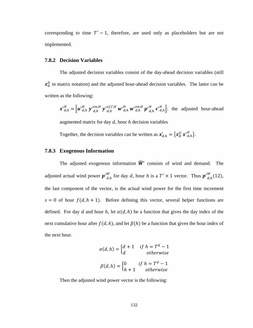
132  

corresponding to time 1, therefore, are used only as placeholders but are not

implemented.

7.8.2 Decision Variables

The adjusted decision variables consist of the day-ahead decision variables (still

in matrix notation) and the adjusted hour-ahead decision variables. The latter can be

written as the following:

, , ,, ,

, , ,, , , : the adjusted hour-ahead

augmented matrix for day , hour decision variables

Together, the decision variables can be written as , , .

7.8.3 Exogenous Information

The adjusted exogenous information consists of wind and demand. The

adjusted actual wind power , for day , hour is a 1 vector. Thus , 12 ,

the last component of the vector, is the actual wind power for the first time increment

0 of hour , 1 . Before defining this vector, several helper functions are

defined. For day and hour , let , be a function that gives the day index of the

next cumulative hour after , , and let be a function that gives the hour index of

the next hour.

, 1 1

, 0 11

Then the adjusted wind power vector is the following:

133  

,, 1

Ω , , , 0 ∀ ∈ 0, 1

Likewise, let , be the adjusted total load vector with length . Thus

, 12 is the total load for time 0 of hour , 1 . Then , satisfies:

,, 1

Λ , , , 0 ∀ ∈ 0, 1

This method does not look into the future because the first demand value of the

next hour is already used in the method of linear interpolation. If predicted values were

used instead of actual values, then this method would be inadequate because it would be

non-adaptive. Predicted wind and demand, however, are outside the scope of this thesis.

N.B.: An arbitrary number may replace the values Ω , , , 0

and Λ , , , 0 for the last hour of the last day of simulation when there is

no natural lookahead value.

7.8.4 Transition Functions

The adjusted transition function computes the adjusted state variable at the

next hour from the adjusted inputs at the current hour of day .

, , , , Χ, Χ ,

, , , ,

The first step in computing , , is to compute Χ ,, . Recall that ,

is the total scheduled slow generation at hour of day . Then , , is the total

scheduled slow generation at the next hour. Define , as the adjusted total load vector

of length 1 that must be satisfied by the fast generators only. Then it is calculated as

follows:

134  

,, 1

, , , , ∀ ∈ 0, 1

The hour-ahead mixed integer linear programming algorithm is not adjusted

because the length of the output decision vectors is automatically the length of the input

vector. Since the input , has length instead of , the output augmented decision

variable matrix , has length instead of . Then the output of the hour-ahead

model Χ , is:

Χ ,, , , ,

, ,, ,

, , ,, , ,

The implementation of the solution must be adjusted because now not all of the

components of the decision vectors are implemented. In particular, the last component

corresponding to 1 is not implemented. Recall that Μ is a mapping of indices

such that index in maps to index Μ in . After each hour of the simulation,

certain day-ahead solutions are updated by their hour-ahead counterparts via the

following adjusted transition functions:

, , 1, , ∀ ∈

, , 1, , ∀ ∈

, , 1, , ∀ ∈

Note that the values on the right hand side are the second-to-last entries of each

decision column vector, instead of the last entry. Only time increment 11 solutions

are updated to the day-ahead solution because only solutions corresponding to ∈ 0,11

135  

are implemented. The last solution corresponding to 12 is scheduled by the hour-

ahead model but not implemented.

The transition functions for the instantaneous decision variables, on the other

hand, are not different. The reason is that the set of instantaneous hit times already looks

only within the interval ∈ 0,11 . Recall that:

, , ∈ : ∈ 0, 1 , , , 1 , ∀ ∈ , , , ∈

Whatever instantaneous decision that is scheduled to occur during time increment

12, therefore, is ignored.

7.8.5 Objective Function

The objective function undergoes a slight change of notation for the updated

decision matrices. The underlying idea, however, is the same since the summation occurs

over ∈ 0,11 and, therefore, does not take into account the time increment that is not

implemented. It can be written as:

min , ,, , ,

∈ ,∈ ,∈

, , ,,

,, , , ,

∈ ,∈ ,∈ ,∈

,, ,

These proposed changes to the simulation model reflect a possible

implementation of increasing the horizon of the hour-ahead model by a single five minute

increment. They are presented here as a possible reference for further research. The

extension to multiple additional increment horizons is not presented here but can be done

136  

by increasing the vector length of the decision variables solved by the mixed integer

linear program but implementing only the initial solutions. Extending the horizon

beyond 24 five minute increments may prove difficult but also unnecessary, since the

increased horizon becomes less useful as it approaches double the size of the original

horizon.

137  

Chapter VIII

8 Conclusions and Extensions

This chapter reviews the conclusions of the simulations from Chapters 6 and 7

and discusses the implications of increasing RTOs’ wind penetration. The chapter closes

by presenting limitations of the hour-ahead and simulation models and suggesting

improvements for future areas of research.

8.1 Results and Implications

Simulations were run at 5.2%, 20.4%, and 40.0% wind penetration. The

percentage difference between total actual power and demand is always correlated with

wind power because less generated power is required as wind increases.

8.1.1 Increasing Wind Penetration

The simulation cost decreases by about 26.4% as wind penetration increases from

5.2% to 20.4%. Wind power is assumed free, and since wind accounts for a higher

percentage of the total power, the total cost decreases. Several reasons explain why the

cost decrease is not higher, given that the amount of wind is almost four times as large in

the 20.4% simulation. First, the hour-ahead model does not adjust the output of the slow

generators, so overages are more common with 20.4% wind. The excess slow generation

is wasted whenever wind and slow generation combine to exceed demand. Second, wind

power is not stable but rather extremely noisy, as shown in Chapter 5. Since large

138  

amounts of wind tend to arrive in concentrated time increments, especially when demand

has already been satisfied, the cost reduction is not as large as the fourfold increase in

wind penetration would suggest.

As wind penetration increases from 20.4% to 40.0%, total cost increases by 38%.

Although the additional wind power is free, the volatile nature of wind more than doubles

the number of shortages. Compared to the 5.2% simulation, however, total cost increases

only by 9.9%. When wind penetration increases from 5.2% to 40.0%, the proportion of

cost attributable to generation decreases from 92% to 46%. Furthermore, the number of

shortages increases 69%, and the total shortage increases over 500%. The large variation

in wind power decreases the hour-ahead model’s accuracy in committing fast generation.

Overages, on the other hand, increase in frequency and magnitude. Allowing the hour-

ahead model to modify slow generation would reduce the overage and, therefore,

unnecessary generation costs. Although increasing wind penetration to 40.0% provides

more free power, the volatility of wind and the resulting shortage penalties outweigh the

savings in generation costs. The benefits of increasing wind penetration to 20.4%, on the

other hand, outweigh the shortage penalties. Thus, increasing the amount of renewable

energy too soon too fast may in fact prove detrimental in preserving the efficiency of the

power system. Gradually increasing the wind penetration from current levels to around

20% seems to be the better option.

8.1.2 Increasing the Horizon

Shortages tend to occur at the first time increment of each hour. Excluding day 0

in the 5.2% simulation, for example, 67% of the 264 shortages occur during 0. This

tendency is a limitation of the hour-ahead model. A heuristic to increase the effective

139  

horizon of the hour-ahead model is tested for each wind penetration simulation, and it

indeed decreases total cost of the 5.3%, 20.4%, and 40% simulations by 1.7%, 2.3%, and

3.3%, respectively. There are two implications: first, increasing the horizon of the model

results in better scheduling of generators, and second, the marginal benefit of increasing

the model’s horizon decreases with higher wind penetration. Furthermore, improving the

heuristic by using a tunable parameter improves cost reduction for the 40% simulation by

an additional 1.2%.

8.2 Limitations

The hour-ahead model makes assumptions to simplify the problem and be

compatible with the available data. These assumptions limit how closely the model

represents the hour-ahead unit commitment problem faced by RTOs. Recognizing these

limitations, therefore, is important to understanding how realistic and applicable the

results are.

The major limitation of the hour-ahead model is that it uses actual wind and

demand values instead of predictions. This aspect lets the hour-ahead model peek into

the future at the beginning of each hour and see exactly what will happen until the end of

the hour. This assumption is certainly unrealistic. The simulation results, therefore, are

in a sense a best-case scenario for how well an RTO can respond to the volatility of wind

and demand. Once predicted values are used and the hour-ahead model’s solutions are

compared against actual values, shortages will most likely become more common

because more uncertainty will be introduced to the problem.

140  

Another limitation is the hour-ahead model’s limited horizon, which is explored

in Section 6.1. The model schedules a solution to satisfy actual demand for the current

hour. What happens during the next hour does not factor into the solution. In real-life,

however, the horizon of an RTO’s problem will include at least some information past

the horizon of its generation schedule because that information is crucial for inter-day

and inter-hour transitions.

Third, the simulation assumes wind power is free. In reality, wind power incurs a

marginal cost just like any other source of power, so the integration of wind into the

system is not as straightforward as the simulations suggest. The day-ahead model may

not automatically schedule as much wind as the forecasts suggest, and the hour-ahead

model may not use all of the available wind.

Fourth, this simulation lacks a grid network. The model assumes that power from

any generator in the system can be used to satisfy demand coming from anywhere in the

system. It ignores the cost to transport power from source to destination. Including a

grid network in the model is more realistic because it takes into account the locations of

generation and usage during the optimization.

8.3 Extensions and Further Areas of Research

Extensions should relax the assumptions that are necessary for the hour-ahead

model and the simulation model. First, the hour-ahead model should take in predicted

wind and demand, which would require an algorithm for generating predictions. This

extension would prevent the hour-ahead model from looking into the future at every hour.

141  

Second, the hour-ahead model’s horizon should be extended by five minutes, and

the simulation model should implement all but the last solution. Section 7.8 provides a

blueprint for the increase in horizon, which can be generalized to ten or fifteen minutes.

As seen in the heuristic studies from Chapter 7, this extension should reduce total costs.

Third, the hour-ahead model should represent PJM’s problem more realistically.

A straightforward improvement would be to use more accurate data, such as ramp rates

that are functions of output and actual generator costs instead of bid costs. Another

improvement would be to allow the hour-ahead model to change the slow generation of

online generators, which would decrease both overage and cost. A more complex

improvement would be to implement a cool-down state and a minimum cool-down time

so that generators do not transition directly between the online and off states.

Fourth, the hour-ahead model’s slack generation decision variables are the dual

variables to the day-ahead model’s problem. Similarly, the day-ahead model’s slack

generation decision variables provide information to the hour-ahead model. Exchanging

this information between the two models would allow each to learn from its past

performance and adjust its generation schedule for future performance. Such an

algorithm may prove helpful in reducing total cost.

Finally, the smaller time horizon of the hour-ahead model is an appropriate setting

to use battery storage. Energy dissipation is usually the limitation of batteries, but if they

are used to store power from one five minute increment to the next, leakage becomes less

of an issue. The prevention of unexpected shortages on the intra-hourly time scale

involves a tradeoff between using storage and using expensive fast generation, so using

battery storage could reduce total cost.

142  

8.4 Final Remarks

Power generation is vital for the functioning of the U.S. economy. In today’s

world, even a brownout could negatively impact the daily affairs of both businesses and

individuals. Thus, PJM and other RTOs face the increasingly important problem of

scheduling generation to meet forecasted demand. When considering the contemporary

issue of renewable energy and the ongoing effort to integrate more wind into the system,

this problem becomes even more complex. The ability of RTOs to create a day-ahead

schedule that satisfies demand while minimizing total system cost depends heavily on the

accuracy of wind and demand forecasts. Applying mixed integer linear programming to

solve the hour-ahead unit commitment problem, therefore, is an effective way of

adjusting the day-ahead schedule and improving the performance of RTOs. Additional

research to incorporate short-term battery storage can take this progress further in order

to improve both the dependability and the environmental friendliness of the U.S. power

network.

143  

References

Austen, I. (2012). Pengrowth Energy to Buy NAL Energy. DealBook. The New York Times. Retrieved from http://dealbook.nytimes.com/2012/03/23/pengrowth- energy-to-buy-nal-energy/.

Barth, R., Brand, H., Meibom, P., & Weber, C. (2006). A Stochastic Unit-commitment Model for the Evaluation of the Impacts of Integration of Large Amounts of Intermittent Wind Power. 9th International Conference on Probabilistic Methods Applied to Power Systems. KTH Royal Institute of Technology. Retrieved from http://ieeexplore.ieee.org/stamp/stamp.jsp?tp=&arnumber=4202207&tag=1.

Berst, J. (2011). Is Natural Gas an Enemy to the Smart Grid? Smart Grid News. Retrieved from http://www.smartgridnews.com/artman/publish/

Business_Strategy/Is-natural-gas-an-enemy-to-the-smart-grid-3796.html.

Botterud, A., Wang, J., Miranda, V., Bessa, R., Keko, H., & Akilimali, J. (2010). Wind Power Forecasting and Electricity Market Operations. IAWind 2010. Retrieved from http://www.iawind.org/presentations/botterud.pdf.

Botterud, A., Wang, J., Monteiro, C., & Miranda, V. (2009). Wind Power Forecasting and Electricity Market Operations. San Francisco IAEE Conference 2009. Retrieved from http://www.usaee.org/usaee2009/submissions/OnlineProceedings/

Botterud_etal_paper.pdf.

Boyce, M. P. (2010). Handbook for Cogeneration and Combined Cycle Power Plants. New York, NY: ASME Press.

Bryce, R. (2011). Texas Wind Energy Fails, Again. National Review. Retrieved from http://www.nationalreview.com/articles/275673/texas-wind-energy-fails-again-

robert-bryce.

Bureau of Labor Statistics. (2010). Consumer Price Index Detailed Report. United States Department of Labor. Retrieved from http://www.bls.gov/cpi/cpid1010.pdf.

California ISO. (2012). Today’s Outlook. Retrieved from http://www.caiso.com/Pages/

Today's-Outlook-Details.aspx.

144  

Chang, G. W., Tsai, Y. D., Lai, C. Y., & Chung, J. S. (2004). A Practical Mixed Integer Linear Programming Based Approach for Unit Commitment. IEEE Power Engineering Society General Meeting. Retrieved from http://ieeexplore.ieee.org/stamp/stamp.jsp?arnumber=01372789.

Combs, S. (2012). Window on State Government. Texas Comptroller of Public Accounts.

Retrieved from http://www.window.state.tx.us/specialrpt/energy/nonrenewable/ coal.php.

Cordaro, M. (2008). Understanding Base Load Power: What it is and Why it Matters. New York Affordable Reliable Electricity Alliance. Retrieved from http://www.area-alliance.org/documents/base%20load%20power.pdf.

de la Merced, M. J. (2012a). El Paso Corp. Sells Units to Apollo-Led Group for $7.15 Billion. DealBook. The New York Times. Retrieved from

http://dealbook.nytimes.com/2012/02/24/el-paso-sells-divisions-to-apollo- led-group-for-7-15-billion/.

de la Merced, M. J. (2012b). Mitsubishi Buys 40% Stake In Encana Shale Gas Assets. DealBook. The New York Times. Retrieved from http://dealbook.nytimes.com/

2012/02/17/encana-strikes-2-9-billion-shale-deal-with-mitsubishi/.

Ebrahimi, J., Hosseinian, S. H., & Gharehpetian, G. B. (2011). Unit Commitment Problem Solution Using Shuffled Frog Leaping Algorithm. IEEE Transactions on Power Systems, 26(2). Retrieved from http://ieeexplore.ieee.org/stamp/

stamp.jsp?tp=&arnumber=5530389.

Fossil Energy Office of Communications. (2011). U.S. Department of Energy. Retrieved from http://fossil.energy.gov/programs/powersystems/turbines/

turbines_howitworks.html.

GenOn. (2010). GenOn Energy. Retrieved from http://www.genon.com/.

Henkel, N., Schmid, E., & Gobrecht, E. (2008). Operational Flexibility Enhancements of Combined Cycle Power Plants. POWER-GEN Asia 2008. Retrieved from http://www.energy.siemens.com/hq/pool/hq/energy-topics/pdfs/en/combined- cycle-power-plants/OperationalFlexibilityEnhancementsofCombinedCyclePower

Plants.pdf.

145  

Kehlhofer, R., Rukes, B., Hannemann, F., & Stirnimann, F. (2009). Combined-Cycle Gas and Steam Turbine Power Plants. Retrieved from http://www.knovel.com/

web/portal/basic_search/display?_EXT_KNOVEL_ DISPLAY_bookid=3612.  

Kendig, M. (2011, November 2). Telephone interview.

MacIntosh, N. (2011, October 31). Telephone interview.

Padhy, N. P. (2004). Unit Commitment—A Bibliographical Survey. IEEE Transactions on Power Systems, 19(2). Retrieved from http://www.ieexplore.ieee.org/ stamp/stamp.jsp?arnumber=01295033.

PJM. (2012). “About PJM.” Retrieved from http://pjm.com/about-pjm.aspx.

Powell, W. B. (2010). Approximate Dynamic Programming: Solving the Curses of Dimensionality. 2nd ed. Hoboken, NJ: John Wiley & Sons, Inc.

Rebenitsch, R. (2011). Wind & the LMS 100. UWIG Annual Meeting.

Roose, K. (2012). Blackstone Makes $2 Billion Natural Gas Investment. DealBook. The New York Times. Retrieved from http://dealbook.nytimes.com/2012/02/27/

blackstone-makes-2-billion-natural-gas-investment/.

Shepard, R. (2010). Gas Turbine Technologies for Electric Generation. Neel-Schaffer Engineering Professional Development Seminar.

Takriti, S., Birge, J. R., & Long, E. (1996). A Stochastic Model for the Unit Commitment Problem. IEEE Transactions on Power Systems, 11(3). Retrieved from http://ieeexplore.ieee.org/stamp/stamp.jsp?tp=&arnumber=535691.

Tennessee Valley Authority. (2011). Combustion Turbine Power Plant. Retrieved from http://www.tva.gov/power/cumb_turbineart.htm.

Tucker, S., Ngai, E., & Chung, J. (2009). Electric Utilities and Power Primer. Oppenheimer.

U.S. Department of Energy. (2008). 20% Wind Energy by 2030: Increasing Wind Energy’s Contribution to the U.S. Electricity Supply. National Renewable Energy Laboratory. Retrieved from http://www.nrel.gov/docs/fy08osti/41869.pdf.

146  

U.S. EIA. (2012). Annual Energy Outlook 2012 Early Release. Retrieved from http://www.eia.gov/oiaf/aeo/tablebrowser/.

Victory Energy. (2011). Combined Cycle Utility HRSG. Retrieved from http://www.victoryenergy.com/heat-recovery-steam-generator/.

Wald, M. L. (2010). Offshore Wind Power Line Wins Backing. New York Times. Retrieved from http://www.nytimes.com/2010/10/12/science/earth/

12wind.html?hp.

Yan, J. H., & Stern, G. A. (2002). Simultaneous Optimal Auction and Unit Commitment for Deregulated Electricity Markets. The Electricity Journal, 15(9). Retrieved from http://www.sciencedirect.com/science/article/B6VSS-473J0GG-

2/s2/68312a964eb3d76eb7eec0ba54b81bb4.

Zhou, J. (2010). 20% Wind Generation and the Energy Markets. Senior Thesis, Princeton University. Retrieved from http://www.castlelab.princeton.edu/theses/

Zhou,%20Jessica-senior%20thesis%20final%20April%202010.pdf.

20% Wind Energy by 2030. (2008). 20% Wind Energy by 2030 Summary Presentation. Retrieved from http://www.20percentwind.org/20percent_Summary_

Presentation.pdf.