NATURAL GAS LIQUIDS PLANT OPTIMIZATION An Application of Linear Programming Sandro Papile RESEARCH PROJECT SUBMITTED IN PARTIAL FULFILLMENT OF THE REQUIREMENTS FOR THE DEGREE OF MASTER OF BUSINESS ADMINISTRATION in the Faculty of Business Administration @ Sandro Papile 1989 SIMON FRASER UNIVERSITY JULY 1989 All rights reserved. This work may not be reproduced in whole or in part, by photocopy or other means, without permission of the author.

Welcome message from author
This document is posted to help you gain knowledge. Please leave a comment to let me know what you think about it! Share it to your friends and learn new things together.
Transcript

NATURAL GAS LIQUIDS PLANT OPTIMIZATION
An Application of Linear Programming
Sandro Papile
RESEARCH PROJECT SUBMITTED IN PARTIAL FULFILLMENT OF
THE REQUIREMENTS FOR THE DEGREE OF
MASTER OF BUSINESS ADMINISTRATION
in the Faculty
of
Business Administration
@ Sandro Papile 1989
SIMON FRASER UNIVERSITY
JULY 1989
All rights reserved. This work may not be
reproduced in whole or in part, by photocopy
or other means, without permission of the author.

APPROVAL
I
Name : Sandro Papile
Degree : Master of Business Administration
Title of Project:
NATURAL GAS LIQUIDS PLANT OPTIMIZATION
An Application of Linear Programming
Examining Committee:
Dr. Eng Choo
Senior Supervisor
- Dr Art Warburton
Associate Professor
Date Approved: -%F\
(ii)

PARTIAL COPYRIGHT LICENSE
I hereby g ran t t o S l m n Fraser Unlvers l ty the r l g h t t o lend
my thesis, proJect o r extended essay ( the t i t l e o f which i s shown below)
t o users o f the Simon Fraser Un ive rs i t y Library, and t o make p a r t i a l o r
s ing le copies only f o r such users o r I n response t o a request from t h e
l i b r a r y o f any o ther university, o r o ther educational I ns t i t u t l on , 0"
i t s own bohalf o r f o r one of i t s users. I fu r ther agree t h a t permission
f o r mu1 t i p l o copying o f t h i s work f o r scho lar ly purposes may be granted
by mo o r tho Ooan o f Graduate Studjos. It i s understood t ha t copying
o r pub l l co t l on o f t h i s work f o r f l nanc la l galn sha l l not be alfowod
without my w r i t t on pormlsslon.
T i t I e of Thos i s/Projoct/Extended Essay
Natural Gas Liquids P l a n t Opt imiza t ion .
An A p p l i c a t i o n o f Linear Programming.
Author: Sandro Pa pi1 e
(s ignature)
ABSTRACT
,
A Linear Programming (LP) model was used to optimize
weekly production scheduling at Westcoast's Taylor Natural
Gas Liquids (NGL) Recovery Plant. The profit function was
derived and it was shown that, because of its particular
structure, profit is maximized when fluctuations between
daily productions are minimized. An LP model was developed
to calculate the smoothest production schedule; its
solution was obtained with both simple heuristic and
computer analysis. Twelve weeks of actual operating data
were used to validate the model. An indication was given
on how post-optimality analysis of the LP results could
further help in optimizing plant operation.
(iii)

APPROVAL
ABSTRACT
LIST OF TABLES
LIST OF FIGURES
TABLE OF CONTENTS
I Page
ii
iii
vii
viii
1. INTRODUCTION
1.1 General Objectives of the Study
1.2 Expected Benefits
2. THE NGL PLANT
2.1 Plant Description 6
2.2 Current Production Scheduling System 12
3. COSTS AND REVENUES
3.1 Introduction
3.2 Process Variables
3.3 Costs
3.4 Revenues
4. MODELLING
4.1 Problem Statement
4.2 The Model

Page
5. THE PROFIT FUNCTION I
5.1 The Function and Its Analysis
5.2 Comparison with Actual Runs
6. THE LP MODEL
6.1 LP Formulation
6.2 Opening and Closing Inventory
6.3 Heuristic Solution
7. THE LP SOLUTION
8. COMPARISON WITH ACTUAL OPERATION
8.1 Model Planning vs. Actual
8.2 Sensitivity Analysis
8.3 Special Cases
9. CONCLUSIONS 63
APPENDICES
A.l Production Data 66
A.2 Recompression Power Regression Analysis 72
A.3 LP Models "NEXT1" and "THIS1" 75
A.4 Summary of Results from Model "NEXT"
for Twelve Weeks 81
Page
A.5 Summary of Results $from Model "THIS" 85
A.6 Comparison Between Actuals and Model
Results 89
A.7 Post-optimality Analysis for
for Case "THISIl" 9 3

LIST OF TABLES
, Page
Table 2.1 - TYPICAL PLANT FEED AND PRODUCT COMPOSITIONS 11
3.1 - TYPICAL OPERATING COST BREAK-DOWN 21
6.1 - HEURISTIC SOLUTION OF LP - Example 45
6.2 - HEURISTIC SOLUTION OF LP - Example 2 48
7.1 - EQUATIONS FOR MODEL "NEXT" 54
7.2 - EQUATIONS FOR MODEL "THIS" 54
(vii)

LIST OF FIGURES
I
Fig. 2.1 - TAYLOR NGL PLANT - Conceptual Schematic 5.1 - FEASIBLE PROPANE PRODUCTION REGION 5.2 - PROFIT FUNCTION 5.3 - PROPANE PRODUCTION FOR MAXIMUM
PROFIT - Rich Feed 5.4 - PROPANE PRODUCTION FOR MAXIMUM
PROFIT - Design Feed 5.4 - PROPANE PRODUCTION FOR MAXIMUM
PROFIT - Lean Feed 6.1 - SCHEMATIC REPRESENTATION OF THE LP MODEL 8.1 - COMPARISON BETWEEN ACTUALS & MODEL NEXT
8.2 - COMPARISON BETWEEN ACTUALS & MODEL THIS
8.3 - CAPABILITY OF EACH PRODUCTION LINE A.l - REGRESSION ANALYSIS - Power vs. Feed
Page
7
28
31
(viii )

Page 1
1. INTRODUCTION
1.1 General Objectives of the Studv
Westcoast Energy Inc. operates a natural gas liquid
(NGL) recovery plant at Taylor, British Columbia. The
plant processes most of the natural gas produced in the
area, extracting propane, butane and condensates.
The facility generated $19.5 million in revenue during
1987 but, as pointed out in the 1987 Annual Report of the
Company, "the earnings for this project have been
disappointing to date because of the low prices prevailing
in the propane marketw.
In fact propane is increasingly difficult to sell, and
plant operation is presently adjusted to limit the amount
of propane produced to the amount expected to be sold.
Because of thermodynamic process constrains, this
translates into a limitation on the production of butane
and condensates, which are the products that on a unit
basis generate the highest revenue and that still enjoy a
strong market. The question is asked, therefore, on
whether it would not be more profitable to run the plant at
maximum throughput (which would give the maximum possible
quantities of butane and condensates) rather then limiting

Page 2
throughput for all products:
Presently, there is no unequivocal answer to this
question; one of the reasons is the fact that the only
model available for analysis is the accounting system. By
its same nature, that system can only deliver cost and
revenue data after the production decisions have been made;
in fact there is a considerable time lag between the
production run and the availability of cost and revenue
data. Furthermore, this system does not allow us to
directly tie results to the operating variables,
conditions, and constraints; therefore, it does not assist
the operators to optimize plant production.
In general, there is nothing in place to allow people
to discuss about the expected profit of alternative
situations before a production run is set up; and, except
for historical data, there is very little that ties
together production costs and revenues.
To date optimization of plant operation has been
mostly looked at from a process point of view, and no major
attempt has been made to compare the economics of
alternative production scenarios. It will be scope of this
study to produce a model that will allow the operator to
determine best plant operation on the basis of both process

Page 3
and economic information available at the time a production
run is scheduled.
1.2 Expected Benefits
A model that describes the profit as a function of
both the economic and production variables will allow
better and more informed decisions on how to set-up
production schedules. In general, a model can be used to
explore many alternative scenarios, compare them, and to
answer the following crucial questions:
A what are the optimal operating conditions for
maximum profit?
A are there conditions where more profit than at
present could be made?
A where should we put more effort to increase profit,
and by how much can we expect that profit to
increase?
A what are the pitfalls, i.e. what are the operating
conditions which generate losses and not profit?
The use of a model is likely to reduce the

Page 4
inefficiency of operator's decisions, and to give a better
understanding of the relationship between the variables. A
model, however simple, will give an overall picture of the
system, with the relative importance of the various
factors, and will provide a reference framework for
predicting the results of a change or combination of
changes in the variables without any actual trial.
A model, if realistic, will certainly be useful in
many aspects, other than just production scheduling.
Since it will provide a common reference framework, it will
help making optimal integrated decisions, as opposed to
simple maximization or minimization of some particular
parameter. E.g. it will allow the test of the effect of a
change in product price, as well as the impact of revisions
to the terms of the feedstock supply contract, and the
effect of additional capital expenditures.
From the monetary point of view there is a definite
incentive ta improve plant operation. This is an obvious
statement for any business, but it assumes a particular
significance in the case of the NGL plant where sales are
in the order of $1.5 million per month, margins are more
and more reduced by the volatile propane market, and
earnings are disappointing shareholders. There is no
doubt that the effort required to produce a model will be

Page 5
paid back in a very short time, if such a model is correct
and usable.
Page 6
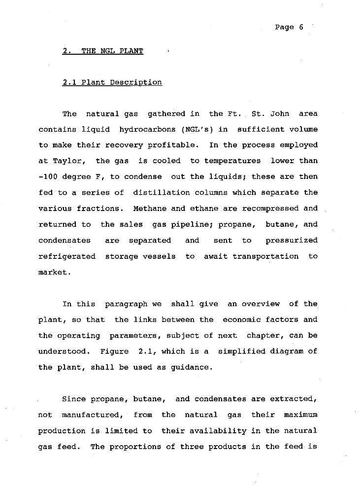
2. THE NGL PLANT ,
2.1 Plant Description
The natural gas gathered in the Ft. St. John area
contains liquid hydrocarbons (NGL's) in sufficient volume
to make their recovery profitable. In the process employed
at Taylor, the gas is cooled to temperatures lower than
-100 degree F, to condense out the liquids; these are then
fed to a series of distillation columns which separate the
various fractions. Methane and ethane are recompressed and
returned to the sales gas pipeline; propane, butane, and
condensates are separated and sent to pressurized
refrigerated storage vessels to await transportation to
market.
In this paragraph we shall give an overview of the
plant, so that the links between the economic factors and
the operating parameters, subject of next chapter, can be
understood. Figure 2.1, which is a simplified diagram of
the plant, shall be used as guidance.
Since propane, butane, and condensates are extracted,
not manufactured, from the natural gas their maximum
production is limited to their availability in the natural
gas feed. The proportions of three products in the feed is

Figure 2.1 Taylor Natural Gas Liquid Plant Concytual Schematic
Page 7
.........................................
i RAW GAS i
Jc ( MACMAHON GAS PLANT 1
.....
LPG removal efficiency here is dictated by flowrate and influences
........................ . composition is dependent on which wells are producing
lquality of sweet gas
PLANT ,;. side
residue gas must meet 2
minimum heat content specification
&
PIPELINE
t- by pass to PIPELINE
....................................... i NGL FEED j i GAS i
FILTER
to train 'B'
..... - ...............
rT-4 recovery efficiency is
v.. ..............
feedstock cost based on heat value removed by C C4 and C + produced 3' 5
IEXPANDERI mainly determined by
1 the operation of the
................................................................................................... POWER to flow and j
pressure ..................... ............................................................................. !..
I I I r e s i d u e g a s > PIPELINE ....................................................................................
FUEL to the i
1 FRACTIONATION ...............................................................................
I u C 4 butane
C5+ condensates
product mix and quantity are determined by :
-quantity & flow of feed gas . -recovery efficiency
-market requirements

Page 8
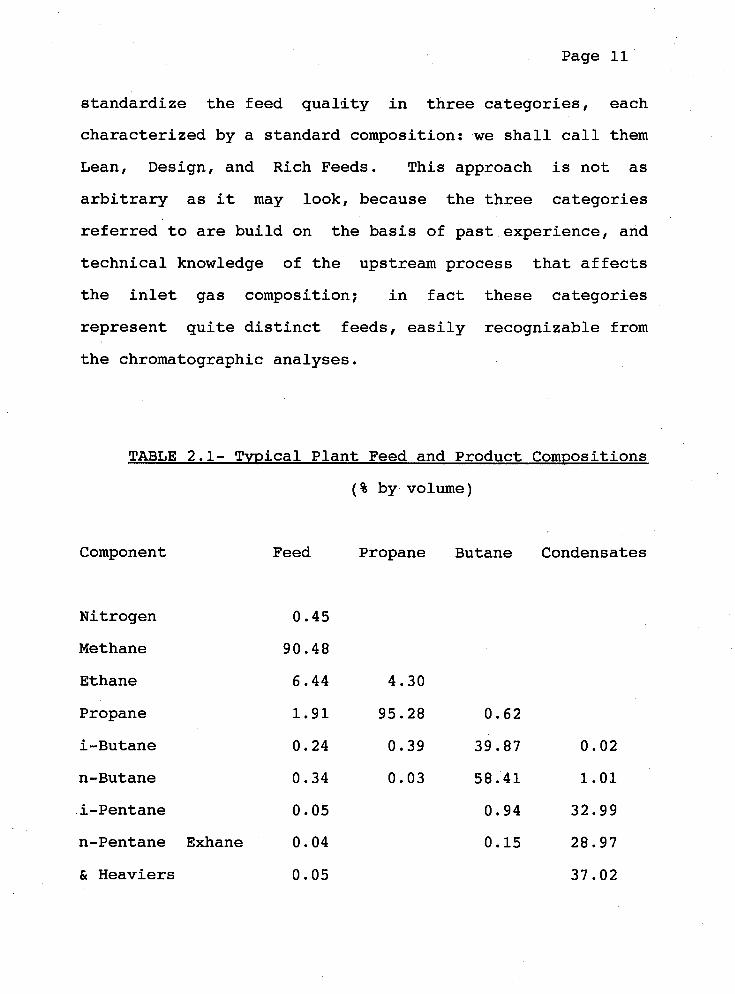
a given, and it varies, (within predictable limits)
independently of plant operations; seasonal variations are
typical, but fluctuations also happen on day-to-day basis,
mostly due to the fact that different wells produce gas
with different compositions (see table 2.1 for typical
compositions of feed gas and products).
Feed quantity can be varied at wish within the minimum
and maximum plant turndown. Since plant is made of two
production lines which can be operated either independently
or in parallel, overall flow can vary from a minimum of
about 150 millions of standard cubic feet per day (MMSCFD)
to a maximum of about 450 MMSCFD.
Recovery efficiency for propane can be adjusted by the
operator with wide ranges (about 65% minimum, to a maximum
of 95%); for butane and condensate it stays constant at
about 100%. Different recovery efficiencies are associated
with different costs; i.e. for the same production
quantities costs are different depending on whether a high
flow - low efficiency, or a low flow - high efficiency
combination is used. While there are ways of going behyond
these limits, they are technologically inefficient, and
shall not be considered,
Removing propane, butane, and condensates from the

Page 9
feed gas reduces the heat value of the latter, by an amount
proportional to the total amount of propane, butane, and
condensates extracted; this difference in heat value
between the feed and residue gas is the base for the cost
of the feedstock. Restated, cost of the feedstock is
directly proportional to the amounts of propane, butane,
and condensate produced, through a physical characteristic
of the products, which is their heat value.
Electric power is mainly used to run the compressors
that return methane and ethane to the pipeline. There is
one of such compressors for each production line. In first
approximation, recompression power is a linear function of
the feed flow. (Appendix A includes a regression analysis
performed with actual plant data, which confirms this
assumption is acceptable in the whole range of feed gas
flow) .
Natural gas supplies the heat needed for various
processes, and it is paid in proportion to its consumption.
There is storage available, which provides a buffer
between plant production and sales requirement; this is
used both to make operation smoother (since it is always
more desirable, from the technological point of view, to
operate at steady state than to fluctuate), and to take
Page 10
care of break-downs, equipment maintenance requirements,
and other events, that may reduce the plant availability,
either in a planned or unplanned way. Within the weekly
planning horizon, this means that some storage has to be
available to meet unexpected plant shut-downs, or
unexpected reduction of feed availailability. This problem
will be discussed later; it suffices for now to note that
it could be approached in different ways, such as
increasing the production during the first days of the week
(but this may prove disruptive, therefore more costly in
the long run), or by taking the chance (based on past
break-down experience) and not planning for it at all.
The products are shipped with both tank-cars and
trucks; propane is mostly shipped via rail,
As mentioned, the operator has no control on the
quality (i.e. composition) of the incoming flow; this does
not mean that the concentration of the products in the feed
is totally unpredictable, but it is certainly not possible
to know it exactly before it gets into the process and is
analyzed. Furthermore, the concentrations can
theoretically vary continuosly within a pretty wide range,
and life would become very complicated if some
simplification was not possible. The approach that will be
taken here is the same currently used at the plant, i.e. to
Page 11
standardize the feed quality in three categories, each
characterized by a standard composition: we shall call them
Lean, Design, and Rich Feeds. This approach is not as
arbitrary as it may look, because the three categories
referred to are build on the basis of past experience, and
technical knowledge of the upstream process that affects
the inlet gas composition; in fact these categories
represent quite distinct feeds, easily recognizable from
the chromatographic analyses.
TABLE 2.1- Typical Plant Feed and Product Compositions
( % by volume)
Component
Nitrogen
Methane
Ethane
Propane
i-Butane
n-Butane
i-Pentane
n-Pentane Exhane
& Heaviers
Feed Propane Butane Condensates

Page 12
2.2 Current Production Schedulinq System
Every monday morning a firm order for the shipment of
propane, butane, and condensates is posted by the Marketing
Dpt., to be filled by the plant before the end of the week.
Based on this, and on the estimated inlet composition, the
operators must decide on the flow amount and recovery level
to operate the plant. Other variables considered are: the
inventory level in hand, and the amount of products to keep
as ending inventory for the week. Forecast of future
weekly orders are available from the annual and quarterly
budgets, periodically adjusted on the basis of marketing
information.

Page 13
3 . COSTS AND REVENUES1
3.1 Introduction
In the following paragraph we shall review the
relationship between some of the variables the operator has
control on, and the cost and revenues associated with plant
operation. We shall first define the process variables,
then review their costs; lastly, we will briefly look at
the revenues, and their implications.
To meet the production target, the operator shall
adjust a number of physical variables (like pressures,
temperature, flows, etc.), There are hundreds of these
variables; for the purpose of this study, they will be
aggregated in two macroscopic factors that can easily be
related to plant production, and profit. They are:
natural gas feed flow, or gas throughput, which is the
amount of natural gas processed at the plant; and propane
recovery efficiency, that is the overall measure of how
much of the propane contained in the feed is actually
extracted.
From the point of view of these variables, when the
operator is given a certain target production, he can
choose to operate at maximum throughput and to limit the
Page 14
recovery efficiency, to run at maximum efficiency and
reduced throughput, or to work at any intermediate
condition between these extremes.
In addition to marketing requirements, there may be
other situations, plant specific, that may force the
operator to work at one set of conditions instead of
another. Storage level is one of the major constraints.
As a consequence of operator's decision (i.e. his choice of
flow and propane recovery level), and of the particular
condition of the feed, the plant will use a certain amount
of feed, will produce a certain product mix (revenue
generating), and will require certain amounts of energy (in
the form of electric power, and fuel gas).
We shall review and explain the relationship between
these variables and the cost or revenues associated with
them.
3.2 Process Variables
Natural gas feed flow is the amount of gas that is
taken from the pipeline (see fig. 2.1) to be processed,
and from which to extract propane, butane, and condensates.
It is an independent variable that the operator can
control, and it can be adjusted at virtually any value

Page 15
between 150 and 450 MMSCFD.
Feed composition is predictable, but it cannot be
controlled; it is a characteristic of the gas available,
and is subject to daily and seasonal variations.
Composition is continuously monitored, so propane, butane,
and condensate content of the feed is known, and the
operator can do some adjustments to operation during a run.
Propane recovery efficiency is the ratio between the
amount of propane recovered, and the amount contained in
the feed. It is the macroscopic measurable effect of a
certain combination of pressures, temperatures, and flows
at various points in the plant; it is a convenient
reference dimension that captures the effect of numerous
variables. It is continuosly monitored but its control can
only be done indirectly by adjusting the combination of
several operating parameters. It is possible to obtain the
same efficiency with different sets of operating
parameters, but operator's experience, and plant
instrumentation will lead to the choice of the most
efficient combination.
As indicated before, recovery efficiencies for the v 11
other two products (butane and condensates) is constant
(100%) because of the thermodynamic of the process.

Page 16
Electric power is mostly used to run the two
compressors which return the residual methane and ethane to
the pipeline. Each one of those compressors may use up to
8500 KW; the actual requirement depends on gas flow,
pressure, temperature, and composition on one hand, and
machine efficiency on the other. On average, power
requirement is a linear function of gas flow, within the
practical range of plant conditions. Appendix A.2 contains
the regression of actual plant data.
Fuel gas has a variety of uses, ranging from heat
generation (i.e. boilers) to process functions. Its usage
depends on a number of factors, and is mostly related to
production rate (see Appendix). It can be seen from
operating records that fuel consumption is small, and its
cost is a minor component of the total cost (table 3.1).
Products are sold by volume (cubic meters) and have to
meet certain composition specifications. The plant may
occasionally produce off-spec products which are
temporarily stored, then re-processed. There are certainly
costs associated with these re-runs, but the quantities
involved are definitely minimal in a well run, new plant
like the Taylor facilities, and in first approximation it
is safe to disregard those costs.

3.3 Costs
Page 17
We shall now review each of the items that make-up the
plant operating cost, and explain the structure of each one
of them; we shall refer to table 3.1 which is a typical
cost break-down for a plant similar to the Taylor NGL.
Operating Personnel. Unless the plant is shut-down
for maintenance, the number of people required for its L
operation does not change with level of production. This
cost is available from the annual budget.
Property Taxes. They are assessed periodically and
remain fixed over the budget period.
Insurance. Premiums are fixed over the budget period,
even though they are subject to periodic re-assessment and
neqociations.
Depreciation. It is presently calculated on
straight-line, 30 year basis, and its value can be taken
from the accounting records.
Maintenance. This cost is budgeted for a year and is
not strictly a fixed cost, since the equipment wear and
Page 18
tear is somehow dependent cm the level of usage. However,
an average maintenance costs may be used to cover the whole
range of plant operation without affecting the materiality
of the results.
Feed Gas. Feedstock cost is calculated by adding a
"demand charge" to a "commodity charge". The former is a
fixed cost, to be paid whether or not the gas is used; the ).
latter is a usage fee directly proportional to the amount
of heat content removed from the natural gas feed by the
extraction process; this is the heat value lost by the
natural gas due to the removal of propane, butane, and
condensate. The heat content of the unit of product is a
physical constant, therefore this cost can simply be
obtained by multiplying the measured (or projected)
quantity of each product by the respective constant.
Actual composition may vary slightly among production runs,
but with insignificant effect on the constant.
Power. The B.C. Hydro contract is structured in a
fashion similar to the feed gas shrinkage contract in that
there are a demand, and an energy charge. The demand
charge is the greater of:
- actual registered demand for the billing month; - contractual minimum demand;

- 75% of the highest ,during the previous
months.
After reviewing the power bills for the
Page 19
11 billing
past twelve
months, it was concluded that, in first approximation,
demand charge is a fixed cost. However, it must be
recognized that it is structured to give an incentive to
smooth operation of the plant and to avoid too high peaks
(e.g. run the plant for two periods at half capacity
instead of for one at full load).
Energy charge is a straight consumption charge, i.e.
it is proportional to the number of kilowatthour (kwh)
consumed during the billing month.
As mentioned earlier, power can be correlated with gas
flow through the plant, therefore its cost can be
calculated as a function of the gas flow.
Fuel. Fuel is taken from the pipeline and is paid on
a usage basis; it is metered and paid under the same
contract that covers the feed gas, and there is no demand
charge.
Marketing Fee. It is a fixed fee that is paid
annually to the Company that takes care of the marketing of

Page 20
the products; it is available from that contract.
Operating Fee. It is a contractual fee added to the
plant costs to cover head office, and other service cost.
It is a fixed percent of production and power costs.
3.4 Revenues
Revenues are generated by the sales of the three
products. Current market prices for these products are
3 3 3 about $60/m , $80/m , and $100/m , respectively, at plant gate. These values will be used to derive the profit
function, which is at the basis of the optimization model.

Page 21
TABLE 3.1 - Operatinq~ Cost Breakdown for a
Tvpical NGL Plant
a - For plant at full load: Fixed Costs 20%
Variable Costs 80%
b - For plant at minimum capacity:
Fixed Costs 40%
Variable Costs 60%
c - Fixed Costs: Operating & Maintenance 25.0%
Property Taxes 4.5%
Insurance ,5%
Depreciation 15.0%
General & Administration 25.0%
Shrinkage (demand charge) 25.0%
d - Variable Costs: Power (energy charge) 15.0%
Shrinkage (commodity charge) 67.0%
Fuel 3.0%
Operating and Marketing Fees 15.0%

4. MODELLING
Page 22
4.1 Problem Statement
Before we describe the approach to modelling, we
shall briefly review the major items that characterize the
problem. Schematically they are the following:
- Every Monday, at 8 AM, a weekly order comes in;
- Due to market demand, only propane needs to be
monitored; the other two products (butane and
condensate) are always produced at maximum
limit;
- Projections of future orders are available (for
the quarter, the year, and for the following few
weeks ) ;
- Given a weekly order, a daily schedule for the
next seven days is to be determined;
- There is always the possibility of down-times due
to unforeseable circumstances, and they have to
be taken in some account; typically, production
tends to be higher in the first few days of the
week;
- There is storage available which can be used as
cushion to meet targeted order quantities;
- The weekly order quantity may be adjusted if there

Page 23
is a significant ecbnomic incentive;
- Daily production level must be smoothed;
- There are two product lines, which allow a
throughput between 150 and 450 MMSCFD; propane
recovery efficiency can be varied between 60% and
96%; butane and condensates are recovered at 100%
all the times
We shall answer the following general questions:
1. For a given daily requirement, what is the best
operating setting at minimum cost, and how does it
affect the other relevant factors?
2. Given a weekly requirement, build a model to
determine daily production schedule to minimize
cost.
Additional questions are of the type: how many weeks
in advance should be considered; how to safeguard against
breakdowns; how to smooth power requirements; what is the
sensitivity of the various factors such as weekly order,
forecasted demand, etc.

4 . 2 The Model
Page 24
We shall answer those questions in two stages:
* First we will determine the daily production
schedule that best fits the constrains;
* Then we will determine how to meet that daily
schedule, while maximizing the profit.
In this work, the first stage problem was solved with
an LP model; the second one in an analytical way. More
specifically, the LP model allows us to determine the
optimum daily production schedule on the basis of
technological parameters (i.e. shipping requirements,
inventory levels, plant capacity, projected future demands,
etc.); once the daily schedule is determined, rules are
given to determine which combination of flow and recovery
efficiency to use to maximize prof it.
The profit function was developed analytically from
the information available on plant cost and revenues, and
on the physical and technological relationship between
feed and products.
The solution of the LP model was approached with both
Page 25
numerical and simple heuristic methods; a sensitivity
analysis was done on the constrains; and actual data from
the 1987 operating year were used to validate the model.
The following paragraphs will first explore the
development of the profit function, its limitations, and
the consequences of its particular structure on the LP
formulation. The LP formulation and solution, with
objective function, constraints, and both numerical and
simple heuristic solutions will be presented later.
Lastly, the sensitivity of the model will be reviewed,
together with a discussion on extreme-case situations, and
ways to approach them.

Page 26
5. THE PROFIT FUNCTION
5.1 The Function and Its Analvsis
When the cost items and revenues listed in chapter 3
are analyzed, it becomes clear that each of them can be
expressed as a function of two variables: F, the natural
gas feed flow to NGL plant; and Qp, the amount of propane
to be produced (the amounts of butane and condensate
produced are proportional to the flow). Therefore, profit
G can be written as:
where A, B, C are constants.
This equation recognizes that profit is proportional
to the amount of propane produced (first term), to that of
butane and condensate produced (second term), and that
there are fixed costs to be covered (i.e. C, which is a
negative term). Coefficients A, B, C can be regressed from
past data, or calculated from the actual costs and revenues
(see following S 5 . 2 ) .
In addition, if we base our discussion on a given feed
composition, the amount of propane Qp produced can be

expressed as
Page 27
where E is the propane recovery efficiency, and k is a
proportionality constant which depends on propane
concentration in the feed.
Both F and E are constrained by plant design between
two extreme values, i.e.
and
therefore, it is also
where - Qmin - k * Emin * Fmin
and - Qmax - * Emax * Fmax
Equations [3], 141, and [5] define the boundaries of
the region of feasible operation, which is represented as
the shadowed area in figure 5.1.

Page 28

Page 29
Since the amount of )propane Qp to be produced is
given, equation [I] says that, within the feasibility
region, we achieve maximum profit when we operate at
maximum flow. By looking at figure 5.1 we see that this
optimal relationship between Qp, F, and E is given by the
line segments AB and BC; i.e. to produce between Qmin and
Qmax we are better off operating along those segments than
in any other point of the feasibility region. We shall
call ABC the operating line, and it is on that line that we
must operate at all times to maximize profit.
If we concentrate our attention on the points located
on the operating line, i,e. if we limit our discussion to
the points of maximum profit, we observe the following two
situations:
1) When %in < Qp < Q*
we have Qp = k * Emin * F with Fmin < < Fmax
therefore: F = Qp / (k*Emin)
and G = [A+B/(k*Emin)] * Qp + C [6]
2) When Q* < Qp < Qmax
we have = Fmax

Page 30
therefore: G = A *'Qp + B * Fmax + C E71
Since B, k, and E are all positive, it must be that
which means that the slope of the function G=G(Qp) is * *
greater at Qp c Q than at Qp > Q , as shown in figure 5.2. In other words, along the operating line G is an
increasing piece-wise linear concave function of Qp.
Concavity of the profit function implies that marginal * *
profit is higher at Q,<Q than at Qp>Q , and this
conclusion has a very important consequence for our
optimization model: it allows us to say that we shall try *
to avoid Qp>Q , and that to do so we must smooth production levels. We can see this better if we consider the
following.
Let us refer to figure 5.2 and let us assume that we
have to produce an amount Qp. We can do that operating one
day at Q1 and another day at Q2, hence generating a profit
G1+G2, but we could also produce Ql+q one day, and QZ-q the
other day generating a profit G3+G4. It is evident that
G3+G4>G1+G2 because the slope of AB is greather than the t
slope of BC. Thus, if we minimize deviations in daily
production levels we also maximize profit. Recalling what

Page 31

Page 32
we said in S 3 . 3 about the way electric power is priced, we
see that by smoothing daily production we also minimize
power cost.
To determine a production schedule that minimizes
daily fluctuations we shall use an LP model.
5.2 Comparison with Actual Runs
Note: Due to the confidential nature of cost and
revenue data, all units of measurement have been omitted
from the formulations, as well as from the a11 numerical
examples.
Data from 1987 production were collected to validate
the formulation presented in the previous section.
Coefficients A, B I and C in equation [l] were calculated
from the data on current contracts and average prices for
1987, The estimated profit function is:
where :
E = .65 for 150 < F < 450, and
.65 < E < .95 for . F = 450

Page 33
It is interesting to note +that to avoid a loss situation
(i.e. G<O) the above equation requires F to be always
greather than 297. Recalling that each production line can
only process feed flows up to 225 MMSCFD, the practical
meaning of [8] is that the plant operates at a profit only
when propane sales are high enough to need the operation of
both production units.
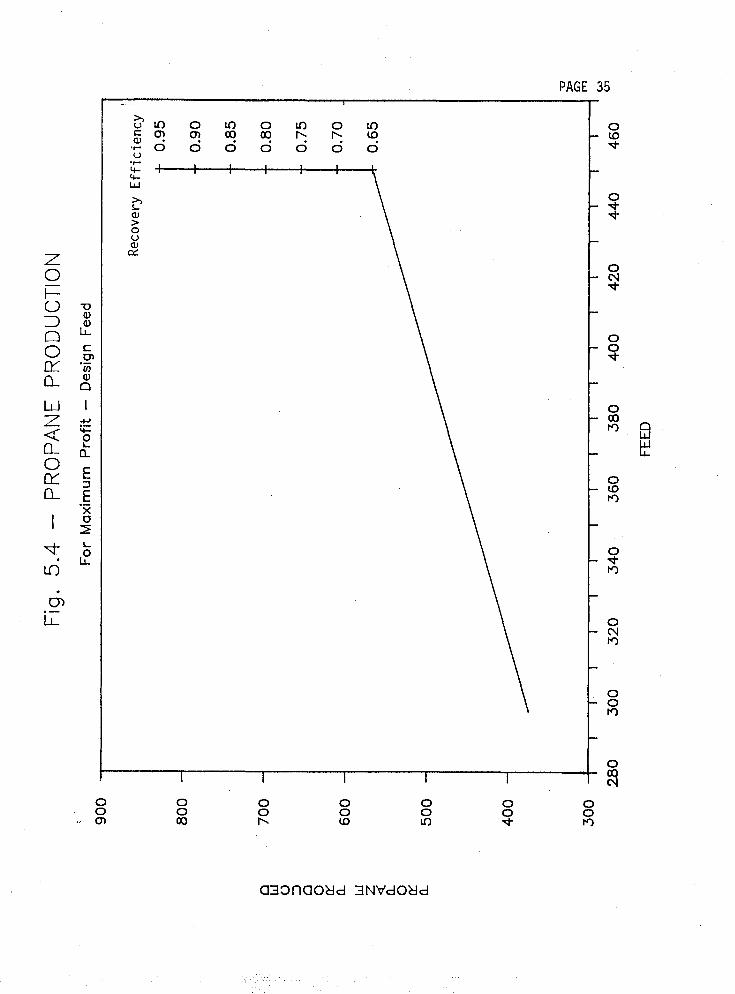
Using [8], the operating curves were determined for
three typical feed compositions, generally called Rich
(figure 5.3), Design (figure 5.4), and Lean (figure 5.5).
Once daily production level has been established (with the
LP model), these curves shall be used to determine the
optimum flow-recovery efficiency combination for the
available feed composition.
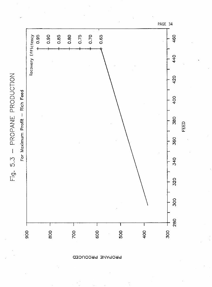
Fig.
5.3 -
PR
OP
AN
E P
RO
DU
CT
ION
For
Maxi
mum
Pro
fit - R
ich
Feed
Reco
very
Ef
fici
ency
280
300
320
340
360
380
400
420
440
460
FEE
D
PAGE 35

PAGE 36

Page 37
6. THE LP MODEL
6.1 LP Formulation
To develop the LP model, we need to define an
objective function, and a set of constraints. Based on the
characteristics of the profit function observed in •˜5.1),
our objective is to smooth the daily propane production
levels, for any given target production quantity over a
period of time, subject to the following workplace
constraints:
1- Sales requirement for the period must be met, i.e.
the sum of the daily shipments must equal the
sales target;
2- The maximum daily production cannot exceed maximum
plant capacity, for each given feed composition;
3- The maximum daily shipment cannot exceed the
capability of the loading bay. Since both
tank-cars and trucks are used, differences in the
two systems have to be taken into account.
4- Production, shipment, opening and closing
inventories have to be balanced;

Page 38
5- Storage capacity available cannot be exceeded.
A representation of the model is given in figure 6.1;
the constraints can be written as follows:
SUM (SHIPJi = SALES
(PROP)i < A
(SHIP)i < Bi
(CLINP)i-l + (PROP)i = (SHIP)i + (CLINP)i (CLINP)i < C
Where :
i = 1, 2, 3, ..., n = number of periods
considered;
SALES = target propane sales for the period;
(SHIP)i = shipment of product on day i;
propane production on day i;
(CLINP)i = closing propane inventory on day i =
= opening propane inventory on day i+l;
A = maximum daily propane production of the
plant; this value is set by plant design
and feed composition, and may be assumed
the same for all days of the week (about
830 units);

Page 39
Page 40
Bi = maximum propane shipment capacity for each
day (about 1300 units during week days,
and 100 units during weekends); tank cars,
which carry most of the propane, are not
loaded during weekends;
C = storage capacity available on site (about
1000 units).
6.2 O~enina and Closina Inventorv
Of the variables in the LP model, opening and closing
inventory levels require some detailed discussion, because
they link one period to the next, and influence future
decisions.
Inventory is a necessity for any operation, but it is
generally recognized as an unavoidable expense to be
minimized. In the case of Taylor NGL plant, costs
associated with on site storage are minimal compared to
other production costs and storage operating costs vary
very little with the amount of propane in the tanks. On
the other hand it may be useful to maintain a certain
inventory level, because it helps smoothing operation in
the next period. Therefore we cannot disregard the needs
for the optimization of the next period when looking at the
current one.

Page 41
To do this, we shalT approach optimization in two
steps: first, given the sales forecast for next period, we
shall determine the optimum opening inventory for that
period, which is also the closing inventory for the current
period; then, since we know the inventory in hand, we can
calculate daily production and shipping rates for the
current period.
The overall procedure to optimize plant operation
can be summarized in the following steps:
Based on the next period sales forecast, determine
the optimum (or desirable) closing inventory for
the current period;
Based on inventory in hand, and desirable closing
inventory for this period, determine the daily
production schedule;
Once the daily schedule is established, the
operating line (Figures 5.3, 5.4, 5.5) is used to
choose the combination of flow and recovery
efficiency that maximizes profit.
When the constraints, expressed in general terms in
S6.1, are examined in detail, we observe that the physical

Page 42
limitations of the plant I tend to somewhat simplify our
problem. Specifically, daily shipments have an upper
limit which is the same for all weekdays, and another
(lower) for the week-ends. This is due to the fact that
tank cars are only loaded during weekdays, and that
loading rate is limited by design.
In fact, only a minimum amount of loading is possible
during weekends (about 100 units per day) compared with
weekdays (about 1300 units). Given that daily propane
production has a maximum at about 830 units (constrained
by plant design and feed composition) we see that we can
ship more than the daily production in the first five days
of the week, while most of the weekend production goes to
storage.
Maximum storage is limited to the physical dimensions
of the tanks at the plant, and it would be impractical (and
very expensive) to either add storage, or to provide
storage offsite.
6.3 Heuristic Solution
Due to the special structure of the LP model, its
solution can be obtained by simple heuristics.
Specifically, let us assume that (by looking at next

Page 43
period sales forecast) we8 have defined that this week
closing inventory must be CLINP7 = 600, and that we have
in hand an inventory CLINPO = 754. Knowing that this week
sales is SALES = 4200, what is the optimum (i.e. the
smoothest) production schedule?
We know that maximum shipment is the following for
each day of the week (starting Monday): 1300, 1300, 1300,
1300, 1300, 100, 100; we also know that maximum inventory
is 1000. Smoothest operation, obviously, is the one that
requires the same production every day; in our case that
can be written in the following way:
(CLINP7 - CLINPO + SALES)/7=
= (600 - 754 + 4200)/7 = 4046/7 = 578
This, clearly, is not feasible, because if we produced
578 on both day 6 and 7, given that we can only ship 100 on
each of those days, we would end up with a volume in
storage of at least:
CLINP7 = 2 * 578 - 2 * 100 = 956
which is in excess of what we want. We shall then approach
the problem differently.

Page 44
Best schedule (in terms of smoothing) for weekends is
to start with empty inventory, i.e. with CLINP5 = 0, and
operate in the same fashion both on day 6 and 7. This
allows to produce more on those constrained days, and to
bring their production level closer to that of the less
constrained ones. Then:
The amount to be produced during the remaining five
days can now be calculated, given that the optimum is
"equal production each day". Therefore:
(SALES - PROP6 - PROP7) / 5 = 3400 / 5 = 680
We now have two questions to answer: is the solution
actually feasible (i.e. does it fit all the constraints);
and, can the solution be improved.
That the proposed solution is feasible is shown in the
following table 6.1:

Page 45
Table 6.1 - Heuristic Solution of LP
Can this solution be improved, i.e. is there a
production level between 578 and 680 for the weekdays, and
between 578 ands 400 for the weekends, that is feasible?
The answer is no, because we cannot produce any more during
the weekend; if we did, the closing inventory level would
be too high.
Let us now describe the general procedure for
determining the solution for a general problem, subject to
our particular set of constraints.
Step 1: Establish Feasibility. To do this, sales and

Page 46
production must be less than both the following values:
a) Max weekly sales =
= CLINPO + MAX WEEKDAY PRODUCTION + WEEKEND SHIPMENT =
= CLINPO + 832 * 5 + 200
b) Max weekly production =
= 832 * 5 + [CLINP7 - CLINPO + 2001
Step 2: Establish Weekend Production. This shall be
done assuming:
Step 3: Establish Weekdays Production. This shall be
done assuming:
PROPl=PROP2=PROP3=PROP4=PROP5, and CLINP5=O
Step 4: Check if Solution Can Be Improved. This shall
be done by relaxing any of the constraints, keeping in mind
that absolute optimum (i.e. the one with no constraints) is
"same production level every day of the week",
The following are two example based on the above

sequence.
Page 47
Example 1
Requirements: SALES=5000; CLINPO=200; CLINP7=800
Solution: MAX SALES = 200 + 832 * 5 + 200 =
= 4560 < 5000
Therefore, no feasible solution exists.
Example 2
Requirements: SALES=4200; CLINPO=450; CLINP7=500
Solution: MAX SALES = 450 + 832 * 5 + 200 =
= 4810 > 4200 OK
MAX PRODUCTION = 832 * 5 + 200 + 500 - 450 =
PRODUCTION REQUIRED = 4200 + 500 - 450 =
= 4250 < 4410 OK
Therefore, a feasible solution exists, and we could
try the following one:
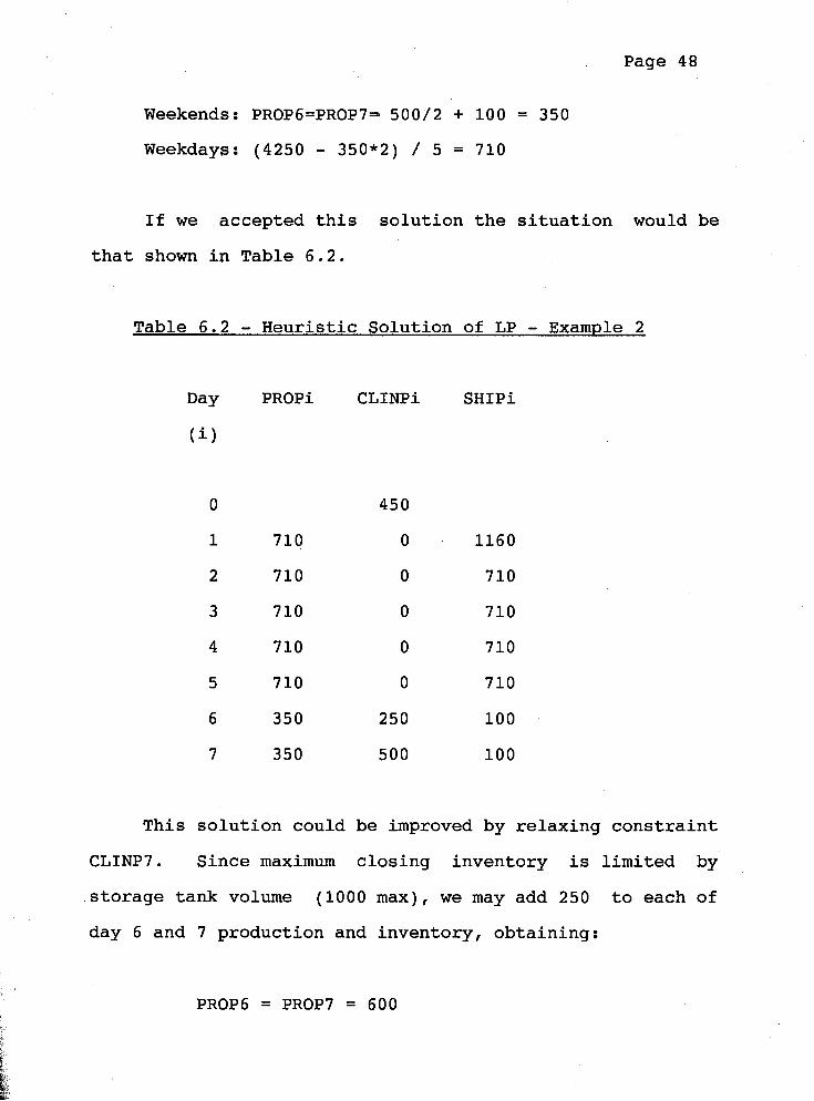
Weekends: PROP6=PROP7= 500/2 + 100 = 350
Weekdays: (4250 - 350*2) / 5 = 710
Page 48
be If we accepted this solution the situation would
that shown in Table 6.2.
Table 6.2 - Heuristic Solution of LP - Example 2
This solution could be improved by relaxing constra
CLINP7. Since maximum closing inventory is limited
storage tank volume (1000 max), we may add 250 to each
day 6 and 7 production and inventory, obtaining:
int
by
of
Page 49
and reducing weekday production to
Clearly this is a better solution for this period, if
the requirement for opening inventory of next period can be
relaxed.
Page 50
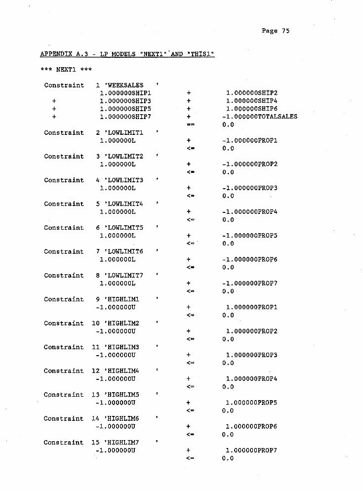
7 . THE LP SOLUTION ,
For the actual computer runs two LPts were used: one
(called "NEXT") to determine this period best closing
inventory, on the base of next period requirements; the
other (called "THIS") to determine the current period
production schedule. The basic difference between the two
is in the way opening and closing inventories are
constrained. For the actual formulation, the period chosen
was the current week, since that is the way orders are
taken at the plant. Obviously, the equations can be easily
adapted to periods of different lenght. The meaning of
each equation is explained here, and they are all shown in
tables 7.1 and 7.2 (note that it is always i=1,2,...,7
except where otherwise indicated).
Objective Function PRODELTA:
Min U - L To impose that production levels be as even as
possible, the objective function was set-up to
minimize the difference between maximum and minimum
daily production during the period under
consideration. U and L are the upper and lower
limits, respectively, of the daily productions during
the period.

Page 51
Constraint WEEKSALES: I
SUM(SHIPi) - TOTALSALES = O
It establishes that total weekly demand (TOTALSALES)
has to be satisfied by the total daily shipments
( SHIPi ) ;
Constraints LOWLIMITit
They calculate the smallest among the daily
productions (PROPi) and assign that value to the
dummy variable L;
Constraints HIGHLIMi :
They calculate the largest among the daily
productions (PROPi) and assign that value to the
dummy variable U;
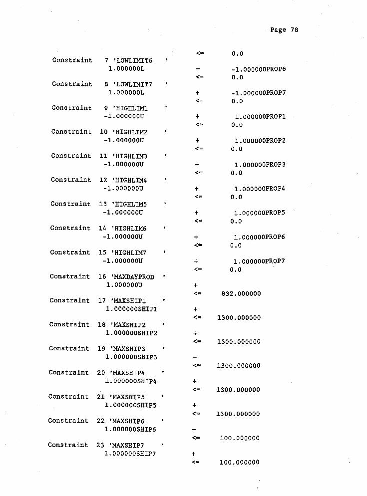
Constraint MAXDAYPRD:
U =< 832
This imposes an upper limit to the daily production,
In the way it is written it implies that maximum
production is the same every day; it can be expanded
and rewritten for every day, if different limits have
to be imposed;

Page 52
Constraints MAXSHIPi: I
These impose limitations on the maximum daily
shipments;
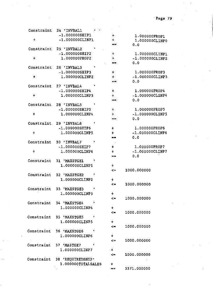
Constraints INVB&Lir
CLINPi - + PROPi - SHIPi - CLINPi = 0
These are the inventory balance equations, that
equate production (PROPi), inventory on hand
(CLINPi), and shipment (SHIPi). The opening balance
of the first day of the week, which is the same as
the closing balance of the previous week, is called
CLINPO ;
Constraints MAXSTGEi:
Maximum storage available is the volume of the
storage spheres, and is imposed with these equations;
Constraint REQUIREDSHIP:
TOTALSALES = weekly requirement
This constraint sets the sales amount for next
week;

Page 53
(From this point on the equation for the two LP models,
NEXT and THIS, are different).
NEXT - Constraint LOOP: CLINPO - CLINP7 = 0
NEXT is used to take into account next week
production to calculate the optimum closing inventory
for this week. To do that, as explained in $36.2,
this constraint imposes that opening and closing
inventory for next week are the same.
THIS - Constraint CLOSINV7: CLINP7 = as determined from "NEXT"
Since the (desirable) closing inventory for this week
is now known, this equation imposes its value;
THIS - Constraint CLINPOFIX: CLINPO = as known at scheduling time
This equation sets the opening inventory for this
week, as actually existent at the plant.

Page 54
Table 7.1 - Equations'for Model NEXT MIN U - L S.T. SUM(SHIPi) - TOTALSALES = 0 (i=lr2, ..., 7)
CLINPO - CLINP7 = 0
TOTALSALES = weekly requirement
Table 7.2 - Equations for Model THIS MIN U - L S.T. SUM(SHIPi) - TOTALSALES = 0 (i=lr2,. *,7)
CLINPi =< 1000
CLINP7 = as determined from "NEXT"
CLINPO = as known at scheduling time
TOTALSALES = weekly requirement

Page 55
8. COMPARISON WITH ACTUAL OPERATION
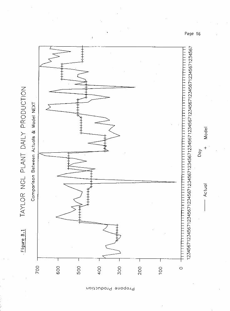
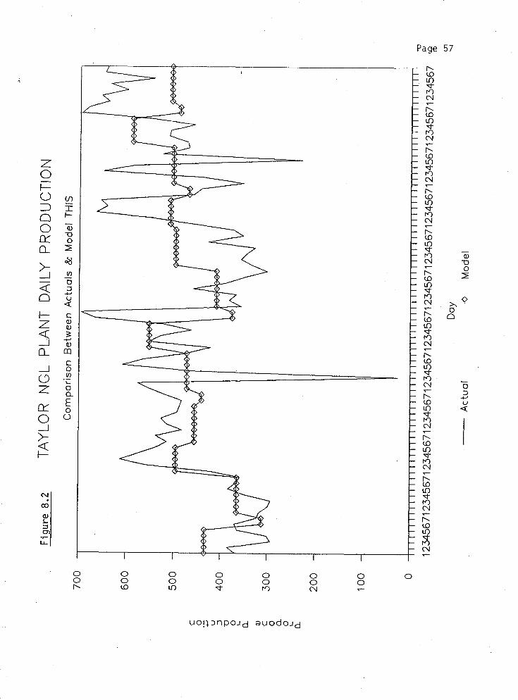
8.1 Model Plannina vs. Actual
The LP's presented above were tested against a
period of twelve weeks for which production data were
available. For each week the model NEXT was used first,
and its results applied to the model THIS; details of the
results are included in Appendix. Figures 8.1 and 8.2 show
the difference between the actual production and the ones
that would have been targeted for if the model had been
used: clearly, the model produces a much smoother
operation. The model clearly gives superior results even
taking into account that it gives target volumes, which
will actually vary because of fluctuations in the
operating parameters and, mostly, in the composition of
the feed. The weekly fluctuations were zero (i.e. same
production level every day) for six weeks; more
importantly, the target production level changed only ten
times during the twelve weeks, as opposed to about fourty
actual major changes (without taking into account the minor
daily variation that could never be eliminated anyway).
I Page
Page 57
Page 58
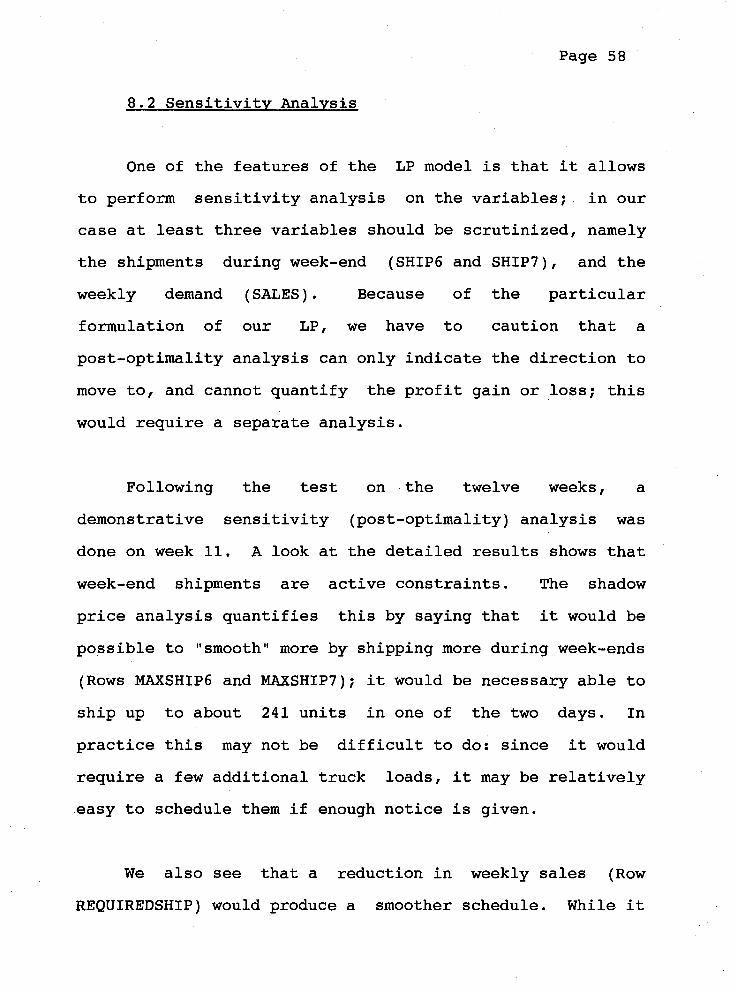
8.2 Sensitivity Analysis
One of the features of the LP model is that it allows
to perform sensitivity analysis on the variables; in our
case at least three variables should be scrutinized, namely
the shipments during week-end (SHIP6 and SHIP7), and the
weekly demand (SALES). Because of the particular
formulation of our LP, we have to caution that a
post-optimality analysis can only indicate the direction to
move to, and cannot quantify the profit gain or loss; this
would require a separate analysis.
Following the test on the twelve weeks, a
demonstrative sensitivity (post-optimality) analysis was
done on week 11. A look at the detailed results shows that
week-end shipments are active constraints. The shadow
price analysis quantifies this by saying that it would be
possible to "smooth" more by shipping more during week-ends
(Rows MAXSHIP6 and MAXSHIP7); it would be necessary able to
ship up to about 241 units in one of the two days. In
practice this may not be difficult to do: since it would
require a few additional truck loads, it may be relatively
easy to schedule them if enough notice is given.
We also see that a reduction in weekly sales (Row
REQUIREDSHIP) would produce a smoother schedule. While it
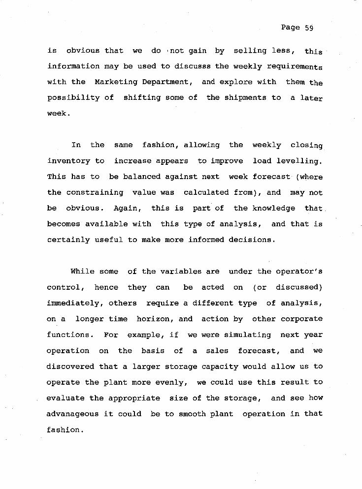
is obvious that we do lnot gain by selling less, this
information may be used to discusss the weekly requirements
with the Marketing Department, and explore with them the
possibility of shifting some of the shipments to a later
week.
In the same fashion, allowing the weekly closing
inventory to increase appears to improve load levelling.
This has to be balanced against next week forecast (where
the constraining value was calculated from), and may not
be obvious. Again, this is part of the knowledge that
becomes available with this type of analysis, and that is
certainly useful to make more informed decisions.
While some of the variables are under the operatorrs
control, hence they can be acted on (or discussed)
immediately, others require a different type of analysis,
on a longer time horizon, and action by other corporate
functions. For example, if we were simulating next year
operation on the basis of a sales forecast, and we
discovered that a larger storage capacity would allow us to
operate the plant more evenly, we could use this result to
evaluate the appropriate size of the storage, and see how
advanageous it could be to smooth plant operation in that
fashion.

Page 60
8.3 Special Cases t
Lastly, we shall briefly discuss two subjects that
may interfere or limit the applicability ~f the LP based
scheduling. We refer to the potential need to handle
contingencies (like equipment break-downs), and to the
case when just one of the two production lines may be
sufficient to satisfy demand.
Let us start with the problem of the two parallel
lines, and of how to decide whether to use one or two lines
to make a required production. Figure 8.3 shows the choice
available at each propane production level; we see that
between 180 and 360 units, one line is the only choice;
between 360 and 430 units it is possible to operate either
one or two lines; over 430 units two lines must be
operated, So there are legitimate reasons to check whether
one or two lines should be used for producing between 360
and 430 units.
One way of looking at the problem is to say that, as
shown in section 5.2, there is a minimum flow corresponding
to zero profit, and that flow is above the maximum capacity
of one line. Therefore, if there are not enough orders to
require more than that capacity, it is not profitable to
fill them. Whether this means a total plant shutdown is

Page 6 1

Page 62
still to be seen, and decided case by case. From a more
general point of view, we can say that the Marketing
Department is responsible to look after the sales, to
insure enough contracts are in place to take care of the
plant capacity.
For what concerns contingencies that may arise during
the week, while the production plan is in progress, current
practice is either to have a minimum storage, or to make
proportionally more production at the beginning of the
week; the choice being dictated by contingent factors (e.g.
inventory levels) or by operators perception of the
situation (e.g. type and number of problems experienced in
the recent past). Following the same approach, and given
that the future cannot be predicted very accurately, we can
disregard contingencies for what concerns the LP model, and
leave adjustements to the operator. The sensitivity
analysis provided by the LP model is going to supplement
the operating experience (which cannot be modelled), and
the operator is going to decide what to do with daily
production. We believe this is a better approach than
manipulating the constrains (e.g. by restricting some of
the daily outputs to imply less-than-maximum capacity)
because it provides the operator with the appropriate
information, but leaves the decision to his judgement.
Page 63
9. CONCLUSIONS ,
It was demonstrated that an LP model could be used to
determine optimum propane daily production levels to be
used to plan the weekly production. The procedure was
tested against twelve weeks of actual plant data, and the
results have shown that significant improvements in plant
operation can be achieved by using the model. The next
logical step is to actually use the model in the plant.
This will be attempted soon, and is planned to take
place in the following steps:
- Plant management will be presented with the model,
its basis, its logic, so that any controversial
aspect can be discussed and clarified.
- The senior operators will be involved, the
objectives and the practical aspects of the model
will be discussed with them, and a starting date
will be decided.
- For about four weeks, the model will be used to
determine target production levels, without
actually using the results for production
scheduling. This allows for "de-bugging", any

Page 64
adjustment to the I local conditions, as well as
familiarization of the operators with the use of
the program.
- Actual (i.e. operator set schedules) shall be
compared with model predictions, to confirm that
these are feasible and acceptable. Post optimality
analyses shall be performed to determine influence
of the various factors.
- If the previous stage confirms the practicality,
and the applicability of the model, and once
operator acceptance and confidence has been gained,
the model will be used to actually plan weekly
production on a steady basis. When appropriate,
post optimality analyses shall be run, and results
discussed.
- After sufficient data have been collected, it may
be that the model has to be adjusted or modified.
Post optimality analyses shall be performed on the
trends, to determine the actual value of the
bottlenecks.
As mentioned in the introduction, this is the first
attempt to model plant production at Taylor with a

Page 65
matematical tool like LP I programming; as any first, it
probably is a rough approximation of the reality, and
refinements will be required. However, we hope that the
first step is a good one, capable of giving a small but
useful hand to increase profitability of Taylor Plant.

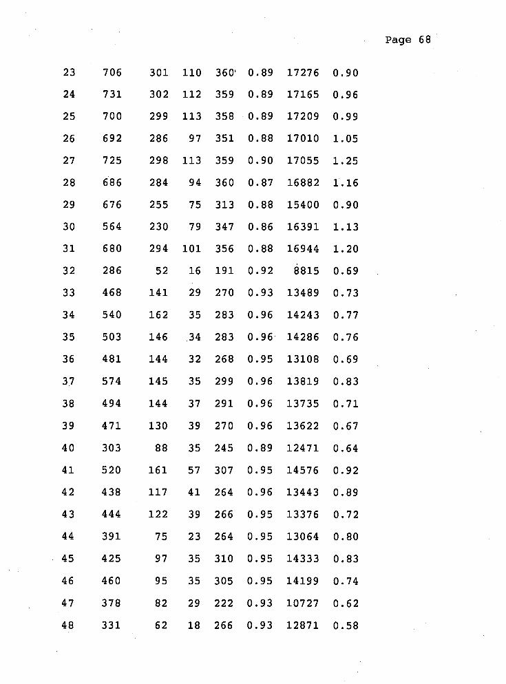
Page 66
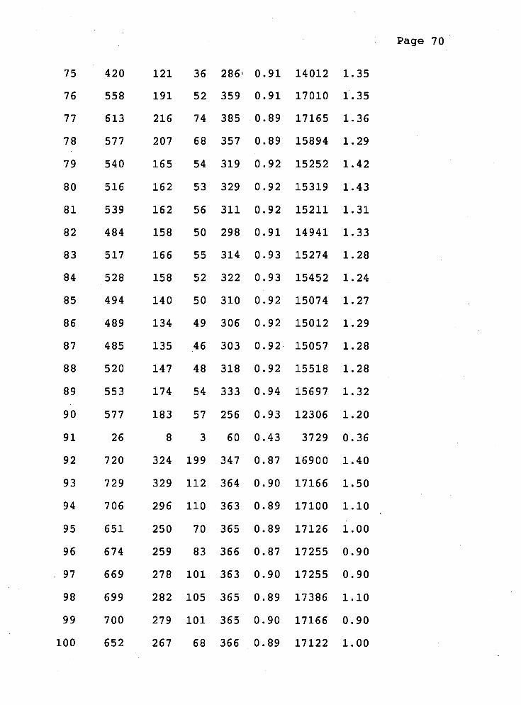
APPENDIX A.l - PRODUC'lIBN DATA
The following tables compile 120 days of production
data collected between June 1987 and February 1988, used
for the statistical analysis of Appendix A.2.
Each row contains data from one day production;
variables have the following meaning (units of measurement
have purposely been omitted due to the confidentiality of
the information):
PROPANE Propane produced
BUTANE Butane produced
COND Condensate produced
FEED Feed gas to the plant
C3REC Propane recovery efficiency
PWR Total recompression power
FGNET Net fuel gas consumption

Page 67
PRODUCTION DATA '
PROPANE BUTANE COND FEED C3REC PWR FGNET
Page 68

Page 69
Page 70

Page 71

Page 72
APPENDIX A.2 - RECOMPRESSION POWER REGRESSION ANALYSIS
The following pages contain the regression analysis
done on recompression power (PWR) using data from Appendix
A.1, and FEED (Plant feed gas flow) as the independent
variable. The results show a very high correlation between
2 the two variables, as well as a high significance of R . Figure A.l is a plot of the data, and of the regression
line. The estimated equation is:
PWR = 1471 + 42.84 * FEED

Page 73

Page 74
**** Multiple Regression Report ****
Dependent Variable: PWR
Independent Parameter Stndized Standard t-value Prob. Simple
Variable Estimate Estimate Error (b-0) Level R-Sqr
Intercept 1471.016 0.0000 404.3427 3.64 0.0004
FEED 42.84189 0.9477 1.327724 32.27 0.0000 0.8982
**** Analysis of Variance Report ****
Dependent Variable: PWR
Source
Constant
Model
Error
Total
df Sums of Squares Mean Square F-Ratio Prob. Level
(Sequential)
1 2.408761EtlO 2.408761EtlO
1 1.081511Et09 1.081511Et09 1041.17 0.000
118 1.225719Et08 1038745
119 1.204083Et09 1.011834Et07
Root Mean Square Error 1019.189
Mean of Dependent Variable 14167.92
Coefficient of Variation 7.1936333-02
R Squared
Adjusted R Squared
Page 75
Constraint
t t t
Constraint
Constraint
Constraint
Constraint
Constraint
Constraint
Constraint
Constraint
Constraint
Constraint
Constraint
Constraint
Constraint
Constraint
1 'WEEKSALES ' 1.000000SHIP1 1.000000SHIP3 1.000000SHIP5 1.000000SHIP7

Page 76
Constraint 16 'MAXDAYPROD ' ' 1.000000u
Constraint
Constraint
Constraint
Constraint
Constraint
Constraint
Constraint
Constraint
t
Constraint
t
Constraint
t
Constraint
t
Constraint
t
Constraint
t
Constraint
t

Page 77
constraint
Constraint
Constraint
Constraint
Constraint
Constraint
Constraint
Constraint
Constraint
31 'MAXSTGEl 9
1.000000CLINPl
32 'MAXSTGE2 9
1.000000CLINP2
33 'MAXSTGE3 9
1.000000CLINP3
34 'MAXSTGE4 9
1.000000CLINP4
35 'MAXSTGE5 t
1.000000CLINP5
36 'MAXSTGE6 v
1.000000CLINP6
37 'MASTGE7 9
1,000000CLINP7
38 'LOOP 9
1.000000CLINPO
39 'REQUIREDSHIP' 1.000000TOTALSALES
Objective function (PRODNDELTA ) to be MINimised 1.000000U t -1.000000L ---- =---- ---- ----
*** THIS1 *** Constraint
Constraint
Constraint
Constraint
Constraint
Constraint
1 'WEEKSALES ' 1.000000SHIP1 1.000000SHIP3 1,000000SHIP5
Page 78
Constraint
Constraint
Constraint
Constraint
Constraint
Constraint
Constraint
Constraint
Constraint
Constraint
Constraint
Constraint
9 'HIGHLIMI -1.000000U
10 'HIGHLIMP -1.oooooou
13 'HIGHLIMS -1.000000u
16 'MAXDAYPROD 1.000000u
Constraint 19 'MAXSHIP3 t
1.000000SHIP3
Constraint 20 'MAXSHIP4 t
1.000000SHIP4
Constraint 21 'MAXSHIP5 ' 1.000000SHIP5
Constraint 22 'MAXSHIP6 ' 1.000000SHIP6
Constraint 23 'MAXSHIP7 ' 1.000000SHIP7
Page 79
Constraint
t
Constraint
+ Constraint
t
Constraint
t
Constraint
t
Constraint
t
Constraint
t
Constraint
Constraint
Constraint
Constraint
Constraint
Constraint
Constraint
Constraint 38 'REQUIREDSHIP' 1.000000TOTALSALES

Page 80
Constraint 39 'closinv7s ' ' 1.000000CLINP7 t
== 424.571000 Constraint 40 'CLINPOFIX '
1.000000CLINPO t 31 1000~000000
Objective function (PRODNDELTA ) to be MINimised 1.000000u t -1.000000L

Page 81
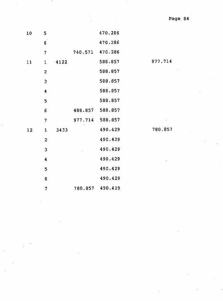
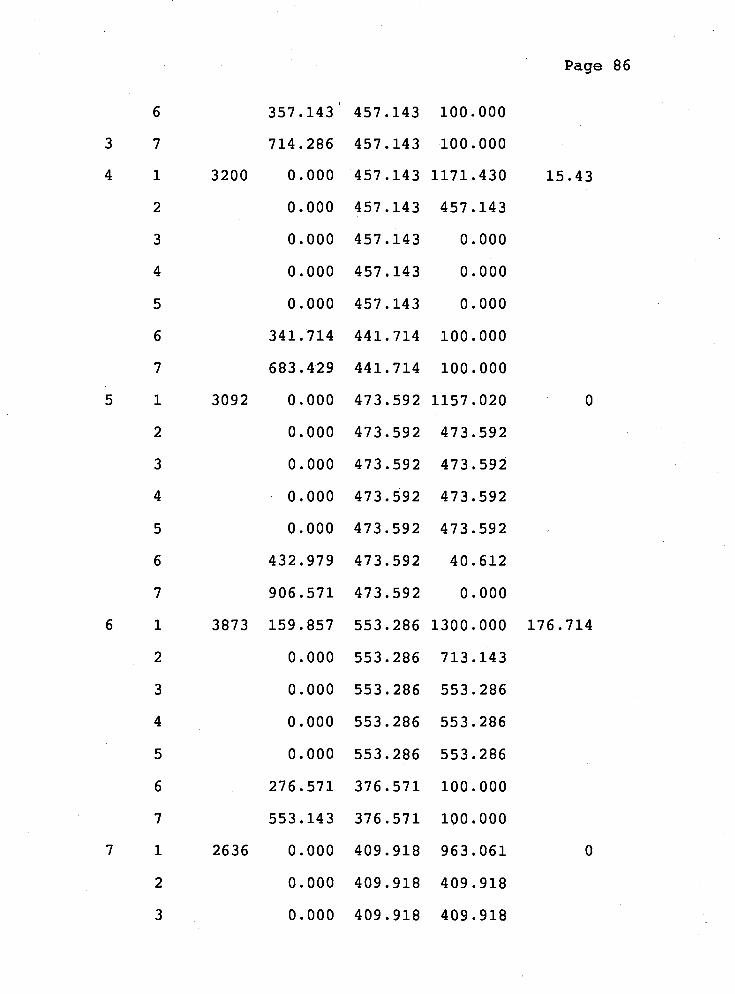
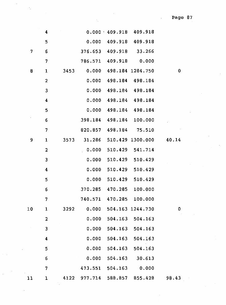
APPENDIX A.4 - SUMMARY OF RESULTS FROM MODEL "NEXT" FOR TWELVE WEEKS
Each period is calculated imposing CLINPO=CLINP7; the
calculated (CLINPO)i is then used as (CLINP7)i-l for the
"THISi" runs.

Page 82

Page 8 3
Page 84

Page 85
APPENDIX A.5 - SUMMARY OF RESULTS FROM MODEL "THIS"
...................................................... ......................................................
WEEK DAY SALES CLINP PROP SHIP U-L
...................................................... ......................................................
0 - - 1000 - - - - - -
1 1 3371 865.800 434.200 568.400 121.915
2 0.000 434.200 1300.000
Page 86
Page 87

Page 88

Page 89
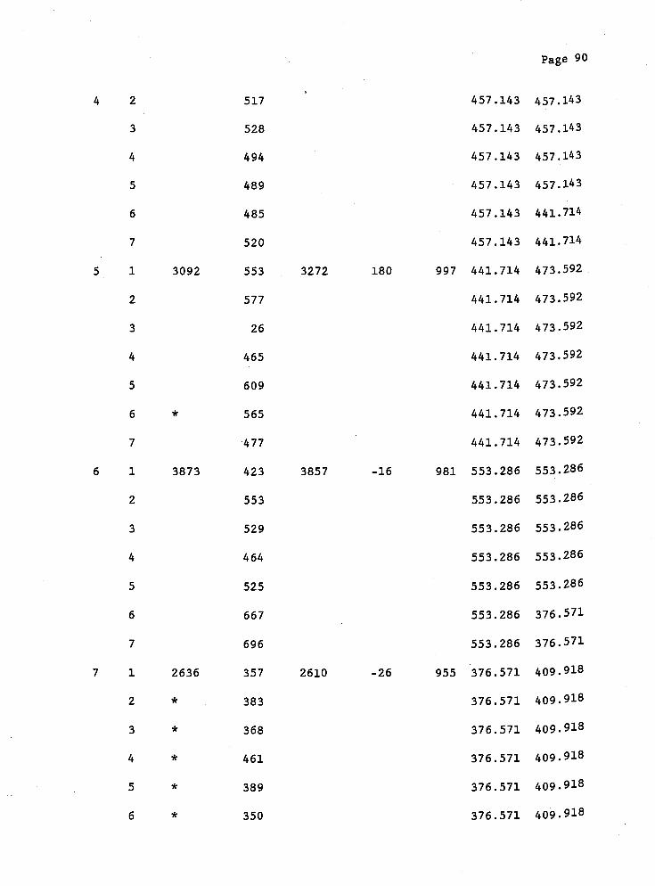
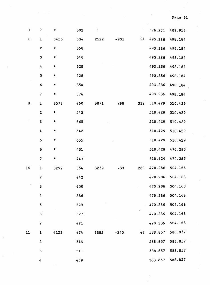
APPENDIX A.6 - COMPARISON BETWEEN ACTUALS AND MODEL RESULTS -P--P---------=~-------=I=====I=====================~============~~~====
WK DAY SALES ACTUAL ACTUAL DELTA INV NEXT THIS
DAILY WKLY SALES 1000
1 1 3371 368 2404 -967 33 434.200
2 385 434,200
3 293 434.200
4 301 434.200
5 364 434.200
6 370 312.285
7 323 312.285
2 1 2186 317 2366 180 213 312.860 364.939
Page 90
Page 91

Page 92

Page 93
APPENDIX A.7 - POST-OPTIMALITY ANALYSIS FOR CASE "THIS11"
MINIMUM solution basis
' SHIP1 t
's1k:LOWLIMIT'
's1k:LOWLIMIT'
's1k:LOWLIMIT'
's1k:LOWLIMIT'
' PROP7 9
' L '
' PROP 6 9
' PROP1 9
' SHIP2 9
' SHIP3 '
' SHIP4 t
's1k:LOWLIMIT'
's1k:HIGHLIMG'
'slk:HIGHLIM7'
' u '
' PROP2 '
' PROP3 9
'slk:MAXSHIP3'
' slk:MAXSHIP4 '

Page 94
"s1k:MAXSHIPS '
' SHIP6 9
' SHIP7 '
' CLINPO 9
' CLINP1 9
's1k:MAXDAYPR'
' PROP4 '
's1k:MAXSHIPl'
' SHIP5 9
' CLINP6 9
's1k:MAXSTGEl'
'slk:MAXSTGE2'
'slk:MAXSTGE3'
'slk:MAXSTGE4'
'slk:MAXSTGE5'
's1k:MAXSTGEG'
'slk:MASTGE7 '
' PROP5 '
'CLINP7 '
' TOTALSALES '
MINIMUM value of the function 'PRODNDELTA '

Page 95
=== SHADOW PRICE ANALYSIS ===
=Ll=fPI=EP==========I========I=
= CONSTRAINING ROWS =
NUMBER ROW
WEEKSALES
LOWLIMIT6
LOWLIMIT7
HIGHLIMl
HIGHLIMB
HIGHLIM3
HIGHLIM4
HIGHLIM5
MAXSHIP6
MAXSHIP7
INVBALl
INVBALZ
INVBAL3
INVBAL4
INVBAL5
INVBAL6
INVBAL7
SHADOW PRICE LOWER LIMIT
REQUIREDSHIP0.200000
closinv7s -.500000
CLINPOFIX -.200000
UPPER LIMIT
UNITS 1111.43
UNITS 196.857
UNITS 196.857
UNITS 492.143
UNITS 492.143
UNITS 492.143
UNITS 492.143
UNITS 492.144
UNITS 240.612
UNITS 240.612
UNITS 1215.71
UNITS 361.071
UNITS 736.071
UNITS 736.071
UNITS 736.071
UNITS 196.857
UNITS 196.857
UNITS 5233.43
UNITS
UNITS
UNITS
UNITS
UNITS
UNITS
UNITS
UNITS
UNITS
UNITS
UNITS
UNITS
UNITS
UNITS
UNITS
UNITS
UNITS
UNITS
0.1705303-12 UNITS 977.714 UNITS
0.0 UNITS 1469.86 UNITS
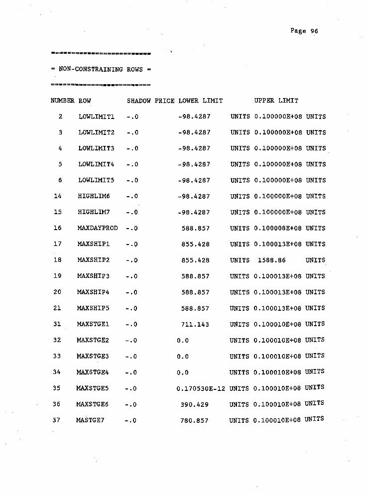
Page 96
-- --I=====a===1=1========z= I
= NON-CONSTRAINING ROWS =
==P==a==IPP3P=~=5t==~OI==
NUMBER ROW
LOWLIMIT1
LOWLIMIT2
LOWLIMIT3
LOWLIMIT4
LOWLIMITS
HIGHLIM6
HIGHLIM7
MAXDAY PROD
MAXSHIPl
MAXSHIP2
MAXSHIP3
MAXSHIP4
MAXSHIPS
MAXSTGEl
MAXSTGE2
MAXSTGE3
MAXSTGE4
MAXSTGES
MAXSTGE6
MASTGE7
SHADOW
-.o
-.o
-. 0 -.o
-.o
-, 0
-.o
-.o
-.o
-.o
-.O
-.o
-.o
-.o
-. 0 -.o
-.o
-.O
- ,o -.o
PRICE LOWER LIMIT UPPER LIMIT
-98.4287 UNITS 0~100000Et08 UNITS
-98.4287 UNITS 0~100000Et08 UNITS
-98 4287 UNITS 0~100000Et08 UNITS
-98.4287 UNITS 0~100000Et08 UNITS
-98.4287 UNITS 0~100000Et08 UNITS
-98.4287 UNITS 0~100000Et08 UNITS
-98.4287 UNITS 0~100000Et08 UNITS
588.857 UNITS 0.100008Et08 UNITS
855.428 UNITS 0.100013Et08 UNITS
855.428 UNITS 1588.86 UNITS
588.857 UNITS 0.100013Et08 UNITS
588.857 UNITS 0.100013Et08 UNITS
588.857 UNITS 0.100013Et08 UNITS
711.143 UNITS 0.100010Et08 UNITS
0.0 UNITS 0.100010Et08 UNITS
0.0 UNITS 0.100010Et08 UNITS
0.0 UNITS 0.100010Et08 UNITS
0.1705303-12 UNITS 0.100010Et08 UNITS
390.429 UNITS 0.100010Et08 UNITS
780.857 UNITS 0.100010Et08 UNITS

Page 97
NON-BASIC VARIABLE OBJECTIVE CHANGE (VALUE) VALID UP TO
X( 19) 'CLIBP2 ' -0.0 288.857 units
X( 20) 'CLINP3 ' -0.0 588.857 units
X( 21) 'CLINP4 ' -0.0 588.857 units
X( 22) 'CLINP5 ' -0.700000 736.071 units
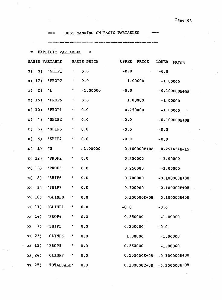
Page 98
=== COST RANGING ON'BASIC VARIABLES
---3-------3-------====EEE====EEfE=E==~P=E=E==
= EXPLICIT VARIABLES =
BASIS VARIABLE BASIS PRICE UPPER PRICE LOWER PRICE
' SHIP1 '
' PROP7 '
' L '
' PROP6 '
' PROP1 '
' SHIP2 '
' SHIP3 9
' SHIP4 9
' U '
' PROP2 '
' PROP3 '
' SHIP6 '
' SHIP7 '
'CLINPO '
'CLINP1 '
' PROP4 '
' SHIP5 '
'CLINP6 '
' PROP5 '
'CLINP7 '
'TOTALSALE'
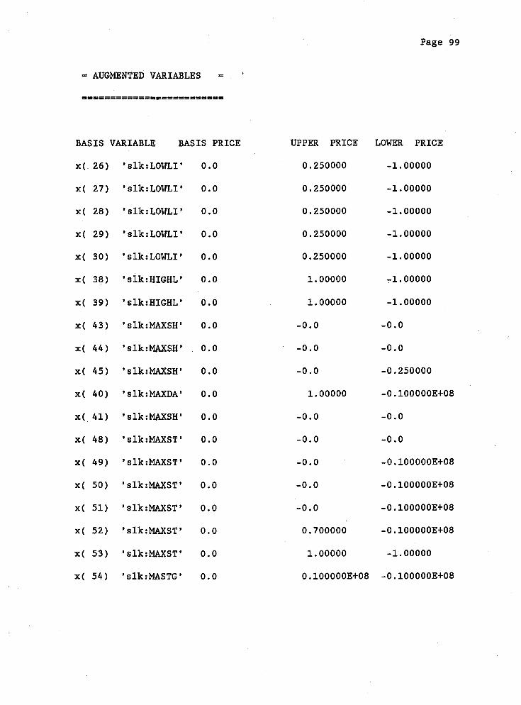
Page 99
- AUGMENTED VARIABLES = '
==t======P==S-IPP=====PPs
BASIS VARIABLE BASIS PRICE UPPER PRICE
O.25OOOO
O.25OOOO
O.25OOOO
O.25OOOO
O.25OOOO
1.00000
1.00000
-0.0
-0.0
-0.0
1.00000
-0.0
-0.0
-0.0
-0.0
-0.0
O.7OOOOO
1.00000
LOWER PRICE
-1.00000
-1.00000
-1.00000
-1.00000
-1.00000
-1.00000
-1.00000
-0.0
-0.0
-O.25OOOO
-0~100000E+08
-0.0
-0.0
-0.100000Et08
-0.100000Et08
-0.100000Et08
-0~100000Et08
-1.00000
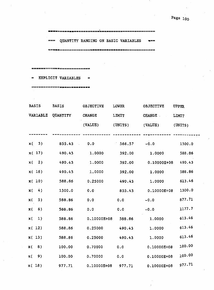
BASIS
VARIABLE
BAS IS
QUANTITY
OBJECTIVE
CHANGE
( VALUE )
LOWER OBJECTIVE UPPER
LIMIT CHANGE LIMIT
(UNITS) ( VALUE ) (UNITS )

Page 101
711.14 0.0 ' 266.57 -0.0 1000.0

Page 102
BASIS
QUANTITY
98.429
98.429
98.429
98.429
98.429
98.429
98.429
711.14
711.14
711.14
243.14
444.57
288.86
1000.0
1000.0
1000.0
1000.0
609.57
219.14
OBJECTIVE
CHANGE
( VALUE )
0.25000
0.25000
O.25OOO
O.25OOO
O.25OOO
1.0000
1.0000
0.0
0.0
0.0
1.0000
0.0
0.0
0.0
0.0
0.0
O.7OOOO
1.0000
0.10000Et08
LOWER
LIMIT
(UNITS)
0.0
0.0
0.0
0.0
0.0
0.0
0.0
422.29
122.29
122.29
218.54
0.0
0.0
711.14
411.14
411.14
263.93
511.14
219.14
OBJECTIVE
CHANGE
(VALUE )
1.0000
1.0000
1.0000
1.0000
1.0000
1.0000
1.0000
-0.0
-0.0
O.25OOO
UPPER
LIMIT
(UNITS)
Related Documents