Natural frequencies, modes and critical speeds of axially moving Timoshenko beams with different boundary conditions You-Qi Tang a , Li-Qun Chen a,b, , Xiao-Dong Yang c a Shanghai Institute of Applied Mathematics and Mechanics, Shanghai 200072, China b Department of Mechanics, Shanghai University, 99 Shang Da Road, Shanghai 200436, China c Department of Engineering Mechanics, Shenyang Institute of Aeronautical Engineering, Shenyang 110136, China article info Article history: Received 14 May 2008 Received in revised form 27 August 2008 Accepted 14 September 2008 Available online 19 September 2008 Keywords: Axially moving beams Timoshenko model The complex mode approach Modes Natural frequencies Critical speeds abstract In this paper, natural frequencies, modes and critical speeds of axially moving beams on different supports are analyzed based on Timoshenko model. The governing differential equation of motion is derived from Newton’s second law. The expressions for various boundary conditions are established based on the balance of forces. The complex mode approach is performed. The transverse vibration modes and the natural frequencies are investigated for the beams on different supports. The effects of some parameters, such as axially moving speed, the moment of inertia, and the shear deformation, are examined, respectively, as other parameters are fixed. Some numerical examples are presented to demonstrate the comparisons of natural frequencies for four beam models, namely, Timoshenko model, Rayleigh model, Shear model and Euler–Bernoulli model. Finally, the critical speeds for different boundary conditions are determined and numerically investigated. & 2008 Elsevier Ltd. All rights reserved. 1. Introduction Axially moving beams are involved in many engineering devices, such as band saws, aerial cableways, power transmission chains, and serpentine belts. These systems suffer from the occurrence of transverse vibrations due to initial excitations. Transverse vibrations of these devices have been investigated to avoid possible resulting fatigue, failure and low quality. For example, the vibration of the blade of band saws causes poor cutting quality. The vibration of the belt leads to noise and accelerated wear of the belt in belt drive systems. Therefore, vibration analysis of axially moving beams is important for the design of the devices. There are many researches which have been carried out on axially moving systems in literatures. Mote [1] first investigated the effect of tension in an axially moving band and computed numerically the first three frequencies and modes for simply supported boundary conditions. Wickert and Mote [2] presented a classical vibration theory, comprised of a modal analysis and a Green’s function method, for the traveling string and the traveling beam where natural frequencies and modes associated with free vibration serve as a basis for analysis. O ¨ z and Pakdemirli [3,4] and O ¨ z [5] calculated the first two natural frequencies values for different flexural stiffnesses in the cases of pinned–pinned ends and clamped–clamped ends, respectively. Pakdemirli and Ulsoy [6] investigated the dynamic response of an axially accelerating string. O ¨ zkaya and Pakdemirli [7] considered transverse vibrations of an axially moving beam. O ¨ zkaya and O ¨ z [8] applied artificial neural networks to determine the natural frequencies of axially moving beams and gave a comparison of analytical and ANN results for natural frequency versus mean axial velocity in the first two modes. O ¨ z [9] investigated the transverse vibration of highly tensioned Euler–Bernoulli beams and computed natural frequen- cies of an axially moving beam in contact with a small stationary mass under pinned–pinned or clamped–clamped boundary con- ditions. Kong and Parker [10] used a different perturbation method to find closed-form, approximate eigensolutions of axially moving beams with small bending stiffness and combined perturbation techniques for algebraic equations and the phase closure principle to derive closed-form approximate natural frequencies of an axially moving beam with small flexural stiffness. Ghayesh and Khadem [11] investigated free non-linear transverse vibration of an axially moving beam in which rotary inertia and temperature variation effects have been considered and gave natural frequency versus the mean velocity and rotary inertia, critical speed versus the rotary inertia and natural frequency versus the mean velocity and temperature for the first ARTICLE IN PRESS Contents lists available at ScienceDirect journal homepage: www.elsevier.com/locate/ijmecsci International Journal of Mechanical Sciences 0020-7403/$ - see front matter & 2008 Elsevier Ltd. All rights reserved. doi:10.1016/j.ijmecsci.2008.09.001 Corresponding author at: Department of Mechanics, Shanghai University, 99 Shang Da Road, Shanghai 200436, China. Tel.: +86 2166136905. E-mail address: [email protected] (L.-Q. Chen). International Journal of Mechanical Sciences 50 (2008) 1448–1458

Welcome message from author
This document is posted to help you gain knowledge. Please leave a comment to let me know what you think about it! Share it to your friends and learn new things together.
Transcript

ARTICLE IN PRESS
International Journal of Mechanical Sciences 50 (2008) 1448–1458
Contents lists available at ScienceDirect
International Journal of Mechanical Sciences
0020-74
doi:10.1
� Corr
Shang D
E-m
journal homepage: www.elsevier.com/locate/ijmecsci
Natural frequencies, modes and critical speeds of axially moving Timoshenkobeams with different boundary conditions
You-Qi Tang a, Li-Qun Chen a,b,�, Xiao-Dong Yang c
a Shanghai Institute of Applied Mathematics and Mechanics, Shanghai 200072, Chinab Department of Mechanics, Shanghai University, 99 Shang Da Road, Shanghai 200436, Chinac Department of Engineering Mechanics, Shenyang Institute of Aeronautical Engineering, Shenyang 110136, China
a r t i c l e i n f o
Article history:
Received 14 May 2008
Received in revised form
27 August 2008
Accepted 14 September 2008Available online 19 September 2008
Keywords:
Axially moving beams
Timoshenko model
The complex mode approach
Modes
Natural frequencies
Critical speeds
03/$ - see front matter & 2008 Elsevier Ltd. A
016/j.ijmecsci.2008.09.001
esponding author at: Department of Mechan
a Road, Shanghai 200436, China. Tel.: +86 21
ail address: [email protected] (L.-Q. Ch
a b s t r a c t
In this paper, natural frequencies, modes and critical speeds of axially moving beams on different
supports are analyzed based on Timoshenko model. The governing differential equation of motion is
derived from Newton’s second law. The expressions for various boundary conditions are established
based on the balance of forces. The complex mode approach is performed. The transverse vibration
modes and the natural frequencies are investigated for the beams on different supports. The effects of
some parameters, such as axially moving speed, the moment of inertia, and the shear deformation, are
examined, respectively, as other parameters are fixed. Some numerical examples are presented to
demonstrate the comparisons of natural frequencies for four beam models, namely, Timoshenko model,
Rayleigh model, Shear model and Euler–Bernoulli model. Finally, the critical speeds for different
boundary conditions are determined and numerically investigated.
& 2008 Elsevier Ltd. All rights reserved.
1. Introduction
Axially moving beams are involved in many engineeringdevices, such as band saws, aerial cableways, power transmissionchains, and serpentine belts. These systems suffer from theoccurrence of transverse vibrations due to initial excitations.Transverse vibrations of these devices have been investigated toavoid possible resulting fatigue, failure and low quality. Forexample, the vibration of the blade of band saws causes poorcutting quality. The vibration of the belt leads to noise andaccelerated wear of the belt in belt drive systems. Therefore,vibration analysis of axially moving beams is important for thedesign of the devices.
There are many researches which have been carried out onaxially moving systems in literatures. Mote [1] first investigatedthe effect of tension in an axially moving band and computednumerically the first three frequencies and modes for simplysupported boundary conditions. Wickert and Mote [2] presented aclassical vibration theory, comprised of a modal analysis and aGreen’s function method, for the traveling string and the travelingbeam where natural frequencies and modes associated with free
ll rights reserved.
ics, Shanghai University, 99
66136905.
en).
vibration serve as a basis for analysis. Oz and Pakdemirli [3,4] andOz [5] calculated the first two natural frequencies values fordifferent flexural stiffnesses in the cases of pinned–pinned endsand clamped–clamped ends, respectively. Pakdemirli and Ulsoy[6] investigated the dynamic response of an axially acceleratingstring. Ozkaya and Pakdemirli [7] considered transverse vibrationsof an axially moving beam. Ozkaya and Oz [8] applied artificialneural networks to determine the natural frequencies of axiallymoving beams and gave a comparison of analytical and ANNresults for natural frequency versus mean axial velocity in the firsttwo modes. Oz [9] investigated the transverse vibration of highlytensioned Euler–Bernoulli beams and computed natural frequen-cies of an axially moving beam in contact with a small stationarymass under pinned–pinned or clamped–clamped boundary con-ditions. Kong and Parker [10] used a different perturbationmethod to find closed-form, approximate eigensolutions of axiallymoving beams with small bending stiffness and combinedperturbation techniques for algebraic equations and the phaseclosure principle to derive closed-form approximate naturalfrequencies of an axially moving beam with small flexuralstiffness. Ghayesh and Khadem [11] investigated free non-lineartransverse vibration of an axially moving beam in which rotaryinertia and temperature variation effects have been consideredand gave natural frequency versus the mean velocity and rotaryinertia, critical speed versus the rotary inertia and naturalfrequency versus the mean velocity and temperature for the first

ARTICLE IN PRESS
Y.-Q. Tang et al. / International Journal of Mechanical Sciences 50 (2008) 1448–1458 1449
two modes, respectively. All of above literatures, either simplesupports or fixed supports is researched. Yang and Chen [12,13]studied axially moving elastic and viscoelastic beams on simplesupports with torsion springs and gave the first two frequenciesand modes. Lee and Jang [14] investigated the effects of thecontinuously incoming and outgoing semi-infinite beam parts onthe dynamic characteristics and stability of an axially movingbeam by using the spectral element method.
The axially moving beam has been traditionally represented bythe Euler–Bernoulli beam theory by assuming that the beam isrelatively thin as compared with its length. It appears that, to theauthors’ knowledge, there have been very few studies on theaxially moving beam for Timoshenko model. Simpson [15] wasprobably the first to derive the equations of motion for the movingthick beam on the basis of the Timoshenko beam theory, but nonumerical results were given and he did not consider the axialtension in their equations. Chonan [16] studied the steady-stateresponse of a moving Timoshenko beam by applying Laplacetransform method. Lee [17] used exact dynamic stiffness matrix instructural dynamics to provide very accurate solutions, whilereducing the number of degrees of freedom to resolve thecomputational and cost problems. Challamel [18] compared theTimoshenko model with shear model for stationary beams with-out axial translations. Seon and Timothy [19] presented the fulldevelopment and analysis of four models for stationary beams.
Wickert and Mote [2] determined the critical transport speedfor second-order model and four-order model at which divergenceinstability occurs. Lee and Mote [20] gave the critical transportspeeds for a simply supported beam and fixed supports from thetime-independent equilibrium balance of the linear equation.Their works were based on the Euler–Bernoulli beam theory. Theboundary conditions were formerly researched for simple sup-ports and fixed supports. In this paper, the critical speeds of aTimoshenko beam on different boundary conditions are investi-gated.
The present paper is organized as follows. Section 2 derives thegoverning equation of motion and different boundary conditions.Section 3 investigates the frequencies and modes with thecomplex mode approach. Section 4 compares natural frequenciesfor four models on simple supports and predicts the effects ofsome parameters. Section 5 determines and numerically investi-gates the critical speeds on different boundary conditions. Section6 ends the paper with concluding remarks.
2. The governing equation of motion
Uniform axially moving Timoshenko beams, with density r,cross-sectional area A, area moment of inertia of the cross-sectionabout neutral axis J, shape factor k, modulus of elasticity E, axialtension P, shearing modulus of the beam G, travels at constantaxial transport speed G between different boundary conditionsseparated by distance L. The bending vibration can be describedby two variables dependent on axial coordinate X and time T,namely, transverse displacement Y(X,T) and the angle of rotationof the cross-section C(X,T) due to the bending moment.
Because shear deformations are considered, angle y of thebeam depends not only on angle C but also on shear angle g:
yðX; TÞ ¼ cðX; TÞ � gðX; TÞ (1)
Bending moment M(X,T) and shear force Q(X,T) are related tothe corresponding deformations,
M ¼ EJc;X
Q ¼ M;X ¼AG
k ðc� yÞ ¼AG
k ðc� Y ;XÞ (2)
According to Newton’s second law, the coupled governingequations of motion are obtained
� Q ;X dX cos y� rAðY ;TT þ 2GY ;XT cos yþ G2Y ;XX cos yÞdX
þ P sin ydX ¼ 0rJc;TT �M;X þ Q ¼ 0 (3)
Substituting Eqs. (2) into (3) yields the governing equation forthe transverse displacement for axially moving Timoshenkobeams
rJ 1þkP
AGþkE
G
� �Y ;XXTT � EJ 1þ
kP
AG
� �Y ;XXXX þ PY ;XX
� rAðY ;TT þ 2GY ;XT þ G2Y ;XXÞ �r2Jk
GðY ;TTTT þG2Y ;XXTT
þ 2GY ;XTTT Þ þrEJk
Gð2GY ;XXXT þ G2Y ;XXXXÞ ¼ 0 (4)
The expressions for various boundary conditions can beestablished based on the balance of forces. The boundaryconditions on simple supports
YjX¼0 ¼ 0;YjX¼L ¼ 0; MjX¼0 ¼ 0;MjX¼L ¼ 0 (5)
The boundary conditions on fixed supports
YjX¼0 ¼ 0;YjX¼L ¼ 0; yjX¼0 ¼ 0; yjX¼L ¼ 0 (6)
The boundary conditions on simple supports with torsionsprings
YjX¼0 ¼ 0;YjX¼L ¼ 0; MjX¼0 � KyjX¼0 ¼ 0;MjX¼L þ KyjX¼L ¼ 0 (7)
At both ends, all quantities in Eqs. (5)–(7) can be expressed inthe spatial partial-derivatives of the transverse displacement.Details can be found in Appendix.
Introduce the dimensionless variables and parameters
y ¼Y
L; x ¼
X
L; t ¼ T
ffiffiffiffiffiffiffiffiffiffiffiP
rAL2
s; v ¼ G
ffiffiffiffiffiffiffirA
P
r; k1 ¼
kJE
GAL2,
k2 ¼kJP
GA2L2; k3 ¼
J
AL2; k4 ¼
EJ
PL2(8)
Dimensionless parameter k1 associated with k2 accounts for theeffects of shear distortion, k3 presents the effects of the rotaryinertia, and k4 denotes the stiffness of the beam.
Substituting Eqs. (8) into (4)–(7) yields the dimensionless form
y;tt þ 2vy;xt þ ðv2 � 1Þy;xx � ðk1 þ k2 þ k3 � k2v2Þy;xxtt
þ ðk1 þ k4 � k1v2Þy;xxxx þ k2ðy;tttt þ 2vy;xtttÞ � 2k1vy;xxxt ¼ 0, (9)
yjx¼0 ¼ 0; yjx¼1 ¼ 0; y;xxjx¼0 ¼ 0; y;xxjx¼1 ¼ 0 (10)
yjx¼0 ¼ 0; yjx¼1 ¼ 0; y;xjx¼0 ¼ 0; y;xjx¼1 ¼ 0 (11)
yjx¼0 ¼ 0; yjx¼1 ¼ 0; y;xxjx¼0 � ky;xjx¼0 ¼ 0; y;xxjx¼1 þ ky;xjx¼1 ¼ 0
(12)
where k ¼ mL. Lee and Jang proposed a set of governing equationsfor axially moving Euler–Bernoulli beams to account for themomentum transport through the both end boundaries [14]. Forthe transverse vibration, their equation differentiates from thetraditional one with an additional y,xxtt term. However, the presentinvestigation still adopts the traditional formulation. It should benoticed that Eq. (9) contains term y,xxtt. Therefore, the followinganalysis may be valid for models developed by Lee and Jang’sapproach.

ARTICLE IN PRESS
Y.-Q. Tang et al. / International Journal of Mechanical Sciences 50 (2008) 1448–14581450
3. The frequencies and the modes
3.1. Simple supports
The solution to Eq. (9) can be assumed as
yx; t ¼ fnðxÞeiont þ fnðxÞe
�iont (13)
where fn and on denote the nth mode function and naturalfrequency and over bar represent complex conjugate. SubstitutingEqs. (13) into (9) yields
k2fno4n � 2ik2vf0no3
n þ ½ðk1 þ k2 þ k3 � k2v2Þf00n � fn�o2n
þ 2ivðf0n � k1f000
nÞon þ ðv2 � 1Þf00n þ ðk1 þ k4 � k1v2Þ f0000n ¼ 0
(14)
The simple boundary conditions demand
fnð0Þ ¼ 0; fnð1Þ ¼ 0; ð0Þ ¼ 0; f00nð1Þ ¼ 0 (15)
The solution to ordinary differential equation (14) can beexpressed by
fnðxÞ ¼ C1nðeib1nx þ C2neib2nx þ C3neib3nx þ C4neib4nxÞ (16)
Substituting Eqs. (16) into (14) and (15), yields
ðk1 þ k4 � k1v2Þb4in � 2vk1onb
3in � ½ðk1 þ k2 þ k3 þ k2v2Þo2
n
þ ð1� v2Þ�b2in þ ð2k2vo3
n � 2vonÞbin þ k2o4n �o
2n ¼ 0 (17)
1 1 1 1
b21n b2
2n b23n b2
4n
eib1n eib2n eib3n eib4n
b21neib1n b2
2neib2n b23neib3n b2
4neib4n
0BBBB@
1CCCCA
1
C2n
C3n
C4n
0BBBB@
1CCCCAC1n ¼ 0 (18)
For the non-trivial solution of Eq. (18), the determinant of thecoefficient matrix must be zero.
½eiðb1nþb2nÞ þ eiðb3nþb4nÞ�ðb21n � b2
2nÞðb23n � b2
4nÞ
þ ½eiðb1nþb3nÞ þ eiðb2nþb4nÞ�ðb23n � b2
1nÞðb22n � b2
4nÞ
þ ½eiðb2nþb3nÞ þ eiðb1nþb4nÞ�ðb22n � b2
3nÞðb21n � b2
4nÞ ¼ 0 (19)
Using Eqs. (18) and (19), one can obtain the modal function ofthe simply supported beam as follows:
fðxÞ ¼ c1 eib1nx �ðb2
4n � b21nÞðe
ib3n � eib1n Þ
ðb24n � b2
2nÞðeib3n � eib2n Þ
eib2nx
(
10
8
6
4
2
0.5 1 1.5 2 2.5 3 3.5�
�1
k4 = 0.04
k4 = 0.16
k4 = 0.36
k4 = 0.64
k4 = 1
Fig. 1. The natural frequencies vs. axially moving speeds for
�ðb2
4n � b21nÞðe
ib2n � eib1n Þ
ðb24n � b2
3nÞðeib2n � eib3n Þ
eib3x
� 1�ðb2
4n � b21nÞðe
ib3n � eib1n Þ
ðb24n � b2
2nÞðeib3n � eib2n Þ
þðb2
4n � b21nÞðe
ib2n � eib1n Þ
ðb24n � b2
3nÞðeib2n � eib3n Þ
!eib4nx
)(20)
The nth eigenvalues bjn (j ¼ 1, 2, 3, 4) and the correspondingnatural frequencies can be calculated numerically. Fig. 1 presentsthe natural frequencies for the first and second modes, respec-tively. They have been found that the natural frequencies decreasewith the increasing the axially moving speeds. The exact values atwhich the first natural frequency vanishes are called the criticalspeeds and afterwards the system is unstable about the zeroequilibrium.
Let v ¼ 1 and k4 ¼ 1. Fig. 2 presents the modal functions for thefirst and second modes, respectively. The dashed lines denotethe real parts of the modal functions and the solid lines denote theimaginary part of the modal functions. It should be remarked thatneither the real nor the imaginary parts of the modal functions aresymmetric, although both the beam and the boundary conditionsare symmetric. The phenomenon caused by the axial transporta-tion has been observed in the case of the Euler–Bernoulli beam aswell [2,15]. Later, it will be demonstrated that the shapes becomemore unsymmetrical as the axial speed increases.
3.2. Fixed supports
The fixed boundary conditions demand
fnð0Þ ¼ 0; fnð1Þ ¼ 0; f0nð0Þ ¼ 0; f0nð1Þ ¼ 0 (21)
Substituting Eqs. (16) into (21) yields
1 1 1 1
b1n b2n b3n b4n
eib1n eib2n eib3n eib4n
b1neib1n b2neib2n b3neib3n b4neib4n
0BBBB@
1CCCCA
1
C2n
C3n
C4n
0BBBB@
1CCCCAC1n ¼ 0 (22)
For the non-trivial solution of Eq. (22), the determinant of thecoefficient matrix must be zero.
½eiðb1nþb2nÞ þ eiðb3nþb4nÞ�ðb1n � b2nÞðb3n � b4nÞ
þ ½eiðb1nþb3nÞ þ eiðb2nþb4nÞ�ðb3n � b1nÞðb2n � b4nÞ
þ ½eiðb2nþb3nÞ þ eiðb1nþb4nÞ�ðb2n � b3nÞðb1n � b4nÞ ¼ 0 (23)
�2
35
30
25
20
15
10
5
0.5 1 1.5 2 2.5 3�
k4 = 0.04
k4 = 0.16
k4 = 0.36
k4 = 0.64
k4 = 1
different k4: (a) the first mode and (b) the second mode.

ARTICLE IN PRESS
2.5
2
1.5
1
0.5
0
-0.5
-10 0.2 0.4 0.6 0.8 1
x
�1 �2
3
2
1
0
-1
-20 0.2 0.4 0.6 0.8 1
x
Re
Re
Im
Im
Fig. 2. The modal functions diagrams: (a) the first mode and (b) the second mode.
20
15
10
5
1 2 3 4 5� �
�1 �2
50
45
40
35
30
25
20
15
10
5
0.5 1 1.5 2 2.5 3
k4 = 0.04
k4 = 0.16
k4 = 0.36
k4 = 0.64
k4 = 1
k4 = 0.04
k4 = 0.16
k4 = 0.36
k4 = 0.64
k4 = 1
Fig. 3. The natural frequencies vs. axially moving speeds for different k4: (a) the first mode and (b) the second mode.
Y.-Q. Tang et al. / International Journal of Mechanical Sciences 50 (2008) 1448–1458 1451
Using Eqs. (22) and (23), one can obtain the modal function ofthe fixed supports as follows:
fnðxÞ ¼ c1 eib1nx �ðb4n � b1nÞðe
ib3n � eib1n Þ
ðb4n � b2nÞðeib3n � eib2n Þ
eib2nx �ðb4n � b1nÞðe
ib2n � eib1n Þ
ðb4n � b3nÞðeib2n � eib3n Þ
eib3nx
�
þ �1þðb4n � b1nÞðe
ib3n � eib1n Þ
ðb4n � b2nÞðeib3n � eib2n Þ
þðb4n � b1nÞðe
ib2n � eib1n Þ
ðb4n � b3nÞðeib2n � eib3n Þ
� �eib4nx
�(24)
1 1 1 1
b21n þ ikb1n b2
2n þ ikb2n b23n þ ikb3n b2
4n þ ikb4n
eib1n eib2n eib31n eib4n
ðb21n � ikb1nÞe
ib1n ðb22n � ikb2nÞe
ib2n ðb23n � ikb3nÞe
ib3n ðb24n � ikb4nÞe
ib4n
0BBBB@
1CCCCA
1
C2n
C3n
C4n
0BBBB@
1CCCCAC1n ¼ 0 (26)
Fig. 3 presents the natural frequencies for the first and secondmodes, respectively.
Let v ¼ 1 and k4 ¼ 1, Fig. 4 presents the modal functions forthe first and second modes, respectively. The dashed lines denotethe real parts of the modal functions and the solid lines denote theimaginaries part of the modal functions.
3.3. Simple supports with torsion springs
The boundary conditions of simple supports with torsionsprings demand
fnð0Þ ¼ 0; fnð1Þ ¼ 0; f00nð0Þ � kf0nð0Þ ¼ 0; f00nð1Þ þ kf0nð1Þ ¼ 0 (25)
Substituting Eq. (16) into (25), yields
For the non-trivial solution of Eq. (26), the determinant of thecoefficient matrix must be zero.
eiðb1nþb2nÞðb1n � b2nÞð�ikþ b1n þ b2nÞðb3n � b4nÞðikþ b3n þ b4nÞ
þ eiðb1nþb3nÞðb3n � b1nÞð�ikþ b3n þ b1nÞðb2n � b4nÞðikþ b2n þ b4nÞ

ARTICLE IN PRESS
1
0.5
0
-0.5
-1
-1.5
-2
-2.50 0.2 0.4 0.6 0.8 1
x x
�1
�2
Im
Im
Re
Re
3
2
1
0
-1
-2
-30 0.2 0.4 0.6 0.8 1
Fig. 4. The modal functions diagrams: (a) the first mode and (b) the second mode.
Y.-Q. Tang et al. / International Journal of Mechanical Sciences 50 (2008) 1448–14581452
þ eiðb1nþb4nÞðb2n � b3nÞðikþ b2n þ b3nÞðb1n � b4nÞð�ikþ b1n þ b4nÞ
þ eiðb2nþb3nÞðb2n � b3nÞð�ikþ b2n þ b3nÞðb1n � b4nÞðikþ b1n þ b4nÞ
þ eiðb2nþb4nÞðb3n � b1nÞðikþ b3n þ b1nÞðb2n � b4nÞð�ikþ b2n þ b4nÞ
þ eiðb3nþb4nÞðb1n � b2nÞðikþ b1n þ b2nÞðb3n � b4nÞð�ikþ b3n þ b4nÞ ¼ 0
(27)
Using Eqs. (26) and (27), one can obtain the modal function ofthe simple supports with torsion springs as follows:
fnðxÞ
¼ C eib1nx �ikðb1 � b3Þðb1 � b4Þðe
ib1 þ eib3 Þ þ ðb1 � b4Þðk2þ b3b4 þ b1b3 þ b1b4 þ b2
4Þðeib1 � eib3 Þ
ikðb2 � b3Þðb2 � b4Þðeib2 þ eib3 Þ þ ðb2 � b4Þðk
2þ b3b4 þ b2b3 þ b2b4 þ b2
4Þðeib2 � eib3 Þ
eib2nx
(
þikðb1 � b2Þðb1 � b4Þðe
ib1 þ eib2 Þ þ ðb1 � b4Þðk2þ b2b4 þ b1b2 þ b1b4 þ b2
4Þðeib1 � eib2 Þ
ikðb2 � b3Þðb3 � b4Þðeib2 þ eib3 Þ þ ðb3 � b4Þðk
2þ b3b4 þ b2b3 þ b2b4 þ b2
4Þðeib2 � eib3 Þ
eib3nx
� 1�ikðb1 � b3Þðb1 � b4Þðe
ib1 þ eib3 Þ þ ðb1 � b4Þðk2þ b3b4 þ b1b3 þ b1b4 þ b2
4Þðeib1 � eib3 Þ
ikðb2 � b3Þðb2 � b4Þðeib2 þ eib3 Þ þ ðb2 � b4Þðk
2þ b3b4 þ b2b3 þ b2b4 þ b2
4Þðeib2 � eib3 Þ
"
þikðb1 � b2Þðb1 � b4Þðe
ib1 þ eib2 Þ þ ðb1 � b4Þðk2þ b2b4 þ b1b2 þ b1b4 þ b2
4Þðeib1 � eib2 Þ
ikðb2 � b3Þðb3 � b4Þðeib2 þ eib3 Þ þ ðb3 � b4Þðk
2þ b3b4 þ b2b3 þ b2b4 þ b2
4Þðeib2 � eib3 Þ
#eib4nx
)(28)
Fig. 5 presents the natural frequencies for the first and secondmodes, respectively, for different spring stiffness values.
Let v ¼ 1, k4 ¼ 1 and k ¼ 200, Fig. 6 presents the modalfunctions for the first and second modes, respectively. The dashedlines denote the real parts of the modal functions and the solidlines denote the imaginaries part of the modal functions.
Fig. 7 presents the contribution of axially moving speeds tomodal functions. The dashed lines denote v ¼ 0.01, the dottedlines denote v ¼ 1 and the solid lines denote v ¼ 2. They havebeen found that the symmetry decrease with the increase inaxially moving speeds.
Fig. 8 presents the contribution of spring stiffness tomodal functions. The dotted lines denote k ¼ 2, the dashed linesdenote k ¼ 20 and the solid lines denote k ¼ 200. It has beenfound that the symmetry decreases with the increase in springstiffness.
Fig. 9 presents the contribution of shear modulus to modalfunctions. The solid lines denote G ¼ 66�109, the dashed linesdenote G ¼ 100�109 and the dotted lines denote G ¼ 200�109. Ithas been found that the symmetry decreases with the increase inspring stiffness.
4. The comparison of natural frequencies for four models onsimple supports
The linear governing equation of Euler model and boundarycondition are
y;tt þ 2vy;xt þ ðv2 � 1Þy;xx þ k4y;xxxx ¼ 0 (29)
fnð0Þ ¼ 0;fnð1Þ ¼ 0;f00nð0Þ ¼ 0;f00nð1Þ ¼ 0 (30)
Fig. 10 presents the natural frequencies for the first and secondmodes, respectively.
The linear governing equation of Rayleigh model and boundarycondition are
y;tt þ 2vy;xt þ ðv2 � 1Þy;xx � k3y;xxtt þ k4y;xxxx ¼ 0 (31)
fnð0Þ ¼ 0;fnð1Þ ¼ 0;f00nð0Þ ¼ 0;f00nð1Þ ¼ 0 (32)
Fig. 11 presents the natural frequencies for the first and secondmodes, respectively.
The linear governing equation of Shear model and boundarycondition are
y;tt þ 2vy;xt þ ðv2 � 1Þy;xx � ðk1 þ k2 � k2v2Þy;xxtt þ ðk1 þ k4 � k1v2Þy;xxxx
þ k2ðy;tttt þ 2vy;xtttÞ � 2k1vy;xxxt ¼ 0 (33)
fnð0Þ ¼ 0;fnð1Þ ¼ 0;f00nð0Þ ¼ 0;f00nð1Þ ¼ 0 (34)
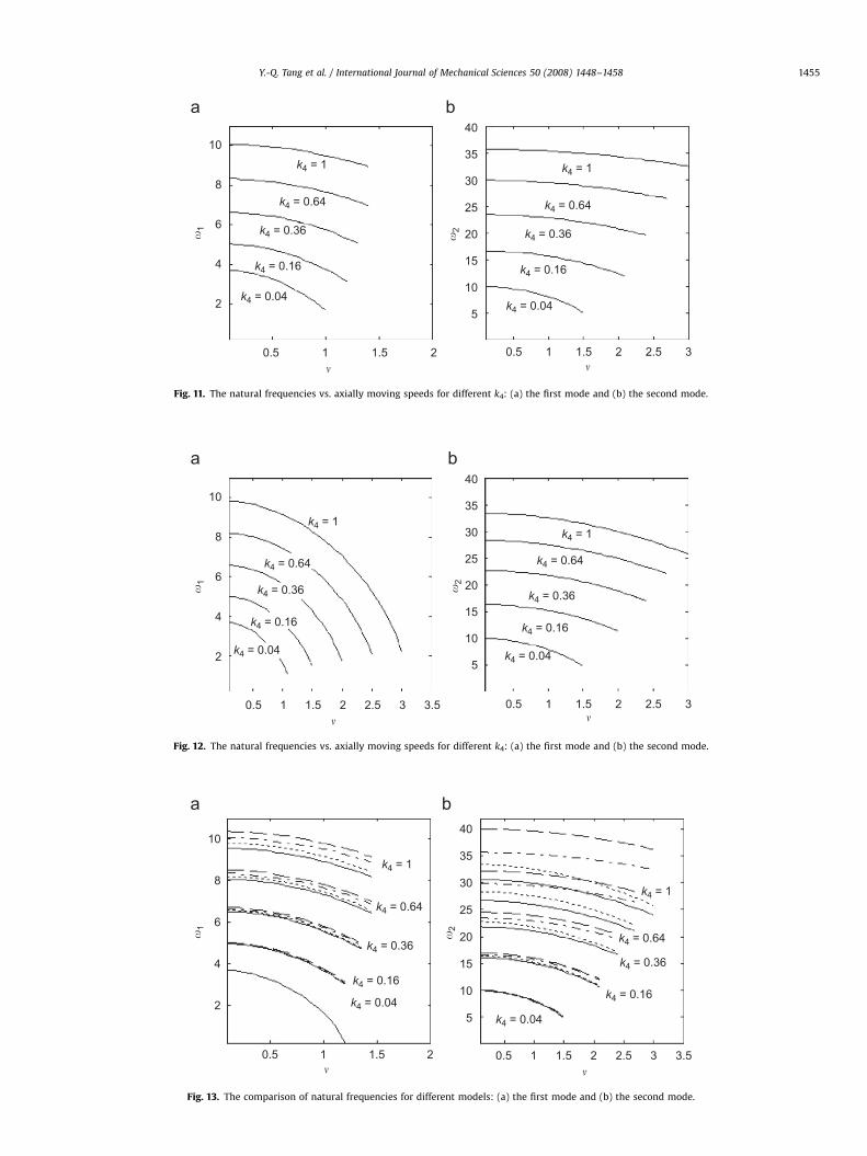
Fig. 12 presents the natural frequencies for the first and secondmodes, respectively.
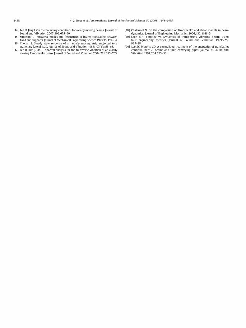
Fig. 13 presents the natural frequencies of the four models forthe first and second modes, respectively. The solid lines denote

ARTICLE IN PRESS
20
18
16
14
12
10
8
6
4
2
�1
�2
� �
k = 0
k = 2k = 6
k = 20
k = inf
k = 0k = 2
k = 6
k = 20
k = inf
45
40
35
30
25
20
150.5 1 1.5 2 2.5 31 2 3 4 5
Fig. 5. The natural frequencies vs. axially moving speeds for different spring stiffness: (a) the first mode and (b) the second mode.
1.5
1
0.5
0
-0.5
-1
-1.5
-2
-2.50 0.2 0.4 0.6 0.8 1
x x
�1
�2
Re
Re
Im
Im
3
2
1
0
-1
-2
-30 0.2 0.4 0.6 0.8 1
Fig. 6. The modal functions diagrams: (a) the first mode and (b) the second mode.
2
1
0
-1
-2
-30 0.2 0.4 0.6 0.8 1
x x
�1
�2
Re
Im
Re
Im
3
2
1
0
-1
-2
-30 0.2 0.4 0.6 0.8 1
Fig. 7. The contribution of axially moving speed to modal functions: (a) the first mode and (b) the second mode.
Y.-Q. Tang et al. / International Journal of Mechanical Sciences 50 (2008) 1448–1458 1453

ARTICLE IN PRESS
3
2
1
0
-1
-2
-30 0.2 0.4 0.6 0.8 1
x x
�1
�2
Re
Im
Re
Im
3
2
1
0
-1
-2
-30 0.2 0.4 0.6 0.8 1
Fig. 8. The contribution of spring stiffness to modal functions: (a) the first mode and (b) the second mode.
1.5
1
0.5
0
-0.5
-1
-1.5
-2
-2.5
-30 0.2 0.4 0.6 0.8 1
x x
�1
�2
3
2
1
0
-1
-2
-30 0.2 0.4 0.6 0.8 1
Im
Im
Re
Re
Fig. 9. The contribution of shear modulus to modal functions: (a) the first mode and (b) the second mode.
10
8
6
4
2
0.5 1 1.5� �
�1
�2
k4 = 1
k4 = 0.64
k4 = 0.36
k4 = 0.04
k4 = 0.16
k4 = 1
k4 = 0.64
k4 = 0.36
k4 = 0.04
k4 = 0.16
40
35
30
25
20
15
10
5
1 2 3 4 5 6
Fig. 10. The natural frequencies vs. axially moving speeds for different k4: (a) the first mode and (b) the second mode.
Y.-Q. Tang et al. / International Journal of Mechanical Sciences 50 (2008) 1448–14581454
ARTICLE IN PRESS
10
8
6
4
2
0.5 1 1.5 2� �
�1
�2
k4 = 1
k4 = 0.64
k4 = 0.36
k4 = 0.16
k4 = 0.04
k4 = 1
k4 = 0.64
k4 = 0.36
k4 = 0.16
k4 = 0.04
40
35
30
25
20
15
10
5
0.5 1 1.5 2 2.5 3
Fig. 11. The natural frequencies vs. axially moving speeds for different k4: (a) the first mode and (b) the second mode.
10
8
6
4
2
0.5 1 1.5 2 2.5 3 3.5�
�1
�2
k4 = 1
k4 = 0.64
k4 = 0.36
k4 = 0.16
k4 = 0.04
k4 = 1
k4 = 0.64
k4 = 0.36
k4 = 0.16
k4 = 0.04
40
35
30
25
20
15
10
5
0.5 1 1.5 2 2.5 3�
Fig. 12. The natural frequencies vs. axially moving speeds for different k4: (a) the first mode and (b) the second mode.
10
8
6
4
2
0.5 1 1.5 2�
�1
�2
40
35
30
25
20
15
10
5
0.5 1 1.5 2 2.5 3 3.5�
k4 = 1
k4 = 0.64
k4 = 0.36
k4 = 0.04
k4 = 0.16
k4 = 1
k4 = 0.64
k4 = 0.36
k4 = 0.04
k4 = 0.16
Fig. 13. The comparison of natural frequencies for different models: (a) the first mode and (b) the second mode.
Y.-Q. Tang et al. / International Journal of Mechanical Sciences 50 (2008) 1448–1458 1455

ARTICLE IN PRESS
4.6
4.4
Y.-Q. Tang et al. / International Journal of Mechanical Sciences 50 (2008) 1448–14581456
the Timoshenko model, the dotted lines denote the Shear model,the dash–dot lines denote the Rayleigh model and the dashedlines denote the Euler model.
4.2
4
3.8
3.6
3.4
3.2
3
2.8
2.60 20 40 60 80 100 120 140 160 180 200
k
�
Fig. 14. The critical speeds vs. spring stiffness.
2.8
2.6
2.4
2.2
2
1.8
1.6
1.4
1.20 0.1 0.2 0.3 0.4 0.5 0.6 0.7 0.8 0.9 1
k1
�
Fig. 15. The critical speeds vs. parameter k1.
5. The critical speeds
If Eq. (9) has a balanced solution, the time-independentequilibrium balance of the linear equation is
ðv2 � 1Þy;xx þ ðk1 þ k4 � k1v2Þy;xxxx ¼ 0 (35)
The boundary condition of simple supports with torsion springsdemands
yð0; tÞ ¼ yð1; tÞ ¼ 0; y;xxð0; tÞ � ky;x ¼ y;xxð1; tÞ þ ky;xð1; tÞ ¼ 0 (36)
The characteristic equation of Eq. (35) is
ðv2 � 1Þr2 þ ðk1 þ k4 � k1v2Þr4 ¼ 0 (37)
The solution of Eq. (37) is
r1 ¼ r2 ¼ 0; r3 ¼ r4 ¼ �i
ffiffiffiffiffiffiffiffiffiffiffiffiffiffiffiffiffiffiffiffiffiffiffiffiffiffiffiffiffiffiffiv2 � 1
k1 þ k4 � k1v2
s(38)
Then, the solution of Eq. (35) is
y ¼ C1 þ C2xþ C3 cos bxþ C4 sin bx (39)
where
b ¼
ffiffiffiffiffiffiffiffiffiffiffiffiffiffiffiffiffiffiffiffiffiffiffiffiffiffiffiffiffiffiffiv2 � 1
k1 þ k4 � k1v2
s(40)
Substituting Eq. (39) into (36) yields
1 0 1 0
0 �k �b2�kb
1 1 cos ðbÞ sin ðbÞ
0 k �b2 cos ðbÞ � kb sin ðbÞ kb cos ðbÞ � b2 sin ðbÞ
0BBBBB@
1CCCCCA
�
1
C2n
C3n
C4n
0BBBBB@
1CCCCCAC1n ¼ 0 (41)
For the non-trivial solution of Eq. (41), the determinant of thecoefficient matrix must be zero:
�2k2þ 2kðkþ b2
Þ cos ðbÞ � bð2k� k2þ b2Þ sin ðbÞ ¼ 0 (42)
Using Eqs. (40) and (42), one can obtain the critical speeds ofthe simple supports with torsion springs as follows:
v ¼
ffiffiffiffiffiffiffiffiffiffiffiffiffiffiffiffiffiffiffiffiffiffiffiffiffiffiffiffiffiffiffiffiffiðk1 þ k4Þb
2þ 1
1þ k1b2
vuut (43)
Fig. 14 presents the critical speeds of the simple supports withtorsion springs.
Substituting the spring stiffness k ¼ 0 into Eq. (42) yields
b ¼ np (44)
Then, one may get the critical velocity of the simple supports
v ¼
ffiffiffiffiffiffiffiffiffiffiffiffiffiffiffiffiffiffiffiffiffiffiffiffiffiffiffiffiffiffiffiffiffiffiffiffiffiffiðk1 þ k4Þn2p2 þ 1
1þ k1n2p2
snð1;¼ 2; 3; 4 . . .Þ (45)
Fig. 15 presents the critical speeds of the simple supports withparameter k1.
Substituting the spring stiffness k-N into Eq. (42) yields
b ¼ 2np (46)
Then, one may get the critical velocity of the fixed supports
v ¼
ffiffiffiffiffiffiffiffiffiffiffiffiffiffiffiffiffiffiffiffiffiffiffiffiffiffiffiffiffiffiffiffiffiffiffiffiffiffiffiffiffi4ðk1 þ k4Þn2p2 þ 1
1þ 4k1n2p2
snð1;¼ 2;3;4 . . .Þ (47)

ARTICLE IN PRESS
4.6
4
3.5
3
2.5
2
1.5
10 0.1 0.2 0.3 0.4 0.5 0.6 0.7 0.8 0.9 1
k1
�
Fig. 16. The critical speeds vs. parameter k1.
Y.-Q. Tang et al. / International Journal of Mechanical Sciences 50 (2008) 1448–1458 1457
Fig. 16 presents the critical speeds of the fixed supports withparameter k1.
6. Conclusions
In this investigation, natural frequencies, modes and criticalspeeds of axially moving beams on different supports areinvestigated based on the Timoshenko beam model. A differentiallinear equation of motion is derived from Newton’s second law.The frequencies and modes are investigated with the complexmode approach. At last, the expressions of the critical speeds forvarious boundary conditions are determined. Some numericalexamples are conducted to investigate the following:
The natural frequencies decrease with the increasing theaxially moving speed for simple supports and fixed supports.The symmetries decrease with the increase in spring stiffness forsimple supports with torsion springs.
For the efforts to modal functions, they have been found thatthe symmetries decrease with the increasing the spring stiffness,with the increasing the axial transport speeds and with thedecreasing the shear modulus.
The exact values at which the first natural frequency vanishesare called the critical speeds and afterwards the system isunstable. They can easily be got from the expressions. The criticalspeeds of the simple supports with torsion springs increase withthe increase in torsion spring stiffness. The critical speeds of thesimple supports and the fixed supports decrease with theincreasing the parameter k1.
Acknowledgements
This work was supported by the National Outstanding YoungScientists Fund of China (Project no. 10725209), the NationalNatural Science Foundation of China (Project no. 10672092), theShanghai Municipal Education Commission Scientific Research
Project (No. 07ZZ07), the Innovation Foundation for Graduates ofShanghai University (Project no. A.16-0401-08-005), and theShanghai Leading Academic Discipline Project (No. Y0103).
Appendix A
For the beam with the small deflection, the angle of the beam yis small. Thus,
cos y ¼ 1; y ¼ sin y ¼ Y ;X (A.1)
Substituting Eqs. (A.1) into (3) yields
�Q ;X � rAðY ;TT þ 2GY ;XT þ G2Y ;XXÞ þ PY ;XX ¼ 0 (A.2)
Substituting Eqs. (2) into (A.2) yields
c;X ¼ Y ;XX �krGðY ;TT þ 2GY ;XT þG2Y ;XXÞ þ
kP
AGY ;XX (A.3)
At both the ends, the beam has no transverse vibration. That isY ¼ 0. Thus Y,T ¼ 0, and further Y,TT ¼ 0 and Y,XT ¼ 0. At theboundaries, bending moment M is given by Eqs. (2) and (A.3) as
Because Eq. (A.3) is correct at arbitrary time,
MjX¼0;L ¼ EJ 1�krG
G2�kP
AG
� �Y ;XX jX¼0;L (A.4)
Substituting Eqs. (A.1) and (A.4) into (5)–(7) yields
YjX¼0 ¼ 0; YjX¼L ¼ 0; Y ;XX jX¼0 ¼ 0; Y ;XX jX¼L ¼ 0 (A.5)
YjX¼0 ¼ 0;YjX¼L ¼ 0; Y ;X jX¼0 ¼ 0;Y ;X jX¼L ¼ 0 (A.6)
YjX¼0 ¼ 0;YjX¼L ¼ 0; Y ;XX jX¼0 � mY ;X jX¼0 ¼ Y ;XX jX¼L þ mY ;X jX¼L ¼ 0
(A.7)
where
m ¼ K
EJð1� ðkr=GÞG2� ðkP=AGÞÞ
(A.8)
Eqs. (A.5)–(A.7) can easily lead to the dimensionless formEqs. (10)–(12).
References
[1] Mote Jr. CD. Dynamic stability of an axially moving band. Journal of theFranklin Institute 1968;285:329–46.
[2] Wickert JA, Mote Jr. CD. Classical vibration analysis of axially movingcontinua. ASME Journal of Applied Mechanics 1990;57:738–44.
[3] Oz HR, Pakdemirli M. Vibrations of an axially moving beam with timedependent velocity. Journal of Sound and Vibration 1999;227:239–57.
[4] Pakdemirli M, Oz HR. Infinite mode analysis and truncation to resonantmodes of axially accelerated beam vibrations. Journal of Sound and Vibration2008;311:1052–74.
[5] Oz HR. On the vibrations of an axially traveling beam on fixed supports withvariable velocity. Journal of Sound and Vibration 2001;239:556–64.
[6] Pakdemirli M, Ulsoy AG. Stability analysis of an axially accelerating string.Journal of Sound and Vibration 1997;203(5):815–32.
[7] Ozkaya E, Pakdemirli M. Vibrations of an axially accelerating beam with smallflexural stiffness. Journal of Sound and Vibration 2000;234:521–35.
[8] Ozkaya E, Oz HR. Determination of natural frequencies and stability regions ofaxially moving beams using artificial neural networks method. Journal ofSound and Vibration 2002;254:782–9.
[9] Oz HR. Natural frequencies of axially travelling tensioned beams in contactwith a stationary mass. Journal of Sound and Vibration 2003;259:445–56.
[10] Kong L, Parker RG. Approximate eigensolutions of axially moving beams withsmall flexural stiffness. Journal of Sound and Vibration 2004;276:459–69.
[11] Ghayesh MH, Khadem SE. Rotary inertia and temperature effects on non-linear vibration, steady-state response and stability of an axially movingbeam with time-dependent velocity. International Journal of MechanicalSciences 2008;50:389–404.
[12] Yang XD, Chen LQ. The stability of an axially acceleration beam on simplesupports with torsion springs. Acta Mechanica Solida Sinica 2005;18:1–8.
[13] Chen LQ, Yang XD. Vibration and stability of an axially moving viscoelasticbeam with hybrid supports. European Journal of Mechanics A/Solids 2006;25:996–1008.
ARTICLE IN PRESS
Y.-Q. Tang et al. / International Journal of Mechanical Sciences 50 (2008) 1448–14581458
[14] Lee U, Jang I. On the boundary conditions for axially moving beams. Journal ofSound and Vibration 2007;306:675–90.
[15] Simpson A. Transverse modes and frequencies of beams translating betweenfixed end supports. Journal of Mechanical Engineering Science 1973;15:159–64.
[16] Chonan S. Steady state response of an axially moving strip subjected to astationary lateral load. Journal of Sound and Vibration 1986;107(1):155–65.
[17] Lee U, Kim J, Oh H. Spectral analysis for the transverse vibration of an axiallymoving Timoshenko beam. Journal of Sound and Vibration 2004;271:685–703.
[18] Challamel N. On the comparison of Timoshenko and shear models in beamdynamics. Journal of Engineering Mechanics 2006;132:1141–5.
[19] Seon MH, Timothy W. Dynamics of transversely vibrating beams usingfour engineering theories. Journal of Sound and Vibration 1999;225:935–88.
[20] Lee SY, Mote Jr. CD. A generalized treatment of the energetics of translatingcontinua, part 2: beams and fluid conveying pipes. Journal of Sound andVibration 1997;204:735–53.
Related Documents