National Oceanography Centre Cruise Report No. 27 RRS ...

National Oceanography Centre

Cruise Report No. 27

RRS James Cook Cruise 87 31 MAY - 18 JUN 2013

The Twilight Cruise to the Porcupine Abyssal Plain

Sustained Observatory

Principal Scientist R S Lampitt

2015

National Oceanography Centre, Southampton University of Southampton Waterfront Campus European Way Southampton Hants SO14 3ZH UK Tel: +44 (0)23 8059 6347 Email: [email protected]

© National Oceanography Centre, 2015

DOCUMENT DATA SHEET

AUTHOR

LAMPITT, R S et al PUBLICATION DATE 2015

TITLE RRS James Cook Cruise 87, 31 May - 18 Jun 2013. The Twilight Cruise to the Porcupine Abyssal Plain Sustained Observatory.

REFERENCE Southampton, UK: National Oceanography Centre, Southampton, 114pp.

(National Oceanography Centre Cruise Report, No. 27) ABSTRACT

The Twilight Zone is that depth zone in the ocean between 100 and 1000m depth where a

tremendous amount of activity takes place. Much of the material containing carbon which

sinks out of the upper sunlit or "Euphotic" zone is broken down in the twilight zone and then

mixes back up to the surface in the winter. If it manages to sink further, this carbon is lost for

periods of centuries.

The main factor that affects this sedimentation process and the rate of destruction of the sinking

particles is the structure and function of the biological community living near the sea surface

and in the twilight zone beneath. This is because the planktonic plants and animals living there

both generate and destroy particles. The Porcupine Abyssal Plain sustained observatory (PAP)

is a heavily instrumented area of the open ocean 350 miles southwest of Ireland and in a water

depth of 4800m. The instruments measure a wide variety of properties of the environment

above the water, within it and on the seabed and much of the data is transmitted in real time to

land via satellite.

    KEYWORDS

ISSUING ORGANISATION National Oceanography Centre University of Southampton Waterfront Campus European Way Southampton SO14 3ZH UK Tel: +44(0)23 80596116 Email: [email protected]

A pdf of this report is available for download at: http://eprints.soton.ac.uk

Page intentionally left blank

5

Contents 1 Scientific Personnel ..................................................................................................................... 7

2 Ships Personnel ............................................................................................................................ 7

3 Itinerary ........................................................................................................................................ 9

4 Background & Objectives .......................................................................................................... 11

5 Activity Reports ......................................................................................................................... 12

5.1 Ocean Acidification Experiment ......................................................................................... 12 5.2 Atmospheric Deposition ...................................................................................................... 14 5.3 N Cycle Measurements ....................................................................................................... 15 5.4 Small Zooplankton .............................................................................................................. 19 5.5 Community Oxygen Dynamics (Consumption/Production) ............................................... 22 5.6 Blog “Down to the Twilight Zone” ..................................................................................... 26 5.7 Particle Flux through the Twilight Zone ............................................................................. 29 5.8 Molecular Variation of Lipids in Particles .......................................................................... 36 5.9 Video Plankton Recorder .................................................................................................... 40 5.10 Marine Snow Analysis ........................................................................................................ 45 5.11 Pelagra ................................................................................................................................. 50

5.11.1 Camera Test ................................................................................................................. 51 5.11.2 Deployment 1 (Ballast Tests)....................................................................................... 52 5.11.3 Deployment 2 ............................................................................................................... 55 5.11.4 Deployment 3 ............................................................................................................... 60

5.12 Camera Profiles ................................................................................................................... 64 5.13 Mesozooplankton Studies ................................................................................................... 65 5.14 Underway Sampling ............................................................................................................ 68 5.15 13C-based Primary Production and other parameters ......................................................... 70 5.16 Turbulence Measurements .................................................................................................. 74 5.17 Dissolved Oxygen Analysis ................................................................................................ 80 5.18 Cytometry Sampling ........................................................................................................... 83 5.19 Nutrient Analysis................................................................................................................. 85 5.20 Chlorophyll-a Measurement ................................................................................................ 89 5.21 Sea Mammal Sound Records .............................................................................................. 90 5.22 OSMOSIS Seaglider Turnaround ....................................................................................... 94

6 Station List ............................................................................................................................... 100

7 Appendix I Station List JC087 CTD Salinity bottle logsheet .................................................. 108

8 Appendix II Station List JC087 PP samples ............................................................................ 114

6

7

1 Scientific Personnel

Family Name Given Names Rank or Rating 1 LAMPITT RICHARD STEPHEN PSO 2 MARTIN ADRIAN PETER Scientist 3 STINCHCOMBE MARK COLIN Technician 4 SAW KEVIN ANTONY Engineer 5 BELCHER ANNA Scientist 6 BIRCHILL ANTHONY JAMES Student 7 WILLMOT OLIVER ROGER Student 8 MORRALL ZOE ELIZABETH Student 9 RUMYANTSEVA ANNA CHRISTINE Student 10 DUDEJA GAYATRI Student 11 DAVEY EMILY Student 12 YUMRUKTEPE CAGLAR VELI Student 13 IBELLO VALERIA Scientist 14 KOSKI MARJA KAARINA Scientist 15 VALENCIA-RAMIREZ BELLINETH Scientist 16 LINDEMANN CHRISTIAN Scientist 17 IVERSEN MORTEN Scientist 18 GASPAROVIC BLAZENKA Scientist 19 NORRBIN FREDRIKA Scientist 20 WILSON STEPHANIE Scientist 21 THIELE CHRISTINA Student 22 NEWSTEAD REBEKAH Student 23 DAMERELL GILLIAN Student

2 Ships Personnel Family Name Given Names Rank or Rating

1 LEASK JOHN ALAN Master 2 WARNER RICHARD ALAN C/O 3 GRAVES MALCOLM HAROLD 2/O 4 NORRISH NICHOLAS 3/O 5 PARKINSON GEORGE GRANT C/E 6 MURRAY MICHAEL 2/E 7 MURREN MICHAEL GERARD 3/E 8 DAVITT FRANCIS ROBERT 3/E 9 ULBRICHT SEBASTIAN MARTIN ETO

10 ROGERS MARK ALAN ETO 11 McDOUGALL PAULA ANNE PCO 12 HARRISON MARTIN ANDREW CPOS 13 ALLISON PHILIP CPOD 14 SMITH PETER CPO 15 HOPLEY JOHN SG1A 16 MOORE MARK STEPHEN SG1a 17 TONER STEPHEN SG1A 18 WELTON JARROD DAVID SG1A 19 CONTEH BRIAN ERPO 20 LYNCH PETER ANTHONY H/Chef 21 SUTTON LLOYD SPENCER Chef 22 ROBINSON PETER WAYNE Stwd 23 PIPER CARL A/Stwd

8

9

3 Itinerary

RRS James Cook slipped her moorings in the Port of Glasgow at 0815h BST on 31st May 2013. A request to rescue a flooded glider to the north of Ireland meant a detour was carried out on passage to PAP but this successful recovery did set the tone for the rest of the cruise. Downtime due to bad weather or faults of shipboard or overside equipment was minimal and did not affect the outcome of the cruise in any major way.

A location was selected within the OSMOSIS mooring array at PAP for the most intensive sampling in order to provide a very much better physical context than is usually possible. This was certainly the best ever achieved at PAP and possibly anywhere for a cruise which had the primary focus of biology and biogeochemistry. This location, termed “The Twilight Station” was more than 4km from any of the OSMOSIS moorings to ensure there was no entanglement with them.

A feature of the site was that in contrast to previous years, there was a strong and persistent westerly current over the top few hundred meters of the water column. The effect of this was that the PELAGRA drifting sediment traps which were intended to provide a direct measure of downward particle flux at the twilight station rapidly exited the region after every deployment.

Most aspects of the sampling and experimentation during JC087 were highly successful although almost continuous cloud cover removed the possibility of satellite remote sensing data which was to provide the spatial context for our work.

RRS James Cook left PAP at 1645h GMT on 14th June 2013, 13 hours earlier than planned due to the possibility of poor weather on the return passage. The ship reached the Port of Glasgow in the early evening of 17th June, the day before that expected.

10

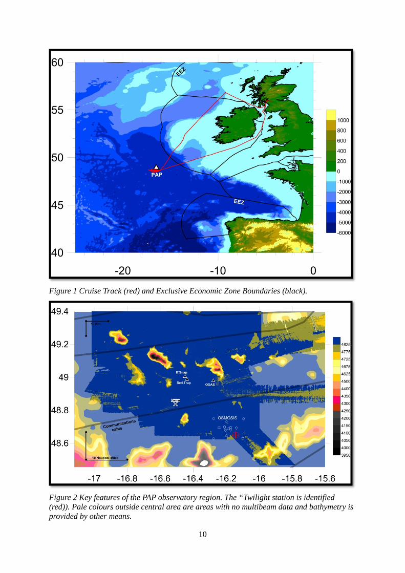
Figure 1 Cruise Track (red) and Exclusive Economic Zone Boundaries (black).

Figure 2 Key features of the PAP observatory region. The “Twilight station is identified (red)). Pale colours outside central area are areas with no multibeam data and bathymetry is provided by other means.

11

4 Background & Objectives The twilight zone is that depth zone in the ocean between 100 and 1000m depth where a tremendous amount of activity takes place. Much of the material containing carbon which sinks out of the upper sunlit or “Euphotic” zone is broken down in the twilight zone and then mixes back up to the surface in the winter. If it manages to sink further, this carbon is lost for periods of centuries. The main factor that affects this sedimentation process and the rate of destruction of the sinking particles is the structure and function of the biological community living near the sea surface and in the twilight zone beneath. This is because the planktonic plants and animals living there both generate and destroy particles. The Porcupine Abyssal Plain sustained observatory (PAP) is a heavily instrumented area of the open ocean 350 miles southwest of Ireland and in a water depth of 4800m. The instruments measure a wide variety of properties of the environment above the water, within it and on the seabed and much of the data is transmitted in real time to land via satellite. http://www.eurosites.info/pap/data.php Although most of these data concern the biology and chemistry of the water column and seabed, for this particular year there is also a major physical oceanography programme at the site. This programme called OSMOSIS aims to examine the processes of mixing in the upper Ocean and employs an array of moorings and two permanent gliders which cruise around them undulating over the top 1000m. This cruise involves 19 research scientists from 7 European nations bringing together a very wide range of expertise including chemists, biologists, physicists and biogeochemical modellers. Many of these individuals are involved with the EU programme EuroBASIN. EuroBASIN is part of the trans-Atlantic BASIN initiative. This involves scientists from US, Canada and EU who are investigating how climatic and human activity affects the North Atlantic ecosystem. The objective of the cruise is to use a wide variety of approaches to characterise the biological communities in the Euphotic and Twilight zones using water bottles, nets and video systems. We then characterise the chemical and physical environment and examine the sinking particles and the rate of downward flux of material using water samples, photographic approaches and the free drifting sediment trap PELAGRA.

12

5 Activity Reports

5.1 Ocean Acidification Experiment Valeria Ibello Objective The aim of the ocean acidification experiment is to evaluate the effect of decrease of pH on nitrifying bacteria in the ocean upper layer. It has been observed that decrease of pH can strongly inhibit nitrifying bacteria, because in lower pH conditions, the NH3/NH4+ ratio tends to decrease and the substrate for nitrifying bacteria (NH3) disappears (Huesemann et al. 2002, Beman et al. 2011). The ultimate objective, therefore, is to understand how changes of nitrate production can impact on primary production during the summer season where stratification limits the uplifting of deep nitrate and the only nitrate available is produced by nitrification processes. Method Ocean acidification experiment was carried on 14/06/2013 (ctd # 24). Seawater was collected from one single depth at 40 m corresponding to 1% of PAR, where highest nitrification rates were generally observed. Samples for dissolved inorganic carbon (DIC) and total alkalinity (TA) were immediately collected in 250 ml Duran Schott glass bottles, poisoned with 50µl of HgCl2 saturated solution, sealed and stored till analysis at home laboratory, accordingly with the procedure recommended by Dickson et al. (2007). Samples for acidification experiments were immediately added with 15N-NH4+ and incubated for 30 minutes to homogenize the sample. 3 samples were manipulated with opportune addition of HCl and NaHCO3 to reach approximately pCO2 450, 600 and 750 µatm. One sample was not pH altered to be used as control. All bottles were sealed avoiding any air bubble inside. After 24 h incubation at controlled light and temperature, DIC, TA and nitrification rates were sub-sampled. Samples for nitrification rates were stored in 100 ml HDPE Nalgene bottles and immediately frozen till analyses in home laboratory. All samples were collected in triplicates. During all operations, samples were in contact with the atmosphere for very limited time to avoid CO2 exchange. Nutrients were sub-samples at the beginning and at the end of the experiment. In addition, single samples for DIC and TA were collected from the deep cast along all water column (depths: 2, 5, 10, 15, 25, 35, 40, 65, 100, 150, 200, 400, 600, 800, 1000, 1500, 2000, 2250, 2500, 2750, 3000, 3250, 3500, 3750, 4000, 4500, 4800 m).

13

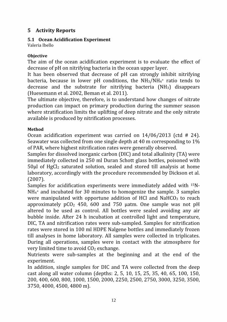
Nitrification Rates Nitrification rates will be determined with the tracer addition method. Briefly, samples were added with about 10% of NH4+ ambient concentration nM of 99 atom percent (at%) stable isotope tracer (15NH4+). Nitrification rates will be calculated by measuring the accumulation of 15N label in the oxidized NO2 + NO3- pool following incubation for 24h. The method that will be used to determine 15N produced by nitrification is the so called 'denitrifier method' using denitryfying bacteria to convert NO2- and NO3- in N2O (Sigman et al. 2001). Carbonate System Seawater CO2 parameters will be determined by measurement of two carbonate system parameters: total TA and DIC concentration. pH will be calculated. DIC and TA measurements will be undertaken using a VINDTA 3C (Marianda, Germany) at NOC. DIC will be determined using a coulometric titration (coulometer 5011, UIC, USA) and TA will be determined using a closed-cell titration procedure (Dickson et al. 2007). Scheme of the ocean acidification experiment

Figure 3schematic of ocean acidification experiment

References Beman and Others, 2011. Global declines in oceanic nitrification rates as a consequence of ocean acidification. Proc. Natl. Acad. Sci. USA 108: 208–213,

doi:10.1073/pnas.1011053108 Dickson A. G., Sabine C. L. & Christian J. R. (Eds.), 2007. Guide to best practices for ocean

CO2 measurements. PICES Special Publication 3: 1-191. Huesemann MH, Skillman AD, Crecelius EA (2002) The inhibition of marine nitrification

by ocean disposal of carbon dioxide. Mar Pollut Bull 44:142–148. Sigman DM, et al. (2001) A bacterial method for the nitrogen isotopic analysis of nitrate

in seawater and freshwater. Anal Chem 73:4145–4153.

14

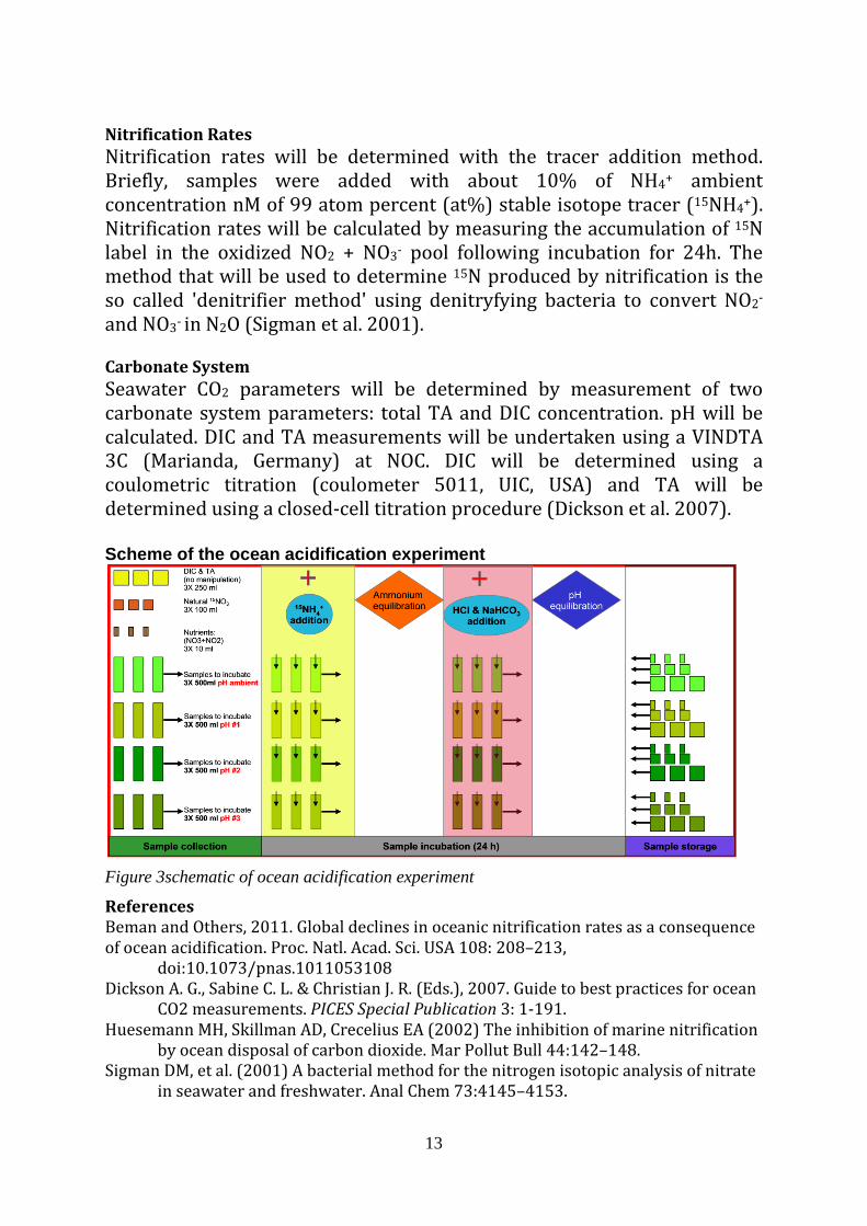
5.2 Atmospheric Deposition Anthony Birchill, Caglar V. Yumruktepe and Valeria Ibello Objective Aerosol samples was collected to i) estimate aerosol deposition rates at PAP, ii) evaluate the bioavailability of aerosol in surface seawater, and iii) explore the impact of the ocean acidification on the aerosol availability in surface seawater. The nutrient/metals investigated are - NO3-, NH4+, PO43-, Zn, Cu, Pb, Cd. Methods Atmospheric sampling was conducted on the RRS James Cook's monkey island, at more of 20 m distant from the chimney flue. In order to avoid contamination from the ship's stacks, the air sampling system incorporated an automatic switch connecting a wind vane to the air pump engine to activate/deactivate air sampling accordingly with wind direction. A total of 9 bulk aerosol filter samples were collected using a low volume air sampling system (flow rates approximately 10 l min−1) on a 0.2 µm polycarbonate filter (45 mm diameter), for typically 24 h. Due to an initial problem occurred at the air pump, the aerosol sampling started 3 days later the start of water measurements. Details of the sampling log are reported in Table 1 below.

Table 1 Summary of Atmospheric Samples Collected.

Sampling Day (mm-dd-yy) Air Volume Time (GMT) Weather Coordinates (LAT / LON) Jul Day

ATM01

From 06-06-13 20768247 21:00:00 partly cloudy 48.38.915N / 16.08.571W 157

To 06-07-13 20784512 20:00:00 Cloudy 48.38.917N / 16.08.571W 158

ATM02

From 06-07-13 20784512 20:32:00 partly cloudy 48.38.916N / 16.08.571W 158

To 06-08-13 20797970 19:40:00 partly cloudy 48.29.317N / 16.41.05W 159

ATM03

From 06-08-13 20803673 20:00:00 Clear 48.29.317N / 16.41.05W 159

To 06-09-13 20803899 09:51:00 Rainy 48.38.916N / 16.08.573W 160

ATM04

From 06-09-13 20803899 10:28:00 rainy 48.38.916N / 16.08.573W 160

To 06-10-13 20810920 10:00:00 overcast 48.38.549N / 16.08.344W 161

ATM05

From 06-10-13 20810920 10:25:00 overcast 48.38.550N / 16.08.344W 161

To 06-11-13 20820782 12:48:00 cloudy 48.46.382N / 16.39.943W 162

ATM06

From 06-11-13 20820782 13:09:00 cloudy 48.46.371N / 16.40.103W 162

To 06-12-13 20830328 18:53:00 storm 48.30.011N / 16.53.712W 163

ATM07

From 06-12-13 20830328 19:09:00 clear/windy 48.30.012N / 16.52.28W 163

To 06-13-13 20840694 18:23:00 cloudy/windy 48.38.918N / 16.08.5748W 164

ATM08

From 06-13-13 20840694 18:47:00 cloudy/windy 48.38.914N / 16.08.573W 164

To 06-14-13 20852248 19:57:00 clear/windy 48.52.719N / 15.23.569W 165

ATM09

From 06-14-13 20852268 20:19:00 clear/windy 48.52.743N / 15.08.617W 165

To 06-15-13 20853069 19:06:00 cloudy 50.35.812W / 09.48.421W 166

15

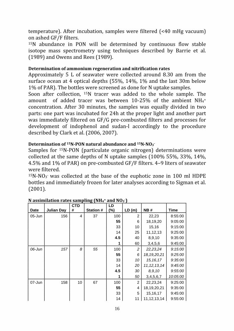
All subsequent analysis will take place at home laboratories. In the case of ammonia analyses it will be required to determine if the system has the sensitivity to measure ambient concentrations over blanks. Tests on nutrients bioavailability will be done on filtered surface seawater collected at PAP. pH manipulation and carbonate system analysis will follow the same procedure/methods of the ocean acidification experiment described in the N cycle measurements section. Analysis will be carried out using Ion Chromatography and Auto-analyzer. For experiments on nutrient bioavailability, sea-water will be purified by Chelex-100. 5.3 N Cycle Measurements Anthony Birchill, Oliver Wilmott, Caglar V. Yumruktepe and Valeria Ibello Objective The main objective of the JC87 cruise was to estimate new and regenerated primary production and nitrification rates Different processes of the N cycle will be tackled (ammonium and nitrate assimilation rates, ammonium regeneration and nitrification rates) in order to obtain estimates of f ratio. New primary production rates will be used to calculate C export from the euphotic zone. Furthermore, natural abundance of the stable 15N isotope in particulate organic nitrogen (PON) and in nitrate at the base of the euphotic zone will be determined to evaluate the origin of N sources (N deposition, N2 fixation, deep nitrate) used by phytoplankton. Methods Determination of ammonium and nitrate assimilation rates Seawater was collected around 8.30 a.m. for 9 days from the surface ocean at 6 optical depths: 100% 55%, 33%, 14%, 4.5% and 1% of surface radiation. PAR profile was determined from the same CTD during the down cast deployment. Samples were collected in triplicates in 670 ml acid washed, 3 times milliQ rinsed, polycarbonate clear bottles screened with combination of neutral and blue light filters. Assimilation rates for NO3- and NH4+ will be determined following the incorporation of the stable isotope 15N-NH4+ and 15N-NO3- in PON. Ideally, addition of enriched daily-prepared standard was within 10% of nutrient ambient concentration, calculated on the base of nutrients vertical profile of the day before. In oligotrophic conditions, the minimum addition was 5 nmol/l. After 15N-NH4+ and 15N-NO3- addition, samples were incubated for 4-6 hours. Incubations were made in an on-deck incubator cooled with at surface seawater (temperature was maximum 2° C warmer than the in situ

16

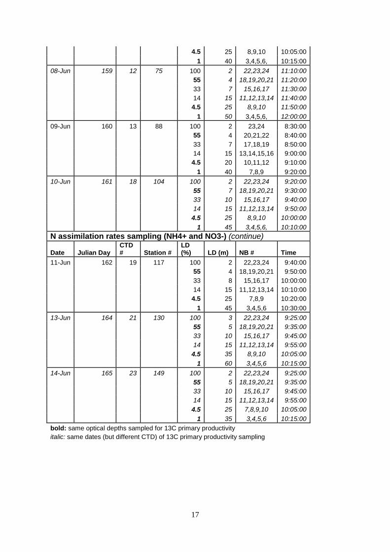
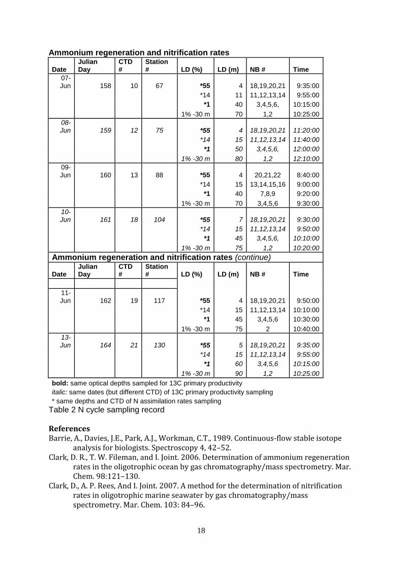
temperature). After incubation, samples were filtered (<40 mHg vacuum) on ashed GF/F filters. 15N abundance in PON will be determined by continuous flow stable isotope mass spectrometry using techniques described by Barrie et al. (1989) and Owens and Rees (1989). Determination of ammonium regeneration and nitrification rates Approximately 5 L of seawater were collected around 8.30 am from the surface ocean at 4 optical depths (55%, 14%, 1% and the last 30m below 1% of PAR). The bottles were screened as done for N uptake samples. Soon after collection, 15N tracer was added to the whole sample. The amount of added tracer was between 10-25% of the ambient NH4+ concentration. After 30 minutes, the samples was equally divided in two parts: one part was incubated for 24h at the proper light and another part was immediately filtered on GF/G pre-combusted filters and processes for development of indophenol and sudan-l accordingly to the procedure described by Clark et al. (2006, 2007). Determination of 15N-PON natural abundance and 15N-NO3- Samples for 15N-PON (particulate organic nitrogen) determinations were collected at the same depths of N uptake samples (100% 55%, 33%, 14%, 4.5% and 1% of PAR) on pre-combusted GF/F filters. 4–9 liters of seawater were filtered. 15N-NO3- was collected at the base of the euphotic zone in 100 ml HDPE bottles and immediately frozen for later analyses according to Sigman et al. (2001). N assimilation rates sampling (NH4+ and NO3-)

Date Julian Day CTD # Station #

LD (%) LD (m) NB # Time

05-Jun 156 4 37 100 2 22,23 8:55:00 55 6 18,19,20 9:05:00 33 10 15,16 9:15:00 14 25 11,12,13 9:25:00 4.5 40 8,9,10 9:35:00 1 60 3,4,5,6 9:45:00 06-Jun 157 8 55 100 2 22,23,24 9:15:00 55 6 18,19,20,21 9:25:00 33 10 15,16,17 9:35:00 14 20 11,12,13,14 9:45:00 4.5 30 8,9,10 9:55:00 1 50 3,4,5,6,7 10:05:00 07-Jun 158 10 67 100 2 22,23,24 9:25:00 55 4 18,19,20,21 9:35:00 33 5 15,16,17 9:45:00 14 11 11,12,13,14 9:55:00

17

4.5 25 8,9,10 10:05:00 1 40 3,4,5,6, 10:15:00 08-Jun 159 12 75 100 2 22,23,24 11:10:00 55 4 18,19,20,21 11:20:00 33 7 15,16,17 11:30:00 14 15 11,12,13,14 11:40:00 4.5 25 8,9,10 11:50:00 1 50 3,4,5,6, 12:00:00 09-Jun 160 13 88 100 2 23,24 8:30:00 55 4 20,21,22 8:40:00 33 7 17,18,19 8:50:00 14 15 13,14,15,16 9:00:00 4.5 20 10,11,12 9:10:00 1 40 7,8,9 9:20:00 10-Jun 161 18 104 100 2 22,23,24 9:20:00 55 7 18,19,20,21 9:30:00 33 10 15,16,17 9:40:00 14 15 11,12,13,14 9:50:00 4.5 25 8,9,10 10:00:00 1 45 3,4,5,6, 10:10:00 N assimilation rates sampling (NH4+ and NO3-) (continue)

Date Julian Day CTD # Station #

LD (%) LD (m) NB # Time

11-Jun 162 19 117 100 2 22,23,24 9:40:00 55 4 18,19,20,21 9:50:00 33 8 15,16,17 10:00:00 14 15 11,12,13,14 10:10:00 4.5 25 7,8,9 10:20:00 1 45 3,4,5,6 10:30:00 13-Jun 164 21 130 100 3 22,23,24 9:25:00 55 5 18,19,20,21 9:35:00 33 10 15,16,17 9:45:00 14 15 11,12,13,14 9:55:00 4.5 35 8,9,10 10:05:00 1 60 3,4,5,6 10:15:00 14-Jun 165 23 149 100 2 22,23,24 9:25:00 55 5 18,19,20,21 9:35:00 33 10 15,16,17 9:45:00 14 15 11,12,13,14 9:55:00 4.5 25 7,8,9,10 10:05:00 1 35 3,4,5,6 10:15:00 bold: same optical depths sampled for 13C primary productivity italic: same dates (but different CTD) of 13C primary productivity sampling

18

Ammonium regeneration and nitrification rates

Date Julian Day

CTD #

Station # LD (%) LD (m) NB # Time

07-Jun 158 10 67 *55 4 18,19,20,21 9:35:00

*14 11 11,12,13,14 9:55:00 *1 40 3,4,5,6, 10:15:00 1% -30 m 70 1,2 10:25:00

08-Jun 159 12 75 *55 4 18,19,20,21 11:20:00

*14 15 11,12,13,14 11:40:00 *1 50 3,4,5,6, 12:00:00 1% -30 m 80 1,2 12:10:00

09-Jun 160 13 88 *55 4 20,21,22 8:40:00

*14 15 13,14,15,16 9:00:00 *1 40 7,8,9 9:20:00 1% -30 m 70 3,4,5,6 9:30:00

10-Jun 161 18 104 *55 7 18,19,20,21 9:30:00

*14 15 11,12,13,14 9:50:00 *1 45 3,4,5,6, 10:10:00 1% -30 m 75 1,2 10:20:00 Ammonium regeneration and nitrification rates (continue)

Date Julian Day

CTD #

Station # LD (%) LD (m) NB # Time

11-Jun 162 19 117 *55 4 18,19,20,21 9:50:00

*14 15 11,12,13,14 10:10:00 *1 45 3,4,5,6 10:30:00 1% -30 m 75 2 10:40:00

13-Jun 164 21 130 *55 5 18,19,20,21 9:35:00

*14 15 11,12,13,14 9:55:00 *1 60 3,4,5,6 10:15:00 1% -30 m 90 1,2 10:25:00 bold: same optical depths sampled for 13C primary productivity italic: same dates (but different CTD) of 13C primary productivity sampling * same depths and CTD of N assimilation rates sampling

Table 2 N cycle sampling record References Barrie, A., Davies, J.E., Park, A.J., Workman, C.T., 1989. Continuous-flow stable isotope

analysis for biologists. Spectroscopy 4, 42–52. Clark, D. R., T. W. Fileman, and I. Joint. 2006. Determination of ammonium regeneration

rates in the oligotrophic ocean by gas chromatography/mass spectrometry. Mar. Chem. 98:121–130.

Clark, D., A. P. Rees, And I. Joint. 2007. A method for the determination of nitrification rates in oligotrophic marine seawater by gas chromatography/mass spectrometry. Mar. Chem. 103: 84–96.

19

Owens, N.J.P., Rees, A.P., 1989. Determination of nitrogen-15 at sub-microgram levels of nitrogen using automated continuous flow isotope ratio mass spectrometry. Analyst 114, 1655–1657.

Sigman DM, et al. (2001) A bacterial method for the nitrogen isotopic analysis of nitrate in seawater and freshwater. Anal Chem 73:4145–4153.

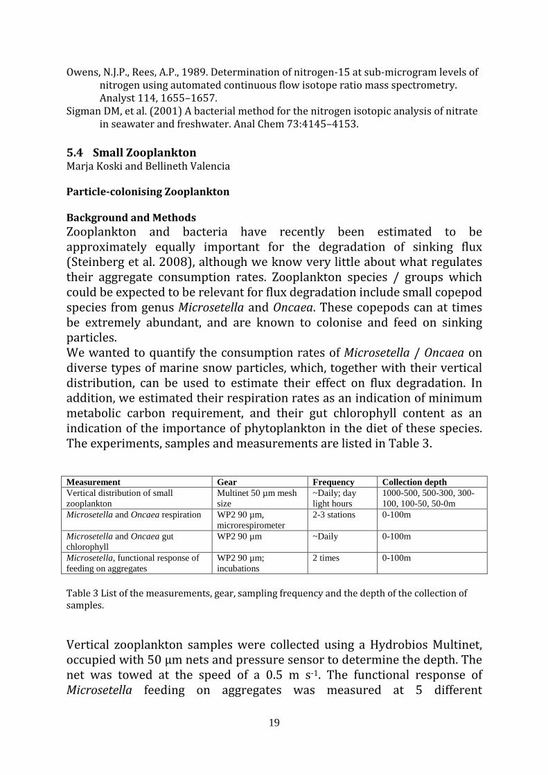
5.4 Small Zooplankton Marja Koski and Bellineth Valencia Particle-colonising Zooplankton Background and Methods Zooplankton and bacteria have recently been estimated to be approximately equally important for the degradation of sinking flux (Steinberg et al. 2008), although we know very little about what regulates their aggregate consumption rates. Zooplankton species / groups which could be expected to be relevant for flux degradation include small copepod species from genus Microsetella and Oncaea. These copepods can at times be extremely abundant, and are known to colonise and feed on sinking particles. We wanted to quantify the consumption rates of Microsetella / Oncaea on diverse types of marine snow particles, which, together with their vertical distribution, can be used to estimate their effect on flux degradation. In addition, we estimated their respiration rates as an indication of minimum metabolic carbon requirement, and their gut chlorophyll content as an indication of the importance of phytoplankton in the diet of these species. The experiments, samples and measurements are listed in Table 3. Measurement Gear Frequency Collection depth Vertical distribution of small zooplankton

Multinet 50 µm mesh size

~Daily; day light hours

1000-500, 500-300, 300-100, 100-50, 50-0m

Microsetella and Oncaea respiration WP2 90 µm, microrespirometer

2-3 stations 0-100m

Microsetella and Oncaea gut chlorophyll

WP2 90 µm ~Daily 0-100m

Microsetella, functional response of feeding on aggregates

WP2 90 µm; incubations

2 times 0-100m

Table 3 List of the measurements, gear, sampling frequency and the depth of the collection of samples. Vertical zooplankton samples were collected using a Hydrobios Multinet, occupied with 50 µm nets and pressure sensor to determine the depth. The net was towed at the speed of a 0.5 m s-1. The functional response of Microsetella feeding on aggregates was measured at 5 different

20

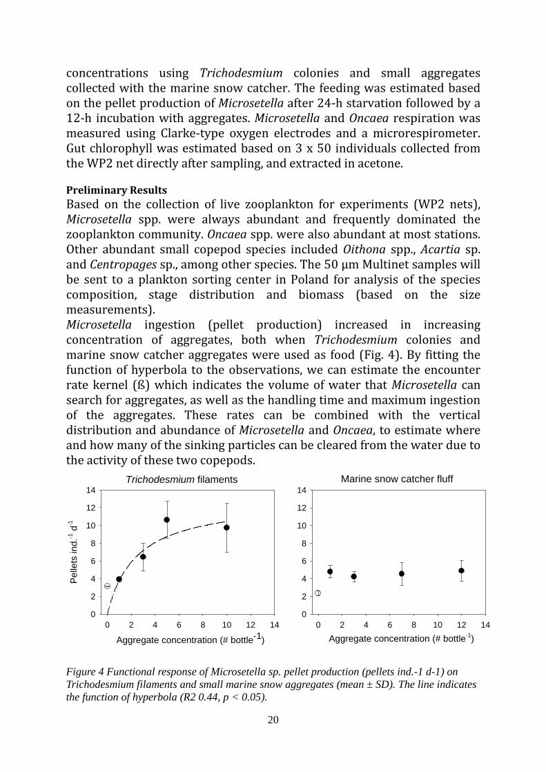
concentrations using Trichodesmium colonies and small aggregates collected with the marine snow catcher. The feeding was estimated based on the pellet production of Microsetella after 24-h starvation followed by a 12-h incubation with aggregates. Microsetella and Oncaea respiration was measured using Clarke-type oxygen electrodes and a microrespirometer. Gut chlorophyll was estimated based on 3 x 50 individuals collected from the WP2 net directly after sampling, and extracted in acetone. Preliminary Results Based on the collection of live zooplankton for experiments (WP2 nets), Microsetella spp. were always abundant and frequently dominated the zooplankton community. Oncaea spp. were also abundant at most stations. Other abundant small copepod species included Oithona spp., Acartia sp. and Centropages sp., among other species. The 50 µm Multinet samples will be sent to a plankton sorting center in Poland for analysis of the species composition, stage distribution and biomass (based on the size measurements). Microsetella ingestion (pellet production) increased in increasing concentration of aggregates, both when Trichodesmium colonies and marine snow catcher aggregates were used as food (Fig. 4). By fitting the function of hyperbola to the observations, we can estimate the encounter rate kernel (ß) which indicates the volume of water that Microsetella can search for aggregates, as well as the handling time and maximum ingestion of the aggregates. These rates can be combined with the vertical distribution and abundance of Microsetella and Oncaea, to estimate where and how many of the sinking particles can be cleared from the water due to the activity of these two copepods.

Trichodesmium filaments

Aggregate concentration (# bottle-1)

0 2 4 6 8 10 12 14

Pelle

ts in

d.-1

d-1

0

2

4

6

8

10

12

14Marine snow catcher fluff

Aggregate concentration (# bottle-1)0 2 4 6 8 10 12 14

0

2

4

6

8

10

12

14

Figure 4 Functional response of Microsetella sp. pellet production (pellets ind.-1 d-1) on Trichodesmium filaments and small marine snow aggregates (mean ± SD). The line indicates the function of hyperbola (R2 0.44, p < 0.05).

21

Centropages sp. as a representative of small calanoids Background and Methods Many calanoid copepods feed in the surface layer at night, and migrate to deeper waters during the daylight hours. By feeding at one depth and respiring and producing faecal pellets and eggs at another depth they therefore actively transport carbon from the surface to the deeper parts of the water column. Calanoid copepods are also major contributors to zooplankton secondary production, which makes them an important food source for e.g., larval fish. We wanted to investigate the active carbon transport and secondary production of one of the abundant calanoid species Centropages sp. by measuring its egg production and hatching success, faecal pellet production, grazing, gut evacuation rate and respiration. Egg and pellet production were measured both in daily 24-h incubations, and once during the cruise using 6-h intervals, to investigate the dial feeding rhythms. Copepods for incubations were collected using the WP2 net from 100 m to the surface. Egg and pellet production and hatching success were measured in incubations using standard techniques; in addition females were collected for later determination of the gonad maturation. Respiration was measured using the microelectrodes (see above) at two stations. Grazing was measured at two stations in 24-h incubations based on the disappearance of chlorophyll-a and microzooplankton (lugol-preserved samples) in the bottles containing copepods compared to controls (Frost 1972) and one microzooplankton dilution experiment was conducted to correct for the microzooplankton grazing (Table 4). Measurement Gear Frequency Collection depth Vertical distribution of small zooplankton

Multinet 50 µm mesh size

~Daily; day light hours

1000-500, 500-300, 300-100, 100-50, 50-0m

Centropages respiration WP2 90 µm, microrespirometer

2 stations 0-100m

Centropages gut evacuation rate WP2 90 µm 1 station 0-100m Centropages grazing WP2 90 µm; incubations 2 stations 0-100m Microzooplankton dilution experiment

Water from CTD 1 station Chl-max and below

Centropages egg production WP2 90 µm; incubations Daily 0-100m Centropages pellet production WP2 90 µm; incubations Daily 0-100m Table 4 List of the measurements, gear, sampling frequency and the depth of the collection of samples.

22

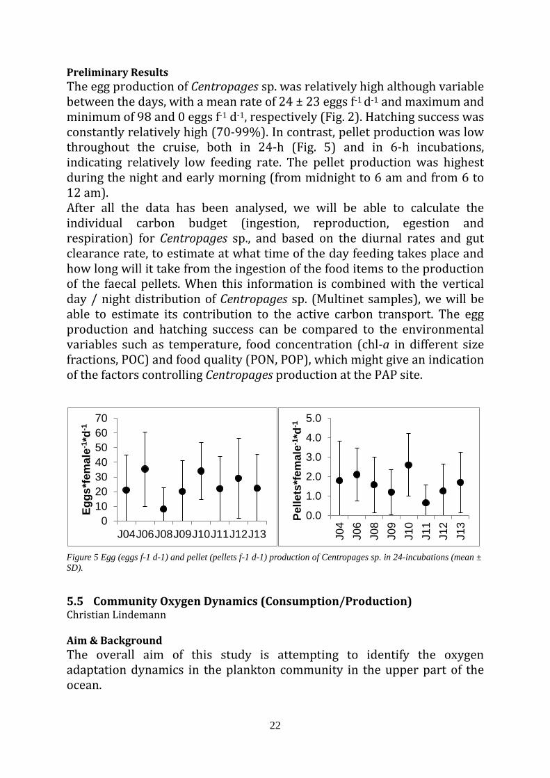
Preliminary Results The egg production of Centropages sp. was relatively high although variable between the days, with a mean rate of 24 ± 23 eggs f-1 d-1 and maximum and minimum of 98 and 0 eggs f-1 d-1, respectively (Fig. 2). Hatching success was constantly relatively high (70-99%). In contrast, pellet production was low throughout the cruise, both in 24-h (Fig. 5) and in 6-h incubations, indicating relatively low feeding rate. The pellet production was highest during the night and early morning (from midnight to 6 am and from 6 to 12 am). After all the data has been analysed, we will be able to calculate the individual carbon budget (ingestion, reproduction, egestion and respiration) for Centropages sp., and based on the diurnal rates and gut clearance rate, to estimate at what time of the day feeding takes place and how long will it take from the ingestion of the food items to the production of the faecal pellets. When this information is combined with the vertical day / night distribution of Centropages sp. (Multinet samples), we will be able to estimate its contribution to the active carbon transport. The egg production and hatching success can be compared to the environmental variables such as temperature, food concentration (chl-a in different size fractions, POC) and food quality (PON, POP), which might give an indication of the factors controlling Centropages production at the PAP site.

Figure 5 Egg (eggs f-1 d-1) and pellet (pellets f-1 d-1) production of Centropages sp. in 24-incubations (mean ± SD).

5.5 Community Oxygen Dynamics (Consumption/Production) Christian Lindemann Aim & Background The overall aim of this study is attempting to identify the oxygen adaptation dynamics in the plankton community in the upper part of the ocean.

010203040506070

J04J06J08J09J10J11J12J13

Eggs

*fem

ale-

1 *d-

1

0.0

1.0

2.0

3.0

4.0

5.0

J04

J06

J08

J09

J10

J11

J12

J13

Pelle

ts*f

emal

e-1*d

-1

23

Community respiration can serve as an indicator of heterotrophic activity. As such it can help to indicate the strength of regenerate production, especially in combination with primary production estimates, from for example carbon based estimates. In modelling studies respiratory rates are often given a fixed (sometimes arbitrary value), like for example 5% per day. To improve this very simple parameter studies about changing community respiration rates can of great use. Phytoplankton dark respiration depends not only changes on temperature and life stage, but a linear relationship between light and dark respiration has also been shown. Together with carbon or nitrogen based primary production rates there is the potential of accessing variability in phytoplankton dark respiration rates. During the RRS James Cook JC 087 two different setups where used. Setup I was designed to test the adaptation response of community respiratory rates towards different light levels. In Setup II 24 hour incubations were measured contentiously to in order to investigate the dial cycle of oxygen dynamics. A closer description of the setup can be found under Material and Method. Material and Methods General Method Water samples were taken using Niskins bottles from 'pre-dawn' CTD casts (unless indicated differently in Table 5). To estimate community respiration rates, water from different depth was incubated in 500 ml glass bottles. The bottles were kept in a flow-through water bath (incubator) on deck with a constant inflow of surface water, thus ensuring realistic temperature and preventing the incubation from heating. The oxygen concentration was measured using the oxygen microsensor system (UNISENSE). All samples where filtered through a 200 µm mesh size net before the incubation, so that potential biases from larger zooplankton were excluded. Method Setup I Water from 200 m depth, within the mixed layer and the surface was incubated into bottles which were either completely darkened (simulating large depth, in this case 200 m), covered with (simulating 20% surface light level) and without any cover (simulating surface water). A list of the CTD's used is presented in Table 5. Water from each depth was incubated in each of the three different treatments, thus all three by three combinations were accounted for. For each of the nine combinations triplicates were made. It was found during the second CTD that was used, that the workload was has

24

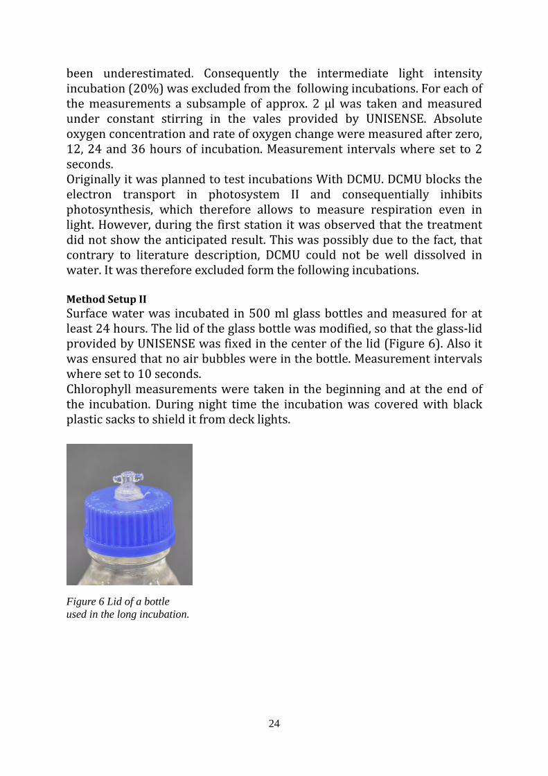
been underestimated. Consequently the intermediate light intensity incubation (20%) was excluded from the following incubations. For each of the measurements a subsample of approx. 2 µl was taken and measured under constant stirring in the vales provided by UNISENSE. Absolute oxygen concentration and rate of oxygen change were measured after zero, 12, 24 and 36 hours of incubation. Measurement intervals where set to 2 seconds. Originally it was planned to test incubations With DCMU. DCMU blocks the electron transport in photosystem II and consequentially inhibits photosynthesis, which therefore allows to measure respiration even in light. However, during the first station it was observed that the treatment did not show the anticipated result. This was possibly due to the fact, that contrary to literature description, DCMU could not be well dissolved in water. It was therefore excluded form the following incubations. Method Setup II Surface water was incubated in 500 ml glass bottles and measured for at least 24 hours. The lid of the glass bottle was modified, so that the glass-lid provided by UNISENSE was fixed in the center of the lid (Figure 6). Also it was ensured that no air bubbles were in the bottle. Measurement intervals where set to 10 seconds. Chlorophyll measurements were taken in the beginning and at the end of the incubation. During night time the incubation was covered with black plastic sacks to shield it from deck lights.

Figure 6 Lid of a bottle used in the long incubation.

25

Table 5 Stations from which water has been used for incubations. Preliminary results

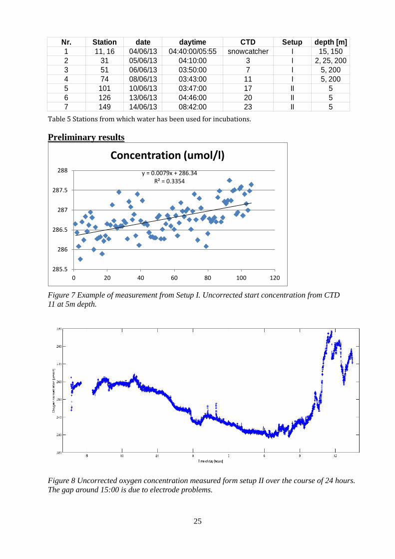
Figure 7 Example of measurement from Setup I. Uncorrected start concentration from CTD 11 at 5m depth.

y = 0.0079x + 286.34 R² = 0.3354

285.5

286

286.5

287

287.5

288

0 20 40 60 80 100 120

Concentration (umol/l)

Nr. Station date daytime CTD Setup depth [m]1 11, 16 04/06/13 04:40:00/05:55 snowcatcher I 15, 1502 31 05/06/13 04:10:00 3 I 2, 25, 2003 51 06/06/13 03:50:00 7 I 5, 2004 74 08/06/13 03:43:00 11 I 5, 2005 101 10/06/13 03:47:00 17 II 56 126 13/06/13 04:46:00 20 II 57 149 14/06/13 08:42:00 23 II 5

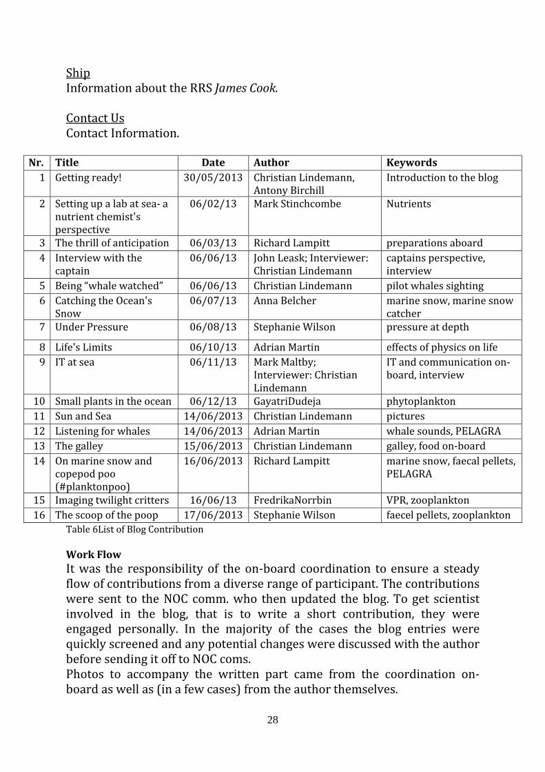
Figure 8 Uncorrected oxygen concentration measured form setup II over the course of 24 hours. The gap around 15:00 is due to electrode problems.

26

5.6 Blog “Down to the Twilight Zone” Christian Lindemann http://downtothetwilightzone.noc.ac.uk/http://downtothetwilightzone.blogspot.com

Aim The main objective of the blog is to communicate the science and life on-board the RRS James Cook during the JC087 cruise. It is meant to reach the general public, other researcher as well as friend and family of the people involved the cruise. Therefore all contributions are written in a language understandable to the general public. It includes (1) scientifically orientated contribution and (2) contribution about life and work on-board. Blog Setup The blog was set up prior to the cruise by the NOC communication department (Robert Curry, Kim Marshall-Brown) (hereafter referred to NOC comm.). The information in the categories “About”, “Science” and “Equipment” was provided by Chief scientist Prof. Richard S. Lampitt prior to the cruise. Information in all other categories was provided by NOC comm.. The text on the site board was written by Ivo Grigorov (DTU Aqua, Charlottenlund, Denmark). To facilitate engagement of scientists during the cruise the two-page document “DOWN to the TWILIGHT ZONE Cruise blog and iReports” (developed by Ivo Grigorov) was send to all participant via email and distributed in laminated copies around the laboratories on the ship. It included advice and suggestion on how to write a good story as well as instructions on how to make iReports. A facebookfanpage (“Down to the Twilight Zone - Expedition”) was set up, to increase outreach towards the facebook community. The facebookfanpage mirrored the blog. It was frequently updated by Antony Birchill. Blog Structure The blog is structured into different main categories as described below.

27

Home The main category of the blog where the different contributions are posted; a list of all the post can be found in Table 6. About General introduction about the twilight zone and the cruise, including a link to the Eurosites page of the PAP site (http://www.eurosites.info/pap/data.php). This information was provided by Chief scientist Prof Richard S Lampitt prior to the cruise. People A list of all the Scientists who participated in the JC087 cruise; it includes a Photo and a short description, written by the respective scientist, about their background and their work during the cruise. Location Information about the PAP site. Science An overview about the science which takes place during the cruise; this information was provided by Chief scientist Prof Richard S Lampitt prior to the cruise. Equipment A short description of the main scientific tools employed during this cruise. This information was provided by Chief scientist Prof Richard S Lampitt prior to the cruise. Media An account of the different media, related to this expedition. • twitter (hashtags #planktonpoo; #MarineSnow) media coverage of the cruise; livescience.com and nbcnews.com have reported on the cruise (as of 17/06/2013 10:15AM)link to the blog of the related EURO-BASIN deep convection cruise (http://deepconvectioncruise.wordpress.com/) Flickr count of the National Oceanographic Centre (NOC) http://www.flickr.com/photos/nationaloceanographycentre/sets/7

2157633911702526/ • Bathysnap movie of activity at the PAP site during 2011/2012 • link to the EURO-BASIN cruise campaign calendar

28

Ship Information about the RRS James Cook. Contact Us Contact Information.

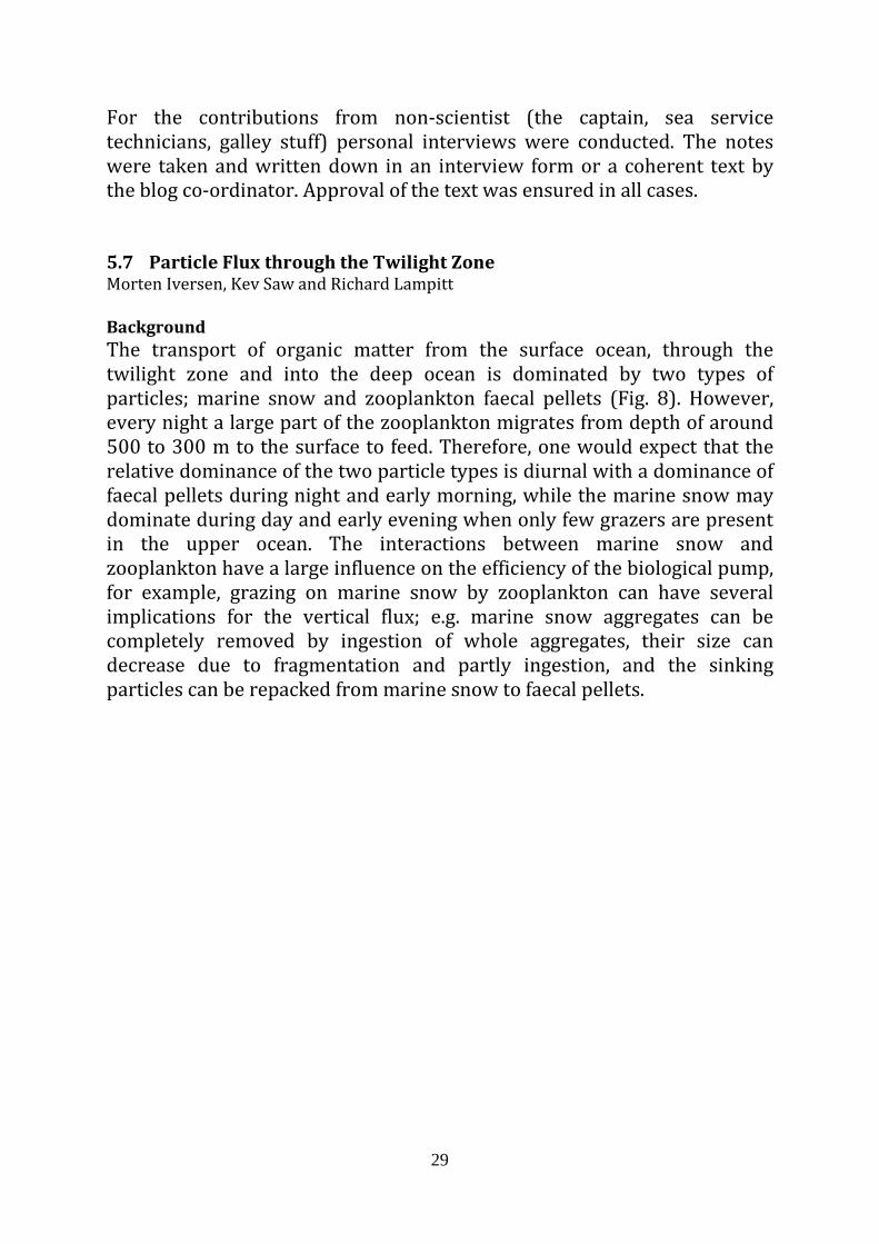
Table 6List of Blog Contribution Work Flow It was the responsibility of the on-board coordination to ensure a steady flow of contributions from a diverse range of participant. The contributions were sent to the NOC comm. who then updated the blog. To get scientist involved in the blog, that is to write a short contribution, they were engaged personally. In the majority of the cases the blog entries were quickly screened and any potential changes were discussed with the author before sending it off to NOC coms. Photos to accompany the written part came from the coordination on-board as well as (in a few cases) from the author themselves.

Nr. Title Date Author Keywords 1 Getting ready! 30/05/2013 Christian Lindemann,

Antony Birchill Introduction to the blog

2 Setting up a lab at sea- a nutrient chemist's perspective

06/02/13 Mark Stinchcombe Nutrients

3 The thrill of anticipation 06/03/13 Richard Lampitt preparations aboard 4 Interview with the

captain 06/06/13 John Leask; Interviewer:

Christian Lindemann captains perspective, interview

5 Being “whale watched” 06/06/13 Christian Lindemann pilot whales sighting 6 Catching the Ocean's

Snow 06/07/13 Anna Belcher marine snow, marine snow

catcher 7 Under Pressure 06/08/13 Stephanie Wilson pressure at depth

8 Life's Limits 06/10/13 Adrian Martin effects of physics on life 9 IT at sea 06/11/13 Mark Maltby;

Interviewer: Christian Lindemann

IT and communication on-board, interview

10 Small plants in the ocean 06/12/13 GayatriDudeja phytoplankton 11 Sun and Sea 14/06/2013 Christian Lindemann pictures 12 Listening for whales 14/06/2013 Adrian Martin whale sounds, PELAGRA 13 The galley 15/06/2013 Christian Lindemann galley, food on-board 14 On marine snow and

copepod poo (#planktonpoo)

16/06/2013 Richard Lampitt marine snow, faecal pellets, PELAGRA

15 Imaging twilight critters 16/06/13 FredrikaNorrbin VPR, zooplankton 16 The scoop of the poop 17/06/2013 Stephanie Wilson faecel pellets, zooplankton

29

For the contributions from non-scientist (the captain, sea service technicians, galley stuff) personal interviews were conducted. The notes were taken and written down in an interview form or a coherent text by the blog co-ordinator. Approval of the text was ensured in all cases. 5.7 Particle Flux through the Twilight Zone Morten Iversen, Kev Saw and Richard Lampitt Background The transport of organic matter from the surface ocean, through the twilight zone and into the deep ocean is dominated by two types of particles; marine snow and zooplankton faecal pellets (Fig. 8). However, every night a large part of the zooplankton migrates from depth of around 500 to 300 m to the surface to feed. Therefore, one would expect that the relative dominance of the two particle types is diurnal with a dominance of faecal pellets during night and early morning, while the marine snow may dominate during day and early evening when only few grazers are present in the upper ocean. The interactions between marine snow and zooplankton have a large influence on the efficiency of the biological pump, for example, grazing on marine snow by zooplankton can have several implications for the vertical flux; e.g. marine snow aggregates can be completely removed by ingestion of whole aggregates, their size can decrease due to fragmentation and partly ingestion, and the sinking particles can be repacked from marine snow to faecal pellets.

30

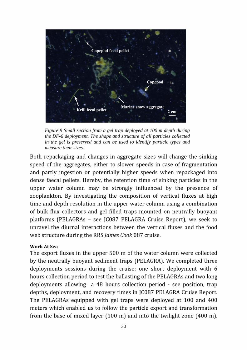
Figure 9 Small section from a gel trap deployed at 100 m depth during the DF-6 deployment. The shape and structure of all particles collected in the gel is preserved and can be used to identify particle types and measure their sizes.

Both repackaging and changes in aggregate sizes will change the sinking speed of the aggregates, either to slower speeds in case of fragmentation and partly ingestion or potentially higher speeds when repackaged into dense faecal pellets. Hereby, the retention time of sinking particles in the upper water column may be strongly influenced by the presence of zooplankton. By investigating the composition of vertical fluxes at high time and depth resolution in the upper water column using a combination of bulk flux collectors and gel filled traps mounted on neutrally buoyant platforms (PELAGRAs – see JC087 PELAGRA Cruise Report), we seek to unravel the diurnal interactions between the vertical fluxes and the food web structure during the RRS James Cook 087 cruise.

Work At Sea The export fluxes in the upper 500 m of the water column were collected by the neutrally buoyant sediment traps (PELAGRA). We completed three deployments sessions during the cruise; one short deployment with 6 hours collection period to test the ballasting of the PELAGRAs and two long deployments allowing a 48 hours collection period - see position, trap depths, deployment, and recovery times in JC087 PELAGRA Cruise Report. The PELAGRAs equipped with gel traps were deployed at 100 and 400 meters which enabled us to follow the particle export and transformation from the base of mixed layer (100 m) and into the twilight zone (400 m).

31

On those PELAGRAs two funnel-collectors captured biogeochemical mass fluxes of carbon, nitrogen, biogenic opal, calcium carbonate and lithogenic material while the two traps without funnels were equipped with viscous gel which preserved the sinking material in its original shape. The different particle types collected in the gel were photographed on board using a digital camera and will be used to create particle size distribution and abundance of the flux. The combination of several deployments collecting either during a 24 h period or timed to only collect the night or day fluxes will hopefully provide quantitative and qualitative information on the origin of sinking particles and processes important for the flux attenuation on a diurnal time scale.

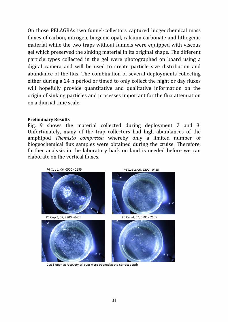
Preliminary Results Fig. 9 shows the material collected during deployment 2 and 3. Unfortunately, many of the trap collectors had high abundances of the amphipod Themisto compressa whereby only a limited number of biogeochemical flux samples were obtained during the cruise. Therefore, further analysis in the laboratory back on land is needed before we can elaborate on the vertical fluxes.

32

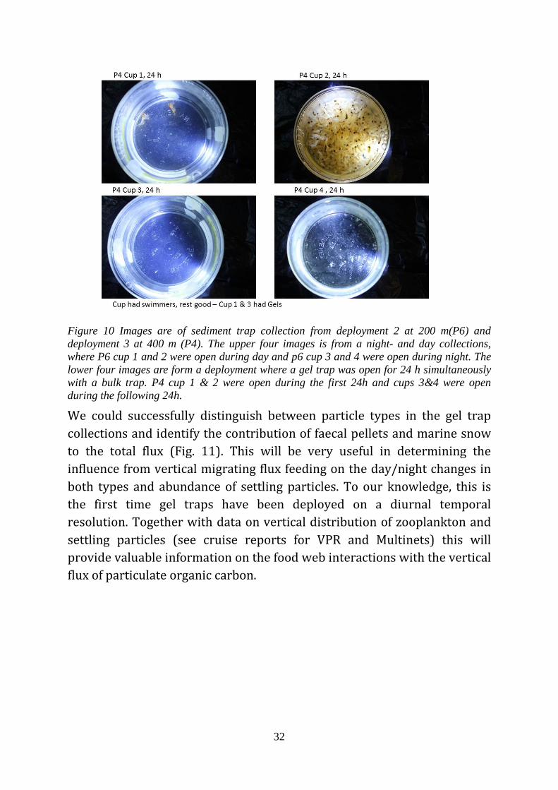
Figure 10 Images are of sediment trap collection from deployment 2 at 200 m(P6) and deployment 3 at 400 m (P4). The upper four images is from a night- and day collections, where P6 cup 1 and 2 were open during day and p6 cup 3 and 4 were open during night. The lower four images are form a deployment where a gel trap was open for 24 h simultaneously with a bulk trap. P4 cup 1 & 2 were open during the first 24h and cups 3&4 were open during the following 24h.

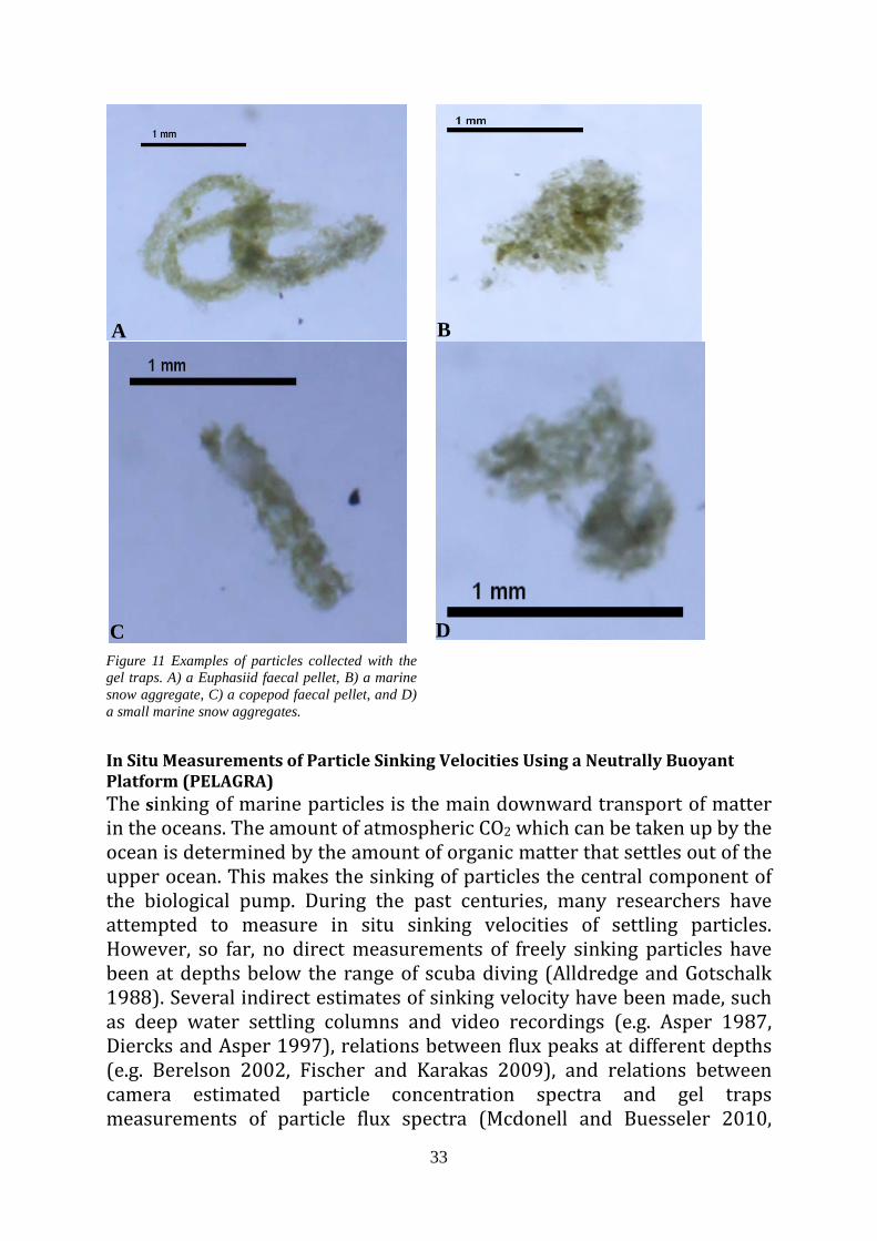
We could successfully distinguish between particle types in the gel trap collections and identify the contribution of faecal pellets and marine snow to the total flux (Fig. 11). This will be very useful in determining the influence from vertical migrating flux feeding on the day/night changes in both types and abundance of settling particles. To our knowledge, this is the first time gel traps have been deployed on a diurnal temporal resolution. Together with data on vertical distribution of zooplankton and settling particles (see cruise reports for VPR and Multinets) this will provide valuable information on the food web interactions with the vertical flux of particulate organic carbon.

33

Figure 11 Examples of particles collected with the gel traps. A) a Euphasiid faecal pellet, B) a marine snow aggregate, C) a copepod faecal pellet, and D) a small marine snow aggregates.

In Situ Measurements of Particle Sinking Velocities Using a Neutrally Buoyant Platform (PELAGRA) The sinking of marine particles is the main downward transport of matter in the oceans. The amount of atmospheric CO2 which can be taken up by the ocean is determined by the amount of organic matter that settles out of the upper ocean. This makes the sinking of particles the central component of the biological pump. During the past centuries, many researchers have attempted to measure in situ sinking velocities of settling particles. However, so far, no direct measurements of freely sinking particles have been at depths below the range of scuba diving (Alldredge and Gotschalk 1988). Several indirect estimates of sinking velocity have been made, such as deep water settling columns and video recordings (e.g. Asper 1987, Diercks and Asper 1997), relations between flux peaks at different depths (e.g. Berelson 2002, Fischer and Karakas 2009), and relations between camera estimated particle concentration spectra and gel traps measurements of particle flux spectra (Mcdonell and Buesseler 2010,

A B

C D

34

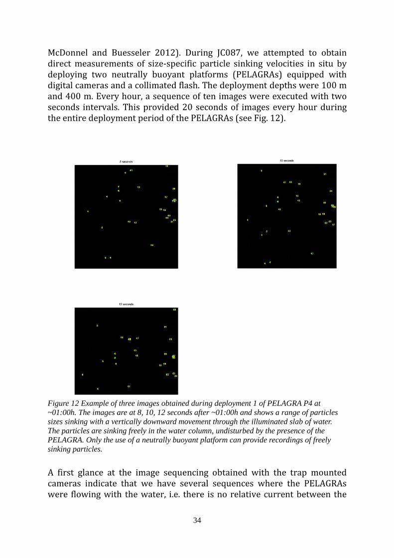
McDonnel and Buesseler 2012). During JC087, we attempted to obtain direct measurements of size-specific particle sinking velocities in situ by deploying two neutrally buoyant platforms (PELAGRAs) equipped with digital cameras and a collimated flash. The deployment depths were 100 m and 400 m. Every hour, a sequence of ten images were executed with two seconds intervals. This provided 20 seconds of images every hour during the entire deployment period of the PELAGRAs (see Fig. 12).

A first glance at the image sequencing obtained with the trap mounted cameras indicate that we have several sequences where the PELAGRAs were flowing with the water, i.e. there is no relative current between the

Figure 12 Example of three images obtained during deployment 1 of PELAGRA P4 at ~01:00h. The images are at 8, 10, 12 seconds after ~01:00h and shows a range of particles sizes sinking with a vertically downward movement through the illuminated slab of water. The particles are sinking freely in the water column, undisturbed by the presence of the PELAGRA. Only the use of a neutrally buoyant platform can provide recordings of freely sinking particles.

35

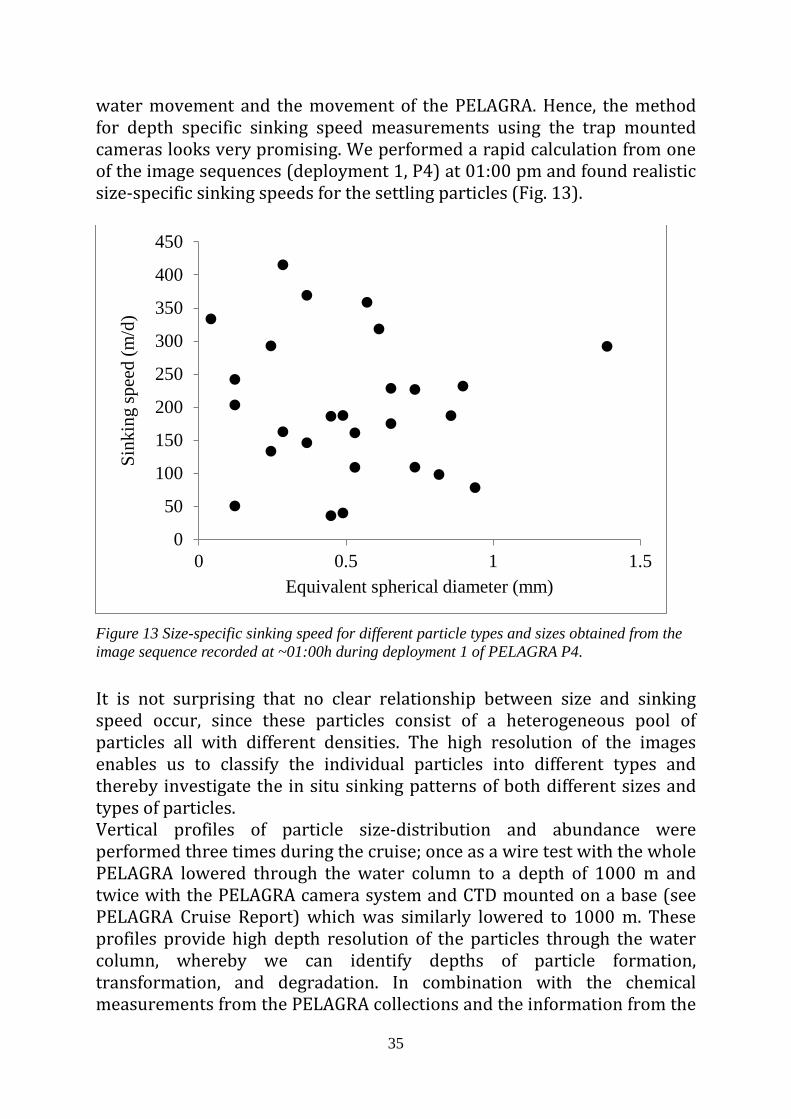
water movement and the movement of the PELAGRA. Hence, the method for depth specific sinking speed measurements using the trap mounted cameras looks very promising. We performed a rapid calculation from one of the image sequences (deployment 1, P4) at 01:00 pm and found realistic size-specific sinking speeds for the settling particles (Fig. 13).

Figure 13 Size-specific sinking speed for different particle types and sizes obtained from the image sequence recorded at ~01:00h during deployment 1 of PELAGRA P4.

It is not surprising that no clear relationship between size and sinking speed occur, since these particles consist of a heterogeneous pool of particles all with different densities. The high resolution of the images enables us to classify the individual particles into different types and thereby investigate the in situ sinking patterns of both different sizes and types of particles. Vertical profiles of particle size-distribution and abundance were performed three times during the cruise; once as a wire test with the whole PELAGRA lowered through the water column to a depth of 1000 m and twice with the PELAGRA camera system and CTD mounted on a base (see PELAGRA Cruise Report) which was similarly lowered to 1000 m. These profiles provide high depth resolution of the particles through the water column, whereby we can identify depths of particle formation, transformation, and degradation. In combination with the chemical measurements from the PELAGRA collections and the information from the

0

50

100

150

200

250

300

350

400

450

0 0.5 1 1.5

Sink

ing

spee

d (m

/d)

Equivalent spherical diameter (mm)

36

gel traps, these profiles will be valuable tool to identify important depth specific processes for the efficiency of the biological pump. Direct measurements of sinking speed and microbial community respiration of different types of faecal pellets were performed on board to estimate the microbial degradation and export of faecal pellets from salps, Themisto compressa, and Pleuromamma sp.. We observed sinking speeds of salp pellets between 200 and 500 m d-1, while T. compressa pellets on sank with an average speed of around 150 m d-1. However, we cannot conclude from the sinking speed alone which pellet type is most likely to reach the deep ocean, since both the rate of microbial degradation and grazing from higher trophic levels have a large impact on the attenuation of their export fluxes. Alldredge, A., and Gotschalk, C.: In situ settling behavior of marine snow, Limnol. Oceanogr., 33, 339-351, 1988. Asper, V. L.: Measuring the flux and sinking speed of marine snow aggregates., Deep-Sea Res., 34, 1-17, 1987. Berelson, W. M.: Particle settling rates increase with depth on the ocean, Deep-Sea Res. II, 49, 237-251, 2002. Diercks, A. R., and Asper, V. L.: In situ settling speeds of marine snow aggregates below the mixed layer: Black Sea and Gulf of Mexico, Deep-Sea Res I, 44, 385-398, 1997. Fischer, G., and Karakas, G.: Sinking rates and ballast composition of particles in the Atlantic Ocean: implications for the organic carbon fluxes to the deep ocean, Biogeosciences, 6, 85-102, 2009. McDonnell, A. M. P., and Buesseler, K. O.: A new method for the estimation of sinking particle fluxes from measurements of the particle size distribution, average sinking velocity, and carbon content, Limnol. Oceanogr. Methods, 10, 329-346, 2012. McDonnell, A. M. P., and Buesseler, K. O.: Variability in the average sinking velocities of marine particles, Limnol. Oceanogr., 55, doi:10.4319/lo.2010.4355.4315.0000, 2010. 5.8 Molecular Variation of Lipids in Particles Blazenka Gasparovic Scientific Motivation Lipids are essential for every living organism as they play vital roles in the membrane composition and the regulation of metabolic processes. They represent the carbon rich organic matter with very high energetic value, thus being an important metabolic fuel. Lipids differ in their chemical structure to a substantial degree and contain different functional groups

37

influencing their reactivity. However, molecular structure is not the only factor relevant for organic matter reactivity, the fate of which also depends on environmental conditions. The main origin of lipids is phytoplankton, as well as autotrophic bacteria and in much lesser extent heterotrophic bacteria. Plankton is constantly challenged with various abiotic stresses (light intensity, temperature, and nutrient availability) in their natural environment. Characterization of marine lipids on a molecular level enables their use as good geochemical markers for the identification of different sources and processes of organic matter in the sea. For example, polar lipids are plankton biomembrane structure components, glycolipids are located predominantly in photosynthetic membranes and indicate on presence of autotrophs, triacylglycerols indicate plankton metabolic reserves, mono- and di-acylglycerides and free fatty acids breakdown products and characterize organic matter degradation level.

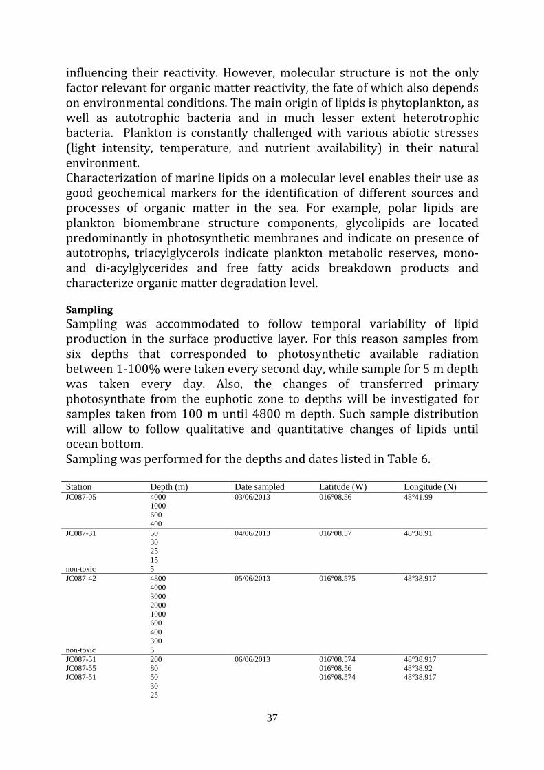
Sampling Sampling was accommodated to follow temporal variability of lipid production in the surface productive layer. For this reason samples from six depths that corresponded to photosynthetic available radiation between 1-100% were taken every second day, while sample for 5 m depth was taken every day. Also, the changes of transferred primary photosynthate from the euphotic zone to depths will be investigated for samples taken from 100 m until 4800 m depth. Such sample distribution will allow to follow qualitative and quantitative changes of lipids until ocean bottom. Sampling was performed for the depths and dates listed in Table 6. Station Depth (m) Date sampled Latitude (W) Longitude (N) JC087-05 4000 03/06/2013 016°08.56 48°41.99 1000 600 400 JC087-31 50 04/06/2013 016°08.57 48°38.91 30 25 15 non-toxic 5 JC087-42 4800 05/06/2013 016°08.575 48°38.917 4000 3000 2000 1000 600 400 300 non-toxic 5 JC087-51 200 06/06/2013 016°08.574 48°38.917 JC087-55 80 016°08.56 48°38.92 JC087-51 50 016°08.574 48°38.917 30 25

38

15 5 surface non-toxic 5 07/06/2013 016°08.56 48°38.92 JC087-74 200 08/06/2013 016°08.604 48°38.919 100 50 30 25 15 5 JC087-75 surface 016°29.30 48°39.04 non-toxic 5 09/06/2013 016°08.56 48°38.92 JC087-101 200 10/06/2013 016°08.57 48°38.92 100 50 30 25 15 5 JC087-104 surface 016°08.57 48°38.91 non-toxic 5 11/06/2013 016°08.56 48°38.92 JC087-126 200 13/06/2013 016°08.57 48°38.91 100 50 30 25 15 5 JC087-130 surface 016°08.57 48°38.92 JC087-151 4800 14/06/2013 016°08.58 48°38.91 4500 4000 3500 3000 2500 2000 1500 1000 800 600 400 300 5 Table 7 Pre-treatment on Board For particulate lipid determination seawater was filtered through 0.7 µm Whatman GF/F filters pre-burned at 450ºC/5 h. For the surface productive layer (depths 0-50 m) 4 to 5 l of seawater was filtered, while 9 to 11 l of deep seawater (depths 200-4800 m) was filtered. Filters are stored at -80°C until the particulate lipid extraction. Further Work Lipids from the collected particles will be extracted by a one-phase solvent mixture of dichloromethane-methanol-water. Ten micrograms of internal standard n-hexadecanone will be added to each sample before the extraction for the estimation of lipid recovery. Extracts will be concentrated under a nitrogen atmosphere and stored at -20 ºC until measurements.

39

The extracts will be analyzed for lipid classes by a thin-layer chromatography. Eighteen lipid classes (hydrocarbons, wax and steryl esters, fatty acid methyl esters, ketone, triacylglycerols, free fatty acids, alcohols, 1,3-diacylglycerols, sterols, 1,2-diacylglycerols, pigments, monoacylglycerols, mono- and di-galactosyldiacylglycerols, sulfoquinovosyldiacylglycerol, mono- and di-phosphatidylglycerols, phosphatidylethanolamines, and phosphatidylcholine) will be quantified. Also, intact polar diacylglycerolipids will be qualified and quentified by high performance liquid chromatography/electrospray ionization–mass spectrometry. This method determines three classes of phospholipids, three classes of betaine lipids and three classes of glycolipids. If we will have enough samples after first two analysis samples will be analyzed with Fourier transform ion cyclotron resonance mass spectrometry with electrospray ionization. This method distinguishes thousands of compounds of different elemental compositions. Scientific Outcomes Investigations of marine organic matter are becoming more popular since carbon capture and sequestration is a possible method of reducing the atmospheric carbon dioxide level. Therefore, studies of OM concentration, production, characterization, cycling and distribution, as well as influential factors, are important. Lipids are good candidates for such studies due to their stable nature compared to carbohydrates and proteins. To contribute to this important issue several major questions were addressed for this cruise. First, what are the compositional changes in the particulate lipid pool in the surface productive layer during the investigated period? How varying environmental conditions influenced lipid production and composition? Which plankton group influenced the most lipid quantity? It is expected that at low nutrient conditions more glycolipids, molecules without nitrogen or phosphorus, would be synthesized instead of phospholipids representing N - or/and P - conserving mechanism. The distributions of intact polar diacylglycerolipids along the cruise transect should provide important new insights on lipid tentative planktonic sources. Second, which are the magnitudes and compositional changes in the molecular characteristics of various lipid classes and individual compounds at various depths until bottom layer? Therefore it is aimed to appoint crucial depths at which N and P are removed from the certain lipid classes. Which are the most stable lipids that are surviving transfer from the euphotic zone to the benthic systems being as such good for CO2 sequestration? It should be elucidated which environmental conditions are responsible for production of those stable lipids.

40

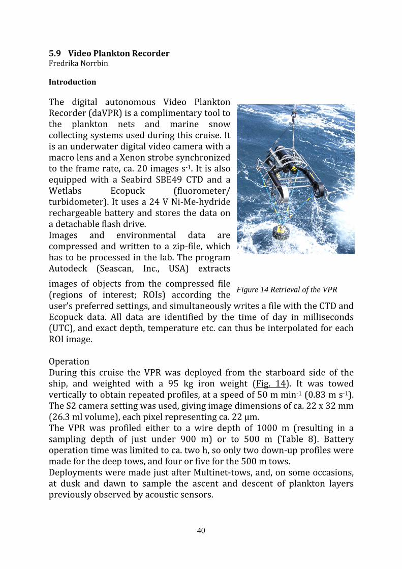
5.9 Video Plankton Recorder Fredrika Norrbin Introduction The digital autonomous Video Plankton Recorder (daVPR) is a complimentary tool to the plankton nets and marine snow collecting systems used during this cruise. It is an underwater digital video camera with a macro lens and a Xenon strobe synchronized to the frame rate, ca. 20 images s-1. It is also equipped with a Seabird SBE49 CTD and a Wetlabs Ecopuck (fluorometer/ turbidometer). It uses a 24 V Ni-Me-hydride rechargeable battery and stores the data on a detachable flash drive. Images and environmental data are compressed and written to a zip-file, which has to be processed in the lab. The program Autodeck (Seascan, Inc., USA) extracts images of objects from the compressed file (regions of interest; ROIs) according the user’s preferred settings, and simultaneously writes a file with the CTD and Ecopuck data. All data are identified by the time of day in milliseconds (UTC), and exact depth, temperature etc. can thus be interpolated for each ROI image. Operation During this cruise the VPR was deployed from the starboard side of the ship, and weighted with a 95 kg iron weight (Fig. 14). It was towed vertically to obtain repeated profiles, at a speed of 50 m min-1 (0.83 m s-1). The S2 camera setting was used, giving image dimensions of ca. 22 x 32 mm (26.3 ml volume), each pixel representing ca. 22 µm. The VPR was profiled either to a wire depth of 1000 m (resulting in a sampling depth of just under 900 m) or to 500 m (Table 8). Battery operation time was limited to ca. two h, so only two down-up profiles were made for the deep tows, and four or five for the 500 m tows. Deployments were made just after Multinet-tows, and, on some occasions, at dusk and dawn to sample the ascent and descent of plankton layers previously observed by acoustic sensors.

Figure 14 Retrieval of the VPR

41

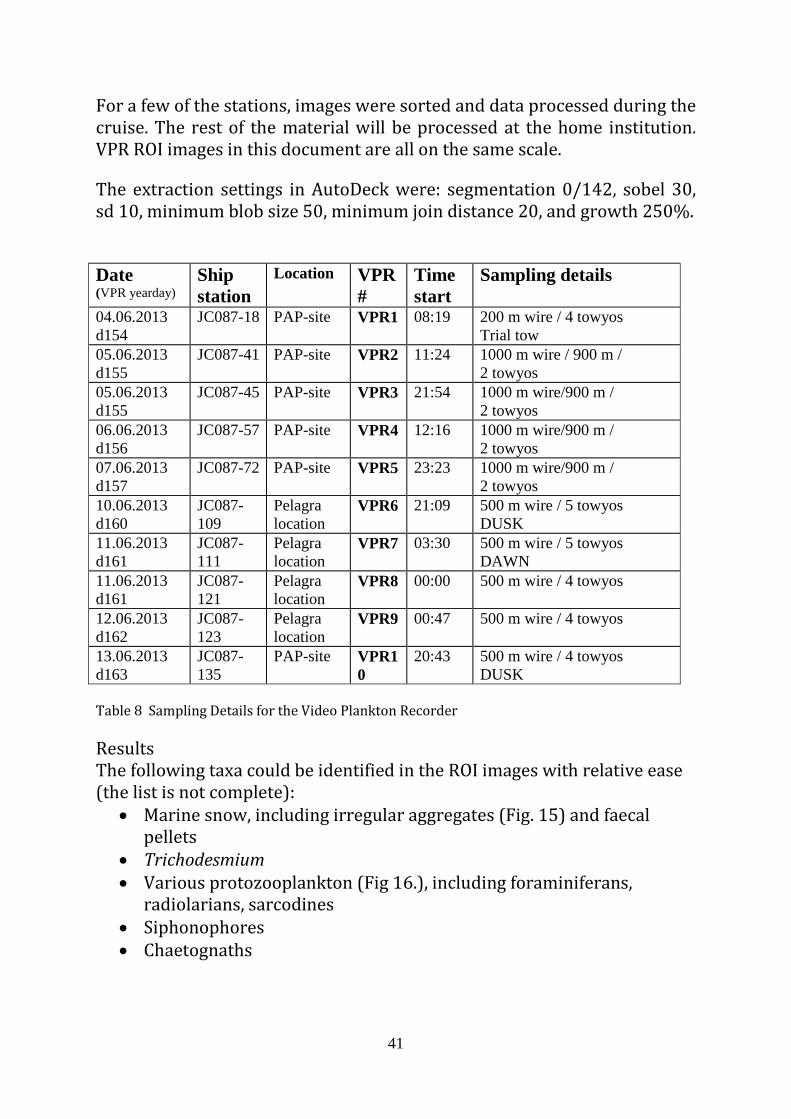
For a few of the stations, images were sorted and data processed during the cruise. The rest of the material will be processed at the home institution. VPR ROI images in this document are all on the same scale. The extraction settings in AutoDeck were: segmentation 0/142, sobel 30, sd 10, minimum blob size 50, minimum join distance 20, and growth 250%.

Table 8 Sampling Details for the Video Plankton Recorder Results The following taxa could be identified in the ROI images with relative ease (the list is not complete):

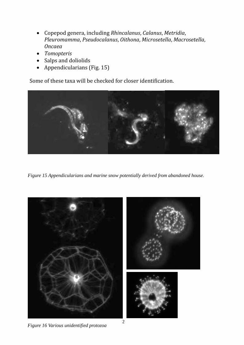
• Marine snow, including irregular aggregates (Fig. 15) and faecal pellets

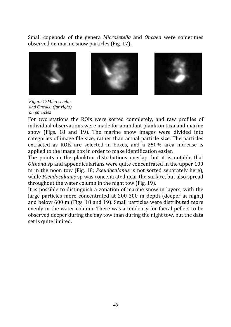
• Trichodesmium • Various protozooplankton (Fig 16.), including foraminiferans,

radiolarians, sarcodines • Siphonophores • Chaetognaths

Date (VPR yearday)

Ship station

Location VPR #

Time start

Sampling details

04.06.2013 d154

JC087-18 PAP-site VPR1 08:19 200 m wire / 4 towyos Trial tow

05.06.2013 d155

JC087-41 PAP-site VPR2 11:24 1000 m wire / 900 m / 2 towyos

05.06.2013 d155

JC087-45 PAP-site VPR3 21:54 1000 m wire/900 m / 2 towyos

06.06.2013 d156

JC087-57 PAP-site VPR4 12:16 1000 m wire/900 m / 2 towyos

07.06.2013 d157

JC087-72 PAP-site VPR5 23:23 1000 m wire/900 m / 2 towyos

10.06.2013 d160

JC087-109

Pelagra location

VPR6 21:09 500 m wire / 5 towyos DUSK

11.06.2013 d161

JC087-111

Pelagra location

VPR7 03:30 500 m wire / 5 towyos DAWN

11.06.2013 d161

JC087-121

Pelagra location

VPR8 00:00 500 m wire / 4 towyos

12.06.2013 d162

JC087-123

Pelagra location

VPR9 00:47 500 m wire / 4 towyos

13.06.2013 d163

JC087-135

PAP-site VPR10

20:43 500 m wire / 4 towyos DUSK

42

• Copepod genera, including Rhincalanus, Calanus, Metridia, Pleuromamma, Pseudocalanus, Oithona, Microsetella, Macrosetella, Oncaea

• Tomopteris • Salps and doliolids • Appendicularians (Fig. 15)

Some of these taxa will be checked for closer identification.

Figure 15 Appendicularians and marine snow potentially derived from abandoned house.

Figure 16 Various unidentified protozoa

43

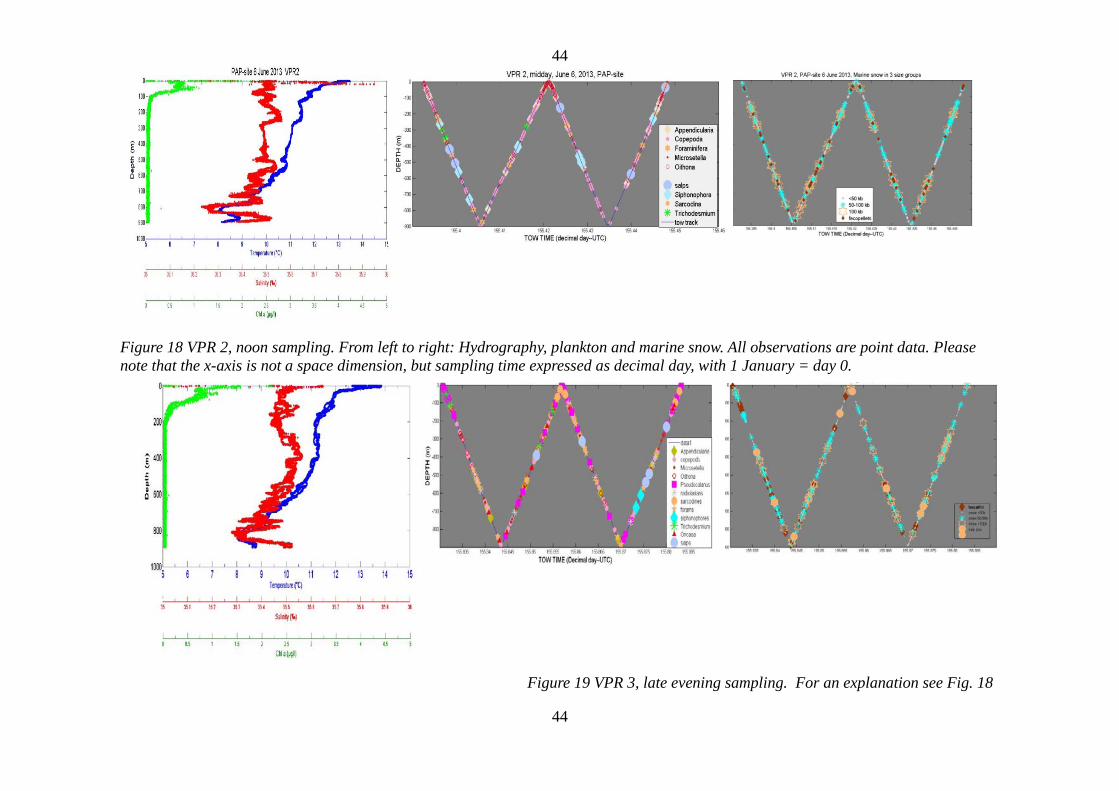
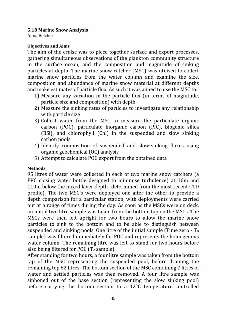
Small copepods of the genera Microsetella and Oncaea were sometimes observed on marine snow particles (Fig. 17). For two stations the ROIs were sorted completely, and raw profiles of individual observations were made for abundant plankton taxa and marine snow (Figs. 18 and 19). The marine snow images were divided into categories of image file size, rather than actual particle size. The particles extracted as ROIs are selected in boxes, and a 250% area increase is applied to the image box in order to make identification easier. The points in the plankton distributions overlap, but it is notable that Oithona sp and appendicularians were quite concentrated in the upper 100 m in the noon tow (Fig. 18; Pseudocalanus is not sorted separately here), while Pseudocalanus sp was concentrated near the surface, but also spread throughout the water column in the night tow (Fig. 19). It is possible to distinguish a zonation of marine snow in layers, with the large particles more concentrated at 200-300 m depth (deeper at night) and below 600 m (Figs. 18 and 19). Small particles were distributed more evenly in the water column. There was a tendency for faecal pellets to be observed deeper during the day tow than during the night tow, but the data set is quite limited.

Figure 17Microsetella and Oncaea (far right) on particles

44

44

Figure 18 VPR 2, noon sampling. From left to right: Hydrography, plankton and marine snow. All observations are point data. Please note that the x-axis is not a space dimension, but sampling time expressed as decimal day, with 1 January = day 0.

Figure 19 VPR 3, late evening sampling. For an explanation see Fig. 18

45

5.10 Marine Snow Analysis Anna Belcher Objectives and Aims The aim of the cruise was to piece together surface and export processes, gathering simultaneous observations of the plankton community structure in the surface ocean, and the composition and magnitude of sinking particles at depth. The marine snow catcher (MSC) was utilised to collect marine snow particles from the water column and examine the size, composition and abundance of marine snow material at different depths and make estimates of particle flux. As such it was aimed to use the MSC to:

1) Measure any variation in the particle flux (in terms of magnitude, particle size and composition) with depth

2) Measure the sinking rates of particles to investigate any relationship with particle size

3) Collect water from the MSC to measure the particulate organic carbon (POC), particulate inorganic carbon (PIC), biogenic silica (BSi), and chlorophyll (Chl) in the suspended and slow sinking carbon pools

4) Identify composition of suspended and slow-sinking fluxes using organic geochemical (OC) analysis

5) Attempt to calculate POC export from the obtained data

Methods 95 litres of water were collected in each of two marine snow catchers (a PVC closing water bottle designed to minimise turbulence) at 10m and 110m below the mixed layer depth (determined from the most recent CTD profile). The two MSC’s were deployed one after the other to provide a depth comparison for a particular station, with deployments were carried out at a range of times during the day. As soon as the MSCs were on deck, an initial two litre sample was taken from the bottom tap on the MSCs. The MSCs were then left upright for two hours to allow the marine snow particles to sink to the bottom and to be able to distinguish between suspended and sinking pools. One litre of the initial sample (Time zero - T0 sample) was filtered immediately for POC and represents the homogenous water column. The remaining litre was left to stand for two hours before also being filtered for POC (T2 sample). After standing for two hours, a four litre sample was taken from the bottom tap of the MSC representing the suspended pool, before draining the remaining top 82 litres. The bottom section of the MSC containing 7 litres of water and settled particles was then removed. A four litre sample was siphoned out of the base section (representing the slow sinking pool) before carrying the bottom section to a 12°C temperature controlled

46

laboratory. Water samples collected from both the top and base sections of the MSC were filtered for analysis of POC. PIC, POC, BSi, Chl and OC analysis. Particles that had settled to the base of the bottom chamber were removed using a wide-bore pipette and photographed using a Müller DCM310 microscope camera and Technico XE series microscope. These particles represent the fast sinking pool. In addition, sinking rate experiments using a flow chamber (Ploug and Jørgensen, 1999; Ploug et al., 2010) were carried out on 10-15 particles from each MSC. Each aggregate was carefully placed in a 10cm high Plexiglas tube (5cm diameter), on a net extended across middle of the tube. Flow is supplied from below the net, adjusted using a needle valve, resulting in a uniform flow field across the upper chamber. The flow was adjusted so that the particle is suspended one particle diameter above the net. At this point the sinking velocity is balanced by the upward flow velocity (Ploug et al., 2010), and can be calculated by dividing the flow rate by the area of the flow chamber. Three measurements of the sinking velocity were made for each particle and the x, y, and z dimensions measured using a horizontal dissection microscope with a calibrated ocular. The particles that were sunk were preserved individually in ependorf tubes and stored in a -20°C freezer. Filter Sample Preparation, Preservation and Analysis: POC: Each sample was filtered through a 0.7μm pore size, 25mm diameter, ashed GFF filter, rinsed with milliQ water, placed in a Petri dish, air dried and stored at room temperature for later analysis. PIC: Each sample was filtered through a 0.8μm pore size, 25mm diameter, nucleopore polycarbonate membrane filter, rinsed with milliQ water, stored in a cryotube vial, air dried and stored at room temperature for later analysis. BSi: Each sample was filtered through 0.8μm pore size, 25mm diameter, nucleopore polycarbonate membrane filter, rinsed with milliQ water, stored in a centrifuge tube, air dried and stored at room temperature for later analysis. Chl: Each sample was filtered through at 0.7μm pore size, 25mm diameter, ashed GFF filter, rinsed with milliQ water and placed in a glass vial. 8ml 90% acetone was added and the vial stored in a fridge for 18-20 hours before onboard analysis on a fluorometer. OC: Each sample was filtered through at 0.7μm pore size, 25mm diameter, pre-weighed ashed GFF filters, rinsed with milliQ water, placed foil and stored at -80 °C for later analysis.

47

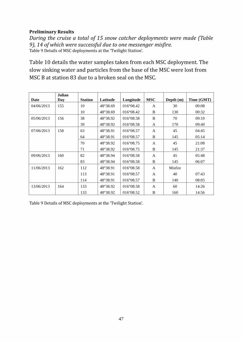
Preliminary Results During the cruise a total of 15 snow catcher deployments were made (Table 9), 14 of which were successful due to one messenger misfire. Table 9 Details of MSC deployments at the ‘Twilight Station’. Table 10 details the water samples taken from each MSC deployment. The slow sinking water and particles from the base of the MSC were lost from MSC B at station 83 due to a broken seal on the MSC.

Date Julian Day Station Latitude Longitude MSC Depth (m) Time (GMT)

04/06/2013 155 10 48°38.69 016°08.42 A 30 00:08 10 48°38.69 016°08.42 B 130 00:32 05/06/2013 156 38 48°38.92 016°08.58 B 70 09:10 39 48°38.92 016°08.58 A 170 09:40 07/06/2013 158 63 48°38.91 016°08.57 A 45 04:45

64 48°38.91 016°08.57 B 145 05:14

70 48°38.92 016°08.75 A 45 21:08 71 48°38.92 016°08.75 B 145 21:37 09/06/2013 160 82 48°38.94 016°08.58 A 45 05:48 83 48°38.94 016°08.58 B 145 06:07 11/06/2013 162 112 48°38.91 016°08.58 A Misfire

113 48°38.91 016°08.57 A 40 07:43 114 48°38.91 016°08.57 B 140 08:05 13/06/2013 164 133 48°38.92 016°08.58 A 60 14:26 133 48°38.92 016°08.52 B 160 14:56

Table 9 Details of MSC deployments at the ‘Twilight Station’.

48

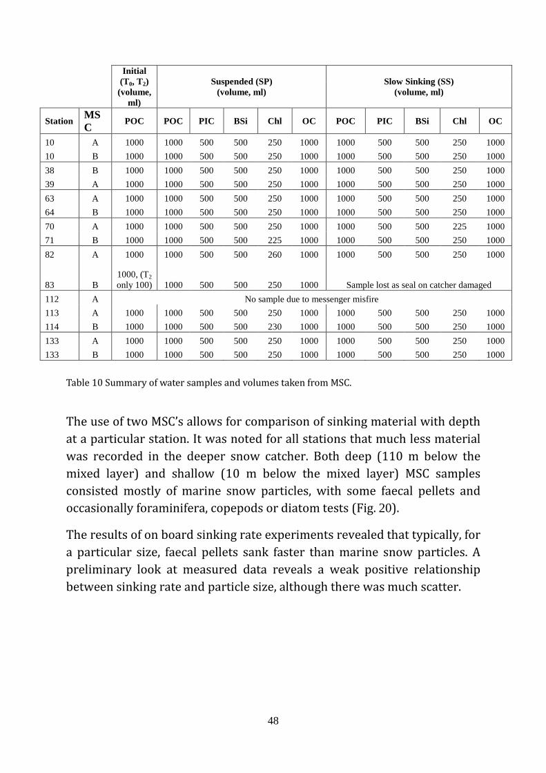
Initial

(T0, T2) (volume,

ml)

Suspended (SP) (volume, ml)

Slow Sinking (SS) (volume, ml)

Station MSC POC POC PIC BSi Chl OC POC PIC BSi Chl OC

10 A 1000 1000 500 500 250 1000 1000 500 500 250 1000 10 B 1000 1000 500 500 250 1000 1000 500 500 250 1000 38 B 1000 1000 500 500 250 1000 1000 500 500 250 1000 39 A 1000 1000 500 500 250 1000 1000 500 500 250 1000 63 A 1000 1000 500 500 250 1000 1000 500 500 250 1000 64 B 1000 1000 500 500 250 1000 1000 500 500 250 1000 70 A 1000 1000 500 500 250 1000 1000 500 500 225 1000 71 B 1000 1000 500 500 225 1000 1000 500 500 250 1000 82 A 1000 1000 500 500 260 1000 1000 500 500 250 1000

83 B 1000, (T2 only 100) 1000 500 500 250 1000 Sample lost as seal on catcher damaged

112 A No sample due to messenger misfire 113 A 1000 1000 500 500 250 1000 1000 500 500 250 1000 114 B 1000 1000 500 500 230 1000 1000 500 500 250 1000 133 A 1000 1000 500 500 250 1000 1000 500 500 250 1000 133 B 1000 1000 500 500 250 1000 1000 500 500 250 1000

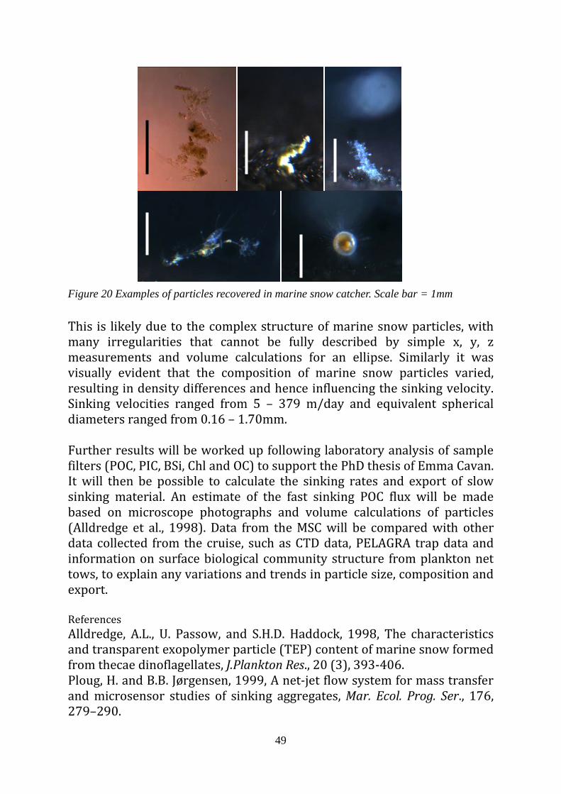
Table 10 Summary of water samples and volumes taken from MSC. The use of two MSC’s allows for comparison of sinking material with depth at a particular station. It was noted for all stations that much less material was recorded in the deeper snow catcher. Both deep (110 m below the mixed layer) and shallow (10 m below the mixed layer) MSC samples consisted mostly of marine snow particles, with some faecal pellets and occasionally foraminifera, copepods or diatom tests (Fig. 20).

The results of on board sinking rate experiments revealed that typically, for a particular size, faecal pellets sank faster than marine snow particles. A preliminary look at measured data reveals a weak positive relationship between sinking rate and particle size, although there was much scatter.

49

Figure 20 Examples of particles recovered in marine snow catcher. Scale bar = 1mm This is likely due to the complex structure of marine snow particles, with many irregularities that cannot be fully described by simple x, y, z measurements and volume calculations for an ellipse. Similarly it was visually evident that the composition of marine snow particles varied, resulting in density differences and hence influencing the sinking velocity. Sinking velocities ranged from 5 – 379 m/day and equivalent spherical diameters ranged from 0.16 – 1.70mm. Further results will be worked up following laboratory analysis of sample filters (POC, PIC, BSi, Chl and OC) to support the PhD thesis of Emma Cavan. It will then be possible to calculate the sinking rates and export of slow sinking material. An estimate of the fast sinking POC flux will be made based on microscope photographs and volume calculations of particles (Alldredge et al., 1998). Data from the MSC will be compared with other data collected from the cruise, such as CTD data, PELAGRA trap data and information on surface biological community structure from plankton net tows, to explain any variations and trends in particle size, composition and export. References Alldredge, A.L., U. Passow, and S.H.D. Haddock, 1998, The characteristics and transparent exopolymer particle (TEP) content of marine snow formed from thecae dinoflagellates, J.Plankton Res., 20 (3), 393-406.1 Ploug, H. and B.B. Jørgensen, 1999, A net-jet flow system for mass transfer and microsensor studies of sinking aggregates, Mar. Ecol. Prog. Ser., 176, 279–290.

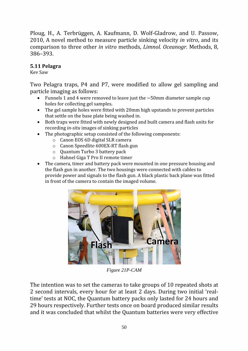
50

Ploug, H., A. Terbrüggen, A. Kaufmann, D. Wolf-Gladrow, and U. Passow, 2010, A novel method to measure particle sinking velocity in vitro, and its comparison to three other in vitro methods, Limnol. Oceanogr. Methods, 8, 386–393. 5.11 Pelagra Kev Saw Two Pelagra traps, P4 and P7, were modified to allow gel sampling and particle imaging as follows:

• Funnels 1 and 4 were removed to leave just the ~50mm diameter sample cup holes for collecting gel samples.

• The gel sample holes were fitted with 20mm high upstands to prevent particles that settle on the base plate being washed in.

• Both traps were fitted with newly designed and built camera and flash units for recording in-situ images of sinking particles

• The photographic setup consisted of the following components: o Canon EOS 6D digital SLR camera o Canon Speedlite 600EX-RT flash gun o Quantum Turbo 3 battery pack o Hahnel Giga T Pro II remote timer

• The camera, timer and battery pack were mounted in one pressure housing and the flash gun in another. The two housings were connected with cables to provide power and signals to the flash gun. A black plastic back plane was fitted in front of the camera to contain the imaged volume.

Figure 21P-CAM

The intention was to set the cameras to take groups of 10 repeated shots at 2 second intervals, every hour for at least 2 days. During two initial ‘real-time’ tests at NOC, the Quantum battery packs only lasted for 24 hours and 29 hours respectively. Further tests once on board produced similar results and it was concluded that whilst the Quantum batteries were very effective

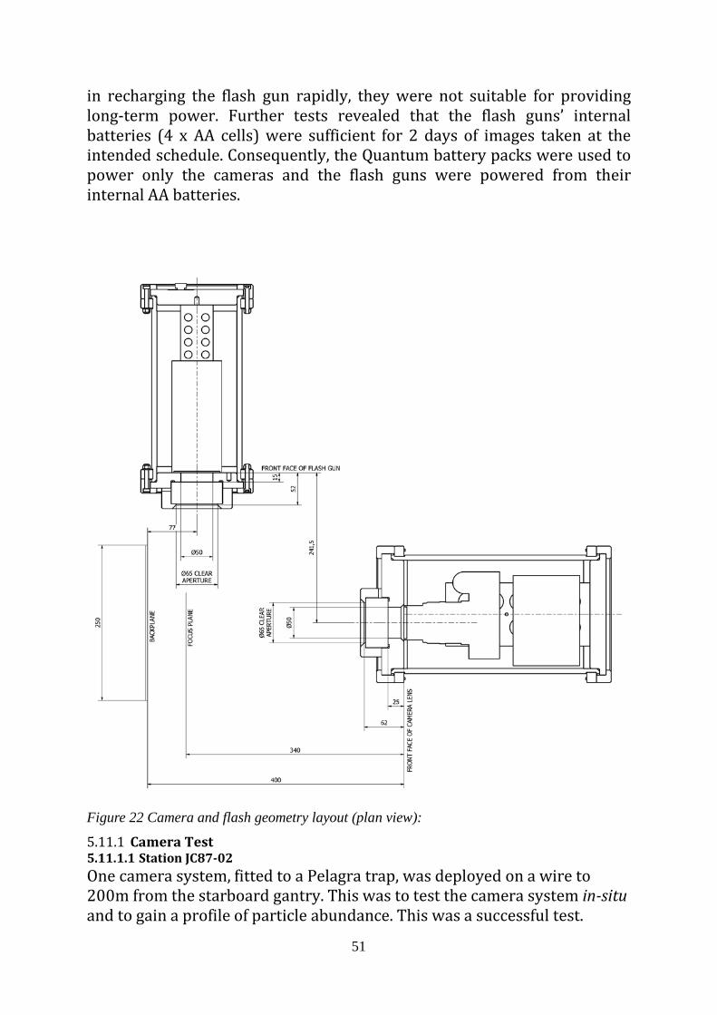
51

in recharging the flash gun rapidly, they were not suitable for providing long-term power. Further tests revealed that the flash guns’ internal batteries (4 x AA cells) were sufficient for 2 days of images taken at the intended schedule. Consequently, the Quantum battery packs were used to power only the cameras and the flash guns were powered from their internal AA batteries.

Figure 22 Camera and flash geometry layout (plan view):

5.11.1 Camera Test 5.11.1.1 Station JC87-02 One camera system, fitted to a Pelagra trap, was deployed on a wire to 200m from the starboard gantry. This was to test the camera system in-situ and to gain a profile of particle abundance. This was a successful test.

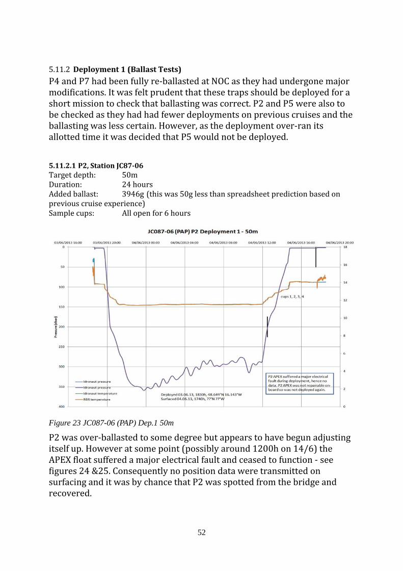
52

5.11.2 Deployment 1 (Ballast Tests) P4 and P7 had been fully re-ballasted at NOC as they had undergone major modifications. It was felt prudent that these traps should be deployed for a short mission to check that ballasting was correct. P2 and P5 were also to be checked as they had had fewer deployments on previous cruises and the ballasting was less certain. However, as the deployment over-ran its allotted time it was decided that P5 would not be deployed. 5.11.2.1 P2, Station JC87-06 Target depth: 50m Duration: 24 hours Added ballast: 3946g (this was 50g less than spreadsheet prediction based on previous cruise experience) Sample cups: All open for 6 hours

Figure 23 JC087-06 (PAP) Dep.1 50m

P2 was over-ballasted to some degree but appears to have begun adjusting itself up. However at some point (possibly around 1200h on 14/6) the APEX float suffered a major electrical fault and ceased to function - see figures 24 &25. Consequently no position data were transmitted on surfacing and it was by chance that P2 was spotted from the bridge and recovered.

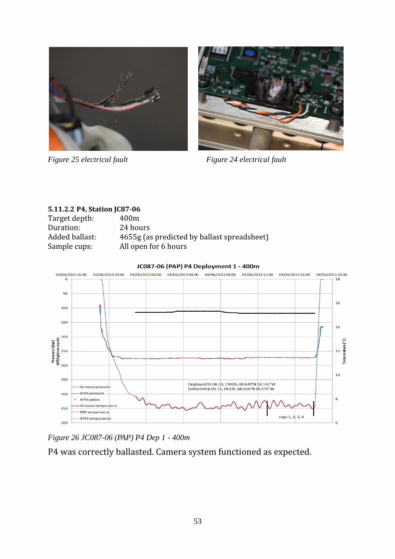
53

Figure 25 electrical fault 5.11.2.2 P4, Station JC87-06 Target depth: 400m Duration: 24 hours Added ballast: 4655g (as predicted by ballast spreadsheet) Sample cups: All open for 6 hours

Figure 26 JC087-06 (PAP) P4 Dep 1 - 400m

P4 was correctly ballasted. Camera system functioned as expected.

Figure 24 electrical fault

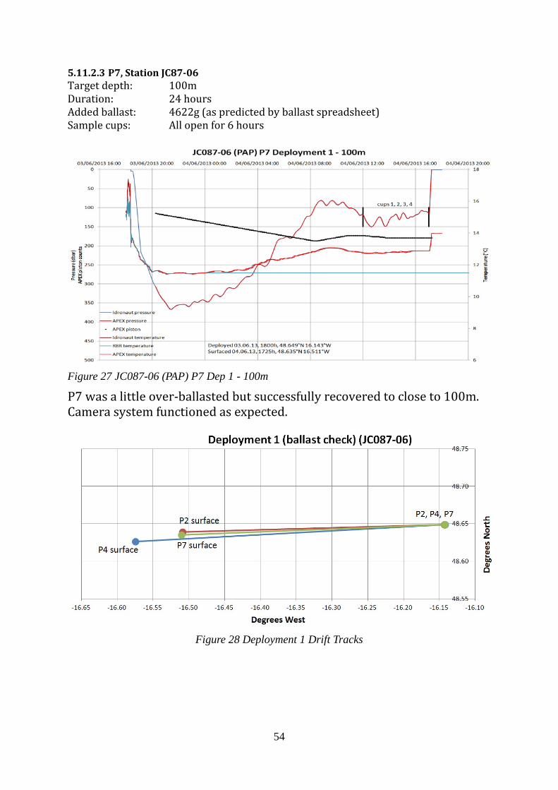
54

5.11.2.3 P7, Station JC87-06 Target depth: 100m Duration: 24 hours Added ballast: 4622g (as predicted by ballast spreadsheet) Sample cups: All open for 6 hours

Figure 27 JC087-06 (PAP) P7 Dep 1 - 100m

P7 was a little over-ballasted but successfully recovered to close to 100m. Camera system functioned as expected.

Figure 28 Deployment 1 Drift Tracks

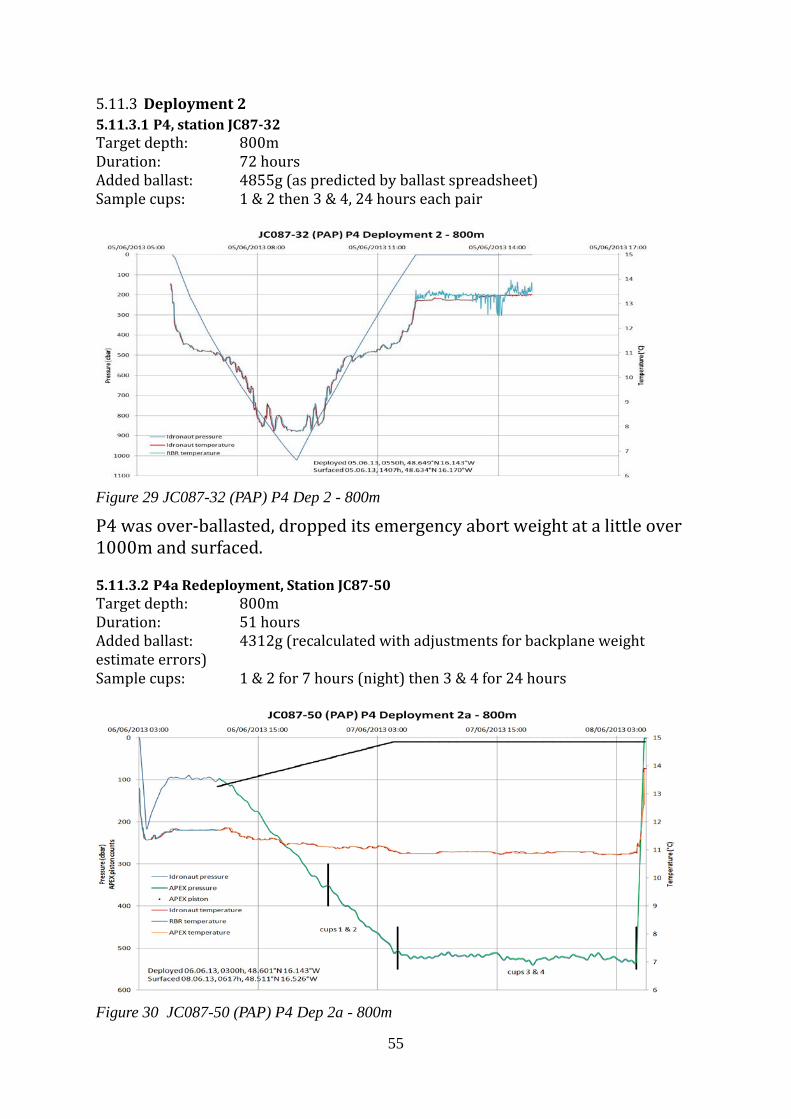
55

5.11.3 Deployment 2 5.11.3.1 P4, station JC87-32 Target depth: 800m Duration: 72 hours Added ballast: 4855g (as predicted by ballast spreadsheet) Sample cups: 1 & 2 then 3 & 4, 24 hours each pair

Figure 29 JC087-32 (PAP) P4 Dep 2 - 800m

P4 was over-ballasted, dropped its emergency abort weight at a little over 1000m and surfaced. 5.11.3.2 P4a Redeployment, Station JC87-50 Target depth: 800m Duration: 51 hours Added ballast: 4312g (recalculated with adjustments for backplane weight estimate errors) Sample cups: 1 & 2 for 7 hours (night) then 3 & 4 for 24 hours

Figure 30 JC087-50 (PAP) P4 Dep 2a - 800m

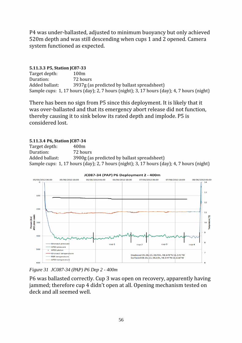
56

P4 was under-ballasted, adjusted to minimum buoyancy but only achieved 520m depth and was still descending when cups 1 and 2 opened. Camera system functioned as expected.

5.11.3.3 P5, Station JC87-33 Target depth: 100m Duration: 72 hours Added ballast: 3937g (as predicted by ballast spreadsheet) Sample cups: 1, 17 hours (day); 2, 7 hours (night); 3, 17 hours (day); 4, 7 hours (night) There has been no sign from P5 since this deployment. It is likely that it was over-ballasted and that its emergency abort release did not function, thereby causing it to sink below its rated depth and implode. P5 is considered lost. 5.11.3.4 P6, Station JC87-34 Target depth: 400m Duration: 72 hours Added ballast: 3900g (as predicted by ballast spreadsheet) Sample cups: 1, 17 hours (day); 2, 7 hours (night); 3, 17 hours (day); 4, 7 hours (night)

Figure 31 JC087-34 (PAP) P6 Dep 2 - 400m

P6 was ballasted correctly. Cup 3 was open on recovery, apparently having jammed; therefore cup 4 didn’t open at all. Opening mechanism tested on deck and all seemed well.

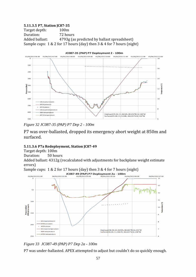
57

5.11.3.5 P7, Station JC87-35 Target depth: 100m Duration: 72 hours Added ballast: 4793g (as predicted by ballast spreadsheet) Sample cups: 1 & 2 for 17 hours (day) then 3 & 4 for 7 hours (night)

Figure 32 JC087-35 (PAP) P7 Dep 2 - 100m

P7 was over-ballasted, dropped its emergency abort weight at 850m and surfaced. 5.11.3.6 P7a Redeployment, Station JC87-49 Target depth: 100m Duration: 50 hours Added ballast: 4312g (recalculated with adjustments for backplane weight estimate errors) Sample cups: 1 & 2 for 17 hours (day) then 3 & 4 for 7 hours (night)

Figure 33 JC087-49 (PAP) P7 Dep 2a - 100m

P7 was under-ballasted. APEX attempted to adjust but couldn’t do so quickly enough.

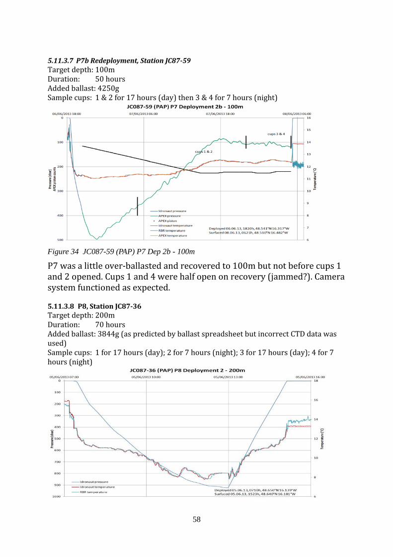
58

5.11.3.7 P7b Redeployment, Station JC87-59 Target depth: 100m Duration: 50 hours Added ballast: 4250g Sample cups: 1 & 2 for 17 hours (day) then 3 & 4 for 7 hours (night)

Figure 34 JC087-59 (PAP) P7 Dep 2b - 100m

P7 was a little over-ballasted and recovered to 100m but not before cups 1 and 2 opened. Cups 1 and 4 were half open on recovery (jammed?). Camera system functioned as expected. 5.11.3.8 P8, Station JC87-36 Target depth: 200m Duration: 70 hours Added ballast: 3844g (as predicted by ballast spreadsheet but incorrect CTD data was used) Sample cups: 1 for 17 hours (day); 2 for 7 hours (night); 3 for 17 hours (day); 4 for 7 hours (night)

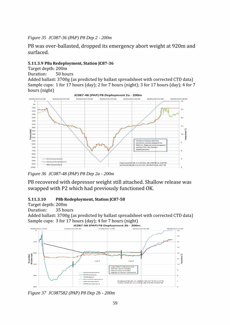
59

Figure 35 JC087-36 (PAP) P8 Dep 2 - 200m

P8 was over-ballasted, dropped its emergency abort weight at 920m and surfaced. 5.11.3.9 P8a Redeployment, Station JC87-36 Target depth: 200m Duration: 50 hours Added ballast: 3700g (as predicted by ballast spreadsheet with corrected CTD data) Sample cups: 1 for 17 hours (day); 2 for 7 hours (night); 3 for 17 hours (day); 4 for 7 hours (night)

Figure 36 JC087-48 (PAP) P8 Dep 2a - 200m

P8 recovered with depressor weight still attached. Shallow release was swapped with P2 which had previously functioned OK. 5.11.3.10 P8b Redeployment, Station JC87-58 Target depth: 200m Duration: 35 hours Added ballast: 3700g (as predicted by ballast spreadsheet with corrected CTD data) Sample cups: 3 for 17 hours (day); 4 for 7 hours (night)

Figure 37 JC087582 (PAP) P8 Dep 2b - 200m

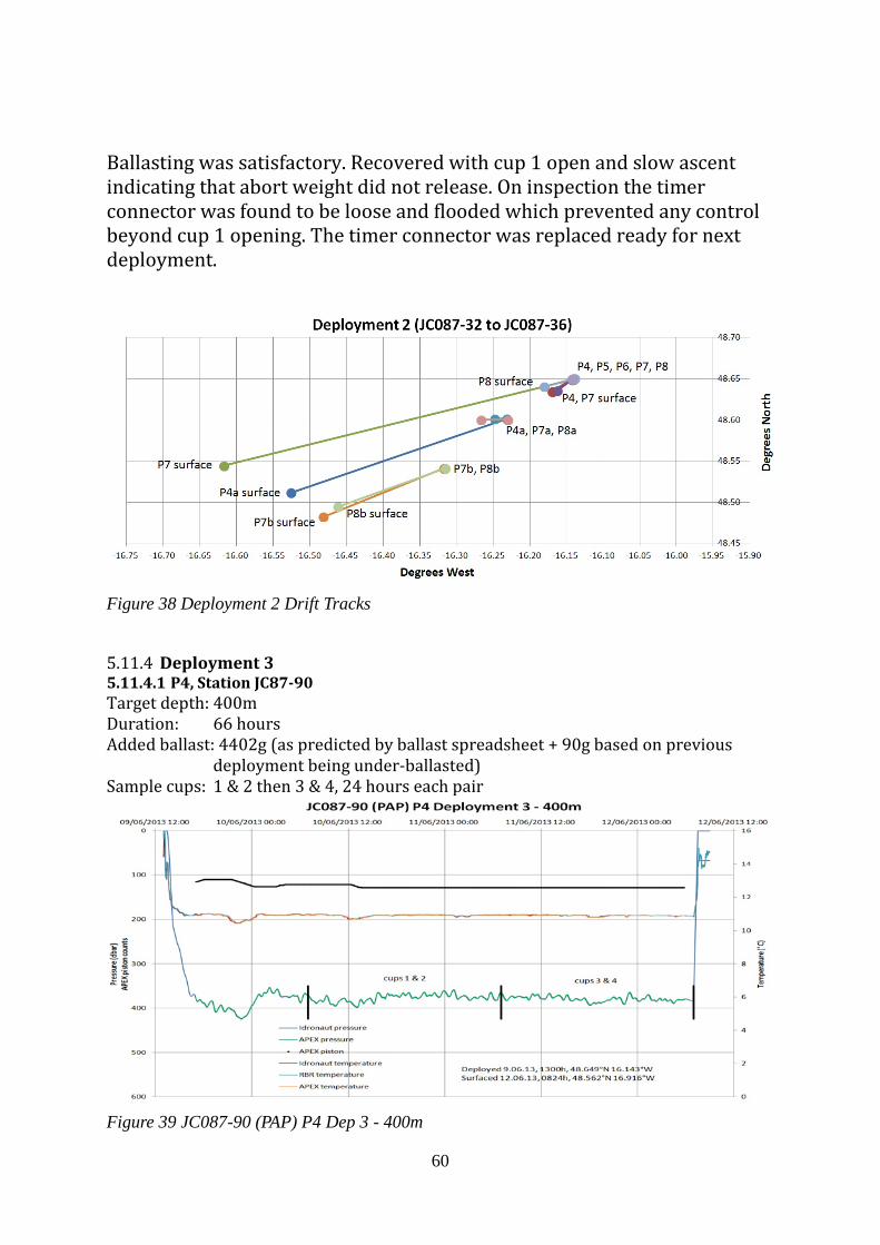
60

Ballasting was satisfactory. Recovered with cup 1 open and slow ascent indicating that abort weight did not release. On inspection the timer connector was found to be loose and flooded which prevented any control beyond cup 1 opening. The timer connector was replaced ready for next deployment.

Figure 38 Deployment 2 Drift Tracks

5.11.4 Deployment 3 5.11.4.1 P4, Station JC87-90 Target depth: 400m Duration: 66 hours Added ballast: 4402g (as predicted by ballast spreadsheet + 90g based on previous

deployment being under-ballasted) Sample cups: 1 & 2 then 3 & 4, 24 hours each pair

Figure 39 JC087-90 (PAP) P4 Dep 3 - 400m

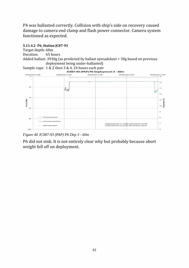
61

P4 was ballasted correctly. Collision with ship’s side on recovery caused damage to camera end clamp and flash power connector. Camera system functioned as expected. 5.11.4.2 P6, Station JC87-93 Target depth: 60m Duration: 65 hours Added ballast: 3930g (as predicted by ballast spreadsheet + 30g based on previous

deployment being under-ballasted) Sample cups: 1 & 2 then 3 & 4, 24 hours each pair

Figure 40 JC087-93 (PAP) P6 Dep 3 - 60m

P6 did not sink. It is not entirely clear why but probably because abort weight fell off on deployment.

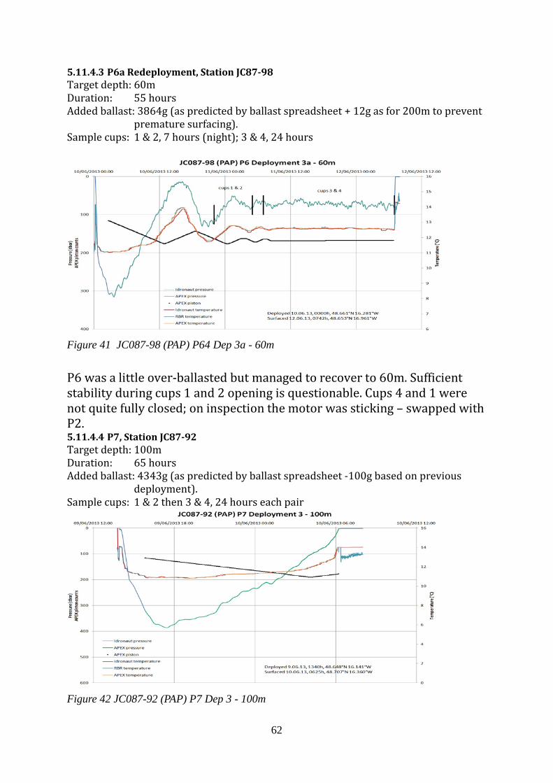
62

5.11.4.3 P6a Redeployment, Station JC87-98 Target depth: 60m Duration: 55 hours Added ballast: 3864g (as predicted by ballast spreadsheet + 12g as for 200m to prevent

premature surfacing). Sample cups: 1 & 2, 7 hours (night); 3 & 4, 24 hours

Figure 41 JC087-98 (PAP) P64 Dep 3a - 60m P6 was a little over-ballasted but managed to recover to 60m. Sufficient stability during cups 1 and 2 opening is questionable. Cups 4 and 1 were not quite fully closed; on inspection the motor was sticking – swapped with P2. 5.11.4.4 P7, Station JC87-92 Target depth: 100m Duration: 65 hours Added ballast: 4343g (as predicted by ballast spreadsheet -100g based on previous

deployment). Sample cups: 1 & 2 then 3 & 4, 24 hours each pair

Figure 42 JC087-92 (PAP) P7 Dep 3 - 100m

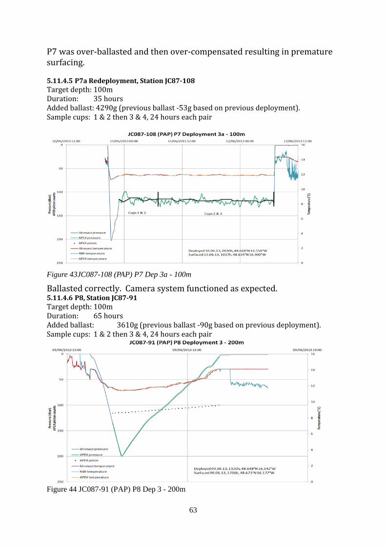
63

P7 was over-ballasted and then over-compensated resulting in premature surfacing. 5.11.4.5 P7a Redeployment, Station JC87-108 Target depth: 100m Duration: 35 hours Added ballast: 4290g (previous ballast -53g based on previous deployment). Sample cups: 1 & 2 then 3 & 4, 24 hours each pair

Figure 43JC087-108 (PAP) P7 Dep 3a - 100m

Ballasted correctly. Camera system functioned as expected. 5.11.4.6 P8, Station JC87-91 Target depth: 100m Duration: 65 hours Added ballast: 3610g (previous ballast -90g based on previous deployment). Sample cups: 1 & 2 then 3 & 4, 24 hours each pair

Figure 44 JC087-91 (PAP) P8 Dep 3 - 200m

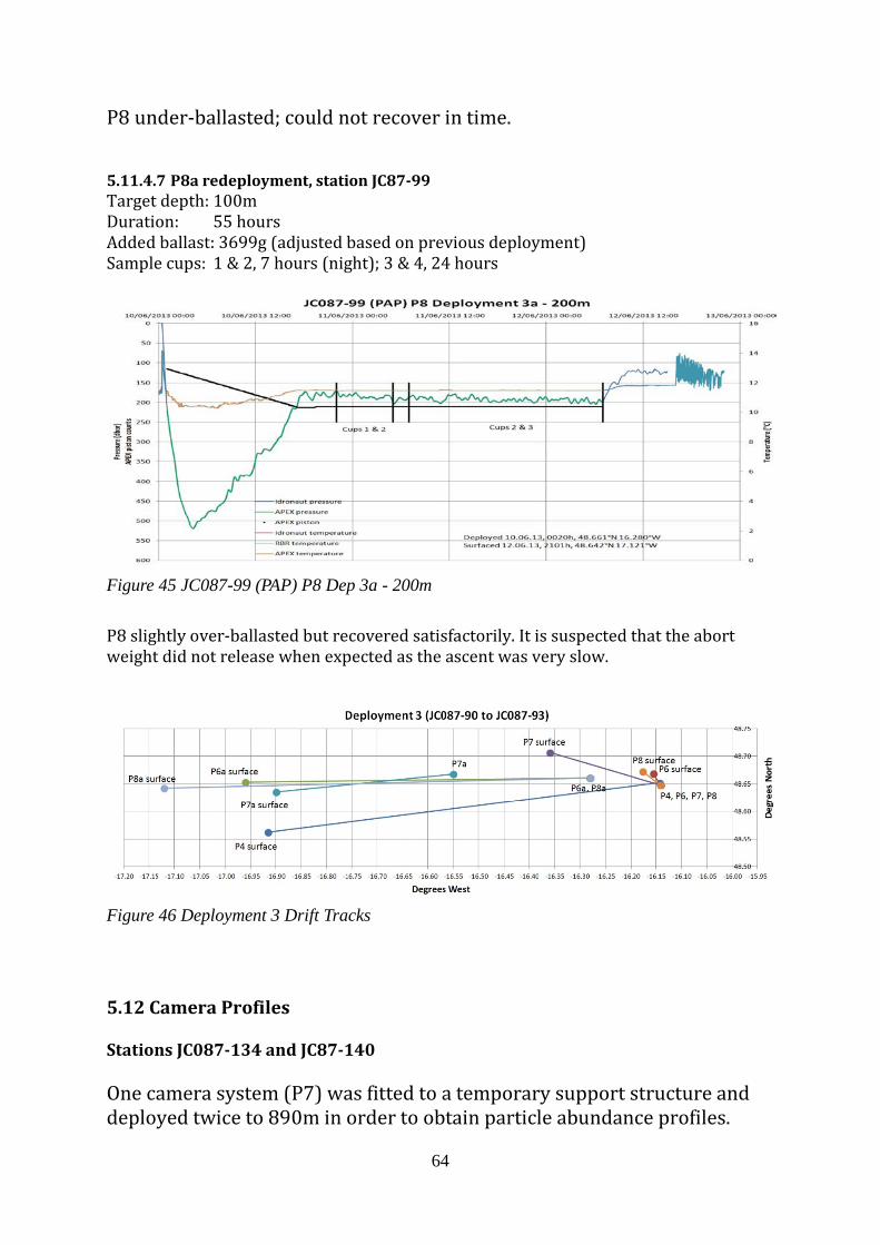
64

P8 under-ballasted; could not recover in time. 5.11.4.7 P8a redeployment, station JC87-99 Target depth: 100m Duration: 55 hours Added ballast: 3699g (adjusted based on previous deployment) Sample cups: 1 & 2, 7 hours (night); 3 & 4, 24 hours

Figure 45 JC087-99 (PAP) P8 Dep 3a - 200m P8 slightly over-ballasted but recovered satisfactorily. It is suspected that the abort weight did not release when expected as the ascent was very slow.

Figure 46 Deployment 3 Drift Tracks 5.12 Camera Profiles Stations JC087-134 and JC87-140 One camera system (P7) was fitted to a temporary support structure and deployed twice to 890m in order to obtain particle abundance profiles.

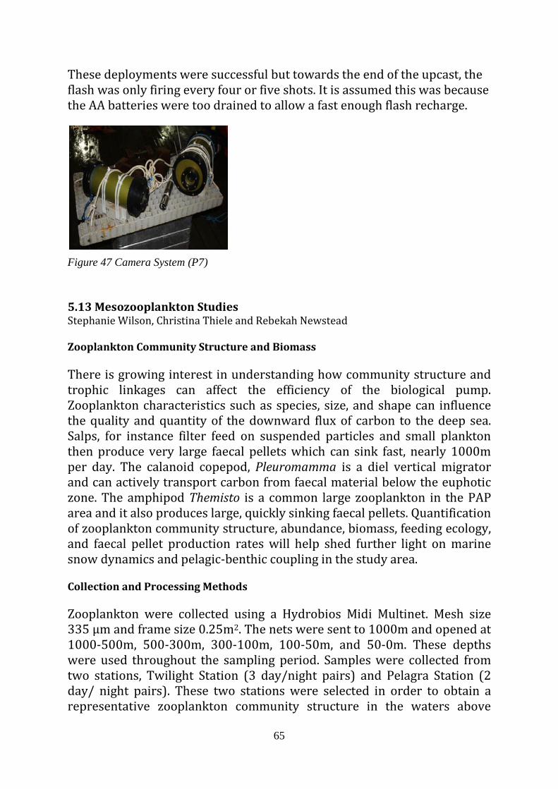
65

These deployments were successful but towards the end of the upcast, the flash was only firing every four or five shots. It is assumed this was because the AA batteries were too drained to allow a fast enough flash recharge.

Figure 47 Camera System (P7) 5.13 Mesozooplankton Studies Stephanie Wilson, Christina Thiele and Rebekah Newstead Zooplankton Community Structure and Biomass There is growing interest in understanding how community structure and trophic linkages can affect the efficiency of the biological pump. Zooplankton characteristics such as species, size, and shape can influence the quality and quantity of the downward flux of carbon to the deep sea. Salps, for instance filter feed on suspended particles and small plankton then produce very large faecal pellets which can sink fast, nearly 1000m per day. The calanoid copepod, Pleuromamma is a diel vertical migrator and can actively transport carbon from faecal material below the euphotic zone. The amphipod Themisto is a common large zooplankton in the PAP area and it also produces large, quickly sinking faecal pellets. Quantification of zooplankton community structure, abundance, biomass, feeding ecology, and faecal pellet production rates will help shed further light on marine snow dynamics and pelagic-benthic coupling in the study area. Collection and Processing Methods

Zooplankton were collected using a Hydrobios Midi Multinet. Mesh size 335 µm and frame size 0.25m2. The nets were sent to 1000m and opened at 1000-500m, 500-300m, 300-100m, 100-50m, and 50-0m. These depths were used throughout the sampling period. Samples were collected from two stations, Twilight Station (3 day/night pairs) and Pelagra Station (2 day/ night pairs). These two stations were selected in order to obtain a representative zooplankton community structure in the waters above

66

where the Pelagra sediment traps were deployed (Twilight) and predicted to recover (Pelagra). Zooplankton were processed for biomass, abundance and community structure, grazing impact, and to determine gut contents using DNA-based molecular techniques. Upon Multinet retrieval the nets were rinsed into the cod-end containers and the samples poured into 5L buckets. These were mixed with 10% soda water to anesthetize the zooplankton to avoid bucket feeding and egestion. Until splitting, the samples were kept in the dark in a cold room set to the temperature of the mixed layer depth (13oC). One at a time, starting from the shallowest depth, the samples were split into 4-8 parts. 1/2 of the sample was processed for biomass (see below), 1/4 of the sample was preserved in 4% buffered formalin for abundance and community structure estimates, and 1/4 to 1/8 of the sample was set aside and frozen at -80oC for analyses of grazing impact and DNA extraction back at Bangor University. The biomass split was poured directly into a set of 5 nested sieves. 200, 500, 1000, 2000, and 5000µm to size fractionate the sample. Once separated the fractions were placed onto preweighed 200 µm nitex circles and into petri dishes. These were stored at -80oC until further laboratory processing for wet and dry weights. Chlorophyll a was measured from the deep CTD cast to 4700m at several depths coinciding with multinet depths (0-1000m). This was completed as it is required in the calculations to measure grazing impact.

Faecal Pellet Production Rate, Egestion and Excretion Rate Methods

There were three experiments throughout the cruise to determine faecal pellet production, egestion, and excretion rates (FP1-3). A marine snow catcher device was used to collect seawater for faecal pellet production rate incubations 1-2 hrs before the zooplankton net tows for live animals. These devices were sent to the depth of the chlorophyll maximum (45-55m). When on the surface, water was gently filtered through a silicon tube with a 200µm mesh attached to exclude microzooplankton but include small plankton for grazing. 0.2µm filtered seawater was used for the egestion and excretion experiments. Live zooplankton were collected using a 0.25m diameter WP2 ring net with 50µm mesh. A series of WP2 tows were conducted at night to collect vertical migrators which will be likely contributing the most to active and passive carbon flux out of the euphotic zone. Zooplankton selected for

67

incubation included Salpa sp. Salps, Pleuromamma sp. calanoid copepods, and Themisto sp. amphipods. These were the most common of the larger species of zooplankton collected in the nets. Salps were immediately removed from the bucket and gently rinsed several times in 200µm filtered seawater was used for the egestion and excretion experiments. Filtered seawater. Salps in excellent condition were selected for incubations. One salp was placed in each of 5 1L straight sided plastic jars and incubated for 6 hrs in the cold room set to near MLD temperature. Pleuromamma copepods were gently picked out of the net haul using wide pipettes and placed in 200µm filtered seawater to rinse before the experiments. Five animals for each incubation chamber were again gently separated and placed in new 200µm filtered seawater in multi-welled plates for a second rinse and then put into faecal pellet collection trap incubation jars which separate the animal from their faecal pellets to avoid coprophagy (poop traps). The copepods were incubated in 200µm filtered seawater for 6-8hrs. Themisto amphipods were treated in a similar fashion to the Pleuromamma copepods (n=3 or 12 per jar) and incubated 6-9 hrs. Upon completion of the incubations, zooplankton were removed and preserved in 4% buffered formalin and the faecal pellets were collected, counted, and photographed. The faecal pellets were then placed in a 2ml cryovial and frozen at -80oC for later molecular analysis for prey type. A subset of Pleuromamma copepods were also incubated in 1L 0.2um filtered seawater to measure egestion and excretion rates. N=5, FP1,2,3. Aliquots of the seawater before and after the incubations were processed for nutrients onboard the RRS James Cook. These experiments were otherwise similar in procedure to the faecal pellet production rate experiments. Post-cruise Frozen biomass samples will be thawed in the lab for 20 minutes, wet-weighed then placed in a drying oven at 50oC overnight and dry-weighed. Zooplankton in the 4% buffered formalin preserved samples will be sorted and classified into major groups with the major calanoid copepods identified to species level if possible. This data will be used in Christina Thiele’s master thesis. Samples set aside for grazing impact will be processed for gut chlorophyll by Rebekah Newstead and an undergraduate volunteer. Samples set aside

68

for DNA analysis will be stored in a -80oC until funding can be secured to use next generation sequencing using an Illumnia sequencer. Predicted Outputs There is the potential for at least three manuscripts from this cruise. Christina Thiele will produce a Masters thesis and manuscript using data collected for biomass and community structure. Rebekah Newstead will produce a manuscript on grazing impact and likely use this as a chapter in her PhD dissertation. The data collected for faecal pellet production, egestion, and excretion can be used in a collaborative manuscript with Morten Iverson and Richard Lampitt using data from the Pelagra traps on the contribution of zooplankton to particle export in the region. The data generated from this project can also be used in collaboration with Marja Koski and Frederica Norrbin.

5.14 Underway Sampling Antony Birchill, Oliver Willmot, Gillian Damerell, Zoe Morrall, Anna Rumyantseva, Anna Belcher, Adrian Martin and Gayatri Dudeja Objective To take regular samples of the ships non-toxic underway supply to provide a time series of chlorophyll, salinity and nutrient data. These data will be used to calibrate underway instrument data after our return to NOC. Methods Samples from the ships underway (5m depth) for chlorophyll, salinity and nutrient analysis were taken approximately every 4 hours from 0800 (GMT) on 03/06/2013 (J154) to 1200 (GMT) on 15/06/2013 (J166). All sampling bottles were rinsed 3 times with sample water prior to sample collection. Chlorophyll 250ml of sample water was collected in a dark bottle and filtered through 25mm GF/F Whatman filters. Filter then stored in a glass vial with 8ml of acetone and kept in a refrigerator for 18-20 hours before on board fluorescence analysis. Nutrients Two samples were collected for nutrient analysis in 15ml centrifuge tubes, a 10ml sample frozen for later analysis and a 14ml sample for onboard analysis.

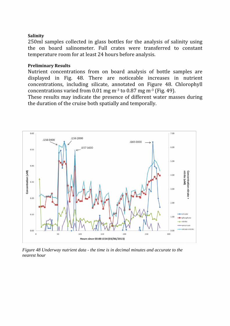
69

Salinity 250ml samples collected in glass bottles for the analysis of salinity using the on board salinometer. Full crates were transferred to constant temperature room for at least 24 hours before analysis. Preliminary Results Nutrient concentrations from on board analysis of bottle samples are displayed in Fig. 48. There are noticeable increases in nutrient concentrations, including silicate, annotated on Figure 48. Chlorophyll concentrations varied from 0.01 mg m-3 to 0.87 mg m-3 (Fig. 49). These results may indicate the presence of different water masses during the duration of the cruise both spatially and temporally.

Fig. 26 Underway nutrient data - the time is in decimal minutes and accurate to the nearest 5 minutes

Figure 48 Underway nutrient data - the time is in decimal minutes and accurate to the nearest hour

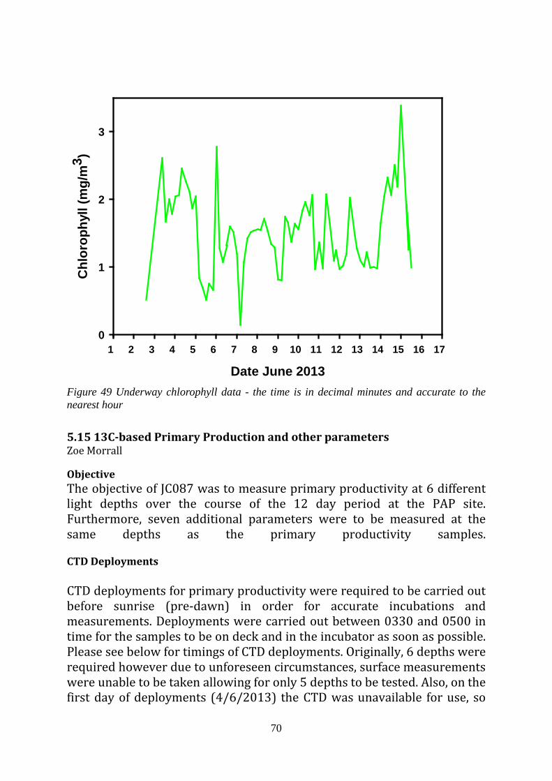
70

Figure 49 Underway chlorophyll data - the time is in decimal minutes and accurate to the nearest hour 5.15 13C-based Primary Production and other parameters Zoe Morrall Objective The objective of JC087 was to measure primary productivity at 6 different light depths over the course of the 12 day period at the PAP site. Furthermore, seven additional parameters were to be measured at the same depths as the primary productivity samples. CTD Deployments CTD deployments for primary productivity were required to be carried out before sunrise (pre-dawn) in order for accurate incubations and measurements. Deployments were carried out between 0330 and 0500 in time for the samples to be on deck and in the incubator as soon as possible. Please see below for timings of CTD deployments. Originally, 6 depths were required however due to unforeseen circumstances, surface measurements were unable to be taken allowing for only 5 depths to be tested. Also, on the first day of deployments (4/6/2013) the CTD was unavailable for use, so

Date June 2013

1 2 3 4 5 6 7 8 9 10 11 12 13 14 15 16 17

Chl

orop

hyll

(mg/

m3 )

0

1

2

3

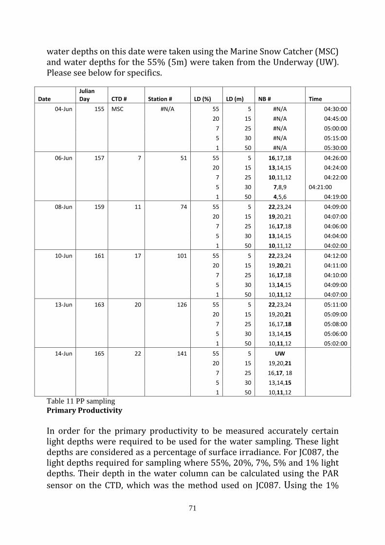
71

water depths on this date were taken using the Marine Snow Catcher (MSC) and water depths for the 55% (5m) were taken from the Underway (UW). Please see below for specifics.

Date Julian Day CTD # Station # LD (%) LD (m) NB # Time

04-Jun 155 MSC #N/A 55 5 #N/A 04:30:00 20 15 #N/A 04:45:00 7 25 #N/A 05:00:00 5 30 #N/A 05:15:00 1 50 #N/A 05:30:00

06-Jun 157 7 51 55 5 16,17,18 04:26:00 20 15 13,14,15 04:24:00 7 25 10,11,12 04:22:00 5 30 7,8,9 04:21:00 1 50 4,5,6 04:19:00

08-Jun 159 11 74 55 5 22,23,24 04:09:00 20 15 19,20,21 04:07:00 7 25 16,17,18 04:06:00 5 30 13,14,15 04:04:00 1 50 10,11,12 04:02:00

10-Jun 161 17 101 55 5 22,23,24 04:12:00 20 15 19,20,21 04:11:00 7 25 16,17,18 04:10:00 5 30 13,14,15 04:09:00 1 50 10,11,12 04:07:00

13-Jun 163 20 126 55 5 22,23,24 05:11:00 20 15 19,20,21 05:09:00 7 25 16,17,18 05:08:00 5 30 13,14,15 05:06:00 1 50 10,11,12 05:02:00

14-Jun 165 22 141 55 5 UW 20 15 19,20,21

7 25 16,17, 18 5 30 13,14,15 1 50 10,11,12

Table 11 PP sampling Primary Productivity In order for the primary productivity to be measured accurately certain light depths were required to be used for the water sampling. These light depths are considered as a percentage of surface irradiance. For JC087, the light depths required for sampling where 55%, 20%, 7%, 5% and 1% light depths. Their depth in the water column can be calculated using the PAR sensor on the CTD, which was the method used on JC087. Using the 1%

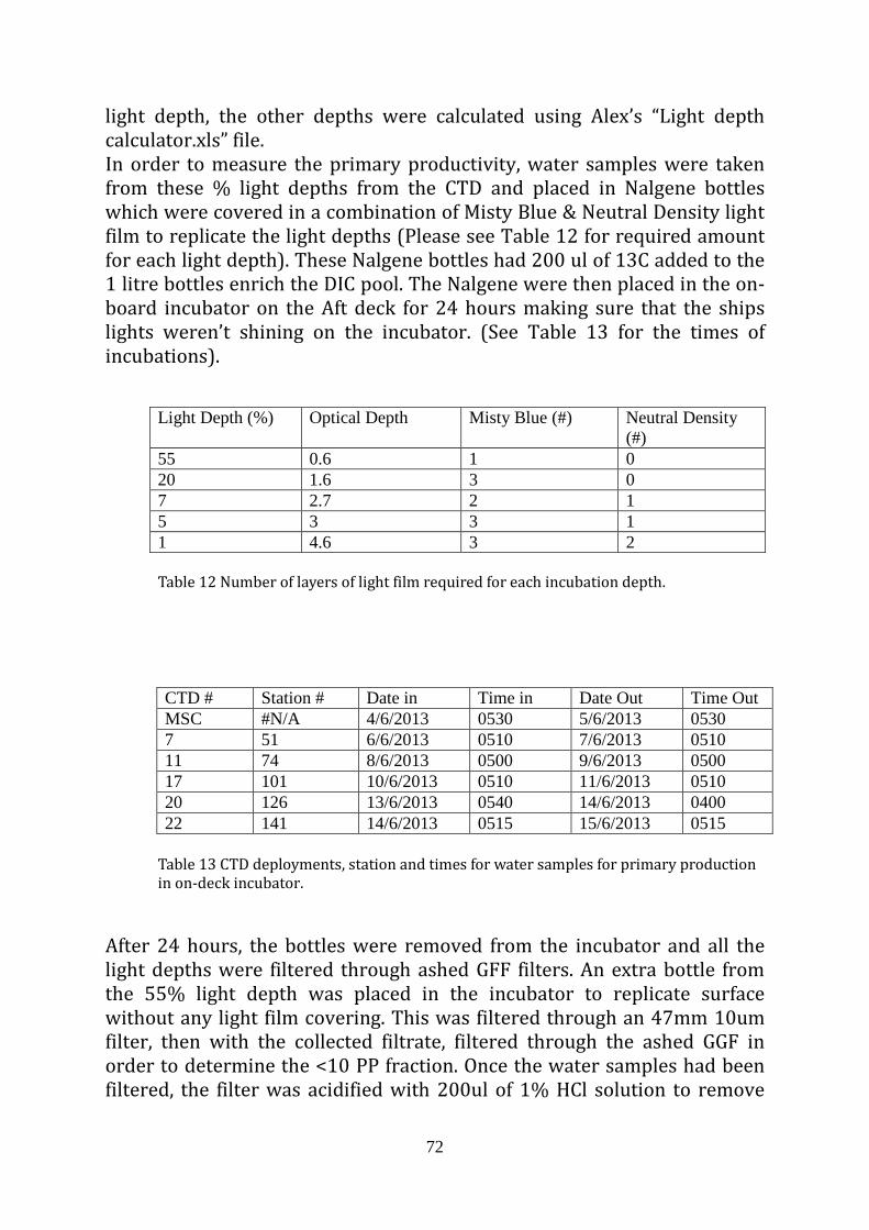
72

light depth, the other depths were calculated using Alex’s “Light depth calculator.xls” file. In order to measure the primary productivity, water samples were taken from these % light depths from the CTD and placed in Nalgene bottles which were covered in a combination of Misty Blue & Neutral Density light film to replicate the light depths (Please see Table 12 for required amount for each light depth). These Nalgene bottles had 200 ul of 13C added to the 1 litre bottles enrich the DIC pool. The Nalgene were then placed in the on-board incubator on the Aft deck for 24 hours making sure that the ships lights weren’t shining on the incubator. (See Table 13 for the times of incubations).

Light Depth (%) Optical Depth Misty Blue (#) Neutral Density

(#) 55 0.6 1 0 20 1.6 3 0 7 2.7 2 1 5 3 3 1 1 4.6 3 2 Table 12 Number of layers of light film required for each incubation depth.

CTD # Station # Date in Time in Date Out Time Out MSC #N/A 4/6/2013 0530 5/6/2013 0530 7 51 6/6/2013 0510 7/6/2013 0510 11 74 8/6/2013 0500 9/6/2013 0500 17 101 10/6/2013 0510 11/6/2013 0510 20 126 13/6/2013 0540 14/6/2013 0400 22 141 14/6/2013 0515 15/6/2013 0515

Table 13 CTD deployments, station and times for water samples for primary production in on-deck incubator.

After 24 hours, the bottles were removed from the incubator and all the light depths were filtered through ashed GFF filters. An extra bottle from the 55% light depth was placed in the incubator to replicate surface without any light film covering. This was filtered through an 47mm 10um filter, then with the collected filtrate, filtered through the ashed GGF in order to determine the <10 PP fraction. Once the water samples had been filtered, the filter was acidified with 200ul of 1% HCl solution to remove

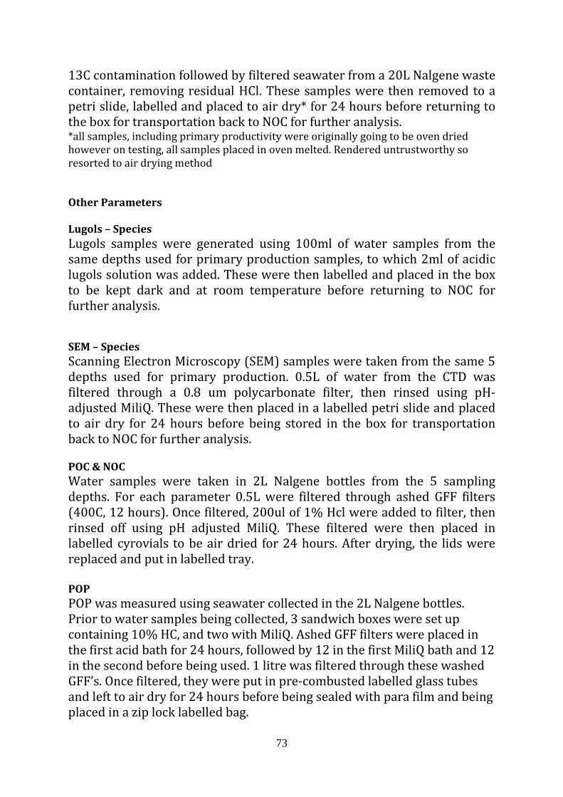
73

13C contamination followed by filtered seawater from a 20L Nalgene waste container, removing residual HCl. These samples were then removed to a petri slide, labelled and placed to air dry* for 24 hours before returning to the box for transportation back to NOC for further analysis. *all samples, including primary productivity were originally going to be oven dried however on testing, all samples placed in oven melted. Rendered untrustworthy so resorted to air drying method Other Parameters Lugols – Species Lugols samples were generated using 100ml of water samples from the same depths used for primary production samples, to which 2ml of acidic lugols solution was added. These were then labelled and placed in the box to be kept dark and at room temperature before returning to NOC for further analysis. SEM – Species Scanning Electron Microscopy (SEM) samples were taken from the same 5 depths used for primary production. 0.5L of water from the CTD was filtered through a 0.8 um polycarbonate filter, then rinsed using pH-adjusted MiliQ. These were then placed in a labelled petri slide and placed to air dry for 24 hours before being stored in the box for transportation back to NOC for further analysis. POC & NOC Water samples were taken in 2L Nalgene bottles from the 5 sampling depths. For each parameter 0.5L were filtered through ashed GFF filters (400C, 12 hours). Once filtered, 200ul of 1% Hcl were added to filter, then rinsed off using pH adjusted MiliQ. These filtered were then placed in labelled cyrovials to be air dried for 24 hours. After drying, the lids were replaced and put in labelled tray. POP POP was measured using seawater collected in the 2L Nalgene bottles. Prior to water samples being collected, 3 sandwich boxes were set up containing 10% HC, and two with MiliQ. Ashed GFF filters were placed in the first acid bath for 24 hours, followed by 12 in the first MiliQ bath and 12 in the second before being used. 1 litre was filtered through these washed GFF’s. Once filtered, they were put in pre-combusted labelled glass tubes and left to air dry for 24 hours before being sealed with para film and being placed in a zip lock labelled bag.

74

BSi & PIC Seawater was collected from the same sampling depths determined by the back calculated depths. For both BSi and PIC 0.5L were filtered through a 0.8um polycarbonate filter, then rinsed with pH-adjusted MiliQ and placed in a labelled Falcon tube to be air dried for 24 hours before being placed in a zip lock bag. Further Work On returning to NOC, all samples will be processed in order to compile a full data set of measurements taken on board JC087 for the 6 depths measured over 6 pre-dawn CTD’s. 5.16 Turbulence Measurements Anna Rumyantseva, Adrian Martin and Gillian Damarell Summary of Turbulence Stations From experience of analyzing turbulence probe data from the previous cruises to the PAP site it was decided that on every station profiling time would be at least 2 hours (~ 12 profiles per station). This is because the above analysis revealed the turbulent diffusivities to be log-normally distributed (if not worse) with the causative mixing being intermittent. Therefore approximately 10 is viewed as the smallest practical number of profiles to calculate robust profiles of mean turbulent diffusivity. The turbulence probe was also equipped with a fluorescence sensor. In the beginning of the cruise we did not have proper software to obtain data from the chlorophyll channel. Therefore the first 3 stations do not have fluorescence data. Later we sent an email to Sun & Sea Technology and a new, correct version of the probe file needed by the software was provided. The turbulence stations were conducted at the “Twilight station” located at 48o 38.9N 16o 08.5W in the south-east of the OSMOSIS array. OSMOSIS Seagliders deployed at the sampling site showed significant increase in chlorophyll concentration at the beginning of the JC087 cruise. We hope that our measurements captured detailed evolution of a water column and chlorophyll distribution during this important event in a phytoplankton annual cycle. Before or/and after every turbulence station a CTD profile was obtained to collect water samples for phytoplankton species composition and nutrients analysis. The list of CTD stations related to turbulence stations is summarized in the Table 13. In addition to hopefully providing an excellent dataset, the cruise was also useful in training personnel in use of the new equipment. The laptop end of

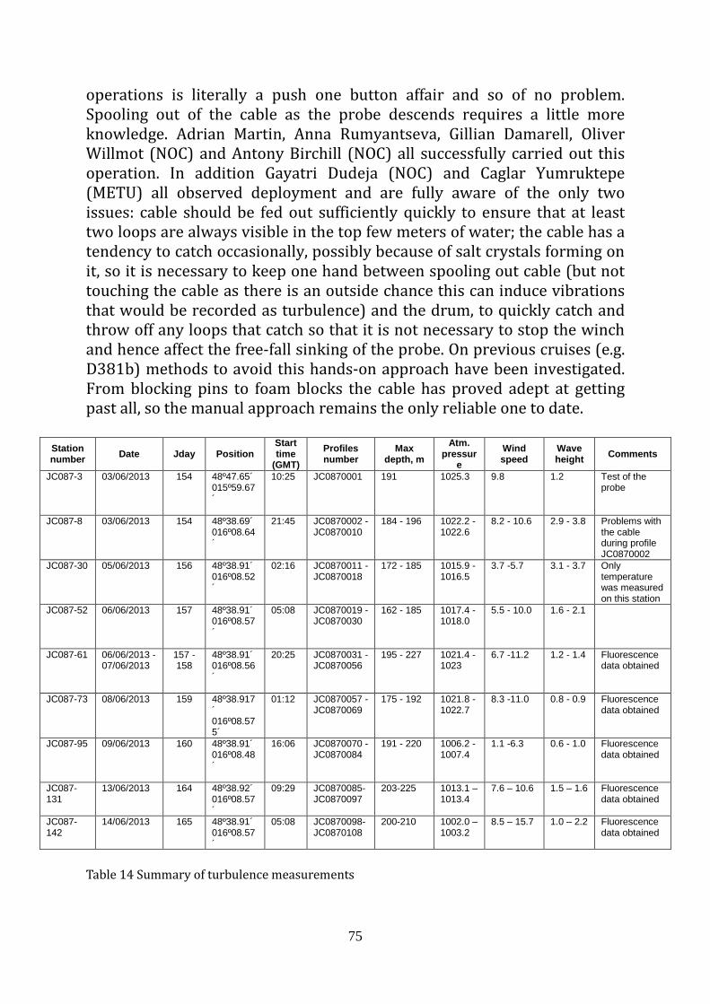
75

operations is literally a push one button affair and so of no problem. Spooling out of the cable as the probe descends requires a little more knowledge. Adrian Martin, Anna Rumyantseva, Gillian Damarell, Oliver Willmot (NOC) and Antony Birchill (NOC) all successfully carried out this operation. In addition Gayatri Dudeja (NOC) and Caglar Yumruktepe (METU) all observed deployment and are fully aware of the only two issues: cable should be fed out sufficiently quickly to ensure that at least two loops are always visible in the top few meters of water; the cable has a tendency to catch occasionally, possibly because of salt crystals forming on it, so it is necessary to keep one hand between spooling out cable (but not touching the cable as there is an outside chance this can induce vibrations that would be recorded as turbulence) and the drum, to quickly catch and throw off any loops that catch so that it is not necessary to stop the winch and hence affect the free-fall sinking of the probe. On previous cruises (e.g. D381b) methods to avoid this hands-on approach have been investigated. From blocking pins to foam blocks the cable has proved adept at getting past all, so the manual approach remains the only reliable one to date.

Station number Date Jday Position

Start time

(GMT) Profiles number

Max depth, m

Atm. pressur

e Wind speed

Wave height Comments

JC087-3 03/06/2013

154 48º47.65´ 015º59.67´

10:25 JC0870001 191 1025.3 9.8 1.2 Test of the probe

JC087-8 03/06/2013 154 48º38.69´ 016º08.64´

21:45 JC0870002 - JC0870010

184 - 196 1022.2 - 1022.6

8.2 - 10.6 2.9 - 3.8 Problems with the cable during profile JC0870002

JC087-30 05/06/2013

156 48º38.91´ 016º08.52´

02:16 JC0870011 - JC0870018

172 - 185 1015.9 - 1016.5

3.7 -5.7 3.1 - 3.7 Only temperature was measured on this station

JC087-52 06/06/2013 157 48º38.91´ 016º08.57´

05:08 JC0870019 - JC0870030

162 - 185 1017.4 - 1018.0

5.5 - 10.0 1.6 - 2.1

JC087-61 06/06/2013 -07/06/2013

157 - 158

48º38.91´ 016º08.56´

20:25 JC0870031 - JC0870056

195 - 227 1021.4 - 1023

6.7 -11.2 1.2 - 1.4 Fluorescence data obtained

JC087-73 08/06/2013

159 48º38.917´ 016º08.575´

01:12 JC0870057 - JC0870069

175 - 192 1021.8 - 1022.7

8.3 -11.0 0.8 - 0.9 Fluorescence data obtained

JC087-95 09/06/2013

160 48º38.91´ 016º08.48´

16:06 JC0870070 - JC0870084

191 - 220 1006.2 - 1007.4

1.1 -6.3 0.6 - 1.0 Fluorescence data obtained

JC087-131

13/06/2013 164 48º38.92´ 016º08.57´

09:29 JC0870085-JC0870097

203-225 1013.1 – 1013.4

7.6 – 10.6 1.5 – 1.6 Fluorescence data obtained

JC087-142

14/06/2013 165 48º38.91´ 016º08.57´

05:08 JC0870098-JC0870108

200-210 1002.0 – 1003.2

8.5 – 15.7 1.0 – 2.2 Fluorescence data obtained

Table 14 Summary of turbulence measurements

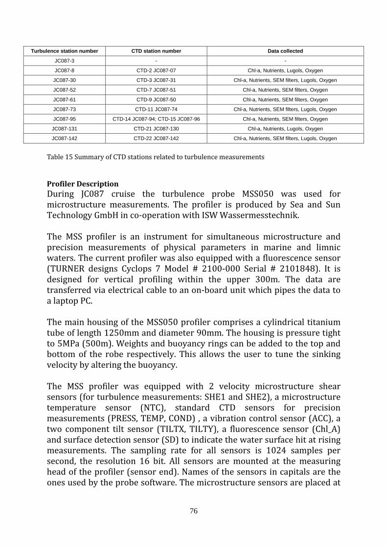
76

Turbulence station number CTD station number Data collected

JC087-3 - -

JC087-8 CTD-2 JC087-07 Chl-a, Nutrients, Lugols, Oxygen

JC087-30 CTD-3 JC087-31 Chl-a, Nutrients, SEM filters, Lugols, Oxygen

JC087-52 CTD-7 JC087-51 Chl-a, Nutrients, SEM filters, Oxygen

JC087-61 CTD-9 JC087-50 Chl-a, Nutrients, SEM filters, Oxygen

JC087-73 CTD-11 JC087-74 Chl-a, Nutrients, SEM filters, Lugols, Oxygen

JC087-95 CTD-14 JC087-94; CTD-15 JC087-96 Chl-a, Nutrients, SEM filters, Oxygen

JC087-131 CTD-21 JC087-130 Chl-a, Nutrients, Lugols, Oxygen

JC087-142 CTD-22 JC087-142 Chl-a, Nutrients, SEM filters, Lugols, Oxygen

Table 15 Summary of CTD stations related to turbulence measurements Profiler Description During JC087 cruise the turbulence probe MSS050 was used for microstructure measurements. The profiler is produced by Sea and Sun Technology GmbH in co-operation with ISW Wassermesstechnik. The MSS profiler is an instrument for simultaneous microstructure and precision measurements of physical parameters in marine and limnic waters. The current profiler was also equipped with a fluorescence sensor (TURNER designs Cyclops 7 Model # 2100-000 Serial # 2101848). It is designed for vertical profiling within the upper 300m. The data are transferred via electrical cable to an on-board unit which pipes the data to a laptop PC. The main housing of the MSS050 profiler comprises a cylindrical titanium tube of length 1250mm and diameter 90mm. The housing is pressure tight to 5MPa (500m). Weights and buoyancy rings can be added to the top and bottom of the robe respectively. This allows the user to tune the sinking velocity by altering the buoyancy. The MSS profiler was equipped with 2 velocity microstructure shear sensors (for turbulence measurements: SHE1 and SHE2), a microstructure temperature sensor (NTC), standard CTD sensors for precision measurements (PRESS, TEMP, COND) , a vibration control sensor (ACC), a two component tilt sensor (TILTX, TILTY), a fluorescence sensor (Chl_A) and surface detection sensor (SD) to indicate the water surface hit at rising measurements. The sampling rate for all sensors is 1024 samples per second, the resolution 16 bit. All sensors are mounted at the measuring head of the profiler (sensor end). Names of the sensors in capitals are the ones used by the probe software. The microstructure sensors are placed at

77

the tip of a slim shaft, about 150mm in front of the CTD sensors to ensure that they are not affected by passage of others through water. The general behaviour of the MSS profiler is described in detail by Prandke, Holtsch and Stips (2000). Background to Microstructure Shear Measurement For measurements of velocity microstructure (turbulence), the MSS profiler is equipped with two shear probes PNS01 (serial # 98 and # 99). This type of shear probe comprises an axially symmetric airfoil separated by a cantilever from a piezoelectric beam. The piezoelectric bending element is isolated by a Teflon tube from water. This gives the sensor excellent long-term stability. The length and diameter of the airfoil are 4mm and 3mm respectively. The spatial resolution of the PNS shear probe is approx 8mm. The general behavior of an airfoil sensor has been described in detail by Osborn and Crawford (1980). The mean velocity due to the profiling speed of the probe is aligned with the axis of revolution. While the probe is not sensitive to axial forces, the cross-stream (transverse) components of turbulent velocity produce a lifting force at the airfoil. The piezoelectric beam senses the lift force. The output of the piezoelectric element is a voltage proportional to the instantaneous cross-stream component of the velocity field. Deployment and Operation of the Microstructure Measuring System The MSS was operated via a winch ISW SWM1000, mounted on the port stern quarter of the vessel. During the MSS measurements, two methods were used for positioning the ship to avoid the cable catching in a propeller. The method previously used is to have the ship was moving with speed approx. 0.5-1.0 knots with respect to the water against the wind. An alternative, devised by the Chief Officer and more commonly used on JC87 was to hold the ship geographically stationary with port propeller off such that cable streamed with current to aft/port. Amore generally it is also important to note that azimuth pod thruster must be off to avoid generating turbulence below the ship’s depth. Disturbing effects caused by cable tension (vibrations) and the ship’s movement were minimized by maintaining slack in the cable at descent – as a rule of thumb two “loops” should always be visible just below the sea surface. In order to take into account the intermittent nature of marine turbulence, repeated MSS measurements were carried out in bursts of typically 10 profiles per station. The measurement interval was approx. 10/9 min for a profile to 170/150dbar. The profiler fell to a depth of typically 170-200dbar even though the winch was stopped when the pressure reached

78

160/140dbar. The excess 30-40dbar in depth was due to the amount of slack in the cable. As the profiler is rated to 300m it was felt that the extra depth was preferable to the possibility of having insufficient slack in the cable and thereby affecting the measurements through vibrations on the cable. Data Collection and Archiving The raw data from the MSS profiler are transmitted via RS485 data link to the on board interface unit of the measuring system. Details relating to each station were noted in an XL log sheet. For data acquisition, on-line display and storage of data the software package SDA_MSS50 2011 version (Sea & Sun Technology GmbH) was used. The icon on the laptop desktop has label SDA_JC87_MSS50. The Rawdata_JC087 directory, in which the raw data from each profile are stored, can be found in C:\sst_sda_50\. The raw data are stored in the MRD (microstructure raw data) binary format. Calibration and Sensor Tests Calibration of the shear sensors was performed by ISW Wassermesstechnik using a special shear probe calibration system. The probe rotates about its axis of symmetry at 1Hz under an angle of attack in a water jet of constant velocity. At different angles of attack the rms voltage output of the probe is measured. The probe sensitivity is the slope of the regression (best fit of a cubic approximation) of the sensor output versus the angle of attack. The calibration of the CTD sensors has been carried out by Sea & Sun Technology GmbH using standard calibration equipment and procedures for CTD probes. The vibration control sensor and the tilt sensors were calibrated by ISW Wassermesstechnik using special calibration equipment for both sensors. Protocol for Turbulence Dips Preparation:

Check all securing bolts and nuts on the winch and mounting plate. Take turbulence probe stand out to deck and position by winch Take turbulence probe out on deck and place on stand Connect power to winch Ensure winch brake is set to “off” – it’s not like it sounds (see above notes) Let out a little slack in cable from drum Connect probe to cable: data cable and bracket Turn on interface. DO NOT DO THIS BEFORE CONNECTING THE PROBE TO

THE CABLE. Wait a few seconds for current reading to stabilize (should be 25-60mA) Boot up laptop

79

Connect laptop to interface Start SDA_JC87_MSS50 software by double clicking icon. A header should appear. Decide maximum depth with second operative Get 2 walkie-talkies: one for winch operator, one for laptop operator

Deployment:

1. Remove securing rope from winch 2. Ask bridge to get ship speed to 0.5-1 knot with respect to the water (and to raise

any deployed fish to near surface to avoid turbulent “contamination”) 3. Click red cross in top right hand corner of header 4. Click ‘no’ to request for this to be template header when prompted 5. Check that stream of data appears on screen 6. Remove covers from sensors 7. Ask bridge for permission to deploy probe 8. Gently lower probe so that just below water surface 9. For laptop operator: click “Start Recording” in the “Recording” tab 10. For laptop operator: Tell winch operator to start descent 11. For laptop operator: Note date, time, station number, profile number,

atmospheric pressure, wind speed, wind direction, wave height, wave period in the log sheet.

12. For winch operator: begin descent (typically at half of dial for a sinking velocity of 0.6m/s) such that always two coils visible in water near surface. Cable must be allowed to drop straight down from drum rather than go over ‘arm’.

13. For laptop operator: when pressure reading reaches maximum agreed depth, stop data acquisition by clicking “Stop Recording” in the “Recording” tab

14. For laptop operator: note max pressure in the log sheet 15. For laptop operator: save file with required filename to Rawdata folder 16. For winch operator: put cable over ‘arm’ 17. For winch operator: begin ascending probe, stop when near surface 18. Back to 12 and repeat as necessary

Recovery:

◦ Ask bridge for permission to recover probe ◦ Gently raise probe back on deck and place on to stand ◦ Tell bridge probe on board ◦ TURN OFF INTERFACE ◦ Disconnect probe: bracket and cable ◦ Put cover socket on termination and secure in safe location ◦ Cover handset with plastic bag and place in safe location still attached ◦ Disconnect power to winch ◦ Secure winch with rope ◦ Wash probe, sensors and their covers. SEE THE MANUAL FOR THE CORRECT

AND SAFE WAY TO WASH THE VELOCITY MICROSTRUCTURE SENSORS. ◦ Put probe on stand in hangar or lab to dry ◦ Back up data by copying the *.MRD files

80

Basic Guide to Processing Necessary to Obtain Turbulent Characteristics It is important to set up different directories for the different stages of processing as there is the potential to overwrite files. For JC087 the following directories were used: Desktop\JC87_turbulence\Raw – for storage of raw files as they are generated Desktop\JC87_turbulence\Converted – for files now converted to ascii with shear calculated Desktop\JC87_turbulence\Cut – for files now cut for depth trimming Desktop\JC87_turbulence\Epsilon – for files once dissipation rate and Thorpe scale calculated Processing Steps:

1) Start MssPro (detailed description of the MssPro software can be found in previous cruise reports) by clicking an icon on the desktop of “Latitude E6400” laptop

2) Load a file from Desktop\JC87_turbulence\Raw 3) Go Run => batch job => convert+_shearD369Msso50v2 4) Check output file name (JC08700xx.tob is the right format) 5) Save the file in Desktop\JC87_turbulence\Converted 6) Open "cutgraf" utility 7) Cut upcast if it is needed 8) Save output file in Desktop\JC87_turbulence\Cut. Again check format 9) Open the file from Desktop\JC87_turbulence\Cut folder using “datagraf” utility 10) Check: velocity range (0.5 -1 m/s), fluorescence, temperature and consistency

between shear1 and shear2 11) Go Run => batch job => epsilon+thropeMSS050v1

5.17 Dissolved Oxygen Analysis Mark Stinchcombe and Emily Davey Cruise Objective The objective of the dissolved oxygen analysis was to provide a calibration data set for the oxygen sensor mounted on the frame of the CTD for cruise JC087 to the PAP site, as well as providing a calibration data set for the sea gliders that were deployed and recovered during JC087. To do this a Winkler titration with amperometric end point detection was performed on water samples drawn from the Niskin bottles mounted on the CTD frame. Methods Samples for the determination of dissolved oxygen concentration were taken from the stainless steel CTD casts. They were the first samples to be drawn from the Niskin bottles. Each depth below 10m was sampled in duplicate if there were less than twelve depths on that CTD cast. On the few occasions there were more than twelve depths then the sampling depths were chosen based on the oxygen profile provided by the CTD

81

package. Any steep gradients in oxygen concentration were avoided. Any Niskins within the top 10m were generally not sampled as wave action can produce tiny bubbles in the samples and the oxygen trace can be highly irregular in this area. The water was drawn through short pieces of silicon tubing into clear, pre-calibrated, narrow-necked glass flasks. The temperature of the water at the time of sampling was measured using an electronic thermometer probe. The temperature would be used to calculate any temperature dependant changes in the bottle volumes. Each of the samples was fixed immediately using 1ml of manganese chloride and 1ml of alkaline iodide, shaken thoroughly and left to settle for approximately an hour. After this time they were shaken again and then left for another hour before analysis but all were analysed within a day. The samples were analysed in the main laboratory following the procedure outlined in Holley and Hydes (1995) and Langdon (2010). The samples were acidified using 1ml of sulphuric acid immediately before titration and stirred using a magnetic stirrer. The Winkler whole bottle titration method with amperometric endpoint detection with equipment supplied by Metrohm UK Ltd was used to determine the oxygen concentration. During the first days on the ship the thiosulphate solution was made up using 50g/L sodium thiosulphate. The normality of the sodium thiosulphate titrant was checked using a potassium iodate standard. This was repeated every other day throughout the cruise, with the exception of when we had a day of bad weather. Sodium thiosulphate standardisation was carried out by adding the reagents in reverse order with, stirring in between, and then 10ml of a 0.01N potassium iodate solution using an automated burette. The sample was titrated and the volume of sodium thiosulphate required was recorded. This was repeated until at least three measurements agreed to within 0.0015ml of each other. The average of these titrations was used to calculate the volume of sodium thiosulphate which was then used in the calculation of the final dissolved oxygen calculation. The volumes of sodium thiosulphate required in this standardisation process can be seen in Table 16.

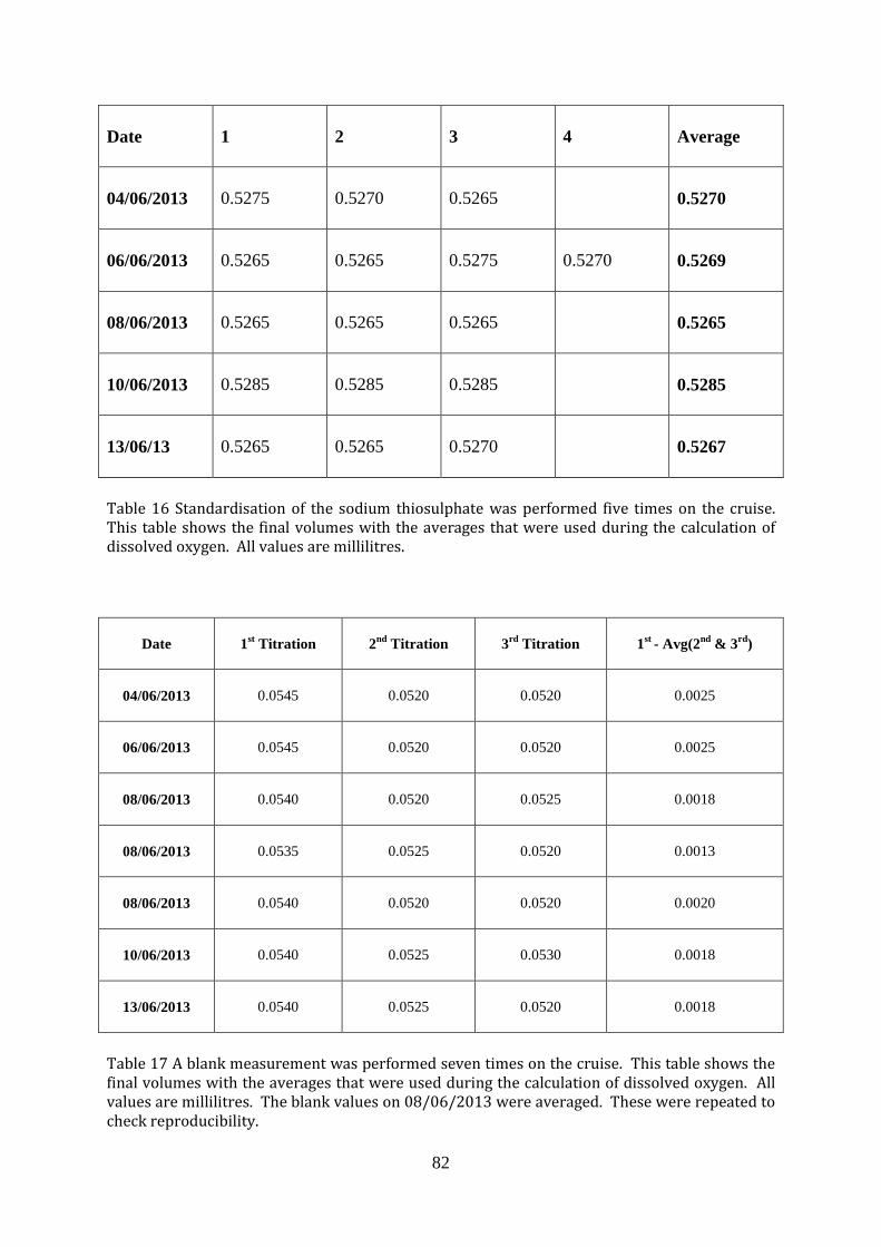
82

Date 1 2 3 4 Average

04/06/2013

0.5275 0.5270 0.5265 0.5270

06/06/2013

0.5265 0.5265 0.5275 0.5270 0.5269

08/06/2013

0.5265 0.5265 0.5265 0.5265

10/06/2013

0.5285 0.5285 0.5285 0.5285

13/06/13 0.5265 0.5265 0.5270 0.5267

Table 16 Standardisation of the sodium thiosulphate was performed five times on the cruise. This table shows the final volumes with the averages that were used during the calculation of dissolved oxygen. All values are millilitres.

Date

1st Titration 2nd Titration 3rd Titration 1st - Avg(2nd & 3rd)

04/06/2013

0.0545 0.0520 0.0520 0.0025

06/06/2013

0.0545 0.0520 0.0520 0.0025

08/06/2013

0.0540 0.0520 0.0525 0.0018

08/06/2013

0.0535 0.0525 0.0520 0.0013

08/06/2013

0.0540 0.0520 0.0520 0.0020

10/06/2013

0.0540 0.0525 0.0530 0.0018

13/06/2013

0.0540 0.0525 0.0520 0.0018

Table 17 A blank measurement was performed seven times on the cruise. This table shows the final volumes with the averages that were used during the calculation of dissolved oxygen. All values are millilitres. The blank values on 08/06/2013 were averaged. These were repeated to check reproducibility.

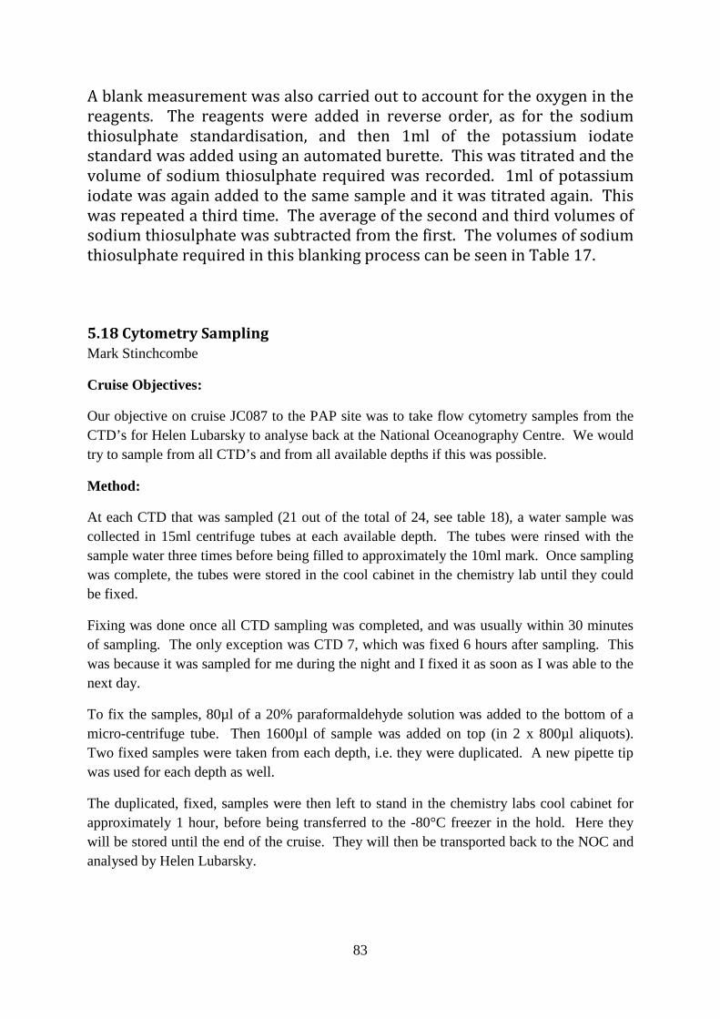
83

A blank measurement was also carried out to account for the oxygen in the reagents. The reagents were added in reverse order, as for the sodium thiosulphate standardisation, and then 1ml of the potassium iodate standard was added using an automated burette. This was titrated and the volume of sodium thiosulphate required was recorded. 1ml of potassium iodate was again added to the same sample and it was titrated again. This was repeated a third time. The average of the second and third volumes of sodium thiosulphate was subtracted from the first. The volumes of sodium thiosulphate required in this blanking process can be seen in Table 17.

5.18 Cytometry Sampling Mark Stinchcombe

Cruise Objectives:

Our objective on cruise JC087 to the PAP site was to take flow cytometry samples from the CTD’s for Helen Lubarsky to analyse back at the National Oceanography Centre. We would try to sample from all CTD’s and from all available depths if this was possible.

Method:

At each CTD that was sampled (21 out of the total of 24, see table 18), a water sample was collected in 15ml centrifuge tubes at each available depth. The tubes were rinsed with the sample water three times before being filled to approximately the 10ml mark. Once sampling was complete, the tubes were stored in the cool cabinet in the chemistry lab until they could be fixed.

Fixing was done once all CTD sampling was completed, and was usually within 30 minutes of sampling. The only exception was CTD 7, which was fixed 6 hours after sampling. This was because it was sampled for me during the night and I fixed it as soon as I was able to the next day.

To fix the samples, 80µl of a 20% paraformaldehyde solution was added to the bottom of a micro-centrifuge tube. Then 1600µl of sample was added on top (in 2 x 800µl aliquots). Two fixed samples were taken from each depth, i.e. they were duplicated. A new pipette tip was used for each depth as well.

The duplicated, fixed, samples were then left to stand in the chemistry labs cool cabinet for approximately 1 hour, before being transferred to the -80°C freezer in the hold. Here they will be stored until the end of the cruise. They will then be transported back to the NOC and analysed by Helen Lubarsky.

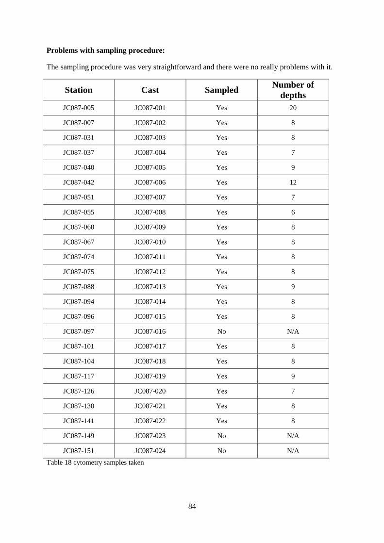
84

Problems with sampling procedure:

The sampling procedure was very straightforward and there were no really problems with it.

Station Cast Sampled Number of depths

JC087-005 JC087-001 Yes 20

JC087-007 JC087-002 Yes 8

JC087-031 JC087-003 Yes 8

JC087-037 JC087-004 Yes 7

JC087-040 JC087-005 Yes 9

JC087-042 JC087-006 Yes 12

JC087-051 JC087-007 Yes 7

JC087-055 JC087-008 Yes 6

JC087-060 JC087-009 Yes 8

JC087-067 JC087-010 Yes 8

JC087-074 JC087-011 Yes 8

JC087-075 JC087-012 Yes 8

JC087-088 JC087-013 Yes 9

JC087-094 JC087-014 Yes 8

JC087-096 JC087-015 Yes 8

JC087-097 JC087-016 No N/A

JC087-101 JC087-017 Yes 8

JC087-104 JC087-018 Yes 8

JC087-117 JC087-019 Yes 9

JC087-126 JC087-020 Yes 7

JC087-130 JC087-021 Yes 8

JC087-141 JC087-022 Yes 8

JC087-149 JC087-023 No N/A

JC087-151 JC087-024 No N/A Table 18 cytometry samples taken

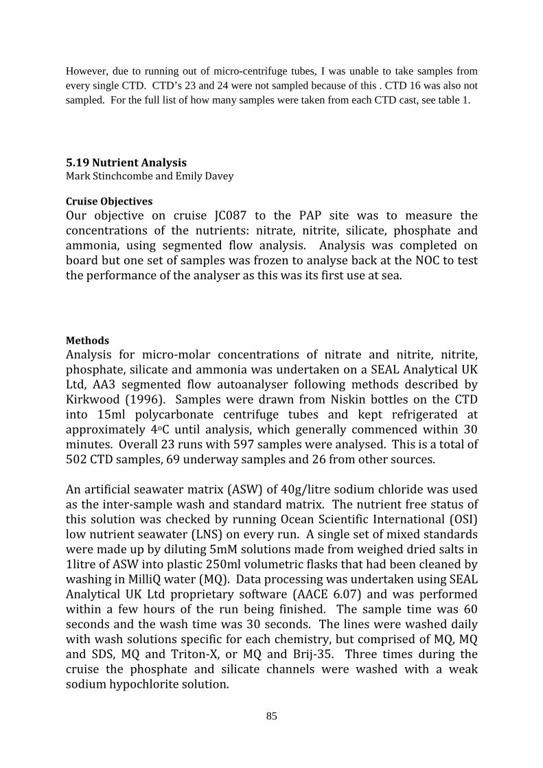
85

However, due to running out of micro-centrifuge tubes, I was unable to take samples from every single CTD. CTD’s 23 and 24 were not sampled because of this . CTD 16 was also not sampled. For the full list of how many samples were taken from each CTD cast, see table 1.

5.19 Nutrient Analysis Mark Stinchcombe and Emily Davey Cruise Objectives Our objective on cruise JC087 to the PAP site was to measure the concentrations of the nutrients: nitrate, nitrite, silicate, phosphate and ammonia, using segmented flow analysis. Analysis was completed on board but one set of samples was frozen to analyse back at the NOC to test the performance of the analyser as this was its first use at sea. Methods Analysis for micro-molar concentrations of nitrate and nitrite, nitrite, phosphate, silicate and ammonia was undertaken on a SEAL Analytical UK Ltd, AA3 segmented flow autoanalyser following methods described by Kirkwood (1996). Samples were drawn from Niskin bottles on the CTD into 15ml polycarbonate centrifuge tubes and kept refrigerated at approximately 4oC until analysis, which generally commenced within 30 minutes. Overall 23 runs with 597 samples were analysed. This is a total of 502 CTD samples, 69 underway samples and 26 from other sources. An artificial seawater matrix (ASW) of 40g/litre sodium chloride was used as the inter-sample wash and standard matrix. The nutrient free status of this solution was checked by running Ocean Scientific International (OSI) low nutrient seawater (LNS) on every run. A single set of mixed standards were made up by diluting 5mM solutions made from weighed dried salts in 1litre of ASW into plastic 250ml volumetric flasks that had been cleaned by washing in MilliQ water (MQ). Data processing was undertaken using SEAL Analytical UK Ltd proprietary software (AACE 6.07) and was performed within a few hours of the run being finished. The sample time was 60 seconds and the wash time was 30 seconds. The lines were washed daily with wash solutions specific for each chemistry, but comprised of MQ, MQ and SDS, MQ and Triton-X, or MQ and Brij-35. Three times during the cruise the phosphate and silicate channels were washed with a weak sodium hypochlorite solution.

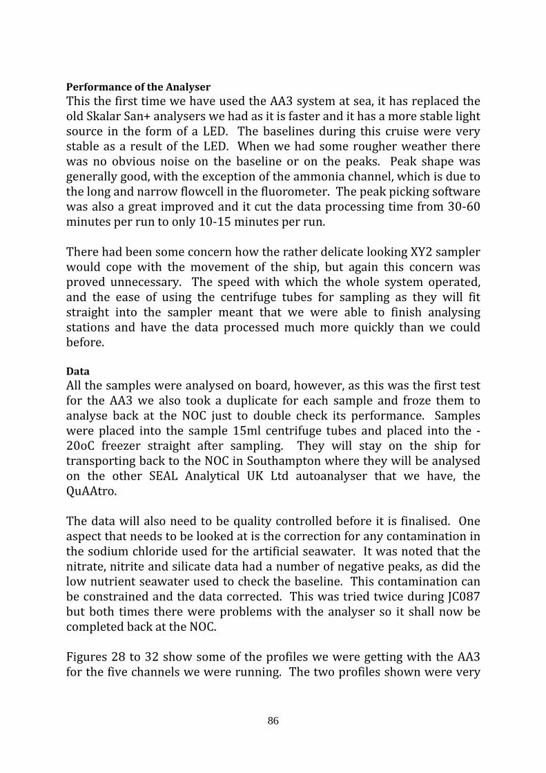
86

Performance of the Analyser This the first time we have used the AA3 system at sea, it has replaced the old Skalar San+ analysers we had as it is faster and it has a more stable light source in the form of a LED. The baselines during this cruise were very stable as a result of the LED. When we had some rougher weather there was no obvious noise on the baseline or on the peaks. Peak shape was generally good, with the exception of the ammonia channel, which is due to the long and narrow flowcell in the fluorometer. The peak picking software was also a great improved and it cut the data processing time from 30-60 minutes per run to only 10-15 minutes per run. There had been some concern how the rather delicate looking XY2 sampler would cope with the movement of the ship, but again this concern was proved unnecessary. The speed with which the whole system operated, and the ease of using the centrifuge tubes for sampling as they will fit straight into the sampler meant that we were able to finish analysing stations and have the data processed much more quickly than we could before.

Data All the samples were analysed on board, however, as this was the first test for the AA3 we also took a duplicate for each sample and froze them to analyse back at the NOC just to double check its performance. Samples were placed into the sample 15ml centrifuge tubes and placed into the -20oC freezer straight after sampling. They will stay on the ship for transporting back to the NOC in Southampton where they will be analysed on the other SEAL Analytical UK Ltd autoanalyser that we have, the QuAAtro. The data will also need to be quality controlled before it is finalised. One aspect that needs to be looked at is the correction for any contamination in the sodium chloride used for the artificial seawater. It was noted that the nitrate, nitrite and silicate data had a number of negative peaks, as did the low nutrient seawater used to check the baseline. This contamination can be constrained and the data corrected. This was tried twice during JC087 but both times there were problems with the analyser so it shall now be completed back at the NOC. Figures 28 to 32 show some of the profiles we were getting with the AA3 for the five channels we were running. The two profiles shown were very

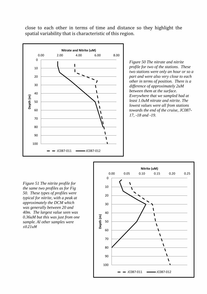
87

0

10

20

30

40

50

60

70

80

90

100

0.00 2.00 4.00 6.00 8.00

Dept

h (m

)

Nitrate and Nitrite (uM)

JC087-011 JC087-012

0

10

20

30

40

50

60

70

80

90

100

0.00 0.05 0.10 0.15 0.20 0.25

Dept

h (m

)

Nitrite (uM)

JC087-011 JC087-012

close to each other in terms of time and distance so they highlight the spatial variability that is characteristic of this region.

Figure 50 The nitrate and nitrite profile for two of the stations. These two stations were only an hour or so a part and were also very close to each other in terms of position. There is a difference of approximately 2uM between them at the surface. Everywhere that we sampled had at least 1.0uM nitrate and nitrite. The lowest values were all from stations towards the end of the cruise, JC087-17, -18 and -19.

Figure 51 The nitrite profile for the same two profiles as for Fig 50. These types of profiles were typical for nitrite, with a peak at approximately the DCM which was generally between 20 and 40m. The largest value seen was 0.36uM but this was just from one sample. Al other samples were ≤0.21uM

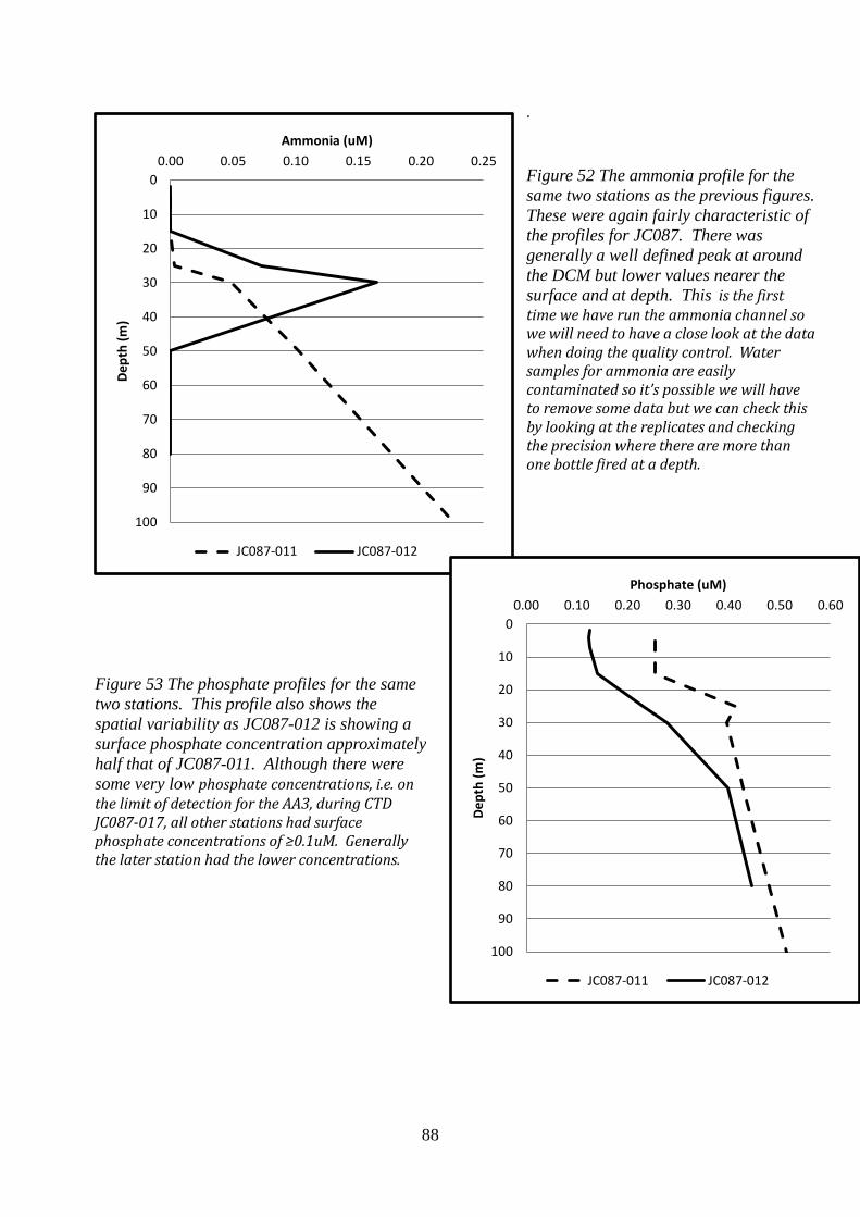
88

0

10

20

30

40

50

60

70

80

90

100

0.00 0.05 0.10 0.15 0.20 0.25

Dept

h (m

) Ammonia (uM)

JC087-011 JC087-012

0

10

20

30

40

50

60

70

80

90

100

0.00 0.10 0.20 0.30 0.40 0.50 0.60

Dept

h (m

)

Phosphate (uM)

JC087-011 JC087-012

.

Figure 52 The ammonia profile for the same two stations as the previous figures. These were again fairly characteristic of the profiles for JC087. There was generally a well defined peak at around the DCM but lower values nearer the surface and at depth. This is the first time we have run the ammonia channel so we will need to have a close look at the data when doing the quality control. Water samples for ammonia are easily contaminated so it’s possible we will have to remove some data but we can check this by looking at the replicates and checking the precision where there are more than one bottle fired at a depth.

Figure 53 The phosphate profiles for the same two stations. This profile also shows the spatial variability as JC087-012 is showing a surface phosphate concentration approximately half that of JC087-011. Although there were some very low phosphate concentrations, i.e. on the limit of detection for the AA3, during CTD JC087-017, all other stations had surface phosphate concentrations of ≥0.1uM. Generally the later station had the lower concentrations.

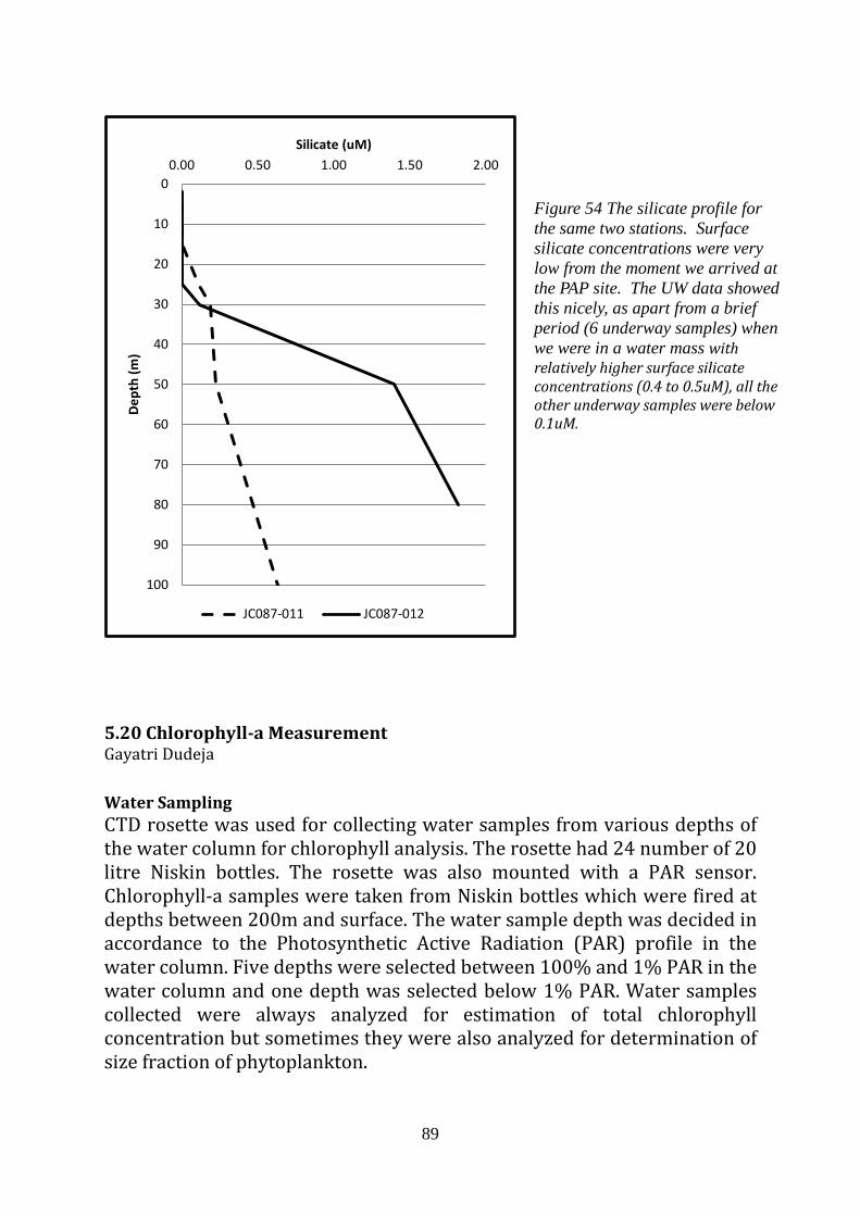
89

0

10

20

30

40

50

60

70

80

90

100

0.00 0.50 1.00 1.50 2.00

Dept

h (m

) Silicate (uM)

JC087-011 JC087-012

5.20 Chlorophyll-a Measurement Gayatri Dudeja Water Sampling CTD rosette was used for collecting water samples from various depths of the water column for chlorophyll analysis. The rosette had 24 number of 20 litre Niskin bottles. The rosette was also mounted with a PAR sensor. Chlorophyll-a samples were taken from Niskin bottles which were fired at depths between 200m and surface. The water sample depth was decided in accordance to the Photosynthetic Active Radiation (PAR) profile in the water column. Five depths were selected between 100% and 1% PAR in the water column and one depth was selected below 1% PAR. Water samples collected were always analyzed for estimation of total chlorophyll concentration but sometimes they were also analyzed for determination of size fraction of phytoplankton.

Figure 54 The silicate profile for the same two stations. Surface silicate concentrations were very low from the moment we arrived at the PAP site. The UW data showed this nicely, as apart from a brief period (6 underway samples) when we were in a water mass with relatively higher surface silicate concentrations (0.4 to 0.5uM), all the other underway samples were below 0.1uM.

90

Water samples for chlorophyll-a analysis were collected for various purposes- Pre-Dawn: As the name signifies, these samples were taken just before dawn i.e. at 4:00 am. This was to estimate chlorophyll concentration in the water before the water samples are incubated for primary production analysis. Water samples were taken from 6 Pre-Dawn CTD casts. The samples were analyzed for total chlorophyll concentration and also for determining the size fraction of phytoplankton in the water. Deep CTD: Two CTD casts were conducted with maximum depth of the cast more than 4500m. These casts were mainly done to match the glider.

5.21 Sea Mammal Sound Records Adrian Martin and Kevin Saw, with remote assistance from Douglas Gillespie and Mark Johnson of SMRU

Following a discussion with Douglas Gillespie of SMRU, a SMRU self-logging sound recorder was borrowed from SMRU and taken on JC87 for deployment on one of the Pelagra neutrally buoyant sediment traps. The idea behind this is that having no engine and, for the most part, residing at depth, the Pelagra potentially offers a very quiet environment to listen for cetacean calls and noises. Prior to the cruise the sensor was weighed in fresh water (89.5g) and one of the Pelagras (P8) was ballasted to accommodate it. Prior to deployment the sensor was connected to a laptop to charge. For the first deployment the time may not have been sufficient for it to charge fully. It was fully charged for the second. The computer was also used to ‘arm’ the sensor and synchronise its clock to that of the laptop which had itself already been synchronised with the ship clock. Both of these were accomplished using the d3host software provided by SMRU. At deployment the sensor was fastened with cable ties to one of the vertical plastic struts at the base of the Pelagra. This location was chosen as it is away from the top frame (where it may be damaged on recovery) and also distant from the central flotation rings (as hollow chambers potentially offer a source of noise). The loose nuts used as ballast were also cable-tied together where possible to minimise any noise arising from their banging together.

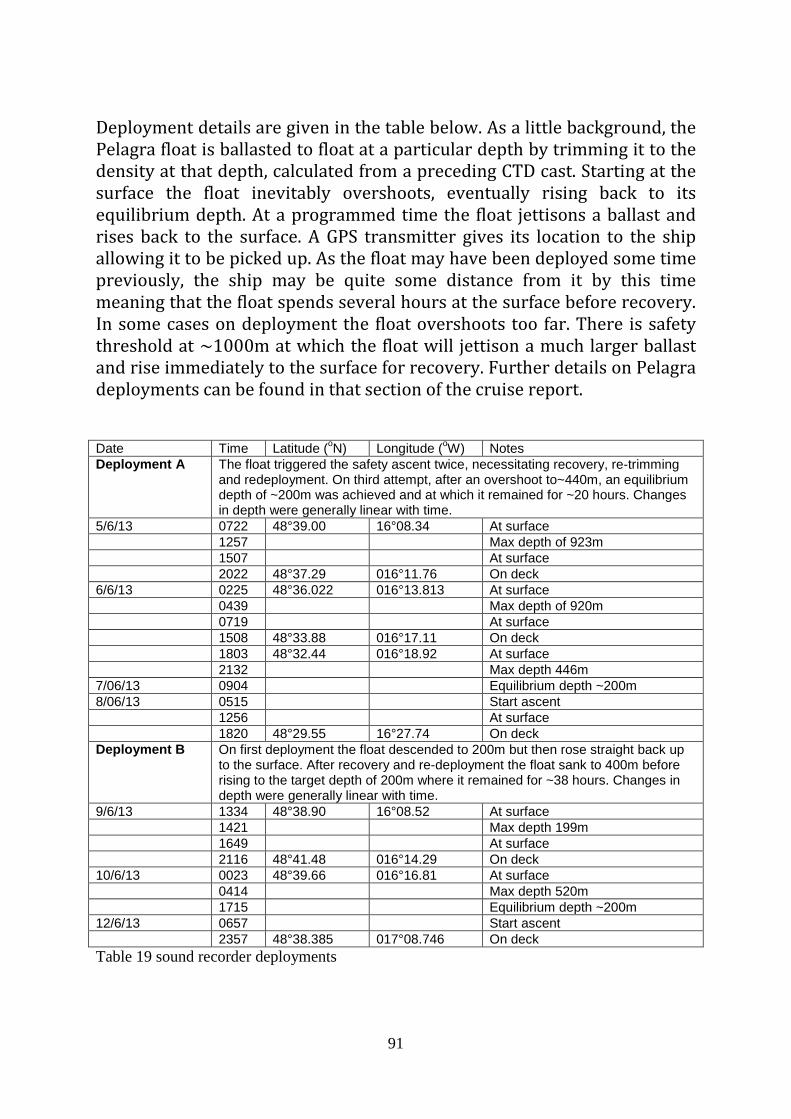
91

Deployment details are given in the table below. As a little background, the Pelagra float is ballasted to float at a particular depth by trimming it to the density at that depth, calculated from a preceding CTD cast. Starting at the surface the float inevitably overshoots, eventually rising back to its equilibrium depth. At a programmed time the float jettisons a ballast and rises back to the surface. A GPS transmitter gives its location to the ship allowing it to be picked up. As the float may have been deployed some time previously, the ship may be quite some distance from it by this time meaning that the float spends several hours at the surface before recovery. In some cases on deployment the float overshoots too far. There is safety threshold at ~1000m at which the float will jettison a much larger ballast and rise immediately to the surface for recovery. Further details on Pelagra deployments can be found in that section of the cruise report. Date Time Latitude (oN) Longitude (oW) Notes Deployment A The float triggered the safety ascent twice, necessitating recovery, re-trimming

and redeployment. On third attempt, after an overshoot to~440m, an equilibrium depth of ~200m was achieved and at which it remained for ~20 hours. Changes in depth were generally linear with time.

5/6/13 0722 48°39.00 16°08.34 At surface 1257 Max depth of 923m 1507 At surface 2022 48°37.29 016°11.76 On deck 6/6/13 0225 48°36.022 016°13.813 At surface 0439 Max depth of 920m 0719 At surface 1508 48°33.88 016°17.11 On deck 1803 48°32.44 016°18.92 At surface 2132 Max depth 446m 7/06/13 0904 Equilibrium depth ~200m 8/06/13 0515 Start ascent 1256 At surface 1820 48°29.55 16°27.74 On deck Deployment B On first deployment the float descended to 200m but then rose straight back up

to the surface. After recovery and re-deployment the float sank to 400m before rising to the target depth of 200m where it remained for ~38 hours. Changes in depth were generally linear with time.

9/6/13 1334 48°38.90 16°08.52 At surface 1421 Max depth 199m 1649 At surface 2116 48°41.48 016°14.29 On deck 10/6/13 0023 48°39.66 016°16.81 At surface 0414 Max depth 520m 1715 Equilibrium depth ~200m 12/6/13 0657 Start ascent 2357 48°38.385 017°08.746 On deck Table 19 sound recorder deployments

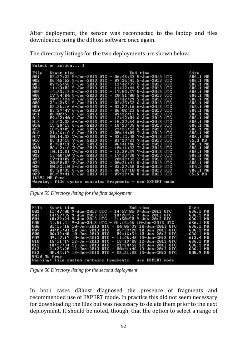
92

After deployment, the sensor was reconnected to the laptop and files downloaded using the d3host software once again. The directory listings for the two deployments are shown below.

Figure 55 Directory listing for the first deployment

Figure 56 Directory listing for the second deployment

In both cases d3host diagnosed the presence of fragments and recommended use of EXPERT mode. In practice this did not seem necessary for downloading the files but was necessary to delete them prior to the next deployment. It should be noted, though, that the option to select a range of

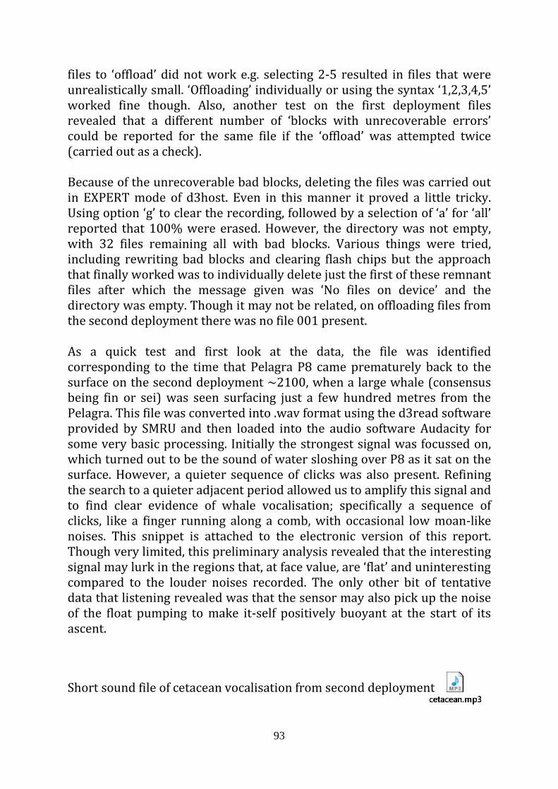
93

files to ‘offload’ did not work e.g. selecting 2-5 resulted in files that were unrealistically small. ‘Offloading’ individually or using the syntax ‘1,2,3,4,5’ worked fine though. Also, another test on the first deployment files revealed that a different number of ‘blocks with unrecoverable errors’ could be reported for the same file if the ‘offload’ was attempted twice (carried out as a check). Because of the unrecoverable bad blocks, deleting the files was carried out in EXPERT mode of d3host. Even in this manner it proved a little tricky. Using option ‘g’ to clear the recording, followed by a selection of ‘a’ for ‘all’ reported that 100% were erased. However, the directory was not empty, with 32 files remaining all with bad blocks. Various things were tried, including rewriting bad blocks and clearing flash chips but the approach that finally worked was to individually delete just the first of these remnant files after which the message given was ‘No files on device’ and the directory was empty. Though it may not be related, on offloading files from the second deployment there was no file 001 present. As a quick test and first look at the data, the file was identified corresponding to the time that Pelagra P8 came prematurely back to the surface on the second deployment ~2100, when a large whale (consensus being fin or sei) was seen surfacing just a few hundred metres from the Pelagra. This file was converted into .wav format using the d3read software provided by SMRU and then loaded into the audio software Audacity for some very basic processing. Initially the strongest signal was focussed on, which turned out to be the sound of water sloshing over P8 as it sat on the surface. However, a quieter sequence of clicks was also present. Refining the search to a quieter adjacent period allowed us to amplify this signal and to find clear evidence of whale vocalisation; specifically a sequence of clicks, like a finger running along a comb, with occasional low moan-like noises. This snippet is attached to the electronic version of this report. Though very limited, this preliminary analysis revealed that the interesting signal may lurk in the regions that, at face value, are ‘flat’ and uninteresting compared to the louder noises recorded. The only other bit of tentative data that listening revealed was that the sensor may also pick up the noise of the float pumping to make it-self positively buoyant at the start of its ascent. Short sound file of cetacean vocalisation from second deployment

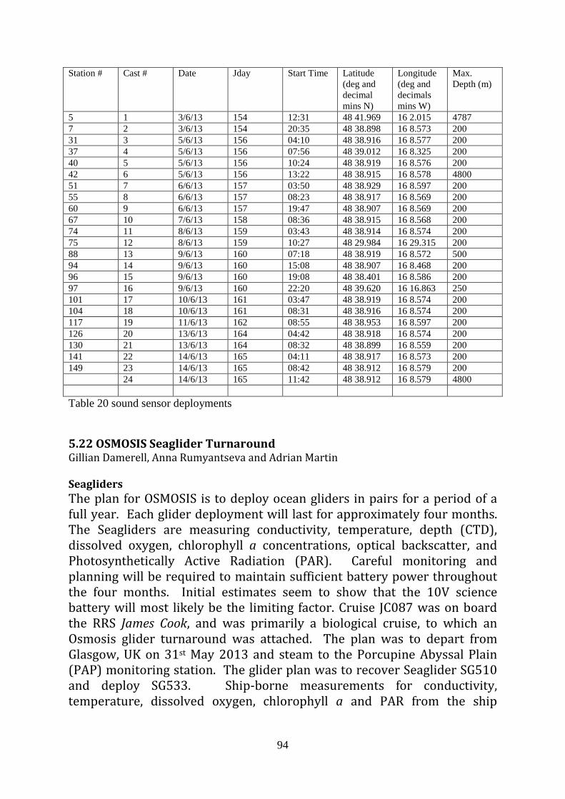
94

Station # Cast # Date Jday Start Time Latitude (deg and decimal mins N)

Longitude (deg and decimals mins W)

Max. Depth (m)

5 1 3/6/13 154 12:31 48 41.969 16 2.015 4787 7 2 3/6/13 154 20:35 48 38.898 16 8.573 200 31 3 5/6/13 156 04:10 48 38.916 16 8.577 200 37 4 5/6/13 156 07:56 48 39.012 16 8.325 200 40 5 5/6/13 156 10:24 48 38.919 16 8.576 200 42 6 5/6/13 156 13:22 48 38.915 16 8.578 4800 51 7 6/6/13 157 03:50 48 38.929 16 8.597 200 55 8 6/6/13 157 08:23 48 38.917 16 8.569 200 60 9 6/6/13 157 19:47 48 38.907 16 8.569 200 67 10 7/6/13 158 08:36 48 38.915 16 8.568 200 74 11 8/6/13 159 03:43 48 38.914 16 8.574 200 75 12 8/6/13 159 10:27 48 29.984 16 29.315 200 88 13 9/6/13 160 07:18 48 38.919 16 8.572 500 94 14 9/6/13 160 15:08 48 38.907 16 8.468 200 96 15 9/6/13 160 19:08 48 38.401 16 8.586 200 97 16 9/6/13 160 22:20 48 39.620 16 16.863 250 101 17 10/6/13 161 03:47 48 38.919 16 8.574 200 104 18 10/6/13 161 08:31 48 38.916 16 8.574 200 117 19 11/6/13 162 08:55 48 38.953 16 8.597 200 126 20 13/6/13 164 04:42 48 38.918 16 8.574 200 130 21 13/6/13 164 08:32 48 38.899 16 8.559 200 141 22 14/6/13 165 04:11 48 38.917 16 8.573 200 149 23 14/6/13 165 08:42 48 38.912 16 8.579 200 24 14/6/13 165 11:42 48 38.912 16 8.579 4800 Table 20 sound sensor deployments 5.22 OSMOSIS Seaglider Turnaround Gillian Damerell, Anna Rumyantseva and Adrian Martin Seagliders The plan for OSMOSIS is to deploy ocean gliders in pairs for a period of a full year. Each glider deployment will last for approximately four months. The Seagliders are measuring conductivity, temperature, depth (CTD), dissolved oxygen, chlorophyll a concentrations, optical backscatter, and Photosynthetically Active Radiation (PAR). Careful monitoring and planning will be required to maintain sufficient battery power throughout the four months. Initial estimates seem to show that the 10V science battery will most likely be the limiting factor. Cruise JC087 was on board the RRS James Cook, and was primarily a biological cruise, to which an Osmosis glider turnaround was attached. The plan was to depart from Glasgow, UK on 31st May 2013 and steam to the Porcupine Abyssal Plain (PAP) monitoring station. The glider plan was to recover Seaglider SG510 and deploy SG533. Ship-borne measurements for conductivity, temperature, dissolved oxygen, chlorophyll a and PAR from the ship

95

deployed CTD rosette will be used to calibrate the sensors on the Seagliders. Timeline of glider-related activities 30th May 2013 Came on board ship, ran self-test 23 and sim dives 6 and

7 on SG533. Checked Argos tag. 31st May 2013 Sailed from Govan, Glasgow, assembled SG533, opened

hatches, checked cables all tight, closed hatches 1st June 2013 Recovered Fastnet Slocum glider with a leak, checked

SG533 self-test and sim dives for errors 2nd June 2013 Updated cmdfile for deployment, including calibration

constants for new CT sail – which later proved to be wildly wrong. Piloting team at UEA corrected after deployment. Ran and checked self-test 24 and sim dive 8.

3rd June 2013 Station 001, deployment of SG533 Station 005, CTD cast 001: ship deployed CTD to 4787m for Seaglider calibration and lipid sampling

9th June 2013 Recovery of SG510 Station 088, CTD cast 013: ship deployed CTD to 500m for Seaglider calibration

14th June 2013 Begin transit to Govan, Glasgow for the end of cruise demobilisation

18th June 2013 Dock in Govan, Glasgow Preparation The team arrived at the ship on the 30th of May. SG533 (Canopus), and the crate for SG510, were already loaded on the RRS James Cook when we boarded, both on the back deck. Communications We began by switching on SG533 and running a self-test and two sim dives, using NOCS PSTN as the primary phone number and UEA PSTN as the alternative. On the 2nd June, we changed this to be NOCS RUDICS as the primary phone number and NOCS PSTN as the alternative number. Communications were good with both NOCS RUDICS and NOCS PSTN, with the glider lying flat on the back deck with the antenna propped up vertically, or with the glider propped up against the rail of the ship with the antenna fastened in place in the glider. We did not test communications using the UEA PSTN line, noting that it had already displayed problems for SG566’s communications. The appropriate numbers are:

96

NOCS RUDICS: 881600005139 NOCS PSTN: 442380634452 UEA PSTN: 441603597331 Self-tests and Simulated Dives Multiple self-tests and sim dives were carried out on SG533. The only errors that were encountered involved bathymetry maps and the ability to pick up a GPS signal. The former is not relevant for this project as the water depth is more than 4000m in this area, and the latter is an expected error due to the short period of time that is allowed to obtain a GPS fix during the self test (see Seaglider manual). Upon going through the iRobot provided checklist of the self tests and sim dives, we noticed, in the tests carried out on 30th May that the pitch was much lower than recommended. This is because we had the glider positioned flat on the back deck rather than propped up against the rail of the ship. Self-test 24 and sim dive 8 showed pitch angles appropriate for a glider propped up against the rail. We also noticed that SG533’s VBD was pumping at a rate of 4 to 5 AD/sec, whereas rates greater than or equal to 7 AD/sec are expected. This also occurred for SG566 during the September 2012 deployment, and on that occasion we were advised by iRobot to set both $D_BOOST and $T_BOOST to 0, which allows both the main pump and the boost pump to work in tandem. This was altered for sim dive 8, whereupon the pumping rate increased to 11 AD/sec. All self tests were screen logged on Gillian’s laptop. Assembly The glider was brought into the main lab where we attached the wings, rudder and antenna. With memories of the loose cables found in the September 2012 deployment, we opened the front and back hatches and checked that all the cables which pass into the pressure hull were tightly attached. Acoustic Deck Box We interrogated the glider with the acoustic deck box and received a good reading. The interrogation and return frequencies for SG533 are: SG533: Interrogate, 13.0; Respond, 11.5 Argos Tag The Argos tag had previously been set up by Gareth Lee et al. on JC085. We merely attached the tag to a laptop to check it was still functional.

97

Deployment Deploying and recovering Seagliders is always best achieved with the use of a small boat, but this is not always possible. Sea conditions may not be suitable, or the use of a small boat on a large research vessel may be strictly limited to rescue operations (i.e., such a boat is not a work boat). When Seagliders are deployed from ships, a winch is required to lower them into the water. On the RRS James Cook, the Rexroth winch (located on the Starboard A frame) was used to lower them into the water. The Rigid Rope Technique The Rigid Rope technique involves passing a length of rope through two 2m lengths of 25mm flexi-pipe, as used in household plumbing. The 2m lengths of flexi-pipe act as a sheath to keep the rope rigid and eliminate tangling around the antenna. Loops are tied at either to act as a means of fixing the rope to the winch/Sea-Catch release mechanism. The Seaglider then sits between the two lengths of pipe, creating a sling through which the Seaglider can be supported during winch operations. A sea-catch release hook is attached to the end of the winch and one loop of the sling is permanently fixed to the wire with a shackle and cannot be released. The other loop is attached to the release eye of the sea-catch. When the deployment team is satisfied that the Seaglider is ready to deploy, the sea-catch releases the Seaglider. This technique was developed by Gareth Lee for JC085. We had intended to carry out a separate buoyancy test by using a cable tie to bind the two ropes together and prevent release of the Seaglider, then bring the glider back on deck. If the buoyancy test was satisfactory, we would then remove the cable tie and deploy straight away. However, the cable tie used was not sufficiently heavy duty and snapped when we started the raise the glider out of the water. The buoyancy had appeared satisfactory so we simply released the Seaglider from the sling without bringing it back on deck.

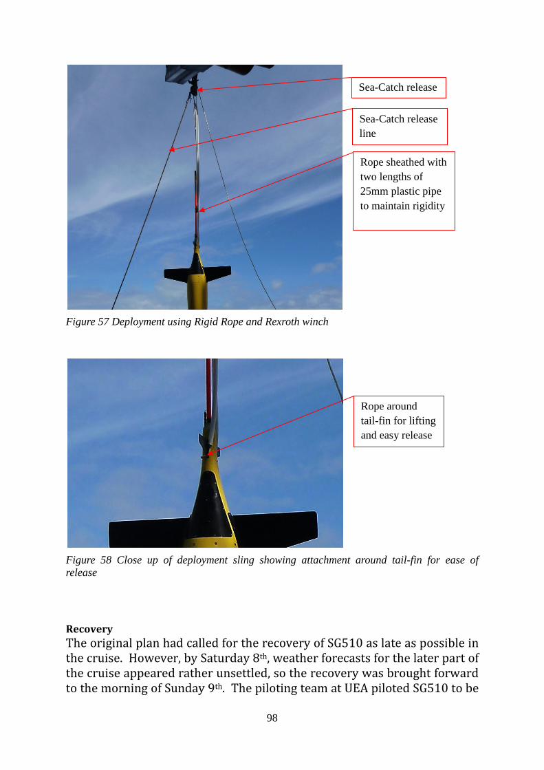
98

Figure 57 Deployment using Rigid Rope and Rexroth winch

Figure 58 Close up of deployment sling showing attachment around tail-fin for ease of release Recovery The original plan had called for the recovery of SG510 as late as possible in the cruise. However, by Saturday 8th, weather forecasts for the later part of the cruise appeared rather unsettled, so the recovery was brought forward to the morning of Sunday 9th. The piloting team at UEA piloted SG510 to be

Sea-Catch release

Rope sheathed with two lengths of 25mm plastic pipe to maintain rigidity

Sea-Catch release line

Rope around tail-fin for lifting and easy release

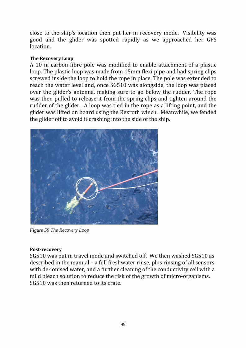
99

close to the ship’s location then put her in recovery mode. Visibility was good and the glider was spotted rapidly as we approached her GPS location. The Recovery Loop A 10 m carbon fibre pole was modified to enable attachment of a plastic loop. The plastic loop was made from 15mm flexi pipe and had spring clips screwed inside the loop to hold the rope in place. The pole was extended to reach the water level and, once SG510 was alongside, the loop was placed over the glider’s antenna, making sure to go below the rudder. The rope was then pulled to release it from the spring clips and tighten around the rudder of the glider. A loop was tied in the rope as a lifting point, and the glider was lifted on board using the Rexroth winch. Meanwhile, we fended the glider off to avoid it crashing into the side of the ship.

Figure 59 The Recovery Loop

Post-recovery SG510 was put in travel mode and switched off. We then washed SG510 as described in the manual – a full freshwater rinse, plus rinsing of all sensors with de-ionised water, and a further cleaning of the conductivity cell with a mild bleach solution to reduce the risk of the growth of micro-organisms. SG510 was then returned to its crate.

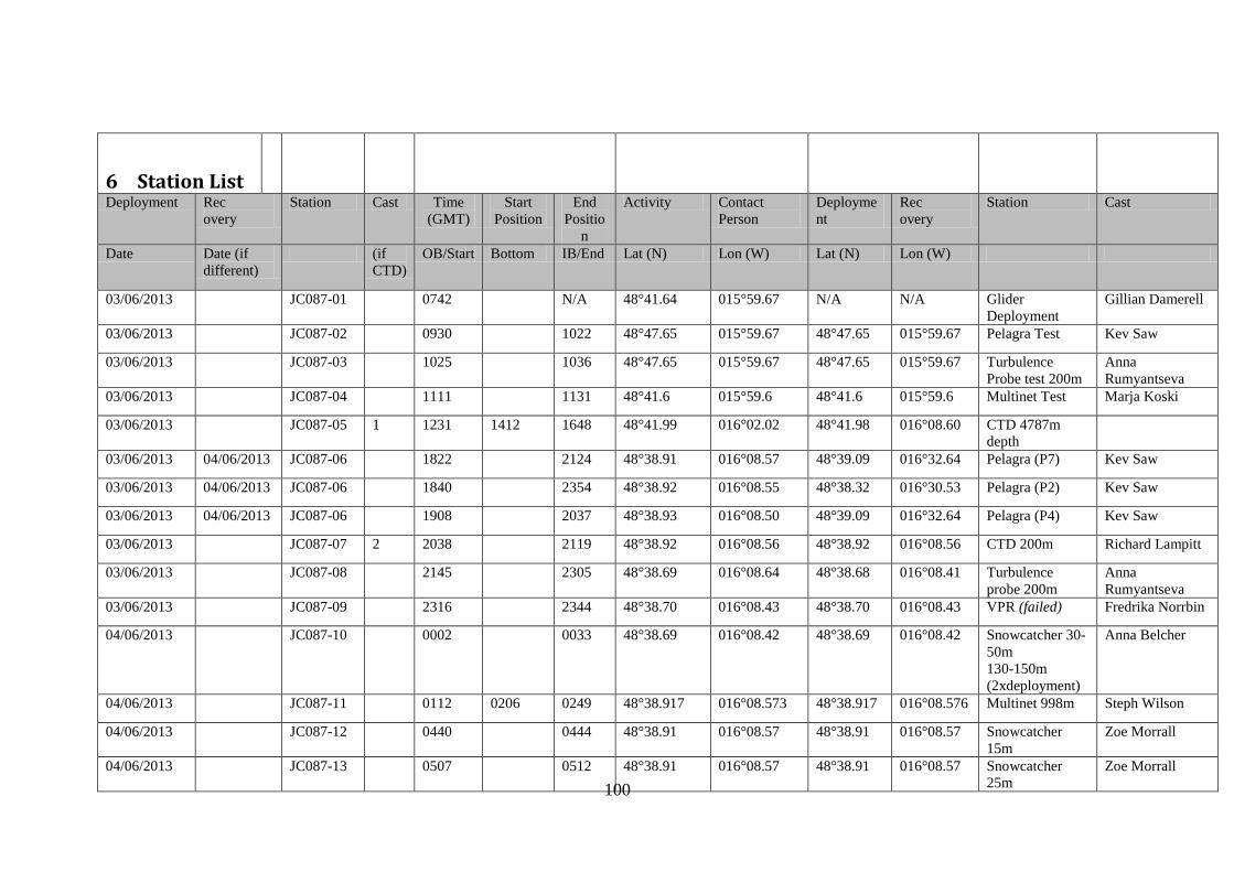
100

6 Station List

Deployment Rec overy

Station Cast Time (GMT)

Start Position

End Positio

n

Activity Contact Person

Deployment

Rec overy

Station Cast

Date Date (if different)

(if CTD)

OB/Start Bottom IB/End Lat (N) Lon (W) Lat (N) Lon (W)

03/06/2013 JC087-01 0742 N/A 48°41.64 015°59.67 N/A N/A Glider Deployment

Gillian Damerell

03/06/2013 JC087-02 0930 1022 48°47.65 015°59.67 48°47.65 015°59.67 Pelagra Test Kev Saw

03/06/2013 JC087-03 1025 1036 48°47.65 015°59.67 48°47.65 015°59.67 Turbulence Probe test 200m

Anna Rumyantseva

03/06/2013 JC087-04 1111 1131 48°41.6 015°59.6 48°41.6 015°59.6 Multinet Test Marja Koski

03/06/2013 JC087-05 1 1231 1412 1648 48°41.99 016°02.02 48°41.98 016°08.60 CTD 4787m depth

03/06/2013 04/06/2013 JC087-06 1822 2124 48°38.91 016°08.57 48°39.09 016°32.64 Pelagra (P7) Kev Saw

03/06/2013 04/06/2013 JC087-06 1840 2354 48°38.92 016°08.55 48°38.32 016°30.53 Pelagra (P2) Kev Saw

03/06/2013 04/06/2013 JC087-06 1908 2037 48°38.93 016°08.50 48°39.09 016°32.64 Pelagra (P4) Kev Saw

03/06/2013 JC087-07 2 2038 2119 48°38.92 016°08.56 48°38.92 016°08.56 CTD 200m Richard Lampitt

03/06/2013 JC087-08 2145 2305 48°38.69 016°08.64 48°38.68 016°08.41 Turbulence probe 200m

Anna Rumyantseva

03/06/2013 JC087-09 2316 2344 48°38.70 016°08.43 48°38.70 016°08.43 VPR (failed) Fredrika Norrbin

04/06/2013 JC087-10 0002 0033 48°38.69 016°08.42 48°38.69 016°08.42 Snowcatcher 30-50m 130-150m (2xdeployment)

Anna Belcher

04/06/2013 JC087-11 0112 0206 0249 48°38.917 016°08.573 48°38.917 016°08.576 Multinet 998m Steph Wilson

04/06/2013 JC087-12 0440 0444 48°38.91 016°08.57 48°38.91 016°08.57 Snowcatcher 15m

Zoe Morrall

04/06/2013 JC087-13 0507 0512 48°38.91 016°08.57 48°38.91 016°08.57 Snowcatcher 25m

Zoe Morrall

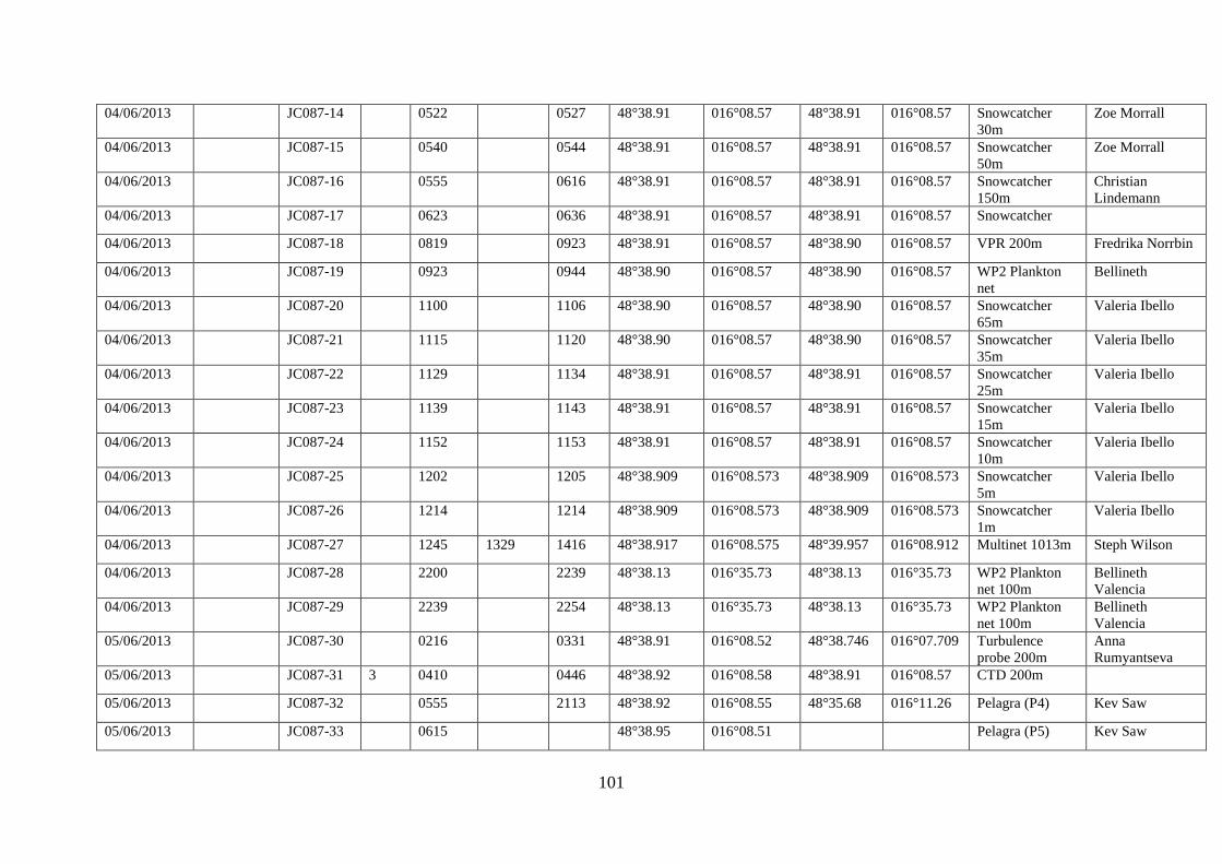
101

04/06/2013 JC087-14 0522 0527 48°38.91 016°08.57 48°38.91 016°08.57 Snowcatcher 30m

Zoe Morrall

04/06/2013 JC087-15 0540 0544 48°38.91 016°08.57 48°38.91 016°08.57 Snowcatcher 50m

Zoe Morrall

04/06/2013 JC087-16 0555 0616 48°38.91 016°08.57 48°38.91 016°08.57 Snowcatcher 150m

Christian Lindemann

04/06/2013 JC087-17 0623 0636 48°38.91 016°08.57 48°38.91 016°08.57 Snowcatcher

04/06/2013 JC087-18 0819 0923 48°38.91 016°08.57 48°38.90 016°08.57 VPR 200m Fredrika Norrbin

04/06/2013 JC087-19 0923 0944 48°38.90 016°08.57 48°38.90 016°08.57 WP2 Plankton net

Bellineth

04/06/2013 JC087-20 1100 1106 48°38.90 016°08.57 48°38.90 016°08.57 Snowcatcher 65m

Valeria Ibello

04/06/2013 JC087-21 1115 1120 48°38.90 016°08.57 48°38.90 016°08.57 Snowcatcher 35m

Valeria Ibello

04/06/2013 JC087-22 1129 1134 48°38.91 016°08.57 48°38.91 016°08.57 Snowcatcher 25m

Valeria Ibello

04/06/2013 JC087-23 1139 1143 48°38.91 016°08.57 48°38.91 016°08.57 Snowcatcher 15m

Valeria Ibello

04/06/2013 JC087-24 1152 1153 48°38.91 016°08.57 48°38.91 016°08.57 Snowcatcher 10m

Valeria Ibello

04/06/2013 JC087-25 1202 1205 48°38.909 016°08.573 48°38.909 016°08.573 Snowcatcher 5m

Valeria Ibello

04/06/2013 JC087-26 1214 1214 48°38.909 016°08.573 48°38.909 016°08.573 Snowcatcher 1m

Valeria Ibello

04/06/2013 JC087-27 1245 1329 1416 48°38.917 016°08.575 48°39.957 016°08.912 Multinet 1013m Steph Wilson

04/06/2013 JC087-28 2200 2239 48°38.13 016°35.73 48°38.13 016°35.73 WP2 Plankton net 100m

Bellineth Valencia

04/06/2013 JC087-29 2239 2254 48°38.13 016°35.73 48°38.13 016°35.73 WP2 Plankton net 100m

Bellineth Valencia

05/06/2013 JC087-30 0216 0331 48°38.91 016°08.52 48°38.746 016°07.709 Turbulence probe 200m

Anna Rumyantseva

05/06/2013 JC087-31 3 0410 0446 48°38.92 016°08.58 48°38.91 016°08.57 CTD 200m

05/06/2013 JC087-32 0555 2113 48°38.92 016°08.55 48°35.68 016°11.26 Pelagra (P4) Kev Saw

05/06/2013 JC087-33 0615 48°38.95 016°08.51 Pelagra (P5) Kev Saw

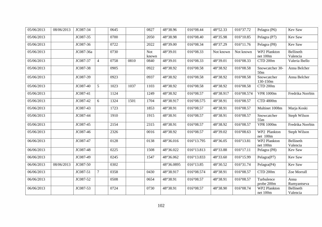
102

05/06/2013 08/06/2013 JC087-34 0645 0827 48°38.96 016°08.44 48°52.33 016°37.72 Pelagra (P6) Kev Saw

05/06/2013 JC087-35 0700 2050 48°38.98 016°08.40 48°35.98 016°10.85 Pelagra (P7) Kev Saw

05/06/2013 JC087-36 0722 2022 48°39.00 016°08.34 48°37.29 016°11.76 Pelagra (P8) Kev Saw

05/06/2013 JC087-36a 0730 Not known

48°39.01 016°08.33 Not known Not known WP2 Plankton net 100m

Bellineth Valencia

05/06/2013 JC087-37 4 0758 0810 0840 48°39.01 016°08.33 48°39.01 016°08.33 CTD 200m Valeria Ibello

05/06/2013 JC087-38 0905 0922 48°38.92 016°08.58 48°38.92 016°08.58 Snowcatcher 30-50m

Anna Belcher

05/06/2013 JC087-39 0923 0937 48°38.92 016°08.58 48°38.92 016°08.58 Snowcatcher 130-150m

Anna Belcher

05/06/2013 JC087-40 5 1023 1037 1103 48°38.92 016°08.58 48°38.92 016°08.58 CTD 200m

05/06/2013 JC087-41 1124 1249 48°38.92 016°08.57 48°38.917 016°08.574 VPR 1000m Fredrika Norrbin

05/06/2013 JC087-42 6 1324 1501 1704 48°38.917 016°08.575 48°38.91 016°08.57 CTD 4800m

05/06/2013 JC087-43 1723 1853 48°38.91 016°08.57 48°38.91 016°08.57 Multinet 1008m Marja Koski

05/06/2013 JC087-44 1910 1915 48°38.91 016°08.57 48°38.91 016°08.57 Snowcatcher 55m

Steph Wilson

05/06/2013 JC087-45 2154 2315 48°38.91 016°08.57 48°38.92 016°08.57 VPR 1000m Fredrika Norrbin

05/06/2013 JC087-46 2326 0016 48°38.92 016°08.57 48°39.02 016°08.63 WP2 Plankton net 100m

Steph Wilson

06/06/2013 JC087-47 0128 0138 48°36.016 016°13.795 48°36.05 016°13.81 WP2 Plankton net 100m

Bellineth Valencia

06/06/2013 JC087-48 0225 1508 48°36.022 016°13.813 48°33.88 016°17.11 Pelagra (P8) Kev Saw

06/06/2013 JC087-49 0245 1547 48°36.062 016°13.833 48°33.60 016°15.99 Pelagra(P7) Kev Saw

06/06/2013 08/06/2013 JC087-50 0302 48°36.0895 016°13.85 48°30.52 016°31.74 Pelagra(P4) Kev Saw

06/06/2013 JC087-51 7 0358 0430 48°38.917 016°08.574 48°38.91 016°08.57 CTD 200m Zoe Morrall

06/06/2013 JC087-52 0508 0654 48°38.91 016°08.57 48°38.91 016°08.57 Turbulence probe 200m

Anna Rumyantseva

06/06/2013 JC087-53 0724 0730 48°38.91 016°08.57 48°38.90 016°08.74 WP2 Plankton net 100m

Bellineth Valencia

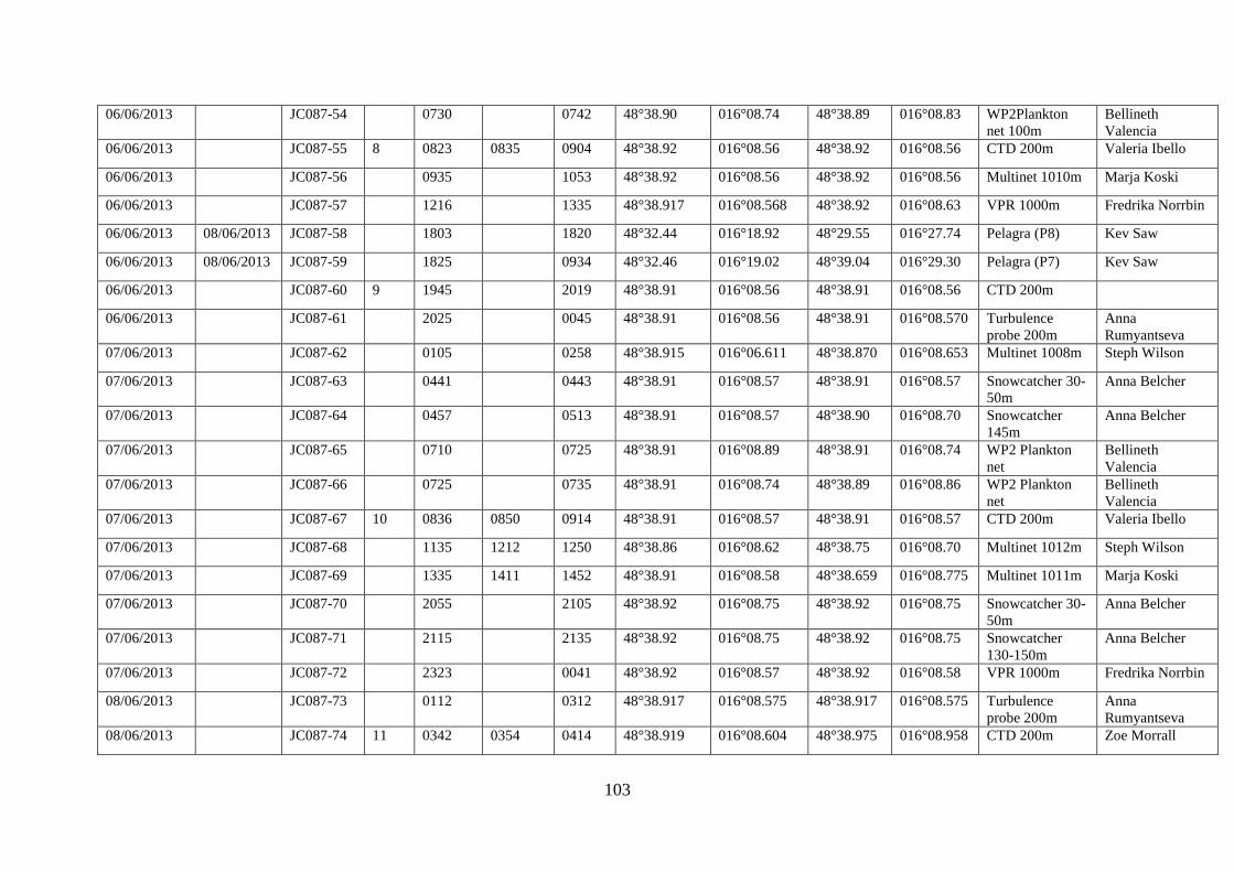
103

06/06/2013 JC087-54 0730 0742 48°38.90 016°08.74 48°38.89 016°08.83 WP2Plankton net 100m

Bellineth Valencia

06/06/2013 JC087-55 8 0823 0835 0904 48°38.92 016°08.56 48°38.92 016°08.56 CTD 200m Valeria Ibello

06/06/2013 JC087-56 0935 1053 48°38.92 016°08.56 48°38.92 016°08.56 Multinet 1010m Marja Koski

06/06/2013 JC087-57 1216 1335 48°38.917 016°08.568 48°38.92 016°08.63 VPR 1000m Fredrika Norrbin

06/06/2013 08/06/2013 JC087-58 1803 1820 48°32.44 016°18.92 48°29.55 016°27.74 Pelagra (P8) Kev Saw

06/06/2013 08/06/2013 JC087-59 1825 0934 48°32.46 016°19.02 48°39.04 016°29.30 Pelagra (P7) Kev Saw

06/06/2013 JC087-60 9 1945 2019 48°38.91 016°08.56 48°38.91 016°08.56 CTD 200m

06/06/2013 JC087-61 2025 0045 48°38.91 016°08.56 48°38.91 016°08.570 Turbulence probe 200m

Anna Rumyantseva

07/06/2013 JC087-62 0105 0258 48°38.915 016°06.611 48°38.870 016°08.653 Multinet 1008m Steph Wilson

07/06/2013 JC087-63 0441 0443 48°38.91 016°08.57 48°38.91 016°08.57 Snowcatcher 30-50m

Anna Belcher

07/06/2013 JC087-64 0457 0513 48°38.91 016°08.57 48°38.90 016°08.70 Snowcatcher 145m

Anna Belcher

07/06/2013 JC087-65 0710 0725 48°38.91 016°08.89 48°38.91 016°08.74 WP2 Plankton net

Bellineth Valencia

07/06/2013 JC087-66 0725 0735 48°38.91 016°08.74 48°38.89 016°08.86 WP2 Plankton net

Bellineth Valencia

07/06/2013 JC087-67 10 0836 0850 0914 48°38.91 016°08.57 48°38.91 016°08.57 CTD 200m Valeria Ibello

07/06/2013 JC087-68 1135 1212 1250 48°38.86 016°08.62 48°38.75 016°08.70 Multinet 1012m Steph Wilson

07/06/2013 JC087-69 1335 1411 1452 48°38.91 016°08.58 48°38.659 016°08.775 Multinet 1011m Marja Koski

07/06/2013 JC087-70 2055 2105 48°38.92 016°08.75 48°38.92 016°08.75 Snowcatcher 30-50m

Anna Belcher

07/06/2013 JC087-71 2115 2135 48°38.92 016°08.75 48°38.92 016°08.75 Snowcatcher 130-150m

Anna Belcher

07/06/2013 JC087-72 2323 0041 48°38.92 016°08.57 48°38.92 016°08.58 VPR 1000m Fredrika Norrbin

08/06/2013 JC087-73 0112 0312 48°38.917 016°08.575 48°38.917 016°08.575 Turbulence probe 200m

Anna Rumyantseva

08/06/2013 JC087-74 11 0342 0354 0414 48°38.919 016°08.604 48°38.975 016°08.958 CTD 200m Zoe Morrall

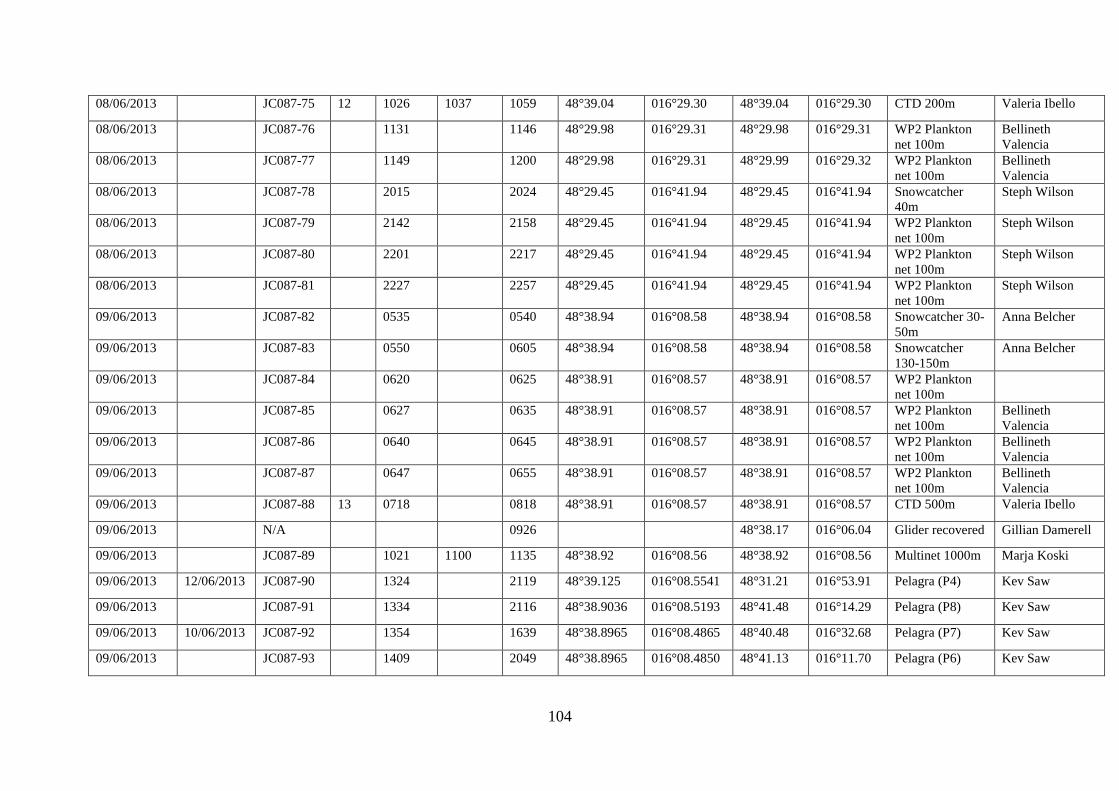
104

08/06/2013 JC087-75 12 1026 1037 1059 48°39.04 016°29.30 48°39.04 016°29.30 CTD 200m Valeria Ibello

08/06/2013 JC087-76 1131 1146 48°29.98 016°29.31 48°29.98 016°29.31 WP2 Plankton net 100m

Bellineth Valencia

08/06/2013 JC087-77 1149 1200 48°29.98 016°29.31 48°29.99 016°29.32 WP2 Plankton net 100m

Bellineth Valencia

08/06/2013 JC087-78 2015 2024 48°29.45 016°41.94 48°29.45 016°41.94 Snowcatcher 40m

Steph Wilson

08/06/2013 JC087-79 2142 2158 48°29.45 016°41.94 48°29.45 016°41.94 WP2 Plankton net 100m

Steph Wilson

08/06/2013 JC087-80 2201 2217 48°29.45 016°41.94 48°29.45 016°41.94 WP2 Plankton net 100m

Steph Wilson

08/06/2013 JC087-81 2227 2257 48°29.45 016°41.94 48°29.45 016°41.94 WP2 Plankton net 100m

Steph Wilson

09/06/2013 JC087-82 0535 0540 48°38.94 016°08.58 48°38.94 016°08.58 Snowcatcher 30-50m

Anna Belcher

09/06/2013 JC087-83 0550 0605 48°38.94 016°08.58 48°38.94 016°08.58 Snowcatcher 130-150m

Anna Belcher

09/06/2013 JC087-84 0620 0625 48°38.91 016°08.57 48°38.91 016°08.57 WP2 Plankton net 100m

09/06/2013 JC087-85 0627 0635 48°38.91 016°08.57 48°38.91 016°08.57 WP2 Plankton net 100m

Bellineth Valencia

09/06/2013 JC087-86 0640 0645 48°38.91 016°08.57 48°38.91 016°08.57 WP2 Plankton net 100m

Bellineth Valencia

09/06/2013 JC087-87 0647 0655 48°38.91 016°08.57 48°38.91 016°08.57 WP2 Plankton net 100m

Bellineth Valencia

09/06/2013 JC087-88 13 0718 0818 48°38.91 016°08.57 48°38.91 016°08.57 CTD 500m Valeria Ibello

09/06/2013 N/A 0926 48°38.17 016°06.04 Glider recovered Gillian Damerell

09/06/2013 JC087-89 1021 1100 1135 48°38.92 016°08.56 48°38.92 016°08.56 Multinet 1000m Marja Koski

09/06/2013 12/06/2013 JC087-90 1324 2119 48°39.125 016°08.5541 48°31.21 016°53.91 Pelagra (P4) Kev Saw

09/06/2013 JC087-91 1334 2116 48°38.9036 016°08.5193 48°41.48 016°14.29 Pelagra (P8) Kev Saw

09/06/2013 10/06/2013 JC087-92 1354 1639 48°38.8965 016°08.4865 48°40.48 016°32.68 Pelagra (P7) Kev Saw

09/06/2013 JC087-93 1409 2049 48°38.8965 016°08.4850 48°41.13 016°11.70 Pelagra (P6) Kev Saw

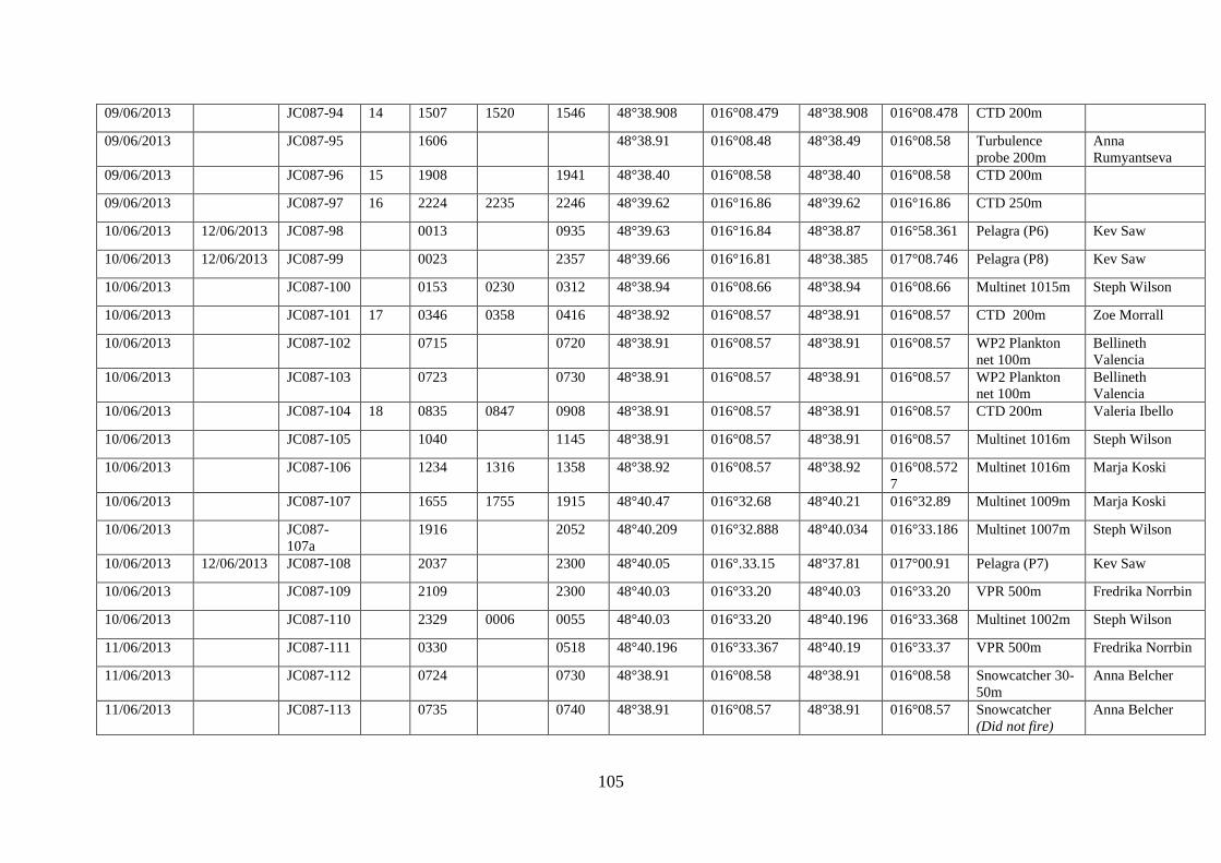
105

09/06/2013 JC087-94 14 1507 1520 1546 48°38.908 016°08.479 48°38.908 016°08.478 CTD 200m

09/06/2013 JC087-95 1606 48°38.91 016°08.48 48°38.49 016°08.58 Turbulence probe 200m

Anna Rumyantseva

09/06/2013 JC087-96 15 1908 1941 48°38.40 016°08.58 48°38.40 016°08.58 CTD 200m

09/06/2013 JC087-97 16 2224 2235 2246 48°39.62 016°16.86 48°39.62 016°16.86 CTD 250m

10/06/2013 12/06/2013 JC087-98 0013 0935 48°39.63 016°16.84 48°38.87 016°58.361 Pelagra (P6) Kev Saw

10/06/2013 12/06/2013 JC087-99 0023 2357 48°39.66 016°16.81 48°38.385 017°08.746 Pelagra (P8) Kev Saw

10/06/2013 JC087-100 0153 0230 0312 48°38.94 016°08.66 48°38.94 016°08.66 Multinet 1015m Steph Wilson

10/06/2013 JC087-101 17 0346 0358 0416 48°38.92 016°08.57 48°38.91 016°08.57 CTD 200m Zoe Morrall

10/06/2013 JC087-102 0715 0720 48°38.91 016°08.57 48°38.91 016°08.57 WP2 Plankton net 100m

Bellineth Valencia

10/06/2013 JC087-103 0723 0730 48°38.91 016°08.57 48°38.91 016°08.57 WP2 Plankton net 100m

Bellineth Valencia

10/06/2013 JC087-104 18 0835 0847 0908 48°38.91 016°08.57 48°38.91 016°08.57 CTD 200m Valeria Ibello

10/06/2013 JC087-105 1040 1145 48°38.91 016°08.57 48°38.91 016°08.57 Multinet 1016m Steph Wilson

10/06/2013 JC087-106 1234 1316 1358 48°38.92 016°08.57 48°38.92 016°08.5727

Multinet 1016m Marja Koski

10/06/2013 JC087-107 1655 1755 1915 48°40.47 016°32.68 48°40.21 016°32.89 Multinet 1009m Marja Koski

10/06/2013 JC087-107a

1916 2052 48°40.209 016°32.888 48°40.034 016°33.186 Multinet 1007m Steph Wilson

10/06/2013 12/06/2013 JC087-108 2037 2300 48°40.05 016°.33.15 48°37.81 017°00.91 Pelagra (P7) Kev Saw

10/06/2013 JC087-109 2109 2300 48°40.03 016°33.20 48°40.03 016°33.20 VPR 500m Fredrika Norrbin

10/06/2013 JC087-110 2329 0006 0055 48°40.03 016°33.20 48°40.196 016°33.368 Multinet 1002m Steph Wilson

11/06/2013 JC087-111 0330 0518 48°40.196 016°33.367 48°40.19 016°33.37 VPR 500m Fredrika Norrbin

11/06/2013 JC087-112 0724 0730 48°38.91 016°08.58 48°38.91 016°08.58 Snowcatcher 30-50m

Anna Belcher

11/06/2013 JC087-113 0735 0740 48°38.91 016°08.57 48°38.91 016°08.57 Snowcatcher (Did not fire)

Anna Belcher

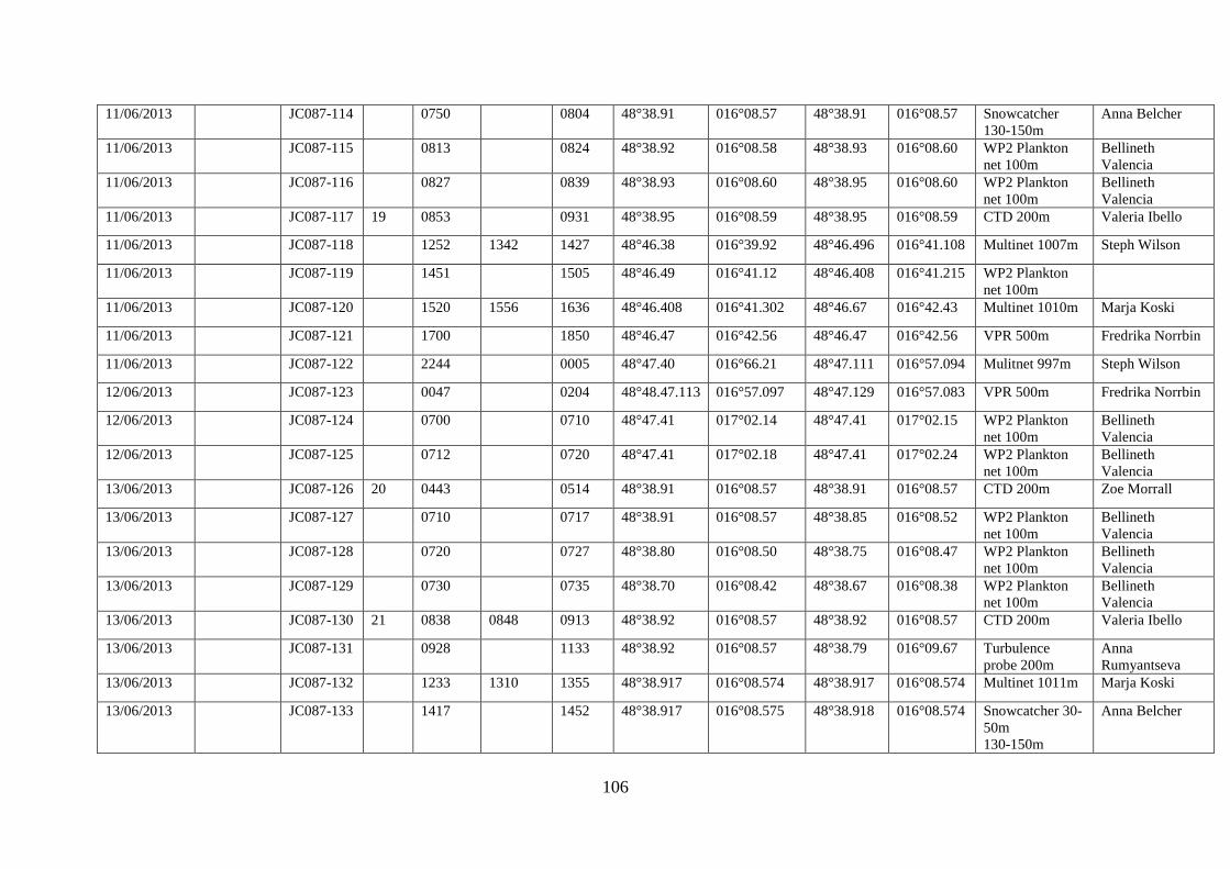
106

11/06/2013 JC087-114 0750 0804 48°38.91 016°08.57 48°38.91 016°08.57 Snowcatcher 130-150m

Anna Belcher

11/06/2013 JC087-115 0813 0824 48°38.92 016°08.58 48°38.93 016°08.60 WP2 Plankton net 100m

Bellineth Valencia

11/06/2013 JC087-116 0827 0839 48°38.93 016°08.60 48°38.95 016°08.60 WP2 Plankton net 100m

Bellineth Valencia

11/06/2013 JC087-117 19 0853 0931 48°38.95 016°08.59 48°38.95 016°08.59 CTD 200m Valeria Ibello

11/06/2013 JC087-118 1252 1342 1427 48°46.38 016°39.92 48°46.496 016°41.108 Multinet 1007m Steph Wilson

11/06/2013 JC087-119 1451 1505 48°46.49 016°41.12 48°46.408 016°41.215 WP2 Plankton net 100m

11/06/2013 JC087-120 1520 1556 1636 48°46.408 016°41.302 48°46.67 016°42.43 Multinet 1010m Marja Koski

11/06/2013 JC087-121 1700 1850 48°46.47 016°42.56 48°46.47 016°42.56 VPR 500m Fredrika Norrbin

11/06/2013 JC087-122 2244 0005 48°47.40 016°66.21 48°47.111 016°57.094 Mulitnet 997m Steph Wilson

12/06/2013 JC087-123 0047 0204 48°48.47.113 016°57.097 48°47.129 016°57.083 VPR 500m Fredrika Norrbin

12/06/2013 JC087-124 0700 0710 48°47.41 017°02.14 48°47.41 017°02.15 WP2 Plankton net 100m

Bellineth Valencia

12/06/2013 JC087-125 0712 0720 48°47.41 017°02.18 48°47.41 017°02.24 WP2 Plankton net 100m

Bellineth Valencia

13/06/2013 JC087-126 20 0443 0514 48°38.91 016°08.57 48°38.91 016°08.57 CTD 200m Zoe Morrall

13/06/2013 JC087-127 0710 0717 48°38.91 016°08.57 48°38.85 016°08.52 WP2 Plankton net 100m

Bellineth Valencia

13/06/2013 JC087-128 0720 0727 48°38.80 016°08.50 48°38.75 016°08.47 WP2 Plankton net 100m

Bellineth Valencia

13/06/2013 JC087-129 0730 0735 48°38.70 016°08.42 48°38.67 016°08.38 WP2 Plankton net 100m

Bellineth Valencia

13/06/2013 JC087-130 21 0838 0848 0913 48°38.92 016°08.57 48°38.92 016°08.57 CTD 200m Valeria Ibello

13/06/2013 JC087-131 0928 1133 48°38.92 016°08.57 48°38.79 016°09.67 Turbulence probe 200m

Anna Rumyantseva

13/06/2013 JC087-132 1233 1310 1355 48°38.917 016°08.574 48°38.917 016°08.574 Multinet 1011m Marja Koski

13/06/2013 JC087-133 1417 1452 48°38.917 016°08.575 48°38.918 016°08.574 Snowcatcher 30-50m 130-150m

Anna Belcher

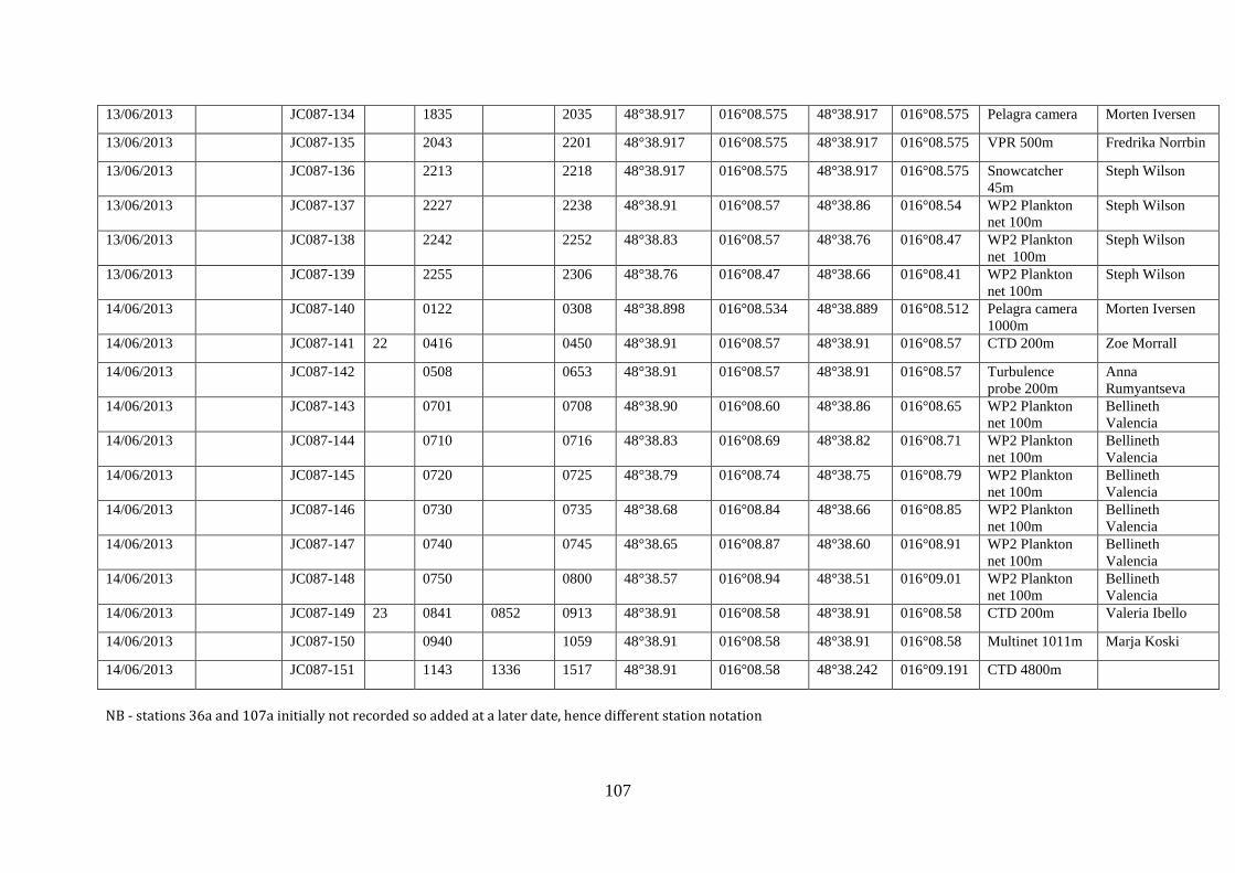
107

NB - stations 36a and 107a initially not recorded so added at a later date, hence different station notation

13/06/2013 JC087-134 1835 2035 48°38.917 016°08.575 48°38.917 016°08.575 Pelagra camera Morten Iversen

13/06/2013 JC087-135 2043 2201 48°38.917 016°08.575 48°38.917 016°08.575 VPR 500m Fredrika Norrbin

13/06/2013 JC087-136 2213 2218 48°38.917 016°08.575 48°38.917 016°08.575 Snowcatcher 45m

Steph Wilson

13/06/2013 JC087-137 2227 2238 48°38.91 016°08.57 48°38.86 016°08.54 WP2 Plankton net 100m

Steph Wilson

13/06/2013 JC087-138 2242 2252 48°38.83 016°08.57 48°38.76 016°08.47 WP2 Plankton net 100m

Steph Wilson

13/06/2013 JC087-139 2255 2306 48°38.76 016°08.47 48°38.66 016°08.41 WP2 Plankton net 100m

Steph Wilson

14/06/2013 JC087-140 0122 0308 48°38.898 016°08.534 48°38.889 016°08.512 Pelagra camera 1000m

Morten Iversen

14/06/2013 JC087-141 22 0416 0450 48°38.91 016°08.57 48°38.91 016°08.57 CTD 200m Zoe Morrall

14/06/2013 JC087-142 0508 0653 48°38.91 016°08.57 48°38.91 016°08.57 Turbulence probe 200m

Anna Rumyantseva

14/06/2013 JC087-143 0701 0708 48°38.90 016°08.60 48°38.86 016°08.65 WP2 Plankton net 100m

Bellineth Valencia

14/06/2013 JC087-144 0710 0716 48°38.83 016°08.69 48°38.82 016°08.71 WP2 Plankton net 100m

Bellineth Valencia

14/06/2013 JC087-145 0720 0725 48°38.79 016°08.74 48°38.75 016°08.79 WP2 Plankton net 100m

Bellineth Valencia

14/06/2013 JC087-146 0730 0735 48°38.68 016°08.84 48°38.66 016°08.85 WP2 Plankton net 100m

Bellineth Valencia

14/06/2013 JC087-147 0740 0745 48°38.65 016°08.87 48°38.60 016°08.91 WP2 Plankton net 100m

Bellineth Valencia

14/06/2013 JC087-148 0750 0800 48°38.57 016°08.94 48°38.51 016°09.01 WP2 Plankton net 100m

Bellineth Valencia

14/06/2013 JC087-149 23 0841 0852 0913 48°38.91 016°08.58 48°38.91 016°08.58 CTD 200m Valeria Ibello

14/06/2013 JC087-150 0940 1059 48°38.91 016°08.58 48°38.91 016°08.58 Multinet 1011m Marja Koski

14/06/2013 JC087-151 1143 1336 1517 48°38.91 016°08.58 48°38.242 016°09.191 CTD 4800m

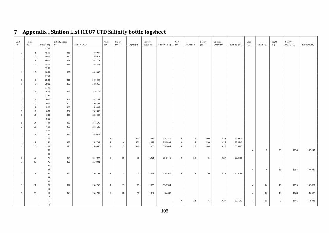
108

7 Appendix I Station List JC087 CTD Salinity bottle logsheet Cast no.

Niskin no. Depth (m)

Salinity bottle no. Salinity (psu)

Cast no.

Niskin no. Depth (m)

Salinity bottle no. Salinity (psu)

Cast no. Niskin no.

Depth (m)

Salinity bottle no. Salinity (psu)

Cast no. Niskin no.

Depth (m)

Salinity bottle no. Salinity (psu)

4799

1 1 4500 356 34.904

1 2 4000 357 34.911

1 3 4000 358 34.9111

1 4 3500 359 34.9225

3250

1 5 3000 360 34.9386

2750

1 6 2500 361 34.9437

1 7 2000 362 34.9262

1750

1 8 1500 363 35.0155

1250

1 9 1000 371 35.4161

1 10 1000 365 35.4161

1 11 800 366 35.2483

1 12 600 367 35.5396

1 13 600 368 35.5406

500

1 14 400 369 35.5108

1 15 400 370 35.5129

300

1 16 250 364 35.5076

200 2 1 200 1028 35.5975 3 1 200 824 35.4759

1 17 150 372 35.5701 2 4 150 1029 35.6491 3 4 150 825 35.4745

1 18 100 373 35.6855 2 7 100 1030 35.6644 3 7 100 826 35.5487

90 4 2 90 1036 35.5141

80

1 19 75 374 35.6894 2 10 75 1031 35.6745 3 10 75 827 35.4705

1 20 75 375 35.6901

70

59 4 4 59 1037 35.4747

1 21 50 376 35.6767 2 13 50 1032 35.6745 3 13 50 828 35.4688

45

30

1 22 25 377 35.6735 2 17 25 1033 35.6784 4 14 25 1039 35.5021

15

1 23 10 378 35.6792 2 20 10 1034 35.682 4 17 10 1040 35.506

7

6 3 22 6 829 35.5002 4 20 6 1041 35.5081

5

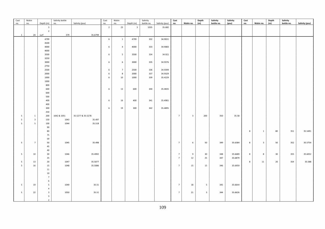
109

Cast no.

Niskin no. Depth (m)

Salinity bottle no. Salinity (psu)

Cast no.

Niskin no. Depth (m)

Salinity bottle no. Salinity (psu)

Cast no. Niskin no.

Depth (m)

Salinity bottle no.

Salinity (psu)

Cast no. Niskin no.

Depth (m)

Salinity bottle no. Salinity (psu)

3 2 23 3 1035 35.682

2

1 24 surf 379 35.6799

4799 6 1 4799 332 34.9031

4500

4000 6 4 4000 333 34.9083

4000

3500 6 5 3500 334 34.921

3250

3000 6 6 3000 335 34.9376

2750

2500 6 7 2500 336 34.9399

2000 6 8 2000 337 34.9329

1000 6 10 1000 339 35.4229

1000

800

600 6 13 600 340 35.4835

600

500

400 6 16 400 341 35.4981

400

300 6 19 300 342 35.4895

250

5 1 200 1042 & 1051 35.5277 & 35.5278 7 3 200 350 35.58

5 3 150 1043 35.497

5 5 100 1044 35.518

90

80 8 1 80 351 35.5491

75

59

5 7 50 1045 35.498 7 6 50 349 35.6384 8 3 50 352 35.5754

45

40

5 10 30 1046 35.4992 7 9 30 348 35.6689 8 8 30 355 35.6052

25 7 12 25 347 35.6879

5 13 20 1047 35.5077 8 11 20 354 35.588

5 16 15 1048 35.5086 7 15 15 346 35.6959

11

10

7

6

5 19 5 1049 35.51 7 18 5 345 35.6644

4

5 22 3 1050 35.51 7 21 3 344 35.6626

3

2

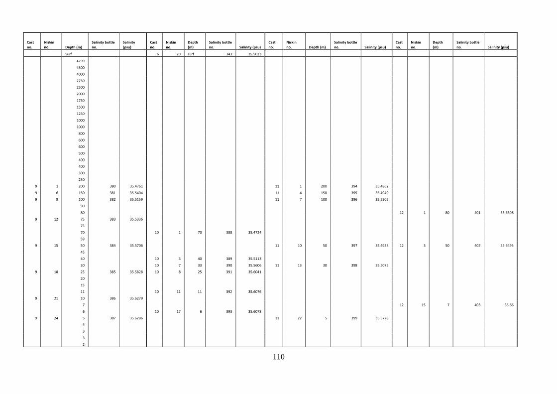
110

Cast no.

Niskin no. Depth (m)

Salinity bottle no.

Salinity (psu)

Cast no.

Niskin no.

Depth (m)

Salinity bottle no. Salinity (psu)

Cast no.

Niskin no. Depth (m)

Salinity bottle no. Salinity (psu)

Cast no.

Niskin no.

Depth (m)

Salinity bottle no. Salinity (psu)

Surf 6 20 surf 343 35.5023

4799

4500

4000

2750

2500

2000

1750

1500

1250

1000

1000

800

600

600

500

400

400

300

250

9 1 200 380 35.4761 11 1 200 394 35.4862

9 6 150 381 35.5404 11 4 150 395 35.4949

9 9 100 382 35.5159 11 7 100 396 35.5205

90

80 12 1 80 401 35.6508

9 12 75 383 35.5336

75

70 10 1 70 388 35.4724

59

9 15 50 384 35.5706 11 10 50 397 35.4933 12 3 50 402 35.6495

45

40 10 3 40 389 35.5113

30 10 7 33 390 35.5606 11 13 30 398 35.5075

9 18 25 385 35.5828 10 8 25 391 35.6041

20

15

11 10 11 11 392 35.6076

9 21 10 386 35.6279

7 12 15 7 403 35.66

6 10 17 6 393 35.6078

9 24 5 387 35.6286 11 22 5 399 35.5728

4

3

3

2

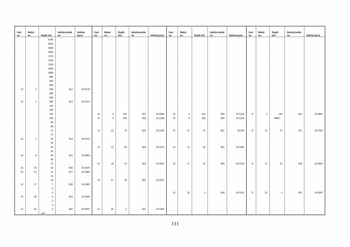
111

Cast no.

Niskin no. Depth (m)

Salinity bottle no.

Salinity (psu)

Cast no.

Niskin no.

Depth (m)

Salinity bottle no. Salinity (psu)

Cast no.

Niskin no. Depth (m)

Salinity bottle no. Salinity (psu)

Cast no.

Niskin no.

Depth (m)

Salinity bottle no. Salinity (psu)

4799

4500

4000

2000

1750

1500

1250

1000

1000

800

600

600

13 1 500 812 35.3578

400

400

13 2 300 813 35.4721

250

200

150 14 6 150 827 35.4926 15 5 150 829 35.5118 17 5 150 356 35.4891

100 14 9 100 826 35.5198 15 8 100 830 35.5334 #REF!

90

80

75 14 12 75 825 35.5185 15 12 75 831 35.554 17 11 75 357 35.5505

75

13 3 70 814 35.5975

59

50 14 15 50 824 35.5374 15 15 50 832 35.5284

45

13 8 40 815 35.6053

30

25 14 18 25 823 35.5814 15 17 25 833 35.5234 17 17 25 358 35.6462

13 10 20 816 35.5874

13 13 15 817 35.5983

11

10 14 21 10 822 35.5597

13 17 7 818 35.5945

6

5 15 23 5 834 35.5232 17 23 5 359 35.6267

13 20 4 819 35.5945

3

3

13 23 2 820 35.5937 14 24 2 821 35.5492

surf

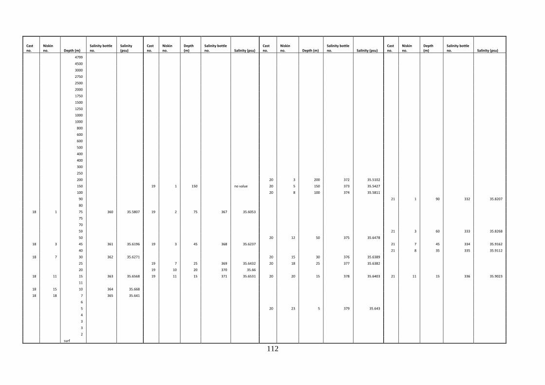
112

Cast no.

Niskin no. Depth (m)

Salinity bottle no.

Salinity (psu)

Cast no.

Niskin no.

Depth (m)

Salinity bottle no. Salinity (psu)

Cast no.

Niskin no. Depth (m)

Salinity bottle no. Salinity (psu)

Cast no.

Niskin no.

Depth (m)

Salinity bottle no. Salinity (psu)

4799

4500

3000

2750

2500

2000

1750

1500

1250

1000

1000

800

600

600

500

400

400

300

250

200 20 3 200 372 35.5102

150 19 1 150 no value 20 5 150 373 35.5427

100 20 8 100 374 35.5811

90 21 1 90 332 35.8207

80

18 1 75 360 35.5807 19 2 75 367 35.6053

75

70

59 21 3 60 333 35.8268

50 20 12 50 375 35.6478

18 3 45 361 35.6196 19 3 45 368 35.6237 21 7 45 334 35.9162

40 21 8 35 335 35.9112

18 7 30 362 35.6271 20 15 30 376 35.6389

25 19 7 25 369 35.6432 20 18 25 377 35.6382

20 19 10 20 370 35.66

18 11 15 363 35.6568 19 11 15 371 35.6531 20 20 15 378 35.6403 21 11 15 336 35.9023

11

18 15 10 364 35.668

18 18 7 365 35.641

6

5 20 23 5 379 35.643

4

3

3

2

surf

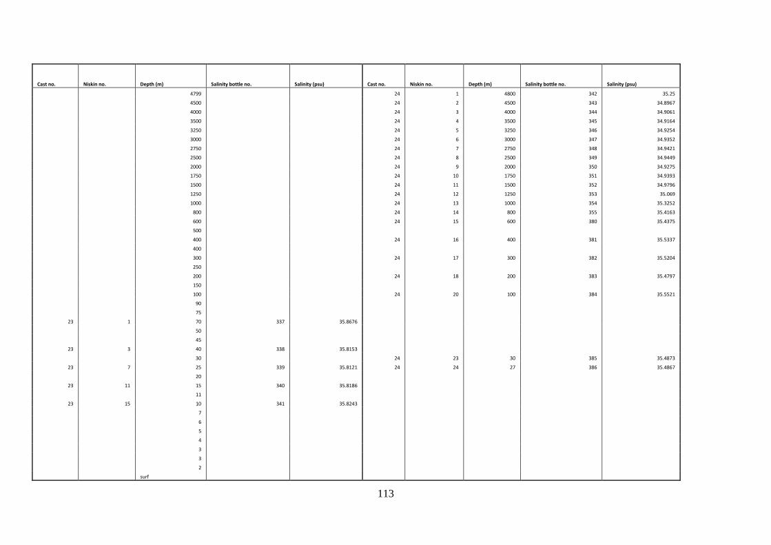
113

Cast no. Niskin no. Depth (m) Salinity bottle no. Salinity (psu) Cast no. Niskin no. Depth (m) Salinity bottle no. Salinity (psu)

4799 24 1 4800 342 35.25

4500 24 2 4500 343 34.8967

4000 24 3 4000 344 34.9061

3500 24 4 3500 345 34.9164

3250 24 5 3250 346 34.9254

3000 24 6 3000 347 34.9352

2750 24 7 2750 348 34.9421

2500 24 8 2500 349 34.9449

2000 24 9 2000 350 34.9275

1750 24 10 1750 351 34.9393

1500 24 11 1500 352 34.9796

1250 24 12 1250 353 35.069

1000 24 13 1000 354 35.3252

800 24 14 800 355 35.4163

600 24 15 600 380 35.4375

500

400 24 16 400 381 35.5337

400

300 24 17 300 382 35.5204

250

200 24 18 200 383 35.4797

150

100 24 20 100 384 35.5521

90

75

23 1 70 337 35.8676

50

45

23 3 40 338 35.8153

30 24 23 30 385 35.4873

23 7 25 339 35.8121 24 24 27 386 35.4867

20

23 11 15 340 35.8186

11

23 15 10 341 35.8243

7

6

5

4

3

3

2

surf

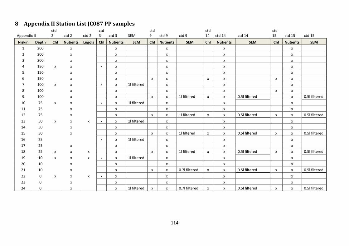
114

8 Appendix II Station List JC087 PP samples

Appendix II ctd 2 ctd 2 ctd 2

ctd 3 ctd 3 SEM

ctd 9 ctd 9 ctd 9

ctd 14 ctd 14 ctd 14

ctd 15 ctd 15 ctd 15

Niskin Depth Chl Nutients Lugols Chl Nutients SEM Chl Nutients SEM Chl Nutients SEM Chl Nutients SEM 1 200 x x x x x 2 200

x x x x x

3 200

x x x x x 4 150 x x x x x x x 5 150

x x x x x

6 150

x x x x x x x x 7 100 x x x x 1l filtered x x x 8 100

x x x x x x

9 100

x x x x 1l filtered x x 0.5l filtered x 0.5l filtered 10 75 x x x x 1l filtered x x x 11 75

x x x x x

12 75

x x x x 1l filtered x x 0.5l filtered x x 0.5l filtered 13 50 x x x x x 1l filtered x x x 14 50

x x x x x

15 50

x x x x 1l filtered x x 0.5l filtered x x 0.5l filtered 16 25

x x 1l filtered x x x

17 25

x x x x x 18 25 x x x x x x 1l filtered x x 0.5l filtered x x 0.5l filtered 19 10 x x x x x 1l filtered x x x 20 10

x x x x x

21 10

x x x x 0.7l filtered x x 0.5l filtered x x 0.5l filtered 22 0 x x x x x x x x 23 0

x x x x x

24 0 x x 1l filtered x x 0.7l filtered x x 0.5l filtered x x 0.5l filtered