NaSCoIT 2018 Published Papers 9 th National Students’ Conference on Information Technology

Welcome message from author
This document is posted to help you gain knowledge. Please leave a comment to let me know what you think about it! Share it to your friends and learn new things together.
Transcript

NaSCoIT
2018
Published
Papers
9th National Students’ Conference on
Information Technology


Intrusion Detection with Feature Selection and Dimension
Reduction using WEKA
Anku Jaiswal Department of Electronics and
Computer Engineering
Advanced College of
Engineering and Management
Lalitpur, Nepal
Dr. Subarna Shakya Department of Electronics and
Computer Engineering
Institute of Engineering
Tribhuban University
Prakash Chandra Prasad CEO, Infography Technologies
Pvt.Ltd
Lalitpur,Nepal
Narayan KC M.E. Computer Engineering, 2009, NCIT
Department of Electronics and Computer Engineering
Advanced College of Engineering and Management
Lalitpur, Nepal
Raisha Shrestha B.E. Computer Engineering 2017
Advanced College of Engineering and Management
Lalitpur, Nepal
Abstract— As Internet is growing with a high
speed, there are large number security audit data
and complex intrusion behavior which makes the
current intrusion system inefficient. Intrusion
detection using data mining and machine learning
can be one of the solutions to this problem. For
this we can build intrusion detection system using
machine learning algorithm. One of the machine
learning and data mining tools that can be used
for this purpose is WEKA which uses various
algorithms. With this tool we can develop a model
using various algorithms which can distinguish
normal and malicious traffic and also we can
analyze which algorithm gives accurate result. For
a model to be created a dataset is given with large
number of features and all the features are not
that important. Feature selection helps in reducing
computational time. We should be able to select
various attributes which helps in developing an
effective model in WEKA. The same model can be
trained and used for other test data. The analysis
is performed with a traffic data called VPN-
nonVPN dataset from ISCX which consist of 14
different traffic categories. This dataset consist of
two class called VPN and non-VPN, and the model
can classify correctly whether the traffic is coming
from VPN or a non-VPN. This paper mainly deals
with creation of model for intrusion detection
using WEKA and also shows how the accuracy
can be increased by feature selection and
dimension reduction.
Keywords— WEKA, Machine Learning, Data
Mining, Classifier, Data Collection, Feature
Selection, ROC curve
1. Introduction Data mining is defined as process of extracting useful
information from a large dataset. It involves
removing unwanted features, cleaning the data and
making it suitable for using in a model. Machine
learning is a method to train a machine so that it can
be used for intrusion detection without human
intervention. WEKA tool is use to create a model and
train it to perform in an effective manner for various
dataset. While downloading many datasets it may be
in various formats such as pcap, csv. Converting the
data into a format readable by a model using a tool is
one of the major tasks. Intelligent intrusion detection
system can be built only if we have an effective
dataset [3].A data has a number of features and not all
the features are useful, hence selecting only the
needed feature is another task. Most of the paper has
used NSL-KDD dataset for the purpose of intrusion
detection. But this paper deals with data downloaded
from ICSX which has been collected from VPN and
non-VPN. The model created will classify whether
the traffic is coming from a VPN or not. First section of paper deals with collection of dataset
from various sites which can be in the form of arff or
csv format.
Collecting a proper data can be a tedious task. This
section discuss about the data used in this paper and
also the process of collecting the data. In third section we deal with feature selection and reduction of the traffic data which can be done by
using two methods: filter and wrapper. It is observed
that the reduced features affect the accuracy of various models. In fourth section we discuss about performance of
different algorithm and classifier which comes under
rules, Bayes, trees, lazy using a particular dataset. For the same dataset, different algorithms produce
different result.

In fifth section data is divided into test and train data
using WEKA. It shows how the accuracy of a model differs using a train data and again reevaluating the
same model for test data.
2. Related Work Effective data can be collected for analysis of a
model which consist of real world traffic and is also
known as ISCX VPN- nonVPN traffic
dataset[1][2].Weka is one of the strongest tool which
is collection of machine learning algorithm for data
mining task [3]. Weka consists of a number of tools
for data pre-processing, association rules and
visualization. It is also used for developing new
machine learning algorithm. Selecting important
feature on the basis of rough set based feature
selection approach have led to a simplification of the
problem, faster and more accurate detection rates [4].
Feature selection is a tough task than feature
extraction. Selecting correct and required features
using two methods called filter and wrapper method
can increase the accuracy of a classifier [5][6]. Weka
tool consist of a number of machine learning
algorithms which can be classified such as: i) Bayes:
Naïve Bayes and Bayes Net ii) Tree: j48, NBTree iii)
Rule: Decision Tree, jRip, oneR iv)Lazy: jBk. All
these classifiers have their own advantages and their
accuracy depends on the type of dataset [7] [8] [9].
Different models can be built and classifier accuracy
can be compared based on the same dataset. This is
the accuracy of the model when we take training data
and when we use the built model for test data differs.
The dataset can be divided into train and test dataset
to build a more efficient model [6][10].
About the dataset
The dataset used in this paper is real world traffic
present is ISCX (Information Security Center of Excellence). It consists of network traffic (VPN and
non- VPN dataset). The steps for generation of dataset by ISCX is given below [1] [2].
A set of tasks were defined to generate a representative dataset of real-world traffic in ISCX (Assuring that the dataset was rich enough in diversity and quantity).
Accounts were created for users Alice and Bob in order to use services like Skype, Facebook, etc.
A regular session and a session over VPN were captured, which had a total of 14 traffic categories: VOIP, VPN-VOIP, P2P, VPN-P2P, etc.
Different types of traffic generated and their contents are:
Table 1: Description of Dataset
TRAFFIC CONTENT
Web Browsing Firefox and Chrome
Email SMPTS, POP3S and IMAPS
Chat ICQ, AIM, Skype , Facebook and
Hangouts
Streaming Video and YouTube
File Transfer Skype, FTPS and SFTP using
Filezilla and an external service
VoIP Facebook, Skype and Hangouts
voice calls (1h du ration)
P2P uTorrent and Transmission (Bit
torrent)
The traffic was captured using WireShark and Tcpdump, generating a total amount of 28GB of data. For the VPN, an external VPN service provider was used and connected to it using OpenVPN (UDP mode).
3. Feature selection and dimension
reduction Machine Learning and Data Mining has been used to
improve the accuracy of classifier. A dataset consist
of large number of features and not all the features
are important. Selection of feature and reducing
unwanted features is one of the most important
factors to increase the efficiency of the classifier.
There are two methods for feature selection and
reduction: wrapper method and filter method. Both of
them are discussed below: Wrapper Method: In wrapper method we use subset
evaluator to create all possible subset from your
feature vector. Then it will use a classification
algorithm to induce classifier from the features in a
subset. It will consider the subset of features with the
classification algorithm performs the best. For
example we have 10 features, the evaluator try to find
subset with those 10 features.
1st attribute: 3 features
2nd
attribute: 3 features 3
rd attribute: 4 features
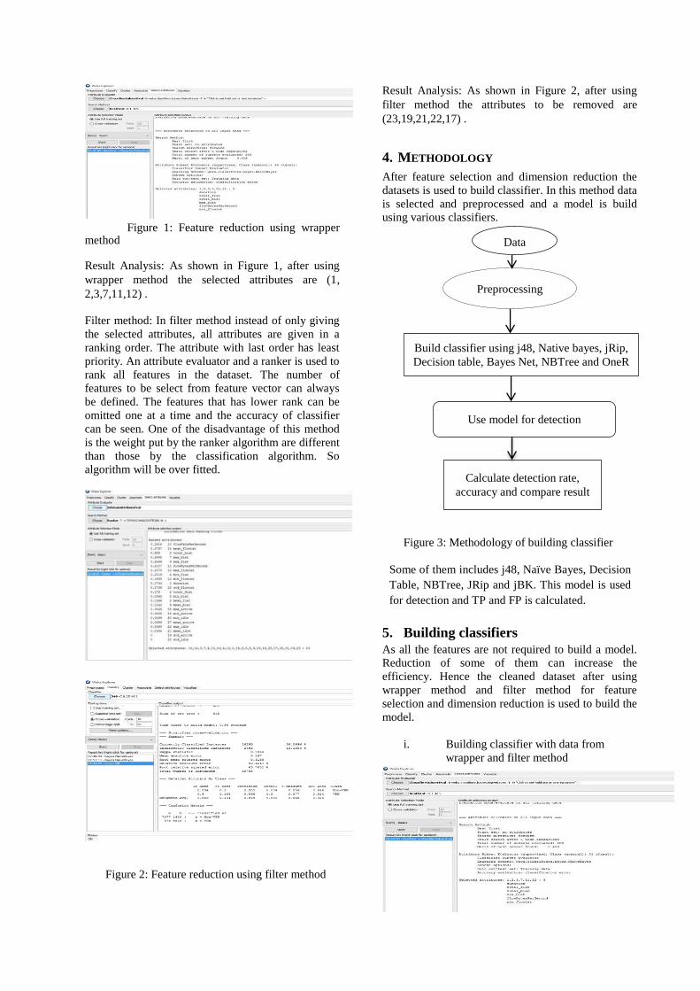
Figure 1: Feature reduction using wrapper
method
Result Analysis: As shown in Figure 1, after using
wrapper method the selected attributes are (1,
2,3,7,11,12) .
Filter method: In filter method instead of only giving
the selected attributes, all attributes are given in a
ranking order. The attribute with last order has least
priority. An attribute evaluator and a ranker is used to
rank all features in the dataset. The number of
features to be select from feature vector can always
be defined. The features that has lower rank can be
omitted one at a time and the accuracy of classifier
can be seen. One of the disadvantage of this method
is the weight put by the ranker algorithm are different
than those by the classification algorithm. So
algorithm will be over fitted.
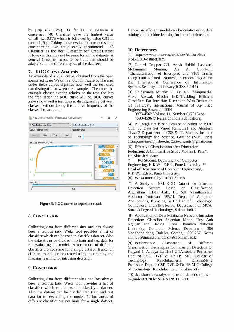
Figure 2: Feature reduction using filter method
Result Analysis: As shown in Figure 2, after using
filter method the attributes to be removed are
(23,19,21,22,17) .
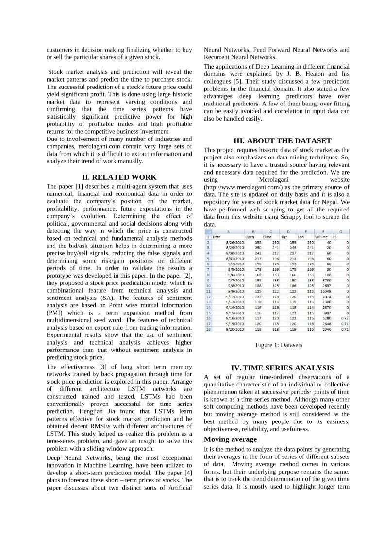
4. METHODOLOGY
After feature selection and dimension reduction the
datasets is used to build classifier. In this method data
is selected and preprocessed and a model is build
using various classifiers.
Figure 3: Methodology of building classifier
Some of them includes j48, Naïve Bayes, Decision
Table, NBTree, JRip and jBK. This model is used
for detection and TP and FP is calculated.
5. Building classifiers
As all the features are not required to build a model.
Reduction of some of them can increase the
efficiency. Hence the cleaned dataset after using
wrapper method and filter method for feature
selection and dimension reduction is used to build the
model.
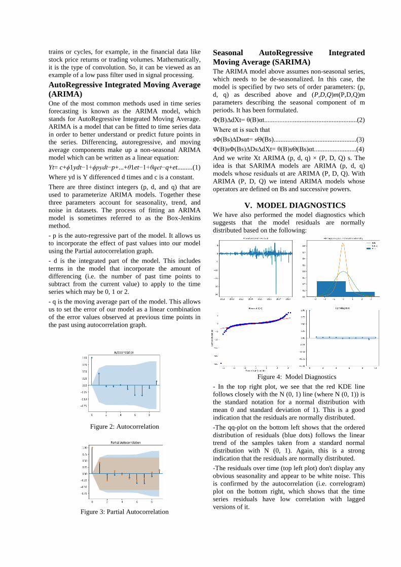
i. Building classifier with data from
wrapper and filter method
Data
Preprocessing
Build classifier using j48, Native bayes, jRip,
Decision table, Bayes Net, NBTree and OneR
Use model for detection
Calculate detection rate,
accuracy and compare result

Figure 4: Building classifier using j48 Figure 4 shows the model created after using the feature selected data using wrapper method.
Table 2: Accuracy of classifier after feature
reduction with wrapper method
Classifier Accuracy (%) Attributes
Naïve Bayes 53.22 With all attributes
Naïve Bayes 55.5017 With selected
attributes
J48 86.8696 With all
attributes
J48 89.726 With selected attributes
Result Analysis: Table 2 shows the accuracy of
classifiers after feature reduction using wrapper
method. As seen the accuracy of classifier is
increased in case of both Naïve Bayes and J48 to
55.5017 and 89.726 after feature reduction.
Table 3: Accuracy of classifier after feature
reduction
Classi
fier
Attribute
removed Correctly classified
instance
J48 23 89.7217
J48 23,19 89.743
J48 23,19,21 89.7537
J48 23,19,21,22 89.7057 over fitted
J48 23,19,21,22,1
7 89.7057
Result Analysis: Table 3 shows the accuracy of
classifiers after feature reduction using filter method.
As seen the accuracy of classifier is increased in case
J48 to 89.7057 after feature reduction.
6. Result The values for the evaluation measures can be
different for the different data sets used and
accordingly the algorithms may perform in the
different way for the different datasets.
Table 4: Comparison of various classifiers
Classif
ier TP FP Correctly Incorrectly Class
classified classified
instance instance Bayes 0.728 0.126 80.387 19.613 Non-
Net 0.874 0.272 VPN VPN
Naïve 0.045 0.022 53.22 46.78 Non- Bayes 0.978 0.955 VPN
VPN
J48 0.876 0.084 89.727 10.273 Non- 0.916 0.124 VPN VPN
NBTre
e 0.748 0.118 81.7624 18.2576 Non- 0.882 0.252 VPN
VPN
Decisi
on 0.764 0.133 81.9864 18.0136 Non- table 0.867 0.231 VPN
VPN
JRip 0.81 0.067 87.392 12.608 Non-
0.933 0.19 VPN
VPN
Table 4 shows that for the same real VPN-nonVPN dataset, different algorithms works in a different ways. J48 classifier shows the highest percent of correctly classified Instances (89.727%) after feature selection and dimension reduction which is followed
by jRip (87.392%). As far as TP measure is concerned, j48 Classifier gave the highest value of all i.e. 0.876 which is followed by value 0.81 in case of jRip. Taking these evaluation measures into consideration, we could easily recommend j48 Classifier as the best Classifier for Credit Dataset . However this may not be same for all the datasets. A general Classifier needs to be built that should be adaptable to the different types of the datasets. 7. ROC Curve Analysis An example of a ROC curve, obtained from the open source software Weka, is shown in Figure 5. The area under these curves signifies how well the test used can distinguish between the examples. The more the example classes overlap relative to the test, the less the area under the ROC curve will be. ROC curves shows how well a test does at distinguishing between classes without taking the relative frequency of the classes into account.
Figure 5: ROC curve to represent result
8. CONCLUSION
Collecting data from different sites and has always been a tedious task. Weka tool provides a list of
classifier which can be used to classify a dataset. Also the dataset can be divided into train and test data for
re- evaluating the model. Performances of different
classifier are not same for a single dataset. Hence, an efficient model can be created using data mining and
machine learning for intrusion detection.
9. CONCLUSION
Collecting data from different sites and has always been a tedious task. Weka tool provides a list of classifier which can be used to classify a dataset. Also the dataset can be divided into train and test data for re- evaluating the model. Performances of different classifier are not same for a single dataset.
Hence, an efficient model can be created using data mining and machine learning for intrusion detection.
10. References [1] http://www.unb.ca/research/iscx/dataset/iscx-NSL-KDD-dataset.html [2] Gerard Drapper Gil, Arash Habibi Lashkari, Mohammad Mamun, Ali A. Ghorbani, "Characterization of Encrypted and VPN Traffic Using Time-Related Features", In Proceedings of the 2nd International Conference on Information Systems Security and Privacy(ICISSP 2016) [3] Chidananda Murthy P., Dr A.S. Manjunatha, Anku Jaiswal, Madhu B.R.“Building Efficient Classifiers For Intrusion D etection With Reduction Of Features”, International Journal of Ap plied Engineering Research ISSN
0973-4562 Volume 11, Number 6 (2016) pp. 4590-4596 © Research India Publications.
[4] A Rough Set Based Feature Selection on KDD CUP 99 Data Set Vinod Rampure1 and Akhilesh Tiwari2 Department of CSE & IT, Madhav Institute of Technology and Science, Gwalior (M.P), India [email protected], [email protected] [5] Effective Classification after Dimension
Reduction: A Comparative Study Mohini D Patil*,
Dr. Shirish S. Sane * PG Student, Department of Computer Engineering, K.K.W.I.E.E.R, Pune University. ** Head of Department of Computer Engineering, K.K.W.I.E.E.R, Pune University. [6] Weka tutorial by Rushdi Shams [7] A Study on NSL-KDD Dataset for Intrusion Detection System Based on Classification Algorithms L.Dhanabal1, Dr. S.P. Shantharajah2 Assistant Professor [SRG], Dept. of Computer Applications, Kumaraguru College of Technology, Coimbatore, India1Professor, Department of MCA, Sona College of Technology, Salem, India2 [8] Application of Data Mining to Network Intrusion Detection: Classifier Selection Model Huy Anh Nguyen and Deokjai Choi Chonnam National University, Computer Science Department, 300 Yongbong-dong, Buk-ku, Gwangju 500-757, Korea [email protected], [email protected] [9] Performance Assessment of Different Classification Techniques for Intrusion Detection G. Kalyani 1, A. Jaya Lakshmi 2 1Associate Professor, Dept of CSE, DVR & Dr HS MIC College of Technology, Kanchikacherla, Krishna(dt),2 Professor, Dept of CSE DVR & Dr HS MIC College of Technology, Kanchikacherla, Krishna (dt),. [10] decision-tree-analysis-intrusion-detection-how-
to-guide-33678 by SANS INSTITUTE


Stock Market Forecast Using Time Series Analysis
Prakash Chandra Prasad CEO, Infography Technologies Pvt.Ltd
Lalitpur,Nepal
Lujina Maharjan Department of Electronics and Computer Engineering Advanced College of Engineering and Management
Lalitpur, Nepal
Anku Jaiswal Department of Electronics and Computer Engineering
Advanced College of Engineering and Management Lalitpur, Nepal
Abstract Stock market, one of the financially
volatile markets has attracted thousands of
investors’ hearts since its existence. The profit and
risk of it has great beauty and everyone wants to get
some benefits from it, so the stock price forecasting
has always been a popular field of study in the area
of financial data mining. Many methods like
technical analysis, fundamental analysis, statistical
analysis etc. are being used to predict the stock
price in the share market but no one method has
proved to be consistent forecasting tool. This paper
contributes to the field of Time Series Analysis,
which aims to forecast the stock market price using
previous recorded stock prices. It discusses about
how the Moving Average method can be used to
identify the unknown and hidden patterns in share
market data considering SARIMA as noble method.
The proposed system consists of building and
training the models using the past data of the
selected stock and the results obtained from the
model for comparing with the real data so as to
ascertain the accuracy of the model. This result
contributes to the development of more robust
forecasting for the purpose of qualitative and
quantitative information.
Dipinti Manandhar Department of Electronics and Computer Engineering
Advanced College of Engineering and Management
Lalitpur, Nepal
Lisa Rajkarnikar Department of Electronics and Computer Engineering
Advanced College of Engineering and Management Lalitpur, Nepal
regarding the stock prices. In addition, it enables the
users to make the smart decision for stock trading.
Keywords Moving Average, ARIMA , SARIMA,
Time series analysis, Mero lagani, Stock market
I. INTRODUCTION Prediction of stock market data is known as a prominent
issue for stock traders. Stock market data has a highly
dynamic property due to a conflicting extent of
influential factors
A stock market is a public market for the trading of
company stock and derivatives at an agreed price. Stock
market is the important part of economy of the country
and plays a vital role in the growth of the country. Both
investors and industry are involved in stock market and
wants to know whether some stock will rise or fall over
a period of time. It is based on the concept of demand
and supply. If the demand for a company‟s stock is
higher, then the company share price increases and if
the demand for company‟s stock is less then the
company share price decreases. Indeed, forecasting the
trend of stock market rise or fall incident need to be
focused because the obtained result can be utilized for
customers in decision making finalizing whether to buy
or sell the particular shares of a given stock.
Stock market analysis and prediction will reveal the
market patterns and predict the time to purchase stock.
The successful prediction of a stock's future price could
yield significant profit. This is done using large historic
market data to represent varying conditions and
confirming that the time series patterns have
statistically significant predictive power for high
probability of profitable trades and high profitable
returns for the competitive business investment
Due to involvement of many number of industries and
companies, merolagani.com contain very large sets of
data from which it is difficult to extract information and
analyze their trend of work manually.
II. RELATED WORK
The paper [1] describes a multi-agent system that uses
numerical, financial and economical data in order to
evaluate the company‟s position on the market,
profitability, performance, future expectations in the
company‟s evolution. Determining the effect of
political, governmental and social decisions along with
detecting the way in which the price is constructed
based on technical and fundamental analysis methods
and the bid/ask situation helps in determining a more
precise buy/sell signals, reducing the false signals and
determining some risk/gain positions on different
periods of time. In order to validate the results a
prototype was developed in this paper. In the paper [2],
they proposed a stock price predication model which is
combinational feature from technical analysis and
sentiment analysis (SA). The features of sentiment
analysis are based on Point wise mutual information
(PMI) which is a term expansion method from
multidimensional seed word. The features of technical
analysis based on expert rule from trading information.
Experimental results show that the use of sentiment
analysis and technical analysis achieves higher
performance than that without sentiment analysis in
predicting stock price.
The effectiveness [3] of long short term memory
networks trained by back propagation through time for
stock price prediction is explored in this paper. Arrange
of different architecture LSTM networks are
constructed trained and tested. LSTMs had been
conventionally proven successful for time series
prediction. Hengjian Jia found that LSTMs learn
patterns effective for stock market prediction and he
obtained decent RMSEs with different architectures of
LSTM. This study helped us realize this problem as a
time-series problem, and gave an insight to solve this
problem with a sliding window approach.
Deep Neural Networks, being the most exceptional
innovation in Machine Learning, have been utilized to
develop a short-term prediction model. The paper [4]
plans to forecast these short – term prices of stocks. The
paper discusses about two distinct sorts of Artificial
Neural Networks, Feed Forward Neural Networks and
Recurrent Neural Networks.
The applications of Deep Learning in different financial
domains were explained by J. B. Heaton and his
colleagues [5]. Their study discussed a few prediction
problems in the financial domain. It also stated a few
advantages deep learning predictors have over
traditional predictors. A few of them being, over fitting
can be easily avoided and correlation in input data can
also be handled easily.
III. ABOUT THE DATASET This project requires historic data of stock market as the
project also emphasizes on data mining techniques. So,
it is necessary to have a trusted source having relevant
and necessary data required for the prediction. We are
using Merolagani website
(http://www.merolagani.com/) as the primary source of
data. The site is updated on daily basis and it is also a
repository for years of stock market data for Nepal. We
have performed web scraping to get all the required
data from this website using Scrappy tool to scrape the
data.
Figure 1: Datasets
IV. TIME SERIES ANALYSIS A set of regular time-ordered observations of a
quantitative characteristic of an individual or collective
phenomenon taken at successive periods/ points of time
is known as a time series method. Although many other
soft computing methods have been developed recently
but moving average method is still considered as the
best method by many people due to its easiness,
objectiveness, reliability, and usefulness.
Moving average
It is the method to analyze the data points by generating
their averages in the form of series of different subsets
of data. Moving average method comes in various
forms, but their underlying purpose remains the same,
that is to track the trend determination of the given time
series data. It is mostly used to highlight longer term
trains or cycles, for example, in the financial data like
stock price returns or trading volumes. Mathematically,
it is the type of convolution. So, it can be viewed as an
example of a low pass filter used in signal processing.
AutoRegressive Integrated Moving Average
(ARIMA) One of the most common methods used in time series
forecasting is known as the ARIMA model, which
stands for AutoRegressive Integrated Moving Average.
ARIMA is a model that can be fitted to time series data
in order to better understand or predict future points in
the series. Differencing, autoregressive, and moving
average components make up a non-seasonal ARIMA
model which can be written as a linear equation:
Yt= c+ϕ1ydt−1+ϕpydt−p+...+θ1et−1+θqet−q+et.........(1)
Where yd is Y differenced d times and c is a constant.
There are three distinct integers (p, d, and q) that are
used to parameterize ARIMA models. Together these
three parameters account for seasonality, trend, and
noise in datasets. The process of fitting an ARIMA
model is sometimes referred to as the Box-Jenkins
method.
- p is the auto-regressive part of the model. It allows us
to incorporate the effect of past values into our model
using the Partial autocorrelation graph.
- d is the integrated part of the model. This includes
terms in the model that incorporate the amount of
differencing (i.e. the number of past time points to
subtract from the current value) to apply to the time
series which may be 0, 1 or 2.
- q is the moving average part of the model. This allows
us to set the error of our model as a linear combination
of the error values observed at previous time points in
the past using autocorrelation graph.
Figure 2: Autocorrelation
Figure 3: Partial Autocorrelation
Seasonal AutoRegressive Integrated
Moving Average (SARIMA) The ARIMA model above assumes non-seasonal series,
which needs to be de-seasonalized. In this case, the
model is specified by two sets of order parameters: (p,
d, q) as described above and (P,D,Q)m(P,D,Q)m
parameters describing the seasonal component of m
periods. It has been formulated.
Φ(B)∆dXt= θ(B)αt.......................................................(2)
Where αt is such that
sΦ(Bs)∆Dsαt= sΘ(Bs).................................................(3)
Φ(B)sΦ(Bs)∆Ds∆dXt= θ(B)sΘ(Bs)αt.........................(4)
And we write Xt ARIMA (p, d, q) × (P, D, Q) s. The
idea is that SARIMA models are ARIMA (p, d, q)
models whose residuals αt are ARIMA (P, D, Q). With
ARIMA (P, D, Q) we intend ARIMA models whose
operators are defined on Bs and successive powers.
V. MODEL DIAGNOSTICS We have also performed the model diagnostics which
suggests that the model residuals are normally
distributed based on the following:
Figure 4: Model Diagnostics
- In the top right plot, we see that the red KDE line
follows closely with the N (0, 1) line (where N (0, 1)) is
the standard notation for a normal distribution with
mean 0 and standard deviation of 1). This is a good
indication that the residuals are normally distributed.
-The qq-plot on the bottom left shows that the ordered
distribution of residuals (blue dots) follows the linear
trend of the samples taken from a standard normal
distribution with N (0, 1). Again, this is a strong
indication that the residuals are normally distributed.
-The residuals over time (top left plot) don't display any
obvious seasonality and appear to be white noise. This
is confirmed by the autocorrelation (i.e. correlogram)
plot on the bottom right, which shows that the time
series residuals have low correlation with lagged
versions of it.
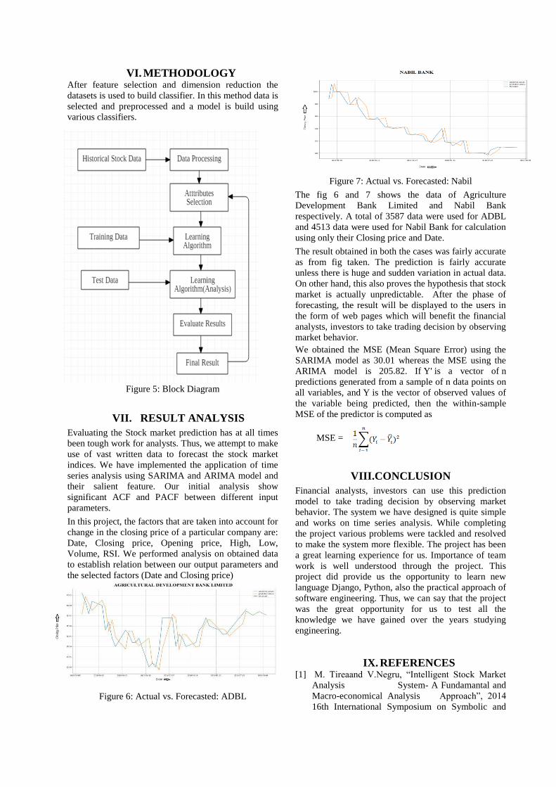
VI. METHODOLOGY After feature selection and dimension reduction the
datasets is used to build classifier. In this method data is
selected and preprocessed and a model is build using
various classifiers.
Figure 5: Block Diagram
VII. RESULT ANALYSIS
Evaluating the Stock market prediction has at all times
been tough work for analysts. Thus, we attempt to make
use of vast written data to forecast the stock market
indices. We have implemented the application of time
series analysis using SARIMA and ARIMA model and
their salient feature. Our initial analysis show
significant ACF and PACF between different input
parameters.
In this project, the factors that are taken into account for
change in the closing price of a particular company are:
Date, Closing price, Opening price, High, Low,
Volume, RSI. We performed analysis on obtained data
to establish relation between our output parameters and
the selected factors (Date and Closing price)
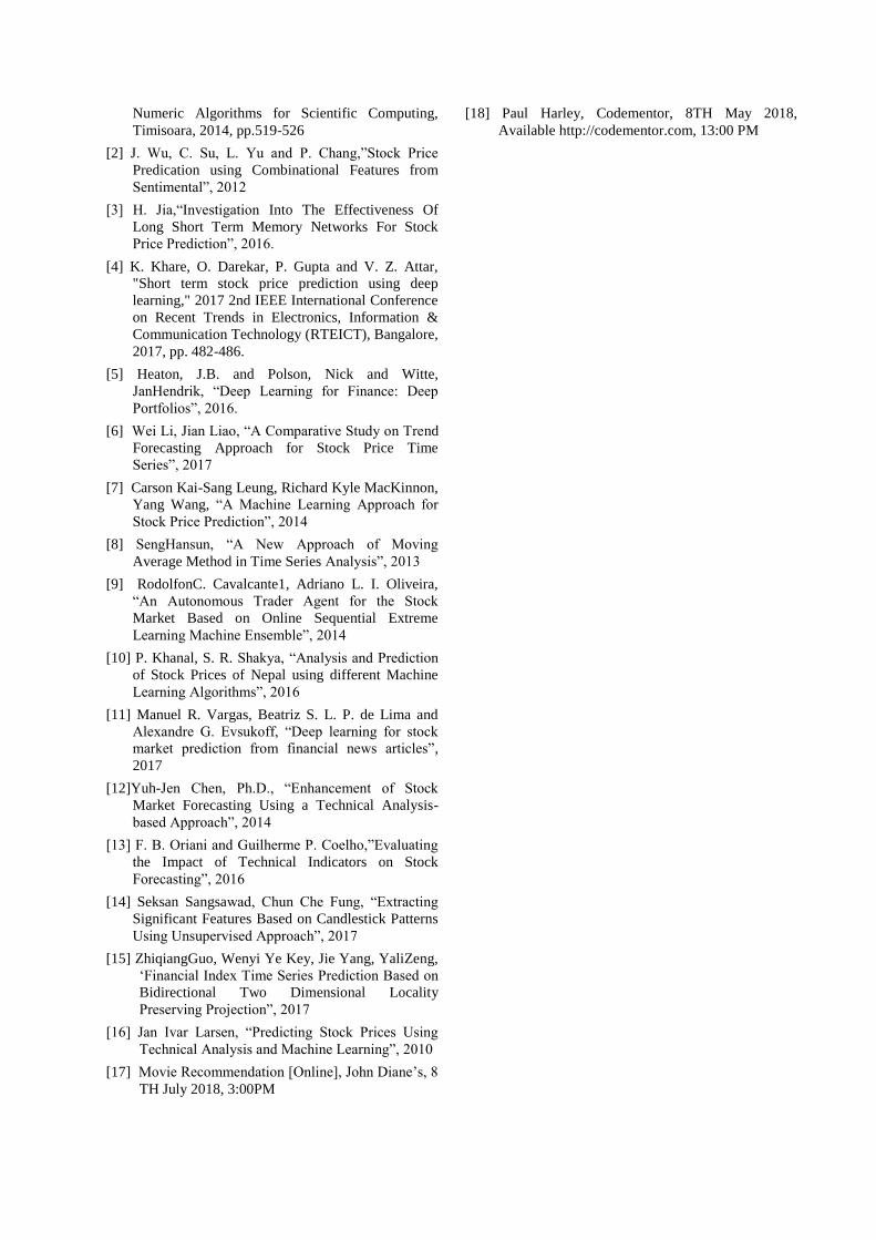
Figure 6: Actual vs. Forecasted: ADBL
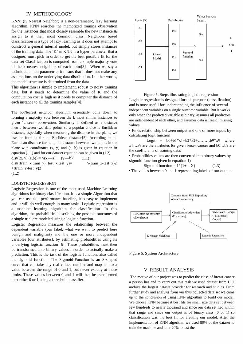
Figure 7: Actual vs. Forecasted: Nabil
The fig 6 and 7 shows the data of Agriculture
Development Bank Limited and Nabil Bank
respectively. A total of 3587 data were used for ADBL
and 4513 data were used for Nabil Bank for calculation
using only their Closing price and Date.
The result obtained in both the cases was fairly accurate
as from fig taken. The prediction is fairly accurate
unless there is huge and sudden variation in actual data.
On other hand, this also proves the hypothesis that stock
market is actually unpredictable. After the phase of
forecasting, the result will be displayed to the users in
the form of web pages which will benefit the financial
analysts, investors to take trading decision by observing
market behavior.
We obtained the MSE (Mean Square Error) using the
SARIMA model as 30.01 whereas the MSE using the
ARIMA model is 205.82. If Y' is a vector of n
predictions generated from a sample of n data points on
all variables, and Y is the vector of observed values of
the variable being predicted, then the within-sample
MSE of the predictor is computed as
MSE =
VIII.CONCLUSION
Financial analysts, investors can use this prediction
model to take trading decision by observing market
behavior. The system we have designed is quite simple
and works on time series analysis. While completing
the project various problems were tackled and resolved
to make the system more flexible. The project has been
a great learning experience for us. Importance of team
work is well understood through the project. This
project did provide us the opportunity to learn new
language Django, Python, also the practical approach of
software engineering. Thus, we can say that the project
was the great opportunity for us to test all the
knowledge we have gained over the years studying
engineering.
IX. REFERENCES [1] M. Tireaand V.Negru, “Intelligent Stock Market
Analysis System- A Fundamantal and
Macro-economical Analysis Approach”, 2014
16th International Symposium on Symbolic and
Numeric Algorithms for Scientific Computing,
Timisoara, 2014, pp.519-526
[2] J. Wu, C. Su, L. Yu and P. Chang,”Stock Price
Predication using Combinational Features from
Sentimental”, 2012
[3] H. Jia,“Investigation Into The Effectiveness Of
Long Short Term Memory Networks For Stock
Price Prediction”, 2016.
[4] K. Khare, O. Darekar, P. Gupta and V. Z. Attar,
"Short term stock price prediction using deep
learning," 2017 2nd IEEE International Conference
on Recent Trends in Electronics, Information &
Communication Technology (RTEICT), Bangalore,
2017, pp. 482-486.
[5] Heaton, J.B. and Polson, Nick and Witte,
JanHendrik, “Deep Learning for Finance: Deep
Portfolios”, 2016.
[6] Wei Li, Jian Liao, “A Comparative Study on Trend
Forecasting Approach for Stock Price Time
Series”, 2017
[7] Carson Kai-Sang Leung, Richard Kyle MacKinnon,
Yang Wang, “A Machine Learning Approach for
Stock Price Prediction”, 2014
[8] SengHansun, “A New Approach of Moving
Average Method in Time Series Analysis”, 2013
[9] RodolfonC. Cavalcante1, Adriano L. I. Oliveira,
“An Autonomous Trader Agent for the Stock
Market Based on Online Sequential Extreme
Learning Machine Ensemble”, 2014
[10] P. Khanal, S. R. Shakya, “Analysis and Prediction
of Stock Prices of Nepal using different Machine
Learning Algorithms”, 2016
[11] Manuel R. Vargas, Beatriz S. L. P. de Lima and
Alexandre G. Evsukoff, “Deep learning for stock
market prediction from financial news articles”,
2017
[12]Yuh-Jen Chen, Ph.D., “Enhancement of Stock
Market Forecasting Using a Technical Analysis-
based Approach”, 2014
[13] F. B. Oriani and Guilherme P. Coelho,”Evaluating
the Impact of Technical Indicators on Stock
Forecasting”, 2016
[14] Seksan Sangsawad, Chun Che Fung, “Extracting
Significant Features Based on Candlestick Patterns
Using Unsupervised Approach”, 2017
[15] ZhiqiangGuo, Wenyi Ye Key, Jie Yang, YaliZeng,
„Financial Index Time Series Prediction Based on
Bidirectional Two Dimensional Locality
Preserving Projection”, 2017
[16] Jan Ivar Larsen, “Predicting Stock Prices Using
Technical Analysis and Machine Learning”, 2010
[17] Movie Recommendation [Online], John Diane‟s, 8
TH July 2018, 3:00PM
[18] Paul Harley, Codementor, 8TH May 2018,
Available http://codementor.com, 13:00 PM

Breast Breast Cancer Prediction using Machine Learning Algorithm
Kritika Prasai Advanced College of Engineering and Management
Lalitpur, Nepal
Anjila Budhathoki Anku Jaiswal Lecturer Advanced College of Engineering and Management
Lalitpur, Nepal [email protected]
Abstract— The second important cause of cancer deaths in women
today is Breast Cancer and it is the most common type of cancer in
women. Disease diagnosis is one of the applications of AI which can be
implemented and are proving successful results. The main idea behind
this project is to see to what extent can machine learning algorithms be
used for detecting breast cancer of biopsied cells from women with
abnormal breast masses. To create the classifier, the WBCD
(Wisconsin Breast Cancer Diagnosis) dataset is employed [1]. This dataset is widely utilized for this kind of application
because it is virtually noise-free and has just a few missing values.
The objective of this project is we predict breast cancer tumors as
either Malignant (being cancerous) or Benign (being non-
cancerous) based on a given patient’s symptoms and attributes so
that we can pay proper attention towards health. The use of two
popular algorithm KNN (K Nearest Neighbors) and Logistic
regression is done in the project and hence based on their accuracy
which is very close to each other we used KNN for further
prediction. The performance of both algorithms is close to each
other. Accuracy of KNN is (97.84%) which is greater than logistic
(97.14%).Hence; we implemented KNN for prediction of breast
cancer.
Keywords— Wisconsin Breast Cancer Diagnosis,
Malignant, Benign, K nearest Neighbors, Logistic Regression
I. INTRODUCTION Looking back at the recent health statistics report it was found
that around 10 to 50% people get wrongly diagnosed of one or
other disease every year. And this condition is not so different
talking globally, so this is a problem for all. And here comes the
role of technology which can help solve these problems. This
will drastically reduce patient death, save medical practices a lot
of money, and aid doctors in the patient care process. It’s
important to remember that AI won't replace doctors; it will
become the most powerful tool they've ever used. And once
Advanced College of Engineering and
Management Lalitpur, Nepal
[email protected] enough AI startups start impacting the field of healthcare, it will become as common a tool as the stethoscope has been. As we all know cancer is one of the most feared diseases in the
world. Almost everyone knows someone who has been affected
by cancer. The rate of people getting cancer has increased
dramatically recently. External factors such as environment,
lifestyle, genetic, food intake and so on have played a
significant role in deciding whether a person would be suffering
from cancer or not. It was found that around 8.8 million deaths
occurred due to cancer in 2015 and is estimated to reach 12
million by 2030. In a country whose one third population is
women, we took an initiative in the topic of breast cancer. Breast cancer is the most prevalent cancer type in women in
most parts of the world. The disease is characterized by two
terms benign and malignant. The term "benign" refers to a
tumor, condition, or growth that is not cancerous. This means it
is localized and has not spread to other parts of the body or
invaded and destroyed nearby tissue. The opposite of benign is
“malignant” tumor. Malignant tumors are cancer, where the
cancer cells can invade and damage tissues and organs near the
tumor. Also, cancer cells can break away from a malignant
tumor and enter the lymphatic system or the bloodstream. Our project is based on implementation of machine learning
based algorithms to predict and diagnose the class of breast
cancer. In order to predict the class of breast cancer there has to
be a model with accurate prediction that will help the doctors to
diagnose the cancer whether it is benign or malignant. To
achieve the prediction model we implemented “KNN” as well
as “Logistic Regression” and tested the accuracy amongst these
two algorithms. It was found that KNN gave slightly more
accuracy than logistic so we implemented KNN to integrate our
project. This project is used to identify the breast cancer
condition whether it’s benign or malignant.

II. RELATED WORK New technologies like supervised learning, data analysis and
prediction, data mining and knowledge discovery have
developed allowing researchers and developers to discover
knowledge and find hidden patterns in large data sets[2] .
From our research we came up with few of the existing
technology that is used in disease prediction:
Brisk: For women with a family history of the disease, the app
walks them through their age-specific risk of developing the
disease, beginning with a question about whether the family
history involved a first-degree relative, a second-degree
relative, a mother and paternal aunt, and so on. The app
clearly cautions that it is not fail-safe. It is not a substitution
for a formal cancer risk assessment by a skilled physician. It
doesn’t include risk factors other than family history.
Breast Cancer Recurrence Score Estimator: Researchers from John Hopkins Kimmel Cancer Centre have
created a free of cost web-based app, designed to assist in the
prediction of the risk of the return of breast cancer in patients.
The app itself was created by Leslie Cope Ph.D., an associate
professor of oncology at the Johns Hopkins University School of
Medicine and Kimmel Cancer Centre member, with the help of a
team of graduate students who assisted with the coding. Called
the ‘Breast Cancer Recurrence Score Estimator’, it is possible to
use it for stage 1, 2, node negative and ER-positive breast
cancers. They developed the app based on data taken from over
1,113 patients’ medical records from five US hospitals. The
researchers then added additional information from 472 other
patients as a means of testing the estimator.
III. ABOUT THE DATASET For this project, The Wisconsin Breast Cancer dataset from the
University of California at Irvine (UCI) Machine Learning
Repository is used to differentiate benign (non-cancerous) from
malignant (cancerous) samples[1] . There are 699 number of
instances and 10 attributes plus the class attribute. In the given
data set, it had 16 missing attribute values. There are 16
instances that contain a single missing (i.e., unavailable)
attribute value, now denoted by "?". Data set characteristics is multivariate where attribute has
integer type characteristics. It has 2 class distribution having: Benign: 458 (65.5%) Malignant: 241 (34.5%)
Following Table 1 shows the description of breast cancer dataset
and Table 2 consists brief details of attributes present in dataset.
Table 1: Description of data set
Datasets Number of Number of Number of Number attributes instances classes of missing values Wisconsin 11 699 2 16 Breast
Cancer
(Original)
Table 2: Attribute of breast cancer dataset
Number Attribute Domain
1. Sample number ID Number
2. Clump Thickness 1-10
3. Uniformity of Cell Size 1-10
4. Uniformity of Cell Shape 1-10
5. Marginal Adhesion 1-10
6. Single Epithelial Cell Size 1-10
7. Bare Nuclei 1-10
8. Bland Chromatin 1-10
9. Normal Nucleoli 1-10
10. Mitoses 1-10
11. Class 1-10
Clump thickness: Benign cells tend to be grouped in monolayers,
while cancerous cells are often grouped in multilayer. Uniformity
of cell size/shape: Cancer cells tend to vary in size and shape.
That is why these parameters are valuable in determining
whether the cells are cancerous or not. Marginal adhesion: Normal cells tend to stick together. Cancer
cells tend to lose this ability. So loss of adhesion is a sign of
malignancy. Single epithelial cell size: Is related to the uniformity mentioned
above. Epithelial cells that are significantly enlarged may be a
malignant cell. Bare nuclei: This is a term used for nuclei that is not surrounded
by cytoplasm (the rest of the cell). Those are typically seen in
benign tumors. Bland Chromatin: Describes a uniform "texture" of the nucleus
seen in benign cells. In cancer cells the chromatin tends to be
coarser. Normal nucleoli: Nucleoli are small structures seen in the
nucleus. In normal cells the nucleolus is usually very small if
visible at all. In cancer cells the nucleoli become more
prominent, and sometimes there are more of them.
IV. METHODOLOGY KNN: (K Nearest Neighbor) is a non-parametric, lazy learning
algorithm. KNN searches the memorized training observation
for the instances that most closely resemble the new instance &
assign to it their most common class. Neighbors based
classification is a type of lazy learning as it does not attempt to
construct a general internal model, but simply stores instances
of the training data. The ‘K’ in KNN is a hyper parameter that a
designer, must pick in order to get the best possible fit for the
data set Classification is computed from a simple majority vote
of the k nearest neighbors of each point[3] . When we say a
technique is non-parametric, it means that it does not make any
assumptions on the underlying data distribution. In other words,
the model structure is determined from the data. This algorithm is simple to implement, robust to noisy training
data, but it needs to determine the value of K and the
computation cost is high as it needs to computer the distance of
each instance to all the training samples[4].
The K-Nearest neighbor algorithm essentially boils down to
forming a majority vote between the k most similar instances to
given ‘unseen’ observation. Similarity is defined as a distance
metric between two data points so a popular choice is Euclidean
distance, especially when measuring the distance in the plane, we
use the formula for the Euclidean distance[5]. According to the
Euclidean distance formula, the distance between two points in the
plane with coordinates (x, y) and (a, b) is given in equation in
equation (1.1) and for our dataset equation can be given in (1.2)
dist((x, y),(a,b)) = √(x — a)² + (y — b)² (1.1) dist((train_x,train_y),(test_x,test_y)= √(train_x-test_x)2 +(train_y-test_y)2 (1.2)
LOGISTIC REGRESSION Logistic Regression is one of the most used Machine Learning
algorithms for binary classification. It is a simple Algorithm that
you can use as a performance baseline, it is easy to implement
and it will do well enough in many tasks. Logistic regression is
a machine learning algorithm for classification. In this
algorithm, the probabilities describing the possible outcomes of
a single trial are modeled using a logistic function. Logistic Regression measures the relationship between the
dependent variable (our label, what we want to predict here
benign and malignant) and the one or more independent
variables (our attributes), by estimating probabilities using its
underlying logistic function [6]. These probabilities must then
be transformed into binary values in order to actually make a
prediction. This is the task of the logistic function, also called
the sigmoid function. The Sigmoid-Function is an S-shaped
curve that can take any real-valued number and map it into a
value between the range of 0 and 1, but never exactly at those
limits. These values between 0 and 1 will then be transformed
into either 0 or 1 using a threshold classifier.
Figure 5: Steps illustrating logistic regression Logistic regression is designed for this purpose (classification), and is most useful for understanding the influence of several independent variables on a single outcome variable. But it works only when the predicted variable is binary, assumes all predictors are independent of each other, and assumes data is free of missing values. • Finds relationship between output and one or more inputs by
calculating logit function Logit = b0+b1*x1+b2*x2+………b9*x9 where
x1…x9 are the attributes for given breast cancer and b0…b9 are
the coefficients of training data. • Probabilities values are then converted into binary values by
sigmoid function given in equation 1) Sigmoid function = 1/ (1+ e-X) (1.3)
• The values between 0 and 1 representing labels of our output.
Figure 6: System Architecture
V. RESULT ANALYSIS The motive of our project was to predict the class of breast cancer
a person has and to carry out this task we used dataset from UCI
archive the largest dataset provider for research and studies. From
further study and analysis from our thus collected data set we came
up to the conclusion of using KNN algorithm to build our model.
We choose KNN because it best fits for small size data set between
few hundreds to nearly thousand and since our data set lied within
that range and since our output is of binary class (0 or 1) so
classification was the best fit for creating our model. After the
implementation of KNN algorithm we used 80% of the dataset to
train the machine and later 20% to test the

accuracy of our model. Our data set consists of total of 699
instances among which Benign: 458 (65.5%) Malignant: 241
(34.5%). Using the train test split we could easily predict the
class of breast cancer as either benign or malignant and this
prediction model gave us a confidence level of 97.845%. Since
our goal was also to analyses the and accuracy of different
algorithms so we also tested our dataset using another algorithm
called Logistic Regression which gave us a confidence level of
(97.14%). From the final result after comparison we achieved
KNN slightly more precise in its prediction so we used KNN
based model to integrate it with our frontend and backend API. From the analysis above we can conclude that the model created gives excellent accuracy in predicting breast cancer from tumor data, therefore all the exploration and manipulation of the dataset were valid for this purpose. Hence from our project we were able
to build a tool for the doctors that will help them reduce the Figure 8: Prediction 1 inconsistency or misdiagnosis of disease. [7] For the further study between the datasets we performed correlation analysis and plotted a graph between attributes.
Figure 9: prediction 2
Figure 7: Correlation between attributes
Following is the table showing result of accuracy and algorithms: Table 3: Accuracy table
VI. CONCLUSION There are various data mining techniques available in medical
diagnosis, where the objective of these techniques is to assign a
patient to either a ‘healthy’ group that does not have a certain
disease or a ‘sick’ group that has strong evidence of having that
disease[8][9]. The system we have designed is quite simple and it
works both on Logistic Regression and KNN based algorithm.
From the analysis of the dataset we can conclude that the model we
have created gives us good accuracy in predicting breast cancer
from tumour data. Therefore all the exploration and manipulation
of the dataset were valid for this purpose and it highly increases the
accuracy of prediction. With the completion of this project we were
able to visualize the impact of data mining and machine learning
algorithms in the field of medicine [10]. Hence this project has
been a great learning experience for us.
VII. REFERENCES [1] Wolberg,H.W.(1992). UCI Repository of machine learning databases. Irvine, CA: University of California, Department of Information and Computer Science. [2] Wang, Haifeng & Yoon, Sang Won. (2015). Breast Cancer
Prediction Using Data Mining Method.

[3] Mucherino A., Papajorgji P.J., Pardalos P.M. (2009) k-
Nearest Neighbor Classification. In: Data Mining in
Agriculture. Springer Optimization and Its Applications, vol 34.
Springer, New York, NY [4] Li, S. (2017). Solving A Simple Classification Problem with
Python — Fruits Lovers’ Edition. [online] Towards Data
Science.2nd
July 2018,12:00PM
[5] Bronshtein.(2017)."A Quick Introduction to K-Nearest
Neighbors Algorithm".5th
July 2018,1:00 PM [6] Brownlee, J. (2016). Logistic Regression Tutorial for
Machine Learning. [online] Machine Learning Mastery.
Available at: https://machinelearningmastery.com/logistic-
regression-tutorial-for-machine-learnine. [7] Rodgers, J. L., & Nicewander, W. A. (1988). Thirteen
Ways to Look at the Correlation Coefficient. The American
Statistician, 42(1), 59-66. [8] Wang, Haifeng & Yoon, Sang Won. (2015). Breast Cancer
Prediction Using Data Mining Method. [9] Padmapriya, B & T, Velmurugan. (2014). A Survey on
Breast Cancer Analysis Using Data Mining Techniques.
10.1109/ICCIC.2014.7238530. [10] Shabani, Luzana & Raufi, Bujar & Ajdari, Jaumin &
Zenuni, Xhemal & Ismaili, Florie. (2017). Enhancing breast
cancer detection using data mining classification
techniques.Pressacademia.
Decentralized Application for Common Student Record onHyperledger Fabric
Kaushal Paudel Anku Jaiswal Arpan PokhrelDepartment of Electronics and Lecturer Department of Electronics and
Computer Engineering Department of Electronics and Computer Engineering
Advanced College of Engineering Computer Engineering Advanced College of Engineering and Management Advanced College of Engineering and Management
Lalitpur, Nepal and Management Lalitpur, [email protected] Lalitpur, Nepal [email protected]
Abstract—This paper describes the applicationwhich makes the record of students decentralizedwithin the network of Universities. Existing recordhandling method in educational sectors arecentralized. The very governing architecture leads tovulnerability in the loss of records on the failure ordamage of the central record storage facility. Inaddition, there is no transparency on the managementof records. In order to address these major issues, weimplemented distributed ledger technology alsoknown as blockchain technology. With the use ofblockchain technology a ledger is created anddistributed among the Universities, This makes theactivities more transparent and secured as everyactivity on the network is recorded on this ledger.Also, the records that one University stores record onthe local storage via an application, the record isdistributed among the participant of the network.Among numerous existing platform for
blockchain application development, weimplemented Hyperledger Fabric, HyperlegderComposer, and IBM Blockchain platform. Theresulting product is the composer application thatruns locally on the device and is connected to theIBM Blockchain services’ instance. This paperdescribes the development of a decentralizedapplication which is able to share the record amongthe participant of the network, on top of theHyperledger Fabric architecture.
Keywords—Blockchain, Hyperledger Fabric, Hyperledger Composer, IBM Blockchain Service
I. INTRODUCTION
The development of technology has formed a chainreaction on digitization. Currently, almost every pieceof data or information has been converted into digitalform. Nowadays even paper money is being replaced
by digital money. However, there are always newproblems arising with the development especially inthe technological field. The major problem which isdeveloping in the serious issue is the risk of losingdata. If the storage facility of any particular data isdamaged, the data is bound to disappear since digitalinformation is more vulnerable to even small risks. Ifdata is lost the retrieval is almost impossible. All ofthese major problems can be concluded to the singleproblem of centralized data architecture.
Prevention is better than cure. So making the record
secure can be the ultimate solution to guarantee its
security. One of the specific sector for decentralization of
data is records of educational sectors. Student’s records
are mainly the academic certificates that reflect the
qualification that they have achieved. These are the
valuable assets for the future use and are necessary for as
long as they live. Records of students can be viewed in
order to get the summary of the qualification and the
amount of knowledge they have. Eventually, for every
professional practice, these documents are compulsory.
Since records reflect the past, they need to be highlysecured. Otherwise, theoretically, the past is erased withthe damage on the records. The ease in accessibility andsecurity of these documents can provide huge comfort foranyone who is willing to protect their past. The written orhard copy of documents are very vulnerable to physicaldamage and in many cases, they get lost. The recovery ofthe document is inefficient as the data are centralized in asingle record system. The recovery of the documents takethe large amount of time, effort and it might cost somemoney as well. And if the single record system of theeducational sector gets damaged then the proof of recordis lost.
Decentralization of the records like academic
certificates not only makes the practices for student
easier but also make the whole system more meaningful
and efficient. Implementation of the decentralized
architecture of data makes the record secured, lessvulnerable to damage and eases the accessibility.
II. RELATED WORKS
Though there is an immense development of
distributed ledger technology in the area of
cryptocurrencies, the implementation in the business level
is not too popular. It has just started to catch the eye of
business companies for the implementation of record
handling. There are numerous other blockchain platforms
that offer the scripting. Ethereum and EOSIO are some of
those platforms. However, the Ethereum network is
public where every node is equal. This cannot help build
the business level applications. So, Hyperledger Fabric
and r3Corda are showing many implementations in small
organizations. In recent times distributed ledger
technology has been implemented in medical record
handling. MedRec is one of the blockchain applications
makes the medical records decentralized. In addition,
there are numerous ongoing distributed ledger
technologies fully contributed towards record
decentralization. Since this technology is coming forward
in recent times, only a few developed applications have
been produced and implemented in business level for
record decentralization.
BI. ABOUT HYPERLEDGER FABRIC
AND HYPERLEDGER COMPOSER
Hyperledger Fabric is one among manyHyperledger projects hosted by Linux Foundation.Hyperledger Fabric project has been supported andhugely promoted by IBM. The focal point of thisplatform is that it allows the permission network alongwith the implementation of unique architecture tofacilitate the business-level use cases. The primarygoal of this platform has been to enhance businesslevel use cases. The smart contract which is termed as‘Chaincode’ in the fabric network defines the type ofassets and transactions that run on the application.Chaincode that runs on the network is needed todevelop by programmers as desired for any particularfield.
Hyperledger Composer is one of the toolsets that
provides ease in the development of Hyperledger Fabric
Application. Using composer the application is modeled
in Composer Modelling Language and the logic of the
application can be written in programming languages
including, JavaScript, and Golang. Composer toolset
provides the developer a familiar environment for the
development of application since it
offers numerous familiar languages for coding and also offers a testing platform.
IV. HYPERLEDGER FABRIC
ARCHITECTURAL DESCRIPTION
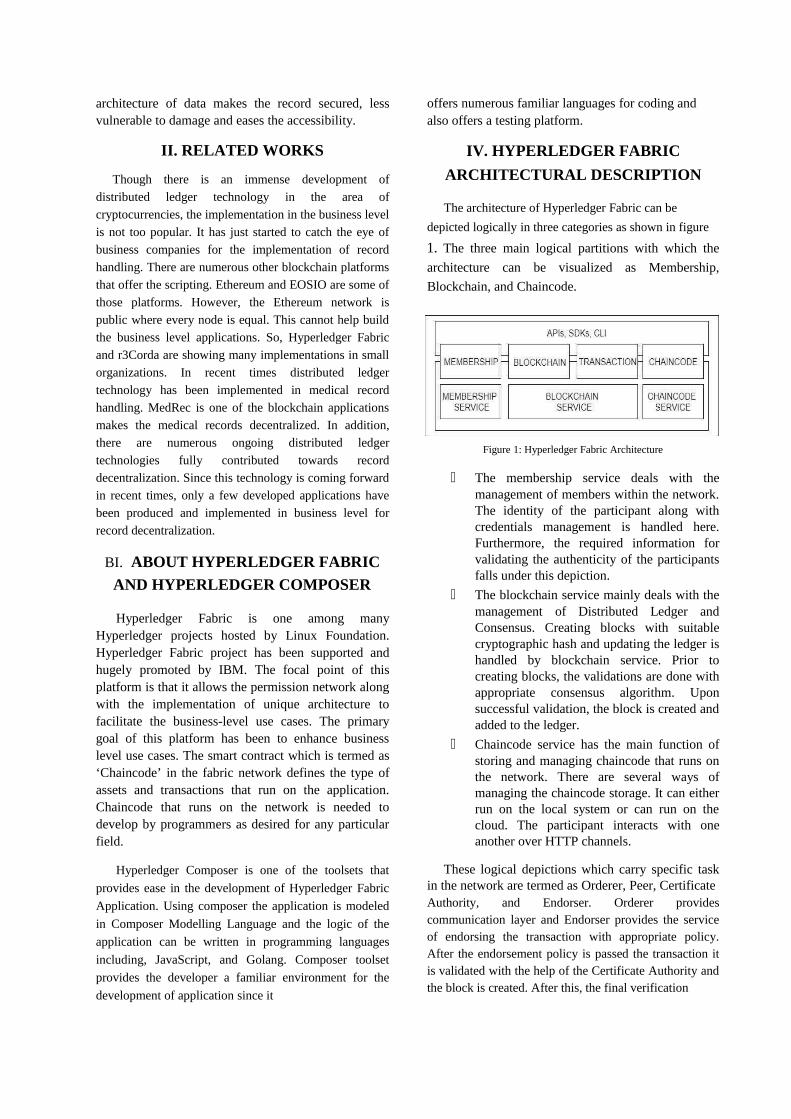
The architecture of Hyperledger Fabric can be
depicted logically in three categories as shown in figure
1. The three main logical partitions with which the
architecture can be visualized as Membership,
Blockchain, and Chaincode.
Figure 1: Hyperledger Fabric Architecture
The membership service deals with themanagement of members within the network.The identity of the participant along withcredentials management is handled here.Furthermore, the required information forvalidating the authenticity of the participantsfalls under this depiction.
The blockchain service mainly deals with themanagement of Distributed Ledger andConsensus. Creating blocks with suitablecryptographic hash and updating the ledger ishandled by blockchain service. Prior tocreating blocks, the validations are done withappropriate consensus algorithm. Uponsuccessful validation, the block is created andadded to the ledger.
Chaincode service has the main function ofstoring and managing chaincode that runs onthe network. There are several ways ofmanaging the chaincode storage. It can eitherrun on the local system or can run on thecloud. The participant interacts with oneanother over HTTP channels.
These logical depictions which carry specific taskin the network are termed as Orderer, Peer, CertificateAuthority, and Endorser. Orderer providescommunication layer and Endorser provides the serviceof endorsing the transaction with appropriate policy.After the endorsement policy is passed the transaction itis validated with the help of the Certificate Authority andthe block is created. After this, the final verification
is done by Peers and is decided to add to the ledger ornot.
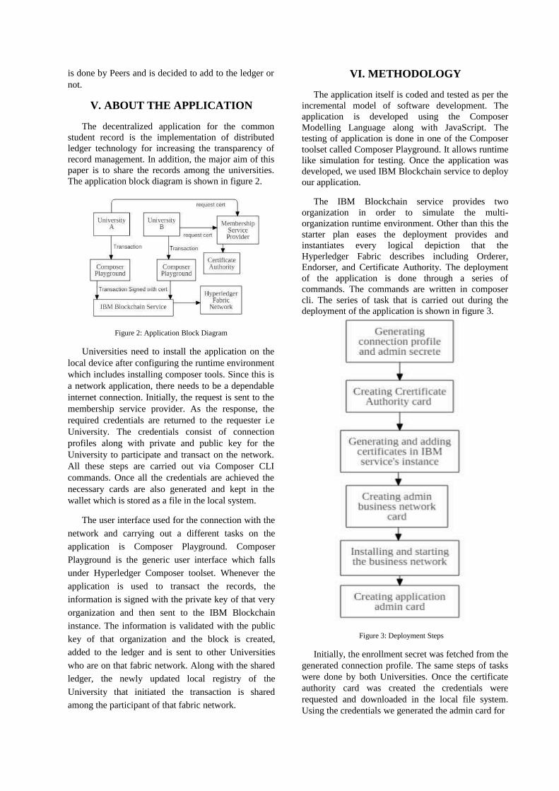
V. ABOUT THE APPLICATION
The decentralized application for the commonstudent record is the implementation of distributedledger technology for increasing the transparency ofrecord management. In addition, the major aim of thispaper is to share the records among the universities.The application block diagram is shown in figure 2.
Figure 2: Application Block Diagram
Universities need to install the application on thelocal device after configuring the runtime environmentwhich includes installing composer tools. Since this isa network application, there needs to be a dependableinternet connection. Initially, the request is sent to themembership service provider. As the response, therequired credentials are returned to the requester i.eUniversity. The credentials consist of connectionprofiles along with private and public key for theUniversity to participate and transact on the network.All these steps are carried out via Composer CLIcommands. Once all the credentials are achieved thenecessary cards are also generated and kept in thewallet which is stored as a file in the local system.
The user interface used for the connection with the
network and carrying out a different tasks on the
application is Composer Playground. Composer
Playground is the generic user interface which falls
under Hyperledger Composer toolset. Whenever the
application is used to transact the records, the
information is signed with the private key of that very
organization and then sent to the IBM Blockchain
instance. The information is validated with the public
key of that organization and the block is created,
added to the ledger and is sent to other Universities
who are on that fabric network. Along with the shared
ledger, the newly updated local registry of the
University that initiated the transaction is shared
among the participant of that fabric network.
VI. METHODOLOGY
The application itself is coded and tested as per theincremental model of software development. Theapplication is developed using the ComposerModelling Language along with JavaScript. Thetesting of application is done in one of the Composertoolset called Composer Playground. It allows runtimelike simulation for testing. Once the application wasdeveloped, we used IBM Blockchain service to deployour application.
The IBM Blockchain service provides twoorganization in order to simulate the multi-organization runtime environment. Other than this thestarter plan eases the deployment provides andinstantiates every logical depiction that theHyperledger Fabric describes including Orderer,Endorser, and Certificate Authority. The deploymentof the application is done through a series ofcommands. The commands are written in composercli. The series of task that is carried out during thedeployment of the application is shown in figure 3.
Figure 3: Deployment Steps
Initially, the enrollment secret was fetched from thegenerated connection profile. The same steps of taskswere done by both Universities. Once the certificateauthority card was created the credentials wererequested and downloaded in the local file system.Using the credentials we generated the admin card for

installing the application and later instantiating it. Whilestarting the business network both organizations’credentials were used in order to successfully start theapplication. Once this step was completed the composer-playground was locally-launched and the data of theapplication were locally stored.
VII. RESULTS
First, the distributed ledger technology wassuccessfully implemented to increase the transparencyof record management. Every time the transaction ismade as shown in figure 4, the action is recorded inthe ledger by the formation of a new block as shown infigure 6. Each block consists of its own unique id,what was the request and what change occurred on theregistry after a successful transaction as shown infigure 7.1 and figure 7.2.
Figure 4: Initiating transaction for new asset creation onUniversity A
Figure 5: Successful creation of new asset on University A assetregistry
Figure 6: Creation of new block
Figure 7.1: Block details (Timestamp and ID)
Figure 7.2: Block details (Output)
In addition, the identity of the organization thatperformed the transaction was also seen on the blockand the timestamp related to that transaction. Theregistry which is updated on one machine is sharedamong the participant i.e. another University on thenetwork as shown in figure 8. The same registry canbe seen by both Universities.
Figure 8: Shared registry on University B
VIII. CONCLUSION
We were able to implement the

distributedledger fortransparency of transactions on recordswith the help ofIBM Blockchain service and were able to share the data

among the participant of the network. We found thatthe decentralization of records is possible and canproduce some great benefits to overcome the issuesand problem faced with existing centralized system.
REFERENCES
[1] MedRec. [Online]. Available: https://medrec.media.mit.edu/technical/. [Accessed: 8-Jul-2018].
[2] “1.1 Introduction,” EOSIO Developer Portal -EOSIO Development Documentation. [Online].Available:https://developers.eos.io/eosio-home/docs. [Accessed: 11-Jul-2018].
[3] H. B. 10213791453123901, “Deploy a businessnetwork on (free) IBM Blockchain Starter Plan,”Hacker Noon, 17-Apr-2018. [Online].Available: https://hackernoon.com/deploy-a-business-network-on-free-ibm-blockchain-starter-plan-93fafb3dd997. [Accessed: 11-Jul-2018].
[4] Rajeev Sakhuja, “Blockchain Development onHyperledger Fabric using Composer,” Udemy.[Online]. Available:https://www.udemy.com/hyperledger/. [Accessed:1-Jun-2018].
[5] Matthew Golby-Kirk, David Gorman, andYogendra K. Srivastav, “Deploy a sampleapplication to the IBM Blockchain Platform StarterPlan,” The Analytics Maturity Model (IT Best Kept Secret Is Optimization), 14-Jul-2018. [Online]. Available: https://www.ibm.com/developerworks/cloud/libra ry/cl-deploy-fabcar-sample-application-ibm-blockchain-starter-plan/index.html. [Accessed: 30-Jul-2018].
[6] “Ethereum Homestead Documentation,” What isEthereum? - Ethereum Homestead 0.1documentation. [Online]. Available:http://www.ethdocs.org/en/latest/. [Accessed: 1-Jun-2018].
[7] “IBM Blockchain Platform,” IBM Watson.[Online]. Available: https://console.bluemix.net/docs/services/blockch ain/index.html#ibm-blockchain-platform.[Accessed: 5-Jul-2018].
[8] IBMBlockchain, “Blockchain Innovators: CreatingBNAfilesandDeployingChaincode(4/6),” YouTube, 12-Jun-2018. [Online]. Available: https://www.youtube.com/watch?v=iIjiA52fzPk& t=1027s. [Accessed: 11-Dec-2018].
[9] “Overview,” CMS.gov Centers for Medicare &Medicaid Services, 26-Mar-2012. [Online].Available:https://www.cms.gov/Medicare/E-Health/EHealthRecords/. [Accessed: 11-Jun-2018].
[10] “Welcome to Corda !,” The network - R3 CordaV3.0 documentation. [Online]. Available: https://docs.corda.net/#. [Accessed: 1-Dec-2018].
[11] “Welcome to Hyperledger Composer,”Hyperledger Composer - Create businessnetworks and blockchain applications quickly forHyperledger | Hyperledger Composer.[Online]. Available:https://hyperledger.github.io/composer/latest/introduction/introduction.html. [Accessed: 1-Jul-2018].
[12] “Zach Gollwitzer,” YouTube. [Online].Available:https://www.youtube.com/channel/UCDwIw3MiPJXu5SavbZ3_a2A/videos?disable_polymer=1.[Accessed: 11-Jul-2018].
[13] Morris, V., Adivi, R. and Asara, A. (2018).Developing a Blockchain Business Network withHyperledger Composer using theIBM Blockchain Platform Starter Plan. [ebook]IBM Corp. Available at:http://www.redbooks.ibm.com/redpapers/pdfs/redp5492.pdf [Accessed 1-Jul-2018].
[14] M. Gupta, BLOCKCHAIN FOR DUMMIES. S.l.: JOHN WILEY & SONS, 2018.

Nepali Sentiment Analysis using Neural Network
Dipesh DulalDepartment of Electronics and Computer EngineeringAdvanced College of Engineering and Management
Lalitpur, [email protected]
Dipesh ShresthaDepartment of Electronics and Computer EngineeringAdvanced College of Engineering and Management
Lalitpur, Nepal
Anku JaiswalLecturer
Department of Electronics and Computer EngineeringAdvanced College of Engineering and Management
Lalitpur, [email protected]
Gaurab SubediDepartment of Electronics and Computer EngineeringAdvanced College of Engineering and Management
Lalitpur, Nepal
Ram SapkotaDepartment of Electronics and Computer EngineeringAdvanced College of Engineering and Management
Lalitpur, Nepal
Abstract— Sentiment Analysis also known as opinionmining is the process of identifying and categorizingopinions are now being possible due to the abundanceof texts on the internet. For this, we have developed asystem to analyze sentiment in Nepali sentences usinga Recurrent Neural Network. The system is able toclassify the Nepali text sentences as either negative orpositive. We collected data from various newswebsites as well as from social media websites thenlabeled some data points and trained the neuralnetwork model to form the system that can classifysentiments. This paper deals with the collection ofdata, training the model to run inference on it. Theresults of this system show that the LSTM RNNapproach to sentiment analysis can obtain about 70%test accuracy on our self-created corpus.
Keywords— Natural Language Processing, MachineLearning, Neural Networks, Nepali Language,Sentiment Analysis
I. INTRODUCTIONAs motivated by the rapid growth of text data, textmining has been applied to discover hidden knowledgefrom a text in many applications and domains. Inbusiness sectors, great efforts have been made to find outcustomers’ sentiments and opinions, often expressed infree text, towards companies’ products and services.However, discovering sentiments and opinions throughmanual analysis of a large volume of textual data isextremely difficult. Hence, in recent years, there havebeen much interests in the natural language processingcommunity to develop novel text mining techniques withthe capability of accurately extracting customers’opinions from large volumes of unstructured text data.Among various opinion mining
tasks, there is sentiment classification which classifiespeople’s opinions as a positive or negative spectrum.
There has been an abundance of Nepali text data invarious Nepali news websites as well as social mediawebsites such as; onlinekhabar.com, ratopati.com,ekantipur.com, facebook.com etc. Comments and reviewsare being constantly made using Nepali Unicode whichprovides the ground from where the data can be collected.The Nepali language is morphologically rich andcomplex so the classifier needs to consider severalspecific language features before classifying text.Preprocessing data is one of the delicate stages in thesentiment analysis task [1].
The third section discusses the data used in this paper andtheir collection using web scraping techniques and withproper API’s. The fourth section deals with themethodology of data preprocessing and implementationof the system. The fifth section deals with results andshows how the accuracy of the model differs using thetraining data and testing data.
II. RELATED WORKThe bootstrap work done in the field of sentimentanalysis is by Peter D. Turney that classified thesentiment of reviews as recommended (thumbs up) andnot recommended (thumbs down) [2] receiving theaccuracy of 74%. Whereas in the case of NepaliSentiment Analysis there has not been a majorbreakthrough. Chandan Prasad Gupta and Bal KrishnaBal proposed [1] the system of detecting the sentiment inNepali texts using self-developed Nepali SentimentCorpus. They use lexical methods to classify the texts.

The major breakthrough in this field happened whenresearchers at Stanford University proposed therecurrent neural network system for noise reduction inautomatic speech recognition (ASR) system [3]. Thisgave a new approach to tackle sequential data in thefield of natural language processing and machinelearning in general. The recurrent neural network hasoutperformed different other models in this task ofanalyzing and processing sequential data such as asequence of text.
The paper [4] by Mikolov et. al. discusses the efficientestimation of word embedding using skip gramapproach which can be considered as one of thegroundbreaking works increasing the efficiency of theclassification system. Similarly, other various authorshave used various natural language processingtechniques to classify sentiment of texts in differentlanguages. Like in this paper [5] the author discussesthe approach taken to analyze Turkish political news.Also, in this paper [6] author have used a lexicon-based approach for classifying Indian text which islexically similar to the Nepali language.
III. ABOUT THE DATASETThe dataset used in this paper has been collected fromvarious news websites such as; bsgnews.com,annapurnapost.com, also from Facebook and Twitterfor realistic reviews and comments in Nepali languageand Nepali corpus dataset (16NepaliNews corpus)easily available from GitHub [7]. Web-Scrappingtechnologies like; Beautiful Soup for python has beenused to scrap the data from various news websitesmentioned above whereas API for the socialnetworking websites were also used. The followingtables show the sources of data along with theirnumbers.
Table 1: Data Sources with numbers
Source Number of Data16NepaliNews Corpus 14,364 ArticlesFacebook 5,021 CommentsTwitter 324 TweetsAnnapurnapost.com 400 ArticlesBsgnews.com 1000 Articles
IV. METHODOLOGYA. Data CollectionThe raw data from the websites were pre-processedbefore it could be used. Some of the processes forpreprocessing the data were:
● Removing all the HTML entities like; tags and images
● Removing all characters that are not Nepali Unicode
After preprocessing some of them were stored in aMySQL database for data labeling process and aremaining huge portion of data was stored in a file forcreating word embedding using word2vec algorithm[4]. Manual annotation of data was done using thelabeling system created by using web applicationcreated with PHP programming language; Laravelframework. The screenshot of the labeling applicationis shown below in figure 1.
Figure 1: Sentiment Labeling Screenshot
After the sentences were manually annotated using thelabeling system they were stored in JSON format in afile which is then later used for training the neuralnetwork.
B. Data PreprocessingAfter data is collected, it is processed and transformedinto the correct format so that the neural network canunderstand both inputs and outputs. The blockdiagram below shows the data preprocessing step ofthe project.
Figure 2: Block Diagram of Text Preprocessing
From the block diagram, the process is clear andfollowing sub-sections describes each step involved indata preprocessing process.

Tokenization
The raw data were broken down to sentences andthen to words. Sentences were separated bypunctuations such as (?,।,.) and words were separatedby commas and white spaces
Figure 3: Tokenization
Stop Words Removal
Stop words are highly frequent words in thecorpus that do not provide any value to analysis. Adictionary of stop words was created and the matchingwords were removed.
Figure 3: Stop Words Removal
Stemming
Snowball rule-based stemming algorithm [8] wasused for removing some of the stems of Nepalilanguage such as; ।।, ।।।, ।। etc.
Figure 3: Stemming
Word2Vec
The word tokens were converted into 300dimensioned feature vectors. These feature vectors orembedding vectors were created in such a way thatwords which are related with each other had vectorsnearest to each other. This is the application of thispaper [4], Efficient Estimation of WordRepresentations in Vector Space.
Thus, the unprocessed text sentences were convertedinto words embedding vector of Nx300 where Nrepresents the number of word tokens in the sentence.
For example: Nepali sentence “।।।। ।ि।।।।।।। ।।।P ।। P ।“ is converted to feature vectors as;[[ 0.22, 0.56, 0.70, 0.24, 0.11, …], [0.12, 0.22, 0.36,0.11, 0.33, …],..]
C. Neural Network ModelAfter text preprocessing the datasets were used tobuild the sentiment classifier. It is the final step inpreparing the model for classification. The labeleddata from the JSON file is then fed into the neuralnetwork as shown in figure 3 one by one after splittingthem into train and test samples.
Figure 3: RNN Block Diagram
The neural network consists of two LSTM (LongShort-Term Memory) Cells connected together in astack with the output of 128 dimensions to be reducedto 2-dimension vector using a dense layer. We usesoftmax cross-entropy as loss function to train theneural network optimized using Adam optimizer. Thefollowing line graph shows training accuracy duringthe training process.
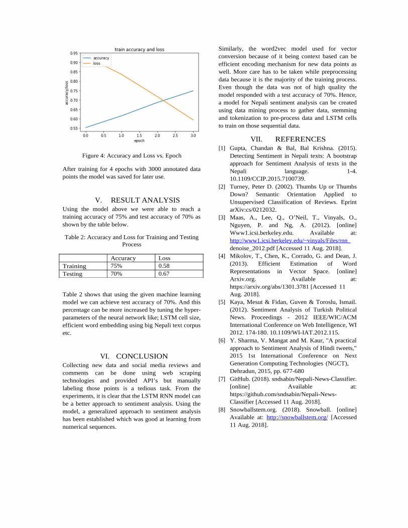
Figure 4: Accuracy and Loss vs. Epoch
After training for 4 epochs with 3000 annotated datapoints the model was saved for later use.
V. RESULT ANALYSISUsing the model above we were able to reach atraining accuracy of 75% and test accuracy of 70% asshown by the table below.
Table 2: Accuracy and Loss for Training and TestingProcess
Accuracy LossTraining 75% 0.58Testing 70% 0.67
Table 2 shows that using the given machine learningmodel we can achieve test accuracy of 70%. And thispercentage can be more increased by tuning the hyper-parameters of the neural network like; LSTM cell size,efficient word embedding using big Nepali text corpusetc.
VI. CONCLUSIONCollecting new data and social media reviews andcomments can be done using web scrapingtechnologies and provided API’s but manuallylabeling those points is a tedious task. From theexperiments, it is clear that the LSTM RNN model canbe a better approach to sentiment analysis. Using themodel, a generalized approach to sentiment analysishas been established which was good at learning fromnumerical sequences.
Similarly, the word2vec model used for vectorconversion because of it being context based can beefficient encoding mechanism for new data points aswell. More care has to be taken while preprocessingdata because it is the majority of the training process.Even though the data was not of high quality themodel responded with a test accuracy of 70%. Hence,a model for Nepali sentiment analysis can be createdusing data mining process to gather data, stemmingand tokenization to pre-process data and LSTM cellsto train on those sequential data.
VII. REFERENCES[1] Gupta, Chandan & Bal, Bal Krishna. (2015).
Detecting Sentiment in Nepali texts: A bootstrapapproach for Sentiment Analysis of texts in theNepali language. 1-4.10.1109/CCIP.2015.7100739.
[2] Turney, Peter D. (2002). Thumbs Up or ThumbsDown? Semantic Orientation Applied toUnsupervised Classification of Reviews. EprintarXiv:cs/0212032.
[3] Maas, A., Lee, Q., O’Neil, T., Vinyals, O.,Nguyen, P. and Ng, A. (2012). [online]Www1.icsi.berkeley.edu. Available at:http://www1.icsi.berkeley.edu/~vinyals/Files/rnn_denoise_2012.pdf [Accessed 11 Aug. 2018].
[4] Mikolov, T., Chen, K., Corrado, G. and Dean, J.(2013). Efficient Estimation of WordRepresentations in Vector Space. [online]Arxiv.org. Available at:https://arxiv.org/abs/1301.3781 [Accessed 11Aug. 2018].
[5] Kaya, Mesut & Fidan, Guven & Toroslu, Ismail.(2012). Sentiment Analysis of Turkish PoliticalNews. Proceedings - 2012 IEEE/WIC/ACMInternational Conference on Web Intelligence, WI2012. 174-180. 10.1109/WI-IAT.2012.115.
[6] Y. Sharma, V. Mangat and M. Kaur, "A practicalapproach to Sentiment Analysis of Hindi tweets,"2015 1st International Conference on NextGeneration Computing Technologies (NGCT),Dehradun, 2015, pp. 677-680
[7] GitHub. (2018). sndsabin/Nepali-News-Classifier.[online] Available at:https://github.com/sndsabin/Nepali-News- Classifier [Accessed 11 Aug. 2018].
[8] Snowballstem.org. (2018). Snowball. [online]Available at: http://snowballstem.org/ [Accessed11 Aug. 2018].

Cryptocurrency Trend Analysis and Correlation with
Twitter Sentiment
Prasanga Neupane, Anuj Poudel, Anup Kumar Pokhrel, Bishnu Kumar Lama, Dibakar Raj Pant
Department of Electronics and Computer Engineering, Central Campus Pulchowk
I.O.E, Tribhuvan University
Lalitpur, Nepal
Abstract - This research is concerned with predicting the
fluctuations in the volatile price of Bitcoin, which is nowadays
increasingly used for online transactions worldwide and are
considered as the global standard for transactions in the near
future. Bitcoin lacks central governing authority and is built on a
decentralized, peer-to-peer network with transactions being
carried out by the members of the network which may be any
general public. Thus daily transaction, trader’s activities and
general opinion of people towards Bitcoin can have direct or
indirect influence on its market value. Twitter being one of the
influential social media with many authentic news accounts is
selected as a source of news related to Bitcoin for this research. A
sentiment analysis system is devised using Linear Support Vector
Classifier which gives either positive or negative label to each tweet
from the news corpus with the accuracy of 84.43%. Then the
sentiment score of each day is analyzed for cross correlation with
corresponding price of Bitcoin of the same day which implied
sentiment of today has maximum impact on price of tomorrow.
Therefore to predict the increase or decrease of the price for the
following day a Naïve Bayes classifier is trained with sentiment
score and price which yielded an accuracy of 78.03%.
Index Terms – Bitcoin, Sentiment, Linear Support Vector, News
Corpus, Cross-Correlation, Naïve Bayes.
I. INTRODUCTION
Cryptocurrency [1] is digital currency governed by
cryptographic protocol which uses Blockchain [1]. The
continuous increase in adoption and widespread usage has
increased its value in real world applications by substantial
amount. Various cryptocurrencies have been invented since
2009 but the first one to be launched as a cryptocurrency was
Bitcoin [2]. It is a form of electronic cash with no governing
financial institution which can be used for online transactions
or as exchange between any two parties. Nowadays due to its
fluctuating and big-ticket value lion’s share of bitcoin
transactions occurs in exchange as a stock market rather than in
online merchant transactions.
However, it does not have central governing authority and is
controlled by the general public. We have seen a sea-change in
its price from nothing to 17,900 USD (January, 2018) within
the period of eight years. By this reason, Bitcoin is considered
a very volatile currency and its price is seen to have been
affected by socially constructed opinions over the internet.
II. LITERATURE REVIEW
In the work of Kristoufek [3] it is shown that some of the
extreme drops as well as price increases in the Bitcoin exchange
rate coincided with dramatic events in China. In another
research carried out by American Institute for Economic
Research (AIER) [4] shows a major fluctuation in price of
bitcoin driven by the impactful news and sentiment over the
world during the time period between 2016 and 2017.
The work of J. Bean [5] provides Twitter opinion mining idea
in order to visualize the general customer attitude and
satisfaction towards the airline company. Further, Nagar and
Hahsler [6] suggests a strong correlation exists between the
sentiment of news extracted the news corpus and the stock price
movement.
Colianni et. al. [7], have used Naive Bayes to find optimal time
to trade by correlating prices with Twitter. Pagolu et. al. [8]
work on predicting stock through twitter sentiment presents
strong correlation between Twitter sentiment and stock price
movement.
First of all, it is better to have a domain specific sentiment
analyser rather than general sentiment classification tool. For
that reason, a sentiment analyser specific to Cryptocurrency
news and statements is developed.
Furthermore, a correlation analysis is performed between the
historical price of Bitcoin and its corresponding sentiment score
to identify the extent of correlation. Then a new technique of
using sentiment score to visualize the fluctuating trend on the
Bitcoin’s price is used. The sentiment score - total percentage
of positive and negative sentiment score - of the day is used as
indicator for the price fluctuations.
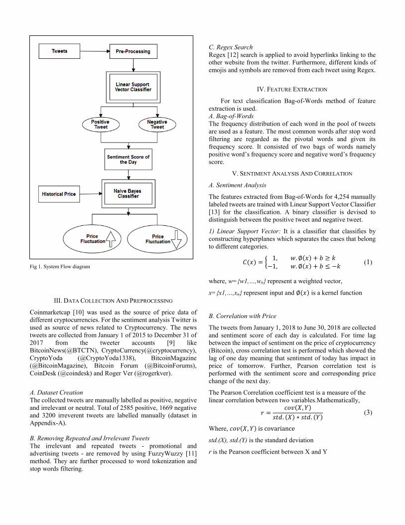
Fig 1. System Flow diagram
III. DATA COLLECTION AND PREPROCESSING
Coinmarketcap [10] was used as the source of price data of
different cryptocurrencies. For the sentiment analysis Twitter is
used as source of news related to Cryptocurrency. The news
tweets are collected from January 1 of 2015 to December 31 of
2017 from the tweeter accounts [9] like
BitcoinNews(@BTCTN), CryptoCurrency(@cryptocurrency),
CryptoYoda (@CryptoYoda1338), BitcoinMagazine
(@BitcoinMagazine), Bitcoin Forum (@BitcoinForums),
CoinDesk (@coindesk) and Roger Ver (@rogerkver).
A. Dataset Creation
The collected tweets are manually labelled as positive, negative
and irrelevant or neutral. Total of 2585 positive, 1669 negative
and 3200 irreverent tweets are labelled manually (dataset in
Appendix-A).
B. Removing Repeated and Irrelevant Tweets
The irrelevant and repeated tweets - promotional and
advertising tweets - are removed by using FuzzyWuzzy [11]
method. They are further processed to word tokenization and
stop words filtering.
C. Regex Search
Regex [12] search is applied to avoid hyperlinks linking to the
other website from the twitter. Furthermore, different kinds of
emojis and symbols are removed from each tweet using Regex.
IV. FEATURE EXTRACTION
For text classification Bag-of-Words method of feature
extraction is used.
A. Bag-of-Words
The frequency distribution of each word in the pool of tweets
are used as a feature. The most common words after stop word
filtering are regarded as the pivotal words and given its
frequency score. It consisted of two bags of words namely
positive word’s frequency score and negative word’s frequency
score.
V. SENTIMENT ANALYSIS AND CORRELATION
A. Sentiment Analysis
The features extracted from Bag-of-Words for 4,254 manually
labeled tweets are trained with Linear Support Vector Classifier
[13] for the classification. A binary classifier is devised to
distinguish between the positive tweet and negative tweet.
1) Linear Support Vector: It is a classifier that classifies by
constructing hyperplanes which separates the cases that belong
to different categories.
𝐶(𝑥) = {
1, 𝑤. ∅(𝑥) + 𝑏 ≥ 𝑘
−1, 𝑤. ∅(𝑥) + 𝑏 ≤ −𝑘 (1)
where, w={w1,…,wn} represent a weighted vector,
x={x1,…,xn} represent input and ∅(𝑥) is a kernel function
B. Correlation with Price
The tweets from January 1, 2018 to June 30, 2018 are collected
and sentiment score of each day is calculated. For time lag
between the impact of sentiment on the price of cryptocurrency
(Bitcoin), cross correlation test is performed which showed the
lag of one day meaning that sentiment of today has impact in
price of tomorrow. Further, Pearson correlation test is
performed with the sentiment score and corresponding price
change of the next day.
The Pearson Correlation coefficient test is a measure of the
linear correlation between two variables.Mathematically,
𝑟 =
𝑐𝑜𝑣(𝑋, 𝑌)
𝑠𝑡𝑑. (𝑋) ∗ 𝑠𝑡𝑑. (𝑌) (3)
Where, 𝑐𝑜𝑣(𝑋, 𝑌) is covariance
std.(X), std.(Y) is the standard deviation
r is the Pearson coefficient between X and Y

V. NAÏVE BAYES CLASSIFIER
The Naïve Bayes Classifier is trained with three features:
sentiment score of the day, corresponding market price of
Bitcoin and rise or fall (rise as 1 and fall as 0) of price next day.
A) Naïve Bayes
It is a conditional probability model which assumes that
features are statistically independent of one another.
Mathematically,
𝑝(𝐶𝑘|𝑥) =
𝑝(𝐶𝑘)𝑝(𝑥|𝐶𝑘)
𝑝(𝑥) (2)
Where,
𝑝(𝐶𝑘) is prior probability of class 𝐶𝑘
𝑝(𝑥|𝐶𝑘) is class conditional feature probability
𝑝(𝐶𝑘|𝑥) is probability x belonging to class 𝐶𝑘
VI. RESULTS AND ANALYSIS
All of the following study were carried out with the price data
and sentiment data related to Bitcoin from January 1st 2018 to
June 30th 2018.
The overall accuracy of sentiment classification by Linear
Support Vector Classifier with validation split of 1:3 is
achieved as 84.43% as shown in table below:
Table I. Confusion Matrix
Accuracy Precision Sensitivity Specificity
84.43% 87.89% 80.17% 88.76%
Confusion Matrix for LSVC for Sentiment Classification
The confusion matrix exhibits greater specificity than
sensitivity which implies that the model is better at classifying
the negative sentiments than it is for positive sentiments.
The Pearson Correlation Coefficient calculated between the
sentiment score and percentage price change of the next day
between the periods of January 1, 2018 to June 30, 2018 is given
in the table below:
Table II. Sentiment and Price Correlation
Price Fluctuation Pearson Correlation
Coefficient
More than
4%( approx.500 USD)
Negative Sentiment:0.41
Positive Sentiment: 0.26
Pearson Correlation Coefficient Comparison for different range of price
As Table-III shows, for the price fluctuations more than 4% (ie.
more than $500 during that study period) in a single day,
Pearson correlation coefficient is found to be 0.41 for negative
sentiment and corresponding fall in price and 0.26 between the
positive sentiment and its corresponding increase in price. This
shows there is a moderate (according to Evans 1996) [14]
correlation between rise of negative sentiment and consequent
fall in price of Bitcoin but a weak relation between increase of
positive sentiment and consequent increase in price.
The prediction accuracy for Naïve Bayes model for predicting
the direction of movement of price for the next day is found to
be 78.03% (when provided with price and sentiment score of
the day).
Table III. Confusion Matrix
Accuracy Precision Sensitivity Specificity
78.03% 85.27% 71.18% 85.89%
Confusion Matrix for Naïve Bayes Classifier for predicting direction of price
movement
The confusion matrix shows greater Specificity than sensitivity
which means that the model predicts more precisely to the fall
of price rather than for the increase in price.
VII. CONCLUSION
The major contribution of this work is a sentiment analyser
system which can distinguish between the positive and negative
tweets of Bitcoin over the Twitter with the accuracy of 84.43%.
Furthermore, the Naïve Bayes model which can predict the
direction of price movement for the next day is another useful
accomplishment. It also shows a moderate correlation of 0.41
between rise of negative opinions in the Twitter related to
Bitcoin and its consequent fall in price.
ACKNOWLEDGMENT
The authors would like to acknowledge Mr. Sandip Pandey
for his laudable contribution during this research work.
REFERENCES
[1] U. W. Chohan, “Cryptocurrencies: A Brief Thematic Review”, SSRN Electronic Journal, 2017.
[2] S. Nakamoto, Bitcoin: A peer-to-peer electronic cash system., 2008. [3] L. Kristoufek, "What are the main Drivers of the Bitcoin Price? Evidence
from Wavelet Cohernce Analysis", 2015. [4] “Bitcoin largest price changes coincide major News events about
Cryptocurrency” [Online]. Available: www.aier.org [Accessed 13 July 2018]
[5] J. Bean, "R by example: Mining Twitter for consumer attitudes towards airlines", 2011.
[6] A. Nagar and M. Hashler, "Using text and data mining techniques to
extract stock," vol. XX, 2012. [7] S.Colianni, S. Rosales and M. Signorotti, “Algorithmic trading of
cryptocurrency based on Twitter sentiment analysis.” , 2015 [8] V. Sasank Pagolu, K.N. Reddy,G. Panda and B. Majhi "Sentiment analysis
of Twitter data for predicting stock market movements",SCOPES, 2016. [9] Tweeter Accounts:
‘BitcoinNews’ Available: https://twitter.com/BTCTN?lang=en

‘CryptoCurrency’ Available: https://twitter.com/cryptocurrency?lang=en
‘CryptoYoda’ Available: https://twitter.com/CryptoYoda1338?lang=en
‘BitcoinMagzine’Available: https://twitter.com/bitcoinmagazin?lang=en
‘BitcoinForum’Available:https://twitter.com/BitcoinForumCom?lang=en
‘CoinDesk’ Available: https://twitter.com/coindesk?lang=en ‘RogerVer’ Available: https://twitter.com/rogerkver?lang=en
[10] Coin Market Cap, Available: https://coinmarketcap.com/
[Accessed 22 July 2018] [11] FuzzyWuzzy, "Geeksforgeeks.org," [Online]. Available:
https://www.geeksforgeeks.org/fuzzywuzzy-python-library/.[Accessed
24 July 2018].
[12] C. Frenz, “Introduction to Searching with Regular Expressions”,
Proceedings of the 2008 Trenton Computer Festival, 2008
[13] C. Cortes and V. Vapnik, "Support-vector networks". Machine
Learning,1995
[14] J. D. Evans, Straightforward statistics for the behavioral sciences, Brooks/Cole Publishing, 1996
APPENDIX-A
Some example of positive and negative labelled Tweets during creation of Dataset
Positive Tweets Negative Tweets
1. Church in Z rich Accepts Donations in Bitcoin, BCH,
Ether, Ripple and Stellar
2. Overall Capital of Crypto Markets Exceeds $750
Billion.
3. Turkish Minister Proposes National Cryptocurrency.
4. Amazon set to use Bitcoin as payment for
people.#Bitcoin
5. Australian Gold Refinery Announces Plan to Develop
Cryptocurrency #Bitcoin
1. Trader in Chicago Firm Stole Million BTC and Faces 20
Year Sentence #Bitcoin
2. Cryptocurrency Regulator Found Dead at His Home in
South Korea #Bitcoin
3. Lawyers Discuss Challenges Posed by Cryptocurrencies
During Divorce #Bitcoin
4. Scammers Are Ruining Crypto Twitter and Twitter Is to
Blame #Bitcoin
5. US Navy Bust Bitcoin Drug in Naval Academy #Bitcoin
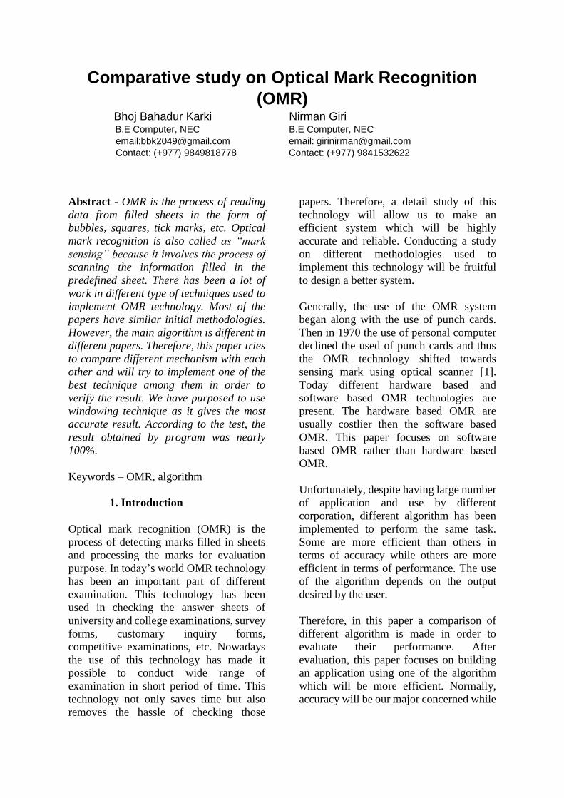
Comparative study on Optical Mark Recognition
(OMR) Bhoj Bahadur Karki Nirman Giri B.E Computer, NEC B.E Computer, NEC
email:[email protected] email: [email protected]
Contact: (+977) 9849818778 Contact: (+977) 9841532622
Abstract - OMR is the process of reading
data from filled sheets in the form of
bubbles, squares, tick marks, etc. Optical
mark recognition is also called as “mark
sensing” because it involves the process of
scanning the information filled in the
predefined sheet. There has been a lot of
work in different type of techniques used to
implement OMR technology. Most of the
papers have similar initial methodologies.
However, the main algorithm is different in
different papers. Therefore, this paper tries
to compare different mechanism with each
other and will try to implement one of the
best technique among them in order to
verify the result. We have purposed to use
windowing technique as it gives the most
accurate result. According to the test, the
result obtained by program was nearly
100%.
Keywords – OMR, algorithm
1. Introduction
Optical mark recognition (OMR) is the
process of detecting marks filled in sheets
and processing the marks for evaluation
purpose. In today’s world OMR technology
has been an important part of different
examination. This technology has been
used in checking the answer sheets of
university and college examinations, survey
forms, customary inquiry forms,
competitive examinations, etc. Nowadays
the use of this technology has made it
possible to conduct wide range of
examination in short period of time. This
technology not only saves time but also
removes the hassle of checking those
papers. Therefore, a detail study of this
technology will allow us to make an
efficient system which will be highly
accurate and reliable. Conducting a study
on different methodologies used to
implement this technology will be fruitful
to design a better system.
Generally, the use of the OMR system
began along with the use of punch cards.
Then in 1970 the use of personal computer
declined the used of punch cards and thus
the OMR technology shifted towards
sensing mark using optical scanner [1].
Today different hardware based and
software based OMR technologies are
present. The hardware based OMR are
usually costlier then the software based
OMR. This paper focuses on software
based OMR rather than hardware based
OMR.
Unfortunately, despite having large number
of application and use by different
corporation, different algorithm has been
implemented to perform the same task.
Some are more efficient than others in
terms of accuracy while others are more
efficient in terms of performance. The use
of the algorithm depends on the output
desired by the user.
Therefore, in this paper a comparison of
different algorithm is made in order to
evaluate their performance. After
evaluation, this paper focuses on building
an application using one of the algorithm
which will be more efficient. Normally,
accuracy will be our major concerned while

choosing algorithm rather than
performance.
2. Literature review
2.1. A low-cost OMR Solution for
Educational Application, Hui Deng, Feng
Wang, Bo Liang [2]:
This paper is based on reducing the cost that
arises when checking OMR sheets using
different hardware and software. Often
different hardware and software uses high
quality papers (90-110 GSM) but the
normal papers are between 60-70GSM. The
availability of such high quality paper is
costlier. Therefore, this method was
introduced. They have following steps for
the system design:
a. A Microsoft Word macro-based sheet
design technique to simplify the design
of questionnaire.
b. Low cost image-based OMR technique
and the images can be obtained from any
kinds of scanner.
3. Global and regional area image
deformation corrections to improve the
recognition precision.
The sheet sample contains marking area as
other normal sheet but they had “L” shaped
dark circular plot which they used to get the
exact position for different mark answers
using flag point searching algorithm. In flag
point searching, they performed horizontal
and vertical search. They performed
vertical searching from top left portion and
then they performed horizontal searching
form bottom left section.
Main Algorithm:
The main algorithm used for searching
mark was flag point searching where they
searched in two ways one horizontal and
one vertical for the mark based on the
coordinate system of the “L” shaped flag.
Accuracy and Result:
They performed different test and found out
that they could get 98% accuracy by using
this technique. The 100% accuracy could
not be obtained because of the two main
reasons, one ink infiltration and second due
to the distortion of the thin paper.
2.2. Robust and Low-Cost Optical Mark
Recognition for Automated Data Entry,
Parinya Sanguansat [3]:
This paper presents an automated data entry
method. This provides user with different
answer filling method such as bubble, tick-
mark and cross-mark. The result for
bubbles was better than other options. The
design of the sheet contains three corner for
detecting the alignment of the sheets.
Main Algorithm:
The backward difference method was used
for detection of coroner points and other
bubbles. This method is represented by
following equation:
∆𝑅[𝑖] = 𝑅[𝑖] − 𝑅[𝑖 − 1] =
{
−1 , 𝑅[𝑖] < 𝑅[𝑖 − 1]
0 , 𝑅[𝑖] = 𝑅[𝑖 − 1]
1 , 𝑅[𝑖] > 𝑅[𝑖 − 1]
---(1)
Where the 𝑅[𝑖] is the 𝑖 − 𝑡ℎ pixel position
in the row or column. ∆𝑅[𝑖] is calculated by
differencing the shifted version of the 𝑅[𝑖] itself. The value of the difference is used for
pixel transition. This equation was used for
corners detection which was used for
alignment of the paper and, also used for
inner bubble detection which was further
processed for template matching.
Accuracy and Result:
After applying this technique, it was found
that the accuracy for the bubbles, tick mark,

cross mark, were 100%, 85.72%,94.29%,
respectively.
2.3. A generalized approach to Optical
Mark Recognition, Surbhi Gupta, Geetila
Singla, and Parvinder Singh Sandhu [4]:
This paper presents an overall technique
while making an OMR software. First the
image was scanned and various image
processing algorithm were implemented for
effective scanning of OMR sheet.
Techniques presented:
I. 2-D transformation: The shape, size,
orientation of the sheet plays vital role in
the scanning of the OMR sheet. Following
transformation were used:
a. Translation: It is the process of
repositioning a point along a straight line. If
( 𝑥2, 𝑦2) is translation of factor ‘t’ in original
coordinate (x, y), then ( 𝑥2, 𝑦2) can be
presented as
𝑥2= x + t x;
𝑦2 = y + t y;
b. Rotation: In this technique the sheet is
rotated by certain angle along the centre
coordinate of the system. The rotating angle
is calculated by taking arc tan of y and x
coordinate of its corresponding corner
points.
c. Scaling: It is the technique of resizing of
the sheet by certain value. This is done in
order to make the scan coordinate lie in
desired position while processing for mark.
II. Circle generating algorithm: This
algorithm is based on filling the mark
properly if some portion of the mark has not
been filled. This allows for higher reading
accuracy and proper calculation of central
position of the detected mark. We need to
determine the centre position of a mark in
order to compare it with a template value.
III. Area fill algorithm: This algorithm
serves same thing as circle generating
algorithm. Author presented it in order to
show any method can be used for filling a
region. Here the filling starts from inside
and moves outside. The filling can also start
form outside toward inside but generally
inside-out filling is preferred.
Accuracy and Result:
This paper presented a general approach
required while making an OMR system. So
the accuracy and result might vary based on
different other technique used along with
these techniques by OMR system designer.
2.4 Cost Effective Optical Mark Reader,
Rakesh S, Kailash Atal, Ashish Arora [5]:
This paper presented a cost effective way of
implementing OMR software. It focused on
image processing techniques and software
based OMR system. A sheet was scanned
and processed through different image
processing methods. For identifying filled
bubbles, it used grayscale method. It
implemented parallel processing in order to
increase the performance of scanning form.
It had processing rate of 400 sheets per
minutes.
Main algorithms:
It used the same techniques as used by
above methods for alignment and proper
adjustment of sheets such as scanning for
corner points and translation, rotation,
scaling and region detection.
The main difference was in finding out the
filled in bubbles. It used to find threshold
value and implemented the greyscale
technique. According to this technique, the
minimum (Vmin) and maximum (Vmax),
average greyscale value of all the bubbles is
computed. The bubble (Vi) is said to be

filled if it is closer to Vmin and lower than
Vmax, i.e.
Vi< Vmin+ (Vmax– Vmin) * p
And the bubble is said to be unfilled if Vi
is,
Vi> Vmin+ (Vmax– Vmin) * q
Here the p and q are the adaptive threshold
value. They had taken p=0.4 and q = 0.6,
these value might differ based on the sheet
taken in consideration and filled in bubbles.
After the filled bubbles was detected it was
compared with the correct answer sheet
template.
Accuracy and Result:
The accuracy rate using this technique was
99.20%.
2.5. AUTOMATIC OMR ANSWER
SHEET CHECKER, MS. VRUSHABHA
MURAMKAR, PROF. SACHIN
AGARWAL [6]:
This paper presented cost effective OMR
software using template matching
technique. The image is converted into
binary image, before processing it to find
the accurate coordinates and finally the
overall answer.
Main algorithm:
The main algorithm used in this paper was
point correlation algorithm. In this
algorithm instead of matching entire answer
sheet to the actual template, the coordinates
of the answer were found out and then they
were matched with the coordinate
represented in the resultant template.
Accuracy and Result:
This method can calculate around 50-60
paper in around 5-6 minutes. The average
processing rate is 10 seconds per paper.
2.6. Implementation of OMR technology
with the help of ordinary scanner,
Garima Krishna, Hemant Ram Rana, Ishu
Madan, Kashif, Narendra Sahu [7]:
This paper presented a low cost OMR
software by implementation of image
processing techniques. It also converted the
original image into binary image and then it
proceeds for detection of the mark. It is
simple and easy to understand the algorithm
implemented.
Main algorithm:
Windowing technique was used in this
paper for OMR implementation. In
windowing technique first an appropriate
size window is selected. This window scans
form left to right and then top to bottom of
entire surface of the paper. First corner
detection is done in order to rotate image as
well as to find the final adjustment value of
the mark after its detection. If the window
contains about 90% of the black pixel, then
it is said to have mark inside that selected
window. This paper used 90% as criteria of
detection of mark. After detection of the
mark coordinate the answer was matched
with the accurate coordinate and the result
was evaluated.
Accuracy and Result:
The accuracy using this method can be up
to 100% based on how well the technique is
implemented. They had got good result
using this method. Accuracy was affected
by different factors such as paper quality,
damage of sheet, improper placing or
folding of the sheets, etc.
2.7. POLL READER – THE WORKING
PROTOTYPE OF OPTICAL MARK
RECOGNITION SOFTWARE, Maciej
SMIATACZ [8]:
This paper presented development of OMR
software with various difficulties and
problem that arise in the process and how to
tackle them. This paper was mainly focused
in finding different coordinate marks based

on a template file. This paper presented
even the skew of 1 degree could greatly
alter the detection process. The size of the
paper and its dpi could cause problem while
mark detection. These parameters had been
managed and had been handled well in this
paper.
Main Algorithm:
It used histogram processing technique of a
particular region to find weather the mark
was presented in that region or not. Those
regions which had marks would be
represented by higher resolution values.
Result and Accuracy:
This method had good accuracy and result.
In the paper they had scanned for almost
75,000 papers as their system has been
taken by their faculty in university, and they
had found to be working correctly. Among
those only 2% of the papers were rejected
mainly because of the mechanical damage
of the processed sheets.
2.8 Scanner Based Optical Mark
Recognition, Chatree Saengtongsrikamon,
Phayung Meesad, Sunantha Sodsee [9]:
This paper presented a basic concept of
developing OMR software and ways to
tackle the problems such as skew,
orientation, scale factor, offset.
Main Algorithm:
This method was based on making
segments of the sheet for accurately
detecting the marks. Below picture shows
that the row of circles were separated on
two points P1 and P2
Figure: Region separation in to two points
P1 and P2 as presented on paper
This technique divides the marked region
into segments so that the processing time is
saved and get accurate result. After that, the
black marks are detected and the
coordinates are calculated. To get the
accurate coordinate, mean point value is
calculated for the points x and y location.
The mean point calculation equation is as
follow:
𝑇(𝑥, 𝑦) ={ 𝐵(𝑥)
𝑛,
𝐵(𝑦)
𝑛 }
Where, T(x,y) is the location of (x,y) of tick
mark. B(x) is the x location of the black
pixel in the detected area. B(y) is the y
location of the black pixel in the detected
area and n is the number of black pixel in
the detected area.
After successfully detecting the marks they
were compared with the accurate marks
form the template and the result was
presented in the sheet along with the ID
number associated with it.
Result and Accuracy:
The test was performed after the system
was developed with different scanners.
Among 1000 different images checked,
they found no wrong answers. Therefore,
the system is considered 100% accurate in
detecting marks successfully.
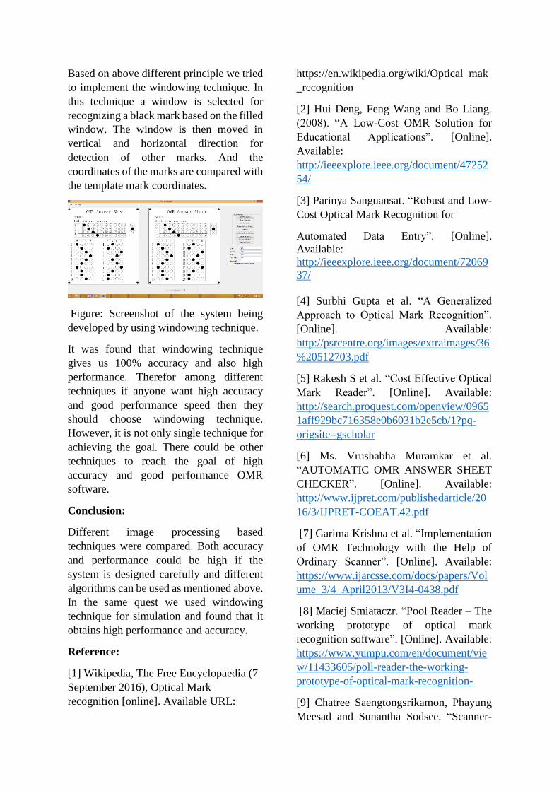
Based on above different principle we tried
to implement the windowing technique. In
this technique a window is selected for
recognizing a black mark based on the filled
window. The window is then moved in
vertical and horizontal direction for
detection of other marks. And the
coordinates of the marks are compared with
the template mark coordinates.
Figure: Screenshot of the system being
developed by using windowing technique.
It was found that windowing technique
gives us 100% accuracy and also high
performance. Therefor among different
techniques if anyone want high accuracy
and good performance speed then they
should choose windowing technique.
However, it is not only single technique for
achieving the goal. There could be other
techniques to reach the goal of high
accuracy and good performance OMR
software.
Conclusion:
Different image processing based
techniques were compared. Both accuracy
and performance could be high if the
system is designed carefully and different
algorithms can be used as mentioned above.
In the same quest we used windowing
technique for simulation and found that it
obtains high performance and accuracy.
Reference:
[1] Wikipedia, The Free Encyclopaedia (7
September 2016), Optical Mark
recognition [online]. Available URL:
https://en.wikipedia.org/wiki/Optical_mak
_recognition
[2] Hui Deng, Feng Wang and Bo Liang.
(2008). “A Low-Cost OMR Solution for
Educational Applications”. [Online].
Available:
http://ieeexplore.ieee.org/document/47252
54/
[3] Parinya Sanguansat. “Robust and Low-
Cost Optical Mark Recognition for
Automated Data Entry”. [Online].
Available:
http://ieeexplore.ieee.org/document/72069
37/
[4] Surbhi Gupta et al. “A Generalized
Approach to Optical Mark Recognition”.
[Online]. Available:
http://psrcentre.org/images/extraimages/36
%20512703.pdf
[5] Rakesh S et al. “Cost Effective Optical
Mark Reader”. [Online]. Available:
http://search.proquest.com/openview/0965
1aff929bc716358e0b6031b2e5cb/1?pq-
origsite=gscholar
[6] Ms. Vrushabha Muramkar et al.
“AUTOMATIC OMR ANSWER SHEET
CHECKER”. [Online]. Available:
http://www.ijpret.com/publishedarticle/20
16/3/IJPRET-COEAT.42.pdf
[7] Garima Krishna et al. “Implementation
of OMR Technology with the Help of
Ordinary Scanner”. [Online]. Available:
https://www.ijarcsse.com/docs/papers/Vol
ume_3/4_April2013/V3I4-0438.pdf
[8] Maciej Smiataczr. “Pool Reader – The
working prototype of optical mark
recognition software”. [Online]. Available:
https://www.yumpu.com/en/document/vie
w/11433605/poll-reader-the-working-
prototype-of-optical-mark-recognition-
[9] Chatree Saengtongsrikamon, Phayung
Meesad and Sunantha Sodsee. “Scanner-

Based Optical Mark Recognition”.
[Online]. Available:
https://www.researchgate.net/publication/2
64882235_Scanner-
Based_Optical_Mark_Recognition

Quantum Annealing:
A Case Study on Why Quantum Annealing is considered as An Optimized
Technique against Simulated Annealing
Aasish Kumar Sharma1, Pradip Maharjan2
Abstracts―The paper presents a case study on
Quantum Annealing in relation to Simulated
Annealing. At first it includes some details on
Annealing, Simulated Annealing and Quantum
Annealing techniques for solving problems where
search space is discrete. Onward, based on various
experimental results, conducted on quantum
annealing machine (e.g. D-Wave) in compare to
different classical approaches on variant
performance parameters shows why Quantum
Annealing is considered optimum technique than
Simulated Annealing.
Keywords―Quantum Annealing, Simulated
Annealing, discrete search space.
1. INTRODUCTION
The purpose of this paper is to escalate and evaluate
possible reasons and parameters mentioned in already
presented research findings related to Quantum
Annealing and Simulated Annealing which is a
mechanical metaheuristic (generic and approximate)
method to solve combinatorial optimization problems,
in order to highlight even optimum solutions. The paper
evaluates and compares different research findings
published in various public Medias related to the topic
and presents the analysis for supporting the method
with more optimum optimization method based on
performance parameters.
The paper consists of altogether 5 sections.
Section 1 includes introduction, section 2 covers most
of the basic definitions and algorithms related to the
paper content. Section 3 evaluates different
experiments and research papers found related to the
title and section 4 outlines the conclusion. Finally,
section 5 list out all references and their details.
2. FUNDAMENTAL DEFINITIONS
1 Author, M.E. (Computer ), Nepal College of Information Technology, [email protected] 2 Co-Author, M.E. (Computer ), Nepal College of Information Technology, [email protected]
Before jumping into the core analysis let us start with
some fundaments details. Like what does discrete
search space and annealing means as mentioned above
in the abstract?
2.1. Discrete Search Space:
Discrete Space means where space are broken up into
multiple states. Like in Travelling Sales Man Problem
different cities represents different states and the search
is to find the optimum path to travel all the cities ending
at the same city where it starts, in contrast to a
continuous path like in a maze [1].
2.2. Annealing:
In classical physics annealing is referred to a slow
cooling process of a molten metal object in order to
efficiently bring the metal into an optimum state of low-
energy in solid state. In this process at first a metal
object is heated to its melting point and then scheduled
to cool down slowly in a controlled environment. Here,
the temperature scheduled cooling plays a significant
role as an optimizer to overcome the energy barriers i.e.
the local minima(s) to get into global minima of the
metal energy distribution, enhancing the properties of
the metal. Despite, this is not the case if the heated metal
is cooled rapidly, that gets stuck at higher energy state
local maxima(s) making it more brittle and may have
bubbles and cracks [2]. This is also related to statistical
mechanics.
2.3. Statistical Mechanics:
It is a branch of modern physics related to the statistical
analysis of thermodynamic system having large number
of microscopic particles taken in unit volume. As it has
large sample range only the most probable
characteristics of the system at given temperature in
thermal equilibrium is known. It is mainly based on
microscopic physical laws and statistical probability
theories. In thermodynamics, energy state of a system
is equivalent to the energy state of each of the particles
constituting in it. The probability distribution relative to

the temperate of the system at one state to changed
energy state is given by
𝑃(𝐸𝑖 , 𝐸𝑖+1, 𝑇) = 𝑒(𝐸𝑖−𝐸𝑖+1 𝑘𝐵𝑇 )⁄ , (1)
Where P is the probability of, 𝐸𝑖 , 𝐸𝑖+1 (are the current
and next energy state), and T (is the instantaneous
temperature in Kelvin) where 𝑘𝐵 (is the Boltzmann’s
constant: 1.38× 10⁻²³ 𝐽 𝐾⁄ ).
This formula gives the probability of the change of
energy from one energy state to next energy state
depending on the change of temperature [3].
2.4. Combinatorial Optimization
Problems:
Related to computer science, this includes set of
discrete search space problems that are considered hard
to solve. Its aim is to find the cost function (the change
of energy) of the problem taken against variant(s) in
order to minimize or maximize the cost to reduce the
complexity. For example, in Travelling Salesman
Problem (TSP), a salesman starts from one city, travels
to all other cities and returns to the same city. For this
an optimum route is required, with minimum cost. So
the probabilities for all the route combinations are
evaluated and the path with optimum cost is selected
[3].
2.5. Monte Carlo Method (MC):
MC is an algorithm for finding stochastic (random)
probability distribution to estimate the probability of
occurrence of an event or state, given stationary
distribution with respect to the time or space. This
method is mainly used for problem classes like
generating patterns from probability distribution,
optimization and similar discrete space problems [4].
2.6. Markov Chain (MC):
This is a model that describes the probability of
occurrence of next event dependent on sequence of
previous event. The Markov Chain have to satisfy the
Markov Property named after Russian Mathematician
Andrey Markov. According to this property the future
state is predicted based on present state not on the
combination of sequence of the past states. Such a
process following Markov property is taken as Markov
process and the model as Markov Chain [4].
2.7. Markov Chain Monte Carlo
(MCMC) Algorithm:
The combination of Monte Carlo Algorithm and
Markov Chain is known as Markov Chain Monte Carlo
(MCMC) Algorithm. The modern version of the
MCMC method was invented in the late 1940s by
Stanislaw Ulam, while he was working on nuclear
weapon projects at the Los Alamos National
Laboratory. Immediately, after Ulam's breakthrough,
John von Neumann understood its importance and
programmed the ENIAC computer to carry out Monte
Carlo calculations [4].
2.8. Metropolis Algorithm:
This is based on MCMC method. Named after Nicholas
Metropolis, the algorithm helps to find random sample
sequence from probability distribution for the problems
that cannot be directly sampled. According to
Metropolis et al. [5], it provides an efficient algorithm
to simulate a collection of atoms in equilibrium at a
given temperature, by mainly working for two things:
one is to determine the cost function 𝑓(𝑠) of the
solution 𝑠 (i.e. also represented as ∆𝐸, the change in
energy) and the second is the probability of the cost
function i.e.
𝑃(∆𝐸) = 𝑒−∆𝐸 𝑘𝐵𝑇⁄ , (2)
Where 𝑘𝐵 is the Boltzmann’s constant: 1.38×
10−23 𝐽 𝐾⁄ and T is the temperature in Kelvin)
2.9. Simulated Annealing (SA):
SA is a nature inspired (of physics), stochastic
metaheuristics (some random rules are applied during
the search), single-solution based algorithms (where
the single solution gets evolved during the search) and
memoryless method [6]. SA is known from the work of
S. Kirkpatrick et al. [3] and V. Cerny [7], where it has
been applied for graph partitioning and VLSI design.
The algorithm they proposed is a derivation of
Metropolis Algorithm as a compact and robust
technique, which provides optimum solutions to
combinatorial search with a substantial reduction in
computation time. The idea is drawn from metallurgical
annealing process and statistical thermodynamics
or equilibrium i.e. statistical mechanics (as described
earlier in this section). It combines both “divide and
conquer” and “iterative improvement” strategies for
heuristics. The SA algorithm prescribed is as follows:
Algorithm 2.1 Template of simulated annealing
algorithm [6].
Input: Cooling Schedule
𝑠 = 𝑠0 ; /* Generation of the initial solution */
𝑇 = 𝑇𝑚𝑎𝑥 ; /* Starting temperature */
Repeat
Repeat /* At a fixed temperature */
Generate a random neighbor 𝑠′ ;
∆𝐸 = 𝑓(𝑠′) − 𝑓(𝑠) ;
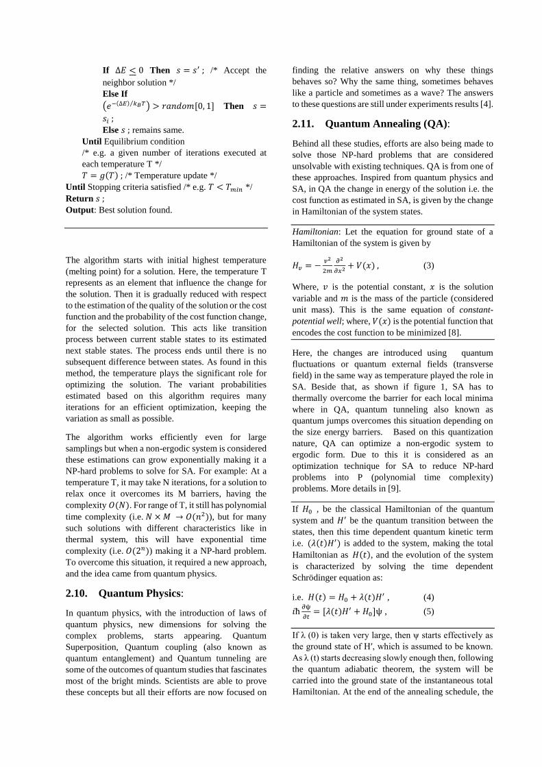
If ∆𝐸 < 0 Then 𝑠 = 𝑠′ ; /* Accept the
neighbor solution */
Else If
(𝑒−(∆𝐸) 𝑘𝐵𝑇⁄ ) > 𝑟𝑎𝑛𝑑𝑜𝑚[0, 1] Then 𝑠 =
𝑠𝑖 ;
Else 𝑠 ; remains same.
Until Equilibrium condition
/* e.g. a given number of iterations executed at
each temperature T */
𝑇 = 𝑔(𝑇) ; /* Temperature update */
Until Stopping criteria satisfied /* e.g. 𝑇 < 𝑇𝑚𝑖𝑛 */
Return 𝑠 ;
Output: Best solution found.
The algorithm starts with initial highest temperature
(melting point) for a solution. Here, the temperature T
represents as an element that influence the change for
the solution. Then it is gradually reduced with respect
to the estimation of the quality of the solution or the cost
function and the probability of the cost function change,
for the selected solution. This acts like transition
process between current stable states to its estimated
next stable states. The process ends until there is no
subsequent difference between states. As found in this
method, the temperature plays the significant role for
optimizing the solution. The variant probabilities
estimated based on this algorithm requires many
iterations for an efficient optimization, keeping the
variation as small as possible.
The algorithm works efficiently even for large
samplings but when a non-ergodic system is considered
these estimations can grow exponentially making it a
NP-hard problems to solve for SA. For example: At a
temperature T, it may take N iterations, for a solution to
relax once it overcomes its M barriers, having the
complexity 𝑂(𝑁). For range of T, it still has polynomial
time complexity (i.e. 𝑁 × 𝑀 → 𝑂(𝑛2)), but for many
such solutions with different characteristics like in
thermal system, this will have exponential time
complexity (i.e. 𝑂(2𝑛)) making it a NP-hard problem.
To overcome this situation, it required a new approach,
and the idea came from quantum physics.
2.10. Quantum Physics:
In quantum physics, with the introduction of laws of
quantum physics, new dimensions for solving the
complex problems, starts appearing. Quantum
Superposition, Quantum coupling (also known as
quantum entanglement) and Quantum tunneling are
some of the outcomes of quantum studies that fascinates
most of the bright minds. Scientists are able to prove
these concepts but all their efforts are now focused on
finding the relative answers on why these things
behaves so? Why the same thing, sometimes behaves
like a particle and sometimes as a wave? The answers
to these questions are still under experiments results [4].
2.11. Quantum Annealing (QA):
Behind all these studies, efforts are also being made to
solve those NP-hard problems that are considered
unsolvable with existing techniques. QA is from one of
these approaches. Inspired from quantum physics and
SA, in QA the change in energy of the solution i.e. the
cost function as estimated in SA, is given by the change
in Hamiltonian of the system states.
Hamiltonian: Let the equation for ground state of a
Hamiltonian of the system is given by
𝐻𝑣 = −𝑣2
2𝑚
𝜕2
𝜕𝑥2 + 𝑉(𝑥) , (3)
Where, 𝑣 is the potential constant, 𝑥 is the solution
variable and 𝑚 is the mass of the particle (considered
unit mass). This is the same equation of constant-
potential well; where, 𝑉(𝑥) is the potential function that
encodes the cost function to be minimized [8].
Here, the changes are introduced using quantum
fluctuations or quantum external fields (transverse
field) in the same way as temperature played the role in
SA. Beside that, as shown if figure 1, SA has to
thermally overcome the barrier for each local minima
where in QA, quantum tunneling also known as
quantum jumps overcomes this situation depending on
the size energy barriers. Based on this quantization
nature, QA can optimize a non-ergodic system to
ergodic form. Due to this it is considered as an
optimization technique for SA to reduce NP-hard
problems into P (polynomial time complexity)
problems. More details in [9].
If 𝐻0 , be the classical Hamiltonian of the quantum
system and 𝐻′ be the quantum transition between the
states, then this time dependent quantum kinetic term
i.e. (𝜆(𝑡)𝐻′) is added to the system, making the total
Hamiltonian as 𝐻(𝑡), and the evolution of the system
is characterized by solving the time dependent
Schrödinger equation as:
i.e. 𝐻(𝑡) = 𝐻0 + 𝜆(𝑡)𝐻′ , (4)
𝑖ћ𝜕ψ
𝜕𝑡= [𝜆(𝑡)𝐻′ + 𝐻0]ψ , (5)
If λ (0) is taken very large, then ψ starts effectively as
the ground state of H′, which is assumed to be known.
As λ (t) starts decreasing slowly enough then, following
the quantum adiabatic theorem, the system will be
carried into the ground state of the instantaneous total
Hamiltonian. At the end of the annealing schedule, the
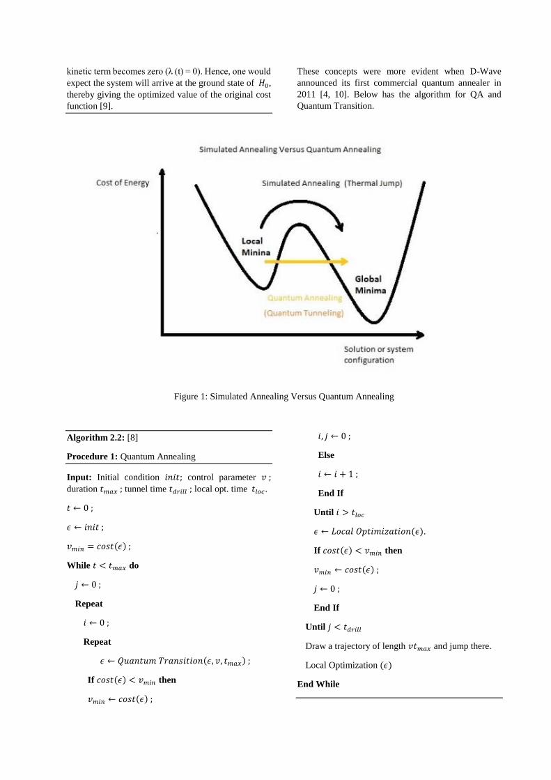
kinetic term becomes zero (λ (t) = 0). Hence, one would
expect the system will arrive at the ground state of 𝐻0,
thereby giving the optimized value of the original cost
function [9].
These concepts were more evident when D-Wave
announced its first commercial quantum annealer in
2011 [4, 10]. Below has the algorithm for QA and
Quantum Transition.
Figure 1: Simulated Annealing Versus Quantum Annealing
Algorithm 2.2: [8]
Procedure 1: Quantum Annealing
Input: Initial condition 𝑖𝑛𝑖𝑡; control parameter 𝑣 ;
duration 𝑡𝑚𝑎𝑥 ; tunnel time 𝑡𝑑𝑟𝑖𝑙𝑙 ; local opt. time 𝑡𝑙𝑜𝑐.
𝑡 ← 0 ;
𝜖 ← 𝑖𝑛𝑖𝑡 ;
𝑣𝑚𝑖𝑛 = 𝑐𝑜𝑠𝑡(𝜖) ;
While 𝑡 < 𝑡𝑚𝑎𝑥 do
𝑗 ← 0 ;
Repeat
𝑖 ← 0 ;
Repeat
𝜖 ← 𝑄𝑢𝑎𝑛𝑡𝑢𝑚 𝑇𝑟𝑎𝑛𝑠𝑖𝑡𝑖𝑜𝑛(𝜖, 𝑣, 𝑡𝑚𝑎𝑥) ;
If 𝑐𝑜𝑠𝑡(𝜖) < 𝑣𝑚𝑖𝑛 then
𝑣𝑚𝑖𝑛 ← 𝑐𝑜𝑠𝑡(𝜖) ;
𝑖, 𝑗 ← 0 ;
Else
𝑖 ← 𝑖 + 1 ;
End If
Until 𝑖 > 𝑡𝑙𝑜𝑐
𝜖 ← 𝐿𝑜𝑐𝑎𝑙 𝑂𝑝𝑡𝑖𝑚𝑖𝑧𝑎𝑡𝑖𝑜𝑛(𝜖).
If 𝑐𝑜𝑠𝑡(𝜖) < 𝑣𝑚𝑖𝑛 then
𝑣𝑚𝑖𝑛 ← 𝑐𝑜𝑠𝑡(𝜖) ;
𝑗 ← 0 ;
End If
Until 𝑗 < 𝑡𝑑𝑟𝑖𝑙𝑙
Draw a trajectory of length 𝑣𝑡𝑚𝑎𝑥 and jump there.
Local Optimization (𝜖)
End While

Procedure 2: Quantum Transitions
Input: Initial condition 𝜖 ; chain length 𝑣𝑡 ; set of
neighbors to estimate 𝑁 𝑒𝑖𝑔ℎ ;
For all neighbor 𝑘 ∈ 𝑁 𝑒𝑖𝑔ℎ do
Estimate the wave function ψ𝑣(𝑘) ;
End for
𝑏𝑒𝑠𝑡 ← select a neighbor in 𝑁 𝑒𝑖𝑔ℎ with probability
proportional to ψ𝑣
Return 𝑏𝑒𝑠𝑡
QA is followed by quantum transition for change in
quantum fluctuation.
3. EVALUATION: COMPARING QA
AND SA PUBLISHED WORKS
3.1. Reference Paper 1:
Nishimori et al., “Ground-state Statistics from
Annealing Algorithms: Quantum vs Classical
Approaches”, listed in Cornell University Library [11].
Kadowaki and Nishimori proposed about QA in 1998
as a quantum mechanical metaheuristic (generic and
approximate method) to solve combinatorial
optimization and sampling problems. Later the
Canadian Research Institute D-Wave System’s also
introduced its first commercial quantum annealer that
works on similar concepts [12].
Subject:
In this paper, Nishimori et al. has studied the
performance of QA against the systems with ground-
state degeneracy by:
a) Directly solving the Schrödinger equation for small
systems - Five-spin toy model and
b) Quantum Monte Carlo Simulations for larger
systems - Two-dimensional Villain fully-frustrated
Ising model.
Result:
The results shows that the quantum annealing is not
able to identify all degenerate ground-states though its
ground-state values are efficiently estimated. That is,
the method fails to find certain ground-state
configurations independent of the annealing rate.
Which is not the case with SA, where all the degenerate
states are reached with almost equal probability, if the
annealing rate of the temperature is sufficiently slow. A
great improvement to the quantum transitions to all
states with equal weight is seen in QA but this also takes
proportional annealing time. That is why, no speed gain
is mentioned. Therefore, the result concludes that QA is
superior to SA only when ground-state energy is
needed.
3.2. Reference Paper 2:
Chi Wang et al., “Quantum versus Simulated Annealing
in Wireless Interference Network Optimization”,
Published in Nature, Open scientific reports [13].
Subject:
The paper includes, application of D-Wave System’s
quantum annealing machine on a real-world application
in wireless networking. Targeting the scheduling of the
activation of the air-links for maximum throughput that
subject to interference avoidance near network nodes.
D-Wave (DW) quantum annealer implementation is
made error resistive by a Hamiltonian extra penalty
weight adjustment that enlarges the gap and
substantially reduces the occurrence of interference
violations resulting from inevitable spin bias and
coupling errors. The outcomes of experiment are
compared with classical annealing counter part SA.
Result:
QA benefits more than SA from gap expansion process
(process followed in this experiment), both in terms of
ST99 speedup and network queue occupancy. The
results are compared based on three matrices: actual
network performance, accuracy and speed and the
results are in the favor of QA.
3.3. Reference Paper 3:
Richard Y. Li et al., “Quantum annealing versus
classical machine learning applied to a simplified
computational biology problem”, is an open article
published in Nature, open article [14].
Subject:
The paper has applied study on quantum machine
learning approach to classify and rank binding affinities
using simplified data sets of a small number of DNA
sequences, derived from actual binding affinity
experiments. They trained commercially available D-
Wave quantum annealer (DW) to classify and rank
transcription factor binding. Transcription factors
regulate gene expression, but how these proteins linked
to their target DNA is unknown. The experiment is
compared with most of the classical approaches like
SA, SQA (Simulated Quantum Annealing), MLR
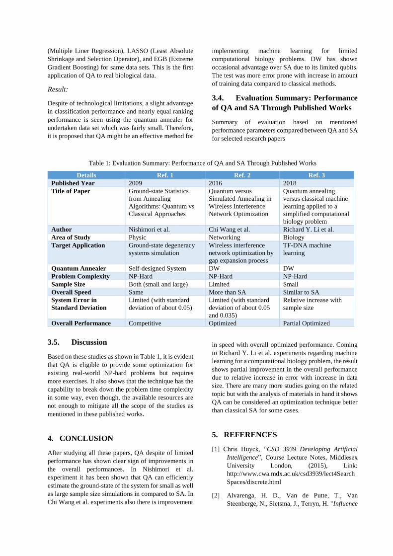
(Multiple Liner Regression), LASSO (Least Absolute
Shrinkage and Selection Operator), and EGB (Extreme
Gradient Boosting) for same data sets. This is the first
application of QA to real biological data.
Result:
Despite of technological limitations, a slight advantage
in classification performance and nearly equal ranking
performance is seen using the quantum annealer for
undertaken data set which was fairly small. Therefore,
it is proposed that QA might be an effective method for
implementing machine learning for limited
computational biology problems. DW has shown
occasional advantage over SA due to its limited qubits.
The test was more error prone with increase in amount
of training data compared to classical methods.
3.4. Evaluation Summary: Performance
of QA and SA Through Published Works
Summary of evaluation based on mentioned
performance parameters compared between QA and SA
for selected research papers
Table 1: Evaluation Summary: Performance of QA and SA Through Published Works
3.5. Discussion
Based on these studies as shown in Table 1, it is evident
that QA is eligible to provide some optimization for
existing real-world NP-hard problems but requires
more exercises. It also shows that the technique has the
capability to break down the problem time complexity
in some way, even though, the available resources are
not enough to mitigate all the scope of the studies as
mentioned in these published works.
4. CONCLUSION
After studying all these papers, QA despite of limited
performance has shown clear sign of improvements in
the overall performances. In Nishimori et al.
experiment it has been shown that QA can efficiently
estimate the ground-state of the system for small as well
as large sample size simulations in compared to SA. In
Chi Wang et al. experiments also there is improvement
in speed with overall optimized performance. Coming
to Richard Y. Li et al. experiments regarding machine
learning for a computational biology problem, the result
shows partial improvement in the overall performance
due to relative increase in error with increase in data
size. There are many more studies going on the related
topic but with the analysis of materials in hand it shows
QA can be considered an optimization technique better
than classical SA for some cases.
5. REFERENCES
[1] Chris Huyck, “CSD 3939 Developing Artificial
Intelligence”, Course Lecture Notes, Middlesex
University London, (2015), Link:
http://www.cwa.mdx.ac.uk/csd3939/lect4Search
Spaces/discrete.html
[2] Alvarenga, H. D., Van de Putte, T., Van
Steenberge, N., Sietsma, J., Terryn, H. "Influence
Details Ref. 1 Ref. 2 Ref. 3
Published Year 2009 2016 2018
Title of Paper Ground-state Statistics
from Annealing
Algorithms: Quantum vs
Classical Approaches
Quantum versus
Simulated Annealing in
Wireless Interference
Network Optimization
Quantum annealing
versus classical machine
learning applied to a
simplified computational
biology problem
Author Nishimori et al. Chi Wang et al. Richard Y. Li et al.
Area of Study Physic Networking Biology
Target Application Ground-state degeneracy
systems simulation
Wireless interference
network optimization by
gap expansion process
TF-DNA machine
learning
Quantum Annealer Self-designed System DW DW
Problem Complexity NP-Hard NP-Hard NP-Hard
Sample Size Both (small and large) Limited Small
Overall Speed Same More than SA Similar to SA
System Error in
Standard Deviation
Limited (with standard
deviation of about 0.05)
Limited (with standard
deviation of about 0.05
and 0.035)
Relative increase with
sample size
Overall Performance Competitive Optimized Partial Optimized
of Carbide Morphology and Microstructure on
the Kinetics of Superficial Decarburization of C-
Mn Steels", Metal Mater Trans A, (Apr 2009).
DOI: 10.1007/s11661-014-2600-y, Link:
http://rdcu.be/mFXR
[3] S. Kirkpatrick; C. D. Gelatt; M. P. Vecchi,
“Optimization by Simulated Annealing”, Science,
New Series, Vol. 220, No. 4598. (May 13, 1983),
pp. 671-680, Link:
https://pdfs.semanticscholar.org/beb2/1ee4a3721
484b5d2c7ad04e6babd8d67af1d.pdf
[4] Arnab Das, Bikas K. Chakrabarti, “Quantum
Annealing and Related Optimization Methods”,
Springer, Lect. Notes Phys. 679 (Springer, Berlin
Heidelberg 2005), DOI 10.1007/b135699, Link:
https://www.researchgate.net/publication/252247
914_Quantum_Annealing_and_Related_Optimiz
ation_Methods
[5] Nicholas Metropolis, Arianna W. Rosenbluth,
Marshall N. Rosenbluth, Augusta H. Teller, and
Edward Teller, “Equation of State Calculations
by Fast Computing Machines”, J. Chem. Phys. 21,
1087 (1953); DOI: 10.1063/1.1699114, Link:
https://bayes.wustl.edu/Manual/EquationOfState.
[6] El-Ghazali Talbi, “Metaheuristics From Design
To Implementation”, University of Lille – CNRS
– INRIA, Book, Published by John Wiley & Sons,
Inc., Hoboken, New Jersey, p. cm , (2009), ISBN
978-0-470-27858-1 (cloth), Link:
https://leseprobe.buch.de/images-
adb/65/c5/65c53443-f150-4d13-91c0-
285a7f28e8bd.pdf
[7] V. Cerny, “A thermodynamical approach to the
traveling salesman problem: An efficient
simulation algorithm”. Plenum Publishing
Corporation, Journal of Optimization Theory and
Applications, 45:41–51, (1985), DOI: 0022-
3239/85/0100-0041504.50/0 © 1985, Link:
http://www.webpages.uidaho.edu/~stevel/565/lit
erature/tsp.pdf
[8] Diego de Falco and Dario Tamascelli, “An
Introduction to Quantum Annealing”, RAIRO-
Theor. Inf. Appl. 45 99–116 (2011) DOI:
10.1051/ita/2011013, Link:
http://www.numdam.org/article/ITA_2011__45_
1_99_0.pdf
[9] Sudip Mukherjee, and Bikas K. Chakrabarti
"Multivariable Optimization: Quantum
Annealing & Computation", Eur. Phys. J. Special
Topics, 224 pp 17–24 (2015), DOI:
10.1140/epjst/e2015-02339-y, arXiv:
1408.3262, Link:
https://arxiv.org/pdf/1408.3262.pdf
[10] M. W. Johnson et al., "Quantum annealing with
manufactured spins", Nature, Letter, 473 194
(2011), DOI: 10.1038/nature10012, Link:
http://convexoptimization.com/TOOLS/manufact
uredspins.pdf
[11] Yoshiki Matsuda, Hidetoshi Nishimori and
Helmut G. Katzgraber, “Ground-state statistics
from annealing algorithms: Quantum vs classical
approaches”, Cornell University Library, quant-
ph (13 Jul 2009), arXiv: 0808.0365v3, Link:
https://arxiv.org/abs/0808.0365v3;
http://iopscience.iop.org/article/10.1088/1367-
2630/11/7/073021/pdf.
[12] Hidetoshi Nishimori, GCOE "Nanoscience and
Quantum Physics" Department of
Physics/Complementary site, Tokyo Tech,
(2015), Link:
http://www.stat.phys.titech.ac.jp/~nishimori/QA/
q-annealing_e.html
[13] Chi Wang, Huo Chen, and Edmond Jonckheere
“Quantum versus Simulated Annealing in
Wireless Interference Network Optimization”,
Nature, Scientific Reports 6:25797 (2016)05:16;
DOI: 10.1038/srep25797,
www.nature.com/scientificreports, Link:
https://www.ncbi.nlm.nih.gov/pmc/articles/PMC
4867427/
[14] Richard Y. Li, Rosa Di Felice, Remo Rohs and
Daniel A. Lidar, “Quantum annealing versus
classical machine learning applied to a simplified
computational biology problem”, Nature, npj
Quantum Information, (2018) 4:14; DOI:
10.1038/s41534-018-0060-8,
www.nature.com/npjqi, Link:
https://www.ncbi.nlm.nih.gov/pmc/articles/PMC
5891835/pdf/nihms947169.pdf

Theoretical Foundations of Computational Studies in Problem Solving Using
Mathematical Induction and Apagogical Argument
Abiral Sangroula
B.E. Computer Engineering
Nepal College of Information Technology
ABSTRACT
Computers are limited by space and
time. With the building concept of
theoretical foundations definition of both the
types of problems that can be solved using a
computer and the quality of their solutions
can be dictated. Theoretical
foundations required to study various sub-
disciplines in computer science. The actual
solution to a computational problem usually
lies outside these circumference, thus an
approximate solution must always be
computed. Topics included in the problem
solving with the concept of theoretical
foundations include propositional and
predicate logic with applications to logic
programming, database querying, and
program verification; and graph theory with
applications to analysis of algorithms; sets,
relations, and functions and their
applications in databases, functional
programming.
Keywords – Theoretical Foundations,
functional programming, logic
programming.
I. INTRODUCTION
In theoretical computational studies,
the theory of computation is the branch that
deals with how efficiently problems can be
solved on a model of computation, using
an algorithm. The field is divided into three
major branches: automata theory and
languages, computability theory,
and computational complexity theory, which
are linked by the question: "What are the
fundamental capabilities and limitations of
computers?".
In Theory of computability we study, which
problems can in principle be solved by
computers and how difficult the given
problem is. The difficulty is defined by quite
coarse level according to how difficult
model of computation is requires. In
addition theory of computability gives good
advice how to efficiently solve some special
type of problems.
In Theory of computational complexity we
study, how efficiently the problem can be
solved. Theory of computational complexity
reminds analysis of algorithms, but we don't
determine time and space complexity of an
individual algorithm, but the worst case
complexity class of the problem itself.
Theory of computational complexity gives
also good aids for reducing a problem into
other already known problems.
The Theory of Computation is also
concerned with finding the most efficient
methods for solving specific problems. This
is where the concept of problem solving
develops. For example, multiplying numbers
can be done more efficient than via the
simple method learned in elementary school.
The nature of efficient computation (and
computation in general) is indeed the
formative question of the Theory of

Computation. We consider this question (or
rather a cluster of questions) to be one of the
most fundamental scientific questions ever
asked. Unfortunately, the fundamental status
of this question is usually disregarded due to
its immediate technological impact.
Moreover, research in theory of computation
has been extremely successful and
productive in the few decades of its
existence, with continuously growing
momentum. This research has
revolutionized the understanding of
computation and has deep scientific and
philosophical consequences, which will be
further recognized in the future. Moreover,
this research and its dissemination through
education and interaction have been
responsible for enormous technological
progress.
II. RELATED WORKS
Lenore Blum, in his paper “Alan Turing and
the Other Theory of Computation
(expanded)”, has explained how Alan
Turing‟s work has been recognized in the
foundations of numerical computation, its
influence in modern complexity theory, and
how it helps provide a unifying concept for
the two major traditions of the theory of
computation.
Naimul Ferdous, has described the Program
for Turing Machine capable of recognizing
the language 1^n0^n, where n>0. He has
made state diagrams and has used the C
programming language to code the whole
program and has been successful to
determine if the number given is accepted to
be turing machine compatible or not.
Oded Goldreich and Avi Wigderson, have
summarized the main topics in Theoretical
foundations in scientific researches to
provide an assessment of the Theory of
Computing (TOC), as a fundamental
scientific discipline, highlighting the seeks
to understand computational phenomena, be
it natural, man-made or imaginative.
Lawrence S. Moss, in his paper entitled
“Connections of co algebra and semantic
modeling” has presented the area of co
algebra to people interested in the kinds of
semantic modeling that is prominent at
TARK. Co algebra is a general study of a
great many kinds of models, and these
include type spaces and Kripke models, and
many others.
Naimul Ferdous, has described the Program
for Pushdown automata (PDA) capable of
recognizing the language w#w belongs to R
where w {0, 1}* and∑={0,1,#}where n>0.
Similarly, he has also described the program
for deterministic finite automata (DFA) for
the implementation of string pattern ab*cb*
with the use of state diagrams and C-
programming language.
Margaret Archibald, has addressed all
aspects of infinity in automata theory, logic,
computability and verification and focus on
topics such as automata on infinite objects;
combinatorics, cryptography and
complexity; computability and complexity
on the real numbers; infinite games and their
connections to logic; logic, computability,
and complexity in finitely presentable
infinite structures; randomness and
computability; transfinite computation; and
verification of infinite state systems.
J. Aspnes, D.K. Goldenberg, A. S. Morse,
W. Whiteley, Y. R. Yang, B. D. O.
Anderson, P. N. Belhumeur provide a
theoretical foundation for the problem of
network localization in which some nodes
know their locations and other nodes
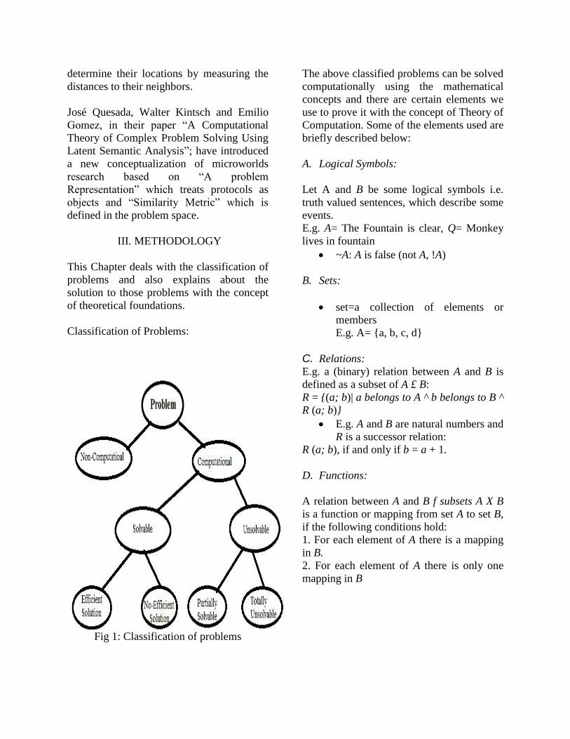
determine their locations by measuring the
distances to their neighbors.
José Quesada, Walter Kintsch and Emilio
Gomez, in their paper “A Computational
Theory of Complex Problem Solving Using
Latent Semantic Analysis”; have introduced
a new conceptualization of microworlds
research based on “A problem
Representation” which treats protocols as
objects and “Similarity Metric” which is
defined in the problem space.
III. METHODOLOGY
This Chapter deals with the classification of
problems and also explains about the
solution to those problems with the concept
of theoretical foundations.
Classification of Problems:
Fig 1: Classification of problems
The above classified problems can be solved
computationally using the mathematical
concepts and there are certain elements we
use to prove it with the concept of Theory of
Computation. Some of the elements used are
briefly described below:
A. Logical Symbols:
Let A and B be some logical symbols i.e.
truth valued sentences, which describe some
events.
E.g. A= The Fountain is clear, Q= Monkey
lives in fountain
~A: A is false (not A, !A)
B. Sets:
set=a collection of elements or
members
E.g. A= {a, b, c, d}
C. Relations: E.g. a (binary) relation between A and B is
defined as a subset of A £ B:
R = {(a; b)| a belongs to A ^ b belongs to B ^
R (a; b)}
E.g. A and B are natural numbers and
R is a successor relation:
R (a; b), if and only if b = a + 1.
D. Functions:
A relation between A and B f subsets A X B
is a function or mapping from set A to set B,
if the following conditions hold:
1. For each element of A there is a mapping
in B.
2. For each element of A there is only one
mapping in B

Figure 2: A=definition set, B=goal set, f
(A) = value set
Here, y = f(x) where (x; y) belongs to f:
E. Countability:
Set A is countable, if
1. A is finite or
2. There exists a bijection f : N→ A, for
which
A = {f (n)| n 2 belongs to N}
F. Proofing Methods:
Proving the problem statements using the
elements using has two basic methods which
are classified into the Mathematical
Induction and the other one is the
Undirected Proof. Both of them are
explained below:
MATHEMATICAL INDUCTION
Mathematical Induction is a „mathematical
proof‟ technique. Proving an infinite
sequence of statements is necessary for
proof by induction, a rigorous form of
deductive learning. It is essentially used to
prove in cases such as to prove that a
property P (n) holds for every prime
numbers n, i.e. for n= 2,3,5,7… and so on.
Symbols and Metaphors can be informally
used to understand the concept of
mathematical induction, such as the
metaphor of falling dominoes or climbing a
ladder.
Let us suppose that the Logical Function P
(n) holds true for all natural numbers. To
prove this statement we usually have two
parts to solve:
Case 1: When we keep n as null, i.e. n=0, P
(0) is true.
Case 2: The very next is the induction step.
That is, here we prove that for all n; P(n)
→P(n+1).
The example for mathematical induction is
given down below:
E.g.∑
For all n>=0
We get two conditions with the above
mentioned equation.
Condition 1: When n=0;
∑
Condition 2: Induction assumption;
€k belongs to N such that the claim holds
for all n <=k.
n=k+1:∑
∑
. So,
∑
+ (k + 1).
∑
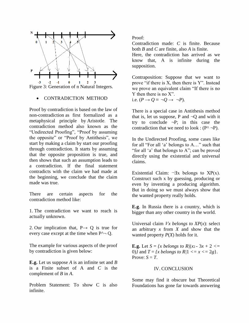
Figure 3: Generation of n Natural Integers.
CONTRADICTION METHOD
Proof by contradiction is based on the law of
non-contradiction as first formalized as a
metaphysical principle by Aristotle. The
contradiction method also known as the
“Undirected Proofing”, “Proof by assuming
the opposite” or “Proof by Antithesis”, we
start by making a claim by start our proofing
through contradiction. It starts by assuming
that the opposite proposition is true, and
then shows that such an assumption leads to
a contradiction. If the final statement
contradicts with the claim we had made at
the beginning, we conclude that the claim
made was true.
There are certain aspects for the
contradiction method like:
1. The contradiction we want to reach is
actually unknown.
2. Our implication that, P→ Q is true for
every case except at the time when P^¬ Q.
The example for various aspects of the proof
by contradiction is given below:
E.g. Let us suppose A is an infinite set and B
is a Finite subset of A and C is the
complement of B in A.
Problem Statement: To show C is also
infinite.
Proof:
Contradiction made: C is finite. Because
both B and C are finite, also A is finite.
Here, the contradiction has arrived as we
know that, A is infinite during the
supposition.
Contraposition: Suppose that we want to
prove “if there is X, then there is Y”. Instead
we prove an equivalent claim “If there is no
Y then there is no X”.
i.e. (P → Q ≡ ¬Q → ¬P).
There is a special case in Antithesis method
that is, let us suppose, P and ¬Q and with it
try to conclude ¬P; in this case the
contradiction that we need to look : (P^ ¬P).
In the Undirected Proofing, some cases like
for all “For all „a‟ belongs to A…” such that
“for all „a‟ that belongs to A”; can be proved
directly using the existential and universal
claims.
Existential Claim: ¬Ǝx belongs to XP(x).
Construct such x by guessing, producing or
even by inventing a producing algorithm.
But in doing so we must always show that
the wanted property really holds.
E.g. In Russia there is a country, which is
bigger than any other country in the world.
Universal claim Ѵx belongs to XP(x): select
an arbitrary x from X and show that the
wanted property P(X) holds for it.
E.g. Let S = {x belongs to R|(x2 - 3x + 2 <=
0)} and T = {x belongs to R|1 <= x <= 2g}.
Prove: S = T.
IV. CONCLUSION
Some may find it obscure but Theoretical
Foundations has gone far towards answering

the question of what problems can be solved
and which ones cannot. The theory of
computation provides the basis for creating
“correct models” of computational tools:
software, digital circuits, concurrent systems
etc. For instance, automata theory has been
used for in building compilers and abstract
machines. A sound understanding of theory
of computation is critical for understanding
of different algorithms.
Mathematical Induction method can be
extended to prove statements about more
general well-founded structures such as
trees. It in some form is the foundation of all
correctness proofs for computer programs.
Mathematical Induction is an inference rule
used in formal proofs; and are, in fact,
examples of deductive reasoning.
An existence proof by contradiction assumes
that some object doesn't exist, and then
proves that this would lead to a
contradiction; thus, such an object must
exist. Although it is quite freely used in
mathematical proofs, not every school of
mathematical thought accepts this kind
of non-constructive proof as universally
valid.
REFERENCES
1. Oded Goldreich, “A Brief Introduction
to the Theory of Computation”
(Available at
http://www.wisdom.weizmann.ac.il/~od
ed/toc-bi.html)
2. Oded Goldreich and Avi Wigderson,
“Theory of Computation: A Scientific
Perspective.” (Available at
http://www.wisdom.weizmann.ac.il/~od
ed/toc-sp2.html)
3. Michael Sipser, “Introduction to theory
of computation” (Available at:
https://theswissbay.ch/pdf/Book/Introdu
ction%20to%20the%20theory%20of%2
0computation_third%20edition%20-
%20Michael%20Sipser.pdf)
4. J. Aspnes, D.K. Goldenberg, A. S.
Morse, W. Whiteley, Y. R. Yang, B. D.
O. Anderson, P. N. Belhumeur, “A
theory of network Localization” : IEEE
Transactions on Mobile
Computing ( Volume: 5 , Issue: 12 , Dec.
2006 )
5. Lawrence S. Moss, “Connections of Co-
Algebra and Semantic Modeling”,
Department of Mathematics, Indiana
University.
6. A brief concept on Mathematical
induction is (Available at:
https://en.wikipedia.org/wiki/Mathemati
cal_induction)
7. “Sequence of Mathematical
Statements”, (Available at:
https://courses.lumenlearning.com/boun
dless-algebra/chapter/mathematical-
inductions/)
8. A brief concept on Proof by
Contradiction is (Available at:
https://en.wikipedia.org/wiki/Proof_by_c
ontradiction)

Image Steganography for Secure Message Transmission
Using Modified Hash LSB Technique and Twofish
Cryptographic Algorithm
Anish Bhattarai
Department of Computer Engineering
NCIT, Pokhara University
Kathmandu, Nepal
+977-9841822155
Dr. Sanjeeb Prasad Panday
Dept. of Comp. Science and Engineering
IoE, Pulchowk Campus, Tribhuvan University
Kathmandu, Nepal
Abstract—Cryptographic algorithm secures
message transmission over an open channel by
scrambling the plain message with the help of a
secret key, producing the cipher text. Intruders can
get this scrambled message and tries to decrypt it
and get the original message from it. Steganography
hides the message inside digital media such that
intruders does not know about the message
transmission and removes his/her attention. The
combination of both provides another layer of
security, thus preventing the opportunity to work on
the encrypted data for an intruder. This makes the
transmission of message highly secure than using
each separately. This paper is focused on combining
both cryptography and image steganography for
highly secure message transmission. The message is
encrypted using twofish encryption method with key
length of 256 bits. This encrypted message is then
embedded inside the RGB component of the pixel of
the cover image using modified Hash LSB (HLSB)
in (3, 2, 3) format producing stego image which is
now ready to send over an open channel. After the
implementation, MSE, PSNR, SSIM and KL
Divergence (Relative Entropy) are calculated. The
results show high security and greater similarity
between cover image and stego image, making our
system robust.
Keywords: Steganography; Cryptography;
Modified Hash LSB; Twofish Encryption
I. INTRODUCTION
Cryptography is the technique of scrambling and
changing text using a key, such that no one except the
key holders can get the message. This is the study of
technique with mathematical algorithm that goes in one
way but is very hard to get reverse in the similar way. It
is used for communication in today's world. From years
ago many algorithm has been proposed and used and
with the breaking of each of them / finding the
backdoor, each time new algorithms are being
proposed. Although todays Advanced Encryption
Standard (AES), is known to be secure but the cipher
are still openly accessed to intruders which doubts on
the security technology. Attacks are always being going
on but no cipher is broken to get the original message.
We are totally dependent upon and our information is
totally secure by the cryptographic algorithm. Our
information is secure for us, as we think but may not
appear to be. Cryptography never hides the cipher
which may create a problem regarding security. It says
to protect our confidentiality, integrity and
authentication but with such open environment it still
possess a risk.
So information hiding seems very important, this
can be achieved by using the steganography, it hides
information into its bits that is less affective to its visual
perception. This hides the information and doesn't
attract the attention of unintended people. Seems simple
but still a very powerful method to hide and protect our
data when used along with cryptography. Different
substitutions based of pixel difference, simple Least
Significant Bit (LSB) substitution, substitution in edge/
smooth areas are used, to solve the problem of capacity,
quality. With not giving the chance to know our data to
intruders to work on with, we can feel safe in the
context of security, confidentiality and authentication.
S. Mittal, S. Arora and R. Jain used RSA for
message encryption [1] to get the cipher text and hide it
using Simple LSB, they said that it can be used when
secrecy is preferred over power of bulk data
transmission. In hybrid approach of image
steganography by D. Kaur H. K. Verma and R. K.
Singh, they used X-OR operation to get the new cipher
text of a message text and this cipher text was
compressed using LZW compression scheme. This
increased the hiding capacity by reducing the size of
secret data. The data hiding capacity was 4.71 times
greater than traditional LSB method. But the PSNR was

less than the LSB method.
K. Joshi and R. Yadav used LSB with Shifting for
hiding the encrypted message [18], where message was
encrypted using Vernam Cipher algorithm. It uses
simple LSB, where message bits was hidden 1 bit per
pixel in grayscale image with 1 bit left circular shifting
operation carried out in the 4 LSB of cover Image and
the resultant is XORed with the message bit. Now this
resultant message bit after shifting followed by XOR
operation is then concealed in the LSB of cover Image.
It although gave good result and improved security over
simple LSB method but the problem was with the
hiding capacity, which was just a single bit per pixel for
grayscale image, which was very low.
Using Hash-LSB, M. H. Abood proposed the image
cryptography with RC4 [6] and Pixel shuffling, where
the image was encrypted using the RC4 stream cipher
algorithm and then pixel shuffling was done. Hash-LSB
was used to find the position of a bit inside the pixel of
cover image. It used the position of the concealed
picture pixels. The embedding process here used 3, 3, 2
LSB pattern. Here only Grayscale image was encrypted
and hidden into RGB image. The Hash-LSB technique
embeds secret grayscale image pixel bits into the RGB
image into 3 LSB of R, 3 LSB of G and 2 LSB of B.
The embed position of each pixel (8-bit) of secret image
in the LSB (red, green, blue) of cover image is
represented by p, where p is LSB bit position per pixel
and it is dependent upon static value of pixel number as
shown in equation (1). Let us suppose the grayscale
value of secret image pixel is 245. Its binary value is
11110101. Bits to be hidden in R is 111, in G is 101 and
in B is 01. Now bit position where bits can be hidden, k
is given by formula in (1).
P = H % L (1)
Where, P is the position of bit, from where we can start
to hide bits.
H is the position of any hidden picture pixel.
L is the total number of bits substitution in each
component pixel, which is 4 in case of Hash-LSB
technique.
If R, G, B of cover image is (11010100, 11100010,
10001001) and the value of P is 1 then, new R, G, B
would be (11011110, 11100111, 10001001). This cause
the secret image bit to be inserted inside the cover
pixel’s 4th LSB. The distortion caused due to this bit
alone is -8 to +8.
II. PROPOSED METHODOLOGY
Our methodology uses the combination of both
cryptography and steganography (cryptography
followed by steganography), to provide the security
through the message scrambling along with hiding the
scrambled/encrypted message, thus achieving the
greater level of data integrity, confidentiality and
security, than obtained if both are used separately. We
have used twofish encryption method for message
encryption followed by Modified Hash-LSB
Steganography method. The use of twofish encryption
strengthens the message security and also large
message can be encrypted by it easily unlike RSA [1]
or any other stream cipher where large message
encryption is a pain. Twofish with key length of 256
bits is used as its performance is better in term of speed
than other AES candidates for same key size [15]. The
proposed modified Hash-LSB method embed the
encrypted message bits into the component of a pixel
(R, G, B) in 3, 2, 3 format as the value of luminance of
an image is heavily dependent upon the value of green
pixel. The resultant stego image is send over the open
channel, the receiver first decodes the message bits to
get the cipher text and then uses the secret key to
decrypt the message and get the original plain message.
This prevents steganalayst to easily get the plain text
easily through random iterations to find the pattern.
A. Modified Hash-LSB
Modified Hash-LSB method uses the formula of
Hash-LSB method [6] as given in (1), but in different
way, such that it never touches the 4th LSB bit. As the
Hash-LSB was touching and altering the 4th bit, the
effect due to its change alone ranges from +8 to -8,
while in our method we removed that such that we are
only changing only upto 3rd LSB. The effect of
changing all three LSB itself ranges from +7 to -7,
which is less than changing 4th bit alone. From (1)
P = H % L
Where, the value of L is 3 in our case and H is
obtained dynamically from the 4 MSBs of R, G, B
component of a pixel of cover image / stego image.
Depending upon the value of position p for each
component (R, G, B) of a pixel, the message bits (3, 2,
3) are inserted in the pixel starting from that position in
clockwise direction.
Let us suppose message bits be 11110101. Let R, G,
B of cover image be (11010100, 11100010, 10001001).
Then 4 MSB of R, G, B is (1101, 1110, 1000) which is
decimal equivalent to (13, 14, 8).
Using P = H % L where L is 3 in our case.
The value of P is 1 for R and 2 for G, and 2 for B
then, new R, G, B would be (11010111, 11100001,
10001110). This cause the secret image bit to be
inserted inside the cover pixel within 3rd LSB. The
distortion caused due to this bit alone is -8 to +8.
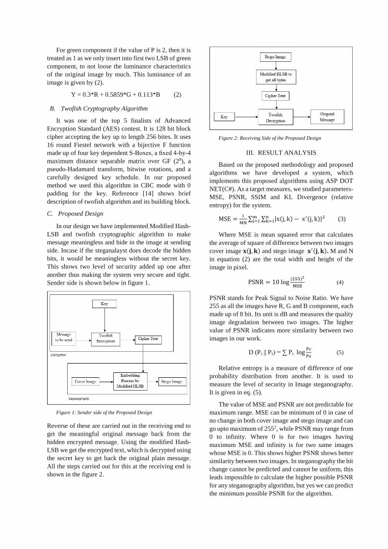
For green component if the value of P is 2, then it is
treated as 1 as we only insert into first two LSB of green
component, to not loose the luminance characteristics
of the original image by much. This luminance of an
image is given by (2).
Y = 0.3*R + 0.5859*G + 0.113*B (2)
B. Twofish Cryptography Algorithm
It was one of the top 5 finalists of Advanced
Encryption Standard (AES) contest. It is 128 bit block
cipher accepting the key up to length 256 bites. It uses
16 round Fiestel network with a bijective F function
made up of four key dependent S-Boxes, a fixed 4-by-4
maximum distance separable matrix over GF (28), a
pseudo-Hadamard transform, bitwise rotations, and a
carefully designed key schedule. In our proposed
method we used this algorithm in CBC mode with 0
padding for the key. Reference [14] shows brief
description of twofish algorithm and its building block.
C. Proposed Design
In our design we have implemented Modified Hash-
LSB and twofish cryptographic algorithm to make
message meaningless and hide in the image at sending
side. Incase if the steganalayst does decode the hidden
bits, it would be meaningless without the secret key.
This shows two level of security added up one after
another thus making the system very secure and tight.
Sender side is shown below in figure 1.
Figure 1: Sender side of the Proposed Design
Reverse of these are carried out in the receiving end to
get the meaningful original message back from the
hidden encrypted message. Using the modified Hash-
LSB we get the encrypted text, which is decrypted using
the secret key to get back the original plain message.
All the steps carried out for this at the receiving end is
shown in the figure 2.
Figure 2: Receiving Side of the Proposed Design
III. RESULT ANALYSIS
Based on the proposed methodology and proposed
algorithms we have developed a system, which
implements this proposed algorithms using ASP DOT
NET(C#). As a target measures, we studied parameters-
MSE, PSNR, SSIM and KL Divergence (relative
entropy) for the system.
MSE =1
MN∑ ∑ |x(j, k) − x′(j, k)|2n
k=1mj=1 (3)
Where MSE is mean squared error that calculates
the average of square of difference between two images
cover image 𝐱(𝐣, 𝐤) and stego image 𝐱′(𝐣, 𝐤). M and N
in equation (2) are the total width and height of the
image in pixel.
PSNR = 10 log(255)2
MSE (4)
PSNR stands for Peak Signal to Noise Ratio. We have
255 as all the images have R, G and B component, each
made up of 8 bit. Its unit is dB and measures the quality
image degradation between two images. The higher
value of PSNR indicates more similarity between two
images in our work.
D (Pc || Ps) = ∑ Pc logPc
Ps (5)
Relative entropy is a measure of difference of one
probability distribution from another. It is used to
measure the level of security in Image steganography.
It is given in eq. (5).
The value of MSE and PSNR are not predictable for
maximum range. MSE can be minimum of 0 in case of
no change in both cover image and stego image and can
go upto maximum of 2552, while PSNR may range from
0 to infinity. Where 0 is for two images having
maximum MSE and infinity is for two same images
whose MSE is 0. This shows higher PSNR shows better
similarity between two images. In steganography the bit
change cannot be predicted and cannot be uniform, this
leads impossible to calculate the higher possible PSNR
for any steganography algorithm, but yes we can predict
the minimum possible PSNR for the algorithm.

In Hash-LSB we have calculated the minimum
possible PSNR as we always get any of the four
possible options (embedded anticlockwise) to hide text
using this algorithm and compared with our modified
Hash-LSB algorithm.
TABLE I: MSE for all possible positions p in HLSB
P Change in
(R,G,B) value (Yc Ys) MSE = (Yc Ys)2
0 (14,13,3) 12.1557 147.761
1 (7,14,9) 11.2066 125.5878
2 (11,7,12) 8.7573 76.6903
3 (13,11,6) 11.0229 121.5043
Where (Yc Ys) is the luminance difference between
cover image and stego image.
At minimum MSE,
When MSE = 76.6903
PSNR = 10 log(255)2
76.69
= 29.28 dB
In our proposed modified case the change is always
limited to (R, G, B) change by (7, 3, 7) as we only alter
3 Red, 2 Green and 3 Blue LSBs.
Thus,
(Yc - Ys) = 0.3*7 + 0.5859 * 3 + 0.113 * 7 = 4.6487
MSE = (Yc Ys)2 = 21.60
PSNR = 10 log(255)2
21.60
= 34.78 dB
This clearly shows that the minimum PSNR is better for
Modified HLSB as compared to HLSB method.
RGB Cover Images used in our test
1 2 3
4 5
Stego Image for above cover Image
1 2 3
4 5
Cover images 1, 2, 3 and 4 are 256×256 pixels
images while image 5 is 210×150 pixels image. Using
the proposed method, message of different length are
embedded into above cover images. The length of
embedded messages are shown in the table II.
The timing parameters are also measured for our
different findings. All the parameters were found based
upon the average time taken for embedding and
extracting with 10 iterations. All these timing
parameters are shown in the table III.
TABLE II: Message length, MSE and PSNR calculations of
different stego images
Images Message Length MSE PSNR
1 237 bytes 0.007181 69.5687dB
2 1532 bytes 0.046798 61.4284dB
3 539 bytes 0.018858 65.3756dB
4 323 bytes 0.010181 68.0528dB
5 9162 bytes 0.50552 51.0934dB
TABLE III: Time taken for embedding and extracting message
Images Time to embed Time to extract
1 183.355 ms 81.134 ms
2 206.324 ms 99.338 ms
3 185.296 ms 93.726 ms
4 183.828 ms 89.732 ms
5 982.337 ms 195.344 ms
TABLE IV: SSIM and KL Divergence of pixel component
Images SSIM DR(Pc||Ps) DG(Pc||Ps) DB(Pc||Ps)
1 0.9998 0.00001170 0.00000827 0.00000997
2 0.9999 0.00003236 0.00002307 0.00003371
3 0.9988 0.00049879 0.00034917 0.00043749
4 0.9998 0.00000701 0.00003425 0.00005581
5 0.9999 0.00001309 0.00001637 0.00001566
6 0.9991 0.00002625 0.00001627 0.00002093
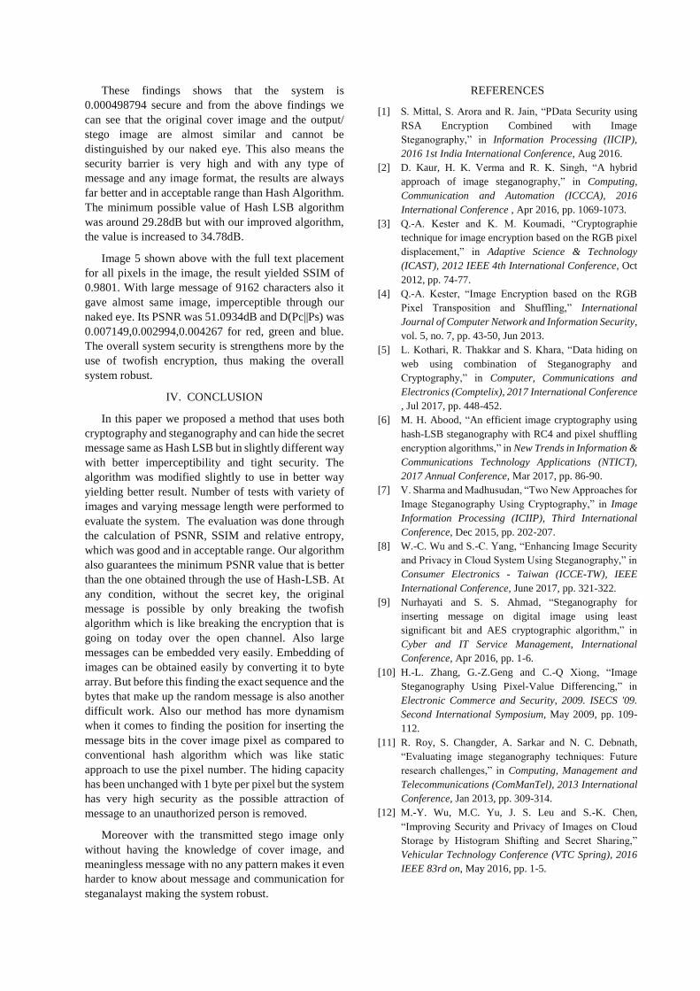
These findings shows that the system is
0.000498794 secure and from the above findings we
can see that the original cover image and the output/
stego image are almost similar and cannot be
distinguished by our naked eye. This also means the
security barrier is very high and with any type of
message and any image format, the results are always
far better and in acceptable range than Hash Algorithm.
The minimum possible value of Hash LSB algorithm
was around 29.28dB but with our improved algorithm,
the value is increased to 34.78dB.
Image 5 shown above with the full text placement
for all pixels in the image, the result yielded SSIM of
0.9801. With large message of 9162 characters also it
gave almost same image, imperceptible through our
naked eye. Its PSNR was 51.0934dB and D(Pc||Ps) was
0.007149,0.002994,0.004267 for red, green and blue.
The overall system security is strengthens more by the
use of twofish encryption, thus making the overall
system robust.
IV. CONCLUSION
In this paper we proposed a method that uses both
cryptography and steganography and can hide the secret
message same as Hash LSB but in slightly different way
with better imperceptibility and tight security. The
algorithm was modified slightly to use in better way
yielding better result. Number of tests with variety of
images and varying message length were performed to
evaluate the system. The evaluation was done through
the calculation of PSNR, SSIM and relative entropy,
which was good and in acceptable range. Our algorithm
also guarantees the minimum PSNR value that is better
than the one obtained through the use of Hash-LSB. At
any condition, without the secret key, the original
message is possible by only breaking the twofish
algorithm which is like breaking the encryption that is
going on today over the open channel. Also large
messages can be embedded very easily. Embedding of
images can be obtained easily by converting it to byte
array. But before this finding the exact sequence and the
bytes that make up the random message is also another
difficult work. Also our method has more dynamism
when it comes to finding the position for inserting the
message bits in the cover image pixel as compared to
conventional hash algorithm which was like static
approach to use the pixel number. The hiding capacity
has been unchanged with 1 byte per pixel but the system
has very high security as the possible attraction of
message to an unauthorized person is removed.
Moreover with the transmitted stego image only
without having the knowledge of cover image, and
meaningless message with no any pattern makes it even
harder to know about message and communication for
steganalayst making the system robust.
REFERENCES
[1] S. Mittal, S. Arora and R. Jain, “PData Security using
RSA Encryption Combined with Image
Steganography,” in Information Processing (IICIP),
2016 1st India International Conference, Aug 2016.
[2] D. Kaur, H. K. Verma and R. K. Singh, “A hybrid
approach of image steganography,” in Computing,
Communication and Automation (ICCCA), 2016
International Conference , Apr 2016, pp. 1069-1073.
[3] Q.-A. Kester and K. M. Koumadi, “Cryptographie
technique for image encryption based on the RGB pixel
displacement,” in Adaptive Science & Technology
(ICAST), 2012 IEEE 4th International Conference, Oct
2012, pp. 74-77.
[4] Q.-A. Kester, “Image Encryption based on the RGB
Pixel Transposition and Shuffling,” International
Journal of Computer Network and Information Security,
vol. 5, no. 7, pp. 43-50, Jun 2013.
[5] L. Kothari, R. Thakkar and S. Khara, “Data hiding on
web using combination of Steganography and
Cryptography,” in Computer, Communications and
Electronics (Comptelix), 2017 International Conference
, Jul 2017, pp. 448-452.
[6] M. H. Abood, “An efficient image cryptography using
hash-LSB steganography with RC4 and pixel shuffling
encryption algorithms,” in New Trends in Information &
Communications Technology Applications (NTICT),
2017 Annual Conference, Mar 2017, pp. 86-90.
[7] V. Sharma and Madhusudan, “Two New Approaches for
Image Steganography Using Cryptography,” in Image
Information Processing (ICIIP), Third International
Conference, Dec 2015, pp. 202-207.
[8] W.-C. Wu and S.-C. Yang, “Enhancing Image Security
and Privacy in Cloud System Using Steganography,” in
Consumer Electronics - Taiwan (ICCE-TW), IEEE
International Conference, June 2017, pp. 321-322.
[9] Nurhayati and S. S. Ahmad, “Steganography for
inserting message on digital image using least
significant bit and AES cryptographic algorithm,” in
Cyber and IT Service Management, International
Conference, Apr 2016, pp. 1-6.
[10] H.-L. Zhang, G.-Z.Geng and C.-Q Xiong, “Image
Steganography Using Pixel-Value Differencing,” in
Electronic Commerce and Security, 2009. ISECS '09.
Second International Symposium, May 2009, pp. 109-
112.
[11] R. Roy, S. Changder, A. Sarkar and N. C. Debnath,
“Evaluating image steganography techniques: Future
research challenges,” in Computing, Management and
Telecommunications (ComManTel), 2013 International
Conference, Jan 2013, pp. 309-314.
[12] M.-Y. Wu, M.C. Yu, J. S. Leu and S.-K. Chen,
“Improving Security and Privacy of Images on Cloud
Storage by Histogram Shifting and Secret Sharing,”
Vehicular Technology Conference (VTC Spring), 2016
IEEE 83rd on, May 2016, pp. 1-5.
[13] R. Halder, S. Sengupta, S. Ghosh and D. Kundu, “A
Secure Image Steganography Based on RSA Algorithm
and Hash-LSB Technique,” IOSR Journal of Computer
Engineering (IOSR-JCE), vol. 18, pp. 39-43,Jan – Feb.
2016.
[14] Schneier on Security - The Twofish Encryption
Algorithm. (December 2018) Retrieved from
https://www.schneier.com/academic/archives/1998/12/t
he_twofish_encrypti.html on 20 Nov 2018.
[15] B. Schneier and D. Whiting, “A Performance
Comparison of the Five AES Finalists”, in Proceedings
of the Third AES Candidate Conference, April 2000, pp.
123-135.
[16] A. Pradhan, A.K. Sahu, G. Swain and K. Raja Sekhar,
“Performance Evaluation Parameters of Image
Steganography Techniques”, in International
Conference on Research Advances in Integrated
Navigation Systems (RAINS - 2016), April 06-07 2016.
[17] R. Roy and S. Changder, “Quality Evaluation of Image
Steganography Techniques: A Heuristics based
Approach,” International Journal of Security and Its
Applications, vol. 10, no. 4 , pp. 179-196, 2016.
[18] K. Joshi and R. Yadav, “A New LSB-S Image
Steganography Method Blend with Cryptography for
Secret Communication”, in Third International
Conference on Image Information Processing, IEEE,
2015, pp. 86-90.
Facial Expression Recognition using Inception Layer in
Deep Neural Network
Anju Shah Sanjeeb Prasad Panday, PhD
Nepal College of Information Technology (NCIT) Institute of Engineering (IOE)
Balkmari, Nepal Pulchowk, Nepal
ABSTRACT
Facial Expression Recognition (FER) is a very
active research topic due to its potential
application in many fields such as Human
Machine Interface, Driving Safety and Health
Care. This work proposes an Inception Network
to classify the Human Facial Expressions which
also solves the short comes of the Convolutional
Neural Network (CNN). The performance of the
Inception Network was done with CNN in terms
of accuracy, training time and error on publicly
available FER datasets chosen was CK+ which
has 7000 images. The Inception Network was
compared with the CNN using the CK+ datasets
and also with the reference Kaggle datasets to
find the network accuracy. The experimental
results obtained after training the network shows
that the Inception Network performed better
recognition of Human Expressions than CNN in
both FER datasets. The overall accuracy of
Inception Network was 88.3% and that of CNN
was 62.0% while training on CK+ datasets.
Similarly, the overall accuracy of Inception
Network was 82.0% and that of CNN was 70.0%
while training on Kaggle datasets. Also, when the
images were applied some manipulation the
result obtained was better in Inception Network
than that in CNN for both the datasets.
Keywords:
Facial Expression Recognition, Deep Neural
Network, CNN, Inception Layer
1. INTRODUCTION
Facial Expression plays a vital role in Human
Machine Interaction and is most important
nonverbal channel to recognize human emotions
like anger, disgust, fear, happiness, sadness, and
surprise. Most of Human emotional expressions
are able to be observed on their face than any
other signs. Thus, for cutting-edge interfaces,
which need to communicate with a human user,
real-time facial expression recognition system
has to be utilized for situation understanding.
Face detection is implemented to find face for
every frame after detection face position and
pixel data inside the detected area is used for face
tracking model [1]. Deep Neural Network is used
in pattern recognition and classification task.
Histogram of Gradient (HOG) for feature
description is widely used for the object
detection in computer vision [1]. Increase in
neural network depth increases in the complexity
of network and training time which grow
significantly with each additional layer leading to
failure in finding the optimum network
configuration [9]. To address the problem arises
in Facial Expression Recognition in multiple
well known standard face data set used in a Deep
Convolution Neural Network followed by an
Inception Layer. This network consists of
Convolutions Layer each followed by Max
Pooling and the Layers of Inception. The
architecture takes registered facial image as input
and classifies them on the basis of six basic
expressions. The experiment is carried out on
publicly available facial expression Cohn Kanade
(CK+) datasets and is also cross validated with
the Kaggle datasets which is used in the
Convolutional Neural Network proposed in [1].
Apart from Robotics and Human Machine
Interaction, Facial Expression Recognition is also
useful in field like Education, Research, Security,

Marketing, Animation, Automobile Safety and
Behavior Science [1]. Convolutional Neural
Network is the current state of the art for Object
Recognition and Image Classification but some of
the short comes of CNN has push to find better
approaches. CNN are the deeper network rather
than wider. The very deep network is prone to
over fitting and also increase computational cost
so using multiple filter size at same level to get
network wider than deeper for better feature
extraction and classification. CNN mislead when
orientation and perspective of image is changed.
When train the CNN with an image and test the
network with change in orientation CNN will
misinterpret the image thus creating situation
where the network needs to be trained in every
possible orientation. CNN with very deep
network get representational bottleneck problem.
Applying smart factorization methods,
convolutions can be made more efficient in terms
of computational complexity i.e. Factorize 5x5
convolutions to two 3x3 convolution operations
to improve computational speed. The ability to
detect and track user’s state of mind has the
potential to allow a computing system to over
relevant information when a user needs help.
Criminal Suspects during interrogation is also a
useful aspect in which this system can form a
base. It is proven that facial clues are more often
than a lie to the trained eye. Cleaver Marketing is
feasible using emotional knowledge of a patron
and can be done to suit what patron might need
badges on his / her state of mind at any instant.
Surveillance and security, computer models
obtained up to 71percentage correct classification
of innocent or guilty participation based on the
macro feature extracted from the video camera
footage.
2. RELATED WORK Jinwoo Jeon et al. suggest the use of HOG feature
descriptor to detect a human face, correlation
tracker to track detected face and Convolution
Neural Network (CNN) based recognizer on the
model. The CNN model is trained and tested with
Kaggles dataset , result shows the high-test
accuracy and low computation time by the
recognizer enabling real-time high- performance,
it takes 110ms (9.1fps) to process a single frame
in the worst case, after it detects a face, process
time drops to 43.7ms. Processing times were
measured on a Nvidia GeForce GTX 650 Ti
GPU. The average accuracy for all categories was
70.74 per. The reason for a low testing accuracy
of some category is seen as the number of images
for the category is imbalanced, causing
classification error. This work suggests for
choosing datasets which has higher images in
each category [1].
3. PROPOSED APPROACH
3.1 Inception Network
Assume that each unit from an earlier layer
corresponds to some region of the input image
and these units are grouped into filter banks. In
order to avoid patch-alignment issues, current
incarnations of the Inception architecture are
restricted to filter sizes 1*1, 3*3 and 5*5 this
decision was based more on convenience rather
than necessity, why not use all of them and let the
model decide by doing each convolution in
parallel and concatenating the resulting feature
maps before going to the next layer. Now the next
layer is also an Inception module then each of the
convolutions feature maps will be passes through
the mixture of convolutions of the current layer.
The main idea is that to know ahead of time if it
was better to do, for example, a 3*3 then a 5*5.
Instead, just do all the convolutions and let the
model pick what is best. Additionally, this
architecture allows the model to recover both
local feature via smaller convolutions and high
abstracted features with larger convolutions.
Architecture that will be using 1*1, 3*3, and 5*5
convolutions along with a 3*3 max pooling. Max
pooling is added to the Inception module for no
other reason than, historically, good networks
having pooling. The paper suggests first
doinga1*1convolution reducing the
dimensionality of its feature map, passing the
resulting feature map through a ReLU, and then
doing the larger convolution (in this case, 5*5 or
3*3). The 1*1 convolution is keys, because it will
be used to reduce the dimensionality of its feature
map. Figure 3.1 shows the inception module with
the dimensionality reduction.
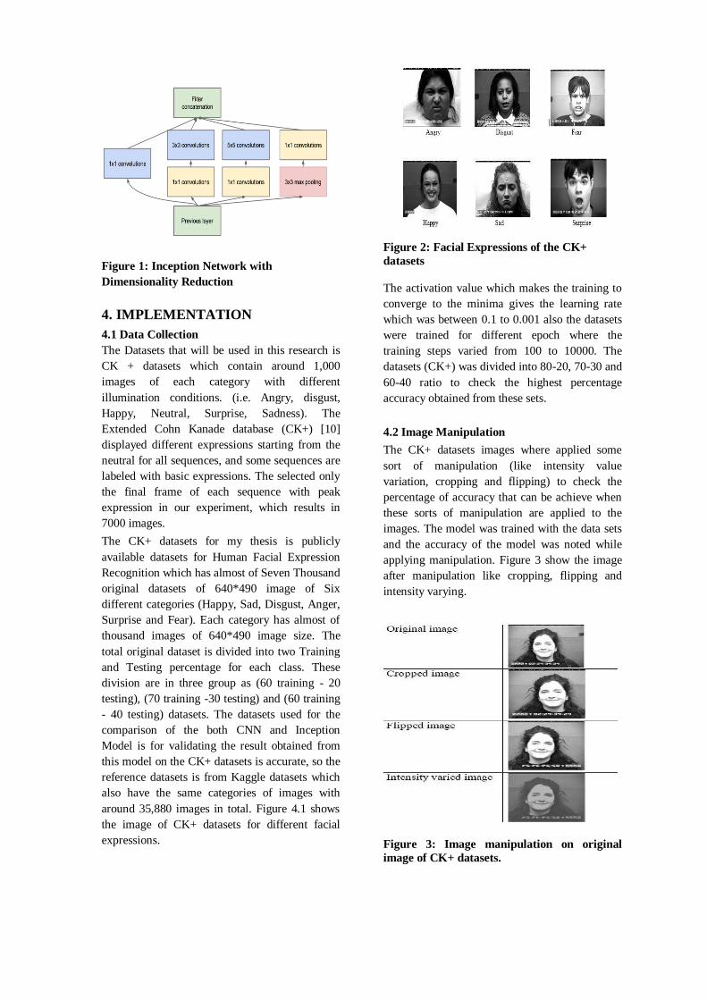
Figure 1: Inception Network with
Dimensionality Reduction
4. IMPLEMENTATION
4.1 Data Collection
The Datasets that will be used in this research is
CK + datasets which contain around 1,000
images of each category with different
illumination conditions. (i.e. Angry, disgust,
Happy, Neutral, Surprise, Sadness). The
Extended Cohn Kanade database (CK+) [10]
displayed different expressions starting from the
neutral for all sequences, and some sequences are
labeled with basic expressions. The selected only
the final frame of each sequence with peak
expression in our experiment, which results in
7000 images.
The CK+ datasets for my thesis is publicly
available datasets for Human Facial Expression
Recognition which has almost of Seven Thousand
original datasets of 640*490 image of Six
different categories (Happy, Sad, Disgust, Anger,
Surprise and Fear). Each category has almost of
thousand images of 640*490 image size. The
total original dataset is divided into two Training
and Testing percentage for each class. These
division are in three group as (60 training - 20
testing), (70 training -30 testing) and (60 training
- 40 testing) datasets. The datasets used for the
comparison of the both CNN and Inception
Model is for validating the result obtained from
this model on the CK+ datasets is accurate, so the
reference datasets is from Kaggle datasets which
also have the same categories of images with
around 35,880 images in total. Figure 4.1 shows
the image of CK+ datasets for different facial
expressions.
Figure 2: Facial Expressions of the CK+
datasets
The activation value which makes the training to
converge to the minima gives the learning rate
which was between 0.1 to 0.001 also the datasets
were trained for different epoch where the
training steps varied from 100 to 10000. The
datasets (CK+) was divided into 80-20, 70-30 and
60-40 ratio to check the highest percentage
accuracy obtained from these sets.
4.2 Image Manipulation
The CK+ datasets images where applied some
sort of manipulation (like intensity value
variation, cropping and flipping) to check the
percentage of accuracy that can be achieve when
these sorts of manipulation are applied to the
images. The model was trained with the data sets
and the accuracy of the model was noted while
applying manipulation. Figure 3 show the image
after manipulation like cropping, flipping and
intensity varying.
Figure 3: Image manipulation on original
image of CK+ datasets.
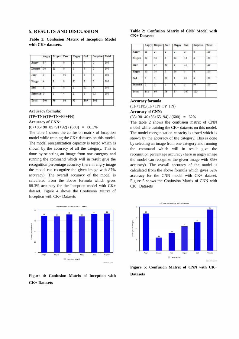
5. RESULTS AND DISCUSSION
Table 1: Confusion Matrix of Inception Model
with CK+ datasets.
Accuracy formula:
(TP+TN)/(TP+TN+FP+FN)
Accuracy of CNN:
(87+85+90+85+91+92) / (600) = 88.3%
The table 1 shows the confusion matrix of Inception
model while training the CK+ datasets on this model.
The model reorganization capacity is tested which is
shown by the accuracy of all the category. This is
done by selecting an image from one category and
running the command which will in result give the
recognition percentage accuracy (here in angry image
the model can recognize the given image with 87%
accuracy). The overall accuracy of the model is
calculated from the above formula which gives
88.3% accuracy for the Inception model with CK+
dataset. Figure 4 shows the Confusion Matrix of
Inception with CK+ Datasets
Figure 4: Confusion Matrix of Inception with
CK+ Datasets
Table 2: Confusion Matrix of CNN Model with
CK+ Datasets
Accuracy formula:
(TP+TN)/(TP+TN+FP+FN)
Accuracy of CNN:
(85+30+40+56+65+94) / (600) = 62%
The table 2 shows the confusion matrix of CNN
model while training the CK+ datasets on this model.
The model reorganization capacity is tested which is
shown by the accuracy of the category. This is done
by selecting an image from one category and running
the command which will in result give the
recognition percentage accuracy (here in angry image
the model can recognize the given image with 85%
accuracy). The overall accuracy of the model is
calculated from the above formula which gives 62%
accuracy for the CNN model with CK+ dataset.
Figure 5 shows the Confusion Matrix of CNN with
CK+ Datasets
Figure 5: Confusion Matrix of CNN with CK+
Datasets

Figure 6: Comparison of the accuracy obtained on
the both the model on CK+ datasets.
The confusion matrix for the CNN with Kaggle
dataset gives the accuracy of the model which is 70%
which is shown from [1] the confusion matrix for the
inception network with Kaggle dataset gives
accuracy as 82%. Similarly, for CK+ dataset the
inception network with 88.3% accuracy and the CNN
with 62% accuracy respectively. The low accuracy
of the CNN is due to its use of single filter in network
whereas inception network uses 1*1, 3*3, 5*5, 7*7
fitters together for feature extraction. The image of
CK+ and Kaggle dataset were applied some
distortion in the original images and with these
distorted images the network was trained, and the
accuracy were obtained which shows that the
inception network over all behaved to be good than
CNN as shown in figure 6.
6.CONCLUSION AND FUTURE WORK
The training accuracy for Inception Network was
88.3% with CK+ and 62% with Kaggle dataset.
Similarly training accuracy for CNN was 82% with
CK+ and 70% Kaggle dataset. The CK+ dataset was
applied some distortion to check the accuracy and
this was done on both the Inception network and
CNN network. The higher accuracy seen in Inception
model is as it uses the all the three convolutions i.e.
1*1 CONV, 3*3 CONV and 5*5 CONV together
which give the better result and also extract the lower
to higher features of the training image. This research
concludes that Inception Network has better
recognition capacity than that of CNN for images
with and without distortion in both the datasets.
Training the Inception Network took almost 5-6
hours with the 10000 training steps which was less as
compared to CNN which took around 8-9 hours.
Also, for manipulated image the training time
increased drastically which took more than a day for
inception network and 2 plus day for CNN. This can
be overcome by using GPU instead of CPU
processor. Also, the algorithm used can be further
enhanced which would make the computation faster
and increase accuracy.
7. REFERENCES
[1] Jinwoo Jeon, Jun Cheol Park, Young Joo Jo, "A
Real-time Facial Expression Recognizer using Deep
Neural Network", The 10th International Conference,
January 2016
[2]Alex Krizhevsky, Ilya Sutskever, Geoffrey E.
Hinton, "Image Net classification with deep
convolutional neural networks", The 25th
International Conference on Neural Information
Processing Systems ,Volume 1, December 03 - 06,
2012
[3]Christian Szegedy, Wei Liu, Yangqing Jia, Pierre
Sermanet, Scott Reed, Dragomir Anguelov, Dumitru
Erhan, Vincent Vanhoucke, Andrew Rabinovich;
"Going Deeper with Convolutions", Computer Vision
and Pattern Recognition (CVPR), IEEE International
Conference,7-12 June 2015
[4]Gerard Pons, David Masip," Supervised
Committee of Convolutional Neural Networks in
Automated Facial Expression Analysis", Transactions
on Affective Computing, IEEE International
Conference, September 201
[5] Junnan Li, Edmund Y. Lam, "Facial Expression
Recognition Using Deep Neural Network", Imaging
Systems and Techniques (IST), IEEE International
Conference 16-18 Sept. 2015
[6] Behzad Hasani, Mohammad H. Mahoor, " Facial
Expression Recognition Using Enhanced Deep 3D
Convolutional Neural Networks", Conference on
Computer Vision and Pattern Recognition
Workshops (CVPRW), 2017 IEEE ,Submitted on 22
May 2017
[7] Aysegul Ucar, "Deep Convolutional Neural
Networks for Facial Expression Recognition",
Innovations in Intelligent Systems and Applications
(INISTA), IEEE International Conference 08 August
2017
[8] Nitish Srivastava, Geoffrey E. Hinton, Alex
Krizhevsky, Ilya Sutskever, Ruslan Salakhut dinov,
"Dropout: a simple way to prevent neural networks
from over fitting", Journal of Machine Learning
Research, 2014

[9]Ariel Ruiz-Garcia, Mark Elshaw, Abdulrahman
Altahhan, Vasile Palade, "Stacked Deep
Convolutional Auto-Encoders for Emotion
Recognition from Facial Expressions, Neural
Networks (IJCNN) International Joint Conference on
03 July 2017

Fault Locating in Transmission Line Using Discrete Wavelet
Transform, Neural Network and Genetic Algorithm Ishir Babu Sharma, Shashidhar Ram Joshi
Department of Computer Engineering, Nepal College of Information Technology
9841883569, [email protected]
Abstract: This research compares three different
algorithms which can be used for locating faults in power
transmission lines where a neural network has been
trained using genetic algorithm with the combination of
two different types of fitness functions. The required
discrete fault current samples used for training the neural
network was acquired by the formula of three phase to
ground fault current. To extract the information of
different frequency bands of fault current discrete wavelet
transform has been used and to reduce the number of
inputs to the neural network, the energy of the
decomposition coefficients has been applied to the input
layers of the neural network.
Keywords: Discrete Wavelet Transform, Neural Network,
Genetic Algorithm, Power System Faults.
I. INTRODUCTION
Overhead transmission lines are parts of the electric power system where fault probabilities are generally higher than that
of other system components. Ground faults have been
considered as one of the main problems in power systems and
account for more than 80% of all faults. These faults give rise
to serious damage on power system equipments. A ground
fault which occurs on transmission lines not only effects the
equipments but also the power quality.
Therefore, it is very important to have a fast and reliable
method that can detect and locate faults on transmission lines in order to reduce the time needed to resume the service to
consumers and increase the reliability of the system.
Several methods have been proposed for locating fault in power transmission line. Silva, Lima and Souza [1] locate the
fault using the concept of complex domain neural network.
The fault current signal was transformed using Discrete
Fourier Transform (for the first case) and Stationary Wavelet
Transform (for the second case) and the neural network was
trained using complex domain back propagation algorithm
using complex domain hyperbolic tangent as an activation
function. Ekici, Yildirim and Poyraz [2] trained the neural
network using back propagation algorithm, where activation
function used were hyperbolic tangent sigmoid for first and
second layers and linear for the third layer. The input to the
neural network was energy and entropy of the Wavelet Packet
Coefficients of the fault current. Bhowmik, Purkait and
Bhattacharya [3] trained the neural network using back
propagation algorithm, where hyperbolic tangent sigmoid
function was used to activate the input nodes and linear
function was used to activate hidden and output nodes. The fault current signal was transformed using Discrete Wavelet
Transform. Mahanty and Gupta [4] trained the neural network
used to locate fault in transmission line that involves radial
basis function. Naggar [5] used the genetic algorithm to
optimize the fitness function (inverse of sum of square of
errors for the first case and inverse of sum of absolute value of
errors for the second case), where the errors involve the
difference between actual value of currents and outputs of
information vector (that depends on the distance of fault from
sending end) at discrete instants of time. Tawfik and Morcos
[6] used the Prony method to analyze the fault current signal
while training the neural network.
This research mainly aims to compare three different
algorithms which can be used for locating faults in power transmission lines built using discrete wavelet transform (to
decompose discrete values of fault current into different
frequency components), neural network (to learn the relation
between faulty distance and the energy of different frequency
components of the fault current) and genetic algorithm (to
train the neural network).
1.1 Artificial Neural Network An artificial neural network is made up of simple processing units
called neurons, which has a capacity for storing experimental
knowledge and making it available for use. It resembles the brain
in two respects:
a) Knowledge is acquired by the network from its environment
through a learning process.
b) Interneuron connection strengths, known as synaptic weights,
are used to store the acquired knowledge [10].
The design of neural networks proceeds as follows:
a) First an appropriate architecture is selected for the neural
network. The training data is used to train the neural
network by adjusting its synaptic weights.
b) Second the recognition performance of the trained
network is tested with data not seen before [10].

1.2 Genetic Algorithm
Genetic Algorithms are based on theory of natural selection
and work on generating a set of random solutions and make
them compete in an arena where only the fittest survive. Each
solution in the set is equivalent to a chromosome. A set of
chromosomes forms a population. The algorithm then uses
three basic operators: selection, crossover and mutation, together with a fitness function to evolve a new
population.[13].
1.3 Hybrid Systems
Here, the genetic algorithm is used to evolve the weights of
the neural network rather than using back propagation or some
other technique for training connection weights.
The chromosome in this case could be an ordered chain of
weights. Each neuron comprises the weights of the arcs that
connect the neuron of a layer to those of its previous layer.
Here the reciprocal of the sum of the square of errors
(
) or reciprocal of the sum of absolute value of
errors (
) reported after training the network for a
predetermined number of epochs could depict the fitness of a
set of weights.
Crossover cans be effected by swapping the genes. Mutation
can be effected by randomly adding or subtracting a small
value between 0 and 1 from weights that comprise a randomly
selected gene [13].
1.4 Discrete Wavelet Transform
The discrete wavelet transform (DWT) is a linear
transformation that operates on a data vector whose length is an integer power of two, transforming it into a numerically
different vector of the same length. It is a tool that separates
data into different frequency components, and then studies
each component with resolution matched to its scale. DWT is
computed with a cascading of filters followed by a factor 2
down sampling.
Figure.1: Block diagram of the discrete wavelet transform (h[n] and g[n]
denotes high and low-pass filters respectively, ↓ 2 denotes down sampling)
Outputs of these filters are given by the following equations:
(1)
(2)
Element aj is used for the next step of the transform and
element dj, called wavelet coefficient, determines the output
of the transform. g[n] and h[n] are coefficients of low and
high-pas filters respectively. For example, h[n] = {-1/2, -3/2,
3/2, 1/2}, g[n] = {1/8, 3/8, 3/8, 1/8} also called Daubechies
4/4 wavelet[12].
II. METHODOLOGY
The system in which the algorithm is applied is shown in
figure.2. It consists of a generator feeding a load center
through two transformers and a short transmission line. The
transmission line is 50 miles long and the line capacitance is
neglected. The fault is assumed to occur at different lengths from the sending end. Neglecting resistance, the symmetrical
short circuit current that flow in the transmission line can be
written as:
where,
E = sending end voltage
ω = angular frequency
Ǿ = voltage phase angle
Td1 = transient short circuit time constant
Td2 = sub transient short circuit time constant
Xd = xd + xt + xtl*L
Xd1 = xd1 + xt + xtl*L
Xd2 = xd2 + xt + xtl*L
xd = steady state reactance of generator
xd1 = transient reactance of generator
xd2 = sub transient reactance of generator
xt = transformer reactance
xtl = transmission line reactance
L = length of transmission line/mile at which the fault occurs[5]
Figure.2: A generator feeding a load center through two transformers and a
short transmission line
The block diagram of the method of development of programs
is shown in figure.3. At first equation 3 was used to generate
the fault current samples at different instants of time.
The discrete wavelet transform of the fault current samples
was generated using Daubechies 4/4 as a mother wavelet.
Since the lower frequency component of fault current contains
less information about the fault so the approximation
G
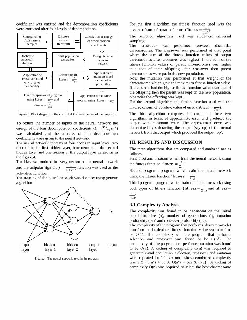
coefficient was omitted and the decomposition coefficients
were extracted after four levels of decomposition.
Figure.3: Block diagram of the method of the development of the programs
To reduce the number of inputs to the neural network the
energy of the four decomposition coefficients (
)
was calculated and the energies of four decomposition
coefficients were given to the neural network.
The neural network consists of four nodes in input layer, two
neurons in the first hidden layer, four neurons in the second
hidden layer and one neuron in the output layer as shown in
the figure.4.
The bias was omitted in every neuron of the neural network
and the unipolar sigmoid
function was used as the
activation function.
The training of the neural network was done by using genetic
algorithm.
Input hidden hidden output output
layer layer 1 layer 2 layer
Figure.4: The neural network used in the program
For the first algorithm the fitness function used was the
inverse of sum of square of errors (
).
The selection algorithm used was stochastic universal
sampling.
The crossover was performed between dissimilar
chromosomes. The crossover was performed at that point
where the sum of the fitness function values of output
chromosomes after crossover was highest. If the sum of the
fitness function values of parent chromosomes was higher
than that of their offspring after crossover then parent
chromosomes were put in the new population.
Now the mutation was performed at that weight of the
chromosome which gave the maximum fitness function value.
If the parent had the higher fitness function value than that of
the offspring then the parent was kept on the new population,
otherwise the offspring was kept.
For the second algorithm the fitness function used was the
inverse of sum of absolute value of error (
).
The third algorithm compares the output of these two
algorithms in terms of approximate error and produces the output with minimum error. The approximate error was
determined by subtracting the output (say op) of the neural
network from that output which produced the output ‘op’.
III. RESULTS AND DISCUSSION
The three algorithms that are compared and analyzed are as
follows:
First program: program which train the neural network using
the fitness function '
'
Second program: program which train the neural network
using the fitness function '
'
Third program: program which train the neural network using
both types of fitness function (
and
)
3.1 Complexity Analysis
The complexity was found to be dependent on the initial
population size (n), number of generations (i), mutation
probability (pm) and crossover probability (pc).
The complexity of the program that performs discrete wavelet
transform and calculates fitness function value was found to
be O(1). The complexity of the program that performs
selection and crossover was found to be O(n2). The
complexity of the program that performs mutation was found
to be O(n). A coding of complexity O(n) was required to
generate initial population. Selection, crossover and mutation
were repeated for ‘i’ iterations whose combined complexity was i X (O(n2) + pc X O(n2) + pm X O(n)). A coding of
complexity O(n) was required to select the best chromosome
Stochastic
universal
selection
Discrete
wavelet
transform
Calculation of energy
of decomposition
coefficients
Generation of
fault current
samples
Initial population generation
Energy input to
the neural network
Application of
crossover based
on crossover
probability
Calculation of
Application of
mutation based
on mutation
probability
Application of the same
program using
Error comparison of program
using
and
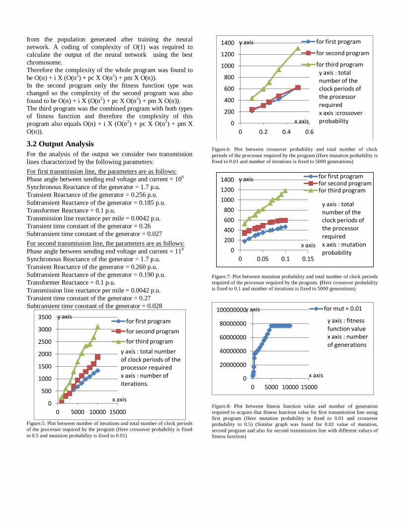
from the population generated after training the neural
network. A coding of complexity of O(1) was required to
calculate the output of the neural network using the best
chromosome.
Therefore the complexity of the whole program was found to
be O(n) + i X (O(n2) + pc X O(n2) + pm X O(n)).
In the second program only the fitness function type was
changed so the complexity of the second program was also
found to be O(n) + i X (O(n2) + pc X O(n2) + pm X O(n)).
The third program was the combined program with both types
of fitness function and therefore the complexity of this
program also equals O(n) + i X (O(n2) + pc X O(n2) + pm X
O(n)).
3.2 Output Analysis
For the analysis of the output we consider two transmission
lines characterized by the following parameters:
For first transmission line, the parameters are as follows:
Phase angle between sending end voltage and current = 100
Synchronous Reactance of the generator = 1.7 p.u.
Transient Reactance of the generator = 0.256 p.u.
Subtransient Reactance of the generator = 0.185 p.u.
Transformer Reactance = 0.1 p.u.
Transmission line reactance per mile = 0.0042 p.u.
Transient time constant of the generator = 0.26
Subtransient time constant of the generator = 0.027
For second transmission line, the parameters are as follows:
Phase angle between sending end voltage and current = 110
Synchronous Reactance of the generator = 1.7 p.u.
Transient Reactance of the generator = 0.260 p.u.
Subtransient Reactance of the generator = 0.190 p.u.
Transformer Reactance = 0.1 p.u.
Transmission line reactance per mile = 0.0042 p.u.
Transient time constant of the generator = 0.27
Subtransient time constant of the generator = 0.028
Figure.5: Plot between number of iterations and total number of clock periods
of the processor required by the program (Here crossover probability is fixed
to 0.5 and mutation probability is fixed to 0.01)
Figure.6: Plot between crossover probability and total number of clock
periods of the processor required by the program (Here mutation probability is
fixed to 0.01 and number of iterations is fixed to 5000 generations)
Figure.7: Plot between mutation probability and total number of clock periods
required of the processor required by the program. (Here crossover probability
is fixed to 0.1 and number of iterations is fixed to 5000 generations)
Figure.8: Plot between fitness function value and number of generation
required to acquire that fitness function value for first transmission line using
first program (Here mutation probability is fixed to 0.01 and crossover
probability to 0.5) (Similar graph was found for 0.02 value of mutation,
second program and also for second transmission line with different values of fitness function)
0
500
1000
1500
2000
2500
3000
3500
0 5000 10000 15000
for first program
for second program
for third program
y axis : total number of clock periods of the processor required x axis : number of iterations.
x axis
y axis
0
200
400
600
800
1000
1200
1400
0 0.2 0.4 0.6
for first program
for second program
for third program y axis : total number of the clock periods of the processor required x axis :crossover probability x axis
y axis
0
200
400
600
800
1000
1200
1400
0 0.05 0.1 0.15
for first program for second program for third program
y axis : total number of the clock periods of the processor required x axis : mutation probability
x axis
y axis
0
20000000
40000000
60000000
80000000
100000000
0 5000 10000 15000
for mut = 0.01
y axis : fitness function value x axis : number of generations
x axis
y axis
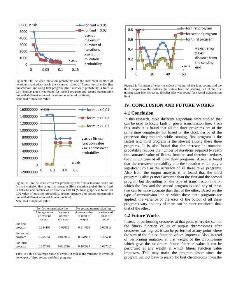
Figure.9: Plot between mutation probability and the maximum number of
iterations required to reach the saturated value of fitness function for first
transmission line using first program (Here crossover probability is fixed to
0.5) (Similar graph was found for second program and second transmission
line with different values of maximum number of iterations)
Note: mut = mutation value
Figure.10: Plot between crossover probability and fitness function value for
first transmission line using first program (Here mutation probability is fixed
to 0.06667 and number of iterations to 10000) (Similar graph was found for
0.01 value of mutation probability, second program and second transmission
line with different values of fitness function)
Note: mut = mutation value
For first transmission line For second transmission line
Average value
of error of
output
Variance
of error
of output
Average value
of error of
output
Variance of
error of
output
For first
program 0.334168 0.02852 0.214826 0.033811
For second
program 0.205851 0.041863 0.244982 0.07468
For third
program 0.157681 0.021726 0.188923 0.037315
Table.1: Table of average value of errors (in miles) and variance of errors of
the output of first, second and third programs.
Figure.11: Variation of error (in miles) of output of the first, second and the
third program as the distance (in miles) from the sending end of the first
transmission line increases. (Similar plot was found for second transmission
line)
IV. CONCLUSION AND FUTURE WORKS
4.1 Conclusion
In this research, three different algorithms were studied that can be used to locate fault in power transmission line. From
this study it is found that all the three programs are of the
same time complexity but based on the clock period of the
processor they required while running, first program is the
fastest and third program is the slowest among these three
programs. It is also found that the increase in mutation
probability reduces the number of iterations required to reach
the saturated value of fitness function and therefore reduces
the running time of all these three programs. Also it is found
that the crossover probability and the mutation value play a
significant role in the accuracy of all these three programs. Also from the output analysis it is found that the third
program is always more accurate than the first and the second
program but depending on the type of transmission line on
which the first and the second program is used any of these
two can be more accurate than that of the other. Based on the
type of transmission line on which these three programs are
applied, the variance of the error of the output of all these
programs vary and any of them can be more consistent than
that of the other.
4.2 Future Works
Instead of performing crossover at that point where the sum of
the fitness function values of output chromosomes after
crossover was highest it can be performed at any point where the sum of the fitness function values improves. Also, instead
of performing mutation at that weight of the chromosome
which gave the maximum fitness function value it can be
performed at any weight at which fitness function value
improves. This may make the program faster since the
program will not have to search for best chromosome from the
0
1000
2000
3000
4000
5000
6000
0 0.05 0.1 0.15
for mut = 0.01
for mut = 0.02
y axis : maximum number of iterations x axis : mutation probability
x axis
y axis
-20000000
0
20000000
40000000
60000000
80000000
100000000
120000000
140000000
160000000
0 0.2 0.4 0.6
for mut = 0.01
for mut = 0.02
for mut = 0.03
y axis : fitness function value x axis : crossover probability
x axis
y axis
0
0.2
0.4
0.6
0.8
0 20 40 60
for first program
for second program
for third program
y axis : error x axis : distance from the sending end
x axis
y axis

whole population during crossover and mutation. The
accuracy may be improved by changing the neural network
configuration to different forms and increasing the population
size. Also, variance of the error of the output can also be
added to the fitness function with suitable weight that may
lead to reduction in the variance of error.
ACKNOWLEDGEMENT
We would like to express our deepest appreciation to all those
who provided us the possibility to complete this report. We would also like to thank Assoc. Professor Mr. Saroj Shakya,
program coordinator of Master in Computer Engineering,
Nepal College of Information Technology for providing great
learning environment throughout this work.
REFERENCES
[1] Alexandre P. Alves da Silva, Antonio C.S. Lima, Suzana
M. Souza “Fault location on transmission lines using
complex domain neural networks” International Journal
of Electrical Power and Energy Systems (Volume: 43,
Issue: 1), December 2012, Pages 720-727
[2] Sami Ekici, Selcuk Yildirim, Mustafa Poyraz “Energy
and Entropy based feature extraction for locating fault on
transmission lines by using neural network and wavelet
packet decomposition” Experts systems and applications (Volume: 34, Issue: 4), May 2008, Pages 2937-2944
[3] P.S. Bhowmik, P. Purkait, K. Bhattacharya “A Novel
Wavelet Assisted Neural Network for Transmission Line
Fault Analysis” India Conference, 2008.INDICON 2008,
Annual IEEE (Volume: 1), 11-13 Dec 2008, Pages 223-
228
[4] 5.R.N. Mahanty, P.B. Dutta Gupta “Application of RBF
neural network to fault classification and location in
transmission lines” IEEE Proceedings – Generation,
Transmission and Distribution (Volume151, Issue 2),
March 2004 Pages 201-212
[5] K.M.EL-Naggar “A Genetic Based Fault Location
Algorithm for Transmission Lines” ieeexplore.ieee.org
Electricity Distribution, 200, Coll. of Technical School, Kuwait January 2001
[6] M. M. Tawfik and M. M. Morcos “ANN-Based
Techniques for Estimating Fault Location on
Transmission Lines Using Prony Method” IEEE
Tranctions on Power Delivery (Volume 16, No. 2) April
2001
[7] Damir Novosel, Bernhard Bachmann, David Hart, Yi Hu,
Murari Mohan Saha “Algorithms for Locating Faults on
Transmission Lines using Neural Network and
Deterministic Methods” IEEE Transactions on Power
Delivery (Volume 11,No. 4), October 1996
[8] Christopher M. Taylor “Selecting Neural Network Topologies: A Hybrid Approach Combining Genetic
Algorithms and Neural Network” www.ittc.ku.edu
Southwest Missouri State University, 1997
[9] Tania Pencheva, Krassimir Atanassov, Anthony
Shannon, "Modeling of Stochastic Universal Sampling
Selection operator in Genetic Algorithm Using
Generalized Nets" Tenth Int. Workshop on Generalized
Nets, 5 December 2009
[10] Simon Haykin “Neural Network A Comprehensive
Foundation” Second Edition
[11] B.R. Gupta “Power System Analysis And Design” Fifth Edition
[12] Sanjit K. Mitra “Digital Signal Processing” Fourth
Edition
[13] Elaine Ritch, Kevin Knight, Shivashankar B Nair
"Artificial Intelligence" Third Edition
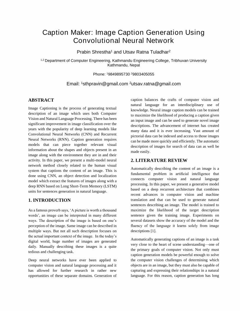
Caption Maker: Image Caption Generation Using Convolutional Neural Network
Prabin Shrestha1 and Utsav Ratna Tuladhar2
1,2 Department of Computer Engineering, Kathmandu Engineering College, Tribhuvan University
Kathmandu, Nepal
Phone: 19849895730 29803405055
Email: [email protected] [email protected]
ABSTRACT
Image Captioning is the process of generating textual
description of an image which uses both Computer
Vision and Natural Language Processing. There has been
significant improvement in image classification over the
years with the popularity of deep learning models like
Convolutional Neural Networks (CNN) and Recurrent
Neural Networks (RNN). Caption generation requires
models that can piece together relevant visual
information about the shapes and objects present in an
image along with the environment they are in and their
activity. In this paper, we present a multi-model neural
network method closely related to the human visual
system that captions the content of an image. This is
done using CNN, an object detection and localization
model which extract the features of images along with a
deep RNN based on Long Short-Term Memory (LSTM)
units for sentences generation in natural language.
1. INTRODUCTION
As a famous proverb says, ‘A picture is worth a thousand
words’, an image can be interpreted in many different
ways. The description of the image is based on one’s
perception of the image. Same image can be described in
multiple ways. But not all such description focuses on
the actual important context of the image. In the today’s
digital world, huge number of images are generated
daily. Manually describing these images is a quite
tedious and challenging task.
Deep neural networks have ever been applied to
computer vision and natural language processing and it
has allowed for further research in rather new
opportunities of these separate domains. Generation of
caption balances the crafts of computer vision and
natural language for an interdisciplinary use of
knowledge. Neural image caption models can be trained
to maximize the likelihood of producing a caption given
an input image and can be used to generate novel image
descriptions. The advancement of internet has created
many data and it is ever increasing. Vast amount of
pictorial data can be indexed and access to those images
can be made more quickly and efficiently. The automatic
description of images for search of data can as well be
made easily.
2. LITERATURE REVIEW
Automatically describing the content of an image is a
fundamental problem in artificial intelligence that
connects computer vision and natural language
processing. In this paper, we present a generative model
based on a deep recurrent architecture that combines
recent advances in computer vision and machine
translation and that can be used to generate natural
sentences describing an image. The model is trained to
maximize the likelihood of the target description
sentence given the training image. Experiments on
several datasets show the accuracy of the model and the
fluency of the language it learns solely from image
descriptions [1].
Automatically generating captions of an image is a task
very close to the heart of scene understanding—one of
the primary goals of computer vision. Not only must
caption generation models be powerful enough to solve
the computer vision challenges of determining which
objects are in an image, but they must also be capable of
capturing and expressing their relationships in a natural
language. For this reason, caption generation has long
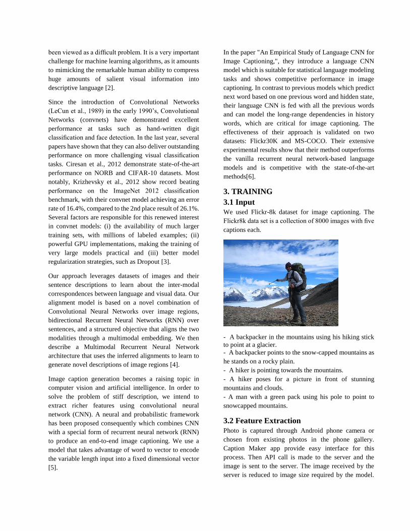
been viewed as a difficult problem. It is a very important
challenge for machine learning algorithms, as it amounts
to mimicking the remarkable human ability to compress
huge amounts of salient visual information into
descriptive language [2].
Since the introduction of Convolutional Networks
(LeCun et al., 1989) in the early 1990’s, Convolutional
Networks (convnets) have demonstrated excellent
performance at tasks such as hand-written digit
classification and face detection. In the last year, several
papers have shown that they can also deliver outstanding
performance on more challenging visual classification
tasks. Ciresan et al., 2012 demonstrate state-of-the-art
performance on NORB and CIFAR-10 datasets. Most
notably, Krizhevsky et al., 2012 show record beating
performance on the ImageNet 2012 classification
benchmark, with their convnet model achieving an error
rate of 16.4%, compared to the 2nd place result of 26.1%.
Several factors are responsible for this renewed interest
in convnet models: (i) the availability of much larger
training sets, with millions of labeled examples; (ii)
powerful GPU implementations, making the training of
very large models practical and (iii) better model
regularization strategies, such as Dropout [3].
Our approach leverages datasets of images and their
sentence descriptions to learn about the inter-modal
correspondences between language and visual data. Our
alignment model is based on a novel combination of
Convolutional Neural Networks over image regions,
bidirectional Recurrent Neural Networks (RNN) over
sentences, and a structured objective that aligns the two
modalities through a multimodal embedding. We then
describe a Multimodal Recurrent Neural Network
architecture that uses the inferred alignments to learn to
generate novel descriptions of image regions [4].
Image caption generation becomes a raising topic in
computer vision and artificial intelligence. In order to
solve the problem of stiff description, we intend to
extract richer features using convolutional neural
network (CNN). A neural and probabilistic framework
has been proposed consequently which combines CNN
with a special form of recurrent neural network (RNN)
to produce an end-to-end image captioning. We use a
model that takes advantage of word to vector to encode
the variable length input into a fixed dimensional vector
[5].
In the paper "An Empirical Study of Language CNN for
Image Captioning,", they introduce a language CNN
model which is suitable for statistical language modeling
tasks and shows competitive performance in image
captioning. In contrast to previous models which predict
next word based on one previous word and hidden state,
their language CNN is fed with all the previous words
and can model the long-range dependencies in history
words, which are critical for image captioning. The
effectiveness of their approach is validated on two
datasets: Flickr30K and MS-COCO. Their extensive
experimental results show that their method outperforms
the vanilla recurrent neural network-based language
models and is competitive with the state-of-the-art
methods[6].
3. TRAINING
3.1 Input
We used Flickr-8k dataset for image captioning. The
Flickr8k data set is a collection of 8000 images with five
captions each.
- A backpacker in the mountains using his hiking stick
to point at a glacier.
- A backpacker points to the snow-capped mountains as
he stands on a rocky plain.
- A hiker is pointing towards the mountains.
- A hiker poses for a picture in front of stunning
mountains and clouds.
- A man with a green pack using his pole to point to
snowcapped mountains.
3.2 Feature Extraction
Photo is captured through Android phone camera or
chosen from existing photos in the phone gallery.
Caption Maker app provide easy interface for this
process. Then API call is made to the server and the
image is sent to the server. The image received by the
server is reduced to image size required by the model.
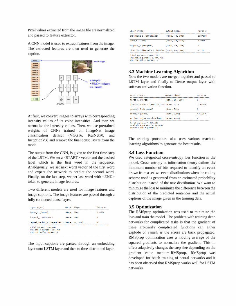
Pixel values extracted from the image file are normalized
and passed to feature extractor.
A CNN model is used to extract features from the image.
The extracted features are then used to generate the
caption.
At first, we convert images to arrays with corresponding
intensity values of its color intensities. And then we
normalize the intensity values. Then, we use pretrained
weights of CNNs trained on ImageNet image
classification dataset (VGG16, ResNet50, and
InceptionV3) and remove the final dense layers from the
mode
The output from the CNN, is given to the first time-step
of the LSTM. We set a <START> vector and the desired
label which is the first word in the sequence.
Analogously, we set next word vector of the first word
and expect the network to predict the second word.
Finally, on the last step, we set last word with <END>
token to generate image features.
Two different models are used for image features and
image captions. The image features are passed through a
fully connected dense layer.
The input captions are passed through an embedding
layer onto LSTM layer and then to time distributed layer.
3.3 Machine Learning Algorithm Now the two models are merged together and passed to
LSTM layer and finally to Dense output layer with
softmax activation function.
The training procedure also uses various machine
learning algorithms to generate the best results.
3.4 Loss Function We used categorical cross-entropy loss function in the
model. Cross-entropy in information theory defines the
minimum number of bits required to identify an event
drawn from a set two event distributions when the coding
scheme used is generated from an estimated probability
distribution instead of the true distribution. We want to
minimize the loss to minimize the difference between the
distribution of the predicted sentences and the actual
captions of the image given in the training data.
3.5 Optimization The RMSprop optimization was used to minimize the
loss and train the model. The problem with training deep
networks for complicated tasks is that the gradient of
these arbitrarily complicated functions can either
explode or vanish as the errors are back propagated.
RMSprop optimization uses a moving average of the
squared gradients to normalize the gradient. This in
effect adaptively changes the step size depending on the
gradient value medium-RMSprop. RMSprop was
developed for batch training of neural networks and it
has been observed that RMSprop works well for LSTM
networks.

4. PREDICTION
Test images are used to extract features from them using
the same feature extraction model. The captions for new
images are then generated using search algorithms –
normal max search and beam search.
4.1 Normal Max Search To perform inference, we first obtain image embedding
by passing the image through the CNN model and then
the dense layer. Then to generate captions using the
model, we first feed the LSTM cell with < start> as the
first input and image embedding as its initial states. The
LSTM produces a word and its hidden states, and we
keep feeding this word and hidden states again to the
LSTM cell until it outputs < end> or reaches the max
sentence length. At first <start> is feed into LSTM cell
as input and the word with max probability is selected.
Both are again feed to LSTM cell and next word with
max probability is chosen and so on until <end> is
selected or max sentence length is reached.
4.2 Beam Search In Beam Search, we take top k predictions, feed them
again in the model and then sort them using the
probabilities returned by the model. So, the list will
always contain the top k predictions. In the end, we take
the one with the highest probability and go through it till
we encounter <end> or reach the maximum caption
length. We used various beam sizes for our experiments.
5. EVALUATION METRICS
At first, two models for image feature and image
captions were created. The model for image features
Table 1: Results for initial model
consists of input layer which takes image features
extracted from imagenet model, a dropout layer and an
output dense layer. The model for image captions
consists of an embedding layer, a dropout layer and
LSTM layer. The output from two models were
concatenated and passed through two dense layers to
form a final model.
Initially, for image feature extraction we used the VGG-
16 model followed by InceptionV3 model and obtained
the results as shown in Table1.
New models for image features and image captions were
created to improve the loss. The model for image
features consists of input denser layer which takes image
features extracted from imagenet model and a repeat
vector layer. The model for image captions consists of
an embedding layer, a LSTM layer and a Time
Distributed LSTM layer. The output from two models
were concatenated and passed through a Bidirectional
LSTM layer and a dense layer to form the final model.
The output was obtained after using softmax activation
as shown in Table2.
Table 2: Results for final model
6. RESULTS
6.1 Comparison
Input captions as in the dataset:
- A backpacker in the mountains using his hiking stick
to point at a glacier.
- A backpacker points to the snow-capped mountains as
he stands on a rocky plain.
- A hiker is pointing towards the mountains.
- A hiker poses for a picture in front of stunning
mountains and clouds.
- A man with a green pack using his pole to point to
snowcapped mountains.
Model VGG-16 InceptionV3
Epoch 20 20
Loss 3.21 3.1
Validation
loss
3.8 3.6
BLEU
scores
BLEU-1: 0.502664
BLEU-2: 0.258071
BLEU-3: 0.173180
BLEU-4: 0.075685
BLEU-1: 0.515913
BLEU-2: 0.302460
BLEU-3: 0.222020
BLEU-4: 0.115490
New
model
VGG-16 InceptionV3
(without dropout)
InceptionV3
(with dropout)
Epoch 35 10 25
Batch
size
128 512 756
Loss 2.77 1.8 1.6
BLEU
scores
BLEU-1: 0.61403
BLEU-2: 0.40659
BLEU-3: 0.32191
BLEU-4: 0.20892
BLEU-1: 0.61403
BLEU-2: 0.40659
BLEU-3: 0.32191
BLEU-4: 0.20892
BLEU-1: 0.62931
BLEU-2: 0.46231
BLEU-3: 0.39317
BLEU-4: 0.26824

Generated caption:
A backpacker points to mountains and clouds.
This way, during training process, a caption is generated
from the input picture and its captions.
6.2 Outputs The following photos generated the following photos
from this model.
A boy does tricks on a
bicycle at a skate park.
A boy does tricks on a
bicycle at a skate park.
A man in blue pants
standing. A white building with
windows.
A man in a black jacket is riding a bike on a dirt
road.
A man in white shirt posing in front of a wall.
A man in white shirt standing behind a man in
white shirt

7. CONCLUSION
This research work uses Convolutional Neural Networks
and RNN based LSTM units to generate a caption from
an image. At the end, we were able to train a model with
a bleu score accuracy of 43% using InceptionV3 model
with dropouts. The loss of 1.6 was obtained with it. More
experiments on several datasets like Flickr30k and the
MS-COCO dataset could be done to generate a model
with even better accuracy.
ACKNOWLEDGEMENT
We would like to thank Dr. Basanta Joshi for
advising us for the publication of this research
paper.
REFERENCES
[1] O. T. A. B. S. a. E. D. Vinyals, "Show and Tell: A
Neural Image Caption Generator," arXiv, no.
1411.4555, Novemember 2014.
[2] L. K. C. C. S. Z. B. Xu, "Show,Attend and Tell :
Neural Image Caption Generation with Visual
Attention," arXiv, vol. 3, no. 1502.03044, 19 April
2016.
[3] F. D. Zeiler, "Visualizing and Understanding
Convolutional Networks," arXiv, no. 1311.2901,
23 Nov 2013.
[4] F.-F. L. Karpathy Andrej, "Deep Visual-Semantic
Alignments for Generating Image Descriptions,"
IEEE Transactions on Pattern Analysis and
Machine Intelligence, vol. 39, no. 4, pp. 664 - 676,
05 August 2016.
[5] S. Ding, Y. Xi and S. Qu, "Visual attention based
on long-short term memory model for image
caption generation," Control And Decision
Conference (CCDC), 2017.
[6] D. Y. \. Kim Dong-Jin, "An Empirical Study of
Language CNN for Image Captioning," 2017 IEEE
International Conference on Computer Vision
(ICCV), 25 December 2017.
Handwritten Devanagari Character Recognition using Capsule Network
Kumar LamichhaneMasters of Computer Engineering
Nepal College of Information TechnologyBalkumari, Lalitpur, Nepal
Abstract— This thesis proposes a Capsule Network (CapsNet)to classify the Handwritten Devanagari Characters. We takea brief look into the shortcomings of Convolutional NeuralNetwork (ConvNet). A CapsNet model is proposed to solvethe shortcomings of ConvNet and perform the test comparablyaccurately. The performance analysis of the network is done onMNIST digits and publicly available Devanagari HandwrittenCharacter dataset and also on geometrically transformed (ro-tated, scaled, sheared) test datasets. A ConvNet model is alsotested for the datasets and the performances of both the modelsare compared.
The handwritten devanagari characters are recognized bythe experimental CapsNet model with 99.69% accuracy andfor the same dataset accuracy of ConvNet is 98.96%.
Keywords: Computer Vision, Handwritten character recog-nition, Convolutional Neural Network(CNN, ConvNet), CapsuleNeural Network (CapsNet)
I. INTRODUCTION
Object recognition and Image classification has alwaysbeen the center of computer vision problems. The currentstate of art in image classification and object recognition isthe Convolutional Neural Networks(CNN). CNN has evenoutperformed human in object recognition and image classi-fication problems. But the CNN is said to be doomed because
1) CNN cannot handle spatial relations between objectparts
2) CNN needs to be trained for orientation and perspec-tive change
3) CNN is vulnerable to perturbation attacksThus, the shortcomings of CNN motivated Geoffrey Hintonto propose Capsules[1], which are the nested set of neurons.This research explores the generalization capability of Cap-sNet on geometrically transformed images.
II. RESEARCH OBJECTIVE
The objectives of this research are1) To recognize handwritten Devanagari characters using
Capsule Network2) To find and analyze the performance of Capsule Net-
work over geometrically transformed (rotate, scale,shear) images.
III. DATASETS
• Devanagari Handwritten Character Dataset
Introduces a new publicly available dataset, Devanagari
Fig. 1. Computational Graph of the experimental model as shown bytensorboard
Handwritten Character Dataset, of 92 thousand 28*28images of 46 Devanagari characters out of which 10 arenumerals and 36 are consonants.
• Modified National Institute of Standards and Technol-ogy (MNIST)MNIST is a popular and widely used machine learningdataset of handwritten digits consists of a training setof 60,000 examples, and a test set of 10,000 examples.
IV. PROPOSED MODEL
The tensorflow dataflow graph represents the computationin terms of the dependencies between individual opera-tions[10]. Fig. 1 shows the dataflow graph of the experimen-tal model as shown by the visualization library, tensorboard.
V. METHODOLOGY
Fig. 2 shows the steps carried out to complete this researchwork.
VI. EXPERIMENTS AND RESULTS
A CapsNet and a ConvNet were trained with MNIST andDevanagari Handwritten Character Dataset and tested withdifferent geometric transformations.
Fig. 2. Research Methodology
Fig. 3. Training Accuracy & Loss (20 epoch)
A. Training
The network was trained for 20epoch. Fig. 3. shows thegraph of training process and Table. 1. shows the trainingaccuracy on different epoch of training.
TABLE ITEST ACCURACY, VALIDATION ACCURACY AND LOSS FOR DIFFERENT
EPOCHS
01epoch 05epoch 10epoch 20epochtraining accuracy 0.9718 1.0 1.0 1.0validation accu-racy
0.9776 0.9866 0.9932 0.9977
loss 0.0754 0.0132 0.0187 0.0070
B. Testing
Both MNIST and Devanagari Handwritten Characterdatasets were tested on the CapsNet and ConvNet models.Table II, III, IV, V shows the results of tests on the trainedexperimental model on different datasets.
TABLE IICOMPARATIVE TEST ACCURACIES OF CAPSNET & CONVNET ON
MNIST & DEVANAGARI CHARACTERS
test dataset ConvNet CapsNetMNIST Devanagari MNIST Devanagari
original 0.9804 0.9830 0.9896 0.9969rotated(0-360) 0.4071 0.2973 0.431 0.3996scaled(0.5-1.1) 0.5593 0.2716 0.564 0.3287sheared(0-0.9) 0.1800 0.2376 0.223 0.3661
TABLE IIICOMPARATIVE TEST ACCURACIES OF THE EXPERIMENTAL CAPSNET &
CONVNET MODEL ON MNIST & DEVANAGARI CHARACTERS FOR
DIFFERENT ANGLES OF ROTATION
rotation angle ConvNet CapsNetMNIST Devanagari MNIST Devanagari
random(0-360) 0.4071 0.2973 0.431 0.39961-degree 0.9882 0.9883 0.9896 0.996310-degree 0.9756 0.9583 0.9826 0.993630-degree 0.8355 0.5989 0.8486 0.807645-degree 0.5097 0.3526 0.5136 0.445360-degree 0.195 0.2263 0.2486 0.230375-degree 0.067 0.1533 0.1695 0.1763
TABLE IVCOMPARATIVE TEST ACCURACY OF CAPSNET & CONVNET ON MNIST
& DEVANAGARI CHARACTERS FOR DIFFERENT SCALE FACTORS
scaled ConvNet CapsNetMNIST Devanagari MNIST Devanagari
random(0.5-1.1) 0.5593 0.2716 0.564 0.32871.11 0.8988 0.868 0.9053 0.96530.66 0.1445 0.1853 0.178 0.39960.5 0.0553 0.0286 0.085 0.0643
TABLE VCOMPARATIVE TEST ACCURACIES OF CAPSNET AND CONVNET MODEL
ON MNIST & DEVANAGARI CHARACTERS FOR DIFFERENT SHEAR
VALUES
shear value ConvNet CapsNetMNIST Devanagari MNIST Devanagari
random(0-0.9) 0.18 0.2376 0.223 0.36610.2 0.5338 0.6063 0.533 0.8710.5 0.0841 0.1113 0.10 0.2080.7 0.0831 0.0496 0.083 0.098
VII. CONCLUSION
Training accuracy of the experimental CapsNet model was100% after 20epoch of training which evaluated the originaldataset with 99.69% accuracy. For every test dataset we cansee that the evaluation accuracy of the CapsNet model isslightly better than that of the ConvNet model.Hence this research can conclude that CapsNet has slightlybetter generalization capability than that of ConvNet forgeometrically transformed images.
VIII. LIMITATIONS AND FUTURE WORKS
Training the CapsNet model for 1 epoch took almost45 minutes which is comparably very much than that ofConvNet. The training can be accelerated by using GPUs.

[3] describes a new architecture, Matrix Capsules with(Expectation Maximization)EM routing with different layersand EM Routing algorithm. The Routing by Agreementalgorithm can be replaced by the EM Routing algorithm andperformance could be analyzed. The work depicted on thisthesis can be a reference for the facial recognition, objectrecognition tasks as well.
REFERENCES
[1] Sabour, S., Frosst, N., & Hinton, G. (2017). Dynamic Routing BetweenCapsules.
[2] Balci, B., Saadati, D., Shiferaw D. (2016). Handwritten Text Recog-nition using Deep Learning.
[3] MATRIX CAPSULES WITH EM ROUTING , ICLR 2018 ConferenceBlind Submission, 2017
[4] Su, J., Vargas, D., & Kouichi, S. (2017). One pixel attack for foolingdeep neural networks.
[5] Acharya, S., Pant, A., & Gyawali, P. (2015). Deep learning basedlarge scale handwritten Devanagari character recognition. Software,Knowledge, Information Management and Applications (SKIMA),2015 9th International Conference on, 1-6.
[6] Max Pechyonkin (2018) Understanding Hintons Cap-sule Networks. Medium[online]. Available from:https://medium.com/@pechyonkin/part-iv-capsnet-architecture-6a64422f7dce [Accessed 1st March 2018]
[7] Jaiswal, A., AbdAlmageed, W., Wu, Y., & Natarajan, P. (2018).CapsuleGAN: Generative Adversarial Capsule Network.
[8] Qiao, K., Zhang, C., Wang, L., Yan, B., Chen, J., Zeng, L., & Tong, L.(2018). Accurate reconstruction of image stimuli from human fMRIbased on the decoding model with capsule network architecture.
[9] Engelin, Martin. (2018) CapsNet Comprehension of Objects in Dif-ferent Rotational Views.
[10] Faizan, Shaikh., (2018) Essentials of Deep Learning:Getting to know CapsuleNets[online]. Available from:https://www.analyticsvidhya.com/blog/2018/04/essentials-of-deep-learning-getting-to-know-capsulenets/ [Accessed 1st May 2018]
[11] Xi, E., Bing, S., & Jin, Y. (2017). Capsule Network Performance onComplex Data.
[12] Iesmantas, T., & Alzbutas, R. (2018). Convolutional capsule networkfor classification of breast cancer histology images.
[13] Kim, Y., Wang, P., Zhu, Y., & Mihaylova, L. (2018). A CapsuleNetwork for Traffic Speed Prediction in Complex Road Networks.
[14] Nguyen, Dai Quoc, Vu, Thanh, Nguyen, Tu Dinh, & Phung, Dinh.(2018). A Capsule Network-based Embedding Model for SearchPersonalization.
[15] Li, Yu., Qian, Meiyu., Liu, Pengfeng., Cai, Qian., Li, Xiaoying., Guo,Junwen., . . . Zhou, Ziwei. (2018). The recognition of rice images byUAV based on capsule network. Cluster Computing, 1-10.
[16] Huadong, Liao. (2018). Available from:https://github.com/naturomics/CapsNet-Tensorflow [Accessed Nov2017]
[17] Zhao, Wei., Ye, Jianbo., Yang, Min., Lei, Zeyang., Zhang, Suofei., &Zhao, Zhou. (2018). Investigating Capsule Networks with DynamicRouting for Text Classification.
[18] UCI Machine Learning Repository, Available from:https://archive.ics.uci.edu/ml/datasets/Devanagari+Handwritten+Character+Dataset[Accessed Nov 2017]
[19] Nair, Prem., Doshi, Rohan., Keselj, Stefan. (2018).Pushing the Limitsof Capsule Networks

Sentence Ranking and Answer Pinpointing inOnline Discussion Forums Utilising User-generated
Metrics and HighlightsSushant Gautam∗, Saloni Shikha †, Alina Devkota ‡ and Spandan Pyakurel§
Department of Electronics and Computer Engineering, Pulchowk CampusInstitute of Engineering, Tribhuwan Univeristy
Lalitpur, NepalEmail: ∗[email protected], †[email protected], ‡[email protected], §[email protected]
Abstract—One of the major challenges in searching on theinternet has been that search engines and online forums have notbeen able to extract and pinpoint exact answer to people’s querydespite information being available on the internet. Extractionof to-the-point answers from articles, posts and blogs tendto improve search accuracy. Sentence Ranking helps to rankanswers according to a score that represents positive remarkfor the relevance of sentence. User-generated metrics can beused to improve sentence ranking. Also, the text selected andsaved as highlights by users can be used to extract the mostimportant parts of the content. Answer pinpointing in simpleforums can be achieved by allowing users to highlight parts ofthe text, store it in a database and analyse such highlights usingsentence ranking engine followed by answer extraction to find thebest chunk of texts. It can prove to be a milestone in providingexact and relevant answers as per the searchers’ intent and canalso facilitate improvement of question answering in discussionforums.
Index Terms—sentence ranking, user-generated content, ques-tion answering, user-generated metric, user highlights, answerpinpointing, online discussion forum, engagement metric.
I. INTRODUCTION
Active research is being conducted in the field of questionanswering (QA) and information retrieval. Intelligent agentsand bots are already showing their presence in the globalmarket and are being smarter each day. The results, however,have shown that the progress in this field is yet too far fromfulfilling the expectations. The Internet has a massive amountof data but, diverse and unlabelled. That is why the searchengines and assistants, in spite of having access to a massiveamount of data, have not been able to give users the exactanswers to the questions they have been searching for. Also,to address users’ immediate information need, it is necessaryto have a good information retrieval system. This can be donethrough the creation of an ideal question-answer system.
In search engines, widely searched questions such as ”Whatis the height of the Everest?” are provided with exact answers.This, however, is not the case with other questions. Even whenthe answers to the questions searched for are available onthe internet, they are not pinpointed. Identifying the preciseanswer within a long text has thus been a challenge in onlinediscussion forums. Pinpointing the answer requires ranking
of the sentences which may possibly contain the answerand extracting it. Different techniques and algorithms aid theprocess and are in use. Recent researches have shown thatneural networks can be used to enhance question-answeringsystems thus providing users with better search experience.
II. BACKGROUND
Answer Sentence Ranking and Answer Extraction are thetwo major challenges in question-answering required for thepurpose.
A. Sentence Ranking
Answer sentence selection has always been a topic of inter-est to researchers in the field of question-answering systems.Answer sentence ranking involves assigning different answersto a question with a rank according to the relevance of theanswers. The one that is ranked higher is the one that is morelikely to have the answer contained in it (see Fig. 1).
A tag is a label attached to a post for purpose of identi-fication or categorisation that can be several words long andreflects key points of the post. Tags can be either automaticallygenerated from a passage or inserted by users themselves.Tags help to increase search efficiency by finding exact matchrather than conventional techniques where strings are searchedby matching sub-strings. Characteristics of tags often havea direct relationship with the users’ answers. Sometimeshierarchies of tags can be used by nesting related tags intoa collapsible list. Tags can also be helpful to answer sentenceranking.
Likewise, one of the most popular meta-data tags used insocial platforms, such as Instagram, Facebook, Pinterest andGoogle+ is the hashtag that allows users to apply dynamictagging for the purpose of the ease in the finding of postswith specific contents. Hashtags are focused more by viewersbut they also serve as links to search queries.
According to Dwivedi and Singh[1], possible approaches foranswer ranking are Linguistic Approach, Statistical Approachand Pattern Matching Approach.
1) Linguistic Approach for Answer Ranking: The linguisticapproach relies on the use of Artificial Intelligence
Fig. 1: QA based System Implementation Model
techniques integrating with Natural Language Process-ing techniques and knowledge base to form question-answering logic. Information organised in the formof production rules, logic, frames, templates, ontologyand semantic networks are utilised during analysis ofquestion-answer pair. Sometimes knowledge-based QAsystems rely on a rule-based mechanism to identifyquestion classification features.
2) Statistical Approach: This approach deals with a largeamount of data and their heterogeneity and is inde-pendent of a query language. Support vector machine(SVM) classifiers, Bayesian classifiers, Maximum en-tropy models are some techniques that have been usedfor question classification purpose. Pattern matchingapproach uses text patterns or templates to identifyanswers.
3) Pattern Matching Approach: This approach uses textpatterns or templates to identify answers. For example,the question, “When did world war II end?”, followsthe pattern “When did <event name> end?” and itsanswer pattern will be like “<event name> ended on<date/time>”. Systems can be made to learn suchtext patterns from text passages rather than employingcomplicated linguistic knowledge or tools to text forretrieving answers.
B. Answer Extraction
The answers to questions posted in forums may or maynot contain the exact answers to the questions in the thread.Answer extraction deals with extracting smaller parts (whichmay be in the form of words, phrases or sentences) from longposts for providing the readers with the precise answer to thequestion. Sentence ranking is followed by answer extractionwhere the answers are extracted. Sultan[2], in his paper, hasexplained the generic framework that is followed by most ofthe extraction algorithms. For any question, there are candidateanswer sentences from each of which chunks of texts are
identified. These chunks are, then, evaluated according tosome criterion. The criterion depends on the method used.The best chunk is then identified. After we have located thebest chunks from different sentences, equivalent chunks aregrouped together and the quality of each group is computed.Finally, a chunk is extracted from the best group supposed tobe the most precise answer to the given question.
C. Web 2.0 and Internet Revolution
The term ‘Web 2.0’ was invented by Darcy DiNucci in1999 and got popularised at the O’Reilly Media Web 2.0Conferences in late 2004[3]. Websites in Web 2.0 alloweduser interactions and collaborations in a virtual communityas creators of user-generated content. The idea behind Web2.0 was very distinct at that time before which the web onlyallowed visitors from viewing the static content without sig-nificant interactions. The idea of Web 2.0 can be decomposedinto three components: Rich Internet Application (RIA), Web-Oriented Architecture (WOA) and Social Web. Web 2.0 sitesincluded various features and techniques including search,extensions and signal which Andrew McAfee referred by theacronym SLATES[4].
Like all other things, internet sites have also undergone botha revolution and an evolution. As the global push towards on-line presence and information sharing continues, websites andforum platforms have also emerged and bloomed. Currently,we have access to a diverse range of contents than ever andthe trend continues. Only in 2016, around 96,000 petabytesof information was transferred which was double than that in2012[5]. On the other hand, there are already over a billionwebsites all over the internet full of information over diverserange[6].
III. RELATED WORKS
As the web and the virtual digital assistant technologies areenhancing, various works have been done on almost all majoraspects of answer extraction, sentence ranking and answerpinpointing.
A. Answer sentence selection
Echihabi and Marcu, 2003[7], have explained question-answering system as a pipeline of only two high level modules:An Information retrieval engine that obtains information sys-tem resources R relevant to an information that may containanswers to a given question Q1 and an answer identifiermodule which ranks each information resource for its rele-vancy with question Q1. For example, if a whole sentenceS from resource R is accepted as the most likely answer,cosine similarity between S and Q1 can be used to calculatethe likelihood of an answer. Researches have shown that suchword-overlap method is practically not a good enough metricfor answer selection. Enhanced Models of lexical semanticresources have improved the performance over systems whichfocuses only on syntactic analysis through dependency treematching [8].
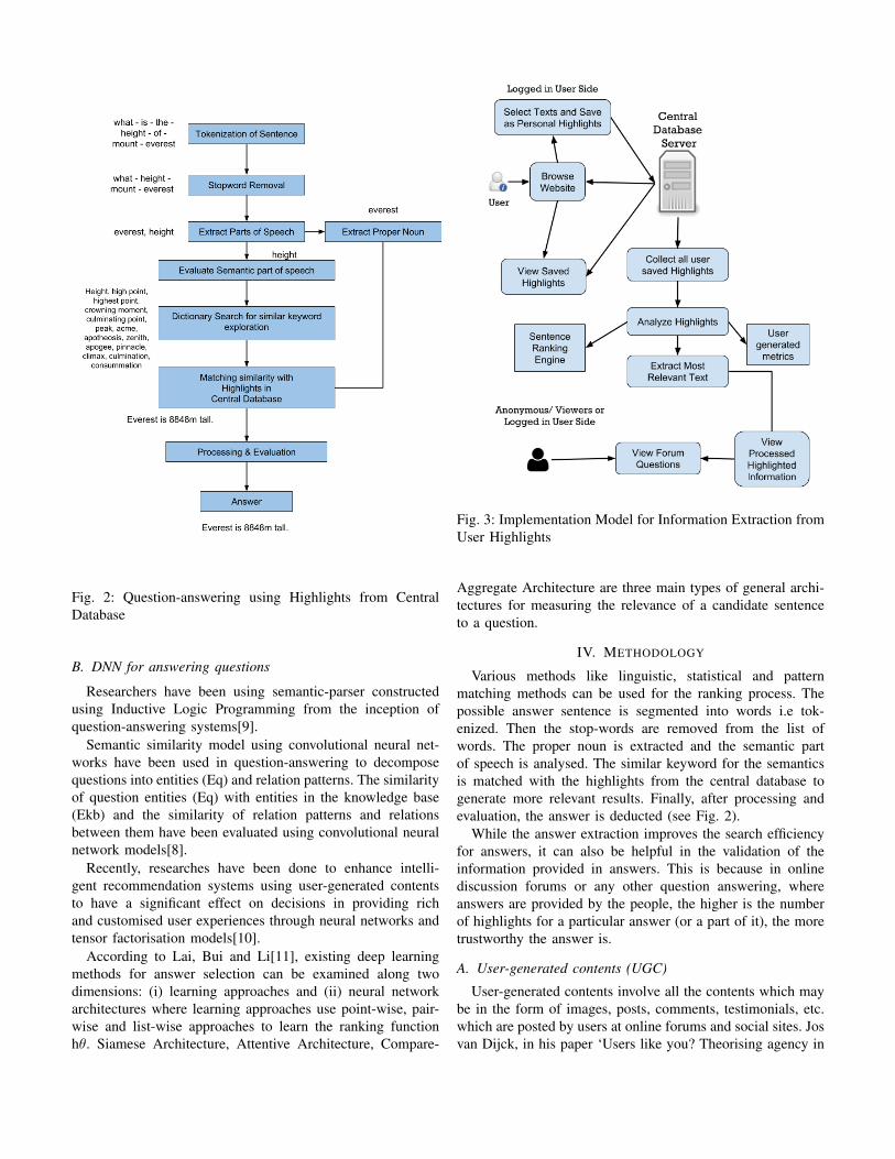
Fig. 2: Question-answering using Highlights from CentralDatabase
B. DNN for answering questions
Researchers have been using semantic-parser constructedusing Inductive Logic Programming from the inception ofquestion-answering systems[9].
Semantic similarity model using convolutional neural net-works have been used in question-answering to decomposequestions into entities (Eq) and relation patterns. The similarityof question entities (Eq) with entities in the knowledge base(Ekb) and the similarity of relation patterns and relationsbetween them have been evaluated using convolutional neuralnetwork models[8].
Recently, researches have been done to enhance intelli-gent recommendation systems using user-generated contentsto have a significant effect on decisions in providing richand customised user experiences through neural networks andtensor factorisation models[10].
According to Lai, Bui and Li[11], existing deep learningmethods for answer selection can be examined along twodimensions: (i) learning approaches and (ii) neural networkarchitectures where learning approaches use point-wise, pair-wise and list-wise approaches to learn the ranking functionhθ. Siamese Architecture, Attentive Architecture, Compare-
Fig. 3: Implementation Model for Information Extraction fromUser Highlights
Aggregate Architecture are three main types of general archi-tectures for measuring the relevance of a candidate sentenceto a question.
IV. METHODOLOGY
Various methods like linguistic, statistical and patternmatching methods can be used for the ranking process. Thepossible answer sentence is segmented into words i.e tok-enized. Then the stop-words are removed from the list ofwords. The proper noun is extracted and the semantic partof speech is analysed. The similar keyword for the semanticsis matched with the highlights from the central database togenerate more relevant results. Finally, after processing andevaluation, the answer is deducted (see Fig. 2).
While the answer extraction improves the search efficiencyfor answers, it can also be helpful in the validation of theinformation provided in answers. This is because in onlinediscussion forums or any other question answering, whereanswers are provided by the people, the higher is the numberof highlights for a particular answer (or a part of it), the moretrustworthy the answer is.
A. User-generated contents (UGC)
User-generated contents involve all the contents which maybe in the form of images, posts, comments, testimonials, etc.which are posted by users at online forums and social sites. Josvan Dijck, in his paper ‘Users like you? Theorising agency in
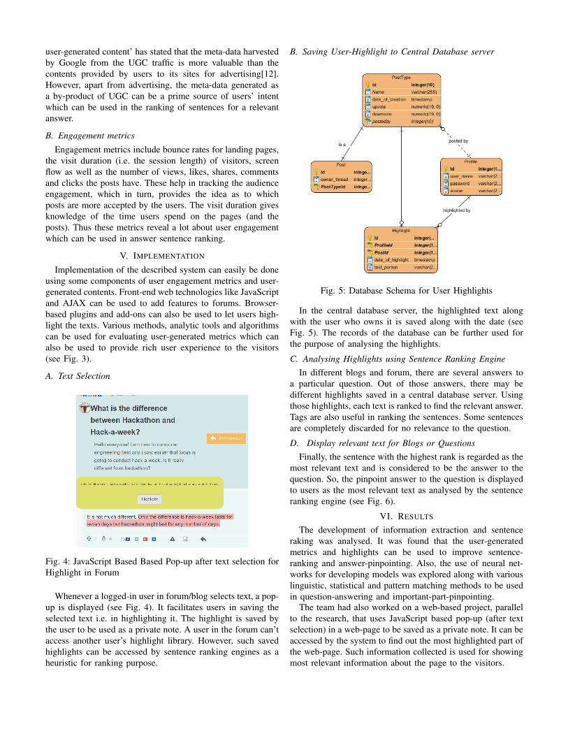
user-generated content’ has stated that the meta-data harvestedby Google from the UGC traffic is more valuable than thecontents provided by users to its sites for advertising[12].However, apart from advertising, the meta-data generated asa by-product of UGC can be a prime source of users’ intentwhich can be used in the ranking of sentences for a relevantanswer.
B. Engagement metrics
Engagement metrics include bounce rates for landing pages,the visit duration (i.e. the session length) of visitors, screenflow as well as the number of views, likes, shares, commentsand clicks the posts have. These help in tracking the audienceengagement, which in turn, provides the idea as to whichposts are more accepted by the users. The visit duration givesknowledge of the time users spend on the pages (and theposts). Thus these metrics reveal a lot about user engagementwhich can be used in answer sentence ranking.
V. IMPLEMENTATION
Implementation of the described system can easily be doneusing some components of user engagement metrics and user-generated contents. Front-end web technologies like JavaScriptand AJAX can be used to add features to forums. Browser-based plugins and add-ons can also be used to let users high-light the texts. Various methods, analytic tools and algorithmscan be used for evaluating user-generated metrics which canalso be used to provide rich user experience to the visitors(see Fig. 3).
A. Text Selection
Fig. 4: JavaScript Based Based Pop-up after text selection forHighlight in Forum
Whenever a logged-in user in forum/blog selects text, a pop-up is displayed (see Fig. 4). It facilitates users in saving theselected text i.e. in highlighting it. The highlight is saved bythe user to be used as a private note. A user in the forum can’taccess another user’s highlight library. However, such savedhighlights can be accessed by sentence ranking engines as aheuristic for ranking purpose.
B. Saving User-Highlight to Central Database server
Fig. 5: Database Schema for User Highlights
In the central database server, the highlighted text alongwith the user who owns it is saved along with the date (seeFig. 5). The records of the database can be further used forthe purpose of analysing the highlights.
C. Analysing Highlights using Sentence Ranking EngineIn different blogs and forum, there are several answers to
a particular question. Out of those answers, there may bedifferent highlights saved in a central database server. Usingthose highlights, each text is ranked to find the relevant answer.Tags are also useful in ranking the sentences. Some sentencesare completely discarded for no relevance to the question.
D. Display relevant text for Blogs or QuestionsFinally, the sentence with the highest rank is regarded as the
most relevant text and is considered to be the answer to thequestion. So, the pinpoint answer to the question is displayedto users as the most relevant text as analysed by the sentenceranking engine (see Fig. 6).
VI. RESULTS
The development of information extraction and sentenceraking was analysed. It was found that the user-generatedmetrics and highlights can be used to improve sentence-ranking and answer-pinpointing. Also, the use of neural net-works for developing models was explored along with variouslinguistic, statistical and pattern matching methods to be usedin question-answering and important-part-pinpointing.
The team had also worked on a web-based project, parallelto the research, that uses JavaScript based pop-up (after textselection) in a web-page to be saved as a private note. It can beaccessed by the system to find out the most highlighted part ofthe web-page. Such information collected is used for showingmost relevant information about the page to the visitors.
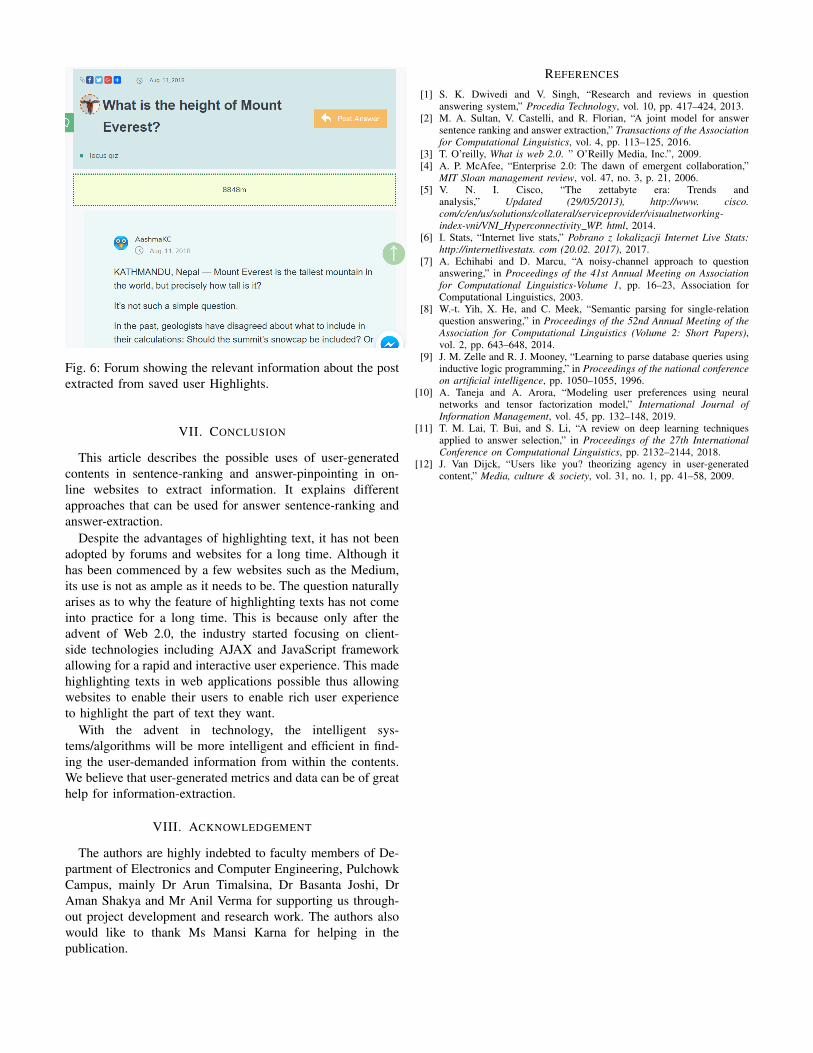
Fig. 6: Forum showing the relevant information about the postextracted from saved user Highlights.
VII. CONCLUSION
This article describes the possible uses of user-generatedcontents in sentence-ranking and answer-pinpointing in on-line websites to extract information. It explains differentapproaches that can be used for answer sentence-ranking andanswer-extraction.
Despite the advantages of highlighting text, it has not beenadopted by forums and websites for a long time. Although ithas been commenced by a few websites such as the Medium,its use is not as ample as it needs to be. The question naturallyarises as to why the feature of highlighting texts has not comeinto practice for a long time. This is because only after theadvent of Web 2.0, the industry started focusing on client-side technologies including AJAX and JavaScript frameworkallowing for a rapid and interactive user experience. This madehighlighting texts in web applications possible thus allowingwebsites to enable their users to enable rich user experienceto highlight the part of text they want.
With the advent in technology, the intelligent sys-tems/algorithms will be more intelligent and efficient in find-ing the user-demanded information from within the contents.We believe that user-generated metrics and data can be of greathelp for information-extraction.
VIII. ACKNOWLEDGEMENT
The authors are highly indebted to faculty members of De-partment of Electronics and Computer Engineering, PulchowkCampus, mainly Dr Arun Timalsina, Dr Basanta Joshi, DrAman Shakya and Mr Anil Verma for supporting us through-out project development and research work. The authors alsowould like to thank Ms Mansi Karna for helping in thepublication.
REFERENCES
[1] S. K. Dwivedi and V. Singh, “Research and reviews in questionanswering system,” Procedia Technology, vol. 10, pp. 417–424, 2013.
[2] M. A. Sultan, V. Castelli, and R. Florian, “A joint model for answersentence ranking and answer extraction,” Transactions of the Associationfor Computational Linguistics, vol. 4, pp. 113–125, 2016.
[3] T. O’reilly, What is web 2.0. ” O’Reilly Media, Inc.”, 2009.[4] A. P. McAfee, “Enterprise 2.0: The dawn of emergent collaboration,”
MIT Sloan management review, vol. 47, no. 3, p. 21, 2006.[5] V. N. I. Cisco, “The zettabyte era: Trends and
analysis,” Updated (29/05/2013), http://www. cisco.com/c/en/us/solutions/collateral/serviceprovider/visualnetworking-index-vni/VNI Hyperconnectivity WP. html, 2014.
[6] I. Stats, “Internet live stats,” Pobrano z lokalizacji Internet Live Stats:http://internetlivestats. com (20.02. 2017), 2017.
[7] A. Echihabi and D. Marcu, “A noisy-channel approach to questionanswering,” in Proceedings of the 41st Annual Meeting on Associationfor Computational Linguistics-Volume 1, pp. 16–23, Association forComputational Linguistics, 2003.
[8] W.-t. Yih, X. He, and C. Meek, “Semantic parsing for single-relationquestion answering,” in Proceedings of the 52nd Annual Meeting of theAssociation for Computational Linguistics (Volume 2: Short Papers),vol. 2, pp. 643–648, 2014.
[9] J. M. Zelle and R. J. Mooney, “Learning to parse database queries usinginductive logic programming,” in Proceedings of the national conferenceon artificial intelligence, pp. 1050–1055, 1996.
[10] A. Taneja and A. Arora, “Modeling user preferences using neuralnetworks and tensor factorization model,” International Journal ofInformation Management, vol. 45, pp. 132–148, 2019.
[11] T. M. Lai, T. Bui, and S. Li, “A review on deep learning techniquesapplied to answer selection,” in Proceedings of the 27th InternationalConference on Computational Linguistics, pp. 2132–2144, 2018.
[12] J. Van Dijck, “Users like you? theorizing agency in user-generatedcontent,” Media, culture & society, vol. 31, no. 1, pp. 41–58, 2009.
Nepali Document Clustering using K-Means, Mini-batchK-Means, and DBSCAN
Aman MaharjanDepartment of CSIT, Tribhuvan University, Kathmandu, Nepal
Tej Bahadur ShahiDepartment of CSIT, Tribhuvan University, Kathmandu, Nepal
Abstract
Automated document clustering is the process of group-ing documents into a small set of meaningful and co-herent collections. This research evaluates K-Means,Mini-batch K-Means and Density-Based Spatial Clus-tering of Applications with Noise (DBSCAN) algo-rithms, in the context of Nepali documents, using fourperformance measures: Homogeneity, Completeness,V-Measure and Silhouette Coefficient. Features extrac-tion is done using Term Frequency – Inverse Docu-ment Frequency (TFIDF). The empirical results showthat Mini-batch K-Means performs better when usingTFIDF. Similarly, in time-constrained environments,the clustering time of Mini-batch K-Means is better thanthe other two algorithms.
Keywords: Clustering, Machine Learning, Nepali Doc-ument Clustering, K-Means, Mini-Batch K-Means, DB-SCAN, TFIDF
1 Introduction
A wide range of research has already been done in thefield of clustering. It is an active field of research dueto its significance in areas like data mining, text mining,information retrieval, statistics, machine learning, biol-ogy, marketing and so on ([1]). The problem of cluster-ing can be very useful in the text domain, where the ob-jects to be clustered can be of different granularities suchas documents, paragraphs, sentences or terms. Cluster-ing is especially useful for organizing documents to im-prove retrieval and support browsing ([2]).
In the context of Nepal, more and more Nepali docu-ments are created and stored in both online and offline
forms each day. Manually clustering them into mean-ingful clusters is both tedious and error-prone. So, auto-matically clustering them using computers is highly de-sirable. As very little research has been done in this areain the past ([3–5]), this study intends to explore threewell-known algorithms in Nepali document clustering.
As Nepali is a complex language, the clustering algo-rithms need to be aware of specific features related tothe language beforehand. This work uses TFIDF repre-senting the features of the documents. It uses three algo-rithms K-Means, Mini-batch K-Means and DBSCAN tocluster the documents and then compares the accuracyand time taken to run the algorithms.
2 Literature Review
The idea of clustering was first used in anthropology by[6]. Later, it was popularized in the field of psychol-ogy by [7] and [8]. It became a major topic in the 1960sand 1970s when the monograph “Principles of Practiceof Numerical Taxonomy”, published by [9], motivatedworldwide research on clustering methods.
Recently, clustering has also been used in browsing doc-uments. One such study, done by [10], noted that doc-ument clustering has not been well received as an in-formation retrieval tool. They objected to the facts thatclustering is too slow for large corpora and clusteringdoes not appreciably improve retrieval. They arguedthat these problems arise only when clustering is used inan attempt to improve conventional search techniques.They presented a document browsing technique that em-ploys document clustering as its primary operation inthat paper as well as a fast (linear time) clustering algo-rithm which support this interactive browsing paradigm.
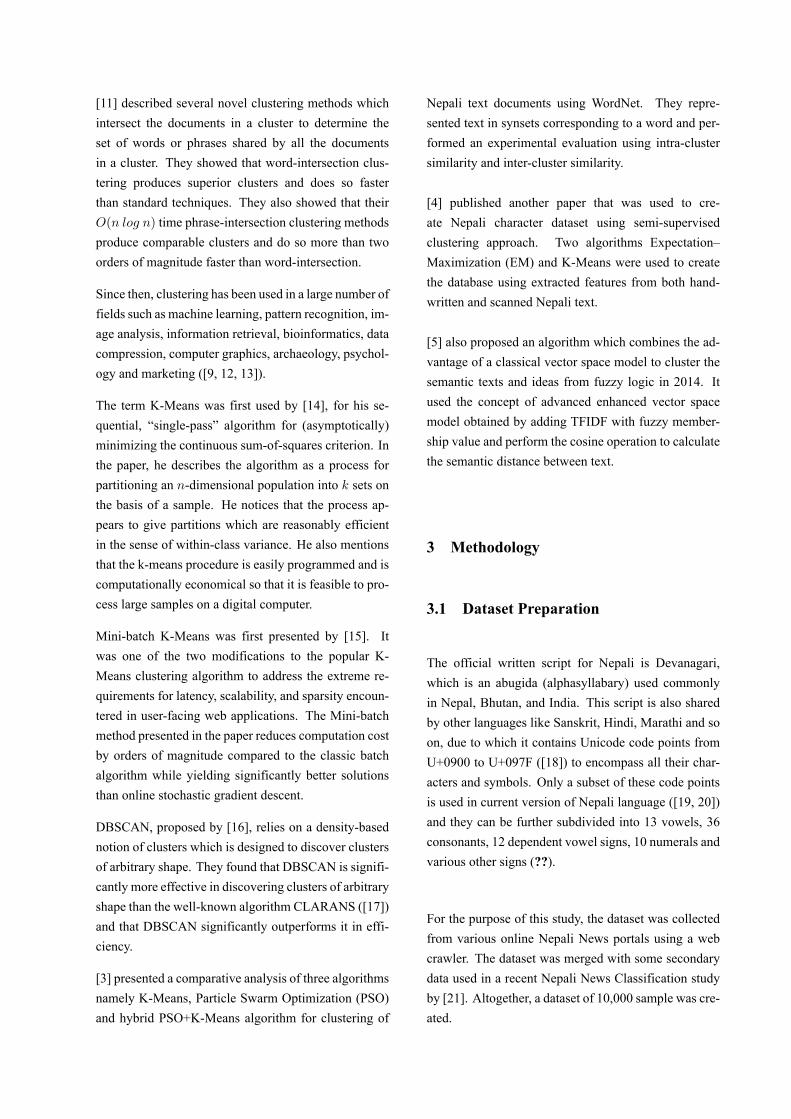
[11] described several novel clustering methods whichintersect the documents in a cluster to determine theset of words or phrases shared by all the documentsin a cluster. They showed that word-intersection clus-tering produces superior clusters and does so fasterthan standard techniques. They also showed that theirO(n log n) time phrase-intersection clustering methodsproduce comparable clusters and do so more than twoorders of magnitude faster than word-intersection.
Since then, clustering has been used in a large number offields such as machine learning, pattern recognition, im-age analysis, information retrieval, bioinformatics, datacompression, computer graphics, archaeology, psychol-ogy and marketing ([9, 12, 13]).
The term K-Means was first used by [14], for his se-quential, “single-pass” algorithm for (asymptotically)minimizing the continuous sum-of-squares criterion. Inthe paper, he describes the algorithm as a process forpartitioning an n-dimensional population into k sets onthe basis of a sample. He notices that the process ap-pears to give partitions which are reasonably efficientin the sense of within-class variance. He also mentionsthat the k-means procedure is easily programmed and iscomputationally economical so that it is feasible to pro-cess large samples on a digital computer.
Mini-batch K-Means was first presented by [15]. Itwas one of the two modifications to the popular K-Means clustering algorithm to address the extreme re-quirements for latency, scalability, and sparsity encoun-tered in user-facing web applications. The Mini-batchmethod presented in the paper reduces computation costby orders of magnitude compared to the classic batchalgorithm while yielding significantly better solutionsthan online stochastic gradient descent.
DBSCAN, proposed by [16], relies on a density-basednotion of clusters which is designed to discover clustersof arbitrary shape. They found that DBSCAN is signifi-cantly more effective in discovering clusters of arbitraryshape than the well-known algorithm CLARANS ([17])and that DBSCAN significantly outperforms it in effi-ciency.
[3] presented a comparative analysis of three algorithmsnamely K-Means, Particle Swarm Optimization (PSO)and hybrid PSO+K-Means algorithm for clustering of
Nepali text documents using WordNet. They repre-sented text in synsets corresponding to a word and per-formed an experimental evaluation using intra-clustersimilarity and inter-cluster similarity.
[4] published another paper that was used to cre-ate Nepali character dataset using semi-supervisedclustering approach. Two algorithms Expectation–Maximization (EM) and K-Means were used to createthe database using extracted features from both hand-written and scanned Nepali text.
[5] also proposed an algorithm which combines the ad-vantage of a classical vector space model to cluster thesemantic texts and ideas from fuzzy logic in 2014. Itused the concept of advanced enhanced vector spacemodel obtained by adding TFIDF with fuzzy member-ship value and perform the cosine operation to calculatethe semantic distance between text.
3 Methodology
3.1 Dataset Preparation
The official written script for Nepali is Devanagari,which is an abugida (alphasyllabary) used commonlyin Nepal, Bhutan, and India. This script is also sharedby other languages like Sanskrit, Hindi, Marathi and soon, due to which it contains Unicode code points fromU+0900 to U+097F ([18]) to encompass all their char-acters and symbols. Only a subset of these code pointsis used in current version of Nepali language ([19, 20])and they can be further subdivided into 13 vowels, 36consonants, 12 dependent vowel signs, 10 numerals andvarious other signs (??).
For the purpose of this study, the dataset was collectedfrom various online Nepali News portals using a webcrawler. The dataset was merged with some secondarydata used in a recent Nepali News Classification studyby [21]. Altogether, a dataset of 10,000 sample was cre-ated.

3.2 Preprocessing
The data in a raw corpus contains many unnecessarycharacters and words that do not contribute much to theclustering process. Filtering out these noisy data speedsup and simultaneously improves the result of clusteranalysis ([21, 22]). The following preprocessing stepswere used on the corpus:
1. Document Sanitization: This step removesall unnecessary characters and symbols usinga whitelist. This includes punctuation marks,HTML tags, zero width joiners, zero width non-joiners etc.
2. Tokenization: This step breaks each individualdocument in the corpus into tokens that can beused directly by later steps.
3. Stop Word Removal: Stop words are the wordswhich have a very high frequency in the corpus.They either do not contribute anything or theircontribution is negligible in differentiating doc-uments and hence are removed before stemming.
4. Stemming: Stemming is the process of removingaffixes from words. Affixes may be either inflec-tional or derivational ([21]). In Nepali, the mean-ing of compound words created using derivationalaffixes are often very different from the root orstem words ([23]). So, this work will focus onlyon stemming inflectional affixes, which reducesthe lexicons to root form without changing theiroverall meaning.
3.3 Text Representation
The text representation of Nepali documents has beendone using TFIDF in this research.
The classic formula for TFIDF is:
wi,j = tfi,j × log(N
dfi
)(1)
where, wi,j is the weight for term i in document j, Nis the number of documents in the corpus, tfi,j is theterm frequency of term i in document j and dfi is thedocument frequency of term i in the corpus.
3.4 Clustering Algorithms
3.4.1 K-Means
The K-Means algorithm performs clustering by sepa-rating samples into k groups, each with equal variancewhile minimizing inertia. The number of clusters shouldbe known before applying this algorithm. It scales wellto a large number of samples and has been used across alarge range of application areas in many different fields.
Mathematically, the K-Means algorithm divides a set S,ofn samples, into k disjoint clustersC, each representedby a meanµi of the samples in the corresponding cluster.The means are commonly called the cluster “centroids”.The centroid generally do not belong to X ([24]).
3.4.2 Mini-batch K-Means
The Mini-batch K-Means is a variant of the K-Means al-gorithm which uses Mini-batches to reduce the compu-tation time, while still attempting to optimize the sameobjective function. Each Mini-batch is a random sub-set of the total samples. The Mini-batch version sig-nificantly reduces the amount of computation requiredto converge to a local solution. It also produces resultsthat are generally only slightly worse than the K-Meansalgorithm ([15]).
3.4.3 DBSCAN
The DBSCAN algorithm is able to find clusters of anyshape as it is guided by the principle that a cluster con-sists of areas of high density separated by areas of lowdensity. There are two parameters to the algorithm,MinPts, and ε. Higher MinPts or lower ε indicateshigher density necessary to form a cluster ([16]).
3.5 Performance Evaluation Parameters
For the purposes of the following discussion, exceptfor silhouette coefficient, a data set comprising N datapoints, and two partitions of these, a set of classes,C = {ci|i = 1, ..., n} and a set of clusters, K =
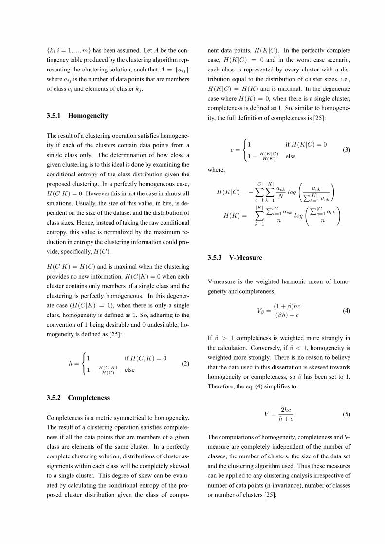
{ki|i = 1, ...,m} has been assumed. Let A be the con-tingency table produced by the clustering algorithm rep-resenting the clustering solution, such that A = {aij}where aij is the number of data points that are membersof class ci and elements of cluster kj .
3.5.1 Homogeneity
The result of a clustering operation satisfies homogene-ity if each of the clusters contain data points from asingle class only. The determination of how close agiven clustering is to this ideal is done by examining theconditional entropy of the class distribution given theproposed clustering. In a perfectly homogeneous case,H(C|K) = 0. However this in not the case in almost allsituations. Usually, the size of this value, in bits, is de-pendent on the size of the dataset and the distribution ofclass sizes. Hence, instead of taking the raw conditionalentropy, this value is normalized by the maximum re-duction in entropy the clustering information could pro-vide, specifically, H(C).
H(C|K) = H(C) and is maximal when the clusteringprovides no new information. H(C|K) = 0 when eachcluster contains only members of a single class and theclustering is perfectly homogeneous. In this degener-ate case (H(C|K) = 0), when there is only a singleclass, homogeneity is defined as 1. So, adhering to theconvention of 1 being desirable and 0 undesirable, ho-mogeneity is defined as [25]:
h =
1 if H(C,K) = 0
1− H(C|K)H(C) else
(2)
3.5.2 Completeness
Completeness is a metric symmetrical to homogeneity.The result of a clustering operation satisfies complete-ness if all the data points that are members of a givenclass are elements of the same cluster. In a perfectlycomplete clustering solution, distributions of cluster as-signments within each class will be completely skewedto a single cluster. This degree of skew can be evalu-ated by calculating the conditional entropy of the pro-posed cluster distribution given the class of compo-
nent data points, H(K|C). In the perfectly completecase, H(K|C) = 0 and in the worst case scenario,each class is represented by every cluster with a dis-tribution equal to the distribution of cluster sizes, i.e.,H(K|C) = H(K) and is maximal. In the degeneratecase where H(K) = 0, when there is a single cluster,completeness is defined as 1. So, similar to homogene-ity, the full definition of completeness is [25]:
c =
1 if H(K|C) = 0
1− H(K|C)H(K) else
(3)
where,
H(K|C) = −|C|∑c=1
|K|∑k=1
ackN
log
(ack∑|K|k=1 ack
)
H(K) = −|K|∑k=1
∑|C|c=1 ackn
log
(∑|C|c=1 ackn
)
3.5.3 V-Measure
V-measure is the weighted harmonic mean of homo-geneity and completeness,
Vβ =(1 + β)hc
(βh) + c(4)
If β > 1 completeness is weighted more strongly inthe calculation. Conversely, if β < 1, homogeneity isweighted more strongly. There is no reason to believethat the data used in this dissertation is skewed towardshomogeneity or completeness, so β has been set to 1.Therefore, the eq. (4) simplifies to:
V =2hc
h+ c(5)
The computations of homogeneity, completeness and V-measure are completely independent of the number ofclasses, the number of clusters, the size of the data setand the clustering algorithm used. Thus these measurescan be applied to any clustering analysis irrespective ofnumber of data points (n-invariance), number of classesor number of clusters [25].
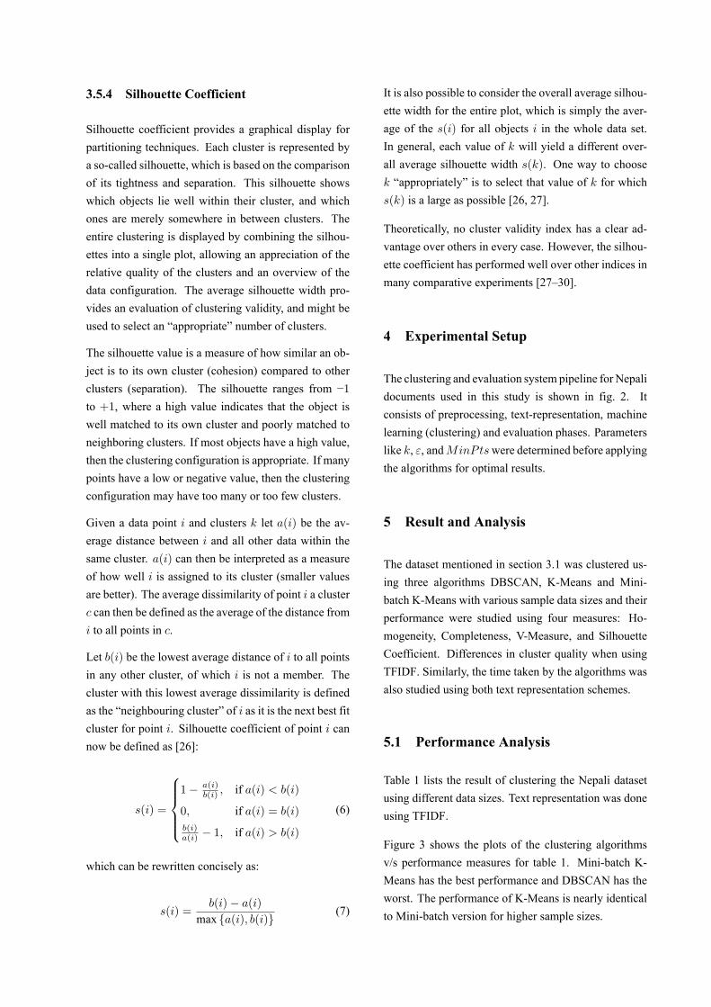
3.5.4 Silhouette Coefficient
Silhouette coefficient provides a graphical display forpartitioning techniques. Each cluster is represented bya so-called silhouette, which is based on the comparisonof its tightness and separation. This silhouette showswhich objects lie well within their cluster, and whichones are merely somewhere in between clusters. Theentire clustering is displayed by combining the silhou-ettes into a single plot, allowing an appreciation of therelative quality of the clusters and an overview of thedata configuration. The average silhouette width pro-vides an evaluation of clustering validity, and might beused to select an “appropriate” number of clusters.
The silhouette value is a measure of how similar an ob-ject is to its own cluster (cohesion) compared to otherclusters (separation). The silhouette ranges from −1to +1, where a high value indicates that the object iswell matched to its own cluster and poorly matched toneighboring clusters. If most objects have a high value,then the clustering configuration is appropriate. If manypoints have a low or negative value, then the clusteringconfiguration may have too many or too few clusters.
Given a data point i and clusters k let a(i) be the av-erage distance between i and all other data within thesame cluster. a(i) can then be interpreted as a measureof how well i is assigned to its cluster (smaller valuesare better). The average dissimilarity of point i a clusterc can then be defined as the average of the distance fromi to all points in c.
Let b(i) be the lowest average distance of i to all pointsin any other cluster, of which i is not a member. Thecluster with this lowest average dissimilarity is definedas the “neighbouring cluster” of i as it is the next best fitcluster for point i. Silhouette coefficient of point i cannow be defined as [26]:
s(i) =
1− a(i)
b(i) , if a(i) < b(i)
0, if a(i) = b(i)
b(i)a(i) − 1, if a(i) > b(i)
(6)
which can be rewritten concisely as:
s(i) =b(i)− a(i)
max {a(i), b(i)}(7)
It is also possible to consider the overall average silhou-ette width for the entire plot, which is simply the aver-age of the s(i) for all objects i in the whole data set.In general, each value of k will yield a different over-all average silhouette width s(k). One way to choosek “appropriately” is to select that value of k for whichs(k) is a large as possible [26, 27].
Theoretically, no cluster validity index has a clear ad-vantage over others in every case. However, the silhou-ette coefficient has performed well over other indices inmany comparative experiments [27–30].
4 Experimental Setup
The clustering and evaluation system pipeline for Nepalidocuments used in this study is shown in fig. 2. Itconsists of preprocessing, text-representation, machinelearning (clustering) and evaluation phases. Parameterslike k, ε, and MinPts were determined before applyingthe algorithms for optimal results.
5 Result and Analysis
The dataset mentioned in section 3.1 was clustered us-ing three algorithms DBSCAN, K-Means and Mini-batch K-Means with various sample data sizes and theirperformance were studied using four measures: Ho-mogeneity, Completeness, V-Measure, and SilhouetteCoefficient. Differences in cluster quality when usingTFIDF. Similarly, the time taken by the algorithms wasalso studied using both text representation schemes.
5.1 Performance Analysis
Table 1 lists the result of clustering the Nepali datasetusing different data sizes. Text representation was doneusing TFIDF.
Figure 3 shows the plots of the clustering algorithmsv/s performance measures for table 1. Mini-batch K-Means has the best performance and DBSCAN has theworst. The performance of K-Means is nearly identicalto Mini-batch version for higher sample sizes.
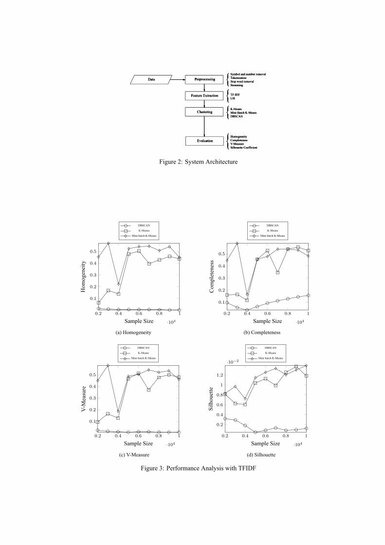
{Symbol and number removalTokenizationStop word removalStemming
Preprocessing
{TF-IDFLSIFeature Extraction
{K-MeansMini-Batch K-MeansDBSCAN
Clustering
{HomogeneityCompletenessV-MeasureSilhouette Coefficient
Evaluation
Data
Figure 2: System Architecture
0.2 0.4 0.6 0.8 1
·104
0.1
0.2
0.3
0.4
0.5
Sample Size
Hom
ogen
eity
DBSCAN
K-Means
Mini-batch K-Means
(a) Homogeneity
0.2 0.4 0.6 0.8 1
·104
0.1
0.2
0.3
0.4
0.5
Sample Size
Com
plet
enes
s
DBSCAN
K-Means
Mini-batch K-Means
(b) Completeness
0.2 0.4 0.6 0.8 1
·104
0.1
0.2
0.3
0.4
0.5
Sample Size
V-M
easu
re
DBSCAN
K-Means
Mini-batch K-Means
(c) V-Measure
0.2 0.4 0.6 0.8 1
·104
0.2
0.4
0.6
0.8
1
1.2
·10−2
Sample Size
Silh
ouet
te
DBSCAN
K-Means
Mini-batch K-Means
(d) Silhouette
Figure 3: Performance Analysis with TFIDF
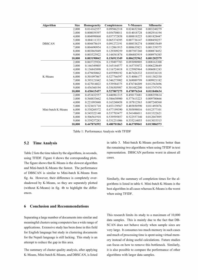
Algorithm Size Homogeneity Completeness V-Measure Silhouette
DBSCAN
2,000 0.014162557 0.095062318 0.024652360 0.0032402793,000 0.008039397 0.054708011 0.014018728 0.0029161944,000 0.004998860 0.037372858 0.008818225 0.0018284475,000 0.004111333 0.065374395 0.007736147 0.0004502576,000 0.004478619 0.091272191 0.008538274 0.0008356497,000 0.004490954 0.112061915 0.008635821 0.0013393758,000 0.003865849 0.129309259 0.007507260 0.0008744529,000 0.003525922 0.144541874 0.006883919 0.00097638510,000 0.003190042 0.156913349 0.006252962 0.001202579
K-Means
2,000 0.065725926 0.159497783 0.093090905 0.0081633003,000 0.166349805 0.165164577 0.165755072 0.0062286494,000 0.136843898 0.116724418 0.125985964 0.0060812435,000 0.479450862 0.455990192 0.467426332 0.0103363186,000 0.501097067 0.527766597 0.514086177 0.0113025307,000 0.395121842 0.346275902 0.369089799 0.0099211828,000 0.427014022 0.539584375 0.476744209 0.0125636969,000 0.456360194 0.556505987 0.501482200 0.01374747610,000 0.438415457 0.527807275 0.478976244 0.011840634
Mini-batch K-Means
2,000 0.453432557 0.446961315 0.450173681 0.0083596143,000 0.568853662 0.586650900 0.577615223 0.0097006664,000 0.221093048 0.163240458 0.187812563 0.0072485605,000 0.523651710 0.453139567 0.485850590 0.0114938766,000 0.538269372 0.477199390 0.505898016 0.0125771017,000 0.545322140 0.537703477 0.541486011 0.0133226218,000 0.506561918 0.539595857 0.522557340 0.0120478959,000 0.539257283 0.531231006 0.535214055 0.01303351510,000 0.447876592 0.480701863 0.463709041 0.013886573
Table 1: Performance Analysis with TFIDF
5.2 Time Analysis
Table 2 lists the time taken by the algorithms, in seconds,using TFIDF. Figure 4 shows the corresponding plots.The figure shows that K-Means is the slowest algorithmand Mini-batch K-Means the fastest. The performanceof DBSCAN is similar to Mini-batch K-Means fromfig. 4a. However, their difference is completely over-shadowed by K-Means, so they are separately plotted(without K-Means) in fig. 4b to highlight the differ-ences.
6 Conclusion and Recommendations
Separating a large number of documents into similar andmeaningful clusters using computers has a wide range ofapplications. Extensive study has been done in this fieldfor English language but study in clustering documentsfor the Nepali language is still lacking. This study is anattempt to reduce the gap in this area.
The summary of cluster quality analysis, after applyingK-Means, Mini-batch K-Means, and DBSCAN, is listed
in table 3. Mini-batch K-Means performs better thanthe remaining two algorithms when using TFIDF in textrepresentation. DBSCAN performs worst in almost allcases.
Similarly, the summary of completion times for the al-gorithms is listed in table 4. Mini-batch K-Means is thebest algorithm in all cases whereas K-Means is the worstwhen using TFIDF.
This research limits its study to a maximum of 10,000data samples. This is mainly due to the fact that DB-SCAN does not behave nicely when sample sizes arevery large. It consumes too much memory in such casesand much of processing time is spent using virtual mem-ory instead of doing useful calculations. Future studiescan focus on how to remove this bottleneck. Similarly,it is also possible to compare the performance of otheralgorithms with larger data samples.
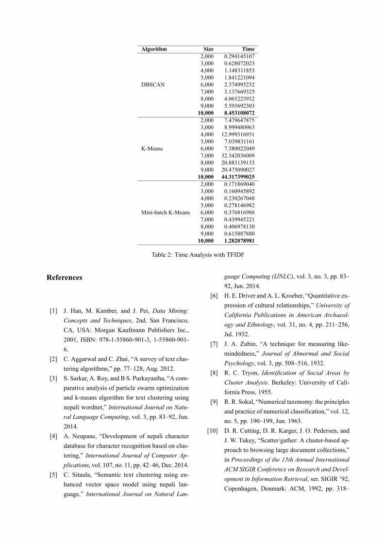
Algorithm Size Time
DBSCAN
2,000 0.2941451073,000 0.6280720234,000 1.1483118535,000 1.8412210946,000 2.3749952327,000 3.1376693258,000 4.0652239329,000 5.59369230310,000 8.453108072
K-Means
2,000 7.4796478753,000 8.9994809634,000 12.9993169315,000 7.0398311616,000 7.3800220497,000 32.3420360098,000 20.8831391339,000 20.47509002710,000 44.317399025
Mini-batch K-Means
2,000 0.1718690403,000 0.1609458924,000 0.2302670485,000 0.2781469826,000 0.3768169887,000 0.4399452218,000 0.4069781309,000 0.61588788010,000 1.282078981
Table 2: Time Analysis with TFIDF
References
[1] J. Han, M. Kamber, and J. Pei, Data Mining:Concepts and Techniques, 2nd. San Francisco,CA, USA: Morgan Kaufmann Publishers Inc.,2001, ISBN: 978-1-55860-901-3, 1-55860-901-6.
[2] C. Aggarwal and C. Zhai, “A survey of text clus-tering algorithms,” pp. 77–128, Aug. 2012.
[3] S. Sarkar, A. Roy, and B S. Purkayastha, “A com-parative analysis of particle swarm optimizationand k-means algorithm for text clustering usingnepali wordnet,” International Journal on Natu-ral Language Computing, vol. 3, pp. 83–92, Jun.2014.
[4] A. Neupane, “Development of nepali characterdatabase for character recognition based on clus-tering,” International Journal of Computer Ap-plications, vol. 107, no. 11, pp. 42–46, Dec. 2014.
[5] C. Sitaula, “Semantic text clustering using en-hanced vector space model using nepali lan-guage,” International Journal on Natural Lan-
guage Computing (IJNLC), vol. 3, no. 3, pp. 83–92, Jun. 2014.
[6] H. E. Driver and A. L. Kroeber, “Quantitative ex-pression of cultural relationships,” University ofCalifornia Publications in American Archaeol-ogy and Ethnology, vol. 31, no. 4, pp. 211–256,Jul. 1932.
[7] J. A. Zubin, “A technique for measuring like-mindedness,” Journal of Abnormal and SocialPsychology, vol. 3, pp. 508–516, 1932.
[8] R. C. Tryon, Identification of Social Areas byCluster Analysis. Berkeley: University of Cali-fornia Press, 1955.
[9] R. R. Sokal, “Numerical taxonomy. the principlesand practice of numerical classification,” vol. 12,no. 5, pp. 190–199, Jun. 1963.
[10] D. R. Cutting, D. R. Karger, J. O. Pedersen, andJ. W. Tukey, “Scatter/gather: A cluster-based ap-proach to browsing large document collections,”in Proceedings of the 15th Annual InternationalACM SIGIR Conference on Research and Devel-opment in Information Retrieval, ser. SIGIR ’92,Copenhagen, Denmark: ACM, 1992, pp. 318–
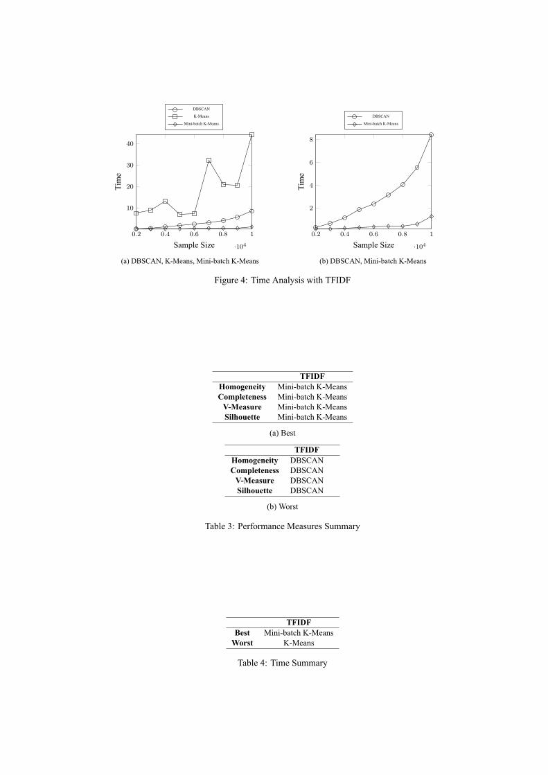
0.2 0.4 0.6 0.8 1
·104
10
20
30
40
Sample Size
Tim
eDBSCAN
K-Means
Mini-batch K-Means
(a) DBSCAN, K-Means, Mini-batch K-Means
0.2 0.4 0.6 0.8 1
·104
2
4
6
8
Sample Size
Tim
e
DBSCAN
Mini-batch K-Means
(b) DBSCAN, Mini-batch K-Means
Figure 4: Time Analysis with TFIDF
TFIDFHomogeneity Mini-batch K-MeansCompleteness Mini-batch K-MeansV-Measure Mini-batch K-MeansSilhouette Mini-batch K-Means
(a) Best
TFIDFHomogeneity DBSCANCompleteness DBSCANV-Measure DBSCANSilhouette DBSCAN
(b) Worst
Table 3: Performance Measures Summary
TFIDFBest Mini-batch K-MeansWorst K-Means
Table 4: Time Summary

329, ISBN: 0-89791-523-2. DOI: 10 . 1145 /133160.133214.
[11] O. Zamir, O. Etzioni, O. Madani, and R. M. Karp,“Fast and intuitive clustering of web documents,”in Proceedings of the Third International Confer-ence on Knowledge Discovery and Data Mining(KDD-97), Newport Beach, California, USA, Au-gust 14-17, 1997, 1997, pp. 287–290.
[12] K. D. Bailey, Typologies and Taxonomies: AnIntroduction to Classification Techniques, M. S.Lewis-Beck, Ed. Thousand Oaks, CA: Sage Pub-lications, 1994. DOI: http://dx.doi.org/10.4135/9781412986397.
[13] H. P. Kriegel, P. Kröger, and A. Zimek, “Cluster-ing high-dimensional data: A survey on subspaceclustering, pattern-based clustering, and corre-lation clustering,” ACM Trans. Knowl. Discov.Data, vol. 3, no. 1, 1:1–1:58, Mar. 2009, ISSN:1556-4681. DOI: 10.1145/1497577.1497578.
[14] J. MacQueen, “Some methods for classificationand analysis of multivariate observations,” inProceedings of the Fifth Berkeley Symposium onMathematical Statistics and Probability, Volume1: Statistics, Berkeley, Calif.: University of Cal-ifornia Press, 1967, pp. 281–297.
[15] D. Sculley, “Web-scale k-means clustering,” inProceedings of the 19th International Conferenceon World Wide Web, ser. WWW ’10, New York,NY, USA: ACM, 2010, pp. 1177–1178, ISBN:978-1-60558-799-8. DOI: 10.1145/1772690.1772862.
[16] M. Ester, H.-P. Kriegel, J. Sander, and X. Xu,“A density-based algorithm for discovering clus-ters a density-based algorithm for discoveringclusters in large spatial databases with noise,” inProceedings of the Second International Confer-ence on Knowledge Discovery and Data Mining,ser. KDD’96, Portland, Oregon: AAAI Press,1996, pp. 226–231.
[17] R. T. Ng and J. Han, “Clarans: A method forclustering objects for spatial data mining,” IEEETransactions on Knowledge and Data Engineer-ing, vol. 14, no. 5, pp. 1003–1016, Sep. 2002,ISSN: 1041-4347. DOI: 10.1109/TKDE.2002.1033770.
[18] Unicode Inc. (2018). The unicode standard 10.0,[Online]. Available: https://www.unicode.
org / charts / PDF / U0900 . pdf (visited on04/10/2018).
[19] N. F. S. Committee. (2018). Nepali font standards(white paper v2), [Online]. Available: https://www.unicode.org/L2/L1999/99235.pdf(visited on 04/10/2018).
[20] B. K. Pokharel, B. Tripathi, K. P. Parajuli, G.Sharma, and H. Bhattarai, Eds., Nepali BrihatShabdakosh, 7th. Kamaladi, Kathmandu, Nepal:Nepal Pragya Pratishthan, 2011.
[21] T. B. Shahi and A. K. Pant, “Nepali news clas-sification using naïve bayes, support vector ma-chines and neural networks,” in 2018 Interna-tional Conference on Communication informa-tion and Computing Technology (ICCICT), Feb.2018, pp. 1–5. DOI: 10.1109/ICCICT.2018.8325883.
[22] N. Haghtalab, “Clustering in the presence ofnoise,” Master’s thesis, University of Water-loo, Waterloo, Ontario, Canada, 2013. [Online].Available: https : / / uwspace . uwaterloo .ca / bitstream / handle / 10012 / 7742 /Haghtalab_Nika.pdf.
[23] I. Shrestha, S. S. Dhakal, and M. Kadariya, “Acomparative study of stemming algorithms fornepali language,” National Student’s Conferenceon Information Technology (NaSCoIT), 2016.
[24] D. Arthur and S. Vassilvitskii, “K-means++: Theadvantages of careful seeding,” in Proceedingsof the Eighteenth Annual ACM-SIAM Symposiumon Discrete Algorithms, ser. SODA ’07, Philadel-phia, PA, USA: Society for Industrial and Ap-plied Mathematics, 2007, pp. 1027–1035, ISBN:978-0-898716-24-5.
[25] A. Rosenberg and J. Hirschberg, “V-measure: Aconditional entropy-based external cluster evalu-ation measure,” in Proceedings of the 2007 JointConference on Empirical Methods in NaturalLanguage Processing and Computational Natu-ral Language Learning, Association for Compu-tational Linguistics, Jan. 2007, pp. 410–420.
[26] P. J. Rousseeuw, “Silhouettes: A graphical aidto the interpretation and validation of clusteranalysis,” Journal of Computational and AppliedMathematics, vol. 20, pp. 53–65, 1987, ISSN:0377-0427. DOI: https : / / doi . org / 10 .1016/0377-0427(87)90125-7.

[27] R. C. de Amorim and C. Hennig, “Recovering thenumber of clusters in data sets with noise featuresusing feature rescaling factors,” Information Sci-ences, vol. 324, pp. 126–145, 2015, ISSN: 0020-0255. DOI: https://doi.org/10.1016/j.ins.2015.06.039.
[28] J. C. Bezdek and N. R. Pal, “Some new indexesof cluster validity,” IEEE Transactions on Sys-tems, Man, and Cybernetics, Part B (Cybernet-ics), vol. 28, no. 3, pp. 301–315, Jun. 1998, ISSN:1083-4419. DOI: 10.1109/3477.678624.
[29] O. Arbelaitz, I. Gurrutxaga, J. Muguerza, J. M.Pérez, and I. Perona, “An extensive comparativestudy of cluster validity indices,” Pattern Recog-nition, vol. 46, no. 1, pp. 243–256, 2013, ISSN:0031-3203. DOI: https : / / doi . org / 10 .1016/j.patcog.2012.07.021.
[30] K. S.P.M. J. van der Laan, “A method to iden-tify significant clusters in gene expression data,”in Proceedings of the 6th World Multiconferenceon Systemics, Cybernetics and Informatics, Or-lando, USA: Inpress, 2002, pp. 318–325.
Performance Analysis Between Haar and Daubechies Discrete Wavelet Transform in Digital Watermarking
Rajan Kusi Nepal College of Information Technology
Lalitpur, Nepal
Dr. Sanjib Panday
,Assoc. Professor, IoE, Pulchowk Campus Lalitpur, Nepal
Abstract— In this paper, the cover image is embedded
with watermark image and from the watermarked image
and the watermark image has been extracted by using
haar and daubechies discrete wavelet transform based
digital watermarking by using MATLAB Simulation
software and also performance of these watermarking has
been evaluated using different performance metrics they
are mean square error (MSE), peak signal to noise ratio
(PSNR), structural similarity index measure (SSIM) and
correlation coefficient (CRC). In the simulation result, we
found that daubechies wavelet transform give better
performance over haar wavelet transform in terms of
PSNR, MSE, SSIM and CRC.
Keywords— haar discrete wavelet transform, daubechies
discrete wavelet transform, watermark image.
I. INTRODUCTION
With advancements in digital communication
technology and the growth of computer power and
storage, the difficulties in ensuring individuals’ privacy
become increasingly challenging. The degrees to which
individuals appreciate privacy differ from one person to
another. Various methods have been investigated and
developed to protect personal privacy [1].
Watermarking is a technology that provides data
security, authentication and integrity and also provides
copyright protection for digital media. Watermarking
process mainly consists of two modules, watermark
embedding module and watermark extraction and
detection module. The main focus of watermarking
technology is to embed secret information or signal into
digital images, video and audio etc. After embedding the
information is detected and extracted and extracted
information reveals real identity of media or owner [2].
Digital watermarking is the act of hiding a message
related to a digital signal (i.e. an image, song, and video)
within the signal itself. It is a concept closely related to
steganography, in that they both hide a message inside a
digital signal. However, what separates them is their
goal. Watermarking tries to hide a message related to the
actual content of the digital signal, while in
steganography the digital signal has no relation to the
message, and it is merely used as a cover to hide its
existence [3].
Wavelet based image watermarking is gaining more
popularity because of its similarity with the human
visual system, and various digital watermarking
techniques with haar wavelet transform. It is necessary
to provide security along with resistant to geometric
distortion and noise also better PSNR. Block diagram of
digital watermarking shown in figure 1.
Fig. 1. Basic Block Diagram of Digital Watermarking
This paper is organized as follows, description of
haar and daubechies discrete wavelet transform is
presented in Section II and simulation results are
described in Section III. Finally, conclusion is stated in
Section IV.
II. HAAR AND DAUBECHIES DISCRETE
WAVELET TRANSFORM
There are various techniques in implementing
digital watermarking. These techniques are commonly
categorized in terms of working domain i.e. spatial
domain or transform domain. In spatial domain, pixel
luminance and chrominance values are modified to
embed the watermark for example Least Significant Bit
(LSB), correlation based and patchwork techniques.
While in transform domain, the media content
undergoes mathematical transformation before
watermark embedding is done for example using
Discrete Fourier Transform (DFT), Discrete Cosine
Transform (DCT) and Discrete Wavelet Transform
(DWT)[4]. However, DWT has been used more
frequently in digital image watermarking due to its
time/frequency decomposition characteristics, which
resemble to the theoretical models of the human visual
system.
Waterma
rk Image
Cover
Image
Embeddi
ng
Function
Waterma
rked
Image
Extractio
n
Function
Waterm
ark
Image

Wavelet Domain is a promising domain for
watermark embedding. Wavelet refers to small waves.
Discrete wavelet transformation is based on small
waves of limited duration and varying frequency. This
is a frequency domain technique in which firstly cover
image is transformed into frequency domain and then
its frequency coefficients are modified in accordance
with the transformed coefficients of the watermark and
watermarked image is obtained which is very much
robust. DWT decomposed image hierarchically,
providing both spatial and frequency description of the
image. It decomposes an image in basically three spatial
directions i.e. horizontal, vertical and diagonal in result
separating into four different components namely LL,
LH, HL and HH. Here first letter refers to applying
either low pass frequency operation or high pass
frequency operations to the rows and the second refers
to the filter applied to the columns of the cover image.
LL level is the lowest resolution level which consist of
the approximation part of the cover image and rest three
levels i.e., LH, HL, HH give the detailed information of
the cover image. DWT decomposition of image is as
shown in figure 2.
Fig. 2. DWT Decomposition of the Image
A. Haar Discrete Wavelet Transform Haar is the simplest and very fast wavelet transform.
Haar matrix is sequentially ordered. Inma thematics, the
Haar wavelet is a sequence of rescaled ―square-shaped
functions. The wavelet theorems are most popular
methods of image processing, de-noising and
compression. Considering that the Haar functions are
the simplest wavelets, these forms are used in many
methods of discrete image transforms and processing.
The Haar wavelet transform has a number of
advantages such as it is conceptually fast, simple,
memory efficient, since it can be calculated in place
without a temporary array.
The Haar wavelet also has limitations. In generating
each of averages for the next level and each set of
coefficients, the Haar transform performs an average and
difference on a pair of values. Then the algorithm shifts
over by two values and calculates another average and
difference on the next pair. The high frequency
coefficient spectrum should reflect all high frequency
changes. The Haar window is only two elements wide. If
a big change takes place from an even value to an odd
value, the change will not be reflected in the high
frequency coefficients.
In the process of watermark embedding, a watermark
image is embedded in the cover image. In order to
embed a watermark in an image Haar wavelet is used as
mother wavelet.
B. Daubechies Discrete Wavelet Transform Daubechies wavelets are the most popular wavelets.
They represent the foundations of wavelet signal
processing and are used in various applications. These
are also called Maxflat wavelets as their frequency
responses have maximum flatness at frequencies 0 and
π. The Daubechies wavelet transforms are defined in the
same way as the Haar wavelet transform by computing
running averages and differences via scalar products
with scaling signals and wavelets the only difference
between them consists in how these scaling signals and
wavelets are defined. For the Daubechies wavelet
transforms, the scaling signals and wavelets have
slightly longer supports, i.e., they produce averages and
differences using just a few more values from the signal.
This slight change, however, provides a tremendous
improvement in the capabilities of these new transforms.
The names of the Daubechies family wavelets are
written dbN, where N is the order, and db the "surname"
of the wavelet. db1 is same as Haar wavelet, generally
these are considered as same wavelet.
In the process of watermark embedding, an
watermark image is embedded in the cover image. In
order to embed a watermark in an image Daubechies
wavelet is used as mother wavelet. The watermark
embedding and extraction process using Daubechies
wavelet transform is as illustrated in following block
diagram 3.
Fig. 3. Embedding Process in Daubechies Wavelet Transform
Watermarked
Image
Apply IDWT
DaubechiesTransform
Cover Image
Apply Daubechies Haar
Transform
Embed Process in Daubechies DWT coefficient
Watermark Image
XOR pixel value with
secret key
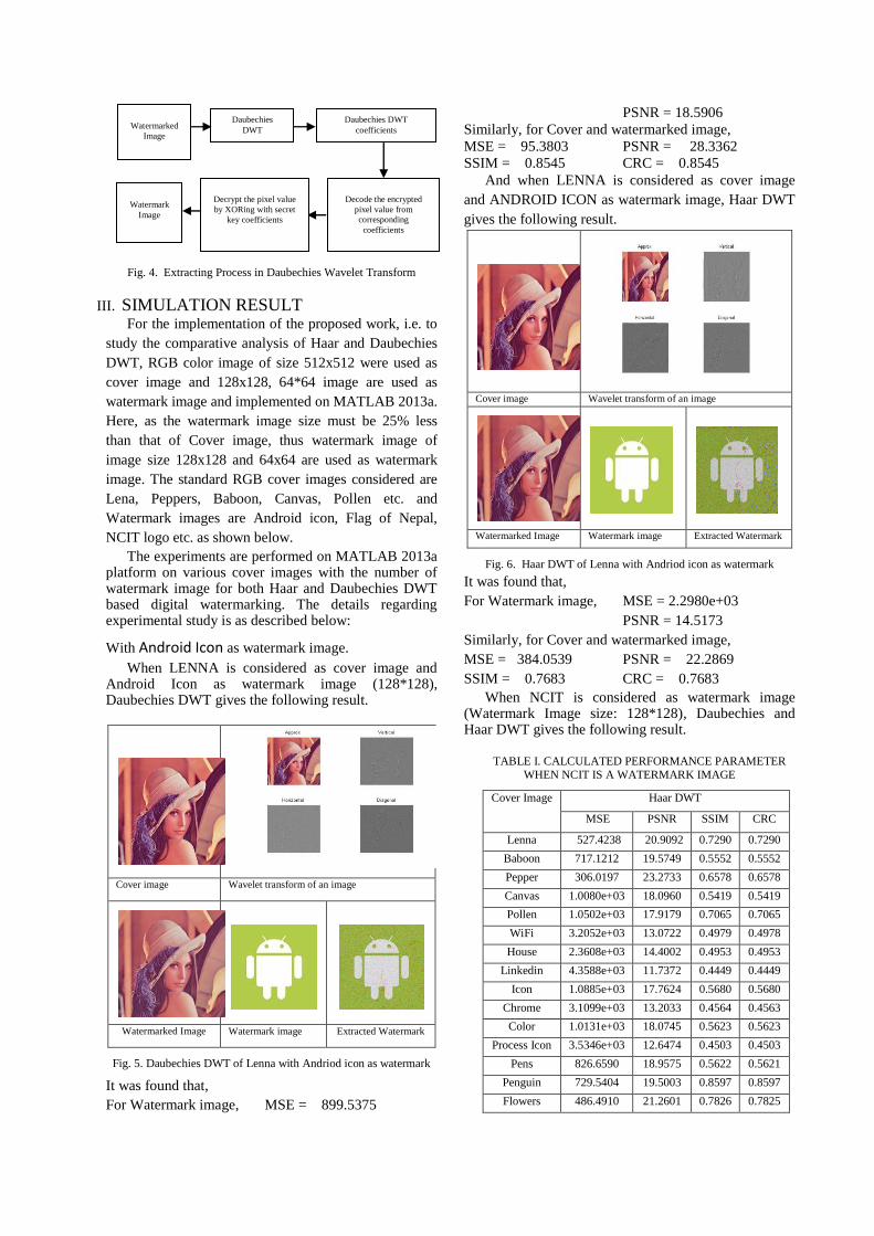
Fig. 4. Extracting Process in Daubechies Wavelet Transform
III. SIMULATION RESULT For the implementation of the proposed work, i.e. to
study the comparative analysis of Haar and Daubechies
DWT, RGB color image of size 512x512 were used as
cover image and 128x128, 64*64 image are used as
watermark image and implemented on MATLAB 2013a.
Here, as the watermark image size must be 25% less
than that of Cover image, thus watermark image of
image size 128x128 and 64x64 are used as watermark
image. The standard RGB cover images considered are
Lena, Peppers, Baboon, Canvas, Pollen etc. and
Watermark images are Android icon, Flag of Nepal,
NCIT logo etc. as shown below.
The experiments are performed on MATLAB 2013a platform on various cover images with the number of watermark image for both Haar and Daubechies DWT based digital watermarking. The details regarding experimental study is as described below:
With Android Icon as watermark image.
When LENNA is considered as cover image and Android Icon as watermark image (128*128), Daubechies DWT gives the following result.
Cover image Wavelet transform of an image
Watermarked Image Watermark image Extracted Watermark
Fig. 5. Daubechies DWT of Lenna with Andriod icon as watermark
It was found that,
For Watermark image, MSE = 899.5375
PSNR = 18.5906
Similarly, for Cover and watermarked image,
MSE = 95.3803 PSNR = 28.3362
SSIM = 0.8545 CRC = 0.8545
And when LENNA is considered as cover image
and ANDROID ICON as watermark image, Haar DWT
gives the following result.
Cover image Wavelet transform of an image
Watermarked Image Watermark image Extracted Watermark
Fig. 6. Haar DWT of Lenna with Andriod icon as watermark
It was found that,
For Watermark image, MSE = 2.2980e+03
PSNR = 14.5173
Similarly, for Cover and watermarked image,
MSE = 384.0539 PSNR = 22.2869
SSIM = 0.7683 CRC = 0.7683
When NCIT is considered as watermark image (Watermark Image size: 128*128), Daubechies and Haar DWT gives the following result.
TABLE I. CALCULATED PERFORMANCE PARAMETER
WHEN NCIT IS A WATERMARK IMAGE
Cover Image Haar DWT
MSE PSNR SSIM CRC
Lenna 527.4238 20.9092 0.7290 0.7290
Baboon 717.1212 19.5749 0.5552 0.5552
Pepper 306.0197 23.2733 0.6578 0.6578
Canvas 1.0080e+03 18.0960 0.5419 0.5419
Pollen 1.0502e+03 17.9179 0.7065 0.7065
WiFi 3.2052e+03 13.0722 0.4979 0.4978
House 2.3608e+03 14.4002 0.4953 0.4953
Linkedin 4.3588e+03 11.7372 0.4449 0.4449
Icon 1.0885e+03 17.7624 0.5680 0.5680
Chrome 3.1099e+03 13.2033 0.4564 0.4563
Color 1.0131e+03 18.0745 0.5623 0.5623
Process Icon 3.5346e+03 12.6474 0.4503 0.4503
Pens 826.6590 18.9575 0.5622 0.5621
Penguin 729.5404 19.5003 0.8597 0.8597
Flowers 486.4910 21.2601 0.7826 0.7825
Watermarked
Image
Daubechies
DWT
Daubechies DWT
coefficients
Watermark
Image
Decode the encrypted
pixel value from
corresponding
coefficients
Decrypt the pixel value
by XORing with secret
key coefficients
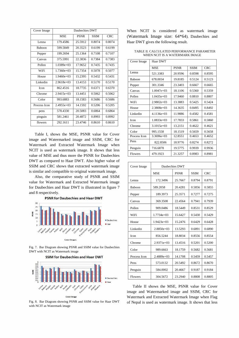
Cover Image Daubechies DWT
MSE PSNR SSIM CRC
Lenna 179.4586 25.5912 0.8074 0.8074
Baboon 599.5849 20.3523 0.6199 0.6199
Pepper 199.2694 25.1364 0.7108 0.7107
Canvas 375.5991 22.3836 0.7384 0.7383
Pollen 1.0389e+03 17.9652 0.7435 0.7435
WiFi 1.7360e+03 15.7354 0.5078 0.5077
House 1.9460e+03 15.2395 0.5432 0.5431
Linkedin 2.9618e+03 13.4153 0.5170 0.5170
Icon 862.4516 18.7735 0.6371 0.6370
Chrome 2.9415e+03 13.4451 0.5062 0.5062
Color 993.6883 18.1583 0.5686 0.5686
Process Icon 2.4955e+03 14.1592 0.5206 0.5205
pens 578.4330 20.5083 0.6864 0.6864
pinguin 581.2461 20.4872 0.8993 0.8992
flowers 292.1611 23.4746 0.8610 0.8610
Table I, shows the MSE, PSNR value for Cover
image and Watermarked image and SSIM, CRC for
Watermark and Extracted Watermark Image when
NCIT is used as watermark image. It shows that less
value of MSE and thus more the PSNR for Daubechies
DWT as compared to Haar DWT. Also higher value of
SSIM and CRC shows that extracted watermark image
is similar and compatible to original watermark image.
Also, the comparative study of PSNR and SSIM
value for Watermark and Extracted Watermark image
for Daubechies and Haar DWT is illustrated in figure 7
and 8 respectively.
Fig. 7. Bar Diagram showing PSNR and SSIM value for Daubechies
DWT with NCIT as Watermark image
Fig. 8. Bar Diagram showing PSNR and SSIM value for Haar DWT
with NCIT as Watermark image
When NCIT is considered as watermark image
(Watermark Image size: 64*64), Daubechies and
Haar DWT gives the following result.
TABLE II. CALCULATED PERFORMANCE PARAMETER
WHEN NCIT IS A WATERMARK IMAGE
Cover Image Haar DWT
MSE PSNR SSIM CRC
Lenna 521.3383 20.9596 0.8598 0.8595
Baboon 678.0034 19.8185 0.5124 0.5123
Pepper 301.3346 23.3403 0.6667 0.6665
Canvas 1.0047e+03 18.1106 0.5360 0.5359
Pollen 1.0435e+03 17.9460 0.8810 0.8807
WiFi 2.9802e+03 13.3883 0.5425 0.5424
House 2.3808e+03 14.3635 0.8495 0.8492
Linkedin 4.1136e+03 11.9886 0.4582 0.4581
Icon 1.0833e+03 17.7833 0.5861 0.5860
Chrome 3.1015e+03 13.2151 0.4622 0.4621
Color 995.1558 18.1519 0.5659 0.5658
Process Icon 3.3696e+03 12.8551 0.4653 0.4652
Pens 822.8506 18.9776 0.8274 0.8272
Penguin 716.6878 19.5775 0.9939 0.9936
Flowers 479.1923 21.3257 0.8983 0.8981
Cover Image Daubechies DWT
MSE PSNR SSIM CRC
Lenna 172.3496 25.7667 0.8794 0.8791
Baboon 589.2058 20.4281 0.5856 0.5855
Pepper 189.3973 25.3571 0.7277 0.7275
Canvas 369.3508 22.4564 0.7941 0.7939
Pollen 909.0486 18.5449 0.8531 0.8529
WiFi 1.7734e+03 15.6427 0.5430 0.5429
House 1.9423e+03 15.2476 0.6429 0.6428
Linkedin 2.8850e+03 13.5293 0.6891 0.6890
Icon 856.5244 18.8034 0.8556 0.8554
Chrome 2.9371e+03 13.4516 0.5201 0.5200
Color 989.6663 18.1759 0.5682 0.5681
Process Icon 2.4889e+03 14.1708 0.5459 0.5457
Pens 573.0132 20.5492 0.8672 0.8670
Penguin 584.0002 20.4667 0.9187 0.9184
Flowers 304.5672 23.2940 0.8808 0.8805
Table II shows the MSE, PSNR value for Cover
image and Watermarked image and SSIM, CRC for
Watermark and Extracted Watermark Image when Flag
of Nepal is used as watermark image. It shows that less
value of MSE and thus more the PSNR for Daubechies
DWT as compared to Haar DWT. Also higher value of
SSIM and CRC shows that extracted watermark image
is similar and compatible to original watermark image.
Also, the comparative study of PSNR and SSIM
value for Watermark and Extracted Watermark image
for Daubechies and Haar DWT is shown in figure 9 and
10.
Fig. 9. Bar Diagram showing PSNR and SSIM value for Daubechies
DWT with NCIT as Watermark image
Fig. 10. Bar Diagram showing PSNR and SSIM value for Haar DWT
with Robot as Watermark image
IV. CONCLUSION This paper, mainly focused on invisible
watermarking that provides a comprehensive and robust
algorithm that embeds and extracts watermark image
effectively. The Wavelet transform of various Cover
images with different watermark image has been
performed and to evaluate the performance of the Haar
and Daubechies DWT based digital watermarking,
performance metrics: MSE, PSNR, SSIM and CRC
were calculated. The above experiments show that
Daubechies DWT gives less MSE and thus more PSNR
compared to Haar DWT. With the higher value of
PSNR that defines the imperceptibility so we can say
that the cover image and watermarked image are
visually same. In terms of SSIM and CRC, Daubechies
DWT have larger value, shows the high similarity
between the original watermark and extracted
watermark than that of Haar DWT. By human visual
system it seems that Daubechies gave best result. Also
it has been observed that performance metrics for 64*64
is better than 128*128 watermark image which shows
that less the image size better the performance.
Thus it can be concluded that performance of
Daubechies DWT is better than Haar DWT in digital
watermarking.
REFERENCES
[1] Abbas Cheddad, “A New Image Steganography
Algorithm”, 2009
[2] Manish Deoli, Rohan Verma, International Journal
of Advanced Research in Computer Science and
Software Engineering, 2016, “A Comparative
Analysis of Popular Digital Image Watermarking
Techniques”
[3] Yusnita Binti Yusof, 2009, “Improved digital
image watermarking using discrete wavelet
transform”
[4] Nidhi Bisla, Prachi Chaudhary, International
Journal of Advanced Research in Computer
Science and Software Engineering, 2013,
“Comparative Study of DWT and DWT-SVD
Image Watermarking Techniques”
[5] Pravin M. Pithiya, H.L.Desai, International Journal
of Engineering Research and Development, 2013,
“DWT Based Digital Image Watermarking, De-
Watermarking & Authentication”
[6] Khalid A. Darabkh, Journal of Software
Engineering and Applications, 2014
,“Imperceptible and Robust DWT-SVD-Based
Digital Audio Watermarking Algorithm”
[7] Anuradha , Rudresh Pratap Singh, International
Journal of Electronics and Computer Science
Engineering, ISSN- 2277-1956 , “DWT Based
Watermarking Algorithm using Haar Wavelet”
[8] Pravin M. Pithiya, H.L.Desai, International Journal
of Recent Development in Engineering and
Technology, 2014 , “Optimized Image
Steganography using Discrete Wavelet Transform
(DWT)”

Performance Analysis of Electricity Demand withMeteorological Parameters for Japan
Kamal Chapagain∗, Tomonori Sato †, Somsak Kittipiyakul∗∗Sirindhorn International Institute of Technology, Thammasat University, Pathumthani, Thailand
†Graduate School of Environmental Science, Hokkaido University, Sapporo, JapanCorresponding author: [email protected]
Abstract—The quality of short term electricity demand fore-casting is essential for all the energy market players for operationand trading activities. Electricity demand is significantly affectedby non linear factors such as climatic condition, calendar andother seasonality have been widely reported in literature. Thispaper considers parsimonious forecasting models to explainthe importance of meteorological parameters for the hourlyelectricity demand forecasting. Many researchers include onlytemperature as a major weather factor because it directly influ-ences electricity demand, however other meteorological factorssuch as relative humidity, wind speed etc. are rarely includedin literature. Therefore, the main purpose of this study is to in-vestigate the impact of meteorological variability such as relativehumidity, wind speed, solar radiation etc. for short term demandforecasting and analyzed it quantitatively. We demonstrate threedifferent multiple linear models including auto-regressive movingaverage ARMA (2,6) models with and without some exogenousweather variables to compare the performances for HokkaidoPrefecture, Japan. We applied Bayesian approach to estimatethe weight of each parameters with Gibbs sampling and resultsshow overall improvement of mean absolute percentage error(MAPE) performance by 0.015%.
I. INTRODUCTION
Short term electricity demand forecasting is importantfor all stakeholder of electricity- such as market operator,electricity generators, electricity retailers and ultimately forgeneral people. For market operator, forecasting is crucial forscheduling and dispatch of generators capacity. For electricitygenerators, strategic choice involved in bidding and re-biddingof capacity depends on demand forecast[3]. For, electricityretailer, demand forecasting affects the decisions about thebalance between hedging spot acquisition of electricity, andfinally these actions helps for general people due to consistentenergy supplies without black out and possibly minimum cost.
Various models are discussed in literature and pay atten-tion for better performance. Electricity demand in Japan hasstrong time correlation with lagged dependent variable suchas Ohtsuka Y. et al. [8], and therefore there are severalpapers that relate with ARMA time series structure. OhtsukaY. et al. have proposed Bayesian estimation procedures forunivariate ARMA and got good performance as well. Sinceeach model has its own strength and weakness, we havedeveloped multiple equation model accounting correlated erroras hybrid model. As distinct from previous studies, we em-ploy two stage estimation of multiple linear regression MLRARMA(2,6) model. First stage, we get point estimation values
of parameters using ordinary least square (OLS) technique andrefine these estimation using Bayesian technique in secondstage.
To develop model several factors that directly or indirectlyinfluence on electricity demand have to take in account.For example- weather, calendar, and historical demand data.Impact of weather variables on electric power demand inEngland, Australia, Jordan and many more regions are foundin literature, but their focus is on the affect of temperature.Failure of power supply in 1995 due to excessive hot, andcorresponding increase of electricity demand in Malaysia.Such increment of demand is possible if temperature lowerssignificantly. Countries having cold regions have the peakdemand in the summer are usually lower compared to the peakdemands of winter. This indicates that human activities duringwinter season is higher. Various weather variables can beconsidered for demand forecasting: temperature and humidityare the most commonly used, but wind, radiation and cloudcover are often excluded. The affect of meteorological factorssuch as temperature, humidity, solar radiation, precipitation,and wind speed varies according to the season and hence varieselectricity demand significantly. However, most of the paperexclude other factors and include only temperature for theiranalysis.
Among various approaches for predicting future data, wecan generalize into two types of estimates. i) point estimate-single valued forecast, and ii) probabilistic estimate- whereeach parameters are treated as random variable and severalpossible values for the future demand is predicted. The mainadvantage of probabilistic forecast is that it contains additionalinformation in terms of uncertainty. This paper employ twostage for estimation. In first stage, the point estimated valuesobtained from OLS is considered as prior information forBayesian and in next stage, these parameters are used asrandom variable for Markov Chain Monte Carlo (MCMC)and obtained the final values in terms of distributions forprobabilistic forecast. Finally, forecasting the next day demandis in terms of mean, median and 60 percentile value.
II. METHODOLOGY
A. Description of data
We have played with the hourly electricity demand datafrom Jan 1, 2013 until December 31, 2015 for HokkaidoPrefecture provided by Hokkaido Electric Power Company
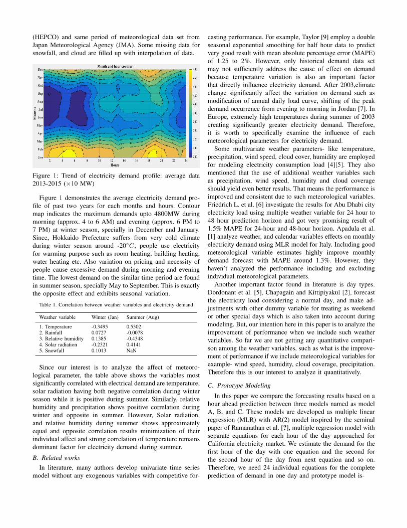
(HEPCO) and same period of meteorological data set fromJapan Meteorological Agency (JMA). Some missing data forsnowfall, and cloud are filled up with interpolation of data.
Figure 1: Trend of electricity demand profile: average data2013-2015 (×10 MW)
Figure 1 demonstrates the average electricity demand pro-file of past two years for each months and hours. Contourmap indicates the maximum demands upto 4800MW duringmorning (approx. 4 to 6 AM) and evening (approx. 6 PM to7 PM) at winter season, specially in December and January.Since, Hokkaido Prefecture suffers from very cold climateduring winter season around -20◦C, people use electricityfor warming purpose such as room heating, building heating,water heating etc. Also variation on pricing and necessity ofpeople cause excessive demand during morning and eveningtime. The lowest demand on the similar time period are foundin summer season, specially May to September. This is exactlythe opposite effect and exhibits seasonal variation.
Table 1. Correlation between weather variables and electricity demand
Weather variable Winter (Jan) Summer (Aug)
1. Temperature -0.3495 0.53022. Rainfall 0.0727 -0.00783. Relative humidity 0.1385 -0.43484. Solar radiation -0.2321 0.41415. Snowfall 0.1013 NaN
Since our interest is to analyze the affect of meteoro-logical parameter, the table above shows the variables mostsignificantly correlated with electrical demand are temperature,solar radiation having both negative correlation during winterseason while it is positive during summer. Similarly, relativehumidity and precipitation shows positive correlation duringwinter and opposite in summer. However, Solar radiation,and relative humidity during summer shows approximatelyequal and opposite correlation results minimization of theirindividual affect and strong correlation of temperature remainsdominant factor for electricity demand during summer.
B. Related worksIn literature, many authors develop univariate time series
model without any exogenous variables with competitive for-
casting performance. For example, Taylor [9] employ a doubleseasonal exponential smoothing for half hour data to predictvery good result with mean absolute percentage error (MAPE)of 1.25 to 2%. However, only historical demand data setmay not sufficiently address the cause of effect on demandbecause temperature variation is also an important factorthat directly influence electricity demand. After 2003,climatechange significantly affect the variation on demand such asmodification of annual daily load curve, shifting of the peakdemand occurrence from evening to morning in Jordan [7]. InEurope, extremely high temperatures during summer of 2003creating significantly greater electricity demand. Therefore,it is worth to specifically examine the influence of eachmeteorological parameters for electricity demand.
Some multivariate weather parameters- like temperature,precipitation, wind speed, cloud cover, humidity are employedfor modeling electricity consumption load [4][5]. They alsomentioned that the use of additional weather variables suchas precipitation, wind speed, humidity and cloud coverageshould yield even better results. That means the performance isimproved and consistent due to such meteorological variables.Friedrich L. et al. [6] investigate the results for Abu Dhabi cityelectricity load using multiple weather variable for 24 hour to48 hour prediction horizon and got very promising result of1.5% MAPE for 24-hour and 48-hour horizon. Apadula et al.[1] analyze weather, and calendar variables effects on monthlyelectricity demand using MLR model for Italy. Including goodmeteorological variable estimates highly improve monthlydemand forecast with MAPE around 1.3%. However, theyhaven’t analyzed the performance including and excludingindividual meteorological parameters.
Another important factor found in literature is day types.Dordonant et al. [5], Chapagain and Kittipiyakul [2], forecastthe electricity load considering a normal day, and make ad-justments with other dummy variable for treating as weekendor other special days which is also taken into account duringmodeling. But, our intention here in this paper is to analyze theimprovement of performance when we include such weathervariables. So far we are not getting any quantitative compari-son among the weather variables, such as what is the improve-ment of performance if we include meteorological variables forexample- wind speed, humidity, cloud coverage, precipitation.Therefore this is our interest to analyze it quantitatively.
C. Prototype Modeling
In this paper we compare the forecasting results based on ahour ahead prediction between three models named as modelA, B, and C. These models are developed as multiple linearregression (MLR) with AR(2) model inspired by the seminalpaper of Ramanathan et al. [?], multiple regression model withseparate equations for each hour of the day approached forCalifornia electricity market. We estimate the demand for thefirst hour of the day with one equation and the second forthe second hour of the day from next equation and so on.Therefore, we need 24 individual equations for the completeprediction of demand in one day and prototype model is-
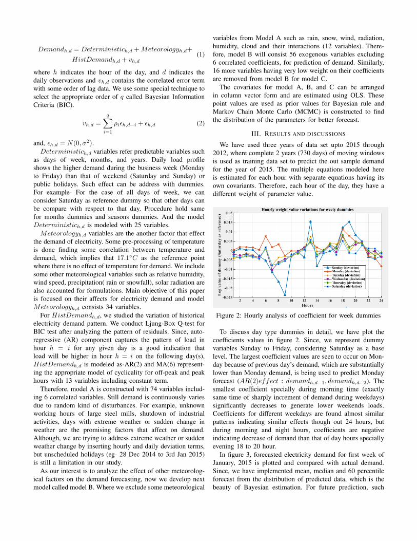
Demandh,d = Deterministich,d +Meteorologyh,d+
HistDemandh,d + vh,d(1)
where h indicates the hour of the day, and d indicates thedaily observations and vh,d contains the correlated error termwith some order of lag data. We use some special technique toselect the appropriate order of q called Bayesian InformationCriteria (BIC).
vh,d =
q∑i=1
ρiεh,d−i + εh,d (2)
and, εh,d = N(0, σ2).Deterministich,d variables refer predictable variables such
as days of week, months, and years. Daily load profileshows the higher demand during the business week (Mondayto Friday) than that of weekend (Saturday and Sunday) orpublic holidays. Such effect can be address with dummies.For example- For the case of all days of week, we canconsider Saturday as reference dummy so that other days canbe compare with respect to that day. Procedure hold samefor months dummies and seasons dummies. And the modelDeterministich,d is modeled with 25 variables.Meteorologyh,d variables are the another factor that effect
the demand of electricity. Some pre-processing of temperatureis done finding some correlation between temperature anddemand, which implies that 17.1◦C as the reference pointwhere there is no effect of temperature for demand. We includesome other meteorological variables such as relative humidity,wind speed, precipitation( rain or snowfall), solar radiation arealso accounted for formulations. Main objective of this paperis focused on their affects for electricity demand and modelMeteorologyh,d consists 34 variables.
For HistDemandh,d, we studied the variation of historicalelectricity demand pattern. We conduct Ljung-Box Q-test forBIC test after analyzing the pattern of residuals. Since, auto-regressive (AR) component captures the pattern of load inhour h = i for any given day is a good indication thatload will be higher in hour h = i on the following day(s),HistDemandh,d is modeled as-AR(2) and MA(6) represent-ing the appropriate model of cyclicality for off-peak and peakhours with 13 variables including constant term.
Therefore, model A is constructed with 74 variables includ-ing 6 correlated variables. Still demand is continuously variesdue to random kind of disturbances. For example, unknownworking hours of large steel mills, shutdown of industrialactivities, days with extreme weather or sudden change inweather are the promising factors that affect on demand.Although, we are trying to address extreme weather or suddenweather change by inserting hourly and daily deviation terms,but unscheduled holidays (eg- 28 Dec 2014 to 3rd Jan 2015)is still a limitation in our study.
As our interest is to analyze the effect of other meteorolog-ical factors on the demand forecasting, now we develop nextmodel called model B. Where we exclude some meteorological
variables from Model A such as rain, snow, wind, radiation,humidity, cloud and their interactions (12 variables). There-fore, model B will consist 56 exogenous variables excluding6 correlated coefficients, for prediction of demand. Similarly,16 more variables having very low weight on their coefficientsare removed from model B for model C.
The covariates for model A, B, and C can be arrangedin column vector form and are estimated using OLS. Thesepoint values are used as prior values for Bayesian rule andMarkov Chain Monte Carlo (MCMC) is constructed to findthe distribution of the parameters for better forecast.
III. RESULTS AND DISCUSSIONS
We have used three years of data set upto 2015 through2012, where complete 2 years (730 days) of moving windowsis used as training data set to predict the out sample demandfor the year of 2015. The multiple equations modeled hereis estimated for each hour with separate equations having itsown covariants. Therefore, each hour of the day, they have adifferent weight of parameter value.
Figure 2: Hourly analysis of coefficient for week dummies
To discuss day type dummies in detail, we have plot thecoefficients values in figure 2. Since, we represent dummyvariables Sunday to Friday, considering Saturday as a baselevel. The largest coefficient values are seen to occur on Mon-day because of previous day’s demand, which are substantiallylower than Monday demand, is being used to predict Mondayforecast (AR(2)effect : demandh,d−1, demandh,d−2). Thesmallest coefficient specially during morning time (exactlysame time of sharply increment of demand during weekdays)significantly decreases to generate lower weekends loads.Coefficients for different weekdays are found almost similarpatterns indicating similar effects though out 24 hours, butduring morning and night hours, coefficients are negativeindicating decrease of demand than that of day hours speciallyevening 18 to 20 hour.
In figure 3, forecasted electricity demand for first week ofJanuary, 2015 is plotted and compared with actual demand.Since, we have implemented mean, median and 60 percentileforecast from the distribution of predicted data, which is thebeauty of Bayesian estimation. For future prediction, such
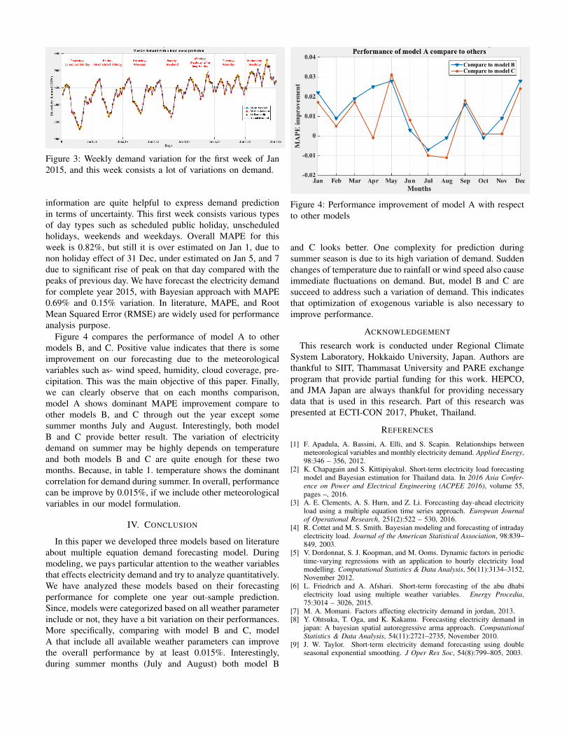
Figure 3: Weekly demand variation for the first week of Jan2015, and this week consists a lot of variations on demand.
information are quite helpful to express demand predictionin terms of uncertainty. This first week consists various typesof day types such as scheduled public holiday, unscheduledholidays, weekends and weekdays. Overall MAPE for thisweek is 0.82%, but still it is over estimated on Jan 1, due tonon holiday effect of 31 Dec, under estimated on Jan 5, and 7due to significant rise of peak on that day compared with thepeaks of previous day. We have forecast the electricity demandfor complete year 2015, with Bayesian approach with MAPE0.69% and 0.15% variation. In literature, MAPE, and RootMean Squared Error (RMSE) are widely used for performanceanalysis purpose.
Figure 4 compares the performance of model A to othermodels B, and C. Positive value indicates that there is someimprovement on our forecasting due to the meteorologicalvariables such as- wind speed, humidity, cloud coverage, pre-cipitation. This was the main objective of this paper. Finally,we can clearly observe that on each months comparison,model A shows dominant MAPE improvement compare toother models B, and C through out the year except somesummer months July and August. Interestingly, both modelB and C provide better result. The variation of electricitydemand on summer may be highly depends on temperatureand both models B and C are quite enough for these twomonths. Because, in table 1. temperature shows the dominantcorrelation for demand during summer. In overall, performancecan be improve by 0.015%, if we include other meteorologicalvariables in our model formulation.
IV. CONCLUSION
In this paper we developed three models based on literatureabout multiple equation demand forecasting model. Duringmodeling, we pays particular attention to the weather variablesthat effects electricity demand and try to analyze quantitatively.We have analyzed these models based on their forecastingperformance for complete one year out-sample prediction.Since, models were categorized based on all weather parameterinclude or not, they have a bit variation on their performances.More specifically, comparing with model B and C, modelA that include all available weather parameters can improvethe overall performance by at least 0.015%. Interestingly,during summer months (July and August) both model B
Figure 4: Performance improvement of model A with respectto other models
and C looks better. One complexity for prediction duringsummer season is due to its high variation of demand. Suddenchanges of temperature due to rainfall or wind speed also causeimmediate fluctuations on demand. But, model B and C aresucceed to address such a variation of demand. This indicatesthat optimization of exogenous variable is also necessary toimprove performance.
ACKNOWLEDGEMENT
This research work is conducted under Regional ClimateSystem Laboratory, Hokkaido University, Japan. Authors arethankful to SIIT, Thammasat University and PARE exchangeprogram that provide partial funding for this work. HEPCO,and JMA Japan are always thankful for providing necessarydata that is used in this research. Part of this research waspresented at ECTI-CON 2017, Phuket, Thailand.
REFERENCES
[1] F. Apadula, A. Bassini, A. Elli, and S. Scapin. Relationships betweenmeteorological variables and monthly electricity demand. Applied Energy,98:346 – 356, 2012.
[2] K. Chapagain and S. Kittipiyakul. Short-term electricity load forecastingmodel and Bayesian estimation for Thailand data. In 2016 Asia Confer-ence on Power and Electrical Engineering (ACPEE 2016), volume 55,pages –, 2016.
[3] A. E. Clements, A. S. Hurn, and Z. Li. Forecasting day-ahead electricityload using a multiple equation time series approach. European Journalof Operational Research, 251(2):522 – 530, 2016.
[4] R. Cottet and M. S. Smith. Bayesian modeling and forecasting of intradayelectricity load. Journal of the American Statistical Association, 98:839–849, 2003.
[5] V. Dordonnat, S. J. Koopman, and M. Ooms. Dynamic factors in periodictime-varying regressions with an application to hourly electricity loadmodelling. Computational Statistics & Data Analysis, 56(11):3134–3152,November 2012.
[6] L. Friedrich and A. Afshari. Short-term forecasting of the abu dhabielectricity load using multiple weather variables. Energy Procedia,75:3014 – 3026, 2015.
[7] M. A. Momani. Factors affecting electricity demand in jordan, 2013.[8] Y. Ohtsuka, T. Oga, and K. Kakamu. Forecasting electricity demand in
japan: A bayesian spatial autoregressive arma approach. ComputationalStatistics & Data Analysis, 54(11):2721–2735, November 2010.
[9] J. W. Taylor. Short-term electricity demand forecasting using doubleseasonal exponential smoothing. J Oper Res Soc, 54(8):799–805, 2003.
A Nepali Rule Based Stemmer and its performanceon different NLP applications
Pravesh KoiralaDepartment of Electronics and Computer Engineering
Institute Of Engineering, PulchowkKathmandu, Nepal
Aman ShakyaDepartment of Electronics and Computer Engineering
Institute Of Engineering, PulchowkKathmandu, Nepal
Abstract—Stemming is an integral part of NaturalLanguage Processing (NLP). It’s a preprocessing stepin almost every NLP application. Arguably, the mostimportant usage of stemming is in Information Re-trieval (IR). While there are lots of work done onstemming in languages like English, Nepali stemminghas only a few works. This study focuses on creating aRule Based stemmer for Nepali text. Specifically, it isan affix stripping system that identifies two differentclass of suffixes in Nepali grammar and strips themseparately. Only a single negativity prefix न is identifiedand stripped. This study focuses on a number of tech-niques like exception word identification, morphologi-cal normalization and word transformation to increasestemming performance. The stemmer is tested intrinsi-cally using Paice’s method and extrinsically on a basictf-idf based IR system and an elementary news topicclassifier using Multinomial Naive Bayes Classifier. Thedifference in performance of these systems with andwithout using the stemmer is analysed.
Index Terms—Nepali, Stemming, Over-Stemming,Under-Stemming, IR, tf-idf, Paice method, News TopicClassification
I. Introduction
Stemming refers to the reduction of a given word intoits stem which need not be the morphological root of theword. This is done to reduce the inflection of any particularword into a base form. For example: cats is the inflectedform of cat and stemming strips the plurality suffix -s fromcats to give cat.
Various NLP applications use stemming as a pre-processing step, for example: POS Tagging, MachineTranslation, Document Clustering etc but arguably themost important role of word stemming is in InformationRetrieval (IR). IR is an immensely common and importantapplication of Natural Language Processing. It essentiallyrefers to the retrieval of a particular document from acollection of documents.
There are two major problems while stemming: over-stemming and under-stemming. Over-stemming is whentwo separate inflected words are reduced to a same wordstem. This is a false-positive in IR, since it leads the IRsystem to fetch documents which might not contain thesearch query. Similarly, under-stemming is when two same
inflections of a word are not reduced to the same wordstem. This is false-negative. It leads to an IR system notfinding documents having a related word inflection.
Stemming is mostly done in three ways:• Rule Based Stemming• Statistical Stemming• Hybrid StemmingRule based stemming approaches generally refer to affix
stripping where a list of affixes are maintained and arestripped to stem a word. Similarly, statistical stemmingrefers to the usage of statistical models like HMMs andn-grams to stem a word. Hybrid stemming tends to com-bine aspects of both rule based stemming and statisticalstemming in hopes of improving stemming performance.The focus of this work is on rule based method.
II. Related WorksStemming is not an unfamiliar topic. Including the
renowned Porter stemmer, many works exist for stemmingwords in English. In Nepali, however, there are only afew works. Bal et al. wrote a morphological analyzer andstemmer for Nepali language [1]. Sitaula proposed a hybridnepali stemming algorithm which uses affix stripping inconjunction with a string similarity function and reportsa recall rate of 72.1% on 1200 words [2]. He has takeninto consideration a total of 150 suffixes and around 35prefixes. Paul et al. describes an affix removal stemmingalgorithm for Nepali text. Their work has a database of120 suffixes and 25 prefixes and a root lexicon of over1000 words and reports an overall accuracy of 90.48% [3].Shrestha et al. classifies suffixes into three categories andstem them according to different criterias [4]. They takeinto account 128 suffix rules and report an accuracy of88.78% on 5000 words.
There are also some works in languages which aremorphologically similar to Nepali. A hindi stemmer wasdevised by Ramanathan et al. [5] where they first usea transliteration scheme to transliterate Devanagari toEnglish. They have maintained a suffix list which is usedto strip the word by using the process of longest match.Upon testing the algorithm in 35977 words, 4.6% wordswere found to be under-stemmed while 13.8% were found

to be over-stemmed. An Urdu stemmer is also written byKansal et al. [6] which uses the rule based approach tostem Urdu words. They report 85.14% accuracy on morethan 20,000 words.
III. ChallengesThe fact that Nepali is an inherently complex language
makes it inaccessible to many analysis. Various deriva-tional and inflectional techniques exist in Nepali gram-mar which creates plethora of frequently used words ineveryday life. For instance, inflection alone is categorizedas being of ten types. These inflections can alter a word’sstructure based on gender, cardinality, respect, tense andits aspects. Moreover, inflections are also based on moods,voice, causality and negation [7]. This makes it non-trivial to devise a proper stemming algorithm for Nepalilanguage.
There is also a need to identify whether a linguisticentity attached at the end of the word is a suffix attachingitself to a base word or is actually a part of the worditself. For instance, in the word काल the entity ल is actuallythe part of the word itself whereas in the word कालल therightmost ल is a post-positional suffix. It is imperativeto accurately identify when and when not to strip agiven suffix because unnecessary stripping leads to over-stemming.
Another challenge in suffix stripping is the difference inwriting. For example, both of the word form सा कितक andसा कतीक are used interchangeably in informal writing. Un-less an assumption about strictness of the grammar rules,there is a need to include both of the suffixes ि◌क and ◌ीक.Not only that, several suffixes can be joined together asin उनीह को which contains two postpositions (ह and को)compounded together. To deal with these scenarios, thereis a need to repeatedly apply the stripping rules. However,this increases the chances of over-stemming.
IV. MethodologyA. Morphological Normalization
Among the vowels present in Nepali language, the vowelpairs <इ, ई> and <उ, ऊ> in both their dependant and independant forms are often confused while writing. Sameis the case with some of the consonant groups like <व,ब>. To make the stemmer more robust to these commongrammatical errors, a morphological normalization schemewas introduced where the often confused vowels and con-sonants are normalized into a single entity. Concretely, alloccurrence of the vowel ई are replaced with इ and so onwhile stemming the words. A more detailed normalizationscheme is outlined below.
B. Prefix StrippingThough there are many prefixes in Nepali, they have
not been stripped as a part of this work. This is mainlybecause the prefixes derive a new word from a root insteadof inflecting it. For instance, the words like उपकार, परकार,
TABLE IMorphological Normalization Rules
Vowel / Consonant Normalized Toइ ई◌ी ि◌ऊ उ◌ ◌व बश सष स◌ Nil (all occurances removed)
अिधकार, पिरकार etc all are words derived from the applica-tion of the prefixes उप, पर, अिध, पिर respectively to the sameroot कार. All of these words are actually totally unrelatedto each other so stripping prefixes would mean that theywould overstem.
An exception to this rule is the negativity prefix न. Itusually occurs before verbs and negates their sense. Forexample, the verb जान (to go) can be inflected as नजान (tonot go) by the application of this prefix. This work onlyconsiders this single prefix for stripping.
C. Suffix StrippingThe suffixes in Nepali language have been classified into
two classes in this work:• Type I suffix• Type II suffixType I suffixes mainly consists of post-positions and
other agglutinative suffixes. Some example of these suffixesare: मा, बाट, ल, लाई, ारा, लािग, िनि त etc. There are 85 type Isuffixes identified in this work.
Type II suffixes, on the other hand, primarily consist ofcase markers and other bound suffixes. Some of the suffixesalso occur in both free and bound form, for example ◌काand एका are linguistically the same but differ in that theformer has the dependant vowel ◌ and the second has theindependent vowel ए. Some examples of type II suffixesare: छ, न, छयौ, एको, इक etc. A total of 161 of these suffixeswere identified.
1) Stripping type I suffix: Stripping these suffixes is anon-trivial process. This can be attributed to two majorfacts:
To begin with, identification of these suffix is challeng-ing. As was discussed earlier, some of these suffixes occuras a part of word itself. For instance, the word नह is thename of a reputed Indian politician and not the suffix हattached to the root न. There are many more examples ofsuch exception words. Before stripping type I suffixes, anextensive exception word list has to be created and checkedagainst to prevent over-stemming. A total of 181 of theseexceptions words were identified by manually eyeballing acorpus derived from various online Nepali news sites. Thecorpus is described in section V-A.
Another challenge in stripping type I suffix is that thesesuffixes can be chained together i.e. the word उनीह लाई is
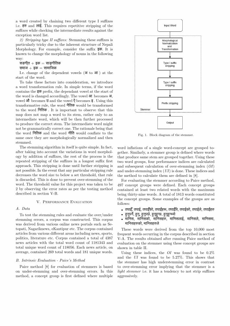
a word created by chaining two different type I suffixesi.e. ह and लाई. This requires repetitive stripping of thesuffixes while checking the intermediate results against theexception word list.
2) Stripping type II suffixes: Stemming these suffixes isparticularly tricky due to the inherent structure of NepaliMorphology. For example, consider the suffix इक. It isknown to change the morphology of nouns in the followingway:सङगीत + इक = सा गीितकसमाज + इक = सामािजकI.e. change of the dependent vowels (अ to आ ) at the
start of the word.To take these factors into consideration, we introduce
a word transformation rule. In simple terms, if the wordcontains the इक prefix, the dependant vowel at the start ofthe word is changed accordingly. The vowel आ becomes अ,vowel औ becomes उ and the vowel ए becomes इ . Using thistransformative rule, the word नितक would be transformedto the word िनितक . It is important to observe that thismap does not map a word to its stem, rather only to anintermediate word, which will be then further processedto produce the correct stem. The intermediate word mightnot be grammatically correct one. The rationale being thatthe word िनितक and the word नीित would conflate to thesame once they are morphologically normalized and thenstemmed.
The stemming algorithm in itself is quite simple. In fact,after taking into account the variations in word morphol-ogy by addition of suffixes, the rest of the process is therepeated stripping of the suffixes in a longest suffix firstapproach. This stripping is done until further stripping isnot possible. In the event that any particular stripping ruledecreases the word size to below a set threshold, that ruleis discarded. This is done to prevent over-stemming of theword. The threshold value for this project was taken to be2 by observing the error rates as per the testing methoddescribed in section V-B.
V. Performance EvaluationA. Data
To test the stemming rules and evaluate the over/understemming errors, a corpus was constructed. This corpuswas derived from various online news portals such as Se-topati, Nagariknews, eKantipur etc. The corpus containedarticles from various different areas including news, sports,politics, literature etc. Corpus contained a total of 4387news articles with the total word count of 1181343 andtotal unique word count of 118056. Each news article, onaverage, contained 269 total words and 181 unique words.
B. Intrinsic Evaluation - Paice’s MethodPaice method [8] for evaluation of stemmers is based
on under-stemming and over-stemming errors. In thismethod, a concept group is first defined where multiple
Fig. 1. Block diagram of the stemmer.
word inflations of a single word-concept are grouped to-gether. Similarly, a stemmer group is defined where wordsthat produce same stem are grouped together. Using thesetwo word groups, four performance indices are calculatedand subsequent calculation of over-stemming index (OI)and under-stemming index (UI) is done. These indices andthe method to calculate them are defined in [8].
For evaluating the stemmer according to Paice method,497 concept groups were defined. Each concept groupscontained at least two related words with the maximumbeing thirty-nine words. A total of 1813 words constitutedthe concept groups. Some examples of the groups are asfollows:
• तपाई, तपाई, तपाईको, तपाईह , तपाईल, तपाईको, तपाईल, तपाईह• हनपन, हन, हनपछ, हनह छ, हनह यो• मािनस, मािनसको, मािनसह , मािनसलाई, मािनसल, मािनसमा,मािनसह को, मािनसह ल
These words were derived from the top 10,000 mostfrequent words occurring in the corpus described in sectionV-A. The results obtained after running Paice method ofevaluation on the stemmer using these concept groups areshown in table II.
Using these indices, the OI was found to be 0.2%and the UI was found to be 5.27%. This shows thatthe stemmer has high understemming error in contrastto over-stemming error implying that the stemmer is alight stemmer i.e. it has a tendency to not strip suffixesaggressively.
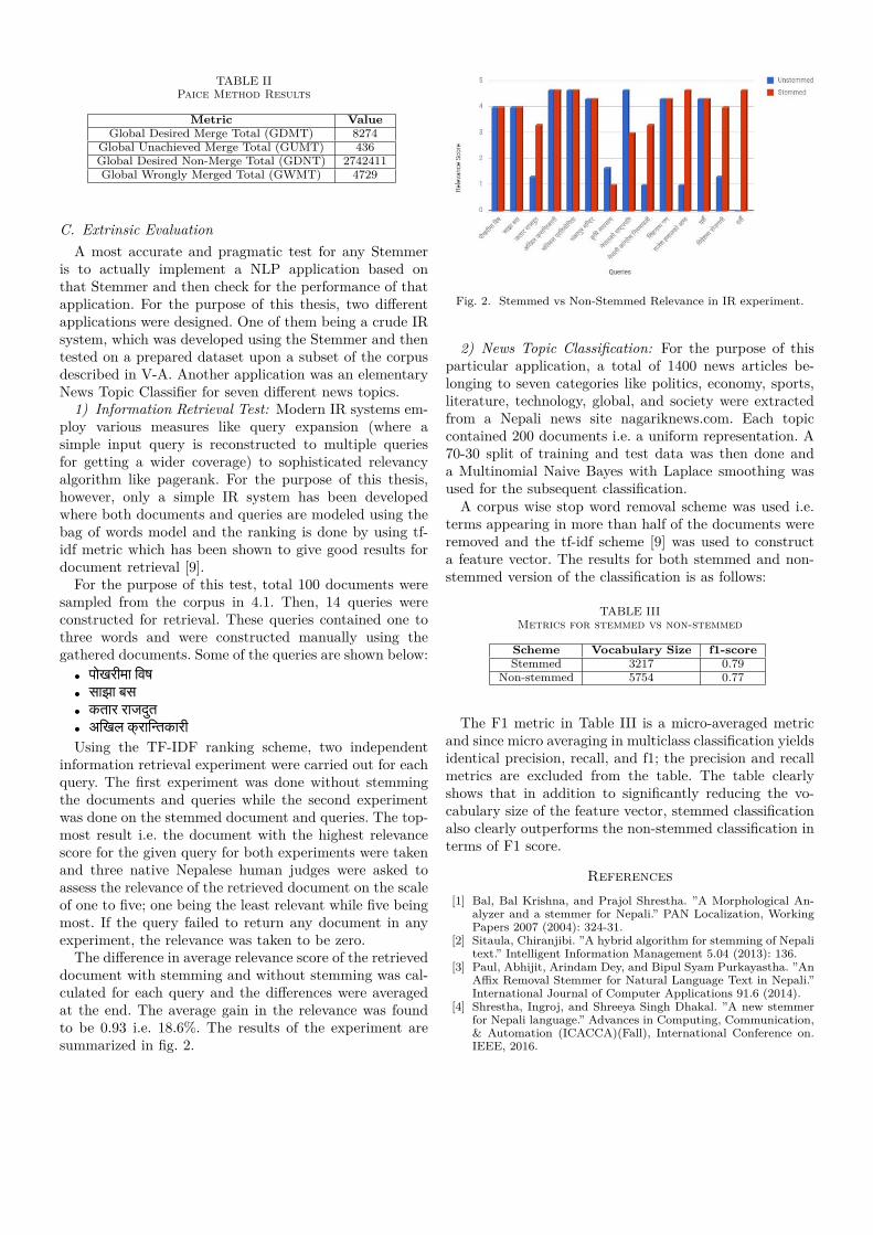
TABLE IIPaice Method Results
Metric ValueGlobal Desired Merge Total (GDMT) 8274
Global Unachieved Merge Total (GUMT) 436Global Desired Non-Merge Total (GDNT) 2742411Global Wrongly Merged Total (GWMT) 4729
C. Extrinsic EvaluationA most accurate and pragmatic test for any Stemmer
is to actually implement a NLP application based onthat Stemmer and then check for the performance of thatapplication. For the purpose of this thesis, two differentapplications were designed. One of them being a crude IRsystem, which was developed using the Stemmer and thentested on a prepared dataset upon a subset of the corpusdescribed in V-A. Another application was an elementaryNews Topic Classifier for seven different news topics.
1) Information Retrieval Test: Modern IR systems em-ploy various measures like query expansion (where asimple input query is reconstructed to multiple queriesfor getting a wider coverage) to sophisticated relevancyalgorithm like pagerank. For the purpose of this thesis,however, only a simple IR system has been developedwhere both documents and queries are modeled using thebag of words model and the ranking is done by using tf-idf metric which has been shown to give good results fordocument retrieval [9].
For the purpose of this test, total 100 documents weresampled from the corpus in 4.1. Then, 14 queries wereconstructed for retrieval. These queries contained one tothree words and were constructed manually using thegathered documents. Some of the queries are shown below:
• पोखरीमा िवष• साझा बस• कतार राजदत• अिखल कराि तकारीUsing the TF-IDF ranking scheme, two independent
information retrieval experiment were carried out for eachquery. The first experiment was done without stemmingthe documents and queries while the second experimentwas done on the stemmed document and queries. The top-most result i.e. the document with the highest relevancescore for the given query for both experiments were takenand three native Nepalese human judges were asked toassess the relevance of the retrieved document on the scaleof one to five; one being the least relevant while five beingmost. If the query failed to return any document in anyexperiment, the relevance was taken to be zero.
The difference in average relevance score of the retrieveddocument with stemming and without stemming was cal-culated for each query and the differences were averagedat the end. The average gain in the relevance was foundto be 0.93 i.e. 18.6%. The results of the experiment aresummarized in fig. 2.
Fig. 2. Stemmed vs Non-Stemmed Relevance in IR experiment.
2) News Topic Classification: For the purpose of thisparticular application, a total of 1400 news articles be-longing to seven categories like politics, economy, sports,literature, technology, global, and society were extractedfrom a Nepali news site nagariknews.com. Each topiccontained 200 documents i.e. a uniform representation. A70-30 split of training and test data was then done anda Multinomial Naive Bayes with Laplace smoothing wasused for the subsequent classification.
A corpus wise stop word removal scheme was used i.e.terms appearing in more than half of the documents wereremoved and the tf-idf scheme [9] was used to constructa feature vector. The results for both stemmed and non-stemmed version of the classification is as follows:
TABLE IIIMetrics for stemmed vs non-stemmed
Scheme Vocabulary Size f1-scoreStemmed 3217 0.79
Non-stemmed 5754 0.77
The F1 metric in Table III is a micro-averaged metricand since micro averaging in multiclass classification yieldsidentical precision, recall, and f1; the precision and recallmetrics are excluded from the table. The table clearlyshows that in addition to significantly reducing the vo-cabulary size of the feature vector, stemmed classificationalso clearly outperforms the non-stemmed classification interms of F1 score.
References[1] Bal, Bal Krishna, and Prajol Shrestha. ”A Morphological An-
alyzer and a stemmer for Nepali.” PAN Localization, WorkingPapers 2007 (2004): 324-31.
[2] Sitaula, Chiranjibi. ”A hybrid algorithm for stemming of Nepalitext.” Intelligent Information Management 5.04 (2013): 136.
[3] Paul, Abhijit, Arindam Dey, and Bipul Syam Purkayastha. ”AnAffix Removal Stemmer for Natural Language Text in Nepali.”International Journal of Computer Applications 91.6 (2014).
[4] Shrestha, Ingroj, and Shreeya Singh Dhakal. ”A new stemmerfor Nepali language.” Advances in Computing, Communication,& Automation (ICACCA)(Fall), International Conference on.IEEE, 2016.

[5] Ramanathan, Ananthakrishnan, and Durgesh D. Rao. ”Alightweight stemmer for Hindi.” the Proceedings of EACL. 2003.
[6] Lehal, Rohit Kansal Vishal Goyal GS. ”Rule Based Urdu Stem-mer.” 24th International Conference on Computational Linguis-tics. Vol. 267. 2012.
[7] Adhikari, H. R, Bhandar, B.P and Bhotahiti, SamasamayikNepali Vyakaran, Kathmandu, Third Edition 2062 B.S
[8] Paice, Chris D. ”An evaluation method for stemming algo-rithms.” Proceedings of the 17th annual international ACMSIGIR conference on Research and development in informationretrieval. Springer-Verlag New York, Inc., 1994.
[9] Ramos, Juan. ”Using tf-idf to determine word relevance in doc-ument queries.” Proceedings of the first instructional conferenceon machine learning. Vol. 242. 2003.

Agent Based Control of Multiple Power SourcesPurushotam Shrestha
Nepal College of Information TechnologyLalitpur, Nepal
Email: [email protected]
Abstract—The reliabilty of a power source can be increasedby using multiple types of sources with different attributes.Properties, such as environment friendliness of a solar powersystem, are preferable over attributes such as negative impactsand cost of diesel generating plants and utility grids. Whenusing such a multi-source system, a common challange is to usemaximum or all of the power produced by the most preferredsource. Conventional technique of simply connecting the outputsof the power sources cannot assure of the maximum utilization.The agent based approach developed in this paper maximizesthe utilization of the most preferred source and minimizes theuse of the least preferred one
Index Terms—Agent System, Bounded Knapsack Problem,Divide and Conquer Approach
I. INTRODUCTION
Telecom sites providing voice and data services need tooperate without interruption on 24-7 basis. Site down of evena small time period causes loss of important communicationand dissatisfaction on customer side and negative impact inthe revenue and good will of operators.
A point of failure of a telecom site is often the power supply.So, it is common to use more than one source of power in thesites. The goal of such a practice is to increase reliability androbustness of the power supply for un-interruptible operation.
The power systems employed in the telecom sites are het-erogeneous in nature varying in attributes such as purchase andinstallation price, operating cost, impact on the environmentetc. Some of the systems, because of the qualities, are morepreferable over others. And the trend is to use renewableenergy such as solar and wind power. But the intermittency ofthese sources make the output power unsteady and unreliable.So, these sources are be combined with existing power sourcessuch utility grid electricity and diesel generator. But the waythey are connected for the output, which is the combinedpower they supply, the desired source is not used at the desiredlevel.
II. LITERATURE REVIEW
The intermitency of renewable sources such as PV modulesand wind turbines do not allow users to depend upon them [1]and requires their integration with some steady sources suchas battery systems or the utility grid. While a steady powercan be derived from such a combination, no single sourceoutperforms others in all the metrics and the advantage of ahybrid system is evident as discussed in [2] . A hierarchicalorganization and operation of charging sources, conventionalbattery, fuel cell and capacitors as described in [2] has capacity
to store energy due to the battery as well as can quickly supplylarge currents due to the capacitor.
The goal of such a system may be one or all of thefollowing:
• Balance demand – supply during peak demand hours.• Cost balance by preferring use of a low cost energy
source.• Emphasize on use of greener technology.
[2] employs measurement systems that aid in control ofmultiple switches that interconnect energy sources and load.
[1] proposes a system architecture and control algorithmto minimize the use of grid electricity as far as possibleemphasizing use of energy stored in the battery or fromthe renewable sources to minimize grid costs at individualbuildings and eliminate demands during peak hours. Thealgorithm works in the context of Time Of Use (TOU) pricingbut without Net Metering. The cost reduction reported is 2.7X.The output power of different sources and the demand arepredicted using complex mathematical equations and fed tothe algorithm which outputs the amount of energy to use fromthe grid and the energy to charge or that can be dischargedfrom the battery.
Similarly, the use of neural network and fuzzy logic con-troller for adaptive scheme for energy management in stand-alone hybrid power system with photo voltaic (PV) modules,wind turbine (WT), Proton Exchange Membrane Fuel Cell(PEMFC) as energy sources and Lithium-ion battery as energystorage is discussed in [3]. The energy management systemuses artificial neural network to achieve Maximum PowerPoint (MPP) for different types of PV panels and the FLCto distribute energy among the hybrid system entities, managecharge and discharge current flow for performance optimiza-tion and to regulate the temperature of the PEMFC. Thecontroller is designed with hierarchical architecture and usesmathematical models to estimate the power being deliveredby the sources based upon the current values of the associatedparameters.
Microcontroller equipped with FPGA is used as a controllerfor a power management system in [4]. The power system con-sists of battery storage system, PEMFC, PV modules and a lowvoltage ac node and emphasis is given in controlling the SOCwhich is estimated using an algorithm that takes parameterssuch as battery current-time integration, open circuit voltage,electrolyte temperature, discharge rate and minimization ofstartup and shutdown of the PEMFC.
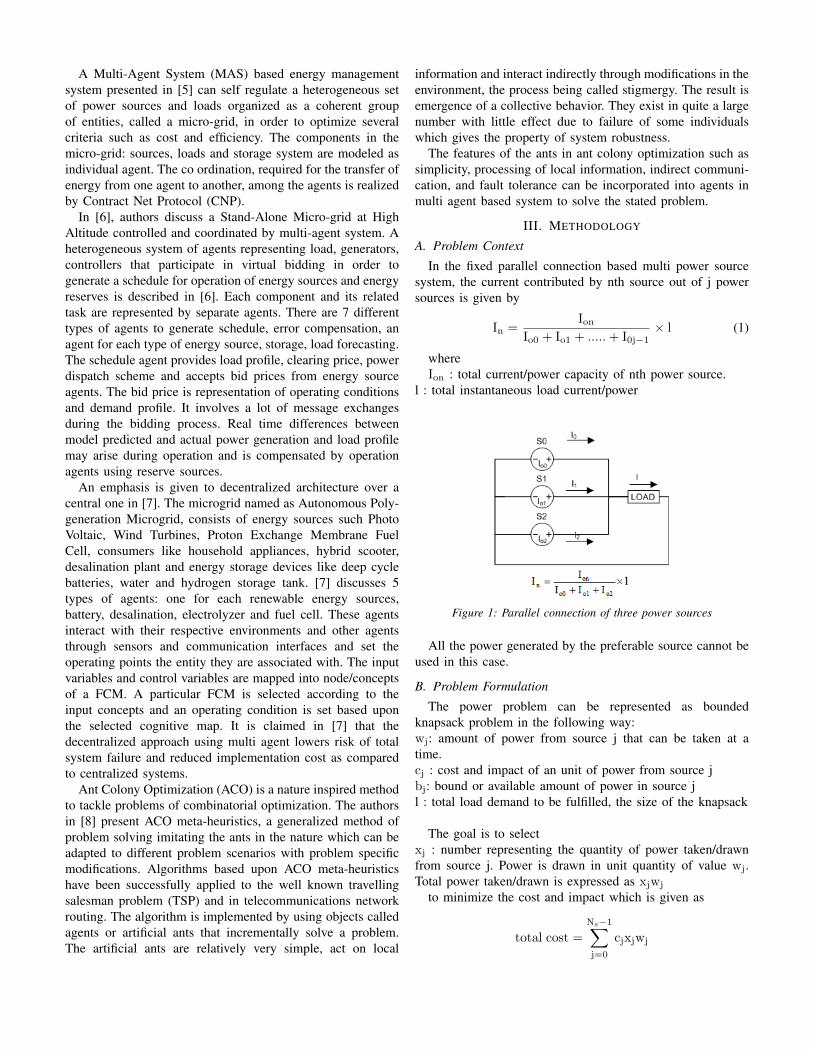
A Multi-Agent System (MAS) based energy managementsystem presented in [5] can self regulate a heterogeneous setof power sources and loads organized as a coherent groupof entities, called a micro-grid, in order to optimize severalcriteria such as cost and efficiency. The components in themicro-grid: sources, loads and storage system are modeled asindividual agent. The co ordination, required for the transfer ofenergy from one agent to another, among the agents is realizedby Contract Net Protocol (CNP).
In [6], authors discuss a Stand-Alone Micro-grid at HighAltitude controlled and coordinated by multi-agent system. Aheterogeneous system of agents representing load, generators,controllers that participate in virtual bidding in order togenerate a schedule for operation of energy sources and energyreserves is described in [6]. Each component and its relatedtask are represented by separate agents. There are 7 differenttypes of agents to generate schedule, error compensation, anagent for each type of energy source, storage, load forecasting.The schedule agent provides load profile, clearing price, powerdispatch scheme and accepts bid prices from energy sourceagents. The bid price is representation of operating conditionsand demand profile. It involves a lot of message exchangesduring the bidding process. Real time differences betweenmodel predicted and actual power generation and load profilemay arise during operation and is compensated by operationagents using reserve sources.
An emphasis is given to decentralized architecture over acentral one in [7]. The microgrid named as Autonomous Poly-generation Microgrid, consists of energy sources such PhotoVoltaic, Wind Turbines, Proton Exchange Membrane FuelCell, consumers like household appliances, hybrid scooter,desalination plant and energy storage devices like deep cyclebatteries, water and hydrogen storage tank. [7] discusses 5types of agents: one for each renewable energy sources,battery, desalination, electrolyzer and fuel cell. These agentsinteract with their respective environments and other agentsthrough sensors and communication interfaces and set theoperating points the entity they are associated with. The inputvariables and control variables are mapped into node/conceptsof a FCM. A particular FCM is selected according to theinput concepts and an operating condition is set based uponthe selected cognitive map. It is claimed in [7] that thedecentralized approach using multi agent lowers risk of totalsystem failure and reduced implementation cost as comparedto centralized systems.
Ant Colony Optimization (ACO) is a nature inspired methodto tackle problems of combinatorial optimization. The authorsin [8] present ACO meta-heuristics, a generalized method ofproblem solving imitating the ants in the nature which can beadapted to different problem scenarios with problem specificmodifications. Algorithms based upon ACO meta-heuristicshave been successfully applied to the well known travellingsalesman problem (TSP) and in telecommunications networkrouting. The algorithm is implemented by using objects calledagents or artificial ants that incrementally solve a problem.The artificial ants are relatively very simple, act on local
information and interact indirectly through modifications in theenvironment, the process being called stigmergy. The result isemergence of a collective behavior. They exist in quite a largenumber with little effect due to failure of some individualswhich gives the property of system robustness.
The features of the ants in ant colony optimization such assimplicity, processing of local information, indirect communi-cation, and fault tolerance can be incorporated into agents inmulti agent based system to solve the stated problem.
III. METHODOLOGY
A. Problem Context
In the fixed parallel connection based multi power sourcesystem, the current contributed by nth source out of j powersources is given by
In =Ion
Io0 + Io1 + .....+ I0j−1× l (1)
whereIon : total current/power capacity of nth power source.
l : total instantaneous load current/power
Figure 1: Parallel connection of three power sources
All the power generated by the preferable source cannot beused in this case.
B. Problem Formulation
The power problem can be represented as boundedknapsack problem in the following way:wj: amount of power from source j that can be taken at atime.cj : cost and impact of an unit of power from source jbj: bound or available amount of power in source jl : total load demand to be fulfilled, the size of the knapsack
The goal is to selectxj : number representing the quantity of power taken/drawnfrom source j. Power is drawn in unit quantity of value wj.Total power taken/drawn is expressed as xjwj
to minimize the cost and impact which is given as
total cost =
Ns−1∑j=0
cjxjwj

with the constraint
Ns−1∑j=0
wjxj ≤ l
where,0 ≤ xj ≤ bj , j ε [0,Ns] ,Ns is the number of types of powersources.The load demand should be exactly met, so the constraintshould be
Ns−1∑j=0
wjxj = l
C. Solution Approach
The approach of divide and conquer algorithm is used tosolve the problem. So the knapsack, l in our case, is dividedinto smaller knapsacks. Each smaller knapsack is filled withthe most preferable item as far as possible. Any smallerknapsack can be filled with power from any source. So, toreduce size mismatches in our solution, the size of all theportions are made equal, let the size be w.
w0 = w1 = w2 = wNs−1 = w
For simplicity, we consider a constant load. So l doesn’tchange. Since all the smaller portions of l are equal in sizeand each one is exactly fulfilled by using amount of powerequal to w, we can have
w NA = l
where NA is the number of smaller portions of l. Then we canhave relation for NA as
NA =l
w
The availability of power in preferable sources keeps chang-ing. For an arbitrary value of w, it is likely that the availablepower may not be in exact multiple of w. In order to usemost of the available power, the value of w must be chosencarefully. Two conditions may occur
1) after taking power of quantity (xj w) from source j, theremay be a surplus amount
2) the available power may be less than (xj w) and((xj − 1) w) may have to be taken leaving some surplusamount
If bj is the present available power, in the above describedcases, there is unused power which is given as
unused power = bj − xj w
The maximum unused power cannot be greater than w, becauseas soon as the unused power equals w, it will be used to fill asmaller knapsack, total power taken from that source will be
((xj + 1) w)
Figure 2: Multi-agent based solution concept
So, it can be inferred that the unused power can be reduced byreducing the value of w or increasing the number of smallerportions.
D. Algorithm Development
The first step is to determine the load, l, the system isrequired to fulfill and the acceptable error of unused power,w. And compute the number of smaller knapsacks NA.
Each smaller portion of l is be filled with power from themost preferable source, if that is not available, then the nextpreferred source and so on. An agent is employed to fill eachsmaller portion of l. Each agent can choose to connect to anyavailable power source. Figure 2 illustrates the concept of thesolution. The connection is now dynamic.
Initially, each agent is connected to the least preferablesource.
Because of the nature of the physical circuit, all the con-nected agents draw equal power from the source, the sum ofwhich is equal to the load demand l.
Each agent checks the available power sources in descend-ing order of preference starting at the most preferred one.When it makes a new connection, it compares the power it candraw from this new connection to the power it was drawingpreviously.
If the new value of power is greater than or equal to theprevious value, it keeps the new connection.
Else, if the new value is smaller than the previous value,it leaves the connection and goes on to try other remainingsources.
If no source can satisfy the condition, the least preferablesource will, because it is designed with enough capacity thatcan suffice the maximum load.
At any time, the load is fulfilled by combining the powereach agent is drawing from the sources.
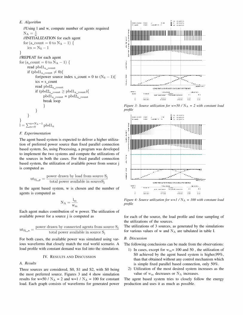
E. Algorithm
//Using l and w, compute number of agents requiredNA = l
w//INITIALIZATION for each agentfor (a count = 0 to NA − 1) {ics = NS − 1
}//REPEAT for each agentfor (a count = 0 to NA − 1) {
read pbd1a count
if (pbd1a count 6= 0){for(power source index s count = 0 to (NS − 1){ics = s countread pbd2a count
if (pbd2a count ≥ pbd1a count){pbd1a count = pbd2a count
break loop}
}}
}l =
∑n=NA−1n=0 pbd1n
F. Experimentation
The agent based system is expected to deliver a higher utiliza-tion of preferred power source than fixed parallel connectionbased system. So, using Processing, a program was developedto implement the two systems and compute the utilizations ofthe sources in both the cases. For fixed parallel connectionbased system, the utilization of available power from source jis computed as
utSj p =power drawn by load from source Sjtotal power available in sourceSj
In the agent based system, w is chosen and the number ofagents is computed as
NA =lmwm
Each agent makes contribution of w power. The utilization ofavailable power for a source j is computed as
utSj a =power drawn by connected agents from source Sj
total power available in source Sj
For both cases, the available power was simulated using var-ious waveforms that closely match the real world scenario. Aload profile with constant demand was fed into the simulation.
IV. RESULTS AND DISCUSSION
A. Results
Three sources are considered, S0, S1 and S2, with S0 beingthe most preferred source. Figures 3 and 4 show simulationresults for w=50 / NA = 2 and w=1 / NA = 100 for constantload. Each graph consists of waveforms for generated power
Figure 3: Source utilization for w=50 / NA = 2 with constant loadprofile
Figure 4: Source utilization for w=1 / NA = 100 with constant loadprofile
for each of the source, the load profile and time sampling ofthe utilizations of the sources.The utilizations of 3 sources, as generated by the simulationsfor various values of w and NA are tabulated in table I.
B. Discussion
The following conclusions can be made from the observations:1) In cases, except for wm= 100 and 50 , the utilization of
S0 achieved by the agent based system is higher,99%,than that obtained without any control mechanism whichis simple fixed parallel based connection, only 50%.
2) Utilization of the most desired system increases as thevalue of wm decreases or NA increases.
The agent based system tries to closely follow the energyproduction and uses it as much as possible.
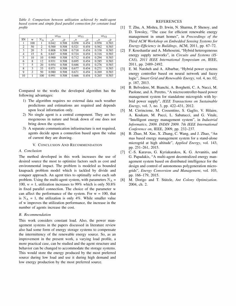
Table I: Comparison between utilization achieved by multi-agentbased system and simple fixed parallel connection for constant loadprofile
utS0 utS1 utS2SN w NA a p a p a p1 100 1 0.042 0.508 0.058 0.454 0.958 0.5832 50 2 0.500 0.508 0.521 0.454 0.562 0.5833 20 5 0.808 0.508 0.718 0.454 0.338 0.5834 15 6 0.847 0.508 0.724 0.454 0.316 0.5835 10 10 0.900 0.508 0.712 0.454 0.294 0.5836 8 12 0.931 0.508 0.695 0.454 0.285 0.5837 5 20 0.954 0.508 0.686 0.454 0.276 0.5838 3 33 0.971 0.508 0.677 0.454 0.271 0.5839 2 50 0.980 0.508 0.671 0.454 0.269 0.583
10 1 100 0.991 0.508 0.666 0.454 0.265 0.583
Compared to the works the developed algorithm has thefollowing advantages:
1) The algorithm requires no external data such weatherpredictions and estimations are required and dependsupon local information only.
2) No single agent is a central component. They are ho-mogeneous in nature and break down of one does notbring down the system.
3) A separate communication infrastructure is not required,agents decide upon a connection based upon the valueof current they are drawing.
V. CONCLUSION AND RECOMMENDATION
A. Conclusion
The method developed in this work increases the use ofdesired source the most to optimize factors such as cost andenvironmental impact. The problem is modeled as boundedknapsack problem model which is tackled by divide andconquer approach. An agent tries to optimally solve each subproblem. Using the multi-agent system, with parameters NA =100, w = 1, utilization increases to 99% which is only 50.8%in fixed parallel connection. The choice of the parameter wcan affect the performance of the system. For w = 100, thatis NA = 1, the utilization is only 4%. While smaller valueof w improves the utilization performance, the increase in thenumber of agents increase the cost.
B. Recommendation
This work considers constant load. Also, the power man-agement systems in the papers discussed in literature reviewalso had some form of energy storage systems to compensatethe intermittency of the renewable energy source. So, as animprovement in the present work, a varying load profile, amore practical case, can be studied and the agent structure andbehavior can be changed to accommodate the storage systems.This would store the energy produced by the most preferredsource during low load and use it during high demand andlow energy production by the most preferred source.
REFERENCES
[1] T. Zhu, A. Mishra, D. Irwin, N. Sharma, P. Shenoy, andD. Towsley, “The case for efficient renewable energymanagement in smart homes”, in Proceedings of theThird ACM Workshop on Embedded Sensing Systems forEnergy-Efficiency in Buildings, ACM, 2011, pp. 67–72.
[2] F. Koushanfar and A. Mirhoseini, “Hybrid heterogeneousenergy supply networks”, in Circuits and Systems (IS-CAS), 2011 IEEE International Symposium on, IEEE,2011, pp. 2489–2492.
[3] E. M. Natsheh and A. Albarbar, “Hybrid power systemsenergy controller based on neural network and fuzzylogic”, Smart Grid and Renewable Energy, vol. 4, no. 02,p. 187, 2013.
[4] B. Belvedere, M. Bianchi, A. Borghetti, C. A. Nucci, M.Paolone, and A. Peretto, “A microcontroller-based powermanagement system for standalone microgrids with hy-brid power supply”, IEEE Transactions on SustainableEnergy, vol. 3, no. 3, pp. 422–431, 2012.
[5] M. Cirrincione, M. Cossentino, S. Gaglio, V. Hilaire,A. Koukam, M. Pucci, L. Sabatucci, and G. Vitale,“Intelligent energy management system”, in IndustrialInformatics, 2009. INDIN 2009. 7th IEEE InternationalConference on, IEEE, 2009, pp. 232–237.
[6] B. Zhao, M. Xue, X. Zhang, C. Wang, and J. Zhao, “Anmas based energy management system for a stand-alonemicrogrid at high altitude”, Applied Energy, vol. 143,pp. 251–261, 2015.
[7] C.-S. Karavas, G. Kyriakarakos, K. G. Arvanitis, andG. Papadakis, “A multi-agent decentralized energy man-agement system based on distributed intelligence for thedesign and control of autonomous polygeneration micro-grids”, Energy Conversion and Management, vol. 103,pp. 166–179, 2015.
[8] M. Dorigo and T. Stutzle, Ant Colony Optimization.2004, ch. 2.
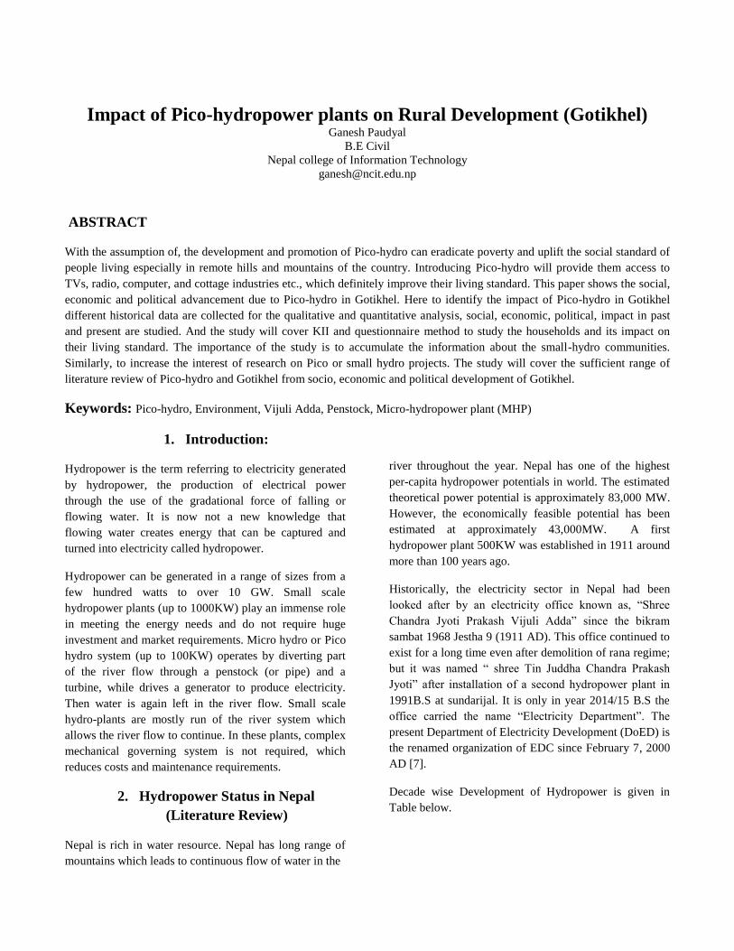
Impact of Pico-hydropower plants on Rural Development (Gotikhel) Ganesh Paudyal
B.E Civil
Nepal college of Information Technology
ABSTRACT
With the assumption of, the development and promotion of Pico-hydro can eradicate poverty and uplift the social standard of
people living especially in remote hills and mountains of the country. Introducing Pico-hydro will provide them access to
TVs, radio, computer, and cottage industries etc., which definitely improve their living standard. This paper shows the social,
economic and political advancement due to Pico-hydro in Gotikhel. Here to identify the impact of Pico-hydro in Gotikhel
different historical data are collected for the qualitative and quantitative analysis, social, economic, political, impact in past
and present are studied. And the study will cover KII and questionnaire method to study the households and its impact on
their living standard. The importance of the study is to accumulate the information about the small-hydro communities.
Similarly, to increase the interest of research on Pico or small hydro projects. The study will cover the sufficient range of
literature review of Pico-hydro and Gotikhel from socio, economic and political development of Gotikhel.
Keywords: Pico-hydro, Environment, Vijuli Adda, Penstock, Micro-hydropower plant (MHP)
1. Introduction:
Hydropower is the term referring to electricity generated
by hydropower, the production of electrical power
through the use of the gradational force of falling or
flowing water. It is now not a new knowledge that
flowing water creates energy that can be captured and
turned into electricity called hydropower.
Hydropower can be generated in a range of sizes from a
few hundred watts to over 10 GW. Small scale
hydropower plants (up to 1000KW) play an immense role
in meeting the energy needs and do not require huge
investment and market requirements. Micro hydro or Pico
hydro system (up to 100KW) operates by diverting part
of the river flow through a penstock (or pipe) and a
turbine, while drives a generator to produce electricity.
Then water is again left in the river flow. Small scale
hydro-plants are mostly run of the river system which
allows the river flow to continue. In these plants, complex
mechanical governing system is not required, which
reduces costs and maintenance requirements.
2. Hydropower Status in Nepal
(Literature Review)
Nepal is rich in water resource. Nepal has long range of
mountains which leads to continuous flow of water in the
river throughout the year. Nepal has one of the highest
per-capita hydropower potentials in world. The estimated
theoretical power potential is approximately 83,000 MW.
However, the economically feasible potential has been
estimated at approximately 43,000MW. A first
hydropower plant 500KW was established in 1911 around
more than 100 years ago.
Historically, the electricity sector in Nepal had been
looked after by an electricity office known as, “Shree
Chandra Jyoti Prakash Vijuli Adda” since the bikram
sambat 1968 Jestha 9 (1911 AD). This office continued to
exist for a long time even after demolition of rana regime;
but it was named “ shree Tin Juddha Chandra Prakash
Jyoti” after installation of a second hydropower plant in
1991B.S at sundarijal. It is only in year 2014/15 B.S the
office carried the name “Electricity Department”. The
present Department of Electricity Development (DoED) is
the renamed organization of EDC since February 7, 2000
AD [7].
Decade wise Development of Hydropower is given in
Table below.
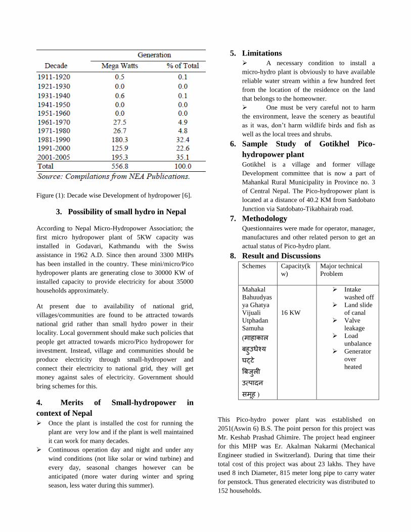
Figure (1): Decade wise Development of hydropower [6].
3. Possibility of small hydro in Nepal
According to Nepal Micro-Hydropower Association; the
first micro hydropower plant of 5KW capacity was
installed in Godavari, Kathmandu with the Swiss
assistance in 1962 A.D. Since then around 3300 MHPs
has been installed in the country. These mini/micro/Pico
hydropower plants are generating close to 30000 KW of
installed capacity to provide electricity for about 35000
households approximately.
At present due to availability of national grid,
villages/communities are found to be attracted towards
national grid rather than small hydro power in their
locality. Local government should make such policies that
people get attracted towards micro/Pico hydropower for
investment. Instead, village and communities should be
produce electricity through small-hydropower and
connect their electricity to national grid, they will get
money against sales of electricity. Government should
bring schemes for this.
4. Merits of Small-hydropower in
context of Nepal
➢ Once the plant is installed the cost for running the
plant are very low and if the plant is well maintained
it can work for many decades.
➢ Continuous operation day and night and under any
wind conditions (not like solar or wind turbine) and
every day, seasonal changes however can be
anticipated (more water during winter and spring
season, less water during this summer).
5. Limitations
➢ A necessary condition to install a
micro-hydro plant is obviously to have available
reliable water stream within a few hundred feet
from the location of the residence on the land
that belongs to the homeowner.
➢ One must be very careful not to harm
the environment, leave the scenery as beautiful
as it was, don’t harm wildlife birds and fish as
well as the local trees and shrubs.
6. Sample Study of Gotikhel Pico-
hydropower plant
Gotikhel is a village and former village
Development committee that is now a part of
Mahankal Rural Municipality in Province no. 3
of Central Nepal. The Pico-hydropower plant is
located at a distance of 40.2 KM from Satdobato
Junction via Satdobato-Tikabhairab road.
7. Methodology
Questionnaires were made for operator, manager,
manufactures and other related person to get an
actual status of Pico-hydro plant.
8. Result and Discussions
Schemes Capacity(k
w)
Major technical
Problem
Mahakal
Bahuudyas
ya Ghatya
Vijuali
Utphadan
Samuha
(माहाकाल
बहउधशय
घटट
बबजली उतपादन
समह )
16 KW
➢ Intake
washed off
➢ Land slide
of canal
➢ Valve
leakage
➢ Load
unbalance
➢ Generator
over
heated
This Pico-hydro power plant was established on
2051(Aswin 6) B.S. The point person for this project was
Mr. Keshab Prashad Ghimire. The project head engineer
for this MHP was Er. Akalman Nakarmi (Mechanical
Engineer studied in Switzerland). During that time their
total cost of this project was about 23 lakhs. They have
used 8 inch Diameter, 815 meter long pipe to carry water
for penstock. Thus generated electricity was distributed to
152 households.

Story is different after the National grids have been
reached to village. The entire household sifted towards
the national grid in 2066 B.S. As grid power is continuous
and free from technical issues with public. As there was
maintenance and load unbalance problem in Pico-
hydropower plant. Now this Pico-hydro is run by Mr.
Keshab Ghimire himself and has started a small Rice mill
utilizing the Pico electric power. It has given employment
to 1 skill manpower.
However, this Pico-hydro has brought huge socio-
economic and political impact to the village. This hydro
connected to the village with outer world and raised lots
of hope to the people living there.
Here in the below, before and after impact of Pico-hydro
is shown along with socio-economic and political
dimensions.
Dime
nsion
s
Before After Remarks
Social
Households
used to use
kerosene
and fire
woods.
Lack of
source of
information.
Less
working
hours.
Household
s got
connected
with
electric
energy.
Access to
informatio
n through
Radio,
television
etc.
Increase in
working
hours.
Less
use of
kerose
ne
and
fire
wood
s after
Pico
hydro
power
.
Societ
y
beco
mes
more
aware
.
Peopl
e got
involv
ed
early
morni
ng to
late
eveni
ng.
Econ
omic
Orthodox
agriculture.
Dependent
on
household
activities.
Equipped
with
modern
agricultura
l
techniques
.
They used
to feed
vegetables
to cattle.
Pico-hydro
provided
instant job
for 4
people.
Impac
t of
agricu
ltural
progra
ms of
radio,
televi
sion
etc.
Starte
d
sellin
g
vegeta
bles
to
near
marke
t.
Pico
hydro
create
d job
oppor
tunity
to 4
peopl
e.
Politi
cal
Literacy rate
was below
Were just
the voters
Literacy
rate
increases.
Now their
representat
ive is a
ward
chairperso
n (Ganga
ram
Timilsina)
Awar
eness
towar
ds
educat
ion.
Forwa
rd in
politic
al
leader
ship.
Discussion: Sample study of Gotikhel shows that Pico-
hydro had a significant impact on the development of
Gotikhel. It is found that consumption of firewood had
decrease. After that the children are found not to be
engaged in wood collection for firewood. Similarly it was
found that student have got more time to study during
night. People in the society now have access to outer
world through Information Communication and
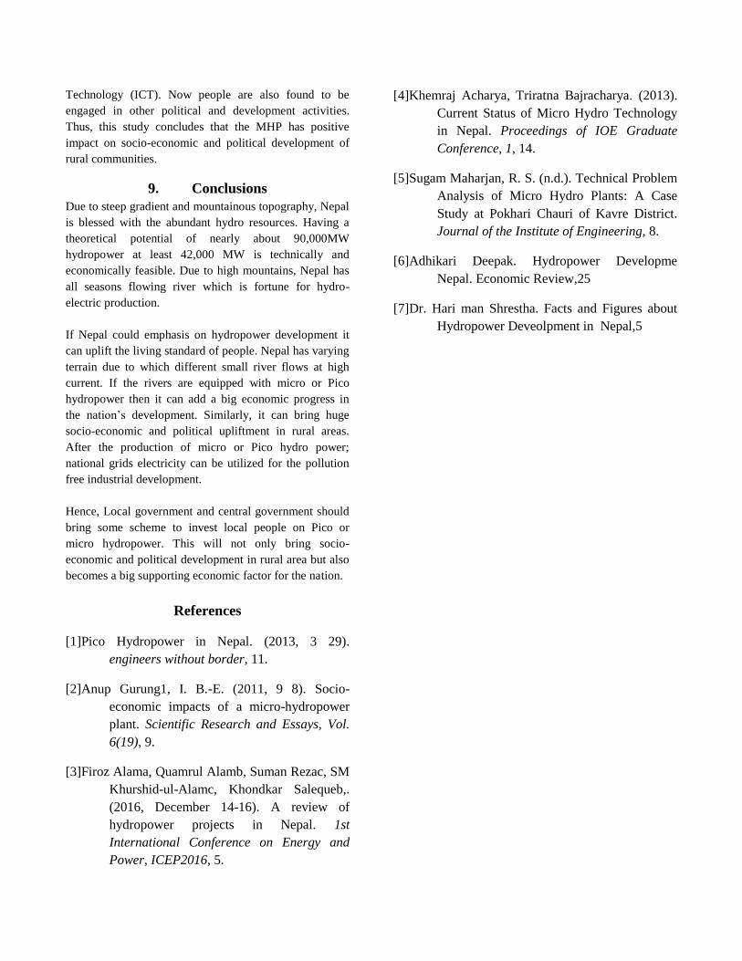
Technology (ICT). Now people are also found to be
engaged in other political and development activities.
Thus, this study concludes that the MHP has positive
impact on socio-economic and political development of
rural communities.
9. Conclusions
Due to steep gradient and mountainous topography, Nepal
is blessed with the abundant hydro resources. Having a
theoretical potential of nearly about 90,000MW
hydropower at least 42,000 MW is technically and
economically feasible. Due to high mountains, Nepal has
all seasons flowing river which is fortune for hydro-
electric production.
If Nepal could emphasis on hydropower development it
can uplift the living standard of people. Nepal has varying
terrain due to which different small river flows at high
current. If the rivers are equipped with micro or Pico
hydropower then it can add a big economic progress in
the nation’s development. Similarly, it can bring huge
socio-economic and political upliftment in rural areas.
After the production of micro or Pico hydro power;
national grids electricity can be utilized for the pollution
free industrial development.
Hence, Local government and central government should
bring some scheme to invest local people on Pico or
micro hydropower. This will not only bring socio-
economic and political development in rural area but also
becomes a big supporting economic factor for the nation.
References
[1]Pico Hydropower in Nepal. (2013, 3 29).
engineers without border, 11.
[2]Anup Gurung1, I. B.-E. (2011, 9 8). Socio-
economic impacts of a micro-hydropower
plant. Scientific Research and Essays, Vol.
6(19), 9.
[3]Firoz Alama, Quamrul Alamb, Suman Rezac, SM
Khurshid-ul-Alamc, Khondkar Salequeb,.
(2016, December 14-16). A review of
hydropower projects in Nepal. 1st
International Conference on Energy and
Power, ICEP2016, 5.
[4]Khemraj Acharya, Triratna Bajracharya. (2013).
Current Status of Micro Hydro Technology
in Nepal. Proceedings of IOE Graduate
Conference, 1, 14.
[5]Sugam Maharjan, R. S. (n.d.). Technical Problem
Analysis of Micro Hydro Plants: A Case
Study at Pokhari Chauri of Kavre District.
Journal of the Institute of Engineering, 8.
[6]Adhikari Deepak. Hydropower Developme
Nepal. Economic Review,25
[7]Dr. Hari man Shrestha. Facts and Figures about
Hydropower Deveolpment in Nepal,5

An Analysis of Heart Disease Prediction using Different Data
Mining Techniques
N. Sharmila, S. Aashish Kumar, G. Manoj
Department of Computer Science and Engineering
Nepal College of Information Technology
Balkumari, Lalitpur, Nepal
[email protected], [email protected], [email protected]
Abstract - Data mining is one of the important fields
of research whose significant goal is to find a useful
pattern of data from large data sets. After analysing,
the discovered pattern can be used to make decisions
on a different field like healthcare industry. With the
increase in worldwide population and evolution of
different new diseases along with old diseases,
healthcare industry produces numerous amounts of
data on a regular basis. Heart disease is a word that
collectively represents different medical disorder
related to the heart and directly affects the heart. On
treatment or during research, the healthcare industry
collects numbers of data related to heart disease
which contains hidden information that can be
important in making decisions. With data mining
techniques it is possible to analyse those data from
different aspects to create a relationship among them.
This paper works on the utilization of various decision
tree algorithms of data mining in order to predict
heart diseases.
Keywords: Heart Disease, Naïve Bayes, Neural
Networks, Decision Tree
I. INTRODUCTION
Data mining is one of the most crucial, powerful and
motivating fields of research which involves extraction of
helpful, meaningful and interesting information from a
collection of data. It can also be introduced as the process
of knowledge discovery from already existing
information. The main concern behind the concept of data
mining is finding hidden relationships among the data
present in different area like business, scientific and
medical to allow experts of those areas to make
predictions for future use. Hence, the main goal of data
mining is Extraction and Predictions. Data mining
involves different techniques like classification,
clustering, and association. Regarding medical research,
it is one of very appropriate approach as it assists the
medical researcher to predict and detect diseases by
gaining knowledge from patient's database.
II. HEART DISEASE
The heart is one of the most important parts of our body.
Improper operation of the heart will affect the other body
parts of human such as brain, kidney etc. It supports life
by its function of supplying blood throughout the body.
Without proper working of the heart it’s impossible for
any creature to live its life.
The term, Heart disease describes the disorders or
malfunctioning of the heart. There are different forms of
heart disease like heart attack, heart failure,
Cardiomyopathies and so on. Despite the genetic
problems, there are many factors which arise these types
of disease like unhealthy lifestyle, lack of exercise, high
cholesterol, high sugar level, and stress.
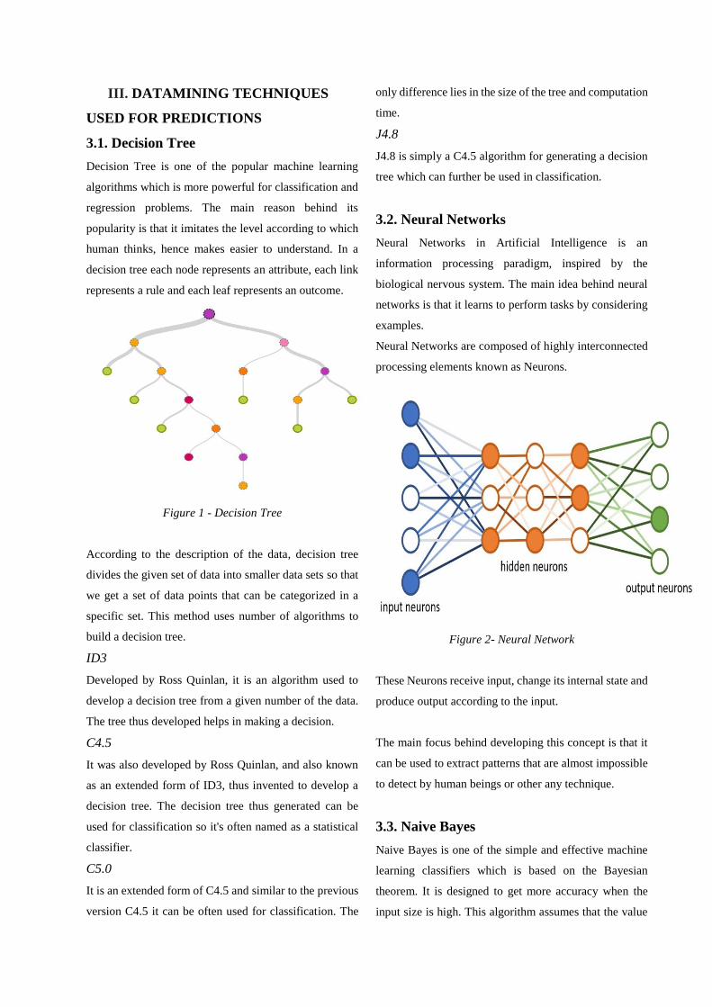
III. DATAMINING TECHNIQUES
USED FOR PREDICTIONS
3.1. Decision Tree
Decision Tree is one of the popular machine learning
algorithms which is more powerful for classification and
regression problems. The main reason behind its
popularity is that it imitates the level according to which
human thinks, hence makes easier to understand. In a
decision tree each node represents an attribute, each link
represents a rule and each leaf represents an outcome.
Figure 1 - Decision Tree
According to the description of the data, decision tree
divides the given set of data into smaller data sets so that
we get a set of data points that can be categorized in a
specific set. This method uses number of algorithms to
build a decision tree.
ID3
Developed by Ross Quinlan, it is an algorithm used to
develop a decision tree from a given number of the data.
The tree thus developed helps in making a decision.
C4.5
It was also developed by Ross Quinlan, and also known
as an extended form of ID3, thus invented to develop a
decision tree. The decision tree thus generated can be
used for classification so it's often named as a statistical
classifier.
C5.0
It is an extended form of C4.5 and similar to the previous
version C4.5 it can be often used for classification. The
only difference lies in the size of the tree and computation
time.
J4.8
J4.8 is simply a C4.5 algorithm for generating a decision
tree which can further be used in classification.
3.2. Neural Networks
Neural Networks in Artificial Intelligence is an
information processing paradigm, inspired by the
biological nervous system. The main idea behind neural
networks is that it learns to perform tasks by considering
examples.
Neural Networks are composed of highly interconnected
processing elements known as Neurons.
Figure 2- Neural Network
These Neurons receive input, change its internal state and
produce output according to the input.
The main focus behind developing this concept is that it
can be used to extract patterns that are almost impossible
to detect by human beings or other any technique.
3.3. Naive Bayes
Naive Bayes is one of the simple and effective machine
learning classifiers which is based on the Bayesian
theorem. It is designed to get more accuracy when the
input size is high. This algorithm assumes that the value

of a particular feature doesn't depends of the value of any
other feature on the given set of data.
Let's consider a hypothesis H and let E be the evidence.
Now, according to the Bayes’ Theorem the probability of
H before getting E and the probability of H after getting
E is:
P(H/E) = P(E/H) P(H)
P(E)
IV. LITERATURE REVIEW
Numerous researches have been done and numbers of
algorithms were implemented in heart disease prediction
by a number of authors. Different data mining algorithms
were carried out on different data consisting of a different
number of attributes. As per their work, they got their
result but the accuracy on the prediction varies according
to the attributes taken and method used. In this paper, we
aim to analyse different data mining technique which has
been used to predict heart disease.
P. Atul Kumar [1] has proposed the prediction using 14
attributes. the training data set and test data taken by him
was 200 and 103 respectively. Tangara [8], used 3000
data instances with 14 attributes too. the data set was
divided into two parts as 70% and 30% as training data
and test data which was implemented [9] on these
algorithms and the result of these algorithm were
recorded.
K. Thenmozhi [3] proposed a prediction model for the
Heart disease using 15 attributes [5]. The attributes taken
in this model were age, sex, chest pain, resting blood
pressure, serum cholesterol, resting electrographic,
Fasting blood sugar, Maximum heart rate achieved,
Exercise induced again, ST depression induced by
exercise relative to, Slope of the peak exercise, Number
of major vessels coloured by fluoroscopy, Defect type,
obesity, and smoking. For the prediction of the heart
disease, Naive Bayes, Decision Tree and Neural
Networks techniques were used in this model.
M. Lavanya [4] proposed a prediction model for heart
disease in the year 2016. The data were taken from South
Africa. They proposed the model with 11 attributes. The
attributes taken were a patient identification number,
gender, cardiogram, age, chest pain, blood pressure level,
heart rate, cholesterol, smoking, alcohol consumption,
and blood sugar level. J48 decision tree, Naive Bayes and
Artificial Neural Networks technique were used in the
prediction technique.
B. Nidhi [7] has used 13 attributes and then reduced the
attributes into 6 and implemented the different algorithms
for their result.
The different results have been summarized in the table
below.
Techniques
Used
Accuracy (%)
Different number of Attributes
6 11 13 14 15
Decision
Tree
96.6 91.85 94.44 52.33 90.74
Naive
Bayes
99.2 85.92 96.66 52 99.62
ANN 85.53 99.25 99.23 45.67 100
Table 1: Comparison of accuracy with Attributes
V. CONCLUSION
On analysing the data, we got from different papers we
can see that Neural Networks techniques provide high
accuracy on comparison with Decision tree and Naive
Bayes. The number and type of attributes taken were
different so we can say that accuracy depends on what
and how many attributes were taken.
On comparing these facts. The attributes taken are more
common and some differs. Those which differs may have
affected the efficiency. The papers have not clearly stated
the effect of single attribute to classifier result so the
difference on these attributes may have changed the
results from one another.

Similarly, the amount of data taken to train the system
and the amount of data used for testing makes the
difference in the accuracy and results of predicting the
heart disease.
Hence, we can conclude that for the classification, the
selection of proper attributes is the major concern. There
may be many other attributes like family history, job class
etc. which can directly effect the occurrence of heart
diseases. So, by this study we can suggest that effect of
single attribute and other highly affecting attributes can
be involved in the classification for the better results.
Similarly, we can also say that the number of data sets
taken to train the system will always vary the accuracy.
The more the training data, the more will be the accuracy
in classification.
Thus, by this study, we can conclude that, Artificial
Neural Network is best in classification technique with
large data set for training the system and with appropriate
set of attributes.
REFRENCES
[1] P. Atul Kumar, P. Prabhat, K.L. Jaiswal and S. Ashok
Kumar, “A Novel Frequent Feature Prediction Model for
Heart Disease Diagnosis”, International Journal of
Software & Hardware Research in Engineering, Vol. 1,
Issue. 1, September 2013.
[2] Tina R. Patil, S.S. Sherekar, “Performance Analysis
of Naïve Bayes and J48 Classification algorithm for Data
Classification”, International Journal of Computer
Science and Applications, Vol. 6, No. 2, Apr 2013.
[3] K. Thenmozhi, P. Deepika, "Heart Disease Prediction
Using Classification with Different Decision Tree
Techniques", International Journal of Engineering
Research and General Science Volume 2, Issue 6,
October-November, 2014.
[4] M. Lavanya, P.M. Gomathi, "Prediction of Heart
Disease using Classification Algorithms", International
Journal of Advanced Research in Computer Engineering
& Technology (IJARCET) Volume 5, Issue 7, July 2016.
[5] Chaitrali S. Dangare and Sulabha S. Apte, “Improved
Study of Heart Disease Prediction Using Data Mining
Classification Techniques”, International Journal of
Computer Applications, Vol. 47, No. 10, pp. 0975-888,
2012.
[6] N. Aditya Sundar, P. Pushpa Latha, M. Rama
Chandra, "Performance analysis of classification data
mining techniques over heart diseases data base" ,
international journal of engineering science and advanced
technology, 2012.
[7] B. Nidhi, J. Kiran, "An Analysis of Heart Diseases
Prediction by Using different datamining techniques",
international journal of engineering science and advanced
technology, ISSN:2278-0181, 2012.
[8] http://eric.univlyon2.fr/~ricco/tanagra/
[9] Asha Rajkumar, G. Sophia Reena, Diagnosis of Heart
Diseases Using Datamining Algorithm, Global Journal of
Computer Science and Technology, vol. 10, 2010

Vision Based Motorcycle Monitoring at Intersectionof Nepal RoadsHimal Acharya and Basanta Joshi
Department of Electronics and Computer Engineering, Institute of Engineering, Pulchowk Campus, NepalCorresponding author: [email protected]
Abstract—Computer vision plays important role in IntelligentTransportation System (ITS) for traffic management andsurveillance. This paper implements existing vision-baseddetection and tracking algorithms to detect and trackmotorcycles. While few research has been carried out for vehicledetection, but no research has been carried as far known fortracking vehicle in Nepal roads at intersections.GMM andHaar Cascade Classifier method are used for detection.Resultsshow that contextual combination in bike detection gets 89%for sensitivity, 60 % for precision and 0.72 for F1-score. Lowprecision is due to high false positive in detection of every framein video. The optical flow tracking with Haar detections rejectsfalse positive which was high detected in detection process. Thistracking improves all performance metrics: Sensitivity, precision,F1-score and accuracy. While tracking with optical flow gets86.96% for sensitivity, 95.23 % for precision, 83.3 % for accuracy.
Keywords: GMM, Haar, Intelligent Transport System, OpticalFlow,Tracking
I. INTRODUCTION
Video surveillance helps to monitor activities, behavior in anenvironment to identify, control all activities in an automatedway. With the help of video surveillance different suspicious,behavioral activities may be controlled. With restructuring anddeveloping city as smart city, Intelligent Transportation System(ITS) plays a major role. Great advancement and growth intechnology is being reflecting in transportation system (roadsection) which helps to plan, design intersection at majorhighways.Traditionally spot sensors as loop detectors wereused but traffic monitoring system using computer visionmakes possible to provide flow, speed, vehicle classificationand detection of abnormalities at the same time[1].
Due to continuous development in computer vision algo-rithms, a machine can understand and evaluate situation atsurveillance. This finds large application in traffic monitoring.This helps transportation personnel and decision makers toplan for transportation engineering in growing city havingsmart city concept. Traffic intersections are well-known tar-gets for monitoring because intersections are characterizedby their complex nature where different vehicles, pedestriansinteract. Accidents at intersections are extremely dangerous.Cars, two-wheelers are particularly exposed to accidents atintersections[2]. Regardless of geometry of intersections orthe meteorological conditions, human decision remain mostcritical factors. Active sensors like RADAR, LIDAR andpassive sensors like camera are used for traffic monitoring.
In Nepal, there is no clear distinct lane separation in majorhighways.
In developing countries like Nepal, heterogenous trafficconsist of vehicles with varying dynamics and space re-quirements sharing the same road space. But in developedcountries (United States, Europe), the homogenous trafficflow is formulated.for motorized two-wheel and four-wheelroad traffic. Regarding unsignalized intersections, the trafficbehavior patterns in developing countries is different than thatof developed countries. The intersections at Nepal highwaysare blocked by drivers trying to “cut the corners” and don’ttend to wait for gaps. Gap acceptance behavior is uncommonat unsignalized intersections (even signalized intersections) inNepal. For example, a motorcyclist judges whether the gap be-tween motorcycle and other vehicle is acceptable to progress.Another motorcyclist in same situation would have a differentwidth acceptance. People loosely follow lane discipline butmore efficient use of road space in heterogenous traffic.
This paper employs contextual combination of GMM andHaar detection algorithms on motorcycles and motorcycle istracked after being detected at intersection of roads by opticalflow.
II. LITERATURE REVIEW
Detecting vehicles, pedestrian finds great application in traf-fic monitoring at intersections of highway. Appearance modellike Histogram of Oriented Gradient (HOG), Haar, LocalBinary Patterns (LBP) are detection methods that depends ondatabase with positive and negative images. HOG was used infirst for human detection[3].HOG descriptor assumes that thelocal object appearance and shape within an image is describedby distribution edge directions. Then extracted features arefeed to Support Vector Machine (SVM) to classify bike andnon-bike type. Positive database contains object to be detectedand negative database contains object not to be detected[3].Theimages with high resolution can be easily extracted from alow-resolution image. Motion based model exist for detectionof vehicle. Traditional approach uses mean and median ofprevious frame and which gets blurring with time.
Gaussian Mixture Model (GMM) is one of the most pop-ular motion detecting method which is robust over lightingchange[4]. GMM method is detection method that comparesbetween foreground object and background object. This algo-rithm is used to perform the background subtraction process
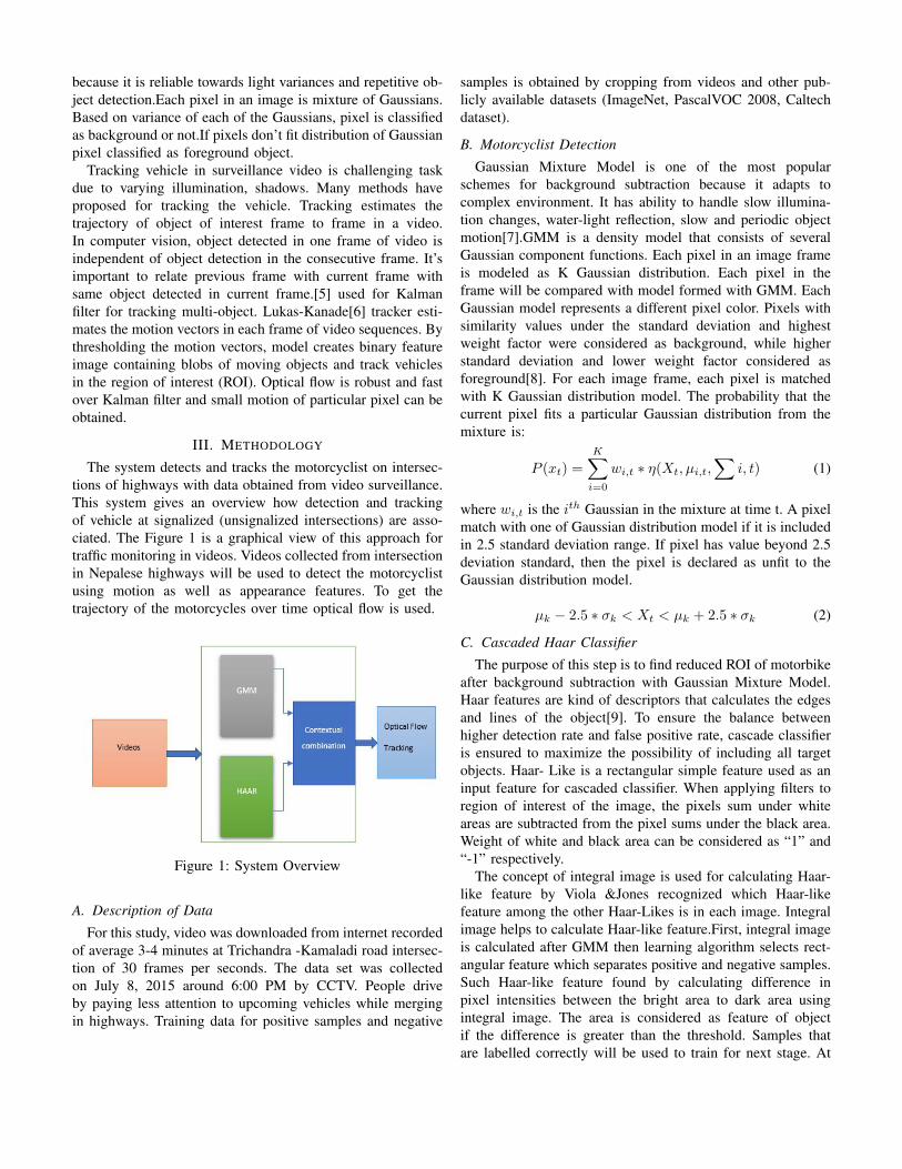
because it is reliable towards light variances and repetitive ob-ject detection.Each pixel in an image is mixture of Gaussians.Based on variance of each of the Gaussians, pixel is classifiedas background or not.If pixels don’t fit distribution of Gaussianpixel classified as foreground object.
Tracking vehicle in surveillance video is challenging taskdue to varying illumination, shadows. Many methods haveproposed for tracking the vehicle. Tracking estimates thetrajectory of object of interest frame to frame in a video.In computer vision, object detected in one frame of video isindependent of object detection in the consecutive frame. It’simportant to relate previous frame with current frame withsame object detected in current frame.[5] used for Kalmanfilter for tracking multi-object. Lukas-Kanade[6] tracker esti-mates the motion vectors in each frame of video sequences. Bythresholding the motion vectors, model creates binary featureimage containing blobs of moving objects and track vehiclesin the region of interest (ROI). Optical flow is robust and fastover Kalman filter and small motion of particular pixel can beobtained.
III. METHODOLOGY
The system detects and tracks the motorcyclist on intersec-tions of highways with data obtained from video surveillance.This system gives an overview how detection and trackingof vehicle at signalized (unsignalized intersections) are asso-ciated. The Figure 1 is a graphical view of this approach fortraffic monitoring in videos. Videos collected from intersectionin Nepalese highways will be used to detect the motorcyclistusing motion as well as appearance features. To get thetrajectory of the motorcycles over time optical flow is used.
Figure 1: System Overview
A. Description of Data
For this study, video was downloaded from internet recordedof average 3-4 minutes at Trichandra -Kamaladi road intersec-tion of 30 frames per seconds. The data set was collectedon July 8, 2015 around 6:00 PM by CCTV. People driveby paying less attention to upcoming vehicles while mergingin highways. Training data for positive samples and negative
samples is obtained by cropping from videos and other pub-licly available datasets (ImageNet, PascalVOC 2008, Caltechdataset).
B. Motorcyclist Detection
Gaussian Mixture Model is one of the most popularschemes for background subtraction because it adapts tocomplex environment. It has ability to handle slow illumina-tion changes, water-light reflection, slow and periodic objectmotion[7].GMM is a density model that consists of severalGaussian component functions. Each pixel in an image frameis modeled as K Gaussian distribution. Each pixel in theframe will be compared with model formed with GMM. EachGaussian model represents a different pixel color. Pixels withsimilarity values under the standard deviation and highestweight factor were considered as background, while higherstandard deviation and lower weight factor considered asforeground[8]. For each image frame, each pixel is matchedwith K Gaussian distribution model. The probability that thecurrent pixel fits a particular Gaussian distribution from themixture is:
P (xt) =
K∑i=0
wi,t ∗ η(Xt, µi,t,∑
i, t) (1)
where wi,t is the ith Gaussian in the mixture at time t. A pixelmatch with one of Gaussian distribution model if it is includedin 2.5 standard deviation range. If pixel has value beyond 2.5deviation standard, then the pixel is declared as unfit to theGaussian distribution model.
µk − 2.5 ∗ σk < Xt < µk + 2.5 ∗ σk (2)
C. Cascaded Haar Classifier
The purpose of this step is to find reduced ROI of motorbikeafter background subtraction with Gaussian Mixture Model.Haar features are kind of descriptors that calculates the edgesand lines of the object[9]. To ensure the balance betweenhigher detection rate and false positive rate, cascade classifieris ensured to maximize the possibility of including all targetobjects. Haar- Like is a rectangular simple feature used as aninput feature for cascaded classifier. When applying filters toregion of interest of the image, the pixels sum under whiteareas are subtracted from the pixel sums under the black area.Weight of white and black area can be considered as “1” and“-1” respectively.
The concept of integral image is used for calculating Haar-like feature by Viola &Jones recognized which Haar-likefeature among the other Haar-Likes is in each image. Integralimage helps to calculate Haar-like feature.First, integral imageis calculated after GMM then learning algorithm selects rect-angular feature which separates positive and negative samples.Such Haar-like feature found by calculating difference inpixel intensities between the bright area to dark area usingintegral image. The area is considered as feature of objectif the difference is greater than the threshold. Samples thatare labelled correctly will be used to train for next stage. At

Figure 2: Different Kinds of filters based on Haar-Like Fea-tures [10]
the end after a number of stages, strong cascade classifier isdeveloped. Cascaded classifier improves the processing speed.At first, using Viola Jones algorithm in motorcyclist detection,cascade file is trained separately by OpenCV and XML isprovided. Haar feature is trained with 990 positive and 5000negative samples of image dataset and XML files. This helpsto classify motorcyclist from non-motorcyclist type.
D. Contextual Combination
Both GMM and Haar-like features work in entirely differentprinciples as motion-based vs appearance based. Such asarticle[4][8]found motion to be more suitable for detectingtraffic than appearance, however, in our case a motorcyclistmight come to state of rest while merging where motiondetection might failed to detect those vehicles in rest so we areusing the appearance features. When both of them are acting,we draw a reliable bounding box for detecting motorcyclistusing haar and GMM.
E. Motorcyclist Tracking
Tracking estimates the trajectory of object of interestthroughout the video. GMM and Haar features used for de-tection, and vehicles (motorcycles) is tracked on the detectioninformation available in this system. When an object is trackedwhich was detected in previous frame, the appearance ofobject is a lot known. Tracking an object uses informationwhile detection starts from scratch. For this Lucas-Kanadeoptical flow method is used which detects whether new bikeor previous being tracked bike. New BikeID is assigned toevery new detected bike and tracker is deleted after the bikeleaves the frame.
IV. RESULTS AND DISCUSSIONS
Detection algorithm and tracking algorithm is applied to testvideo. At first test video is applied to Gaussian Mixture Modelwhich separates foreground from frame of video. Then Haaralgorithm is used to extract features from GMM processedframe. After applying contextual combination of detectionalgorithms, multiple bikes are detected.
Figure 3: Detecting motorbike after applying Haar algorithm
Figure 4: Motorbike ID 1 Tracking Result
In figure 4, yellow dot line shows the trajectory of bike ID 1while tracking.Motorbike tracking determines the ability of thesystem in tracking after detection. This tracking follows afterthe result of detection. When there are multiple motorbikespresent in frame of video , then it tracks those motorbikesassigning unique bike ID.
Figure 5: Two Motorbikes being tracked

Figure 6: Another example of Multiple Motorbikes beingtracked
Figure 7: Bike detected and tracked - previously not tracked
Bike which is in motion near by blue microbus is notdetected at this frame but it is detected and tracked in otherframes Figure 7. Bike should be detected as it enters the framebut this system detects and tracks bike in some other pointrather than entry point. So in tracking figures, yellow dot linesof trajectory of bike begins at other point than entry point. Ifa bike’s tracking doesn’t begin at entry point of frame, it isdetected and tracked at other frames of a video.
To evaluate the classifiers performance, recall, precision andaccuracy were used. True Positive (TP), number of imagescorrectly classified as motorcycles; false positives (FP), thenumber of images wrongly classified as motorcycles; falsenegative(FN), the number of images wrongly classified asnon-motorcycles and true negative(TN), the number of imagescorrectly classified as non-motorcycle.
Recall =TP
TP + FN(3)
Precision =TP
TP + FP(4)
Accuracy =TP + TN
TP + FP + FN + TN(5)
F1 = 2 ∗ Precision ∗RecallPrecision+Recall
(6)
Table I: Result of Bike Detection
True Positive(TP) True Negative(TN) False Positive(FP) FN24 0 16 3
Recall (Sensitivity) = 0.89Precision = 0.6F1-Score = 0.72False positive detections is high in algorithm. Such falsepositives is minimized while tracking such detection by opticalflow.
Table II: Bike Tracking Testing Result
Tracked True Positive(TP) True Negative(TN) False Positive(FP) FN21 20 0 1 3
Recall (Sensitivity)= 86.96%Precision = 95.23%F1-Score= 0.91Accuracy = 83.3 %The accuracy of bike tracking obtained is 83.3%. The bike thatis detected and tracked at the frame is counted. The calculationof motorcycle occurs if the motorcycle is detected as newobject rather than the motorcycle similar to existing bike onthe previous frame.
V. CONCLUSION
In this paper, video at intersections of road is providedsurveillance level view of motorbikes for different computervision algorithms. Adaboost cascaded Haar classifier usingHaar features is implemented with background detection.Incorporating optical flow tracking on contextual combina-tion of HAAR and GMM not only increases the sensitivity,precision, F1-score but also increases accuracy than Haardetection. Since high false positive in Haar detection only,object detection is checked at every 30 frames for trackingpurpose. While doing this approach,very few bikes are missedin detection. Optical flow was found to be better at rejectingnoisy detections.
Finally a method is demonstrated to a surveillance sceneusing contextual combination of detection and optical flowtracking results.
REFERENCES
[1] B. T. Morris and M. M. Trivedi. Learning, modeling, andclassification of vehicle track patterns from live video.Trans. Intell. Transport. Sys., 9(3):425–437, September2008.
[2] Sokemi Rene Emmanuel Datondji, Yohan Dupuis, PeggySubirats, and Pascal Vasseur. A survey of vision-basedtraffic monitoring of road intersections. Trans. Intell.Transport. Sys., 17(10):2681–2698, October 2016.
[3] Navneet Dalal and Bill Triggs. Histograms of orientedgradients for human detection. In Proceedings of the2005 IEEE Computer Society Conference on ComputerVision and Pattern Recognition (CVPR’05) - Volume 1 -
Volume 01, CVPR ’05, pages 886–893, Washington, DC,USA, 2005. IEEE Computer Society.
[4] Indrabayu, Rizki Yusliana Bakti, Intan Sari Areni, andA. Ais Prayogi. Vehicle detection and tracking usinggaussian mixture model and kalman filter. In 2016International Conference on Computational Intelligenceand Cybernetics. IEEE, 2016.
[5] Xin Li, Kejun Wang, Wei Wang, and Yang Li. Amultiple object tracking method using kalman filter. InThe 2010 IEEE International Conference on Informationand Automation. IEEE, jun 2010.
[6] Simon Baker and Iain Matthews. Lucas-kanade 20 yearson: A unifying framework. International Journal ofComputer Vision, 56(3):221–255, feb 2004.
[7] Juana E. Santoyo-Morales and Rogelio Hasimoto-Beltran. Video background subtraction in complex envi-ronments. Journal of Applied Research and Technology,12(3):527–537, jun 2014.
[8] A. Nurhadiyatna, B. Hardjono, A. Wibisono, I. Sina,W. Jatmiko, M. A. Ma’sum, and P. Mursanto. Improvedvehicle speed estimation using gaussian mixture modeland hole filling algorithm. In 2013 International Con-ference on Advanced Computer Science and InformationSystems (ICACSIS), pages 451–456, Sept 2013.
[9] Yun Wei, Qing Tian, Jianhua Guo, Wei Huang, andJinde Cao. Multi-vehicle detection algorithm throughcombining harr and HOG features. Mathematics andComputers in Simulation, 155:130–145, jan 2019.
[10] Mohammad Mahdi Moghimi, Maryam Nayeri, MajidPourahmadi, and Mohammad Kazem Moghimi. Movingvehicle detection using adaboost and haar-like feature insurveillance videos. CoRR, abs/1801.01698, 2018.

A Methodological Approach For Analysis, Design And Deployment Of Data Warehousing And Business
Intelligence
Siddhartha Singh [email protected]
ABSTRACT
Leading organizations are using a set of theories and
technologies that converts raw data into useful information
for the business use. They are seeking new, smarter ways
to improve performance, grow revenue, develop stronger
customer relationships and increase workforce
effectiveness – and they expect individuals in every role to
contribute to these outcomes. Business intelligence is a key
factor in achieving such results because it supports
informed decision making at every level, enabling
managers, executives and knowledge workers to take the
most effective action in a given situation. This paper not
only explores the underlying issues and the development of
information technology that provide business intelligence
,it also provides an actionable insight on how to plan,
build, and deploy business intelligence and data
warehousing solutions.
KEYWORDS: Business Intelligence, Data
Warehouse, DBMS, ETL, OLTP, OLAP
1. INTRODUCTION:
The principal reason why businesses need to create Data
Warehouses is that their corporate data assets are
fragmented across multiple, disparate applications systems,
running on different technical platforms in different
physical locations. This situation does not enable good
decision making. When data redundancy exists in multiple
databases, data quality often deteriorates. Poor business
intelligence results in poor strategic and tactical decision
making. Individual business units within an enterprise are
designated as "owners" of operational applications and
databases. These "organizational silos" sometimes don't
understand the strategic importance of having well
integrated, non-redundant corporate data. Consequently,
they frequently purchase or build operational systems that
do not integrate well with existing systems in the business. Due to globalization, mergers and outsourcing trends, the
need to integrate operational data from external
organizations has arisen. The sharing of customer and
sales data among business partners can, for example,
increase business intelligence for all business partners.
The challenge for Data Warehousing is to be able to
quickly consolidate, cleanse and integrate data from
multiple, disparate databases that run on different technical
platforms in different geographical locations.
2. BI CONCEPT:
The concept of Business Intelligence (BI) is brought up by
Gartner Group since 1996. It is defined as the application
of a set of methodologies and technologies, such as J2EE,
DOTNET, Web Services, XML, data warehouse, OLAP,
Data Mining, representation technologies, etc, to improve
enterprise operation effectiveness, support
management/decision to achieve competitive advantages.
Business Intelligence by today is never a new technology
instead of an integrated solution for companies, within
which the business requirement is definitely the key factor
that drives technology innovation. How to identify and
creatively address key business issues is therefore always
the major challenge of a BI application to achieve real
business impact. (Golfarelli et.al, 2004) defined BI that
includes effective data warehouse and also a reactive
component capable of monitoring the time critical
operational processes to allow tactical and operational
decision-makers to tune their actions according to the
company strategy.(Gangadharan and Swamy, 2004) define
BI as the result of in-depth analysis of detailed business
data, including database and application technologies, as
well as analysis practices. (Gangadharan and Swamy,
2004) widen the definition of BI as technically much
broader tools, that includes potentially encompassing
knowledge management, enterprise resource planning,
decision support systems and data mining. BI includes
several software for Extraction, Transformation and
Loading (ETL), data warehousing, database query and
reporting, (Berson et.al, 2002; Curt Hall, 1999)
multidimensional/on-line analytical processing (OLAP)
data analysis, data mining and visualization. The
capabilities of BI include decision support, online
analytical processing, statistical analysis, forecasting, and
data mining.
3. BI COMPONENTS:
3.1. Advanced Analytics:
It is referred to as data mining, forecasting or predictive
analytics, this takes advantage of statistical analysis

techniques to predict or provide certainty measures on
facts.
3.2. Corporate Performance Management (Portals,
Scorecards, Dashboards):
This general category usually provides a container for
several pieces to plug into so that the aggregate tells a
story. For example, a balanced scorecard that displays port
lets for financial metrics combined with say organizational
learning and growth metrics.
3.3. Conformed Dimension:
A conformed dimension is a set of data attributes that have
been physically implemented in multiple database tables
using the same structure, attributes, domain values,
definitions and concepts in each implementation.
Unlike in operational systems where data redundancy is
normally avoided, data replication is expected in the Data
Warehouse world. To provide fast access and intuitive
"drill down" capabilities of data originating from multiple
operational systems, it is often necessary to replicate
dimensional data in Data Warehouses and in Data Marts. Un-conformed dimensions imply the existence of logical
and/or physical inconsistencies that should be avoided.
3.4. Data Warehouse and data marts:
The data warehouse is the significant component of
business intelligence. It is subject oriented, integrated. The
data warehouse supports the physical propagation of data
by handling the numerous enterprise records for
integration, cleansing, aggregation and query tasks. It can
also contain the operational data which can be defined as
an updateable set of integrated data used for enterprise
wide tactical decision-making of a particular subject area.
It contains live data, not snapshots, and retains minimal
history. Data sources can be operational databases,
historical data, external data for example, from market
research companies or from the Internet), or information
from the already existing data warehouse environment. The
data sources can be relational databases or any other data
structure that supports the line of business applications.
They also can reside on many different platforms and can
contain structured information, such as tables or
spreadsheets, or unstructured information, such as plaintext
files or pictures and other multimedia information. A data
mart as described by (Inmon, 1999) is a collection of
subject areas organized for decision support based on the
needs of a given department. Finance has their data mart,
marketing has theirs, and sales have theirs and so on. And
the data mart for marketing only faintly resembles anyone
else's data mart. Perhaps most importantly, (Inmon, 1999)
the individual departments own the hardware, software,
data and programs that constitute the data mart. Each
department has its own interpretation of what a data mart
should look like and each department's data mart is
peculiar to and specific to its own needs. Similar to data
warehouses, data marts contain operational data that helps
business experts to strategize based on analyses of past
trends and experiences. The key difference is that the
creation of a data mart is predicated on am specific,
predefined need for a certain grouping and configuration of
select data. There can be multiple data marts inside an
enterprise. A data mart can support a particular business
function, business process or business unit. A data mart as
described by (Inmon, 1999) is a collection of subject areas
organized for decision support based on the needs of a
given department. Finance has their data mart, marketing
has theirs, and sales have theirs and so on. And the data
mart for marketing only faintly resembles anyone else's
data mart. BI tools are widely accepted as a new
middleware between transactional applications and
decision support applications, thereby decoupling systems
tailored to an efficient handling of business transactions
from systems tailored to an efficient support of business
decisions.
3.5. Data Sources:
Data sources can be operational databases, historical data,
external data for example, from market research companies
or from the Internet), or information from the already
existing data warehouse environment. The data sources can
be relational databases or any other data structure that
supports the line of business applications. They also can
reside on many different platforms and can contain
structured information, such as tables or spreadsheets, or
unstructured information, such as plaintext files or pictures
and other multimedia information.
3.6. Information Databases:
3.6.1. OLAP (On-line analytical processing):
It refers to the way in which business users can slice and
dice their way through data using sophisticated tools that
allow for the navigation of dimensions such as time or
hierarchies. Online Analytical Processing or OLAP
provides multidimensional, summarized views of business
data and is used for reporting, analysis, modeling and
planning for optimizing the business. OLAP techniques
and tools can be used to work with data warehouses or data
marts designed for sophisticated enterprise intelligence
systems. These systems process queries required to
discover trends and analyze critical factors. Reporting
software generates aggregated views of data to keep the
management informed about the state of their business.
Other BI tools are used to store and analyze data, such as
data mining and data warehouses; decision support systems
and forecasting; document warehouses and document
management; knowledge management; mapping,
information visualization, and dash boarding; management
information systems, geographic information systems;
Trend Analysis; Software as a Service (SaaS).
3.6.1.1. Data Cubes:
The main component of these systems is a OLAP cube. A
cube consists in combining data warehouse’s structures
like facts and dimensions. Those are organized as schemas:
star schema, snowflake schema and fact constellation. The
merging of all the cubes creates a multidimensional data
warehouse.
3.6.2. OLTP (On-line transaction processing):
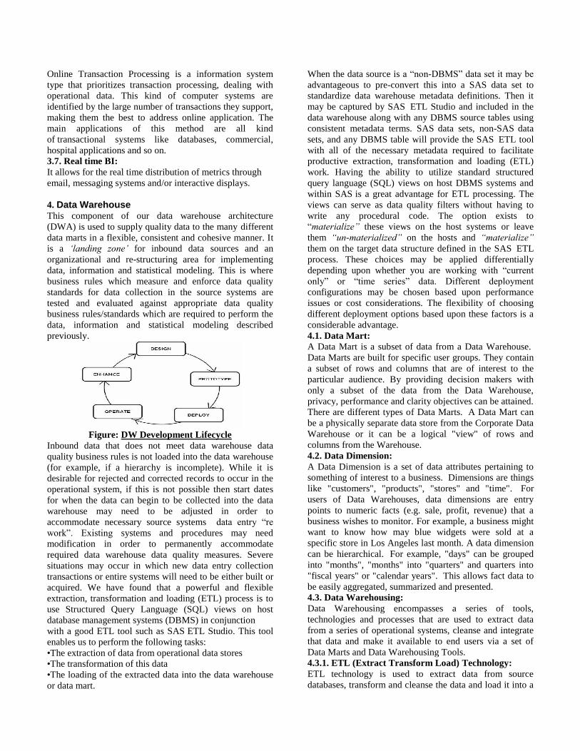
Online Transaction Processing is a information system
type that prioritizes transaction processing, dealing with
operational data. This kind of computer systems are
identified by the large number of transactions they support,
making them the best to address online application. The
main applications of this method are all kind
of transactional systems like databases, commercial,
hospital applications and so on.
3.7. Real time BI:
It allows for the real time distribution of metrics through
email, messaging systems and/or interactive displays.
4. Data Warehouse This component of our data warehouse architecture
(DWA) is used to supply quality data to the many different
data marts in a flexible, consistent and cohesive manner. It
is a ‘landing zone’ for inbound data sources and an
organizational and re-structuring area for implementing
data, information and statistical modeling. This is where
business rules which measure and enforce data quality
standards for data collection in the source systems are
tested and evaluated against appropriate data quality
business rules/standards which are required to perform the
data, information and statistical modeling described previously.
Figure: DW Development Lifecycle
Inbound data that does not meet data warehouse data
quality business rules is not loaded into the data warehouse
(for example, if a hierarchy is incomplete). While it is
desirable for rejected and corrected records to occur in the
operational system, if this is not possible then start dates
for when the data can begin to be collected into the data
warehouse may need to be adjusted in order to
accommodate necessary source systems data entry “re
work”. Existing systems and procedures may need
modification in order to permanently accommodate
required data warehouse data quality measures. Severe
situations may occur in which new data entry collection
transactions or entire systems will need to be either built or
acquired. We have found that a powerful and flexible
extraction, transformation and loading (ETL) process is to
use Structured Query Language (SQL) views on host
database management systems (DBMS) in conjunction
with a good ETL tool such as SAS ETL Studio. This tool
enables us to perform the following tasks:
•The extraction of data from operational data stores
•The transformation of this data
•The loading of the extracted data into the data warehouse
or data mart.
When the data source is a “non-DBMS” data set it may be
advantageous to pre-convert this into a SAS data set to
standardize data warehouse metadata definitions. Then it
may be captured by SAS ETL Studio and included in the
data warehouse along with any DBMS source tables using
consistent metadata terms. SAS data sets, non-SAS data
sets, and any DBMS table will provide the SAS ETL tool
with all of the necessary metadata required to facilitate
productive extraction, transformation and loading (ETL)
work. Having the ability to utilize standard structured
query language (SQL) views on host DBMS systems and
within SAS is a great advantage for ETL processing. The
views can serve as data quality filters without having to
write any procedural code. The option exists to
“materialize” these views on the host systems or leave
them “un-materialized” on the hosts and “materialize”
them on the target data structure defined in the SAS ETL
process. These choices may be applied differentially
depending upon whether you are working with “current
only” or “time series” data. Different deployment
configurations may be chosen based upon performance
issues or cost considerations. The flexibility of choosing
different deployment options based upon these factors is a
considerable advantage.
4.1. Data Mart:
A Data Mart is a subset of data from a Data Warehouse.
Data Marts are built for specific user groups. They contain
a subset of rows and columns that are of interest to the
particular audience. By providing decision makers with
only a subset of the data from the Data Warehouse,
privacy, performance and clarity objectives can be attained.
There are different types of Data Marts. A Data Mart can
be a physically separate data store from the Corporate Data
Warehouse or it can be a logical "view" of rows and
columns from the Warehouse.
4.2. Data Dimension:
A Data Dimension is a set of data attributes pertaining to
something of interest to a business. Dimensions are things
like "customers", "products", "stores" and "time". For
users of Data Warehouses, data dimensions are entry
points to numeric facts (e.g. sale, profit, revenue) that a
business wishes to monitor. For example, a business might
want to know how may blue widgets were sold at a
specific store in Los Angeles last month. A data dimension
can be hierarchical. For example, "days" can be grouped
into "months", "months" into "quarters" and quarters into
"fiscal years" or "calendar years". This allows fact data to
be easily aggregated, summarized and presented.
4.3. Data Warehousing:
Data Warehousing encompasses a series of tools,
technologies and processes that are used to extract data
from a series of operational systems, cleanse and integrate
that data and make it available to end users via a set of
Data Marts and Data Warehousing Tools.
4.3.1. ETL (Extract Transform Load) Technology:
ETL technology is used to extract data from source
databases, transform and cleanse the data and load it into a
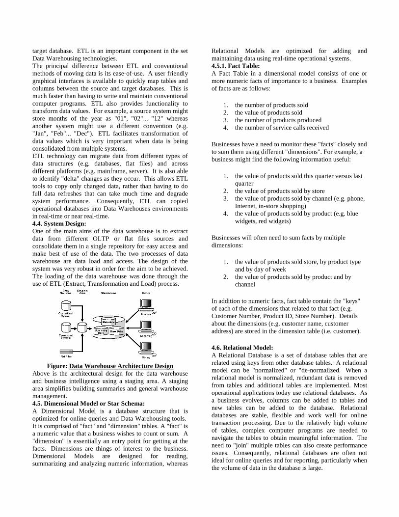
target database. ETL is an important component in the set
Data Warehousing technologies.
The principal difference between ETL and conventional
methods of moving data is its ease-of-use. A user friendly
graphical interfaces is available to quickly map tables and
columns between the source and target databases. This is
much faster than having to write and maintain conventional
computer programs. ETL also provides functionality to
transform data values. For example, a source system might
store months of the year as "01", "02"... "12" whereas
another system might use a different convention (e.g.
"Jan", "Feb"... "Dec"). ETL facilitates transformation of
data values which is very important when data is being
consolidated from multiple systems.
ETL technology can migrate data from different types of
data structures (e.g. databases, flat files) and across
different platforms (e.g. mainframe, server). It is also able
to identify "delta" changes as they occur. This allows ETL
tools to copy only changed data, rather than having to do
full data refreshes that can take much time and degrade
system performance. Consequently, ETL can copied
operational databases into Data Warehouses environments
in real-time or near real-time.
4.4. System Design:
One of the main aims of the data warehouse is to extract
data from different OLTP or flat files sources and
consolidate them in a single repository for easy access and
make best of use of the data. The two processes of data
warehouse are data load and access. The design of the
system was very robust in order for the aim to be achieved.
The loading of the data warehouse was done through the
use of ETL (Extract, Transformation and Load) process.
Figure: Data Warehouse Architecture Design
Above is the architectural design for the data warehouse
and business intelligence using a staging area. A staging
area simplifies building summaries and general warehouse
management.
4.5. Dimensional Model or Star Schema:
A Dimensional Model is a database structure that is
optimized for online queries and Data Warehousing tools.
It is comprised of "fact" and "dimension" tables. A "fact" is
a numeric value that a business wishes to count or sum. A
"dimension" is essentially an entry point for getting at the
facts. Dimensions are things of interest to the business. Dimensional Models are designed for reading,
summarizing and analyzing numeric information, whereas
Relational Models are optimized for adding and
maintaining data using real-time operational systems.
4.5.1. Fact Table:
A Fact Table in a dimensional model consists of one or
more numeric facts of importance to a business. Examples
of facts are as follows:
1. the number of products sold
2. the value of products sold
3. the number of products produced
4. the number of service calls received
Businesses have a need to monitor these "facts" closely and
to sum them using different "dimensions". For example, a
business might find the following information useful:
1. the value of products sold this quarter versus last
quarter
2. the value of products sold by store
3. the value of products sold by channel (e.g. phone,
Internet, in-store shopping)
4. the value of products sold by product (e.g. blue
widgets, red widgets)
Businesses will often need to sum facts by multiple
dimensions:
1. the value of products sold store, by product type
and by day of week
2. the value of products sold by product and by
channel
In addition to numeric facts, fact table contain the "keys"
of each of the dimensions that related to that fact (e.g.
Customer Number, Product ID, Store Number). Details
about the dimensions (e.g. customer name, customer
address) are stored in the dimension table (i.e. customer).
4.6. Relational Model:
A Relational Database is a set of database tables that are
related using keys from other database tables. A relational
model can be "normalized" or "de-normalized. When a
relational model is normalized, redundant data is removed
from tables and additional tables are implemented. Most
operational applications today use relational databases. As
a business evolves, columns can be added to tables and
new tables can be added to the database. Relational
databases are stable, flexible and work well for online
transaction processing. Due to the relatively high volume
of tables, complex computer programs are needed to
navigate the tables to obtain meaningful information. The
need to "join" multiple tables can also create performance
issues. Consequently, relational databases are often not
ideal for online queries and for reporting, particularly when
the volume of data in the database is large.

Most Data Warehousing applications, therefore, are built
using dimensional models.
4.7. Meta Data:
Meta data is simply data about data. It includes a
definition of each field in the Data Warehouse and the
corresponding domain values. Meta data describes where
the data came from and how it was transformed or cleansed
during the data integration process. Because warehouse
data can originate from multiple sources and is used for
critical decision making, it is important that data
definitions be clear and accessible to all Data Warehouse
users.
5. ANALYSIS-DESIGN-DEPLOYMENT TOOLS:
The tools discussed here are front-end tools that are
available to transform data in a Data Warehouse into
actionable business intelligence. The use of appropriate
Data Warehousing tools can help ensure that the right
information gets to the right person via the right channel at
the right time.
5.1. Automated Alerts:
Custom built and purchased application systems can be
implemented to examine data in a Data Warehouse and
initiate system generated alerts when predefined thresholds
are reached, or when expected results are not attained.
Alerts can be sent via an email, phone message or an
electronic workflow item to the appropriate decision
maker. The rules for triggering automated alerts can easily
be adjusted as business requirements change.
5.2. Data Mining Tools:
Data Mining Tools are analytical engines that use data in a
Data Warehouse to discover underlying correlations. Data
Mining Tools are used by analysts to gain business
intelligence by identifying and observing trends, problems
and anomalies. Because the business environment is so
dynamic, it is often difficult for businesses to quickly
identify emerging patterns or trends. Data Mining Tools
help businesses identify problems and opportunities
promptly and then make quick and appropriate decisions
with the new business intelligence.
5.3. Excel Spreadsheets:
These are frequently used in Data Warehousing
applications to access and present data from Data Marts.
Spreadsheets are powerful, flexible and relatively
inexpensive tools that many decision makers are
comfortable using. Before Data Warehousing became
popular, decision makers often had difficulty getting access
to corporate data. It was necessary to populate spreadsheets
from multiple disparate data sources and manually
integrate the data. This process was both time consuming
and error-prone.
The use of Excel Spreadsheets to present and analyze data
from Data Warehouses is an inexpensive and flexible
method for sharing business intelligence.
5.4. OLAP Tools:
These are used to analyze multi-dimensional data and
allow users to identify observe trends and then to "drill-
down" to discover the details behind those trends. As the
name implies, OLAP tools are "online" and are used for
"analytics". Many firms are addressing their information
needs by replacing their static, paper-based legacy reports
with online access to corporate information via OLAP
Tools.
5.5. Dashboards:
Performance Dashboards are targeted at senior decision
makers who need to know at a glance, how the business is
performing against its measurable goals and objectives. The performance measures shown on Dashboards are
based on the firm's key performance indicators (KPIs).
KPIs can involve financial, marketing, production,
customer, growth and other important metrics.
6. Data Warehouse & BI solution BENIFITS:
Once a data warehouse is in place and populated with data,
it will become a part of a BI solution that will deliver
benefits to business users in many ways:
▪ End user creation of reports: The creation of
reports directly by end users is much easier to
accomplish in a BI environment. They can also
create much more useful reports because of the
power and capability of BI tools compared to a
source application. And moving the creation of
reports to a BI system increases consistency and
accuracy and usually reduces cost.
▪ Ad-hoc reporting and analysis: Since the data
warehouse eliminates the need for BI tools to
compete with the transactional source systems,
users can analyze data faster and generate reports
more easily, and slice-and-dice in ways they could
never do before. The Microsoft BI toolset vastly
improves the ability to analyze data.
▪ Dynamic presentation through dashboards:
Managers want access to an interactive display of
up-to-date critical management data. That is
accomplished via dashboards, which are
sophisticated displays that show information in
creative and highly graphical forms, much like the
instrument panel on an automobile.
▪ Drill-down capability: Users can drill down into
the details underlying the summaries on
dashboards and reports. The allows users to slice
and dice to find underlying problems.
▪ Support for regulations: Sarbanes-Oxley and
other related regulations have requirements that
transactional systems are sometimes not able to
support. With a data warehouse, the necessary
data can be retained as long as the law requires
▪ Metadata creation: Descriptions of the data can
be stored with the data warehouse to make it a lot
easier for users to understand the data in the
warehouse. This will make report creation much
simpler for the end-user

▪ Support for operational processes: A data
warehouse can help support business needs, such
as the ability to consolidate financial results
within a complex company that uses different
software for different divisions
▪ Data mining: Once you have built out a data
warehouse, there are data mining tools that you
can use to help find hidden patterns using
automatic methodologies. While reporting tools
can tell you where you have been, data mining
tools can tell you where you are going.
▪ Security: A data warehouse makes it much easier
to provide secure access to those that have a
legitimate need to specific data and to exclude
others.
▪ Analytical tool support: There are many vendors
who have analytical tools (i.e. QlikView, Tableau)
that allow business units to slice and dice the data
and create reports and dashboards. These tools
will all work best when extracting data from a
data warehouse.
This long list of benefits is what makes BI based on a data
warehouse an essential management tools for companies.
7. IMPORTANCE:
A goal of every business is to make better business
decisions than their competitors. That is where business
intelligence (BI) comes in. BI turns the massive amount of
data from operational systems into a format that is easy to
understand, current, and correct so decisions can be made
on the data. You can then analyze current and long-term
trends, be instantly alerted to opportunities and problems,
and receive continuous feedback on the effectiveness of
your decisions. In absence of BI, probably it wouldn't be
possible to identify the root cause or even if it is found out,
it would probably be difficult to identify the bleeding
points and the business organizations may end up taking
corrective actions in all territories which probably would
cause another problems. Thus, BI just enables to find out
right information, to the right person, at the right time, at
the right place to help and improve the informed decision
making in order to solve the issues business might be
facing. So, it is not just a solution to any business
problems, it is kind of a tool or a step to identify and solve
the required problems for an effective outcome.
8. CONCLUSION:
Companies that build data warehouses and use business
intelligence for decision-making ultimately save money
and increase profit. Timely foundation and feedback
information is needed as part of that effective decision
making with the help of different tools. Hence, the paper is
to help the decision makers of the company making an
effective decision. Therefore, we need to make business
intelligence available throughout the organization to
explore how to define and specify useful management
reports from warehouse data.
REFERENCES: [1] Eldabi, T., et al (2002), Quantitative and qualitative decision
making methods in simulation modeling. Management Decision,
Vol.40(1) p. 64-73.
[2]Giovinazzo, W (2002), ‘Internet-Enabled Business
Intelligence’, Prentice Hall.
[3] Kimball R. and Ross M., (2002) the Data Warehouse Toolkit:
Second Edition, the Complete Guide to Dimensional Modeling.
[4] Debbie Weisensee, Implementing Data Warehousing and
Business Intelligence at McMaster University Using the SAS®
Intelligence Value Chain
[5]Chaffey, D. (2002). E-business and E-commerce management.
New York PrenticeHall, p 330-370
[6]Fox R., (2004) Moving from data to information OCLC
Systems and Services: International Digital Library Perspectives
Volume 20 Number 3 pp 96-101
[7]Başaran, Beril P (2005), a Comparison of Data Warehouse
Design Models, the Graduate School of Natural and Applied
Sciences, Atilim University
[8]Inmon W.H., (1993) Building the Data Warehouse, A Wiley
QED publication, John Wiley and Sons, Inc. New York 123-133
[9]Matteo Golfarelli. (2004) DEIS - University of
Bologna,”Beyond data warahousing”
[10] Oracle Database 11g for Data Warehousing and Business
Intelligence.
[11]Gangadharan & Swamy (2004), “Buisness Intelligence
systems:design & implementing strategies”.
[12]Poe, V., et al (1997). Building a DataWarehouse for Decision
Support 2nd ed., Prentice Hall .
[13] Maria Sueli Almeida, Getting Started with DataWarehouse
and Business Intelligence.
[14]Berson Alex, Smith Stephen and Thearling Kurt. (2002)
‘Building Data Mining Applications for CRM’.
[15]Data Warehouse Architecture Design Figures,Oracle
Database Online Documentation 12c Release 1 (12.1).
[16] Inmon W.H., (1993) Building the Operational Data Store”,
Wiley Publishers-New York,2nd edition.
[17] Davenport, T.H.(1993) ‘Process Innovation: Reengineering
Work through Information Technology’, Harvard Business
School Press, Boston.
[18]Malhotra, Y. (2000) ‘information management to knowledge
management: Beyond “Hi-Tech Hidebound” systems’, in
Srikantaiah, T. K. and Koenig, M.E.D. (Eds.) Knowledge
Management, Medford,NJ.
[19]Hall,H(1999),”Online Information Sources”,Journal of
Information Science,(26)3,pp.139
[20] www.ibm.com/business_intelligence
[21] www.saycocorporativo.com/saycouk/bij/journals

Pattern Recognition for Cercospora Coffeicola in Coffee
Plant
Swarup Raj Dhungana
[email protected], +977-9843074784
Abstract
In the current context of Nepal, coffee cultivation is
one of the major cash crops cultivated most widely
across the country. In spite of being cultivated
extensively the yield and growth of coffee are found to
be inadequate due to different reasons like old
techniques of cultivation, infection, climate change
and so on. The main aim of this study is to use the
pattern recognition technique to detect a specific plant-
pathogen Cercospora Coffeicola in coffee plant and
prevent from leaf spots and berry blotch disease in the
plant. The TensorFlow framework with Mask R-CNN
would help to detect the lesions at the pixel level to
provide more accurate results.
Introduction
According to the “Statistical Information On Nepalese
Agriculture” (015/016) by Ministry of Agriculture
Development, more than thirty thousand farmers are
directly involved with coffee farming in Nepal. Coffee
cultivation has been one of the most effective cash
crops with its farming widely spread in more than 40
districts of Nepal. Although widely cultivated and
highly effective cash crop at times creates a huge
problem for the farmers to get the maximum yield and
good quality beans because of some common yet hard
to diagnose diseases in the plants.
Cercospora coffeicola is a plant-pathogenic fungus
which affects almost 70% of the coffee cultivation
worldwide. The fungus is responsible for a common
disease Cercospora leaf spot which if ignored, later
enhances into berry blotch (a condition where the
proper growth of the coffee berries is effected). The
disease is considered to have a huge economic impact
for the farmers due to its damaging effects on plants,
yield and the quality of the beans.
The main aim of the research is to train a model to
recognize the pattern at early stage of the Cerscospora
leaf spot and prevent from further damage of the
coffee beans. Since the pattern recognition must be
done minutely at the pixel level, Mask R-CNN would
be one of the most suitable model for training.
Source: Towards Data Science
Mask R-CNN is a simple upgrade to the Faster R-
CNN, a Faster R-CNN returns a class name and the
bounding boxes for each detected objects whereas
Mask R-CNN returns one more addition output i.e.
object mask which basically indicates the pixel level
where the object is actually placed. Training of the
model shall be conducted in TensorFlow frame work.
Diagnosis of Cercospora Coffeicola
Although the plant-pathogenic fungus is seen in many
different plant species but it has a similar diagnosis
and symptoms in all the plants, mostly seen on the
leaves of the effected ones.
The basic symptom is a circular shaped spot with gray
or white centers. The lesions are usually irregular
shaped and causes blight on the leaf, they appear as a
small, chlorotic presence on the upper leaf surface
which further expands to deep brown patches.
Moreover, leaf blight is not solely caused by
Cercospora Coffeicola which makes it difficult in
diagnosis process even if the leaf blight is seen in the
coffee plant the real cause cannot be confirmed easily.
The center of the leaf spots is grayish which are
encircled by a distinct ring of 0.2 – 0.6 inches in
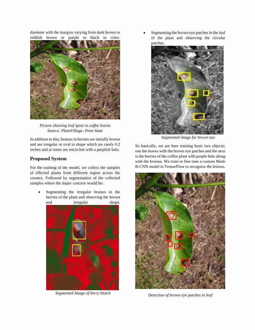
diameter with the margins varying from dark brown to
reddish brown or purple to black in color.
Picture showing leaf spots in coffee leaves
Source: PlantVillage- Penn State
In addition to this, bruises in berries are initially brown
and are irregular or oval in shape which are rarely 0.2
inches and at times are encircled with a purplish halo.
Proposed System
For the training of the model, we collect the samples
of effected plants from different region across the
country. Followed by segmentation of the collected
samples where the major concern would be:
Segmenting the irregular bruises in the
berries of the plant and observing the brown
and irregular shape.
Segmented Image of berry blotch
Segmenting the brown eye patches in the leaf
of the plant and observing the circular
patches.
Segmented image for brown eye
So basically, we are here training basic two objects;
one the leaves with the brown eye patches and the next
is the berries of the coffee plant with purple halo along
with the bruises. We train or fine tune a custom Mask
R-CNN model in TensorFlow to recognize the lesions.
Detection of brown eye patches in leaf
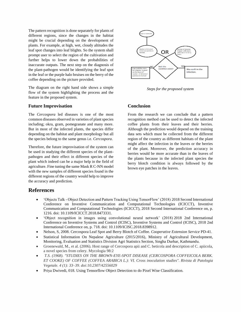
The pattern recognition is done separately for plants of
different regions, since the changes in the habitat
might be crucial depending on the development of
plants. For example, at high, wet, cloudy altitudes the
leaf spot changes into leaf blights. So the system shall
prompt user to select the region of the cultivation and
further helps to lower down the probabilities of
inaccurate outputs. The next step on the diagnosis of
the plant-pathogen would be identifying the leaf spot
in the leaf or the purple halo bruises on the berry of the
coffee depending on the picture provided.
The diagram on the right hand side shows a simple
flow of the system highlighting the process and the
feature in the proposed system.
Steps for the proposed system
Future Improvisation
The Cercospora led diseases is one of the most
common diseases observed in varieties of plant species
including; okra, gram, pomegranate and many more.
But in most of the infected plants, the species differ
depending on the habitat and plant morphology but all
the species belong to the same genus i.e. Cercospora.
Therefore, the future improvisation of the system can
be used in studying the different species of the plant-
pathogen and their effect in different species of the
plant which indeed can be a major help in the field of
agriculture. Fine tuning the same Mask R C-NN model
with the new samples of different species found in the
different regions of the country would help to improve
the accuracy and prediction.
Conclusion
From the research we can conclude that a pattern
recognition method can be used to detect the infected
coffee plants from their leaves and their berries.
Although the prediction would depend on the training
data sets which must be collected from the different
region of the country as different habitats of the plant
might affect the infection in the leaves or the berries
of the plant. Moreover, the prediction accuracy in
berries would be more accurate than in the leaves of
the plants because in the infected plant species the
berry blotch condition is always followed by the
brown eye patches in the leaves.
References
‘Objects Talk - Object Detection and Pattern Tracking Using TensorFlow’ (2018) 2018 Second International
Conference on Inventive Communication and Computational Technologies (ICICCT), Inventive
Communication and Computational Technologies (ICICCT), 2018 Second International Conference on, p.
1216. doi: 10.1109/ICICCT.2018.8473331.
‘Object recognition in images using convolutional neural network’ (2018) 2018 2nd International
Conference on Inventive Systems and Control (ICISC), Inventive Systems and Control (ICISC), 2018 2nd
International Conference on, p. 718. doi: 10.1109/ICISC.2018.8398912.
Nelson, S, 2008. Cercospora Leaf Spot and Berry Blotch of Coffee. Cooperative Extension Service PD-41.
Statistical Information On Nepalese Agriculture (2015/2016), Ministry of Agricultural Development,
Monitoring, Evaluation and Statistics Division Agri Statistics Section, Singha Durbar, Kathmandu.
Groenewald, M., et al. (2006). Host range of Cercospora apii and C. beticola and description of C. apiicola,
a novel species from celery. Mycologia 98:2
T.S. (1968). "STUDIES ON THE BROWN-EYE-SPOT DISEASE (CERCOSPORA COFFEICOLA BERK.
ET COOKE) OF COFFEE (COFFEA ARABICA L.): VI. Cross inoculation studies". Rivista di Patologia
Vegetale. 4 (1): 33–39. doi:10.2307/42556029
Priya Dwivedi, 018. Using Tensorflow Object Detection to do Pixel Wise Classification.

1
Development of Actuator interface circuit for portable device for
health monitoring of metallic structure
Manish Man Shrestha1*, Bibek Ropakheti2, Uddhav Bhattarai1, Ajaya Adhikari1
1Departent of Electronics and Communication Engineering, Cosmos College of Management and Technology,
Satdobato, Nepal 2Department of Computer Engineering, Cosmos College of Management and Technology, Satdobato, Nepal
*Corresponding author: phone 9840316635 e-mail [email protected]
━━━━━━━━━━━━━━━━━━━━━━━━━━━━━━━━
ABSTRACT
Damage detection of the metallic structures such as
hydro-powers pipelines, water supply pipelines and
bridges are the crucial issues in the modern world. The
early detection of the generation of cracks and corrosion
in such structures can prevent the unwanted accident and
can save the structures as well as human lives. One of the
widely used method in structural health monitoring is to
generate the lamb wave and to analyze the wave for
detection of damage in the structure. This paper
describes the generation of the actuation lamb wave
through low power portable device. The frequency and
amplitude of lamb wave plays a vital role to determine
the quantity and quantity of the damage in the structure.
The proposed device can generate up to the lamb wave
with central frequency of 137 kHz, 6-cycles and 10 Vp-
p amplitude. The device comprises of amplifier, signal
selective circuit and microcontroller with DMA
controller and DAC to generate, as well as, to control the
frequency of the actuated lamb wave. The generated
lamb wave can be further used with different sensors
such as Laser Doppler Velocimetry (LDV), Piezoelectric
(PZT), Micro electro mechanical system (MEMS)
accelerometer and so on for further analysis of the lamb
wave data.
Key Words: Structural health monitoring, damage
detection, lamb wave generation, lamb wave actuator
INTRODUCTION
The PZT excited structural health monitoring system is
one of the widely used and well proven technology in
research area of structural health monitoring [1~2]. The
size, weight and low cost of the PZT actuators make it
suitable to use it in low power and portable devices. With
the modern technologies, such as controller with low
power and high processing speed and wireless
communications, many researchers have inclined to the
development of smart technologies. Many researchers
have successfully integrated the modern technologies
with structural health monitoring system to develop
smart devices [3~5]. With further advancement of the
technologies, such as capability of the controller to
process the signal with floating point unit, the researcher
has further developed the intelligent system to monitor
the structure [6]. However, the PZT actuator developed
is either low in frequency or low in amplitude. Another
limitation found in smart or intelligent system is that it
uses single actuator to detect the damage in the structure.
It is well proven that the multiple actuator in the system
can not only detect the damage but also can localize it
[7]. This research tends to utilize modern technology
with the PZTs to develop an actuator circuit with
amplitude up to 15 Vp-p, frequency up to 137 kHz and
handles up to 8 actuators. The filter or signal selective
circuit is designed to filter out the aliasing noise. The
filter topology used in the circuit is multiple feedback
filter topology. The multiple feedback filter makes sure
that the sensitivity remains low even if there is variation
in component. The single end topology of the multiple
feedback filter also makes it suitable for shifting the
voltage level of the input signal by providing the suitable
voltage at the other end of the amplifier [8].
The circuit mainly consists of microcontroller and the
actuator circuit. The microcontroller fetches the
frequency and actuator information from the user, then
generates the lamb wave and send it to the desired
actuator. The actuation circuit amplifies, filters and shift
the voltage level of the lamb wave to make it compatible
with PZT actuators. The figure 1 shows the overview of
the system.
Figure 1 Overview
The in-built DSP (Digital Signal Processor) has been
used to generate the waveform data with precise
frequency information and the in-built DMA (Direct
Memory Access) transfer the waveform data from the
buffer to the DAC (Digital to Analog Converter) of the

2
microcontroller to produce an actual lamb wave from the
controller. The DSP is the processor that can fetch
multiple instructions at the same time, mainly used for
floating-point data, which results in precise frequency
information of the lamb wave. The DMA is the feature of
the controller that allows access to system bus of the
controller without the intervention of the core controller.
The programming flow of the controller is managed
through RTOS (Real Time Operating System). RTOS is
an operating system developed to manage the task of the
controller in real time applications, typically without any
buffer delays.
DEVELOPMENT OF ACTUATOR INTERFACE
CIRCUIT
For the development of the actuator interface circuit first
the firmware, then amplifier with filter and voltage level
shifting circuit were designed. The firmware was
developed using RTOS platform. The firmware’s flow is
controlled by three tasks of RTOS. First task is a simple
led status task, which shows the status of the system, i.e.
if the system is running or not, if the system is gathering
information from the user, or if the system is generating
actuation signal or not. Second task continuously
monitors the serial communication to gather the
information such as central frequency of the lamb wave,
number of actuators to actuate and which actuator to
actuate from the user. Third task generates the waveform
in accordance to the user information and selects the
desired actuator. The actuation wave is generated by
combining the exponential wave and cosine wave and
reversing it accordingly. The equation to generate the
wave is given by
Once the lamb wave is generated, the DMA (Direct
Memory Access) controller is triggered to transfer the
generated wave data in the buffer memory to the DAC
(Digital to Analog Converter), which in turn generates
the lamb wave. The maximum frequency that were
generated via controller is 137 kHz. The generated wave
is passed then passed through the amplifier with filter
and voltage level shifting circuit. The transfer function
of the actuator circuit is given by
The Bode-plot and Nyquist plot of the circuit is
shown in figure 2 and 3.
Figure 2 Bode plot
Figure 3 Nyquist plot
Two twelve-volt batteries have been used to power up the
device. The power consumption of the circuit during
actuation is 0.576 watt.
IMPLEMENTATION OF THE ACTUATOR
CIRCUIT
The circuit was first assembled and check for the lamb
wave generation. Figure below shows the lamb wave
generation circuit with anti-aliasing filter and amplifier.
As can be seen in the figure 4, the lamb wave generated
are high in amplitude and filtered in accordance to our
requirement.
Figure 4 Lamb wave generation
The signal was further tested with the actuator and sensor
system. The steel structure is used as test specimen. The
test configuration for the validation of the actuation
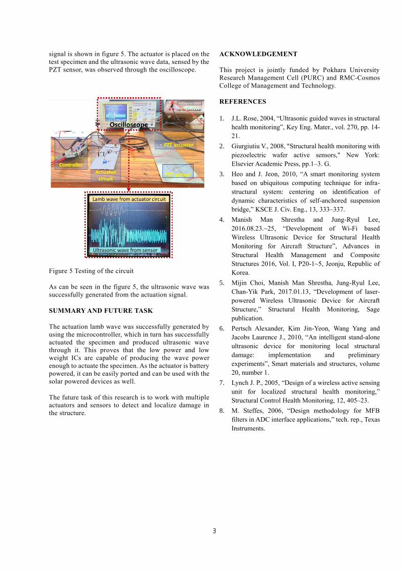
3
signal is shown in figure 5. The actuator is placed on the
test specimen and the ultrasonic wave data, sensed by the
PZT sensor, was observed through the oscilloscope.
Figure 5 Testing of the circuit
As can be seen in the figure 5, the ultrasonic wave was
successfully generated from the actuation signal.
SUMMARY AND FUTURE TASK
The actuation lamb wave was successfully generated by
using the microcontroller, which in turn has successfully
actuated the specimen and produced ultrasonic wave
through it. This proves that the low power and low
weight ICs are capable of producing the wave power
enough to actuate the specimen. As the actuator is battery
powered, it can be easily ported and can be used with the
solar powered devices as well.
The future task of this research is to work with multiple
actuators and sensors to detect and localize damage in
the structure.
ACKNOWLEDGEMENT
This project is jointly funded by Pokhara University
Research Management Cell (PURC) and RMC-Cosmos
College of Management and Technology.
REFERENCES
1. J.L. Rose, 2004, “Ultrasonic guided waves in structural
health monitoring”, Key Eng. Mater., vol. 270, pp. 14-
21.
2. Giurgiutiu V., 2008, "Structural health monitoring with
piezoelectric wafer active sensors," New York:
Elsevier Academic Press, pp.1–3. G.
3. Heo and J. Jeon, 2010, “A smart monitoring system
based on ubiquitous computing technique for infra-
structural system: centering on identification of
dynamic characteristics of self-anchored suspension
bridge,” KSCE J. Civ. Eng., 13, 333–337.
4. Manish Man Shrestha and Jung-Ryul Lee,
2016.08.23.~25, “Development of Wi-Fi based
Wireless Ultrasonic Device for Structural Health
Monitoring for Aircraft Structure”, Advances in
Structural Health Management and Composite
Structures 2016, Vol. I, P20-1~5, Jeonju, Republic of
Korea.
5. Mijin Choi, Manish Man Shrestha, Jung-Ryul Lee,
Chan-Yik Park, 2017.01.13, “Development of laser-
powered Wireless Ultrasonic Device for Aircraft
Structure,” Structural Health Monitoring, Sage
publication.
6. Pertsch Alexander, Kim Jin-Yeon, Wang Yang and
Jacobs Laurence J., 2010, “An intelligent stand-alone
ultrasonic device for monitoring local structural
damage: implementation and preliminary
experiments”, Smart materials and structures, volume
20, number 1.
7. Lynch J. P., 2005, “Design of a wireless active sensing
unit for localized structural health monitoring,”
Structural Control Health Monitoring, 12, 405–23.
8. M. Steffes, 2006, “Design methodology for MFB
filters in ADC interface applications,” tech. rep., Texas
Instruments.

XXX-X-XXXX-XXXX-X/XX/$XX.00 ©20XX IEEE
Bluetooth Smart: Rape Issues Solution
Sanjaya Shrestha
Bachelor of Engineering in Software Engineering(BESE)
Nepal College of Information and Technology(NCIT) (PU Affiliated) Lalitpur, Nepal 9861111815
AasmaSharma
Bachelor of Engineering in Software Engineering(BESE)
Nepal College of Information and Technology(NCIT) (PU Affliated) Lalitpur, Nepal 9868176258
Abstract—The world is now getting huge interest
on IoT and every day the no of IoT devices are
increasing. The environment around us is being
smarter through the IoT technology. The devices are
getting internet connectivity and making our
activities smarter and easier.
The IoT devices can be a very good solution for
controlling the today’s issues of insecurities like
rape, kidnap. In this paper we tried to highlight
some possibility of IoT in light of Bluetooth Smart as
a solution to such crime or actions and means of
saving lives.
Keywords—IoT, Bluetooth Smart, privacy and
security, Internet, IoT, Bluetooth Smart
I. INTRODUCTION
Internet of Things (IoT), refers to the devices with access of Internet. The term was first used in 1999 by Kevin Ashton, to connect objects to Internet.
Now We are in peak of using IoT devices for our daily actions, By means of sensors the objects are getting Internet Connectivity and now gathering data, analyzing and predicting the next sequence has been common.
Bluetooth Low Energy (BLE) a.k.a Bluetooth Smart, is now evolving as it is the one with low consumption of Energy. After introducing BLE in Bluetooth 4.2 and offering Internet Protocol (IP), we can now connect to other IoT devices. And the most competitive advantage is out of box support in most smart phones.
Bluetooth carries a good potential market in these IoT worlds, as It is also evolving through security, privacy and increased data rate and speed.
II. ISSUES ON IOT
A. Internet
Since IoT refers to connectivity of Internet, the dependency had increased a lot. For smallest act also, we use internet without considering the privacy and security. Since Internet is a global access which means vulnerable to our data gathered by IoT devices. In intra home activities also like switching, monitoring we use internet the most. This shows our dependency on Internet.
B. Energy and Bandwidth
Using Internet consumes more amount of Energy and also requires high bandwidth for transferring data. IoT needs to frequently communicate over Internet for analyzing and processing the data, which means continuous consumption of Energy.
C. Privacy and Security
The data gathered by IoT are distributed all over the Internet so It creates problem on privacy and security. As we depend most on Internet the small act can also be regulated by Internet with vulnerability of Profiling, Identification, Inventory Attack etc.
III. BLUETOOTH SMART
To overcome these issues in IoT, Bluetooth Smart can be a very good alternative of option to enhance the power of IoT. We can automate different activities with Bluetooth like home activities which maintains a good security and privacy.
A. Bluetooth smart and IoT
Introduction to Internet Protocol Support Profile (IPSP), enables an IPv6 enabled Bluetooth peripheral, and a mechanism to discover and establish a link layer connections. Bluetooth Gatt service called the HTTP Proxy Service has been standardized for the BLE connected IoT, which further complements the connectivity of BLE devices with the Internet
B. Improved privacy and less power
consumption
The privacy is increasingly threatened due to
increased IoT devices. The personal data can be
derived from sensors data, user data and other
sources. The privacy is too concerned with IoT
devices due to more personalized data.
Bluetooth can operate from hours to month in a coin
cell battery, Hence, it can stand as a good lasting
resource for transmitting signal.
IV. BLUETOOTH SMART USECASES
Bluetooth is operable in a coin size battery for hours to month, so we are using it as a medium for transferring signal between peer to peer. The range of Bluetooth Smart is about 200m. so the information can be

transmitted locally, The Bluetooth devices can be auto paired and can be made acceptable all the time. Hence if device catches a signal then it can aware the owner about the received signal.
A. Signal and Information
The bandwidth of Bluetooth Smart is limited to about 2 Mb/s, so focusing in this capacity we can encode our emergency signal information creating a code dictionary in every Bluetooth device.
The signal can be of different type and information, so only the possible short information signal can be transmitted.
Consider an example of code log/ code dictionary
Code Signal/Information
0001 Fire Signal
0010 I am lost, Help Me
0011 I sense Danger
Fig:1, Code Dictionary
These are the some highlighted overview of code
dictionary, we can create such dictionary and install on
each bluetooth device, so when one needs help then, by
simply sending code a complete info can be transmitted.
B. Scenarios and Area of Application
Firstly, we need a good interface among hardware and human, utilizing it. The no of smart watch is increasing, so It is a very good option for applying the Bluetooth smart code dictionary. And we have to make devices capable of auto pairing, then decoding and encoding signal.
Consider a rape case issues in Nepal, the most common problem in these cases is, she is alone. Mostly, the accidents are mean to happen when the girl/victim are alone. So, if we could minimize this problem then the rape issues will be certainly outnumbered.
The distance of accidental spots and nearest people are around 200m. But the victim could not ask for help.
In these cases, we can use Bluetooth Smart for asking help, for transmitting unsafe signal. Whenever another device comes in a range, he/she will be notified about the accidents happening around. And the victim can be rescued in time.
C. Other Options
a) Mobile App: Different mobile apps are out
there for the sake of controlling rape issues and asking
help. Bt the few drawbacks we found on them are:
1) Time Issues: You will be needing
minimum of 30 sec to send the info. Using
app and then comes the issues of network
connectivity.
2) Distance Issues: The information will be
given to family/police which will need
surely a certain time to reach to you for
rescue. These seems in applicable, since your mobile
phone will also be attacked.
b) Alarm/Noise emitter: There are devices
which will produce a irritating sound and signal for
help, but those devices are also susceptible to be
attacked, increases the chances of being murdered.
D. Conclusion
Using Bluetooth Smart in IOT devices like smart
watches, and integrating the functions like code
dictionary will increase the performance of Bluetooth
Smart and makes it applicable in life saving purpose.
The limitation of IoT like Internet and insecurities
can also be minimized by using Bluetooth.
The issues on Bluetooth like interference range
etc are yet need to be solved, but this technology can
be a very good option to use.
REFERENCES
[1] S. Raza et al., Building the Internet of Things with
bluetooth smart, Ad Hoc Networks (2016). http://dx.doi.org/10.1016/j.adhoc.2016.08.012J.
[2] K. Sornalatha, V. R Kavitha, IoT Based Smart Museum using Bluetooth Low Energy.
[3] Marco Teran et. al., IoT-based System for Indoor Location using Bluetooth Low Energy
[4] B. SIG, Bluetooth Specification Version 4.0[Vol 0], 2010 (Bluetooth Specification)
[5] D.A Ortiz-Yeps, Balsa: Bluetooth low energy application layer security add-on, in: International Workshop on Secure Internet of Things(SIoT), 2015, pp. 15-24, doi:10.1109/SIOT.2015.12
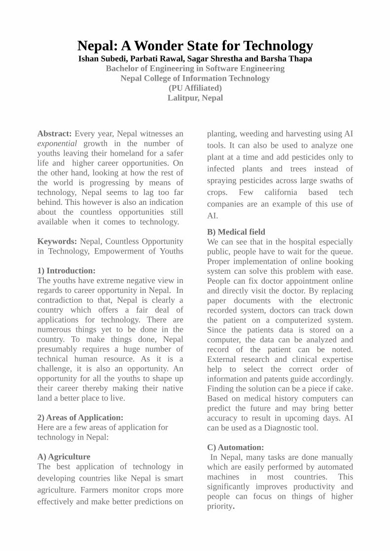
Nepal: A Wonder State for TechnologyIshan Subedi, Parbati Rawal, Sagar Shrestha and Barsha Thapa
Bachelor of Engineering in Software EngineeringNepal College of Information Technology
(PU Affiliated)Lalitpur, Nepal
Abstract: Every year, Nepal witnesses anexponential growth in the number ofyouths leaving their homeland for a saferlife and higher career opportunities. Onthe other hand, looking at how the rest ofthe world is progressing by means oftechnology, Nepal seems to lag too farbehind. This however is also an indicationabout the countless opportunities stillavailable when it comes to technology.
Keywords: Nepal, Countless Opportunityin Technology, Empowerment of Youths
1) Introduction: The youths have extreme negative view inregards to career opportunity in Nepal. Incontradiction to that, Nepal is clearly acountry which offers a fair deal ofapplications for technology. There arenumerous things yet to be done in thecountry. To make things done, Nepalpresumably requires a huge number oftechnical human resource. As it is achallenge, it is also an opportunity. Anopportunity for all the youths to shape uptheir career thereby making their nativeland a better place to live.
2) Areas of Application:Here are a few areas of application for technology in Nepal:
A) AgricultureThe best application of technology indeveloping countries like Nepal is smartagriculture. Farmers monitor crops moreeffectively and make better predictions on
planting, weeding and harvesting using AItools. It can also be used to analyze oneplant at a time and add pesticides only toinfected plants and trees instead ofspraying pesticides across large swaths ofcrops. Few california based techcompanies are an example of this use ofAI.
B) Medical fieldWe can see that in the hospital especiallypublic, people have to wait for the queue.Proper implementation of online bookingsystem can solve this problem with ease.People can fix doctor appointment onlineand directly visit the doctor. By replacingpaper documents with the electronicrecorded system, doctors can track downthe patient on a computerized system.Since the patients data is stored on acomputer, the data can be analyzed andrecord of the patient can be noted.External research and clinical expertisehelp to select the correct order ofinformation and patents guide accordingly.Finding the solution can be a piece if cake.Based on medical history computers canpredict the future and may bring betteraccuracy to result in upcoming days. AIcan be used as a Diagnostic tool.
C) Automation: In Nepal, many tasks are done manuallywhich are easily performed by automatedmachines in most countries. Thissignificantly improves productivity andpeople can focus on things of higherpriority.
D) TourismEverything for tour and traveling isavailable on a website. By this applicationpeople can decide variables likedestination, cost and time. For this, ifthere is conversational application it willbe more effective. And also Chabot, NLPcan reduced complexity. Face Recognitiontechnique can be used so that travelers canseemly move through airports,immigration customs and board aircraftwithout the need of having traveldocuments. There are social media listingtools, by listening to people interest itdisplay co-relates travel journey,awesome! By analyzing previous datafuture of travel and tourism of Nepal canbe made more effective and awesome.
3) Problems:The main problem is clearly lack ofskilled human resource. There’s a hugegap in terms of knowledge and skillsbetween fresh university graduates and thereal tech industry. In addition to that, lawsand policies have also proven to bediscouraging youths trying to dosomething innovative at certain times.Even registering a company is tedious andfrustrating job which in the most countriesis a single window job. Carrying out legaland governmental procedures tends to be ahuge barrier between aspiring youths andtheir dreams.
4) Conclusion: Nepal is evidently a bare state. Lots ofchallenges and with the challenges, lots ofopportunities exists. Innovation can startfrom anywhere. All we required is theright mindset and the passion to make ithappen.
5) Reference:
1. (Abhishek Chaudhary, June 12 ,2018)https://www.financialexpress.com/opinion/artificial-intelligence-a-smarter-way-to-build-smart-cities/1202358/
2. Nepal profile( ,pp.89-126.)http://shodhganga.inflibnet.ac.in/bitstream/10603/59251/10/10_chapter%203.pdf
3. Number of Nepali youth leavingfor foreign job destinations on therise ,(December 10,2018)https://thehimalayantimes.com/kathmandu/number-of-nepali-youths-leaving-for-foreign-job-destinations-on-the-rise
4. (AI For Humanity: Using AI ToMake A Positive Impact InDeveloping Countries, SameerMaskey, August 23 ,2018)https://www.forbes.com/sites/forbestechcouncil/2018/08/23/ai-for-humanity-using-ai-to-make-a-positive-impact-in-developing-countries-2/

Super-resolution: An Overview and its Modern
Application
S. Baral, B. Piryani
Department of Computer Engineering
Nepal College of Information Technology (NCIT)
Pokhara University
Lalitpur, Nepal
[email protected], [email protected]
Y. Maharjan
Department of Computer Science
Nepal College of Information Technology (NCIT)
Pokhara University
Lalitpur, Nepal
Abstract— The objective of super-resolution is to reconstruct a
high-resolution (HR) image from a low-resolution (LR) input
image. Super-resolution technique has been there for quite some
time and has received a lot of attention recently in the research
field. In this paper, we aim to provide an overview of super-
resolution and its different techniques used for reconstructing a
high-resolution image. The paper also discusses various
applications of super-resolution that impact our daily life.
Keywords: Super-resolution, image reconstruction, applications.
I. INTRODUCTION
In this world of digitization, most of the electronic image applications require high-resolution images or videos for image processing and analysis. Resolution describes the details of an image, high-resolution image capture more detailed image. Resolution enhancement is desired for two principal application areas: Pictorial enhancements for the human interaction and representation for the machine perception.
The classification of SR can be done in two families, i.e. single-frame based on the input LR (low resolution) and multi-frame based on the input LR. Similarly, about the resolution, we have many types, pixel resolution, spatial resolution, spectral resolution, temporal resolution, and radiometric resolution.
Here our primary focus will be on spatial resolution. Spatial resolution is defined as the pixel density of an image and can be calculated as pixels per unit area. (Pixels are the small elements which make a digital image).
Today, Charge-coupled devices (CCD) or a Complementary metal-oxide-semiconductor (CMOS) are the image sensors which are more likely to be used[1]. For achieving HR (high resolution) image one of the solutions is to be able to develop more advanced optical devices. To determine the spatial resolution of the image to be captured directly depends upon the sensor sizes or the number of sensor element per unit area. CCD or CMOS sensors are arranged in a two-dimensional array so that the two-dimensional image signal can be captured. For the possible higher spatial resolution there must be the higher density of sensors. If inadequate sensors are used then LR with blocky effects is obtained it is due to the aliasing from low spatial sampling frequency. To increase the spatial resolution one way can be
reducing the sensor size which will increase the sensor density. This causes the amount of light incident on the sensor to decrease which causes shot noise[2].
The spatial resolution is limited with the types of image sensors. Also due to the image details are bounded by the optics, i.e. (high-frequency bands), sensor point spread function (PSF) associated with lens causes blurring, lens aberration effects, aperture diffractions and optical blurring due to the motion. So, the hardware component for imaging and optics are costly and impractical in real case scenario: example, the camera used in CCTV and mobile devices.
SR is a technique which constructs a high-resolution image using several LR images despite using a low-resolution camera. The basic concept can be portrayed as combining the non-redundant information contained in the LR frame for the generation of HR image. In 1964, Harris introduced the theorems for solving the diffraction problem in the optical system. This can be referred as the theoretical foundation of SR problem. After two decades, Tsai and Huang proposed an idea to improve the spatial resolution of Landsat TM (Landsat thematic mapper) images. Since then various other research has been carried out. At the beginning, most of the methods were focused on the frequency domain. Due to more computational efficiency and simple theoretical basis, the frequency domain algorithms were popular. However, sensitivity to model errors and difficulty in handling more complicated motion models this algorithm is prevented from further development.
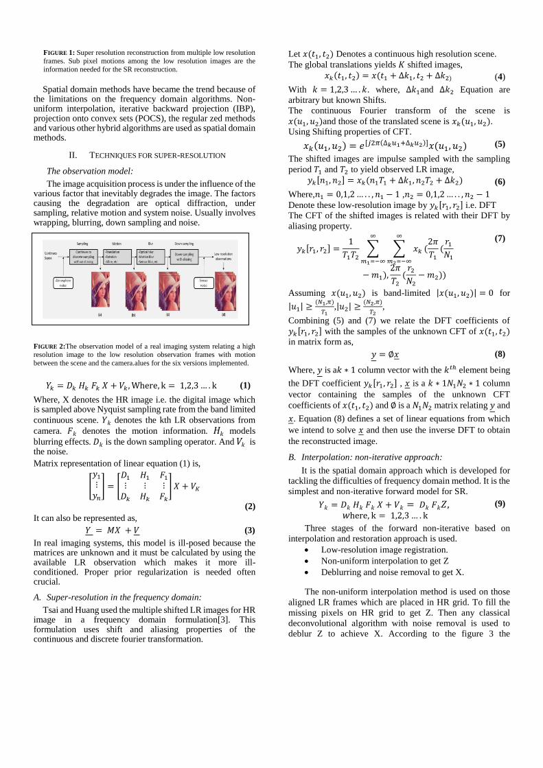
FIGURE 1: Super resolution reconstruction from multiple low resolution
frames. Sub pixel motions among the low resolution images are the information needed for the SR reconstruction.
Spatial domain methods have became the trend because of the limitations on the frequency domain algorithms. Non-uniform interpolation, iterative backward projection (IBP), projection onto convex sets (POCS), the regular zed methods and various other hybrid algorithms are used as spatial domain methods.
II. TECHNIQUES FOR SUPER-RESOLUTION
The observation model:
The image acquisition process is under the influence of the various factor that inevitably degrades the image. The factors causing the degradation are optical diffraction, under sampling, relative motion and system noise. Usually involves wrapping, blurring, down sampling and noise.
FIGURE 2:The observation model of a real imaging system relating a high resolution image to the low resolution observation frames with motion
between the scene and the camera.alues for the six versions implemented.
𝑌𝑘 = 𝐷𝑘 𝐻𝑘 𝐹𝑘 𝑋 + 𝑉𝑘 , Where, k = 1,2,3 … . k (1)
Where, X denotes the HR image i.e. the digital image which is sampled above Nyquist sampling rate from the band limited
continuous scene. 𝑌𝑘 denotes the kth LR observations from
camera. 𝐹𝑘 denotes the motion information. 𝐻𝑘 models
blurring effects. 𝐷𝑘 is the down sampling operator. And 𝑉𝑘 is the noise.
Matrix representation of linear equation (1) is,
[
𝑦1
⋮𝑦𝑛
] = [𝐷1 𝐻1 𝐹1
⋮ ⋮ ⋮𝐷𝑘 𝐻𝑘 𝐹𝑘
] 𝑋 + 𝑉𝐾
(2)
It can also be represented as,
𝑌 = 𝑀𝑋 + 𝑉 (3)
In real imaging systems, this model is ill-posed because the matrices are unknown and it must be calculated by using the available LR observation which makes it more ill-conditioned. Proper prior regularization is needed often crucial.
A. Super-resolution in the frequency domain:
Tsai and Huang used the multiple shifted LR images for HR image in a frequency domain formulation[3]. This formulation uses shift and aliasing properties of the continuous and discrete fourier transformation.
Let 𝑥(𝑡1, 𝑡2) Denotes a continuous high resolution scene.
The global translations yields 𝐾 shifted images,
𝑥𝑘(𝑡1, 𝑡2) = 𝑥(𝑡1 + ∆𝑘1, 𝑡2 + ∆𝑘2) (4)
With 𝑘 = 1,2,3 … . 𝑘. where, ∆𝑘1and ∆𝑘2 Equation are
arbitrary but known Shifts.
The continuous Fourier transform of the scene is
𝑥(𝑢1, 𝑢2)and those of the translated scene is 𝑥𝑘(𝑢1, 𝑢2).
Using Shifting properties of CFT.
𝑥𝑘(𝑢1, 𝑢2) = 𝑒[𝑗2𝜋(∆𝑘𝑢1+∆𝑘𝑢2)]𝑥(𝑢1, 𝑢2) (5)
The shifted images are impulse sampled with the sampling
period 𝑇1 and 𝑇2 to yield observed LR image,
𝑦𝑘[𝑛1, 𝑛2] = 𝑥𝑘(𝑛1𝑇1 + ∆𝑘1, 𝑛2𝑇2 + ∆𝑘2) (6)
Where,𝑛1 = 0,1,2 … . . , 𝑛1 − 1 ,𝑛2 = 0,1,2 … . . , 𝑛2 − 1
Denote these low-resolution image by 𝑦𝑘[𝑟1, 𝑟2] i.e. DFT
The CFT of the shifted images is related with their DFT by
aliasing property.
𝑦𝑘[𝑟1, 𝑟2] =1
𝑇1𝑇2
∑ ∑ 𝑥𝑘
∞
𝑚2=−∞
(2𝜋
𝑇1
(𝑟1
𝑁1
∞
𝑚1=−∞
− 𝑚1),2𝜋
𝑇2
(𝑟2
𝑁2
− 𝑚2))
(7)
Assuming 𝑥(𝑢1, 𝑢2) is band-limited |𝑥(𝑢1, 𝑢2)| = 0 for
|𝑢1| ≥(𝑁1,𝜋)
𝑇1,|𝑢2| ≥
(𝑁2,𝜋)
𝑇2,
Combining (5) and (7) we relate the DFT coefficients of
𝑦𝑘[𝑟1, 𝑟2] with the samples of the unknown CFT of 𝑥(𝑡1, 𝑡2)
in matrix form as,
𝑦 = ∅𝑥 (8)
Where, 𝑦 is a𝑘 ∗ 1 column vector with the 𝑘𝑡ℎ element being
the DFT coefficient 𝑦𝑘[𝑟1, 𝑟2] , 𝑥 is a 𝑘 ∗ 1𝑁1𝑁2 ∗ 1 column
vector containing the samples of the unknown CFT
coefficients of 𝑥(𝑡1, 𝑡2) and ∅ is a 𝑁1𝑁2 matrix relating 𝑦 and
𝑥. Equation (8) defines a set of linear equations from which
we intend to solve 𝑥 and then use the inverse DFT to obtain
the reconstructed image.
B. Interpolation: non-iterative approach:
It is the spatial domain approach which is developed for
tackling the difficulties of frequency domain method. It is the
simplest and non-iterative forward model for SR.
𝑌𝑘 = 𝐷𝑘 𝐻𝑘 𝐹𝑘 𝑋 + 𝑉𝑘 = 𝐷𝑘 𝐹𝑘𝑍, 𝑤here, k = 1,2,3 … . k
(9)
Three stages of the forward non-iterative based on
interpolation and restoration approach is used.
Low-resolution image registration.
Non-uniform interpolation to get Z
Deblurring and noise removal to get X.
The non-uniform interpolation method is used on those
aligned LR frames which are placed in HR grid. To fill the
missing pixels on HR grid to get Z. Then any classical
deconvolutional algorithm with noise removal is used to
deblur Z to achieve X. According to the figure 3 the

alignment using some image registration algorithm to sub-
pixel accuracy is done for LR frames.
FIGURE 3: The interpolation SR approach based on alignment and post
processing of deblurring.
Various techniques using interpolation are used for the
restoration of the image which are intuitive, simple and
computationally efficient using simple observational model.
But ideal estimation is not guaranteed since the registration
error can easily be generated to the later processing. Also, it
is meaningless without the noise and blurring effect
consideration. Interpolation based approaches also need
some correction to reduce aliasing if without using an HR
image initially as proper regularization.
C. Statistical Approach:
This approach randomly defined towards the optimal
reconstruction of SR. Both the HR image and motion of LR
inputs are random variables.
Let 𝑚(𝑣, ℎ), where 𝑣 is the motion vector(usually stands
for additive noise i.e.,zero-mean and white Gaussian random
vecor) and ℎ is the blurring kernel. This matrix is called as a
degradation matrix
Using Bayesian framework for SR reconstruction.
𝑋 = 𝑎𝑟𝑔 max𝑥
Pr (𝑋 𝑦⁄ ) (10)
𝑋 = 𝑎𝑟𝑔 max𝑥
∫ 𝑃𝑟(𝑋, 𝑚(𝑣, ℎ) 𝑦)⁄ℎ
𝑣
𝑑𝑣
(11)
𝑋 = max𝑥
∫𝑃𝑟(𝑦 𝑋, 𝑚(𝑣, ℎ))𝑃𝑟(𝑋, 𝑚(𝑣, ℎ))⁄
Pr (𝑦)
ℎ
𝑣
𝑑𝑣
(12)
𝑋 =
𝑎𝑟𝑔 max𝑥
∫ 𝑃𝑟(ℎ
𝑣(𝑦 𝑋, 𝑚(𝑣, ℎ))𝑃𝑟(𝑋)Pr (𝑚(𝑣, ℎ))⁄ 𝑑𝑣
(13)
Here, 𝑥 and 𝑚(𝑣, ℎ) are statistically independent.
𝑃𝑟(𝑦 𝑋, 𝑚(𝑣, ℎ))⁄ , is the data likelihood. Pr(𝑋), is the prior
term on the desired HD image. Pr(𝑚(𝑣, ℎ)), is the prior term
on the motion estimation
𝑃𝑟(𝑦 𝑋, 𝑚(𝑣, ℎ))⁄ 𝛼𝑒{−
1
2𝜎2‖𝑦−𝑚(𝑣,ℎ)𝑋‖
2}
(14)
Pr (𝑋)is defined using Gibbs distribution in the exponential
form
Pr(𝑋) =1
𝑍𝑒{−𝛼𝐴(𝑋)}
(15)
Here, 𝐴(𝑋) is a non-negative potential function. 𝑍 is a
normalization factor. The Bayesian formulation due to the
integration over motion is tedious to evaluate.
If 𝑚(𝑣, ℎ) is calculated before and expressed as 𝑚 then,
𝑋 = arg max𝑥
Pr ( 𝑦 𝑥, 𝑚⁄ )Pr (𝑋) (16)
𝑋 = arg min𝑥
{‖𝑦 − 𝑚𝑥‖2
+ 𝜆𝐴(𝑋)} (17)
Where, the above equation is Maximum a posterior
formulation, 𝑀is assumed to be known, 𝜆 absorbs the
variance of thr noise and α in equation (15).
D. Maximum a posteriori:
MAP approach is used for many models of SR
reconstruction. The technique is different in assumption of
observation model and prior team 𝑝𝑟(𝑥). The most
commonly used are listed below.
a. Guassian MRF (Gaussian markov random field)
𝐴(𝑋) = 𝑋𝑇 𝑄 𝑋 (18)
Where, 𝑄 is a symmetric positive matrix which contains the
spatial relation among the adjacent pixel in the image its off-
diagonal elements, 𝑄 can also be referred as 𝜏𝑇𝜏.
Here, 𝜏 acts as a first or second derivative operator on the
image 𝑋 and is called Tiknov matrix.
According to tiknov regularization,
Log likelihood of the prior is,
𝐿𝑜𝑔 𝑃 (𝑋) 𝛼 ‖𝜏𝑋‖2 (19)
Even the advantages are very significant but due to the overly
smooth results sharp edges cannot recovered.
b. Huber MRF
Modeling of image gradients with a distribution with
heavier tails is the main advantage over the guassian MRF.
Gibbs potential are determined but the Huber function.

𝜌(𝑎) = {𝑎2, |𝑎| ≤ 𝛼
2𝛼|𝑎| − 𝛼2, 𝑜𝑡ℎ𝑒𝑟𝑤𝑖𝑠𝑒
(20)
Where, 𝑎 is the first derivative of the image using this kind
of prior preserve edges and also produce smoothness.
c. Total variation
Total variation (TV) is very much useful for the image
denoising and deblurring. Typically use as a gradient
penalty funchtion.
𝐴(𝑋) = ‖∇𝑋‖1 (21)
Where, ∇ is a gradient operator using laplacian operator.
E. Joint MAP restoration:
The two parts of SR construction can be: LR registration and
HR estimation. The method above treat these process as a two
different processes. The working was to registration of first
and estimation of second. In joint MAP the above equation
can be extended where PSF (point spread function) and the
motion is included.
{ X, v, h} = arg max
𝑥,𝑣,ℎPr ( 𝑦 𝑋, 𝑚(𝑣, ℎ)⁄ )Pr (𝑋)Pr (𝑚(𝑣, ℎ))
= arg max𝑥,𝑣,ℎ
−log [Pr ( 𝑦 𝑋, 𝑚(𝑣, ℎ)⁄ )] − log [Pr (𝑋)]
− log [Pr (𝑚(𝑣, ℎ))]
(22)
Tom et. Al. further divided the process into three sub
problems, registration, restoration and interpolation. This
improves the estimation more accurately than using two
processes.
F. The Bayesian framework:
Unlike the MAP estimator, the posterior distribution is
calculated instead manual setting of specific value of the
parameters. Bayesian method calculates whole posterior
distribution unlike in ML or MAP.
P(X, m(v, h)|Y)
= Pr(𝑌 𝑋, 𝑚(𝑣, ℎ)⁄ ) Pr(𝑋) Pr(𝑚(𝑣, ℎ)) /Pr (Y) (23)
Where, 𝑃(𝑌) is generally ignored in MAP estimators. It is
independent of the unknown variable and it cannot be
computed so approximation must be done for reconstruction.
G. Example based super-resolution:
The methods above were based on aggregating multiple
frames which have complementary spatial information. If
only a single LR image is observed then the measurements
are insufficient. A recent uprising process for the
regularization of the ill-posed SR is example based. To
overcome the inadequate measurement limits using examples
which develops the priors by sampling from other images.
One of the approaches of example-based is by using the
example directly. This approach is proposed by Freeman et.
al. where two set of training patches are maintained,
{𝑋𝑖}𝑖=1𝑛 , 𝑠𝑎𝑚𝑝𝑙𝑒𝑑 𝑓𝑟𝑜𝑚 ℎ𝑖𝑔ℎ 𝑟𝑒𝑠𝑜𝑙𝑢𝑡𝑖𝑜𝑛 𝑖 (24)
{𝑌𝑖}𝑖=1𝑛 , 𝑠𝑎𝑚𝑝𝑙𝑒𝑑 𝑓𝑟𝑜𝑚 𝑙𝑜𝑤 𝑟𝑒𝑠𝑜𝑙𝑢𝑡𝑖𝑜𝑛 𝑖𝑚𝑎𝑔𝑒 (25)
The observation model,
𝑌𝑖 = 𝐷 𝐻 𝑋𝑖 + 𝑉𝑘 (26)
Using the MRF model as shown in figure the co-
occurrence of HR and LR is applied to the target image for
HR prediction in a patch-based fashion.
The parameter of the observation model should be known
as prior; the training sets are tightly coupled with the image
targeted. The size of the patch must be a proper choice. Due
to variation path size if it is too small, then co-occurrence
priors to weak for prediction and if it is too large, there may
be a need of huge training set.
III. APPLICATION
After going through the methods above, we will discuss the specific application of SR. The uses of SR in our daily life with which we can benefits in various ways are the basic concern.
A. Video information enhancement
The SR technique can be used for the conversion of LR video or image into HD. Hitachi Ltd. Successfully used the conversion of standard definition TV into high definition television. Moreover, Apple Inc. used SR based optical image stabilization and also applied for a patent on the concept. This technology will be used in our phones, computers, and tablets in the near future.
B. Medical application
SR has a very significant role in the medical field. The good
quality of the medical image can be generated which will
have a profound impact on the ease of diagnosis. As in CT
scan, MRI and other medical procedures image enhancement
are needed. The geometric deformation on the image can be
corrected. It is more desirable to detect the disease in early
stage. This application of SR will give a better and clear
understandability of the image we try to achieve in medical
diagnosis.

C. Surveillance
Traffic surveillance and security cameras which have the digital video recording can also be improved using SR. due to many weather condition and different motion complexity it is still a challenge.
D. Remote sensing (Earth-observation)
Initially, the research about the SR was done for the betterment of the image quality in Landsat remote sensing image. More than decodes the technique has been developing for remote sensing image. Some of the few relevant examples are SPOT-5 which can reach 2.5m through the SR of two 5m images by shifting a double CCD array by half a sampling interval. Moreover, Landsat, CBERS and worldview 2 also provide the possibility of SR. many researchers have also tried to use the example-based methods. Recently 24 small satellites capturing and delivering real-time “videos” using a sub-meter resolution using SR which has been done by Skybox.
E. Astronomical observation
Many astronomers are exploring the outer space, and for those researchers, SR can be a beneficial utility. By enhancing and improving the quality of astronomical image, the exploration can obtain more depth. Lunar exploration program and the Mars Odyssey mission are the SR example of Chinese Chang’ E-1 lunar images. Moreover, Hughes and Ramsey used (THEMIS), i.e. thermal emission system to generate the enhanced thermal infrared image of surface mars.
F. Biometric
The recognition of faces, fingerprints and iris images where the enhancement of resolution is very important factor for the proper biometric information. The resolution is the crucial
factor with which the detection process can be made efficient. The details of images like the shape and structural texture should be enhanced for the recognition ability. A very fast and accurate biometric information can be generated if the resolution becomes clear and distinguishable.
IV. CONCLUSION
In this paper, we have discussed about the Super-resolution technique which is one of the most popular approach for reconstructing High-resolution image from Low-resolution image in spite of low resolution camera. We have also looked at various methods of super-resolution and their various applications in the daily life.
.
REFERENCES
[1] L. Yue, H. Shen, J. Li, Q. Yuan, H. Zhang, and L. Zhang, “Image super-resolution: The techniques, applications, and future,” Signal Processing, vol. 128, pp. 389–408, Nov. 2016.
[2] B. Shi, H. Zhao, M. Ben-Ezra, S.-K. Yeung, C. Fernandez-Cull, R. H. Shepard, C. Barsi, and R. Raskar, “Sub-pixel Layout for Super-Resolution with Images in the Octic Group,” Lecture Notes in Computer Science, pp. 250–264, 2014.
[3] R. Y. Tsai and T. S. Huang. “Multipleframe image restoration and registration” Advances in Computer Vision and Image Processing, pages 317{339. Greenwich, CT: JAI Press Inc., 1984.
[4] J. Yang, T. Huang, “Image super-resolution: historical overview and future challenges.
[5] W. T. Freeman, T. R. Jones, and E. C. Pasztor, “Example-based super-resolution,” IEEE Computer Graphics and Applications, vol. 22, no. 2, pp. 56-65, 2002.
[6] J. Salvador, “ A Taxonomy of Example-Based Super Resolution,” Example-Based Super Resolution, pp. 15-29, 2017.
[7] D. Capel, “ Super-resolution: Maximum Likelihood and Related Approaches”, Image Mosaicing and super-resolution, pp. 81-136, 2004.
[8] D. Capel, “ Super-resolution using Bayesion Priors”, Image Mosaicing and super-resolution, pp. 137-168, 2004.
[9] “Research on Image Super-Resolution,” Motion-Free Super-Resolution, pp. 15-31.
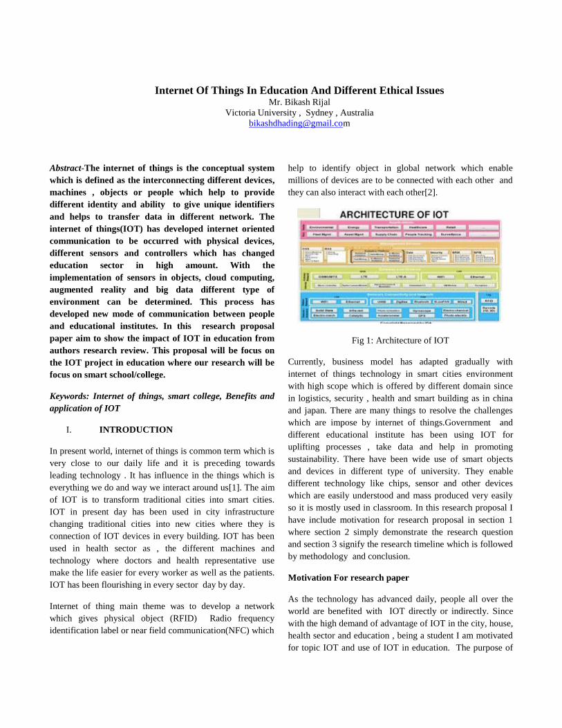
Internet Of Things In Education And Different Ethical Issues Mr. Bikash Rijal
Victoria University , Sydney , Australia
Abstract-The internet of things is the conceptual system
which is defined as the interconnecting different devices,
machines , objects or people which help to provide
different identity and ability to give unique identifiers
and helps to transfer data in different network. The
internet of things(IOT) has developed internet oriented
communication to be occurred with physical devices,
different sensors and controllers which has changed
education sector in high amount. With the
implementation of sensors in objects, cloud computing,
augmented reality and big data different type of
environment can be determined. This process has
developed new mode of communication between people
and educational institutes. In this research proposal
paper aim to show the impact of IOT in education from
authors research review. This proposal will be focus on
the IOT project in education where our research will be
focus on smart school/college.
Keywords: Internet of things, smart college, Benefits and
application of IOT
I. INTRODUCTION
In present world, internet of things is common term which is
very close to our daily life and it is preceding towards
leading technology . It has influence in the things which is
everything we do and way we interact around us[1]. The aim
of IOT is to transform traditional cities into smart cities.
IOT in present day has been used in city infrastructure
changing traditional cities into new cities where they is
connection of IOT devices in every building. IOT has been
used in health sector as , the different machines and
technology where doctors and health representative use
make the life easier for every worker as well as the patients.
IOT has been flourishing in every sector day by day.
Internet of thing main theme was to develop a network
which gives physical object (RFID) Radio frequency
identification label or near field communication(NFC) which
help to identify object in global network which enable
millions of devices are to be connected with each other and
they can also interact with each other[2].
Fig 1: Architecture of IOT
Currently, business model has adapted gradually with
internet of things technology in smart cities environment
with high scope which is offered by different domain since
in logistics, security , health and smart building as in china
and japan. There are many things to resolve the challenges
which are impose by internet of things.Government and
different educational institute has been using IOT for
uplifting processes , take data and help in promoting
sustainability. There have been wide use of smart objects
and devices in different type of university. They enable
different technology like chips, sensor and other devices
which are easily understood and mass produced very easily
so it is mostly used in classroom. In this research proposal I
have include motivation for research proposal in section 1
where section 2 simply demonstrate the research question
and section 3 signify the research timeline which is followed
by methodology and conclusion.
Motivation For research paper
As the technology has advanced daily, people all over the
world are benefited with IOT directly or indirectly. Since
with the high demand of advantage of IOT in the city, house,
health sector and education , being a student I am motivated
for topic IOT and use of IOT in education. The purpose of

1
this conference paper is to give description of IOT where
benefit of IOT in education, difficulties while implementing
IOT in Education, demerits of IOT in education and how
present world is booming with IOT are described. I have
also proposed the boundaries of my conference paper where
I will focus on overview of IOT in present world, concept of
smart school and university along with benefit of IOT to
education mitigating its demerits. The use of IOT helps to
transforms static classrooms and education environment to
digital classroom which can be easily connected to smart
devices[3] . This techniques of IOT in education is very
useful for disability student or teachers where they can
extract materials online and can see their classroom
activities through home and can know how all the system are
working from anywhere at anytime.
II. RESEARCH QUESTION
The objectives of the research is to know about the influence
of IOT in education. In present world IOT is used in
different places for benefit of the people. With the use of
IOT in education student will lack creativity and they can be
lazy, there may be private issues. The main research
question are finding benefit of IOT in education, difficulties
while implementing IOT in education and how IOT is
booming in the present world.
III. PAPER DESCRIPTION
IOT is being popular day today with the advanced of the
internet, different devices, system and software are
interconnected with each other. People have become more
advanced. These integrated devices connected with internet
and generating and viewing how all the devices and system
are running in different places, institution is the today
reality. Individual can easily share all of the data , progress,
concepts , different simulation with each other from different
places. IOT has great influence in the home, city, health
sector , education with the use of IOT the physical devices
of these sectors are connected to each other which form
smart home, smart city , smart hospital along with smart
school and smart college. IOT also enables different services
with interconnection of information and communication
technology.
The implementation of IOT in education is in just starting
phase. The development of smallest wireless devices which
requires function and most of them are controlled by smart
phones gives benefit for student who are engaged in remote
controlling of devices.
The key objectives of this report are:-
1. To find the benefit of IOT in making school and
college into smart school and smart college
2. The difficulties and demerits of IOT in education
3. How IOT is booming in present context
From 2016 it is estimated that there are about 6.4 billion of
the devices which are connected with each other[4]. The
implication of IOT in education has been very beneficial to
the educational institutes where it makes student centred
approach in function which helps to find hear beat rate, brain
signals and it provides different notification , the sensor
connected devices helps to collect different data which
include physical and mental activity , heart beat rate, calories
consumption, stress level with the help of this school
administration can provide new nutrition schedule, reduce
stress causes which will be very useful for students. It helps
in improving educational institute securities. There have
been problem of kidnapping children from school, shooting
of children in school premises with gun, this will be in
control with the use of smart gadget when connected with
people where security is achieved with door gateway and
recognition software. The use of global digital security also
reduces maintenance cost.
Internet of things has major impact on todays education
system where it provides better path how to learn, along with
that it helps in tracking objects, students , staff and helps to
connect devices across school which brings safety to
institution[16]. It also help to track buses of school where
student can track the buses and they shouldn’t wait for long.
It also helps to ensure cashless environment and these things
are just beginning of IOT in education. IOT had higher
benefits it cannot be implemented everywhere, there are
some shortcoming of IOT in education such as security
issue, integration and low financing in different ways. There
may be problem in financing as IOT requires different
hardware and software where wearable devices like beacons,
wristband along with interactive board is costly and
integration of those devices with each other and software can
also malfunction. There is no single platform for IOT user
so it is difficult to integrate. Since IOT network is very big it
consist of different devices which connect many gadget and
device and it leads hacker to breach the security of devices
and find loop holes. This things can be mitigate by having
authentication tools and firewall only.
In this conference paper chapter 1 consists of introduction of
IOT whereas chapter 2 consists of the review of the 5
different papers and chapter 3 consist of the conclusion.

2
IV. EFFECT ON EDUCATION BUSINESS MODEL
There had been research going on for IOT in education. In
this report 1 writer has proposed smart classroom as an
intelligent environment which is collaborate with different
types of hardware and software. There are uses of different
smart object which are used in university. This paper mainly
focus with effects of IOT in education where it mainly give
special concentration on use of IOT in higher education,
how energy management is done in campuses and effective
campus security along with classroom access control where
it include systematic student healthcare and describe how
teaching can be enhanced[6] . Moreover, education business
model which is based on Canvas Business model approach is
described in suitable way.
This report describes seven categories where technical
education can be derived which are visualisation, learning,
social media , Digital consumer, technology . The concept of
smart classroom is special environment where it contains
video projector, camera , sensor and face recognition and
different entities which are fitted to know student progress
along with performance and achievement. It has described
IOT in education as personalized and medium for effective
interaction with student. Report describe how student can
solve their problem how they are suffering by just sending
alert to administration. IOT is used in classroom for
improvement of teaching and learning where remote
presence of students, optimizing classroom. IOT not only
help student but also to administration where they can
understand student and their needs along with student health,
safety and they can connect everything on campus
management . This paper gives idea how IOT can benefit
higher education and it describe how future IOT in education
should be.
IOT business model
This paper describe education business model where
business model is a tool which consists of object s concept
and close relationship with objective to express business
logic in firm. It defines 9 sections where customer segment
focus with people whom organization serves. In any
organization customer are student, parents and government
value proposition, customer relationship, channel key
activities , key resources , key partners cost structure ,
revenue streams are new framework used in education
business model[5].
Benefits
There have been benefits achieved such as:-
Adding new value proposition
1. The addition of value proposition in education
business model with active involvement at IOT
in education.
a) It will reduce cost by automating operation
where energy can be able to access real time
energy consumption.
b) It helps in customization of curriculum.
c) There will be easier for access of leaning
resources.
d) Collaboration can be done easily between
stake- holder.
e) Helps in increasing virtualization and
personalization.
f) Real time interaction becomes easier.
g) Constant data collection and analysis possible.
h) People and environment database can be
formed.
i) It helps to save time where we can access
different part with the help of RFID or NFC.
Problem tackled
The problem tackled in this report is as
follows.
a) It has focused on higher education but the
infrastructure cost seems higher.
b) It has increased technology and
management cost.
CONCLUSION
This research explains mainly how internet of things can
enhance smart campuses and classroom where they
categorized application of IOT into different segments and
this campus energy management, access control system ,
ecosystem monitoring and canvas model show IOT has
played big role on education system which directly reduce
cost along with comfort and collaboration and make
relationship between channel and customer by forming
virtual and personalized relation.
V. A SURVEY ON ROLE OF IOT IN
EDUCATION
The paper “ A survey on role of Internet of things in
Education “ defines IOT as a growing network where variety
of connected things are rewind. The use of IOT in education
helps in improvement of teaching process and educational
sector . This paper mainly describe usefulness and
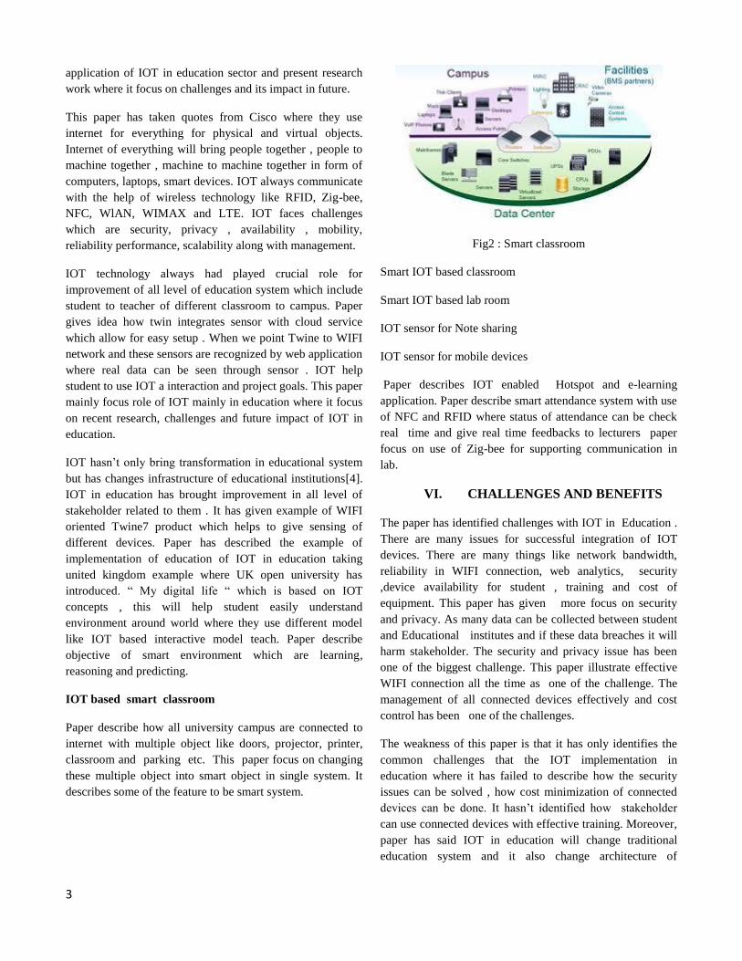
3
application of IOT in education sector and present research
work where it focus on challenges and its impact in future.
This paper has taken quotes from Cisco where they use
internet for everything for physical and virtual objects.
Internet of everything will bring people together , people to
machine together , machine to machine together in form of
computers, laptops, smart devices. IOT always communicate
with the help of wireless technology like RFID, Zig-bee,
NFC, WlAN, WIMAX and LTE. IOT faces challenges
which are security, privacy , availability , mobility,
reliability performance, scalability along with management.
IOT technology always had played crucial role for
improvement of all level of education system which include
student to teacher of different classroom to campus. Paper
gives idea how twin integrates sensor with cloud service
which allow for easy setup . When we point Twine to WIFI
network and these sensors are recognized by web application
where real data can be seen through sensor . IOT help
student to use IOT a interaction and project goals. This paper
mainly focus role of IOT mainly in education where it focus
on recent research, challenges and future impact of IOT in
education.
IOT hasn’t only bring transformation in educational system
but has changes infrastructure of educational institutions[4].
IOT in education has brought improvement in all level of
stakeholder related to them . It has given example of WIFI
oriented Twine7 product which helps to give sensing of
different devices. Paper has described the example of
implementation of education of IOT in education taking
united kingdom example where UK open university has
introduced. “ My digital life “ which is based on IOT
concepts , this will help student easily understand
environment around world where they use different model
like IOT based interactive model teach. Paper describe
objective of smart environment which are learning,
reasoning and predicting.
IOT based smart classroom
Paper describe how all university campus are connected to
internet with multiple object like doors, projector, printer,
classroom and parking etc. This paper focus on changing
these multiple object into smart object in single system. It
describes some of the feature to be smart system.
Fig2 : Smart classroom
Smart IOT based classroom
Smart IOT based lab room
IOT sensor for Note sharing
IOT sensor for mobile devices
Paper describes IOT enabled Hotspot and e-learning
application. Paper describe smart attendance system with use
of NFC and RFID where status of attendance can be check
real time and give real time feedbacks to lecturers paper
focus on use of Zig-bee for supporting communication in
lab.
VI. CHALLENGES AND BENEFITS
The paper has identified challenges with IOT in Education .
There are many issues for successful integration of IOT
devices. There are many things like network bandwidth,
reliability in WIFI connection, web analytics, security
,device availability for student , training and cost of
equipment. This paper has given more focus on security
and privacy. As many data can be collected between student
and Educational institutes and if these data breaches it will
harm stakeholder. The security and privacy issue has been
one of the biggest challenge. This paper illustrate effective
WIFI connection all the time as one of the challenge. The
management of all connected devices effectively and cost
control has been one of the challenges.
The weakness of this paper is that it has only identifies the
common challenges that the IOT implementation in
education where it has failed to describe how the security
issues can be solved , how cost minimization of connected
devices can be done. It hasn’t identified how stakeholder
can use connected devices with effective training. Moreover,
paper has said IOT in education will change traditional
education system and it also change architecture of
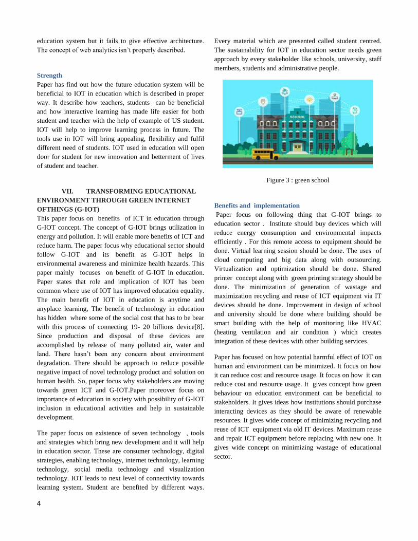
4
education system but it fails to give effective architecture.
The concept of web analytics isn’t properly described.
Strength
Paper has find out how the future education system will be
beneficial to IOT in education which is described in proper
way. It describe how teachers, students can be beneficial
and how interactive learning has made life easier for both
student and teacher with the help of example of US student.
IOT will help to improve learning process in future. The
tools use in IOT will bring appealing, flexibility and fulfil
different need of students. IOT used in education will open
door for student for new innovation and betterment of lives
of student and teacher.
VII. TRANSFORMING EDUCATIONAL
ENVIRONMENT THROUGH GREEN INTERNET
OFTHINGS (G-IOT)
This paper focus on benefits of ICT in education through
G-IOT concept. The concept of G-IOT brings utilization in
energy and pollution. It will enable more benefits of ICT and
reduce harm. The paper focus why educational sector should
follow G-IOT and its benefit as G-IOT helps in
environmental awareness and minimize health hazards. This
paper mainly focuses on benefit of G-IOT in education.
Paper states that role and implication of IOT has been
common where use of IOT has improved education equality.
The main benefit of IOT in education is anytime and
anyplace learning, The benefit of technology in education
has hidden where some of the social cost that has to be bear
with this process of connecting 19- 20 billions device[8].
Since production and disposal of these devices are
accomplished by release of many polluted air, water and
land. There hasn’t been any concern about environment
degradation. There should be approach to reduce possible
negative impact of novel technology product and solution on
human health. So, paper focus why stakeholders are moving
towards green ICT and G-IOT.Paper moreover focus on
importance of education in society with possibility of G-IOT
inclusion in educational activities and help in sustainable
development.
The paper focus on existence of seven technology , tools
and strategies which bring new development and it will help
in education sector. These are consumer technology, digital
strategies, enabling technology, internet technology, learning
technology, social media technology and visualization
technology. IOT leads to next level of connectivity towards
learning system. Student are benefited by different ways.
Every material which are presented called student centred.
The sustainability for IOT in education sector needs green
approach by every stakeholder like schools, university, staff
members, students and administrative people.
Figure 3 : green school
Benefits and implementation
Paper focus on following thing that G-IOT brings to
education sector . Institute should buy devices which will
reduce energy consumption and environmental impacts
efficiently . For this remote access to equipment should be
done. Virtual learning session should be done. The uses of
cloud computing and big data along with outsourcing.
Virtualization and optimization should be done. Shared
printer concept along with green printing strategy should be
done. The minimization of generation of wastage and
maximization recycling and reuse of ICT equipment via IT
devices should be done. Improvement in design of school
and university should be done where building should be
smart building with the help of monitoring like HVAC
(heating ventilation and air condition ) which creates
integration of these devices with other building services.
Paper has focused on how potential harmful effect of IOT on
human and environment can be minimized. It focus on how
it can reduce cost and resource usage. It focus on how it can
reduce cost and resource usage. It gives concept how green
behaviour on education environment can be beneficial to
stakeholders. It gives ideas how institutions should purchase
interacting devices as they should be aware of renewable
resources. It gives wide concept of minimizing recycling and
reuse of ICT equipment via old IT devices. Maximum reuse
and repair ICT equipment before replacing with new one. It
gives wide concept on minimizing wastage of educational
sector.

5
Weakness
Paper fail to describe how seven categories like customer
technology , Digital strategies , Enabling technology ,
Learning technology and social media technology
integration could help in making green IOT in education.
Paper focus on how old devices can be used and new eco
friendly devices should be purchased but fails to describe
architecture and production technique of eco friendly
devices.
VIII. INTERNET OF THINGS (IOT): AN
OVERVIEW
Paper focus on the emerging technology of Internet of
Things (IOT) provides promising benefits to individuals and
various organizations. With the advancements in smart
devices, wireless network, and other technologies, the field
of IOT is moving forward. However, along with the
promises, it has its challenges as well. This paper looks over
the benefits, challenges, and the security issues associated
with IOT.
Historical Background
IOT enables communications between person and object and
object and object[9]. The interconnection of various sensors,
RFID devices, and other objects creates a digital ecosystem.
According to Carlos Elena-Lenz, the main aspects of IOT
are Intelligence, connectivity, safety, energy, expressing, and
sensing where each characteristics can be traded off during
the design.
Technology and Platform of IOT
There are four main components of IOT networks: control
units, sensors, modules for communication and power
sources driven by the following features respectively: collect
and transmit data, run devices, get information and help in
communication. Sensor is the one that connects physical
world with the virtual world which collects data from
environment and convert them into digital data. Some of the
technologies assisting IOT includes, RFID (Radio Frequency
Identification), Bluetooth, Zig bee, Wi-Fi RF links, and
cellular networks.
Pervasiveness of IOT
Some societies are not feeling easy with the development of
the this technology fearing human functionalities like
replacement with machine and thus the fear of
unemployment.
Benefits of IOT
There are various advantages as well as challenges of this
emerging technology in various fields. They are discussed
below:
Health Sector: IOT can help monitor patients and identify
the signals with urgent attention. Patients also get relevant
information regarding their health.
Security: Vehicles and property can be monitored through
IOT. In cases of crashes, emergency call and rescue can be
delivered. Even kids could be monitored.
Business: Businesses can monitor their asset, production
process, consumers, and inventory control ultimately
improving their visibility of constant supply.
Education: In education, there are numerous benefits. Data
could be collected and analysed easily for researches.
Learning skills can be improved as it provides a new
approach to studying. Education can be more mobile with
this technology. The error that occur as a result of manual
handling can be reduced by this technology. This increases
efficiency. Students who cannot attend school for various
reasons can get distant learning and can participate
completely in a classroom activity. Special students can get
support from this technology as well.
Challenges of IOT:
Broadly, the challenges of I0T are categorized into three
categories: privacy, over reliance, and unemployment.
Privacy:
There is a big possibility of hackers hacking information
putting many individuals and companies at risk of
information exposure or leaking.
Over reliance: When the system collapses, over dependency
could result in a catastrophic event leading a failure of a
whole business.
Security Issues:
With the spread of IOT, cyber-attacks are likely to increase.
Various problems like unauthorized data access, sharing of
those data, privacy breach could be highly inevitable.
Strong security solutions are necessary to address this
problem. The system developed must be impregnable,
inaccessible to unauthorized users, and devices must be
6
controlled. Setting standards can help to address the security
issues to some extent.
IX. Conclusion:
IOT have the potential to bring a technological upliftment of
the human society and the development of this technology
depends on a number of other important fields, ranging from
nanotechnology to wireless sensors. With this technology,
real world can connect with a virtual world throughout the
world through various sensors and other technologies.
Strength: good overview of IOT. Good historical
information. Well Structured
Weakness: Not much information. Not detail information.
No examples.
Internet of Things (IOT): Education and Technology
IOT is “ not a single technology but it is combination of
various technology which work together in tandem[12].
This is the report which is made my Curtin university for its
vision for 2030 for the development of its campus as city of
innovation where it take Internet of things as its key features.
IOT mainly focus on its application in home, betterment to
education system. Paper suggest that the use of IOT in
education is in infancy level where there is little information
for student about the IOT. This reports mainly focus the case
of students who are disabled. The paper defines the concept
of smart campus where the purpose of I campus isn’t to
enhance interactivity in education but to create a campus
made of different intelligent computer system. These system
should understand individual context of student as well as
having an intelligent understanding of environments in
which they study.
Benefits and risk
This report finds the risk and benefits of IOT for students
with disabilities where education centre is focus on mobile
based learning. This report explains brief history of the IOT
and use of IOT in educational concepts. This report
questions tendency of seeing technology as unequivocal
benefit to Disabled people. This report mainly takes report
with the help of interviews with currently enrolled student of
Curtin university with disabilities. In the first section it tries
to focus on benefit and risk of IOT but from the interviews it
found out that IOT is in very early stage of development.
Students always modifies their technology with specific
needs. Students are always immune to change. IOT is
giving more opportunities but lecturers retain control of
classroom. They hope to find out how educational materials
can be bitterly managed. This interview taken with
disabilities who learning has been easier for them after
adoption of IOT. The report concludes with the conclusion
that how Curtin university can adopt IOT for creating
intelligent design with campus setting to ensure student can
get best use of IOT .
Paper finally gives recommendation for deployment of IOT
which is useful for all upcoming education institutes which
are described below:-
1. Curtin University shouldn’t immediately deploy
technology but it should take time in planning and
it should find best technique for deployment of
IOT.
2. More Priority should be given in incorporating IOT
in specific issues like teaching and learning where
consideration should be given to student with
disabilities.
3. The future implementation of the IOT solutions
should be on the use of the personal smartphone as
primary interface.
4. IOT solution must be accompanied by training to
ensure that all staff and student are able to use it
effectively.
Student with disability are who are in Australia have lower
rate of completion rate in study than fellow student. IOT
offers opportunity for those student to be involved in IOT
where more student can be engaged in higher education. The
IOT will offer flexible and timely ways to better manage
accessing educational materials.IT has widely describe
concept of smart campuses , benefits and risk of IOT .
Weakness of paper:-
It fails to describe how many disabled student can be
involved in education with IOT. It fails to describe
mitigating factors for the security issues in the campuses.
Strength
It has widely described IOT in education , its benefits and
risk with the help of interviews which gives clear view to
everyone about the IOT in education. IT tries to tell the role
of disable student in adoption of IOT.
The conclusion that I have taken from this conference paper
is that there is lot more we can do in education through IOT .
The things should be done in wise way for mitigating
security issues since IOT is in early stage so many problem

7
are coming due to irresponsibility of different device
developer. There might be lot of problem in implementation
due to costly IOT devices and these are the things that every
institutions cannot afford for implementing IOT . The main
conclusion I have made from this paper is that with
reference to the first paper if the education business model is
used it helps in making the work of the administrative staff,
teacher and student to work efficiently. The second paper
conclude that IOT has made the technology advanced and it
saves time but it is unable to explain about the security issue
of the paper. The paper 4 conclude how Green IOT helps in
controlling the energy consumptions and cost minimization
in making education institute environment friendly and
paper 5 helps to explain the benefits of IOT for the disabled
people.
References
[1].Bagheri, M. and Movahed, S.H., 2016, November. The Effect
of the Internet of Things (IOT) on Education Business Model.
In Signal-Image Technology & Internet-Based Systems (SITIS),
2016 12th International Conference on (pp. 435-441). IEEE.
[2]. Gul, S., Asif, M., Ahmad, S., Yasir, M., Majid, M. and
Arshad, M.S., 2017. A survey on role of internet of things in
education. IJCSNS, 17(5), p.159.
[3]. Maksimović, M., 2017. TRANSFORMING
EDUCATIONAL ENVIRONMENT THROUGH GREEN
INTERNET OF THINGS (G-IOT). Zlatibor, XXIII Skup
TRENDOVI RAZVOJA, University of East Sarajevo, Faculty of
Electrical Engineering, (T1), pp.1-3.
[4]. Kuyoro, S., Osisanwo, F. and Akinsowon, O., 2015. Internet
of Things (IOT): An Overview. In Proc. of the 3th International
Conference on Advances in Engineering Sciences and Applied
Mathematics (ICAESAM) (pp. 23-24).
[5]. McRae, L., Ellis, K. and Kent, 2016,M., Internet of Things
(IOT): Education and Technology.
[6]. Xia, F., Yang, L.T., Wang, L. and Vinel, A., 2012. Internet of
things. International Journal of Communication Systems, 25(9),
p.1101.
[7]. Kopetz, H., 2011. Internet of things. In Real-time
systems (pp. 307-323). Springer, Boston, MA.
[8]. Gubbi, J., Buyya, R., Marusic, S. and Palaniswami, M., 2013.
Internet of Things (IOT): A vision, architectural elements, and
future directions. Future generation computer systems, 29(7),
pp.1645-1660.
[9]Marquez, J., Villanueva, J., Solarte, Z. and Garcia, A., 2016.
IOT in Education: Integration of Objects with Virtual Academic
Communities. In New Advances in Information Systems and
Technologies (pp. 201-212). Springer, Cham.
[10]. Ryu, G.S., 2015. Development of Educational Model for
ICT-based Convergence Expert. Journal of the Korea
Convergence Society, 6(6), pp.75-80.
[11]Nie, X., 2013, March. Constructing smart campus based on
the cloud computing platform and the internet of things. In
Proceedings of the 2nd International Conference on Computer
12. Science and Electronics Engineering (ICCSEE 2013),
Atlantis Press, Paris, France (pp. 1576-1578).
[12].Gandhi, S.L., 2017, April. Smart Education Service Model
Based On Iot Technology. In International Interdisciplinary
Conference on Science Technology Engineering Management
(pp. 273-276).
[13]. Koshy, R., Shah, N., Dhodi, M. and Desai, A., 2017, April.
Iot based information dissemination system in the field of
education. In Convergence in Technology (I2CT), 2017 2nd
International Conference for (pp. 217-221). IEEE.
[14]. Abedin, S.F., Alam, M.G.R., Haw, R. and Hong, C.S., 2015,
January. A system model for energy efficient green-IoT network.
In Information Networking (ICOIN), 2015 International
Conference on (pp. 177-182). IEEE.
[15]. Lee, I. and Lee, K., 2015. The Internet of Things (IoT):
Applications, investments, and challenges for enterprises.
Business Horizons, 58(4), pp.431-440
[16]. Lenz, L., Pomp, A., Meisen, T. and Jeschke, S., 2016,
March. How will the Internet of Things and Big Data analytics
impact the education of learning-disabled students? A concept
paper. In Big Data and Smart City (ICBDSC), 2016 3rd MEC
International Conference on (pp. 1-7). IEEE.

8
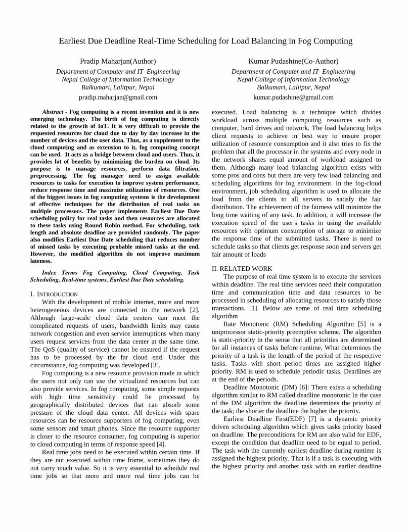
Earliest Due Deadline Real-Time Scheduling for Load Balancing in Fog Computing
Pradip Maharjan(Author) Kumar Pudashine(Co-Author)
Department of Computer and IT Engineering Department of Computer and IT Engineering
Nepal College of Information Technology Nepal College of Information Technology
Balkumari, Lalitpur, Nepal Balkumari, Lalitpur, Nepal
[email protected] [email protected]
Abstract - Fog computing is a recent invention and it is new
emerging technology. The birth of fog computing is directly
related to the growth of IoT. It is very difficult to provide the
requested resources for cloud due to day by day increase in the
number of devices and the user data. Thus, as a supplement to the
cloud computing and as extension to it, fog computing concept
can be used. It acts as a bridge between cloud and users. Thus, it
provides lot of benefits by minimizing the burden on cloud. Its
purpose is to manage resources, perform data filtration,
preprocessing. The fog manager need to assign available
resources to tasks for execution to improve system performance,
reduce response time and maximize utilization of resources. One
of the biggest issues in fog computing systems is the development
of effective techniques for the distribution of real tasks on
multiple processors. The paper implements Earliest Due Date
scheduling policy for real tasks and then resources are allocated
to these tasks using Round Robin method. For scheduling, task
length and absolute deadline are provided randomly. The paper
also modifies Earliest Due Date scheduling that reduces number
of missed tasks by executing probable missed tasks at the end.
However, the modified algorithm do not improve maximum
lateness.
Index Terms Fog Computing, Cloud Computing, Task
Scheduling, Real-time systems, Earliest Due Date scheduling.
I. INTRODUCTION
With the development of mobile internet, more and more
heterogeneous devices are connected to the network [2].
Although large-scale cloud data centers can meet the
complicated requests of users, bandwidth limits may cause
network congestion and even service interruptions when many
users request services from the data center at the same time.
The QoS (quality of service) cannot be ensured if the request
has to be processed by the far cloud end. Under this
circumstance, fog computing was developed [3].
Fog computing is a new resource provision mode in which
the users not only can use the virtualized resources but can
also provide services. In fog computing, some simple requests
with high time sensitivity could be processed by
geographically distributed devices that can absorb some
pressure of the cloud data center. All devices with spare
resources can be resource supporters of fog computing, even
some sensors and smart phones. Since the resource supporter
is closer to the resource consumer, fog computing is superior
to cloud computing in terms of response speed [4].
Real time jobs need to be executed within certain time. If
they are not executed within time frame, sometimes they do
not carry much value. So it is very essential to schedule real
time jobs so that more and more real time jobs can be
executed. Load balancing is a technique which divides
workload across multiple computing resources such as
computer, hard drives and network. The load balancing helps
client requests to achieve in best way to ensure proper
utilization of resource consumption and it also tries to fix the
problem that all the processor in the systems and every node in
the network shares equal amount of workload assigned to
them. Although many load balancing algorithm exists with
some pros and cons but there are very few load balancing and
scheduling algorithms for fog environment. In the fog-cloud
environment, job scheduling algorithm is used to allocate the
load from the clients to all servers to satisfy the fair
distribution. The achievement of the fairness will minimize the
long time waiting of any task. In addition, it will increase the
execution speed of the user's tasks in using the available
resources with optimum consumption of storage to minimize
the response time of the submitted tasks. There is need to
schedule tasks so that clients get response soon and servers get
fair amount of loads
II. RELATED WORK
The purpose of real time system is to execute the services
within deadline. The real time services need their computation
time and communication time and data resources to be
processed in scheduling of allocating resources to satisfy those
transactions. [1]. Below are some of real time scheduling
algorithm
Rate Monotonic (RM) Scheduling Algorithm [5] is a
uniprocessor static-priority preemptive scheme. The algorithm
is static-priority in the sense that all priorities are determined
for all instances of tasks before runtime. What determines the
priority of a task is the length of the period of the respective
tasks. Tasks with short period times are assigned higher
priority. RM is used to schedule periodic tasks. Deadlines are
at the end of the periods.
Deadline Monotonic (DM) [6]: There exists a scheduling
algorithm similar to RM called deadline monotonic In the case
of the DM algorithm the deadline determines the priority of
the task; the shorter the deadline the higher the priority.
Earliest Deadline First(EDF) [7] is a dynamic priority
driven scheduling algorithm which gives tasks priority based
on deadline. The preconditions for RM are also valid for EDF,
except the condition that deadline need to be equal to period.
The task with the currently earliest deadline during runtime is
assigned the highest priority. That is if a task is executing with
the highest priority and another task with an earlier deadline
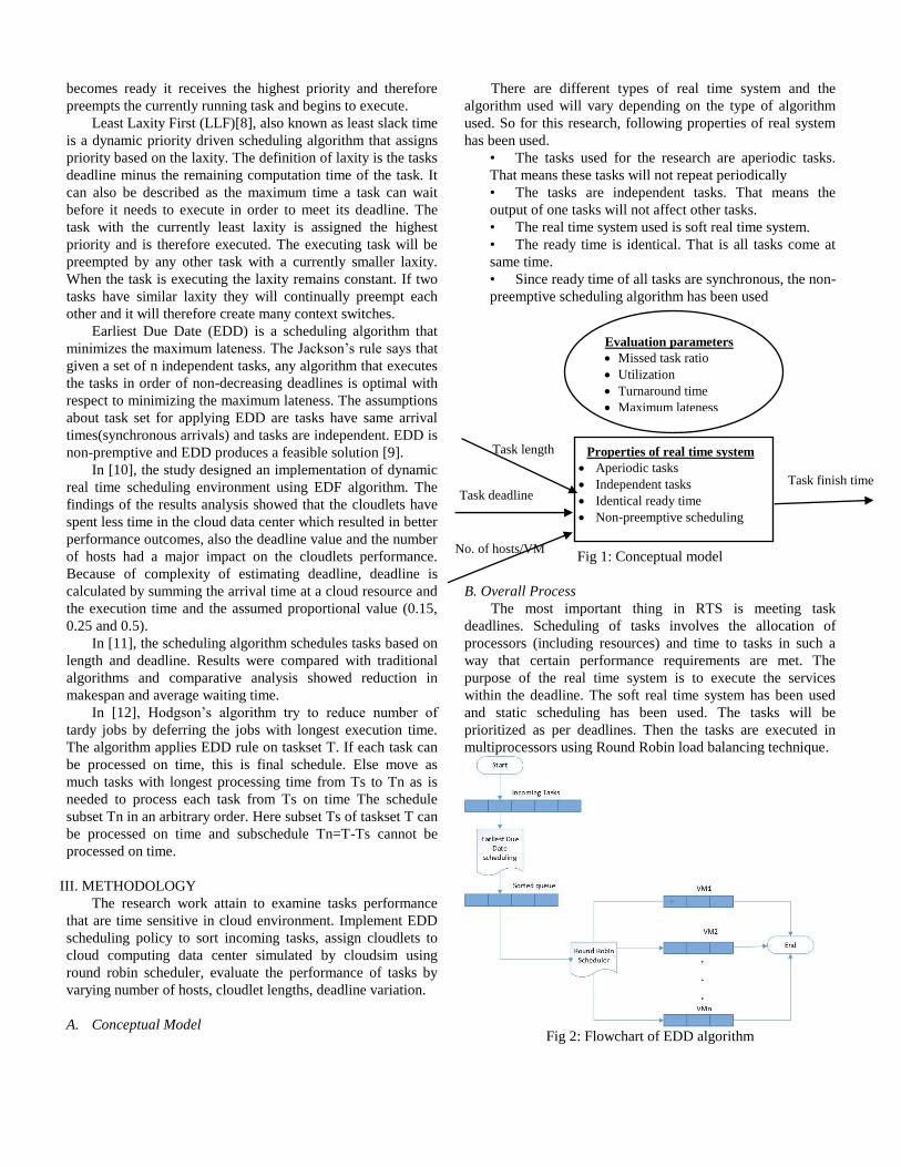
becomes ready it receives the highest priority and therefore
preempts the currently running task and begins to execute.
Least Laxity First (LLF)[8], also known as least slack time
is a dynamic priority driven scheduling algorithm that assigns
priority based on the laxity. The definition of laxity is the tasks
deadline minus the remaining computation time of the task. It
can also be described as the maximum time a task can wait
before it needs to execute in order to meet its deadline. The
task with the currently least laxity is assigned the highest
priority and is therefore executed. The executing task will be
preempted by any other task with a currently smaller laxity.
When the task is executing the laxity remains constant. If two
tasks have similar laxity they will continually preempt each
other and it will therefore create many context switches.
Earliest Due Date (EDD) is a scheduling algorithm that
minimizes the maximum lateness. The Jackson’s rule says that
given a set of n independent tasks, any algorithm that executes
the tasks in order of non-decreasing deadlines is optimal with
respect to minimizing the maximum lateness. The assumptions
about task set for applying EDD are tasks have same arrival
times(synchronous arrivals) and tasks are independent. EDD is
non-premptive and EDD produces a feasible solution [9].
In [10], the study designed an implementation of dynamic
real time scheduling environment using EDF algorithm. The
findings of the results analysis showed that the cloudlets have
spent less time in the cloud data center which resulted in better
performance outcomes, also the deadline value and the number
of hosts had a major impact on the cloudlets performance.
Because of complexity of estimating deadline, deadline is
calculated by summing the arrival time at a cloud resource and
the execution time and the assumed proportional value (0.15,
0.25 and 0.5).
In [11], the scheduling algorithm schedules tasks based on
length and deadline. Results were compared with traditional
algorithms and comparative analysis showed reduction in
makespan and average waiting time.
In [12], Hodgson’s algorithm try to reduce number of
tardy jobs by deferring the jobs with longest execution time.
The algorithm applies EDD rule on taskset T. If each task can
be processed on time, this is final schedule. Else move as
much tasks with longest processing time from Ts to Tn as is
needed to process each task from Ts on time The schedule
subset Tn in an arbitrary order. Here subset Ts of taskset T can
be processed on time and subschedule Tn=T-Ts cannot be
processed on time.
III. METHODOLOGY
The research work attain to examine tasks performance
that are time sensitive in cloud environment. Implement EDD
scheduling policy to sort incoming tasks, assign cloudlets to
cloud computing data center simulated by cloudsim using
round robin scheduler, evaluate the performance of tasks by
varying number of hosts, cloudlet lengths, deadline variation.
A. Conceptual Model
There are different types of real time system and the
algorithm used will vary depending on the type of algorithm
used. So for this research, following properties of real system
has been used.
• The tasks used for the research are aperiodic tasks.
That means these tasks will not repeat periodically
• The tasks are independent tasks. That means the
output of one tasks will not affect other tasks.
• The real time system used is soft real time system.
• The ready time is identical. That is all tasks come at
same time.
• Since ready time of all tasks are synchronous, the non-
preemptive scheduling algorithm has been used
Fig 1: Conceptual model
B. Overall Process
The most important thing in RTS is meeting task
deadlines. Scheduling of tasks involves the allocation of
processors (including resources) and time to tasks in such a
way that certain performance requirements are met. The
purpose of the real time system is to execute the services
within the deadline. The soft real time system has been used
and static scheduling has been used. The tasks will be
prioritized as per deadlines. Then the tasks are executed in
multiprocessors using Round Robin load balancing technique.
Fig 2: Flowchart of EDD algorithm
Task length
No. of hosts/VM
Task finish time Task deadline
Properties of real time system
Aperiodic tasks
Independent tasks
Identical ready time
Non-preemptive scheduling
Evaluation parameters
Missed task ratio
Utilization
Turnaround time
Maximum lateness
Guarantee ratio
Utilization
Turnaroud time
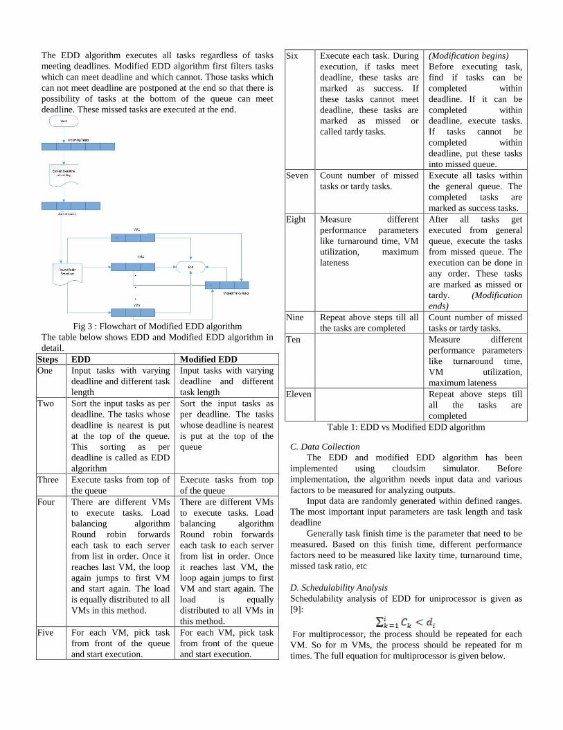
The EDD algorithm executes all tasks regardless of tasks
meeting deadlines. Modified EDD algorithm first filters tasks
which can meet deadline and which cannot. Those tasks which
can not meet deadline are postponed at the end so that there is
possibility of tasks at the bottom of the queue can meet
deadline. These missed tasks are executed at the end.
Fig 3 : Flowchart of Modified EDD algorithm
The table below shows EDD and Modified EDD algorithm in
detail.
Steps EDD Modified EDD
One Input tasks with varying
deadline and different task
length
Input tasks with varying
deadline and different
task length
Two Sort the input tasks as per
deadline. The tasks whose
deadline is nearest is put
at the top of the queue.
This sorting as per
deadline is called as EDD
algorithm
Sort the input tasks as
per deadline. The tasks
whose deadline is nearest
is put at the top of the
queue
Three Execute tasks from top of
the queue
Execute tasks from top
of the queue
Four There are different VMs
to execute tasks. Load
balancing algorithm
Round robin forwards
each task to each server
from list in order. Once it
reaches last VM, the loop
again jumps to first VM
and start again. The load
is equally distributed to all
VMs in this method.
There are different VMs
to execute tasks. Load
balancing algorithm
Round robin forwards
each task to each server
from list in order. Once
it reaches last VM, the
loop again jumps to first
VM and start again. The
load is equally
distributed to all VMs in
this method.
Five For each VM, pick task
from front of the queue
and start execution.
For each VM, pick task
from front of the queue
and start execution.
Six Execute each task. During
execution, if tasks meet
deadline, these tasks are
marked as success. If
these tasks cannot meet
deadline, these tasks are
marked as missed or
called tardy tasks.
(Modification begins)
Before executing task,
find if tasks can be
completed within
deadline. If it can be
completed within
deadline, execute tasks.
If tasks cannot be
completed within
deadline, put these tasks
into missed queue.
Seven Count number of missed
tasks or tardy tasks.
Execute all tasks within
the general queue. The
completed tasks are
marked as success tasks.
Eight Measure different
performance parameters
like turnaround time, VM
utilization, maximum
lateness
After all tasks get
executed from general
queue, execute the tasks
from missed queue. The
execution can be done in
any order. These tasks
are marked as missed or
tardy. (Modification
ends)
Nine Repeat above steps till all
the tasks are completed
Count number of missed
tasks or tardy tasks.
Ten Measure different
performance parameters
like turnaround time,
VM utilization,
maximum lateness
Eleven Repeat above steps till
all the tasks are
completed
Table 1: EDD vs Modified EDD algorithm
C. Data Collection
The EDD and modified EDD algorithm has been
implemented using cloudsim simulator. Before
implementation, the algorithm needs input data and various
factors to be measured for analyzing outputs.
Input data are randomly generated within defined ranges.
The most important input parameters are task length and task
deadline
Generally task finish time is the parameter that need to be
measured. Based on this finish time, different performance
factors need to be measured like laxity time, turnaround time,
missed task ratio, etc
D. Schedulability Analysis
Schedulability analysis of EDD for uniprocessor is given as
[9]:
For multiprocessor, the process should be repeated for each
VM. So for m VMs, the process should be repeated for m
times. The full equation for multiprocessor is given below.
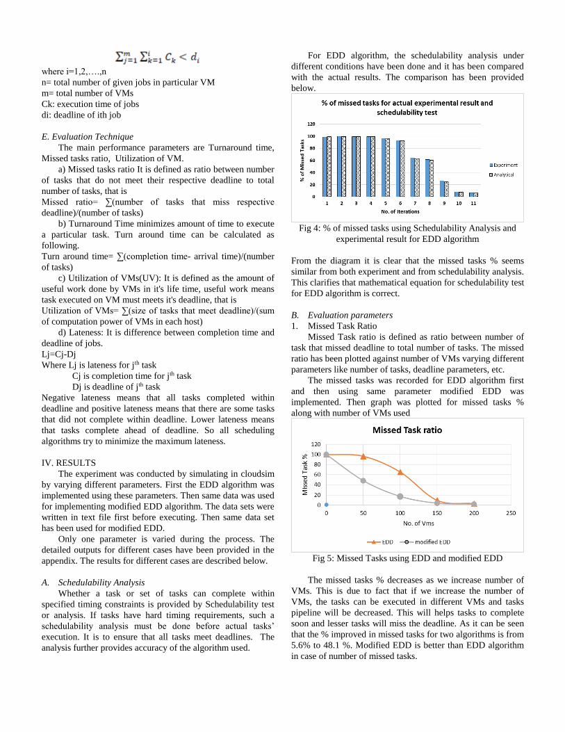
where i=1,2,….,n
n= total number of given jobs in particular VM
m= total number of VMs
Ck: execution time of jobs
di: deadline of ith job
E. Evaluation Technique
The main performance parameters are Turnaround time,
Missed tasks ratio, Utilization of VM.
a) Missed tasks ratio It is defined as ratio between number
of tasks that do not meet their respective deadline to total
number of tasks, that is
Missed ratio= ∑(number of tasks that miss respective
deadline)/(number of tasks)
b) Turnaround Time minimizes amount of time to execute
a particular task. Turn around time can be calculated as
following.
Turn around time= ∑(completion time- arrival time)/(number
of tasks)
c) Utilization of VMs(UV): It is defined as the amount of
useful work done by VMs in it's life time, useful work means
task executed on VM must meets it's deadline, that is
Utilization of VMs= ∑(size of tasks that meet deadline)/(sum
of computation power of VMs in each host)
d) Lateness: It is difference between completion time and
deadline of jobs.
Lj=Cj-Dj
Where Lj is lateness for jth task
Cj is completion time for jth task
Dj is deadline of jth task
Negative lateness means that all tasks completed within
deadline and positive lateness means that there are some tasks
that did not complete within deadline. Lower lateness means
that tasks complete ahead of deadline. So all scheduling
algorithms try to minimize the maximum lateness.
IV. RESULTS
The experiment was conducted by simulating in cloudsim
by varying different parameters. First the EDD algorithm was
implemented using these parameters. Then same data was used
for implementing modified EDD algorithm. The data sets were
written in text file first before executing. Then same data set
has been used for modified EDD.
Only one parameter is varied during the process. The
detailed outputs for different cases have been provided in the
appendix. The results for different cases are described below.
A. Schedulability Analysis
Whether a task or set of tasks can complete within
specified timing constraints is provided by Schedulability test
or analysis. If tasks have hard timing requirements, such a
schedulability analysis must be done before actual tasks’
execution. It is to ensure that all tasks meet deadlines. The
analysis further provides accuracy of the algorithm used.
For EDD algorithm, the schedulability analysis under
different conditions have been done and it has been compared
with the actual results. The comparison has been provided
below.
Fig 4: % of missed tasks using Schedulability Analysis and
experimental result for EDD algorithm
From the diagram it is clear that the missed tasks % seems
similar from both experiment and from schedulability analysis.
This clarifies that mathematical equation for schedulability test
for EDD algorithm is correct.
B. Evaluation parameters
1. Missed Task Ratio
Missed Task ratio is defined as ratio between number of
task that missed deadline to total number of tasks. The missed
ratio has been plotted against number of VMs varying different
parameters like number of tasks, deadline parameters, etc.
The missed tasks was recorded for EDD algorithm first
and then using same parameter modified EDD was
implemented. Then graph was plotted for missed tasks %
along with number of VMs used
Fig 5: Missed Tasks using EDD and modified EDD
The missed tasks % decreases as we increase number of
VMs. This is due to fact that if we increase the number of
VMs, the tasks can be executed in different VMs and tasks
pipeline will be decreased. This will helps tasks to complete
soon and lesser tasks will miss the deadline. As it can be seen
that the % improved in missed tasks for two algorithms is from
5.6% to 48.1 %. Modified EDD is better than EDD algorithm
in case of number of missed tasks.
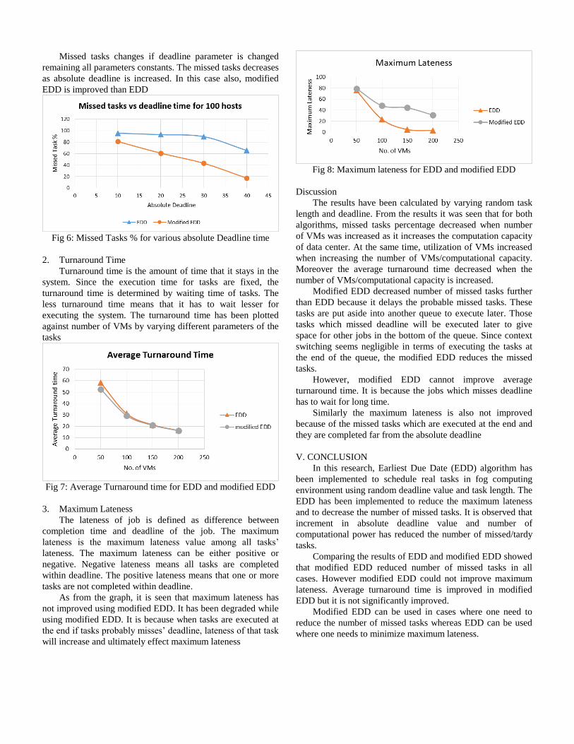
Missed tasks changes if deadline parameter is changed
remaining all parameters constants. The missed tasks decreases
as absolute deadline is increased. In this case also, modified
EDD is improved than EDD
Fig 6: Missed Tasks % for various absolute Deadline time
2. Turnaround Time
Turnaround time is the amount of time that it stays in the
system. Since the execution time for tasks are fixed, the
turnaround time is determined by waiting time of tasks. The
less turnaround time means that it has to wait lesser for
executing the system. The turnaround time has been plotted
against number of VMs by varying different parameters of the
tasks
Fig 7: Average Turnaround time for EDD and modified EDD
3. Maximum Lateness
The lateness of job is defined as difference between
completion time and deadline of the job. The maximum
lateness is the maximum lateness value among all tasks’
lateness. The maximum lateness can be either positive or
negative. Negative lateness means all tasks are completed
within deadline. The positive lateness means that one or more
tasks are not completed within deadline.
As from the graph, it is seen that maximum lateness has
not improved using modified EDD. It has been degraded while
using modified EDD. It is because when tasks are executed at
the end if tasks probably misses’ deadline, lateness of that task
will increase and ultimately effect maximum lateness
Fig 8: Maximum lateness for EDD and modified EDD
Discussion
The results have been calculated by varying random task
length and deadline. From the results it was seen that for both
algorithms, missed tasks percentage decreased when number
of VMs was increased as it increases the computation capacity
of data center. At the same time, utilization of VMs increased
when increasing the number of VMs/computational capacity.
Moreover the average turnaround time decreased when the
number of VMs/computational capacity is increased.
Modified EDD decreased number of missed tasks further
than EDD because it delays the probable missed tasks. These
tasks are put aside into another queue to execute later. Those
tasks which missed deadline will be executed later to give
space for other jobs in the bottom of the queue. Since context
switching seems negligible in terms of executing the tasks at
the end of the queue, the modified EDD reduces the missed
tasks.
However, modified EDD cannot improve average
turnaround time. It is because the jobs which misses deadline
has to wait for long time.
Similarly the maximum lateness is also not improved
because of the missed tasks which are executed at the end and
they are completed far from the absolute deadline
V. CONCLUSION
In this research, Earliest Due Date (EDD) algorithm has
been implemented to schedule real tasks in fog computing
environment using random deadline value and task length. The
EDD has been implemented to reduce the maximum lateness
and to decrease the number of missed tasks. It is observed that
increment in absolute deadline value and number of
computational power has reduced the number of missed/tardy
tasks.
Comparing the results of EDD and modified EDD showed
that modified EDD reduced number of missed tasks in all
cases. However modified EDD could not improve maximum
lateness. Average turnaround time is improved in modified
EDD but it is not significantly improved.
Modified EDD can be used in cases where one need to
reduce the number of missed tasks whereas EDD can be used
where one needs to minimize maximum lateness.

REFERENCES [1] Verma M., Bhardwaj N., Yadav A. K.,"Real Time Efficient
Scheduling Algorithm for Load Balancing in Fog Computing
Environment", International Journal of Information Technology and
Computer Science(IJITCS), Vol.8, No.4, pp.1-10, 2016. DOI:
10.5815/ijitcs.
[2] Zhang, J., Simplot-Ryl, D., Bisdikian, C., Mouftah, H.T., 2011.
The internet of things. IEEE Commun. Mag. 49 (11), 30–31.
[3] Bonomi, F., Milito, R., Zhu, J., Addepalli, S., 2012. “Fog
computing and its role in the internet of things”. In: Proceedings of
the first edition of the MCC workshop on Mobile cloud computing,
ACM, pp. 13–16
[4] Sun Y., Zhang N. "A resource-sharing model based on a repeated
game in fog computing" Saudi Journal of Biological Sciences (2017)
24, 687–694
[5] Liu C.L. and Layland J.W., "Scheduling Algorithms for
Multiprogramming in a Hard-Real-Time Environment" Journal of the
Association for Computing Machinery, vol. 20, no. 1, pp. 46-61.,
year 1973
[6] Leung J. Y.-T., Whitehead J., "On the complexity of fixed priority
scheduling of periodic, real-time tasks", Performance Evaluation, vol.
2, issue 4, pages 237-250, December 1982.
[7] Burns A. and Audsley N., "REAL-TIME SYSTEM
SCHEDULING" Predicatably Dependable Computer Systems,
Volume 2, Chapter 2, Part II. or Department of Computer Science,
University of York, UK
[8] Dertouzos M.L. and Mok A.K.L., "Multiprocessor On-Line
Scheduling of Hard Real-Time Tasks" IEEE Transactions on
Software Engineering, vol. 15, no. 12, December 1989
[9] Buttazzo G.C., “Hard Real-Time Computing Systems Predictable
Scheduling Algorithms and Applications” Third Edition, Springer,
2011
[10] Ali S. K. F., Hamad M. B., “Implementation of an EDF
Algorithm in a Cloud Computing Environment using the CloudSim
Tool” International Conference on Computing, Control, Networking,
Electronics and Embedded Systems Engineering, 2015
[11] Wadhnokar A., Theng D., “ A Task Scheduling Algorithm
Based on Task Length and Deadline in Cloud Computing”,
International Journal of Scientific & Engineering Research, Volume
7, Issue 4, April-2016
[12] J. Błażewicz, K. H. Ecker, E. Pesch, G. Schmidt, and J.
Węglarz. Scheduling Computer and Manufacturing Process.
Springer. 2nd printing. 2001. 3-540-41931-4

Systematic Management of SIM Cards
Sujana Shakya
Nepal College of Information Technology
Balkumari, Lalitpur
Niki Maharjan
Nepal College of Information Technology
Balkumari, Lalitpur
Abstract
This is the research paper based on systematic
management of sim cards. Generally, it can also be
termed as the inventory management of sim cards. This
system normally keeps the record of the sales, purchase
or the sim cards for the particular interval of time.as of
this system is designed for the retailers who are
assigned by the telecommunication company for selling
sim cards. Here, in this study, systematic management
of sim card is for keeping the records of sim cards with
its serial number, phone number, pin number, PUK code
and all related codes. The main objective of this study is
to terminate the traditional entry of the sim cards which
was initially written in a form by hands and are stored
in piles of file and systematically enter the details of the
sim card. The details of the sim card along with the
details of buyer is stored in the database systematically
so that it can be used for future purpose as well.
Acquiring systematic entry of sim card details is highly
recommended by this system so that the data would not
get lost.
Keywords: traditional, SIM cards, purchase, inventory,
sales, customers, management.
I. INTRODUCTION
Inventory management system refer to the management
of the physical resource which is hold by the business
with some specific objective for balancing the need of
availability of the products. It is used for automating the
sales in order to fulfill the process. Generally inventory
management is for keeping the track of the resources
through unique codes such as barcodes, serial number
which is provided by the operator themselves. It is an
approach to take supply chain as a whole rather than
taking it separately for some specific purpose.[1]
Inventory management system is for maintaining the
stocks that are kept in the ware house. The tracking and
monitoring the use of the stocks helps in making the
reports of the inventory status.[7] The cost can also be
minimized with such kind of system. The inventory
management system (IMS) helps any kind of business
to analyze their processes related to sales and purchase
of the products to make effective decision about
inventory.[8]
In this study we are researching about the inventory
management of the sim cards in the context of Nepal. In
Nepal there are only three vendors via Nepal Telecom,
Ncell and Smart Cell. In this system the details of sim
cards will be entered in bulk. The sim cards will be
provided by the telecommunication company to the
retailers. The retailers get the physical sim cards along
with the excel sheet of the sim card numbers in bulk
amount from the respective telecommunication
company and sell them either to the individuals or to
other resellers. Here, we mainly focus on purchase, sell
and inventory management of the SIM cards that are
hold by the retailer company. In this system, we entry
the customer details and the SIM card number of the
SIM they have bought for registration. With this project,
it will be easier for the retailer company to keep histories
of the SIM card they have sold and they have given for
sale. The archive of customer details along with their
respective SIM card number is kept in the database of
Retailer Company and for the official registration of
SIM card they send a file to the telecommunication
company themselves. The main objective of this project
is to minimize manual process of purchasing SIM card
and to manage the purchased SIM from Telecom
Company and the SIM cards that have been sold to the
customers.

Inventory management can be applied for the
calculation of the quantities as well as managing the
physical resource and its monetary value. [6]
II. PROBLEM STATEMENT
In the context of Nepal there are only three
Telecommunication Company and the people from all
over the country are dependent upon the sim cards from
those three companies only. People mostly buy the sim
cards from the retailers rather than buying the sim card
directly from the telecommunication company. When
the customer buys the sim card from the retailer they are
supposed to fill up the form with their personal details
manually, then it is stored by the retailer and handover
the physical sim card to the buyer. The problem that
occurs here is that the seller will have to write each and
every detail of the customer as well as the sim card they
hold and the chances that the paper may get lost,
destroy, damage due to which when that paper is needed
it cannot be made available. The retailer company will
not have the exact details of how much sim cards have
been sold and the quantity remained in the stock so as
how much they have earned selling sim cards coming
from each vendor.
III. OBJECTIVES
Every research is conducted with certain objectives. The
main objectives of this research are as follows:
• To provide automated system to the retailers for
keeping proper record of simcards coming from
different vendors.
• To store the information of the customer in the
database for future use.
• To keep the systematic record of the sim cards
corresponding to its serial number received by
reseller in bulk amount by the company.
• To prevent the data from getting lost and
misplaced as the data will be stored in the
database with proper backup.
IV. Literature Review
Review
Sim cards are mandatory if you have a cellphone and
you want communication medium. Every cellphone
holder needs a sim card. People buys the SIM card of
any telecommunication company they want. The
telecom company doesn’t sell the SIM cards on their
own, so they assign various retailers to sell their SIM
card. To manage all the SIM cards provided by the
telecom company, this kind of system is a must to keep
systematic records of the SIM cards that have been sold
by the retailers.
Inventory Management and its benefits
Inventory management is a requirement of every
businesses. It is for keeping the systematic records of all
the stocks that the businesses hold. There are several
benefits of inventory management such as it helps to
take smart business decisions going through all the
obstacles and challenges, it will report about all the
products related with its sales and the businesses can
also know about the expenditures they have made on the
product. [9]
Related Study
Bession Low-Code Telecom Solutions
Bession Inventory Management system tracks plastic
cards for all SIM card sizes (standard, micro, Nano,
eSim) and it securely stores and manages all SIM card
information, including the ICCID, PIN/PUK codes. It
also manages all available phone numbers. This system
manages thousands of users. [12]
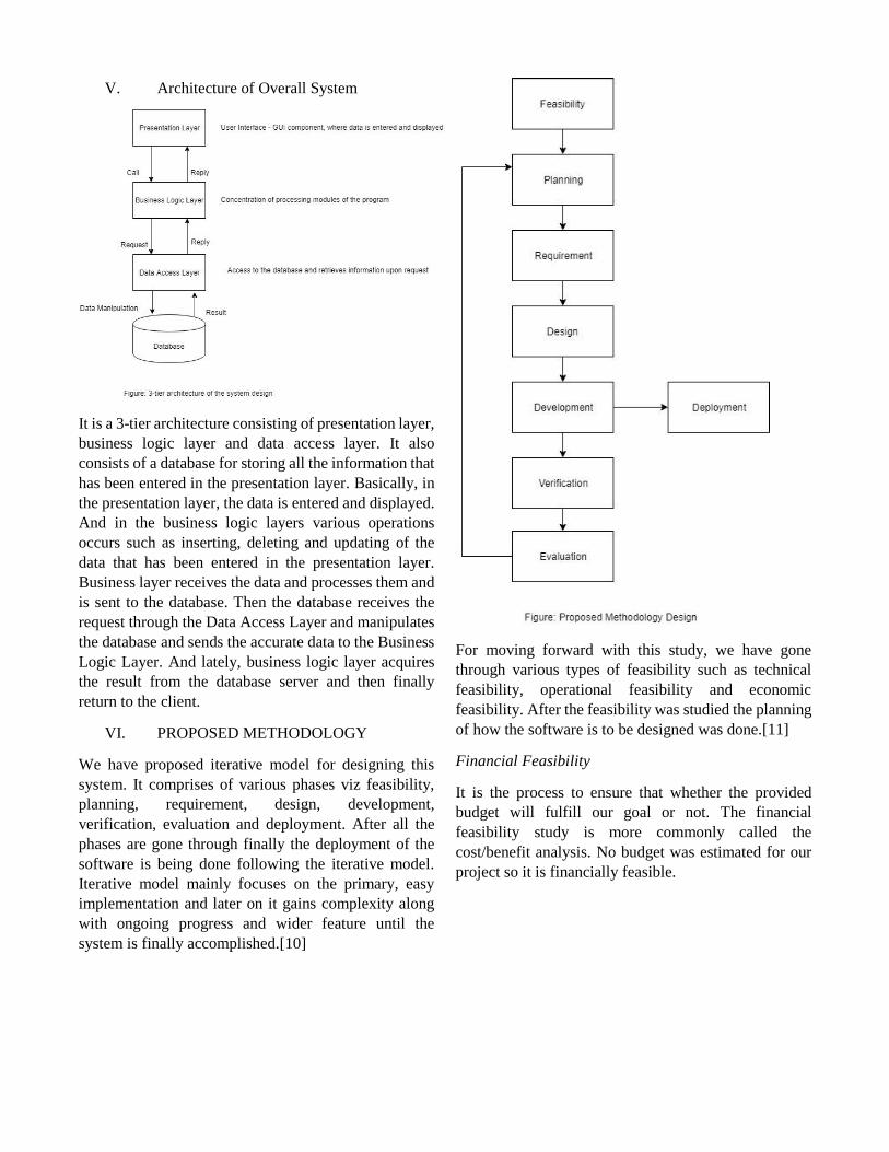
V. Architecture of Overall System
It is a 3-tier architecture consisting of presentation layer,
business logic layer and data access layer. It also
consists of a database for storing all the information that
has been entered in the presentation layer. Basically, in
the presentation layer, the data is entered and displayed.
And in the business logic layers various operations
occurs such as inserting, deleting and updating of the
data that has been entered in the presentation layer.
Business layer receives the data and processes them and
is sent to the database. Then the database receives the
request through the Data Access Layer and manipulates
the database and sends the accurate data to the Business
Logic Layer. And lately, business logic layer acquires
the result from the database server and then finally
return to the client.
VI. PROPOSED METHODOLOGY
We have proposed iterative model for designing this
system. It comprises of various phases viz feasibility,
planning, requirement, design, development,
verification, evaluation and deployment. After all the
phases are gone through finally the deployment of the
software is being done following the iterative model.
Iterative model mainly focuses on the primary, easy
implementation and later on it gains complexity along
with ongoing progress and wider feature until the
system is finally accomplished.[10]
For moving forward with this study, we have gone
through various types of feasibility such as technical
feasibility, operational feasibility and economic
feasibility. After the feasibility was studied the planning
of how the software is to be designed was done.[11]
Financial Feasibility
It is the process to ensure that whether the provided
budget will fulfill our goal or not. The financial
feasibility study is more commonly called the
cost/benefit analysis. No budget was estimated for our
project so it is financially feasible.

Technical Feasibility
It is the process to ensure that whether the given
technology can support requirements
or that a goal is technically possible.
In context to our system we already had a necessary
technical equipment’s and thereby the codes were all
written by our self so our system is technically feasible.
Operational Feasibility
It is the process of deploying and operating a project.
since the system is not publicly established yet but in
context to the current telecommunication company
situation all the requirements have be fulfilled so it is
operationally feasible.
The requirements was then collected and the software
was designed and developed and the verification and
evaluation of the software was carried out and finally
after finishing all these processes the deployment of the
software was finished.
VI. CONCLUSION
Thus, using proposed research methodology and various
theories related to inventory management this system
will be built for the ease of both the customer and the
retailer. There will be proper detail of the customer who
bought the sim card with which it will also be easier to
track the person in case of corruption by that person
related to thefts or criminal activities. The systematic
management will also prevent data from getting lost and
misuse.
ACKNOWLEDGEMENT
This systematic management of SIM card would not
have been possible without the support of Mr. Madan
Kadariya, IT Department, NCIT College. I express my
gratitude to Mr. Rabi Shakya for his immense support
and guidance for drafting this paper.
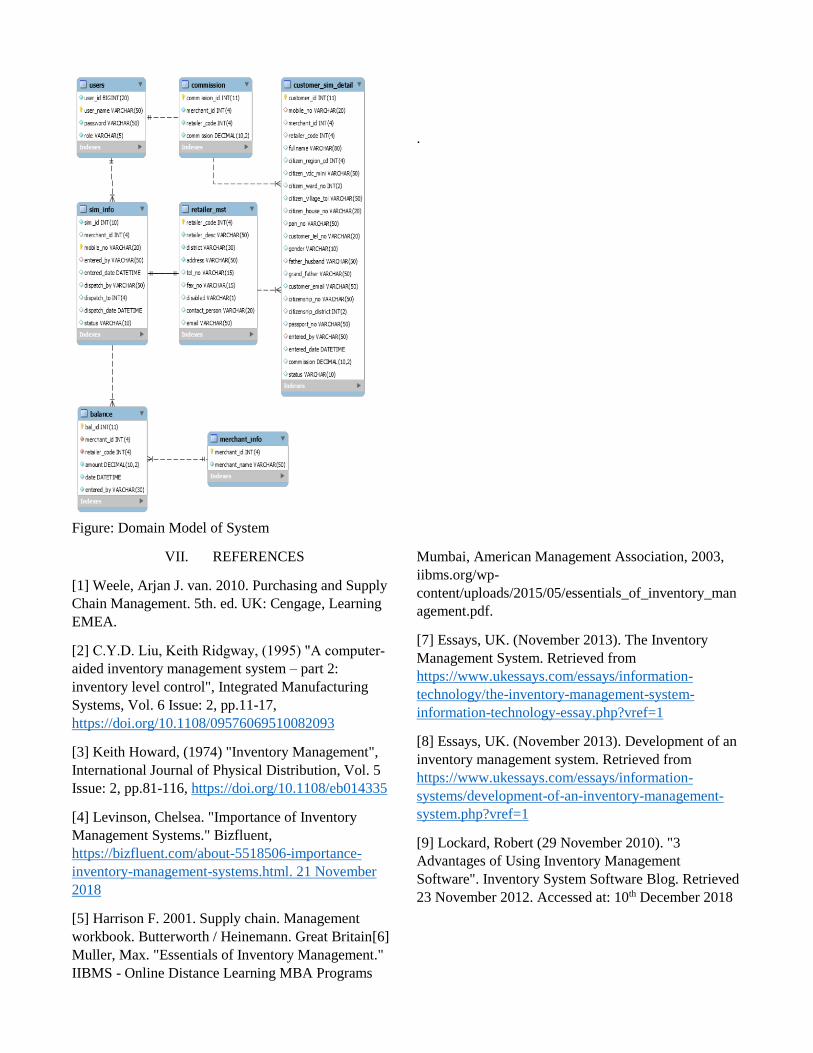
Figure: Domain Model of System
.
VII. REFERENCES
[1] Weele, Arjan J. van. 2010. Purchasing and Supply
Chain Management. 5th. ed. UK: Cengage, Learning
EMEA.
[2] C.Y.D. Liu, Keith Ridgway, (1995) "A computer‐
aided inventory management system – part 2:
inventory level control", Integrated Manufacturing
Systems, Vol. 6 Issue: 2, pp.11-17,
https://doi.org/10.1108/09576069510082093
[3] Keith Howard, (1974) "Inventory Management",
International Journal of Physical Distribution, Vol. 5
Issue: 2, pp.81-116, https://doi.org/10.1108/eb014335
[4] Levinson, Chelsea. "Importance of Inventory
Management Systems." Bizfluent,
https://bizfluent.com/about-5518506-importance-
inventory-management-systems.html. 21 November
2018
[5] Harrison F. 2001. Supply chain. Management
workbook. Butterworth / Heinemann. Great Britain[6]
Muller, Max. "Essentials of Inventory Management."
IIBMS - Online Distance Learning MBA Programs
Mumbai, American Management Association, 2003,
iibms.org/wp-
content/uploads/2015/05/essentials_of_inventory_man
agement.pdf.
[7] Essays, UK. (November 2013). The Inventory
Management System. Retrieved from
https://www.ukessays.com/essays/information-
technology/the-inventory-management-system-
information-technology-essay.php?vref=1
[8] Essays, UK. (November 2013). Development of an
inventory management system. Retrieved from
https://www.ukessays.com/essays/information-
systems/development-of-an-inventory-management-
system.php?vref=1
[9] Lockard, Robert (29 November 2010). "3
Advantages of Using Inventory Management
Software". Inventory System Software Blog. Retrieved
23 November 2012. Accessed at: 10th December 2018

[10] Powell-Morse, Andrew. "Iterative Model: What Is
It And When Should You Use It?" Airbrake Blog, 2
Nov. 2017, airbrake.io/blog/sdlc/iterative-
model?fbclid=IwAR3UD5TPzMoVYhOTjIfx7ZTjT0l
e_mlmDbDgNgWR5OKTyLYMxIMLb7Hw6M8.
Accessed 8 Dec. 2018.
[11] Spacey, John. "7 Types of Feasibility Analysis."
Simplicable, 24 Nov. 2017,
simplicable.com/new/feasibility-analysis. Accessed 5
Dec. 2018.
[12] Staff, Beesion. "Telecom Inventory Management."
Beesion Technologies, 16 Oct. 2018,
beesion.com/inventory-
management/?fbclid=IwAR1oUTYdqJqs87ev3I_DK0
mPi6fyGprSZyzpbLq-E3i0Ub2g705w0wt9YVM.
Accessed 11 Dec. 2018.
1
Weather Research and Forecasting Application Performance
Benchmark using MPICH and OpenMPI
Raksha Roy1, Sanjeeb Prasad Pandey2 Nepal College of Information Technology
ABSTRACT Last few decades have experienced an unprecedented use of multi-core and
multiprocessor architectures for building systems with high computational power. A large
number of Message Passing Interface (MPI) implementations are currently available,
each of which emphasize different aspects of high-performance computing and are
intended to solve specific research problem. Weather Research and Forecast (WRF)
model’s performance is crucial for saving computing time. This is important because
computing time in general is resource intensive and hence highly expensive. This research
implements MPICH and OPENMPI as MPI’s API, for shared and distributed parallelism
using WRF Application. WRF build times were calculated with increasing number of
cores and WRF runs were carried out on number of processors ranging from 5 till 30 in
DMPar mode, and from 5 to 20 in SMPar mode. WRF run times showed significant
change in SMPar with linear curve while in DMPar mode, it showed a non-linear curve
with increase in number of processors both in MPICH and OPENMPI. The time taken to
run WRF using DMPar mode in MPICH is lesser than in OpenMPI. In SMPar mode,
WRF takes lesser time to run in OpenMPI than MPICH. The findings were such that
DMPar functions better, in terms of time taken to run WRF, in MPICH and SMPar
functions better in OpenMPI.
Keywords: Weather Research and Forecast, high performance computing, MPICH,
OPENMPI, DMPar, SMPar Distributed Memory, Shared Memory, Run Time
1. INTRODUCTION
The Weather Research and Forecasting
(WRF) Model is an atmospheric model
designed for both research and
numerical weather prediction (NWP).
WRF Model is a next-generation
mesoscale numerical weather prediction
system designed for both atmospheric
research and operational forecasting
applications. The model serves a wide
range of meteorological applications
across scales from tens of meters to
thousands of kilometers. One of the
major features of WRF model is its
software architecture which supports
parallel computation and system
extensibility.
OpenMPI is a particular Application
Programming Interface (API) of
Message Passing Interface (MPI)
whereas OpenMP is shared
memory standard available with
compiler. These APIs are basically
intended to parallel programming or
parallel computation using OpenMP or
MPICH for applications. MPIs are
available as API of in library form for C,
C++ and FORTRAN. There are
numerous MPI’s API available in the
market, such as, OpenMPI, MPICH, HP-
MPI, Intel MPI, etc. Among them,
OpenMPI and MPICH, which are chosen
for this research purpose are freely
available and does not require license.
These APIs can be used to parallelize
programs. MPI standards maintain that
all of these APIs provided by different
vendors or groups follow similar
standards, so all functions or subroutines
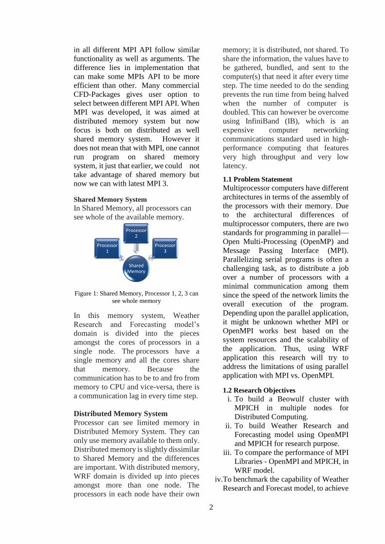
2
in all different MPI API follow similar
functionality as well as arguments. The
difference lies in implementation that
can make some MPIs API to be more
efficient than other. Many commercial
CFD-Packages gives user option to
select between different MPI API. When
MPI was developed, it was aimed at
distributed memory system but now
focus is both on distributed as well
shared memory system. However it
does not mean that with MPI, one cannot
run program on shared memory
system, it just that earlier, we could not
take advantage of shared memory but
now we can with latest MPI 3.
Shared Memory System
In Shared Memory, all processors can
see whole of the available memory.
Figure 1: Shared Memory, Processor 1, 2, 3 can
see whole memory
In this memory system, Weather
Research and Forecasting model’s
domain is divided into the pieces
amongst the cores of processors in a
single node. The processors have a
single memory and all the cores share
that memory. Because the
communication has to be to and fro from
memory to CPU and vice-versa, there is
a communication lag in every time step.
Distributed Memory System
Processor can see limited memory in
Distributed Memory System. They can
only use memory available to them only.
Distributed memory is slightly dissimilar
to Shared Memory and the differences
are important. With distributed memory,
WRF domain is divided up into pieces
amongst more than one node. The
processors in each node have their own
memory; it is distributed, not shared. To
share the information, the values have to
be gathered, bundled, and sent to the
computer(s) that need it after every time
step. The time needed to do the sending
prevents the run time from being halved
when the number of computer is
doubled. This can however be overcome
using InfiniBand (IB), which is an
expensive computer networking
communications standard used in high-
performance computing that features
very high throughput and very low
latency.
1.1 Problem Statement
Multiprocessor computers have different
architectures in terms of the assembly of
the processors with their memory. Due
to the architectural differences of
multiprocessor computers, there are two
standards for programming in parallel—
Open Multi-Processing (OpenMP) and
Message Passing Interface (MPI).
Parallelizing serial programs is often a
challenging task, as to distribute a job
over a number of processors with a
minimal communication among them
since the speed of the network limits the
overall execution of the program.
Depending upon the parallel application,
it might be unknown whether MPI or
OpenMPI works best based on the
system resources and the scalability of
the application. Thus, using WRF
application this research will try to
address the limitations of using parallel
application with MPI vs. OpenMPI.
1.2 Research Objectives
i. To build a Beowulf cluster with
MPICH in multiple nodes for
Distributed Computing.
ii. To build Weather Research and
Forecasting model using OpenMPI
and MPICH for research purpose.
iii. To compare the performance of MPI
Libraries - OpenMPI and MPICH, in
WRF model.
iv.To benchmark the capability of Weather
Research and Forecast model, to achieve
Shared Memory
Processor 1
Processor 2
Processor 3
3
scalable productivity at increasing core
counts.
1.3 Significance of the Study
The goal of the parallel programming is
to reduce the execution time, idle time
and communication time. Both the MPI
and OpenMPI standards have
similarities in various implementations
such as source code compatibility
(except parallel I/O) and support for
heterogeneous parallel architectures
such as clusters, grids, groups of
workstations, SMP computers and etc.
One of the major difference is the
programming approaches that undergo
SMPD and MPMD. This research
approach is anticipated to help
researchers, scientists, WRF users and
community to choose between the
distributed vs. shared algorithm based on
the CPU architectures, cores, scalability
of the application and other available
system resources.
2. METHODOLOGY The model for parallelism is related
relatively closely to the hardware the
model runs on. In installation of Weather
Research and Forecasting application,
Shared-memory Parallelism (SMPar) is
for multi-core/multi CPUs, and
Distributed-memory Parallelism
(DMPar) is for clusters. In practice what
happens is that OpenMP directives are
enabled and the resulting binary will
only run within a single shared-memory
system. This option is not highly tested,
however, and is usually not
recommended. The resulting binary will
run within and across multiple nodes of
a distributed-memory system (or
cluster). We can also configure for a
build that includes both SMPar and
DMPar. The resulting binary can be run
hybrid, meaning using OpenMP for
parallelism within nodes (total or partial)
and MPI across nodes. Getting a hybrid
build to have its OpenMP threads and
MPI tasks placed properly on the
processors can be difficult, though, and
this option is also not usually
recommended.
2.1 Cluster Configuration
In this research, focus is on OpenMP for
parallelism using the SMPar and DMPar
separately and then calculate the
performance of Weather Research and
Forecasting model on scalability.
Initially the system dependencies
including GNU C Compiler, v4.8.4 was
installed, and then the other prerequisites
for WRF application such as MPICH and
OpenMPI, NetCDF, HDF5, FLEX,
BISON and BYACC was installed. For
the research, Beowulf cluster was used.
One of the major requirements to create
a Beowulf cluster was to create a
password less SSH. Finally, Weather
Research and Forecasting model was
configured and built successfully .WRF
v3.8.1 model was run with grid
resolution of 5km X 5km for 12 hours
data set. The cluster is configured in
Dell™ PowerEdge™ M620 7-node
cluster with 2 X 10 core Intel (R)
Xeon(R) CPU E5-2660 v2 @ 2.20GHz.
The memory used in each node is 64 gb,
DDR3 1333 Mhz. Ubuntu 12.04 LTS is
the operating system used for the
research. The MPIs used are MPICH 3.2
and OpenMPI 2.0.2. The compiler
chosen was GNU Compiler 4.8.4 and a
miscellaneous package NetCDF 4.4.1.1.
The entire research is performed on a
parallel application- WRF (Weather
Research and Forecasting) v3.8.1. The
file system used is ext4.
2.2 Research Design
In a Distributed Memory, domain
contains patches in application, whereas
it contains tiles in shared memory.
Similarly, each system job runs in
processes in distributed memory
whereas it runs in threads in shared
memory. In distributed memory, the
hardware cluster is measured in nodes,
and in shared memory parallel it is
measured in processors.

4
Figure 2: Research Design in Distributed and
Shared Memory Parallel
WRF, WRF- Chem and WPS were
compiled using the tarballs. In first step
WRF was built from source, WRF-
Chem unzipped to WRF folder. The
second step included building WPS
from source.
3.3 Weather Research and Forecasting
Model build
The compilation was successful and the
following executables were created in
WRFV3/main:
1. ndown.exe
2. real.exe
3. tc.exe
4. wrf.exe
3.4 Weather Research and Forecasting
Preprocessor (WPS) Build
The compilation was successful and the
following executables were created in
WPS:
1. geogrid.exe
2. metgrid.exe
3. ungrib.exe
3.5 Weather Research and Forecasting
Compile using DMPAR – GFORTRAN
Weather Research and Forecasting
model was compiled in dmpar mode
using GFORTRAN compiler.
3.6 Data Collection Technique
The GRIB (GRIdded Binary or General
Regularly-distributed Information in
Binary form) data format sets taken for
the research is obtained from the
Computational and Information System
Laboratory at the National Center for
Atmospheric Research (NCAR) in
Boulder, Colorado.
For this research, 12 hours of data set of
January 15, 2016 was considered and the
area under consideration was for 5x5
km2.
4. RESULTS AND DISCUSSION
4.1 Weather Research and Forecasting
Application Build Time
The time taken by Weather Research and
Forecasting application was observed
against increasing numbers of cores. It
was observed that with increasing core
counts, the time taken to build WRF
decreased linearly. WRF Build Time
was recorded to be 12 minutes 59
seconds while WRF compiled using 1
socket and 6 core. Similarly, WRF Build
Time was recorded to be 13 minutes 46
seconds while WRF compiled in 1
socket and 5 core, 19 minutes 49 seconds
while WRF compiled with 1 socket and
2 core. WRF Build Time was recorded to
be 31 minutes 51 seconds while WRF
compiled using 1 socket and 1 core.
With increasing numbers of core, the
time taken for the Weather Research and
Forecasting model to build decreases
linearly. That is to say that WRF build
time depends on number of cores. This is
same in both the cases of DMPar and
SMPar mode. WRF run time depends on
mode that is being used to run the
application. But, unlike WRF run time,
WRF build time does not depend on
mode (DMPar mode or SMPar mode).
Distributed
Memory
Shared
Memory
Domain Patches Tiles
Job Processes Threads
Cluster Nodes Processors
APPLICATION
(WRF)
SYSTEM
(UNIX, MPI,
OpenMP)
HARDWARE
(Processors,
Memories,
Wires)

5
Figure 3: Weather Research and Forecasting
model build time (mins) using DMPar
WRF run time was measured across 5,
10,15,20,25 & 30 cores using DMPar
mode in MPICH and OpenMPI
respectively. While doing so, a non-
linear curve was obtained which showed
comparatively better performance of
DMPar mode in MPICH over OpenMPI.
Figure 4: Time (hrs) taken to run WRF using
DMPar in MPICH vs. OpenMPI
Similarly, WRF run time was measured
across 5, 10, 15 & 20 cores using SMPar
mode in MPICH and OpenMPI
respectively. While doing so, a non-
linear curve was obtained which showed
comparatively better performance of
SMPar in OpenMPI over MPICH.
Figure 5: Time (hrs) taken to run WRF using
SMPar in MPICH vs. OpenMPI
4.2 Efficiency Calculation of MPICH in
DMPar mode
Nos.
of
Cores
DMPar-
MPICH
DMPar-
OPENMPI Efficiency
Time
(hr) Time (hr)
(DMPar-MPICH
)
5 0.96 0.98 2.11
10 0.58 0.6 2.51
15 0.43 0.45 4.67
20 0.36 0.42 13.89(Peak
performance)
25 0.42 0.4 3.87
30 0.35 0.36 3.14
Table 1 : Efficiency calculation of MPICH in
DMPar mode
From table 1 above, in DMPar mode
using MPICH, it is seen that the peak
performance is obtained while using 20
cores. With the increase in the number of
cores, efficiency has gradually increased
up to 20 cores, thus generating a non-
linear graph. On 5 cores, DMPar mode is
seen 2.11% more efficient in MPICH
than in OPENMPI. Similarly on
10,15,20,15 and 30 cores, DMPAR is
2.51%, 4.67%, 13.89%, 3.87% and
3.14% efficient respectively. This
performance lag in DMPar mode is
basically observed due to
communication lag and network latency.
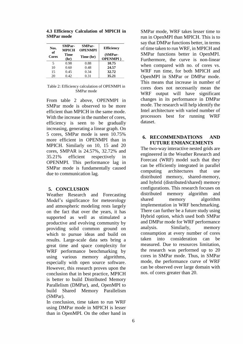
6
4.3 Efficiency Calculation of MPICH in
SMPar mode
Table 2: Efficiency calculation of OPENMPI in
SMPar mode
From table 2 above, OPENMPI in
SMPar mode is observed to be more
efficient than MPICH in the same mode.
With the increase in the number of cores,
efficiency is seen to be gradually
increasing, generating a linear graph. On
5 cores, SMPar mode is seen 10.75%
more efficient in OPENMPI than in
MPICH. Similarly on 10, 15 and 20
cores, SMPAR is 24.57%, 32.72% and
35.21% efficient respectively in
OPENMPI. This performance lag in
SMPar mode is fundamentally caused
due to communication lag.
5. CONCLUSION Weather Research and Forecasting
Model’s significance for meteorology
and atmospheric modeling rests largely
on the fact that over the years, it has
supported as well as stimulated a
productive and evolving community by
providing solid common ground on
which to pursue ideas and build on
results. Large-scale data sets bring a
great time and space complexity for
WRF performance benchmarking by
using various memory algorithms,
especially with open source software.
However, this research proves upon the
conclusion that in best practice, MPICH
is better to build Distributed Memory
Parallelism (DMPar), and, OpenMPI to
build Shared Memory Parallelism
(SMPar).
In conclusion, time taken to run WRF
using DMPar mode in MPICH is lesser
than in OpenMPI. On the other hand in
SMPar mode, WRF takes lesser time to
run in OpenMPI than MPICH. This is to
say that DMPar functions better, in terms
of time taken to run WRF, in MPICH and
SMPar functions better in OpenMPI.
Furthermore, the curve is non-linear
when compared with no. of cores vs.
WRF run time, for both MPICH and
OpenMPI in SMPar or DMPar mode.
This means that increase in number of
cores does not necessarily mean the
WRF output will have significant
changes in its performance in DMPar
mode. The research will help identify the
Intel architecture with varied number of
processors best for running WRF
dataset.
6. RECOMMENDATIONS AND
FUTURE ENHANCEMENTS
The two-way interactive nested grids are
engineered in the Weather Research and
Forecast (WRF) model such that they
can be efficiently integrated in parallel
computing architectures that use
distributed memory, shared-memory,
and hybrid (distributed/shared) memory
configurations. This research focuses on
distributed memory algorithm and
shared memory algorithm
implementation in WRF benchmarking.
There can further be a future study using
Hybrid option, which used both SMPar
and DMPar mode for WRF performance
analysis. Similarly, memory
consumption at every number of cores
taken into consideration can be
measured. Due to resources limitation,
the research was performed up to 20
cores in SMPar mode. Thus, in SMPar
mode, the performance curve of WRF
can be observed over large domain with
nos. of cores greater than 20.
Nos.
of
Cores
SMPar-
MPICH
SMPar-
OPENMPI Efficiency
Time
(hr) Time (hr)
(SMPar-
OPENMPI )
5 0.98 0.88 10.75
10 0.60 0.48 24.57
15 0.45 0.34 32.72
20 0.42 0.31 35.21

7
REFERENCES
1 J. G.Powers, J.B.Klemp,W.C.
Skamarock, C. A. Davis and J. Dudhia,
"The Weather Research and Forecasting
Model: Overview, System Efforts, and
Future Directions," 2017.
2 P. Ghildiyal, "Parallel Computation,"
June 2014. [Online]. Available:
http://pawangh.blogspot.com/2014/05/
mpi-vs-openmp.html.
3 J. Michalakes, D. Gill, J. Dudhia and
W. Wang, "The Weather Reseach and
Forecast Model: Software Architecture
and Performance," in 11th ECMWF
Workshop on the Use of High
Performance Computing In
Meteorology, Boulder, Colorado 80307
U.S.A, 2004.
4 R. V. Blasberg and M. K. Gobbert,
"Parallel Performance Studies for a
Clustering Algorithm," University of
Maryland, Baltimore County,, 2008.
5 D. Morton, O. Nudson and C.
Stephenson, "Benchmarking and
Evaluation of the Weather Research and
Forecasting (WRF) Model on the Cray
XT5," University of Alaska, Fairbanks,
Alaska, 2009.
6 R. Henschel, S. Teige, H. Li and J.
Doleschal, "A Performance Comparison
Using HPC Benchmarks: Windows
HPC Server 2008 and Red Hat
Enterprise Linux 5," Indiana University,
2010.
7 H. Fröning, M. Nüssle, H. Litz and C.
Leber, "On Achieving High Message
Rates," Mannheim, Germany, 2013.
8 A. Rane, "A Study of the Hybrid
Programming Paradigm on Multicore
Architectures," Arizona State
University, 2009.
9 N. J. Petit, K. Johnson, P. Vo and D.
Vo, "Raspberry Pi Computer Cluster,"
in Midwest Instruction and Computing
Symposium, Computer Science,
Augsburg College, 2015.

Potential Sectors to use ESRI Story Maps in Nepal Sameer Bajracharya1, Raksha Roy2
Abstract
This paper focuses on potential use of cloud based ESRI (Environmental Systems Research
Institute) story map for Nepal. Government, INGO, NGO, local agencies and others generate
data and maps related to topics important to their work but they are not as interactive nor user
friendly and are limited within organization. Here, story maps can be considered as one of the
powerful way of sharing and engaging end user in simple, effective and efficient way. Story
maps is a web application that combines interactive maps with narrative text, images and
multimedia content to tell a story. Different sector of Nepal can benefit with the use of story
map, as it helps to convey message in compelling way, enhance the public engagement with data
and interactive maps and communication. ESRI story map uses ArcGIS Online cloud based
platform so one need not worry about hardware.
Key Word: ESRI, Story map, cloud based platform, ArcGIS, web application, mapping
Introduction
Maps are the one of the efficient ways of
conveying a huge amount of information in
a simple way. For many past centuries it has
been used to tell stories in different forms,
such as, stone carve, paper, wooden carve,
etc. They can summarize a situation, show
pattern, and trace a route, location and many
more. Nowadays, maps have been integrated
with data analysis and technologies like
geographic information systems (GIS), web,
mobile and cloud. With these evolution in
technology “ESRI”, one of the pioneering in
ArcGIS, is the world’s most powerful
mapping and analytics software. ESRI Story
Maps are web based application used to
powerfully communicate by telling story
using the capability of interactive maps,
digital multimedia, images, text to educate,
inform and entertain in unique and
understandable way. It helps people to
understand the additional information about
the location, region, event and problems
under there working areas.
Nepal is a landlocked country in South Asia
with two technology giants: China and India
as neighboring countries. Though Nepal is
lagging behind in development, accessibility
of internet to public is growing rapidly.
Visual interactive map based story telling
can be effective for sharing knowledge
focusing on particular topic making user
engaged and bridge the gap between
technology and people, with internet as a
preliminary requirement. Story map enables
scientists, researcher, educators,
professionals and others to enhance their
ideas, methods in interactive maps with
multimedia, text and figures in compelling
way to communicate with large and non-
expert audience. ESRI Story Maps are open
source, cloud based platform of ArcGIS

online, and can easily be used to
communicate.
Elements of Story Maps
Nearly all story maps share these common
elements: the story or narrative component
itself, text, spatial data, cartography,
supporting content, and user experience.
Story
Story is the concept or message that a story
map is intended to communicate. If the story
is complex, it’s possible that it should be
made into several story maps.
Text
Text for stories published in digital media
should be as brief as possible.
Spatial data Story maps are derived from a variety of
sources, such as, existing maps, aerial or
satellite images, GIS data published as a
map service, tabular data with location
information, mash-ups or combinations of
various maps.
Regardless of the data type, only content
that directly supports the story should be
collected and included; if it doesn’t, it
should most likely be deleted. It should
come from a credible source, and the source
or sources should be cited within the story.
Cartography
Good cartography is attractive and
understandable representation of spatial
information and is essential to a good story
map.
User experience
The user experience, or the design and
presentation of interactive functionalities,
should be as intuitive and unobtrusive as
possible.
Story Map for Education
Story Maps can be exceedingly effective
interdisciplinary teaching and learning tool.
Inclusion of story map technology in
education is increasing in number of
countries abroad, and this is expected to
strengthen the creativity, multidimensional
experiences and communication of students.
Extracting important results or data and
presenting in meaningful and simple way
with the help of maps enables student to
understand the context more clearly and can
still have the focus intact.
Story Map for Tourism
Tourism contributes greatly as one of the
largest sources of foreign exchange and
revenue generation in Nepal, and is one of
the major economy of the nation. In the
recent years, development of ICT
(Information and communication
technologies) and its usages have
revolutionized tourism industry and the
influence of it is observed in Nepal greatly.
Internet amenities and mobile applications
have changed the tourism industry sectors
and its practices, as the trend of using such
services for travel planning and
experiencing are becoming travel staples. To
contribute upon the trend, GIS (Geographic
Information Systems) can play an important
role in tourism in Nepal by promoting
various locations and answer to numerous
geographically challenging whereabouts.
Information of both major and minor
landmarks can be easily illustrated using
story maps. ESRI Story Maps application
helps user to combine authoritative maps
with narrative text, images and several

multimedia content, making it easier to
harness the power of maps to tell
geographical stories. It can showcase places
on an interactive map with details of each
place.
Story Maps for natural disaster
Nepal is prone to various natural calamities
and is continuously suffering due to
earthquake, flood or landslide, causing
severe impacts to communities. Risk
communication is a vital part in the efforts
of impact reduction attempts. Effective
communication can bring behavioral
changes in society which can lessen the
causalities of natural hazards. Story Maps
shows a media approach to natural hazards
and risk communication by combining
maps, videos, images and also text messages
on an online interface. This helps in
mitigation, preparation, operations,
response, recovery and disseminating public
information. Timely and accurate mapping
of disaster areas is important for efficient
and effective management of relief
activities. It can help reduce loss and
damage due to floods.
Story Maps for Government
Common usage possibilities of Story Maps
can be depicted in day to day governmental
undertakings. It can help to design and plan
by evaluating alternative solutions and
create optimal design. Similarly, it aids in
decision support by gaining situational
awareness and enabling information-driven
decision making. Story Maps makes
effective sharing and collaboration by
empowering everyone to easily discover,
use, make, and share geographic
information. It enables analytics by
discover, quantify, and predict trends and
patterns to improve outcomes. In data
management, Story Maps contribute to
collect, organize, and maintain accurate
locations and details about assets and
resources.
Implementation of ESRI’s Story
Maps in ICIMOD (International
Centre for Integrated Mountain
Development)
ICIMOD has been telling the stories on a
wide variety of issues and findings in the
Hindu Kush Himalayan regions through
interactive map, text and multimedia
components, through Story Maps. Story
Maps have been created for “Assessing the
Agricultural Difficulties in Nepal”, which
describes how farmers are demoralized by
the problems that they are facing in the field.
Similarly, a story map based on the report -
"Glacial Lakes and Glacial Lake Outbrust
Floods in Nepal" was published in 2011.
Story Maps was used to build
“Understanding Forest Fragmentation in
Lorpa Watershed”. Other international
implementation of story maps has been to
compare the changes in glaciers in Bhutan
Himalayas in a decade, to locate tourism
resources of Haa, Bhutan and to prepare
flood inundation maps in view of the floods
and landslides that 2017’s monsoon has
triggered in Bangladesh. In addition to these,
ICIMOD supported government during
2015’s earthquake to disseminate
information about number of health post,
schools, open space and other facilities
using Story Maps. ICIMOD has also won
the third prize in the ESRI Storytelling with
Maps Contest under the category ‘Best
Travel and Destinations’ at the ESRI
conference, which was held in San Diego,
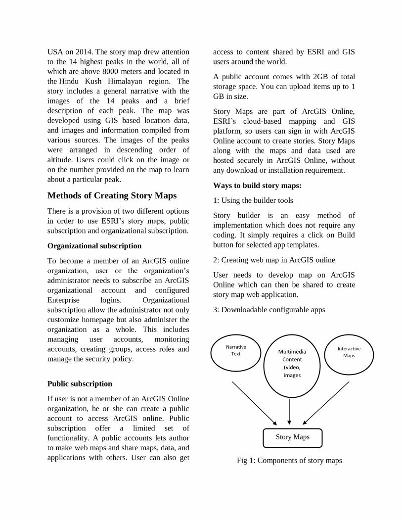
USA on 2014. The story map drew attention
to the 14 highest peaks in the world, all of
which are above 8000 meters and located in
the Hindu Kush Himalayan region. The
story includes a general narrative with the
images of the 14 peaks and a brief
description of each peak. The map was
developed using GIS based location data,
and images and information compiled from
various sources. The images of the peaks
were arranged in descending order of
altitude. Users could click on the image or
on the number provided on the map to learn
about a particular peak.
Methods of Creating Story Maps
There is a provision of two different options
in order to use ESRI’s story maps, public
subscription and organizational subscription.
Organizational subscription
To become a member of an ArcGIS online
organization, user or the organization’s
administrator needs to subscribe an ArcGIS
organizational account and configured
Enterprise logins. Organizational
subscription allow the administrator not only
customize homepage but also administer the
organization as a whole. This includes
managing user accounts, monitoring
accounts, creating groups, access roles and
manage the security policy.
Public subscription
If user is not a member of an ArcGIS Online
organization, he or she can create a public
account to access ArcGIS online. Public
subscription offer a limited set of
functionality. A public accounts lets author
to make web maps and share maps, data, and
applications with others. User can also get
access to content shared by ESRI and GIS
users around the world.
A public account comes with 2GB of total
storage space. You can upload items up to 1
GB in size.
Story Maps are part of ArcGIS Online,
ESRI’s cloud-based mapping and GIS
platform, so users can sign in with ArcGIS
Online account to create stories. Story Maps
along with the maps and data used are
hosted securely in ArcGIS Online, without
any download or installation requirement.
Ways to build story maps:
1: Using the builder tools
Story builder is an easy method of
implementation which does not require any
coding. It simply requires a click on Build
button for selected app templates.
2: Creating web map in ArcGIS online
User needs to develop map on ArcGIS
Online which can then be shared to create
story map web application.
3: Downloadable configurable apps
Fig 1: Components of story maps
Story Maps
Interactive
Maps Multimedia
Content
(video,
images
Narrative
Text
Result and Discussion
Story Maps have been used as a
convenient and efficient means of
communication at ICIMOD for the past
couple of years, and its application is
increasingly becoming adoptive in the
organization. The simplicity of its use is
the biggest advantage, thus, enabling the
possibilities of its inclusion in several
sectors of Nepal. Short and concise text
assists reading and understanding. This
approach is required as people have
limited attentional resources. Maps
support the understanding of natural
disaster issues spatially and allow user to
interact with the Story Map resource.
This is likely to improve retention of
information. Story Maps’ in-built
interactivity is very important and
enables individuals to engage with the
resource. For example, asking those at
risk to identify their homes and level of
risk could be a useful engagement
exercise. Using a balanced mixed media
approach, to communicate hazard and
risk information is important and helps
alleviate information overload. It also
potentially supports multi-sensory
learning, which has associated benefits.
There are several geographically
challenged touristic areas in Nepal
whose information is not available
online. For all such locations, creating a
story map helps to make the information
available in an interactive way to
visitors. This also enables them to
strategically plan the visit and stay.
Similarly, an illustration of potentially
vulnerable areas of the nation can greatly
minimize the impact of various natural
casualties, addressing the lack of
effective risk communication through
story maps. For educational purposes, an
instructional interaction with students
help to foster effective teaching-learning
environment. It further enhances
student’s ability to interact with map and
allows to explore spatial patterns and
trends which leads to understanding
about the true nature of a geographic
phenomenon. The story map can be a
brainstorming tool for government to
create spaces and opportunities for
communication, participation and
knowledge sharing.
One of the challenges is achieving a high
quality digital product using the web as
medium. Nevertheless, current web
mapping technology provide the means
to develop high quality thematic map
and base map and research in web map
cartography. The story map can be
updated more frequently and cost-
effectively through electronic
publication rather than paper
publication, and links to more materials
can be incorporated.
Conclusion
The goal of this study is to suggest how
story maps can be best utilized in
various potential domains in the context
of Nepal. There are several potential
areas including, but not limited to,
education, tourism, natural disaster and
government, in Nepal, which can highly
benefit by the use of Story Maps. The
effectiveness of this technology within a
critical GIS framework can be
understood, evaluated and discussed by
both non-users and users of it. Involving
students actively in the process of
creating storytelling with maps can spark
their creativity by thinking and telling
their own stories. Storytelling with maps
is an opportunity to promote imagination
to solve problem and think beyond
normal boundaries. Interactive atlas
provides for a more engaging,
interactive, and exploratory environment
for government. Last but not the least,
accurate location information
presentation in a graphical way can
enhance user’s capability of navigation
and can thus be an effective means of
communication.
References
ESRI. 2018. The five principles of effective
storytelling. ESRI, Redlands, CA.
https://storymaps.arcgis.com/en/five-
principles/(Accessed 3 Dec. 2018).
ESRI. 2018. How to Make a Story Map.
ESRI, Redlands, CA.
https://storymaps.arcgis.com/en/how-
to/(Accessed 3 Dec. 2018).
Marta, M., & Osso, P. (2015). Story Maps at
school: teaching and learning stories with
maps. J-Reading - Journal Of Research And
Didactics In Geography, 0(2). Retrieved
from http://www.j-
reading.org/index.php/geography/article/vie
w/116
Berendsen, M.E.; Hamerlinck, J.D.;
Webster, G.R. Digital Story Mapping to
Advance Educational Atlas Design and
Enable Student Engagement. ISPRS Int. J.
Geo-Inf. 2018, 7, 125.
Cope, M. P., E. A. Mikhailova, C. J. Post,
M. A. Schlautman, and P. Carbajales-Dale.
2018. Developing and Evaluating an ESRI
Story Map as an Educational Tool. Natural
Sciences Education 47:180008.
doi:10.4195/nse2018.04.0008
Austin, Brittany Grace, "Investigating the
Influence of Esri Story Map Design on
Partcipation in Sustainability-Related
Activities" (2018). Masters Theses &
Specialist Projects. Paper 2571.
https://digitalcommons.wku.edu/theses/2571
Baker, T. R. (2005). Internet-based mapping
to support K12 education. The Professional
Geographer, 57(1), 44–50.
Graves, Mallory Elizabeth.Spatial narratives
of struggle and activism in
the Del Amo and Montrose Superfund clean
ups: a community-
engaged Web GIS story map.
http://digitallibrary.usc.edu/cdm/ref/collectio
n/p15799coll3/id/597488
Sébastien Caquard & William
Cartwright (2014) Narrative Cartography:
From Mapping Stories to the Narrative of
Maps and Mapping, The Cartographic
Journal, 51:2, 101-
106, DOI: 10.1179/0008704114Z.00000000
0130
ISPRS International Journal of Geo-
Information 2018, 7(3), 125;
doi:10.3390/ijgi7030125

Information and Communication Technology Challenges for Digital Tourism Business Model for Nepal
Deepanjal Shrestha1, Niranjan Khakurel2, Tan Wenan3 13
School of Computer Science and Technology Nanjing University of Aeronautics and Astronautics, Nanjing 210016, China
2Nepal College of Information Technology
Pokhara University, Pokhara, Nepal
Email: [email protected], [email protected] , [email protected]
Abstract: Information and Communication Technology has
created a huge impact on the business models. It has changed
the way business was done few years ago, redefining business
in the light of digital technologies. Tourism is one such vital
industry that finds enormous application of Information and
Communication Technology on it, changing the entire value
chain from tourism creation and marketing to distribution and
consumption. Tourism is one of the biggest industries of
Nepal and the government of Nepal has targeted this industry
as a prime source for economic development. Nepal
government has identified that the role of ICT is vital for the
growth and development of Tourism. Besides a lot of
technological development and innovation in global tourism
industry, Nepal is unable to attain benefits from the
application of Information and Communication Technology.
In our study we have examined the factors that are responsible
for poor implementation of ICT in Tourism industry of Nepal.
We employ qualitative exploratory method based on
interviews, structured and semi structured questionnaires to
accomplish the study. The study contributes in finding the
factors responsible for poor implementation of ICT and
analyzes the challenges regarding its implementation. Further,
the findings are elaborated to build a conceptual framework
for Digital Tourism Business Model for Nepal.
Keywords: ICT, Tourism Industry, Digital Business Systems,
Tourism Model.
I. BACKGROUND
Tourism has grown as an industry worldwide in the last two
and half decades and has outshined traditional industries to
become one of the world's largest and fastest growing
economic activities [4] [5]. Scholars have found that there is a
huge transition in Tourism industry in the current times due to
penetration of Information and Communication Technology
[5]. The use of ICT to promote tourism and overcome
geographical challenges has become particularly important.
The application of ICT is the most important aspect for a
successful tourism economy [1][5][6] as the whole industry
relies on correct and timely information. ICT plays a vital role
as an information carrier in case of emergency situations,
changing climatic conditions and other sensitive aspects. Thus
ICT serves as a backbone for this industry integrating the
beneficiaries, the service providers and product sectors [11],
making it as a solid chain of interdependent components.
ICT is a boon for the under developed countries like Nepal
and it can serve in many aspects to gain advantage in business,
governance or other sectors. Nepal heavily relies on Tourism
and it has become a leading economic activity. Tourism
Industry is a main contributor in GDP of Nepal and generating
huge employment. The government of Nepal has realized
that in order to grow economically and generate employment
opportunities, it must focus on the Tourism Industry.
Moreover, it has also realized the importance of ICT in
Tourism Sector. There are many plans and policies initiated by
the government to take advantage of the global information
network and increase the national and the international
competitiveness in Tourism industry. Despite this vision a
little or marginal progress is made and there has been no
recent research focusing on understanding ICT usage in the
tourism sector. This work argues that due to the lack of
research in this area, ICT application in the tourism industry
needs a deeper investigation. Thus, this study aims to analyze
the current ICT infrastructure of Nepal and highlight the
challenges that are seen in the adoption and integration of ICT.
Further a broader conceptual model for Digital Tourism
Business Model for Nepal is also discussed.
II. LITERATURE REVIEW
Studies on ICT use in the tourism industry have shown that
the use of ICT is not only a vital component of the tourism
industry, but that ICT will continue to be crucial tool,
especially for developing countries (UNCTAD, 2005). The
adoption of Computer Reservation System (CRS) in airlines in
1950s and the transformation to Global Distribution Systems
(GDSs) in the 1980‟s, Hotel property management systems
and hotel CRS systems later, are some on the oldest
application of ICT in tourism [9][10]. The birth of Internet
brought a revolutionary changes to the structure of this
industry by letting the service providers sell their products and
services directly [9][10][11]. There are new models in practice
which threatened the intermediaries worrying them of being
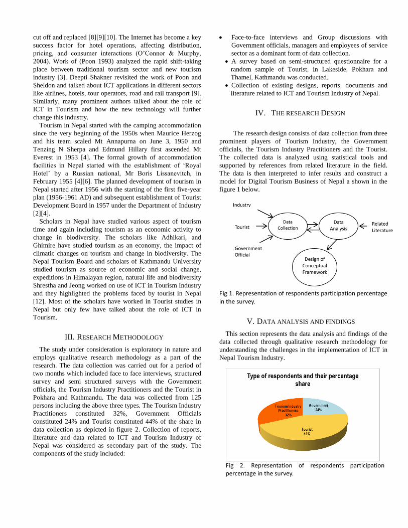
cut off and replaced [8][9][10]. The Internet has become a key
success factor for hotel operations, affecting distribution,
pricing, and consumer interactions (O‟Connor & Murphy,
2004). Work of (Poon 1993) analyzed the rapid shift-taking
place between traditional tourism sector and new tourism
industry [3]. Deepti Shakner revisited the work of Poon and
Sheldon and talked about ICT applications in different sectors
like airlines, hotels, tour operators, road and rail transport [9].
Similarly, many prominent authors talked about the role of
ICT in Tourism and how the new technology will further
change this industry.
Tourism in Nepal started with the camping accommodation
since the very beginning of the 1950s when Maurice Herzog
and his team scaled Mt Annapurna on June 3, 1950 and
Tenzing N Sherpa and Edmund Hillary first ascended Mt
Everest in 1953 [4]. The formal growth of accommodation
facilities in Nepal started with the establishment of „Royal
Hotel‟ by a Russian national, Mr Boris Lissanevitch, in
February 1955 [4][6]. The planned development of tourism in
Nepal started after 1956 with the starting of the first five-year
plan (1956-1961 AD) and subsequent establishment of Tourist
Development Board in 1957 under the Department of Industry
[2][4].
Scholars in Nepal have studied various aspect of tourism
time and again including tourism as an economic activity to
change in biodiversity. The scholars like Adhikari, and
Ghimire have studied tourism as an economy, the impact of
climatic changes on tourism and change in biodiversity. The
Nepal Tourism Board and scholars of Kathmandu University
studied tourism as source of economic and social change,
expeditions in Himalayan region, natural life and biodiversity
Shrestha and Jeong worked on use of ICT in Tourism Industry
and they highlighted the problems faced by tourist in Nepal
[12]. Most of the scholars have worked in Tourist studies in
Nepal but only few have talked about the role of ICT in
Tourism.
III. RESEARCH METHODOLOGY
The study under consideration is exploratory in nature and
employs qualitative research methodology as a part of the
research. The data collection was carried out for a period of
two months which included face to face interviews, structured
survey and semi structured surveys with the Government
officials, the Tourism Industry Practitioners and the Tourist in
Pokhara and Kathmandu. The data was collected from 125
persons including the above three types. The Tourism Industry
Practitioners constituted 32%, Government Officials
constituted 24% and Tourist constituted 44% of the share in
data collection as depicted in figure 2. Collection of reports,
literature and data related to ICT and Tourism Industry of
Nepal was considered as secondary part of the study. The
components of the study included:
Face-to-face interviews and Group discussions with
Government officials, managers and employees of service
sector as a dominant form of data collection.
A survey based on semi-structured questionnaire for a
random sample of Tourist, in Lakeside, Pokhara and
Thamel, Kathmandu was conducted.
Collection of existing designs, reports, documents and
literature related to ICT and Tourism Industry of Nepal.
IV. THE RESEARCH DESIGN
The research design consists of data collection from three
prominent players of Tourism Industry, the Government
officials, the Tourism Industry Practitioners and the Tourist.
The collected data is analyzed using statistical tools and
supported by references from related literature in the field.
The data is then interpreted to infer results and construct a
model for Digital Tourism Business of Nepal a shown in the
figure 1 below.
Fig 1. Representation of respondents participation percentage in the survey.
V. DATA ANALYSIS AND FINDINGS
This section represents the data analysis and findings of the
data collected through qualitative research methodology for
understanding the challenges in the implementation of ICT in
Nepal Tourism Industry.
Data Collection
Data Analysis
Design of Conceptual Framework
Tourist
Industry Players
Government Official
Related Literature
Fig 2. Representation of respondents participation percentage in the survey.
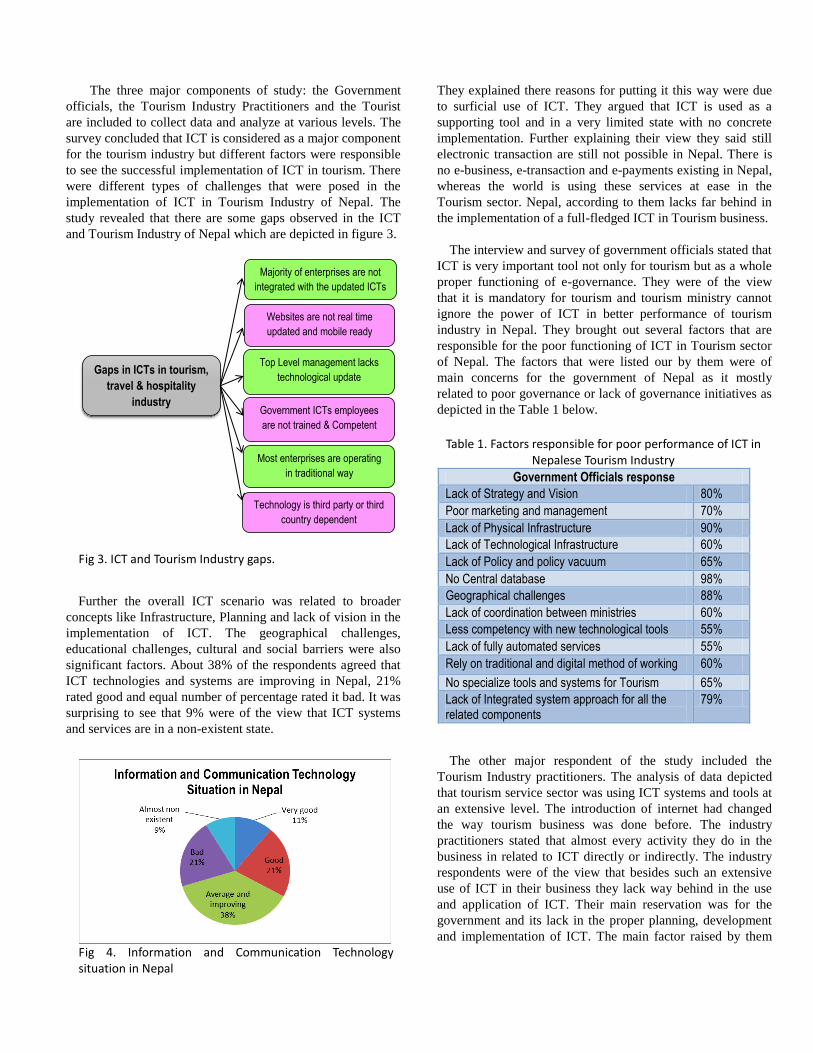
The three major components of study: the Government
officials, the Tourism Industry Practitioners and the Tourist
are included to collect data and analyze at various levels. The
survey concluded that ICT is considered as a major component
for the tourism industry but different factors were responsible
to see the successful implementation of ICT in tourism. There
were different types of challenges that were posed in the
implementation of ICT in Tourism Industry of Nepal. The
study revealed that there are some gaps observed in the ICT
and Tourism Industry of Nepal which are depicted in figure 3.
Further the overall ICT scenario was related to broader
concepts like Infrastructure, Planning and lack of vision in the
implementation of ICT. The geographical challenges,
educational challenges, cultural and social barriers were also
significant factors. About 38% of the respondents agreed that
ICT technologies and systems are improving in Nepal, 21%
rated good and equal number of percentage rated it bad. It was
surprising to see that 9% were of the view that ICT systems
and services are in a non-existent state.
They explained there reasons for putting it this way were due
to surficial use of ICT. They argued that ICT is used as a
supporting tool and in a very limited state with no concrete
implementation. Further explaining their view they said still
electronic transaction are still not possible in Nepal. There is
no e-business, e-transaction and e-payments existing in Nepal,
whereas the world is using these services at ease in the
Tourism sector. Nepal, according to them lacks far behind in
the implementation of a full-fledged ICT in Tourism business.
The interview and survey of government officials stated that
ICT is very important tool not only for tourism but as a whole
proper functioning of e-governance. They were of the view
that it is mandatory for tourism and tourism ministry cannot
ignore the power of ICT in better performance of tourism
industry in Nepal. They brought out several factors that are
responsible for the poor functioning of ICT in Tourism sector
of Nepal. The factors that were listed our by them were of
main concerns for the government of Nepal as it mostly
related to poor governance or lack of governance initiatives as
depicted in the Table 1 below.
The other major respondent of the study included the
Tourism Industry practitioners. The analysis of data depicted
that tourism service sector was using ICT systems and tools at
an extensive level. The introduction of internet had changed
the way tourism business was done before. The industry
practitioners stated that almost every activity they do in the
business in related to ICT directly or indirectly. The industry
respondents were of the view that besides such an extensive
use of ICT in their business they lack way behind in the use
and application of ICT. Their main reservation was for the
government and its lack in the proper planning, development
and implementation of ICT. The main factor raised by them Fig 4. Information and Communication Technology situation in Nepal
Websites are not real time
updated and mobile ready
Top Level management lacks
technological update
Government ICTs employees
are not trained & Competent
Most enterprises are operating
in traditional way
Technology is third party or third
country dependent
Majority of enterprises are not
integrated with the updated ICTs
Gaps in ICTs in tourism,
travel & hospitality
industry
Fig 3. ICT and Tourism Industry gaps.
Table 1. Factors responsible for poor performance of ICT in Nepalese Tourism Industry
Government Officials response
Lack of Strategy and Vision 80%
Poor marketing and management 70%
Lack of Physical Infrastructure 90%
Lack of Technological Infrastructure 60%
Lack of Policy and policy vacuum 65%
No Central database 98%
Geographical challenges 88%
Lack of coordination between ministries 60%
Less competency with new technological tools 55%
Lack of fully automated services 55%
Rely on traditional and digital method of working 60%
No specialize tools and systems for Tourism 65%
Lack of Integrated system approach for all the related components
79%
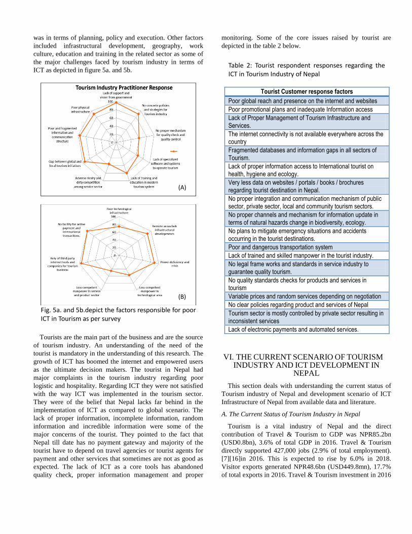
was in terms of planning, policy and execution. Other factors
included infrastructural development, geography, work
culture, education and training in the related sector as some of
the major challenges faced by tourism industry in terms of
ICT as depicted in figure 5a. and 5b.
Tourists are the main part of the business and are the source
of tourism industry. An understanding of the need of the
tourist is mandatory in the understanding of this research. The
growth of ICT has boomed the internet and empowered users
as the ultimate decision makers. The tourist in Nepal had
major complaints in the tourism industry regarding poor
logistic and hospitality. Regarding ICT they were not satisfied
with the way ICT was implemented in the tourism sector.
They were of the belief that Nepal lacks far behind in the
implementation of ICT as compared to global scenario. The
lack of proper information, incomplete information, random
information and incredible information were some of the
major concerns of the tourist. They pointed to the fact that
Nepal till date has no payment gateway and majority of the
tourist have to depend on travel agencies or tourist agents for
payment and other services that sometimes are not as good as
expected. The lack of ICT as a core tools has abandoned
quality check, proper information management and proper
monitoring. Some of the core issues raised by tourist are
depicted in the table 2 below.
VI. THE CURRENT SCENARIO OF TOURISM
INDUSTRY AND ICT DEVELOPMENT IN
NEPAL
This section deals with understanding the current status of
Tourism industry of Nepal and development scenario of ICT
Infrastructure of Nepal from available data and literature.
A. The Current Status of Tourism Industry in Nepal
Tourism is a vital industry of Nepal and the direct
contribution of Travel & Tourism to GDP was NPR85.2bn
(USD0.8bn), 3.6% of total GDP in 2016. Travel & Tourism
directly supported 427,000 jobs (2.9% of total employment).
[7][16]in 2016. This is expected to rise by 6.0% in 2018.
Visitor exports generated NPR48.6bn (USD449.8mn), 17.7%
of total exports in 2016. Travel & Tourism investment in 2016
Fig. 5a. and 5b.depict the factors responsible for poor ICT in Tourism as per survey
(A)
(B)
Table 2: Tourist respondent responses regarding the ICT in Tourism Industry of Nepal
Tourist Customer response factors
Poor global reach and presence on the internet and websites
Poor promotional plans and inadequate Information access
Lack of Proper Management of Tourism Infrastructure and Services.
The internet connectivity is not available everywhere across the country
Fragmented databases and information gaps in all sectors of Tourism.
Lack of proper information access to International tourist on health, hygiene and ecology.
Very less data on websites / portals / books / brochures regarding tourist destination in Nepal.
No proper integration and communication mechanism of public sector, private sector, local and community tourism sectors.
No proper channels and mechanism for information update in terms of natural hazards change in biodiversity, ecology.
No plans to mitigate emergency situations and accidents occurring in the tourist destinations.
Poor and dangerous transportation system
Lack of trained and skilled manpower in the tourist industry.
No legal frame works and standards in service industry to guarantee quality tourism.
No quality standards checks for products and services in tourism
Variable prices and random services depending on negotiation
No clear policies regarding product and services of Nepal
Tourism sector is mostly controlled by private sector resulting in inconsistent services
Lack of electronic payments and automated services.
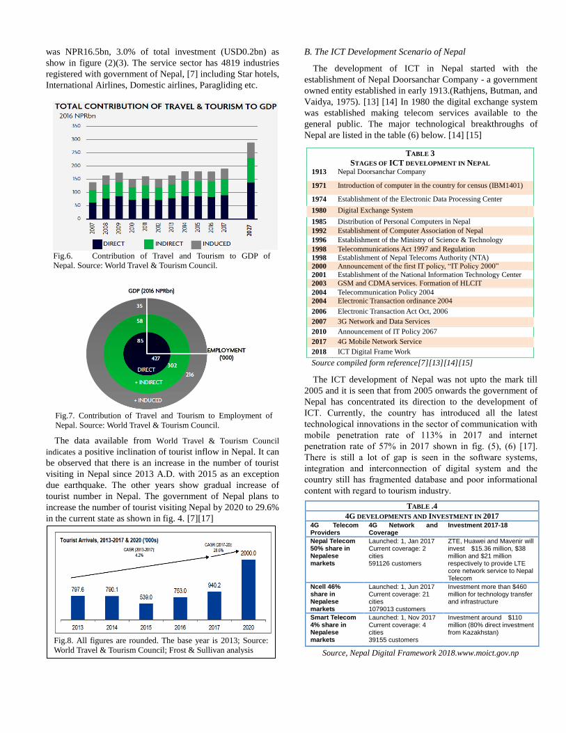
was NPR16.5bn, 3.0% of total investment (USD0.2bn) as
show in figure (2)(3). The service sector has 4819 industries
registered with government of Nepal, [7] including Star hotels,
International Airlines, Domestic airlines, Paragliding etc.
The data available from World Travel & Tourism Council
indicates a positive inclination of tourist inflow in Nepal. It can
be observed that there is an increase in the number of tourist
visiting in Nepal since 2013 A.D. with 2015 as an exception
due earthquake. The other years show gradual increase of
tourist number in Nepal. The government of Nepal plans to
increase the number of tourist visiting Nepal by 2020 to 29.6%
in the current state as shown in fig. 4. [7][17]
B. The ICT Development Scenario of Nepal
The development of ICT in Nepal started with the
establishment of Nepal Doorsanchar Company - a government
owned entity established in early 1913.(Rathjens, Butman, and
Vaidya, 1975). [13] [14] In 1980 the digital exchange system
was established making telecom services available to the
general public. The major technological breakthroughs of
Nepal are listed in the table (6) below. [14] [15]
The ICT development of Nepal was not upto the mark till
2005 and it is seen that from 2005 onwards the government of
Nepal has concentrated its direction to the development of
ICT. Currently, the country has introduced all the latest
technological innovations in the sector of communication with
mobile penetration rate of 113% in 2017 and internet
penetration rate of 57% in 2017 shown in fig. (5), (6) [17].
There is still a lot of gap is seen in the software systems,
integration and interconnection of digital system and the
country still has fragmented database and poor informational
content with regard to tourism industry.
Fig.6. Contribution of Travel and Tourism to GDP of
Nepal. Source: World Travel & Tourism Council.
Fig.7. Contribution of Travel and Tourism to Employment of
Nepal. Source: World Travel & Tourism Council.
Fig.8. All figures are rounded. The base year is 2013; Source:
World Travel & Tourism Council; Frost & Sullivan analysis
TABLE 3
STAGES OF ICT DEVELOPMENT IN NEPAL 1913 Nepal Doorsanchar Company
1971 Introduction of computer in the country for census (IBM1401)
1974 Establishment of the Electronic Data Processing Center
1980 Digital Exchange System
1985 Distribution of Personal Computers in Nepal
1992 Establishment of Computer Association of Nepal
1996 Establishment of the Ministry of Science & Technology
1998 Telecommunications Act 1997 and Regulation
1998 Establishment of Nepal Telecoms Authority (NTA)
2000 Announcement of the first IT policy, “IT Policy 2000”
2001 Establishment of the National Information Technology Center
2003 GSM and CDMA services. Formation of HLCIT
2004 Telecommunication Policy 2004
2004 Electronic Transaction ordinance 2004
2006 Electronic Transaction Act Oct, 2006
2007 3G Network and Data Services
2010 Announcement of IT Policy 2067
2017 4G Mobile Network Service
2018 ICT Digital Frame Work
Source compiled form reference[7][13][14][15]
TABLE .4
4G DEVELOPMENTS AND INVESTMENT IN 2017 4G Telecom Providers
4G Network and Coverage
Investment 2017-18
Nepal Telecom 50% share in Nepalese markets
Launched: 1, Jan 2017 Current coverage: 2 cities 591126 customers
ZTE, Huawei and Mavenir will invest $15.36 million, $38 million and $21 million respectively to provide LTE core network service to Nepal Telecom
Ncell 46% share in Nepalese markets
Launched: 1, Jun 2017 Current coverage: 21 cities 1079013 customers
Investment more than $460 million for technology transfer and infrastructure
Smart Telecom 4% share in Nepalese markets
Launched: 1, Nov 2017 Current coverage: 4 cities 39155 customers
Investment around $110 million (80% direct investment from Kazakhstan)
Source, Nepal Digital Framework 2018.www.moict.gov.np
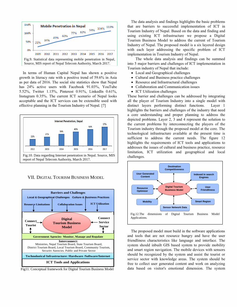
In terms of Human Capital Nepal has shown a positive
growth in literacy rate with a positive trend of 59.6% in Asia
as per data of 2016. The social site statistics show that Nepal
has 24% active users with Facebook 91.03%, YouTube
5.52%, Twitter 1.15%, Pinterest 0.91%, LinkedIn 0.61%,
Instagram 0.35%. The current ICT scenario of Nepal looks
acceptable and the ICT services can be extensible used with
effective planning in the Tourism Industry of Nepal. [7]
VII. DIGITAL TOURISM BUSINESS MODEL
The data analysis and findings highlights the basic problems
that are barriers to successful implementation of ICT in
Tourism Industry of Nepal. Based on the data and finding and
using existing ICT infrastructure we propose a Digital
Tourism Business Model to address the current of Tourism
Industry of Nepal. The proposed model is a six layered design
with each layer addressing the specific problem of ICT
implementation in Tourism Industry of Nepal.
The whole data analysis and findings can be summed
into 5 major barriers and challenges of ICT implementation in
Tourism industry of Nepal that include:
Local and Geographical challenges
Cultural and Business practice challenges
Resource and Infrastructural challenges
Collaboration and Communication issues
ICT Utilization challenges
These barrier and challenges can be addressed by integrating
all the player of Tourism Industry into a single model with
distinct layers performing distinct functions. Layer 1
highlights the barriers and challenges of the industry that need
a core understanding and proper planning to address the
depicted problems. Layer 2, 3 and 4 represent the solution to
the current problems by interconnecting the players of the
Tourism industry through the proposed model at the core. The
technological infrastructure available at the present time is
sufficient to address the current needs. The figure 12
highlights the requirements of ICT tools and applications to
addresses the issues of cultural and business practice, resource
limitation, ICT utilization and geographical and local
challenges.
The proposed model must build in the software applications
and tools that are not resource hungry and have the user
friendliness characteristics like language and interface. The
system should inbuilt GIS based system to provide mobility
and smart region navigation. The mobile devices with sensors
should be recognized by the system and assist the tourist or
service sector with knowledge areas. The system should be
free to collect user generated content and work on analyzing
data based on visitor's emotional dimension. The system
Fig.9. Statistical data representing mobile penetration in Nepal,
Source, MIS report of Nepal Telecom Authority, March 2017.
Fig.10. Data regarding Internet penetration in Nepal. Source, MIS
report of Nepal Telecom Authority, March 2017.
Digital Tourism
Business Model
Mobility Smart Region
User Generated
Content Indexed in search
Engines
Sensor Network Data
Destination
Competitiveness
Resource
Optimizer
User
Friendliness
Fig.12.The dimensions of Digital Tourism Business Model
Applications.
Resource Limitations
Local & Geographical Challenges
Collaboration Issues
Culture & Business Practices
ICT Utilization
Interconnect:
Government Agencies- Monitor, Manage and Regulate
Digital
Tourism Business
Model
Connect
Tourist
Connect
Service
Sector
Ministries, Nepal Tourism Board, State Tourism Board,
District Tourism Board, Local Tourism Board, Community Tourism,
Security Agencies, Public and Private Sector
ICT Tools and Applications
Technological Infrastructure: Hardware /Software/Internet
Barriers and Challenges
Fig11. Conceptual framework for Digital Tourism Business Model
. The proposed design of Digital Tourism Business Model
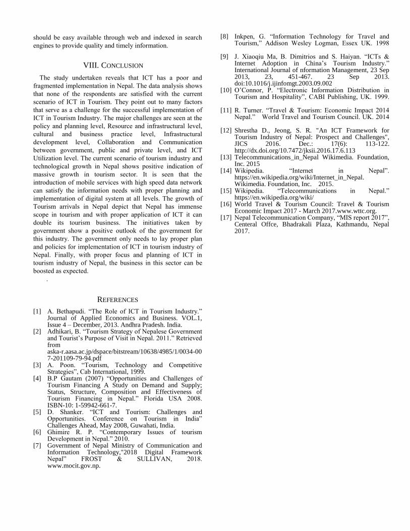
should be easy available through web and indexed in search
engines to provide quality and timely information.
VIII. CONCLUSION
The study undertaken reveals that ICT has a poor and
fragmented implementation in Nepal. The data analysis shows
that none of the respondents are satisfied with the current
scenario of ICT in Tourism. They point out to many factors
that serve as a challenge for the successful implementation of
ICT in Tourism Industry. The major challenges are seen at the
policy and planning level, Resource and infrastructural level,
cultural and business practice level, Infrastructural
development level, Collaboration and Communication
between government, public and private level, and ICT
Utilization level. The current scenario of tourism industry and
technological growth in Nepal shows positive indication of
massive growth in tourism sector. It is seen that the
introduction of mobile services with high speed data network
can satisfy the information needs with proper planning and
implementation of digital system at all levels. The growth of
Tourism arrivals in Nepal depict that Nepal has immense
scope in tourism and with proper application of ICT it can
double its tourism business. The initiatives taken by
government show a positive outlook of the government for
this industry. The government only needs to lay proper plan
and policies for implementation of ICT in tourism industry of
Nepal. Finally, with proper focus and planning of ICT in
tourism industry of Nepal, the business in this sector can be
boosted as expected.
.
REFERENCES
[1] A. Bethapudi. “The Role of ICT in Tourism Industry.” Journal of Applied Economics and Business. VOL.1, Issue 4 – December, 2013. Andhra Pradesh. India.
[2] Adhikari, B. “Tourism Strategy of Nepalese Government and Tourist‟s Purpose of Visit in Nepal. 2011.” Retrieved from aska-r.aasa.ac.jp/dspace/bitstream/10638/4985/1/0034-007-201109-79-94.pdf
[3] A. Poon. “Tourism, Technology and Competitive Strategies”, Cab International, 1999.
[4] B.P Gautam (2007) “Opportunities and Challenges of Tourism Financing A Study on Demand and Supply; Status, Structure, Composition and Effectiveness of Tourism Financing in Nepal.” Florida USA 2008. ISBN-10: 1-59942-661-7.
[5] D. Shanker. “ICT and Tourism: Challenges and Opportunities. Conference on Tourism in India” Challenges Ahead, May 2008, Guwahati, India.
[6] Ghimire R. P. “Contemporary Issues of tourism Development in Nepal.” 2010.
[7] Government of Nepal Ministry of Communication and Information Technology,"2018 Digital Framework Nepal” FROST & SULLIVAN, 2018. www.mocit.gov.np.
[8] Inkpen, G. “Information Technology for Travel and Tourism,” Addison Wesley Logman, Essex UK. 1998
[9] J. Xiaoqiu Ma, B. Dimitrios and S. Haiyan. “ICTs & Internet Adoption in China‟s Tourism Industry.” International Journal of nformation Management, 23 Sep 2013, 23, 451-467. 23 Sep 2013. doi:10.1016/j.ijinfomgt.2003.09.002
[10] O‟Connor, P. “Electronic Information Distribution in Tourism and Hospitality”, CABI Publishing, UK. 1999.
[11] R. Turner. “Travel & Tourism: Economic Impact 2014 Nepal.” World Travel and Tourism Council. UK. 2014
[12] Shrestha D., Jeong, S. R. "An ICT Framework for Tourism Industry of Nepal: Prospect and Challenges", JICS 2016. Dec.: 17(6): 113-122. http://dx.doi.org/10.7472/jksii.2016.17.6.113
[13] Telecommunications_in_Nepal Wikimedia. Foundation, Inc. 2015
[14] Wikipedia. “Internet in Nepal”. https://en.wikipedia.org/wiki/Internet_in_Nepal. Wikimedia. Foundation, Inc. 2015.
[15] Wikipedia. “Telecommunications in Nepal.” https://en.wikipedia.org/wiki/
[16] World Travel & Tourism Council: Travel & Tourism Economic Impact 2017 - March 2017.www.wttc.org.
[17] Nepal Telecommunication Company, “MIS report 2017”, Centeral Offce, Bhadrakali Plaza, Kathmandu, Nepal 2017.

Context-Aware Privacy Preservation Approaches on
Location Based Services using Recurrent Neural
Network
Ramu Pandey
Nepal Collge of Information
Technology
Kathmandu,Nepal
Roshan Chitrakar
Nepal College of Information
Technology
Kathmandu,Nepal
Abstract— With the widespread proliferation of usage of social
networks, smartphones and smartphone apps, privacy
preservation has become an important issue. This has led to
increased concerns about the privacy of the underlying data.
Various social media, mobile devices and sensors are
collecting huge amount of data daily and analyzing them for
business purpose or designing more convenience systems.
But on the run, privacy of people has been on threat. Service
providers might have chance to misuse the individuals
private information. On the other side, facilitating people for
making their lifestyles easier and automated systems can be
more expecting. Thus, data mining by preserving the
privacy can be the best way. The existing privacy
preservation approaches for smartphones usually are less
efficient due to the lack of consideration of active defense
policies and temporal correlations between contexts related
to users. Among various types of data collected according to
various contexts, the privacy of trajectory data collected by
Location Based Services (LBS) is also very important
according to contexts for various persons and groups. In this
paper, through modelling the trajectory data and the
temporal correlations among contexts, we present an
efficient approach that preserves the privacy of location data
of users from adversaries dynamically on the basis of the
sensitivity of user’s context. Our efficient approach adopts
active defense policy and decides how to release the current
location information and contexts of a user to maximize the
level of Quality of Services (QoS) of context-aware apps
and services with privacy preservation. To make our
approach more efficient and robust, and increase privacy
involving long-term dependency we have used Recurrent
Neural Network (RNN) model irrespective of the traditional
Markov Chain model to model the trajectory data and
contexts and their temporal correlations. Further, we have
adopted the “release and deceive” policy and implemented a
special kind of RNN i.e. Long-Short-Term-Memory
(LSTM) and treated sensitive contexts as exceptions to
preserve the sensitive contexts. We have conducted the
extensive simulations on real datasets and compared the
performance of our algorithm and approach with previous
approaches on the basis of privacy, performance and utility
of data.
Keywords— Context-Aware Privacy Preservation, Data
Mining, Location Based Services, Recurrent Neural Network
I. INTRODUCTION
Nowadays, smartphones have been greatly proliferated and smartphone applications (apps) and social networking sites have been widely developed. Specifically, context-aware apps greatly facilitate people as context-aware personalized services related to people’ contexts have been provided. In fact, a variety of sensors (e.g. GPS, microphone, accelerometers, magnetometer, light, and proximity) embedded in smartphones have the capability to measure the surroundings and the status related to the smartphone owner and then provide related data to context-aware apps. The sensory data can be exploited to infer the context or the status about a user. For example, the location information of a user can be reported by GPS data, the transportation state (e.g., walking, running, or standing) can be evaluated by the accelerometers, and the voice and scene can be recorded by microphone and camera, respectively. Furthermore, the inferred context can be further analyzed by context-aware apps for providing context-aware personalized services. Examples of such applications include GeoReminder that notifies the user when he is at a particular location, JogBuddy that monitors how much he jogs in a day, PhoneWise that automatically mutes the phone during meetings, SocialGroupon that delivers coupons or recommendations when he is in a group of friends, etc.
However, these context-aware mobile applications raise serious privacy concerns. Today, people already believe that risks of sharing location information outweigh the benefits in many location based services [12]. One reason why risks are high is that many mobile applications today aggressively collect much more personal context data than what is needed to provide their functionalities [13] (for example, a calculator application might send the user’s location to an advertisement server). Moreover, applications rarely provide privacy policies that clearly state how users’ sensitive information will be used, and with what third-parties it will be shared. To avoid the risks, a user can decide not to install these application or not to release any context information to them (by explicitly turning off sensors); but then the user might not be able to enjoy the utility provided by these applications. In order to explore a better tradeoff between privacy and utility, we can let the user control at a fine granularity when and what context data is shared with which application [14, 15]. For example, a user might be okay to release when he is at lunch but he might be hesitant to release when he is at a hospital. With such fine-grained decisions, a user can choose a point in the privacy-utility tradeoff for an application and can still enjoy its full functionality when he chooses to release his context
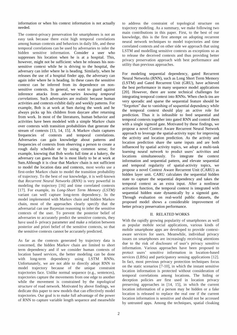
2
information or when his context information is not actually needed.
The context-privacy preservation for smartphones is not an
easy task because there exist high temporal correlations
among human contexts and behaviors in daily life, and these
temporal correlations can be used by adversaries to infer the
hidden sensitive information. Consider a user who
suppresses his location when he is at a hospital. This,
however, might not be sufficient: when he releases his non-
sensitive context while he is driving to the hospital, the
adversary can infer where he is heading. Similarly, when he
releases the use of a hospital finder app, the adversary can
again infer where he is heading. In these cases the sensitive
context can be inferred from its dependence on non-
sensitive contexts. In general, we want to guard against
inference attacks from adversaries knowing temporal
correlations. Such adversaries are realistic because human
activities and contexts exhibit daily and weekly patterns. For
example, Bob is at work at 9am during the week and he
always picks up his children from daycare after returning
from work. In most of the literatures, human behavior and
activities have been modeled with a simple Markov chain
over contexts with transition probabilities that generate the
stream of contexts [13, 14, 15]. A Markov chain captures
frequencies of contexts and temporal correlations.
Adversaries can gain knowledge about patterns and
frequencies of contexts from observing a person to create a
rough daily schedule or by using common sense; for
example, knowing that Bob works full time at a bakery, the
adversary can guess that he is most likely to be at work at
9am.Although it is clear that Markov chain is not sufficient
to model the location data and contexts, most works use a
first-order Markov chain to model the transition probability
of trajectory. To the best of our knowledge, it is well-known
that Recurrent Neural Networks (RNN) is very powerful in
modeling the trajectory [16] and time correlated contexts
[17]. For example, its Long-Short Term Memory (LSTM)
variant can well capture long-term dependency. In the
model implemented with Markov chain and hidden Markov
chain, most of the approaches clearly specify that the
adversarial can use Bayesian reasoning to infer the sensitive
contexts of the user. To prevent the posterior belief of
adversaries to accurately predict the sensitive contexts, they
have used δ- privacy parameter and make a relation between
posterior and priori belief of the sensitive contexts, so that
the sensitive contexts cannot be accurately predicted.
As far as the contexts generated by trajectory data is
concerned, the hidden Markov chain are limited to short
term dependency and if we consider human contexts of
location based services, the better modeling can be done
with long-term dependency using LSTM RNNs.
Unfortunately, we are not able to directly adopt RNN to
model trajectory because of the unique constraint
trajectories face. Unlike normal sequence (e.g., sentences),
trajectories capture the movements from one edge to another
while the movement is constrained by the topological
structure of road network. Motivated by above findings, we
dedicate this paper to new models that can effectively model
trajectories. Our goal is to make full advantage of the power
of RNN to capture variable length sequence and meanwhile
to address the constraint of topological structure on
trajectory modeling. As a summary, we make following two
main contributions in this paper. First, to the best of our
knowledge, this is the first attempt on adopting recurrent
neural network techniques to model trajectories and time
correlated contexts and on other side we approach that using
LSTM and modelling sensitive contexts as exceptions so as
to release the deceived contexts and thus providing better
privacy preservation approach with best performance and
utility than previous approaches.
For modeling sequential dependency, gated Recurrent
Neural Networks (RNN), such as Long Short Term Memory
(LSTM) and Gated Recurrent Unit (GRU), have achieved
the best performance in many sequence model applications
[20]. However, there are some technical challenges for
integrating temporal context into RNNs. When check-ins are
very sporadic and sparse the sequential feature should be
“forgotten” due to vanishing of sequential dependency while
the temporal context should play an active role for
prediction. Thus it is infeasible to feed sequential and
temporal contexts together into gated RNN and control them
with a single sigmoid gate. Motivated by these findings, we
propose a novel Context Aware Recurrent Neural Network
approach to leverage the spatial-activity topic for improving
the activity and location prediction. As the activity and
location prediction share the same inputs and are both
influenced by spatial activity topics, we adopt a multi-task
learning neural network to predict users’ activities and
locations simultaneously. To integrate the context
information and sequential pattern, and elevate sequential
and temporal regularity of spatial-activity topics, we
propose a novel Context Aware Recurrent Unit (CARU) as
hidden layer unit. CARU calculates the sequential hidden
state to capture the sequential dependency and takes the
temporal context as an extra input. After a nonlinear
activation function, the temporal context is integrated with
sequential hidden state dynamically by a sigmoid gate.
Through evaluation on real-world public datasets, the
proposed model shows a considerable improvement of
better privacy preservation performance.
II. RELATED WORKS
With the rapidly growing popularity of smartphones as well
as popular mobile social applications, various kinds of
mobile smartphone apps are developed to provide context-
aware services for users. Meanwhile, individual privacy
issues on smartphones are increasingly receiving attentions
due to the risk of disclosure of user’s privacy sensitive
information. Various approaches have been proposed to
protect users’ sensitive information in location-based
services (LBSs) and participatory sensing applications [12].
In fact, most previous privacy protection techniques focus
on the static scenarios [7-10], in which the instant sensitive
location information is protected without consideration of
temporal correlations among locations. The hiding or
deception policies are first used in location privacy
preserving approaches in [14, 15], in which the current
location information of a person may be hidden or a fake
location is released to replace the real one if the current
location information is sensitive and should not be accessed
by untrusted apps. Among the techniques, spatial cloaking
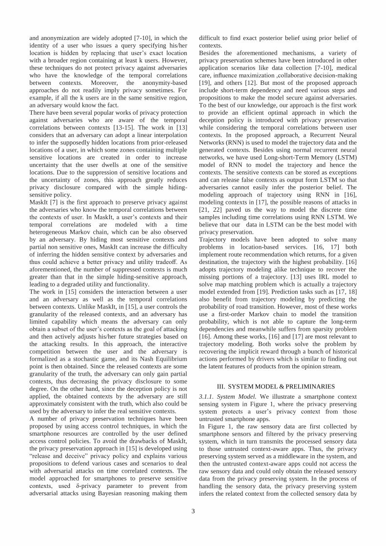
3
and anonymization are widely adopted [7-10], in which the
identity of a user who issues a query specifying his/her
location is hidden by replacing that user’s exact location
with a broader region containing at least k users. However,
these techniques do not protect privacy against adversaries
who have the knowledge of the temporal correlations
between contexts. Moreover, the anonymity-based
approaches do not readily imply privacy sometimes. For
example, if all the k users are in the same sensitive region,
an adversary would know the fact.
There have been several popular works of privacy protection
against adversaries who are aware of the temporal
correlations between contexts [13-15]. The work in [13]
considers that an adversary can adopt a linear interpolation
to infer the supposedly hidden locations from prior-released
locations of a user, in which some zones containing multiple
sensitive locations are created in order to increase
uncertainty that the user dwells at one of the sensitive
locations. Due to the suppression of sensitive locations and
the uncertainty of zones, this approach greatly reduces
privacy disclosure compared with the simple hiding-
sensitive policy.
MaskIt [7] is the first approach to preserve privacy against
the adversaries who know the temporal correlations between
the contexts of user. In MaskIt, a user’s contexts and their
temporal correlations are modeled with a time
heterogeneous Markov chain, which can be also observed
by an adversary. By hiding most sensitive contexts and
partial non sensitive ones, MaskIt can increase the difficulty
of inferring the hidden sensitive context by adversaries and
thus could achieve a better privacy and utility tradeoff. As
aforementioned, the number of suppressed contexts is much
greater than that in the simple hiding-sensitive approach,
leading to a degraded utility and functionality.
The work in [15] considers the interaction between a user
and an adversary as well as the temporal correlations
between contexts. Unlike MaskIt, in [15], a user controls the
granularity of the released contexts, and an adversary has
limited capability which means the adversary can only
obtain a subset of the user’s contexts as the goal of attacking
and then actively adjusts his/her future strategies based on
the attacking results. In this approach, the interactive
competition between the user and the adversary is
formalized as a stochastic game, and its Nash Equilibrium
point is then obtained. Since the released contexts are some
granularity of the truth, the adversary can only gain partial
contexts, thus decreasing the privacy disclosure to some
degree. On the other hand, since the deception policy is not
applied, the obtained contexts by the adversary are still
approximately consistent with the truth, which also could be
used by the adversary to infer the real sensitive contexts.
A number of privacy preservation techniques have been
proposed by using access control techniques, in which the
smartphone resources are controlled by the user defined
access control policies. To avoid the drawbacks of MaskIt,
the privacy preservation approach in [15] is developed using
“release and deceive” privacy policy and explains various
propositions to defend various cases and scenarios to deal
with adversarial attacks on time correlated contexts. The
model approached for smartphones to preserve sensitive
contexts, used δ-privacy parameter to prevent from
adversarial attacks using Bayesian reasoning making them
difficult to find exact posterior belief using prior belief of
contexts.
Besides the aforementioned mechanisms, a variety of
privacy preservation schemes have been introduced in other
application scenarios like data collection [7-10], medical
care, influence maximization ,collaborative decision-making
[19], and others [12]. But most of the proposed approach
include short-term dependency and need various steps and
propositions to make the model secure against adversaries.
To the best of our knowledge, our approach is the first work
to provide an efficient optimal approach in which the
deception policy is introduced with privacy preservation
while considering the temporal correlations between user
contexts. In the proposed approach, a Recurrent Neural
Networks (RNN) is used to model the trajectory data and the
generated contexts. Besides using normal recurrent neural
networks, we have used Long-short-Term Memory (LSTM)
model of RNN to model the trajectory and hence the
contexts. The sensitive contexts can be stored as exceptions
and can release false contexts as output form LSTM so that
adversaries cannot easily infer the posterior belief. The
modeling approach of trajectory using RNN in [16],
modeling contexts in [17], the possible reasons of attacks in
[21, 22] paved us the way to model the discrete time
samples including time correlations using RNN LSTM. We
believe that our data in LSTM can be the best model with
privacy preservation.
Trajectory models have been adopted to solve many
problems in location-based services. [16, 17] both
implement route recommendation which returns, for a given
destination, the trajectory with the highest probability. [16]
adopts trajectory modeling alike technique to recover the
missing portions of a trajectory. [13] uses IRL model to
solve map matching problem which is actually a trajectory
model extended from [19]. Prediction tasks such as [17, 18]
also benefit from trajectory modeling by predicting the
probability of road transition. However, most of these works
use a first-order Markov chain to model the transition
probability, which is not able to capture the long-term
dependencies and meanwhile suffers from sparsity problem
[16]. Among these works, [16] and [17] are most relevant to
trajectory modeling. Both works solve the problem by
recovering the implicit reward through a bunch of historical
actions performed by drivers which is similar to finding out
the latent features of products from the opinion stream.
III. SYSTEM MODEL & PRELIMINARIES
3.1.1. System Model. We illustrate a smartphone context
sensing system in Figure 1, where the privacy preserving
system protects a user’s privacy context from those
untrusted smartphone apps.
In Figure 1, the raw sensory data are first collected by
smartphone sensors and filtered by the privacy preserving
system, which in turn transmits the processed sensory data
to those untrusted context-aware apps. Thus, the privacy
preserving system served as a middleware in the system, and
then the untrusted context-aware apps could not access the
raw sensory data and could only obtain the released sensory
data from the privacy preserving system. In the process of
handling the sensory data, the privacy preserving system
infers the related context from the collected sensory data by
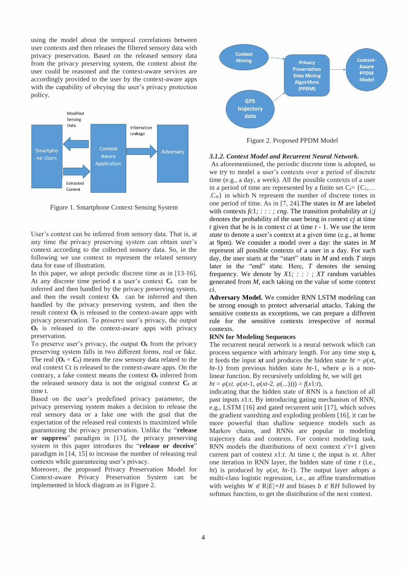
4
using the model about the temporal correlations between
user contexts and then releases the filtered sensory data with
privacy preservation. Based on the released sensory data
from the privacy preserving system, the context about the
user could be reasoned and the context-aware services are
accordingly provided to the user by the context-aware apps
with the capability of obeying the user’s privacy protection
policy.
Figure 1. Smartphone Context Sensing System
User’s context can be inferred from sensory data. That is, at
any time the privacy preserving system can obtain user’s
context according to the collected sensory data. So, in the
following we use context to represent the related sensory
data for ease of illustration.
In this paper, we adopt periodic discrete time as in [13-16].
At any discrete time period t a user’s context Ct can be
inferred and then handled by the privacy preserving system,
and then the result context Ot can be inferred and then
handled by the privacy preserving system, and then the
result context Ot is released to the context-aware apps with
privacy preservation. To preserve user’s privacy, the output
Ot is released to the context-aware apps with privacy
preservation.
To preserve user’s privacy, the output Ot from the privacy
preserving system falls in two different forms, real or fake.
The real (Ot = Ct) means the raw sensory data related to the
real context Ct is released to the context-aware apps. On the
contrary, a fake context means the context Ot inferred from
the released sensory data is not the original context Ct at
time t.
Based on the user’s predefined privacy parameter, the
privacy preserving system makes a decision to release the
real sensory data or a fake one with the goal that the
expectation of the released real contexts is maximized while
guaranteeing the privacy preservation. Unlike the “release
or suppress” paradigm in [13], the privacy preserving
system in this paper introduces the “release or deceive”
paradigm in [14, 15] to increase the number of releasing real
contexts while guaranteeing user’s privacy.
Moreover, the proposed Privacy Preservation Model for
Context-aware Privacy Preservation System can be
implemented in block diagram as in Figure 2.
Figure 2. Proposed PPDM Model
3.1.2. Context Model and Recurrent Neural Network.
As aforementioned, the periodic discrete time is adopted, so
we try to model a user’s contexts over a period of discrete
time (e.g., a day, a week). All the possible contexts of a user
in a period of time are represented by a finite set Ct= {C1,…
.CN} in which N represent the number of discrete times in
one period of time. As in [7, 24].The states in M are labeled
with contexts fc1; : : : ; cng. The transition probability at i;j
denotes the probability of the user being in context cj at time
t given that he is in context ci at time t - 1. We use the term
state to denote a user’s context at a given time (e.g., at home
at 9pm). We consider a model over a day: the states in M
represent all possible contexts of a user in a day. For each
day, the user starts at the “start” state in M and ends T steps
later in the “end” state. Here, T denotes the sensing
frequency. We denote by X1; : : : ; XT random variables
generated from M, each taking on the value of some context
ci.
Adversary Model. We consider RNN LSTM modeling can
be strong enough to protect adversarial attacks. Taking the
sensitive contexts as exceptions, we can prepare a different
rule for the sensitive contexts irrespective of normal
contexts.
RNN for Modeling Sequences
The recurrent neural network is a neural network which can
process sequence with arbitrary length. For any time step t,
it feeds the input xt and produces the hidden state ht = φ(xt,
ht-1) from previous hidden state ht-1, where φ is a non-
linear function. By recursively unfolding ht, we will get
ht = φ(xt, φ(xt-1, φ(xt-2, φ(...)))) = f(x1:t),
indicating that the hidden state of RNN is a function of all
past inputs x1:t. By introducing gating mechanism of RNN,
e.g., LSTM [16] and gated recurrent unit [17], which solves
the gradient vanishing and exploding problem [16], it can be
more powerful than shallow sequence models such as
Markov chains, and RNNs are popular in modeling
trajectory data and contexts. For context modeling task,
RNN models the distributions of next context x˜t+1 given
current part of context x1:t. At time t, the input is xt. After
one iteration in RNN layer, the hidden state of time t (i.e.,
ht) is produced by φ(xt, ht-1). The output layer adopts a
multi-class logistic regression, i.e., an affine transformation
with weights W ∈ R|E|×H and biases b ∈ RH followed by
softmax function, to get the distribution of the next context.

5
Mathematically,
p(˜ xt+1 = i|x1:t) =exp( j exp( WW[i,[j, :]:]hth+t +b[ib]) [j])
To adopt RNN in modeling trajectory, we can regard each
edge as a word/state and a trajectory as a sentence.
However, we want to highlight that the transition from one
word to any other word is free, while only the transitions
from one edge to its adjacent edges are possible. In other
words, the state transition of trajectory is strictly constrained
by the topology of road network. Nevertheless, we still can
hope RNN to be able to learn the topological constraints and
assign close-to zero probabilities to the transitions from one
edge ri to any edge rj that is not adjacent to ri. In the
following, we will prove that, in order for RNN to achieve
above objectives, the number of its hidden units has a lower
bound that depends on the state size |E|, the required error
and the l2-norm of the weights.
Problem Formulation
Our objective is to predict future locations and contexts of
users. Without loss of generality, we normalize the activity
information into the keyword representation.
Given the context keyword set C = { c(1); c(2); : : : ;
c(/C)},
User set U = { u(1); u(2); : : : ; u(/U/)}
and location set L = {l(1); l(2); : : : ; l(/L/)},
Thus, the check-in data required data can be defined as a
quadruple r = (u; l; c; t), indicating that user u visits
location l with context c at time t.
Here, for the ease of calculation, we discretize continuous
time t to hour of day and day of week. With these notations,
our problem can then be formulated as: Our goal is to
predict user u’s next location ln and preserve the sensitive
context c, given the next check-in time tn and the historical
check-in sequence.
Tn-1 = {r1, r2 …….. rn-1 }
Figure 3: Proposed RNN model
Figure 4. Context-aware Recurrent Unit
In Figure 3, Users denoted by Locations denoted by L,
Contexts denoted by C,Time denoted by T and S={0,1}
denote the sensitivity of contexts. Thus, the inputs to Linear
Unit of RNN can be a set of (U, l, C, t, S). If S=1, the input
is marked sensitive and thus released contexts must be
deceiving. As it is infeasible to take all 5 features as input
so, 2 inputs representing, sequential features and temporal
contexts are sent. Based on these features, we adopt gated
RNN as the shared hidden layer for modeling spatial-
activity topics. As we have discussed, it is infeasible to take
all five features together as the input of existing gated
RNNs. Thus we decompose input features into sequential
features xS n-1 (linear combination of u; an-1 and ln-1) and
temporal context xT n (linear combination of u; tn and sn).
Then we propose a novel Context Aware Recurrent Unit
(CARU) to integrate sequential feature xS n-1 and temporal
context xT n dynamically.
Context-Aware Recurrent Unit
The spatial-activity topics are influenced by not only the
sequential feature but also the temporal context. What’s
more, the sequential feature and temporal context cannot be
controlled by a single sigmoid gate. For example, when
sensitive contexts of user are applied the sigmoid function
must be different while the temporal context should play an
active role. Therefore, we propose the Context Aware
Recurrent Unit as in Figure 4. to integrate temporal and
sequential contexts dynamically.
Specifically, to capture the sequential pattern, we calculate
the sequential hidden state as follows:
where n denotes the time step, h is the hidden state of
CARU, hS is called as sequential hidden state, and i; f are
sigmoid gates. Here, W; U; V and b represent the weight
matrices and bias vectors, ∗ represents the element-wise
product of two vectors, σ(·) denotes the sigmoid function
and g(·) is the activation function (the hyperbolic tangent
function in our work). The calculation of the sequential
hidden state is similar to the
calculation of memory state of LSTM cell. Here, the major
difficulty in our problem is not the long-term dependency
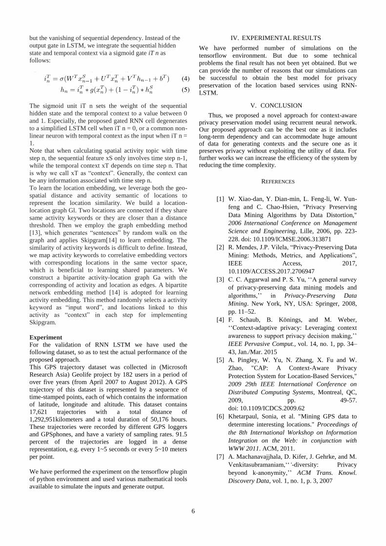
6
but the vanishing of sequential dependency. Instead of the
output gate in LSTM, we integrate the sequential hidden
state and temporal context via a sigmoid gate iT n as
follows:
The sigmoid unit iT n sets the weight of the sequential
hidden state and the temporal context to a value between 0
and 1. Especially, the proposed gated RNN cell degenerates
to a simplified LSTM cell when iT n = 0, or a common non-
linear neuron with temporal context as the input when iT n =
1.
Note that when calculating spatial activity topic with time
step n, the sequential feature xS only involves time step n-1,
while the temporal context xT depends on time step n. That
is why we call xT as “context”. Generally, the context can
be any information associated with time step n.
To learn the location embedding, we leverage both the geo-
spatial distance and activity semantic of locations to
represent the location similarity. We build a location-
location graph Gl. Two locations are connected if they share
same activity keywords or they are closer than a distance
threshold. Then we employ the graph embedding method
[13], which generates “sentences” by random walk on the
graph and applies Skipgram[14] to learn embedding. The
similarity of activity keywords is difficult to define. Instead,
we map activity keywords to correlative embedding vectors
with corresponding locations in the same vector space,
which is beneficial to learning shared parameters. We
construct a bipartite activity-location graph Ga with the
corresponding of activity and location as edges. A bipartite
network embedding method [14] is adopted for learning
activity embedding. This method randomly selects a activity
keyword as “input word”, and locations linked to this
activity as “context” in each step for implementing
Skipgram.
Experiment
For the validation of RNN LSTM we have used the
following dataset, so as to test the actual performance of the
proposed approach.
This GPS trajectory dataset was collected in (Microsoft
Research Asia) Geolife project by 182 users in a period of
over five years (from April 2007 to August 2012). A GPS
trajectory of this dataset is represented by a sequence of
time-stamped points, each of which contains the information
of latitude, longitude and altitude. This dataset contains
17,621 trajectories with a total distance of
1,292,951kilometers and a total duration of 50,176 hours.
These trajectories were recorded by different GPS loggers
and GPSphones, and have a variety of sampling rates. 91.5
percent of the trajectories are logged in a dense
representation, e.g. every 1~5 seconds or every 5~10 meters
per point.
We have performed the experiment on the tensorflow plugin
of python environment and used various mathematical tools
available to simulate the inputs and generate output.
IV. EXPERIMENTAL RESULTS
We have performed number of simulations on the
tensorflow environment. But due to some technical
problems the final result has not been yet obtained. But we
can provide the number of reasons that our simulations can
be successful to obtain the best model for privacy
preservation of the location based services using RNN-
LSTM.
V. CONCLUSION
Thus, we proposed a novel approach for context-aware privacy preservation model using recurrent neural network. Our proposed approach can be the best one as it includes long-term dependency and can accommodate huge amount of data for generating contexts and the secure one as it preserves privacy without exploiting the utility of data. For further works we can increase the efficiency of the system by reducing the time complexity.
REFERENCES
[1] W. Xiao-dan, Y. Dian-min, L. Feng-li, W. Yun-
feng and C. Chao-Hsien, "Privacy Preserving
Data Mining Algorithms by Data Distortion,"
2006 International Conference on Management
Science and Engineering, Lille, 2006, pp. 223-
228. doi: 10.1109/ICMSE.2006.313871
[2] R. Mendes, J.P. Vilela, “Privacy-Preserving Data
Mining: Methods, Metrics, and Applications”,
IEEE Access, 2017,
10.1109/ACCESS.2017.2706947
[3] C. C. Aggarwal and P. S. Yu, ‘‘A general survey
of privacy-preserving data mining models and
algorithms,’’ in Privacy-Preserving Data
Mining. New York, NY, USA: Springer, 2008,
pp. 11–52.
[4] F. Schaub, B. Könings, and M. Weber,
‘‘Context-adaptive privacy: Leveraging context
awareness to support privacy decision making,’’
IEEE Pervasive Comput., vol. 14, no. 1, pp. 34–
43, Jan./Mar. 2015
[5] A. Pingley, W. Yu, N. Zhang, X. Fu and W.
Zhao, "CAP: A Context-Aware Privacy
Protection System for Location-Based Services,"
2009 29th IEEE International Conference on
Distributed Computing Systems, Montreal, QC,
2009, pp. 49-57.
doi: 10.1109/ICDCS.2009.62
[6] Khetarpaul, Sonia, et al. "Mining GPS data to
determine interesting locations." Proceedings of
the 8th International Workshop on Information
Integration on the Web: in conjunction with
WWW 2011. ACM, 2011.
[7] A. Machanavajjhala, D. Kifer, J. Gehrke, and M.
Venkitasubramaniam,‘‘‘-diversity: Privacy
beyond k-anonymity,’’ ACM Trans. Knowl.
Discovery Data, vol. 1, no. 1, p. 3, 2007
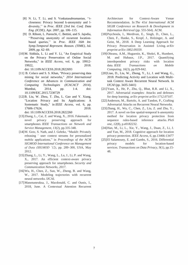
7
[8] N. Li, T. Li, and S. Venkatasubramanian, ‘‘t-
closeness: Privacy beyond k-anonymity and l-
diversity,’’ in Proc. IEEE 23rd Int. Conf. Data
Eng. (ICDE), Apr. 2007, pp. 106–115.
[9] D. Riboni, L. Pareschi, C. Bettini, and S. Jajodia,
‘‘Preserving anonymity of recurrent location-
based queries,’’ in Proc. IEEE 16th Int.
Symp.Temporal Represent. Reason. (TIME), Jul.
2009, pp. 62–69.
[10] M. Siddula, L. Li and Y. Li, "An Empirical Study
on the Privacy Preservation of Online Social
Networks," in IEEE Access, vol. 6, pp. 19912-
19922, 2018.
doi: 10.1109/ACCESS.2018.2822693
[11] B. Colaco and S. S. Khan, "Privacy preserving data
mining for social networks," 2014 International
Conference on Advances in Communication and
Computing Technologies (ICACACT 2014),
Mumbai, 2014, pp. 1-4. doi:
10.1109/EIC.2015.7230729
[12] B. Liu, W. Zhou, T. Zhu, L. Gao and Y. Xiang,
"Location Privacy and Its Applications: A
Systematic Study," in IEEE Access, vol. 6, pp.
17606-17624, 2018.
doi: 10.1109/ACCESS.2018.2822260
[13] Zhang, L., Cai, Z. and Wang, X., 2016. Fakemask: a
novel privacy preserving approach for
smartphones. IEEE Transactions on Network and
Service Management, 13(2), pp.335-348.
[14] M. Gotz, S. Nath, and J. Gehrke, “MaskIt: Privately
releasing ¨ user context streams for personalized
mobile applications,” in Proceedings of the ACM
SIGMOD International Conference on Management
of Data (SIGMOD ’12), pp. 289–300, USA, May
2012.
[15] Zhang, L., Li, Y., Wang, L., Lu, J., Li, P. and Wang,
X., 2017. An efficient context-aware privacy
preserving approach for smartphones. Security and
Communication Networks, 2017.
[16] Wu, H., Chen, Z., Sun, W., Zheng, B. and Wang,
W., 2017. Modeling trajectories with recurrent
neural networks. IJCAI.
[17] Manotumruksa, J., Macdonald, C. and Ounis, I.,
2018, June. A Contextual Attention Recurrent
Architecture for Context-Aware Venue
Recommendation. In The 41st International ACM
SIGIR Conference on Research & Development in
Information Retrieval (pp. 555-564). ACM.
[18] Psychoula, I., Merdivan, E., Singh, D., Chen, L.,
Chen, F., Hanke, S., Kropf, J., Holzinger, A. and
Geist, M., 2018. A Deep Learning Approach for
Privacy Preservation in Assisted Living. arXiv
preprint arXiv:1802.09359.
[19] Olteanu, A.M., Huguenin, K., Shokri, R., Humbert,
M. and Hubaux, J.P., 2017. Quantifying
interdependent privacy risks with location
data. IEEE Transactions on Mobile
Computing, 16(3), pp.829-842.
[20] Liao, D., Liu, W., Zhong, Y., Li, J. and Wang, G.,
2018. Predicting Activity and Location with Multi-
task Context Aware Recurrent Neural Network. In
IJCAI (pp. 3435-3441)
[21] Yuan, X., He, P., Zhu, Q., Bhat, R.R. and Li, X.,
2017. Adversarial examples: Attacks and defenses
for deep learning. arXiv preprint arXiv:1712.07107.
[22] Anderson, M., Bartolo, A. and Tandon, P., Crafting
Adversarial Attacks on Recurrent Neural Networks.
[23] Zhang, H., Wu, C., Chen, Z., Liu, Z. and Zhu, Y.,
2017. A novel on-line spatial-temporal k-anonymity
method for location privacy protection from
sequence rules-based inference attacks. PloS
one, 12(8), p.e0182232.
[24] Han, M., Li, L., Xie, Y., Wang, J., Duan, Z., Li, J.
and Yan, M., 2018. Cognitive approach for location
privacy protection. IEEE Access, 6, pp.13466-13477
[25] El Salamouny, E. and Gambs, S., 2016. Differential
privacy models for location-based
services. Transactions on Data Privacy, 9(1), pp.15-
48.

E-waste management in Nepal: An Approach for Minimizing E-waste to Ensure a Safe Environment.
Avhimanhu Sapkota.
BSc (Hons). Computing at The British College. 9860970274
ABSTRACT Electrical and electronic waste– e-waste – has become
a global environmental pollution problem in
developed and developing countries. Moreover,
management of these waste is a challenge for
developing countries like Nepal. The study covers the
effects of e-waste generation in the global scenario.
Meanwhile, current recycling practices, challenges
and the impact of e- waste in Nepal have been
comprehensively presented. On the basis of a
comparison between e- waste management in the
developed countries and Nepal, sustainable e- waste
management solutions have been proposed. The aim
of the research is to understand the importance of e-
waste management and to advise a sustainable e-
waste management system, which is used in developed
countries, to improve the quality of e- waste
management in Nepal.
(Keywords: E-waste, e-waste management, Nepal,
recycling practices, challenges, impact, comparison.)
1. INTRODUCTION Since new technology is constantly emerging from day
to day and more ICT equipment is produced, people
are looking forward to better ICT solutions. In the
meantime, people ignore the fact that electronic
devices contain toxic substances that cause a health
nightmare during its disposal and recycling. The
electronic products that have reached the end of their
lives are known as electronic waste or e-waste. The use
of electronic devices has increased dramatically in the
past decade and the number of devices disposed of is
growing extensively worldwide. E- waste
management is perhaps one of the fastest growing
pollution problems that can contaminate the
environment and pose a threat to human health.
In spite of the fact that e-waste management is a
problem for both developed and developing countries,
it is a major challenge for many developing countries
like Nepal, as e-waste is perhaps obscure to many
people in the country. Electronic gadgets which
contains toxic chemicals and heavy metals are
destroying Nepal’s beautiful ecosystem. In order to
minimize e- waste in Nepal and ensure a safe
environment, this problem must be addressed at both
the individual and the government levels.
2. LITERATURE REVIEW Electric and Electronic waste – e-waste – is electronic
devices that are almost at the end of its useful life. For
instance, old Cathode Ray Tube (CRT) computers,
outdated mobile phones, irreparable laptops and
tablets. “E-waste is an electrically powered appliance
that no longer satisfies the current owner for its
original purpose” (Sinha, 2004, p. 3). It contains
many different substances consisting of ferrous
metals, plastics, glass, concrete, rubber and toxic
substances such as barium, mercury, lead, cadmium
and flame retardants. The disposal and recycling of
these waste is a serious challenge for both developed
countries, because it pollutes the environment and
causes human beings to suffer frequently.
The world looks forward to e- waste management, but
the rate of e- waste generated is far higher than the rate
of e- waste recycled. In 2014, around 42.8 million tons
of electrical waste were generated worldwide, but only
15- 20 percent of all electrical waste was recycled
(Leblanc, 2018). Today, about 40.7 percent of the
world 's e- waste is generated in Asia, 27.5 percent in
Europe and 25.3 percent in the Americas (Balde et. al.,
2017). Many countries including Denmark, Austria,
Germany, Australia and the Netherlands have begun
to recognize the importance of e- waste, and have
bandaged e- waste into landfills. In addition, the rate
of e- waste recycled is increasing gradually. Many
countries have built e- waste recycling companies that
provide more than 296 jobs per year for every 10,000

tons of recycled e- waste (Leblanc, 2018). E- waste
management therefore ensures a safe environment,
saves energy and makes a significant contribution to
the economy of a particular region.
3. E-WASTE IN NEPAL In Nepal, the rate of imports of electronic devices has
been accelerating every day, while the disposal of
electronic waste is challenging because it has a
negative recycling practices and contains harmful
materials. The large portion of the e- waste in Nepal
consists of old CRT monitors, washing machines,
refrigerators and inverter batteries. According to a
study by the Environment Department of Nepal,
Kathmandu discarded 18,000 metric tons of e- waste
in 2017 (Awale, 2018). Nepal does not have a culture
of repair, reuse and recycle, as there are no specific
centers for recycling e-wastes.
Moreover, people here are not aware of the impact of
e- waste and the importance of e- waste management.
In Nepal, according to the survey, only 35 percent of
people were aware of e- waste and its harmful effects
(Karmacharya et al., 2017). As a consequence, the
majority of the old and irreparable electronic goods are
disposed of as garbage or sold to scrap dealers.
In addition, Nepal has no separate legislation
specifically for e- waste, which allows these scrap
dealers to take advantage of it and unsafely dismantle
the useful metals then dump the hazardous wastes
into landfills.
4. E-WASTE MANAGEMENT
SYSTEMS IN DEVELOPED
COUNTRIES.
4.1 Public awareness.
The awareness of electronic waste and its
environmental and human health impacts must be the
first step in the proper management of electronic
waste. If many people know the importance of e- waste
management, they will become aware of it and
encourage the government to manage e- waste and
support the individual level as well. In Germany, the
government began awareness education using
unemployed people to raise public awareness on
health and environmental impacts of e- waste (Adeola
and Othman, 2011).
4.2 Recycling.
Recycling is the key to reducing electronic waste, as it
has environmental benefits at every stage of the
electronics production life cycle. Many developed
countries have perhaps used various methodologies to
recycle e-waste. In Japan, electronic devices that fall
under home appliances must be recovered and
recycled by manufacturers in order to use resources
effectively (Adeola and Othman, 2011).
4.3 Legislations and Policies.
The law of the county binds people and makes them
aware of their duties. Systematic management of e-
waste will perhaps be effective through strict laws and
policies. The government should enforce strict laws
against illegal disposal of e-waste. For example, India
has now banded e- waste imports from other countries
and enforced a law to prevent e- waste landfills.
5. E-WASTE MANAGEMENT IN
NEPAL. As a developing country, Nepal has shipped most of
its electronic waste to India, where it is leached
chemically to extract valuable elements. However,
Nepal will now have to build processing plants,
following the bandage of e-waste imports in India.
As stated above, e- waste management ensures a safe
environment if e- waste is managed or recycled
properly. In the meantime, this is an opportunity to
reduce the unemployment problem in Nepal. The
establishment of recycling centers and waste
collectors provides many unemployed people, in
Nepal, with job opportunities. In addition, precious
elements such as gold and silver extracted from e-
waste can generate a good amount of money that will
perhaps contribute to the national economy. The
establishment of e-waste management system is like
killing two birds with one stone.
6. PROPOSED E-WASTE
MANAGEMENT SOLUTIONS. In comparison with e- waste management systems in
developed countries, some of the e- waste
management system applicable to Nepal has been
discussed below:
6.1 Awareness through ICT.
It was quite clear that most people in Nepal are not
aware of the impact of e- waste and the importance of
e- waste management. Since most people who use
electronic goods are responsible for generating
electronic waste, awareness with the help of ICT is

more convenient. For example, the government and
other organizations in Nepal can advertise and share
awareness through all social media, TV and other ICT
devices that support video or audio streaming. In
addition, awareness campaigns could be carried out to
encourage people, in rural and urban areas, to dispose
e-waste separately.
6.2 Establishment of recycling plants.
The establishment of recycling plants or centers is the
most significant step in solutions for e- waste
management, because recycling is the best way to deal
with e- wastes. Recycling centers must collect and
recycle e-waste generated in various parts of the
country appropriately. First, they have to manually
dismantle e- wastes. They must then either recycle the
waste using the chemicals and biological leaching
process or import recycling machines. However,
biological and chemical leaching in Nepal would be
cost- effective because recycling machines are
expensive.
6.3 E-waste Policies and Legislations.
The Nepalese government must study the future of e-
waste and the impact that e- waste can have on people
and the environment. They must therefore enforce
strict rules and regulations that oblige people to be
concerned about the generated e- waste. For instance,
the government must enforce laws which encourages
people to repair, reuse and recycle electronic waste. In
addition, they must also make people return e- waste
to retailers instead of disposing of it to municipal
waste, who must then give it to recycling centers.
Strict punishments should also be imposed on people
who have improperly disposed electronic waste.
7. CONCLUSION In conclusion, e- waste is a serious problem both at
local and global level. Many developed countries,
however, manage their e- wastes properly, but
developing countries face it as a challenge. Most of the
people in Nepal do not know about e-waste and its
management. The government also seems to be
unaware of the fact that laws relating to e-waste have
not yet been enforced. Lastly, no recycling centers
have been established to recycle e-waste
appropriately. E-waste in Nepal are therefore treated
as solid wastes and dumped into landfills. Despite the
fact that Nepal can be the victim of e- waste impacts,
it is necessary to manage these waste as soon as
possible.
Efforts and research on e- waste recycling are being
carried out in different parts of the world in a
sustainable manner. Strict laws and regulations may be
included in future efforts to overcome e- waste
management problems. Moreover, they may also
include chemical and biological leaching
methodologies for recycling e-waste. Some solutions
have been proposed, including recycling plants, strict
policies and awareness, to overcome Nepal's
unmanaged e- waste. Therefore, the world should be
aware of the impacts of e- waste and how it can be
disposed of and find a sustainable method of e- waste
management to ensure a safe environment and a
healthy human life.
REFERENCES
Adeola, A. M. and Othman M. (2011) An overview
of ICT waste management: Suggestions of best
practices from developed countries to developing
nations (Nigeria), Proceedings of the 7th
International Conference on Networked
Computing, pp. 109-115.
Awale, S. (2018) What will Nepal do with its e-waste?
Nepali Times, 925 August-September, pp. 8-9.
Balde, C. P. Forti, V. Kuehr, R. and Stegmann, P.
(2017) Regional E-waste Status and Trends. In: The
Global E-waste Monitor 2017: Quantities, Flows,
and Resources. Bonn/Geneva/Vienna: United
Nations University (UNU), International
Telecommunication Union (ITU) & International
Solid Waste Association (ISWA) pp. 64-73.
Karmacharya, A. Basnet, P. and Rana, V. K. (2017)
Status of e-Waste in Nepal and its Mitigating
Measures through Information Communication
Technology. Proceedings of the National Students’
Conference on Information Technology, p.2.
Leblanc, R. (2018) E-Waste Recycling Facts and
Figures [Online]. Available from:
<https://www.thebalancesmb.com> [Accessed 13th
December 2018].
Sinha, D. (2004) The Management of Electronic
Waste: A Comparative Study on India and
Switzerland [Master Thesis]. University of St. Gallen.

1
Abstract—Software Defined Network (SDN) is a new network architecture for designing, building, and managing networks that
separates the network’s control plane and forwarding plane to better support the scalability and innovation in a network
infrastructure. The overall network performance of an application is mostly affected by the two major factors, bandwidth, and
latency. Between each pair of network elements in network infrastructure, there may exist multiple paths connecting them with
different properties. A traditional network does not take this knowledge into Consideration and may result in sub-optimal
performance of applications and underutilization of a network resource. This research proposes a concept of Application aware
routing which could improve the overall performance of a network by categorizing the application in bandwidth oriented and
latency oriented and allocate the separate route for each type of traffic based on the application preferences using Software
defined network architecture and OpenFlow protocol. The research also proposes a design of an application aware network
topology by using software defined network architecture which uses open flow protocol and open flow protocol based controller.
Routes for the application packets are chosen based on the application type. To verify the feasibility and practical implementation
of the proposed concept SDN topology is implemented in emulated environment using mininet)
Keywords— Software defined network, OpenFlow, application aware routing, Latency and bandwidth aware network.
I. INTRODUCTION1
In the today’s modern world, networking is inevitable which
plays a very important role in our society and has a
tremendous impact on humankind. As a foundation of an
information network, a reliable and highly efficient
networking infrastructure is a requirement of today’s world
of cloud computing and big data. With increasing
requirement of users and high resource demands of modern
applications, it is becoming increasingly difficult for the
traditional networking architecture, designed many years
ago, to satisfy the current requirements. In traditional
network architecture, network functionality is implemented
in a dedicated hardware in ASCI chips, which makes nearly
impossible to enhance features and fix bugs for the
customers on their own. Traditional configuration is time-
consuming and error-prone as IT administrator needs to
perform many steps to add or remove a single device from
network infrastructure [1]. Traditional network
infrastructure is a composed of multi-vendor devices as
multi-vendor environments require a high level of expertise
to complete a configuration, an administrator will therefore
need extensive knowledge of all present devices types [2].
The problem also exists in network routing mechanism as
most of the routing protocols calculate a single best route,
which will ultimately use by all application, which may not
be suited for all applications. The purpose of this research is
to design a software-defined network based network
architecture, which solves applications diverse requirements
with different properties to route application packets as per
application preferences to enhance the overall utilization of
the network resources. SDN is a computer network
architecture in which the control plane (routing) is
decoupled from the data plane (packet switching) in order to
make network and service management simpler, cheaper
and more flexible. SDN is dynamic, manageable, cost-
effective, and adaptable, making it ideal for high-
bandwidth, dynamic nature of today’s applications, SDN
based architecture gives more information about the state of
the entire network from the controller to applications [3].
This is in contrast to traditional distributed network
Architecture where intelligence and switching functions
coexist within the same physical device, resulting in
complex and ”ossified” networks. In SDN Control plane
and data plane interaction is done through a communication
protocol that is an open vendor-independent API. Open
Flow is the first and most dominant standard
communication interface for SDN. There are other
alternatives of Open Flow like Yang and NetConf.
Currently SDN is used for custom routing and service
Application aware route optimization in SDN
using bandwidth and latency
Manoj Gautam Kumar pudashine
Department of Computer Science and Engineering Department of Computer science and Engineering
Nepal College of Information Technology Nepal College of Information Technology
Pokhara University Pokhara University
Kathmandu Nepal Kathmandu Nepal
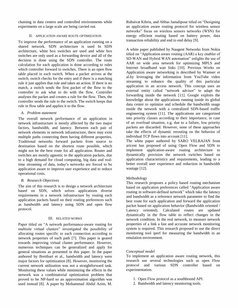
chaining in data centers and controlled environments while
experiments on a large scale are being carried out.
II. APPLICATION AWARE ROUTE OPTIMIZATION
To improve the performance of an application running on a
shared network. SDN architecture is used In SDN
architecture, white box switches are used and white box
switches are only used as a forwarding device and all of the
decision is done using the SDN controller. The route
calculation for each application is done according to rules
which controller forward to switches. There is an open flow
table placed in each switch. When a packet arrives at the
switch, switch checks for the entry and if there is a matching
rule it just applies that rule and takes an action. If there is no
match, a switch sends the first packet of the flow to the
controller to ask what to do with the flow. Controller
analyses the packet and creates a rule for the flow. Then, the
controller sends the rule to the switch. The switch keeps that
rule in flow table and applies it to the flow.
A. Problem statement
The overall network performance of an application in
network infrastructure is mostly affected by the two major
factors, bandwidth, and latency. Between each pair of
network elements in network infrastructure, there may exist
multiple paths connecting them having different properties.
Traditional networks forward packets from source to
destination based on the shortest route possible, which
might not be the best route for all application. Router and
switches are mostly agnostic to the application packets, due
to a high demand for cloud computing, big data and real-
time streaming of data, today’s networks are forced to be
application aware to improve user experience and to reduce
operational costs.
B. Research Objectives
The aim of this research is to design a network architecture
based on SDN, which solves applications diverse
requirements in a network infrastructure by routing each
application packets based on their routing preferences such
as bandwidth and latency using SDN and open flow
protocol.
III. RELATED WORKS
Paper titled on “A network performance-aware routing for
multisite virtual clusters” investigated the possibility of
allocating routes specific to each connection according to
network properties of each path [7]. This paper is geared
towards improving virtual cluster performance. However,
numerous techniques can be generalized and apply for
general situations as presented in this paper. In the paper
authored by Breitbart et al., bandwidth and latency were
major factors for optimization [8]. However, monitoring the
current network utilization was not a straightforward task.
Monitoring these values while minimizing the effects in the
network was a combinatorial optimization problem that
proved to be NP-hard so an approximation algorithm was
used instead [8]. A paper by Mohammad Abdul Azim, M.
Rubaivat Kibria, and Abbas Jamalipour titled on “Designing
an application aware routing protocol for wireless sensor
networks” focus on wireless sensors networks (WSN) for
energy efficient routing based on battery power, data
transaction reliability and end to end delay [9].
A white paper published by Naugent Networks from Nokia
titled on “Application aware routing (AAR) a key enabler of
SD-WAN and Hybrid WAN automation” enlights the use of
AAR on wide area network for optimizing MPLS and
Internet broadband wan links [10]. Previous Works on
Application aware networking is described by Wamser et
al.by leveraging the information from YouTube video
streaming to enhance the quality of this particular
application in an access network. This concept uses an
external entity called “network advisor” to adapt the
forwarding inside the network [11]. Google exploits the
knowledge about the applications running inside its global
data center to optimize and schedule the bandwidth usage
inside the network with a centralized SDN-based traffic
engineering system [11]. The applications are categorized
into priority classes according to their importance, in case
of an overload situation, e.g. due to a failure, low priority
packets are discarded. However, none of these approaches
take the effects of dynamic rerouting on the behavior of
individual TCP flows into account [11].
The white paper authored by SARO VELRAJAN from
aricent has proposed of using Open Flow and SDN to
implement application-aware routing architecture to
dynamically provision the network switches based on
application characteristics and requirements, leading to a
better overall user experience and reduction in bandwidth
wastage [12].
Methodology
This research proposes a policy based routing mechanism
based on application preferences called "Application aware
routing in software-defined network” which take the latency
and bandwidth as a reference network parameter to find the
best route for each application and forward the application
packet based on application behavior (Bandwidth oriented /
Latency oriented). Calculated routes are updated
dynamically in the flow table to reflect changes in the
network condition. In the real network, to measure network
properties of a link a fast and accurate network monitoring
system is required. This research proposed to use the direct
monitoring tool iperf for measuring the bandwidth in an
emulation environment.
Conceptual model
To implement an application aware routing network, this
research use several technologies such as open Flow
protocol and various SDN controller based on
experimentation.
1. Open Flow protocol as a southbound API.
2. Bandwidth and latency monitoring tools.
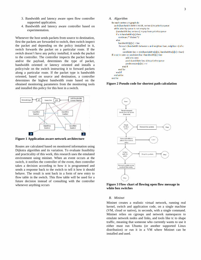
3
3. Bandwidth and latency aware open flow controller
supported application.
4. Bandwidth and latency aware controller based on
experimentation.
Whenever the host sends packets from source to destination,
first the packets are forwarded to switch, then switch inspect
the packet and depending on the policy installed in it,
switch forwards the packet on a particular route. If the
switch doesn’t have any policy installed, it sends the packet
to the controller. The controller inspects the packet header
and/or the payload, determines the type of packet,
bandwidth oriented or latency oriented and installs a
policy/rule on the switch instructing it to forward packets
along a particular route. If the packet type is bandwidth
oriented, based on source and destination, a controller
determines the highest bandwidth route based on the
obtained monitoring parameters from the monitoring tools
and installed this policy for this host in a switch.
Figure 1 Application aware network architecture
Routes are calculated based on monitored information using
Dijkstra algorithm and its variation. To evaluate feasibility
and practicality of this work, this research uses the emulated
environment using mininet. When an event occurs at the
switch, it notifies the controller of the event, then controller
takes a decision according to how it is programmed and
sends a response back to the switch to tell it how it should
behave. The result is sent back in a form of new entry to
flow table in the switch. This flow table will be used for a
future decision instead of consulting with the controller
whenever anything occurs
A. Algorithm
Figure 2 Pseudo code for shortest path calculation
Figure 3 Flow chart of flowing open flow message in
white box switches
B. Mininet
Mininet creates a realistic virtual network, running real
kernel, switch and application code, on a single machine
(VM, cloud or native), in seconds, with a single command.
Mininet relies on cgroups and network namespaces to
emulate network nodes and links, and tools like tc to shape
traffic, meaning that someone who currently wants to use it
either must run Ubuntu (or another supported Linux
distribution) or run it in a VM where Mininet can be
installed and used.
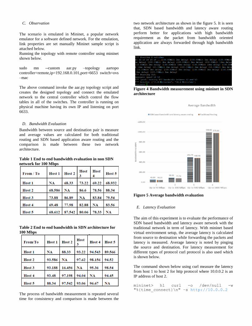
C. Observation
The scenario is emulated in Mininet, a popular network
emulator for a software defined network. For the emulation,
link properties are set manually Mininet sample script is
attached below.
Running the topology with remote controller using mininet
shown below.
sudo mn --custom aar.py –topology aartopo
controller=remote,ip=192.168.0.101,port=6653 switch=ovs
–mac
The above command invoke the aar.py topology script and
creates the designed topology and connect the emulated
network to the central controller which control the flow
tables in all of the switches. The controller is running on
physical machine having its own IP and listening on port
6633.
D. Bandwidth Evaluation
Bandwidth between source and destination pair is measure
and average values are calculated for both traditional
routing and SDN based application aware routing and the
comparison is made between these two network
architecture.
Table 1 End to end bandwidth evaluation in non SDN
network for 100 Mbps
Table 2 End to end bandwidth in SDN architecture for
100 Mbps
The process of bandwidth measurement is repeated several
time for consistency and comparison is made between the
two network architecture as shown in the figure 5. It is seen
that, SDN based bandwidth and latency aware routing
perform better for applications with high bandwidth
requirement as the packet from bandwidth oriented
application are always forwarded through high bandwidth
link.
Figure 4 Bandwidth measurement using mininet in SDN
architecture
Figure 5 Average bandwidth evaluation
E. Latency Evaluation
The aim of this experiment is to evaluate the performance of
SDN based bandwidth and latency aware network with the
traditional network in term of latency. With mininet based
virtual environment setup, the average latency is calculated
from source to destination while forwarding the packets and
latency is measured. Average latency is noted by pinging
the source and destination. For latency measurement for
different types of protocol curl protocol is also used which
is shown below.
The command shown below using curl measure the latency
from host 1 to host 2 for http protocol where 10.0.0.2 is an
IP address of host 2.
mininet> h1 curl -o /dev/null -w
"%{time_connect}\n" –s http://10.0.0.2
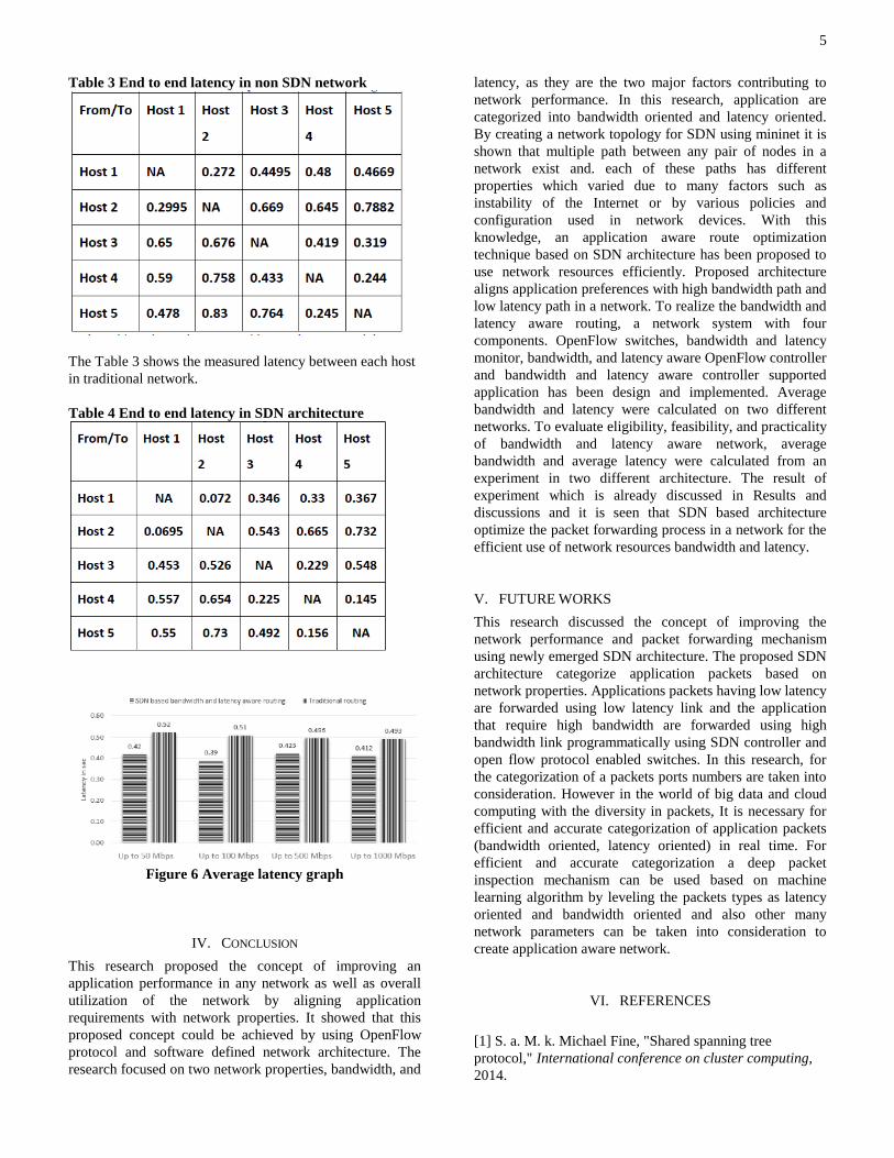
5
Table 3 End to end latency in non SDN network
The Table 3 shows the measured latency between each host
in traditional network.
Table 4 End to end latency in SDN architecture
Figure 6 Average latency graph
IV. CONCLUSION
This research proposed the concept of improving an
application performance in any network as well as overall
utilization of the network by aligning application
requirements with network properties. It showed that this
proposed concept could be achieved by using OpenFlow
protocol and software defined network architecture. The
research focused on two network properties, bandwidth, and
latency, as they are the two major factors contributing to
network performance. In this research, application are
categorized into bandwidth oriented and latency oriented.
By creating a network topology for SDN using mininet it is
shown that multiple path between any pair of nodes in a
network exist and. each of these paths has different
properties which varied due to many factors such as
instability of the Internet or by various policies and
configuration used in network devices. With this
knowledge, an application aware route optimization
technique based on SDN architecture has been proposed to
use network resources efficiently. Proposed architecture
aligns application preferences with high bandwidth path and
low latency path in a network. To realize the bandwidth and
latency aware routing, a network system with four
components. OpenFlow switches, bandwidth and latency
monitor, bandwidth, and latency aware OpenFlow controller
and bandwidth and latency aware controller supported
application has been design and implemented. Average
bandwidth and latency were calculated on two different
networks. To evaluate eligibility, feasibility, and practicality
of bandwidth and latency aware network, average
bandwidth and average latency were calculated from an
experiment in two different architecture. The result of
experiment which is already discussed in Results and
discussions and it is seen that SDN based architecture
optimize the packet forwarding process in a network for the
efficient use of network resources bandwidth and latency.
V. FUTURE WORKS
This research discussed the concept of improving the
network performance and packet forwarding mechanism
using newly emerged SDN architecture. The proposed SDN
architecture categorize application packets based on
network properties. Applications packets having low latency
are forwarded using low latency link and the application
that require high bandwidth are forwarded using high
bandwidth link programmatically using SDN controller and
open flow protocol enabled switches. In this research, for
the categorization of a packets ports numbers are taken into
consideration. However in the world of big data and cloud
computing with the diversity in packets, It is necessary for
efficient and accurate categorization of application packets
(bandwidth oriented, latency oriented) in real time. For
efficient and accurate categorization a deep packet
inspection mechanism can be used based on machine
learning algorithm by leveling the packets types as latency
oriented and bandwidth oriented and also other many
network parameters can be taken into consideration to
create application aware network.
VI. REFERENCES
[1] S. a. M. k. Michael Fine, "Shared spanning tree
protocol," International conference on cluster computing,
2014.

[2] O. N. Foundation, "OpenFlow Switch Specification,"
Open Networking Foundation, 2012.
[3] E. Y. K. Er. Jaspreet Singh, "Network Management
using Software Defined Networking," International Journal
of Advanced Research in Computer Science, vol. 8, p. 5,
2017.
[4] K. I. H. Abe., "A network performance-aware routing
for multisite virtual clusters," IEEE International
Conference on Networks (ICON), pp. 1-5, 2013.
[5] C.-Y. C. C.-Y. C. M. G. R. R. Y. Breitbart, "Efficiently
monitoring bandwidth and latency in IP networks.,"
Conference on Computer Communications Twentieth
Annual Joint Conference of the IEEE Computer and
Communications Society, vol. 2, pp. 933-942, 2001.
[6] M. M. Jamalipour, "Designing an application aware
routing protocol for wireless sensors networks," IEEE
GlobeCom, 2008.
[7] M. M. Gary Kinghorn, "Nuage Networks," Nuage
Networks, 21 12 2016. [Online]. Available:
http://www.nuagenetworks.net/blog/aar/. [Accessed 02
March 2018].
[8] M. J. A. B. F. W. W. K. Thomas Zinner, "Dynamic
Application-Aware Resource Management Using Software-
Defined Networking: Implementation Prospects and
Challenges," IEEE, pp. 1-6, 2014.
[9] Velrajan, "Application Aware Routing in Software
Defined Networks," Aricent Networks, 2013.
[10] Mininet, "Mininet," Mininet , March 2016. [Online].
Available:
https://github.com/mininet/mininet/wiki/Introduction-to-
Mininet. [Accessed January 2017].
[11] A. E. F. A. E. E. Kamal Benzekki, "Software-defined
networking (SDN): a survey," Laboratory of Computer
Networks and Systems Ismail University, 2017.
[12] K. I. P. U. D. H. A. Pongsakorn U-chupala, "Designing
of SDN-Assisted Bandwidth and Latency Aware," IPSJ
SIG, 2015.
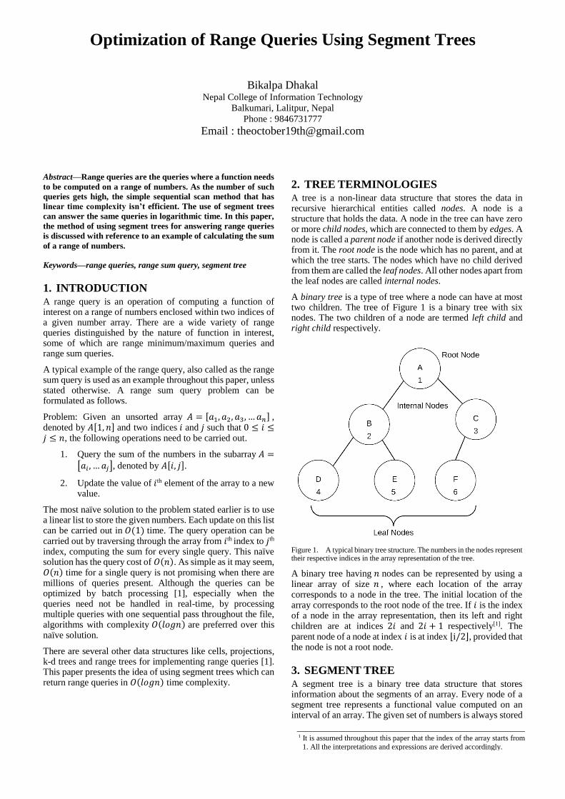
Optimization of Range Queries Using Segment Trees
Bikalpa Dhakal Nepal College of Information Technology
Balkumari, Lalitpur, Nepal
Phone : 9846731777
Email : [email protected]
Abstract—Range queries are the queries where a function needs
to be computed on a range of numbers. As the number of such
queries gets high, the simple sequential scan method that has
linear time complexity isn’t efficient. The use of segment trees
can answer the same queries in logarithmic time. In this paper,
the method of using segment trees for answering range queries
is discussed with reference to an example of calculating the sum
of a range of numbers.
Keywords—range queries, range sum query, segment tree
1. INTRODUCTION
A range query is an operation of computing a function of interest on a range of numbers enclosed within two indices of a given number array. There are a wide variety of range queries distinguished by the nature of function in interest, some of which are range minimum/maximum queries and range sum queries.
A typical example of the range query, also called as the range sum query is used as an example throughout this paper, unless stated otherwise. A range sum query problem can be formulated as follows.
Problem: Given an unsorted array 𝐴 = [𝑎1, 𝑎2, 𝑎3, … 𝑎𝑛] , denoted by 𝐴[1, 𝑛] and two indices 𝑖 and 𝑗 such that 0 ≤ 𝑖 ≤𝑗 ≤ 𝑛, the following operations need to be carried out.
1. Query the sum of the numbers in the subarray 𝐴 =[𝑎𝑖 , … 𝑎𝑗], denoted by 𝐴[𝑖, 𝑗].
2. Update the value of 𝑖th element of the array to a new value.
The most naïve solution to the problem stated earlier is to use a linear list to store the given numbers. Each update on this list can be carried out in 𝑂(1) time. The query operation can be carried out by traversing through the array from 𝑖th index to 𝑗th index, computing the sum for every single query. This naïve solution has the query cost of 𝑂(𝑛). As simple as it may seem, 𝑂(𝑛) time for a single query is not promising when there are millions of queries present. Although the queries can be optimized by batch processing [1], especially when the queries need not be handled in real-time, by processing multiple queries with one sequential pass throughout the file, algorithms with complexity 𝑂(𝑙𝑜𝑔𝑛) are preferred over this naïve solution.
There are several other data structures like cells, projections, k-d trees and range trees for implementing range queries [1]. This paper presents the idea of using segment trees which can return range queries in 𝑂(𝑙𝑜𝑔𝑛) time complexity.
2. TREE TERMINOLOGIES
A tree is a non-linear data structure that stores the data in recursive hierarchical entities called nodes. A node is a structure that holds the data. A node in the tree can have zero or more child nodes, which are connected to them by edges. A node is called a parent node if another node is derived directly from it. The root node is the node which has no parent, and at which the tree starts. The nodes which have no child derived from them are called the leaf nodes. All other nodes apart from the leaf nodes are called internal nodes.
A binary tree is a type of tree where a node can have at most two children. The tree of Figure 1 is a binary tree with six nodes. The two children of a node are termed left child and right child respectively.
Figure 1. A typical binary tree structure. The numbers in the nodes represent their respective indices in the array representation of the tree.
A binary tree having 𝑛 nodes can be represented by using a linear array of size 𝑛 , where each location of the array corresponds to a node in the tree. The initial location of the array corresponds to the root node of the tree. If 𝑖 is the index of a node in the array representation, then its left and right children are at indices 2𝑖 and 2𝑖 + 1 respectively[1]. The parent node of a node at index 𝑖 is at index ⌊i/2⌋, provided that the node is not a root node.
3. SEGMENT TREE
A segment tree is a binary tree data structure that stores information about the segments of an array. Every node of a segment tree represents a functional value computed on an interval of an array. The given set of numbers is always stored
1 It is assumed throughout this paper that the index of the array starts from
1. All the interpretations and expressions are derived accordingly.
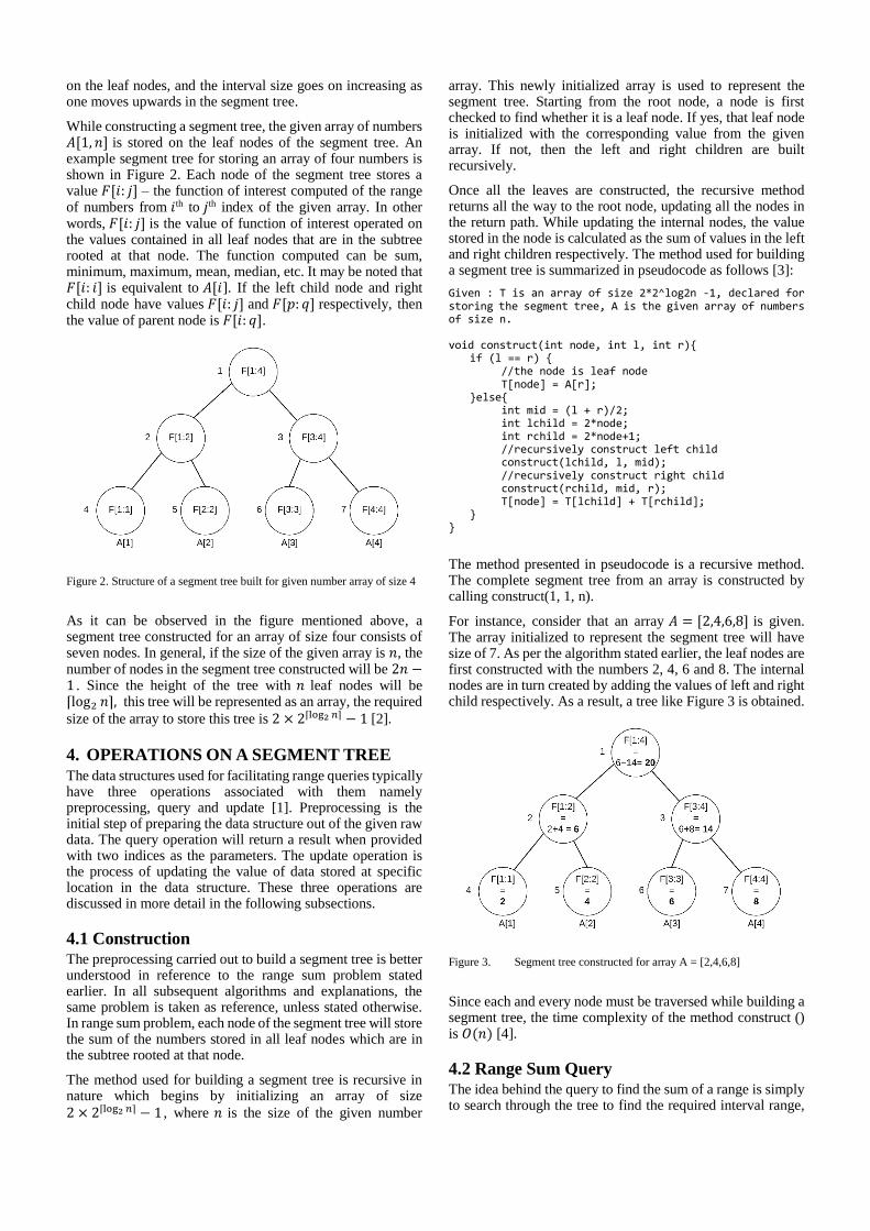
on the leaf nodes, and the interval size goes on increasing as one moves upwards in the segment tree.
While constructing a segment tree, the given array of numbers 𝐴[1, 𝑛] is stored on the leaf nodes of the segment tree. An example segment tree for storing an array of four numbers is shown in Figure 2. Each node of the segment tree stores a value 𝐹[𝑖: 𝑗] – the function of interest computed of the range of numbers from 𝑖th to 𝑗th index of the given array. In other words, 𝐹[𝑖: 𝑗] is the value of function of interest operated on the values contained in all leaf nodes that are in the subtree rooted at that node. The function computed can be sum, minimum, maximum, mean, median, etc. It may be noted that 𝐹[𝑖: 𝑖] is equivalent to 𝐴[𝑖]. If the left child node and right child node have values 𝐹[𝑖: 𝑗] and 𝐹[𝑝: 𝑞] respectively, then the value of parent node is 𝐹[𝑖: 𝑞].
Figure 2. Structure of a segment tree built for given number array of size 4
As it can be observed in the figure mentioned above, a segment tree constructed for an array of size four consists of seven nodes. In general, if the size of the given array is 𝑛, the number of nodes in the segment tree constructed will be 2𝑛 −1 . Since the height of the tree with 𝑛 leaf nodes will be ⌈log2 𝑛⌉, this tree will be represented as an array, the required
size of the array to store this tree is 2 × 2⌈log2 𝑛⌉ − 1 [2].
4. OPERATIONS ON A SEGMENT TREE
The data structures used for facilitating range queries typically have three operations associated with them namely preprocessing, query and update [1]. Preprocessing is the initial step of preparing the data structure out of the given raw data. The query operation will return a result when provided with two indices as the parameters. The update operation is the process of updating the value of data stored at specific location in the data structure. These three operations are discussed in more detail in the following subsections.
4.1 Construction The preprocessing carried out to build a segment tree is better understood in reference to the range sum problem stated earlier. In all subsequent algorithms and explanations, the same problem is taken as reference, unless stated otherwise. In range sum problem, each node of the segment tree will store the sum of the numbers stored in all leaf nodes which are in the subtree rooted at that node.
The method used for building a segment tree is recursive in nature which begins by initializing an array of size
2 × 2⌈log2 𝑛⌉ − 1 , where 𝑛 is the size of the given number
array. This newly initialized array is used to represent the segment tree. Starting from the root node, a node is first checked to find whether it is a leaf node. If yes, that leaf node is initialized with the corresponding value from the given array. If not, then the left and right children are built recursively.
Once all the leaves are constructed, the recursive method returns all the way to the root node, updating all the nodes in the return path. While updating the internal nodes, the value stored in the node is calculated as the sum of values in the left and right children respectively. The method used for building a segment tree is summarized in pseudocode as follows [3]:
Given : T is an array of size 2*2^log2n -1, declared for storing the segment tree, A is the given array of numbers of size n. void construct(int node, int l, int r){ if (l == r) { //the node is leaf node T[node] = A[r]; }else{ int mid = (l + r)/2; int lchild = 2*node; int rchild = 2*node+1; //recursively construct left child construct(lchild, l, mid); //recursively construct right child construct(rchild, mid, r); T[node] = T[lchild] + T[rchild]; } }
The method presented in pseudocode is a recursive method. The complete segment tree from an array is constructed by calling construct(1, 1, n).
For instance, consider that an array 𝐴 = [2,4,6,8] is given. The array initialized to represent the segment tree will have size of 7. As per the algorithm stated earlier, the leaf nodes are first constructed with the numbers 2, 4, 6 and 8. The internal nodes are in turn created by adding the values of left and right child respectively. As a result, a tree like Figure 3 is obtained.
Figure 3. Segment tree constructed for array A = [2,4,6,8]
Since each and every node must be traversed while building a segment tree, the time complexity of the method construct () is 𝑂(𝑛) [4].
4.2 Range Sum Query The idea behind the query to find the sum of a range is simply to search through the tree to find the required interval range,
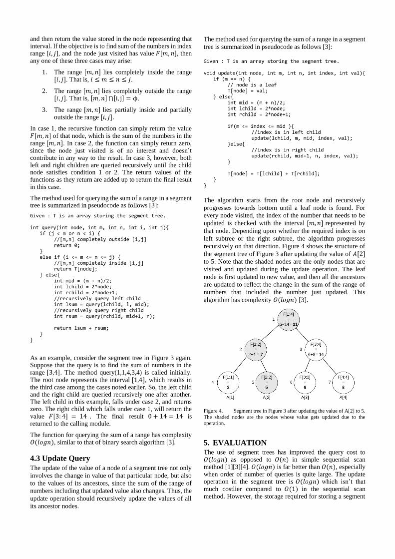
and then return the value stored in the node representing that interval. If the objective is to find sum of the numbers in index range [𝑖, 𝑗], and the node just visited has value 𝐹[𝑚, 𝑛], then any one of these three cases may arise:
1. The range [𝑚, 𝑛] lies completely inside the range [𝑖, 𝑗]. That is, 𝑖 ≤ 𝑚 ≤ 𝑛 ≤ 𝑗.
2. The range [𝑚, 𝑛] lies completely outside the range [𝑖, 𝑗]. That is, [𝑚, 𝑛] ⋂[i, j] = ϕ.
3. The range [𝑚, 𝑛] lies partially inside and partially outside the range [𝑖, 𝑗].
In case 1, the recursive function can simply return the value 𝐹[𝑚, 𝑛] of that node, which is the sum of the numbers in the range [𝑚, 𝑛]. In case 2, the function can simply return zero, since the node just visited is of no interest and doesn’t contribute in any way to the result. In case 3, however, both left and right children are queried recursively until the child node satisfies condition 1 or 2. The return values of the functions as they return are added up to return the final result in this case.
The method used for querying the sum of a range in a segment tree is summarized in pseudocode as follows [3]:
Given : T is an array storing the segment tree. int query(int node, int m, int n, int i, int j){ if (j < m or n < i) { //[m,n] completely outside [i,j] return 0; } else if (i <= m <= n <= j) { //[m,n] completely inside [i,j] return T[node]; } else{ int mid = (m + n)/2; int lchild = 2*node; int rchild = 2*node+1; //recursively query left child int lsum = query(lchild, l, mid); //recursively query right child int rsum = query(rchild, mid+1, r); return lsum + rsum; } }
As an example, consider the segment tree in Figure 3 again. Suppose that the query is to find the sum of numbers in the range [3,4]. The method query(1,1,4,3,4) is called initially. The root node represents the interval [1,4], which results in the third case among the cases noted earlier. So, the left child and the right child are queried recursively one after another. The left child in this example, falls under case 2, and returns zero. The right child which falls under case 1, will return the value 𝐹[3: 4] = 14 . The final result 0 + 14 = 14 is returned to the calling module.
The function for querying the sum of a range has complexity 𝑂(𝑙𝑜𝑔𝑛), similar to that of binary search algorithm [3].
4.3 Update Query
The update of the value of a node of a segment tree not only
involves the change in value of that particular node, but also
to the values of its ancestors, since the sum of the range of
numbers including that updated value also changes. Thus, the
update operation should recursively update the values of all
its ancestor nodes.
The method used for querying the sum of a range in a segment
tree is summarized in pseudocode as follows [3]:
Given : T is an array storing the segment tree. void update(int node, int m, int n, int index, int val){ if (m == n) { // node is a leaf T[node] = val; } else{ int mid = (m + n)/2; int lchild = 2*node; int rchild = 2*node+1; if(m <= index <= mid ){ //index is in left child update(lchild, m, mid, index, val); }else{ //index is in right child update(rchild, mid+1, n, index, val); } T[node] = T[lchild] + T[rchild]; } }
The algorithm starts from the root node and recursively
progresses towards bottom until a leaf node is found. For
every node visited, the index of the number that needs to be
updated is checked with the interval [𝑚, 𝑛] represented by
that node. Depending upon whether the required index is on
left subtree or the right subtree, the algorithm progresses
recursively on that direction. Figure 4 shows the structure of
the segment tree of Figure 3 after updating the value of 𝐴[2] to 5. Note that the shaded nodes are the only nodes that are
visited and updated during the update operation. The leaf
node is first updated to new value, and then all the ancestors
are updated to reflect the change in the sum of the range of
numbers that included the number just updated. This
algorithm has complexity 𝑂(𝑙𝑜𝑔𝑛) [3].
Figure 4. Segment tree in Figure 3 after updating the value of A[2] to 5.
The shaded nodes are the nodes whose value gets updated due to the
operation.
5. EVALUATION
The use of segment trees has improved the query cost to 𝑂(𝑙𝑜𝑔𝑛) as opposed to 𝑂(𝑛) in simple sequential scan method [1][3][4]. 𝑂(𝑙𝑜𝑔𝑛) is far better than 𝑂(𝑛), especially when order of number of queries is quite large. The update operation in the segment tree is 𝑂(𝑙𝑜𝑔𝑛) which isn’t that much costlier compared to 𝑂(1) in the sequential scan method. However, the storage required for storing a segment

tree is obviously larger than that required for a sequential array of numbers.
6. CONCLUSION
The use of segment trees while answering to range queries have drastically reduced the complexity of the query when the number of queries is in large order. Except the cases where there are very few query operation and very frequent update operations, or the cases where the memory usage is very critical, use of segment trees is the recommended way to answer to range queries.
7. REFERENCES
[1] J. Bentley and J. Friedman, "Data Structures for Range Searching", ACM Computing Surveys, vol. 11, no. 4, pp. 397-409, 1979. Available: 10.1145/356789.356797.
[2] "Segment Tree | Set 1 (Sum of given range) - GeeksforGeeks", GeeksforGeeks, 2018. [Online]. Available: https://www.geeksforgeeks.org/segment-tree-set-1-sum-of-given-range/. [Accessed: 2- Dec- 2018].
[3] "Segment Trees Tutorials & Notes | Data Structures | HackerEarth", HackerEarth, 2018. [Online]. Available: https://www.hackerearth.com/practice/data-structures/advanced-data-structures/segment-trees/tutorial/. [Accessed: 2- Dec- 2018].
[4] I. Setiadi, "Segment Tree for Solving Range Minimum Query Problems", 2012. Available: 10.13140/2.1.4279.2643.
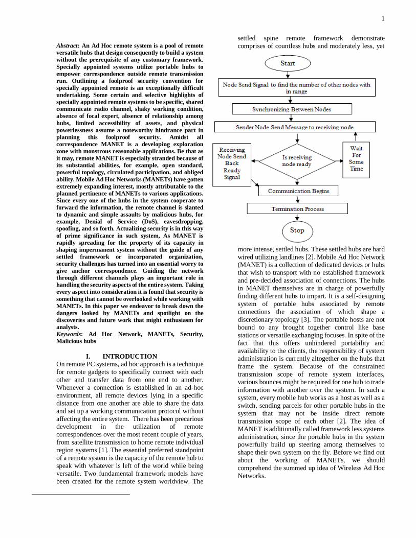
1
Abstract: An Ad Hoc remote system is a pool of remote
versatile hubs that design consequently to build a system
without the prerequisite of any customary framework.
Specially appointed systems utilize portable hubs to
empower correspondence outside remote transmission
run. Outlining a foolproof security convention for
specially appointed remote is an exceptionally difficult
undertaking. Some certain and selective highlights of
specially appointed remote systems to be specific, shared
communicate radio channel, shaky working condition,
absence of focal expert, absence of relationship among
hubs, limited accessibility of assets, and physical
powerlessness assume a noteworthy hindrance part in
planning this foolproof security. Amidst all
correspondence MANET is a developing exploration
zone with monstrous reasonable applications. Be that as
it may, remote MANET is especially stranded because of
its substantial abilities, for example, open standard,
powerful topology, circulated participation, and obliged
ability. Mobile Ad Hoc Networks (MANETs) have gotten
extremely expanding interest, mostly attributable to the
planned pertinence of MANETs to various applications.
Since every one of the hubs in the system cooperate to
forward the information, the remote channel is slanted
to dynamic and simple assaults by malicious hubs, for
example, Denial of Service (DoS), eavesdropping,
spoofing, and so forth. Actualizing security is in this way
of prime significance in such system, As MANET is
rapidly spreading for the property of its capacity in
shaping impermanent system without the guide of any
settled framework or incorporated organization,
security challenges has turned into an essential worry to
give anchor correspondence. Guiding the network
through different channels plays an important role in
handling the security aspects of the entire system. Taking
every aspect into consideration it is found that security is
something that cannot be overlooked while working with
MANETs. In this paper we endeavor to break down the
dangers looked by MANETs and spotlight on the
discoveries and future work that might enthusiasm for
analysts.
Keywords: Ad Hoc Network, MANETs, Security,
Malicious hubs
I. INTRODUCTION
On remote PC systems, ad hoc approach is a technique
for remote gadgets to specifically connect with each
other and transfer data from one end to another.
Whenever a connection is established in an ad-hoc
environment, all remote devices lying in a specific
distance from one another are able to share the data
and set up a working communication protocol without
affecting the entire system. There has been precarious development in the utilization of remote
correspondences over the most recent couple of years,
from satellite transmission to home remote individual
region systems [1]. The essential preferred standpoint
of a remote system is the capacity of the remote hub to
speak with whatever is left of the world while being
versatile. Two fundamental framework models have
been created for the remote system worldview. The
settled spine remote framework demonstrate
comprises of countless hubs and moderately less, yet
more intense, settled hubs. These settled hubs are hard
wired utilizing landlines [2]. Mobile Ad Hoc Network (MANET) is a collection of dedicated devices or hubs
that wish to transport with no established framework
and pre-decided association of connections. The hubs
in MANET themselves are in charge of powerfully
finding different hubs to impart. It is a self-designing
system of portable hubs associated by remote
connections the association of which shape a
discretionary topology [3]. The portable hosts are not
bound to any brought together control like base
stations or versatile exchanging focuses. In spite of the
fact that this offers unhindered portability and
availability to the clients, the responsibility of system administration is currently altogether on the hubs that
frame the system. Because of the constrained
transmission scope of remote system interfaces,
various bounces might be required for one hub to trade
information with another over the system. In such a
system, every mobile hub works as a host as well as a
switch, sending parcels for other portable hubs in the
system that may not be inside direct remote
transmission scope of each other [2]. The idea of
MANET is additionally called framework less systems
administration, since the portable hubs in the system powerfully build up steering among themselves to
shape their own system on the fly. Before we find out
about the working of MANETs, we should
comprehend the summed up idea of Wireless Ad Hoc
Networks.
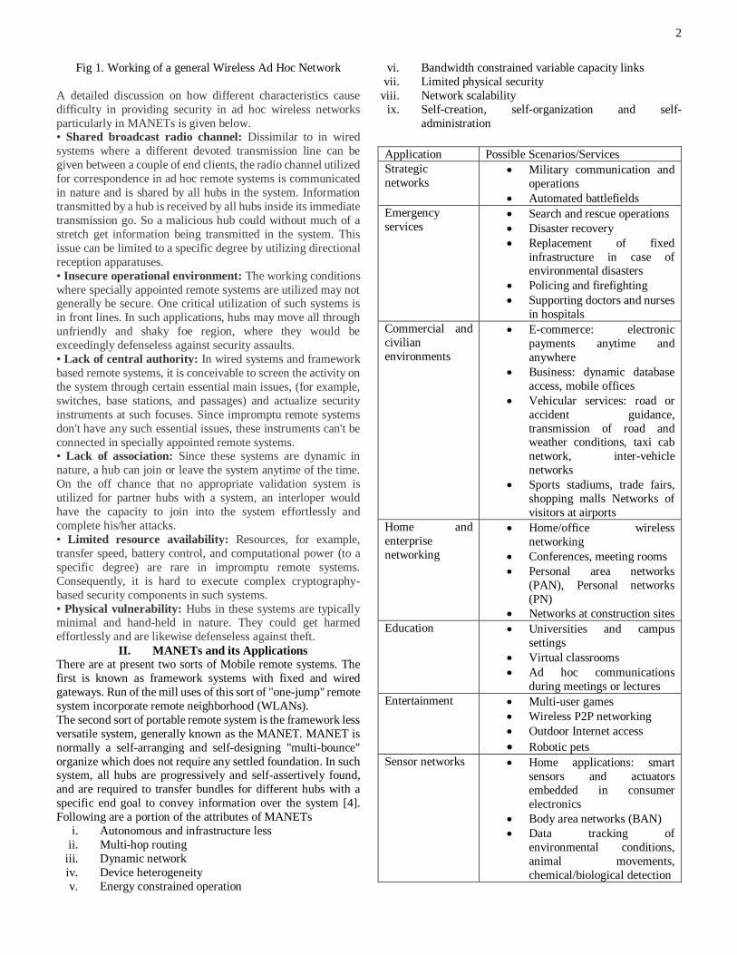
2
Fig 1. Working of a general Wireless Ad Hoc Network
A detailed discussion on how different characteristics cause
difficulty in providing security in ad hoc wireless networks
particularly in MANETs is given below. • Shared broadcast radio channel: Dissimilar to in wired
systems where a different devoted transmission line can be
given between a couple of end clients, the radio channel utilized
for correspondence in ad hoc remote systems is communicated
in nature and is shared by all hubs in the system. Information
transmitted by a hub is received by all hubs inside its immediate
transmission go. So a malicious hub could without much of a
stretch get information being transmitted in the system. This
issue can be limited to a specific degree by utilizing directional
reception apparatuses.
• Insecure operational environment: The working conditions
where specially appointed remote systems are utilized may not generally be secure. One critical utilization of such systems is
in front lines. In such applications, hubs may move all through
unfriendly and shaky foe region, where they would be
exceedingly defenseless against security assaults.
• Lack of central authority: In wired systems and framework
based remote systems, it is conceivable to screen the activity on
the system through certain essential main issues, (for example,
switches, base stations, and passages) and actualize security
instruments at such focuses. Since impromptu remote systems
don't have any such essential issues, these instruments can't be
connected in specially appointed remote systems. • Lack of association: Since these systems are dynamic in
nature, a hub can join or leave the system anytime of the time.
On the off chance that no appropriate validation system is
utilized for partner hubs with a system, an interloper would
have the capacity to join into the system effortlessly and
complete his/her attacks.
• Limited resource availability: Resources, for example,
transfer speed, battery control, and computational power (to a
specific degree) are rare in impromptu remote systems.
Consequently, it is hard to execute complex cryptography-
based security components in such systems.
• Physical vulnerability: Hubs in these systems are typically minimal and hand-held in nature. They could get harmed
effortlessly and are likewise defenseless against theft. II. MANETs and its Applications
There are at present two sorts of Mobile remote systems. The
first is known as framework systems with fixed and wired
gateways. Run of the mill uses of this sort of "one-jump" remote
system incorporate remote neighborhood (WLANs).
The second sort of portable remote system is the framework less
versatile system, generally known as the MANET. MANET is
normally a self-arranging and self-designing "multi-bounce"
organize which does not require any settled foundation. In such system, all hubs are progressively and self-assertively found,
and are required to transfer bundles for different hubs with a
specific end goal to convey information over the system [4].
Following are a portion of the attributes of MANETs i. Autonomous and infrastructure less
ii. Multi-hop routing
iii. Dynamic network
iv. Device heterogeneity
v. Energy constrained operation
vi. Bandwidth constrained variable capacity links
vii. Limited physical security
viii. Network scalability
ix. Self-creation, self-organization and self-
administration
Application Possible Scenarios/Services
Strategic
networks Military communication and
operations
Automated battlefields
Emergency
services Search and rescue operations
Disaster recovery
Replacement of fixed
infrastructure in case of environmental disasters
Policing and firefighting
Supporting doctors and nurses
in hospitals
Commercial and
civilian
environments
E-commerce: electronic
payments anytime and
anywhere
Business: dynamic database
access, mobile offices
Vehicular services: road or
accident guidance,
transmission of road and weather conditions, taxi cab
network, inter-vehicle
networks
Sports stadiums, trade fairs,
shopping malls Networks of
visitors at airports
Home and
enterprise
networking
Home/office wireless
networking
Conferences, meeting rooms
Personal area networks
(PAN), Personal networks
(PN)
Networks at construction sites
Education Universities and campus
settings
Virtual classrooms
Ad hoc communications
during meetings or lectures
Entertainment Multi-user games
Wireless P2P networking
Outdoor Internet access
Robotic pets Sensor networks Home applications: smart
sensors and actuators
embedded in consumer
electronics
Body area networks (BAN)
Data tracking of
environmental conditions,
animal movements,
chemical/biological detection
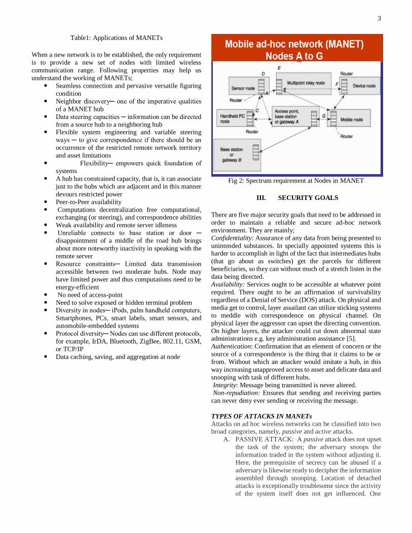
3
Table1: Applications of MANETs
When a new network is to be established, the only requirement
is to provide a new set of nodes with limited wireless
communication range. Following properties may help us
understand the working of MANETs;
Seamless connection and pervasive versatile figuring
condition
Neighbor discovery─ one of the imperative qualities
of a MANET hub
Data steering capacities ─ information can be directed
from a source hub to a neighboring hub Flexible system engineering and variable steering
ways ─ to give correspondence if there should be an
occurrence of the restricted remote network territory
and asset limitations
Flexibility─ empowers quick foundation of
systems
A hub has constrained capacity, that is, it can associate
just to the hubs which are adjacent and in this manner
devours restricted power
Peer-to-Peer availability
Computations decentralization free computational, exchanging (or steering), and correspondence abilities
Weak availability and remote server idleness
Unreliable connects to base station or door ─
disappointment of a middle of the road hub brings
about more noteworthy inactivity in speaking with the
remote server
Resource constraints─ Limited data transmission
accessible between two moderate hubs. Node may
have limited power and thus computations need to be
energy-efficient
No need of access-point
Need to solve exposed or hidden terminal problem Diversity in nodes─ iPods, palm handheld computers,
Smartphones, PCs, smart labels, smart sensors, and
automobile-embedded systems
Protocol diversity─ Nodes can use different protocols,
for example, IrDA, Bluetooth, ZigBee, 802.11, GSM,
or TCP/IP
Data caching, saving, and aggregation at node
Fig 2: Spectrum requirement at Nodes in MANET
III. SECURITY GOALS
There are five major security goals that need to be addressed in
order to maintain a reliable and secure ad-hoc network
environment. They are mainly;
Confidentiality: Assurance of any data from being presented to
unintended substances. In specially appointed systems this is harder to accomplish in light of the fact that intermediates hubs
(that go about as switches) get the parcels for different
beneficiaries, so they can without much of a stretch listen in the
data being directed.
Availability: Services ought to be accessible at whatever point
required. There ought to be an affirmation of survivability
regardless of a Denial of Service (DOS) attack. On physical and
media get to control, layer assailant can utilize sticking systems
to meddle with correspondence on physical channel. On
physical layer the aggressor can upset the directing convention.
On higher layers, the attacker could cut down abnormal state administrations e.g. key administration assistance [5].
Authentication: Confirmation that an element of concern or the
source of a correspondence is the thing that it claims to be or
from. Without which an attacker would imitate a hub, in this
way increasing unapproved access to asset and delicate data and
snooping with task of different hubs.
Integrity: Message being transmitted is never altered.
Non-repudiation: Ensures that sending and receiving parties
can never deny ever sending or receiving the message.
TYPES OF ATTACKS IN MANETs
Attacks on ad hoc wireless networks can be classified into two broad categories, namely, passive and active attacks.
A. PASSIVE ATTACK: A passive attack does not upset
the task of the system; the adversary snoops the
information traded in the system without adjusting it.
Here, the prerequisite of secrecy can be abused if a
adversary is likewise ready to decipher the information
assembled through snooping. Location of detached
attacks is exceptionally troublesome since the activity
of the system itself does not get influenced. One

4
method for defeating such issues is to utilize intense
encryption systems to scramble the information being
transmitted, consequently making it inconceivable for
busybodies to acquire any helpful data from the
information caught.
B. ACTIVE ATTACK: An active attack endeavors to
change or decimate the information being traded in the
system, in this manner disturbing the typical working
of the system. Dynamic attacks can be ordered further
into two classifications, to be specific, external and
internal attacks. External attacks are done by hubs that
don't have a place with the system. These assaults can
be anticipated by utilizing standard security systems,
for example, encryption strategies and firewalls. Internal attacks are from traded off hubs that are very
of the system. Since the enemies are now part of the
system as approved hubs, inner assaults are more
extreme and hard to identify when contrasted with
outer attacks.
Fig 3: Classifications of attacks
C. INTERNAL ATTACKS: Internal attacks are directly
leads to the attacks on nodes presents in network and
links interface between them [10]
Fig. 4: External and internal attacks in MANET
D. WORMHOLE ATTACK
In this attack, an attacker receives packets at one location in the
network and tunnels them to another location in the network where the packets are again injected into the network. This
tunnel between two colluding attackers is called a wormhole.
Wormhole is an attack on MANET routing protocols in which
similar nodes create an impression that two distant sections of
a MANET are connected through nodes that seem to be adjacent
but are actually distant from one another [7][8]. Due to the
broadcast nature of the radio channels the attacker can create a
wormhole even for packets not addressed to itself. In figure5
node A sends RREQ to node B and nodes X and Y are
infectious nodes having an out-of-band connection between
them. Node X tunnel the RREQ to Y, which is actual neighbor
of B. B gets two RREQ – A-X-Y-B and A-C-D-E-F-B. Though no harm is done if the wormhole is used properly for efficient
relaying of packets, it puts the attacker in a powerful position in
comparison to other nodes in the network which the attacker
can use in order to compromise the security of the network.
Fig 5: Wormhole Attack
E. BLACK HOLE ATTACK
In this attack, an infected node falsely advertises helping paths
e.g. shortest path or stable paths to the root node during the path
finding processor during the updating process in table- driven
routing protocols. The intention of these infected nodes could be to interrupt the path finding process or to distract the nodes
from reaching the destination. For instance, in AODV, the
attacker can send a fake RREP (counting a phony goal
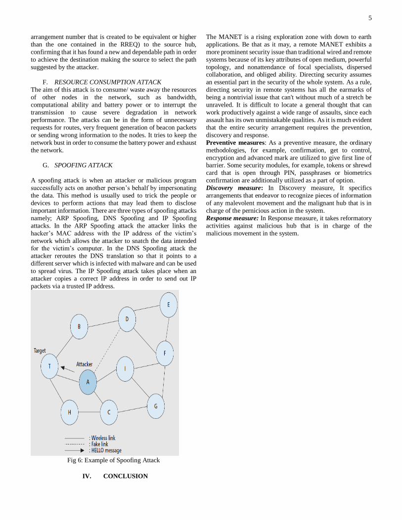
5
arrangement number that is created to be equivalent or higher
than the one contained in the RREQ) to the source hub,
confirming that it has found a new and dependable path in order
to achieve the destination making the source to select the path
suggested by the attacker.
F. RESOURCE CONSUMPTION ATTACK
The aim of this attack is to consume/ waste away the resources
of other nodes in the network, such as bandwidth,
computational ability and battery power or to interrupt the
transmission to cause severe degradation in network
performance. The attacks can be in the form of unnecessary
requests for routes, very frequent generation of beacon packets
or sending wrong information to the nodes. It tries to keep the
network bust in order to consume the battery power and exhaust
the network.
G. SPOOFING ATTACK
A spoofing attack is when an attacker or malicious program
successfully acts on another person’s behalf by impersonating
the data. This method is usually used to trick the people or
devices to perform actions that may lead them to disclose
important information. There are three types of spoofing attacks
namely; ARP Spoofing, DNS Spoofing and IP Spoofing
attacks. In the ARP Spoofing attack the attacker links the
hacker’s MAC address with the IP address of the victim’s
network which allows the attacker to snatch the data intended for the victim’s computer. In the DNS Spoofing attack the
attacker reroutes the DNS translation so that it points to a
different server which is infected with malware and can be used
to spread virus. The IP Spoofing attack takes place when an
attacker copies a correct IP address in order to send out IP
packets via a trusted IP address.
Fig 6: Example of Spoofing Attack
IV. CONCLUSION
The MANET is a rising exploration zone with down to earth
applications. Be that as it may, a remote MANET exhibits a
more prominent security issue than traditional wired and remote
systems because of its key attributes of open medium, powerful
topology, and nonattendance of focal specialists, dispersed collaboration, and obliged ability. Directing security assumes
an essential part in the security of the whole system. As a rule,
directing security in remote systems has all the earmarks of
being a nontrivial issue that can't without much of a stretch be
unraveled. It is difficult to locate a general thought that can
work productively against a wide range of assaults, since each
assault has its own unmistakable qualities. As it is much evident
that the entire security arrangement requires the prevention,
discovery and response.
Preventive measures: As a preventive measure, the ordinary
methodologies, for example, confirmation, get to control,
encryption and advanced mark are utilized to give first line of barrier. Some security modules, for example, tokens or shrewd
card that is open through PIN, passphrases or biometrics
confirmation are additionally utilized as a part of option.
Discovery measure: In Discovery measure, It specifics
arrangements that endeavor to recognize pieces of information
of any malevolent movement and the malignant hub that is in
charge of the pernicious action in the system.
Response measure: In Response measure, it takes reformatory
activities against malicious hub that is in charge of the
malicious movement in the system.
Related Documents


![PAPERS PUBLISHED IN PEER REVIEWED JOURNALSonline.gndu.ac.in/punjabi/pdf/AnnualReport_47/3 Papers Published in... · [142] PAPERS PUBLISHED IN PEER REVIEWED JOURNALS FACULTY OF ARTS](https://static.cupdf.com/doc/110x72/5f329b3077963314d010fdf1/papers-published-in-peer-reviewed-papers-published-in-142-papers-published.jpg)