NASA-CR-195734 DEVELOPMENT OF ROCKET MOTOR isor lUCCl eorge Aero_ ght Center _e nistration LOn 36849 (NASA-CR-195734) DEVELOPMENT OF A NEW GENERATION_SOLI D ROCKET MOTOR IGNITION COMPUTER CODE Final Report (Auburn Univ.) 173 p I N94-28800 Uncl -<°_ as -:7 G3/20 000261I _i i https://ntrs.nasa.gov/search.jsp?R=19940024297 2020-04-07T00:35:17+00:00Z

Welcome message from author
This document is posted to help you gain knowledge. Please leave a comment to let me know what you think about it! Share it to your friends and learn new things together.
Transcript

NASA-CR-195734
DEVELOPMENT OF ROCKET MOTOR
isor
lUCCl
eorgeAero_
ght Center_e nistration
LOn
36849
(NASA-CR-195734) DEVELOPMENT OF A
NEW GENERATION_SOLI D ROCKET MOTORIGNITION COMPUTER CODE Final Report
(Auburn Univ.) 173 p
I
N94-28800
Uncl -<°_a s -:7
G3/20 000261I _i
i
https://ntrs.nasa.gov/search.jsp?R=19940024297 2020-04-07T00:35:17+00:00Z

.I
=
m
k
:_ .............. 2 -- --,.T_r
T _ -: _
- - __ -- __
r

ABSTRACT
This report presents the results of experimental and
numerical investigations of the flow field in the head-end star
grain slots of the Space Shuttle Solid Rocket Motor. This work
provided the basis for the development of an improved solidrocket motor ignition transient code which is also described in
this report. The correlation between the experimental andnumerical results is excellent and provides a firm basis for the
development of a fully three-dimensional solid rocket motor
ignition transient computer code.
ii
Pi_IENN_ PAGE' BLANK NOT FILM_.D

ACKNOWLEDGEMENTS
The authors express appreciation to personnel of the George
C. Marshall Space Flight Center (MSFC) for their support and
assistance in this project. In particular, Mr. John E. Hengel,
whose overall support of this project was an essential factor inits overall success and to Mr. Andrew W. Smith for his technical
assistance. The authors also wish to thank to Mr. Billy H.
Holbrook for his work in constructing the experimental models.
iii

TABLE OF CONTENTS
ABSTRACT ................................................. i i
ACKNOWLEDGEMENTS......................................... i i i
LIST OF
LIST OF
FIGURES .......................................... v
TABLES ......................... _ ................. vii
NOMENCLATURE............................................... viii
I . INTRODUCTION ....................................... I_l
II. EXPERIMENTAL ANALYSIS .............................. II-i
Experimental Apparatus .............................. II-2
Test Facility ....................................... II-11
Test Plan ................... _ .... _,,.................. II-ll
Oil Smear Results .... II-12
Results From Static Pressure Measurements ........... II-13Results From Heat Transfer Measurements ............. II-13
References II-29
III. THEORETICAL/NUMERICAL ANALYSIS ...................... III-i
Introduction ........................................ III-i
Conservation Equations .............................. III-2
Turbulence Model .................................... III-6
Heat Transfer Relations ............................. III-8
Numerical Technique ............... . ................. III-10
Initial and Boundary Conditions ..................... III-ll
Sample Results ................. _ .................... III-13
References .......................................... III-23
IV. CAVENY PROGRAM MODIFICATIONS ........................ IV-I
References .......................................... IV-7
Vo CAVENY PROGRAM INTERFACE ............................ V-I
VI. XPLOT PROGRAM DESCRIPTION ........................... VI-I
VII. XPLOT USER
APPENDIX A
INSTRUCTIONS ............................. VII-I
Sample Caveny Input File. ........ , ...... A-I
APPENDIX B Caveny Program Makefile ................. B-I
APPENDIX C xplot Source Program .................... C-i
iv

LIST OF FIGURES
FIG. TITLE pAGE NQ
II-I
II-2
II-3
II-4
II-5
II-6
II-7
II-8
II-9
II-10
II-ll
II-12
II-13
II-14
II-15
II-16
II-17
II-18
II-19
II-20
II-21
II-22
II-23
II-24
II-25
II-26
II-27
II-28
II-29
II-30
II-31
II-32
II-33
II-34
II-35
II-36
II-37
II-38
II-39
II-40
II-41
II-42
II-43
II-44
II-45
II-46
II-47
Schematic of star slot ............................ II-4
Cross-section of star slot region ................. II-4
Schematic of head-end section ..................... II-8
Schematic of single-port and multi-port igniters..II-8
Head-end section model .......... .................. II-9
Igniters models ................................... II-9
Location of pressure taps and calorimeters ........ II-10Detail of
Igniter 1
Igniter 2
Igniter 3
Igniter 1
Igniter 2
Igniter 3
Igniter 1
Igniter 2
Igniter 3
Igniter 1
Igniter 2
Igniter 3
Igniter 1
Igniter 2
Igniter 3
Igniter 1
Igniter 2
Igniter 3
Igniter 1
Igniter 2
Igniter 3
Igniter i
Igniter 2
Igniter 3
Igniter 1
Igniter 2
Igniter 3
Igniter 1
Igniter 2
Igniter 3
Igniter 1
Igniter 2
Igniter 3
Igniter 1
Igniter 2
Igniter 3
Igniter 1
Igniter 2
Igniter 3
calorimeter installation ................ II-10
(i00 psi) .............................. II-14
(i00 psi) ........... . .................. II-14
(I00 psi) ......................... _-_..II-14
(500 psi) ................... .. .........................
(500 psi) .............................. II-15
(500 psi) .............................. II-15
(i000 psi) ............................. II-16
(i000 psi) ............................. II-16
(i000 psi) ............................. II-16
(1500 psi) ............................. II-17
(1500 psi) ............................. II-17
(1500 psi) ............................. II-17
(1800 psi) ............................. II-18
(1800 psi) ............................. II-18
(1800 psi) ............................. II-18
(i00 psi) .............................. II-19
(i00 psi) .............................. II-19
(i00 psi) .............................. II-19
(500 psi) ......... "..................... II-20
(500 psi) .............................. II-20
(500 psi) .............................. II-20
(I000 psi) ............................. II-21
(I000 psi) ............................. II-21
(I000 psi) ............................. II-21
(1500 psi)... .......................... II-22
(1500 psi> ............................. II-22
(1500 psi) ............................. II-22
(1800 psi) ............................. II-23
(1800 psi) ............................. II-23
(1800 psi) ............................. II-23
(100"psi) .............................. II-24
(i00 psi) .............................. II-24
(i00 psi) .............................. II-24
(500 psi) .............................. II-25
(500 psi) ...... ........................ II-25
(500 psi) .............................. II-25
(i000 psi) ............................. II-26
(1000 psi) ............................. II-26
(i000 psi) ............................. II-26
v
.FIG. TITLE pAGE _NO.
II-48
II-49
II-50
II-51
II-52
II-53
III-I (a)
III-i (b)
III-2
III-3
III-4
III-5
III-6
III-7
III-8
III-7
III-10
III-ll
III-12
VI-I
VI-2
VI-3
VI-4
VI-5
VII-I
VII-2
VII-3
VII-4
VII-5
VII-6
VII-7
VII-8
VII-9
VII-10
VII-II
VII-12
VII-13
VII-14
VII-15
VII-16
VII-17
VII-18
Igniter
Igniter
Igniter
Igniter
Igniter
Igniter
1 (1500 psi) ............................. II-27
2 (1500 psi) ............................. II-27
3 (1500 psi) ............................. II-27
1 (1800 psi) ............................. II-28
2 (1800 psi) ............................. II-28
3 (1800 psi).. ........................... II-28
Space shuttle SRM ................................. III-3
SRM star grain cross section... ................... III-3
SRM star grain calculation domain ................. III-3
Computational grid ................................ III-12
Space Shuttle SRM igniter flow vs. time trace ..... III-12
Igniter flow-field comparison (cold flow) ......... III-15
Single port igniter co_d'flow, Pi_i_,r = 6.8 atm .... III-1645 degree igniter cold-flow, P..?---- 6.8 atm......III-17
Single port Ignlter cold-flow, _. .L = 34 atm ..... III-18, , igniter
45 degree ignlter cold-flow, Pi_t_r = 34 atm ....... III-19
Typical slot area burn sequence'-(p-redicted) ....... III-20
Calculated Nu Contours (cold flow) single
port igniter ............. .,_._.,. ................... III-21
(Early) Ignition transient head-end pressure rise. III-22
Two-dimensional data organization ................. VI-4
One-dimensional data organization ................. VI-5
X toolkit application design model ................ VI-6
Plot layout design ........... , .................... VI-8
Example dialog diagram ............................ VI-12
xplot top level dialog ............................ VII-I
xplot input file editor dialog .................... VII-2
xplot execution setup dialog ...................... VII-4
Plot manager dialog ............................... VII-6
xplot format dialog .... .,.,.. ..................... VII-7
xplot data attributes dialog ...................... VII-10
xplot file editor dialog .......................... VII-II
xplot view dataset dialog ......................... VII-12
Pressure versus location at time=30 ms ............ VII-17
Pressure versus location at time=60 ms ............ VII-17
Pressure versus location at time=90 ms ............ VII-18
Pressure versus location at time=120 ms ........... VII-18
Pressure versus time at distance=3 cm ............. VII-20
Pressure versus time at distance=1330 cm .......... VII-20
Mach number & burn rate versus distance at
time=90 ms ........................................ VII-21
Mach number & burn rate versus distance at
time=180 ms ....................................... VII-22
Reynolds number at exit versus time ............... VII-23
Motor thrust versus time .......................... VII-23
vi
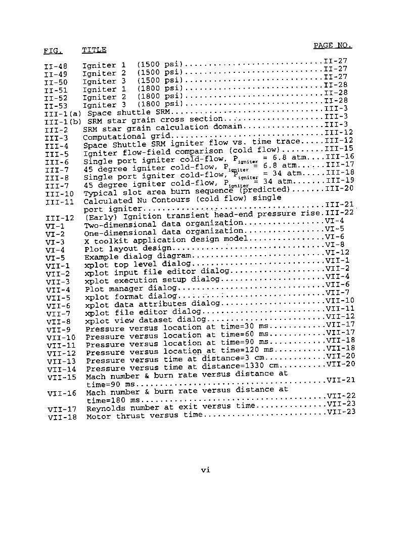
LIST OF FIGURES
Table _ PAGE NQ_
II-i
III-i
III-2
IV-I
IV-2
IV-3
IV-4
IV-5
IV-6
IV-7
IV-8
IV-9
VI-I
VI-2
VI-3
VII-I
VII-2
VII-3
VII-4
VII-5
VII-7
VII-8
VII-9
VII-10
Test matrix ...................................... II-i
Constants used in burning rate law ............... III-9
Solid propellant properties ...................... III-!0
Sample burning perimeter fraction table .......... IV-3
Caveny code input tables ...... .................... IV-3
Circular perforated grain variables .............. IV-4
Slotted grain variables .......................... IV-4
Star grain variables ........ ..................... IV-4
Wagonwheel grain variables ....................... IV-5
Dogbone grain variables .......................... IV-5
Sample burning geometry table .......... IV-5
Variables saved in caveny.plot file .............. IV-6
Widgets used in xplot ............................ VI-II
xplot source files ............................... VI-14
xplot header files ............................... VI-14
Input file editor dialog commands ................ VII-4
Execution dialog commands ............ .. .VII-5
Plot manager dialog commands ..................... VII-6
Format dialog commands .......... ,,, .............. VII-9
File editor dialog commands ...... _,_.,.,. ........ VII-!2
Command-line interface verbs ..................... VII-14
Xplot.clr file format ............................ VII-15
Xplot.var file format ............................ VII-15
Sample xplot.def file ............................ VII-16
vii

NOMENCLATURE
bCl, C2cpee_hckKMNuPPrrReStTU,V,WVx,y, z
7E
Ok, (_E
ep
= star slot width
= empirical constants appearing in turbulence model
= specific heat
= gas internal energy
= internal energy of the gaseous burning propellant= convective heat transfer coefficient
= kinetic energy of turbulent velocity fluctuations
= thermal conductivity
= Mach number
= Nusselt number
= pressure= Prandtl number
= propellant burn rate
= Reynolds number
= source term(s) in governing conservation equations
= time
= temperature
= velocity components
= (u2 + v2)_= spatial coordinates
= thermal diffusivity
= ratio of specific heats
= rate of dissipation of turbulent kinetic energy
= constants appearing in turbulence model
= constant appearing in propellant burn rate equation
subscripts
c = mass
e = energyi = initial value
= laminar
P = propellant
ref,R = reference condition
star tip = propellant grain star tip
t = turbulent
wa = adiabatic wall
xm,ym = x,y components of linear momentum
suDerscript
= dimensionless quantity
viii


I. INTRODUCTION
This report describes the results obtained from experimental
and numerical analyses conducted for the purpose of developing an
improved solid rocket motor ignition transient code. The
specific objective of this work was to improve ability to predict
the influence of the star grain on the ignition transient; in
particular, the calculation of the flame spreading rate on the
propellant surfaces inside the star slot_ This report is divided
into three main subject areas: i) e_erimental analysis, 2)
numerical analysis and 3) computer code modification, development
and documentation.
Section II presents the results of a series of experiments
conducted at NASA's George C. Marshall Space Flight Center
(MSFC). These experiments utilized a model designed and
constructed in the Aerospace Engineering Department at Auburn
University. This model is a one-tenth scale simulation of the
Space Shuttle Solid Rocket Motor (SRM) head-end section. The
model was tested in the special test section of the 14"x14"
trisonic wind tunnel at MSFC. The tests were cold-flow, using
air, simulations of the internal flow through the igniter nozzle
and the head-end section of the SRM. The air was supplied
through a special high pressure line connected to the wind
tunnel. There was no external flow around the model. The tests
were designed to provide both qualitative and quantitative data
on the interaction between the igniter plume and the star slots
and the flow field within the star slots. Qualitative
measurements were made using oil smears, Schlieren photography
and by seeding the flow field with aluminum particles which were
illuminated with a laser system and recorded on video tape.
Quantitative measurements were made of the pressure distributionwithin a slot and of the heat transfer rates to the wall of a
slot. The correlation of the data between the various
experiments performed is excellent.
Section III provides the theoretical basis for the
Computational Fluid Dynamic (CFD) model which was developed to
analyze the flow field in a star slot and the results obtained
from the CFD analysis. The CFD model was verified using the
experimental data obtained from the cold flow tests described
above. The primary objective of the CFD model was to provide
data regarding the spread of the combustion process throughout
the star slots. Based on these calculations a burning surface
area versus time model is obtained for use in the ignition
transient performance model of an SRM. The results of the
analysis are compared to existing motor data and are shown to be
in good agreement.
Sections IV-VII describe the modifications, interface,
program description, and instructions for an improved ignition
I-i

transient computer code. The modifications and interface are toan existing one-dimensional ignition transient computer code.The code was chosen because it is well documented and provides anefficient means of implementing the modifications to the burningsurface versus time calculations as determined from the analysesdescribed above. The ability to account for the flame spreadingin the star slot of the head-end section represents a significantstep forward in the ability to accurately model the early portionan SRM's ignition transient. The last two sections describe thedevelopment of a pre- and post-processor for an ignitiontransient code. The code presented here uses a modified one-dimensional ignition transient code modified to account for the
flame spreading in the star slots to solve for the ignition
transient performance of an SRM. However, it would be relatively
straightforward to modify the current version of the code to use
a more sophisticated ignition transient model as a solver. The
computer code is currently implemented on a SUN workstation using
X-Windows. Instructions necessary for using the program in an X-
Windows environment are included in Section VII. A sample input
file and the code for the pre- and post-processor are included in
the Appendices.
The work described in this report provides an excellent base
for the development of a fully three-dimensional ignition
transient performance prediction code using CFD techniques. The
experimental database which has been generated from this work
provides significant new insight into flow field phenomena
occurring in the star slots of SRM's which have head-end star
grains and head-end igniters.
I-2

II. EXPERIMENTALANALYSIS
One of the primary limitations of existing ignition transientprediction computer codes is an overestimation of the ignitiondelay and departure of the predicted pressure-time history curvefrom measured data in the early part of the transient. One of thereasons for this is the lack of data on the flow field in star
grain sections of solid rocket motors._ The experiments described
in this section focused on the flow field in the star grain section
of the Space Shuttle solid rocket motor (RSRM). The purpose of the
experiments was to obtain a credible data base for the flow field
patterns and heat transfer rates within the star slots. A one-
tenth scale model of the Space Shuttle_RSRM head-end star grain was
designed and constructed for the experimental study. The
availability of experimental flow field data during the ignition
transient in solid rocket motors is very scarce. Conover I
conducted cold flow tests using a one-tenth scale model of the
Space Shuttle solid rocket motor's head-end star grain section.
Conover's tests used both a single port igniter, such as found on
the RSRM and a three port igniter. The series of tests included
Schlieren photographs of the igniter mounted in a plenum, oil smear
data, pressure data and heat transfer coefficient measurements.
Fifteen pressure ports were fitted !n_one side plate of a slot,while fifteen calorimeters to measure heat transfer coefficients
were located in another slot. The data were taken at pressure
levels from 100 to 1500 psi in I00 psi increments. The actual
Space Shuttle igniter operates at approximately 2000 psi. Limits
on the test facility prevented taking data at higher igniter
chamber pressures. The static pressure data obtained provide some
qualitative trends, but there was considerable scatter in the data
when the igniter chamber pressure exceeded II00 psi. This was
probably due to the fact, as Conover states, that "above this
pressure the side plates used to form the star grain slots were
deflected to produce a one-sixteenth-inch gap where the plates come
together at the star points," thus causing some leakage. There
were also some apparent inconsistencies in the temperature data due
to model warm-up during the test. However, the oil smear data
provide a good indication of the _recirculating flow pattern inside
a slot. Even though Conover's experimenta!idata provide useful
information on the flow field inside the star slot, they should be
considered preliminary innature, and a Starting point for a more
in-depth investigation.
The present work describes a series of tests directed toward
the collection of qualitative and quantitative data documenting the
main characteristics of the flow in the head-end section of a solid
rocket motor. In particular? thefo_owing objectives were to be
accomplished with the test progr_.
II-I
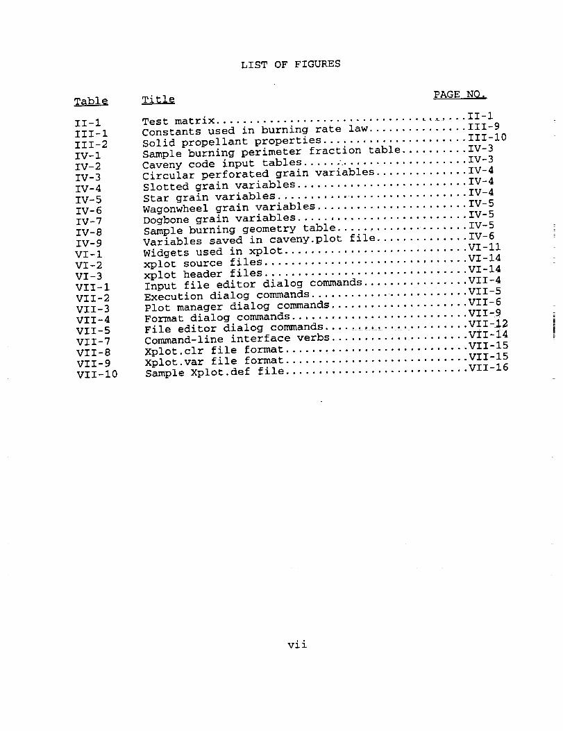
i) Obtain information on the igniter plume structure and
shape and its interaction with the star grain geometry.
2) Determine the region of the igniter
the side walls of the slots of
section model.
plume impingement on
the RSRM star grain
3) Determine the flow field characteristics of the subsonic,
recirculating flow within the slot.
4) Measure the heat transfer coefficients at several
locations inside the slot.
The above objectives were to be accomplished using the
following techniques:
i)
2)
Flow visualization.
Oil smears
3) Static pressure measurements
4) Heat transfer coefficient measurements
5) Velocity measurements
ExDerimenta! Apparatus
The test article used in this investigation was a one-tenth
scale, cold flow model based on the geometry of the Space Shuttle
RSRM head-end section. The test article had four slots, as opposed
to eleven slots in the actual Space Shuttle motor. A single port
igniter model and two four-port igniter models were used in the
tests. _ _
The scale factor of I:I0 was derived from an analysis_whihh
matches the Reynolds number between the model flow and the full
scale flow in the star grain section. Besides geometrical
similitude, the primary scaling parameter to ensure proper
similarity between the cold flow model and the real, full scale
motor is the Reynolds number. Compressibility effects are
important only in the igniter plume region, since the flow inside
a star slot is essentially subsonic. However, the igniter mass
flow rate is an important parameter, since it is thought to be
responsible for entrainment of the flow, which de_ermines the
recirculation pattern. The value of the Reynolds number determinesthe nature of the viscous effects. The viscous effects in turn are
related to the local convective heat transfer coefficient and
therefore to the amount of heat transfer from the hot gases to the
solid propellant. An exact match of Reynolds number between the
model and full scale flow field is not necessary for similarity.
Instead, generally good agreement between Reynolds numbers is a
sufficient condition for the general studies of these flow fields,
II-2

as has been extensively documented in theliterature. 2-s
Because of the complicated nature of the flow in the head-endsection, it is difficult to define an overall Reynolds number forthe entire slot. However, it seems appropriate to consider arepresentative Reynolds number, which can be defined at any pointin the star slot, as:
pVLa z --
II-i
where _ V and _ are the local density, velocity and viscosity,respectively, and L is a geometric reference length (for instance,
the distance from a given point to the motor centerline). The
product pV can be viewed as the local mass flux. It is assumed
that this local mass flux is proportional to the overall mass flux
that enters a star slot, which in turn is proportional to the mass
flow rate that enters the star slot divided by the open area of the
slot, so that:
II-2
where b and 1 are the slot width and slot length, respectively, as
shown in Figure II-l.
The mass flow rate that actually enters a given slot depends
on several factors, such as igniter mass flow rate, _n , geometric, , Ig
dimensions of the slot and motor, and lgnlter plume shape. The
functional dependency between these parameters is usually not
known, but can be generally expressed as:
m.lo_ .ct = _io_ .vailf (pl ume/hape) Z I - 3
To simplify the analysis, it can be assumed that three-
dimensional effects are negligible and the mass flow available to
the slot, _n. ., is the portion Of igniter mass flow encompassed• , SIQt, avail
in the clrcuIar sector facing the same slot (see Fig. II-2), or
8 b II-4
The factor b/(2 _) can be considered as the fraction of the port
perimeter occupied by a slot.
Using Eqs. (II-2), (II-3) and (II-4), the Reynolds number can
be expressed as: : _ _
II-3

I,
b
Fig. II-i Schematic of star slot
+
Fig. II-2 Cross-section of star slot region
II-4

R _ _ig L f[plumeshape)-" 2nr 111
II-5
Note that the Reynolds number, and thus the flow pattern inside the
slot, is independent of the number of slots.
For proper scaling,to the actual motor and 2
assumptions are made:
let Rel = Re2, where the subscript 1 refers
refers to the model. Then the following
i) All dimensions are exactly scaled.
2) The igniter plume shape is scaled for 1 and 2.
Note that the plume shape is determined mainly by the igniter
nozzle area ratio, igniter stagnation pressure, P , and backO
pressure. When all dimensions are scaled, the area ratlo is the
same for the real srm and the scaled model. The back pressure is
also the same, and equal to Lthe ambient value. This latter
condition is true at least until the point in time when a first
ignition occurs. This suggests that the igniter total pressure
ideally should be the same, that is 2000 psi.
Under the assumptions above, f(plume shape) drops out when
equating the Reynolds numbers, and the following relationship isobtained:
r24 q _
Then, defining the scaling factor as S, so that
II-6
S _II-7
Equation (II-6) is reduced to:
mlgl _2II-8
At this point, an appropriate viscosity-temperature relationship
must be chosen. Following Caveny 5, an empirical curve fit for
II-5

typical combustion gases is such that viscosity, _, is proportionalto the gas temperature, T, as
_1 = _ "6
so that Eq. (II-8) becomes:
s-migl (_22
II-9
II-10
Since t_ _that _i' TI and T 2 are known values, it appears from Eq. (II-10)scale factor, S, can be arbitrarily chosen simply by
varying the igniter model mass flow rate, ml • However the, g '
igniter throat area Is dependent on th_e sca_e factor to be
determined. Furthermore, the igniter chamber pressure should be
close to 2000 psi because of the assumption that the plume shape
does not change from the real motor to the scaled model. This is
more evident if Eq. (II-10) is rewritten in terms of stagnation
pressures and temperatures, as:
2 2(y_-1)
2 2 (y2-1)
Note that the term A'2/A'; is, itself, S 2.
For the cold-flow tests, the values of R 2 and Y2 for air arechosen for the model, and typical values of the temperatures are
T02 = 310°K, T 2 = 298°K. Since _ = P - 2000 psi, the pressureterm does not contribute to thevalue_f • Representative valuesof the variables for the flow in the head-end section of the actual
SRM are taken from Ref. 5.
Substituting in Eq. (II-ll), a value equal to 0.098 is
obtained for S, which is very close to the chosen scale factor
i:i0. Fortuitously, a one-tenth scale also defines a model size
which is close to the largest size that would fit in the dimensions
of the test section of the 14xl4-inch tunnel employed for the
tests.
The number of slots was determined based on different
criteria. According to the previous analysis, the Reynolds number
is independent of the number of slots. Therefore, one can ideally
choose any convenient number. Even though the actual SRMhead-end
II-6

section has eleven slots, only four slots are used in the scaledmodel. This represents a tradeoff between the desirability of flowvisualization in one (transparent) star slot and the requirementsfor all other test instrumentation.
The entire star grain section model, as well as the threeigniter models, were fabricated from aluminum, except for thetransparent slot which consists of two plexiglas plates. The totallength of the model is 19.72 inches; the largest diameter is 16inches. Figures II-3 and II-4-show a schematic representation ofthe entire model and of the igniters, respectively.
Each star slot is formed from two plates separated by a bottomspacer of suitable thickness. _ insert at the head-end simulatesthe actual grain surface. Thecircular port is formed from fourcontoured pieces connected to the outer surface of the slot plates.Two plates are located at the upstream and downstream end to closethe slots, and provide the attachment points for all the parts.The igniter is connected to the inner surface of the head-endplate. The single port igniter has a insert into which the nozzle
has been cut. The single port igniter has a throat diameter of
0.6025 inches and a conical shape with a half-angle of 27.2
degrees. The area ratio is 1.428, The four-port igniters are
simply four straight holes drilled in the igniter casing, each with
a 0.3012 diameter. The four-port igniters are oriented so that
each of the four jets centerlines are directed into a star slot.
Figure II-5 shows the whole star grain section model. The three
igniters used are shown in Fig. Ii-6,
The model is fully instrumented for measuring the parametersof interest as defined above.
Static pressure measurements are taken inside a single star
slot and along two of the four contoured sectors forming the
circular port of the model. Three pressure ports are located along
each of the two contoured sectors. Twenty-eight static pressure
ports are provided in one wall of a star slot. The measurements
are taken at three different slot depths and consist of eight, ten,
and eight pressure taps, respectively, as shown in Fig. II-7. The
three depths are equally spaced along the height of the slot.
In the plate forming the wall adjacent to the one containing
the pressure taps, twenty-eight calorimeters are installed to
obtain heat transfer coefficient data. The calorimeters are placed
at the same geometric locations as the pressure ports (Fig. II-9).
Each calorimeter is mounted in a plug, flush with the inner surface
of the slot plate. A detail of the calorimeter installation is
given in Fig. II-8. In order to get accurate measurements of the
heat transfer coefficients, the calorimeters were pre-heated before
each measurement was taken.
A second star is used to obtain oil smear data. A silicone-
II-7

Fig. II-3 Schematic of head-end section
_2/// //// ////!_
/._,/// / 2 2/ // / /.:_,.z/ / //////_//" "
= .
Fig. II-4 Schematic of single-port and multi-port igniters
II-8

Fig. II-5 Head-end section model
Fig. II-6 Igniter models
II-9
Fig. II-7
Fig. II-8
Location of pressure taps and calorimeters
' _= "
,'s
Detail of calorimeter installation
II-10

based oil was used to apply a matrix of oil drops to the finished
surface of one of the plates in the slot. After each run, well
defined marks or smears indicated the local direction of the flow
and gave a good overall picture of the flow field.
The transparent slot previously mentioned was used for real
time flow visualization. A laser sheet was projected from the
aft-end of the model and illuminatedmost of the transparent
slot. Aluminum particles mixed with pure alcohol were injected
into the slot and the aluminum particles were illuminated by the
laser sheet. The movement of the particles was clearly visible
in the transparent slot and provided an excellent qualitative
measurement of the behavior of the flow field in the slot. The
flow visualization obtained using the aluminum particles gave a
more detailed picture of the flow patterns in the slot than was
possible with the oil smears. In addition, the real time nature
of measurements provided a means for studying the dynamic
characteristics of the flow field. Video tape recordings of
these experiments were made to docu/ent the measurements.
The fourth slot was initially intended for making hot-wire
aneometry measurements. However, because of difficulties
associated with flow blockage in the small slot and difficulties
in making measurements in or near the high speed (high subsonic
or low supersonic) plume, this measurement was abandoned for the
present investigation.
Test Facility
The cold-flow tests used the special test section in the
NASA Marshall Space Flight Center 14x14-inch trisonic wind
tunnel. The tunnel operated as an _ntermittent blow-down wind
tunnel from storage pressure to atmospheric exhaust. The full
Mach number capability was not needed for the test program which
was carried out. Instead only a high pressure internal flow
through the special test section was required. The high pressure
air passed through the hollow centerbody of the tunnel, into a
pipe connected to the head-end plate of the model. It was then
exhausted into the special test section through the igniter
models. There was no externa! fIow around the model. A venturi
was installed upstream of the model to determine the mass flow
rate through the igniter. Additional information regarding the
NASA/MSFC trisonic wind tunel is given in Ref. 6.
Test Plan
The test program included two main series of tests.
Table II-i shows the test matrix which was used for each series
of tests. In the first series each igniter model was placed in
the test section without the star grain portion of the model.
Air flow at pressures of 100, 500, _I000, 1500 and 1800 psi passed
through each of the igniters used in the experiments and mass
II-ii
flow rates corresponding to each pressure were recorded. ASchlieren system and video tape recorder were used during eachrun to examine the plume shape'at various pressures. This wasdone to establish a reference for the plume geometry which couldbe compared with the plume geometry observed with the star grain
in place.
The second series of tests used the entire head-end section
model along with each of the three igniters. Oil smear, flow
visualization, static pressure and heat transfer coefficient
measurements were made at each condition shown in the test matrix
of Table II-l. It should be noted that the test condition at
1800 psi approximates the design condition of 2000 psi at which
simlitude between the one-tenth scale model and the actual Space
Shuttle RSRM flow field is achieved. The value of 1800 psi was
used because it represents the upper limit on the facility at the
mass flow rates necessary for the tests.
Table II-l. Test matrix
Igniter Chamber i00 500 i000 1500 1800
Angle Pressure
(deg) (psi)
0 1 2 3 4 5
22.5 6 7 8 9 10
45 II 12 13 14 I 15|
Oil Smear Test Results
Oil smears were taken for each of the fifteen test
conditions shown in Table II-l. The oil smears were generated
from a pattern of oil droplets placed on one side of a slot. The
spacing between the droplets was approximately one-half inch.
Figs. II-9 through II-23 show photographs of the oil smears
generated for each of the fifteen test conditions. The oil
smears provide considerable detail regarding the direction of the
primary flow in the slots, the region of the igniter plume
impingement, and the recirculation patterns which occur in the
slot. Although qualtitative in nature, this data showed-good "
agreement with the data from the CFD analyses presented in refs.
7-9, which are summarized i n Section III of this report.
II-12

Results From Static Pressure Measurements
Static pressure measurements were made at 27 locations on
the surface of one of the slots. Fig. II-7 shows the location
and numbering scheme used for the static pressure ports. Static
pressure distributions obtained from these measurements are shown
in Figs. II-24 through II-38. This data confirms the
quantitative data obatained from the oil smear tests with regard
to the location of the main, f_w - pa_rs, recirculation regions,
stagnation points and "dead_ir_gions within the slot. The data
obtained agrees well with the CFD resuits which will be discussed
in Section III, where a compirison_will be given between the
experimetal data and the CFD results
Results From Heat Transfer Measurements
Calorimeters were placed in a slot face adjacent tO the slot
face where the static pressure measurements were made. The
calorimeters were located at points corresponding to the 27
locations shown in Fig. II-7. Because of the lack of asufficient number of calorimeters to measure data at all 27
locations simultaneous!y, two runs were made using 15calorimeters in each run. Three calorimeters were not moved
between runs to insure that consistent data were being obtainedbetween the two runs. _ The r4sults_for the measured heat transfer
coefficients are Sh0_ in F_g_._39-thr0ugh II-53.
II-13

Fig. II-9 Igniter 1 (i00 psi)
Fig. II-10 Igniter 2 (I00 psi)
Fig. II-ll Igniter 3 (I00 psi)
II-14

Fig. II-12 Igniter 1 (500 psi)
Fig. II-13 Igniter 2 (500 psi)
Fig. II-14 Igniter 3 (500 psi)
II-15

7
Fig. II-15 Igniter 1 (10.00 psi)
Fig. II-16 Igniter 2 (I000 psi)
N! _
Fig. II-17 Igniter 3 (i000 psii
II-16

Fig. II-18 Igniter 1 (1500 psi)
Fig. II-19 Igniter 2 (1500 psi)
Fig. II-20 Igniter 3 (1500 psi)
II-17

Fig. II-21 Igniter 1 (1800 psi)
Fig. II-22 Igniter 2 (1800 psi)
Fig. II-23 Igniter 3 (1800 psi)
II-18

Measured Pressure, Single Port Igniter
Pionl_erm_
i!,qi.
Fig. II-24 Igniter 1 (i00 psi)
Measured Pressure, 22 deg Igniter
PIonlu.": 100 psi
1-"
Fig. II-25 Igniter 2 (i00 psi)
Measured Pressure, 45 deg Ignller
P_..or : 1O0 psi
Fig. II-26 Igniter 3 (i00 psi)
II-19

Measured Presure, Single Port Ignller
1__ _B____ _p_nN_r: 500
j-Fig. II-27 Igniter 1 (500 psi)
Measured Pressure, 22 dog Igniter
I:bnltor = 500 psi
%.
Fig. II-28 Igniter 2 (500 psi)
Moesured Pressure, 45 deg IgnNer
Pion.w ,=1 O0 psi
Fig. II-29 Igniter 3 (500 psi)
II-20

Meaeured Pressure, S/n_g!ePort Igniter
Fig. II-30 Igniter 1 (i000 psi)
Measured Pressure, 22 deg Igniter
P_lw • 1000 psi
i:l!
Fig. II-31 Igniter 2 (1000 psi)
Meaeured Pressure, 45 (leg Igniter
Pb.,w .. 1000 psi
Fig. II-32 Igniter 3 (1000 psi)
II-21

Measured Pressure, Single Port Igniter
. P_n.q.: 1500
Fig. II-33 Igniter 1 (1500 psi)
Measured Pressure, 22 dog igniter
Fig. II-34 Igniter 2 (1500 psi)
Measured Pressure, 4S deg Igniter
Fig. II-35 Igniter 3 (1500 psi)
II-22

Measured Pressure, Single Porl Igniter
P_nlw = 1800 psi
i-
Fig. II-36 Igniter 1 (1800 psi)
Measured Pressure, 22 deg Igniter
I_.,,. ,. 1800 psi
Fig. II-37 Igniter 2 (1800 psi)
Measured Prenure, 45 deg Igniter
I
Fig. II-38 Igniter 3 (1800 psi)
II-23

Meaimred Heat Tr_mrrer. 8b_ole Port Ignher
Pm._ : 4.8 arm (1O0 psi)
J:|:
Fig. II-39 Igniter 1 (i00 psi)
f __ •
I:
%-
Fig. II-40 Igniter 2 (i00 psi)
Meuured Heal Tr_rmfor, 45_ Igniter
I%,_,,. U -tin (1O0psi)
-',_ _N....-'_.m. ,_._"_
Fig. II-41 Igniter 3 (100 psi)
II-24
I:
Fig. II-42 Igniter 1 (500 psi)
II.,l_b,. I,l_ pl
Fig. II-43 Igniter 2 (500 psi)
Im_pQwrw_ pml
!
Fig. II-44 Igniter 3 (500 psi)
II-25

Meuured Heel 'rrsnel'er.9ingle Port Igniter
PW.,.. - gOam, (1000 psi)
Fig. II-45 Igniter 1 (i000 psi)
Idea¢uredHe_Tr_e_w,_ Ig_ltsrP_,_. 1000pel
Fig. II-46 Igniter 2 (I000 psi)
Meuurecl He41tTrlnsfer. 45o Igniter_._.: M mlz. (1000 ps_
Fig. II-47 Igniter 3 (I000 psi)
II-26

M_ured Heel 'l_w, _nG_ Porl l(_Mmr
Ple_b. m1SOCIpel
!
I'_qD
Fig. II-48 Igniter 1 (1500 psi)
I%e,_, ,, 1100 Fel
Fig. II-49 Igniter 2 (1500 psi)
lleiwured Heel Trlv_w, 41_
Pll,,i,, ,, IlXW psi
Fig. II-50 Igniter 3 (1500 psi)
II-27

Measurod Heet Transfer, 8ingle Parl Ionll_'
!l
Fig. II-51 Igniter 1 (1800 psi)
Hut l_f_,, _, _._w
II_e.m_• 1144pei
Fig. II-52 Igniter 2 (1800 psi)
Ue.,u.,d X_ Tr..._.,, 46olgnNol,
P_h, = 12Z4 olin (lllO0 psi)
Fig. II-53 Igniter 3 (1800 psi)
II-28

References
Conover, G. H., Jr., "Cold-Flow Studies of Igniter Plume Flow
Fields and Heat Transfer," Final Report, NASA Grant No.
NGT-01-003-800, Auburn University, June 1984.
.
,
,
.
,
.
Schetz, J. A., Hewitt, P. A., and Thomas, R., "Swirl
Combustion Flow-Visualization Studies in a Water-Tunnel,"
Journal of Spacecraft and Rockets, Vol. 20, No. 6, Nov-Dec.,
1983, pp.574-582..
Schetz, J. A., Guruswamy, J., and Marchman, J. F., III,
"Effects of an S-Inlet on the Flow in a Dump Combustor,"
Journal of SPacecraft and Rockets, March-April, 1985, pp.
221-224.
Schetz, J. A., Sebba, F., and Thomas, R. H., "Flow-
Visualization Studies of a Solid Fuel Ramjet Combustor Using
a New Material-Polyaphrone," 22nd Joint Army, Naw, NASA, Air
Force Combustion Meetinq, October, 1985.
Caveny, L. H., and Kuo, K. K., "Ignition Transients of Large
Segmented Rocket Boosters," April 1976, NASA Contractor
Report CR-1501162, NASA George C. Marshall Space FlightCenter.
Simon, E., "The George C. Marshall Space Flight Center's
14xl4-Inch Trisonic wind Tunnel Technical Handbook,"
NASA TMX-53185, December, 1964.
Ciucci, A., Jenkins, R. M. and Foster, W. A., Jr.,
"Numerical Analysis of Ignition Transients in Solid Rocket
Motors," AIAA Paper 91-2426, 27 th AIAA/SAE/ASME Joint
Propulsion Conference, Sacremento, California, June, 1991.
.
.
Ciucci, A., "Numerical Investigation of the Flow Field in theHead-End Star Grain Section of a Solid Rocket Motor
During Ignition Transients," Ph.D_ Dissertation, Auburn
University, December, 1991.
Ciucci, A., Jenkins, R. M. and Foster, W. A., Jr., "Analysis
of Ignition and Flame Spreading in the Space Shuttle Head-End
Star Grain," AIAA Paper 92-3272, 28 _h AIAA/SAE/ASME/ASEE
Joint Propulsion Conference and Exhibit, Nashville,
Tennessee, July 6-8, 1992.
II-29

III. THEORETICAL/NID4ERICAL ANALYSIS
Introduction
The ignition transient of an SRM employing a pyrogen igniter
can be defined as the time interval from the onset of the igniter
flow to the time a quasi-steady flow develops. The starting
transient is traditionally divided into three phases: the induction
interval, or ignition lag; flame spreading; and chamber filling.
The induction interval begins when the igniter flow is initiated
and ends when a point on the propellant surface reaches a critical
ignition temperature, and a flame first appears. The flame
spreading phase follows, ending when the entire Propel!ant s_urface
is ignited. Following this is the chamber filling phase, during
which rapid chamber pressurization occurs due to the energy and
mass addition from the burning propellant. A peak pressure may
occur, followed by a pressure decrease towards an equilibrium
value, attained when mass production by the propellant equals the
mass outflow from the motor nozzle. Numerous studies have been
directed at the analysis of SRM ignition transient phenomena. As
discussed by Peretz,et al.*, these analyses can generally be
categorized into three groups: (I) lumped chamber parameter, P(t)
models2-_; (2) one dimensional, quasi-steady flow, P(x) modelsS,9;
and (3) temporal and one-dimensional flow field, P(x,t) models. 1,1°,n
The simplest analyses fall into the first group; a uniform chamber
pressure is assumed and an equation for dPc_r/dt is derived and
integrated to obtain a pressure-time trace. The flame spreading
speed is assumed to be a known constant. In P(x) type models, flow
property distributions are considered at each instant of time and
one-dimensional steady state conservation equations are solved
along the motor axis. As in the P(t) type models, the flame
spreading speed is not part of the solution but rather must be
input. In P(x,t) type models both spatial and temporal property
variations are considered. A series of control volume increments
are assumed along the motor axis and a set of time dependent one-
dimensional conservation equations are solved. The flame spreading
speed can be obtained as part of the solution if convective heat
transfer to the propellant grain is taken into account. A widely
used model of this type is that developed by Caveny and Kuo. I°
Jasper Lal,et a112, have recently developed a one-dimensional
model which takes canted pyrogen igniters into account by
modifying the heat transfer analysis to include direct igniter
plume impingement on the solid propellant surface Even more
recently, Johnston 13 has presented a numerical procedure for the
analysis of internal flows in a solid rocket motor wherein an
unsteady, axisymmetric solution of the Euler equations is combined
with simple convective and radiative fluid heat transfer models and
an unsteady one-dimensional heat conduction solution for the
propellant grain. Flow in the star grain slots is not directly
calculated. Instead, burn rate constants are adjusted to account
for the variable area in the star grain region. Results are
presented for a Titan 5_ segment SRM, a Titan 7 segment SRM, and
the Space Shuttle SRM. Of these three motors, the Space Shuttle
III-i

SRM has the more pronounced axial grooves in the star grain, andagreement of Johnston's model with pressure-time data in the head-end star grain section of this motor is acknowledged to be poor.
In general, it can be argued that predictions agree
quantitatively well with test data for motors such as those used on
the Space Shuttle, with the exception of the time period which
directly involves burning of the head-end star grain segment. It
may be argued that discrepancies arise primarily from three
factors: (i) the flow field is usually assumed to be one
dimensional; (2) the star geometry in the head-end segment is
approximated by variations in port area and burning perimeter of
the grain; and (3) the igniter flow field is not taken into
account. The present analysis seeks to address these issues.
Conservation Equations
In this investigation, the Space Shuttle solid rocket motor
(SRM) is taken as the reference motor design. It is characterized
by a large length-to-diameter ratio and by a small port-to-nozzle
throat area ratio. The reference motor is divided into four
segments, as shown in Fig. III-l(a). The head-end, star shaped
region of the solid propellant grain contains eleven slots; a cross
section of the head-end segment is shown in Fig. III-l(b).
The flow field to be analyzed is extremely complex; it is
unsteady, multi-dimensional, turbulent, and compressible. Further,
the flow field is divided into a supersonic core region, defined by
by the expanding gases from the igniter, and a subsonic region
inside the star slot. The two-dimensional, unsteady, compressible
Navier-Stokes equations, neglecting body forces and heat source
terms, are employed. The flow field is described by adopting a
cylindrical coordinate system for the port region from the motor
centerline to the star grain tips, and a rectangular cartesian
coordinate system for the region of the flow inside the star slot.
Although the flow-field is three dimensional in the head-end
section of the motor, the star grain cross sectional shape of the
propellant segment implies that a certain number of planes of
symmetry exist, so that it is possible to restrict the domain to
a single sector, as shown in Fig. III-2. The two-dimensional
Navier-Stokes equations are obtained by averaging the full,
three-dimensional Navier-Stokes equations (with a formal
integration) in a direction perpendicular to the plane of symmetry
of the star slot. Averaging is carried out along the azimuthal
coordinate,8 , in the port region, and in the z-direction inside
the star slot. The calculated flow field variables thus represent
an average value in the domain considered (area shaded in Fig. III-
2).
The governing equations can most conveniently be solved in
dimensionless form. For the flow under investigation, no "natural"
free stream parameters exist. Consequently, the values of the
igniter exit parameters at the condition of maximum igniter mass
flow have been chosen as reference conditions, with the distance
from the motor centerline to the bottom of the slot taken as the
III-2
Figure III-l: (a)Space Shuttle SRM; (b)SRM Star Grain Cross Section
\
A
%
Figure III-2:SRM Star Grain Calculation Domain
III-3
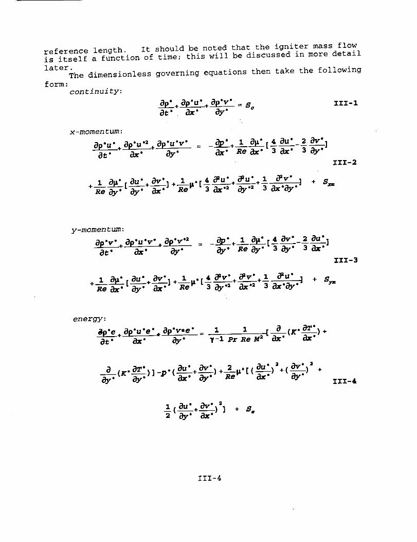
reference length. It should be noted that the igniter mass flow
is itself a function of time; this will be discussed in more detail
later.
The dimensionless governing equations then take the following
form:
continuity:
ap'÷ap.u.+a_p.v._ So i_i-1at • ax" ay"
x-momen tum :
a_p_.__/_+,gp'..,.2+ ap'u'v"at" ax" ay"
_ ap'. I a____.,4au"2av*,
III-2
+ I ap'[au'+av']+ I ..4t___+__+__u"_u" i _v- ] + s..
y-momen rum:
ap'v"+ ap'u'v"_ 8p'v"2at" az* ay"
_ap'+ i a_" 4 av* 2 au']
III-3
+ i a_" a,'+av" + i . _4_v'+_v'+1 _u" ] + s,.
energy:
• ap'v.e" 1 a (K" aT')÷ ap'u'e + ay" = 1_ [ +a:" T i px ae H= -_T -_-
ay'a(x..__.)]_p. (au"+_ ____.;_)av'+2__i,.[(ax'a"')=+(_ ')2+III-4
_l(au'+av') 2] + so2 o_" ax"
III-4

equations of state:
III-5
Ts
O ° =
¥ (¥-i)H 2IXI-6
The conservation equation source terms are given by:
III-7
_p'u*v" 2 1 @F' v'+ 1 yF[ 1 a tr'+o"u')S.. = y" --3 Re ax" y" Re (3 ax" o-)y"III-8
s,.= _p.v- _ _.ai,"v'._,___.___C(av'_v._y" 3 Re ay" y" 3 Re y, ay" y'"
III-9
1_I K" aT" . v" 2 o v" 2s.= - p'e'v'.y._rRe_,,=y.--_T-p7+-_-;P(-9_)
2 I . all" aV" V'. 2
-_-_l* (--÷--+--Jaz" ay" y"
III-10
for the circular port region of the computational domain.
slot itself, these terms are given by:
r •
For the
III-ll
III-5

2 I al," (A,' 2 i..au'.
s_ = -_ Re az" az"÷-bT-_ __ _z "j.III-12
2 I ap: aw'+ 2 i..av'.
s_,= -_-_-&_" az" -b-;_-&_P_=".III-13
where
2 . au',2+ av"
2 I ..au'+av" aw" 2+ A
er i(grain burning)
III-14
III-15
A i i 2 , ,'z'aT'_¥-1 Pr Re M _ b" az"
V
(no grain burning)III-16
Turbulence Model
The low Reynolds number form of the two-equation, k-£ model
developed by Jones and Launder 14'IS is used in the present analysis.
This model employs two variables, the kinetic energy of turbulent
velocity fluctuations, k, and the rate of dissipation of kinetic
energy, c, from which the turbulent viscosity, _t, is calculated.
The turbulent thermal conductivity, K t, is obtained by assuming a
constant value of the turbulent Prandtl number, o_=0.91. 16 The
turbulent kinetic energy and energy dissipation rate are determined
from the solution of the following differential equations:
k-equa tion :
aS__ + ap'u "k+ ap'v'k
at" az. ay.I a +l,_')m:]
- .___;1.___;_[(j,,"o k
I 1
1 . 2 . ak_)2+(_) 2] +S,III-17
III-6

£ -equa tion :
a_p/£+ ap'u'z + ap*v'z _at* ax" (,_," _-_T_{a [(p.+_) _____]+aax. _-T[(_,'+_')_.]}
1 e e _ 1 ._ 2 i,;i,__j[(ax "2 2+(ay "2+-_c_P_ +c_P2 _6c, p _ _e p. _u') _u')_]
_e p-- _-x ay" 2+2( .)2+2 (ax'y" ) + s.III-18
where
and
. 4 ( au')'÷(___.')2 a," av'] +( a,'+ av')2)P_--_(_[ az" ay -az'ay" ay" ax"
P2 = ---_p'k( au" + av" )az" ay"
III-19
III-20
The source terms are given by
= _P'v'k+ 1 (pi,+P=') ak i 2 .v"s_ (au'+av')ax . ay "
III-21
yV_ _" _ 1 2 c e . v" . au" av',III-22
in the circular port region of the domain, and by
s,=P. III-23
E
s, = c_;,,, III-24
III-7

_ 1 4 2 o_'au _o_'av']+( ) ( 2}P" _e I'_" {_[( ) a=" ax" az" _" a=
III-25
for the portion of the domain within theslot.
Heat Transfer Relations
The goal of the present analysis is to examine the interaction
between the igniter plume, the developing flow field within the
head-end star grain slots, and the rate of flame spread over the
grain surface. This, in turn, may provide insight into the
appropriateness of a particular grain design or a particular
igniter design for a given SRM. Many previous analyses utilize a
convection heat transfer model, while others, such as Johnston n,
utilize a combined convection-radiation model. The present
analysis utilizes a simple convection-only model developed by Kays
and Leung 17, and used previously to correlate heat transfer within
the O-ring gap of the Space Shuttle nozzle-to-case joint 18, given
by
0.152 Re °'p Pr/Vu= III-26
0.833[2.25 in(0.114 Re°'9)+13.2 Pr-5.8]
where the Reynolds number is based on the hydraulic diameter of a
single star grain slot. Fluid proper£ies are based on a "reference
temperature" denoted as 19
Tx = T + 0.5(T.n-_9 + 0.22(Twa-T9 III-27
and the adiabatic wall temperature is calculated from
T n = T+ sp_,._-_ V 2
2¢pIII-28
The propellant burning rate is assumed to be of the form
z = rro,(-P--)°exp[%(Tp-Tr.,) ]imz,_
III-29
The constants appearing in Eq.(27) are defined in Table III-l.
Erosive burning is assumed to be negligible during the very early
portion of the ignition transient.
III-8

Table III-l. Constants used in burning rate law
Cons tant Value Unit s
rr, _ 0.01078 m sec -I
Pr, f 6898.2 KPa
n 0.35 -
(_p 0. 002 K-I
Tref 300 K
_ _
In order to determine when a given element of the solid propellant
reaches a critical ignition temperature, one must know the surface
temperature of the solid grain. This, in turn, depends on the
amount of heat transferred to the grain from the hot gases.
The grain is considered to be a semi-infinite slab whose
temperature is initially uniform. Heat tranfer to th_ slab isassumed to be one-dimensional. Thus _k
=E/--L_ III-30at P 8z"
with the boundary conditions
a%!t,o hoTp(c,®) = To_ ; az - -_[T-T,(C, 0)]
fiX-31
and the initial condition
To(o, z) = Tp, III-32
The assumption of one dimensional conduction heat transfer implies
that ignition of adjacent grain surface elements is attributed to
direct heat transfer from the hot gas only. This appears to be a
reasonable assumption because of the low thermal conductivity of
the solid propellant. Assumed physical properties of the
propellant grain material are given in Table III-2.
III-9

Table III-2. Solid propellant properties
Property Value Units
pp 1758 Kg m "3
Kp 0.4605 W m "1 K -I
(cp)p 1256 J Kg -I K -I
Tp. critical 850 K
The initial propellant temperature is assumed to be Tpi = 298°K.
The (slot) wall shear stress must be approximated in order to
provide closure for the governing equations. A velocity profileacross the slot width (in the z-direction) is assumed for the
velocity components u and v. Pai°s 2° polynomial form of the
velocity profile for a flat duct is employed. For example, the u
component of velocity is
u
-I - P-q( z 2 ___ z 2;) - ( IXX-33
where uma x is the velocity at the symmetry plane of the duct (slot),
p = 11.06, and q = 162o . Although Eq.(III-33) applies specifically
to fully developed flow, it is used here to account for wall shear
stress effects even though the flow is time variant. It should be
noted that frictional effects at the slot walls are accounted for
only in the unignited portion of the propellant; they are
neglected for the ignited portion because of the strong transverse
velocity component due to mass injection from the burning
propellant.
Finally, the transverse velocity component w(z) is assumed to
be linear, with w = 0 at the slot plane of symmetry; w at the slot
wall can be determined from the known burning rate. Hence,
w. n = _ ; aw 2 III-34
Numerical Technique
The numerical solution of the equations of motion is obtained
utilizing the explicit, time-dependent, predictor-corrector finite
difference method developed by MacCormack. 21 This method has been
widely used for the numerical ....s6iution of a variety of fluid
III-10

dynamics problems, including those containing mixedsubsonic-supersonic flow regions, as in the present investigation.MacCormack's predictor corrector technique is well described in theexisting literature, n'n In the present investigation, an explicit,
fourth order numerical dissipation scheme has been introduced into
the set of equations to damp numerical oscillations induced by the
severe gradients in the flow field associated with the developing
igniter flow. The fourth-order damping scheme introduced by Holst 24
and modified by Berman 2s and Kuruvila 26 is employed. This scheme
involves certain free adjustable parameters, Cx and Cy, usuallyreferred to as damping or dissipation coefficients. It is
recommended in the literature n'n that C x, Cy be such that
0_Cx, Cy_0.5.- ...........A uniform rectangular grid is employed in the portion of the
domain that represents the head-end section, which includes the
star slot segment plus a distance equal to the port diameter. For
this region a 92x63 grid has been used, as shown in Figure III-3.
A grid of unequal spacing in the x-direction is used in the
extended portion of the domain from the head-end segment to the
motor exit. The scheme of Cebeci and Smith, 2_ in which grid spacing
is increased by a fixed percentage from an initial point, isutilized.
Initial and Boundary Conditions
In time marching problems, the initial conditions should in no
way affect the steady state results. In theory, any initial
conditions can be chosen. Of course, for an arbitrary set of
initial conditions, the transient has no physical meaning and only
the steady state condition is a meaningful representation of theflow field.
Since in this study the starting transient is of primary
importance, the initial conditions must reflect the actual values
of the flow field variables at time t = 0. Therefore, both
components of the velocity have been set equal to zero, u = v = 0,
and ambient values have been chosen for pressure and temperature
everywhere in the flow field. Density and internal energy are
obtained from the equation of state. The turbulent kinetic energy,
k, and its dissipation rate, £, are also zero initially. However,
imposing this value would lead to a singularity in the k and £
equations; thus, a very small value has been assigned to these two
variables.
Boundary conditions must also be specified for all of the
dependent variables, u, v, p, e, k, £, along with corresponding
values of p and T. Of primary importance is the specification of
the time variant conditions from the developing igniter flow at the
inflow boundary of the calculation domain. The conditions
specified are those from the single-port igniter used in the Space
Shuttle SRM. The igniter mass flow vs. time trace is shown in
Figure III-4, using data from Ref. 28. From the known igniter mass
flow rate vs. time trace and the geometry of the igniter nozzle,
the values of the flow variables u, p, p, T at the igniter nozzle
III-ll

...... - ....... ._ .;.,. ......
Figure III-3:Computational Grid
oo
O.J
160
140
120
100
$0
6O
40
2O
0
).00 0.0= 0.04 o.oe o.os 0._0 0.12 0.14 0._6 0.10 0=0TIME, seconds
Figure III-4: Space Shuttle SRM Igniter Flow vs. Time Trace
III-12

exit are calculated using one-dimensional nozzle flow theory; the
radial velocity is assumed to be zero, v=0, and the internal energy
is calculated from the known temperature. Note that the numerical
method employed is a shock capturing technique, so that the shock
waves associated with the igniter plume are embedded in the
solution. Inflow boundary conditions for k and £ must be also
specified. Since no experimentally measured profiles are
available, the turbulent kinetic energy is assumed to be equal to
a small percentage of the freestream kinetic energy, and the energy
dissipation rate is taken from an empirical relation used, for
instance, in Ref. 29. Along most solid walls of the computational
domain the "no slip" condition is enforced, that is, u = v = 0;
also, due to the low Reynolds Dumber form of the two-equation
turbulence model, k = 0 and £ = 0. For these walls the temperature
boundary condition is specified by assuming an adiabatic wall. The
exception is the cylindrical port portion of the domain downstreamof the star slot section. For this region, the wall temperature is
determined in the same manner as in the upstream star slot, and a
"blowing wall" (v _ 0) condition Is imposed to account for mass
addition due to burning. The top boundary of the computational
domain represents the centerline of the motor, so that a symmetry
boundary condition is enforced here.
The outflow boundary at the aft end of the motor represents
the final location where values of the dependent variables must be
specified. The approach adopted is to place a diaphragm at the
motor exit, immediately preceding a fictious "nozzle". When the
pressure differential across the diaphragm reaches some nominal
value, say 1 atm, the diaphragm bursts. The nozzle is assumed to
fill instantaneously. Continuous checks are made on the a m mount of
flow approaching the exit and the amount of flow the "nozzle" could
pass given the existing upstream conditions. A simple one
dimensional time-dependent mass conservation calculation is then
utilized to provide boundary conditions for the next time step. It
should be noted that, for the first 200 msec or so following
igniter firing, the downstream boundary condition is not as
important as it would be later in the ignition transient.
Sample Results
Cold Flow
After verification of the overall flow model and computational
technique by comparison with known solutions or measurements for
problems such as supersonic laminar flow over a flat plate _° and
developing turbulent flow in a pipe n, attention was turned to the
igniter plume as a measure of the model's ability to predict more
complex flow fields. Experimental data obtained both by Conover n
and in the series of tests described herein were utilized.
Schlieren photographs of the exhaust plume(s) were taken for each
igniter at various values of upstream total pressure. In
particular, the Space Shuttle SRM igniter is a single port, conical
nozzle configuration with an area ratio of 1.428 and a half angle
of 27.2 degrees, with a design exit Mach number of 1.79. Figure
III-13

III-5 compares the calculated plume Mach number contours for anigniter total pressure of 102 atm (1500 psi) and a totaltemperature of 316 °K with the Schlieren photograph of the plume atthe same conditions. A qualitive comparison indicates that the
results are quite satisfactory, although the shock wave appears to
be smeared over several grid points.
Next, calculations were performed for the cold flow (no
burning) flow field within the star slot of the head-end section.
The computed results can be compared with the oil smear data
obtained in the present cold flow tests. Both the case of a single
port igniter and a multi-port (canted) igniter are considered. The
multi-port igniter exhaust jet is aligned with the slot, at an
angle of 45 degrees with respect to the motor centerline. Typical
results are shown in Figures III-6:III-9. Figures III-6 and III-7
compare results for an igniter pressure of 6.8 atm (i00 psi), while
Figures III-8 and III-9 compare results for 34 atm (5.00 psi). The
igniter (not shown) is located near the upper right corner of the
slot, exhausting from right to left.
Hot Flow
Attention was next turned to the problem of heat transfer and
the calculated progression of the burning surface of the propellant
grain within the star slot. As time progresses, the propellant
surface temperature rises due to heat transfer from the hot gas
flowing over it. Propellant ignition is assumed to occur when the
temperature of the surface reaches a critical ignition temperature
(850 ° K) Obviously, the resulting flame spread is dependent on
the heat transfer correlation assumed (eg., Eq. III-26). Figure
III-10 illustrates a t ypica!predicted burn sequence for the single
port igniter presently used on the Space Shuttle SRM. First
ignition of the propellant surface occurs in the vicinity of the
shock located in the igniter plume, as might be expected.
Interestingly, this burnlng-progr-ession pattern can be anticipated
from calculated cold flow heat transfer contours, as can be seen in
Figure III-ll, which illustrates calculated Nusselt number contours
for cold flow over a range of igniter pressures from 6.8 atm (i00
psi) to 102 atm (1500 psi). Again, the igniter exhausts from right
to left.
Figure III-12 compares the calculated head-end pressure-time
trace with values obtained from measurements taken from actual
motor firings n, as well as with values calculated from a typical
P(x,t) model I°. The comparison is made for the time interval
0St_120 milliseconds, over which the first propellant grain
ignition occurs and flame spreading begins on the slot surface. It
can be seen that the P(x,t) model significantly underpredicts the
head end pressure during this interval, while the present model
matches the measured pressure trace with reasonable accuracy.
During this period, the flame spread is fairly slow, as would be
expected. A flame first appears on the propellant surface at 25
msec after the igniter firing, and at 120 msec approximately 20
percent of the star slot grain is burning. The rapid pressure rise
shown by the P(x,t) model at approximately 115 msec corresponds to
III-14

Figure III-5: Igniter Flowfield Comparison (cold-flow)
III-15

0il Smear
• ,- _ "_ ill i. ii=iiiii!:" -ili:!|i!iiiiiii!'l ' " ,. :, , i.:,,,'. ,, .,,,',:':,::,,:I
/llllli_-"_._,.,,_.i_.,j_ql"_"_.ii|-|=lil|/[ b_.'_.ii!ili::t.l:itl:,/llllll_l_ ___||!i:l:''!!/i!i|i/.ll.i:/ll::i i
i::===i::iiii!i!i,fl!i ..# .ili=ll ::!-,|- ti i:.--,,,,,--,,,-.....-,,_NGi '"ii" ,i1111!!i7 !II l,'l ....... , ........ l ..,...ii,..,i ill **,tli:;:::-: .i .... ii./ :I - --t--i ..I._ i -- ! I. ..i='ilii.: i-i- ": 11".1" ol I ,-*i. ,-,
/ii iiiiiiii=i:illlilt!i:!=!= :if= :i'l fi!'ii: ill#", , ,,::,,,,=,,=,,,i,,,,,,--,,,, -,,,,,,i,l.,,,,.,,.,,i i! iiiiil=
Oil Smear
_ _. .... ..._- .,;-: :- _ _ .: • .: "..: : .... -__'_..==_'--:;; r ; : ?: ::_.::._.
2 I I _ _ _ I _ I ° I | I ° I I : | I ; / : : :
:.:.''-:" 'I]i:,t:;1' !_i_!i_i_iiiiii_/'_l£__lll _ "_'
_ _,_ _ •.
i _iiii;.-!'': :: ::._.::_:.i_:::_._. ":=" *" ..! !"
Calculated
Figure III-7:45 Degree Igniter Cold-Flow, PL_,, = 6.8 atm
Ill-17

0il Smear
Calculated
Figure III-8: Single Port Igniter Cold-Flow, Ps_,, = 34 atm
Ill-18

011 Smear
1
.....",'""i0i, IIllI",i_ii'....
__, _ |I.F'_IIIIII!!_'
__HIIll ,
Calculated
Figure III-9:_5 De_ree I_nlter Cold-Flow, P_,, - 34 atm
IZI-19

I J
Figure III-10: Typical Slot Area Burn Sequence (predicted)
III-20

Cek::ulated (Cold Flow) Heat Transfer Contours
Igniter Pressure - 6.8 elm (100 psi)
J
Calculated (Cold Flow) Heat Transfer Contours
,goit.r,,e--or-r_:,_?oo_s)
Calculated (Cold Flow) Heat Transfer Contours
Igniter PreSSure -, 102 arm (1500 psi)
Figure III- II :Calculated Nu Contours (Cold-Flow) Single Port Igniter
III-21

100
90
80
70
60In,:3
50
0.
"0= 40
m
= 30
20
SRM Data
P(x,y) ModelPresent Model
/• ..._.l.
..,_o..
... °'°
10
0
0.00 0.02 0.04 0.06 0.08
time, seconds
0.10 0.12
Figure III-12: (Early) Ignition Transient Head-End Pressure Rise
III-22

the ignition of the CP portion of the grain in that model. First
ignition of the CP portion is predicted to be at approximately 80
msec in the present model. It should be noted that the present
model tends to under-predict the pressure rise in the head-end for
t > 120 msec. This suggests that the predicted flame spread for
time t > 120 msec is too low. This may be due to one or more of
several effects, including under-prediction of the convection heat
transfer coefficient, the presence of significant radiative heat
transfer, or the significance of 3-D conduction effects within the
propellant grain.
References
i , Peretz, A., et. ai., "Starting Transient of Solid-Propellant
Rocket Motors with High Internal Gas Velocities," AI____
Journal, Vol. ii, No. 12, December 1973, pp. 1719-1727.
.
.
DeSoto, S., and Friedman, H.A., "Flame Spreading and Ignition
Transients in Solid Grain Propellants_" AIAA Journal, Vol. 3,
March 1965, pp. 405-412.
Sforzini, R.H., and Fellows, H.L., Jr., "Prediction of _
Ignition Transients in Solid Propellant Rocket Motors,"
Journal of Spacecraft and Rockets, Vol. 7, No. 5, May 1970,
pp. 626-628.
. Sforzini, R.H., "Extension of a Simplified Computer Program
for Analysis of Solid-Propellant Rocket Motors," NASA CR-
129024, Auburn University, AL, April 1973 .......
. Caveny, L.H., and Summerfield, M., "Micro-Rocket Impulsive
Thrusters," Aerospace and Mechanical Science Rept. 1014,
November 1971, Princton, N.J.
. Bradley, H.H., Jr., "Theory of a Homogeneous Model of Rocket
Motor Ignition Transients," AIAA Preprint No. 64-127, January
1964.
. Most, W.J., and Summerfield, M., "Starting Thrust Transients
of Solid Rocket Engines," Aerospace and Mechanical Science
Report No. 873, July 1969, Princeton University, N.J.
. Threewit, T.R., Rossini, R.A., and Uecker, R.L., "The
Integrated Design Computer Program and the ACP-II03 Interior
Ballistics Computer Program," Rept. No. STM-180, Aerojet-
General Corp., December 1964.
, Vellacott, R.J., and Caveny, L.H., "A Computer Program for
Solid Propellant Rocket Motor Design and Ballistics Analysis,"
ARS Preprint No. 2315-62, January 1962.
III-23

I0. Caveny, L.H., and Kuo, K.K., "Ignition Transients of Large
Segmented Solid Rocket Boosters," Final Report, NASA CR-
150162, April 1976.
II. Caveny, L.H., "Extension to Analysis of Ignition Transients of
Segmented Rocket Motors," Final Report, NASA CR-150632,
January 1978.
12. Jasper Lal, C.,et. al., "Prediction of Ignition Transients in
Solid Rocket Motors Employing Cahded Pyrogen Igniters,"
Journal of Propulsion and Power, Vol. 6, No. 3, May-June 1990,
pp. 344-345.
13. Johnston, W.A., "A Numerical procedure for the Analysis of the
Internal Flow in a Solid Rocket Motor During the Ignition
Transient Period," AIAA Paper 91-1655, AIAA 22nd Fluid
Dynamics, Plasma Dynamics, & Lasers Conference, Honolulu,Hawaii, June 1991.
14. Jones, W. P., Launder, B. E., "The Prediction of
Laminarization with a Two-Equation Model of Turbulence",
International Journal of Heat and Mass Transfer, Vol. 15,
1972, pp. 301-313.
15. Jones, W. P., Launder, B. E., "The Calculation of
Low-Reynolds-Number Phenomena with a Two-Equation Model of
Turbulence" International Journal of Heat and Mass Transfer,Vol. 16, 1973, pp. 1119-1129.
16. Launder, B. E., Spalding, D. B., "The Numerical Computation ofTurbulent Flows", Computer Methods in Applied Mechanics and
Ensineerinq, Vol. 3., 1974, pp. 269-289.
17. Kays, W.M., and Leung, E.Y., Int. Journal of Heat and MassTransfer, vol.6, 1963, pp.537-557.
18. "2-D SRMNozzle-to-Case Joint Test Data Report," Final Report,Contract No. NAS2-12037, to NASA Marshall Space Flight Center,
Micro Craft Inc., August 1988.
19. Eckert, E.R.G., "Engineering Relations for Friction and Heat
Transfer to Surfaces in High Velocity Flow," JAS22, 1955, pp.585-587.
20. Kakac, et. al., Handbook of Sinale-Phase Convective Heat
Transfer, Wiley Publishing, N.Y., 1987, p. 461.
21. MacCormack, R. W., "The Effect of Viscosity in HypervelocityImpact Cratering," AIAA Paper 69-354, 1969.
22. Anderson, J. D., Modern Compressible Flow: with Historical
PersPective, MacGraw-Hill Book Co., New York, 1982.
III-24

23. Anderson, D.A.,et. al., Computational Fluid Mechanics and Heat
Transfer, Hemisphere Publishing Corp., New York, 1984.
24. Holst, T. L., "Numerical Solution of Axisymmetric Boattail
Fields with Plume Simulators," AIAA Paper 77-224, 1977.
25.
26.
Berman, H. A., Anderson, J. D., "Supersonic Flow over a
Rearward Facing Step with Transverse Nonreacting Hydrogen
Injection," AIAA Journal, Vol.21, No.12, Dec. 1983,
pp.1707-1713.
Kuruvila, K., Anderson, J. D., "A Study of the Effects of
Numerical Dissipation on the Calculation of Supersonic
Separated Flows," AIAA Paper 85-0301, 1985.
27. Cebeci, T., Smith, A. M. 0., Analysis of Turbulent Boundary
Layers, Academic Press, New York, 1974.
28. "Modified Igniter Performance Prediction," Doc. No. TWR-16265L211-FY88-M035, Morton Thiokol, Inc., Brigham City, Utah,1987. _ _
29. Chen, L., Tao C. C., "Study of the Side-Inlet Dump Combustorof Solid Ducted Rocket with Reacting Flow," AIAA Paper No.
84-1378, 1984.
30. Allen, J.S.,and Cheng, S.I., "Numerical Solution of the
Compressible Navier-Stokes Equations for the Laminar NearWake," The Physics of Fluids, Vol.13, No.l, January 1970,
pp.37-52.
31. Barbin, A.R., and Jones, J.B., "Turbulent Flow in the Inlet
Region of a Smooth Pipe," Trans. ASME, Journal of Basic
En_ineerinq, Voi.85, 1963, pp.29-34.
32. Conover, G. H., Jr., _Cold-Flow Studies of Igniter Plume Flow
Fields and'Heat Transfer," Final Report, NASA Training Grant
No.NGT-01-003-800, Auburn University, Jun. 1984.
III-25

IV. CAVENY PROGRAM MODIFICATIONS
TO incorporate the results obtained from the experimental
and analytical work modifications were made to the original solid
rocket motor ignition code. These modifications proceeded along
two independent paths: changing the code so that it could work
with the interface program, and changing the code to improve its
accuracy when used with star grain segments.
To significantly increase the accuracy of the prediction
codes used by the Caveny program, two of its fundamental
assumptions had to be discarded and replaced with other
computational models. First, the original code assumed that the
propellant grain ignited at a given temperature, that the entire
segment was not burning until it reached this temperature, and
that after reaching that temperature the whole segment would burn
evenly. Second, rather than calculating the burning perimeters of
the segments based on input motor geometries, the Caveny program
accepted an equivalent effective perimeter of the segment at
various stations along the grain. This effective perimeter was
modeled as a circular perforated grain, and the gas dynamics
equations assumed one dimensional flow in a cylinder. These
assumptions led to inaccuracies for star grains.
To correct the inadequacies of the first assumption, a new
model for the burning area was introduced. A system was
introduced in which the fraction of the segment burning was a
function of simulation time rather than local temperature. A
table of percentage burning surface as a function of time could
be specified for any of the segments. This is obtained from the
CFD model described in Section III. A variable NBPTAB (number of
burning perimeter tables) was added to the NAME namelist. The
variables NBPENT, BPTIME, and BPFRAC were added to the INPUT
common block, respectively representing up to thirty burning
perimeter entries in a given table and up to twenty values of
time add burning surface fraction per station. These tables
contain discrete values of burning surface fraction as a function
of time. A linear interpolation function INTERP was also added to
the Caveny code to calculate intermediate values. In addition, a
new model for turning on burning of the grain had to be
introduced to the code as well. As previously stated, in the
previous model, the grain segments were assumed to begin burning
when they reached the ignition temperature.
A subroutine to calculate burning areas as functions of
distance burned was also added. The original version of the
Caveny program held the burning perimeter constant during the
course of a run. This assumption was considered a valid
approximation since the simulated burning times and burn
distances would be small in comparison to the total burn time and
overall size of the motor.
IV- 1

To correct the shortcomings of this second assumption, a newmodel for calculating the burning perimeter was introduced. Inthis model, a number of different grain geometries can be
specified in the input case file. A variable NBGTAB (number of
burning geometry tables) was added to the NAME namelist. The
variables NBGENT and BGVAL were added to the INPUT common block,
respectively representing the number of burning geometry
variables in a given table and up to ten variables that have
different meanings depending on the geometry model selected. A
subroutine to integrate the burning rate, BDCALC, and a variable
representing the total burn distance at an axial station, BDIST,
were also added to the Caveny program.
The Caveny program reads a single input file that specifies
all parameters for a particular case . This file consists of at
least one namelist, followed by a number of tables, followed by a
number of optional namelists. The program reads the first
namelist, and from it modifies the default values set in the
program. This namelist includes variables describing the mgtor
geometry, simulation parameters such as time step and end time, _
options for printing results, etc. Following this initial
namelist are the tables for igniter mass flow and motor geometry.
After these tables are a number of optional NAME namelists, each
of which can be used to modify any of the simulation parameters
listed in NAME. These subsequent namelists are read when the
Caveny program has reached the end of a run. The new set of
variables is generally restricted to output parameters such as
time increment, print interval, and updated end time.
The tables associated with the new burning fraction function
are specified by a single integer value for NBPENT(I) (read using
a ii10 format) between 1 and 20 representing the number of
burning fraction versus time pairs for that location. These pairs
of values for BPTIME(I,J) and BPFRAC(I,J) (read using a 2F10.4
format) immediately follow, one per line. An example set of
burning fraction tables is given in Table IV.I.
In each of the following example listings, a vertical bar
and all text following it should be interpreted as comments and
should not be inserted into the input files.
IV-2

Table IV.l: Sample Burning Perimeter Fraction Table&NAME
&END
5
NBPTAB = 4
0.0000 0.00000.2500 0.1000
0.5000 0.20000.7500 0.40001.0000 0.8000
0 <= n <= 30 tables listed below
5 entries in Table #I
0% burning at time = 0.00 sec
80% burning at time = 1.00 sec4 entries in Table #2
These tables must be placed in the input file immediately
following the initial NAME namelist, but before any of the other
tables (such as igniter mass flow, grain geometry, etc.) that can
be specified. The number of tables provided must correspond to
the number specified in NBPTAB, and the number of entries per
table must correspond to the value provided for NBPENT(J).
The tables associated with the new burning geometry function are
specified in a single integer value for NBGENT(I) (read using a
iIl0 format) between 1 and i0 representing the number of
variables in the table for that location. These variables are
interpreted differently by the various motor geometries that can
be specified. In all cases, the first variable BGVAL(J,I)
indicates the type of geometry specified at the station. The
number of variables that follow and their meanings are determined
by this first value. Table IV.2 shows the valid values and their
meanings. Tables IV.3 through IV.7 detail the meanings of the
remaining variables in the table for each type of available
geometry. When possible, variable definitions are linked to
corresponding quantities between various grain configurations.
Table IV.2: Caveny Code Input Tables
BGVAL(I,I) Grain typel
1.0 Circular perforated
2.0 Slotted
3.0 Star
4.0 Wagonwheel
5.0 Dogbone
IV-3

Table IV.3: Circular Perforated Grain Variables
Variable
BGVAL (I, 1 )
Units
none
Variable Meaning
1.0 = Circular perforated grain
BGVAL(I,2) inches Interior diameter (DI)
BGVAL(I,3) inches Exterior diameter (D2)
Table IV.4: Slotted Grain Variables
Variable Units Variable Meaning
BGVAL(I,I) none 2.0 = Slotted grain
Interior diameter (DI)BGVAL(I,2) inches
BGVAL(!,3) inches Exterior diameter (D2)
BGVAL (I, 4 ) none
inchesBGVAL (I, 5 )
Number of star points (N)
Slot width
Table IV.5:
Variable I Units
BGVAL(I,I) none
Star Grain Variables
Variable Meaning
3.0 = Star grain
Interior diameter (DI)BGVAL(I,2) inches
BGVAL(I,3) inches Exterior diameter (D2)
BGVAL(I,4) none Number of star points (N)
degrees ,.BGVAL (I, 5) Star half-angle
IV-4

Table IV.6: WagonwheelGrain Variables
Variable Units
BGVAL(I,I) none
BGVAL(I,2) inchesBGVAL(I,3) inches
BGVAL(I,4) none
BGVAL(I, 5) degrees
Variable Meaningi
4.0 = Wagonwheel grain
Interior diameter (DI)
Exterior diameter (D2)
r
Number of star points (N)
Star half-angle
Table IV.7: Dogbone Grain Variables
Variable Units Variable Meaningi i ii i
BGVAL(I,I) none 5.0 = Dogbone grain
BGVAL(I,2) inches Interior diameter (DI)
BGVAL(I,3) inches Exterior diameter (D2)
BGVAL(I,4) none Number of star points (N)
BGVAL(I,5) degrees Star half-angle
The routine to calculate the burning perimeters as functions
of time were based on the work presented in Reference 2. A
sample set of geometry description tables is given in Table IV.8.
&NAME
&END
Table IV.8:
NBGTAB -- 2
1.0
54.345
23.456
2.0
54.345
123.456
6.0
15.0
Sample Burning Geometry Table
Table #I: CP Grain (3 vats)
Inner diameter (inches)
Outer diameter (inches)
Table #2: Star Grain (5 vars)
Inner diameter (inches)
Outer diameter (inches)
Number of star points (-)
Star half-angle (degree)
IV-5

The original Caveny program produced two types of output
files: a 132-column file reflecting key simulation variables as
functions of time and (where appropriate) space, and a plot file
that was designed specifically to work with the Princeton
University plotter.
Rather than changing the format of the default output file
of the Caveny program, new routines to generate a separate plot
file were added instead. Of all the simulation variables
calculated and printed in the original Program, only the
variables listed in Table IV.9 were considered to be of interest
for plotting.
Table IV.9: Variables Saved in caveny.plot File
Time and Space Dependent
Variables
Time Dependent Variables
Name Meaning Name Meaning
PSIA Pressure PESTAP Exit Pressure
Temperature
Mach Number
T BMTOT Mass Burned
M M Mach Number(Nozzle)
BR Burn Rate FLBF Thrust
TAUB Burn Distance - none - (unused)
XMSA Mass Flow Rate - none - (unused)
TPS Surface Temperature - none - (unused)
REP Reynolds Number - none - (unused)
To make the Caveny program more maintainable and modifiable,
it was restructured to take advantage of the program development
features offered by the Unix platform. In its original form, the
program was approximately 3500 lines of FORTRAN code in a single
file. All common blocks and namelists had to be repeated in each
subroutine that used them. These common blocks and namelists
often had incompatible lengths and variable names substituted
between different subroutines.
To make the code more readable and more easily edited, the
source was broken up into separate files that contained only onesubroutine each. The filenames had a basename that was the same
as the subroutine they contained and a .f suffix. In addition,
all common blocks and namelists were also placed in individual
IV-6

files. These files were given names corresponding to the name ofthe common block or namelist and a .com or .nam suffixrespectively. These files were then referenced in the code
through INCLUDE statements. This organization insured that
identical copies of the common blocks and namelists were being
used by all subroutines.
This new organization offered another advantage in program
development. With each subroutine placed in only one file, only
the files that had been changed since the previous build had to
be recompiled, rather than compiling all modules after any
change. This change was further aided through use of the Unix
make utility. An appropriate makefile that was suitable for the
whole project was created. This program organization made
modifying the program much easier. A complete listing of this
makefile is provided in Appendix B.
References
,
.
Sforzini, R. H., "Design and Performance Analysis of Solid-
Propellant Rocket Motors Using a Simplified Computer
Program," NASA Contractor Report CR-129025, October, 1972.
Caveny, L. H., and Kuo, K. K., "Ignition Transients of Large
Segmented Rocket Boosters," April 1976, NASA Contractor
Report CR-1501162, NASA George C. Marshall Space Flight
Center.
IV-7

V. CAVENYPROGRAMINTERFACE
The interface application Is designed to make running theCaveny program easier for potential users, both novice andexpert. The three natural divisions of using the program were:building the input data files, executing the program, andcollecting and interpreting the results it generated. Theprincipal parts of the interface programare designed tocorrespond to these same three areas.
An input file editor which is included is more than a simpletext processor. Ideally, it should prevent the user from creatingan input file that the program could not run. In practice, thiswould be nearly impossible, but it could ensure that allvariables fall within certain constraints. From within the
interface application, the Caveny program runs in the background._The interface program automatically reads in the data generated
from the most recent execution. It then be able to produces a
number of plots simultaneously. These plots are dynamic, in that
the user configures the variables displayed, the range of values
over which they are shown, and all aspects of the plots'
appearance.
The parts of the interface program that generate input files
for the Caveny program are the most crucial in making the program
easy to use. Configuring input files proved to be the most
daunting and error-prone aspect of running the Caveny program. As
such, attention was paid to providing the user with a number of
features to make editing these files more convenient.
The input file editor is designed to'provide two critical
functions: on-line documentation of all simulation variables and
error- checking of the values provided for those variables. The
documentation for the variables includes (but is not necessarily
limited to) definitions and descriptive text, units in which the
variables should be input, and default values for each. Limited
error-checking is provided by comparing the input values against
known valid minimum and maximum values. While this technique does
not insure that a case is consistent and will run properly, it
does provide a safeguard against obvious errors.
A simple text file format has been chosen to support this
part of the program. A file containing all data about the
variables that could be modified in the Caveny program input case
files would have significant advantages over compiling this
information into the interface program. Descriptive text and
default values could be changed by a user without recompiling the
code, and information tailored to different audiences could be
maintained. More importantly, if new variables are added to the
Caveny program in the future, these variables can be easily
V-i

incorporated into the input file generation part of the interface
program.
The output capability of the interface program is provided
to reduce the amount of data generated by the Caveny program and
to present the data in a more easily recognizable and
understandable fashion than simple printed data.
The ability to generat e plots of the data presents a
significant problem. First, the data is not organized in a
fashion that would be well-suited to work with an existing
plotting package. Although the output file can be changed to
contain only numbers, there are no existing programs that could
accommodate the volume of data produced by the Caveny program.
One of the main considerations has to be reducing the amount of
data provided to the user. The most efficient way to do this is
to create a number of plots that allows the user to view a lot of
data at one time. These plots are dynamic, and the variables they
display and the ranges over which the data are displayed can be
changed. More then one plot can be maintained at a time by the
program.
An integrated environment from which the user does not need
to exit offers the most significant advantages in ease of use.
The goal is to provide a shell program that encourages use by
those not familiar with the Caveny program or the Unix operating
system. To this end, a number of features that were not critical
to using the program were incorporated into the interface. A
simple text editor based on the xedit sample application has been
designed and included.I
V-2

VI. XPLOT PROGRAM DESCRIPTION
The specifications set forth in Chapter V led to the
development of a stand-alone application named xplot, a graphical
user interface for the Caveny program.
A number of issues had to be resolved at the outset, since
they would have significant impact on program development. The
computers available in the College of Engineering at the time the
project began were the IBM mainframe, Sun workstations, and a
number of IBM PC compatibles. The mainfr_e offered n O graphi_s_i
capability. The PCs did not have the memory, storage, or
processing capability necessary to run even the original Caveny
program. The Sun workstations offered the power and graphic
output capability needed. Since the operating system used on
these machines was Unix, that would be the operating system for
which xplot would be written.
The X Window System from the X Consortium at MIT was chosen
as the graphics package for the interface program. Competitive
packages available for Unix workstations that were considered
include: Pixrect (Sun Microsystems' device-dependent screen
drawing mechanism), PHIGS (a Programmable, Hierarchical
Interactive Graphics System - designed for creating,
manipulating, and rendering objects in both two- and
three-dimensional space), and GL (a multi-vendor general-purpose
drawing environment from Silicon Graphics). X is more appropriate
for the specific application for a number of important reasons. X
is widely available on most Unix platforms that support graphics
output. The calls that are made to Xroutines are
platform-independent; as such, programs written on a machine that
supports X should only require recompilation to work on adifferent machine. Revisions of X have been available at no
charge for both internal use and worldwide distribution. Most
important, however, X is the only system available that provides
any support for developing full-scale, interactive user
applications; most of the other systems only offer libraries of
drawing calls.
The choice of Unix for the operating system and X for the
graphics system made C the most natural programming language to
use in writing xplot. At the project's inception, C compilers
were provided for use with the Sun workstations. More important,
however, was the need for a language offering both data
structures and dynamic memory allocation to use in conjunction
with subroutine calls to X. X routines require data to be passed
and returned using data structures, and they often require the
calling application to both allocate and free memory. Since
FORTRAN does not support either capability, C was the obvious
choice.
VI -ii

From the outset of the program, xplot and the Caveny program
were designed to work together but remain two separate processes.
The Unix environment supports true preemptive multitasking, so it
was possible to create an interface shell that executes the
underlying solid rocket motor prediction code. From the user's
standpoint, there is no need to exit from xplot. All the details
of building the input file, running the Caveny program, and
loading the resulting data were made transparent.
There are several reasons that support making the interface
program a separate process. There is no reason why the user
should have to wait for the Caveny program to finish executing
before using other parts of xplot. Had the programs been
integrated, there would have been no way for the user to continue
building input datasets are creating plots from previous runs.
The user would have had to wait for the simulation to finish
before continuing the analysis. It would also have added to the
complexity of the two programs if C and FORTRAN routines had been
used together. The way in which arguments are passed to
subroutines differs between the two languages, and special
libraries that support both languages must also be used. Finally,
the Caveny program could be left unmodified if two processes were
used; any other implementation would have required making changes
to the existing code.
The Unix operating system provides true preemptive
multitasking for multiple processes on the same machine. Any
number of executables can be running concurrently, and
time-sharing between them is handled by the operating system.Associated with each instance of an executable is the environment
under which it is run. Collectively, the executable code, its
environmental variables, and the memory it has reserved for its
internal data are referred to as a process.
Under the Unix operating system, there is only one way to
start a new process. The fork system command creates a duplicate
of the process that is currently executing, including all of its
environmental variables and data. The fork command is unique in
that it has a single entry point and two return points, one in
the calling process and one in the process it creates. These two
processes are identical, but can distinguish themselves from one
another through the value returned from fork. The parent process
is returned the process ID of the child process if the call
succeeds or -i if the call fails, and the child process is
returned a value of zero.
The fork command only creates a duplicate of the parent
process; it does not run the desired executable. For this to
occur, one of the exec family of system routines must be used to
change the executable associated with the child process. Notethat all environment variables remain the same across a call to
one of the exec functions.
VI-2

The fork and exec functions are almost always used with oneanother. Typically, all a child process will do upon returningfrom a fork is transform itself into the appropriate executableusing one of the exec calls. Assuming that the child process is
performing some task for the parent process, the parent will
often block until the child has finished executing. Under Unix,
the wait command provides this facility.
The fork-exec-wait combination is used in conjunction with
xplot and the Caveny code. When the user chooses to exeGute the
Caveny code after building an input case, the interface program ....
forks to create a clone process. The child process theD _ ! _immediately transforms itself to the executable n_e stiPUlated _
in a corresponding field in the execution dialog. This exec_£1b_e
is named caveny by default, xplot does not wait until the childl _
process has finished executing to restore control to the user.
Note, however, that the current dataset, input files, and plotS _
will not necessarily be updated unless specifically requested by
the user. Although similar results could have been achieved using
the Unix system command, system is, in general, less reliable and
requires much more overhead than a fork-exec-wait combination
does,
No direct communication takes place between xplot and the
Caveny program. Instead, xplot is used only as a pre- and
post-processing application. Input files can be generated using
xplot's built-in editor. When the user selects to run the Caveny
program, a file name must be specified in the execution dialog.
xplot renames this file to the name of the input file expected by
the Caveny code, caveny.in. The Caveny code is then run, and it
generates two output files named caveny.out and caveny.plot.
Either file can be viewed using the file editor dialog, and the
plot file can then be loaded as the current dataset and used to
create new plots. The two programs communicate through these
three files only.
The organization of data generated by the Caveny program was
reflected in xplot, both in the features it offered to the user
and in the way it stored and manipulated the data internally. In
general, the Caveny program produces two types of data: variables
that are functions of both distance along the motor and time
elapsed in the simulation, and variables that are functions of
time alone. The model chosen for the interface had to be flexible
enough to allow for both of these types of data. Instead of
modifying the output file of the Caveny program, write statements
were simply added at appropriate points in the code to produce a
plot file with the desired format (see 2.5).
Data were stored in a three-dimensional floating point array
named plotData. The X-dimension was used as discrete locations
along the grain, so this dimension was limited to 30 values. The
Y-dimension was used for the different variables output to the
VI-3

plot file. Since the maximum number of variables that could beoutput was limited to 8 that were functions of both space andtime and 8 that were functions of time alone, this dimension waslimited to 16 values. The Z-dimension was used as an index intothe time at which the variables had been written. Since thisnumber was dependent on a number of factors (i.e., the total runduration, step size, and print interval of the simulation), the Zcoordinate had to have the greatest dimension. Ultimately, thisvalue was limited to 1024 points; a value that was generallyappropriate for runs of less than one second. Figures VI.I andVI.2 graphically show this data organization.
Dl_t,m.ee Pn._unw
I0.0000
25.000 _
80.000
120.000
200.000
bi
10.0000
120.00(
200.00C
Time = 0.0000 seoonde
Temperature 14achNumb_
Time = 0,0010 iM_onds
b
10.0000
Mice Number
Time = 0.0020 seoonds
Preuum Tornperalum
":_.[:-!_'::9'.-!_:5:[.:#!:_!;._
25.0000
60.0004)
I20.0000
200.0000
Ilach Number
Figure VI.I: Two-Dimensional Data Organization
VI-4

I
Time = 0.0010 _c_le J
I11me: 0.0020 a_nds, I
Exit Pressure J Mess Bur_d Ma_h Hozzle Thrust
)1,
Time ---0.0030 seoonds
ExltPr_sure I MmBurned 1Mmch_ I Thrust
Time = 0.0040 seconds
Ex_ Pressure Mass Burned Math Nozzle
I Thrus!
Figure VI.2: One-Dimensional Data Organization
In Figure VI.I, the two-dimensional sets of data (used for
quantities such as pressure, temperature, and Mach number) have
values (Y axis) for all pairs of space (X) and time (Z). The
increasing values of time are shown as planes of (X, Y) pairs,
which is consistent with the way the data is written to the file.
In Figure VI-2, one-dimensional data (such as exit pressure, mass
burned, and thrust) is shown. Here, data is a function of time
(Z) alone.
This storage technique made it possible to change the way in
which two-dimensional data was presented in plots. The curves
could be drawn at various points in time, with the variable shown
as a function of distance along the grain. However, the data
"cube" could also be rotated, so the data could be drawn at
various "slices" of distance, with each variable shown as a
function of simulation time. Example plots that reflect this
capability are given in section VII of this report.
The X Window System is a set of library subroutines that
provide graphics and interface capabilities on Unix platforms. X
is based on the client-server model; client applications make
requests to an X server to perform certain actions, and the X
server notifies the client about particular events that are of
interest. X works equally well on a single computer or across a
network. Each host computer can have an X server running on it,
so it is possible for applications to make requests on both local
VI-5

and remote hosts. X provides a platform-independent set ofsubroutines that client applications can use. Allmachine-dependent drawing and event scheduling are handledthrough the X server, an implementation tailored specifically fo{
the hardware on which it is running.
X actually provides three different levels of possible
interaction with client applications. At the lowest level is the
X library (Xlib), a library that provides extensive routines for
drawing graphics primitives (lines, rect.angles, polygons, arcs,
text, etc.) and basic windowing environment routines. Xlib alone
is generally used only for basic drawing and as the foundation
for more elaborate user interface mechanisms. The X Toolkit (Xt)
is an example of one such mechanism. It provides the framework
for manipulating complex graphic objects that have specific
appearance and behavior called widgets. Examples of widgets
include push buttons, toggle buttons, menus, scroll bars, etc. Xt
is an event-driven system, in that the client application creates
objects, modifies their appearance and customizes their behavior
appropriate for their use. The Xt application main loop performs
all polling and dispatching of events. The third level of
interaction is a widget set, which greatly affects the
functionality of the user interface. Short of writing custom
widgets, the things that can be done in a program are limited by
the functionality of the widgets employed. This three-tiered
organization of interface code is shown in Figure VI.3.
OpenrUng8y_een
Figure VI.3: X Toolkit Application Design Model
VI-6

The client application can interact with any or all levels
of interface provided: it can change the value, appearance, or
behavior of one or more widgets through the widget set, control
the overall application through Xt, issue drawing requests in a
window through Xlib, or perform any operating-system specific
calls concurrently.
The xplot interface program uses all three levels of X. The
widget set chosen was the Athena widgets provided as examples
with the distribution from the X Consortium. Although Athena
widgets do not have as nice an appearance or quite the
functionality of commercial widget sets, they are adequate for
the somewhat limited needs of the program. Further discussion of
the widgets used in xplot and Xt in general is given below _....... _ i_ _, _
As previously stated, the X environment is eVenitdriveh.
Rather than performing certain actions in a specified order, as
is customary in traditional programs, X applications must respond
to events, which are usually user inputs to the program, either
directly or indirectly. For example, at the Xlib leVel, a plot
must be redrawn not only when created but also whenever it is
exposed (from underneath other windows) or resized. All of the
techniques discussed for drawing plots really refers to the
actions taken whenever one of them must be updated .....
A simple layout was chosen for the plots generated by xplot.
Only simple, rectangular 2D scatter or line plots are provided.
Many simplifying assumptions about the kind of data being
displayed can be made since the application is designed
specifically to work with the output of the Caveny program. The
independent variables are either axial distance along the grain
or simulation time. The number of variable data traces displayed
are limited to sixteen for time-dependent and eight for
distance-dependent plots. The general layout characteristic of
these plots is shown in Figure VI.4.
VI-7

X _ds
Figure VI.4: Plot Layout Design
The size of a plot depends on both the size of the window
enclosing it and the borders chosen for it. Only the data curves
are drawn in the data area; all other plot components are drawn
in the borders around it. The width and height of the plot then
can be expressed as:
Wplot = Wwindow - Bleft - Bright
Hplot = Hwindow - Btop - Bbottom
The elements of the plot are drawn in the following order:
plot title, plot legend, x-axis title, axis labels, axes,
gridlines, and then the plot data. This order was chosen to
insure that various elements of the plot neither obscure norerase the others.
The plot title is centered over the main plot area. The font
used for the title is Helvetica 18 bold. The width of the text
string is computed using the XStringwidth function. Once the
VI-8

width of the text string is known, the x-component of the titlecan be calculated using the following equation:
Xtitle = Bleft + (Wplot - Wtitle)/2
The plot legend is placed across the bottom of the plotarea. Each element of the legend is drawn as a small rectanglehaving the same color as the data it represents, followed by astring label corresponding to the same data. Up to sixteen setsof data can be shown in the plot legend area, with each line
containing as many as four identifying markers.
The plot labels are drawn using successive calls to
XDrawString. The sprintf function from the C standard library was
used to print the text to a string in the format chosen. These
axis labels are drawn at regular intervals along the appropriate
axis.
An axis title is drawn for the x-axis only, since X does not
support drawing text rotated to arbitrary angles. The x-axis
title consists of the independent variable, either axial location
or time, drawn in Helvetica 10 Bold, centered below the main plot
area. It also indicats which slice of either time or space is
currently being displayed.
The plot axes are drawn using a 1 point black line along the
bottom and left edges of the plot area. Since all of the data
that could be plotted, including dependent and independent data,
contained only positive values, no provision was made for drawing
the lines where Y = 0 or X = 0 inside the plot area.
The grids on the plot are drawn at regular intervals
corresponding to the number of axis labels. These lines are drawn
as 0 width lines inside the bounding rectangle that formed the
main plot area.
The plot data is the most complicated aspect of the plot to
draw. Each trace of data has its own attributes, and there can be
up to 16 traces of data on a single plot. The location of any
single data point can be calculated from interpolation:
Xdata[i] = Bleft + (X[i] - Xmin)/Xrange * Wplot
Ydata[i] = Bbottom - (Y[i] - Ymin)/Yrange * Hplot
Using these equations, data can lie outside the plot area
rectangle if the scales have been manually set. Such values of
data are either less than the minimum or greater than the maximum
values of the scales. To insure that the data drawn in the main
data area of the plot frame does not exceed the limits of the
VI-9

area, the calls for drawing data were clipped to the plot dataarea. The clip mask of the current graphics context is set to the
rectangle R(Bleft, Btop, Wplot, Hplot). Explicitly setting the
clip mask overrides the mask that is set by an expose event.
Rather then have the program maintain a list of all areas
exposed, combine them with the plot area into a single clip mask,
and then redraw the plot, xplot simply redraws the entire plot on
any expose event.
Xlib provides line attributes as part of the graphics
context, or current drawing environment. These attributes include
foreground and background drawing colors, line width, style
(solid, on-off dashed, double-dashed), join mode (rounded,
mitered, or beveled), and end cap style (butt or rounded).
Implementing the various types of lines that can be specified in
xplot only requires calling XSetLineAttributes with the
appropriate values before any drawing commands.
Since X is implemented using client-server methodology, the
speed with which it can perform drawing operations is as limited
by the rate it can receive commands as it is by the speed of the
processor. To reduce the amount of communication (often network)
traffic, Xlib provides routines fof_drawing arrays of objects as
well as the routines used to draw single objects. Points, lines,
line segments, rectangles, and arcs, can all be drawn either
individually or in groups. To maximize refresh rate, xplot
assembles a table of all the points for a given trace of data,then calls XDrawLines.
Descriptions of the Athena widgets used in creating the
xplot application are given in Table VI-I.
VI-10

IL Class
Box
Table VI-l: Wid_ets Used in xplot
Description
Geometry management of arbitrary
widgets in a box of specified
dimension.
Command A rectangular button used to invoke
an action.
Dialog
Form
Label
List
MenuButto
n
Text
A window, used to hold other
widgets, that can be placed and
iconified by the window manager.
Organizes the layout and size of its
child widgets.
A rectangular area containing
descriptive text.
An array of text entries, drawn in a
column, from which one or more can
be selected.
A rectangular button from which a
pull-down menu can be displayed.
An area containing text that can be
either display-only or editable.
Toggle A button that can be in one of two
states, either on or off.
Viewport An area with scroll bars that allows
the user to view an object larger
than the area provided.
Use|.
Most dialogs, to organize
buttons and text fields into
lo@ical groupings.
In all dialogs to perform any
necessary actions.
All pop-up selection panels are
instanced from dialogs.
Organizing sub-objects in all
_ialogs. ..
All dialogs, to indicate the
function of an area or an
associated text field or button.
Scrolling lists, such as the
command and history summary and
the input file variables.
Only used in the Top Level menu
to contain all menus.
All dialogs, whenever the user
is prompted for data entry; in
dialogs to display large amounts
of read-only text.
Setting options about the
appearance of plots. • .......
Scrolling lists, such as the
command and history summary and
the input file ygriables.
The dialogs used in xplot are all constructed using similar
techniques. A shell widget interacts with the window manager,
allows a window to be moved, resized, restacked, or iconified,
and can contain only a single child widget. A dialog shell widget
was used for all of the dialogs other than the Top Level. A form
widget was created as the shell's only child, and it handles
geometry management of all the child widgets. Normally, these
children were arranged by function into related groups.
The way the Format dialog is constructed is representative
of the dialogs used in xplot. A diagram of this dialog and its
components is given as Figure VI-5. A single Form widget is the
only child of a dialog shell. A number of box widgets are its
children, arranged in an order that logically divides functions
of the dialogs. These boxes are attached to one another using
VI-II

the geometry management facilities provided by the form widget,so the dialog is only as large as it needs to be to contain allof its children. The text fields and command buttons inside theboxes are organized in columns to minimize the space they occupy.
Only a fraction of the widgets created for an Xt applicationneed to be modified during program execution. The values of someof these widgets will be modified by the user, and some will bechanged by the application to reflect the current state of thedata it maintains. In general, widgets that need to be modifiedinclude text fields (used for data entry and presentation),command buttons (used to reflect currently available or
acceptable choices), and toggle buttons (used to reflect a
current state of a selection).
17)lor_mc_ tsootY.Wrted_amaug_ m,v,_
To_ Ix_r_ ate_ _ s4plec_
var_: d_sp_mclaw_op_orw
_anpused_
denc_la _ f_n_c#_xt
of _ ol w_
I "s'" LI "'" ku*" _.
FJd& Premw_ _rlJ_
Tttmptqrtd..u-t _ llur.ned "Jd.,lluat. Ilttoa
bau am umdIDFe,.,,mt. N ogr,ef _
Serfam T_
Paramt.ars- X _ ¥ I1_
a_,JL._ p p Lad "_
P 1_ SawTa._- ILl _t Can_l
Furor. ,0 t 0L/I* llardr _1 w
T_ IbJ:ls a_ u_d Io
acb,vmeu_er_,n,oc_
_ommarJ_ _1_
ac_br:w_ i_cU_g
_el J; a Fc_n
oe'm_¢t,gUa_
J
Figure VI.5: Example dialog design
VI-12

In an Xt application, the ID associated with a particularwidget is returned by the function used to create it. For most of
the widgets used in xplot, that ID is retained only as long as
needed. For instance, all widget creation routines require the
widget's parent to be passed as one of the arguments. However,
for decorative and geometry-management widgets (like form, box,
or label), once their children have been created, there is no
reason to maintain their ID, since it is not necessary to modify
them. For the widgets that did need to have their values read and
set, the variable-arguments form of the Xt get and set functions,
XtVaGetValues and XtVaSetValues, are used.
Xt provides higher-level event processing than is possible
through Xlib alone. Instead of notifying the client application
that the user has pressed and released one of the mouse buttons
at a certain location on the screen, it might instead notify that
a button has been selected, a menu has popped up, or a scroll bar
had been paged. Xt provides these higher-level events through a
mechanism it defines as callback routines. Callback routines tell
a widget how to respond to certain well-defined events. Most
events will not be of interest to the application, and the
widget's default behavior will be the only action that is either
necessary or appropriate.
In addition to the graphical interface provided by xplot, a
command-line language was written. The grammar supported by xplot
is very small. Since there are less than fifty possible legal
tokens in the vocabulary, there is no need for a separate lexical
analyzer or parser (such as those provided by the Unix utility
programs lex and yacc). Instead, each line is simply broken down
into its constituent components by a single function call. This
function uses string comparison routines to arrive at allowable
input. To keep the code as straightforward as possible, the
actions and options that can be set from the command-line are
mapped to equivalent functions already present from within the
graphical interface.
The source code for xplot is organized into files, grouping
subroutines that deal with related aspects of the application.
This organization is used for two main reasons. First, to
encapsulate the data and routines into a similar area, so that as
little global data and global subroutine calls are necessary.
Second, to make compilation both more efficient and quicker
during development. The source code files correspond to the
various main aspects of the program, i.e. the command-line
interface, the internal data, the plot formats, drawing the
plots, etc.
A complete listing of the source files used to build xplot
and their associated functions is given in Tables VI-2 and VI-3.
All source files have a .c suffix, and all header files have a .h
suffix.
VI-13

Table VI-2: xplot Source Files
Filenamei
xpcommands, c
xpdata.c
xpformats.c
xpgeneral.c
Lines
xpinput.c
xplot.c
248
250
358
137
xpgeometry.c 169
716
69
xpplots.c
xpwidgets.c
xpmenus.c 582
731
907
Description'L
Passes input from the command-line, translates
commands into their 9raphic equivalents.
Manipulates all of the internal data.
Loads and saves formats from files.
Creates graphic contexts, loads colors and
fonts.
Responds to all configure-notify and expose
events _enerated by the window mana_gr.
Loads all input datasets.
Initializes all of the Xt interface, calls all
the subroutines to create all of the widgets,
then ca!is XtAppMainLoop.
Creates menus in the Top-Level dialog and
responds to commands issued from these menus.
Draws all of the @s_ects of the plots.
Creates all widgets in the application.
Table VI-3: xplot Header Files
Filename Linesii
xpcommands.h 13
xpdata.h 25
xpformats.h 13
xpgeneral.h 23
xpgeometry.h 8
xpinput.h 9
xpmenus.h 14
xpplots.h 23
xpwidgets.h 47
VI-14

VII. XPLOT USER INSTRUCTIONS
The xplot program is designed to be usable both by those
familiar with graphical interfaces as well as those more
comfortable with command-line interfaces. Although it is
graphical in design, xplot does provide rudimentary support for a
command-line language. A discussion of the graphical interface
and the commands are presented first, then each of the text
commands are discussed in terms of their' graphic equivalents.
The top-level dialog of xplot, the window that is displayed
when the program is first run, contains controls to access all
capabilities of the program. This dialog is shown in Figure
VII.I.
active
changecolor
data
decreeentedit
executefitfornathide
xpIot
File I Input I Esecute I I]ataset I For.at, IPlots ] Mindo;s
z: <> o:<> F:<> P:o
Figure VII.I: xplot Top Level Dialog
A menu bar, located across the top of the dialog, provides
menus for performing certain functions. To the immediate right of
the dialog is an area for entering the pathnames associated with
certain files recognizable by xplot, such as datasets, plot
format files, etc. Below the menu bar are three areas used in
conjunction with the command-line interface. To the left is a
scrolling list containing all command verbs that xplot
recognizes. To the right is a scrolling list containing the last
fifteen commands entered by the user. Below these two scrolling
lists is the text field in which all commands must be entered.
VII-i

Selecting either the verbs from the command list or previouscommands from the history list will place them in the commandtext field, but it will not execute the command. To execute acommand, the user must press either return or enter in the textfield.
The top-level menus "File", "Input", "Execute", "Dataset",
"Format .... Plot" and "Windows" represent the logical divisions
of the program. The "File" menu allows the user to select files
for viewing, save the current file, or quit the application. The
"Input", "Dataset", and "Format" menus are identical in layout,
but each deals with a different kind of file that can be read by
xplot.
The Input File dialog allows the user to create and modify
input files for the Caveny program without actually editing the
text files it uses for input. This dialog is shown in
Figure VII.2.
F.n_V
Fll,.. L Ii
P_ • 1.0OOO
NI]4_T • O.00OO• -1.0OOO
AT • 0.OOOOXP • O.10OO
• O.0000• O.OOOO
Ga_ • Oo@0OOg • O.0OOOYI6N • O.OOOO
• O.O_O
_ • 0.0010DO_ • 1.00OODOSC • 1.0OOOFI_PR • O.OOOO
I "1
Figure VII.2: xplot Input File Editor Dialog
VII-2

On the right side of the dialog a scrolling list denotedVariable List shows all of thecase description variables andtheir current values. If the user selects one of these listelements, the four fields of the dialog described below will beupdated to reflect the properties associated with this variable.
Once the user has selected a variable to edit, eitherthrough the scrolling list or with one of the commands located
across the bottom of the dialog, the top. four text fields will be
filled in with the current data about that variable. The FORTRAN
name of the input parameter will be displayed in the Variable
field. A brief (one-line) description of the parameter's
significance to the Caveny program will be visible in the
Definition field. The Explanation section will contain up to six
lines of pertinent information about the variable. This
information will usually consist of the internal representation
of the variable (i.e., INTEGER, REAL, etc.), the FORTRAN format
in which the variable will be read (i.e., FI0.4), the units that
it should be expressed in terms of, !imi_ts on th_e__va!ues it can_ i
take on, etc. All three of these sections are-read-only_. _ ...._T_
The contents of the Entry section can vary greatly depending
on the variable selected. For simple scalar quant_£1es, :Which :_a_i;e
s_arized in the Variable List, a single value will be
displayed" ili _!
The Filename field is a read-write text field that contains
the pathname to be used in all read/write operations. When the
dialog is first raised, this field will be empty. At this point,
the user can either start a new input case file or enter a valid
pathname in this field. The value provided in this field will be
used for all read and write operations. As such it is possible
for a user to load in a new input dataset without saving the
changes made, save the new values in place of the old file, or
save the current values to a new filename. The messages text
field will contain pertinent information about the operations
that the dialog performs and diagnostics about errors that it may
encounter in attempting to carry out the user commands.
The commands available in the Input File dialog are
summarized in Table VII.I. For more information about the format
of the Caveny program input file and the variables defined in
namelist NAME, see Section IV.
VII-3

Table VII.l: Input File Editor Dialog Commands
Command ActionIlL I JN I I
Start Returns to the first variable available and
selects the first variable name in the scrolling
list.
Prev
Next
Write
Cancel
Advances to the previous/next variable available
and highlights the previous/next variable
displayed in the scrolling list. When either of
these commands are selected, the value in the
Entry field will be substituted for the previous
value of the current variable, and this value
will be reflected in the Variable List.
Saves the current values to the filename
specified in the Filename text field.7_
Dismisses this dialog, but maintains all of the
current settings.
The Execution dialog contains text fields that allow a user
to configure the specifics of running the Caveny program from
within xplot. This dialog is shown in Figure VII.3.
Para.eLers
Path
Co..and
InpuL File
Oubpub File
L
ExecuUon
Values Co.nands
Cancel
Accept
Execute
Figure VII.3: xplot Execution Setup Dialog
VII-4

The Execution dialog consists of four text fields. The Pathfield displays the pathname, either global or local, that is thedirectory that will be searched for the Caveny program. The
Command field displays the name of the Caveny program executable.
By default, the path is simply the local path "./" and the
executable is named "caveny". The Input File and Output File
fields name, respectively, the files expected by the Caveny
program as input and the filename that will be used for its
output. By changing these filenames, various input cases and
output datasets can be maintained by the user. The user can also
run the Caveny program from this dialog, once he has selected the
proper configuration, using the Execute button. The commands
available with the Execution dialog are summarized in Table 14.
Command
Cancel
Accept
Execute
Table VII.2: Execution Dialo@ Commands
Action, i
Dismisses this dialog, saving all of its current
settings.
Dismisses this dialog, saving all of its current
settings to internal values for these parameters.
Immediately runs the Caveny program using the
parameters currently specified in the dialog;
saves all current values.
The Plot Manager dialog contains controls that allow the
user to configure up to eight plots simultaneously. This dialog
is shown in Figure VII.4.
VII-5

Plot er
Active I Hake Sho.,.,.°.,.o,o.o..,,o, ,,,,,0. ...... ..o,,°, ................................. o,,.,,,,,°,..,,,,,, ...... ,,i,.°,.. ...... ,°,*,.,,,°,,°-°,%° ............. :
PI._W, =(I ('r'e, at;e l,_holi i]::l:li:lil:':ll!l:I:llll:;ll:lll;l:lllll:lill:::: _:::::llllll:lllll;:::l:l;;lill:l':::lllll::'.:::: I I_,:li:::llllii:I:lll:l:ll:ll:::li:'.lii:llll:':::::
Pl.t_i. :1 ('i-t;at_> .5h _'._:.'i,"ll' • "ill_lllllllllli' "illillllll lll:::li: i I_:::: "li:I:llll'::l::,': lllll::Illl::ll lllllli'::l :f l_i::llllllll llllllillllllllllllllill_l_ ill:l:;
"° °" °" • _u nl
Plot. :;._ i Ci'-e,;.lte Sh_',_,.° °,,., o°,,.,, ....... o...... ,,,,,.,,. ,..n n_ ....................... • ..........•..:l.,,,:li,,,,.,,l,,,,,,,,,,,.,.,,,,,.,°--,.: .... ...,..,,,,,,.,,,,.,1,I,0,10,,,,,,,,.,., ..... ::;ll::ll:I:l::llll:I:ll lll::llillilii:lllli:::::
': 1 ,,," li F l.tlt. ,.,_! _! Cr'e.at'._,> ! .Shn_i_:l:llllllli:_.lllli:lllllillllllllll:llllllll:l:i i::l.:llllllllllllll:llllllllllI/:lllllllllll::::: ::::l:llllli:lllllli:l::::*.:lllllllll:ll::ll::::
Pl.,c_i. =_I i: ('_'-eate .... .Sh_'s,.lllllllllllllllllli:llll:::lllllllll|l|llllllll::i i'_ll::llllllll:||||lllll :ll::llllllllllll::lllll:_ ::::::llllllllllllllllllll::'-llllllllllllllllll;
Phil. "_'" ii •l..o ,0.,,.,..,, .o,.,,,. ,,,,,,,o,o,0, .........°.I,,,,,,,,...,I..,..,,,Io,,,,._.,,,,,,,,..,, llIlllllllllllllllllI:lllll:lllli::ll llllilll:I: IlIIiIlllllll:lllllllltlllll:llllliillllllil:iilI
Pl.c,t =6 ('_'t;ate ": .Shn<,,l,} :::lllll:_::llliIil;:ll ll:lllll:lllll: Ill::: ::: • ,°, ........ .,, ............. 0, ...........
_,.., ................. ,,,,.,, ...... ° .......... ., _,,,°.o,,,.,,,°,,,, ......... ,,, ...... ,,,m,.°,°: _ ............. ., ........ _ .............. • .........
Figure VII.4: Plot Manager Dialog
Ce.eands
Space Plot
Incre.ent
Decreeent
I Ani.ate >>
Ani.ate <<
Edit For.at
Hide Windou
The Commands column allows the user to switch the
independent variable, move either_along the grain or in time, or
animate any of the eight available_plots. The commands available
in the Plot Manager dialog are summarized in Table VII.3.
Commandi
Space
Plot/
Time Plot
Increment
Decrement
Animate >>
Animate <<
Edit
Format
Cancel
Table VII.3: Plot Manager Dialog Commands
Actioni
Changes the orientation of the currently active plot.
Toggles
between the plot being displayed as variables as
functions of time or axial distance.
Changes the view to the next/previous time or spatial
plane location.
Quickly increments/decrements the view to the
beginning/end of the time or spatial s£ations.
Brings up the Format dialog, with the values shown
corresponding to the currently active plot. If the
format dialog is already visible, then change the dialog
so that it displays the values associated with the
currently active plot.
Dismisses this dialog, saving all of its current
settings.
VII-6
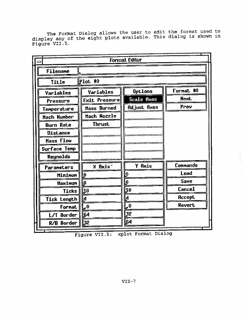
The Format Dialog allows the user to edit the format used todisplay any of the eight plots available This dialog is shown inFigure VII.5.
Format Editor
Title II_ #0
Variables
Presmure
Tenperature
Nach Number
Burn Rate Thrust
Distance
Nass Flo.
Sur£ace Temp
Reynolds
Hiniaue
Variables Options Fornat #0
.................°..............................
:::::::::::::::::::::::::::::::::::::::::::::::
Y Axis
Load
Haxiau. Save
Ticks LO LO Cancel
Tick Length _ _ Accept
Format ,0
L/T Border
R/B Border
Revert
Figure VII.5: xplot Format Dialog
VII-7

The format dialog will allow the user to edit the formats of
plots other than the active plot, and these plots need not beeither created or visible to edit their format. These formats can
be both loaded from and saved to external files for future use.
This dialog works in conjunction with the Data Attributes dialog
to modify the internal state of the formats of the plots.
Formats can be saved or loaded just like datasets. When the
program is begun, a default set of format values will be
installed for each available plot. The user can edit the format
to the style preferred, then save and recall these settings using
the Filename field. The Title field specifies the label that will
appear centered across the top of the plot.
There are two columns of toggle buttons labeled Variables.
The left column contains all of the variables in the current
dataset that are functions of both position and time. The
variables listed in the right column are functions of time alone.
Note that nothing will be displayed on the plot if the user
selects only time-dependent data from the Format dialog and
attempts to create a space plot. The organization of data in a
plot file is discussed in Section VI.
By selecting one of the toggle buttons in the Options
column, the user can determine which features to use on the
current plot. The first option, "Scale Data", forces the Y axis
to take on minimum and maximum values corresponding to the
minimum and maximum vales of the data displayed on the plot. The
second option, "Smooth Data", sets the minimum and maximum values
and the number of gridlines to even numbers that are more
appealing. None of the other six options are currently defined.
Values for both the x- and y-axes can be set using the text
fields at the bottom of the dialog. If the "Scale Data" option is
not active, then the minimum and maximum values of either axis
can be set manually. Note, however, that both minimum and maximum
must be set for each if any are to be set. The number of
gridlines and labels for either axis can be set in the same way.
The minimum number of gridlines is i, and the maximum is 20. The
borders affect the way the plot is sized and drawn. The text
fields in the x-axis area control the size of the left and right
borders, and the text fields in the y-axis area control the
bottom and top borders. All plot decorations appear outside the
main plot area, so the borders may have to be resized to give the
plot an appropriate appearance.
The Format field dictates the number of decimal points and
total field width that is used in displaying the axis labels.
These values should be specified in terms of standard C
formatting patterns as used with the standard input/output
VII-8

function sprintf This format is very similar to the syntax
used for REAL variables in FORTRAN FORMAT specifications. The
commands available in the Format Dialog are summarized in Table
VII.4.
Table VII.4: Format Dialog Commands
Comma nd Act ion,m
Prev
Next
Load
Save
Cancel
Accept
Revert
Switches to the previous or next format specification. Any of
the formats numbered [0-7] can be edited at anz time.
Loads or saves the particular format being displayed to or
from the f_lename currently in the Filename field. ..
Dismisses the Format dialog. Retains the current contents of
the dialog, but does not save those changes to the plot or toa file.
Changes the properties of the plot corresponding to the
current format to the values input.
Changes the values in the dialog to either those values last
saved or the default values. This function is essentially the
same as switching to either the previous or next format and
then switchingback.
The Data Attributes dialog allows the user to customize the
appearance of the data displayed in the main content area of a
plot. This dialog is shown in Figure VII.6.
VII-9

.t
Data Attributes Editor• w •
DaLa Colors Dashes ......... Colors
_ro..°,L_ L " i_iIT-.,.er._.re.3 , - .....I.
Hath Nu,be.r., _ , J - L
Bu;n" Rate _ I _,
.... O/stance _ _4.... ' ] "" ....
I ..- rlo. _ ]il. LI.'S.rr.oeTe.,,Ls,, ]LI R...olds 2,, E K_._tPress.re_ L kllass Burned _' _" _ ' '
• " .2
_Hach Nozzle _ _,,Z, _ ,,
i_ ,, i|
Figure VII.6:
L Dashes -
[,
L., L,
IJ
.I
Lp,,
IZ l
xplot DAta Attributes Dialog
The first column contains an index into the colors specified in
the colors files. The color of the label containing the
variable name will be changed to this color whenever the dialog
is updated. The number of dashes _ be specified in the second
column. The format for entries in this column is the number of
pixels that should be drawn "on" followed by the number of pixels
that should be drawn "off", For instance, 20 pixels on followed
by I0 pixels off would be entered as "20 10". There are no
commands associated with the Data Attributes dialog, since it
only reflects additional information about the format currently
selected with the Format dialog.
The File Edit dialog provides an editable text field in
which the user can load, view, make changes to, and save ASCII
text files. This dialog is shown in Figure VII.7.
Vll-10

Jut Data
=
Figure VII.7: xplot File Editor Dialog
The dialog is modeled after the xedit application included
in the standard distribution of the X Windows from MIT. This
rather simple dialog contains three action buttons, a single-line
text field for entering filenames, and a large text field for
displaying the contents of text files. This dialog is included to
provide the user a simple capability of editing text files from
within the application, without having to quit and restart the
interface program or edit field in another shell tool. The load
and save buttons read in or write out their contents based on the
filename specified in the single-line text field. The contentseither of the text buffer or the external text file will be
overwritten upon executing one of these commands. The commands
available in the File Edit dialog are summarized in Table VII.5.
VII-f1

Table VII.5: File Editor Dialog Commands
Command Actionl m . , • H,
Done Dismisses the dialog. Maintains the current state
of the text displayed, but does not save those
changes to a file.
Save Saves the current state of the text to the
filename given in the Filename text field.
Load Loads the contents of the filename specified in
the Filename field into the current text buffer.
Overwrites the contents of the text buffer with
the contents of the file specified in the Filename
field. If the file does not exist (i.e., if the
filename represents a new file), then that file is
opened (if possible) and the contents of the text
buffer are cleared.
The View Dataset dialog provides a simple read-only text
field area displaying the currently loaded dataset. This dialog
is shown in Figure VII.8.
_i S 25 4
_ressureTenperatureItach Nunber
i Burn Rat,eOlsLanceIlass FlouSurface TenpReynoldsFx.i.t, Pressureflass BurnedNach NozzleThrust
0.1GGGG72.G7 13.91
57.97 12.53113.28 12.45168.58 12.45
"Figure- VII. 8 :
Dataset:. Jsou_eNcaven_ .plot
332.26 0.0149 0.0000 0.0000 O,301.09 0.0168 0.0000 0.0000 O,299.09 0.0159 0.0000 0.0000 0,289.09 0.0158 0.0000 0.0000 O,
xplot View Dataset Dialog
This dialog is provided only to allow the user to easily
view the values as data in the plots created. This dialog
functions just like the File Edit dialog, except it always
contains the text of the current dataset, and the text in it can
VII-12

be neither edited nor saved. The dialog can be resized accordingto the width of data it displays. There are no commands
associated with the View Dataset dialog. It must be shown or
hidden from either the Dataset menu or the Window Manager dialog.
A simple command-line interface (or CLI) is provided for
those users more comfortable with the more conventional means of
entering commands. Note that each of the commands available
through the CLI corresponds to one of the commands available in
the graphical interface. A summary of the commands available is
given in Table VII.7. In Table VII.7, the notation $i refers to
the first argument, $2 to the second, etc.
VII-13

Table VII.7: Command-Line Interface Verbs
Command
active
color
data
Args
plot
decrement
(dec)
edit
execute
(exec)
format
hide
increment
(inc)
input
load
plane
plot
quit
data
color
file
plot
file
path
exec
format
plot
plot
path
save format
show
space
time
plot
plot
plot
Description
Changes the active plot to the one specified in $i.
Changes the color associated with the data specified in $I
to the color specified in $2. Equivalent to changing the
appropriate "color" field on the Line Format dia!o @.
Loads the file specified in $I as the current dataset.
Decrements the plot specified in $i. If no argument is
given, the active plot is decremented. Equivalent to
selecting ._Decrement" in the Plot Manaper dialog.
Loads the file specified in $i as the text to be edited in
the File Edit dialo_ and raises this dialog. If no file is
9iven& then the previous £11ename is used.
Executes the Caveny program from the path specified in $i
and the application name specified in $2. If neither
argument is given, the defaults are taken from the values
most recently specified in the Execute dialop.
Changes the format being edited in the Format dialog
to the value specified in $i.
Hides the plot specified in $i. Equivalent to selecting
"Hide" for the appropriate plot in the Plot Manager dial o 9.
Increments the plot specified in $i. If no argument is
given, the active plot is incremented. Equivalent to
selecting "Increment', in the Plot Mana@er dialo@.
Loads the file specified in $i as the input dataset to be
used in the Input File Editor dialog and raises this Dialog.
If no file is specified, then the dialog is raised with a
new input dataset.
Loads a dataset from the full pathname given in $I.. If no
argument is given, it attempts to re-load the dataset most
recently used with a "load" command from the "Dataset" menu.
Sets a time/space plane on the currently active plot to $I.
If the value specified in $i is less than one or more than
the time/space planes available, no action is taken.
Creates th_ plot specified in $I.
Terminates executlon of xplot.
saves the current format specified in $i.
Shows the plot specified in $i. Equivalent to selecting
"Show" for th_e appropriate plot in the Plot Manager dialog.
Toggles the plot specified in Sl to being a space plot. If
no argument is given, the active plot is toggled. Equivalent
to toggling the "Space plot/Time Plot" button on the Plot
Manager Dialog.
Toggles the plot specified in $i to being a time plot. If no
argument is given, the active plot is toggled. Equivalent to
toggling the "Space plot/Time Plot" button on the Plot
Manager Dialog.
VII-14

The xplot application has a number of external files that
must be present to run properly. In addition, a number of
additional files can be used to configure the application
according to the user's preferences, or to provide additional
support for interactions with other programs.
In each of the following example listings, a vertical bar
and all text following it should be interpreted as comments and
should not be inserted into the input files.
XPlot.clr. This file specifies the colors available to be
used in the line format dialog. The file is composed of a number
of lines containing a number and a valid color name as specified
in the XIIR4 color database Blank lines in the input file are
ignored. These number-color pairs allow the user to define thecolors that will be available for the various traces of data. An
example file excerpt is given as Table VII.8:
1 White
2 Black
18 Red
19 Green
20 Blue
Table VII.8:
II
Xplot.clr. File Format
Color #I = White (255, 255, 255)
Color #2 = Black ( 0, 0, 0)
Color #18= Red (255, 0, 0)
Color #19= Red ( 0, 255, 0)
Color #20= Red ( 0, 0, 255)
The XPlot.var file contains entries for all of the data to
be placed in a Caveny program input dataset generated by the
xplot program. Each variable entry in this file consists of a
number of parameters surrounded by a leading and a trailing
double-quote. The separate fields are terminated by a trailing
slash (/). The fields of a variable entry are (in order): the
variable list index, the FORTRAN name of the variable, A short
definition of the variable, its default value (in appropriate
units), and an optional long description. An example format of
the entries is given in Table VII.9.
Table Vll.9:T!
0/
NDELX /
Number of spacewise steps(dx)
along the propellant grain/2O/
Maximum value = 29
Format: Integer Units: None7J
XPlot.var File Format
Leading double-quoteVariable list index
FORTRAN variable name
Short variable description
. °°°
Default value
Long variable description
Trailing double-quote
VII-15

The application-defaults file. The resources specified inthe XPlot file located in the same directory with the xplotexecutable will be loaded in as fallback resources. Sinceuser-specified resources take precedence over fallback resourcesspecified by the application, resources set in either the user's.Xdefaults file or an XPlo_ file in the user's home account willoverride these settings.
Plot format files: Unlike the input files already described,
there can be any number of plot format files, and they can have
any name. The default format file, which is read upon program
start-up, is named XPlot.def. This file is a simple text file
enumerating the options selected in a plot format dialog. Each of
the fields stored in the dialog is reflected in the file, in the
same order as they appear in the dialog. Although there is no
reason why the user could not edit this file using either the
Input File dialog or a separate text processor, there is no
reason to do so. These files are read and created by the Plot
Format dialog directly. A sample listing for the XPlot.def file
is given as Table VII.10.
Table VII I0:
Plot #0
0 00 0 0 0 0 00 0 0 00 0 0 0
0 0 0 0 0 0 0 064 54 32 32
10.4 10.4i0 I0
Sample XPlot.def FilePlot title
Space data shownTime data shown
Options selectedBorder (L, T, R, B)Axis label formats
Number of axis gridlines/labels
The example plots shown in this section were all produced by
xplot with data generated by the Caveny program. All example
plots used the default values for format attributes from the
XPlot.clr and Xplot.def file_ _ The setup required for the plots
is described in the text following the plot. The data for these
plots was generated by the Caveny code from the sample input file
given as Appendix A.
Figures VII.9-VII.12 show the development of pressure in the
motor at four different times (30, 60, 90, and 120 milliseconds,
respectively). These plots trace the propagation of the initial
igniter motor pressure wave down the length of the grain.
Figures VII.II and VII.12 are shown to the same scale to
illustrate the effects of combustion on the chamber pressure. At
90 milliseconds, the grain has just begun to burn, and the spike
towards the aft end of the section results from the igniter mass
flow. At 120 milliseconds, much more of the grain has begun to
burn, and combustion gases from the head end have made their way
down the chamber.
VII-16

Pressure Plot
\
Figure VII.9: Pressure versus Location at Time=30 ms
.._ iressire PIOt li
1111 "'-4-11._I
Figure VII.10: Pressure versus Location at Time=60 ms
VII-17
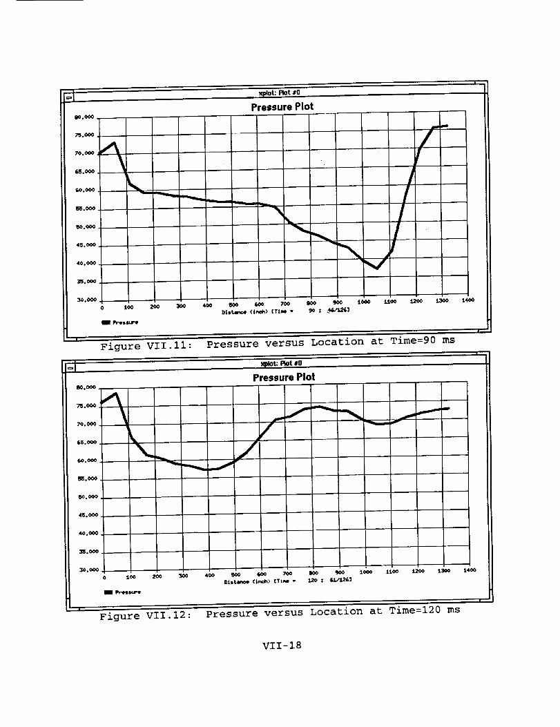
Pressure Plot
[1:.: --____ iII.:_i.... -__ J /
Figure VII,11: Pressure versus Location at Time=90 ms
H-' ' < C;?,:;,o, '11Iliii I I I I I il
._1 kl I /I L,."1I I 1II II
IIi"7l '1 III1,-IIIIIll/' i
Figure VII.12: Pressure versus Location at Time=120 ms
VII-!8

These four plots are typical of the default type produced by
xplot. All of the data are presented as a function of distance
along the motor geometry. Figures VII.9 - VII.12 represent four
time slices of the entire motor. Each plot contains a maximum of
30 points per curve, since this number is the maximum that the
Caveny program allows for axial stations. Pressure was the only
variable selected from the format dialog. The time was set using
the Increment and Decrement buttons on the Plot Manager dialog.
The scaling and number of gridlines were set manually. The number
of decimal places for the x-axis were left at their default value
of zero, but the y-axis labels were set to a 0.3 format.
Figures VII.13 and VII.14 show the data generated by the
Caveny program in a different fashion. These plots illustrate the
time history of a scalar quantity at two different axial
distances along the motor. In this particular example, the
chamber pressure is displayed as a function of time at the head
end and aft end stations. Each of these plots contains 126 data
points, since the Caveny input file was configured using its
print interval and total simulation time to generate this number.
This viewing option is set using the Space Plot/Time Plot toggle
button on the Plot Manager dialog. With this option, the user can
quickly switch back and forth in the manner chosen to view the
data. The station is selected using the Increment and Decrement
buttons on the same dialog. The scales, grids, and title were
each set manually.
VII-19

_I xplot:Plot #0|
LSO.O00
1.70.000
L60.0,00
L50.O00
L4G. O.O0
L30oO00
L.-_. 000
LLO.,O00
LOC,.O00
90.000
8,0.000
70.0,00
C_. 0¢,0
SO.,O00
40°000
30.000
20.000
t0.00¢,
Pressure Plot
r f4. _j
J
/
f
/
0 26 80 75 J.OO _ £60 L76 200 _ 260
Tim@ (mseo) [DLs% - 3 _: _L2 LMS]
m Pr, esm
Figure VII.13: Pressure versus Time at Distance=3 cm
1(.¢,.00¢
:LSO.OOO
t44:..00¢
i]K:,. 00¢
120.0,_
1i0.000
J.oo.ooo
90.0,00
80.000
7C,,0,00
(_,.00_
50,000
40.C,00
30,000
20.000
£0.000
_/ot: Mt #0
Pressure Plot
J
25 5O 75 100 12'3 LSO 175 2OO 225
Tl_ (tsec) [Dis% - 1330 : 25/ 2S]
am Pr'essuee
250
Figure VII.14: Pressure versus Time at Distance=1330 cm" I
VII-20

Figures VII.15 and VII.16 show that multiple traces of data
can be displayed on a single plot. In these two figures, the Mach
number and grain burn rate are shown as functions of distance attwo different times in the simulation (90 and 180 milliseconds).
Of interest in the first plot is the spike in Mach number and the
sharp drop-off in burn rate near the aft end of the motor. The
spike again corresponds to the igniter discharge, and the burn
rate reflects the fact that the aft end of the motor has not yet
begun to burn. By 180 milliseconds, both curves have flattened
out to more stable values all along the motor. In each plot, the
legend reflects the colors associated with the traces for the two
variables.
To configure these two plots, Mach number and burn rate were
the only variables selected using the Format dialog. To make the
traces print more distinctly, the colors and dashes for burn rate
were changed from their default values. Using the Format Lines
dialog, the burn rate color was set to black, and the dashes were
set to 20 on I0 off (by entering "20 10" in the variable's
appropriate field). In these two figures, the plots were manually
titled and automatically scaled.
.... -' |
...wr-
f
mm _mmB m mm m
xpk)_ _t to
Mach Number & Bum Rate Plot
f
I_m_ qmm
J
A"*k
.._ \
h
t00 200 300 44)0 500 _ 700 800 _OO 1000 11(_ 1200 1300 i4w_
_istar,_ (in_a) [Time = _0 | 4&/_26]
|
Figure VII. 15: Mach Number & Burn Rate versus Distance atTime=90 ms
VII-21

_t: Rot#0
Mach Number & Bum Rate Plot
Im ai m mlm maim --_ --
i ,, ,
aq mdm m lmm
i
i,_ _im maim m_
ttJ
500 600 700 80¢ 900 t000 J_iO0 i200 i300 1_00
Dis_ (inc_) [Time • £_ _ 9t,+126]
Figure VII.16: Mach Number & Burn Rate versus Distance at
Time=180 ms
!
Figures VII.17 and VII.18 are presented as examples of
variables that are functions only of time and not distance along
the grain. In these two figures, the Reynolds number at the exit
of the motor and the thrust generated by the motor are plotted.
The curve for the thrust produced is in accordance with the plot
of aft end pressure shown in Figure VII.14. The thrust is zero
until the igniter gases begin to be discharged at approximately
65 milliseconds. The Reynolds number at exit is a predominantly
linear function with the exception of the ignition spike from 60to i00 milliseconds. ......
To create plots of variables that are time-dependent only,
the Time Plot option must be selected from the Plot Manager
dialog. If this option is not chosen, no data will be drawn in
the plot frame. Note that the Increment and Decrement buttons in
this dialog do not function if only time-dependent variables are
selected. In all other aspects, these variables are configured
and displayed in exactly the same way as the other variables when
plotted as functions of time.
VII-22

xpIot: Plot #o -"-"-
4O000000
380O0O00
30000000
ZSOOOOOO
LSO0000O
LOOO00OO
SO00000
0
0
_J26
Reynolds Number Plot
mo 715 1oo £215 i6o
Time <reset) Cgist - L330 : 25/ ZSJ
mE Re_olds
J
i715 200 226 260
--! !
Figure VII.17: Reynolds Number at Exit versus Time
xplot: Riot #0
t5000¢
tO00_¢
]_0000
I00000
."50000
L5¢¢<)¢
LO0000
I_000
0
I Thr,,_t
A
2S SO _S
Thrust Plot
J
lo_ 12S 1_o
Time (.see) [])ist; • i]30 : 25/ 2'J3
f
i_5 200 22S 26O
' _ i
Figure VII.18: Motor Thrust versus Time
VII-23

APPENDIX A
Sample Caveny Program Input File
A-I

1234
56789101112131415161718192021222324252627282930313233343536373839404142434445464748495051525354
555657585960616263646566
6768
MM-I 17DEC77&NAME
TMAX = 0.002,TPRINT = 0.001,DELTAT = 0.00016,NDELX = 24,
TPI = 298.89,PAM = 0.84717,
UNIT = -2.0,TIGN = 2685.4,
TFREF = 3353.0,.W = 28.18, '.
GAMA = 1.136,AT = 2325.81,XP = 2.67,
XE = 1329.972,RUFSUR = 0.01,
FKPR = 0.0011,ROPR = 1.758,CPR = 0.3,
SIGP = 0.0009939,RREF = 1.054,PREF = 68.08,EBC = 0.0,
BREXP = 0.33,DE = 145.64,CM = 0.97844,
ALFAD = 12.31,GAMAN = 1.1348,
PISUBK = 0.0027,DELTTF = 0.00906,DFSDT = 0.01,
NIGTAB = 19,NAPDVX = 25,NDATA = 3,
TPRINT = 0.002,BF1 = 0.1, 0.1, 0.1, 27"1.0,CHC = 1.4, 1.3, 1.2, 1.1, 26"1.0,
DELTFF = 0.010, 0.007, 0.005, 27"1.0,DDHC = 0.94,
TPSCRI = 850.0,FCRIT = 0.1,
NBL = i0,NPUNCH = I,NBPTAB = 20
&END2
0.0000 0.00001.0000 1.0000
20.0000 0.00001.0000 1.0000
20.0000 0.00001.0000 1.0000
20.0000 0.00001.0000 1.0000
20.0000 0.00001.0000 1.0000
20.0000 0.00001.0000 1.0000
20.0000 0.00001.0000 1.0000
2
FLAME SPREAD CONTROL AT HEAD END ,DYNAMIC THRUST CHECKOUT
A-2

69707172737475767778798O818283
84858687888990919293949596979899100101102103104105106107108109110
117112113114115116117118119120121122123124125126127128129130131132133134135136137
0.00001.0000
20.00001.0000
20.00001.0000
20.00001.0000
20.00001.0000
2
0.00001.0000
20.00001.0000
20.00001.0000
20.00001.0000
20.00001.0000
20.00001.0000
20.00001.0000
20.00001.0000
0.0.020.0280.0440.0520.0640.O70.0880.180.240.2880.3440.3560.380.4240.460.5080.5560.566
2.67057.970
113.280168.580223.890279.190334.500389.800445.100500.410555.710611.020
0.00001.0000
0.00001.0000
0.00001.0000
0.00001.0000
0.00001.0000
0.0000
1.0000
0.00001.0000
0.00001.0000
0.00001.0000
0.00001.0000
0.00001.0000
0.00001.0000
0.00001.0000
1.18.1146.95406.05484.35514.35516.69510.06427 47392 42371 00348 43339 86313 75275 18253 38232 73219 50.02538.4402543.6202561.7002706 8702612 1002645 0002658 8502705 3202774 5302844 4202915 1903029 790
115411561144278181182182184186189191.195.
450490950930180310790380720060400130
1154.451156.491144.95278.93181.18182.31182.79184.38186.72189.06191.40195.13
31.
329.52
649.52
22439.
877.
2896.
59741.
20151.
20003.
2.21
1.5
1.5
A-3

138139140141142143144145146147148149150151152153
154155156157158159160161162163164
666 320721 630776 930832 230887 54O942 840998.150
1053.4501108.7601164.0601219.3601274.6701329.9720.6808
4.765168.08&NAME
TMAX =DELFAC
&END&NAME
TMAX =&END&NAME
TMAX =
2757.9302720.0902789.3002859.3802930.3303072.2803025.3103224.0303731.7004316.4304946.2005404.3505594.6700.10020.43831.054
0.01,z 1.3
0.30
0.40,TPRI_ = 0.005
&END
186.160184.880187.220189.560191.890196.490194.980201.280216.550232.900249.310260.600265.150
186.16184.88187.22189.56191 89196 49194 98201 28216232249260265
942.
55931 1293.2615
3653.
15349.
19531.
77964.
1.5
9.1
A-4

APPENDIX B
Caveny Program Makefile
B-I

7
8
9
I0
11
12
13
14
15
16
17
18
19
2O
21
22
23
24
25
26
27
28
29
30
31
32
33
34
35
36
37
38
39
40
41
42
43
44
45
46
47
48
49
5O
# File: makefile
# This file contains all dependencies necessary to make the caveny code
F77 = f77
FFLAGS= -g
OBJECTS = \
ans.ok
brcal.ok
fccal.o\
fct.ok
fct2.o\
lilt.o\
hccal.o\
inhomo.o\
iterpl.ok
lagin2.o\
ibc.o\
migdot.ok
pnch.ok
prepc.o\
prepp.o\
rbc.o\
redpun.o\
runge.ok
sdata.ok
sdatac.o\
slotk.ok
solutc,o\
solutp.o\
srnbug.o\
thrusl.ok
timest.ok
trid.o\
decomp.ok
solv.o\
gsolv.ok
asolv.ok
vsolv.ok
repl2.o\
repll,o\
sing,ok
tscal.ok
main.o
caveny: $(OBJECTS)
$(F77) $(FFLAGS) -o caveny $(OBJECTS)
B-2

APPENDIX C
xplot Source Program
C-I

12345678910111213141516171819202122232425262728293031323334353637
38394O41424344454647484950515253545556575859606162636465666768
/*
xpCommands.c................................. . .....................................
*!
#include "xpIncs.h"#include "xpDefs.h"
#include "xpwidgets.h"#include "xpgeneral.h',#include "xpmenus.h"#include "xpformats.h"#include "xpplots.h"
#define cSpace 32#define cTab 9
/* $1: Global variables */
char cli[64]=('');char cliString[16][64]={ ................................ ), a i , t t e # p # o ; f p ; ;
int cliIndex=0,cliNum=0;
/* $2: Local variables - (none) */
char con_ndString[16] [32], *co_nandStack[16];char inputString[64];
/* $3: Global functions */
void Listcallback();void SaveCommuknd();void RecallCommand();void Echo();
/* $4: Local functions */
void Push();void BreakdownString();void DoParse();
/* $5: Implementation == = z = =
void ListCallback(w, client data,call_data)Widget w; XtPointer client_data, call_data;
{XawListReturnStruct *r _ (XawListReturnStruct*) call_data;
char s[64];
strcpy(s, (*r).string);XtVaSetValues(cliText,XtNstrlng,s,NULL);XawTextSetInsertionPoint(cliText,strlen(s));
)
void SaveCommand (w, event, params, numParams)Widget w; XEvent *event; String *params; Cardinal *numParams;
{XawTextPosition n;char s[64], *ss;int hum;
X£VaGetValues(cliText,XtNstring,&ss,NULL);n=strlen(ss);if (n>0) {
if (n>63) n=63;strncpy(s,ss,n);S [n] =' \0' ;
C-2

697071727374
75767778798O8182838485868788899O919293949596979899i00101102103104105106107108109110111112113114115116117118119120121122123124125126127128129130131132133134135136137
Push(st;cliNum++;cliIndex=0;XtVaSetValues(cliText,
XtNstring,'',XtNinsertPosition,strlen(''),NULL);printf('>cli: %3d %s\n',cliNum, s);
)strcpy(inputString, s);BreakdownString(inputString,commandString,&num);DoParse(num, commandString);
void RecallCommand(w,event,params,numParams)Widget w; XEvent *event; String *params; Cardinal
(
)
void Echo(s)
String s;{
int sLength=strlen(s),code;XawTextBlock text;
text.firstPos=0; text.length=sLength;
code = XawTextReplace(logText,startPos,endPos,&text);startPos = startPos+sLength;endPos = startPos;XawTextSetInsertionPoint(logText,startPos);
)
void Push(st
String s;(
int i;
for(i=(NUMcliString-l);i>l;i--)strcpy(cliString[i],cliString[i-l]);
strcpy{cliString[l_,s);strcpy(cliString[0],'');for (i=0;i<NUMcliString;i++)
commandStack[NUMcliString-i-l]=cliString[i);XawListChange(commList,commandStack,15,0,False);
)
void BreakdownString(old,new, count)char old[]; char new[][32]; int *count;
(int i=0,m=0,n=0;
while (oid[i]!='\0') {
while ((old[i]=icSpace) Ii(old[i]==cTab))i+÷;
while
*numParams ;
if(*numParams>0)
if(params[0][0]=='l') {if((cliIndex<cliNum)&&(clilndex<15)) (
cliIndex++;XtVaSetValues(cliText,XtNstring,cliString[cliIndex],NULL);XawTextSetInsertionPoint(cliText,strlen(cliString[cliIndex]));
))if (params [0] [0]=='2') {
if(cliIndex>0) (cliIndex--;XtVaSetValues(cliText,XtNstring,cliString[cliIndex],NULL);XawTextSetInsertionPoint(cliText,strlen(cliString[cliIndex]));
))
text.ptr=s; text.format=FMTSBIT;
((old[i]!=cSpace)&&(old[i]!=cTab)&&(old[i]!='k0')&&(n<32)) (
C-3

138139140141142143144145146147148149150151152153154155156157158159160161162163164165166167
168169170171172173174175176177178179180181182183184185186187188189190191192193194195196
197198199200201202203204205206
new[m][n] = old[i];i++;
n++ ;)new[m] [n]='\0';
m++;n=0;
)*count=m;
)
void DoParse(argc,argv)int argc; char argv[][32];
(int l,m,n;
if (argc>0) (if (strcmp(argv[0],'quit')==0) {
exit(0);)else if (strcmp(argv[0],'change')==0) {
printf('(<change> unimplemented}\n');)else if (strcmp(argv[0],'decrement')==0) (
printf('{<dec[rement]> unimplemented)\n');)else if (strcmp(argv[0],'edit')==0) (
printf('{<edit> unimplemented}\n');)else if (strcmp(argv[0],'execute')==0) {
printf('(<exec[ute]> unimplemented)in');)else if (strcmp(argv[0],'hide')==0) (
if (argc>2) {if (strcmp(argv[l],'plot')==0) {
n=atoi(argv[2]);if ((n>=0)&&(n<=MAXPLOTS)&&{plotExists[n]))
ShowHide2(dummy,wPlot0+n,False,0);)
)
)else if (strcmp(argv[0],'increment')==0) {
printf('{<inc[rement]> unimplemented}\n');)else if (strcmp(argv[0],'kill')==0) {
if (argc>l) {if(strcmp(argv[l],'plot')==0) (
if (argc>2) {n=atoi(argv[2]);if ((n>=0)&&(n<MAXPLOTS)&&(plotExists[n]))
KillPlot(n);)
))
))else if (strcmp(argv[0],'load')==0) {
if (argc>l) {if (strcmp(argv[l],'data')==0) {
LoadData (dsName) ;)
))else if (strcmp(ar_v[0],'make')==0) (
if (argc>2) (n=atoi(argv[2]);if((n>=0)&&(n<MAXPLOTS)&&(!plotExists[n])) {
MakePlot(n);
C-4

207
2O8
209
210
211
212
213
214
215
216
217
21B
219
220
221
222
223
224
225
226
227
228
229
230
231
232
233
234
235
236
237
238
239
240
241
242
243
244
245
246
247
248
1
2
3
4
56
7
B
9
10
11
12
13
14
15
16
17
1819
20
21
22
23
24
25
26
27
]]
/*
)]else if (strcmp(argv[0],'print')==0) {
printf('{<print> unimplemented)\n');
)else if (strcmp(argv[0],'save°)==0) {
printf('{<save> unimplemented)\n');
)else if (strcmp(argv[0],'set')==0) {
if (argc>l) (
if (strcmp(argv[l],'data')==0) [
if (argc>2)
strcpy(dsName,argv[2]);
SetStatusLabel{);
}else SelectString(1);
)if (strcmp(argv[l],'format')==0) {
if (argc>2) [
strcpy(pfName,argv[2]);
SetStatusLabel();
)else SelectString(2);
})
)else if (strcmp(argv[0],'show')==0) {
if (argc>2) {
if (strcmp(argv[l],'plot')==0) [
n=atoi(argv[2]);
if ((n>=0)&&(n<=7)&&(plotExists[n]))
ShowHide2(dummy,wPlot0+n,True,0);
))
}else if (strcmp(argv[0],°view')==0) {
printf('{<view> unimplemented}\n');
)else printf(°{unrecognized command [%s] [%d]...)kn',argv[0],argc-l);
xpData, c
*/
#include "xplncs.h"
#include "xpDefs.h"
#include "xpplots.h"
#include "xpwidgets.h"
/* $i: Global variables */
Boolean dataLoaded=False;
char columnNames[2*MAXCOLS][24];
int numPlanes,numCols,numRows,numTimeDep;
int currentPlane[MAXPLOTS]={O,O.O,O,O,O,O,O);
int currentRow[MAXPLOTS]={0,0.0,0,0,0,0,0);
float x[MAXROWS];
float z[MAXPLANES];
float plotData[MAXPLOTS][2*MAXCOLS][MAXPLANES];
float dMin[MAXPLOTS][2*MAXCOLS];
float clMax[MAXPLOTS][2*MAXCOLS];
C-5

28
29
30
31
32
33
34
35
36
37
38
39
40
41
42
43
44
45
46
47
48
49
50
51
52
53
54
55
56
57
58
59
60
61
62
63
64
65
66
67
686970
71
72
73
74
75
76
77
78
79
B0
%1
82
83
B4
85
86
87
88
89
90
91
92
93
94
9596
float
float
float
/° $2:
float
/* S3:
xMin,xMax,xRange;
zMin,zMax, zRarlge;
yMin[MAXPLOTS],yMax[MAXPLOTS],yRange[MAXPLOTS];
Local variables */
d[MAXPLANES][MAXCOLS+I][MAXROWS];
Global functions */
void LoadData();
void PrintData();
void CopyData();
/* $4: Local functions */
void StatInd();
void StatData();
void PrintPiotData();
/* $5: Implementation .............. ================================= */
void LoadData(infile)
char *infile;
(FILE *fi;
int i,j.k,n=0;
float dumray;
char s[64];
printf('>Now loading dataset from file: <%s>\n',infile);
fi = fopen(infile,'r');
if(fi!=NULL) {
strcpy(s.'Dataset: ");
strcat(s,infile);
XtVaSetValues(dataShell,XtNtitle,s.NULL);
XtVaSetValues(dataText,XtNstring, infile,NULL);
for (i=0;i<8;i++)
XtVaSetValues(PMitem[l][i],XtNsensitive,True,NULL);
dataLoaded=True;
fscanf(fi,'%d%d%d%d\n'.&numCols,&numRows,&numTimeDep);
for (k=0;k<numCols;k++) (
fgets(columnNames[k],25, fi};
for (i=0;i<strlen(columnNames[k]);i++)
if (columnNames[k][i]=='\n') columnNames[k][i]='\0';.
XtVaSetValues(FEItem[l] [k].XtNlabel.columnNames[k],
XtNsensitive.True,NULL);
XtVaSetValues(CFItem[O][k],XtNlabel.columnNames[k],
XtNsensitive,True,NULL);
XtVaSetValues(DAItem[0] [k],XtNlabel,columnNames[k].NULL);
}for (k=0;k<numTimeDep;k+÷) [
fgets(columnNames[MAXCOLS+k].25,fi);
for (i=O;i<strlen(columnNames[MAXCOLS+k]);i÷+)
if (columnNames[MAXCOLS+k][i]=='kn')
columnNames[MAXCOLS+k][i]='\0';
XtVaSetValues(FEItem[2][k],XtNlabel,columnNames[MAXCOLS+k],
XtNsensitive. True,NULL);
XtVaSetValues(CFItem[0][MAXCOLS+k],XtNlabel,coltnTunNames[MAXCOLS+k].
XtNsensitive,True. NULL);
XtVaSetValues(DAItem[0][8+k],XtNlabel.columnNames[MAXCOLS+k],NULL);
}if ((numRows>0) && (numCols>0)) (
k=0;
do (
n=fscanf(fi,'%e',&z[k]);
if (n!=EOF) {
for(i=O;i<numRows;i++) (
if(k==0)
C-6

97
98
99
i00
i01
102
103
104
105
106
107
108
109
110
iii
112
113
114
115
116
117
118
119
120
121
122
123
124
125
126
127
128
129
130
131
132
133
134
135
136
137
138
139
140
141
142
143
144
145
146
147
148
149
150
151
152
153
154
155
156
157
158
159
160
161
162
163
164
165
fscanf(fi,'%e',&x[i]);
else
fscanf(fi,'%e',&dummy);
for(j=0;j<numCols;j++)
fscanf(fi,'%e',&d[k][jl [i_);
)
for (i=0;i<numTimeDep;i++)
fscanf(fi,°%e',&d[k](MAXCOLS][i]);
)k++;
} while ( (n!=EOF)&&(k<(MAXPLANES-I)));
)numPlanes=k-l;
fclose(fi);
StatInd();
)else printf('Unable to load dataset (does not exist)\n');
void PrintData(outfile)
char *outfile;
{FILE *fo;
int i,j,k;
printf('>Now printing dataset to file: <%s>kn',outfile);
fo = fopen(outfile,'w');
fprintf(fo,'%4d %4d %4dkn',numPlanes,numCols,numRows);
if ((numRows>0) && (numCols>0) && (numPlanes>0))
for(k=0;k<numPlanes;k++) (
fprlntf(fo,'%12.6f\n',z[k]);
for(i=0;i<numRows;i++) (
fprintf(fo,'%12.6f',x[i]);
for(j=0;j<numCols;j++)
fprintf(fo,'%12.6f',d[k][j][i]);
fprintf(fo,'\n');
})
fclose(fo);
void CopyData(plotNum)
int plotNum;
(int i,j;
if (planar[plotNum])
for(j=0;j<numCols;j++)
for(i=0;i<numRows;i++)
plotData[plotNum][j][i]=d[currentPlane[plotNum]] [j][i];
else {
for(j=0;j<numCols;j++)
for(i=0;i<numplanes;i++)
plotData[plotNum][j] [i]=d[i][j] [currentRow[plotNum]];
for(j=0;j<numTimeDep;J++)
for(i=0;i<numPlanes;i++)
plotData[plotNum][MAXCOLS+j][i]=d[i] [MAXCOLS][j];
))
void StatData(p)
int p;
(int i,j0m,n,test;
float Max,Min;
int count;
count = (planar[p] ? numRows : numPlanes);
test = (planar[p] ? MAXCOLS : 2*MAXCOLS);
C-7

166167168169170171172173174175176177178
179180
181182183184
185186187188189190
1911921931941951961971981992002012022032042052O6207208209
210211212213214215216217218219220221222223224225226227228229230231232233234
for (j=0; j<test ;j++)if (useCol[p] [j]) {
Min= i000000;Max=-1000000;for (i=0 ;i<count; i++) {
if(plotData[p] [j] [i]<Min)if (plotData[p] [j] [i] >Max)
)dMin [p] [j]=Min;dMax [p] [j ]=Max;
}
Min=plotData[p] [j] [i] ;Max=plotData [p] [j] [i];
Min= i000000;Max=-1000000;
for(j=0;j<test;j++)if (useCol[p] [j]) (
if(dMin[p] [j]<Min) Min=dMin[p] [j] ;if(dMax[p] [j]>Max) Max=dMax[p] [j] ;
}
yMin[p]=Min;yMax[p]=Max;yRa_ge[p]=yMax[p]-yMin[p];if (yRange[p]<=0.001) (
yRange[p]=l.0;yMax[p]=yMin[p]+l.0;
)
void StatInd (){
int i;xMin= i000000;xMax=-1000000;for(i=0;i<numRows;i÷+) {
if(x[i]<xMin) xMin=x[i];if(x[i]>xMax) xMax=x[i];
)xRange=xMax-xMin;zMin= 1000000;zMax=-1000000;for(i=0;i<numPlanes;i++) [
if(z[i]<zMin) zMin=z[i];if(z[i]>zMax) zMax=z[i];
)zRange=zMax-zMin;
void PrintPlotData(p)int p;
(int i,j,k;
printf('>Now printing plotset(%d)...\n',p);printf('%4d %4d %4d\n',currentPlane[p],numCols,currentRow[p]);if (planar[p]) {
if ((numRows>0) && (numCols>0))
printf('%10.4fkn',z[currentPlane[p]]);for(i=0;i<numRows;i÷+) [
printf('%10.4f',x[i]);for(j=0;j<numCols;j++)
printf('%10.4f',plotData[p][j][i]);printf('\n');
}
printf('xMin: %10.4fkn',xMin};printf('xMax: %10.4f\n',xMax);printf('xRange: %10.4fkn',xRange);
)else {
C-8

235
236
237
238
239
240
241
242
243
244
245
246
247
248
249
25O
251
1
2
3
4
5
6
7
8
9
I0
ii
12
13
14
15
16
17
18
19
2O
21
22
23
24
25
26
27
28
29
3O
31
32
33
34
35
36
37
38
39
4O
41
42
43
44
45
46
47
48
49
50
51
52
if ((numPlanes>0) && (numCols>0))
printf('%10.4f\n',x[currentRow[p]]);
for(i=0;i<numPlanes;i÷+) (
printf('%10.4f',z[i]);
for(j=0;j<numCols;j÷+)
printf('%10.4f',plotData[p] [j] [i]);
printf('\n');
)
printf('zMin: %10.4f\n',zMin);
printf('zMax: %10.4fkn',zMax);
printf('zRange: %10.4f\n',zRange);
)
printf('yMin: %10.4fkn',yMin[p]);
printf('yMax: %10.4fkn',yMax[p]);
printf('yRange: %10.4f\n',yRange[p]);
)
xpFormats.c
*/
#include °xpIncs.h"
#include "xpDefs.h*
#include "xpgeneral.h"
#include "xpwidgets.h"
#include "xpmenus.h"
#include "xpdata.h"
#include "xpplots.h"
#define feLoad 1
#define feSave 2
#define feCancel 3
#define feAccept 4
#define feRevert 5
/* $i: Global variables */
PlotFormat f[MAXPLOTS];
int activeFormat=0;
/* $2: Local variables - (none) */
/* $3: Global functions */
void InitFormat();
void SetFEValues();
void GetFEValues();
void RecalcFormat();
void FEToggleCallback();
void FECommandCallback();
void SetFEValues();
void GetFEValues();
/* $4: Local functions - (none) */
/*
void PrintFormat () ;
*/
/* $5: Implementation =============================================== */
void InitFormat(p)
int p;
{int i,j;
C-9

53
54
55
56
57
58
59
60
61
62
63
64
65
66
67
68
69
70
71
72
73
74
75
76
77
78
79
80
81
82
83
84
85
86
87
88
89
90
91
92
93
94
95
96
97
9899
lO0lol102
103
104
105
106
107
108
109
110
111
112
113
114
115
116
117
118
119
120
121
sprintf(f[p].title,'Plot #%d',p);
for (i=0;i<8;i++) (
f[p].color[i]=i;
f[p].color[MAXCOLS+i]=MAXCOLS+i;
f[p].numDashes[i]=0;
for (j=0;j<8;j++)
f[p].dashes[i][j]=0;
f[p].opt[i]=False;
)
f[pl.borderL=64; f[p].borderR=32; f[p].borderT=32; f[p].borderB=64;
f[p].xNum=10; f[p].yNum=10;
f[p].xMin=f[p).xMax=0; f[p].yMin=f[p).yMax=0;
strcpy(f[p].xFormat,'.0"); strcpy(f[p]..yFormat,'.0") ;
f[p].opt[aScaleAxes]=True; f[p].opt[asmoothNum]=False;
f[p].xTick=4; f[p].yTick=4;
f[p].width=640; f[p].height=480;
f[p].xInc=(f[p].width -f[p].borderL-f[p].borderR)/f[p].xNum;
f[p].yInc=(f[p].height-f[p].borderT-f[p].borderB)/f[p].yNum;
f[p].nGrid=f[p].xNum+f[p].yNum+2;
f[p].xLength=f[p].xNum*f[p].xInc;
f[p].yLength=f[p].yNum*f[p].yInc;
void SetFEValues(p)
int p;
(char s[16] [32],t[16];
int i,j;
strcpy(s[0],f[p].title);
XtVaSetValues(FEItem[FEBTitle][O],XtNstring, s[O],NULL);
for (I=0;i<(2*MAXCOLS);i++) {
sprintf(s[i],'%d',f[p].color[i]);
XtVaSetValues(DAItem[l] [i],XtNstring,s[i],NULL);
XtVaSetValues(DAItem[0][i],
XtNbackground, lineColor[f[p].color[i]],
XtNforeground, rColor[Black].pixel,NULL);
)
for (i=0;i<(2*MAXCOLS);i++) (
strcpy(s[i],'');
for (j=0;j<f[p].numDashes[i];j++) (
sprintf(t,'%d ", (int) f[p].dashes[i][j]);
strcat(s[i],t);
)XtVaSetValues(DAItem[2] [i],XtNstring,s[i],NULL);
)
sprintf(t,'%%%sf',f[p].xFormat);
sprintf(s[0],t,f[p].xMin);
sprintf(s[l],t,f[p].xMax);
sprintf(s[2],'%d',f[p].xNum);
sprintf(s[3],'%d',f[p].xTick);
strcpy(s[4],f[p].xFormat);
sprintf(s[5],'%d',f[p].borderL);
sprintf(s[6],'%d',f[p].borderR);
for (i=0;i<7;i÷+}
XtVaSetValues(FEItem[FEBX][i],XtNstring,s[i],NULL);
sprintf(t,'%%%sf',f[p].yFormat);
sprintf(s[0],t,f[p].yMin);
sprintf(s[l],t,f[p].yMax);
sprintf(s[2],'%d',f[p].yNum);
sprintf(s[3],'%d',f[p].yTick);
strcpy(s[4],f[p].yFormat);
sprintf(s[5],'%d',f[p].borderT);
sprintf(s[6],'%d',f[p].borderB);
C-10

122
123
124
125
126
127
128
129
130
131
132
133
134
135
136
137
138
139
140
141
142
143
144
145
146
147
148
149
150
151
152
153
154
155
156
157
158
159
160
161
162
163
164
165
166
167
168
168
170
171
172
173
174
175
176
177
178
179
180
181
182
183
184
185
186
187
188
189
190
for (i=0;i<7;i++)
XtVaSetValues(FEItem[FEBY][i],XtNstring, s[i],NULL);
for(i=0;i<MAXCOLS;i++)
if (i_numCols)
XtVaSetValues(FEItem[FEBVars] [i],XtNsensitive,True,NULL);
else
XtVaSetValues(FEItem[FEBVars][i],XtNsensitive,False,NULL);
for(i=0;i<MAXCOLS;i++)
if (i<numTimeDep)
XtVaSetValues(FEItem[2] [i],XtNsensitive,True,NULL);
else
XtVaSetValues(FEItem[2] [i],XtNsensitive,False,NULL);
for(i=0;i<numCols_i++)
XtVaSetValues(FEItem[FEBVars] [i],XtNstate,useCol[p][i],NULL);
for(i=0;i<numTimeDep;i++)
XtVaSetValues(FEItem[2][i],XtNstate,useCol[p][MAXCOLS+i],NULL);
for(i=0;i<8;i++)
XtVaSetValues(FEItem[FEBOpts] [i],XtNstate,f[p].opt[i],NULL);
void GetFEValues(p)
int p;
{String t;
char s[16][16];
int i,j,count,u[8];
XtVaGetValues(FEItem[0][0],XtNstring,&t,NULL);
strcpy(f[p].title,t);
for (i=0;i<(2*MAXCOLS);i++) {
XtVaGetValues(DAItem[l][i],XtNstring,&t,NULL);
strcpy(s[i],t);
j = atoi(s[i]);
f[p].color[i] = ((j>=0)&&(j<=31) ? j : i);
]
for (i=0;i<(2*MAXCOLS);i++) {
XtVaGetValues(DAItem[2] [i],XtNstring,&t,NULL);
strcpy(s[i],t);
count=sscanf(s[i],'%d %d %d %d %d %d %d %d',
&u[0],&u[l],&u[2],&u[3],&u[0],&u[l],&u[2],&u[3]);
f[p].numDashes[i]=count;
for (j=0;j<8;j+÷)
f[p].dashes[i] [j]=(char) u[j];
)
for (i=0;i<7;i++) {
XtVaGetValues(FEItem[FEBX] [i],XtNstring,&t,NULL);
strcpy(s[i],t);
)f[p].xMin=atoi(s[0]);
f[p].xMax=atoi(s[l]);
f[p].xNum=atoi(s[2]);
f[p].xTick=atoi(s[3]);
strncpy(f[p].xFormat,s[4],15);
f[p].borderL=atoi(s[5]);
f[p].borderR=atoi(s[6]);
for (i=0;i<7;i++) [
XtVaGetValues(FEItem[FEBY][i],XtNstring,&t,NULL);
strcpy(s[i],t);
)
f[p].yMin=atoi(s[0]);
f[p].yMax=atoi(s[l])_
f[p].yNum=atoi(s[2]);
f[p].yTick=atoi(s[3]);
strncpy(f[p].yFormat,s[4],15);
C-II
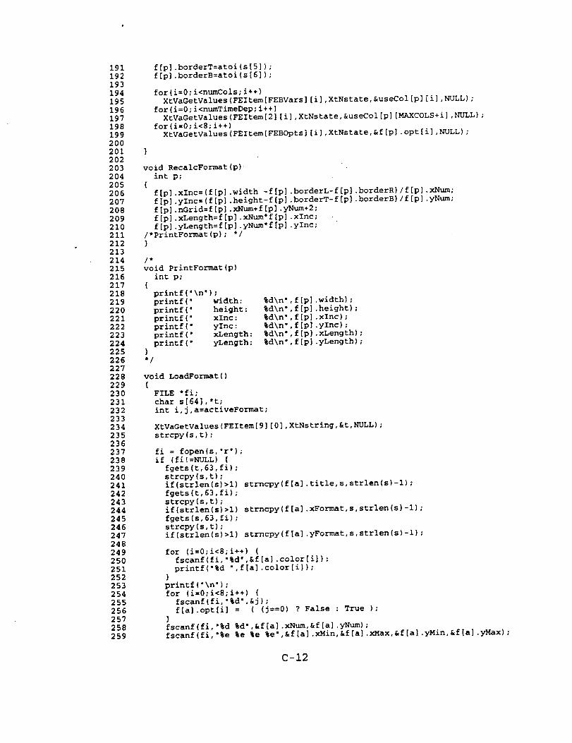
191
192
193
194
195
196
197
198
199
2OO
201
202
203
204
205
206
207
208
209
210
211
212
213
214
215
216
217
218
219
220
221
222
223
224
225
226
227
228
229
230
231
232
233
234
235
236
237
238
239
240
241
242
243
244
245
246
247
248
249
250
251
252
253
254
255
256
257
258
259
f[p].borderT=atoi(s[5]);
f[p].borderB=atoi(s[6]);
for(i=0;i<numCols;i+÷)
XtVaGetValues(FEItem[FEBVars] [i],XtNstate,&useCol[p] [i],NULL);
for(i=0;i<numTimeDep;i++)
XtVaGetValues(FEItem[2] [i],XtNstate,&useCol[p] [MAXCOLS+i],NULL);
for(i=0;i<8;i++)
XtVaGetValues(FEItem[FEBOpts] [i],XtNstate,&f[P]-opt[i],NULL) ;
void RecalcFormat(p)
int p;
(f[p].xInc=(f[p].width -f[p].borderL-f[p].borderR)/f[p].xNum;
f[p].ylnc=(f[p].height-f[p].borderT-f[p].borderB)/f[P]-yNum;
f[p].nGrid=f[p].xNum+f[p].yNum+2;
f[p].xLength=f[p].xNum*f[p].xInc;
f[p].yLength=f[p].yNum*f[p].yInc;
/*PrintFormat(p); */
)
void PrintFormat(p)
int p;
{printf('\n');
printf(" width:
printf(" height:
printf(" xInc:
printf(" yInc:
printf(" xLength:
printf(" yLength:
)*/
%d\n',f[p].width);
%d\n',f[p].height);
%d\n',f[p].xInc);
%dkn',f[p].yInc);
%d\n',f[p].xLength);
%d\n',f[p].yLength);
void LoadFormat()
(FILE *fi;
char s[64],*t;
int i,j,a=activeFormat;
XtVaGetValues(FEItem[9] [0],XtNstring,&t,NULL);
strcpy(s,t);
fi = fopen(s,'r');
if (fi!=NULL) (
fgets(t,63,fi);
strcpy(s,t);
if(strlen(s)>l)
fgets(t,63,fi);
strcpy(s,t);
if(strlen(s)>l)
fgets(s,63,fi);
strcpy(s,t);
if(strlen(s)>l)
strncpy(f[a].title,s,strlen(s)-l);
strncpy(f[a].xFormat,s,strlen(s)-l);
strncpy(f[a].yFormat,s,strlen(s)-l);
for (i=0;i<8;i++) (
fscanf(fi,'%d',&f[a].color[i]);
printf(o%d ",f[a].color[i]);
)
printf('\n');
for (i=0;i<8;i++) {
fscanf(fi,'%d',&j);
f[a].opt[i] = ( (j==0) ? False : True );
)
fscanf(fi,'%d %d.,&f[a].xNum,&f[a].yNum);
fscanf(fi,'%e %e %e %e.,&f[a].xMin,&f[a].xMax,&f[a].yMin,&f[a].yMax);
C-12

260
261
262
263
264
265
266
267
268
269
270
271
272
273
274
275
276
277
278
279
280
281
282
283
284
285
286
287
288
289
290
291
292
293
294
295
296
297
298
299
300
301
302
303
304
305
306
307
308
309
310
311
312
313
314
315
316
317
318
319
320
321
322
323
324
325
326
327
328
fscanf(fi,'%d %d',&f[a].xTick,&f[a].yTick);
fscanf(fi,'%d %d %d %d',
&f[a].borderL,&f[a].borderR,&f[a].borderT,&f[a].borderB);
fclose(fi);
SetFEValues{a);
void SaveFormat {)
(FILE * fo;
char s[64],*t;
int i,a=activeFormat ;
XtVaGetValues (FEItem[9] [0] ,XtNstring, &t, NULL) ;
strcpy(s,t) ;
if (s[0]!=NULL) {
fo = fopen(s,'w');
fprintf(fo,'%s\n'0f[a].title);
fprintf(fo,'%skn%skn',f[a].xFormat,f[a].yFormat);
for (i=0;i<8;i++)
fprintf(fo°'%d ",f[a].color[i]);
fprintf(fo,'\n');
for (i=0;i<8;i++)
fprintf(fo,'%d
fprintf(fo,'\n');
°,f[a].opt[i]);
fprintf(fo,'%d %d\n',f[a].xNum, f[a].yNum);
fprintf(fo,'%f %f %f %fkn',f[a].xMin, f[a].xMax, f[a].yMin, f[a].yMax);
fprintf(fo,'%d %d\n',f[a].xTick, f[a].yTick};
fprintf(fo,'%d %d %d %d\n',
f[a].borderL, f[a].borderR, f[a].borderT, f[a].borderB);
fclose(fo);
}
)
void FEPageCallback(w, client data,call_data)
Widget w; XtPointer client_data,call data;
(int i = (int) client_data;
char s[64];
switch (i) (
case 0:
if (activeFormat<(MAXPLOTS-l)) (
activeFormat++;
SetFEValues(activeFormat);
sprintf(s,'Format #%d',activeFormat);
XtVaSetValues(FETop[FEBFage],XtNlabel,s,NULL);
)break;
Case i: _ _= _ :_
if (activeFormat>0) (
activeFormat--;
SetFEValues|activeFormat);
sprintf(s,'Format #%d',activeFormat);
XtVaSetValues(FETop[FEBPage],XtNlabel,s,NULL);
}break;
)
void FECommandCallback(w,client_data,call_data)
Widget w; XtPointer client_data,call_data;
{
C-13

329
330
331
332
333
334
335
336
337
338
339
340
341
342
343
344
345
346
347
348
349
350
351
352
353
354
355
356
357
358
1
2
3
4
5
6
7
8
9
10
11
12
13
14
15
16
17
18
19
20
21
22
23
24
25
26
27
28
29
30
31
32
33
34
35
36
37
38
39
int i = (int) client_data;
switch (i) (
case feLoad:
LoadFormat();
break;
case feSave:
SaveFormat() ;
break;
case feCancel:
ShowHide2(dummy,wFormat,True,0);
SetFEValues(activeFormat);
break;
case feAccept:
GetFEValues(activeFormat);
if (plotExists[activeFormat]) {
RecalcFormat(activeFormat);
StatData(activeFormat);
SetupGrid(activeFormat);
SetupAxisLabels(activeFormat);
SetupPoints(activeFormat);
RedrawPlot2(activeFormat);
}
break;
case feRevert:
SetFEValues(activePlot);
break;
)
)
/*
xpGeneral.c..................... . ........... J--.. .... . ...... -- ......................
*/
#include "xpIncs.h"
#include "xpDefs.h"
#include "xpwidgets.h"
#include "xpcommands.h"
#include "xpdata.h"
#include "xpplots.h"
/* $I: Global variables */
Screen *screen;
Display *display;
Boolean windowUp[48];
GC gc[MAXGCS];
XColor exact,color[16],rColor[16];
Font f6xl0,f6xl2,f6xl3,fHelvl8b;
XFontStruct *fs6xl0,*fs6xl2,*fs6xl3,*fsHelvlSb;
XawTextPosition startPos=0,endPos=0;
char inName[64]={''},dsName[64]=(''},pfName[64]={''},plName[4]=('');
/* $2: Local variables - (none)
/* $3: Global functions */
void LoadFonts();
void LoadColors();
void InitData();
void ProcessKey();
void Idle();
*!
/* $4: Local functions - (none) */
C-14

4041424344454647484950515253545556575859606162636465666768697071727374757677
787980
81828384858687888990919293949596979899100101102103104105106107108
/* $5: Implementation
void LoadFonts(){
f6xl0 =f6x12 =f6x13 =fHelvlSb =
fs6xl0 =fs6xl2 =fs6xl3 =fsHelvlSb =
)
=============================================== */
XLoadFont(display,'6xl0");XLoadFont(display,'6xl2");XLoadFont(display,'6xl3");XLoadFont(display,'-'-helvetica-bold-r-*-*-lS-180-*-*');
XQueryFont(display, f6xl0);XQueryFont(display, f6xl2);XQueryFont(display, f6xl3);XQueryFont(display, fHelvlSb);
void LoadColors()
{Colormap cmap;Status r;FILE "fi;char s[64],t[64],*u,*v;int i,count=0;
cmap = XDefaultColormap (display, DefaultScreen (display)) ;
fi = fopen('XPlot.clr','r');if (fi!=NULL) {
while (fscanf(fi,'%d %s',&i,s)!=EOF) {printf('-- %4d %s\n',i,s);if ((i>=0)&&(i<=31)) {
r=XAllocNamedColor(display,cmap,s,&exact,&color[i]);)
)fclose(fi);
}
r=XAllocNamedColor(display,cmap,'Black"r=XAllocNamedColor(display, cmap,'White"r=XAllocNamedColor(display,cmap,'Red"r=XAllocNamedColor(display,cmap,'Green"r=XAllocNamedColor(display,cmap,'Blue"r=XAllocNamedColor(display, cmap,'Yellow"
&exact,&rColor[Black));&exact,&rColor[White]);&exact,&rColor[Red]);&exact,&rColor[Green]);&exact,&rColor[Blue]);&exact,&rColor[Yellow]);
for (i=0;i<(2*MAXCOLS);i++)lineColor[i]=color[i].pixel;
)
void InitData()(
int i,j,k;
for(k=0;k<MAXPLOTS;k++)for(j=0;j<(2*MAXCOLS);J++)
useCol[k][j]=False;
for(i=0;i<NUMcliString;i÷+)strcpy(cliString[i],'');
for(i=0;i<MAXPLOTS;i÷+)plotExists[i]=False;
)
void InitGCs ()(
Window wind = XtWindow(topLevel);
C-15

109110111112113114115116117118119120121122123124125126127128129130131132133134135123456789101112131415161718192021222324252627282930313233343536373839404142
int i;
for(i=0;i<4;i+÷)gc[i]=XCreateGC(display,wind, 0,0);
XSetForeground(display,gc[0],rColor[Black].pixel);XSetFont(display, gc(0],f6xl0);
XSetForeground(display,gc[l],rColor[Black].pixel);XSetFont(display, gc[l],f6xl2);
XSetForeground(display, gc[2],rColor[Black].pixel);XSetFont(display, gc[2],fHelvl8b);
void DoKey(w, event, params, numParams)Widget w; XEvent *event; String *params; Cardinal *numParams;
{XKeyEvent *e = (XKeyEvent*) event;
}
void Idle(w, event, params, numParams)Widget w; XEvent *event; String *params; Cardinal *numParams;
{)
/*
xpGeometry.c
*/
#include "xpIncs.h"#include "xpDefs.h"
#include "xpwidgets.h"
#include "xpgeneral.h"#include "xpcommands.h"#include "xpinput.h"
#define pi 3.1415926535
/* $i: Global variables - (none) */
/* $2: Local variables */
int actlveGeometry=-l;float geomVars[8];
static String MGInputLabels[6][8] = {( "Web Thickness','Internal Radius','Half-Angle','Epsilon',
"Fillet Radius'," "," "," " ));
static String MGOutputLabels[6][8] = {{ "Initial Area','Final Area'," "," "," "," "," "," • )
);
/* $3: Global functions */
void MGCallback();void Cha_ngeMGLabels();void ResizeGeometry();void ExposeGeometry();
/* $4: Local functions */void RecalcGeometry();void RedrawGeometry();
C-16

4344
4546
4748495051525354
5556
5758596061626364656667686970717273747576777879808182838485868788899091929394
9596979899100101102103104105106107108109110
111
/* $5: Implementation =============================================== */
void MGCallback(w, client_data,call_data)Widget w; XtPointer client_data,call data;
{int n = (int) client data;int m;char s[64],*t;
switch (n) (case 0:
m = (int) XawToggleGetCurrent(MGItem[2][0]);if (m!=NULL) [
activeGeometry=m-l;RecalcGeometry();
)break;
case I:
ShowHide2(dummy,wMotorConfiguration,True,0);break;
case 2:ShowHide2(dummy,wMotorGeometry,False,0);break;
)
void ChangeMGLabels(n}int n;
{int i;
n = 0;for (i=0;i<8;i++)
XtVaSetValues(MGItem[O][i],XtNlabel,MGInputLabels[n][i] ,NULL);for (i=0;i<2;i++)
XtvaSetValues(MGItem[3][i],XtNlabel,MGOutputLabels[n] [i],NULL);
void RecalcGeometry{){
int i,j,k;char s[64],*t;float re,ri,rr,w,bp;
for (i=0;i<8;i÷+) (XtVaGetValues(MGItem[l][i],XtNstring,&t,NULL);strcpy(s,_);sscanf(s,'%e',&geomVars[i]);
)
switch (activeGeometry) {case 0:
re=geomVars[0]; ri=geomVars[l]; w=re-ri;bp=2*ri*pi;break;
case i:
re=geomVars[0]; ri=geomVars[l]; rr=geomVars[2]; w=re-ri;bp=2*ri*pi+2*rr*pi;break;
case 2:break;
)sprintf(s,'%.4f°,bp);
C-17

112
113
114
115
116
117
118
119
120
121
122
123
124
125
126
127
128
129
130
131
132
133
134
135
136
137
138
139
140
141
142
143
144
145
146
147
148
149
150
151
152
153
154
155
156
157
158
159
160
161
162
163
164
165
166
1
2
3
4
5
6
7
8
9
10
11
12
13
14
XtVaSetValues(MGItem[4] [O],XtNstring,s,NULL);
)
void ExposeGeometry(w, event,params,numParams)
Widget w; XEvent *event; String *params; Cardinal *numParams;
{XExposeEvent *myevent = (XExposeEvent*) event;
static int i=0;
if ({*myevent).count==0) {
i+÷;
printf(':ExposeGeometry (%d)...\n',i);
RedrawGeometry ( ) ;
))
void ResizeGeometry(widget,event,params,numParams)
Widget widget; XEvent *event; String *params; Cardinal *numParams;
{static Dimension oldWidth=360,oldHeight=360;
Dimension w,h;
XtVaGetValues(MGPict,XtNwidth,&w,XtNheight,&h,NULL);
if ((w<=oldWidth)&&(h<=oldHeight)) (
printf(':ResizeGeometry calling RedrawGeometry...\n');
RedrawGeometry();
}
oldWidth=w;
oldHeight=h;
)
void RedrawGeometry( )
(Dimension w,h;
Window wind = XtWindow(MGPict);
printf(_:RedrawGeometry...kn');
XtVaGetValues(MGPict,XtNwidth,&w,XtNheight,&h,NULL);
XClearWindow(display,wind);
XSetLineAttributes(display,gc[0],4,LineSolid,CapButt,JoinRound);
XDrawArc(display,wind,gc[0],4,4,w-8,h-8,0,360*64);
XSetLineAttributes(display,gc[0],0,LineSolid,CapButt,JoinRound);
switch (activeGeometry) {
case 0:
break;
)
)
/*
xplnput.c
*/
#include "xpIncs.h"
#include "xpDefs.h"
#include "xpwidgets.h"
#include "xpgeneral.h"
#include "xpmenus.h"
#define MAXVARS 44
C-18

15
16
17
18
19
20
21
22
23
24
25
26
27
28
29
30
31
32
33
34
35
36
37
38
39
4O
41
42
43
44
45
46
47
48
49
50
51
52
53
54
55
56
57
58
59
60
61
62
53
64
65
66
67
68
69
70
71
72
73
74
75
76
77
78
79
80
81
82
83
#define NDELX 0
#define TPI 1
#define PAM 2
#define NINERT 3
#define UNIT 4
#define AT 5
#define XP 6
#define XE 7
#define XG 8
#define GAMA 9
#define W i0
#define TIGN ii
#define TFREF 12
#define RUFSUR 13
#define DDRG 14
#define DDHC 15
#define FKPR 16
#define ROPE 17
#define CPR 18
#define TOREF 19
#define SIGP 20
#define TPSCRI 21
#define RREF 22
#define PREF 23
#define BREXP 24
#define EBC 25
#define EBEX 26
#define DE 27
#define CM 28
#define ALFAD 29
#define EEOAT 30
#define EROEXP 31
#define TMAX 32
#define DELTAT 33
#define TPRINT 34
#define PZONE 35
#define LAMBDA 36
#define NIGTAB 37
#define NAPDVX 38
#define NDATA 39
#define NPPR 40
#define ITABLE 41
#define GTABLE 42
#define BTABLE 43
/* $i: Global Variables */
char varName[MAXVARS][32],varDesc[MAXVARS][80];
char varNumb[MAXVARS] [12],varInfo[MAXVARS] [800];
float varValue[MAXVARS];
float iTable[30] [2],gTable[30] [8],bTable[30] [2];
/* $2: Local Variables */
int numVars,inputlndex=0;
char *IEStrings[100],IEEntries[100][20];
/* $3: Global Functions */
void LoadInputData(};
void IECallback();
void IEListCallback();
void WriteInputFile();
void AcceptlnputEntry();
/* $4: Local Functions */
void GetInputValues();
void SetInputValues();
C-19

84
85
86
87
88
89
90
91
92
93
94
95
96
97
98
99
100
101
102
103
104
105
106
107
108
109
110
111
112
113
114
115
116
117
118
119
120
121
122
123
124
125
126
127
void IncDecInput();
/* $5: Implementation ==============================================
void LoadInputData()
(FILE* fi;
int i,j=0;
char s[64];
fi=fopen('XPlot.var','r');
do {i=fscanf(fi,'%*[ \t\n]');
if (i!=EOF) (
i=fscanf(fi,'k'%*d/kn');
i=fscanf(fi,'%[^/]/\n',varName[j]);
i=fscanf(fi,'%[^/]/kn',varDesc[j]);
i=fscanf(fi,'%[^/]/\n',varNumb[j]);
i=fscanf(fi,'%[^\']k'',varInfo[j]);
)
j++;
} while ( (i!=EOF)&&(i!=0)&&(j< AXVARS) );
numVars=j-l;
for (j=0;j<numVars;j++)
i=sscanf(varNumb[j],'%e',&varValue[j]);
printf('\n');
for (i=0;i<=BTABLE;i++) (
if (i<ITABLE)
sprintf(IEEntries[i],'%-6s = %10.4f',varName[i],varValue[i]);
else
sprintf(IEEntries[i]," ..... %c%s ...... ,varName[i][0],'TABLE');
IEStrings[i] z IEEntries[i];
printf('%2d %s\n',i,IEEntries[i]);
)printf('\n');
XawListChange(IEList,IEStrings,BTABLE+l,0,False);
)
128
129
130
131
132
133
134
135
136
137
138
139
140
141
142
143
144
145
146
147
148
149
150
151
152
void DoInput()
{int i,j,k;
char s[64],*t,*u,*v;
ShowHide2(dummy, 1000,True,0);
)
void AcceptlnputEntry(w, event,params,numParams)
Widget w; XEvent *event; String *params; Cardinal
(if(numParams>0) [
if(params[0] [0]=='+')
IncDecInput(True);
if(params[0] [0]=='-')
IncDecInput(False);
))
void GetInputValues(i)
int i;
(int j,k;
char s[2500],*t;
if ((i>=0)&&(i<ITABLE)) (
* numParams ;
./
C-20

153
154
155
156
157
158
159
160
161
162
163
164
165
166
167
168
169
170
171
172
173
174
175
176
177
178
179
180
181
182
183
184
185
186
187
188
189
190
191
192
193
194
195
196
197
198
199
20O
201
202
203
204
2O5
206
207
208
209
210
211
212
213
214
215
216
217
218
219
220
221
XtVaGetValues(IEItem[3][O],XtNstring,&t,NULL);
strcpy(s,t);
sscanf(t,'%e',&varValue[i]);
sprintf(IEEntries[i],'%-6s = %10.4f',varName[i],varValue[i]);
XawListUnhighlight(IEList);
void SetInputValues(i)
int i;
(int j,k;
char s[2500],t[80]; -
if ((i>=0)&&(i<ITABLE)) {
XtVaSetValues(IEItem[0][0],XtNstring,varName[i],NULL);
XtVaSetValues(IEItem[l][O],XtNstring,varDesc[i],NULL);
XtVaSetValues(IEItem[2][0],XtNstring,varInfo[i],NULL);
sprintf(s,'%.2f',varValue[i]);
XtVaSetValues(IEItem[3] [0],XtNstrlng,s,NULL);
XawListHighlight(IEList,i);
)
if ( i==ITABLE ) (
XtVaSetValues(IEItem[0][0],XtNstring,varName[i],NULL);
XtVaSetValues(IEItem[l][0],XtNstring,varDesc[i],NULL);
XtVaSetValues(IEItem[2][0],XtNstring,varlnfo[i],NULL);
strcpy(s,'');
k=varValue[NIGTAB];
for (j=0;j<k;j++) {
sprintf(t,'%10.4f%10.4f\n',iTable[j][0],iTable[j][l]);
strcat(s,t);
)XtVaSetValues(IEItem[3][0],XtNstring,s,NULL);
XawListHighlight(IEList,i);
)
if ( i==GTABLE ) {
XtVaSetVaiues(IEItem[0] [0],XtNstring,varName[i],NULL);
XtVaSetValues(IEItem[l][0],XtNstring,varDesc[i],NULL);
XtVaSetValues(IEItem[2] [0],XtNstring,varlnfo[i],NULL);
strcpy(s,'');
k=varValue[NAPDVX];
strcpy(s,'') ;
for (j=0;j<k;j++) (
sprintf(t,'%10.4f%10.4f%10.4f%10.4f',
gTable[j] [0],gTable[j] [l],gTable[j][2],gTable[j][3]);
strcat(s,t);
if (gTable[j] [4]>0) (
sprintf(t,'%10.4f%10.4f%10.4f%10.4f',
gTable[j] [4],gTable[j][5],gTable[j][6],gTable[j][7));
strcat(s,t);
strcat(s,'kn');
)XtVaSetValues(IEItem[3] [O],XtNstring, s,NULL);
XtVaSetValues(IEItem[3][0],XtNstring,s,NULL);
XawListHighlight(IEList,i);
)
if ( i==BTABLE ) {
XtVaSetValues(IEItem[0] [0],XtNstring,varName[i],NULL);
XtVaSetValues(IEItem[1](O],XtNstring,varDesc[i],NULL);
XtVaSetValues(IEItem[2] [0],XtNstring,varlnfo[i],NULL);
strcpy(s,'');
k=varValue[NIGTAB];
C-21
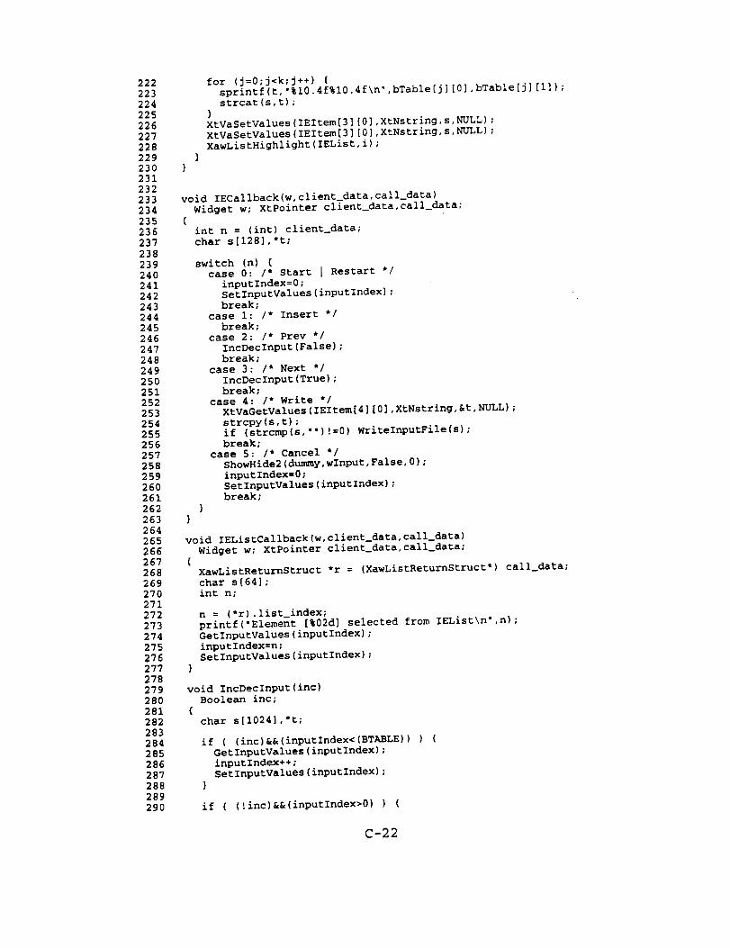
222
223
224
225
226
227
228
229
230
231
232
233
234
235
236
237
238
239
240
241
242
243
244
245
246
247
248
249
250
251
252
253
254
255
256
257
258
259
260
261
262
263
264
265
266
267
268
269
270
271
272
273
274
275
276
277
278
279
280
281
282
283
284
_85
286
287
288
289
290
for (j=0;j<k;j÷÷) {sprintf(t,'%10.4f%10.4f\n',bTable[j] [0],bTable[j] [i]);
strcat(s,t);
)XtVaSetValues(IEItem[3][0],XtNstring,s,NULL);
XtVaSetValues(IEItem[3][O],XtNstring, s,NULL);
XawListHighlight(IEList,i);
void IECallback(w, client_data,call_data)
Widget w; XtPointer client_data,call_data;
{int n = (int) client data;
char s[128],*t;
switch (n) [
case 0: /* Start I Restart */
inputIndex=0;
SetInputValues(inputIndex);
break;
case i: /* Insert */
break;
case 2: /* Prev */
IncDeclnput[False);
break;
case 3: /* Next */
IncDecInput(True);
break;
case 4: /* Write */
XtVaGetValues(IEItem[4][0],XtNstring,&t,NULL);
strcpy(s,t);
if (strcmp(s,'')!=0) WriteInputFile(s);
break;
case 5: /* Cancel */
ShowHide2(dummy,wInput,False, 0);
inputIndex=0;
SetInputValues(inputlndex);
break;
)
void IEListCallback(w,client_data,call_data)
Widget w; XtPointer client_data,call_data;
[XawListReturnStruct *r = (XawListReturnStruct*) call_data;
char s[64];
int n;
n = (*r).list_index;
printf('Element [%02d] selected from IEList\n',n);
GetInputValues(inputIndex);
inputIndex=n;
SetInputValues(inputIndex);
void IncDecInput(inc)
Boolean inc;
{char s[1024],*t;
if ((inc)&&(inputlndex<(BTABLE))) {
GetInputValues(inputlndex);
inputIndex++;
SetInputValues(inputlndex);
]
if ( (!inc)&&(inputIndex>0) ) {
C-22

291
292
293
294
295
296
297
298
299
300
301
302
303
304
305
306
307
308
309
310
311
312
313
314
315
316
317
318
319
320
321
322
323
324
325
326
327
328
329
330
331
332
333
334
335
336
337
338
339
340
341
342
343
344
345
346
347
348
349
350
351
352
353
354
355
356
357
358
359
GetInputValues(inputIndex);
inputIndex--;
SetlnputValues(inputIndex);
))
void WriteInputFile(s)
char *s;
{FILE *f;
int i,j,k;
f = fopen(s,'w');
fprintf(f," &NAME\n');
fprintf(f,"
fprintf(f,"
fprintf(f, °
fprintf(f,"
fprintf(f,"
fprintf(f,"
fprintf(f,"
fprintf(f,"
fprintf(f,"
fprintf(f,"
fprintf(f,"
fprintf(f,"
fprintf(f,"
fprintf(f, °
fprintf(f,"
fprintf(f,"
fprintf(f,"
fprintf(f,"
fprintf(f,"
fprintf(f,"
fprintf(f,"
fprintf(f,"
fprintf(f, °
fprintf(f "
fprintf(f °
fprintf(f "
fprintf(f "
fprintf(f "
fprintf(f "
fprintf(f "
fprintf(f "
fprintf(f "
fprintf(f "
fprintf(f •
fprintf(f,"
TMAX z
I2tMBDA =
TPRINT =
NPUNCH =
NBL =
NDELX =
TPI =
PAM =
UNIT =
NINERT =
NPNPXT =
AT =
XP =
XIP =
XG =
XE =
GAMA =
TFREF =
TIGN =
RUFSUR =
DDRG =
DDHC =
AP IAT =
AFTOS =
FKPR =
ROPR =
CPR =
TOREF =
SIGP =
TPSCRI =
RREF =
PREF --
BREXP =
EBC =
EBEX =
%10.4f\n"
%10.4f\n"
%10.4f\n"
%10.4fkn"
%10.4fkn"
%10.4f\n"
%10.4f\n"
%10.4f\n"
%10.4fkn"
%10.4fkn"
%10.4f\n"
%10.4f\n"
%10.4f\n"
%10.4fkn"
%10.4fkn"
%10.4f\n"
%10.4f\n"
%10 4f\n"
%10 4fkn"
%10 4fkn"
%10 4fkn"
%10 4fkn"
%10 4fkn"
%10 4fkn"
%10 4f\n"
%10 4fkn"
%10 4fkn"
%10 4fkn"
%10 4fkn"
%10.4fkn"
%10.4fkn"
%10.4fkn"
%10.4f\n"
%10.4f\n"
%10.4fkn"
varValue 0]
varValue i]
varValue 2]
varValue 3]
varValue 4]
varValue 5]
varValue 6]
varValue 7]
varValue 8]
varValue 9]
varValue i0]
varValue ii]
varValue 12]
varValue 13]
,varValue[14]
varValue[15]
varValue[16]
varValue[17]
varValue[18]
varValue[19]
varValue[20]
varValue[21]
varValue[22]
varValue[23]
varValue[24]
varValue[25]
varValue[26]
varValue[27]
varValue[28]
varValue[29]
varValue[30]
varValue[31]
varValue[32]
varValue[33]
varValue[34]
fprintf(f,"
fprintf(f,"
fprintf(f,"
fprintf f,"
fprintf f,"
fprintf f,"
fprintf f,"
fprintf f,"
fprintf f,"
fprintf f,"
fprintf(f,"
fprintf(f,"
fprincf(f,"
fprintf(f,"
fprintf(f,"
fprintf(f,"
fprintf(f,"
fprlntf(f,"
fprintf(f,"
DE =
CM =
ALFAD =
EROAT =
EROEXP =
NIGTAB =
NAPDVX =
NDATA =
NPPR =
PZONE =
NRESRT =
DELTAT =
PCI =
GAMAN =
P I SUBK =
DELTTF =
DFSDT =
TIIN =
FCRIT =
%10.4f\n" varValue[35]
%10_4f\n',varValue[36]
%10.4f\n',varValue[37]
%10.4f\n',varValue[38]
%10.4f\n',varValue[39]
%10.4f\n',varValue[40]
%10.4f\n',varValue[41]
%10.4f\n',varValue[42]
%10.4f\n',varValue[43]
%10.4f\n',varValue[44]
%10.4fkn °
%10.4fkn"
%10.4f\n"
%10.4fkn"
%10.4fkn"
%10.4fkn"
%10.4fkn"
%10.4f\n °
%10.4fkn"
varValue[45]
varValue[46]
varValue[47])
varValue[48])
varValue[49])
varValue[50])
varValue[51])
varValue[52])
varValue[53])
C-23

36O
361
362
363
364
365
366
367
368
369
370
371
372
373
374
375
376
377
378
379
38O
381
382
383
384
1
2
3
4
5
6
7
8
9
10
11
12
13
14
15
16
17
18
19
2O
21
22
23
24
25
26
27
28
29
30
31
32
33
34
35
36
37
38
39
4O
41
42
43
44
fprintf(f," POPEN =
fprintf(f," DELFAC =
fprintf(f," CHC =
fprintf(f," BFI =
fprintf(f," DELTFF =
fprintf(f," &END\n');
%10.4f\n',varValue[54]);
%10.4f\n',varValue[55]);
%10.4fkn',varValue[56]);
%10.4f\n',varValue[57]);
%10.4f\n',varValue[58]);
for (i=0;i<varValue[NIGTAB];i++)
fprintf(f,'%10.4f%10.4f\n',iTable[j][0],iTable[j][l]);
for (i=0;i<varValue[NAPDVX];i++) {
fprintf(f,'%10.4f%10.4f%10.4f%10.4f',
gTable[j] [0],gTable[j] [l],gTable[j][2],gTable[j] [3]);
if (gTable[j][4]!=0) fprintf(f,'%10.4f',gTable[j] [4]);
if (gTable[j][5]!=0) fprintf(f,'%10.4f',gTable[j] [5]);
fprintf(f,'kn');
)
for (i=0;i<varValue[NDATA];i++)
fprintf(f,'%10.4f%10.4f\n',bTable[j][0],bTable[j][l]);
fclose(f);
xplot.c
*/
# include "xpIncs. h"
#include "xpDefs. h"
#include "xpwidgets. h"
# include "xpgenera I. h"
# include "xpmenus. h"
# inc I ude "xpcommands. h"
# include "xplnput. h"
#include "xpdata. h"
# include "xpformats. h"
#include "xpplots .h"
#include "xpgeometry.h"
void main (argc, argv)
int argc; char **argv;
{
FILE *fi;
static XtActionsRec xplotActions[] = {
('idle", Idle},
{ •doKey •, DoKey),
{ "redrawPlot", RedrawPlot },
{ "saveConunand", SaveCommand ),
( •recal iCommand", RecallCommand},
{ "resizePlot", ResizePlot},
{ •resizeGeometry", ResizeGeometry},
{" exposeGeometry", ExposeGeometry},
[ •accept InputEntry", AcceptInputEntry},
};
XtAppContext app_context ;
int i ;
fi = fopen('XPlot.dat','w');
topLevel = XtVaAppInitialize {&app_context, "XPlot ",NULL, 0,
&argc, argv, NULL, NULL ) ;
XtAppAddActions (app_context, xplotActions, XtNumber (xplotActions) ) ;
CreateWidgets ( ) ;
XtReal i zeWidget (topLevel ) ;
C-24

454647484950515253545556575859
606162636465666768691234567891011121314151617181920
212223242526272829303132333435363738394041424344
screen =XtScreen(topLevel);display=XtDisplay(topLevel);
LoadFonts();LoadColors(};InitData();InitGCs();for(i=0;i<MAXPLOTS;i++)
InitFormat(i);LoadInputData();
SetFEValues(0);SetStatusLabel();
ChangeMGLabels(0);
printf('\n');
XtInstallAccelerators(rootPane,cliText);XtInstallAccelerators(cliLabel,cliText);
XtAppMainLoop(app context);
)
/*
xpMenus.c
"/
#include "xpIncs.h"#include "xpDefs.h"
#include "xpwidgets.h"#include "xpgeneral.h"#include "xpcommands.h"#include "xpdata.h"#include "xpformats.h"#include "xpplots.h"
/* $1: Global variables - (none) */
/* $2: Local variables - (none) */
/* $3: Global functions */
void MenuSelect();void CommandSelect();void VerbCallback();void SFCallback();void SFGetFile();void SelectString();void ShowHide2();void Loadlnput();void FileCallback();void ExecCallback();
/* $4: Local functions */void SetStatusLabel();void RunExec();
/* $5: Implementation =============================================== */
void MenuSelect(w,client data,call_data)Widget w; XtPointer client data,call_data;
{int menuData = (int) client_data;int menuNum, itemNum;
C-25

45
46
47
48
49
50
51
52
53
54
55
56
57
58
59
60
61
62
63
64
65
66
67
68
69
70
71
72
73
74
75
76
77
78
79
80
81
82
83
84
85
86
87
88
89
90
91
92
93
94
95
96
97
98
99
100
101
102
103
104
105
106
107
108
109
110
111
112
113
char s[64],*t;
FILE *f;
menuNum = menuData/HIWORD;
itemNum = menuData%HIWORD;
switch(menuNum) (
case IDMenuFile:
switch(itemNum) {
case 0:
ShowHide2(dummy,wFile,True,0);
break;
case i:
XtVaGetValues(menuText,XtNstring,&t,NULL);
strcpy(s,t);
f = fopen(s,'r');
if (f!=NULL)XtVaSetValues(fileText,XtNstring,s,XtNtype,XawAsciiFile,NULL);
break;
case 2:
ShowHide2(dummy,wFile,True,0);
break;
case 3:
break;
case 4:
XtVaGetValues(menuText,XtNstring,&t,NULL);
strcpy(s,t);
f = fopen(s,'w');
XtVaGetValues(fileText,XtNstring,&t,NULL) ;
fprintf(f,'%s',t);
fclose(f);
case IDmFileQuit:
exit(0);
)
break;
case IDMenuInpu:
switch (itemNum) {
case IDmInpuSet:
SelectString(0);
break;
case IDmInpuLoad:
LoadInput();
break;
case IDmInpuLoadSF:
SelectString(0);
LoadInput();
break;
case 4:
ShowHide2(dummy,wInput,True,0);
break;
)
break;
case IDMenuExec:
switch (itemNum) [
case IDmExecSetup:
ShowHide2(dummy,wExecute,True,0);
break;
case IDmExecRun:
RunExec();
break;
)
break;
case IDMenuData:
switch(itemNum) (
case IDmDataSet:
SelectString(1);
break;
case IDmDataLoad:
LoadData(dsName);
C-26

114
115
116
117
118
119
120
121
122
123
124
125
126
127
128
129
130
131
132
133
134
135
136
137
138
139
140
141
142
143
144
145
146
147
148
149
150
151
152
153
154
155
156
157
158
159
160
161
162
163
164
165
166
167
168
169
170
171
172
173
174
175
176
177
178
179
180
181
182
break;
case IDmDataLoadSF:
SelectString(1); .
LoadData(dsName);
break;
case IDmDataView:
ShowHide2(dummy,wData,True,0);
break;
case IDmDataPrint:
PrintData('ofile.dat');
break;
}break;
case IDMenuForm:
switch(itemNum) {
case IDmFormSet:
SelectString(2);
break;
case IDmFormLoadSF:
SelectString(2);
break;
)break;
case IDMenuPlot:
switch (itemNum) {
case IDmPlotSet:
SelectString(3);
break;
case IDmPlotInc:
IncDecPlot(True);
break;
case IDmPlotDec:
IncDecPlot(False);
break;
)break;
case IDMenuWind:
switch (itemNum) {
case 0:
ShowHide2(dummy,wWindowManager,True,0);
break;
case i:
ShowHide2(dummy,wFile,True,0);
break;
case 2:
ShowHide2(dummy_wInput,True,0);
break;
case 3:
ShowHide2(dummy,wExecute,True,0);
break;
case 4:
ShowHide2(dummy,wData,True,0);
break;
case 5:
ShowHide2(dummy,wForma_,True,0);
break;
case 6:
ShowHide2(dummy,wFormatAxes,True,0);
break;
case 7:
ShowHiae2(dummy,wFormatLines,True,0);
break;
case 8:
ShowHide2(dun_y,wFormatCurveFits,True,0);
break;
case 9:
ShowHide2(du_my,wPlotManager,True, O);
break;
case i0:
C-27

183
184
185
186
187
188
189
190
191
192
193
194
195
196
197
198
199
200
201
202
203
204
2O5
206
207
208
209
210
211
212
213
214
215
216
217
218
219
220
221
222
223
224
225
226
227
228
229
230
231
232
233
234
235
236
237
238
239
240
241
242
243
244
245
246
247
248
249
25O
251
ShowHide2(dtumny,wMotorGeometry,True,0);
break;
case ii:
ShowHide2(dtumny,wMotorConfiguration,True,0);
break;
}break;
}}
void CommandSelect(w. client data,call_data)
Widget w; XtPointer client_data,call_data;
{int commNum = (int) cllent_data;
char s[64];
static Boolean up[l] = {False};
switch (commNum)
{case 0:
ShowHide2(dummy.wWindowManager,True,0);
break;
case i:
ShowHide2(dummy,wFile,True,0);
break;
case 2:
ShowHide2(dummy,wlnput,True,0);
break;
case 3:
ShowHide2(dummy,wExecute,True,0);
break;
case 4:
ShowHide2(dummy,wData,True. O);
break;
case 5:
ShowHide2(dummy,wFormat,True.0);
break;
case 6:
ShowHide2(dummy.wFormatAxes. True,0);
break;
case 7:
ShowHide2(dummy,wFormatLines,True,0);
break;
case 8:
ShowHide2(dummy,wFormatCurveFits.True,0);
break;
case 9 :
ShowHide2(dummy,wPlotManager,True,0);
break;
case 10:
ShowHide2(dummy,wMotorGeometry,True,0);
break;
case ii:
ShowHide2(dummy,wMotorConfiguration.True,0);
break;
)}
void ShowHide2(w, id.show.code)
Widget w; int id; Boolean show; int code;
{char s[64];
if ((id>=0)&&(id<8)&&(plotExists[id])) {
if (show) {
windowUp[id]=True;
XtPopup(plotShell[id],XtGrabNone);
)else {
C-28

252
253
254
255
256
257
258
259
260
261
262
263
264
265
266
267
268
269
270
271
272
273
274
275
276
277
278
279
28O
281
282
283
284
285
286
287
288
289
290
291
292
293
294
295
296
297
298
299
300301
302
303
304
305
306
307
308
309
310
311
312
313
314
315
316
317
318
319
320
windowUp[id]=False;
XtPopdown(plotShell[id]);
))switch (id) {
case wWindowManager:
if (!windowUp[id]) {
strcpy(s,'Hide Window Manager');
XtPopup(commandSheil,XtGrabNone);
)else (
strcpy(s,'Show Window Manager');
XtPopdown(commandShell);
)XtVaSetValues{c[O],XtNlabel,s,NULL);
XtVaSetValues(mEntry[6] (0],XtNIabel,s,NULL);
windowUp[id]=!windowUp[id];
break;
case wFile:
if (!windowUp[id]) {
strcpy(s,'Hide File Editor');
XtPopup(fileShell,XtGrabNone);
)else (
strcpy{s,'Show File Editor');
XtPopdown(fileShell);
)XtVaSetValues(c[l],XtNlabel,s,NULL);
XtVaSetValues(mEntry[6][l],XtNlabel,s,NULL);
windowUp[id]= !windowUp[id];
break;
case wlnput:
if (!windowUp[id]) (
strcpy(s,'Mide Input File Editor');
XtPopup(IEShell,XtGrabNone);
}else {
strcpy(s,'Show Input File Editor');
XtPopdown(IEShell);
)XtVaSetValues(c[2],XtNlabel,s,NULL);
XtVaSetValues(mEntry[6][2],XtNlabel,s,NULL);
windowUp[id]= !windowUp[id];
break;
case wExecute:
if (!windowUp[id]) {
strcpy(s,'Hide Execution Setup');
XtPopup(execShell,XtGrabNone);
)else {
strcpy(s,°Show Execution Setup');
XtPopdown(execShell);
)XtVaSetValues(c[3],XtNlabel,s,NULL);
XtVaSetValues(mEntry[6][3],XtNlabel,s,NULL);
windowUp[id]= !windowUp[id];
break;
case wData:
if (!windowUp[id]) (
strcpy(s,'Hide Current Dataset');
XtPopup(dataShell,XtGrabNone);
)else (
strcpy(s,'Show Current Dataset');
XtPopdown(dataShell);
)XtVaSetValues(c[4],XtNlabel,s,NULL);
XtVaSetValues(mEntry[6][4],XtNlabel,s,NULL};
windowUp[id]=!windowUp[i_];
C-29

321
322
323
324
325
326
327
328
329
330
331
332
333
334
335
336
337
338
339
340
341
342
343
344
345
346
347
348
349
350
351
352
353
354
355
356
357
358
359
360
361
362
363
364
365
366
367
368
369
370
371
372
373
374
375
376
377
378
379
380
381
382
383
384
385
386
387
388
389
break;
case wFormat:
if (!windowUp[id]) {
strcpy(s.'Hide Format');
XtPopup(FEShell. XtGrabNone);
}else {
strcpy(s.'Show Format');
XtPopdown(FEShell);
}XtVaSetValues(c[5],XtNlabel,s.NULL);
XtVaSetValues(mEntry[6] [5],XtNlabel,s,NULL);
windowUp[id]=!windowUp[id];
break;
case wFormatAxes:
break;
case wFormatLines:
if (!windowUp[id]) {
strcpy(s,'Hide Format Lines');
XtPopup(DAShell,XtGrabNone);
}else {
strcpy(s,'Show Format Lines');
XtPopdown(DAShell);
)XtVaSetValues(c[7],XtNlabel,s,NULL);
XtVaSetVaiues(mEntry[6] [7].XtNIabel.s,NULL);
windowUp[id]=!windowUp[id];
break;
case wFormatCurveFits:
if (!windowUp[id]) (
strcpy(s,'Hide Format Curve Fits');
XtPopup(CFShell,XtGrabNone);
)else (
strcpy(s,'Show Format Curve Fits');
XtPopdown(CFShell);
)XtVaSetValues(c[8],XtNlabel,s,NULL);
XtVaSetValueslmEntry[6J[SJ,XtNlabel,s,NULL);
windowUp[id]=!windowUD[id];
break;
case wPlotManager:
if (!windowUp[id]) {
strcpy(s,'Hide Plot Manager");
XtPopup(PMShell,XtGrabNone);
)else (
strcpy(s.'Show Plot Manager");
XtPopdown(PMShell);
)XtVaSetValues(c[9],XtNlabel.s,NULL);
XtVaSetValues(mEntry[6][9].XtNlabel.s,NULL);
windowUp[id)=!windowUp[id_;
break;
case wMotorGeometry:
if (!windowUp[id]) {
strcpy(s,'Hide Motor Geometry');
XtPopup(MGShell,XtGrabNone);
)else {
strcpy(s,'Show Motor Geometry');
XtPopdown(MGShell);
)XtVaSetValues(c[10].XtNlabel,s,NULL);
XtVaSetValues(mEntry[6][10],XtNlabel,s,NULL);
windowUp[id]=!windowUp[id];
break;
case wMotorConfiguration:
C-30

390
391
392
393
394
395
396
397
398
399
40O
401
402
403
404
405
406
407
408409
410
411
412
413
414
415
416
417
418
419
420
421
422
423
424
425
426
427
428
429
430
431
432
433
434
435
436
437
438
439
440
441
442
443
444
445
446
447
448
449
450451
452
453
454
455456
457
458
if (!windowUp[id]) {
strcpy(s,'Hide Motor Configuration');
XtPopup(MGPictShell,XtGrabNone);
)else {
strcpy(s,'Show Motor Configuration');
XtPopdown(MGPictShell);
)XtVaSetValues(c[ll],XtNlabel,s,NULL);
XtVaSetValues(mEntry[6] [II],XtNIabel,s,NULL);
windowUp[id]=!windowUp[id];
break;
)
)
void VerbCallback(w,client_data,call data)
Widget w; XtPointer client_data,call_data;
{XawListReturnStruct *r = (XawListReturnStruct*) call_data;
strcpy(cli, (*r).string);
XtVaSetValues(cliText,XtNstring, cli,NULL);
XawTextSetInsertionPoint(cliText,strlen(cli));
)
/*
void SFCallback(w,client_data,call_data)
Widget w; XtPointer client data,call_data;
(int action = (int) client_data;
char filename[32],s[64];
String f;
f = XawDiaiogGetValueString(sfDialog);
strcpy(filename, f);
XtPopdown(sfGetFileShell);
switch (action) (
case SFCommCancel:
break;
case SFCommLoad:
sprintf(s,'The filename selected was:
break;
case SFCommSave:
break;
%s\n',filename);
))
void SFGetFile()
(XtPopup(sfGetFileShell,XtGrabNone);
)*/
void SelectString(code)
int code;
[char s[64],*ss;
int i;
XtVaGetValues(menuText,XtNstring,&ss,NULL);
strncpy(s,ss,63);
s[63]='\0';
if(s[0]!='\0') {
switch (code) {
case 0:
C-31

459
460
461
462
463
464
465
466
467
468
469
470
471
472
473
474
475
476
477
478
479
480
481
482
483
484
485
486
487
488
489
490
491
492
493
494
495
496
497
498
499
500
501
502
503
504
505
506
507
508
509
510
511
512
513
514
515
516
517
518
519
520
521
522
523
524
525
526
527
strcpy(inName,s);
break;
case i:
strcpy(dsName,s);
break;
case 2:
strcpy(pfName,s);
break;
case 3:
i=atoi(s);
if((i>=0)&&(i<=7)&&(plotExists[i]))
activePlot=i;
sprintf(plName,'%d',i);
)break;
)SetStatusLabel();
void SetStatusLabel()
{char s[256];
strcpy(s,'I: <');
strcat(s,inName);
strcat(s,'> D: <');
strcat(s,dsName);
strcat(s,'> F: <');
strcat(s,pfName);
strcat(s,'> p: 4");
strcat(s,plName);
strcat(s,'>');
XtVaSetValues(statusLabel,XtNlabel,s,NULL);
)
void FileCallback(w, client_data,call_data)
Widget w; XtPointer client_data,call_data;
(int n = (int) client_data;
FILE *f;
char s[128],*t;
XtVaGetValues(fileEntry[3],XtNstring,&t,NULL);
strcpy(s,t);
XtVaGetValues(fileText,XtNstring,&t,NULL);
switch (n) [
case 0:
ShowHide2(dummy,wFile,False,0);
break;
case i:
f = fopen(s,'w');
fprintf(f,'%s',t);
fclose(f);
break;
case 2:
f = fopen(s,'r');
if (f!=NULL)
XtVaSetValues(fileText,XtNstring,s,XtNtype,XawAsciiFile,NULL);
break;
)
void LoadInput()
{
C-32

52852953053153253353453553653753853954O54154254354454554654754854955055155255355455555655755855956O56156256356456556656756856957057157257357457557657757857958058158212345678910111213
14
FILE *fi;char s[128],*t;
XtVaGetValues(fileEntry[3],XtNstring,&t,NULL);
strcpy(s,t);
fi = fopen(s,°r°);if (fi!=NULL) {
XtVaSetValueslfileText,XtNstring, s,XtNtype,XawAsciiFile,NULL);)
)
void ExecCallback(w,client_data,call.data)Widget w; XtPointer client_data,cali_data;
{int n = (int) client_data;
switch (n) (case 0 :
ShowHide2(dummy,wExecute,False,0);break;
case l:break;
case 2:RunExec();break;
)
]
void RunExec ()(
char s[128],t[128],*u;
XtVaGetValues(execItem[l][0],XtNstring,&u,NULL);
strcpy(s,u);XtVaGetValues(execItem[l][l],XtNstring,&u,NULL);
strcpy(t,u);strcat(s,t);strcat(s," &');XtVaGetValues(execItem[l][2],XtNstring,&u,NULL);strcpy(t,u) ;if (strlen(t)!=0) {strcat(s," <');
strcat(s,t);)XtVaGetValues(execItem[l][3],XtNstring,&u,NULL);
strcpy(t,u);if (strlen(t)!=0) (strcat(s," >') ;strcat(s,t);
)system(s);
}/*
xpPlots.c....................... . ...............................................
*/
#include "xpIncs.h"#include "xpDefs.h"
#include "xpwidgets.h"#include "xpgeneral.h"#include "xpdata.h"#include "xpformats.h"
C-33

15161718192021222324252627
2829
3O3132333435
363738394041424344454647484950515253545556575859606162636465666768697071727374757677787980818283
/* $i: Global Variables */
unsigned long lineColor[64];unsigned long curvColor[32];
int activePlot=-l;
Boolean plotExists[MAXPLOTS];Boolean useCoI[MAXPLOTS][2*MAXCOLS];Boolean planar[MAXPLOTS]=(True,True,True,True,True,True,True,True};
/* $2: Local variables */
XSegment Grid[MAXPLOTS]'[50];
XPoint pt[MAXPLOTS][2*MAXCOLS][MAXPLANES]';XPoint pt2[MAXPLOTS][2*MAXCOLS][128];
char xLabels[MAXPLOTS][24][16];
char yLabels[MAXPLOTS][24][16];char zLabels[MAXPLOTS][24][16];
Dimension oldWidth[MAXPLOTS] =[640,640,640,640,640,640,640,640};
Dimension oldHeight[MAXPLOTS]=(480,480,480,480,480,480,480,480};
/* $3: Global functions */
void MakePlot();void KillPlot();void ActivatePlot();void RedrawPlot();void RedrawPlot2();void ResizePlot();void PMActiveCallback();void PMCreateCallback();void PMShowHideCallback{);void PMPlanarCallback();void PMActionCallback();void IncDecPlot();
/* $4: Local functions */
void RecreatePlot();
void SetupGrid();void SetupAxisLabels();void SetupPoints();
void DrawGrid();void DrawAxisLabels();void DrawPlotLabels();void DrawLegend();void DrawPoints();
void SmoothAxisValues();
void GESCP();void poly();void spline{);
/* $5: Implementation =============================================== */
void PMActiveCallback(w,clientdata,call_data)Widget w; XtPointer client_data,call data;
{int n = (int) XawToggleGetCurrent(PMitem[0][0]);
if ((n>=l)&&(n<=8))activePlot=n-l;
}
C-34

84858687888990919293949596979899
100101102103104105106107108109110111112113114115116117118119120121122123124125126127128129130131132133134135136137138139140141142143144145146147148149150151152
void PMCreateCallback(w, client_data,call_data)Widget w; XtPointer client_data,call_data;
(int p = (int) client_data;
if ((!plotExists[p])&&(dataLoaded)) {XtVaSetValues(PMitem[0] [p],XtNsensitive,True,NULL);XtVaSetValues(PMitem[1] [p],XtNlabel,'Destroy',NULL);XtVaSetValues(PMitem[2][p],XtNsensitive,True,XtNlabel,'Hide',NULL);MakePlot(p);ShowHide2(plotShell[p],p,True,0);
)else if (plotExists[p]) { .
KillPlot(p);XtVaSetValues(PMitem[0] [p],XtNsensitive,False,NULL);XtVaSetValues(PMitem[l][p],XtNlabel,'Create',NULL);
XtVaSetValues(PMitem[2][p],XtNsensitive,False,XtNlabel,'Show',NULL);}
}
void PMShowHideCallback(w,client_data,call_data)
Widget w; XtPointer client_data,call_data;{
int p = (int) client data;
if (windowUp[p]) {XtVaSetValues(PMitem[2][p],XtNlabel,'Show',NULL);ShowHide2(plotShell[p],p,False, 0);
)else {
XtVaSetValues(PMitem[2][p],XtNlabel,'Hide',NULL);ShowHide2 (plotShell [p] ,p,True, 0) ;
)
)
void PMPlanarCallback (w, client_data, calldata)Widget w; XtPointer client_data,call_data;
{int which = (int) client_data;
if ((activePlot>=0)&&(activePlot<MAXPLOTS)) (if (planar[activePlot]) (
planar[activePlot] = False;XtVaSetValues(PMitem[3][0],XtNlabel,'Plane Plot',NULL);
)else {
planar[activePlot]=True;XtVaSetValues(PMitem[3][0],XtNlabel,'Space Plot',NULL);
)CopyData(activePlot);StatData(activePlot);
/* PrintPlotData(activePlot); */SetupGrid(activePlot);SetupAxisLabels(activePlot);SetupPoints(activePlot);RedrawPlot2(activePlot);
)) - _
void PMActionCallback(w, client_data,call_data}
Widget w; XtPointer client_data,call_data;{
int commNum = (int) client_data;
switch (commNum) [case i:
IncDecPlot{True);break;
case 2:
C-35

153154155156
157158159160161162163164165166167168169170171172173174175176177178179180181182183184185186187188189190191192193194195196197198199200201202203204205206207208209210211212213214215216217218219220
221
IncDecPlot(False);break;
case 3:if ((activePlot>=0)&&(activePlot<=7)) (
if (planar[activePlot])while (currentPlane[activePlot]<(numPlanes-l))
IncDecPlot(True);else
while (currentRow[activePlot]<(numRows-l))IncDecPlot(True);
)break;
case 4:if ((activePlot>=0)&&(activePlo_<=7)) {
if (planar[activePlot])while (currentPlane[activePlot]>0)
IncDecPlot(False);
elsewhile (currentRow[activePlot]>0)
IncDecPlot(False);
break;case 5:
ShowHide2(dummy,wFormat,True,0);break;
case 6:ShowHide2(dununy,wPiotManager,True,0);break;
void MakePlot(p)int p;
{plotExists[p]=True;
if(dataLoaded) (
CopyData(p);StatInd();
StatData(p);/* PrintPlotData(p); */
SetupGrid(p);SetupAxisLabels(p);SetupPoints(p);ActivatePlot(p);
)else
printf('No dataset currently loaded\n');
void KillPlot(p)int p;
(ShowHide2(dunm_,wPlot0+p,False,0);windowUp[wPlot0+p]=False;plotExists[p]=False;if (p==activePlot) {
XawToggleUnsetCurrent(PMitem[0][0]);activePlot=-l;
)
void ActivatePlot(p)int p;
{if((p>=0)&&(p<MAXPLOTS)&&(plotExists[p]))
activePlot = p;
XawToggleSetCurrent(PMitem[0] [0],(caddr_t) p+l);
C-36

222
223
224
225
226
227
228
229
230
231
232233
234
235
236
237
238
239240
241
242
243
244
245
246
247248
249
250
251
252
253
254
255
256
257258
259
260
261
262
263
264
265
266
267
268269
270
271
272
273
274275
276
277
278
279
280
281
282
283
284285
286
287
288
289
29O
if (planar[activePlot])
XtVaSetValues(PMitem[3][0],XtNlabel,'Space Plot',NULL);
else
XtVaSetValues(PMitem[3] [0],XtNlabel,"Plane Plot",NULL);
))
void RedrawPlot (w, event, params, numParams)
Widget w; XEvent *event; String *params;
[XExposeEvent *myevent = (XExposeEvent*)
Window wind=XtWindow(w);
static int i=0; ,.
int p = atoi(params[0]);
if ((*myevent).count==0) {
i+÷;
XClearWindow(display,wind);
DrawGrid(p);
DrawAxisLabels(p);
DrawPlotLabels(p);
DrawLegend(p);
DrawPoints(p);
printf(':RedrawPlot(%d) - #%d\n',p,i);
))
void RedrawPlot2 (p)
int p;
(Window wind=XtWindow(plot[p]);
XClearWindow(display,wind);
DrawGrid(p);
DrawAxisLabels(p);
DrawPlotLabels(p);
DrawLegend(p);
DrawPoints(p);
)
void ResizePlot(widget,event,params,numParams)
Widget widget; XEvent *event; String *params;
{Dimension w,h;
int p = atoi(params[0]);
XtVaGetValues(plotShell[p],XtNwidth,&w,XtNheight,&h,NULL);
/* printf(':ResizePlot(%d) - (%d,%d)\n',p,w,h) ; */L
f[p].width = w;
f[p].height = h;
if ((w!=oldWidth[p])[l(h!=oldHeight[p])) {
RecalcFozm%at(p);
SetupGrid(p);
SetupPoints(p); .....
)if ((w<=oldWidth[p])&&(h<=oldHeight[p]))
RedrawPlot2(p);
oldWidth[p] =w;
oldHeight[p]=h;
)
void IncDecPlot(inc|
Boolean inc;
(Boolean changed=False;
Cardinal *numParams;
event;
Cardinal *numParams;
C-37
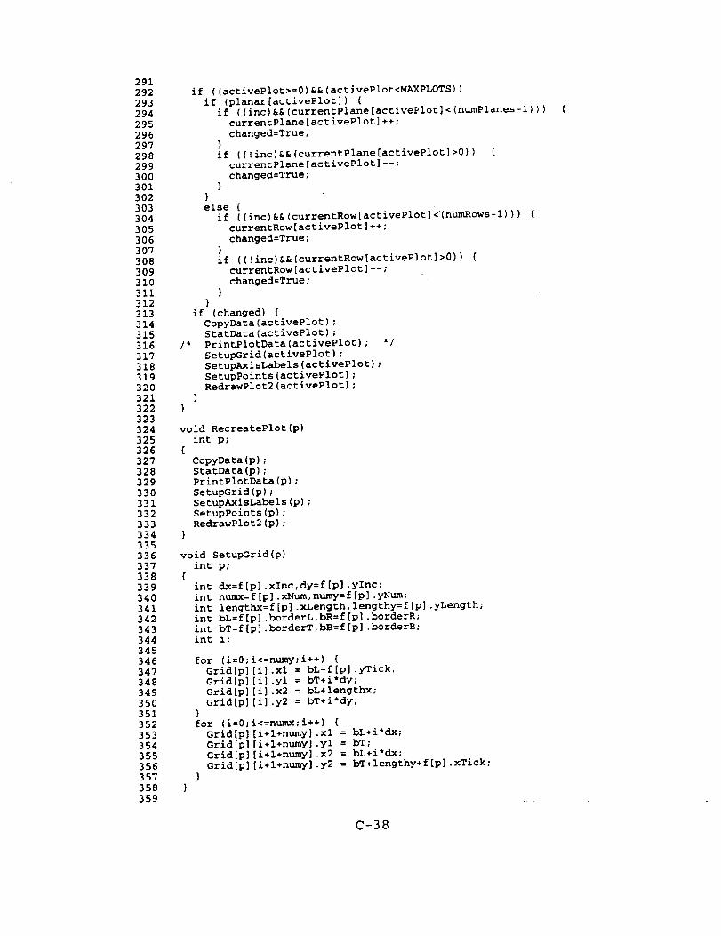
291
292
293
294
295
296
297
298
299
300
301
302
303
304
3O5
306
307
308
309
310
311
312
313
314
315
316
317
318
319
320
321
322
323
324
325
326
327
328
329
330
331
332
333
334
335
336
337
338
339
340
341
342
343
344
345
346
347
348
349
350
351
352
353
354
355
356
357
358
359
if ((activePlot>=0)&&(activePlot<MAXPLOTS))
if (planar[activePlot]) (
if ((inc)&&(currentPlane[activePlot]<(numPlanes-1)))
currentPlane[activePlot]÷+;
changed=True;
)
if ((!inc)&&(currentP1ane[activeP1ot]>0)) (
currentP1ane[activePlot]--;
changed=True;
}
}
else {
if ((inc)&&(currentRow[activePlot]<'(numRows-l))) [
currentRow[activePlot]++;
changed=True;
)
if ((!inc)&&(currentRow[activePlot]>O)) (
currentRow[activePlot]--;
changed=True;
}
/*
)
)
)
if (changed) {
CopyData(activePlot) ;
StatData(activePlot) ;
PrintPlotData(activePlot);
SetupGrid(activePlot);
SetupAxisLabels(activePlot);
SetupPoints(activePlot);
RedrawPlot2(activePlot);
void RecreatePlot(p)
int p;
{
CopyData(p);
StatData(p);
PrintPlotData(p);
SetupGrid(p);
SetupAxisLabels(p);
SetupPoints(p);
RedrawPlot2(p);
}
void SetupGrid(p)
int p;
{
int dx=f[p].xInc,dy=f[p].ylnc;
int numx=f[p].xNum, numy=f[p].yNum;
int lengthx=f[p].xLength, lengthy=f[p].yLength;
int bL=f[p].borderL,bR=f[p].borderR;
int bT=f[p].borderT,bB=f[p].borderB;
int i;
for (i=0;
Grid[p]
Grid[p]
Grid[p]
Grid[p]
}
for (i=0;
Grid[p]
Grid[p]
Grid[p]
Grid[p]
)
i<=numy;i++) {
[i].xl = bL-f[p].yTick;
[i].yl = bT+i*dy;
[i].x2 = bL+lengthx;
[i].y2 = bT+i*dy;
i<=numx;i++) (
[i+l÷numy].xl = bL+i*dx;
[i÷l+numy].yl = bT;
[i+l+numy].x2 = bL+i*dx;
[i+l+numy].y2 = bT+lengthy+f[p].xTick;
C-38

36036136236336436536636736836937037137237337437537637737837938O381
382
383
384
385
386
387
388
389
390
391
392
393
394
395
396
397
398
399
400
401
402
403
404
405
406
407
408
409
410
411
412
413
414
415
416
417
418
419
420
421
422
423
424
425
426
427
428
void DrawGrid (p)
int p ;
[Window wind=XtWindowlplot[p]) ;
XSetForeground (display,gc [0], rColor [Black] .pixel) ;
XDrawSegmen t s (di splay, wind, gc [0 ], Gr i d [p ] , f [p ] .nGr id) ;
)
void SetupAxisLabels (p)
int p ;
(float temp, minx, miny, maxx, maxy, minz, max z, rangex, rangey, rangez ;
int numx=f [p] .xNum, numy=f [p] .yNum;
int i ;
char s[16],t[16];
sprintf (s, "%%%sf", f[p] .xFormat) ;
sprintf(t,'%%%sf',f[p].yFormat) ;
if (!f[p].opt[oAutoScale]) (
minx= f [p] .xMin;
maxx= f [p]. xMax;
rangex= f [p] .xMax- f [p] .xMin;
minz= f [p ] .xMin;
maxz= f [p ]. xMax;
rangez=f [p] .xMax- f [p] .xMin;
miny=f [p] .yMin;
maxy=f [p]. yMax;
rangey= f [p] .yMax- f [p] .yMin;
)else (
if (planar[p]) (
minx=xMin;
ma_=xMax;
rangex =xRange;
}else [
minz=zMin;
maxz=zMax;
rangez=zRange;
]miny'-yMin [p] ;
maxy=yMax [p] ;
rangey=yRange [p] ;
)
if (planar [p] ) (
for {i=0 ; i<=numx; i++) {
temp=minx+ i *rangex /numx;
sprintf (xLabels [p] [i] ,So temp) ;
}for (i=0 ; i<=numy; i++) (
temp=miny+ i *rangey /numy;
sprintf (yLabels [p] [i], t, temp) ;
))else (
for (i=0 ; i<=numx; i++) {
temp=min z + i *rangez /numx;
sprintf (xLabels [p] [i], s, temp) ;
}
for (i=0 ;i<=numy; i++) {
temp--miny+ i * rangey/numy;
sprintf (yLabels [p] [i], t, temp) ;
})
C-39

429
430
431
432
433
434
435
436
437
438
439
440
441
442
443
444
445
446
447
448
449
450
451
452
453
454
455
456
457
458
459
460
461
462
463
464
465
466
467
468
469
470
471
472
473
474
475
476
477
478
479
480
481
482
483
484
485
486
487
488
489
490
491
492
493
494
495
496
497
void DrawAxisLabels(p)
int p;
{Window wind=XtWindow(plot[p]);
int dx=f[p].xInc,dy=f[p|.yInc;
int maxx=f[p].xNum, maxy=f[p].yNum;
int i,w,x,y;
x=f[p].borderL;
y=f[p].borderT+f[p].yLength+f[p].xTick+12;
XSetForeground(display,gc[0],rColor[Black].pixel);
for(i=0;i<=maxx;i++) {
w=XTextWidth(fs6xl0,xLabels[p][i],strlen(xLabels[p][i]))/2;
XDrawString(display,wind,gc[0],x+i*dx-w,y,
xLabels[p][i],strlen(xLabels[p] [i]));
]x=f[p].borderL-f[p].yTick-6;
y=f[p].borderT+f[p].yLength;
for(i=0;i<=maxy;i++) {
w=XTextWidth(fs6xl0,yLabels[p] [i],strlen(yLabels[p] [i]));
XDrawString(display,wind,gc[0],x-w,y-i*dy,
yLabels[p][i],strlen(yLabels[p][i]));
)
void DrawPlotLabels(p)
int p;
(Window wind=XtWindow(plot[p]);
char t[64];
int w,n,h,v;
XSetForeground(display,gc[0],rColor[Black].pixel);
strcpy(t,f[p].title);
w=XTextWidth(fsHelvl8b,t,strlen(t));
h=f[p].borderL÷(f[p].xLength-w)/2;
v=f[p].borderT-8;
XDrawString(display,wlnd,gc[2],h,v,t,strlen(t));
if (planar[p])
sprintf(t,'Distance (inch) [Time = %6.0f : %3d/%3d]',
z[currentPlane[p]],currentPlane[p]+l,numPlanes);
else
sprintf(t,'Time (msec) [Dist = %6.0f : %3d/%3d]',
x[currentRow[p]],currentRow[p]+l,numRows);
w = XTextWidth(fs6xl0,t,strlen(t));
h=f[p].borderL÷(f[p].xLength-w)/2;
v=f[p].borderT+f[p].yLength+30;
XDrawString(display, wind,gc[0],h,v,t,strlen(t));
void DrawLegend(p)
int p;
(Window wind=XtWindow(plot[p]);
int j,k=-l;
XSegment Legend[l];
int len=15,xDist=100,yDist=14,x,y;
int test;
test = ( planar[p] ? MAXCOLS : 2*MAXCOLS );
XSetLineAttributes(display,gc[O],8,LineSolid,CapButt,JoinRound);
for(j=0;j<test;j++)
if (useCol[p][j]) {
k++;
x=f[p].borderL+(k%4)*xDist;
y=f[p].borderT+f[p].yLength+(k/4)*yDist+45;
Legend[0].xl=x;
C-40

4984995005015O25O35045O5506507508509510511512513514515
516517518519520521522523524525
526527528529530531532533534535536537538539540541542543544545546547548549550551552553554555556557558559560561562563564565566
Legend[0].yl=y-4;Legend[0].x2=x+len;Legend[0J.y2=y-4;XSetForeground(display,gc[0],rColor[Black].pixel);
XDrawString(display, wind,gc[O],x+len+5,y,columnNames[j],strlen(columnNames[j]));
XSetForeground(display,gc[0],lineColor[f[p].color[j]]);XDrawSegments(display,wind,gc[0],Legend, l);
)XSetForeground(display,gc[0],rColor[Black].plxel);XSetLineAttributes(display,gc[0],0,LineSolid,CapButt,JoinRound);
)
void SetupPoints(p)int p;
(int bL=f[p].borderL,bR=f[p].borderR;int bT=f[p].borderT,bB=f[p].borderB;float minx=xMin,miny=yMin[p],minz=zMin;float rangex=xRange,rangey=yRange[p],rangez=zRange;int lengthx=f[p].xLength, lengthy=f[p].yLength;int i,j;
if (!f[p].opt[oAutoScale]) {minx=f[p].xMin;rangex=f[p].xMax-f[p].xMin;mlnz=f[p].xMin;rangez=f[p].xMax-f[p].xMin;miny=f[p].yMin;rangey=f[p].yMax-f[p].yMin_
)else (
if (planar[p]) (minx=xMin;
rangex=xRange;)else {
minz=zMin;rangez=zRange;
)miny=yMin[p];rangey=yRange[p];
)
if (planar[p]) {for(j=0;j<numCols;j++) {
if (useCol[p] [j])for(i=0;i<numRows;i++) (
pt[p][j][i].x=bL÷((x[i]-minx)/rangex)*lengthx;pt[p] [j] [i].y=bT÷lengthy-((plotData[p] [j][i]-miny)/
rangey)*lengthy;)
))else [
for(j=O;J<(2*MAXCOLS);J++) (if (useCol[p] [j])
for(i=0;i<ntunPlanes;i++) [pt[p][j][i].x=bL+((z[i]-minz)/rangez)*lengthx;pt[p][j][i].y=bT+lengthy-((plotData[p][j][i]-miny)/
rangey)*lengthy;)
))
void DrawPoints(p)int p;
(
C-41

567
568
569
570
571
572
573
574
575
576
577
578
579
580
581
582
583
584
585
586
587
588
589
590
591
592
593
594
595
596
597
598
599
600601
602
603
604
605
606
607
608
609
610
611
612
613
614
615
616
617
618
619
620
621
622
623
624
625
626
627
628
629
630
631
632
633
634
635
Window wlnd=XtWindow(plot[p]);
static char dashPattern[] = [16,8};
int j,test;
XRectangle r;
int bL=f[p].borderL,bR=f[p].borderR;
int bT=f[p].borderT,bB=f[p].borderB;
int lengthx=f[p].xLength,lengthy=f[p].yLength;
XSetLineAttributes(display,gc[0],4,LineOnOffDash,CapRound,JoinRound};
XSetDashes(display,gc[0],0,dashPattern, 2);
r.x=bL-2; r.y=bT-2; r.width=lengthx÷4; r.height=lengthy+4;
XSetClipRectangles(display,gc[0],0,0,r,l,Unsorted);
test=(planar[p] ? MAXCOLS : 2*MAXCOLS);
for(j=0;j<test;j++)
if (useCol[p] [j]) {
if (f[p].numDashes[j]>0) (
XSetLineAttributes(display, gc[0],4,LineOnOffDash,CapRound,JoinRound);
XSetDashes(display, gc[0],0,f[p].dashes[j],f[p].numDashes[j]);
)else
XSetLineAttributes(display,gc[O],4,LineSolid,CapRound,JoinRound);
XSetForeground(display,gc[0],lineColor[f[p].color[j]]);
if (planar[p])
XDrawLines(display,wind,gc[0],pt[p][j],numRows,CoordModeOrigin);
else
XDrawLines(display,wind,gc[O],pt[p][j],numPlanes,CoordModeOrigin);
}XSetForeground(display, gc[0],rColor[Black].pixel);
XSetLineAttributes(display,gc[0],0,LineSolid,CapButt,JoinRound);
XSetClipMask(display,gc[0],None);
void SmoothAxisValues(vMin,vMax)
float vMin,vMax;
{float vRange;
int a,al,a2,b,bl,b2;
vRange = vMax-vMin;
a = logl0(vRange);
al= a-l;
a2= a-2;
b = vRange/a;
printf('%d'.b);
)
/*
The following routines apply only to curve-fitting (not implemented)
*/
void GESCP(n,a,b)
int n; float a[10] [10],b[10] ;
{int i, j, k, p, nrow[10], ncopy;
float max,re°sum,s[10];
for (i=0;i<n;i++) {
max = -I.0E+I0;
for (j=0;j<n; j++)
if (fabs(a[i][j]) >max) max = fabs(a[i][j]);
C-42

);
636
637
638
639
640
641
642
643
644
645
646
647
648
649
650
651
652
653
654
655
656
657
658
659
660
661
662
663
664
665
666
667
668
669
670
671
672
673
674
675
676
677
678
679
680
681
682
683
684
685
686
687
688
689
690
691
692
693
694
695
696
697
698
699
700
701
702
703
s [i] =max;
nrow[i] =i;
)
for (i=0;i<(n-l);i++) {
max=-l.0E+10;
for (j=i; j<n; j++)
if ( (fabs{a[nrow[j]][i])/s[nrow[j]]) > max) {
max = fabs(a[nrow[j] ] [i])/s[nrow[j]} ;
p=j;
}
if (a[nrow[p]] [i]==0.0) printf('No unique
if (nrow[i] !=nrow[p] ) (
ncopy=nrow [i ] ;
nrow [i ] =nrow [p ] ;
nrow [p] =ncopy;
}
for (j=(i+l);j<n;j++) {
m = a[nrow[j]] [i]/a[nrow[i]] [i] ;
for (k=0;k<{n+l) ;k++)
a[nrow[j]] [k]=a[_row[j]] [k]-m*a[nrow[i]] [k] ;
)
) ......
if (a[nrow[n-l]] (n-l]==0.0) printf('No unique
b[n-l]=a[nrow[n-l]] [n]/a[nrow[n-l] ] (n-l] ;
for (i=(n-2);i>=0;i--) {
SUm=0 ;
for (j=i+l; j<n; j++)
sum=sum+a[nrow[i] ] [j] *b[j] ;
b[i] = (a[nrow[i]] [n]-sum)/a[nrow[i]] [i];
)
solution exists\n');
solution existskn');
void poly(n,m,x,y)
int n,m; float x[],y[];
(
int i,j,k;
float a[10][10],b[10],p[256],e[256],sum;
for (i=0;i<n;i++) {
for (j=0;j<n;j++) {
such=0;
for (k=0;k<m;k++)
sum=sum+( (i+j)==0 ? 1.0 : (float) pow((double) x[k],(double) i+j)
if ((i+j)==0) sum=m;
a[i] [j ]=sum;
)
)
for (i=0;i<n;i++) {
Sum=0;
for (k=0;k<m;k++)
stun=su_+y[k]*(i==0 ? 1.0 :
a[i] [n] =sum;
)
GESCP(n,a,b);
for (i=0;i<n;i++)
printf(°x[%d] = %12.6f\n',i,b[i]);
for (i=0;i<m;i++) {
Sum=0;
for(k=0;k<n;k++)
(float) pow{(double) x[k], (double) i) );
sum=sum+b[k]*(k==0 ? 1.0 : (float) pow((double) x[i],(double) k) );
p[i]=sum;
e[i]=y[i]-p[i];
printf('%12.6f %12.6f%12.6f%12.6f\n',x[i],y[i],p[i],e[i]);
}
sum=0;
for (i=0;i<m;i++)
sum+=(float) pow((double) e[i],(double) 2);
prlntf('\n\nTotal error = %12.6fkn',sum);
C-43

704705706
707708709710711712713714715716717718
71972072172272372472572672772B7297307317327337347357361234567B9I0ii12131415161718192O2122232425262728293O313233343536
void spline(n,x,y)int n; float x[],y[];
{int i,j;float a[256],b[256],c[256],d[256],
h[256],alpha[256],l[256],u[256],z[256];
for (i=0;i<=n;i÷+)a[i]=y[i];
for (i=0;i<n;i++)h[i]=x[i+l]-x[i];
for (i=l;i<n;i++)
alpha [i] =3" (a [i+l] *h [i-l] -a[i] * (x[i+l] -x[i-l] )+a[i-l] *h[i] )/(h[i-l]*h[i]);
i[0]=i;u[0]=0;z[0]=0;for (i=l;i<n;i++) [
l[i]=2*(x[i+l]-x[i-l])-h[i-l]*u[i-l];u[i]=h[i]/l[i];
z[i]=(alpha[i]-h[i-l]*z[i-l])/l[i] ;}l[n]=l.0;z[n]=0.0;c[n]=0.0;for (j=(n-l);j>=0;j--) {
c[j]=z[j]-u[j]*c[j+lJ;b[j] =(a[j+l] -a[j] )/h[j] -h[j]* (c[j+l]+2*c [j] )/3;d[j] = (c [j+l]-c [j] )/ (3*h[j]) ;
))
/*
xpWidgets.c
*/
#include "xpIncs.h"#include "xpDefs.h"
/* The following files have to be included for callback routines */
#include "xpmenus.h"#include "xpcommands.h"#include "xpinput.h"#include "xpformats.h"#include "xpplots.h"#include "xpgeometry.h"
/* $i: Global variables */
Widget topLevel;
Widget rootPane;Widget menuPane,menuText;Widget statusLabel;Widget commPane,verbViewport,verbList,commViewport,commList;Widget cliPane,cliLabel,cliText;
Widget mMenuButton[NUMMenus],mSimpleMenu[NUMMenus];Widget mEntry[NUMMenus][MAXENTRIES];
Widget con_nandShell,cormnandBox,c[NUMCommands];
Widget PMShell,PMForm, PMBox[4],PMTop[4],PMitem[4] [8];Widget infoShell,infoCore;
C-44
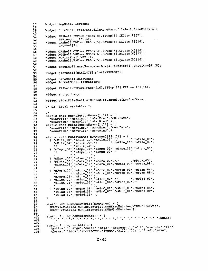
37
38
39
4O
41
42
43
44
45
46
47
48
49
50
51
52
5354
55
56
57
58
59
60
61
62
63
64
65
66
67
68
69
70
71
72
73
74
75
76
77
78
79
80
81
82
83
84
85
86
87
88
89
90
91
92
93
94
95
96
97
98
99
100
101
102
103
104
105
Widget
Widget
Widget
Widget
Widget
Widget
Widget
Widget
Widget
Widget
Widget
Widget
Widget
Widget
Widget
I* $2:
logShell,logText;
fileShell,filePane,fileMenuPane,fileText,fileEntry[4];
IEShell,IEForm, IEBox[8],IETop[8],IEItem[8] [2],
IEViewport,IEList;
DAShelI,DAForm,DABox[5],DATop[5],DAItem[5] [16],
DALabel[2];
CFShell,CFForm,CFBox[4],CFTop[4],CFItem[4][16];
MGShelI,MGForm,MGBox[6],MGTop[6],MGItem[6] [12];
MGPictShell,MGPict;
FAShelI,FAForm, FABox[5],FATop[5],FAItem[5] [16];
execShell,execForm, execBox[4],execTop[4],execItem[4] [8];
plotShelI[MAXPLOTS],plot[MAXPLOTS];
dataShell,dataText;
formatShell,formatText;
FEShelI,FEForm,FEBox[16],FETop[16],FEItem[16][16];
entry,dummy;
sfGetFileShell,sfDialog, sfCancel,sfLoad, sfSave;
Local variables */
/*
static char mMenuButtonNames[][12] = {
"mBarFile','mBarInpu','mBarExec','mBarData',
"mBarForm','mBarPlot','mBarWind',);
static char mSimpleMenuNames[][12] = {
"menuFile','menuInpu','menuExec",'menuData',
"menuForm','menuPlot','menuWind',);
static char mEntryNames[NUMMenus] [12][24] = {
( "mFile_00",'mFile_01","mFile_02",'/ • "mFile 03",a
{
{
};
{m/ w,
r
{ "mExec_00",
( "mData_00 • ,
"mData_04",w •
[ "mForm_00"
•/
"mForm_09"
"mPlot_00"
"mPlot_04"
"mWind_00"
"mWind_05"
"mWind_10"
"mFile_04",'mFile_05",'/ ",'mFile_06",'mFile_07 ",
• / ",'mFile_08"},
•mlnpu_00",'mInpu_01",'mInpu_02",•mInpu 03",'mlnpu 05 ",
"mInpu_06","mInpu_07"," "," ",
"mExec_01"),
"mData_01•,'mData_02",'/" ,•mData_03",
"mData_05",'mData_06",'mData_07",'mData_08",
w • }#
"reForm_01", 'reForm_02 •, "reForm_03", "reForm_04 •,
"reForm_05 •, 'mForm_06", "reForm_07", "reForm 08",
"reForm_f0" },
"mPlot_01",'mPlot_02",'/ ",'mPlot_03",
"mPlot_05",'mPlot_06",'mPlot_07",''
• • )t
•mWind_01",'mWind_02",'mWind_03",'mWind_04 • ,
"mWind_06",'mWind_07",'mWind_08",'mWind_09",
"mWind_ll" ],
static int numMenuEntries[NL_MMenus] = {
NUMFileEntries,NUMInpuEntries,NUMExecEntries,NUMDataEntries,
NUMFormEntries,NUMPlotEntries,Nl/MWindEntries ];
static String co_lements[] = (
. . u . . • ........ • • . • .......... '" _L}I , _ _ _ t w • • w a r I r , ;
static String verbs[] = {
"active','change','color','data','decrement','edit','execute','fit',
"format','hide','increment','input','kill','list','load','make',
C-45

106
107
108
109
ii0
iii
112
113
114
115
116
117
118
119
120
121
122
123
124
125
126
127
128
129
130
131
132
133
134
135
136
137
138
139
140
141
142
143
144
145
146
147
148
149
150
151
152
153
154
155
156
157
158
159
160
161
162
163
164
165
166
167
168
169
170
171
172
173
174
"plane','plot','print','quit','save',
"set','show','space','view',NULL,);
static String IEentries[] = (
• ",NULL};
*/
#define Nq]MFEOptions 2
#define NUMFECommandString 4
#define NUMFEAxesString 4
static char s[64],t[64];
/* $3: Global functions */
void CreateWidgets();
/* $4: Local functions - (none) */
/* $5: Implementation =============================================== */
void CreateWidgets()
Cstatic char mMenuButtonNames[] [I0] = [
"mBarFile','mBarInpu','mBarExec','mBarData',
"mBarForm','mBarPlot','mBarWind',};
static char mSimpleMenuNames[][10] = (
"menuFile','menuInpu','menuExec','menuData',
"menuForm','menuPlot','menuWind',};
static char mEntryNames[NUMMenus][12][12] = (
{ "mFile_00" "mFile_01",'mFile_02",'/ ........ ,'mFile_03",
•mFile_04" "mFile_05",'/ ........ ,'mFile_06",'mFile_07",
• / ......... mFile_08"},
( "mInpu_00" "mInpu_01",'mInpu_02",'mInpu_03",'mInpu_05",
• / ......... mInpu_06",'mInpu_07"," "," ",
{ "mExec_00" "mExec_01"},
{ "mData_00" "mData_01",'mData_02",•/ ....... ','mData 03",
•mData_04 ° °mData_O5",'mData_O6",'mData_O7",'mData_08",
l w • • )_
( "mYorm_00" "mYorm_01",•mForm_02•,'mYorm_03",'mForm_04 • ,
• / ......... mForm_05• •mForm_06..mForm_07.,.mForm 08 ,,
•mForm 09" "mForm_10" },
{ •mPlot_00" "mPlot_01",'mPlot_02",'/ ........ ,'mPlot 03",
"mPlot_04" "mPlot_05•,'mPlot_06",•mPlot_07", " ",
• • • • ) ,
{ •mWind_00" "mWind_01",'mWind_02",'mWind_03•,'mWind_04 ",
•mWind_05 • "mWind_06",'mWind_07",•mWind_08•,'mWind_09 • ,
•mWind_10" "mWind_ll" ),
);static int numMenuEntries[NUMMenus] = {
NUMFileEntries,NUMInpuEntries,NUMExecEntries,NiR4DataEntries,
NUMFormEntrles,NUMPlotEntries,NUMWindEntries );
static String commElements[] = {
, , , , , , , , , , , ,NULL};=
•active.,.change','color','data',-decrement',-edit•,•execute.,•fit ",
"format','hide','increment','input','kill','list','load','make',
•plane•,-plot','print','quit',•save','set ",
.show-,•space-,'view'.NULL,);
static String IEentries[] = {
• ",NULL);int i,j,total;
/* _Generate the pane that will serve as the root pane for the window */
rootPane =XtVaCreateManagedWidget('rootPane',panedWidgetClass,topLevel,
XtNorientation,XtorientVertical,
NULL);
C-46

175
176
177
178
179
180
181
182
183
184
185
186
187
188
189
190
191
192
193
194
195
196
197
198
199
2O0
201
202
203
204
205
206
207
208
209
210
211
212
213
214
215
216
217
218
219
220
221
222
223
224
225
226
227
228
229
230
231
232
233
234
235
236
237
238
239
240
241
242
243
/* A pane to hold all of the menu bar entries */
menuPane =XtVaCreateManagedWidget('menuPane',padedWidgetClass,rootPane,
XtNorientation,XtorientHorizontal,
XtNshowGrip,False,
NULL);
/* _Generate the menu buttons, placing them one after another */
for(i=0;i<NUMMenus;i+÷)
mMenuButton[i] = XtVaCreateManagedWidget(
mMenuButtonNames[i],menuButtonWidgetClass,menuPane,
XtNborderWidth, 0,
XtNshowGrip,False,
XtNmenuName,mSimpleMenuNames[i], •
NULL);
for(j=0;j<NUMMenus;j++) (
mSimpleMenu[j] = XtVaCreatePopupShell(
mSimpleMenuNames[j],simpleMenuWidgetClass,mMenuButton[j],
NULL);
for (i=0;i<numMenuEntries[j];i++) {
if (mEntryNames[j][i][0]=='/')
mEntry[j][i] = XtVaCreateManagedWidget(
mEntryNames[j][i],smeLineObjectClass,mSimpleMenu[j] "
NULL);
else {
mEntry[j][i] = XtVaCreateManagedWidget(
mEntryNames[j][i],smeBSBObjectClass,mSimpleMenu[j],
NULL);
XtAddCallback(mEntry[j] [i],XtNcailback,MenuSelect,
(XtPointer) (j*H_WORD+i));
))
)menuText = XtVaCreateManagedWidget(
"menuText',asciiTextWidgetClass,menuPane,
XtNborderWidth, 0,
XtNshowGrip,False,
XtNeditType,XawtextEdit,
NULL);
statusLabel = XtVaCreateManagedWidget(
"statusLabel',labelWidgetClass,rootPane,
XtNwidth,600,
XtNshowGrip,False,
XtNskipAdjust,True,
NULL);
com/nPane = XtVaCreateManagedWidget(
"commPane',panedWidgetClass,rootPane,
XtNorientation,XtorientHorizontal,
XtNshowGrip,False,
NULL);
verbViewport = XtVaCreateManagedWidget(
"verbViewport',viewportWidgetClass,commPane,
XtNmin, 100,
XtNallowVert,True,
XtNforceBars,True,
XtNshowGrip,False,
NULL); - -
verbList = XtVaCreateManagedWidget(
"verbList',listWidgetClass,verbViewport,
XtNverticalList,True,
XtNcolumnSpacing,0,
XtNrowSpacing,2,
XtNdefaultColumns,l,
XtNforceColumns,True,
XtNlist,verbs,
NULL);
XtAddCallback(verbList,XtNcallback,VerbCallback,0);
commViewport z XtVaCreateManagedWidget(
C-47

244
245
246
247
248249
250
251
252
253
254
255256
257
258259
260
261
262
263
264
265
266
267
268
269
270
271
272
273
274
275
276
277
278
279
280
281
282
283
284
285
286
287
288
289
290
291
292
293
294
295
296
297
298
299
300
301
302
303
304
305306
307
308309
310
311
312
"cormnViewport',viewportWidgetClass,commPane,
XtNallowVert,True,
XtNforceBars. True,
XtNshowGrip,False,
NULL);
commList = XtVaCreateManagedWidget(
-commList',listWidgetClass,commViewport,
XtNverticalList,True,
XtNcoltnnnSpacing,0,
XtNdefaultColumns,l,
XtNforceColumns,True,
XtNlist,commElements,
XtNnumberStrings,15,
NULL);
XtAddCallback(commList,XtNcallback,ListCallback,O);
cliPane = XtVaCreateManagedWidget(
-cliPane',panedWidgetClass,rootPane,
XtNskipAdjust,True,
XtNorientation,XtorientHorizontall
XtNshowGrip,False,
NULL);
cliLabel = XtVaCreateManagedWidget(
-cliLabel',labelWidgetClass,cliPane,
XtNlabel," ",
XtNshowGrip,False,
XtNjustify,XtJustifyLeft,
XtNmin, 100,
XtNresize,False,
NULL);
cliText = XtVaCreateManagedWidget(
"cliText',asciiTextWidgetClass,cliPane,
XtNeditType,XawtextEdit,
NULL);
/* _Create the widgets used to make the command palette work */
commandShell = XtVaCreatePopupShell(
"c°mmandShell''transientShellWidgetClass't°pLevel'
XtNtitle,'Window Manager',
NULL);
commandBox =XtVaCreateManagedWidget('commandBox',boxWidgetClass,
commandShell, NULL);
for (i=0;i<12;i++) (
sprintf(s,'c%02d',i);
c[i] = XtVaCreateManagedWidget(
s,conm%andWidgetClass,commandBox,
XtNborderWidth, 0,
XtNwidth,20O,
XtNresize,False,
XtNjustify,XtJustifyLeft,
NULL);
XtAddCallback(c[i],XtNcallback,CommandSelect,(XtPointer) i);
);
/* _Create the widgets used to make the conm_nd line log work *!
/*
logShell = XtVaCreatePopupShell(
"logShell',transientShellWidgetClass,topLevel,
XtNtitle,'Cormnand Line Log',
NULL);
logText = XtVaCreateManagedWidget(
"logText',asciiTextWidgetClass,logShell,
XtNwidth. 480,
XtNheight,240,
XtNeditType,XawtextAppend,
XtNscrollVertical,XawtextScrollAlways,
XtNshowGrip,False,
NULL);
*!
C-48
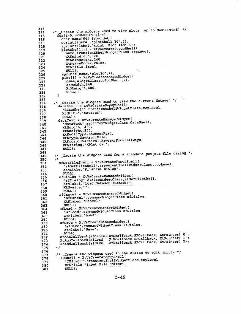
313
314
315
316
317
318
319
320
321
322
323
324
325
326
327
328
329
330
331
332
333
334
335
336
337
338
339
340
341
342
343
344
345
346
347
348
349
350
351
352
353
354
355
356
357
358
359
360
361
362
363
364
365
366
367
368
369
370
371
372
373
374
375
376
377
378
379
380
381
/* _Create the widgets used to view plots (up to MAXPLOTS=8) */
for(i=0;i<MAXPLOTS;i++) {
char name[64],label[64J;
sprintf(name ,'plotShell_%d',i);
sprintf(label,'xplot: Plot #%d',i);
plotShell[i] = XtVaCreatePopupShell(
name,transientShellWidgetClass,topLevel,
XtNminWidth, 320,
XtNminHeight,240,
XtNsaveUnder,False,
XtNtitle, label,
NULL); " - - -
sprintf(name,'plot%d',i);
plot[i] = XtVaCreateManagedWidget(
name,widgetClass,plotShell[i],
XtNwidth, 640,
XtNheight,480,
NULL);)
/* _Create the widgets used to view the current dataset */
dataShell = XtVaCreatePopupShell(
.dataShell',transientShellWidgetClass,topLevel,
XtNtitle,'Dataset',
NULL);
dataText = XtVaCreateManagedWidget(
"dataText',asciiTextWidgetClass,dataShell,
XtNwidth, 480,
XtNheight,240,
XtNeditType,XawtextRead,
XtNtype,XawAsciiFile,
XtNscrollVertical,XawtextScrollAlways,
XtNstring,'XPlot.dat',
NULL);
/* --Create the widgets used for a standard getiPut file dialog */
/*sfGetFileShell = XtVaCreatePopupShell(
"sfGetFileShell',transientShellWidgetClass,topLevel,
XtNtitle,'Filename Dialog',
NULL);
sfDialog = XtVaCreateManagedWidget(
"sfDialog',dialogWidgetClass,sfGetFileShell,
XtNlabel,'Load Dataset (Named):',
XtNvalue,'',
NULL);
sfCancel = XtVaCreateManagedWidget(
"sfCancel',con_nandWidgetClass,sfDialog,
XtNlabel,'Cancel',
NULL);
sfLoad = XtVaCreateManagedWidget(
"sfLoad',commandWidgetClass,sfDialog,
XtNlabel,'Load',
NULL);
sfSave = XtVaCreateManagedWidget(
"sfSave',commandWidgetClass,sfDialog,
XtNlabel,'Save',
NULL);
XtAddCallback(sfCancel,XtNcallback,SFCallback,(XtPointer) 0);
XtAddCallback(sfLoad ,XtNcallback, SFCallback,(XtPointer) i);
XtAddCallback(sfSave ,XtNcallback,SFCallback,(XtPointer) 2);
*/
/* _Create the widgets used in the dialog to edit inputs */
IEShell = XtVaCreatePopupShell(
"IEShell',transientShellWidgetClass,topLevel,
XtNtitle,'Input File Editor',
NULL); ........
C-49

382
383
384
385
386
387
388
389
390
391
392
393
394
395
396
397
398
399
40O
401
402
403
404
405
406
407
408
409
410
411
412
413
414
415
416
417
418
419
420
421
422
423
424
425
426
427
428
429
430
431
432
433
434
435
436
437
438
439
440
441
442
443
444
445
446
447
448
449
450
IEForm = XtVaCreateManagedWidget(
"IEForm',formWidgetClass,IEShell,
NULL);
for (i=0;i<8;i++) {
sprintf(s,'IEBox_%d',i);
IEBox[i] = XtVaCreateManagedWidget(
s,boxWidgetClass,IEForm,
XtNhSpace,1,
XtNvSpace,l,
XtNorientation,XtorientHorizontal,
NULL);
sprintf(s,'IETop_%d',i);
IETop[i] = XtVaCreateManagedWidget( _
s,labelWidgetClass,IEBox[i],
XtNresize,False,
NULL);
}for (i=0;i<6;i++) (
sprintf(s,'IEItem_%d_0",i);
if ((i<3) II (i==5))
IEItem(i][0] - XtVaCreateManagedWidget(
s,asciiTextWidgetClass,IEBox[i],
XtNdisplayCaret,False,
NULL);
else
IEItem[i][0] = XtVaCreateManagedWidget(
s,asciiTextWidgetClass,IEBox[i],
XtNeditType,XawtextEdit,
NULL);
)for (i=0;i<6;i++) {
sprintf(s,'IEItem_6_%d',i);
IEItem[6][i] = XtVaCreateManagedWidget(
s,commandWidgetClass,IEBox[6],
NULL);
XtAddCallback(IEItem[6][i],XtNcallback, IECallback,(XtPointer)
)
IEViewport = XtVaCreateManagedWidget(
"IEViewport',viewportWidgetClass,IEBox[7],
XtNallowVert,True,
XtNforceBars,True,
XtNtop,XtChainTop,XtNfromHoriz,IEBox[0],
NULL);
IEList = XtVaCreateManagedWidget(
"IEList',listWidgetClass,IEViewport,
XtNverticalList,True,
XtNcolumnSpacing,0,
XtNrowSpacing,2,
XtNdefaultColumns,l,
XtNforceColumns,True,
XtNlist,IEentries,
NULL);
XtAddCallback(IEList,XtNcallback,IEListCallback,0);
i);
XtVaSetValues(IEBox[0],XtNleft,XtChainLeft,XtNtop,XtChainTop,NULL);
for (i=l;i<7;i++)
XtVaSetValues(IEBox[i],XtNfromVert,IEBox[i-l],
XtNleft,XtChainLeft,NULL);
XtVaSetValues(IEBox[7],XtNfromHoriz,IEBox[0],XtNtop,XtChainTop,
XtNorientation,XtorientVertical,NULL);
/* _Create the widgets used in the dialog for the colors and hashes */
DAShell = XtVaCreatePopupShell(
"DAShell',transientShellWidgetClass,topLevel,
C-50

451
452
453
454
455
456
457
458
459
460
461
462
463
464
465
466
467
468
469
470
471
472
473
474
475
476
477
478
479
48O
481
482
483
484
485
486
487
488
489
490
491
492
493
494
495
496
497
498
499
50O
501
502
503
504
505
506
507
508
509
510
511
512
513
514
515
516
517
518
519
XtNtitle,'Data Attributes Editor',
NULL);
DAForm = XtVaCreateManagedWidget(
"DAForm'.formWidgetClass,DAShell,
NULL);
/.
DALabel[0] = XtVaCreateManagedWidget(
"DALabel_0",labelWidgetClass,DAForm,
XtNfromHoriz,DABox[0],
NULL);
DALabel[l] = XtVaCreateManagedWidget(
"DALabel_l', labelWidgetClass. DAForm,
XtNfromHoriz, DALabel [0 ] ,
NULL) ;
*/
for (i=0;i<5;i++) {
sprintf(s,'DABox_%d',i_;
DABox[i] = XtVaCreateManagedWidget(
s,boxWidgetClass,DAForm,
XtNhSpace, l,
XtNvSpace,l,
XtNorientation,XtorlentVertical,
XtNtop,XtChainTop.
NULL);
sprintf(s,'DATop_%d',i);
DATop[i] = XtVaCreateManagedWidget(
s,labelWidgetClass,DABox[i],
XtNresize,False,
NULL);
)for (i=l;i<5;i++)
XtVaSetValues(DABox[i].XtNfromHoriz,DABox[i-l],NULL);
for (i=0;i<16;i++) (
sprintf(s,'DAItem_0_%02d',i);
DAItem[0][i] = XtVaCreateManagedWidget(
s,labelWidgetClass,DABox[0],
XtNresize,False,
XtNlabel," ",
NULL);
)for (j=l;j<5;j++)
for (i=0;i<16;i++) (
sprintf(s.'DAItem_%d_%02d',j,i);
DAItem[j)[i] = XtVaCreateManagedWidget(
s,asciiTextWidgetClass,DABox[j],
XtNeditType,XawtextEdit,
NULL);
}
/* _Create the widgets used in the dialog to edit formats */
FEShell = XtVaCreatePopupShell(
"FEShell',transientShellWidgetClass,topLevel,
XtNtitle,'Format Editor',
NULL); - - -
FEForm = XtVaCrea£eManagedWidget(
"FEForm',formWidgetClass,FEShell,
NULL);
for (i=0;i<10;i++) {
sprintf(s.'FEBox_%d'.i);
FEBox[i] = XtVaCreateManagedWidget(
s,boxWidgetClass,FEForm.
XtNhSpace,l,
XtNvSpace,l,
NULL);
sprintf(s.'FETop_%d',i);
FETop[i] = XtVaCreateManagedWidget(
C-51

520521522523524525526527528529530531532533
534535
53653753853954054154254354454554654754854955055155255355455555655755855956056156256356456556656756856957O571572573574575576577578579580581582583584585586
587588
s,labelWidgetClass,FEBox[i],XtNresize,False,NULL);
)
XtVaSetValues(FEBox[9],XtNleft,XtChainLeft,XtNtop,XtChainTop,XtNorientation,XtorlentHorizontal,NULL);
XtVaSetValues(FEBox[0],XtNleft,XtChainLeft,XtNfrQmVert,FEBox[9],XtNorientation,XtorientHorizontal,NULL);
XtVaSetValues(FEBox[l],XtNleft,XtChainLeft,NULL);XtVaSetValues(FEBox[5],XtNleft,XtChainLeft,NULL);for (i=l;i<5;i++)
XtVaSetValues(FEBox[i],XtNfromVert,FEBox[0],
XtNfromHoriz,FEBox[i-l],NULL);
for (i=5;i<9;i++)XtVaSetValues(FEBox[i],XtNfromVert,FEBox[l],
XtNfromHoriz,FEBox[i-l],NULL);XtVaSetValues(FEBox[1],XtNfromHoriz,NULL,NULL);
XtVaSetValues(FEBox[5],XtNfromHoriz,NULL,NULL);
FEItem[9] [0] = XtVaCreateManagedWidget(
"FEItem_9_0",asciiTextWidgetClass,FEBox[9],XtNeditType,XawtextEdit,NULL);
FEItem[0][0] = XtVaCreateManagedWidget("FEItem_0_0",asciiTextWidgetClass,FEBox[0],XtNeditType,XawtextEdit,NULL);
for (i=0;i<8;i++) (sprintf(s,'FEItem_l_%d',i);FEItem[l][i] = XtVaCreateManagedWidget(
s,toggleWidgetClass,FEBox[l],XtNresize,False,XtNsensitive,False,XtNlabel,'',NULL);
}for (i=0;i<8;i++) {
sprintf(s,'FEItem_2_%d',i);FEItem[2] [i] = XtVaCreateManagedWidget(
s,toggleWidgetClass,FEBox[2],XtNresize,False,XtNsensitive,False,XtNlabel,'',NULL);
)for (i=0;i<8;i++) {
sprintf(s,'FEItem_3 %d',i);FEItem[3][i] = XtVaCreateManagedWidget(
s,toggleWidgetClass,FEBox[3],XtNresize,False,NULL);
}for (i=0;i<2;i++) {
sprintf(s,'FEItem_4_%d',i);FEItem[4][i] = XtVaCreateManagedWidget(
s,commandWidgetClass,FEBox[4],NULL);
XtAddCallback(FEItem[4][i],XtNcallback,FEPageCallback, (XtPointer)}for (i=0;i<7;i++) (
sprintf(s,°FEItem_5_%d',i);FEItem[5][i] - XtVaCreateManagedWidget( ........
s,labelWidgetClass,FEBox[5],XtNjustify,XtJustifyRight, _ _NULL);
)for (i=0;i<7;i++) {
i);
C-52

589
590
591
592
593
594
595
596
597
598
599
600
601
602
603
604
605
606
607
608
609
610
611
612
613
614
615
616
617
618
619
620
621
622
623
624
625
626
627
628
629
630
631
632
633
634
635
636
637
638
639
640
641
642
643
644
645
646
647
648
649
650
651
652
653
654
655
656
657
/*
*/
sprintf(s°'FEItem_6 %d',i);
FEItem[6] [i] = XtVaCreateManagedWidget(
s,asciiTextWidgetClass. FEBox[6],
XtNeditType,XawtextEdit,
NULL);
}for (i=0;i<7;i++) [
sprintf(s,'FEItem_7_%d',i);
FEItem[7] [i] = XtVaCreateManagedWidget(
s,asciiTextWidgetClass,FEBox[7],
XtNeditType,XawtextEdit,
NULL); _-
]
FEItem[8][0] = XtVaCreateManagedWidget(
•FEItem 8_0",asciiTextWidgetClass,FEBox[8],
XtNeditType,XawtextEdit,
NULL);
for (i=l;i<6;i++) (
sprintf(s,'FEItem_8_%d',i};
FEItem[8][i] = XtVaCreateManagedWidget(
s,commandWidgetClass,FEBox[8],
NULL);
XtAddCallback(FEItem[8][i],XtNcailback,
FECommandCallback,(XtPointer) i);
}
/* _Create the wldgets that I need to make the active plot dialog */
PMShell = XtVaCreatePopupShell (
•PMShel i", transientShellWidgetClass, topLevel,
XtNtitle,'Plot Manager',
NULL) ;
PMForm _ XtVaCreateManagedWidget(
'PMForm", formWidgetClass, PMShell,
NULL) ; .....
for (i=0;i<4;i++) {
sprintf (s, "PMBox_%d", i) ;
PMBox[i] = XtVaCreateManagedWidget
s, boxWidgetClass, PMForm,
XtNhSpace, i,
XtNvSpace, I,
XtNt op, XtChainTop,
NULL) ; - - -- -
sprintf (s, "PMTop_%d", i) ;
PMTop [i] = XtVaCreateManagedWidget (
s, labelWidgetClass, PMBox [ i ],
NULL) ; ....
XtVaSetValues (PMBox [0 ], XtNleft, XtChainLeft, NULL) ;
for (i=l; i<4; i++)
XtVaSetValues (PMBox [i ], XtNfromHoriz, PMBox [i - 1 ], NULL) ;
for (i=0;i<8;i++) {
sprintf(s,'PMToggle %d',i);
sprintf(t,'Plot #%d',i);
PMitem[0][i] = XtVaCreateManagedWidget(
s,toggleWidgetClass,PMBox[0],
XtNsensitive,False,
XtNradioData,(caddr_t) i+l,
XtNradioGroup,PMitem[0][0],
XtNlabel,t,
NULL);
XtAddCallback(PMitem[0][i],XtNcallback,
PMActiveCallback,(XtPolnter) i);
if (i!=0)
XawToggleChangeRadioGroup(PMitem[O][i_,PMitem[01[O]);
} - _
C-53
658659660661662663664665666667668669670671672673674675676677678679680
6816826836846856866876886896906916926936946956966976986997007017027037047O5706707708709710711712713714715716717718719720721722723724
725726
for (i=0;i<8;i++) {
PMitem[l][i] = XtVaCreateManagedWidget("entry',commandWidgetClass,PMBox[l],XtNresize,False,XtNsensitive. False,XtNlabel,'Create',NULL);XtAddCallback(PMitem[l][i],XtNcallback,
PMCreateCallback,(XtPointer) i);
)for (i=0;i<8;i++) (
PMitem[2] [i] = XtVaCreateManagedWidget("entry',commandWidgetClass,PMBox[2],XtNsensitive,False,XtNresize,False,XtNlabel,'Show',NULL);
XtAddCallback(PMitem[2][i],XtNcallback,PMShowHideCallback,(XtPointer) i);
)for (i=0;i<l;i++) {
sprintf(s,'PMitem_3_%d',i);PMitem[3][i] = XtVaCreateManagedWidget(
s,co_hmandWidgetClass,PMBox[3],XtNresize,False,NULL);
XtAddCallback(PMitem[3][i],XtNcallback, PMPlanarCallback, 0);
)for (i=l;i<7;i++) (
sprintf(s,'PMitem_3_%d',i);PMitem[3][i] = XtVaCreateManagedWidget(
s,commandWidgetClass,PMBox[3],XtNresize,False,NULL);
XtAddCallback(PMitem[3][i],XtNcallback,PMActionCallback,(XtPointer) i);
)
execShell = XtVaCreatePopupShell("execShell',transientShellWidgetClass,topLevel,XtNtitle,'Execution Summary',NULL);
execForm = XtVaCreateManagedWidget("execForm',formWidgetClass,execShell,NULL);
for (i=0;i<3;i++) {sprintf(s,'execBox_%d',i);execBox[i] = XtVaCreateManagedWidget(
s,boxWidgetClass,execForm,XtNhSpace,l,XtNvSpace,l,XtNtop,XtChainTop,NULL);
sprintf(s,'execTop_%d',i);execTop[i] = XtVaCreaseManagedWidget(
s,labelWidgetClass,execBox[i],NULL);
]for (i=l;i<3;i÷+)
XtVaSetValues(execBox[i],XtNfrOmHoriz,execBox[i-l],NULL);
for (i=0;i<4;i++) {
sprintf(s,'execItem_0_%d',i); ....execItem[0][i] = XtVaCreateManagedWidget(
s,labelWidgetClass,execBox[0],XtNresize,False,XtNjustify,XtJustifyRight,NULL);
C-54

727
728
729
730
731
732
733
734
735
736
737
738
739
740
741
742
743
744
745
746
747
748
749
75O
751
752
753
754
755
756
757
758
759
760
761
762
763
764
765
766
767
768
769
770
771
772
773
774
775
776
777
778
779
780
781
782
783
784
785
786
787
788
789
790
791
792
793
794
795
)for (i=0;i<4;i++) {
sprintf(s,'execItem__l_%d',i);
execltem[l] [i] = XtVaCreateManagedWidget(
s,asciiTextWidgetClass,execBox[l],
XtNeditType,XawtextEdit,
NULL);
)for (i=0;i<3;i++) {
sprintf(s,'execltem_2_%d',i);
execItem[2] [i] = XtVaCreateManagedWidget(
s,commandWidgetClass.execBox[2],
XtNresize,False,
XtNjustify,XtJustifyCenter,
NULL);
XtAddCallback(execItem[2][i],XtNcallback,ExecCallback,(XtPointer) i);
}
fileShell = XtVaCreatePopupShell(
.fileShell',translentShellWidgetClass,topLevel,
XtNtitle,'Input Data',
NULL);
filePane = XtVaCreateManagedWidget(
"filePane',panedWidgetClass,fileShell,
NULL);
fileMenuPane = XtVaCreateManagedWidget(
,fileMenuPane',panedWidgetClass, filePane,
XtNorientation,XtorientHorizontal,
XtNshowGrip,False,
XtNskipAdjust,True,
NULL);
fileEntry[0] = XtVaCreateManagedWidget{
-fileEntry_0",commandWidgetC1ass,fileMenuPane,
XtNlabel,'Done',
XtNshowGrip,False,
NULL);
fileEntry[l] = XtVaCreateManagedWidget(
"fileEntryl'.commandWidgetClass,fileMenuPane,
XtNlabel,'Save',
XtNshowGrip,False,
NULL);
fileEntry[2] = XtVaCreateManagedWidget(
"fileEntry2",commandWidgetClass,fileMenuPane,
XtNlabel,'Load',
XtNshowGrip,False,
NULL);
for (i=0;i<3;i÷+)
XtAddCallback(fileEntry[i],XtNcallback,FileCallback,(XtPointer) i);
fileEntry[3] = XtVaCreateManagedWidget(
"fileEntry 3".asciiTextWidgetClass,fileMenuPane.
XtNeditType,XawtextEdit,
XtNshowGrip,False,
NULL);fileText = XtVaCreateManagedWidget(
"fileText',asciiTextWidgetClass,filePane,
XtNwidth, 480,
XtNheight, 240,
XtNeditType,XawtextEdit,
XtNscrollVertical,XawtextScrollAlways,
XtNshowGrip. False,
NULL);
/* Create the widgets for the motor geometry dialog */
MGShell = XtVaCreatePopupShell(
°MGShell',transientShellWidgetClass,topLevel,
XtNtitle,'Solid Rocket Motor Geometry'.
NULL);
MGForm = XtVaCreateManagedWidget(
C-55

796
797
798
799
800801
802
803
804
805
806
807
808809
810
811
812
813
814
815
816
817
818
819
820
821
822
823
824
825
826
827
828
829
830
831
832
833
834
835
836
837
838
839
840
841
842
843
844
845
846
847
848849
850851852853854855856
857
858
859
86O
861
862
863
864
,MGForm',formWidgetClass,MGShell,
NULL);
for (i=0;i<6;i++) (
sprintf(s,'MGBox_%d',i);
MGBox[i] = XtVaCreateMaI%agedWidget(
s,boxWidgetClass,MGForm,
XtNhSpace,l,
XtNvSpace,l,
NULL);
sprintf(s,'MGTop_%d',i);
MGTop[i] = XtVaCreateManagedWidget(
s,labelWidgetClass,MGBox[i],
NULL);
}XtVaSetValues(MGBox[O],XtNleft,XtChainLeft,XtNtop,X_ChainTop,NULL);
for (i=l;i<3;i++)
XtVaSetValues(MGBox[i],XtNfromHoriz,MGBox[i-l],NULL);
XtVaSetValues(MGBox[3],XtNfromVert,MGBox[0],XtNleft,XtChainLeft,NULL);
for (i=4;i<6;i++)
XtVaSetValues(MGBox[i],XtNfromHoriz,MGBox[il],
XtNfromVert,MGBox[0],NULL);
MGPictShell = XtVaCreatePopupShell(
,MGPictShell,,transientShellWidgetClass,topLevel,
XtNminWidth,240,
XtNminHeight,240,
XtNmaxAspectX, l,
XtNmaxAspectY,l,
XtNsaveUnder,False,
XtNtitle,'XXX',
NULL);
MGPict = XtVaCreateManagedWidget(
,MGPict',widgetClass,MGPictShell,
XtNwidth,360,
XtNheight,360,
NULL);
for (i=0;i<8;i++) {
sprintf(s,'MGItem_0_%d',i);
MGItem[0][i] = XtVaCreateManagedWidget(
s,labelWidgetClass,MGBox[0],
XtNresize,False,NULL);
)for (i=0;i<8;i++) {
sprintf(s,'MGItem_l_%d',i);
MGItem[l][i] = XtVaCreateManagedWidget(
s,asciiTextWidgetClass,MGBox[l],
XtNeditType,XawtextEdit,NULL);
)for (i=0;i<6;i++) {
sprintf(s,'MGItem_2_%d',i);
MGItem[2][i] = XtVaCreateManagedWidget(
s,toggleWidgetClass,MGBox[2],
XtNradioGroup,MGItem[2] [0],
XtNradioData,(caddr_t) i+l,
XtNresize,False,NULL);
)XtVaSetValues(MGItem[2] [0],XtNstate,True,NULL);
for (i=0;i<2;i++) (
sprintf(s,'MGItem_3_%d',i);
MGItem[3][i] = XtVaCreateManagedWidget(
s,labelWidgetClass,MGBox[3],
XtNresize,False,NULL);
}for (i=0;i<2;i++) { _ _
sprintf(s,'MGItem_4_%d',i);
MGItem[4][i] = XtVaCreateManagedWidget(
s,asciiTextWidgetClass,MGBox[4],
XtNeditType,XawtextEdit,NULL);
C-56

865
866
867
868
869
870
871
872
873
874
875
876
877
878
879
880
881
882
883
884
885
886
887
888
889
89O
891
892
893
894
895
896
897
898
899
900
901
902
903
904
905
906
907
908
909
910
911
912
913
914
915
916
917
918
919
)
for (i=0;i<4;i++) {
sprintf(s,'MGItem_5_%d',i);
MGItem[5] [i] = XtVaCreateManagedWidget(
s,commandWidgetClass,MGBox[5],NULL);
XtAddCallback(MGItem[5] [i],XtNcallback,MGCallback,(XtPointer)
)
/* Create the widgets for the curve fitting dialog */
CFShell = XtVaCreatePopupShell(
"CFShell',transientShellWidgetClass,topLevel,
XtNtitle,'Data Curve Fitting',
NULL);
CFForm = XtVaCreateManagedWidget(
°CFForm',formWidgetClass,CFShell,
NULL);
for (i=0;i<3;i++) {
sprintf(s,'CFBox_%d',i);
CFBox[i] = XtVaCreateManagedWidget(
s,boxWidgetClass,CFForm,
XtNhSpace,l,
XtNvSpace,l,
XtNtop,XtChainTop,
NULL);
sprintf(s,'CFTop_%d',i);
CFTop[i] = XtVaCreateManagedWidget(
s,labelWidgetClass,CFBox[i],
NULL);
)
for (i=l;i<3;i++)
XtVaSetValues(CFBox[i],XtNfromHoriz,CFBox[i-l],NULL);
for (i=0;i<16_i++) {
sprintf(s,'CFItem_0_%d',i);
CFItem[0][i] = XtVaCreateManagedWidget(
s,toggleWidgetClass,CFBox[0],
XtNlabel,'',
XtNresize,False,
XtNaensitive,False,NULL);
)
for (i=0;i<16;i++) (
sprintf(s,'CFItem_1%d',i);
CFItem[l][i] = XtVaCreateManagedWidget(
s,asciiTextWidgetClass,CFBox[l],
XtNeditType,XawtextEdit,NULL);
)
for (i=0;i<4;i++) (
sprintf(s,'CFItem_2 %d',i);
CFItem[2] [i] = XtVaCreateManagedWidget(
s,commandWidgetClass,CFBox[2],
NULL);
)
}
i);
C-57

Related Documents