NASA Contractor Report 189618 qS · assessment, and Alan K. Mortlock, technical assessment. Other Douglas staff that made essential contributions to the HSCT team contract work included:

NASA Contractor Report 189618

/H --.,:::J<G.....

qS/ _/'_-j. <.':;>.,?

1990 High-Speed Civil Transport Studies

HSCT Concept Development Group

Advanced Commercial Programs

McDonnell Douglas Corporatlon

Douglas Aircraft Company

Long Beach, Callfornla

Contract NAS I - 18378

October 1992 (NASA-CR-189618) THE 1990

HIGH-SPEED CIVIL TRANSPORT STUOIES

Final Report, 1 Oct. 1989 - 31 Mar.

1991 (McDonnell-Douglas Corp.)75 p

NASANational Aeronautics andSpace Administration

Langley Research CenterHampton, Virginia 23665-5225

G3/05

N93-16947

Unclas

0127091

https://ntrs.nasa.gov/search.jsp?R=19930007758 2020-05-27T03:27:33+00:00Z

REPORT MDC K0395-2

1990 HIGH-SPEEDCIVIL TRANSPORT STUDIES

HSCT CONCEPT DEVELOPMENT GROUPADVANCED COMMERCIAL PROGRAMS

DOUGLAS AIRCRAFT COMPANYLONG BEACH, CA 90846

CONTRACT NAS1-18378

ABSTRACT

This report contains the results of the Douglas Aircraft Company system studies related to

high-speed civil transports (HSCTs). The tasks were performed under an 18-month extension

of NASA Langley Research Center Contract NAS1-18378.

The system studies were conducted to assess the emission impact of HSCTs at design Mach

numbers ranging from 1.6 to 3.2. The tasks specifically addressed an HSCT market and eco-

nomic assessment, development of supersonic route networks, and an atmospheric emissions

scenario.

The general results indicated (1) market projections predict sufficient passenger traffic forthe 2000 to 2025 time period to support a fleet of economically viable and environmentally

compatible HSCTs; (2) the HSCT route structure to minimize supersonic overland traffic can

be increased by innovative routing to avoid land masses; and (3) the atmospheric emission

impact on ozone would be significantly lower for Mach 1.6 operations than for Math 3.2

operations.

iii

PRECEDING P++-_t_.+_._.+A,NK NO'_" FUL_D

t

FOREWORD

The 1990 High-Speed Civil Transport Study was an 18-month extension of the previous3 years' work (Phases I to IliA). The 1990 systems studies evaluation covered the period from1 October 1989 to 31 March 1991.

Work was accomplished as a task order activity by Douglas Aircraft Company in Long Beach,

California. This work was under the direction of the NASA Langley Research Center, Hamp-ton, Virginia, and was funded under Contract NAS1-18378.

The NASA Contracting Officer Technical Representative was Donald U Maiden. The Doug-las program manager was initially Donald A. Graf, HSCT business unit manager, and, in thelatter 9 months of the contract, Bruce L Bun/n, business unit manager-Advanced Commer-

cial Programs. Principal investigators were Munir Metwally, market research and economicassessment, and Alan K. Mortlock, technical assessment.

Other Douglas staff that made essential contributions to the HSCT team contract workincluded:

Administration Elaine Anderson

Aerodynamics John Morgenstern, Roland Schmid, C. J. Turner

Business Operations Melanie Shell

Contract Support Joan Ferri

Marketing Research Harry Landau, Rod Weissler

Propulsion Gordon Hamilton, Tony Velleca, Ken Williams

_ 0__ _ _i,A__

CONTENTS

Section Page

1

2

3

SUMMARY ................................................ 1

INTRODUCTION .......................................... 3

MARKET AND ECONOMIC ASSESSMENT ................... 5

Traffic Projection ...................................... 53.1

3.2

3.3

Fleet

Cash

3.3.1

3.3.2

3.3.3

3.3.4

3.3.5

Requirement ..................................... 8

Operating Cost Comparison ......................... 13Revenue ....................................... 13

Operating Costs ................................ 13

Operating Profit ................................ 14Aircraft Worth .................................. 15

Conclusion and Further Studies. ...... ............. 15

4 SUPERSONIC NETWORK EVALUATION ..................... 17

4.1 Aircraft Economic Performance .......................... 18

4.1.1 Time Savings ................................... 18

4.1.2 Operating Cost and Profit ........................ 184.1.3 Aircraft Worth .................................. 19

4.1.4 Fare Premium .................................. 21

4.2 Supersonic Network Scenarios ............................ 22

4.2.1 Methodology ................................... 22

4.2.2 Route Diversion Analysis ......................... 24

4.2.3 Overwater Network Scenario ...................... 27

4.3 Conclusion ........................................... 28

4.4 Recommendations for Further Study ...................... 28

5 ATMOSPHEIRC EMISSIONS IMPACT STATUS ................. 33

5.1 Brief Methodology Review .............................. 33

5.2 Atmospheric Emission Scenarios .......................... 34

5.3 Ozone Impact Trade Studies ............................. 365.4 Cruise Altitude Restrictions .............................. 39

5.5 Conclusions ........................................... 44

5.6 Future Plans and Recommendations ..... • ................. 45

6 CONCLUSIONS ............................................ 47

7 RECOMMENDATIONS ..................................... 49

APPENDIX A -- Basic Traffic Data Base, 250 City-Pairs in

Descending Order of Scheduled Seats ...................... A-1

APPENDIX B -- Great Circle Versus Diverted Distances, Strip

Charts for Top 20 City-Pairs ............................... B-1

APPENDIX C -- Ground Track Profile Display, 250 City-Pairs., ............... C-1

vii

Figure

3-1

3-2

3-3

3-4

3-5

3-6

3-7

3-8

3-9

3-10

3-11

3-12

3-13

4-1

4-2

4-3

4-4

4-5

4-6

4-7

4-8

4-9

4-10

4-11

4-12

4-13

4-14

4-15

5-1

5-2

5-3

5-4

ILLUSTRATIONS

Page

Douglas Mach 1.6 Turbulent Baseline Configuration, D1.6-3 ......... 6

Douglas Mach 2.2 Turbulent Baseline Configuration, D2.2-10 ........ 6

Douglas Mach 3.2 Turbulent Baseline Configuration, D3.2-7A ........ 7

International Passenger Traffic -- Major Regions

(85-90 Percent of Total) ...................................... 7Distribution of Annual Seat-Miles for Major 10 Regions

for Year 2000 .............................................. 8

Passenger Aircraft Capacity/Supply Forecast ....................... 9

Passenger Capacity Trends by Generic Class 9

Commercial Passenger Jetliners in Year 2000 ...................... 10

Generic Passenger Aircraft Requirements in Year 2000 .............. 11

Generic Passenger Aircraft Requirements IncludingSupersonic Class in Year 2000 ................................. 11

Projected HSCT Demand in Year 2000 as a Functionof Fare Premium Levels • 12

Operating Cost Breakdown -- No Ownership-Related Costs .......... 14

Operating Performance (Revenue - Cost = Profit) ................. 15

Time Performance ............................................ 18

Operating Performance ........................................ 19

Economic Performance Percentage of Operating Costand Profit to Revenue ....................................... 20

HSCT Miles per 1,000 Pounds of Fuel at 4,500 n mi ................ 20

Effect of Overland Off-Design Operation on Aircraft Worth .......... 21

Time Savings and Trip Price Relationship ......................... 22

Supersonic Network Scenarios for Unrestricted andRestricted Operation ........................................ 23

'fi'affic Analysis by IATA Regions ................................ 23

Top 250 Potential Supersonic Routes (No Restrictions) .............. 25

City-Pair Evaluation -- JFK (New York)-LHR (London) ............. 26

Diverted Routing -- New York-Tokyo ............................ 27

HSCT Top Seat Rank 250 Airport-Pairs ........................... 29

HSCT Top Seat Rank 150 Airport-Pairs ........................... 30

100 City-Pairs for Overwater Only -- Supersonic Network ........... 31

Supersonic Network Scenario for 200 City-Pairs ................... 32

HSCT Representative City-Pairs ................................. 34

Data Flow for Generating Inputs to Global Atmospheric Models ...... 35

Ozone Depletion by Year -- P&W TBE Engine .................... 37

ozone Depletion Versus Engine Type -- Mach 3.2 .................. 37t

ix _ ....._ _, _,_;i_Joi_i_!_ _ __! o

Figure

5-5

5-6

5-7

5-8

5-9

5-10

5-11

5-12

5-13

5-14

Page

Ozone Depletion and Fleet Size Versus Number of Flightsfor P&W TBE .............................................. 38

Fare Premium Impact on Ozone Concentration .................... 39

Cruise Altitude Restriction Ozone Impact ......................... 40

Effects of Cruise Altitude Restriction on MTOGW

and Range -- Math 3.2 ...................................... 41

Effect of Cruise Altitude Restriction on Market Capture42

(Annual Seat-Miles) .........................................

Effect of Cruise Altitude on Operating Performance -- Math 3.2 ..... 42

Effect of Cruise Altitude Restrictions on Operating Cost

and Profit -- Mach 3.2 ....................................... 43

Effect of Cruise Altitude Restriction on Operating Cost

and Fuel Cost -- Mach 3.2 Without Resizing .................... 43

Effect of Cruise Altitude on Aircraft Worth and Operating Profit --

Mach 3.2 Without Resizing ................................... 44

Effect of Cruise Altitude Restrictions on Aircraft Worth

After Commencement of Production (Without Resizing) ........... 45

Table

3-1

3-2

3-3

3-4

:3-5

3-6

4-I

5-I

5-2

5-3

TABLES

Page

Fleet Projections Based on HSCT Demand ........................ 12Revenue for Mach 1.6, 2.2, 3.2 Aircraft ........................... 13

Annual Revenue per Aircraft ................................... 13

Operating Cost Data for Mach 1.6, 2.2, 3.2 Aircraft ................. 14

Annual Cash Flow per Aircraft ............... , .................. 15

Aircraft Worth at 10-Percent ROI ................................ 16

Example of Ground Track Profile Display for New York-Tokyo ....... 28

Total Annual Fuel Burn by Region ............................... 36

NOx Emission Indices for Various Engine Concepts ................. 36

Aircraft Economic Performance at Different Cruise Altitudes ......... 44

xi

SECTION1SUMMARY

The 1990 system study report contains technical, environmental, marketing, and economicassessments; discusses issues and concerns; and makes recommendations for further systemstudies. This report focuses on the atmospheric emission impact, marketing, and economic

aspects of the HSCT. It contains results of a Douglas Aircraft Company study to evaluate thecommercial viability of the HSCT. The approach was to evaluate, under simulated airline

operations, worldwide market demand, fleet requirements, realistic supersonic route struc-tures, and HSCT economic performance. Subsequently, atmospheric emission scenarios were

developed, and emission impact was evaluated for three Math number configurations -- 1.6,

2.2, and 3.2.

Market and Economic Assessments -- Traffic projections for the years 2000 to 2025 and fleet

requirements over a Mach number range of 1.6 to 3.2 have been assessed with regard to Machnumber, fare premium, and aircraft range. At Mach 2.2, fleet needs could total 2,300 or more300-seat aircraft by the year 2025. The prime conditions for economic viability include (1) air-

plane revenues covering operating costs plus an attractive rate of return to the operator,(2) fares compatible with the subsonic fleet to expand HSCT service, and (3) a market largeenough to permit a selling price lower than the investment value of the airplane.

Supersonic Network Evaluation -- Only a few candidate global airline network scenarios forHSCT have been assembled. The high-density long-range markets were selected from theOfficial Airline Guide (OAG) on-line data base. Creative rerouting was conducted to mini-

mize overland segments and to lessen the impact of the environmental restrictions that may

be imposed on future supersonic operation.

The data on these network scenarios represent an assembly of global routes from which

HSCT global traffic networks can be constructed. The network scenarios provide examples

on how supersonic service may bring some changes to the current global route structure.Some of these supersonic network scenarios show good potential of capturing more than half

the market share of the long-range traffic.

Atmospheric Emissions Impact Status -- An engine emission annual fuel burn model was

developed for input to 20 atmospheric models. Atmospheric emission scenarios were pro-dueed for three HSCT configurations at Mach 1.6, 2.2, and 3.2 The atmospheric global modelresults showed that ozone depletion is a function of the aircraft's cruise Mach number pri-

marily because of the strong dependence of ozone impact on injection altitude. The atmos-pheric impact of ozone depletion of the Mach 1.6 configuration is considerably less than thatof the Math 2.2 and 3.2 configurations for a given combustor technology. The introductionof cruise altitude restrictions after the HSCT enters service could alleviate the ozone impact

of the Mach 1.6 and 2.2 configurations. At Mach 3.2, however, the increased fuel burn more

than offsets the advantage of lower injection altitude. All configurations will suffer some eco-

nomic performance penalties if forced below their optimum operating cruise altitude.

SECTION 2

INTRODUCTION

This report presents the results of Douglas HSCT system studies. It is a continuation of envi-

ronmental and economic studies completed in the 1989 system study. In this report, market

projections have been made for the years 2000 to 2025, fleet requirements have been assessedover a Mach number range of 1.6 to 3.2, and a number of supersonic network scenarios have

been evaluated.

Additionally, for atmospheric studies, engine emissions have been developed into annualemission fuel burn constituents to provide input data to an atmospheric impact two-dimen-

sional model.

r._ ' ,_ [_"f°_,_,'..':" _. '_' i_,_:-'_'_:' ,_:, '_.',-'_

SECTION 3

MARKET AND ECONOMIC ASSESSMENT

NASA Report 4235, submitted by Douglas at the conclusion of the Phase HI studies, includedan initial screening from Mach 2 to Mach 25, followed by a focus on the Mach 2 to Mach 5

range, as well as a comparison of Math 3.2 and Math 5.0. The economic potential for a

high-speed commercial transport with respect to technical readiness, market characteristics,aviation infrastructure, and environmental issues was described. A forecast of air travel pas-

sengers indicated a need for HSCT service in the 2000-2025 time frame, conditioned on eco-

nomic viability and environmental compatibility. Design requirements for this study focused

on a 300-passenger, three-class aircraft with a range of 6,500 nautical miles, based on acceler-

ated growth predictions for the Pacific region. Aircraft productivity was a key parameter, withaircraft worth in comparison to aircraft price being the airline-oriented figure of merit.

As a follow-up on previous studies, research for Task 11 has focused on three configuration

designs: Maeh 1.6, 2.2, and 3.2. An economic analysis of supersonic operation based on air-

craft spedfications has been conducted. The market research reflects refinements in market

assumptions and projections, a better understanding of market elasticity and stimulation, the

latest preliminary estimates for fleet requirements, the sensitivity of aircraft performance andeconomics to environmental constraints, and an updated parametric analysis of different

design range and passenger configurations. This section covers traffic projection, fleet assess-

ment, and an economic comparison of the three configuration designs at Math 1.6, 2.2,

and 3.2.

Three-view drawings of the baseline configurations used in the 1990 system studies for vari-

ous environmental and economic studies are shown in Figures 3-1, 3-2, and 3-3. The develop-

ment of these configurations was based on earlier phases of the current Douglas HSCT system

study contract and on the Douglas Advanced Supersonic Transport (AST) activities of the1970s. The fuselage was designed to accommodate 300 passengers in a nominal seating

arrangement of three classes: 10, 30, and 60 percent for first, business, and coach classes,

respectively. HSCT performance was analyzed according to commerdal domestic and inter-national rules and practices. The HSCT design range was 6,500 nautical miles in an all-super-

sonic cruise condition.

3.1 TRAFFIC PROJECTION

Traffic projection initially encompassed all international air traffic in 18 International Air

Transport Association (IATA) regions. The 10 regions considered to be the best potential for

supersonic operation were then studied in more detail. The air traffic forecasts prepared for

the 10 regions were based on econometric models that relate traffic to national income, fares,

yield, and, where appropriate, other relevant variables. Four of the 10 regions comprise about

85 percent of the total international traffic. Rapid economic growth in the Padfic-Asia regionhas made this the fastest growing area for passenger traffic. Figure 3-4 shows that North and

Mid-Pacific traffic will equal North Atlantic traffic by the year 2000.

Long-term prospects for international passenger traffic gains are relatively good. Overall,

traffic is predicted to total about 450 billion annual seat-miles (ASMs) by the year 2000 and

5

r

AR ,, 2.3LE SWEEP - 61 DEG

163 FT 7 IN.

.y.,,, .7._----=

FIGURE 3.-1. DOUGLAS MACH 1.6 TURBULENT BASELINE CONFIGURATION, D1.6-3

AR - 1.84LE SWEEP = 71/61.5 DEG

-t63FT6IN.

LRCO18-B1

FIGURE 3-2. DOUGLAS MACH 2.2 TURBULENT BASELINE CONFIGURATION, D2.2-10

J

AR 1.55

LE SWEEP -, 76/62 DEG _/ _'/')r_7: = I

FIGURE 3-3. DOUGLAS MACH 3.2 TURBULENT BASELINE CONFIGURATION, D3.2-7A

EUROPE/FAR EASTAUSTRAUA/ASIA

NORTH AND

MID-PAClFI(_ I"'_

NORTHATLANTIC

INTRA-FAR EASTAUSTRAUA

1986

EUROPE INTRA- NORTH/ NORTHFAR EAST FAR EAST MID-PACIFIC ATLANTIC

RPMs (BILLION)LRC012-157

FIGURE 3-4. INTERNATIONAL PASSENGER TRAFFIC - MAJOR REGIONS

(85-90 PERCENT OF TOTAL)

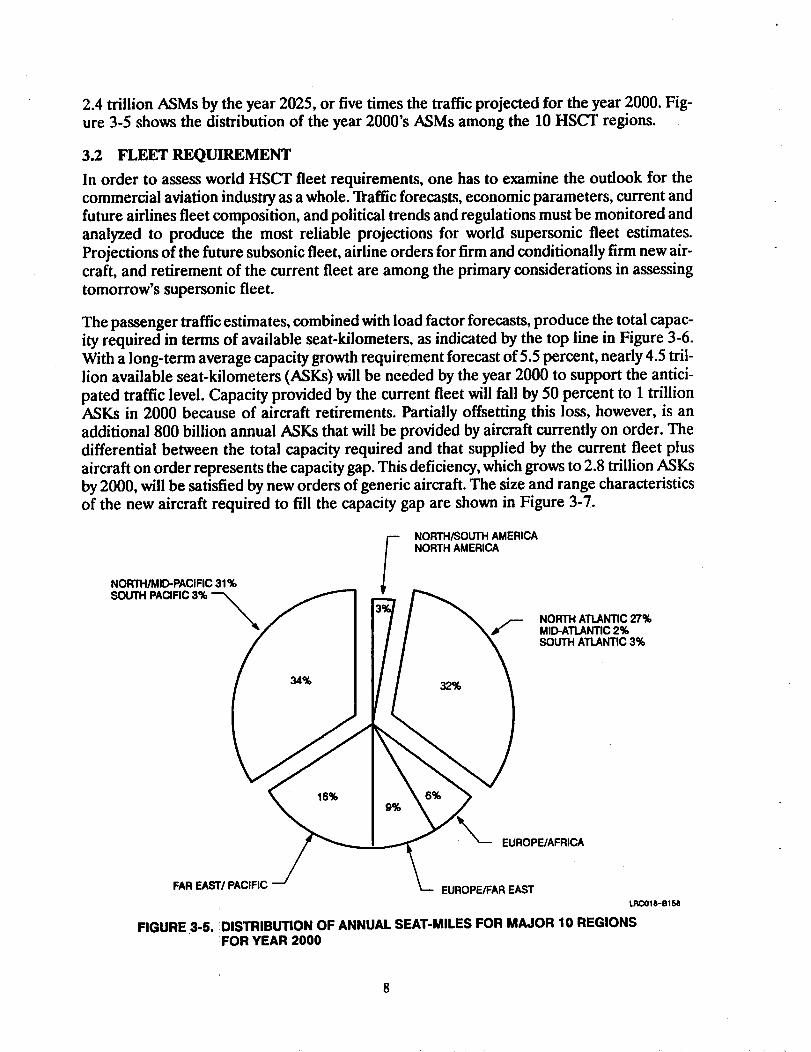
2.4 trillion ASMs by the year 2025, or five times the traffic projected for the year 2000. Fig-ure 3-5 shows the distribution of the year 2000's ASMs among the 10 HSCT regions.

3.2 FLEET REQUIREMENT

In order to assess world HSCT fleet requirements, one has to examine the outlook for the

commercial aviation industry as a whole. Traffic forecasts, economic parameters, current and

future airlines fleet composition, and political trends and regulations must be monitored and

analyzed to produce the most reliable projections for world supersonic fleet estimates.Projections of the future subsonic fleet, airline orders for firm and conditionally firm new air-craft, and retirement of the current fleet are among the primary considerations in assessingtomorrow's supersonic fleet.

The passenger traffic estimates, combined with load factor forecasts, produce the total capac-

ity required in terms of available seat-kilometers, as indicated by the top line in Figure 3-6.With a long-term average capacity growth requirement forecast of 5.5 percent, nearly 4.5 tril-

lion available seat-kilometers (ASKs) will be needed by the year 2000 to support the antici-

pated traffic level. Capacity provided by the current fleet will fall by 50 percent to 1 trillionASKs in 2000 because of aircraft retirements. Partially offsetting this loss, however, is an

additional 800 billion annual ASKs that will be provided by aircraft currently on order. Thedifferential between the total capacity required and that supplied by the current fleet plus

aircraft on order represents the capacity gap. This deficiency, which grows to 2.8 trillion ASKsby 2000, will be satisfied by new orders of generic aircraft. The size and range characteristics

of the new aircraft required to fill the capacity gap are shown in Figure 3-7.

fNORTH/MID-PACIFIC 31% J,SOUTH

NORTH/SOUTH AMERICANORTH AMERICA

NORTH ATLANTIC 27%MID-ATLANTIC 2%SOUTH ATLANTIC 3%

34% 32%

16%

EUROPE/AFRICA

FAR EAST/PACIFIC EUROPE/FAR EASTLRCOt8-B158

FIGURE 3-5. DISTRIBUTION OF ANNUAL SEAT-MILES FOR MAJOR 10 REGIONSFOR YEAR 2000

AVAILABLESEAT-

KILOMETERS(TRILLION)

4

01982

FIGURE3-6.

REOUI

ORDERS

GENERICAIRCRAFTCAPACITY

GAP

CURRENT FLEET

I I1987 1902 1997 2000

YEAR LRCmS-m_

PASSENGER AIRCRAFT CAPACITY�SUPPLY FORECAST

AVAILABLESEAT-

KILOMETERS(TRILLION)

3

LR4OO/eO0

MR-200

RR-leO

I SR-110

01982 1987 lgg2 1997 2000

YEAR _1_150

FIGURE 3-7. PASSENGER CAPACn'Y TRENDS BY GENERIC CLASS

Increased capacity will be demanded for all genetic aircraft classes. However, it is significantthat certain classes will outperform others on a relative basis. Inherent in the forecast is the

fact that both airport and airspace congestion will force carriers to rely increasingly on largeraircraft instead of increased frequencies to satisfy projected traffic demands. Airlines will also

rely on aircraft with higher productivity, such as the HSCT, to reduce congestion.

Airline transitions from subsonic aircraft to supersonic will also have an impact on the num-

ber of genetic aircraft in the medium- and long-range categories. Productivity gains necessaryto achieve the 5.5-percent worldwide average ASK escalation will be realized by changes in

four components: aircraft units, average seat counts, utilization, and speed. An increase inaircraft units will be the dominant element in increasing ASKs. As larger transports replacesmaller ones, the average seat count per aircraft will contribute to productivity gains. A rela-

tively subordinate role will be played by aircraft utilization and increased flight speed unlessthe HSCT becomes available for commercial airlines. Hscr productivity gain due to speed

will then become the dominant component, replacing aircraft units. It is conceivable that pro-

ductivity gain may ultimately cause a decline in fleet size.

The growth in the world's airline industry will necessitatechangesin the number and typeof aircraft that serve it. Overall, the 6,500 passenger aircraft operated commercially by thelate 1980s will advance to a world fleet approximating 10,000 airliners by the year 2000, a

54-percent unit increase. The dominant position of the short-range fleet will moderate as itfalls to 56 percent of the world fleet in 2000 from its present 68-percent unit share. Themedium- and long-range fleets will generate a significant relative unit gain over the forecast

period.

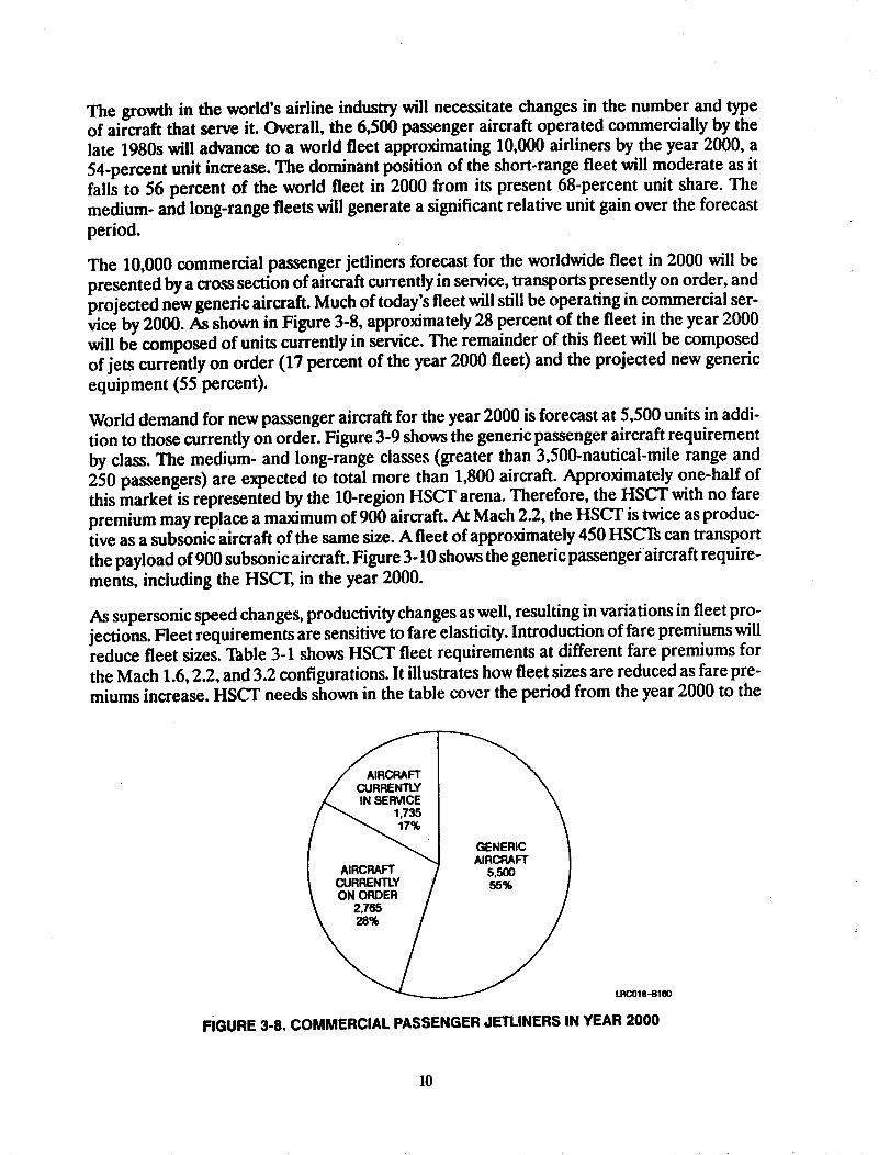
The 10,000 commercial passenger jetliners forecast for the worldwide fleet in 2000 will be

presented by a cross section of aircraft currently in service, transports presently on order, andprojected new generic aircraft. Much of today's fleet will still be operating in commercial ser-vice by 2000. As shown in Figure 3-8, approximately 28 percent of the fleet in the year 2000will be composed of units currently in service. The remainder of this fleet will be composedof jets currently on order (17 percent of the year 2000 fleet) and the projected new generic

equipment (55 percent).

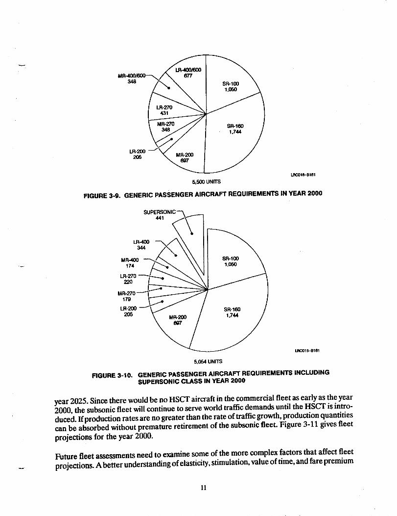
World demand for new passenger aircraft for the year 2000 is forecast at 5,500 units in addi-tion to those currently on order. Figure 3-9 shows the generic passenger aircraft requirement

by class. The medium- and long-range classes (greater than 3,500-nautical-mile range and250 passengers) are expected to total more than 1,800 aircraft. Approximately one-half ofthis market is represented by the 10-region HSCT arena. Therefore, the HSCT with no fare

premium may replace a maximum of 900 aircraft. At Mach 2.2, the HSCT is twice as produc-tive as a subsonic aircraft of the same size. A fleet of approximately 450 HSCTs can transport

the payload of 900 subsonic aircraft. Figure 3-10 shows the generic passengeraircraft require-ments, including the HSCT, in the year 2000.

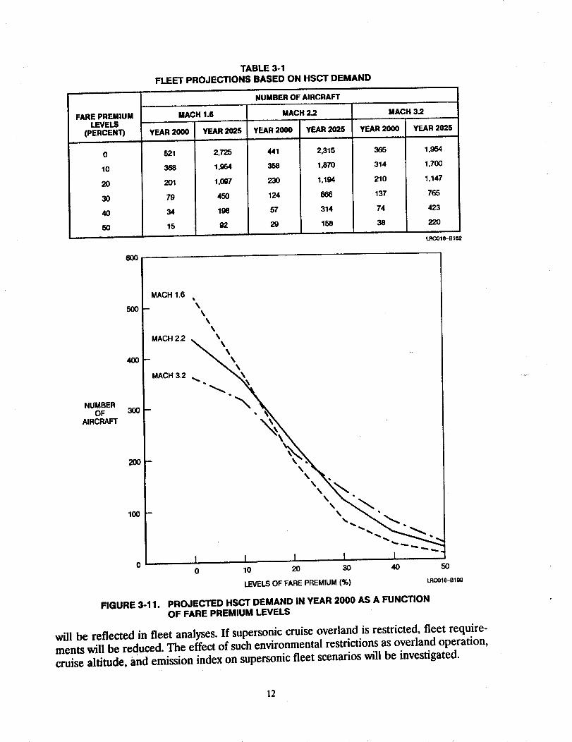
As supersonic speed changes, productivity changes as well, resulting in variations in fleet pro-jections. Fleet requirements are sensitive to fare elasticity. Introduction of fare premiums willreduce fleet sizes. Table 3-1 shows HSCT fleet requirements at different fare premiums forthe Mach 1.6, 2.2, and 3.2 configurations. It illustrates how fleet sizes are reduced as fare pre-miums increase. HSCT needs shown in the table cover the period from the year 2000 to the

/... t. SE.MCE ",/ _ 1735

/ _17%

( AI.c.An A,.C.A r I/ /

ON ORDER/J

LRCO18-B1_IO

FIGURE 3-8. COMMERCIAL PASSENGER JETLINERS IN YEAR 2000

10

LRCO18-B161

5.500 UNITS

FIGURE 3-9. GENERIC PASSENGER AIRCRAFT REQUIREMENTS IN YEAR 2000

LR-400344

MR-400174

LR-27022O

K179

LR-2002O5

FIGURE 3-10.

441

SR.-IO01,050

MR-200_7

SR-160

1.744

LRCO18-BI01

5.054UNITS

GENERIC PASSENGER AIRCRAFT REQUIREMENTS INCLUDINGSUPERSONIC CLASS IN YEAR 2000

year 2025. Since there would be no HSCT aircraft in the commercial fleet as early as the year2000, the subsonic fleet will continue to serve world traffic demands until the HSCT is intro-duced. If production rates are no greater than the rate of traffic growth, production quantitiescan be absorbed without premature retirement of the subsonic fleet. Figure 3-11 gives fleet

projections for the year 2000.

Future fleet assessments need to examine some of the more complex factors that affect fleet

projections. A better understanding of elasticity, stimulation, value of time, and fare premium

11

FARE PREMIUMLEVELS

(PERCENT)

0

10

2O

3O

4O

5O

6OO

TABLE 3-1

FLEET PROJECTIONS BASED ON HSCT DEMAND

NUMBER OF AIRCRAFT

MACH 1.6 MACH 2.2 MACH 3.2

YEAR 2000 YEAR 2025 YEAR 2000YEAR 2000

521

368

201

79

34

15

YEAR 2025

2.725

1.954

%007

45O

196

92

441

358

230

124

57

29

2,315

1,870

1.194

666

314

158

385

314

210

137

74

38

YEAR 2025

1.954

1.700

1.147

765

423

22O

LRC018-Bh,2

NUMBEROF

AIRCRAFT

5OO

4OO

3OO

20O

100

MACH 1.6

MACH 2.2

MACH 3.2

\

\

\\

\

I I I I I0 0 10 20 30 40

LEVELS OF FARE PREMtUM (%) LRCOle-mOO

FIGURE 3-11. PROJECTED HSCT DEMAND IN YEAR 2000 AS A FUNCTION

OF FARE PREMIUM LEVELS

will be reflected in fleet analyses. If supersonic cruise overland is restricted, fleet require-

ments will be reduced. The effect of such environmental restrictions as overland operation,

cruise altitude, and emission index on supersonic fleet scenarios will be investigated.

12

3.3 CASH OPERATING COST COMPARISON

For a profitable supersonic operation, the airplane must generate enough revenue to cover

its operating costs plus an attractive rate of return to the airlines. This section summarizes

the results of the cash operating cost analysis and the commercial value of the three baseline

configuration designs at Mach 3.2, 2.2, and 1.6. This evaluation examines the revenue side

of the equation, followed by the operating cost, in order to arrive at the operating profit.

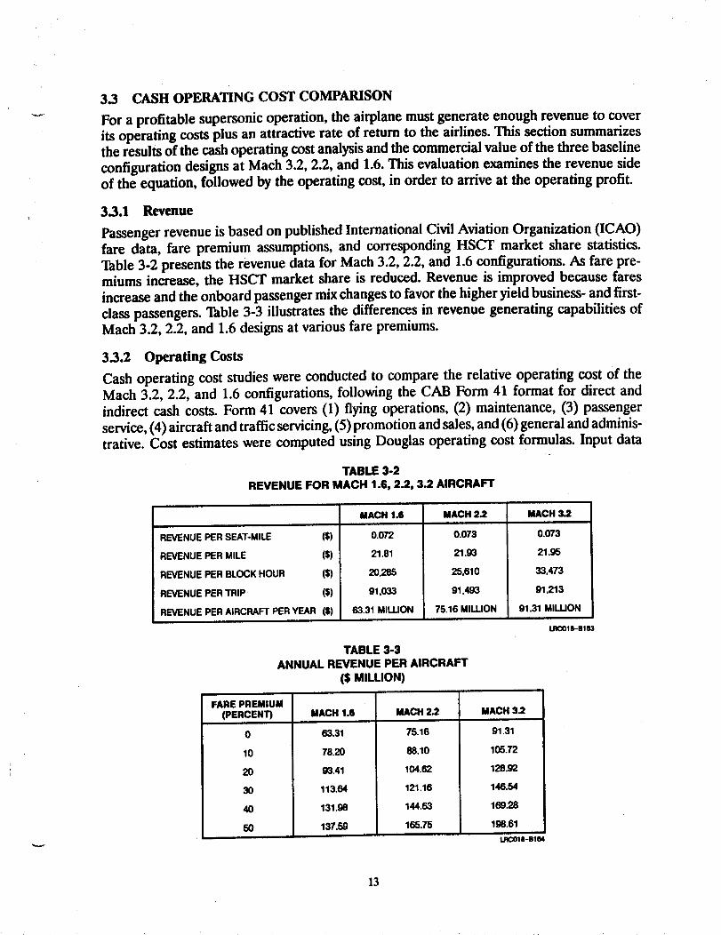
3.3.1 Revenue

Passenger revenue is based on published International Civil Aviation Organization (ICAO)

fare data, fare premium assumptions, and corresponding HSCT market share statistics.

Table 3-2 presents the revenue data for Mach 3.2, 2.2, and 1.6 configurations. As fare pre-miums increase, the HSCT market share is reduced. Revenue is improved because fares

increase and the onboard passenger mix changes to favor the higher yield business- and first-

class passengers. Table 3-3 illustrates the differences in revenue generating capabilities ofMach 3.2, 2.2, and 1.6 designs at various fare premiums.

3.3.2 Operating Costs

Cash operating cost studies were conducted to compare the relative operating cost of the

Mach 3.2, 2.2, and 1.6 configurations, following the CAB Form 41 format for direct and

indirect cash costs. Form 41 covers (1) flying operations, (2) maintenance, (3) passenger

service, (4) aircraft and traffic servicing, (5) promotion and sales, and (6) general and adminis-

trative. Cost estimates were computed using Douglas operating cost formulas. Input data

TABLE 3-2REVENUE FOR MACH 1.6, 2.2, 3.2 AIRCRAFT

REVENUE PER SEAT-MILE ($)

REVENUE PER MILE ($)

REVENUE PER BLOCK HOUR ($)

REVENUE PER TRIP ($)

REVENUE PER AIRCRAFT PER YEAR ($)

MACH 1.6

0.072

21.81

20,285

91,033

63.31 MILLION

MACH 2.2

0.073

21.93

25,610

91,493

75.16 MILLION

MACH 3.2

0.073

21.93

33,473

91,213

91.31 MILLION

LRCO18-B183

TABLE 3-3

ANNUAL REVENUE PER AIRCRAFT

($ MILLION)

FARE PREMIUM(PERCENT)

0

10

20

3O

40

5O

MACH 1.6

63.31

78.20

93.41

113.64

131.98

137.59

MACH 2.2

75.16

88.10

104.62

121.16

144.63

165.75

MACH 3.2

91.31

105.72

128.92

146.54

169.28

198.61

LrK:,_iS-BI(_-,

13

included (1) operational statistics (utilization, departures, fleet size) from the HSCT opera-

tional analysis; (2) information such as fuel costs generated during the study;, and (3) results

of analysis of HSCT configurations, including block times, fuel burn, maintenance cost, and

turnaround time. Figure 3-12 shows the percentage breakdown of cash operating cost for a

current subsonic transport and the Maeh 2.2 aircraft. Fuel, the predominant DOC item, has

increased from about one-fourth of the cash operating cost for the subsonic aircraft to over

one-third for the Maeh 2.2 design. Ownership-related expenses are not included because the

cash flow over the life of the HSCT is used to compute its value as an investment. Table 3-4

shows these costs for the Math 3.2, 2.2, and Math 1.6 configurations.

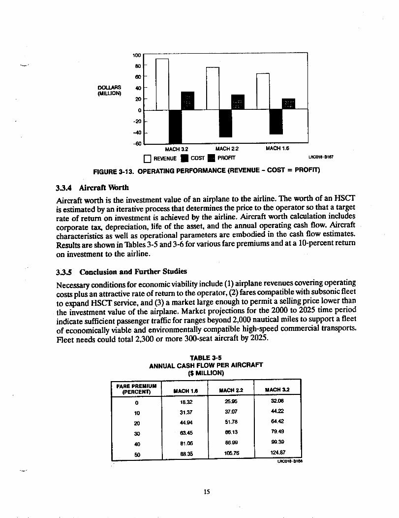
3.3.3 Operating Profit

Operating profit may be considered a measure of aircraft profitability. By deducting the oper-

ating cost from the revenues, operating profit can be calculated. Figure 3-13 shows the oper-

ating performance of the Mach 3.2, 2.2, and 1.6 configurations.

GENERALADMINISTRATION --_6.8

AIRCRAFT/ _. / / _._" /TRAFFIC _/'_ / 1/.l"1o /

SERVICING --"12.0%

CURRENTSUBSONIC

GENERALADMINISTRATION

6.5% __ _

,__/_ MAINTENANCEAIRCRAFT/TRAFFICSERVICING13.0% 9.1%

PASSENGER SERVICE9.0%

MACH 22LRCO18-B165

FIGURE 3-12. OPERATING COST BREAKDOWN - NO OWNERSHIP-RELATED COSTS

TABLE 3-4OPERATING COST DATA FOR MACH 1.6, 2.2, 3.2 AIRCRAFT

OPERATING COST PER SEAT-MILE ($)

OPERATING COST PER MILE ($)

OPERATING COST PER BLOCK HOUR ($)

OPERATING COST PER TRIP ($)

OPERATINGcoST PER AIRCRAFT PER YEAR ($)

MACH 1.6

0.135

15.51

14.414.00

64.686.00

44.9 MILUON

MACH 2.2

0.048

14.36

16.769.00

59.908.00

49.2 MILLION

MACH 3.2

0.047

14.18

21,711.00

59,162.00

59.2 MILLION

LRCO18-B186

14

DOLLARS(MILUON)

100

8O

6O

4O

20

0

-20

-40

--6OMACH 3.2 MACH 2.2 MACH 1.6

I-I . NUE II COSTII PRoFn" IJ_Ol_.B187

FIGURE 3-13. OPERATING PERFORMANCE (REVENUE - COST = PROFIT)

3.3A Aircraft Worth

Aircraft worth is the investment value of an airplane to the airline. The worth of an HSCT

is estimated by an iterative process that determines the price to the operator so that a targetrate of return on investment is achieved by the airline. Aircraft worth calculation includes

corporate tax, depreciation, life of the asset, and the annual operating cash flow. Aircraft

characteristics as well as operational parameters are embodied in the cash flow estimates.Results are shown in Tables 3-5 and 3-6 for various fare premiums and at a 10-percent return

on investment to the airline.

3.3.$ Conclusion and Further Studies

Necessary conditions for economic viability include (1) airplane revenues covering operating

costs plus an attractive rate of return to the operator, (2) fares compatible with subsonic fleet

to expand HSCT service, and (3) a market large enough to permit a selling price lower thanthe investment value of the airplane. Market projections for the 2000 to 2025 time period

indicate sufficient passenger traffic for ranges beyond 2,000 nautical miles to support a fleet

of economically viable and environmentally compatible high-speed commercial transports.

Fleet needs could total 2,300 or more 300-seat aircraft by 2025.

TABLE 3-5

ANNUAL CASH FLOW PER AIRCRAFT

FARE PREMIUM(PERCENT)

0

10

20

30

4O

50

($ MILLION)

MACH 1.6 MACH 2.2

18.32 25.95

31.37 37.07

44.94 51.78

63.45 66.13

81.06 86.99

88.35 105.76

MACH 3.2

32.08

44.22

64.42

79.49

99.39

124.87

LRCOIB-BI_.

15

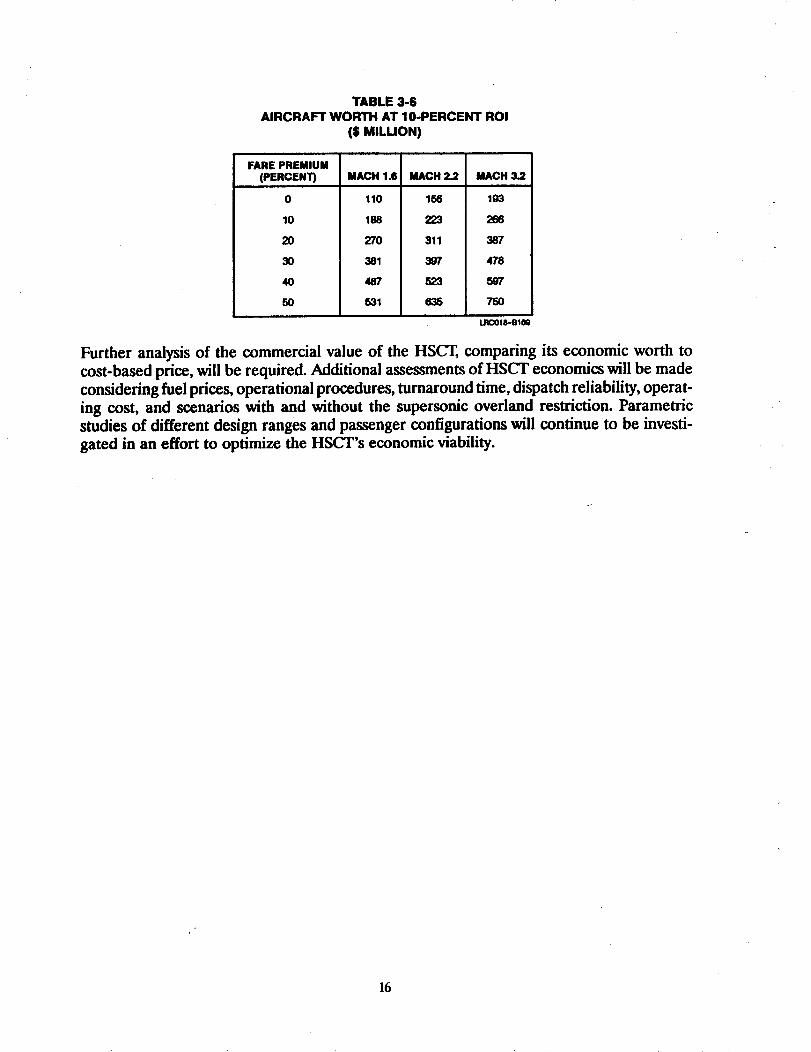
TABLE 3-6

AIRCRAFT WORTH AT 10-PERCENT ROI

($ MILLION)

FARE PREMIUM(PERCENT) MACH 1.6 MACH 2.2 MACH 3.2

0

10

20

30

4O

5O

110

188

270

381

487

531

166

223

311

397

523

635

193

266

387

478

597

75O

LRCO18-BI_

Further analysis of the commercial value of the HSCT, comparing its economic worth to

cost-based price, will be required. Additional assessments of HSCT economics will be madeconsidering fuel prices, operational procedures, turnaround time, dispatch reliability, operat-ing cost, and scenarios with and without the supersonic overland restriction. Parametricstudies of different design ranges and passenger configurations will continue to be investi-gated in an effort to optimize the HSCT's economic viability.

16

SECTION 4SUPERSONIC NETWORK EVALUATION

Future supersonic aircraft will bring major changes to long-range transportation. The newgeneration of aircraft will have to overcome many economic and environmental challengesbefore it can become a reality. The most constraining challenge is the global concern overthe effect of engine emissions on the ozone layer, which protects life on earth from ultravioletradiation. Community noise is another environmental challenge. The HSCT must meet atleast the current subsonic noise certification standards to be compatible with the future sub-

sonic fleet.

The sonic boom issue represents a major environmental and economic challenge as well.

Supersonic operation overland produces the most desirable economic results. However,unacceptable overland sonic boom characteristics may force HSCT to use subsonic speedsoverland.

Environmental concerns are likely to impose some restrictions on supersonic operation, thusintroducing major changes to existing route structures and supersonic network composition.Concern over the atmospheric effect may restrict HSCT's cruise altitude and its proximityto the denser ozone layers. It may also interfere with great circle routes because of environ-

mental impact on sensitive areas such as the North Pole. The current subsonic route structuremay have to be altered to avoid sensitive areas in the stratosphere or to minimize overlandflight tracks. It is important to examine the impact of these restrictions on the economic

viability of the overall supersonic operation.

To be profitable, a supersonic transport must offer the traveling public significant time savings

on long routes at acceptable fare premium levels. Under these assumptions, a potential mar-ket of about 2,000 aircraft will exist by the year 2025. This fleet size will enable engine and

airframe manufacturers to build the plane at a cost that provides them with an attractive

return on investment and to sell it at a price that allows the airlines to operate with a reason-

able profit.

Subsonic overland operation of a supersonic aircraft hinders its economic viability for the

following reasons:

Reduced time savings

Subsonic operation of a supersonic configuration imposes a penalty on its operating cost

(e.g., increased fuel burn)

Exclusion of some major city-pairs from the global supersonic network

Increased airline dependence on fare premiums, thus reducing the HSCT's potential

market share and profit

The effect of supersonic overland restriction on the aircraft's economic performance and

the development of supersonic network scenarios will be investigated and discussed in thissection.

17

4.1 AIRCRAFT ECONOMIC PERFORMANCE

4.1.1 Time Savings

Unrestricted supersonic operation produces optimum economic results. Time savings, the

HSCT's most attractive marketing feature, would be maximized. As the percentage of sub-

sonic overland increases, time savings decrease, thus eroding the unique competitive advan-

tage of the HSCT over subsonic aircraft. Figure 4-1 shows how time savings decline at differ-

ent levels of mixed operation. The highest time savings of supersonic versus subsonic flight

is achieved for routes that are entirely overwater, such as between Honolulu and Sydney,

where time savings exceed 5-1/2 hours. As the percentage of restricted operation increases,

time savings decline, as for example the Dallas Fort Worth-Frankfurt route, where time sav-

ings are cut to 3 hours.AVERAGE STAGE LENGTH -- 4.500 NAUTICAL MILES

BLOCK TIME(HOURS)

11

loi

9

6

5

4

SUBSONIC

I o

o

" ,,L'_ MACH 1.6

. -'-.-7 - .... "

-- -- MACH 3.23

uJ z

u) ,_ ci

O" I I I0 20 40 60

I

8O

OVERLAND OFF-DESIGN OPERATION (PERCENT)

100

FIGURE 4-1. TIME PERFORMANCE

OFF-DESIGNCRUISE SPEED

MACH 0.95

LRCO18-B105

4.1.2 Operating Cost and Profit

There is a significant reduction in aircraft economic performance when a mixed mode of

operation is gradually introduced. The impact of wholly supersonic versus mixed subsonic and

supersonic flight on the vehicle's operating economics is illustrated in Figure 4-2. The data

presented compare the operating revenue, cost, and profit for a vehicle with all Mach 2.2

operation versus vehicles with a mixed Mach number operation of Mach 2.2 overwater and

0.9 overland, or Mach 2.2 overwater and 1.6 overland. These comparisons are made with 10,

20, and 30 percent of the operation flown at the lower Mach number. At a 30:70 ratio of over-

land (Mach 1.6) to overwater (Mach 2.2) operation, there is an increase in operating cost of

$3 million annually per aircraft and $1.3 billion for the global fleet. This reduces the vehicle's

operating profit by the same amount. When the overland portion is flown at Mach 0.9, the

increase in operat!ng cost and the corresponding decrease in profit amounts to $5 million pervehicle annually and $2.2 billion for the global fleet.

18

O REVENUE

(REVENUE- COST ,, PROFIT)MACH 2.2, MACH 2.2/1.6, MACH 2.210.9 (PER AIRCRAFT)

D COST B PROFIT

DOLLARS(MILUON)

8O

70

60

50

4O

30

20

10

0

10

20

30

40

50

60

2125

54 52 50 49 50 51 52

MACH MACH MACH MACH MACH MACH MACH

2.2/0.9 (30%) 2.2/0.9 (20%) 2.2/0.9 (10%) 2.2 2.2/1.6 (10%) 2.2/1.6 (20%) 2.2/1.6 (30%)

LRCOtS-B106

FIGURE 4-2. OPERATING PERFORMANCE

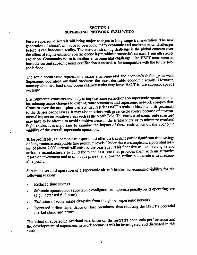
A sonic boom-minimized aircraft at Mach 1.6 will economically outperform a vehicle with

mixed operation of Mach 2.2 overwater and Mach 0.9 overland when the overland portion

exceeds 30 percent of the flight. Figure 4-3 shows the percentage of cost to revenue and profit

to revenue for Mach 2.2/1.6 and Math 2.2/0.9 configurations at different percentages of sub-

sonic operation. As the percentage of subsonic operation increases, the ratio of cost to reve-

nue rises, while the ratio of profit to revenue declines: These ratios are compared to those

of an all Math 1.6 configuration. The unrestricted Mach 1.6 profitability ratio becomes higher

than that of Mach 2.2/0.9 when the overland portion exceeds 28 percent, and higher than that

of Mach 2.2/1.6 when the overland portion exceeds 50 percent.

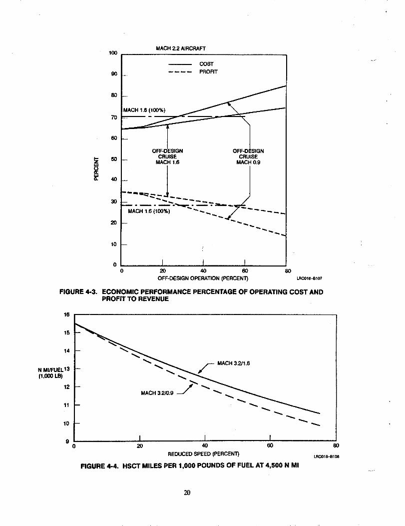
The increase in operating cost is mostly due to the higher fuel burn of the mixed Mach number

operation. Figure 4-4 illustrates the decline in HSCT miles per 1,000 pounds of fuel as the

percentage of mixed operation increases over an average stage length of 4,500 nautical miles.

For example, Mach 3.2 miles per 1,000 pounds of fuel burned declines by 13 percent when

20 percent of the operation is restricted to Mach 0.9 overland, and by 30 percent when the

restricted overland portion reaches 60 percent of the flight.

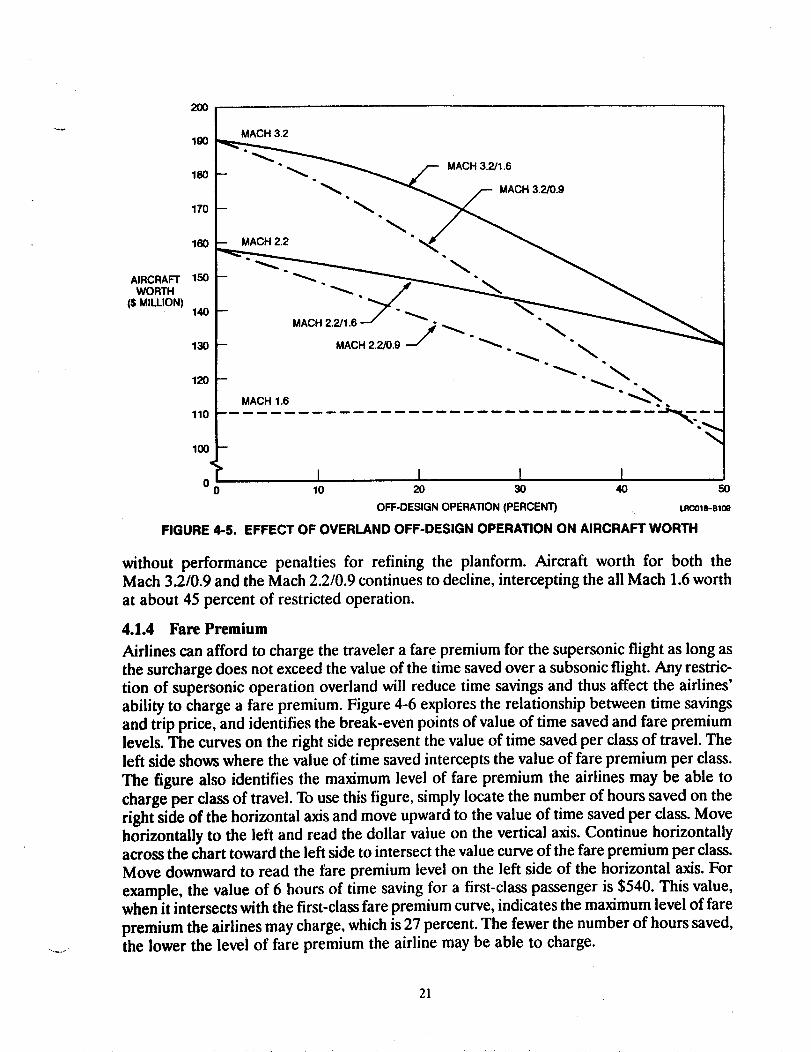
4.1.3 Aircraft Worth

Aircraft worth, which is the investment value of an airplane to the airline operator, is also

affected by restricted operation overland. An increase in the percentage of mixed Mach

number operation reduces aircraft worth. Figure 4-5 shows that aircraft worth reaches its

highest level at full supersonic operation. The data presented compare aircraft worth forvehicles with mixed Math number operation versus an all Math 1.6 sonic boom configuration

19

MACH 2.2 AIRCRAFT100

FIGURE 4-3.

90

8O

70

6O

5O

4O

3O

2O

10

COST

PROF_

OFF-D SIGNCRUISE CRUISE

MACH 1.6 MACH 0,9

/....... -.._- . _ . _ .._c_

MACH 1.6 (100%) " -- .. -. J -- " _ _ --- .. _

I I I0 20 40 60 80

OFF-DESIGN OPERATION (PERCENT) LRC018-8107

ECONOMIC PERFORMANCE PERCENTAGE OF OPERATING COST ANDPROFIT TO REVENUE

15

__ MACH 3.2/1.6

14

N MI/FUEL 13(1,000 LB)

12

11

10

90

FIGURE 4-4.

I I I2O 40 60

REDUCED SPEED (PERCENT)

HSCT MILES PER 1,000 POUNDS OF FUEL AT 4,500 N MI

8O

LRCO18-B108

2O

200

AIRCRAFTWORTH

($ MILLION)

lg0

180

170

180

150

140

130

120

110

100

00

FIGURE 4-5.

m

MACH 1.6

MACH 3.2

_ "_. _. __H 3.uo.9

MACH 2.2/1.6 _ _7: _ " _ "_

-- MACH 2.2]0.9 -- . _ --

ql

....

I I I I10 20 30 40 50

OFF-DESIGN OPERATION (PERCENT) LRCOle-B10e

EFFECT OF OVERLAND OFF-DESIGN OPERATION ON AIRCRAFT WORTH

without performance penalties for refining the planform. Aircraft worth for both theMach 3.2/0.9 and the Math 2.2/0.9 continues to decline, intercepting the all Mach 1.6 worth

at about 45 percent of restricted operation.

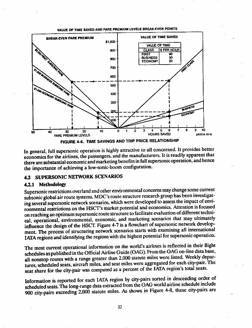
4.1.4 Fare Premium

Airlines can afford to charge the traveler a fare premium for the supersonic flight as long asthe surcharge does not exceed the value of the time saved over a subsonic flight. Any restric-tion of supersonic operation overland will reduce time savings and thus affect the airlines'ability to charge a fare premium. Figure 4-6 explores the relationship between time savingsand trip price, and identifies the break-even points of value of time saved and fare premium

levels. The curves on the right side represent the value of time saved per class of travel. Theleft side shows where the value of time saved intercepts the value of fare premium per class.

The figure also identifies the maximum level of fare premium the airlines may be able to

charge per class of travel. To use this figure, simply locate the number of hours saved on the

right side of the horizontal axis and move upward to the value of time saved per class. Movehorizontally to the left and read the dollar value on the vertical axis. Continue horizontallyacross the chart toward the left side to intersect the value curve of the fare premium per class.

Move downward to read the fare premium level on the left side of the horizontal axis. For

example, the value of 6 hours of time saving for a first-class passenger is $540. This value,when it intersects with the first-class fare premium curve, indicates the maximum level of fare

premium the airlines may charge, which is 27 percent. The fewer the number of hours saved,the lower the level of fare premium the airline may be able to charge.

21

VALUE OF TIME SAVED AND FARE PREMIUM LEVELS BREAK-EVEN POINTS

BREAK-EVEN FARE PREMIUM$1.000'

VALUE OF TIME SAVED

VALUE OF TIME

I50 40 30 20 10 0 1 2 3 4 5 6 7 8 9 10

FARE PREMIUM LEVELS HOURS SAVED LRCOle-B.0

FIGURE 4-6. TIME SAVINGS AND TRIP PRICE RELATIONSHIP

In general, full supersonic operation is highly attractive to all concerned. It provides bettereconomies for the airlines, the passengers, and the manufacturers. It is readily apparent that

there are substantial economic and marketing benefits in full supersonic operation, and hence

the importance of achieving a low-sonic-boom configuration.

4.2 SUPERSONIC NETWORK SCENARIOS

4.2.1 Methodology

Supersonic restrictions overland and other environmental concerns may change some current

subsonic global air route systems. MDC's route structure research group has been investigat-

ing several supersonic network scenarios, which were developed to assess the impact of envi-ronmental restrictions on the HSCT's market potential and economies. Attention is focused

on reaching an optimum supersonic route structure to facilitate evaluation of different techni-

cal, operational, environmental, economic, and marketing scenarios that may ultimately

influence the design of the HSCT. Figure 4-7 is a flowchart of supersonic network develop-

ment. The process of structuring network scenarios starts with examining all international

IATA regions and identifying the regions with the highest potential for supersonic operation.

The most current operational information on the world's airlines is reflected in their flight

schedules as published in the Official Airline Guide (OAG). From the OAG on-line data base,

all nonstop routes with a range greater than 2,000 statute miles were listed. Weekly depar-tures, scheduled seats, aircraft miles, and seat miles were aggregated for each city-pair. The

seat share for the city-pair was computed as a percent of the IATA region's total seats.

Information is reported for each IATA region by city-pairs sorted in descending order of

scheduled seats. The long-range data extracted from the OAG world airline schedule include

900 city-pairs exceeding 2,000 statute miles. As shown in Figure 4-8, these city-pairs are

22

Ail CITY-PAI_ 1.000 CITY-PAIRS>2,000 ST MI _ 19 IATA REGIONS

OAG JULY 1990/

RANK CITY-PAIRS_ I

BY CAPACITYFOR NETWORK _ ISELECTION / L

1FOR OVERLAND /'"]MIN,MIZAnON/ I

ISUPERSONIC OVERWATER I

ONLY - CITY-PAIRS WITH< 6-PERCENT OVERLAND

UNRESTRICTEDSUPERSONIC

NETWORKS

r 1

• r% C -PA,RS.";'I 25o CITY-PAIRS | I" /150CITY-PAIRS I I-.=

UST OF 250 CITY-PAIRSRANKED BY CAPACITY AND

MINIMUM OVERLAND PORTION

EXTRACT APPROPRIATERESTRICTED NETWORK

SCENARIOS

I ITHAT AVERAGE IO-PERCENT WITH DEDICATED

OVERLAND = CORRIDORS

I AVERAGE 20-PERCENT I IL -- --. OVERLAND j =......

FIGURE 4-7.

1.000

SUPERSONIC NETWORK SCENARIOS FOR UNRESTRICTEDAND RESTRICTED OPERATION

TRAFFIC ON ROUTES LONGER THAN 2,000 ST MI

900

8OO

700

I OAG DATA FOR JUNE 1990 I

6OO

NUMBER OFAIRPORT-PAIRS 500

4O0

3O0

II

J

LRC018-B111

!

IATA REGIONNO. J

18

1412

1110

9

20O

100

060 55 60 66 70 75 80 85 90

TOTAL WEEKLY SEATS OFFERED BY REGION (PERCENT)

FIGURE 4-8. TRAFFIC ANALYSIS BY IATA REGIONS

95

3

21

100

LRCO18-B112

23

distributed among 14 IATA regions. Not all of these city-pairs are necessarily candidates for

HSCT service. The most logical candidates are the high-density traffic routes, defined by

scheduled seat capacity.

Using the long-range data set, sorted in descending order of scheduled seats, many subsets

of top city-pairs can be selected as unrestricted supersonic network scenarios. These super-

sonic network scenarios can only be used if a low-boom configuration is successfully devel-

oped. To visualize the global network formed by the top 250 city-pairs, their great circle routes

were plotted on a world map in Figure 4-9.

4.2.2 Route Diversion Analysis

Until a satisfactory solution to the sonic boom problem is obtained, supersonic flight overland

will be restricted. Modifications to great circle routes are required to find an alternative flight

path that eliminates or minimizes overland flight to unpopulated land masses. Using the long-

range data set, a subset of the top 250 city-pairs was selected to conduct route diversion analy-

ses. The basic traffic data for the 250 city-pairs are presented in Appendix A. The traffic data

are also sorted by departures, aircraft miles, annual seat miles, and aircraft hours. This rank-

ing highlights the fact that membership in the top set is controlled by the choice of rankingcriteria.

The 250 candidate city-pairs route were each analyzed for possible diversion to eliminate or

reduce overland tracks. The process involved generating a strip chart for each candidate

route. A strip chart is an oblique map projection showing an area 15 to 20 degrees on either

side of the great circle track between origin and destination. By selecting the great circle route

to be the equator of the projection, the highest possible scale accuracy is obtained for the

chart. From such charts, diverted routes can be designed, and overland segments, if any, can

be measured directly. Figure 4-10 shows the strip chart for the London-New York route. Data

presented in Figure 4-10 show that the overland track has been reduced more than 20 percent

through diversion, while the increase in great circle distance is limited to only 3 percent. The

generated strip charts of a few key routes are presented in Appendix B.

The results of the route diversion analysis are summarized in Appendix C. The table compares

the overland portions of the diverted route and its original great circle route. Some of the

routes are all overwater with no diversion required. Others become all overwater through

diversion. Still others exhibit various degrees of overland reduction through diversion. How-

ever, some are all overland, where no feasible diversion is possible. The all-overland routes

are strong candidates for removal from possible HSCT service.

In evaluating flight performance, the ground track profile becomes important. If the overland

segments of the route occur at the beginning and end of the flight, performance is least

affected. However, if the overland segments happen to fall anywhere along the track after

cruise speed has been reached, performance penalties can be severe. The aircraft must fly

lower and slower over the land segment and then climb back up to higher cruise altitude. The

amount of fuel burned by this maneuver depends on how heavy the aircraft is at the start of

the maneuver. The ground track profiles on a normalized linear scale are summarized in

Appendix C. Each track profile is flagged according to the type it exhibits. Type 1 profile is

all overwater or has overland portions at either end of the track. Type 2 is a profile with over-

24

: l

BGI

GIG

NBO\\

NB

-_'RUN \ \\

l\

AVERAGE STAGE LENGTH 3,666 ST MI

1. NORTH AMERICA - SOUTH AMERICA (5)GIG-MIA NO. 20

2. NORTH AMERICA - CENTRAL AMERICA (6)JFK-MEX NO. 61

3. NORTH TRANSATLANTIC (69)JFK-LHR NO. 2

4. MID TRANSATLANTIC (10)MAD-MIA NO. 132

S. SOUTH TRANSATLANTIC (3)GIG-MAD NO. 120

PERCENT OF LONG-RANGE TRAFFIC -- 70 PERCENT

7. EUROPE - SOUTH AFRICA (3)JNB-LHR NO. 101

8. EUROPE - MIDDLE EAST (12)DXB-LON NO. 78

9. EUROPE - FAR EAST (26)NRT-SVO NO. 24

10. AMERICAS - MID PACIFIC (23)HNL-NRT NO. 10

11. AMERICAS - SOUTH PACIRC (5)AKL-HNL NO. 50

12. WITHIN NORTH AMERICA (55)HNLoLAX NO. 1

16. WITHIN AFRICA (1)JIB-RUN NO. 245

18. WITHIN FAR EAST (25)NRT-SIN NO. 12

19. MISCELLANEOUS (8)BKK-DXB NO. 84

FIGURE 4-9, TOP 250 POTENTIAL SUPERSONIC ROUTES (NO RESTRICTIONS) u_o_2-,

BEFOREDIVERSION:GREATCIRCLEDISTANCE2.990NMI

_.

MILES OVERLAND PERCENT OVERLAND831 N MI 27.8%

° 6

GREAT CIRCLEDIVERTED

AFTER DIVERSION: MILES OVERLAND PERCENT OVERLANDDIVERTED DISTANCE 221 N MI 7.2%

3.076 N MI LRCOlS-a113

FIGURE4-10. CITY-PAIREVALUATION- JFK (NEWYORK)-LHR(LONDON)

land segments anywhere in the middle of the track. Type 3 consists of tracksexhibiting more

than 50 percent of overland segments, which are candidates for elimination. Type 4 identifiestracks that are 100-percent overland. An example of route diversion and optimization isdepicted in Figure 4-11 for the New York-Tokyo route. By rerouting the flight via Seattle,

distance increased by 693 miles, and the percentage overland declined from 88 to 35 percent,as illustrated in Figure 4-11A. By diverting the route through the Arctic Ocean, Bering Strait,and North Pacific, the percentage of overland flight was further reduced to 20 percent at acost of 227 extra nautical miles, as shown in Figure 4-11B. The ground track profile is dis-

played on a normalized scale in Table 4-1.

The 250-network scenario represents 64 percent of the annual seat-miles for long-rangeroutes over 2,000 statute miles. The average impact of route diversion compared to the great

circle route is a 4-percent increase in network distance and a 41-percent reduction in overlanddistance. To visualize the global network formed by the top 250 city-pairs, their great circle

routes were plotted on a world map in Figure 4-12. A 150 city-pair network is also considered

as a candidate supersonic scenario. The 150-network scenario is similar to the 250 city-pairscenario without the bottom 100 city-pairs. The 150-network scenario represented 52 percent

of the annual seat-miles for all long-range routes over 2,000 statute miles. Although the i50

city-pair network is structurally only 60 percent of the 250 city-pair network, 80 percent of

the traffic is still present. The average impact of route diversion compared to the great circle

routes is a 5-percent increase in network distance and a 41-percent reduction in overland dis-

tance. The great circle routes for the 150 city-pair network are shown in Figure 4-13. The most

apparent feature, when the map is compared to the 250-network map, is that the global pat-tern does not change, but gets denser.

26

A. VIA SEATTLE

I

I

EXTRA MILES 693OVERLAND MILES 2,288PERCENT OVERLAND 35%BLOCK TIME 7.1 HR

B. VIA BERING STRAIT

.... GREAT CIRCLE _ _ __

•-._N o-

DIVERTED DISTANCE 6,072 N M, _'__._

FOR THIS DIVERTED ROUTE: _ ( f_EXTRA MILES 227OVERLAND MILES 1,190PERCENT OVERLAND 19.61%BLOCK TIME 5.5 HR LRCOIS-B_7

FIGURE 4-11. DIVERTED ROUTING - NEW YORK-TOKYO

4.2.3 Overwater Network Scenario

The basic HSCT 250-network scenario was based on the high-density traffic as reported by

the OAG. The ground track display shows a mix of desirable and undesirable flight profiles,and some routes that exhibit a high percentage of overland portions. The 250 city-pairs listsorted in descending order of scheduled seats in Appendix A was resorted in ascending order

of percentage of the overland segment, as shown in Appendix C. All routes exhibiting morethan half the distance overland were eliminated. A list of 207 city-pairs, with an overland por-

tion that does not exceed half the distance in each case, was used to extract a variety of super-

sonic notwork scenarios. For example, to extract an ali-overwater network, only routes with

a 6-percent overland segment, 3 percent for climb and 3 percent for descent, would be

27

TABLE 4-1,

EXAMPLE OF GROUND TRACK PROFILE DISPLAY FOR NEW YORK-TOKYO

GCAIRPORT RANGE DIVERTED OVERLAND

PAIR (N MI) RANGE DIST (%) FLAG

UM-MIA 2,277 2,647 183 6.9 2CPH-SEA 4,214 5,074 624 12.3 2LHR-NRT 5.147 5.880 759 129 2EZE-MIA 3.831 4,137 691 16.7 2FRA-NRT 5,063 5.211 917 17.6 2JFK-NRT 5,845 6,072 1,1g0 19.6 2COG-NRT 6,237 5,607 1,110 19.8 2LAX-LHR 4,727 5,138 1.978 38.5 2LAX-LGW 4,747 5,138 1.978 38.5 2BKK-DXB 2,635 2,635 1.415 53.7 2MEL-SIN 3,260 3,260 1.757 53.9 3BKK-KHI 1,998 1,998 1,451 72.6 3LHR-.SIN 5,872 5.872 4,886 83.2 3NRT-SVO 4.048 4,048 3,663 g0.5 3BKK-FCO 4,775 4,775 4,775 100.0 4

GROUND TRACK LENGTH (%)1

0 1 2 3 4 5 6 7 8 9 0

o., o ,° o ,o,,o, o o o .o,, ,o, |,,,, ,, ,,,i,,, , , , ,,,,,,,., ,,i ,,, i ,

I IIIII IIIII IIIIIIIIIIIII II IIIIIIIIIIIIII IIIII IIIIIIIIIIIIIIIIIIIIIIIIIII III IIIIIIIIIIIIIIIIIIIIII III III

IIIIIIIIII

IIIIIIII IIIIIIIIIIII IIIIIIIIIIIIIIIIII IIIIIIIIIIIII IIIIIIII IIIIIIIIIIIIIIIIIIIIIIIIIIIIIIIIIIIIIIIIIIIIIIIIIIIIIIIIIIIIIIIIIII I IIIIIIII IIIIIIIIIlilllllllllllllllllllllllllllllllllIIIIIIIIIIIIIIIIIIIIIIIIIIIIIIIIIIIIIIIIIIIIIIIIIIIt11111111111111111111111111111111111@1111111111_111t

LRCOtB-BO

selected. Under these assumptions, only 100 city-pairs would qualify for the overwater net-

work scenario. Figure 4-14 shows the great circle routes of the 100 city-pair overwaternetwork. The 100 overwater network represents 28 percent of total long-range annual seat-

miles. The average impact of route diversion compared to the great circle route is a 6-percentincrease in network distance and a 92-percent reduction in overland distance.

To structure a network with an overland portion averaging 10 percent of the total network,

the top 200 city-pairs are selected from the same list. The 200 network carries 50 percent oflong-range annual seat-miles. It covers 13 IATA regions and has an average stage length of

3,998 statute miles. An increase of 5.7 percent in distance results in a 69-percent reduction

in overland segments. Figure 4-15 illustrates the great circle route structure of the 200 city-pairs on the world map.

43 CONCLUSION

Only a few candidate global airline network scenarios for HSCT have been assembled. Theyare patterned after the high-density long-range markets from the OAG on-line data base.

Creative rerouting was conducted to minimize overland segments and to lessen the impact

of the environmental restrictions that may be imposed on future supersonic operation.

The data on these network scenarios represent an assembly of global routes from which

HSCT global traffic networks can be constructed. The network scenarios provide examples

on how supersonic service may bring some changes to the current global route structure.Some of these supersonic network scenarios show good potential of capturing more than half

the market share of the long-range traffic.

4.4 RECOMMENDATIONS FOR FURTHER STUDY

Further analysis is still required to accurately assess the effect of these supersonic networkscenarios on aircraft economic performance, productivity, and fleet projections. Supersonicnetwork research and development will continue to search for more ways to respond to theenvironmental concerns, operational policies, marketing strategies, and specific network

requirements of customer airlines.

28

J

//

/

SLC

GIG

\

\ t\ /\ /"

\ /\ /"

RANGES • 2,000 ST MILES FROM OAG FOR JULY 1990

LRC012-92

FIGURE 4-12. HSCT TOP SEAT RANK 250 AIRPORT-PAIRS

I/

/

/

# SLC

GUA

i;t

//

//

GIG

"ZE

MINUS IATA 12 AND RANGES • 2,000 ST MILES FROM OAG FOR JULY 1990 t

LRC012-91

FIGURE 4-13. HSCT TOP SEAT RANK 150 AIRPORT-PAIRS

i

PDX

/>

GIG

DEI_


1. NORTH AMERICA - SOUTH AMERICA (4)GIG-JFK NO. 16

2. NORTH AMERICA - CENTRAL AMERICA (3)BGI-JFK NO. 19

3. NORTH TRANSATLANTIC (26)JFK-CDG NO. 80

4. MID TRANSATLANTIC (5)

MAD-MIA NO. 99

PERCENT OF LONG-RANGE TRAFFIC - 28 PERCENT

5. SOUTH TRANSATLANTIC (5) 18.GIG-MAD NO. 87

19.10. AMERICAS - MID PACIFIC (19)

HNL-NRT NO, 2

11. AMERICAS - SOUTH PACIFIC (6)

AKL-HNL NO. 10

12. WITHIN NORTH AMERICA (8)HNL-LAX NO. 1

WITHIN FAREAST (20)NRT-SIN NO. 6

MISCELLANEOUS (4)DXB-KUL NO. 68

LRCO12.-g5

FIGURE 4-14. 100 CITY-PAIRS FOR OVERWATER ONLY - SUPERSONIC NETWORK

t_t_

/

////"

/ /

= IP'HNLI/" /

i i I/I /

t "l" / 1/ /

/ I� / /

,I i fJPPTI

II

/I

II

UM

/

I

II

/

I

I

I

GIG

I/I

IIi

\\\

RUN

OVERLAND PORTION AVERAGES 10 PERCENT OF TOTAL NETWORK

i vI

I1


1. NORTH AMERICA - SOUTH AMERICA (7)GIG-MIA NO. 69

2. NORTH AMERICA - CENTRAL AMERICA (6)JFK-MEX NO. 89

3. NORTH TRANSATLANTIC (83)JFK-LHR NO. 112

4. MID TRANSATLANTIC (14)MAD-MIA NO. 99

5. SOUTH TRANSATLANTIC (5)GIG-MAD NO. 87

PERCENT OF LONG-RANGE TRAFFIC - 50 PERCENT

8. EUROPE - MIDDLE EAST (5) 16.I.HR-TLVNO. 180

9. EUROPE - FAR EAST (5) 18.U-IR-NFIT NO. 142

10. AMERICAS - MID PACIFIC (28) 19.HNLoNRT NO. 2

11. AMERICAS - SOUTH PACIFIC (6)AKL-HNL NO. 26

12. WITHIN NORTH AMERICA (14)HNL-LAX

WITHIN AFRICA (1)JIB-RUN NO. 177

WITHIN FAR EAST (22)NRT-SIN NO. 6

MISCELLANEOUS (4)DXB-KUL NO. 68

LRC012-94

FIGURE 4-15. SUPERSONIC NETWORK SCENARIO FOR 200 CITY-PAIRS

SECTION 5

ATMOSPHERIC EMISSIONS IMPACT STATUS

Atmospheric emissions impact studies focused on generating inputs for two-dimensional

global atmospheric chemistry models. Airframe concepts at Mach 1.6, Mach 2.2, and

Mach 3.2 were used in conjunction with several low-NOx candidate engine concepts from

both Pratt & Whitney and General Electric. The procedure used to generate the atmospheric

model inputs was upgraded and automated under independent research funds. A brief

description of the procedure is included in this report and a complete description of the new

methodology is provided in NASA CR 181882.

The impact of atmospheric emissions for airframe/engine concepts on global ozone concen-

trations was estimated through correlation with Lawrence Livermore National Laboratories

(LLNL) two-dimensional (2-D) atmospheric model runs. Alarge matrix of emission scenarios

was provided to LLNL by Douglas under an independent research effort, and estimates of

global ozone impact were generated with the LLNL two-dimensional global atmospheric

model. The emissions scenarios developed for the 1990 emission studies were

cross-referenced with the independent research results to arrive at an estimated global ozone

column change. These estimates are included in this report.

The potential impact of regulations restricting cruise altitude was investigated in terms of eco-

nomic penalties and ozone benefits. Baseline aircraft at Math 1.6, 2.2, and 3.2 were flown

with several different cruise altitude ceiling limits. Fuel burn and emission constituent data

were generated for these restricted flight paths and compared to baseline cases. The ozone

impact of these restrictions was then estimated by cross-referencing the results with the LLNL

2-D model runs described above. Economic impact in terms of operating cost and aircraft

worth were quantified. These studies provide insight into the feasibility and practicality of

protecting atmospheric ozone through cruise altitude restrictions.

5.1 BRIEF METHODOLOGY REVIEW

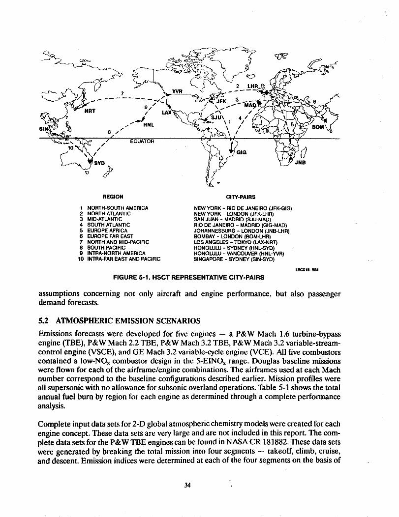
The operational network of an HSCT is broken down into 10 IATA regions worldwide. For

each of these regions, a city-pair is chosen that best describes the average latitude distribu-

tion. The 10 regions, along with their corresponding city-pairs, are shown in Figure 5-1. A

mission is flown for each city-pair with the airframe/engine combination in question to deter-

mine the fuel burn in each region as a function of altitude and latitude. The 10 regions are

then compiled into one data set representing the total annual worldwide fuel burn in each

latitude and altitude band as specified by the 2-D atmospheric models.

Final input to the global atmospheric models is broken down into seven distinct engine emis-sion constituents. These are NO, NO2, SO2, CO, H20, CO2, and THC (trace hydrocarbons).

In addition, summary data for all oxides of nitrogen are provided (NO + NO2) as NOx. The

total constituent emissions are determined by multiplying the total fuel burn by the emission

index for each constituent.

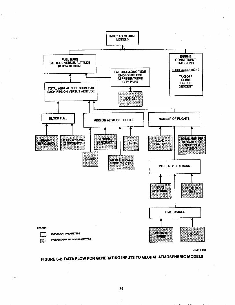
The worldwide fuel burns are a function of many parameters, including economic forecasts

for the time period in question. An overall data flowchart is presented in Figure 5-2. This

chart shows the dependency of the emissions data on a wide array of estimates and

33

, _-,_._ .. - __,,' "__)_ --'%

' "q_" _'_ _"_/ D<_10 _v"/_-"_" SY/" / '¢ EOUATOR _G IG _jN_ B

REGION CITY-PAIRS

1 NORTH-SOUTH AMERICA

2 NORTH ATLANTIC3 MID-ATLANTIC

4 SOUTH ATLANTIC

5 EUROPE AFRICA

6 EUROPE FAR EAST7 NORTH AND MID-PACIFIC

8 SOUTH PACIFIC9 INTRA-NORTH AMERICA

10 INTRA-FAR EAST AND PACIFIC

NEW YORK - RIO DE JANEIRO (JFK-GIG)NEW YORK - LONDON (JFK-LHR)

SAN JUAN - MADRID (SJU-MAD)

RIO DE JANEIRO - MADRID (GIG-MAD)

JOHANNESBURG - LONDON (JNB-LHR)BOMBAY- LONDON (BOM-LHR)

LOS ANGELES - TOKYO (LAX-NRT)

HONOLULU - SYDNEY (HNL-SYD)HONOLULU - VANCOUVER (HNL-YVR)

SINGAPORE - SYDNEY (SIN_SYD)

FIGURE 5-1. HSCT REPRESENTATIVE CITY-PAIRSLRCOt8-B54

assumptions concerning not only aircraft and engine performance, but also passengerdemand forecasts.

5.2 ATMOSPHERIC EMISSION SCENARIOS

Emissions forecasts were developed for five engines -- a P&W Mach 1.6 turbine-bypass

engine (TBE), P&W Mach 2.2 TBE, P&W Mach 3.2 TBE, P&W Mach 3.2 variable-stream-

control engine (VSCE), and GE Mach 3.2 variable-cycle engine (VCE). All five combustors

contained a low-NOx combustor design in the 5-EINOx range. Douglas baseline missions

were flown for each of the airframe/engine combinations. The airframes used at each Mach

number correspond to the baseline configurations described earlier. Mission profiles were

all supersonic with no allowance for subsonic overland operations. Table 5-1 shows the total

annual fuel burn by region for each engine as determined through a complete performance

analysis.

Complete input data sets for 2-D global atmospheric chemistry models were created for each

engine concept. These data sets are very large and are not included in this report. The com-

plete data sets for the P&W TBE engines can be found in NASA CR 181882. These data sets

were generated by breaking the total mission into four segments -- takeoff, climb, cruise,

and descent. Emission indices were determined at each of the four segments on the basis of

34

I

FUEL BURN l

LATITUDE VERSUS ALTITUDE10 IATA REGIONS

1 t/

TOTAL ANNUAL FUEL BURN FOR IEACH REGION VERSUS ALTITUDE /

J1 1T

I BLOCK FUEL

DEPENDENT PARAMETERS

INDEPENDENT (BASIC) PARAMETERS

I INPUT TO GLOBALMODELS

LATITUDE/LONGITUDEENDPOINTS FORREPRESENTATIVE

CITY-PAIRS

LEGEND:

F-1D

]

li!!iiillii!iiiiiiil

MISSION ALTITUDE PROFILE

IENGINE

CONSTITUENTEMISSIONS

TAKEOFFCLIMB

CRUISEDESCENT

I NUMBER OF FUGHTS

I

IIii__iiiillii!iiiliiii_!iili!il

PASSENGER DEMAND

T

I TIME SAVINGS I

!...._......L _i_ii!iii!ill

FIGURE 5-2. DATA FLOW FOR GENERATING INPUTS TO GLOBAL ATMOSPHERIC MODELS

35

data supplied by the engine manufacturers. This is believed to improve the fidelity of the emis-

sions estimates compared to methods that consider only the cruise segment. NOx, emission

indices for each

Table 5-2.

engine concept at the various operating conditions

REGION

NORTH-SOUTH AMERICA

NORTH ATLANTIC

MID-ATLANTIC

SOUTH ATLANTIC

EUROPE-AFRICA

EUROPE-FAR EAST

NORTH AND MID-PACIFIC

SOUTH PACIFIC

INTRA-NORTH AMERICA

INTRA-FAR EAST AND PACIFIC

TABLE 5-1

TOTAL ANNUAL FUEL BURN BY REGION

FUEL BURN (106 LB)

P&WMACH 1.6

TBE

1.729

20.029

1,445

2.262

4,339

6,805

23.992

2,612

159

10,390

P&WMACH 2.2

TBE

1.735

20.168

1.453

2.255

4,391

6.814

23,934

2,618

163

10,527

P&WMACH 3.2

TBE

1,864

21,774

1.565

2.393

4,791

7.283

25.411

2.806

182

11,487

P&WMACH 3.2

VSCE

2,371

27,656

1,985

3,039

6.110

9,224

32,261

3,563

231

14.594

are presented in

GEMACH 3.2

VCE

2,133

24.889

1,768

2,730

5,493

8,296

28.968

3.202

209

13,133

TABLE 5-2

NOx EMISSION INDICES FOR VARIOUS ENGINE CONCEPTS

El = LBI1,000 LB FUEL BURNED

ENGINE TAKEOFF CLIMB CRUISE DESCENTEl El El El

P&W MACH 1.6 TBE

P&W MACH 2.2 TBE

P&W MACH 3.2 TBE

P&W MACH 3.2 VSCE

GE MACH 3.2 VCE

5.5

3.5

3.5

2.3

3.6

6.7

6.1

7.9

4.5

7.8

5.3

4.5

5.1

4.4

6.3

3.7

2.7

1.5

4.5

10.1

LRC018-B56

5.3 OZONE IMPACT TRADE STUDIES

The baseline emissions scenarios developed for this task were used in conducting trade

studies to investigate the effects of parameters such as fleet size, fare premium, Math number,

year of service, and engine type on the global ozone concentration as predicted by the LLNL

2-D model (through correlation with IRAD data).

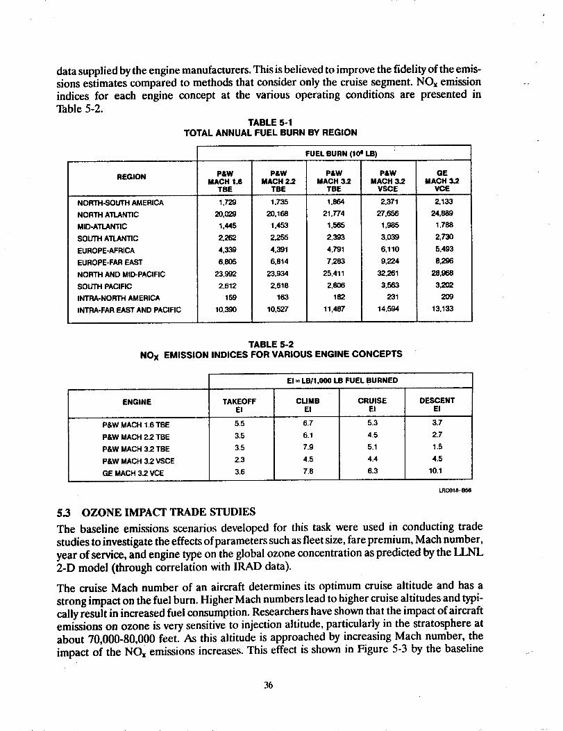
The cruise Mach number of an aircraft determines its optimum cruise altitude and has a

strong impact on the fuel burn. Higher Mach numbers lead to higher cruise altitudes and typi-

cally result in increased fuel consumption. Researchers have shown that the impact of aircraft

emissions on ozone is very sensitive to injection altitude, particularly in the stratosphere at

about 70,000-80,000 feet. As this altitude is approached by increasing Mach number, the

impact of the NOx emissions increases. This effect is shown in Figure 5-3 by the baseline

36

OZONEDEPLETION

(%)

f

MACH 3.2

MACH 2.2

MACH 1.6

02OOO 2010 2O2O 2O30

YEAR LRO01_7

FIGURE 5'3. OZONE DEPLETION BY YEAR - P&W TBE ENGINE

emissions scenarios. From this plot, it is readily seen that column ozone depletion is a strongfunction of Mach number. The figure also shows that ozone concentration is furtherdecreased as the fleet size is increased over a period of production years. In the 20 years from2005 to 2025, the ozone impact of HSCT emissions based on passenger demand may be

expected to increase by a factor of four.

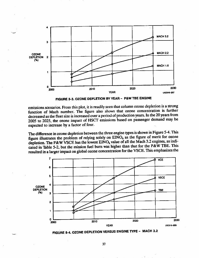
The difference in ozone depletion between the three engine types is shown in Figure 5-4. This

figure illustrates the problem of relying solely on EINOx as the figure of merit for ozonedepletion. The P&W VSCE has the lowest EINOx value of all the Mach 3.2 engines, as indi-cated in Table 5-2, but the mission fuel burn was higher than that for the P&W TBE. Thisresulted in a larger impact on global ozone concentration for the VSCE. This emphasizes the

OZONEDEPLETION

(%)

7

6

5

4

3

2

1

02000

f VCE

j l VSCE

TBE

2010 202O

YEAR

FIGURE 5-4. OZONE DEPLETION VERSUS ENGINE TYPE - MACH 3.2

203O

LRCOlS-B58

37

need for the engine manufacturers to maintain high cruise efficiency while improving EINOxcombustor standards.

A direct comparison of fleet size, number of flights, and ozone depletion is shown in Fig-

ure 5-5. The ozone depletion for a given fleet size is found by cross-referencing the fleet size

with the number of flights for the appropriate Mach number. The number of flights can then

be translated vertically to the top plot to determine the column ozone depletion. For a given

annual passenger demand, and hence number of flights, the ozone impact is greater for aMath 3.2 fleet than for a Mach 1.6 fleet, even though the Mach 3.2 fleet is smaller.

Logically, it would be assumed that a larger fleet size would lead to a greater ozone impact.

This is not always the ease, however, because the important parameter is actually the number

of flights. One aircraft making 1000 annual flights will have a greater ozone impact than 500

aircraft making one annual flight. This effect is important when comparisons are made for

different Mach numbers. Faster airplanes can make more flights per day, thereby allowing

for smaller fleet sizes to achieve equal productivity. Therefore, the Mach 3.2 fleet is smaller

0

3.000

OZONEDEPLETION

(%)

FLEET 2,000SIZE

1,000

MACH 3.2

J

o---'"

MACH 2.2

MACH 1.6

MACH 1.6J _ MACH 2.2

0.5 1.0 1.5 2.0

NUMBER OF FLIGHTS (MILLION) LRCOtS-B,_

FIGURE 5-5. OZONE DEPLETION AND FLEET SIZE VERSUS NUMBER OF FLIGHTS

FOR P&W TBE

38

than the Mach 2.2 or Mach 1.6 fleet for an equivalent number of annual flights and equal

productivity.

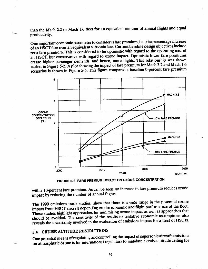
One important economic parameter to consider is fare premium, i.e., the percentage increaseof an HSCT fare over an equivalent subsonic fare. Current baseline design objectives include

zero fare premium. This is considered to be optimistic with regard to the operating cost of

an HSCT, but conservative with regard to ozone impact. Optimistic lower fare premiums

create higher passenger demands, and hence, more flights. This relationship was shown

earlier in Figure 5-2. A plot showing the impact of fare premium for Mach 3.2 and Mach 1.6scenarios is shown in Figure 5-6. This figure compares a baseline 0-percent fare premium

OZONECONCENTRATION

DEPLETION

(%) 2

_000

j MACH 3.2

PREMIUM

MACH 1.6_r

_-10% FARE PREMIUM

2010 2020 2030

YEAR LRCOIS-BeO

FIGURE 5-6. FARE PREMIUM IMPACT ON OZONE CONCENTRATION

with a 10-percent fare premium. As can be seen, an increase in fare premium reduces ozone

impact by reducing the number of annual flights.

The 1990 emissions trade studies show that there is a wide range in the potential ozone

impact from HSCT aircraft depending on the economic and flight performance of the fleet.

These studies highlight approaches for minimizing ozone impact as well as approaches that

should be avoided. The sensitivity of the results to tentative economic assumptions also

reveals the uncertainty involved in the evaluation of emissions impact for a fleet of HSCTs.

5.4 CRUISE ALTITUDE RESTRICTIONS

One potential means of regulating and controlling the impact of supersonic aircraft emissions

on atmospheric ozone is for international regulators to mandate a cruise altitude ceiling for

39

supersonicflight, ensuringthat NOx is not emitted in themore sensitivealtitude bands.Theeconomicand performance impactsof sucha regulation are strongly influenced by Mathnumber, optimum cruise altitude of the aircraft, and the cruise restriction altitude. Forinstance,a 60,000-footceiling restriction isnot likely to haveanyimpacton a Math 1.6con-

figuration, but would significantly erode the performance of a Mach 3.2 configuration and,

to a lesser extent, that of the Mach 2.2 configuration.

A series of cruise altitude restrictions were applied to the three baseline configurations to

investigate the overall economic and ozone concentration impacts. Altitude restrictions rang-

ing from 40,000 to 80,000 feet were applied to the Mach 1.6, 2.2, and 3.2 aircraft. The impact

of these restrictions on ozone concentration is shown in Figure 5-7. Altitude restrictions at

1.0 ....

0.8

0.6OZONE

CONCENTRATIONDEPLETION

(%)0.4

0.2

0.0

FLEET SIZE

MACH 3.2 = 363MACH 2.2 = 440MACH 1.6 = 436

_ MACH 1.6

MACH 3.2

MACH 2.2

40 50 60 70 80

RESTRICTION ALTITUDE (1 ,000 FT) LRCOla-a61

FIGURE 5-7. CRUISE ALTITUDE RESTRICTION OZONE IMPACT

Mach 3.2 tended to actually increase the ozone impact because of the sharp increase in fuel

burn resulting from off-design operation. Altitude restrictions at 50,000 feet and below had

a favorable ozone impact on the Mach 2.2 and Mach 1.6 aircraft, driving the estimated ozone

depletion down to less than 0.5 percent. In general, the effectiveness of the restrictions is

increased as the ceiling altitude is lowered.

As would be expected, HSCT economic performance deteriorates when the vehicle is oper-

ated away from its optimum design altitude as a result of higher fuel consumption, reduction

in the aircraft design range, and a loss of some long-range routes. Resizing the aircraft is a

means to regain lost range, but will result in a weight and performance penalty proportional

to the amount of range that must be recovered. Figure 5-8 shows the relationship between

weight and range penalties for cruise altitude restrictions at Mach 3.2. The left side of the

40

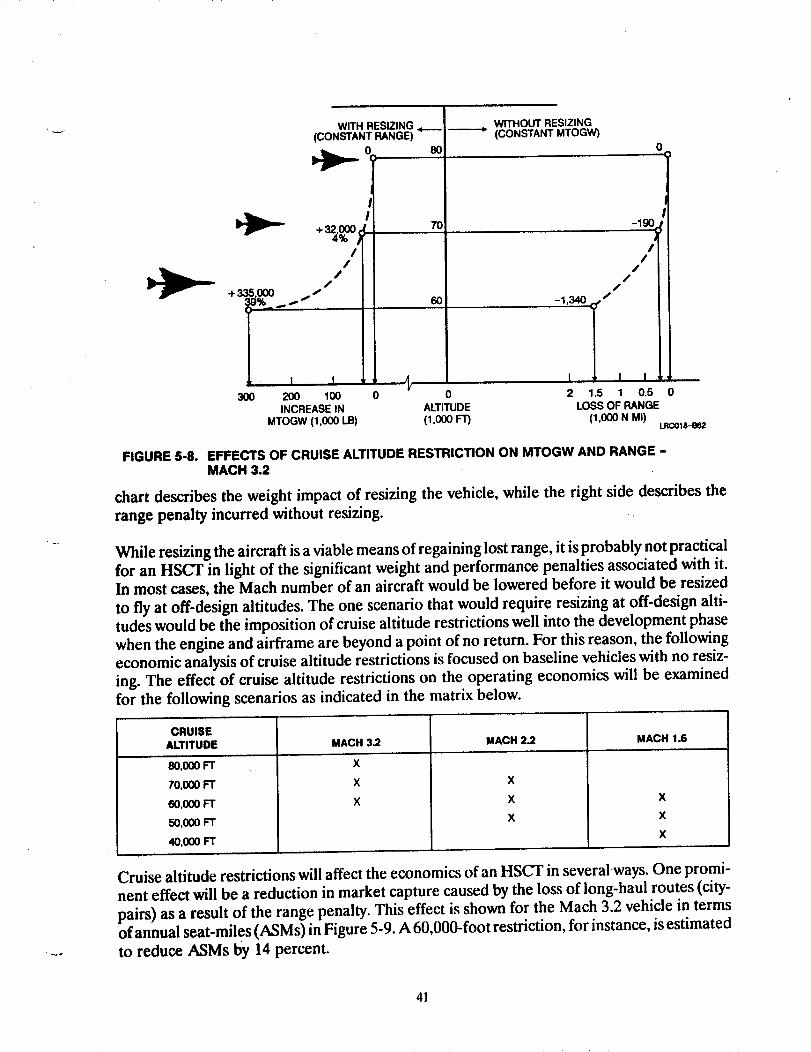
3OO

WITH RESIZING •(CONSTANT RANGE)

II!

+_%ooo,I

//

JS

80

7C

6O

WITHOUT RESIZlNG(CONSTANT MTOGW)

0

III II

JJ

-1.340

I I ' % I I2oo 100 0 0 2 1.S 1 0.5 0INCREASE IN ALTITUDE LOSS OF RANGE

MTOGW (1,000 LB) (1,000 FT) (1,000 N al)LRCO|8-BB2

FIGURE 5-8. EFFECTS OF CRUISE ALTITUDE RESTRICTION ON MTOGW AND RANGE -

MACH 3.2

chart describes the weight impact of resizing the vehicle, while the right side describes the

range penalty incurred without resizing. ..

While resizing the aircraft is a viable means of regaining lost range, it is probably not practical

for an HSCT in light of the significant weight and performance penalties associated with it.

In most cases, the Mach number of an aircraft would be lowered before it would be resized

to fly at off-design altitudes. The one scenario that would require resizing at off-design alti-

tudes would be the imposition of cruise altitude restrictions well into the development phase

when the engine and airframe are beyond a point of no return. For this reason, the following

economic analysis of cruise altitude restrictions is focused on baseline vehicles with no resiz-

ing. The effect of cruise altitude restrictions on the operating economics will be examined

for the following scenarios as indicated in the matrix below.

CRUISEALTITUDE MACH 3.2 MACH 2.2 MACH 1.6

80,000 FT

70.(XX) FT

60,000 FT

50.000 FT

40,000 FT

X

X

X X

X

X

Cruise altitude restrictions will affect the economics of an HSCT in several ways. One promi-

nent effect will be a reduction in market capture caused by the loss of long-haul routes (city-

pairs) as a result of the range penalty. This effect is shown for the Mach 3.2 vehicle in terms

of annual seat-miles (ASMs) in Figure 5-9. A 60,000-foot restriction, for instance, is estimated

to reduce ASMs by 14 percent.

41

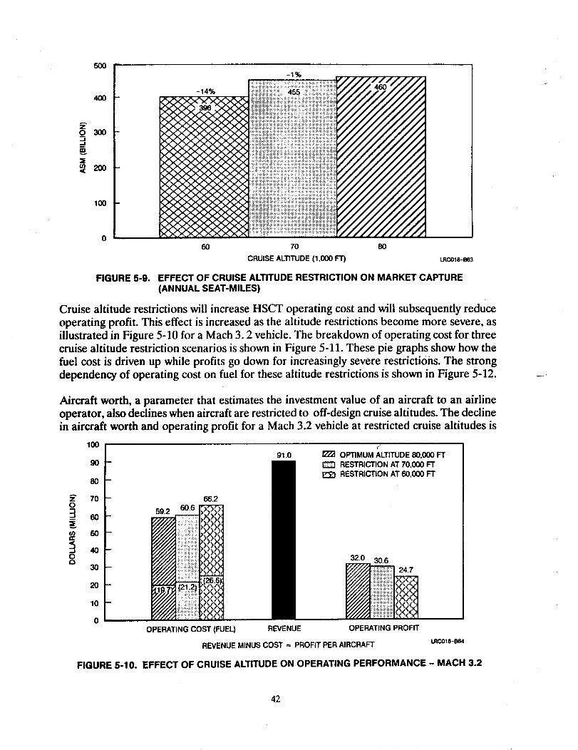
,500

4O0

Azg 3oo.J-J

200

100

-14%

x[_,(X _ X),

IX_K _,( X_Ap

IX _1,( X X X. "J,( _

r,,r,,,_(XX ::,(X),ix_ >KXX Xx)

ix _< x x xx>ix >x_x x',x'">

ix>>(x x >(x:>i),(_ ,_ xx _<x" ),IX), _)<x xx),

KX)< _<_,<>D_>' _<_XX _x),rx">_ _ x x >[_,x),

60

-1%

70 8O

CRUISE ALTITUDE (1,000 FT) LRCO18-B63

FIGURE 5-9. EFFECT OF CRUISE ALTITUDE RESTRICTION ON MARKET CAPTURE

(ANNUAL SEAT-MILES)

Cruise altitude restrictions will increase HSCT operating cost and will subsequently reduce

operating profit. This effect is increased as the altitude restrictions become more severe, as

illustrated in Figure 5-10 for a Mach 3.2 vehicle. The breakdown of operating cost for three

cruise altitude restriction scenarios is shown in Figure 5-11. These pie graphs show how the

fuel cost is driven up while profits go down for increasingly severe restrictions. The strong

dependency of operating cost on fuel for these altitude restrictions is shown in Figure 5-12.

Aircraft worth, a parameter that estimates the investment value of an aircraft to an airline

operator, also declines when aircraft are restricted to off-design cruise altitudes. The decline

in aircraft worth and operating profit for a Mach 3.2 vehicle at restricted cruise altitudes is

100

90

80

700

8

2O

10

0

- 66.2

60.659.2 ,:;._,:_;,,:_

1 . +:.!.'.e ''"J +

::::::::::::::::::::: .., ,', ._>: ,::..::. , ;.

i ' '_'_

91.0d

OPTIMUM ALTITUDE _,000 FI"

RESTRICTION AT 70.(XX) FTRESTRICTION AT 60,000 PT

OPERATING COST (FUEL) REVENUE OPERATING PROFIT

REVENUE MINUS COST = PROFIT PER AIRCRAFT LRCO_e-B84

FIGURE 5-10. EFFECT OF CRUISE ALTITUDE ON OPERATING PERFORMANCE - MACH 3.2

42

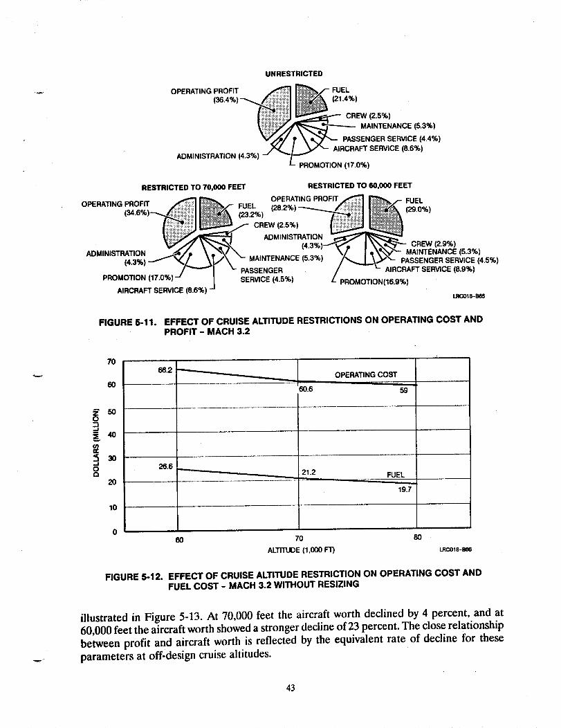
UNRESTRICTED

ADMINISTRATION (4.3%_

,.%f FUEL_:'_. (21.4%)

CREW (2.5%)

o.--..-_...._ MAINTENANCE (5.3%)

PASSENGER SERVICE (4.4%)/_-- AIRCRAFT SERVICE (8.6%)

PROMOTION (17.0%)

RESTRICTED TO 70,000 FEET

OPERATING PROFIT __

(34.6%)___1_

ADMINISTRATION _._/p _ I

(4.3%) "_- _,/.,..._]PROMOTION (17.0%) "J

AIRCRAFT SERVICE (8.6%) -

RESTRICTED TO 60,000 FEET

FUEL OPERATING PROFIT_ _7N % (28.2%)-----.-_4_.l_..:i_ (23.2) L:_i!| l::i3"_i

CREW(2.5%){iii ADMINISTRATION _r_

>X_--MAINTENANCE (5-3% ) y'_.,'_PASSENGER ' 'SERVICE (4.5%)

_.,A/- FUELi!iiN

_CREW 12.9%1_e_%_/__MAINTENANCE (5.3%)J_- PASSENGER SERVICE (4.5%)

AIRCRAFT SERVICE (8.9%)

[ PROMOTION(16.9%)

LRCO18-B85

FIGURE 5-11. EFFECT OF CRUISE ALTITUDE RESTRICTIONS ON OPERATING COST ANDPROFIT - MACH 3.2

70

6O

i" 5OO

=v 4o

O(3

2O

10

66.2

26.6

OPERATING COST

60.6 59

21.2 FUEL

19.7

60 70 80

ALTITUDE (1.06O Fr) LRCO18-B88

FIGURE 5-12. EFFECT OF CRUISE ALTITUDE RESTRICTION ON OPERATING COST ANDFUEL COST - MACH 3.2 WITHOUT RESIZlNG

illustrated in Figure 5-13. At 70,000 feet the aircraft worth declined by 4 percent, and at60,000 feet the aircraft worth showed a stronger decline of 23 percent. The close relationship

between profit and aircraft worth is reflected by the equivalent rate of decline for these

parameters at off-design cruise altitudes.

43

200

180

160

_" 140O

3_ 126

l¢ 100

2=oe_

6O

40

20

148

24.7

184AIRCRAFT WORTH -- 192

30J 32OPERATING PROFIT

6O 70

ALTITUDE (1.000 FT)

8O

LRCO18-B87

FIGURE 5-13. EFFECT OF CRUISE ALTITUDE ON AIRCRAFT WORTH AND OPERATING

PROFIT - MACH 3.2 WITHOUT RESIZlNG

A summary of the economic impact of cruise altitude restrictions is provided in Table 5-3.

Shown are the operating cost, profit, and aircraft worth, with corresponding percentage

changes. Portions of these data are displayed graphically in Figure 5-14. This figure shows

that the expected increase in aircraft worth with increasing Mach number at a design range

of 6,500 nautical miles can be counteracted by altitude restrictions. For instance, the

Mach 2.2 operating profit and aircraft worth exceeds that of the Mach 3.2 aircraft for a

60,000-foot restriction.

5.5 CONCLUSIONS

Results showed that ozone depletion is a function of the cruise Mach number of the air-

craft, primarily because of the strong dependence of ozone impact on injection altitude.

For the P&W turbine bypass engine with a cruise EINOx of approximately 5, the only

configuration that results in ozone depletions in the 1-percent range is the Mach 1.6

TABLE 5-3

AIRCRAFT ECONOMIC PERFORMANCE AT DIFFERENT CRUISE ALTITUDES

CRUISEALTITUDE(1,000 FT)

8O

7O

6O

5O

40

OPERATING COST ($ MILLION)PERCENT OF CHANGE

M3._

59

60.6

66.2

% M2.2 % M1.6 %

+ 2.7 49

+12 50 +2 45

54 +10 46

51

+2

+13

PROFIT ($ MILLION)PERCENT OF CHANGE

M3.2

32

30.6

24.7

% M2.2 % M1.6 %

-4.4 26

-23 25 -4 18

20 J-23 17

12

-6

-33

AIRCRAFT WORTH ($ MILLION)PERCENT OFCHANGE

M3.2

192

184

148

% M2_ % M1.6 %

-4 156

-23 151 -3

125 -20

110

103 -6.4

73 -33

LRC018-B68

44

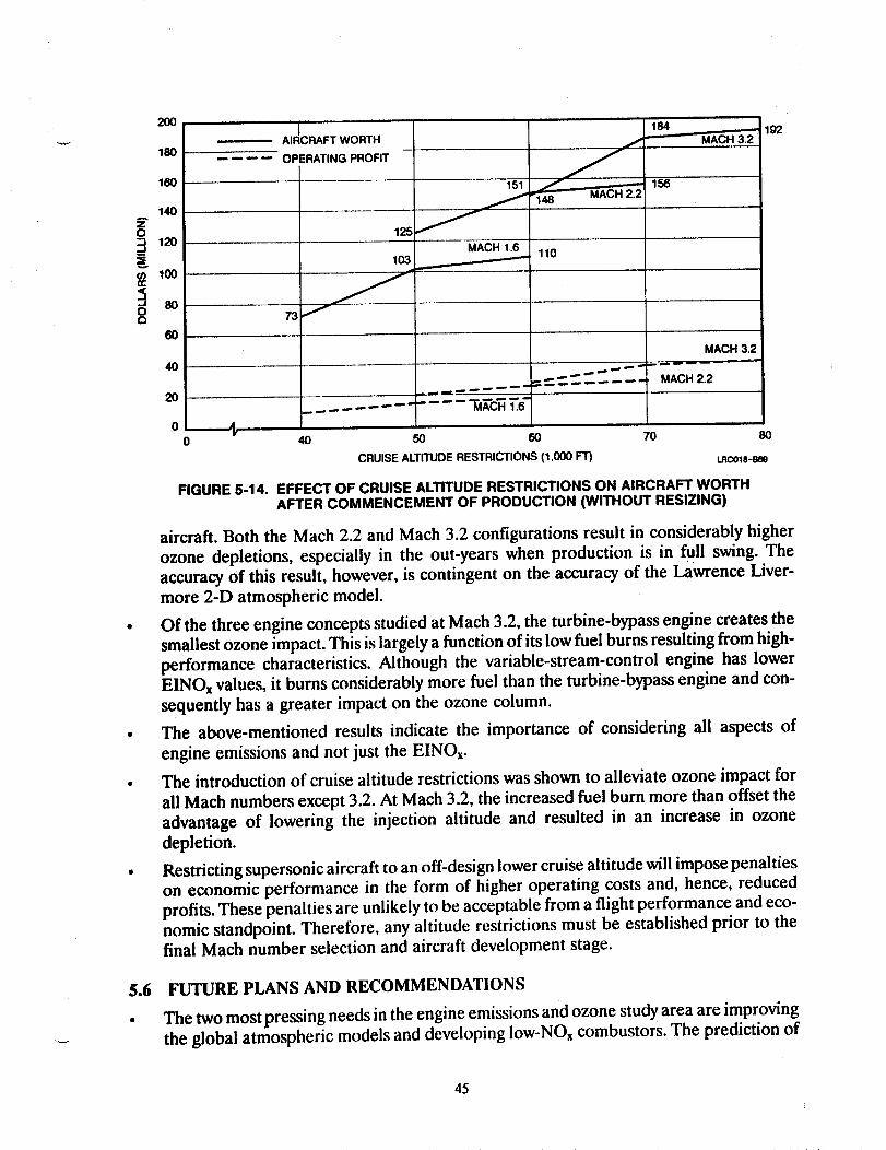
2OO

180

180

140A

n,O

__ 120

100

g60

40

5.6

20

0

151

125 J

103

73 f

MACH 1.6

.... _R_T_

J

184 - 192- MACH 3.2

-- 156

'148 MACH 2.2

110

MACH 3.2

MACH 2.2

40 50 60 70 80

CRUISE ALTITUDE RESTRICTIONS (1,000 FT) LRCOle-Bee

FIGURE 5-1 4. EFFECT OF CRUISE ALTITUDE RESTRICTIONS ON AIRCRAFT WORTHAFTER COMMENCEMENT OF PRODUCTION (WITHOUT RESlZlNG)

aircraft. Both the Mach 2.2 and Mach 3.2 configurations result in considerably higher

ozone depletions, especially in the out-years when production is in full swing. The

accuracy of this result, however, is contingent on the accuracy of the Lawrence Liver-

more 2-D atmospheric model.

Of the three engine concepts studied at Mach 3.2, the turbine-bypass engine creates thesmallest ozone impact. This is largely a function of its low fuel burns resulting from high-

performance characteristics. Although the variable-stream-control engine has lowerEINOx values, it burns considerably more fuel than the turbine-bypass engine and con-

sequently has a greater impact on the ozone column.

The above-mentioned results indicate the importance of considering all aspects of

engine emissions and not just the EINOx.

The introduction of cruise altitude restrictions was shown to alleviate ozone impact for

all Mach numbers except 3.2. At Mach 3.2, the increased fuel burn more than offset the

advantage of lowering the injection altitude and resulted in an increase in ozone

depletion.

Restricting supersonic aircraft to an off-design lower cruise altitude will impose penalties

on economic performance in the form of higher operating costs and, hence, reduced

profits. These penalties are unlikely to be acceptable from a flight performance and eco-

nomic standpoint. Therefore, any altitude restrictions must be established prior to the

final Mach number selection and aircraft development stage.

FUTURE PLANS AND RECOMMENDATIONS

The two most pressing needs in the engine emissions and ozone study area are improving

the global atmospheric models and developing low-NOx combustors. The prediction of

45

annual fuel burns from HSCT fleets can be considered to be a fairly mature process. The

wide variation in ozone concentration results from the various atmospheric models

clearly needs to be addressed before the intricacies of fleet sizes, flight paths, etc. can

be meaningfully addressed by the aifframers.

There is an urgent need for well-defined emissions criteria. Trade studies, such as those

conducted in this study, are valuable inasmuch as they can identify trends and rule out

scenarios that are clearly unacceptable. However, before the final design and Mach num-

ber selection for an HSCT can be made, emissions criteria must be defined so that costly

redesigns and delays can be avoided.

Three-dimensional atmospheric models may become an industry standard if their

accuracy proves to be superior to two-dimensional models and the computer costs are

not excessive. To support three-dimensional models, it will be necessary to revamp cur-

rent methodologies for generating global scenarios.

It would be mutually beneficial if a standardized methodology and format were defined

and followed by industry and university researchers.

Current HSCT emissions scenarios do not adequately account for the effect of the sub-

sonic fleet. This can be misleading with regard to data interpretation and may be causing

significant error in the overall ozone results. The optimum solution to this problem

would be for the airframers to agree on a representative subsonic fleet for the time

period in question, and then include these emissions in the total HSCT predictions.

Along with the commercial subsonic fleet, prediction accuracy would be improved by

including military flights. Difficulties arise when eastern European countries are brought

into consideration because flight data are difficult to obtain. Some effort, however,

should be made to incorporate as much of the current aviation activity as possible so that

sound decisions regarding engine emissions can be made for both supersonic and sub-sonic aircraft.

The impact of traffic seasonality should be included in the development of engine emis-

sions scenarios. The global transport and atmospheric chemistry have a seasonal depend-

enee, as does the air traffic. These factors need to be addressed to determine their impacton overall ozone concentration results.

Certain routes have the potential to be rerouted to avoid flights through regions that are

thought to be particularly sensitive to ozone depletion. For example, transatlantic flights

might be rerouted away from the typical polar routes if this proved to be beneficial from

an ozone standpoint. Alternative emissions scenarios simulating these types of rerouting

can be developed and sent to global modelers for assessment.

46

SECTION 6

CONCLUSIONS

Following are conclusions drawn from the system studies in the environmental, marketing,

economic, and emission impact areas:

Long-term prospects for international passenger traffic gains are good. Supersonic

traffic demands are promising.

World demands for new passenger aircraft, including supersonic transports, are showing

healthy growth. HSCT projections for the year 2025 could total 2,300 aircraft. However,accurate HSCT fleet forecasts will require a better understanding of many complex

factors such as elasticity, stimulation, fare premium, and supersonic cruise overland

restrictions.

Supersonic operation may introduce major changes to the current global route structureto avoid overland flights. With creative rerouting, some supersonic network scenarios

show good potential of capturing half the long-range markets.

The atmospheric impact model results of vertical ozone depletion show a significant

dependence on cruise injection altitude.

Ozone depletion is significantly less with the Mach 1.6 configuration than with the

Mach 2.2 and Mach 3.2 configurations for a given combustion technology.

The introduction of cruise altitude restrictions after production implementation allevi-

ates ozone impact for all Mach numbers except 3.2. At Mach 3.2, the increased fuel burn

more than offset the advantage of lowering the injection altitude and resulted in an

increase in ozone depletion.

Restricting supersonic aircraft to an off-design lower cruise altitude will impose penalties

on economic performance in the form of higher operating costs and, hence, reduced air-

line operating profits. The penalties are unlikely to be acceptable from a flight perform-

ance economic standpoint. Therefore, any altitude restrictions must be established prior

to final Mach number selection in the aircraft development stage.

47

SECTION 7

RECOMMENDATIONS

Following are the recommendations for the environmental, marketing, economic, and emis-

sion impact areas:

Continue market and economic analysis of HSCT commercial value and economics,

considering fuel prices, operational procedures, dispatch reliability, and environmental

concerns.

Continue parametric studies of different design ranges and passenger configurations to

optimize the HSCT's economic viability.

Continue supersonic network research on ways to respond to environmental concerns,

operational policies, marketing strategies, and airline requirements.

Continue to assess the effect of these supersonic network scenarios on aircraft economic

performance, productivity, and fleet projections.

In atmospheric emission impact, continue Mach number trade studies after (1) two-

dimensional atmospheric models have been updated to include fine grid densities and

the effects of heterogeneous chemistry and (2) the city-pair network has been updated.

Use three-dimensional atmospheric models for baseline atmospheric impact scenarios

and compare the results to the two-dimensional model data.

Future effects of HSCT operation on ozone depletion should include the effects of the

subsonic fleet in the atmosphere for an appropriate year (e.g., 2015).

Consider the effects of including additional subsonic operation (e.g., military, USSR,

China, cargo, and turboprop).

Evaluate the effects of traffic seasonality on atmospheric effects.

Develop alternative emission scenarios to avoid routes having high sensitivity to ozone

depletion (e.g., rerouting of polar routes).

49

APPENDIX ABASIC TRAFFIC DATA BASE

250 CITY-PAIRS

IN DESCENDING ORDER OF

SCHEDULED SEATS

' LRC018-80

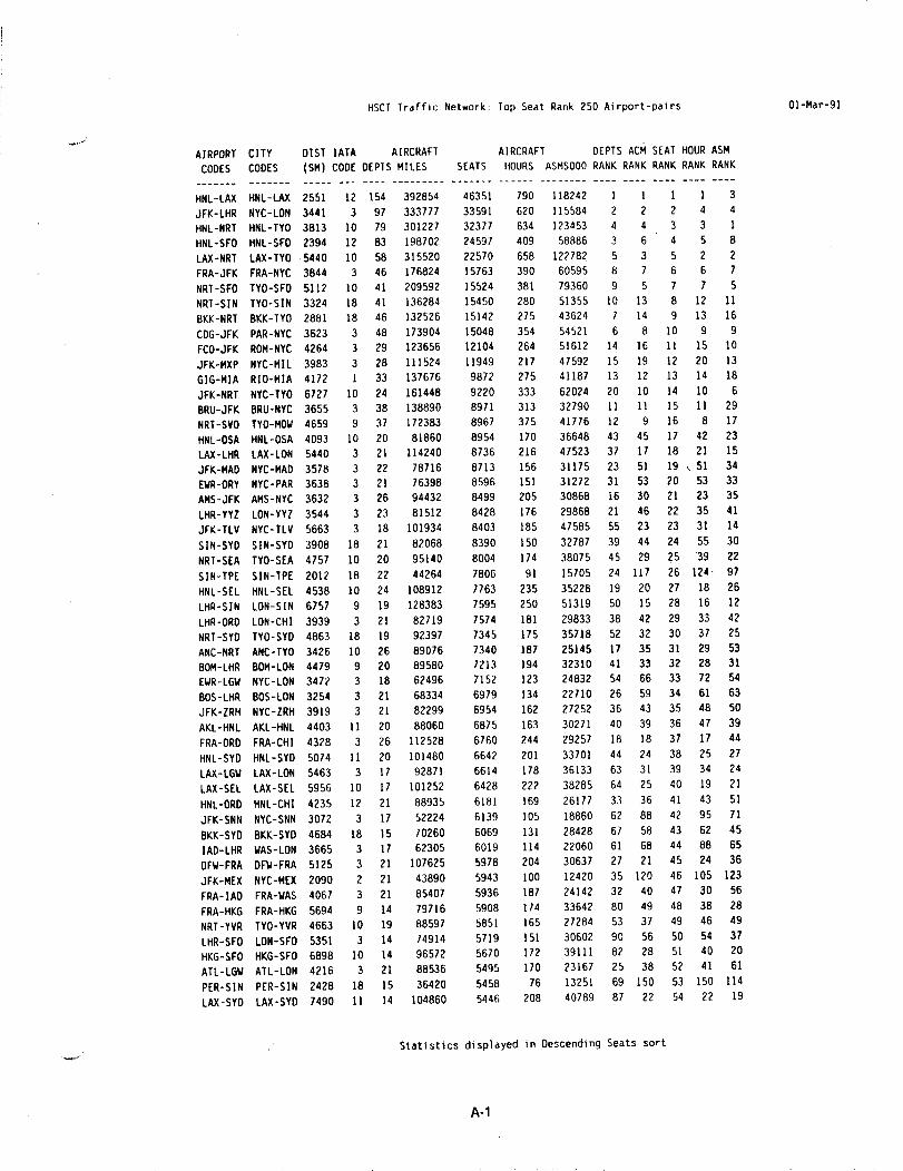
HSCI Traffic Network: Top Seat Rank 250 Airport-pairs 01-Mar-9]

AIRPORT CITY

CODES CODES

HNL-LAX HNL-LAX 2551 12 154 392854

JFK-LHR NYC-LON 3441 3 97 333777

HNL-NRT HNL-TYO 3813 10 79 301227

HNL-SFO HNL-SFO 2394 ]2 83 198702

LAX-NRT LAX-TYO 5440 10 58 315520

FRA-JFK FRA-NYC 3844 3 46 176824

NRT-SFO TYO-SFO 5]]2 10 41 209592

NRI-SIN TYO-SIN 3324 18 41 136284

BKK-NRT BKK-TYO 2881 18 46 132526

CDG-JFK PAR-NYC 3623 3 48 173904

FCO-JFK ROM-NYC 4264 3 29 123656

JFK-MXP NYC-MIL 3983 3 28 111524

GIG-MIA RIO-MIA 4172 I 33 137676

JFK-NRT NYC-TYO 6727 I0 24 161448

BRU-JFK BRU-NYC 3655 3 38 138890

NRT-SVO TYO-MOW 4659 9 37 172383

HNL-OSA HNL-OSA 4093 10 20 81860

LAX-LHR LAX-LON 5440 3 21 114240

JFK-MAD NYC-MAD 3578 3 22 18716

EWR-ORY NYC-PAR 3638 3 21 76398

AMS-JFK AMS-NYC 3632 3 26 94432

LHR-YYZ LON-YYZ 3544 3 23 81512

JFK-TLV NYC-TLV 5663 3 18 101934

SIN-SYD SIN-SYD 3908 18 21 82068

NRT-SEA TYO-SEA 4751 10 20 95140

SIN-TPE SIN-TPE 2012 18 22 44264

HNL-SEL HNL-SEL 4538 IO 24 108912

LHR-SIN LON-SIN 6757 9 ]9 128383

LHR-ORD LON-CHI 3939 3 21 82719

NRT-SYD TYO-SYD 4863 18 19 92397

ANC-NRT ANC-TYO 3426 10 26 89076

BOM-LHR BOM-LON 4479 9 20 89580

EWR-LGW NYC-LON 3472 3 ]8 62496

BOS-LHR BOS-LON 3254 3 21 68334

JFK-ZRH NYC-ZRH 3919 3 21 82299

AKL-HNL AKL-HNL 4403 II 20 88060

FRA-ORD FRA-CHI 4328 3 26 112528

HNL-SYD HNL-SYD 5074 II 20 101480

LAX-LGW LAX-LON 5463 3 17 92871

LAX-SEL LAX-SEL 5956 10 17 101252

HNL-ORD HNL-CHI 4235 12 21 88935

JFK-SNN NYC-SNN 3072 3 II 52224

BKK-SYD BKK-SYD 4684 18 15 70260

IAD-LHR WAS-LON 3665 3 11 62305

DFW-FRA DFW-FRA 5125 3 21 107625

JFK-MEX NYC-MEX 2090 2 21 43890

FRA-IAD FRA-WAS 4067 3 21 85407

FRA-HKG FRA-HKG 5694 9 14 79716

NRT-YVR TYO-YVR 4663 I0 19 88597

LHR-SFO LON-SFO 5351 3 14 14914

HKG-SFO HKG-SFO 6898 10 14 96572

ATL-L6W ATL-LON 4216 3 21 88536

PER-SIN PER-SIN 2428 18 15 36420

LAX-SYD LAX-SYD 7490 11 14 104860

DIST IATA AIRCRAFT AIRCRAFT DEPTS ACM SEAT HOUR ASM

(SM) CODE DEPIS MILES SEATS HOURS ASMSO00 RANK RANK RANK RANK RANK

..............................................................

46351

33591

32377

24597

22570

15763

15524

15450

15142

15048

12104

11949

9872

9220

8971

8967

790 118242 I I I I 3

620 115584 2 2 2 4 4

634 123453 4 4 3 3 1

409 58886 3 6 4 5 8

658 122782 5 3 5 2 2

390 60595 8 7 6 6 7

381 79360 9 5 7 7 5

280 51355 I0 13 8 12 11

275 43624 7 14 9 13 16

354 54521 6 8 I0 9 9

264 51612 14 16 II 15 lO

217 47592 15 19 12 20 13

275 41187 13 12 13 14 18

333 62024 20 10 14 I0 6

313 32790 11 11 15 ll 29

375 41776 12 9 16 8 17

8954 170 36648 43 45 i1 42 23

8736 216 47523 37 ll 18 21 15

8713 156 31175 23 51 19 _ 51 34

8596 151 31272 31 53 20 53 33

8499 205 30868 16 30 21 23 35

8428 176 29868 21 46 22 35 41

8403 185 47585 55 23 23 31 14

8390 150 32787 39 44 24 55 30

8004 174 38075 45 29 25 39 22

7806 9] 15705 24 117 26 ]24 97

7763 235 35228 19 20 27 18 26

7595 250 51319 50 15 28 16 12

1574 181 29833 38 42 29 33 42

7345 175 35718 52 32 30 37 25

7340 187 25145 17 35 31 29 53

7213 194 32310 41 33 32 28 31

7152 123 24832 54 66 33 72 54

6979 134 22710 26 59 34 61 63

6954 162 27252 36 43 35 48 50

6875 163 30271 40 39 36 47 39

6760 244 29257 18 18 37 17 44

6642 201 3370] 44 24 38 25 27

6614 178 36133 63 31 39 34 24

6428 222 38285 64 25 40 19 21

6181 169 26177 33 36 41 43 51

6139 105 18860 62 88 42 95 71

6069 131 28428 67 58 43 62 45

6019 114 22060 61 68 44 88 65

5978 204 30637 27 21 45 24 36

5943 100 12420 35 120 46 105 123

5936 187 24142 32 40 47 30 56

5908 174 33642 80 49 48 38 28

5851 165 27284 53 37 49 46 49

5719 151 30602 90 56 50 54 37

5670 172 39111 82 28 51 40 20

5495 170 23167 25 38 52 41 61

5458 76 13251 69 150 53 150 114

5446 208 40789 87 22 54 22 19

Statistics displayed in Descending Seats sort

A-I

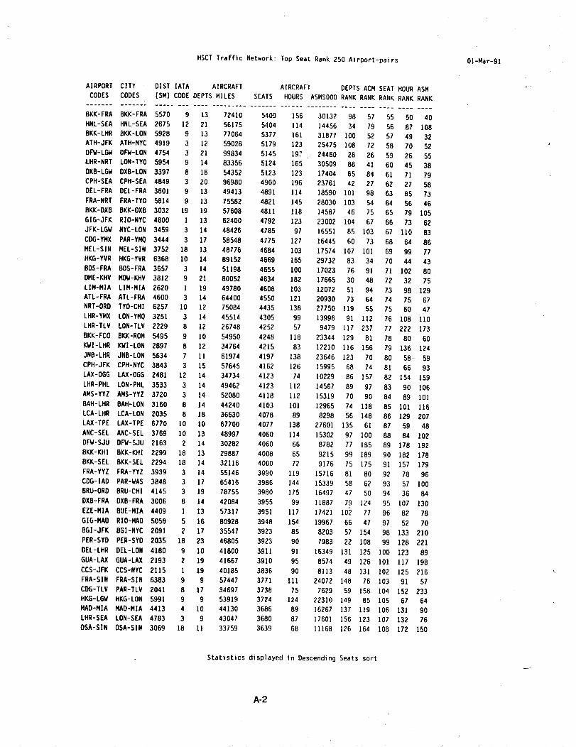
HSCT Traffic Network: Top Seat Rank 250 Airport-pairs OI-Mar-91

AIRPORT CITY - DIST IATA AIRCRAFT AIRCRAFT DEPTS ACM SEAT HOUR ASM

CODES CODES (SM) CODE DEPTS MILES SEATS HOURS ASMSO00 RANK RANK RANK RANK RANK

............................................................................

BKK-FRA 8KK-FRA 5570 9 13 72410 5409 156 30132 98 57 55 50 40

HNL-SEA HNL-SEA 2675 12 2] 56175

BKK-LHR BKK-LON 5928 9 13 77064

ATH-JFK ATH-NYC 4919 3 12 59028

DF'W-LGW DFW-LON 4754 3 21 99834

LHR-NRT LON-TYO 5954 9 14 83356

DXB-LGW DXB-LON 3397 8 16 54352

CPH-SEA CPH-SEA 4849 3 20 96980

DEL-FRA DEL-FRA 3801 9 13 49413

FRA-NRT FRA-TYO 5814 9 13 75582

BKK-DXB BKK-DXB 3032 19 19 57608

GIG-JFK RIO-NYC 4800 I 13 62400

JFK-LGW NYC-LON 3459 3 14 48426

CDG-YMX PAR-YMQ 3444 3 17 58548

MEL-SIN MEL-SIN 3752 18 13 48776

HKG-YVR HKG-YVR 6368 10 14 89152

BOS-FRA 80S-FRA 3657 3 14 51198

DME-KHV MOW-KHV 3812 9 21 80052

LIM-MIA LIM-MIA 2620 1 19 49780

ATL-FRA ATL-FRA 4600 3 ]4 64400

NRT-ORD TYO-CHI 6257 IO 12 75084

LHR-YMX LON-YMQ 3251 3 14 45514

LHR-TLV LON-TLV 2229 8 12 26748

BKK-FCO BKK-ROM 5495 9 10 54950

KWI-LHR KWI-LON 2897 8 12 34764

JNB-LHR JNB-LON 5634 7 11 61974

CPH-JFK CPH-NYC 3843 3 15 57645

LAX-OGG LAX-OGG 2481 12 14 34734

LHR-PHL LON-PHL 3533 3 14 49462

AMS-YYZ AMS-YYZ 3720 3 14 52080

BAH-LHR BAH-LON 3160 8 14 44240

LCA-LHR LCA-LON 2035 8 18 36630

LAX-TPE LAX-TPE 6770 IO 10 67700

ANC-SEL ANC-SEL 3769 10 13 48997

OFW-SJU DFW-SJU 2163 2 14 30282

BKK-KHI BKK-KHI 2299 18 13 29887

8KK-SEL 6KK-SEL 2294 18 14 32116

FRA-YYZ FRA-YYZ 3939 3 14 55146

COG-IAD PAR-WAS 3848 3 17 654]6

BRU-ORD 8RU-CHI 4]45 3 19 78755

DXB-FRA OXB-FRA 3006 8 14 42084

EZE-MIA BUE-MIA 4409 ] 13 573]7

GIG-HAD RIO-HAD 5058 5 16 80928

BGI-JFK BGI-NYC 2091 2 17 35547

PER-SYD PER-SYD 2035 18 23 46805

DEL-LHR DEL-LON 4180 9 10 41800

6UA-LAX GUA-LAX 2]93 2 19 4]667

CCS-JFK CCS-NYC 2115 l 19 40185

FRA-SIN FRA-SIN 6383 9 9 57447

CDG-TLV PAR-TLV 2041 8 17 34697

HKG-LGW HKG-LON 5991 9 9 53919

MAD-M]A MAD-MIA 4413 4 lO 44130

LHR-SEA LON-SEA 4783 3 9 43047

OSA-SIN OSA-SIN 3069 18 11 33759

5404

5377

5179

5145

5124

5123

4900

4891

4821

4811

4792

4785

4775

4684

4669

4655

4634

4608

4550

4435

4305

4252

4248

4215

4]97

4162

4123

4123

4118

4103

4078

4077

4060

4060

4O08

4000

3990

3986

3980

3955

3951

3948

3923

3923

3911

39]0

3836

3771

3738

3724

3686

3680

3639

114 14456 34 79 56 87 108

161 31877 lO0 52 57 49 32

123 25475 108 72 58 70 52

197 24460 28 26 59 26 55

165 30509 88 41 60 45 38

]23 ]7404 65 84 61 71 79

196 23761 42 27 62 27 58

114 18590 10] 98 63 85 73

145 28030 103 54 64 56 46

118 14587 46 75 65 79 105

123 23002 104 67 66 73 62

97 16551 85 103 67 II0 83

]27 16445 60 73 68 64 86

I03 17574 TO/ lOl 69 99 17

165 29732 83 34 70 44 43

IO0 17023 76 91 71 102 80

182 17665 30 48 72 32 75

103 12072 51 94 73 98 129

121 20930 73 64 14 75 67

138 27750 119 55 75 60 47

99 13996 91 112 76 108 110

57 9479 117 237 77 222 173

118 23344 129 81 78 80 60

83 12210 116 156 79 136 124

138 23646 123 70 80 58" 59

126 15995 68 74 8I 66 93

74 10229 86 157 82 154 159

ll2 14567 89 97 83 90 106

112 15319 70 90 84 89 101

101 12965 74 118 85 I01 I16

89 8298 56 148 86 129 207

138 27601 135 61 87 59 48

1]4 15302 97 100 88 84 102

66 8782 77 185 89 178 192

65 9215 99 189 90 182 178

12 9176 15 175 91 157 179

119 15716 81 80 92 78 96

144 15339 58 62 93 57 IO0

175 16497 47 50 94 36 84

99 11887 79 ]24 95 107 130

117 1742!1 102 71 96 82 78

154 19967 66 47 97 52 70

85 8203 57 154 98 133 210

90 7983 22 108 99 128 221

91 16349 131 125 ]OO 123 89

95 8574 49 126 lO] 117 198

90 8113 48 131 102 125 216

III 24072 148 16 ]03 91 57

75 7629 59 158 104 152 233

124 22310 149 85 105 67 64

89 I6267 137 ]19 106 131 90

87 17601 156 123 107 132 76

68 11168 126 164 108 172 150

Statistics displayed in Descending Seats sort

A-2

HSCT Iraffic Network: Top Seat Rank 250 Airport-pairs 01-Mar-g1

L

AIRPORT CITY DIST ]ATA AIRCRAFT AIRCRAFT OEPTS ACM SEAT HOUR ASM

CODES CODES (SM) CODE DEPTS MILES SEATS HOURS ASMSO00 RANK RANK RANK RANK RANK

.......................................... ..................................

AMS-ATL AMS-ATL 4388 3 13 57044

IAH-LGW HOU-LON 4840 3 14 67760

DME-IKT MOW-]KT 2604 9 21 54684

CDG-NRT PAR-TYO 6027 9 lO 60270

OGG-SFO OGG-SFO 2335 12 14 32690

DXB-KUL DXB-KUL 3434 19 12 41208

BOM-SIN BOM-SIN 2435 18 12 29220

BOM-FRA BOM-FRA 4079 9 9 36711

HNL-LAS HNL-LAS 2757 12 9 24813

LHR-NBO LON-NBO 4248 7 9 38232

ORD-ZRH CHI-ZRH 4428 3 14 61992

]AO-NRT WAS-TYO 6736 10 6 40416

JED-LHR JED-LON 2960 8 9 26640

HNL-MNL HNL-MNL 5290 10 9 47610

JFK-LIS NYC-LIS 3357 3 12 40284

AKL-LAX AKL-LAX 6512 11 8 52096

ORD-SJU CHI-SJU 2072 2 14 29008

CVG-ORY CVG-PAR 4]44 3 12 49728

HNL-IAH HNL-HOU 3896 12 7 27272

AUH-SIN AUH-SIN 3672 19 8 29376

HNL-STL HNL-STL 4120 ]2 7 28840

BKK-CPH BKK-CPH 5344 9 ]0 53440

LGW-MIA LON-MIA 4429 4 11 48719

CDG-FDF PAR-FDF 4266 4 8 34128

ATH-SIN ATH-SIN 5626 9 7 39382

ARN-JFK STO-NYC 3908 3 14 54712

COG-LAX PAR-LAX 5652 3 9 50868

FRA-JNB FRA-JNB 5396 l 8 43168

HKG-SEA HKG-SEA 6474 10 lO 64740

DTW-NRT DTT-TYO 6380 ]0 7 44660

BAH-HKG BAH-HKG 3978 19 7 27846

BAH-LGW BAH-LON 3144 8 7 22008

GUM-HNL GUM-HNL 3797 ]0 13 49361

LHR-MIA LON-MIA 4414 4 l 30898

AMS-LAX AMS-LAX 5562 3 8 44496

JFK-MUC NYC-MUC 4028 3 13 52364

BOS-SNN BOS-SNN 2885 3 7 20195

BOS-LGW 80S-LON 3272 3 7 22904

LGW-MSP LON-MSP 4022 3 7 • 28154

OSA-SFO OSA-SFO 5374 ]0 l 37618

SEA-SEL SEA-SEL 5180 lO l 36260

DEL-SIN DEL-SIN 2582 18 8 20656

CDG-MIA PAR-MIA 4577 4 8 36616

CGK-NRT JKT-TYO 3623 18 7 25361

HNL-NAN HNL-NAN 3171 II 9 28539

AMS-ORD AMS-CHI 4106 3 8 32848

LHR-YVR LON-YVR 4707 3 10 47070

LGW-NRT LON-TYO 5967 9 6 35802

JFK-WAW NYC-WAW 4253 3 11 46783

FRA-SFO FRA-SFO 5681 3 l 39767

DUS-ORD DUS-CHI 4214 3 12 50568

HEL-JFK HEL-NYC 4103 3 II 45133

JFK-ORY NYC-PAR 3623 3 ]0 36230

BCN-JFK BCN-NYC 3820 3 12 45840

3611 123 15845 96 78 109 68 95

3500 127 16940 84 60 110 65 81

3444 120 8967 29 83 111 76 187

3435 118 20703 130 71 112 81 68

3409 66 7960 92 173 113 180 222

3366 84 11558 114 127 114 134 134

3359 60 8179 llO 199 115 203 213

3288 80 13412 141 147 116 141 I12

3243 50 8941 150 257 117 262 189

3235 79 13742 155 143 118 146 111

3172 123 14047 94 69 119 74 109

3168 84 21340 299 129 120 135 66

3142 58 9298 153 241 121 218 175

3138 90 16599 151 104 122 127 82

3109 81 10437 115 130 123 138 157

3093 96 20141 157 89 124 111 69

3080 65 6382 93 204 125 187 279

3048 100 12631 112 96 126 103 119

3038 49 11836 243 229 127 264 132

3018 56 11082 162 198 128 223 IS1

3017 55 12430 247 208 129 234 122

3010 115 16085 128 86 130 83 92

3001 109 13292 124 102 131 94 113

2957 72 12614 164 162 132 158 121

2928 77 16473 184 134 133 149 85

2920 123 11412 72 82 134 69 141

2903 102 16408 ]45 92 135 100 87

2901 96 15653 168 122 136 114 98

2901 120 18781 133 63 137 77 72

2900 93 18502 226 115 138 120 74

2884 56 11473 189 222 139 224 138

2884 48 9067 190 283 140 266 183

2884 94 10950 105 99 141 118 153

2884 65 12730 257 180 142 186 118

2864 92 15930 160 116 143 121 94

2837 104 I1427 106 87 144 96 139

2807 40 8099 197 300 145 304 218

2800 46 9162 196 275 ]46 281 180

2800 63 I1262 255 219 147 194 146

2800 68 ]5047 265 144 148 171 104

2800 80 14504 267 151 149 143 107

2793 42 72li 166 295 150 299 248

2758 78 12624 165 149 151 147 120

2730 51 9891 207 253 152 256 165

2730 58 8657 152 213 153 217 196

2724 69 11185 161 169 154 165 149

2713 94 12770 136 105 155 119 117

2706 72 16]48 304 153 156 159 91

2700 96 ]1482 122 ]09 157 116 136

2667 80 15151 236 133 158 142 103

2665 110 11230 113 93 159 92 148

2665 lO0 10935 120 113 160 104 154

2625 74 9510 134 152 161 153 170

2618 I03 I0001 109 111 162 97 163

Statistics displayed in Descendlng Seats sort

A-3

HSCT Traffic Network: lop Seat Rank 250 Airport-pairs OI-Mar-9I

AIRPORT CITY DIST IATA AIRCRAFT AIRCRAFI DEPTS ACM SEAT HOUR ASM

CODES CODES (SM) CODE DEPIS MILES SEATS HOURS ASMSOOO RANK RANK RANK RANK RANK

............................................................................

CMB-DXB CMB-DXB 2043 19

CDG-PTP PAR-PTP 4204 4

AMS-YMX AMS-YMQ 3429 3

BAH-FRA BAH-FRA 2755 8

KUL-HEL KUL-MEL 3946 18

SFO-TPE SFO-TPE 6439 ]0

DEN-HNL DEN-HNL 3347 12

AKL-SIN AKL-SIN 5222 18

MEL-NAN MEL-NAN 2401 18

EZE-MAD BUE-MAD 6257 5

HKG-SYD HKG-SYD 4581 18

KHV-VKO KHV-MOW 3823 9

LED-TAS LED-TAS 2102 9

UUS-VKO UUS-MOW 4146 9

HKG-MEL HKG-MEL 4601 18

AUH-CGK AUH-JKT 4101 19

BRU-YMX 8RU-YMQ 3461 3

BOS-CD6 BOS-PAR 3436 3

CCS-MAD CCS-MAD 4349 4

AMS-DXB AHS-OXB 3208 8

AMS-AUA AMS-AUA 4893 4

PEK-SHJ BJS-SHJ 3609 19

FRA-PEK FRA-BJS 4836 9

KHI-PEK KHI-BJS 3003 18

BOS-ZRH BOS-ZRH 3732 3

LGW-YYZ LON-YYZ 3564 3

AMS-IAH AMS-HOU 4998 3

DME-HTA MOW-HTA 2937 9

UUD-VKO UUD-MOW 2758 9

HNL-PHX HNL-PHX 2910 12

FRA-M]A FRA-MIA 4820 4

DXB-MNL DXB-MNL 4290 19

EWR-LHR NYC-LON 3454 3

JFK-MAN NYC-MAN 3330 3

HAV-YQX HAV-YQX 2345 2

8KK-OSA BKK-OSA 2601 ]8

CNS-NRT CNS-TYO 3653 18

AKL-NRT AKL-TYO 5490 18

GVA-JFK GVA-NYC 3852 3

JIB-RUN JIB-RUN 2392 16

KUL-NRT KUL-TYO 3337 18

MAD-MEX MAD-MEX 563] 4

HNL-SAN HNL-SAN 2609 12

DXB-ZRH DXB-ZRH 2959 8

FRA-YMX FRA-YMQ 3647 3

FCO-GI6 ROM-RIO 5694 5

MIA-SCL MIA-SCL 4146 I

BOG-JFK BOG-NYC 2481 1

HNL-SJC HNL-SJC 2413 12

DXB-HKG DXB-HKG 3694 ]9

HKG-LHR HKG-LON 5989 9

CAI-LHR CAI-LON 2192 8

HNL-NGO HNL-NGO 4006 10

AMS-DHA AMS-DHA 2946 8

12 24516 2610 52

7 29428 2583 56

7 24003 2576 51

9 24795 2559 54

6 23676 2559 45

10 64390 2544 131

10 33470 2530 70

9 46998 2525 96

8 19208 2516 39

6 37542 2487 69

6 27486 2480 54

7 26761 2450 79

7 14714 2450 34

7 29022 2450 100

6 27606 2442 54

7 28707 2414 55

9 31149 2409 67

9 30924 2404 59

9 39141 2398 75

7 22456 2384 48

8 39144 2362 80

8 28872 2345 71

6 29016 2343 59

9 27027 2325 59

1 26124 2319 49

11 39204 2299 89

7 34986 2296 72

I4 41118 2296 114

14 38612 2296 110

6 17460 2286 34

9 43380 2277 90

6 25740 2256 52

7 24]78 2240 47

7 23310 2240 47

7 16415 2212 34

7 18207 2209 36

6 21918 2206 42

6 32940 2202 66

7 26964 2]96 58

5 11960 2179 25

8 26696 2156 53

5 28155 2150 55

l 18263 2114 36

6 17754 2113 39

7 25529 2071 56

5 28470 2063 58

12 49752 2037 98

7 17367 2030 39

7 16891 2030 35

5 18470 2025 36

5 29945 2025 lO

8 17536 2024 40

4 16024 2024 33

6 17676 20]5 36

5332 111 260 163 252 321

10858 203 197 164 226 155

8834 181 266 165 255 191

7051 140 258 166 238 255

10097 302 268 167 288 161

16381 138 65 168 63 88

8468 132 167 169 163 199

13184 139 107 170 112 115

6040 173 311 171 322 290

15564 290 145 172 168 99

11361 297 227 173 243 144

9366 251 236 174 145 174

5150 254 391 175 367 331

10158 269 202 176 106 160

11238 296 226 177 242 147

9897 188 212 178 230 164

8338 143 178 179 173 205

8260 142 179 180 208 208

10429 144 139 181 151 158

7648 177 279 182 265 231

11556 158 138 183 140 135

8464 174 207 184 162 200

11331 292 203 185 209 145

6983 154 230 186 212 257

8654 198 244 187 263 197

8194 125 137 188 130 211

11475 178 155 189 156 137

6744 78 128 190 86 266

6332 95 141 191 93 280

6652 298 341 192 366 269

10976 147 121 193 126 152

9678 288 245 194 253 167

7737 231 263 195 275 229

7459 248 271 196 278 240

5187 242 362 197 364 330

5747 191 327 198 336 302

8060 283 284 199 298 219

12090 270 168 200 177 128

8459 240 233 201 216 201

5213 341 449 202 447 328

7195 172 238 203 249 249

12107 347 218 204 236 127

5515 245 325 205 345 309

6251 289 334 206 316 283

7553 238 250 207 227 235

11748 327 214 208 215 133

8443 118 95 209 109 202

5036 193 346 210 314 339

4898 246 354 211 359 349

7480 326 322 212 341 238

12129 335 187 213 164 126

4431 163 339 214 305 371

8108 403 369 215 368 211

5937 273 335 216 333 294

Statistics dlsplayed in Descending Seats sort

A-4

HSCT Traffic Network: Top Seat Rank 250 Airport-pairs OI-Mar-91

AIRPORT CITY DIST IAIA AIRCRAFT AIRCRAFT DEPTS ACM SEAT HOUR ASM

CODES CODES (5M) CODE DEPTS MILES SEATS HOURS ASMSO00 RANK RANK RANK RANK RANK

............................................................................

DUS-LAX DUS-LAX 5671 3 6 34026

BOH-HKG BOH-HKG 2670 I8 6 ]6020

AMS-BO5 AMS-BOS 3445 3 7 24115

BOS-GLA BOS-GLA 3020 3 7 21140

CDG-DTW PAR°DTT 3948 3 7 27636

DTW-FRA DTT-FRA 4147 3 l 29029

JFK-VIE NYC-VIE 4224 3 II 46464

ANC-SFO ANC-SFO 2014 12 14 28196

HNL-RUH HNL-RUH 4831 19 5 24155

CAI-LGW CAI-LON 2171 8 6 13026

FRA-GIG FRA-RIO 5942 5 5 29710

AMS-PBM AMS-PBM 4674 4 7 32718

FDF,ORY FDF-PAR 4255 4 4 17020

ORY-PTP PAR-PTP 4193 4 4 16772

HND-HNL TYO-HNL 3845 10 5 19225

LHR-RUH LON-RUH 3080 8 6 18480

OEL-FCO OEL-ROM 3685 9 6 22110

LAX-PPT LAX-PPT 4105 11 6 24630

ATL-HUC ATL-MUC 4786 3 7 33502

BNE-NRT BNE-TYO 4472 18 6 26832

CVG-FRA CVG°FRA 4347 3 7 30429

CVG-LGW CVG-LON 3969 3 7 27783

NRT-PDX TYO-PDX 4810 10 7 33670

POX-SEL POX-SEL 5252 IO 7 36764

DUS-JFK DUS-NYC 3736 3 8 29888

BOS-6RU BOS-BRU 3468 3 6 20808

JFK-SVO NYC-MOW 4646 3 5 23230

KHG-SHA KHG-SHA 2592 18 7 18144

MAD-SDQ MAD-SDQ 4154 4 7 29078

GIG-LHR RIO-LON 5746 5 5 28730

FRA-YVR FRA-YVR 5007 3 8 40056

FRA-THR FRA-THR 2339 8 7 16373

DPS-HEL DPS-MEL 2726 18 7 19082

DTW-SEL DTT-SEL 6603 10 4 26412

2007 68

1998 34

1988 54

1988 43

1988 61

1988 57

1988 96

1974 63

1965 47

1920 31

1919 60

1909 68

1908 32

1908 32

1900 35

1895 39

1891 48

1889 48

1883 62

1883 54

1883 57

1883 53

1883 61

1883 81

1877 65

1872 38

1870 46

1869 15

1862 56

1857 55

1856 82

1833 36

1830 37

1800 58

11381 287 163 217 170 143

5335 278 370 218 361 320

6849 176 265 219 237 261

6004 195 287 220 294 292

7849 202 225 221 199 224

8244 224 201 222 220 209

8398 121 110 223 115 204

3975 71 217 224 190 394

9493 351 264 225 279 171

4168 280 427 226 387 385

11405 329 192 227 205 142

8924 179 172 228 169 190

8120 391 352 229 378 215

8000 417 358 230 386 220

7306 336 310 231 358 244

5835 305 321 232 321 300

6967 286 282 233 267 258

7756 303 259 234 271 226

9012 185 I66 235 195 186

8422 277 234 236 239 203

8185 212 184 237 2]9 212

7474 213 224 238 244 239

9057 262 165 239 201 185

9890 266 146 240 139 166

7012 167 188 241 183 256

6492 279 291 242 323 276

8688 340 272 243 282 195

4844 250 329 244 616 354

7735 258 200 245 229 230

10670 331 211 246 233 156

9293 170 132 247 137 176

4288 237 363 248 344 380

4988 223 313 249 327 342

11885 386 242 250 214 131

A-5

APPENDIX BGREAT CIRCLE VERSUS

DIVERTED DISTANCES

STRIP CHARTS FOR TOP20 CITY-PAIRS

LRC018-81

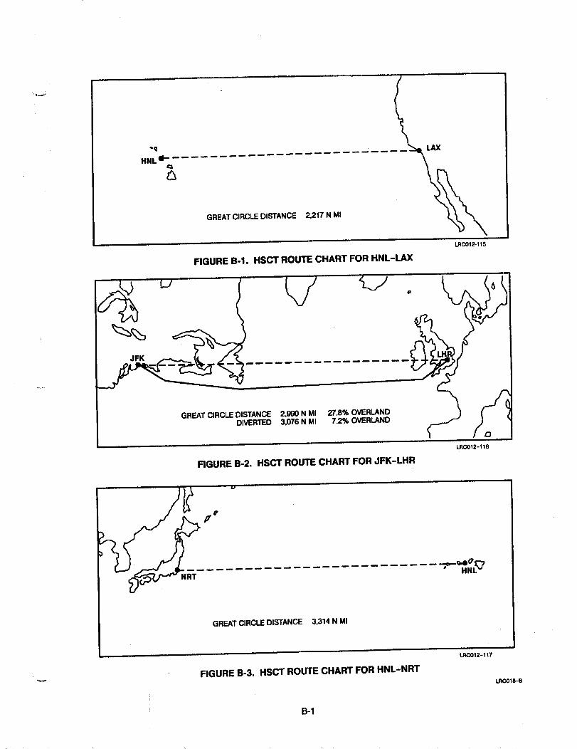
°q

HNL e'-Q

GREAT CIRCLE DISTANCE 2.217 N MI

LRCO12-115

FIGURE B-1. HSCT ROUTE CHART FOR HNL-LAX

GREAT CIRCLE DISTANCE 2.990 N MI 27.8% OVERLANDDIVERTED 3.076 N MI 7.2% OVERLAND

FIGURE B-2. HSCT ROUTE CHART FOR JFK-LHR

LRCO12-116

.... •.-,.r,.- 9,eO _'7• HNL _


FIGURE B-3. HSCT ROUTE CHART FOR HNL-NRT

I.wC0i2-117

LRCO18-B

B-1

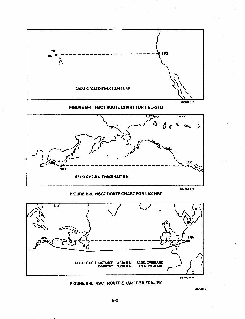
"9_ - SFO

HNL II-- .........

GREAT CIRCLE DISTANCE 2,080 N MI

LRC012.118

FIGURE B-4. HSCT ROUTE CHART FOR HNL-SFO


LRCO12-11g

FIGURE B-5. HSCT ROUTE CHART FOR LAX-NRT

sm

GREAT CIRCLE DISTANCEDIVERTED

3.340 N MI

3,420 N MI

,lm.m m

32.0% OVERLAND )

7.3% OVERLAND _,,"" /_ ]

FIGURE B-6. HSCT ROUTE CHART FOR FRA-JFK

I.RCO12-120

t.RCO18-B

B-2

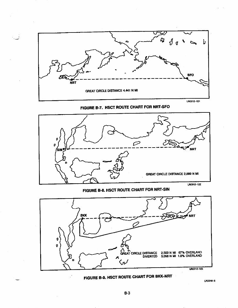
GREAT CIRCLE DISTANCE 4.441 /

/

FIGURE B-7. HSCT ROUTE CHART FOR NRT-SFO

LRC012-121

LRC012-122

FIGURE B-8. HSffT ROUTE CHART FOR NRT-SlN

0

0

GREAT CIRCLE DISTANCE 2,503 N MI 67% OVERLAND

90 , _ ,/_._ DIVERTED 3.056N MI 1.0% OVERLAND,1_ LRC012-123

FIGURE B-9. HSCT ROUTE CHART FOR BKK-NRTLR(_lS-B

B-3

GREAT CIRCLE DISTANCE 3,148 N MI 24.2% OVERLANDDIVERTED 3,194 N MI 4.8% OVERLAND

LRC012-124

FIGURE B-10. HSCT ROUTE CHART FOR CDG-JFK

Q

GREAT CIRCLE DISTANCE 3,705 N MI 28.1% OVERLANDDIVERTED 3,766 N MI 5.8% OVERLAND

_12-125

FIGURE B-11. HSCT ROUTE CHART FOR FCO-JFK

GREAT CIRCLE DISTANCE 3,460 N MI 30.6% OVERLAND

DIVERTED 3,488 N MI 15.8% OVER

FIGURE B-12. HSCT ROUTE CHART FOR JFK-MXP

LRC012-126

LRCO18-B

B-4

FIGURE B-13. HSCT ROUTE CHART FOR GIG-MIA

GREAT CIRCLE DISTANCE 5,845 N MIDIVERTED 6,072 N MI

K

LRCO12-128

FIGURE B-14. HSCT ROUTE CHART FOR JFK-NRT

GREAT CIRCLE DISTANCE 3.176 N MIDIVERTED 3,338 N MI

LRCO12-12g

FIGURE B-15. HSCT ROUTE CHART FOR BRU-JFKLRCOtS-B

B-5

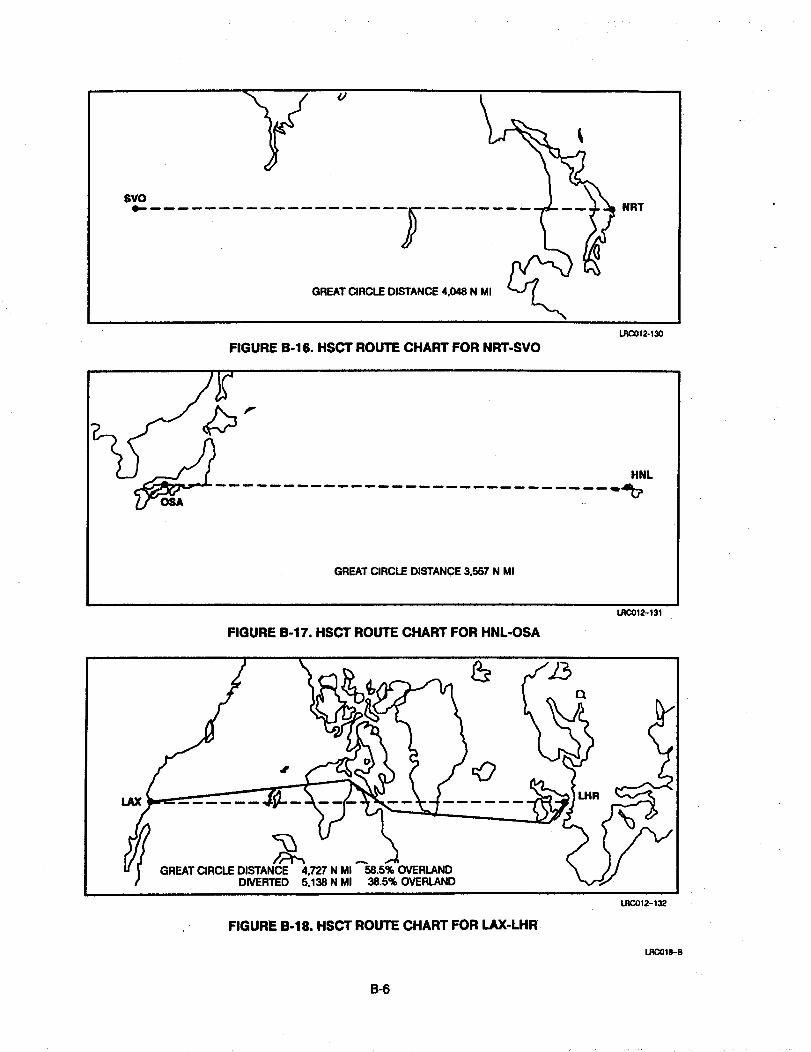
YSVO

tJ


NRT

FIGURE B-16. HSCT ROUTE CHART FOR NRT-SVO

p-

LRCO12-130

HNL

--,,be


FIGURE B-17. HSCT ROUTE CHART FOR HNL-OSA

LRC012-131

FIGURE B-18. HSCT ROUTE CHART FOR LAX-LHR

LRC012-132

LROO|B-B

B-6

FIGURE B-19. HSCl" ROUTE CHART FOR JFK-MAD

i._s_bi 2-133

EWR

GREATCIRCLEDISTANCEDIVERTED

FIGURE B-20. HSCT ROUTE CHART FOR EWR-ORY

l.IT_i 2-134

LLRCO18-B

B-7

T

APPENDIX CGROUND TRACK PROFILE DISPLAY..

250 CITY-PAIRS

LRC018-82

Primary Sort: Overland % HSCT Traffic Network: Top 250 Airport-Pairs By Seats

AIRPORT IATA

# CODES CODE

1HNL-LAX* 12

2 HNL-NRT* 10

3 HNL-SFO* 12

4 LAX-NRT* 10

5 NRT-SFO* 10

6 NRT-S]N" 18

7 SIN-SYD" 18

8 SIN-TPE* 18

9 HNL-SEL* 10

10 AKL-HNL" 11

11HNL-SYD* 11

12 LAX-SEL* 10

13 BKK-SYD* 18

14 HKG-SFO* 10

15 LAX-SYD* 11

16 GIG-JFK* 1

17 LAX-OGG 12

18 PER-SYD* 18

19 BGI-JFK* 2

20 CCS-JFK* 1

210SA-SIN* 18

22 OGG-SFO 12

23 BOM-SIN* 18

24 HNL-MNL" 10

25 JFK-LIS* 3

26 AKL-LAX* 11

27 HKG-SEA* 10

28 GUH-HNL* 10

29 BOS-SNN* 3

30 SEA-SEL 10

31HNL-NAN* 11

32 CGK-NRT 18

33 KUL-MEL 18

34 SFO-TPE" 10

35 AKL-SIN* 18

36 MEL-NAN" 18

37 HKG-SYD 18

38 AMS-AUA" 4

39 AMS-IAH* 3

40 CNS-NRT" 18

41AKL-NRT" 18

42 KUL-NRT* 18

43 HNL-SAN 12

44 FCO-GIG* 5

45 HNL-SJC 12

46 HNL-NGO 10

47 BOS-GLA* 3

48 AMS-BOS* 3

49 HND-HNL 10

50 LAX-PPT* 11

52 BNE-NRT* 18

S] PDX-SEL 10

53 NRT-PDX 10

54 DPS-MEL* 18

55 JFK-KEF* 3

RT

TYP

1

1

1

1

1

1

1

1

1

1

1

1

1

1

1

1

1

1

1

DIST GC Range Overland Diverted Overlan

(SM) (N.Mt.) Oist % Range Dtst %

2551 2217 0 O.O 2217 0 0.0

3813 3314 0 0.0 3314 0 0.0

2394 2080 0 0.0 2080 0 0.0

5440 4727 0 0.0 4727 0 0.0

5112 4441 0 0.0 4441 0 0.0

3324 2889 0 0.0 2889 0 0.0

3908 3360 1892 56.3 5364 0 0.0

2012 1748 0 0.0 1748 0 0.0

4538 3944 181 4.6 4592 0 0.0

4403 3826 0 0.0 3826 0 0.0

5074 4409 66 1.5 4416 0 0.0

5956 5175 0 0.0 5175 0 0.0

4684 4070 2389 58.7 5649 0 0.0

6898 5994 851 14.2 6181 0 0.0 0.00

7490 6508 O 0.0 6508 0 0.0 0.00

4800 4171 1852 44.4 4796 0 0.0 0.00

2481 2156 0 0.0 2156 0 0.0 0.00

2035 1768 1360 76.9 2302 0 0.0 0.00

2091 1816 0 0.0 1816 0 0:0 0.00

1 2115 1837 0 0.0 1837 0 0.0 O.O0

1 3069 2667 0 0.0 2667 0 0.0 0.00

1 2335 2029 0 0.0 2029 0 0.0 0.00

I 2435 2115 632 29.9 3601 0 0.0 0.00

1 5290 4597 0 0.0 4597 0 0.0 0.00

] 3357 2917 0 0.0 2917 0 0.0 0.00

I 6512 5665 0 0.0 5685 0 0.0 0.00

I 6474 5588 1743 31.2 5907 0 0.0 0.00

I 3797 3300 0 0.0 3300 0 0.0 0.00

1 2885 2507 521 20.8 2548 0 0.0 O.OO

1 5180 4501 900 20.0 4566 0 0.0 0.00

I 3171 2755 0 0.0 2755 0 0.0 0,00

l 3623 3148 466 14.8 3245 0 0.0 0.00

I 3946 3429 2500 72.9 4782 0 0.0 0.00

1 6439 5596 716 12.8 5633 0 0.0 O.O0

1 5222 4556 ]904 41.8 4867 O 0.0 O.O0

I 2401 2086 309 14.8 2255 0 0.0 0.00

I 4581 3983 2410 60.5 4497 0 0.0 O.O0

I 4893 4252 272 6.4 4278 0 0.0 O.O0

I 4998 4343 2662 61.3 5055 0 0.0 0.00

1 3653 3174 225 1.l 3435 0 0.0 O.O0

I 5490 4771 0 0.0 4771 0 0.0 0.00

1 3337 2900 0 0.0 2900 0 0.0 0.00

I 2609 2267 0 0.0 2267 0 0.0 0.00

I 5694 4984 2367 47.5 5330 0 0_0 0.00

I 2413 2096 0 0.0 2096 0 0.0 0.00

I 4006 3481 0 0.0 3481 O 0.0 0.00

I 3020 2624 585 22.3 2693 0 0.0 0.00

I 3445 2993 1266 42.3 3141 0 0.0 0.00

I 3845 3983 0 0.0 3983 0 0.0 0.00

I 4105 3569 0 0.0 3569 0 0.0 0.00

1 4472 3886 323 8.3 3940 0 0.0 0.00

I 5252 4564 393 8.6 4606 0 0.0 0.00

I 4810 4180 0 0.0 4180 0 0.0 0.00

I 2726 2262 ]421 62.8 3134 0 0.0 0.00

I 2586 2247 1038 46.2 2451 0 0.0 0.00

0.00

o.oo I ....o.oo I ....o.ooI ....o.ooI ....0.00 I ....

o.oo I ....0.00 I ....

0.00 ....

0.00 ..

Ground Track Length % 1

C_ I 2 3 4 5 6 7 8 9 0

x o o o o o o o o o o oo.ool....I....I....I....I....I....I....I....I....I....Io.ooi....I....I....I....I....I....I....I....I....I....Io.ool .... I .... I .... I .... I .... I .... I .... I.... I .... I .... I

I .... I .... I .... I .... t.... I.... I .... I... I .... t .... I.... I .... I .... I.... i.... I .... I... I .... i .... I.... I .... 1.... ).... I.... i .... I... I .... I .... I.... I .... I .... I .... I .... I .... I... I .... I .... I.... I .... t .... I .... t .... I .... I... I .... I .... I• ..t .... I .... ( .... $.... I .... I... i .... ) ....• ..I .... i .... I .... I .... I .... I .... I .... I ....• ..I .... I .... I ....• ..I .... I .... I ....• ..I .... I .... I ....• ..1.:..I .... I ....

....... I .... I .... I....

........ I .... i .... I....

........ I .... I .... I ....

.... I .... I .... I ........

.... i ....... I .......

.... I...... I...

.... i...... I....... I ...... t....... I ...... I....... I ...... I....... i .... i...

.... i ....

.... I';, . .

.... I .... I .... I .... I ....

.... I .... I .... I .... I ....

.... t .... I .... I .... i ....

.... I .... i .... I .... i ....

.... I.... t .... I .... I ....

.... I .... I .... I .... I ........ I .... i .... I .... I ........ t .... I .... I .... I ........ I .... I .... I .... I .... I.... i .... i .... I .... I .... t.... I .... I .... ¢.... I .... (.... I .... I .... I .... t .... I

..... I .... I .... I .... I .... Ii........ I ........ t.... (

.... i ........ t .... I

.... t ........ I ........ I ...... )-...... I ........ I....... ) ........ I....... I ........ I....... i ........ I...

..... I ........ I...

..... i ....

..... I ....

..... i ....

..... i ....

..... I ....

..... i ....

I .... I ....

I...

E...

I.,.

I...

I.,.

I,.,

I...

I,..

.... I ........ I ....

I .... ;... I .... I .... I ....I.... I... I .... t .... t ....

.... i ....

.... i ....

.... i ....

.... i ....

.... i ....

.... i ....

.... i ....

.... i ....

.... I ....

.... I .... I... I .... I... I .... I..

.... I .... I... I .... I... I....1..

.... I .... I .... I .... Io.. I .... I..

.... t .... I .... i .... (... I .... I..

.... I .... I .... I .... I .... i.... I..

.... i ....

.... I....

.... i ....

.... j ....

.... i ....

.... i ....

.... i ....

.... i ....

• .. I .... I .... I ....I .... I... I .... I... I .... I... I .... I .... I ....I .... i... i .... i... I .... I.. I...t .......I .... i... I .... t... I .... I.. t...i .......I .... I... I .... I... I .... I.. I...t .......I .... i... t .... [... I .... I.. I...I .......

I...I .......I...I .......t .... I ....... )I .... I ....... Ii .... I ....... I

• ( .... i ........ I.... I .... I .... I .... t .... t .... I .... i .... I ........ I.... I .... I .... I .... i .... I .... I .... I .... ( ........ (

I .... I .... I .... I .... I .... I .... I .... I .... I ........ II .... I .... I .... I .... t .... I .... I .... I...,I ......... Ii .... t .... I .... I .... I .... I .... I .... t .... I .... I .... II .... ( .... I .... I .... I .... I .... t .... I .... t .... I .... II .... I .... I .... I .... I .... t .... I .... I .... i .... i .... II .... t .... I .... I .... ( .... i .... I.... i .... I .... I .... 1

Secondary Sort: Seats Configuration: Mach 3.2-Subsonic Overland, 6Hr Curfew. 2hr Turnaround.

C-I

Primary Sort: Over|and %HSCI Traffic Network: lop 250 Airport-Pairs By Seats

AIRPORT ]ATA RT OIST GC Range Overland Diverted Overlan Cum

# CODES CODE TYP (SM) (N.MI.) Olst % Range Oist %

56 NRT-SYD* 18 1 4863 4226 ]040 24.6 4388 22 0.5

57 BKK-NRT* 18 1 2881 2503 1695 67.7 3056 31 1.0

58 AMS-JFK* 3 1 3632 3156 814 25.8 3353 34 I.O

59 JFK-TLV* 3 1 5663 4921 2746 55.8 5178 52 1:0

60 JFK-SNN* 3 I 3072 2669 544 20.4 2716 27 1.0

61LAX-TPE" 10 ] 6770 5883 682 11.6 5898 59 1.0

62 LHR-M]A* 4 ! 4414 3836 36] 9.4 3842 85 2.2

63 JFK-MAN* 3 I 3330 2894 12]0 4].8 3030 70 2.3

64 BKK-SEL* 18 I 2294 ]994 ]603 80.4 2816 68 2.4

65 CMB-DXB* 19 ] 2043 1776 455 25.6 1897 46 2.4

66 BOS-LHR* 3 ] 3254 2827 591 20.9 2956 74 2.5

67 NRT-SEA* 10 I 4757 4133 174 4.2 4144 ]08 2.6

68 DXB-KUL* 19 I 3434 2984 534 17.9 3340 87 2.6

69 GIG-MIA* 1 2 4172 3625 2708 74.7 4149 116 2.8

70 HNL-SEA* 12 I 2675 2325 72 3.1 2325 72 3.1

71BRU-JFK* 3 I 3655 3176 794 25.0 3338 !07 3.2

72 AUH-SIN 19 ] 3672 3190 935 29.3 3486 112 3.2

73 EWR-LHR* 3 I 3454 3002 1324 44.1 3070 98 3.2

74 BOS-LGW* 3 I 3272 2843 847 29.8 2889 95 3.3

75 BO5-BRU* 3 1 3468 30]3 1338 44.4 3097 III 3.6

76 HKG-YVR* 10 I 6368 5534 2308 41.7 5832 216 3.7

77 MIA-SCL* 1 2 4146 3603 1802 50.0 3945 150 3.8

78 ANC-SFO 12 1 2014 1750 67 3.8 ]750 67 3.8

79 ATH-JFK* 3 2 4919 4274 ]607 37.6 4889 220 4.5

80 CDG-JFK* 3 ] 3623 3]48 762 24.2 3194 I47 4.6

81EWR-LGW* 3 1 3472 3018 803 26.6 3183 146 4.6

82 AMS-ATL" 3 I 4388 3812 1395 36.6 4157 ]91 4.6

83 CDG-MIA* 4 ] 4577 3977 183 4.6 3977 183 4.6

84 EZE-MAD* 5 ] 6257 5437 2409 44.3 5712 263 4.6

85 GUA-LAX* 2 ] 2193 1905 1905 100.0 211] 99 4.7

86 EWR-ORY* 3 ] 3638 3161 699 22.1 330] ]58 4.8

87 GIG-HAD* 5 I 5058 4396 725 16.5 4444 213 4.8

88 LGW-MIA* 4 I 4429 3849 362 9.4 3859 185 4.8

89 JFK-MEX* 2 2 2090 1816 1115 61.4 2022 99 4.9

90 CPH-JFK* 3 ! 3843 3340 792 23.7 3451 169 49

9L NRT-YVR* 10 1 4663 4052 288 7.] 4069 208 5.1

92 AUH-CGK 19 1 4101 3563 1290 36.2 3689 192 5.2

93 IAH-LGW* 3 1 4840 4210 2404 57.1 4826 256 5.3

94 GIG-LHR* 5 1 5746 4893 1316 26.9 5062 268 5.3

95 JFK-ORY* 3 1 3623 3148 711 22.6 3181 ]72 5.4

96 BOS-CDG* 3 I 3436 2967 629 21.2 3022 ]69 5.6

97 FCO-JFK* 3 2 4264 3705 1041 28.1 3766 218 5.8

98 FRA-GIG* 5 ] 5942 5164 1513 29.3 5370 3!] 5.8

99 MAD-MIA* 4 ] 4413 3834 238 6.2 3834 238 6.2

IO0 LHR-PHL* 3 1 3533 3070 1461 47.6 3145 198 6.3

IO] BCN-JFK* 3 I 3820 3319 461 13.9 3458 218 6.3

102 AMS-PBM* 4 1 4674 4061 256 6.3 4061 256 6.3

103 OUS-JFK 3 ! 3736 3247 1555 47.9 3364 212 6.3

104 CCS-MAD* 4 I 4349 3779 242 6.4 3779 242 6.4

105 FRA-MIA* 4 ] 4820 4188 725 17.3 42]0 274 6.5

106 BKK-OSA* ]8 1 2601 2264 1598 70.6 2789 181 6.5

107 HAV-YQX 2 I 2345 2037 139 6.8 2037 139 6.8

I08 ATL-LGW* 3 1 42]6 3664 ]718 46.9 3826 264 6.9

109 L]M-MIA* 1 2 2620 2277 ]025 45.0 2647 I83 6.9

110 MAD-MEX* 4 I 5631 4893 499 10.2 4970 353 7.!

Secondary Sort: Seats

6round Track Length % I

1 2 3 4 5 6 7 8 9 0

o o o o o o o o o o o0.041 .... I .... I .... I .... I .... I.... I .... I .... I .... I .... I0.10". .... I .... I .... I .... I .... I .... I .... I .... I....I .... *0.151 .... I .... I .... I .... I .... I .... I .... I .... I .... I .... *0.231 .... I .... I .... I.... I .... I .... I .... I .... I.... I .... *0.261 .... I .... I .... I .... I .... I .... I .... I .... I .... I .... *o.32 *....I .... I .... I .... I .... I .... I ........ I .... I .... I0.42 *....I .... I .... I .... I .... I.... I ........ I .... i .... Io.sol .... I .... I .... I .... I .... I .... I ........ I .... I .... *0.56"....I .... I .... I .... I .... I .... I ........ I.:..I .... *0.611 .... I .... I .... I .... I .... I .... I ......... I .... I .... *0.671 .... I .... I .... I....I .... I .... I ........ I .... I...**0.761 .... I .... I .... I .... I .... I .... I .... I .... I .... I .... *0.63"...,I .... I .... I .... I .... I .... I .... I .... I .... I .... *0.921 .... I .... I*...I .... I .... I .... I .... I .... I .... I .... I0.971 .... I.... I .... I .... I .... I .... I .... I .... I .... I...**!.04 *"...I .... I .... I .... I .... I .... I .... I ...I .... I .... I1.!1 **...I .... I .... I .... I....I .... I .... I ...I .... I .... I1.171 .... I .... I .... I .... I .... I .... I .... I ...I .... I...**1.231 .... I .... I .... I .... I .... I .... I .... I ...I .... I...**1.291 .... I .... I .... I .... I .... I .... I .... I ...I .... 1...**1.411 .... I .... I .... I .... I .... I .... I .... I ...1_...I...**1.491 .... I .... I*"..I .... I .... I .... I .... I....I .... I..:.11.52 **...I .... I .... I .... I .... I .... I .... I .... I .... I .... I1.631 .... **...I .... I .... I .... I .... I .... I .... I .... I .... I1.70 ***..I .... I .... I .... I .... I .... I .... I .... I .... I .... I].771 .... I .... I .... I .... I ...... I .... I .... I .... I .... I...**1.851 .... I .... I .... I .... I .... I .... I.... I .... I .... I...*].93 ***..I .... I .... I .... I .... I .... I .... I .... I .... I .... i_2.031 .... I .... I .... I .... I .... I .... I .... I .... I .... I..***2.07 **...I .... J.... I .... J.... J.... I .... I .... I .... I .... I2.121 .... I .... I .... I .... I .... I .... I .... I .... I .... I...**2.201 .... I .... I .... I .... I .... I .... I .... I .... I .... I-.***2.26 ***..I .... I .... I .... I .... I .... I .... I .... I .... I .... I2.291 .... I .... I .... I .... **...1:...I .... I .... I .... I.-*"*2.34 ***..I .... I .... I .... I .... I .... I .... I .... I .... I .... I2.4!1 .... I .... I .... I .... I .... I .... I .... I .... I .... I..**"2.47"*...I .... i .... I .... I .... I .... I .... I .... I .... I .... *2.541 .... I .... I .... I .... I .... I .... I .... I .... I .... I.-***2.621 .... I .... I .... I .... I .... I .... I .... i .... I .... I.*'**2,661 .... I .... I .... I .... I .... I .... I .... I .... I .... I.-***2.7!1 .... I .... I .... I .... I .... I .... I .... I .... I .... I..***2.771 .... I***.1 .... I .... I .... I .... I .... 1.... I .... I .... I2.65 ***..i .... I .... I .... I .... I .... I .... I .... I .... I .... I2.9J.***..I .... I .... I .... I .... I .... I .... I .... i .... I .... I2.96"...I .... I .... I .... I .... I .... I .... I .... I .... I .... *3.02 "*..I .... I .... I .... I .... I .... I .... I .... I .... I .... I3.o8 *'*..I .... i .... I .... I .... I .... I .... I .... I .... I .... I3.13 **'..I .... I .... I .... I .... I .... I .... I .... I .... I .... i3.]81 .... I .... I .... I.:..I .... I .... I .... I .... I .... I-.***3.24 ***..I .... I .... I .... I .... I .... I .... I .... I .... I .... I3.28 **...I .... I .... I .... I .... I .... I .... I .... I.:..I..***3.311 .... I .... I .... I .... I .... I .... I .... I .... I .... I..***3.37"*...I .... I .... I .... I .... I .... I .... I .... I .... I .... *3.41 *....I .... I...***...I .... I .... I .... I .... I .... I .... I3.48 **'..I .... I .... I....I .... I .... I .... I .... I .... I...**

Configuration: Mach 3.2-Subsonic Overland, 6Hr Curfew, 2hr Turnaround.

C-2

Primary Sort: Overland % HSCT Traffic Network: Top 250 Airport-Palrs By Seats

AIRPORT IATA

# CODES CODE TYP (SM)

III FDF-ORY* 4 1 4255

112 JFK-LHR* 3 1 3441

113 JFK-LGW* 3 1 3459

I14 FRA-JFK* 3 I 3844

115 OSA-SFO 10 1 5374

116 HNL-OSA* 10 I 4093

117 AMS-YMX* 3 1 3429

118 DRY-PIP 4 I 4193

119 BOS-FRA* 3 1 3657

120 JFK-MAD* 3 1 3578

121CDG-FDF* 4 1 4266

122 ANC-NRT* 10 1 3426

123 MAD-SDQ* 4 I 4154

124 CDG-PTP* 4 1 4204

125 CDG-IAD* 3 ] 3848

126 FRA-IAD* 3 I 4067

127 ]AD-LHR* 3 1 3665

128 BO5-ZRH* 3 1 3732

I29 BRU-YMX* 3 1 3461

130 ANC-SEL* 10 1 3769

131HNL-LAS* 12 I 2757

]32 ARN-JFK* 3 I 3908

133 HNL-PHX 12 I 2910

I34 ATL-FRA* 3 I 4600

135 CVG-LBW 3 I 3969

136 LHR-YMX" 3 1 3251

137 AMS-YYZ* 3 I 3720

138 CPH-SEA * 3 2 4849

139 CDG-YMX* 3 I 3444

140 6VA-JFK* 3 I 3852

]410FW-SJU* 2 1 2163

142 LHR-NRT* 9 2 5954

143 JFK-WAW" 3 I 4253

144 FRA-YMX* 3 1 3647

14_ PER-SIN* 18 I 2428

146 ATL-MUC 3 I 4786

147 FRA-YYZ*

148 HEL-JFK*

|49 LGW-NRI

]50 AMS-ORD

I5! JFK-MXP*

152 ATH-SIN

153 JFK-MUC*

154 CVG-FRA

155 EZE-MIA*

156 FRA-NRT*

157 CVG-ORY*

158 DTW-NRT

|59 DTW-SEL

160 LGW-MSP

161COG-DTW

162 JFK-ZRH*

163 BOG-JFK

164 BRU-ORD*

165 LGW-YYZ*

RT DIST GC Range Overland Diverted Overlan

(N.Mi.) Dist % Range" Oist %

3697 262 7.1 3697 262 7.1

2990 831 27.8 3076 221 7.2

2996 833 27.8 3082 222 7.2

3340 1069 32.0 3420 250 7.3

3643 270 7.4 3643 270 7.4

3557 263 7.4 3557 263 7.4

2979 1341 45.0 3312 255 7.7

4670 369 7.9 4670 369 7.9

3178 953 30.0 3312 265 8.0

3109 255 8.2 3]09 255 8.2

3707 308 8.3 3707 308 8.3

2977 444 14.9 3031 255 8.4

3609 303 8,4 3609 303 8.4

3653 321 8.8 3653 321 8.8

3344 883 26.4 3376 300 8.9

3534 1428 40.4 3619 362 10.0

3185 1271 39.9 3260 339 10.4

3243 1281 39.5 3290 345 10.5

3007 1320 43.9 3269 350 10.7

3275 874 26.7 3417 372 10.9

2395 266 II.l 2395 266 lI.I

3382 1383 40.9 3536 392 ll.l

2529 281 11.1 2529 281 11.1

3998 1915 47.9 4179 485 11.6

3450 1846 53.5 3653 424 11.6

2825 1212 42.9 3200 384 12.0

3232 1587 49.1 3625 442 12.2

4214 2748 65.2 5074 624 12.3

2993 1116 37.3 3203 400 12:5

3347 1406 42.0 3377 422 12.5

1879 586 31.2 1941 247 ]2.7

5147 3829 74.4 5880 759 12.9

3695 1655 44.8 3828 532 13.9

3169 1534 48.4 3425 493 I4.4

2110 306 14.5 2110 306 14.5

4159 2583 62.1 4376 639 14.6

3 1 3939 3423 1089 31.8 3699 544 14.7

3 1 4103 3566 1562 43.8 3746 566 15.1

9 2 5967 5149 4289 83.3 5448 844 15.5

3 1 4106 3568 1745 48.9 4028 628 15.6

3 1 3983 3460 |059 30.6 3488 551 15.8

9 2 5626 4889 3545 72.5 5232 832 ]5.9

3 I 4028 3501 1390 39.7 3549 568 16.0

3 1 4347 3778 2059 54.5 4194 688 16.4

1 2 4409 3831 2984 77.9 4137 691 16.7

9 2 5814 5053 4073 80.6 5211 917 17.6

3 1 4144 3601 1426 39.6 3700 651 17.6

10 2 6380 5544 3321 59.9 6083 1077 17.7

10 2 6603 5737 4211 73.4 6314 1124 17.8

3 1 4022 3495 1754 50.2 3942 706 17.9

3 1 3948 3431 1791 52.2 3575 651 18.2

3 1 3919 3405 1611 47.3 3441 630 18.3

I I 2481 2156 395 18.3 2156 395 18.3

3 I 4145 3602 1740 48.3 3966 738 18.6

3 I 3564 3097 1505 48.6 3347 653 19.5

Ground Track Length % 1

Cum I 2 3 4 5 6 7 8 9 0

% O 0 0 O 0 O 0 0 O O O

3.541 .... I .... I .... I .... I .... I .... I .... I .... I .... I.****3.56 **...I .... I .... I .... I .... I .... I .... I .... I .... I...**3.63 **...I .... I .... I .... I .... I .... I .... I .... I .... I...**3.68"**..I ........ I .... I .... I .... I.:..I .... I .... I .... *3.73 .... .[ ........ I ........ I .... I .... I .... I .... I .... I

3.781 .... I ........ I ........ I .... I .... I .... I.... I..***3.821 .... I ........ I ........ I .... I .... I.... I .... I.****3.89 .... .I ........ I ........ I .... I .... I .... I .... I .... I3.941 .... I ........ I ........ I .... I .... I .... I..:.1.****3.991 .... ] .... I .... ] ........ I .... I .... I.._.1 .... I.****

4.05 .... .I .... I .... I .... I .... I....I .... I .... I .... I .... I4.09 .... .I .... I .... I .... I .... I .... I .... I .... I .... I .... I4.I5 ..... I .... I .... I .... I .... I .... I .... I .... I .... I .... I4.21 ..... I .... I .... I .... I .... I .... I .... I .... I .... I .... I4.26 **...I .... I .... I .... I .... I .... I .... I .... I .... I..***4.33 *'*..I .... I .... I .... I .... I .... I .... I .... I .... I...*"4.39 **...I .... I .... I .... I .... I .... I .... I .... I .... I..***

4,461 .... I .... I .... I .... I.... I .... I .... I .... I .... *.....4.52"*...I .... I .... I .... I .... I .... I .... I .... I .... I.****4.59 .... .I .... l .... l .... I .... l .... I .... I .... I .... I .... *4.641 .... I .... I .... I .... I .... I .... I .... I .... I .... *.....4.71 ..... I .... I .... I .... I .... I .... I .... I .... I .... I .... I4.761 .... I .... I .... I .... I .... I .... I .... I ........ *......4.85 *'...I .... I .... I .... I .... I .... I .... I .... I .... I. *'*°4.93 ...... ..-.I .... I .... I .... I .... I .... I .... I .... I .... *4.99 ***..I .... I .... I .... I .... I. .... I .... I .... I .... I..***5.071 .... I .... I .... I .... I .... I .... I .... I ........ *......s.ze **...I .... I .... I .... I .... I .... I .... ****-I .... I .... *S.2S***..I .... I .... I .... I .... I .... I .... I .... I .... I ."**"5.32 ....... .-.I .... I .... I .... I .... I .... I .... I .... I .... I5.36 ....... ...I .... I .... I .... I .... I .... I .... I .... I .... I5.48*....I .... I .... I .... I .... I .... I.* .... --.I .... I .... *S.S71.... I .... I .... I .... I .... I .... I .... I .... I.-* .......S.6S.... -I .... I .... I .... I .... I .... I .... I .... I .... I .... I5.71 ....... -..I .... I .... I .... I .... I .... I .... I .... I .... I5.81 ***.-I .... I .... I .... I .... I .... I .... I .... I .... I.....5.90 ***..I .... I .... I .... I .... I .... I .... I .... I .... I.****5.99 ........ --I .... I .... I .... I .... I .... I .... I .... I .... I6.13 *...-I .... I .... I .... I .... I .... I-.-* ..... I .... I .... *6.22 ........ ..I .... I .... I .... I .... I .... I .... I .... I .... I6.311 .... I .... I .... I .... I .... I .... I .... I .... I-.* .......6.441 .... I.* ...... .I...*I .... I .... I .... I .... I .... I .... I6.52 ........ ..I..:.I .... I .... I .... I .... I .... I .... I .... I6.62 ...... ...-I .... I_.:.I .... I .... I .... I .... I .... I--***6.73 ........ ..I .... I .... I .... I .... I .... I..*.I .... I*-..I6.86 *..-.I .... I .... I .... I .... I .... I.* ....... I .... I.... *0.96 ........ ..I .... I .... I .... I .... I .... I .... I .... I-..**7.IZ ..... I .... I..* .... ..I .... I .... I .... I .... I .... I .... I7.27 ..... I .... I-.* .... ..I .... I .... I .... I .... I .... I .... I7,371 .... I .... I .... I .... I .... I .... I .... I .... I..........7.46 ........ ..I .... I .... I .... I .... I .... I .... I .... I..-**7.541 .... I .... I .... I .... I .... I .... I .... I .... I.* ........7.59 .......... I .... I .... I .... I .... I .... I .... I .... I .... I7.69 **...I .... I .... I .... I .... I .... I .... I .... I--* .......7.78 "**-.I .... I .... I .... I .... I .... I .... I .... I.-**** ....

Secondary Sort: SeatsConfiguration: Mach 3.2-Subsonic Overland. 6Hr Curfew, 2hr Turnaround.

C-3

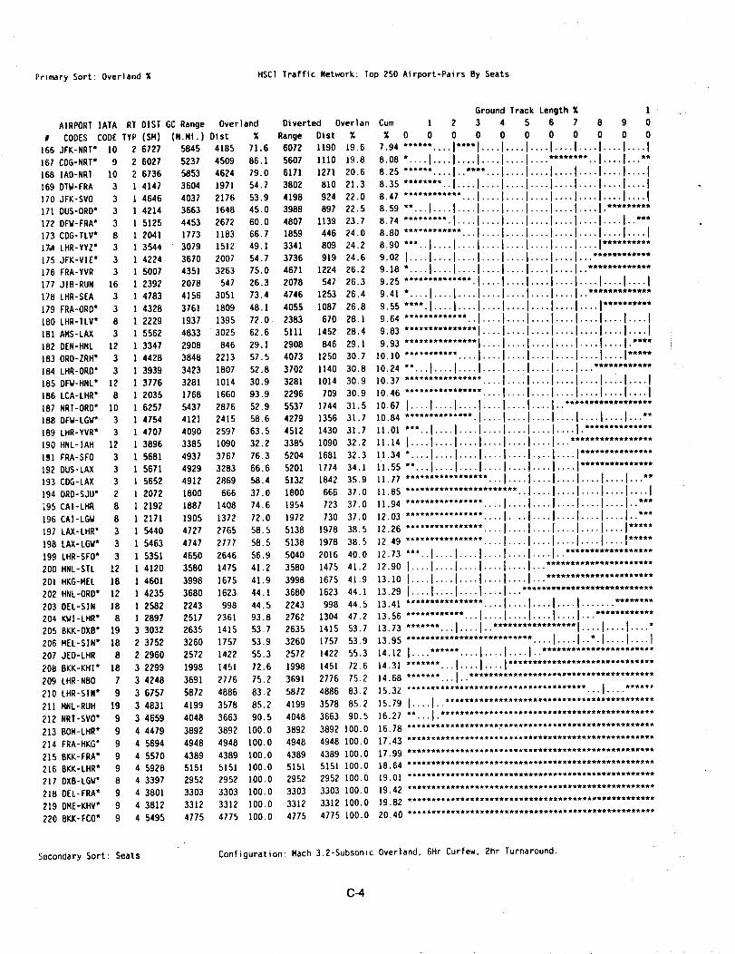
Primary Sort: Overland % HSCT Traffic Network: Top 250 Airport-Pairs By Seats

AIRPORT ]ATA RT DIST GC Range Overland

# CODES CODE TYP (SM) (N.MI.) Oist %

166 JFK-NRT* 10 2 6727 5845 4185 71.6

167 COG-NRT* 9 2 6027 5237 4509 86.1

168 IAD-NRT 10 2 6736 5853 4624 79.0

169 DTW-FRA 3 1 4147 3604 1971 54.7

170 JFK-SVO 3 1 4646 4037 2176 53.9

171DUS-ORD* 3 1 4214 3663 1648 45.0

172 DFW-FRA* 3 l 5125 4453 2672 60.0

173 CDG-TLV* 8 1 2041 1773 1183 66.7

17_ LHR-YYZ * 3 1 3544 3079 1512 49.1

175 JFK-VIE* 3 I 4224 3670 2007 54.7

176 FRA-YVR 3 ] 5007 4351 3263 75.0

177 JIB-RUN 16 I 2392 2078 547 26.3

178 LHR-SEA 3 [ 4783 4156 3051 73.4

179 FRA-ORD* 3 I 4328 3761 1809 48.1

180 LHR-TLV* 8 l 2229 1937 1395 72.0

181AMS-LAX 3 1 5562 4833 3025 62.6

182 DEN-HNL 12 I 3347 2908 846 29.]

183 ORD-ZRH* 3 I 4428 3848 2213 57.5

184 LHR-ORD* 3 ] 3939 3423 ]807 52.8

185 DFW-HNL* 12 1 3776 3281 1014 30.9

186 LCA-LHR* 8 I 2035 1768 1660 93.9

187 NRT-ORD* 10 ] 6257 5437 2876 52.9

188 DFW-LGW* 3 ] 4754 4121 24]5 58.6

189 LHR-YVR* 3 I 4707 4090 2597 63.5

190 HNL-IAH 12 I 3896 3385 1090 32.2

191 FRA-SFO 3 I 5681 4937 3767 76.3

192 DUS-LAX 3 [ 5671 4929 3283 66.6

193 CDG-LAX 3 ] 5652 4912 2869 58.4

194 ORD-SJU* 2 ] 2072 1800 666 37.0

195 CAI-LHR 8 1 2192 1887 1408 74.6

196 CAI-LGW 8 1 2171 1905 1372 72.0

197 LAX-LHR" 3 I 5440 4727 2765 58.5

198 LAX-LGW* 3 I 5463 4747 2777 58.5

199 LHR-SFO* 3 1 5351 4650 2646 56.9

200 HNL-STL 12 1 4120 3580 1475 41.2

20] HKG-MEL 18 ] 4601 3998 1675 41.9

202 HNL-ORD* 12 I 4235 3680 1623 44.1

203 DEL-SIN 18 I 2582 2243 998 44.5

204 KWI-LHR* 8 1 2897 2517 2361 93.8

205 BKK-DXB* 19 3 3032 2635 1415 53.7

206 MEL-SIN* 18 2 3752 3260 1757 53,9

207 JED-LHR 8 2 2960 2572 1422 55.3

208 8KK-KHI* 18 3 2299 1998 1451 72.6

209 LHR-NBO 7 3 4248 3691 2716 75.2

210 LHR-SIN* 9 3 6757 5872 4886 83.2

21] MNL-RUH 19 3 4831 4199 3578 85.2

212 NRT-SVO* 9 3 4659 4048 3663 90.5

213 BOM-LHR* 9 4 4479 3892 3892 I00.0

214 FRA-HKG* 9 4 5694 4948 4948 100.0

215 BKK-FRA" 9 4 5570 4389 4389 100.0

216 BKK-LHR* 9 4 5928 5151 5151 100.0

217 DXB-LGW* 8 4 3397 2952 2952 IO0.O

218 DEL-FRA" 9 4 3801 3303 3303 lO0.O

219 DME-KHV* 9 4 3812 3312 3312 100.0

220 BKK-FCO* 9 4 5495 4775 4775 I00.0

Diverted Overlan

Range Dlst %

6072 1190 19.6

5607 1110 19.8

6171 1271 20.6

3802 810 21.3

4198 924 22,0

3988 897 22.5

4807 1139 23.7

1859 446 24.0

3341 809 24.2

3736 919 24.6

4671 1224 26.2

2078 547 26.3

4746 1253 26.4

4055 1087 26.8

2383 670 28.1

5111 1452 28.4

2908 846 29.1

4073 1250 30.7

3702 1140 30.8

3281 1014 30.9

2296 709 30.9

5537 1744 31.5

4279 1356 31.7

4512 1430 31.7

3385 1090 32.2

5204 1681 32.3

5201 1774 34.1

5132 1842 35.9

1800 666 37.0

1954 723 37.0

1972 730 37.0

5138 t978 38.5

5138 1978 38.5

5040 2016 40.0

3580 1475 41.2

3998 1675 41.9

3680 1623 44.1

2243 998 44.5

2762 1304 47.2

2635 1415 53.7

3260 1757 53.9

2572 ]422 55.3

1998 1451 72.6

3691 2776 75.2

5872 4886 83.2

4199 3578 85.2

4048 3663 90.5

3892 3892 100.0

4948 4948 100.0

4389 4389 100.0

5151 5151 100.0

2952 2952 100.0

3303 3303 100.0

3312 3312 100.0

4775 4775 100.0

Ground Track Length %

Cum 1 2 3 4

% 0 0 0 0 0

7.94 ...... ....1"***1 .... I8.o8*....I .... I .... I .... I825 ...... ....I..****...I8.3s........ ..I .... I .... I8.47 ............ -..I .... I

8.59 **...I .... I .... I .... I8.74......... .I .... I .... I8.80............ ...I....I8.90***..I .... I .... I .... I9.02 I .... I .... I .... I .... I

5 6 7

0 0 0

•..I .... I .... I..•.. ] .... t1_***_t*

•..I ........ I.....I ........ I.....J.., ..... J..•..I ........ I..I ........ I..•..I ........ I.....I ........ I..

1

8 9 0

0 0 0

.I ...I .... I•I ...I...**•I ...I .... I•I ...I .... I.I ...I .... I

.I .._.1..***

.I ...I .... I

.IWW*W**wwww

9.18*....I .... I .... I .... I...I ....9.25 .............. .I .... I...I ....

9.41*....I....I....I....I....I....9.5s .... .I .... I .... I .... I .... I.9.64 ............. ..I .... I .... I.9.83............... I....I....I.9.93 ............... I .... I .... I.

10.10........... ....I .... I .... I.10.24**...I .... I .... I .... I .... I.I0.37 ................ ...-I .... I.

10.46 ................ .---I .... I-

.... I .... I .... I .... I

**1 .... I .... I*" .... **'*

..I .... I .... I .... I .... I

..I .... I .... I .... I .... I

..I .... I .... I .... I.....

..I .... I..: ...........

..I....I .... I .... I .... I

..I .... I .... I .... I .... I10.671.... I .... I .... I .... I .... I .... I..* .................]0.84 .............. .I .... I .... I .... I .... I .... I .... I...**11.ol ***..I .... I .... I .... I .... I .... I .... I.* .............11.141....I....I....I....I....I....I11.34*....I....I....I....I....I....I11.s5**...I .... I .... I .... I .... I .... I11.77................. ...I....I....I11.85....................... ..I....I11.94................ ....I .... I .... I12.o3....................I....I....I

•..I....I....I...-•..I....I....I....I•..I....I....I..***•..I....I....I..*-

12.26................ ....I....I....I....I....I....I.....12.49................ ..--I .... I .... I .... I .... I .... I.....12.73***..I .... I .... I .... I .... I .... I..* .................12.901.... I .... I .... I .... I .... I.-.* .....................13.1oI .... I .... I .... I .... I .... I...* ................ *....13.29I .... I .... I .... I .... I...* ..........................13.41................ ....I .... I .... I .... I ....... * .......13.56............ ...I....I....I....I....I...*...........13.73....... .-.I .... I..* ................ I .... I .... I .... *13.95.......................... ....I .... I..*.1 .... I .... I14.12 I .... * ..... :...1 .... I .... I..* ......................14.31....... ...I .... I .... I..............................]4.68 ***************************************************

15.32 ..................................... -..J .... * .....

15.79 J .... I--* ..........................................

16.27 ***************************************************

16.78 ***************************************************

17,43 ***************************************************

17.99 ***************************************************

18.64 ***************************************************

19.01 ***************************************************

19.42 ***************************************************

19.82 ***************************************************

20,40 ***************************************************

Secondary Sort: Seats Configuration Mach 3.2-Subsonlc Overland. 6Hr Curfew. 2hr Turnaround.

C_4

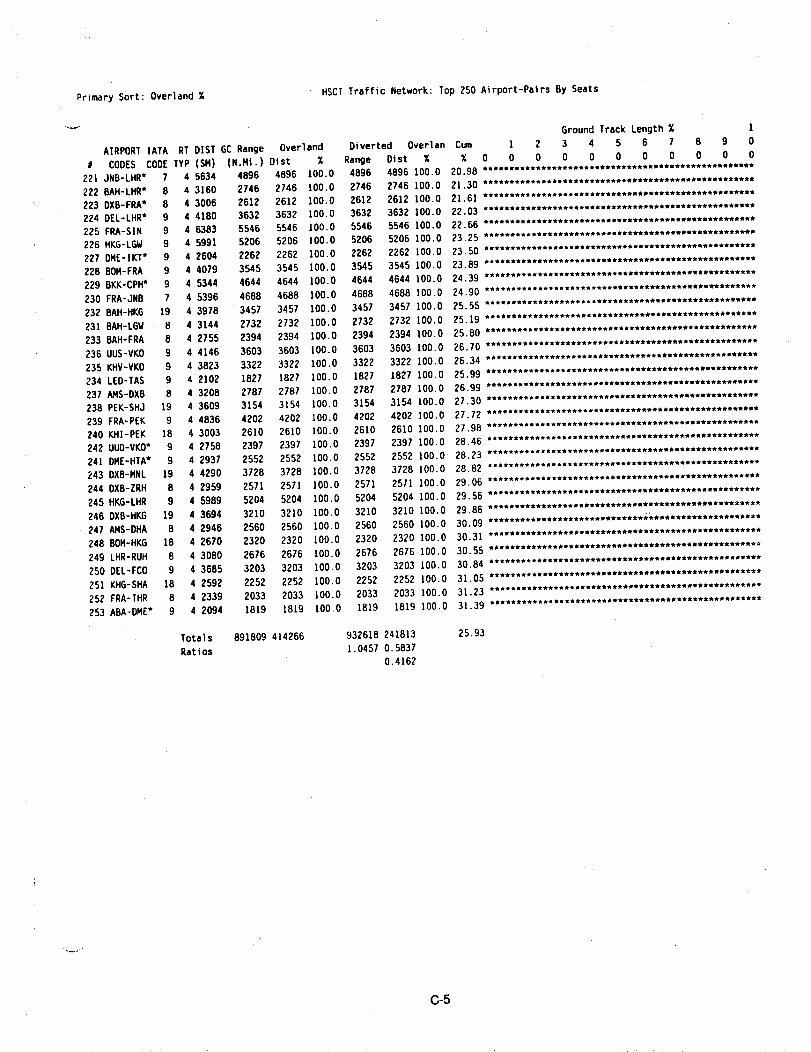
HSCT Traffic Network: Top 250 Airport-Pairs By SeatsPrimary Sort: Overland %

AIRPORT ]ATA RT DIST GC Range Overland Diverted

# CODES CODE TYP (SN) (N.Mi.) Dist % Range

221JNB-LHR* 7 4 5634 4896 4896 100.0 4896

222 BAH-LHR* 8 4 3160 2746 2746 100.0 2746 2746 100.0

223 DXB-FRA* 8 4 3006 2612 2612 ]00.0 2612 2612 100.0

224 DEL-LHR* 9 4 4180 3632 3632 100.0 3632 3632 ]00.0

225 FRA-SIN 9 4 6383 5546 5546 100.0 5546 5546 100.0

226 HKG-LGW 9 4 5991 5206 5206 100.0 5206 5206 100.0

227 OME-IKT* 9 4 2604 2262 2262 100.0 2262 2262 100.0

228 BOM-FRA 9 4 4079 3545 3545 100.0 3545 3545 100.0

229 BKK-CPH* 9 4 5344 4644 4644 100.0 4644 4644 100.0

230 FRA-JNB 7 4 5396 4688 4688 100.0 4688 4688 100.0

232 BAH-HKG 19 4 3978 3457 3457 100.0 3457 3457 100.0

231 8AH-LBW 8 4 3144 2732 2732 100.0 2732 2732 IO0.O

233 BAH-FRA 8 4 2755 2394 2394 100.0 2394 2394 100.0

236 UUS-VKO 9 4 4146 3603 3603 100.0 3603 3603 100.0

235 KHV-VKO 9 4 3823 3322 3322 100.0 3322 3322 100.0

234 LED-TAS 9 4 2102 1827 1827 100.0 1827 1827 100.0

237 AMS-OXB 8 4 3208 2787 2787 100.0 2787 2787 100.0

238 PEK-SHJ 19 4 3609 3154 3154 100.0 3154 3154 100.0

239 FRA-PEK 9 4 4836 4202 4202 100.0 4202 4202 ]00.0

240 KHI-PEK 18 4 3003 2610 2610 100.0 2610 2610 100.0

242 UUD-VKO* 9 4 2758 2397 2397 100.0 2397 2397 100.0

241DME-HTA* 9 4 2937 2552 2552 100.0 2552 2552 100.0

243 DXB-MNL 19 4 4290 3728 3728 100.0 3728 3728 100.0

244 OXB-ZRH 8 4 2959 2571 2571 100.0 2571 2571 100.0

245 HKG-LHR 9 4 5989 5204 5204 100.0 5204 5204 100.0

246 DXB-HKG ]9 4 3694 3210 3210 100.0 3210 3210 100.0

247 AHS-DHA 8 4 2946 2560 2560 100.0 2560 2560 100.0

248 BOM-HKG 18 4 2670 2320 2320 100.0 2320 2320 100.0

249 LHR-RUH 8 4 3080 2676 2676 100.0 2676 2676 100.0

250 DEL-FCO 9 4 3685 3203 3203 100.0 3203 3203 100.0

251KHG-SHA 18 4 2592 2252 2252 100.0 2252 2252 100.0

252 FRA-THR 8 4 2339 2033 2033 100.0 2033 2033 100.0

253 ABA-DME* g 4 2094 1819 1819 100.0 1819 1819 100.0

Totals 891809 414266 932618 241813

Ratios 1.0457 0.58370.4162

Ground Track Length % I

Overlan Cum I 2 3 4 5 6 7 8 9 0

Dist % % 0 0 0 0 0 0 0 0 0 0 0

4896 100.0 20.98 ***************************************************

25.93

C-5

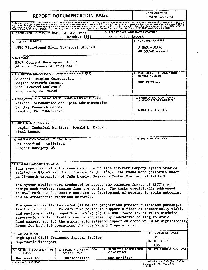
Form Apl_roved

REPORT DOCUMENTATION PAGE OMBNo.0704-0188

Public reporting burden for this co iection of informat on s estimated to average 1 hour per response, including the time for rewewing instructions, searching existing data sources,

gather ng and ma nta n ng the data needed, and completing and reviewing the collection of information. Send comments rec_arding this burden estimate or any other aspect of thiscollect on of information including suggestions for reducing this burden, to Washington Headquarters Services, Directorate tor Information Operations and Reports, 1215 Jefferson

Davis Highway, Suite 1204. Arlington, VA 22202.4302. and to the Off ce of Management and Budget, Paperwork Reduction Prc iect (0704-0188), Washington, DC 20503.

1. AGENCY USE ONLY (Leave b/ank) 2. REPORT DATE

October 1992

4. TITLE AND SUBTITLE

1990 High-Speed Civil Transport Studies

6. AUTHOR(S)

HSCT Concept Development Group

Advanced Commercial Programs

7. PERFORMING ORGANIZATION NAME(S) AND ADDRESS(ES)

McDonnell Douglas Corporation

Douglas Aircraft Company

3855 Lake_cood Boulevard

Long Beach, CA 90846

9. SPONSORING/MONiTORING AGENCY NAME(S) AND ADDRESS(ES)

National Aeronautics and Space Administration

Langley Research Center

Hampton, VA 23665-5225

11. SUPPLEMENTARY NOTES

3. REPORT TYPE AND DATES COVERED

Contractor ReportS. FUNDING NUMBERS

C NASl-18378

WU 537-01.22-01

8. PERFORMING ORGANIZATION

REPORT NUMBER

HDC K0395-2

10. SPONSORING / MONITORINGAGENCY REPORT NUMBER

NASA CR-189618

Langley TechnicalMonitor: Donald L. Maiden

Final Report

12a. DISTRIBUTION / AVAILABILITY STATEMENT

Unclassified - Unlimited

Subject Category 05

12b. DISTRIBUTION CODE

13. ABSTRACT(Maximum200wor_)

This report contains the results of the Douglas Aircraft Company system studies

related to High-Speed Civil Transports (HSCT's). The tasks were performed under

an 18-month extension of NASA Langley Research Center Contract NASI-18378.

The system studies were conducted to assess the emission impact of HSCT's at

design Hach numbers ranging from 1.6 to 3.2. The tasks specifically addressed

an HSCT market and economic assessment, development of supersonic routenetworks,

and an atmospheric emissions scenario.

The general results indicated (I) market projections predict sufficient passenger

traffic for the 2000 to 2025 time period to support a fleet of economically viable

and environmentally compatible HSCT's; (2) the HSCTroute structure to minimize

supersonic overland traffic can be increased by innovative routing to avoid

land masses; and (3) the atmospheric emission impact on ozone would be significantl]

lower for Mach 1.6 operations than for Mach 3.2 operations.

J4. SUBJECTTERMS

High, Speed Civil Transport Systems Studies

Supersonic Transport

17. SECURITY CLASSIFICATIONOF REPORT

Unclassified

NSN 7540-01-280-5500

18. SECURITY CLASSIFICATIONOF THIS PAGE

Unclassified

19. SECURITY CLASSIFICATIONOF ABSTRACT

15. NUMBER OF PAGES

8116. PRICE CODE

A0520. LIMITATION OF ABSTRACT

UnclassifiedStandard Form 298 (Rev. 2-89i "'

Prescribed by ANSI Std Z39-_8298-102

NASA Contractor Report 189618 qS · assessment, and Alan K. Mortlock, technical assessment. Other Douglas staff that made essential contributions to the HSCT team contract work included:

Documents