nanoscale xrd

Coherent X-ray Diffraction Imaging of Nanostructures

Ivan A. Vartanyants1,2 and Oleksandr M. Yefanov1 1Deutsches Elektronen Synchrotron DESY, Hamburg, Germany 2National Research Nuclear University, “MEPhI”, Moscow, Russia

ABSTRACT

We present here an overview of Coherent X-ray Diffraction Imaging (CXDI) with its application to nanostructures. This imaging approach has become especially important recently due to advent of X-ray Free-Electron Lasers (XFEL) and its applications to the fast developing technique of serial X-ray crystallography. We start with the basic description of coherent scattering on the finite size crystals. The difference between conventional crystallography applied to large samples and coherent scattering on the finite size samples is outlined. The formalism of coherent scattering from a finite size crystal with a strain field is considered. Partially coherent illumination of a crystalline sample is developed. Recent experimental examples demonstrating applications of CXDI to the study of crystalline structures on the nanoscale, including experiments at FELs, are also presented.

2

1. INTRODUCTION

Coherent X-ray Diffractive Imaging (CXDI) is a relatively novel imaging

method that can produce an image of a sample without using optics

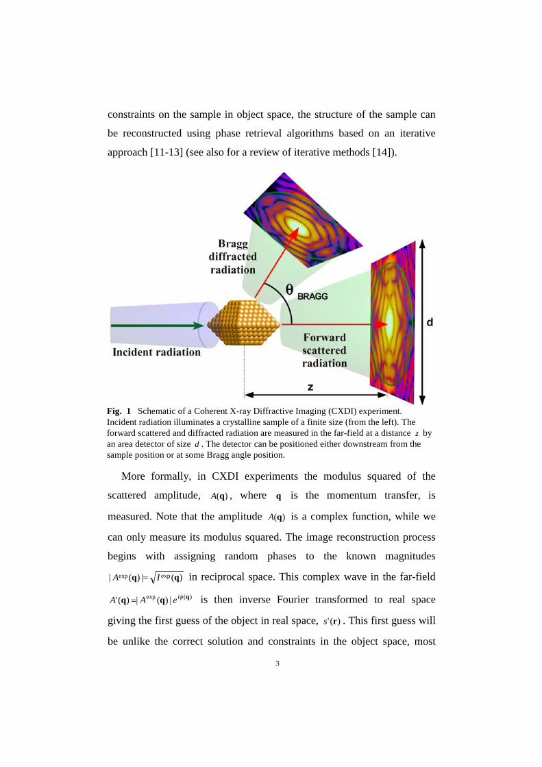
between the sample and detector (see Fig. 1). This differs from

conventional microscopy schemes which use objective lenses to produce

an image of an object. Taking into account the difficulties of producing

lenses at hard X-ray energies that are both highly resolving and efficient,

we see clearly the advantages of so-called 'lensless' microscopy

techniques. After its first demonstration [1-4] CXDI was successfully

applied at 3rd generation synchrotron sources for imaging micron and

nanometer size samples (see for recent reviews [5-10]).

The conventional CXDI experiment is performed with an isolated

sample illuminated by a coherent, plane wave (Fig. 1). The incident wave

may be described by a complex field (with a real and an imaginary part) of

uniform magnitude and phase. The radiation interacts with the sample,

which affects both the amplitude and phase of this field. The scattered

radiation from the sample propagates to a two-dimensional detector in the

far-field, and the diffracted intensities are measured. The detector can be

positioned either in the forward direction, or in the case of a crystalline

sample at Bragg angle positions (Fig. 1). It will be shown in the following

sections that in the limit of kinematical scattering, which is a good

approximation for scattering on nanostructures, the amplitude of the

scattered field can be expressed as the Fourier transform (FT) of the

electron density of a sample. However, the measurement of diffracted

intensities exclusively is insufficient to unambiguously determine the

electron density of a sample, as the phase information is lost during the

measurement process (the measured quantity is the intensity and not the

complex amplitude). Fortunately, with some additional knowledge of

3

constraints on the sample in object space, the structure of the sample can

be reconstructed using phase retrieval algorithms based on an iterative

approach [11-13] (see also for a review of iterative methods [14]).

More formally, in CXDI experiments the modulus squared of the

scattered amplitude, )(qA , where q is the momentum transfer, is

measured. Note that the amplitude )(qA is a complex function, while we

can only measure its modulus squared. The image reconstruction process

begins with assigning random phases to the known magnitudes

)(|)(| expexp qq IA = in reciprocal space. This complex wave in the far-field

)(exp |)(|)(' qqq φieAA = is then inverse Fourier transformed to real space

giving the first guess of the object in real space, )(' rs . This first guess will

be unlike the correct solution and constraints in the object space, most

Fig. 1 Schematic of a Coherent X-ray Diffractive Imaging (CXDI) experiment. Incident radiation illuminates a crystalline sample of a finite size (from the left). The forward scattered and diffracted radiation are measured in the far-field at a distance z by an area detector of size d . The detector can be positioned either downstream from the sample position or at some Bragg angle position.

4

importantly the finite extent of the object, have to be taken into account

for better solutions. This typically involves setting the values of )(' rs

outside some bound to zero, known as the Error Reduction (ER) method,

or forcing them towards zero, most commonly the Hybrid Input-Output

(HIO) method [12]. After the constraints have been applied, the updated

function )(rs is then Fourier transformed to the far-field. The magnitude

|)(| qA of this new far-field guess is replaced by the measured intensities

)(|)(| expexp qq IA = while the phases )(qφ are kept. This process is then

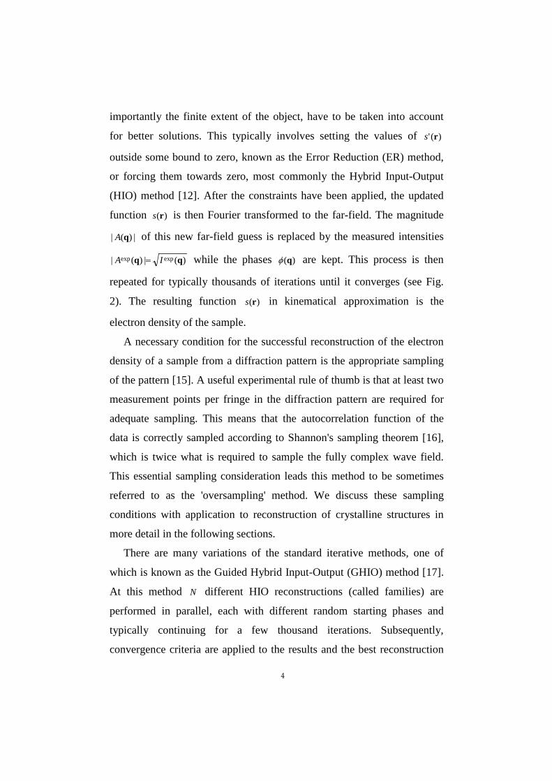
repeated for typically thousands of iterations until it converges (see Fig.

2). The resulting function )(rs in kinematical approximation is the

electron density of the sample.

A necessary condition for the successful reconstruction of the electron

density of a sample from a diffraction pattern is the appropriate sampling

of the pattern [15]. A useful experimental rule of thumb is that at least two

measurement points per fringe in the diffraction pattern are required for

adequate sampling. This means that the autocorrelation function of the

data is correctly sampled according to Shannon's sampling theorem [16],

which is twice what is required to sample the fully complex wave field.

This essential sampling consideration leads this method to be sometimes

referred to as the 'oversampling' method. We discuss these sampling

conditions with application to reconstruction of crystalline structures in

more detail in the following sections.

There are many variations of the standard iterative methods, one of

which is known as the Guided Hybrid Input-Output (GHIO) method [17].

At this method N different HIO reconstructions (called families) are

performed in parallel, each with different random starting phases and

typically continuing for a few thousand iterations. Subsequently,

convergence criteria are applied to the results and the best reconstruction

5

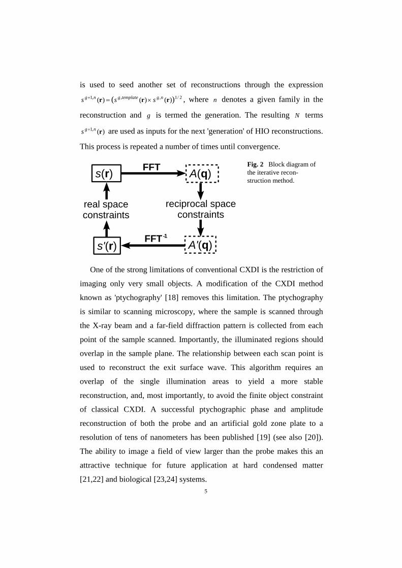
is used to seed another set of reconstructions through the expression 2/1,,,1 )( )()()( rrr ngtemplategng sss ×=+ , where n denotes a given family in the

reconstruction and g is termed the generation. The resulting N terms

)(,1 rngs + are used as inputs for the next 'generation' of HIO reconstructions.

This process is repeated a number of times until convergence.

One of the strong limitations of conventional CXDI is the restriction of

imaging only very small objects. A modification of the CXDI method

known as 'ptychography' [18] removes this limitation. The ptychography

is similar to scanning microscopy, where the sample is scanned through

the X-ray beam and a far-field diffraction pattern is collected from each

point of the sample scanned. Importantly, the illuminated regions should

overlap in the sample plane. The relationship between each scan point is

used to reconstruct the exit surface wave. This algorithm requires an

overlap of the single illumination areas to yield a more stable

reconstruction, and, most importantly, to avoid the finite object constraint

of classical CXDI. A successful ptychographic phase and amplitude

reconstruction of both the probe and an artificial gold zone plate to a

resolution of tens of nanometers has been published [19] (see also [20]).

The ability to image a field of view larger than the probe makes this an

attractive technique for future application at hard condensed matter

[21,22] and biological [23,24] systems.

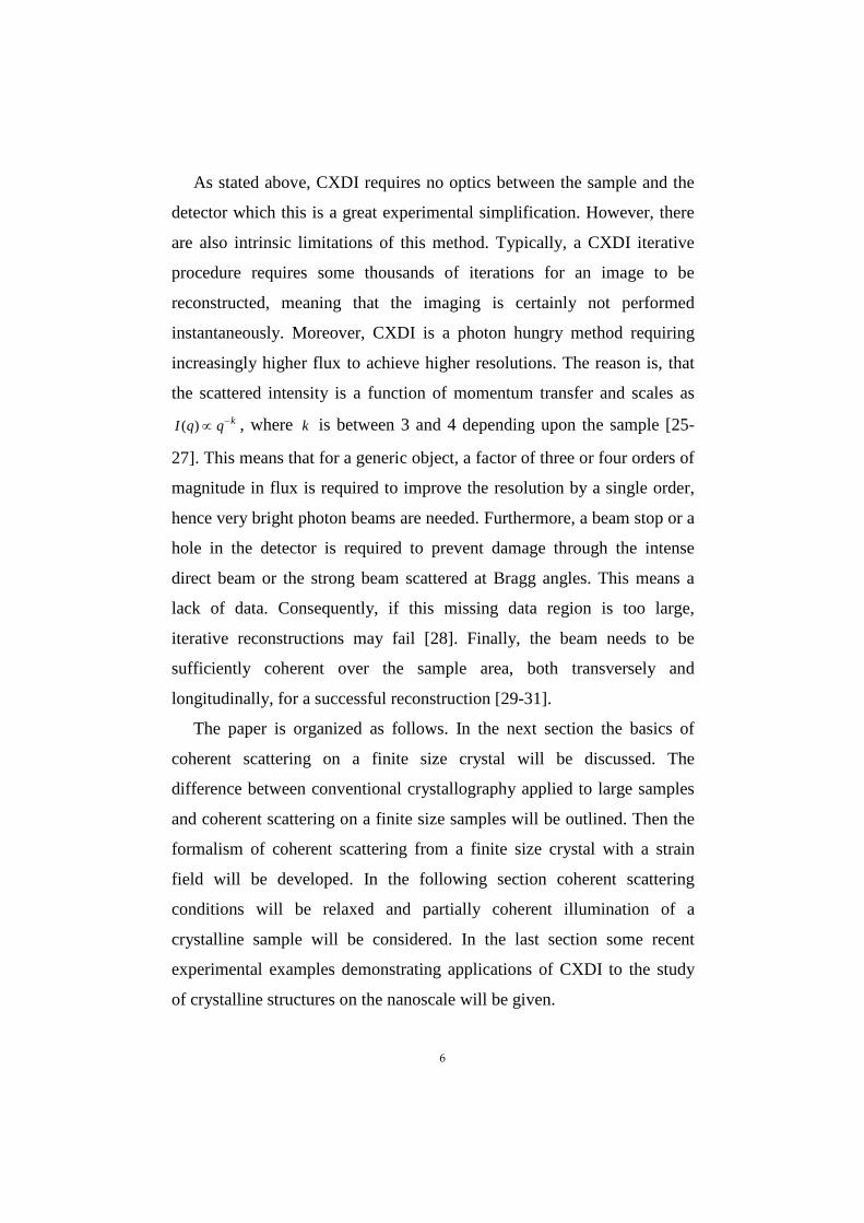
FFT

FFT -1

s(r)

s'(r)

A(q)

real spaceconstraints

reciprocal spaceconstraints

A'(q)

Fig. 2 Block diagram of the iterative recon-struction method.

6

As stated above, CXDI requires no optics between the sample and the

detector which this is a great experimental simplification. However, there

are also intrinsic limitations of this method. Typically, a CXDI iterative

procedure requires some thousands of iterations for an image to be

reconstructed, meaning that the imaging is certainly not performed

instantaneously. Moreover, CXDI is a photon hungry method requiring

increasingly higher flux to achieve higher resolutions. The reason is, that

the scattered intensity is a function of momentum transfer and scales as kqqI −∝)( , where k is between 3 and 4 depending upon the sample [25-

27]. This means that for a generic object, a factor of three or four orders of

magnitude in flux is required to improve the resolution by a single order,

hence very bright photon beams are needed. Furthermore, a beam stop or a

hole in the detector is required to prevent damage through the intense

direct beam or the strong beam scattered at Bragg angles. This means a

lack of data. Consequently, if this missing data region is too large,

iterative reconstructions may fail [28]. Finally, the beam needs to be

sufficiently coherent over the sample area, both transversely and

longitudinally, for a successful reconstruction [29-31].

The paper is organized as follows. In the next section the basics of

coherent scattering on a finite size crystal will be discussed. The

difference between conventional crystallography applied to large samples

and coherent scattering on a finite size samples will be outlined. Then the

formalism of coherent scattering from a finite size crystal with a strain

field will be developed. In the following section coherent scattering

conditions will be relaxed and partially coherent illumination of a

crystalline sample will be considered. In the last section some recent

experimental examples demonstrating applications of CXDI to the study

of crystalline structures on the nanoscale will be given.

7

2. COHERENT AND PARTIALLY COHERENT SCATTERING ON CRYSTALS

The scattering from an isotropic sample and a periodic crystal, when the

intensity peaks at the Bragg positions, is quite different. R. Millane [32]

was first to discuss in detail similarities and differences of the phase

retrieval problem in crystallography and optics. Here we will give a short

overview of this problem extending it to the case of finite size and strained

crystals (see also [29]) where the link with the phase retrieval applied to

non-crystallographic samples will be most evident. We will also discuss

how this problem is connected with Shannon's sampling theorem and the

possibilities of using the results of this theorem for phase retrieval in

crystallography.

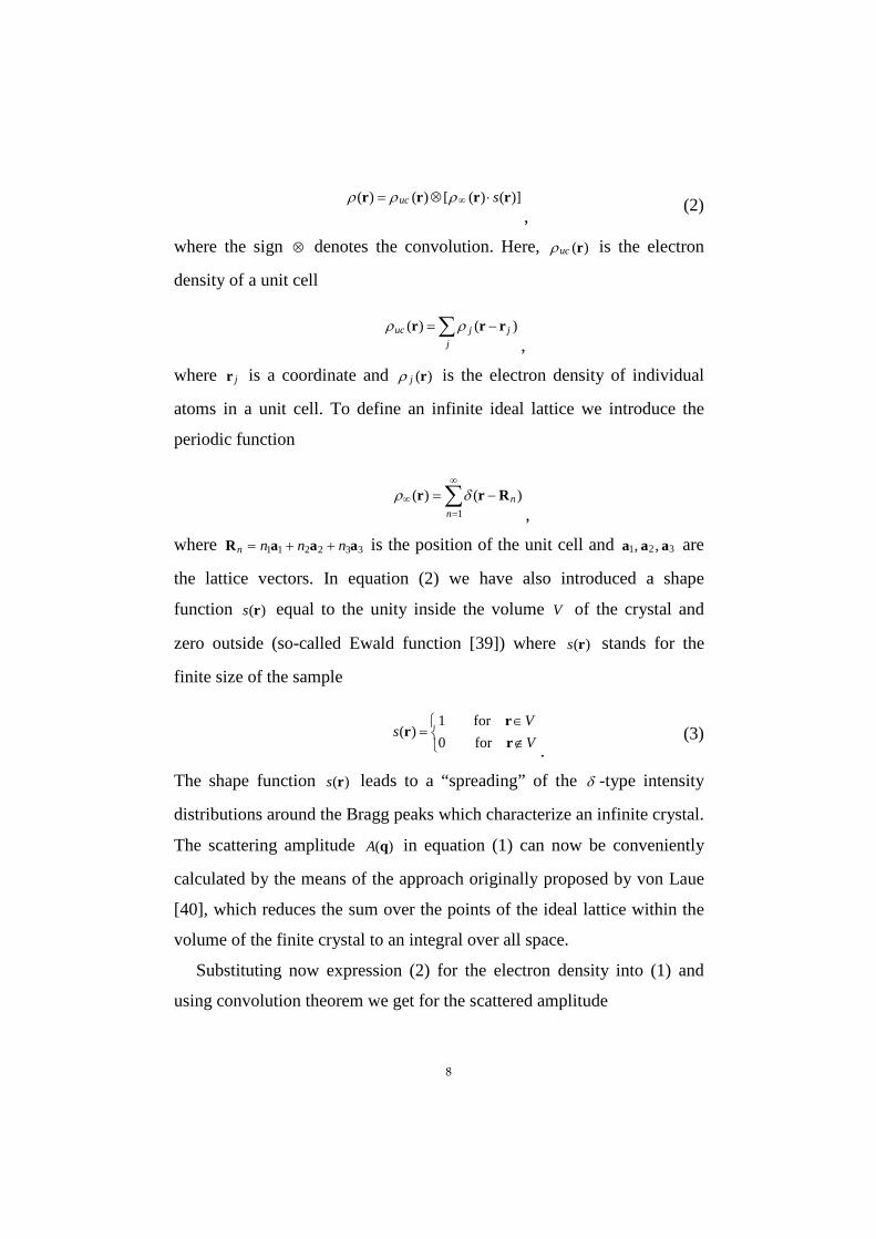
2.1 Coherent scattering from a finite size crystal

It is well known (see for example [33,34]) that the scattering amplitude

)(qA of coherent monochromatic radiation from an infinite crystal in

kinematical approximation1 is equal to

∫ ⋅−= rdeA i 3)()( rqrq ρ

, (1)

where )(rρ is the electron density at the point r , if kkq −= is the

momentum transfer and ik and fk are the incident and scattered wave

vectors ( λπ /2|||| == fi kk , λ is the wavelength). The electron density of a

finite size crystal can be written as

1 Here we assume that the kinematical approximation for the description of X-ray

scattering on crystalline samples is valid. This is a good approximation for scattering of X-rays in the range of 10 keV and submicron crystal sizes. However, if crystalline particles reach few micron size, multiple scattering, or dynamical effects [35,36] could become important [37]. For these crystal sizes refraction effects should be also considered [38].

8

)]()([)()( rrrr suc ⋅⊗= ∞ρρρ

, (2)

where the sign ⊗ denotes the convolution. Here, )(rucρ is the electron

density of a unit cell

∑ −=

jjjuc )()( rrr ρρ

,

where jr is a coordinate and )(rjρ is the electron density of individual

atoms in a unit cell. To define an infinite ideal lattice we introduce the

periodic function

∑∞

=∞ −=

1

)()(n

nRrr δρ,

where 332211 aaaR nnnn ++= is the position of the unit cell and 321 ,, aaa are

the lattice vectors. In equation (2) we have also introduced a shape

function )(rs equal to the unity inside the volume V of the crystal and

zero outside (so-called Ewald function [39]) where )(rs stands for the

finite size of the sample

∉∈

=VV

srr

rfor0for1

)(.

(3)

The shape function )(rs leads to a “spreading” of the δ -type intensity

distributions around the Bragg peaks which characterize an infinite crystal.

The scattering amplitude )(qA in equation (1) can now be conveniently

calculated by the means of the approach originally proposed by von Laue

[40], which reduces the sum over the points of the ideal lattice within the

volume of the finite crystal to an integral over all space.

Substituting now expression (2) for the electron density into (1) and

using convolution theorem we get for the scattered amplitude

9

)()()()( qqqq sFA ⊗⋅= ∞ρ.

(4)

Here

∑∫ ⋅−⋅− ==

j

ij

iuc

jefrdeF rqrq qrq )()()( 3ρ

(5)

is the structure factor of the unit cell and

rdef ijj

3)()( rqrq ⋅−∫= ρ

(6)

is the atomic scattering factor of the atom j in the unit cell and integration

is performed over the volume of the unit cell. It is also assumed that the

structure factors of the different cells are identical, as it is in general for

perfect crystals. Usually, the structure factor )(qF is a complex function.

In equation (4)

rdess i 3)()( rqrq ⋅−∫=

(7)

is the Fourier transform of the shape function )(rs and )(q∞ρ is the

Fourier transform of the lattice function that reduces to the sum of δ -

functions

∑∫ −== ⋅−

∞∞n

ni

vrde )()2()()(

33 hqrq rq δπρρ

, (8)

where v is the volume of the unit cell, 321 hhhh lkhn ++= being the

reciprocal lattice vectors and the summation is carried out over all

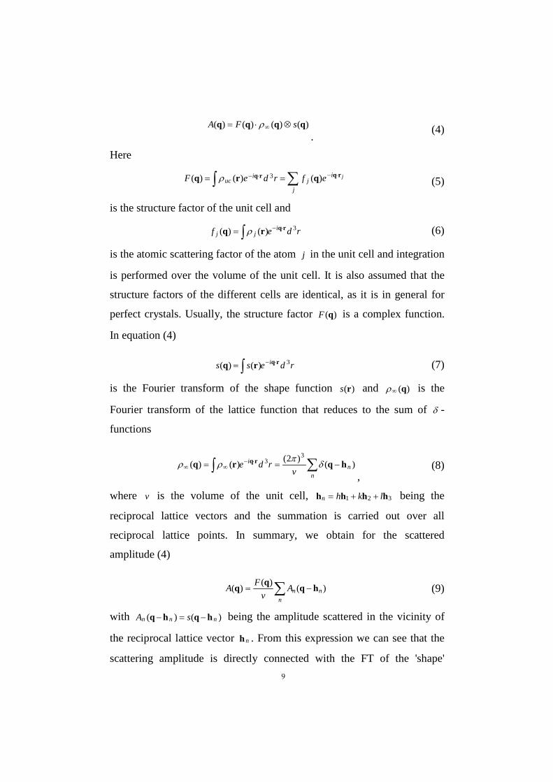
reciprocal lattice points. In summary, we obtain for the scattered

amplitude (4)

∑ −=

nnnA

vFA )()()( hqqq

(9)

with )()( nnn sA hqhq −=− being the amplitude scattered in the vicinity of

the reciprocal lattice vector nh . From this expression we can see that the

scattering amplitude is directly connected with the FT of the 'shape'

10

function )(rs . Here it is also important to note that the structure factor

)(qF is extended in reciprocal space over many reciprocal lattice points. In

the limit of the infinite crystal FT of the shape function )(qs (7) reduces to

the δ -function and we get for the amplitude (9)

∑ −=

nnv

FA )()()( hqqq δ.

(10)

It is a well-known result in crystallography that the scattering amplitude of

the infinite periodic object is sampled at its reciprocal lattice or Bragg

points and, in principle, no information is available between these

sampling points. Taking the inverse FT of (10) we obtain a well known

crystallographic formula for the electron density of the unit cell expressed

through the Fourier components of structure factors

∑ ⋅=

n

nin eF

vh

rhhr )(1)(ρ.

(11)

Unfortunately, only the amplitudes |)(| nF h of the structure factors can be

measured in experiment and there is no direct phase information available

(so-called phase problem in crystallography).

For a crystal of macroscopic dimensions aD >> , where a is the size of

a unit cell, the function )(qs has appreciable values only for Dq /2~ π∆

much smaller than the reciprocal lattice parameters nahn )/2( π= . Thus

according to (9) and neglecting the small cross terms, the intensity

scattered by the crystal of finite dimensions will be determined by the sum

over reciprocal lattice points

∑ −==

nnnA

vF

AI 22

22 |)(|

)(|)(|)( hq

qqq

. (12)

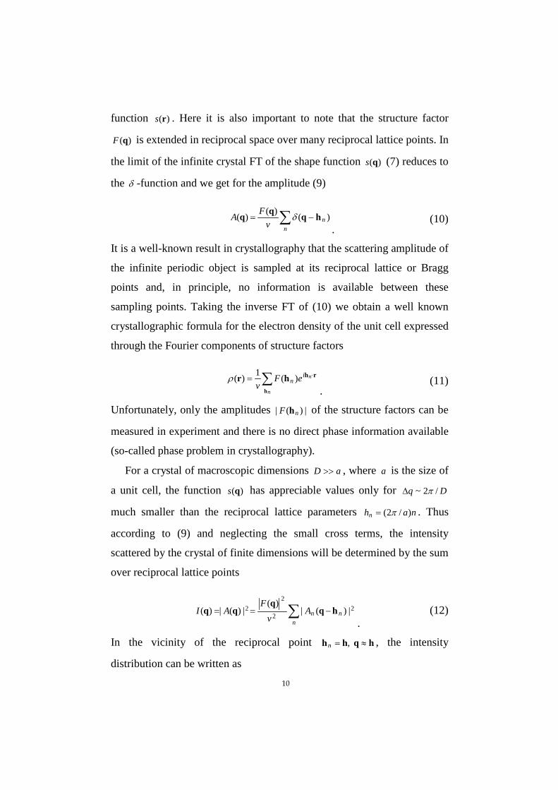
In the vicinity of the reciprocal point hqhh ≈= ,n , the intensity

distribution can be written as

11

2

2

2|)(||)(|)( QhQ hh A

vFI =

, (13)

where hqQ −= and )()( QQ hh sA = .

In the case of the infinite crystal we have from (10)

∑ −==

nn

v

FAI )(

)(|)(|)( 2

22 hq

qqq δ

. (14)

According to this mathematics, several important points have to be

outlined. First of all, according to (10) and (14) in the case of the infinite

crystal the scattering amplitude (or structure factor of the unit cell), and

thus the intensity, is sampled at fixed points in reciprocal space. These

points correspond to the nodes of the reciprocal lattice nh . Generally, no

experimental information is available in between these sampling points

and there is no way to measure continuous diffraction patterns from

infinite crystal. Hence, there is no possibility to oversample diffraction

patterns from infinite crystals. This was noted first by D. Sayre [41] in

early 50-s. It was also noted by the same author that sampling of the

reciprocal space at Bragg points corresponds exactly to Nyquist sampling

of the electron density of the unit cell of size a (for simplicity we will

limit our discussion with 1D case). In other words, if we have an infinite

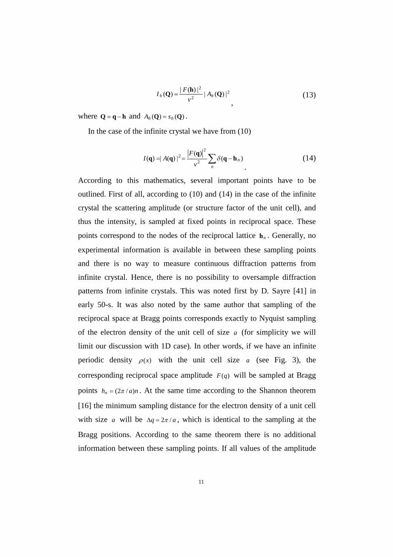
periodic density )(xρ with the unit cell size a (see Fig. 3), the

corresponding reciprocal space amplitude )(qF will be sampled at Bragg

points nahn )/2( π= . At the same time according to the Shannon theorem

[16] the minimum sampling distance for the electron density of a unit cell

with size a will be aq /2π=∆ , which is identical to the sampling at the

Bragg positions. According to the same theorem there is no additional

information between these sampling points. If all values of the amplitude

12

)(qF at the sampling points are known then a continuous amplitude could

be constructed uniquely as

∑ −

−=

nh n

nn hq

hqahFa

qF)(

)](2/sin[)(2)(π

π

. (15)

If the complex structure factors )( nhF (including the phases) could be

measured it would be possible to construct a continuous function )(qF

according to 15). Then, applying the inverse FT, the electron density in the

unit cell could be reconstructed. However, as mentioned above the phases

of )( nhF are missing in the measurements. So, in the case of the infinite

periodic sample it appears impossible to obtain a continuous diffraction

pattern and consequently to apply an oversampling method for phase

retrieval methods. Situation looks even worse when the intensity

distribution )(qI (14) is analyzed: The intensity distribution can be

presented as a FT of the autocorrelation function of the electron density.

For the electron density of the unit cell of size a , the corresponding

autocorrelation function would have an extension of a2 with

corresponding minimum Nyquist sampling frequency aq /π=∆ . That

means that we cannot make use of the sampling theorem (15) to

Fig. 3 (a) Periodic electron density )(xρ with the unit cell size a . (b) Due to a periodicity of the electron density structure factor )(qF is sampled at Bragg points

nahn )/2( π= . No additional data points can be measured in between these sampling points, so in traditional crystallography oversampling is not possible.

13

reconstruct continuous intensity distribution function )(qI , because just

half of the necessary data points are missing. As a consequence phase

problem in crystallography is twice underdetermined. That makes phase

retrieval for crystallography even more difficult problem then in optics.

The situation is quite different if, instead of an infinite crystal, a crystal

of finite size is illuminated with coherent beams. Then the intensity

distribution is given by (12) and is therefore the FT of a shape function

)(rs around each of the Bragg points. It is clear that in this case the

intensity distribution around each Bragg point will be a continuous

function and can be, in principle, oversampled to necessary level. Hence, a

unique reconstruction of the crystal shape is possible.

Some general properties of this intensity distribution have to be

outlined. For an arbitrary shap of the unstrained crystal, the intensity

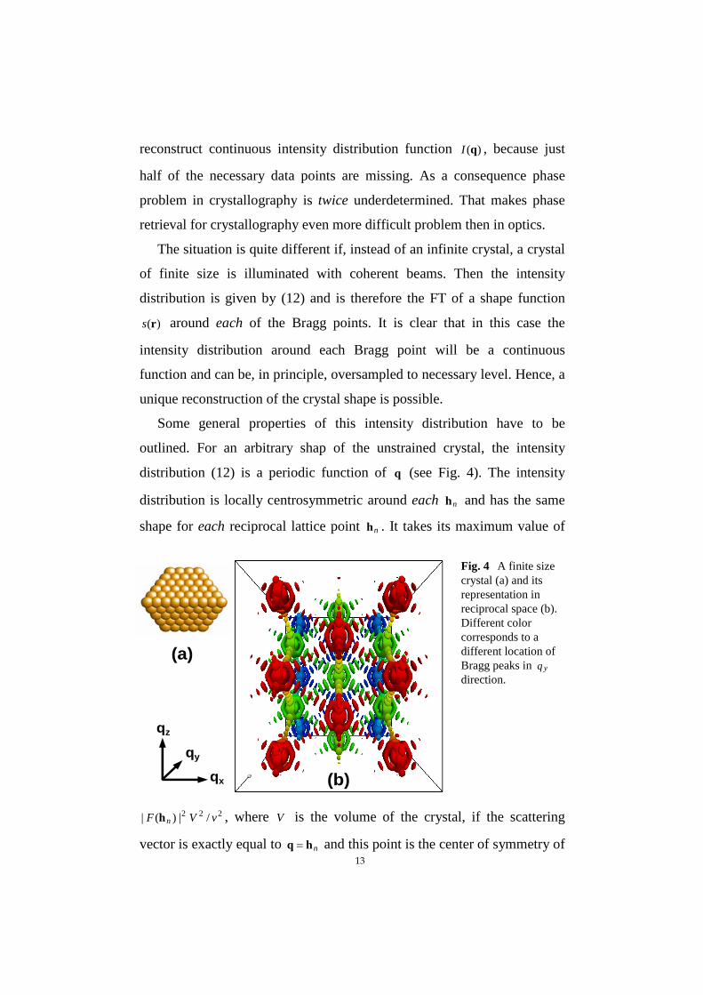
distribution (12) is a periodic function of q (see Fig. 4). The intensity

distribution is locally centrosymmetric around each nh and has the same

shape for each reciprocal lattice point nh . It takes its maximum value of

222 /|)(| vVF nh , where V is the volume of the crystal, if the scattering

vector is exactly equal to nhq = and this point is the center of symmetry of

qx

qz

qy

(a)

(b)

Fig. 4 A finite size crystal (a) and its representation in reciprocal space (b). Different color corresponds to a different location of Bragg peaks in yq direction.

14

the intensity distribution )(qI (since according to (7) )()( qq ∗=− ss ). As

follows from equation (12) the simplest picture of identical repeated

distributions arises in unstrained crystals of any arbitrary shape. The

detailed 3D shape of this distribution is determined by the FT of the

crystal shape function )(rs (see Eq.(7)). The intensity distribution

measured by the 2D detector depends also on the Bragg angle and on the

deviation from the exact Bragg conditions (the detector plane is always

perpendicular to fk vector). If the z -axis in reciprocal space is directed

along the fk vector and the detector is positioned at a Bragg angle, then

we have from Eqs. (7) to (13) the following distribution of the amplitude

in reciprocal space

dxdyeyxs

vFQQA yiQxiQ

zyxyx∫ −−= ),()(),( h

, (16)

where dzzyxsyxsz ),,(),( ∫= is the projection of the crystal shape on the

),( yx -plane that is defined as perpendicular to the fk vector. Obviously,

the inverse FT of the amplitude distribution ),( yx QQA will recover this

projection of the crystal shape. It is also clear that for a general crystalline

sample this projection is equivalent to the projection of the electron

density of a sample to the same plane.

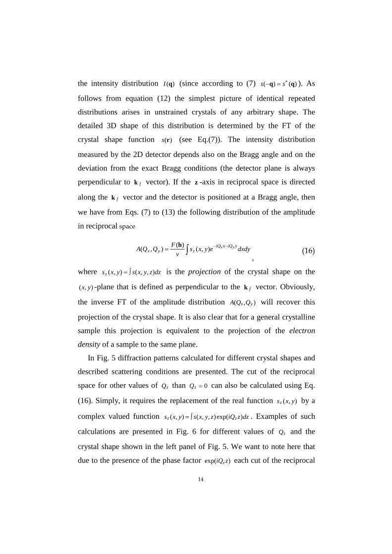
In Fig. 5 diffraction patterns calculated for different crystal shapes and

described scattering conditions are presented. The cut of the reciprocal

space for other values of zQ than 0=zQ can also be calculated using Eq.

(16). Simply, it requires the replacement of the real function ),( yxsz by a

complex valued function dzziQzyxsyxs zz )exp(),,(),( ∫= . Examples of such

calculations are presented in Fig. 6 for different values of zQ and the

crystal shape shown in the left panel of Fig. 5. We want to note here that

due to the presence of the phase factor )exp( ziQz each cut of the reciprocal

15

space by the Ewald sphere at 0≠zQ will produce non-centrosymmetric

intensity distribution even for an unstrained crystal (see Fig. 6). However,

the 3D intensity distribution will be centrosymmetric around each Bragg

point (see Fig. 4).

In principle, the whole 3D intensity distribution )(QI can be measured

by a 2D detector and by scanning the sample near Bragg position or

changing the incident energy. This 3D distribution can also be directly

inverted giving the shape of the crystalline part of the sample in 3D (see

for the first demonstration [42]). Remarkably, in the case of the 3D phase

retrieval the necessary conditions on oversampling in the third dimension

are quite relaxed as was noted by Millane [43]. In practice, few tens of

angular scans in reciprocal space are sufficient to invert the 3D diffraction

pattern of a micron size crystalline particle (see for details [42,44]).

As was proposed by von Laue [40] the Green's theorem can be applied

to Eq. (7) and the volume integral can be transformed to an integral over

the external surface area ( S ) of the crystal

∫ ⋅−⋅=S

i deqis σrqnqq )()( 2

, (17)

where the unit vector n is an outward normal to the crystal. The maximum

of this distribution for the flat surface is along directions normal to the

surface. The existence of these flares was predicted by von Laue [40] and

given the name “Stacheln” (spike). They have been experimentally

Fig. 5 Projection of the different crystal shapes on the plane perpendicular to fk and corresponding diffraction pattern calculated at exact the Bragg position. Adapted from Ref. [29].

16

observed later in the studies of the surface diffraction in the form of

crystal truncation rods (CTR) [45], or asymptotic Bragg diffraction [46].

In the case of a crystal with a center of symmetry and with a pair of

identical opposite facets we obtain from (17)

∫ ⋅

⋅=

Sd

qs σ)sin()(2)( 2 rqnqq

. (18)

If the distance between the facets is equal to D , then for the direction of q

perpendicular to the facets we finally get

)2/sin(2)( qDSq

qs =.

(19)

It follows immediately, that for two opposite facets and coherent

illumination interference patterns appear in the intensity distribution rather

than a smooth 2−q decrease of intensity for a single surface (see Fig. 5).

This interference pattern is similar to the fringes from slit scattering in

optics, when the slit is illuminated by a coherent light. The integral width

of this intensity distribution in reciprocal space is equal to Dq /2πδ = . This

leads to a rod-like shape intensity distribution for crystals shaped like a

compressed disc. Such behavior was, for example, observed in the study

of thin films of AuCu3 [47]. In the case of a flat surface the same Green's

theorem can be applied once more to equation (17) transforming the

surface integral to an integral around the boundary of the facet S . Now,

(a) (b) (c) (d)

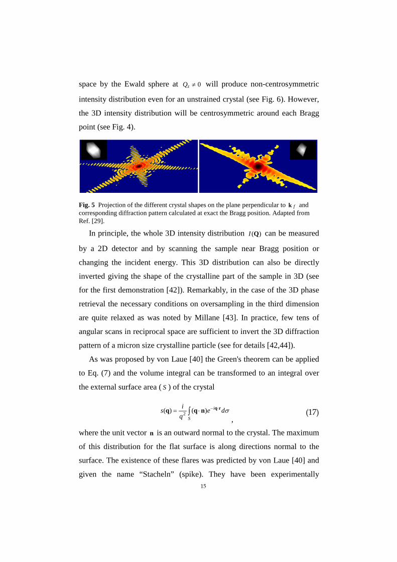
Fig. 6 The cross section of the reciprocal space of the diffraction pattern calculated from the crystal shape shown in the inset of Fig. 12.5 (left panel) for different zq values: (a)

0=zq , (b) Dz qq 357.0= , (c) Dz qq 476.0= and (d) Dz qq 19.1= . Here Dq correspond to the fringe spacing DqD /2~ π . Intensity in figure is rescaled for clarity. Adapted from Ref. [29].

17

diffraction from the edges will produce, instead of truncation rods, crystal

truncation planes (CTP) (see for the first observation of CTP [48]).

As a conclusion we can summarize that any pair of opposite facets and

corresponding edges of unstrained crystals in a coherent beam produces an

interference pattern with the maximum intensity distribution along the

normal to the facet (CTR), or perpendicular to the opposite surface edges

(CTP).

Equation (12) corresponds to the situation when one particle is

illuminated by a coherent beam. In the case when two or more crystallites

are located at some distance from each other and are illuminated by the

same coherent beam additional interference terms will appear in the

expression for the intensity (12). Especially interesting (but not discussed

here) is the case when a small particle is well separated from a big one and

illuminated by the same coherent beam. This is similar to the principles of

Fourier holography, when the object can be found as one term in the

autocorrelation [49-51].

Up to now we presented the mathematics of diffraction patterns which

are measured locally around a fixed Bragg point for a crystal of the finite

size. However, another kind of measurement can be suggested, when

diffraction patterns are measured simultaneously around several reciprocal

lattice points. Taking into account that this distribution is measured for a

finite number of reciprocal lattice points up to max~ qq the complex

amplitude distribution can be written as

[ ])()()()()( qqqqq sFBA ⊗⋅⋅= ∞ρ, (20)

where )(qB is an envelope function with the effective size max~ qq . Inverting

this relationship with the inverse FT yields in real space an electron density

18

)]()([)]()([)( rrrrr sb uc ⋅⊗⊗= ∞ρρρ,

(21)

where )(rb is the inverse Fourier transform of )(qB . This electron density

is peaking at the regular positions of the unit cell due to the function )(r∞ρ

and has an overall shape of the sample )(rs . Most importantly, it contains

the position of the atoms in the unit cell due to the reconstruction of the

electron density function of a unit cell )(rucρ . This means the following: If

the continuous intensity distribution around several Bragg peaks will be

measured simultaneously and phase retrieval methods will be applied to

get the phase, then, in principle, the electron density with atomic

resolution will be obtained. The resolution in real space around each

atomic position in such experiments will be determined by the area

accessed in the measurements in reciprocal space and can be estimated to

be about max/2~ qr π∆ .

In order to map several Bragg peaks simultaneously with one detector

different approaches can be applied. For conventional crystalline samples

with a unit cell of the size of a few angstroms hard X-rays in the range of

100 keV should be used [52]. Another approach is to use long period

crystalline samples such as colloidal crystals with a typical unit cell sizes

on the order of a few hundred nanometers. The latter was successfully

realized in CXDI experiments on colloidal 2D and 3D samples [53,54]

(see section 3.1 ). High energy electron beams in nano-diffraction

experiments with the conventional transmission electron microscope

(TEM) can be also used for realization of these ideas [55-57].

2.2 Coherent scattering from a finite size crystal with a strain

In the case of a deformed crystal we can write the electron density as the

sum of terms corresponding to individual atoms

19

( )∑∑

= =

−−=N

n

S

jnjnjnj

1 1

)()( RuRrr ρρ,

(22)

where jnnj rRR += and )( njRu is the displacement from the ideal lattice

point. Summation in (22) is performed over N unit cells which contain S

atoms. We assume here that the whole crystal is coherently illuminated.

Substituting this expression for the electron density into (1) and changing

variables in each term, the scattering amplitude can be written as a sum

over the unit cells

∑=

⋅−⋅−=N

n

iin

nn eeFA1

)()()( RqRuqqq,

(23)

where )(qnF is the complex valued structure amplitude of the nth cell. Here

it is assumed that all atoms in the unit cell are displaced uniformly

)()()( njnnj RurRuRu =+≡ . It is important to note that equation (23) is also

valid for the more general case allowing different displacements of atoms

in different unit cells but with another definition of the structure amplitude

)(qnF [58].

Now we will consider, as before, the scattering of X-rays on a crystal

with finite size. The scattering amplitude )(qA (23) for the crystal of finite

dimensions will be calculated using the same approach as described in the

previous section. According to this approach equation (23) can be

identically rewritten in the form

∫ ⋅−∞= rdeSFA i 3)()()()( rqrrqq ρ

, (24)

where it is assumed that the structure factors of the different cells are

identical with )()( qq FFn = and integration is carried out over the whole

space. In this equation we have introduced a complex function

20

( ))(exp)()( ruqrr ⋅−= isS

(25)

with the shape function )(rs (3) as an amplitude and the phase

)()( ruqr ⋅=φ , where the deformation field )(ru is included. It is important

to note that no restrictions on the shape of the crystal and the deformation

field apply.

Performing now the same calculations as in the previous section we

will obtain for the amplitude (see Eq. (4))

)()()()( qqqq ∞⊗⋅= ρSFA,

(26)

where )(qS is the Fourier integral of )(rS

rdeSS i 3)()( rqrq ⋅−∫=

, (27)

and the integration over rd 3 is carried out over the whole space.

Now using the expression for the FT of )(r∞ρ (8) we can derive the

amplitude (26)

∑ −=

nnnA

vFA )()()( hqqq

, (28)

with )()( nnn SA hqhq −=− , now containing the deformation values. From

this expression we can see that the scattering amplitude is directly

connected with the FT of the complex 'shape' function )(rS and its phase

for the fixed reciprocal lattice point h is a sum of phases of the structure

factor )(hF and function )(qS .

For a crystal of macroscopic dimensions we will again get a periodic

intensity distribution

∑ −==

nnnA

vFAI 22 |)(|)(|)(|)( hqqqq

, (29)

where each term gives intensity values close to reciprocal point,

21

2

2

2|)(||)(|)( QhQ hA

vFIh =

. (30)

Here the amplitudes )(QhA are defined as

∫ ⋅−⋅−= rdeesA ii 3)()()( rQruh

h rQ,

(31)

and as before hqQ −= .

In the following we will outline the differences between the coherent

diffraction pattern of the unstrained crystal and the crystal with the

deformation field. In this case for any arbitrary form of the crystal and the

strain field, the intensity distribution (29) is still localized around

reciprocal lattice vectors nh . However, in contrast to the unstrained case,

for samples with arbitrary strain the intensity distribution locally is not

centrosymmetric around nh and the shape differs at every reciprocal

lattice point nh . Effects associated with the strain )(ru lead to different

distributions near different reciprocal-lattice points.

This is illustrated in Fig. 7, where a two-dimensional example of the

diffraction from a strained object is shown. In Fig. 7(a) a real envelope

function )(rs , defining a crystal shape is shown. It is obtained from a

scanning-electron microscope image of a partially annealed array of gold

nanocrystals on a glass substrate. In Fig. 7(b) its Fourier transform, which

shows the expected local symmetry is depicted. Fig. 7(c) is a

representation of a complex envelope function )(rS , where the amplitude

is the same as before and the phase varies quadratically as a function of

the radius from the object’s center. The shaped (gray) rings represent

phase reversals. The FT (Fig. 7(d)) shows the diffraction pattern expected

from such a strained particle. Clearly, the local symmetry of the unstrained

case on the left is distorted but still the main features, the flares and the

fringes are resembled. This example shows the main point of our

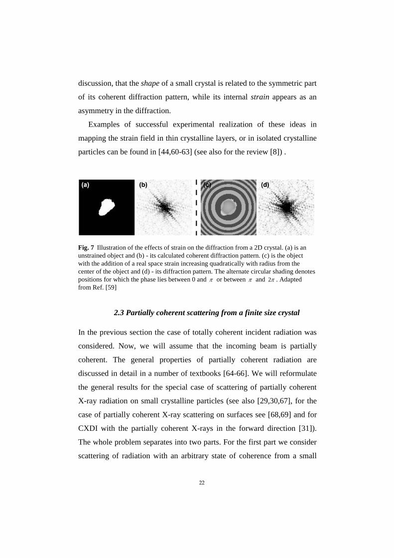
22

discussion, that the shape of a small crystal is related to the symmetric part

of its coherent diffraction pattern, while its internal strain appears as an

asymmetry in the diffraction.

Examples of successful experimental realization of these ideas in

mapping the strain field in thin crystalline layers, or in isolated crystalline

particles can be found in [44,60-63] (see also for the review [8]) .

2.3 Partially coherent scattering from a finite size crystal

In the previous section the case of totally coherent incident radiation was

considered. Now, we will assume that the incoming beam is partially

coherent. The general properties of partially coherent radiation are

discussed in detail in a number of textbooks [64-66]. We will reformulate

the general results for the special case of scattering of partially coherent

X-ray radiation on small crystalline particles (see also [29,30,67], for the

case of partially coherent X-ray scattering on surfaces see [68,69] and for

CXDI with the partially coherent X-rays in the forward direction [31]).

The whole problem separates into two parts. For the first part we consider

scattering of radiation with an arbitrary state of coherence from a small

Fig. 7 Illustration of the effects of strain on the diffraction from a 2D crystal. (a) is an unstrained object and (b) - its calculated coherent diffraction pattern. (c) is the object with the addition of a real space strain increasing quadratically with radius from the center of the object and (d) - its diffraction pattern. The alternate circular shading denotes positions for which the phase lies between 0 and π or between π and π2 . Adapted from Ref. [59]

23

crystalline particle. For the second part a special realization of the

incoherent source with a Gaussian intensity distribution will be discussed.

Let us assume the incident radiation to be a quasi-monochromatic wave

with one polarization state of the electric field,

tiiinin ietAtE ω−⋅= rkrr ),(),(

, (32)

where λπ /2|| =k . Here λ and ω are the average wavelength and

frequency of the beam. The amplitude ),( tAin r is a slowly varying function

with spatial variations much bigger than the wavelength λ and time scales

much larger than ω/1 . Consequently, according to the standard Huygens-

Fresnel principle [64] in the limits of kinematical scattering, the amplitude

of the wavefield ),( tEout v , after being scattered from the sample to

position v at the detector (see Fig. 8), can be written as2

∫ −−⋅−

= rdeltAtE ri ti

r

rinout

3)(),()(),( τωτρ rkrrv

, (33)

where rl is the distance between points r and v with the origins in the

sample center and detector plane respectively, clrr /=τ is the time delay

for the radiation propagation between these points and c is the speed of

light. In this expression for the scattered wavefield we have neglected the

absorption as the small sample is small and set the obliquity factor to

unity.

2 In this expression and below we will omit all not essential integral prefactors.

24

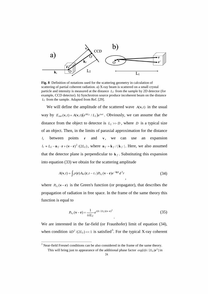
We will define the amplitude of the scattered wave ),( tA v in the usual

way by tiikLout eLetAtE ω)( 2/),(),( 2vv = . Obviously, we can assume that the

distance from the object to detector is DL >>2 , where D is a typical size

of an object. Then, in the limits of paraxial approximation for the distance

rl between points r and v , we can use an expansion

)2/()( 22

2 LLl fr rvrn −+⋅−≈ , where ||/ fff kkn = . Here, we also assumed

that the detector plane is perpendicular to fk . Substituting this expansion

into equation (33) we obtain for the scattering amplitude

∫ ⋅−−−= rdePtAtA iLrin

3)(),()(),( 2rqrvrrv τρ

, (34)

where )(2 rv −LP is the Green's function (or propagator), that describes the

propagation of radiation in free space. In the frame of the same theory this

function is equal to

222

))(2/(

2

1)( rvrv −=− LkiL e

LiP

λ . (35)

We are interested in the far-field (or Fraunhofer) limit of equation (34),

when condition 1)2/( 22 <<LkD is satisfied3. For the typical X-ray coherent

3 Near-field Fresnel conditions can be also considered in the frame of the same theory.

This will bring just to appearance of the additional phase factor ])2/(exp[ 22 rLki in

Fig. 8 Definition of notations used for the scattering geometry in calculation of scattering of partial coherent radiation. a) X-ray beam is scattered on a small crystal particle and intensity is measured at the distance 2L from the sample by 2D detector (for example, CCD detector). b) Synchrotron source produce incoherent beam on the distance

1L from the sample. Adapted from Ref. [29].

25

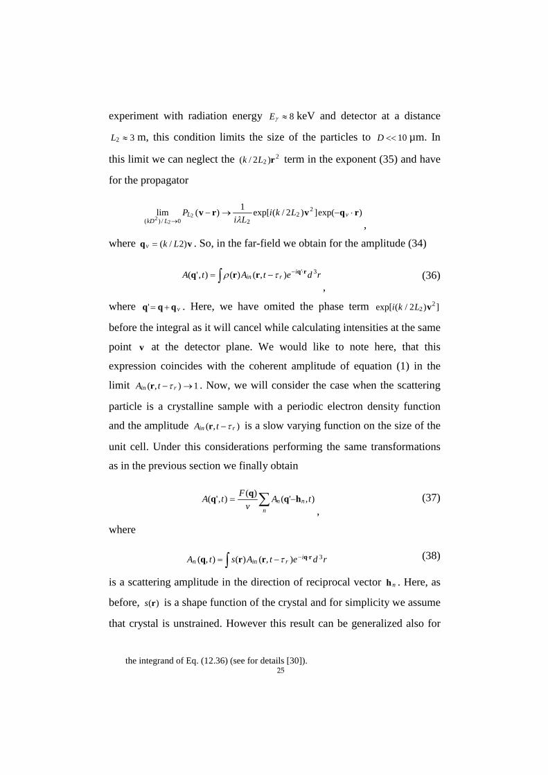
experiment with radiation energy 8≈γE keV and detector at a distance

32 ≈L m, this condition limits the size of the particles to 10<<D µm. In

this limit we can neglect the 22 )2/( rLk term in the exponent (35) and have

for the propagator

)exp(])2/(exp[1)(lim 2

220/)(

222

rqvrv ⋅−→−→

vLLkD

LkiLi

Pλ ,

where vq )2/( Lkv = . So, in the far-field we obtain for the amplitude (34)

∫ ⋅−−= rdetAtA irin

3'),()(),'( rqrrq τρ,

(36)

where vqqq +=' . Here, we have omited the phase term ])2/(exp[ 22 vLki

before the integral as it will cancel while calculating intensities at the same

point v at the detector plane. We would like to note here, that this

expression coincides with the coherent amplitude of equation (1) in the

limit 1),( →− rin tA τr . Now, we will consider the case when the scattering

particle is a crystalline sample with a periodic electron density function

and the amplitude ),( rin tA τ−r is a slow varying function on the size of the

unit cell. Under this considerations performing the same transformations

as in the previous section we finally obtain

∑ −=

nnn tA

vFtA ),'()(),'( hqqq

, (37)

where

∫ ⋅−−= rdetAstA i

rinn3),()(),( rqrrq τ

(38)

is a scattering amplitude in the direction of reciprocal vector nh . Here, as

before, )(rs is a shape function of the crystal and for simplicity we assume

that crystal is unstrained. However this result can be generalized also for

the integrand of Eq. (12.36) (see for details [30]).

26

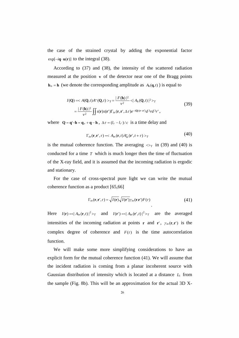
the case of the strained crystal by adding the exponential factor

)](exp[ ruq ⋅−i to the integral (38).

According to (37) and (38), the intensity of the scattered radiation

measured at the position v of the detector near one of the Bragg points

hh =n (we denote the corresponding amplitude as ),( tAh q ) is equal to

∫∫ −⋅−

∗

∆Γ=

><=>=<

'),',()'()(|)(|

|),(||)(|),(),()(

33)'(2

2

22

2

rrddessv

F

tAv

FtAtAI

iin

ThT

rrQrrrrh

QhQQQ

τ , (39)

where hqqhqQ −+=−= v' , cll rr /)( '−=∆τ is a time delay and

Tininin tAtA >+=<Γ ∗ ),'(),(),',( ττ rrrr

(40)

is the mutual coherence function. The averaging T<> in (39) and (40) is

conducted for a time T which is much longer then the time of fluctuation

of the X-ray field, and it is assumed that the incoming radiation is ergodic

and stationary.

For the case of cross-spectral pure light we can write the mutual

coherence function as a product [65,66]

)()'.()'()(),',( τγτ FII inin rrrrrr =Γ.

(41)

Here Tin tAI >=< 2|),(|)( rr and Tin tAI >=< 2|),'(|)'( rr are the averaged

intensities of the incoming radiation at points r and 'r , )',( rrinγ is the

complex degree of coherence and )(τF is the time autocorrelation

function.

We will make some more simplifying considerations to have an

explicit form for the mutual coherence function (41). We will assume that

the incident radiation is coming from a planar incoherent source with

Gaussian distribution of intensity which is located at a distance 1L from

the sample (Fig. 8b). This will be an approximation for the actual 3D X-

27

ray source from the synchrotron storage ring. We will also consider that

the distance 1L is much larger than the size of the particle D and, than the

average size of the source S . According to the van Cittert-Zernike

theorem [65,66], the complex degree of coherence can be obtained in the

same limit of paraxial approximation (see [70] for the generalization of

this approach)

∫∫ −⋅

=sdI

sdeIe Lkii

in 3

3/)'(

)(

)()',(

1

ss

rrrrsψ

γ,

(42)

where the phase factor is )')(2/( 221 rrLk −=ψ , )(sI is the intensity

distribution of the incoherent source and integration is performed over the

whole area of the incoherent source. It is interesting to note here that for

an incoherent source expression (42) is exact up to second order terms in

s . For the typical CXD experiment at a synchrotron source with a distance

from source to sample 401 ≈L m and an energy of 8≈γE keV the far-field

conditions 1)2( 12 <<LkD can easily be satisfied, giving the upper limit for

the size of the particle as 40<<D µm. In this far-field limit we can neglect

the phase prefactor ψie in Eq. (42) and consider the complex degree of

coherence )',( rrinγ (42) as a real valued function. Following this model of

an incoherent source in the far-field limit the intensity of the incoming

radiation at points r and 'r at the sample can be calculated as:

sdILIII 2210 )()/()'()( srr ∫==≈ λ .

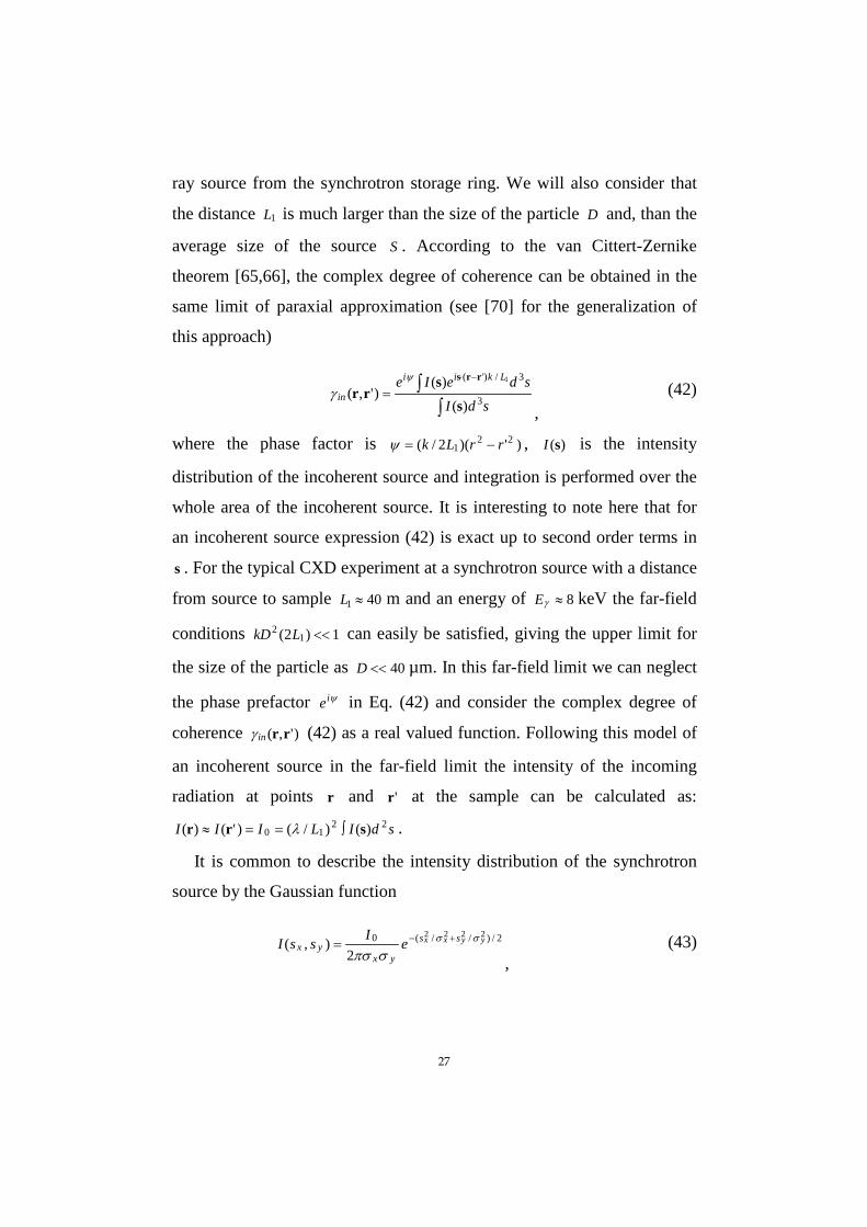
It is common to describe the intensity distribution of the synchrotron

source by the Gaussian function

2/)//(0 2222

2),( yyxx ss

yxyx eIssI σσ

σπσ+−=

, (43)

28

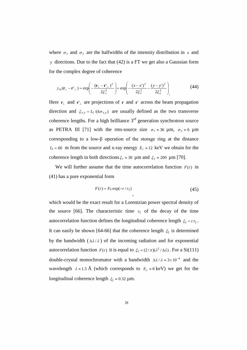
where xσ and yσ are the halfwidths of the intensity distribution in x and

y directions. Due to the fact that (42) is a FT we get also a Gaussian form

for the complex degree of coherence

−−

−−=

−−=−

⊥

⊥⊥⊥⊥ 2

2

2

2

2

2

2)'(

2)'(exp

2)'(exp)'(

yxin

yyxxξξξ

γ rrrr.

(44)

Here ⊥r and ⊥'r are projections of r and 'r across the beam propagation

direction and )/( ,1, yxyx kL σξ = are usually defined as the two transverse

coherence lengths. For a high brilliance 3rd generation synchrotron source

as PETRA III [71] with the rms-source size 36≈xσ µm, 6≈yσ µm

corresponding to a low-β operation of the storage ring at the distance

601 =L m from the source and x-ray energy 12≈γE keV we obtain for the

coherence length in both directions 30≈xξ µm and 020≈yξ µm [70].

We will further assume that the time autocorrelation function )(τF in

(41) has a pure exponential form

)/exp()( ||0 τττ −= FF,

(45)

which would be the exact result for a Lorentzian power spectral density of

the source [66]. The characteristic time ||τ of the decay of the time

autocorrelation function defines the longitudinal coherence length |||| τξ c= .

It can easily be shown [64-66] that the coherence length ||ξ is determined

by the bandwidth ( λλ /∆ ) of the incoming radiation and for exponential

autocorrelation function )(τF it is equal to )/)(/2( 2|| λλπξ ∆= . For a Si(111)

double-crystal monochromator with a bandwidth 4103/ −×≈∆ λλ and the

wavelength 5.1≈λ Å (which corresponds to 8≈γE keV) we get for the

longitudinal coherence length 32.0|| ≈ξ µm.

29

In the far-field limit the time autocorrelation function )( τ∆F is given

by

)/|'|exp()/||exp(|)'(|)( ||||||0||'0|||| ξξτ rrrr −−=−−=−=∆ FllFFF rr

, (46)

where ||r and '||r are the components of r and 'r along the beam and we

have neglected small perpendicular contribution.

Substituting expressions (40)-(46) into (39) we now obtain for the

intensity

∫∫ −⋅−⊥⊥ −−= ')'()'()'()(|)(|)( 33)'(

||||2

2rrddeFss

vFI i

inrrQrrrrrrhQ γ

, (47)

where the complex degree of coherence )'( ⊥⊥ − rrinγ is defined by (44) and

the autocorrelation function )'( |||| rr −F by (46). This expression can

further be simplified by changing the variables

∫ ⋅−⊥= rdeF

vFI i

in3

||112

2)()()(|)(|)( rQrrrhQ γϕ

, (48)

where ')'()'()( 311 rdss rrrr +∫=ϕ is the autocorrelation function of the shape

function )(rs .

In the coherent limit, the transverse and longitudinal coherence lengths

⊥ξ , ||ξ become infinite which as a consequence means 1)( →⊥rinγ for the

limit for the complex degree of coherence and 1)( || →rF for the

autocorrelation function. In this case we get for the intensity of the

coherently scattered radiation

23112

2|)(|)(|)(|)( QrhQ rQ Arde

vFI i

coh == ∫ ⋅−ϕ,

(49)

where rdisvFA 3)exp()()/)(()( rQrhQ ⋅−∫= is the kinematically scattered

amplitude from the crystal with shape function )(rs . This result

30

completely coincides (assuming zero strain field 0)( =ru ) with the

coherent limit of equations (30) and (31) discussed above.

Applying the convolution theorem, the intensity )(QI in equation (48)

can be written in the form of convolution of two functions

)(~)(')'(~)'()2(

1)( 33 QQQQQQ Γ⊗=−Γ= ∫ cohcoh IQdII

π , (50)

where )(QcohI is intensity of coherently scattered radiation (49) and )(~ QΓ

is the Fourier transform

∫ ⋅−⊥=Γ rdeF i

in3

|| |)(|)()(~ rQrrQ γ.

(51)

Now we will consider orthogonal coordinates with the z axis along the

diffracted beam propagation direction and the yx, axes perpendicular to

this direction as already used in the previous sections. In this coordinate

system for the exact Bragg position hq = and vqQ = we can write

intensity distribution (48) in the detector plane as

∫ ⋅−= xde

vFI vi

inz

v2

112

2)()(|)(|)( xqxxhq γϕ

, (52)

where x is a 2D vector ),( yx=x and dzzz )/|exp(|)()( ||1111 ξϕϕ −∫= rx . It is

interesting to note, that the intensity distribution (52) can also be

calculated as a convolution of the functions )(11 qzϕ and )(qinγ . For the case

of large longitudinal length D>>||ξ the function )(11 qzϕ gives just the

projection of the 3D autocorrelation function to the plane x . Smaller

values of D≤||ξ reduce the real space volume of the scattering object

along the propagating beam that contribute coherently in the diffraction

pattern.

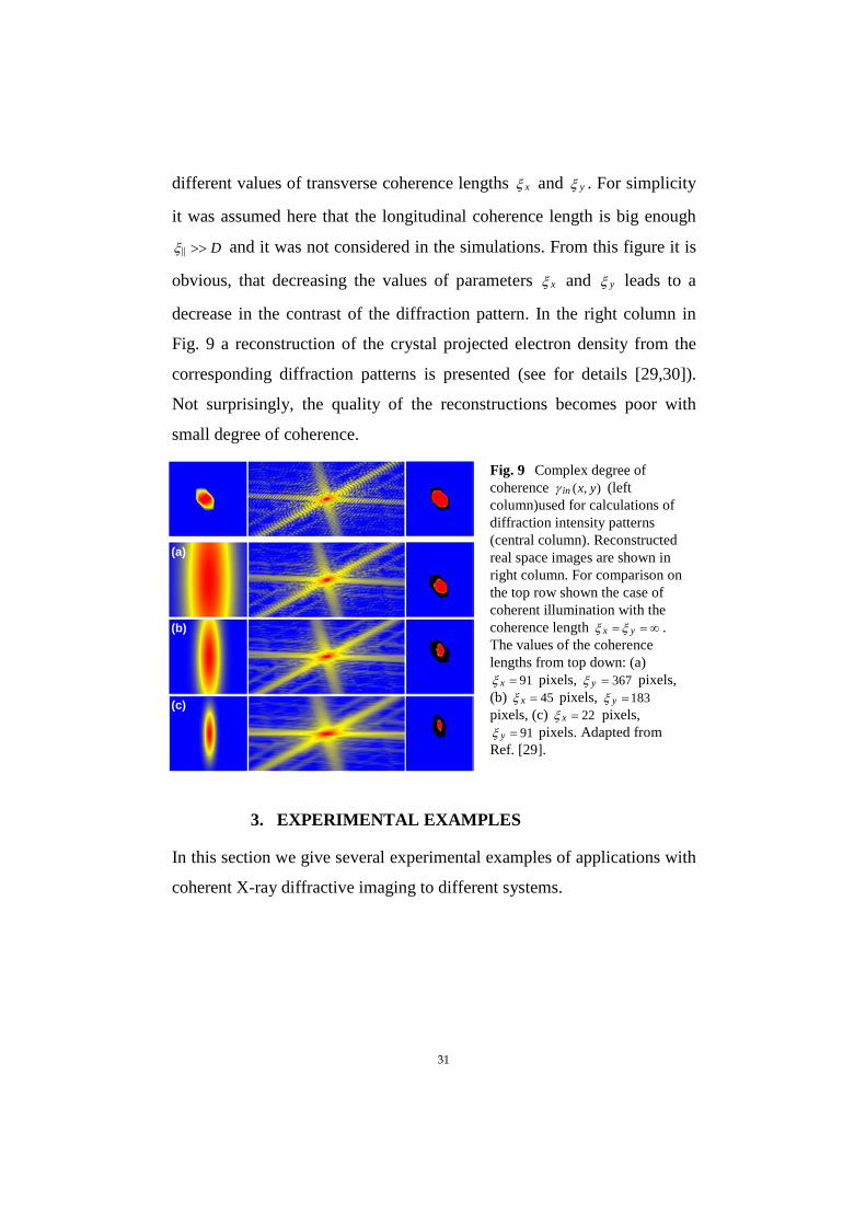
In Fig. 9 we present calculations of 2D diffraction patterns obtained

from Eq. (52) for the crystal shape shown in the left inset of Fig. 5 with

31

different values of transverse coherence lengths xξ and yξ . For simplicity

it was assumed here that the longitudinal coherence length is big enough

D>>||ξ and it was not considered in the simulations. From this figure it is

obvious, that decreasing the values of parameters xξ and yξ leads to a

decrease in the contrast of the diffraction pattern. In the right column in

Fig. 9 a reconstruction of the crystal projected electron density from the

corresponding diffraction patterns is presented (see for details [29,30]).

Not surprisingly, the quality of the reconstructions becomes poor with

small degree of coherence.

3. EXPERIMENTAL EXAMPLES

In this section we give several experimental examples of applications with

coherent X-ray diffractive imaging to different systems.

(a)

(b)

(c)

Fig. 9 Complex degree of coherence ),( yxinγ (left column)used for calculations of diffraction intensity patterns (central column). Reconstructed real space images are shown in right column. For comparison on the top row shown the case of coherent illumination with the coherence length ∞== yx ξξ . The values of the coherence lengths from top down: (a)

91=xξ pixels, 367=yξ pixels, (b) 45=xξ pixels, 183=yξ pixels, (c) 22=xξ pixels,

91=yξ pixels. Adapted from Ref. [29].

32

3.1 Coherent X-ray imaging of defects in colloidal crystals

First, we present results of CXDI applied to reveal the structure of a

regular part and also a part containing a defect of a colloidal 2D crystal

(see for details [53]).

Self-organized colloidal crystals are an attractive material for modern

technological devices. They can be used as the basis for novel functional

materials such as photonic crystals, which may find applications in future

solar cells, LEDs, lasers or even as the basis for circuits in optical

computing and communication. For these applications the crystal quality

is crucial and monitoring the defect structure of real colloidal crystals is

essential [72].

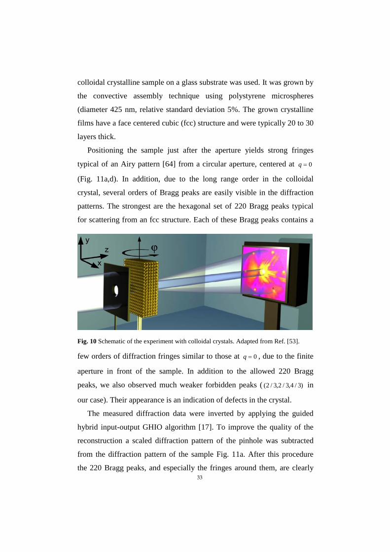
The experiment [53] was performed at the microoptics test bench at the

ID06 beamline of the European Synchrotron Radiation Facility (ESRF)

using an incident X-ray energy of 14 keV. The geometry of the

experiment allows for rotation of the sample around the vertical axis

which is perpendicular to the incident X-ray direction (see sketch Fig. 10).

A 6.9 µm pinhole was positioned at a close distance in front of the

colloidal crystal. The pinhole selects a highly coherent part of the beam

and produces a finite illumination area. The initial orientation of the

sample (with azimuthal angle 0=ϕ ) corresponds to the direction of the

incident X-rays along the [111] direction of the fcc colloidal crystal and

was perpendicular to the surface normal of the sample. Rotating the

sample around the x -axis allows the measurement of different sets of

diffraction planes. Particularly important was the direction of the incident

X-rays along the [110] direction of the colloidal sample lattice at 35=ϕ ,

when the set of (111) planes was aligned along the incident beam. The

diffraction data were recorded using a CCD with 4005×2671 pixels with a

resolution of 16.0=∆q µm 1− per pixel. In experiment a thin film of a

33

colloidal crystalline sample on a glass substrate was used. It was grown by

the convective assembly technique using polystyrene microspheres

(diameter 425 nm, relative standard deviation 5%. The grown crystalline

films have a face centered cubic (fcc) structure and were typically 20 to 30

layers thick.

Positioning the sample just after the aperture yields strong fringes

typical of an Airy pattern [64] from a circular aperture, centered at 0=q

(Fig. 11a,d). In addition, due to the long range order in the colloidal

crystal, several orders of Bragg peaks are easily visible in the diffraction

patterns. The strongest are the hexagonal set of 220 Bragg peaks typical

for scattering from an fcc structure. Each of these Bragg peaks contains a

few orders of diffraction fringes similar to those at 0=q , due to the finite

aperture in front of the sample. In addition to the allowed 220 Bragg

peaks, we also observed much weaker forbidden peaks ( )3/4,3/2,3/2( in

our case). Their appearance is an indication of defects in the crystal.

The measured diffraction data were inverted by applying the guided

hybrid input-output GHIO algorithm [17]. To improve the quality of the

reconstruction a scaled diffraction pattern of the pinhole was subtracted

from the diffraction pattern of the sample Fig. 11a. After this procedure

the 220 Bragg peaks, and especially the fringes around them, are clearly

Fig. 10 Schematic of the experiment with colloidal crystals. Adapted from Ref. [53].

34

visible against the background Fig. 11b. Negative values, shown in black

in the difference diffraction pattern in Fig. 11b, were left to evolve freely

in the reconstruction procedure. To stabilize the reconstruction process the

central region (with 44.5<q µm 1− ) of the reconstructed diffraction pattern

was kept fixed after 20 initial iterations.

A real space image of a colloidal sample obtained as a result of

reconstruction of the diffraction pattern shown in Fig. 11b is presented in

Fig. 11c. This image represents a projection of the 'atomic' structure of the

colloidal crystal along the [111] direction. The hexagonal structure is clear

across the whole illuminated region, with only slightly lower intensity

values of the image around the edges of the pinhole aperture. As a

consequence of the image being a projection of 3D arrangement of

colloidal particles, the periodicity does not correspond to the colloidal

interparticle distance d in a single crystalline layer. Due to ABC ordering

in fcc crystals a reduced periodicity of 3/d is measured in this geometry.

The major differences from the results of previous work with CXDI on

crystalline samples [44] are clearly demonstrated in Fig. 11c. Instead of a

continuous shape and strain field reconstructed from the measurements of

diffraction patterns around a single Bragg peak, the hexagonal structure

shown in Fig. 11c gives the projected positions of the colloidal particles as

it was discussed in details in section 2.1

35

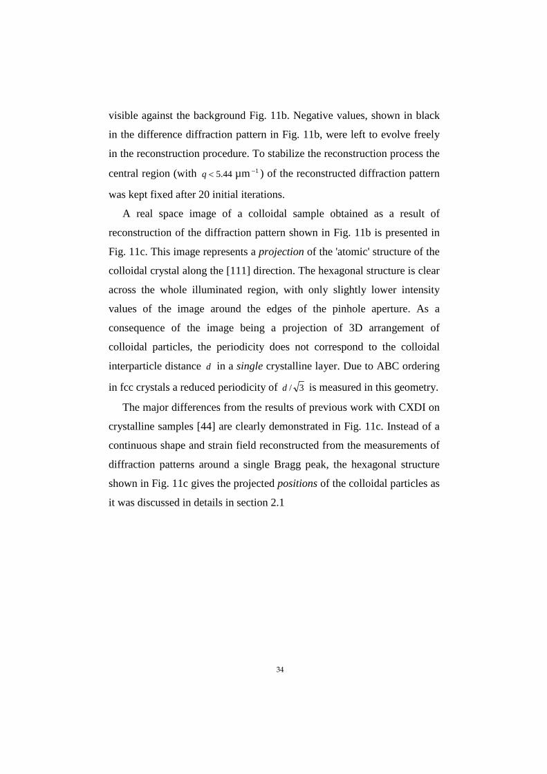
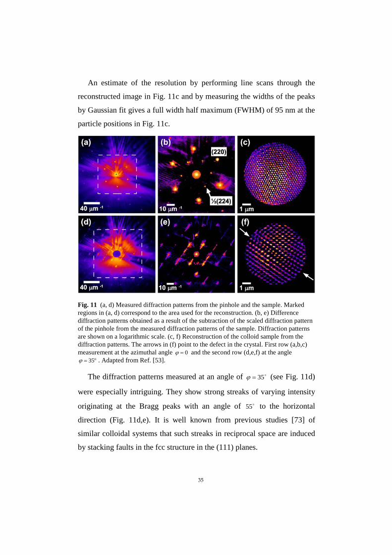
An estimate of the resolution by performing line scans through the

reconstructed image in Fig. 11c and by measuring the widths of the peaks

by Gaussian fit gives a full width half maximum (FWHM) of 95 nm at the

particle positions in Fig. 11c.

The diffraction patterns measured at an angle of 35=ϕ (see Fig. 11d)

were especially intriguing. They show strong streaks of varying intensity

originating at the Bragg peaks with an angle of 55 to the horizontal

direction (Fig. 11d,e). It is well known from previous studies [73] of

similar colloidal systems that such streaks in reciprocal space are induced

by stacking faults in the fcc structure in the (111) planes.

Fig. 11 (a, d) Measured diffraction patterns from the pinhole and the sample. Marked regions in (a, d) correspond to the area used for the reconstruction. (b, e) Difference diffraction patterns obtained as a result of the subtraction of the scaled diffraction pattern of the pinhole from the measured diffraction patterns of the sample. Diffraction patterns are shown on a logarithmic scale. (c, f) Reconstruction of the colloid sample from the diffraction patterns. The arrows in (f) point to the defect in the crystal. First row (a,b,c) measurement at the azimuthal angle 0=ϕ and the second row (d,e,f) at the angle

°= 35ϕ . Adapted from Ref. [53].

36

These diffraction patterns were reconstructed using the same procedure

as described earlier and the result of this reconstruction is presented in Fig.

11f. The 'atomicity' of the colloidal crystal sample is again present in the

reconstruction. In addition, a stacking fault appears (indicated by arrows in

Fig. 11f) as a break in the 'correct' ABC ordering [33]. One can see a

stacking fault, which consists of two hcp planes, and two fcc domains with

the same stacking direction. The effect of the stacking fault is a translation

of the two fcc crystals relative to each other. This 'sliding' can be seen in

Fig. 11f as a 'break' of the lines of bright spots at the defect. It was

recently suggested that, over a large (submillimeter) sample area, these

double stacking defects consisting of two hcp planes is a common

imperfection in convectively assembled colloidal crystals [74].

In this part we demonstrated that the simple and nondestructive

mechanism of coherent X-ray diffractive imaging opens a unique route to

determine the structure of mesoscopic materials such as colloidal crystals.

CXDI has the potential to provide detailed information about the local

defect structure in colloidal crystals. This is especially important for

imaging photonic materials when refraction index matching is not possible

or the sizes of colloidal particles are too small for conventional optical

microscopy. To extend this method to larger fields of view scanning

methods such as ptychography [18-20] can be used, while tomographic

methods such as coherent X-ray tomography [75] have the potential to

visualize the atomic structure of the defect core in 3D (see, for example,

recent publication [54]).

37

3.2 Coherent diffraction tomography of nanoislands from

grazing incidence small-angle X-ray scattering

In our second example we show how tomographic methods can be

combined with CXDI to provide 3D images of nanocrystaline materials

(see for details [75]).

Tomography and especially X-ray tomography has become one of the

most important tools for investigating 3D structures in condensed matter

[76]. When projected absorption contrast or phase contrast measurements

are carried out in conventional X-ray transmission tomography the

achievable resolution is limited by the spatial resolution of the area

detector that can be about one micrometer. CXDI represents a possible

solution to this dilemma. As no lenses are required in this imaging

technique and the resolution is given by the scattered signal in principle

the resolution limits of conventional X-ray transmission tomography can

be overcome.

To obtain a 3D image of a non-crystallographic object in the forward

scattering geometry by the CXDI technique the sample is usually mounted

on a 43NSi membrane (see for e.g. [77]) and then rotated with fixed

azimuthal angular steps (see inset (a) in Fig. 12). Unfortunately, in this

approach not all angles for a full 3D scan are accessible due to the

positioning of the object on a membrane. Obviously, the inaccessible part

of the reciprocal space is not available for the tomographic reconstruction,

resulting in a certain loss of features which are actually present in the

original object. Instead, as it was first proposed in [48,75], a sample can be

positioned on a flat thick substrate and tomographic scans can be

performed by collecting successive coherent scattering diffraction patterns

at different azimuthal positions of a sample in a grazing-incidence small-

angle X-ray scattering (GISAXS) geometry [48] (see Fig. 12). With this

approach there are no limitations on the angle of rotation. Consequently

38

large areas in reciprocal space can be measured with sufficient resolution

and without missing wedge. The feasibility of this approach was tested

and proven by a number of simulations [78]. Below experimental

realization of this coherent diffraction tomographic technique is reported [75].

As a model samples SiGe islands of 200 nm average base size grown

by liquid phase epitaxy were used. All islands were coherently grown on a

(001) Si surface and exhibit a truncated pyramidal shape with a square

base (see inset (b) in Fig. 12). In addition they exhibit a narrow size

distribution (~10% full width at half maximum (FWHM)) and the same

crystallographic orientation on the Si surface (Fig. 12).

Experiments [48,75,79] were performed at the ID01 beamline of the

European Synchrotron Radiation Facility (ESRF) in Grenoble. The

incidence angle was taken equal to the critical angle for total external

reflection of the Si substrate which corresponds to 224.0== ci αα for the

chosen X-ray energy of 8 keV. This particular angle was used because at

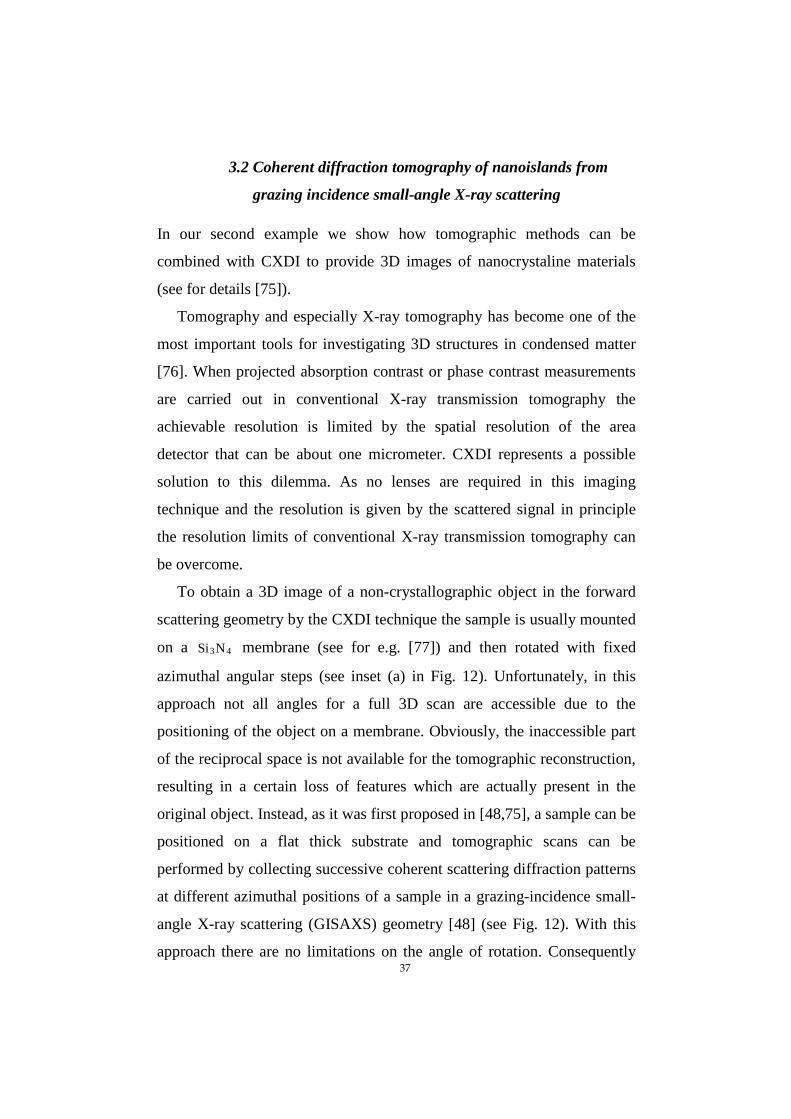
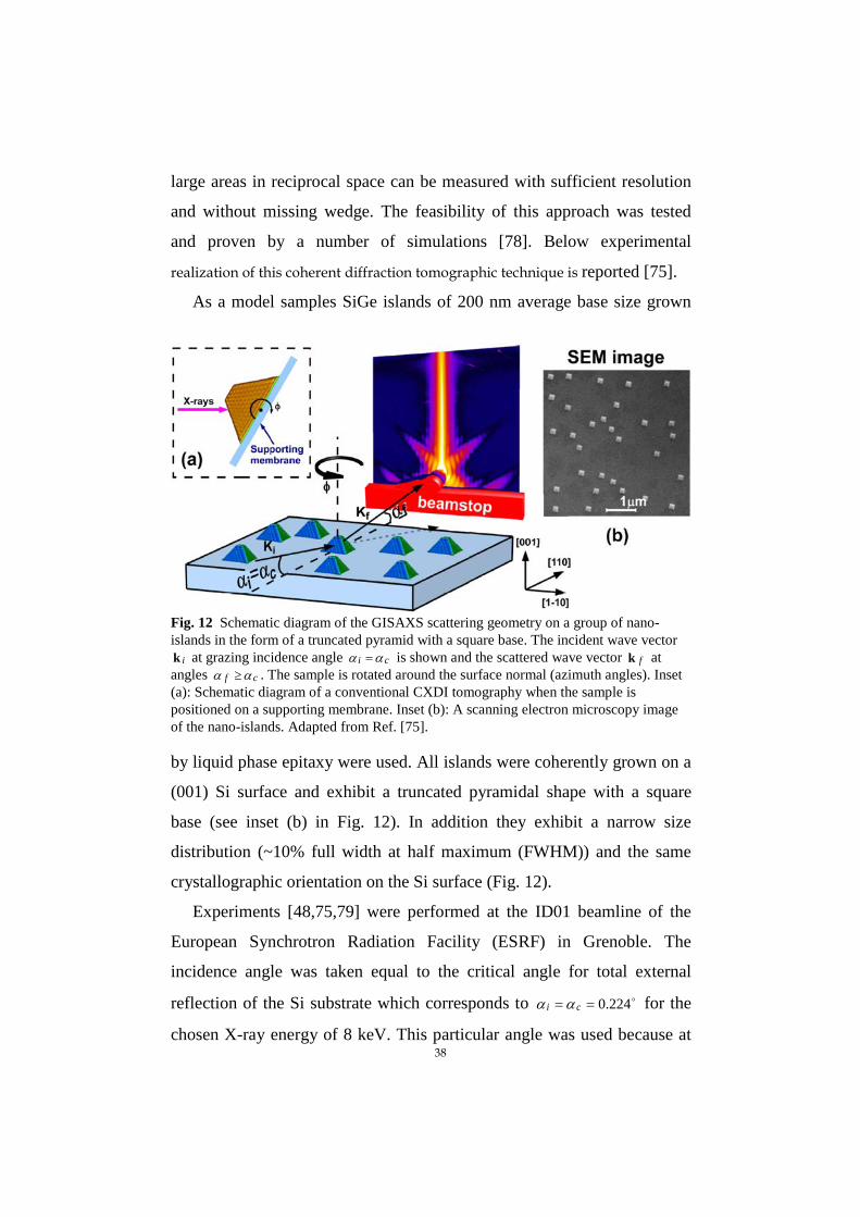
Fig. 12 Schematic diagram of the GISAXS scattering geometry on a group of nano-islands in the form of a truncated pyramid with a square base. The incident wave vector

ik at grazing incidence angle ci αα = is shown and the scattered wave vector fk at angles cf αα ≥ . The sample is rotated around the surface normal (azimuth angles). Inset (a): Schematic diagram of a conventional CXDI tomography when the sample is positioned on a supporting membrane. Inset (b): A scanning electron microscopy image of the nano-islands. Adapted from Ref. [75].

39

these conditions the scattering may be considered as predominantly

kinematical [80]. The coherently scattered signal was measured up to

56.0|| ±=q nm 1− in reciprocal space in the transverse direction. However,

due to a certain noise level only a limited part of reciprocal space up to

36.0|| ±=q nm 1− was considered for the reconstruction, which provides a

17.4 nm resolution in real space. An azimuth scan was performed from 5°

to 50° with an angular increment of 1°. Due to the four fold and mirror

symmetry of {111} facetted islands such scans cover the whole reciprocal

space. During the azimuthal scan the incidence angle was kept constant at

the critical angle cα .

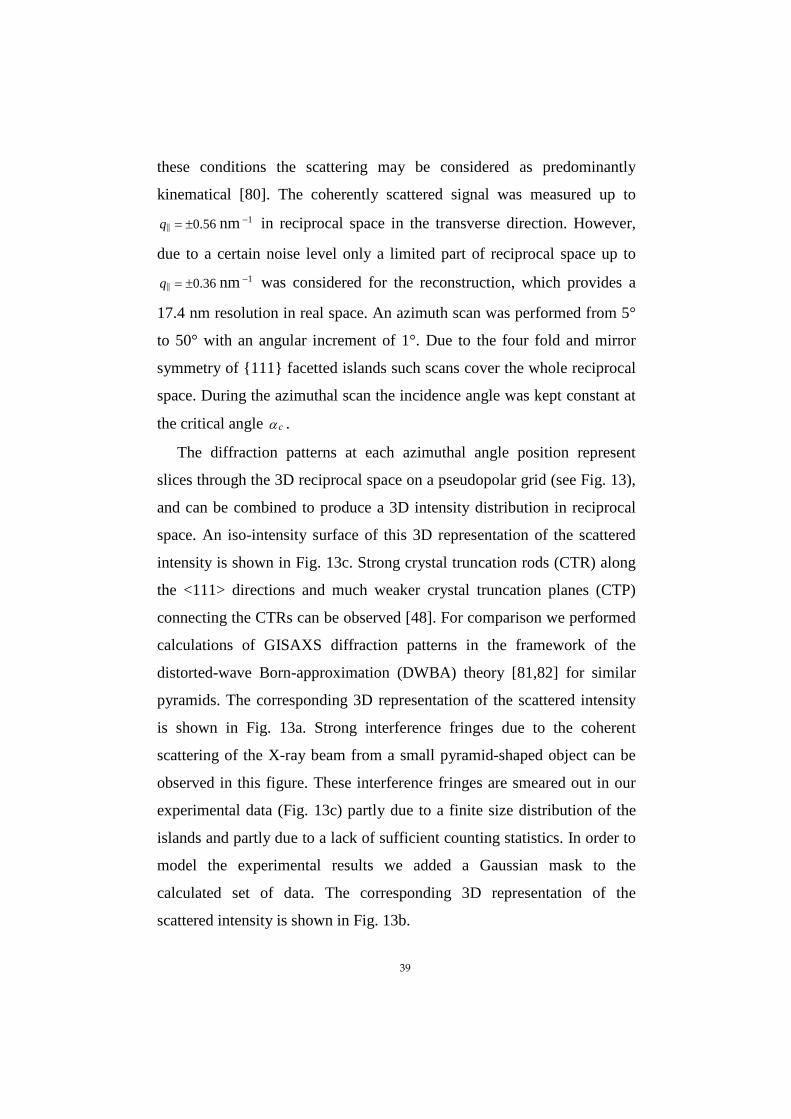
The diffraction patterns at each azimuthal angle position represent

slices through the 3D reciprocal space on a pseudopolar grid (see Fig. 13),

and can be combined to produce a 3D intensity distribution in reciprocal

space. An iso-intensity surface of this 3D representation of the scattered

intensity is shown in Fig. 13c. Strong crystal truncation rods (CTR) along

the <111> directions and much weaker crystal truncation planes (CTP)

connecting the CTRs can be observed [48]. For comparison we performed

calculations of GISAXS diffraction patterns in the framework of the

distorted-wave Born-approximation (DWBA) theory [81,82] for similar

pyramids. The corresponding 3D representation of the scattered intensity

is shown in Fig. 13a. Strong interference fringes due to the coherent

scattering of the X-ray beam from a small pyramid-shaped object can be

observed in this figure. These interference fringes are smeared out in our

experimental data (Fig. 13c) partly due to a finite size distribution of the

islands and partly due to a lack of sufficient counting statistics. In order to

model the experimental results we added a Gaussian mask to the

calculated set of data. The corresponding 3D representation of the

scattered intensity is shown in Fig. 13b.

40

Results of the island shape reconstruction from the experimental

GISAXS diffraction patterns are presented in Fig. 13f. For a comparison

results of the reconstruction of the island shape from simulated data are

also shown in Fig. 13d,e. The electron densities of the islands obtained as

a vertical section through the center of the islands are presented in Fig.

13g-i. From these results it is seen that the shape of the islands is

Fig. 13 Left column [(a), (d), (g)]: simulations in the framework of the DWBA theory. Middle column [(b), (e), (h)]: simulations in the framework of the DWBA theory with an additional Gaussian mask (see text for details). Right column [(c), (f), (i)]: experiment. [(a), (b),(c)]: 3D plot of an iso-intensity surface in the reciprocal space. RGB colors correspond to the z-projection of the iso-surface normal. Grey arrows indicate directions along the crystallographic planes (001) top and {111} on the side. Black arrows indicate

zyx qqq ,, directions in reciprocal space. The length of each black arrow corresponds to 0.1 nm-1. [(d), (e), (f)]: Reconstructed shape of the islands. The transparent box indicates the size of the support. [(g), (h), (i)]: Electron density of the islands obtained as a vertical section through the center of each island. Adapted from Ref. [75].

41

reconstructed correctly for the experimental data set (Fig. 13f). However,

for the electron density inside the island we observe artifacts in the form

of low density regions in the bottom of the islands (Fig. 13i).

Reconstructions performed with the simulated data sets show that the

scattering data obtained in the DWBA conditions correctly reproduce the

shape (Fig. 13d) and electron density (Fig. 13g) of an island. However,

when the modified theoretical data set with the Gaussian mask is used for

reconstruction, artifacts similar to those from the experimental data set

appear. These results suggest that the artifacts can be removed by an

increased incidence flux (e.g. by using focusing optics [22]) and with the

use of a new generation of detectors with extremely high dynamic range.

Here we have demonstrated how this approach of coherent diffraction

GISAXS can be used to obtain the 3D electron density of nanometer sized

islands. This was achieved by performing tomographic azimuth scans in a

GISAXS geometry on many identical islands and subsequent phase

retrieval which yields the tomographic information, such as the shape and

the electron density. It is important to note that this approach does not

depend on the crystalline structure of such an island and may be applied to

any material system.

3.3 Coherent-pulse 2D crystallography at free electron lasers

As our third example we show how ultra-bright coherent pulses of a new

free-electron laser (FEL) sources can be applied to determine the structure

of two-dimensional (2D) crystallographic objects (see for details Ref. [83],

and also for reviews of CXDI experiments at FEL source [5,6,9]).

Crystallization and radiation damage is presently a bottleneck in

protein structure determination. As it was first proposed in Ref. [83] two-

dimensional (2D) finite crystals and ultra-short FEL pulses can be

effectively used to reveal the structure of single molecules. This can be

42

especially important for membrane proteins that in general do not form 3D

crystals, but easily form 2D crystalline structures. In this paper single

pulse train coherent diffractive imaging was demonstrated for a finite 2D

crystalline sample, and it was concluded that this alternative approach to

single molecule imaging is a significant step towards revealing the

structure of proteins with sub-nanometer resolution at the newly built

XFEL sources.

Revealing the structure of protein molecules is mandatory for

understanding the structure of larger biological complexes. The major

progress in uncovering the structure of proteins in past decades was due to

the development of phasing methods [84] allowing the determination of

the structure of complex molecules that crystallize. One new approach to

overcome these difficulties is based on the use of ultra-short pulses of X-

ray free-electron lasers (XFEL) [85-87]. This elegant idea is based on

measuring a sufficiently sampled diffraction pattern from a single

molecule illuminated by an FEL pulse [88,89]. However, in spite of the

extreme intensity of the FEL pulses, a diffraction pattern from only one

molecule will not be sufficient to obtain a high resolution diffraction

pattern. Many reproducible copies will need to be measured to get a

sufficient signal to noise ratio for each projection necessary for three-

dimensional (3D) imaging at sub-nanometer spatial resolution.

Free-electron lasers are especially well suited for such coherent 2D

crystallography. They provide femtosecond coherent pulses [70,90,91]

with extremely high power. Only the combination of all of these unique

properties will allow the realization of 2D crystallographic X-ray imaging

on biological systems. Brilliant, ultra-short pulses could overcome the

radiation damage problem [88,92] which is a severe limitation of

conventional crystallography at 3rd generation synchrotron sources [93].

Higher luminosity and hence improved statistics for such experiments can

43

be obtained by the use of pulse trains that can be provided by FLASH

(Free-electron LASer in Hamburg) [94].

A finite 2D crystallography was demonstrated by using a micro-

structured crystal array that was prepared on a 100 nm thick silicon nitride

membrane substrate coated with 600 nm of gold, and 200 nm of

palladium. The finite crystal sample was manufactured by milling holes in

the film in a regular array pattern using a Focused Ion Beam (FIB). The

'unit cell' of our crystal consists of a large hole of 500 nm diameter

(representing a 'heavy atom' in conventional crystallography) and a

smaller hole of 200 nm diameter (representing a 'light atom'). The whole

structure was composed of five unit cells in each direction, making the

total structure size about 10 µm x 10 µm.

The diffraction data were measured at FLASH on the PG2

monochromator beamline [95] with a fundamental wavelength of 7.97 nm.

An exposure time of 0.2 s was used to collect a series of single pulse train

data from our sample. FLASH was operated in a regime producing 21

bunches of electrons per pulse train, with a pulse train repetition rate of 5

Hz. The bunches within each pulse train were spaced at 1 MHz. The

average pulse energy was 15 μJ which is equivalent to 11106× photons per

pulse or 13103.1 × photons per train at the source. The coherent flux on the

sample area was 10105.1 × photons per pulse train.

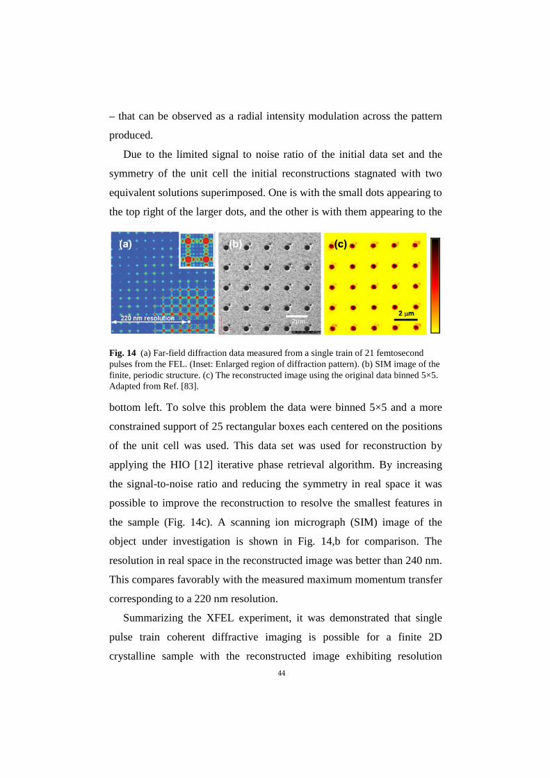
A typical data set is shown in Fig. 14a. The diffraction pattern as

measured fills the whole detector, which corresponds to a minimum

feature size of 220 nm (Fig. 14a). We note that all expected features of a

finite, crystalline structure as they were discussed in the previous sections

are observed in this diffraction pattern. The Bragg peaks due to the regular

array are clearly seen, as are the oscillations between the Bragg peaks that

are the result of the finite extent and coherent illumination of our sample.

Also seen is the form factor from the individual elements – the large holes

44

– that can be observed as a radial intensity modulation across the pattern

produced.

Due to the limited signal to noise ratio of the initial data set and the

symmetry of the unit cell the initial reconstructions stagnated with two

equivalent solutions superimposed. One is with the small dots appearing to

the top right of the larger dots, and the other is with them appearing to the

bottom left. To solve this problem the data were binned 5×5 and a more

constrained support of 25 rectangular boxes each centered on the positions

of the unit cell was used. This data set was used for reconstruction by

applying the HIO [12] iterative phase retrieval algorithm. By increasing

the signal-to-noise ratio and reducing the symmetry in real space it was

possible to improve the reconstruction to resolve the smallest features in

the sample (Fig. 14c). A scanning ion micrograph (SIM) image of the

object under investigation is shown in Fig. 14,b for comparison. The

resolution in real space in the reconstructed image was better than 240 nm.

This compares favorably with the measured maximum momentum transfer

corresponding to a 220 nm resolution.

Summarizing the XFEL experiment, it was demonstrated that single

pulse train coherent diffractive imaging is possible for a finite 2D

crystalline sample with the reconstructed image exhibiting resolution

Fig. 14 (a) Far-field diffraction data measured from a single train of 21 femtosecond pulses from the FEL. (Inset: Enlarged region of diffraction pattern). (b) SIM image of the finite, periodic structure. (c) The reconstructed image using the original data binned 5×5. Adapted from Ref. [83].

45

commensurate with the measured data. In this experiment the crystalline

structure was essential in providing the necessary information to

determine the structure of the unit cells. If only a single unit cell would

have been used simulations suggest that a successful reconstruction would

be impossible with the resolution presented in the example. This approach

to use a pattern of single molecules is a significant step towards revealing

the structure of proteins with sub-nanometer resolution at the newly built

XFEL sources.

4. SUMMARY

Coherent X-ray diffractive imaging gives us a high resolution imaging tool

to reveal the electron density and strain in nano-crystalline samples.

Progress is still ongoing. We foresee that in future it will reach a

resolution of approximately a few nanometers at synchrotron sources, and

a few angstroms for the protein nano-crystals imaged with the ultrashort

FEL pulses [96]. Non-reproducible objects may be imaged with a few

nanometer resolution at XFELs [9,26,97]. There are several technological

developments that are incremental for the future progress of the CXDI

technique. The ultimate hard X-ray storage rings [98] with a few tens

picometer emittance are under discussion. The advances in hard X-ray

optics will allow reaching sub-ten nanometer focus sizes [99]. Also, hard

X-ray FEL sources now become online. Finally, the mathematical tools for

interpretation of data from coherent X-ray scattering experiments improve

continuously. Thus, we can expect that CXDI will become eminently

important for the investigation of the structure of materials on the

nanoscale and will grow rapidly over the near future.

The authors acknowledge a careful reading of the manuscript by O. Seeck and B. Murphy.

46

References 1. Vartanyants, I. A., Pitney, J. A., Libbert, J. L. and Robinson, I. K. (1997). Reconstruction of

Surface Morphology from Coherent X-ray Reflectivity. Phys. Rev. B, 55, pp. 13193-13202. 2. Miao, J., Charalambous, P., Kirz, J. and Sayre, D. (1999). Extending the methodology of X-

ray crystallography to allow imaging of micrometre-sized non-crystalline specimens. Nature, 400, pp. 342-344.

3. Robinson, I. K., Libbert, J. L., Vartanyants, I. A., Pitney, J. A., Smilgies, D. M., Abernathy, D. L., and Grübel, G. (1999). Coherent X-ray Diffraction Imaging of Silicon Oxide Growth. Phys. Rev. B, 60, pp. 9965-9972.

4. Robinson, I. K., Vartanyants, I. A., Williams, G. J., Pfeifer, M. A. and Pitney, J. A. (2001). Reconstruction of the Shapes of Gold Nanocrystals using Coherent X-ray Diffraction. Phys. Rev. Lett., 87, pp. 195505.

5. Vartanyants, I. A., Robinson, I. K., McNulty, I., David, C., Wochner, P. and Tschentscher, Th. (2007). Coherent X-ray scattering and lensless imaging at the European XFEL Facility. J. Synchrotron Rad., 14, pp. 453-470.

6. Vartanyants, I. A., Mancuso, A. P., Singer, A., Yefanov, O. M. and Gulden, J. (2010). Coherence Measurements and Coherent Diffractive Imaging at FLASH. J. Phys. B: At. Mol. Opt. Phys., 43, pp. 194016/1-10.

7. Nugent, K.A. (2010). Coherent methods in the X-ray sciences. Advances in Physics 59, 1-99. 8. Robinson, I. K. and Harder, R. (2009). Coherent X-ray diffraction imaging of strain at the

nanoscale. Nature Mater., 8, pp. 291-298. 9. Mancuso, A. P., Yefanov, O. M. and Vartanyants, I. A. (2010). Coherent diffractive imaging

of biological samples at synchrotron and free electron laser facilities. J. Biotechnol., 149, pp. 229-237.

10. Quiney, H. M. (2011). Coherent diffractive imaging using short wavelength light sources. J. Mod. Opt., 57, pp. 1109-1149.

11. Gerchberg, R. W. and Saxton, W. O. (1972). A Practical Algorithm for the Determination of Phase from Image and Diffraction Plane Pictures. Optik, 35, pp. 237-246.

12. Fienup, J. R. (1982). Phase retrieval algorithms: a comparison. Appl. Opt., 21, pp. 2758-2769. 13. Elser, V. (2003). Phase retrieval by iterated projections. J. Opt. Soc. Am. A, 20, pp. 40-55. 14. Marchesini, S. (2007). A unified evaluation of iterative projection algorithms for phase

retrieval. Rev. Sci. Instr., 78, pp. 049901. 15. Bates, R. H. T. (1982). Fourier phase problems are uniquely solvable in more than one

dimension. I: Underlying theory. Optik, 61, pp. 247-262. 16. Shannon, C. E. (1949). Communication in the Presence of Noise. Proc. IRE, 37, pp. 10-21. 17. Chen, C.-C., Miao, J., Wang, C. W. and Lee, T. K. (2007). Application of optimization

technique to noncrystalline X-ray diffraction microscopy: Guided hybrid input-output method. Phys. Rev. B, 76, pp. 064113.

18. Rodenburg, J. M., Hurst, A. C., Cullis, A. G., Dobson, B. R., Pfeiffer, F., Bunk, O., David, C., Jefimovs, K. and Johnson, I. (2007). Hard-X-Ray Lensless Imaging of Extended Objects. Phys. Rev. Lett., 98, pp. 034801.

19. Thibault, P., Dierolf, M., Menzel, A., Bunk, O., David, Ch. and Pfeiffer, F. (2008). High-Resolution Scanning X-ray Diffraction Microscopy. Science, 321, pp. 379-382.

20. Schropp, A., Boye, P., Feldkamp, J. M., Hoppe, R., Patommel, J., Samberg, D., Stephan, S., Giewekemeyer, K., Wilke, R. N., Salditt, T., Gulden, J., Mancuso, A. P., Vartanyants, I. A., Weckert, E., Schöder, S., Burghammer, M., and Schroer C. G. (2010). Hard x-ray nanobeam characterization by coherent diffraction microscopy. Appl. Phys. Lett., 96, pp. 091102/1-3.

47

21. Godard, P., Carbone , G., Allain, M., Mastropietro, F., Chen , G., Capello , L., Diaz, A., Metzger, T. H., Stangl J. and Chamard, V. (2011). Three-dimensional high-resolution quantitative microscopy of extended crystals. Nature Comm., 2, pp. 568.

22. Takahashi, Y., Zettsu, N., Nishino, Y., Tsutsumi, R., Matsubara, E., Ishikawa, T. and Yamauchi, K. (2010). Three-Dimensional Electron Density Mapping of Shape-Controlled Nanoparticle by Focused Hard X-ray Diffraction Microscopy. Nano Lett., 10, pp. 1922-1926.

23. Giewekemeyer, K ., Pierre Thibault, P., Kalbfleisch, S., Beerlink, A., Kewish, C. M., Dierolf, M., Pfeiffer, F. and Salditt T. (2010). Quantitative biological imaging by ptychographic X-ray diffraction microscopy. Proc. Natl. Acad. Sci. USA, 107, pp. 529-534.

24. Dierolf, M., Menzel, A., Thibault, P., Schneider, P., Kewish, C. M., Wepf, R., Bunk O. and Pfeiffer F. (2010). Ptychographic X-ray computed tomography at the nanoscale. Nature, 467, pp. 436-439.

25. Shen, Q., Bazarov, I. and Thibault, P. (2004). Diffractive imaging of nonperiodic materials with future coherent X-ray sources. J. Synchrotron Rad., 11, pp. 432-438.

26. Bergh, M., Huldt, G., Timneanu, N., Maia, F. R. N. C. and Hajdu, J. (2008). Feasibility of imaging living cells at subnanometer resolutions by ultrafast X-ray diffraction. Q. Rev. Biophys., 41, pp. 181-204.

27. Huang, X., Miao, H., Steinbrener, J., Nelson, J., Shapiro, D., Stewart, A., Turner, J. and Jacobsen, Ch. (2009). Signal-to-noise and radiation exposure considerations in conventional and diffraction microscopy. Optics Express, 17, pp. 13541-13553.

28. Thibault, P., Elser, V., Jacobsen, C., Shapiro D. and Sayre D. (2006). Reconstruction of a yeast cell from X-ray diffraction data. Acta Cryst. A, 62, pp. 248-261.

29. Vartanyants, I. A. and Robinson. I. K. (2001). Partial coherence effects on the imaging of small crystals using coherent X-ray diffraction. J. Phys.: Condens. Matter, 13, pp. 10593-10611.

30. Vartanyants, I. A. and Robinson, I. K. (2003). Origins of decoherence in coherent X-ray diffraction experiments. Opt. Commun., 222, pp. 29-50.

31. Williams, G. J., Quiney, H. M., Peele, A. G. and Nugent, K. A. (2007). Coherent diffractive imaging and partial coherence. Phys. Rev. B, 75, pp. 104102.

32. Millane, R. P. (1990). Phase retrieval in crystallography and optics. J. Opt. Soc. Am. A, 7, pp. 394-411.

33. Warren, B. E. (1990). X-ray Diffraction. (Dover Publ. Inc., New York). 34. Als-Nielsen, J. and McMorrow, D. (2011). Elements of modern X-ray physics. (John Wiley

and Sons, New York). 35. Batterman, B. W., and Cole H. (1964). Dynamical Diffraction of X Rays by Perfect Crystals.

Rev. Mod. Phys., 36, pp. 681-717. 36. Authier A. (2003). Dynamical theory of X-ray diffraction. (Oxford University Press, 2-nd

edition, Oxford). 37. Shabalin, A., Yefanov, O. M., Nosik, V. L. and Vartanyants, I. A. Dynamical effects in

coherent X-ray scattering on a finite crystal. (In preparation). 38. Harder, R., Pfeifer, M. A., Williams, G. J., Vartanyants, I. A. and Robinson, I. K. (2007).

Orientation variation of surface strain. Phys. Rev. B, 76, pp. 115425/1-4. 39. Ewald, P. P. (1940). X-ray diffraction by finite and imperfect crystal lattices. Proc. Phys. Soc.,

52, pp. 167. 40. von Laue, M. (1936). Die äußere Form der Kristalle in ihrem Einfluß auf die

Interferenzerscheinungen an Raumgittern. Ann. d. Physik, 26, pp. 55. 41. Sayre, D. (1952). Some implications of a theorem due to Shannon. Acta Cryst., 5, pp. 843. 42. Williams, G. J., Pfeifer, M. A., Vartanyants, I. A. and Robinson, I. K. (2003). Three-

Dimensional Imaging of Microstructure in Au Nanocrystals. Phys. Rev. Lett., 90, pp. 175501. 43. Millane, R. P. (1996). Multidimensional phase problems. J. Opt. Soc. Am. A, 13, pp. 725.

48

44. Pfeifer, M. A., Williams, G. J., Vartanyants, I. A., Harder, R. and Robinson, I. K. (2006). Three-dimensional mapping of a deformation field inside a nanocrystal. Nature, 442, pp, 63-66.

45. Robinson, I. K. (1986). Crystal truncation rods and surface roughness. Phys. Rev. B, 33, pp. 3830-3836.

46. Afanas’ev, A. M., Aleksandrov, P. A., Imamov, R. M., Lomov, A. A. and Zavyalova, A. A. (1985). Three-Crystal Diffractometry in Grazing Bragg-Laue Geometry. Acta Cryst. A, 41, pp. 227.

47. Pitney, J. A., Robinson, I. K., Vartanyants, I. A., Appelton, R. and Flynn, C. P. (2000).Streaked speckle in Cu3Au coherent diffraction. Phys. Rev. B 62, 13084-13088.

48. Vartanyants, I. A., Zozulya, A. V., Mundboth, K., Yefanov, O. M., Richard, M.-I., Wintersberger, E., Stangl, J., Diaz, A., Mocuta, C., Metzger, T. H., Bauer, G., Boeck, T. and Schmidbauer, M. (2008). Crystal truncation planes revealed by three-dimensional reconstruction of reciprocal space. Phys. Rev. B 77, 115317.

49. Eisebitt, S., Luning, J., Schlotter, W. F., Lorgen, M., Hellwig, O., Eberhardt, W. and Stohr, J. (2004). Lensless imaging of magnetic nanostructures by X-ray spectro-holography. Nature 432, 885-888.

50. Stadler, L.-M., Gutt, Ch., Autenrieth, T., Leupold, O., Rehbein, S., Chushkin, Y. and Grübel, G. (2008). Hard X-Ray Holographic Diffraction Imaging. Phys. Rev. Lett. 100, 245503.

51. Chamard, V., Stangl, J., Carbone, G., Diaz, A., Chen, G., Alfonso, C., Mocuta, C. and Metzger, T. H. (2010), Three-Dimensional X-Ray Fourier Transform Holography: The Bragg Case. Phys. Rev. Lett. 104, 165501.

52. Gulden, J., Yefanov, O. M., Weckert, E., and Vartanyants, I.A. (2011). Imaging of Nanocrystals with Atomic Resolution Using High-Energy Coherent X-rays. The 10th International Conference on X-ray Microscopy, AIP Conf. Proc. 1365, 42-45.

53. Gulden, J., Yefanov, O. M., Mancuso, A. P., Abramova, V. V., Hilhorst, J., Byelov, D., Snigireva, I., Snigirev, A., Petukhov, A. V. and Vartanyants, I. A. (2010). Coherent X-ray imaging of defects in colloidal crystals. Phys. Rev. B 81, 224105.

54. Gulden, J., Yefanov, O. M., Mancuso, A. P., Dronyak, R., Singer, A., Bernátová, V., Burkhardt, A., Polozhentsev, O., Soldatov, A., Sprung, M. and Vartanyants I. A., (2012). Three-dimensional structure of a single colloidal crystal grain studied by coherent x-ray diffraction. Optics Express, 20, pp. 4039-4049.

55. Zuo, J.-M., Vartanyants, I. A., Gao, M., Zhang, R. and Nagahara, L. A. (2003). Atomic resolution imaging of a carbon nanotube from diffraction intensities. Science, 300, pp. 1419-1421.

56. Huang, W. J., Zuo, J. M., Jiang, B., Kwon, K. W. and Shim, M. (2009). Sub-angstrom-resolution diffractive imaging of single nanocrystals. Nat. Phys., 5, pp. 129-133.

57. Dronyak, R., Liang, K. S., Stetsko Y. P., Lee, T.-K., Feng C.-K., Tsai, J.-S. and Chen, F.-R. (2009). Electron diffractive imaging of nano-objects using a guided method with a dynamic support. Appl. Phys. Lett., 95, pp. 111908.

58. Krivoglaz, M. A. (1969). Theory of X-ray and Thermal-Neutron Scattering by Real Crystals. (Plenum Press, New York).

59. Robinson, I. K and Vartanyants, I. A. (2001). Use of Coherent X-ray Diffraction to Map Strain Fields in Nanocrystals. Appl. Surf. Sci., 182, pp. 186-191.

60. Vartanyants, I. A., Ern, C., Donner, W., Dosch, H., and Caliebe W. (2000). Strain profiles in epitaxial films from x-ray Bragg diffraction phases. Appl. Phys. Lett., 77, pp. 3929-3931.

61. Minkevich, A. A., Gailhanou, M., Micha, J.-S., Charlet, B., Chamard, V. and Thomas, O. (2007). Inversion of the diffraction pattern from an inhomogeneously strained crystal using an iterative algorithm, Phys. Rev. B, 76, pp. 104106/1-5.

49

62. Newton, M. C., Leake, S. J., Harder R. and Robinson, I. K. (2010). Three-dimensional imaging of strain in a single ZnO nanorod. Nature Mater., 9, pp. 120-124.

63. Watari, M., McKendry, R. A., Vögtli, M., Aeppli, G., Soh, Y.-A., Shi, X., Xiong, G., Huang, X., Harder, R. and Robinson, I. K. (2011). Differential stress induced by thiol adsorption on facetted nanocrystals, Nature Mater., 10, pp. 862-866.

64. Born, M. and Wolf, E. (2000). Principles of Optics. (Cambridge University Press, Cambridge). 65. Mandel, L. and Wolf, E. (1995). Optical Coherence and Quantum Optics. (Cambridge

University Press, Cambridge). 66. Goodman, J. W. (1985). Statistical Optics. (Wiley, New York). 67. Szöke, A. (2001). Diffraction of partially coherent X-rays and the crystallographic phase

problem. Acta Cryst., A57, pp. 586-603. 68. Sinha, S. K., Tolan, M. and Gibaud, A. (1998). The Effects of Partial Coherence on the

Scattering of X-Rays by Matter. Phys. Rev. B, 57, pp. 2740-2758. 69. Gutt, C., Ghaderi, T., Tolan, M., Sinha, S. K., and Grübel G. (2008). Effects of partial

coherence on correlation functions measured by x-ray photon correlation spectroscopy. Phys. Rev. B, 77, pp. 094133/1-10.

70. Vartanyants, I. A. and Singer, A. (2010). Coherence Properties of Hard X-Ray Synchrotron Sources and X-Ray Free-Electron Lasers. New J. Phys. 12, 035004.

71. Balewski, K., Brefeld, W., Decking, W., Franz, H., Röhlsberger, R. and Weckert, E. (2004). PETRA III: A Low Emittance Synchrotron Radiation Source. Technical Design Report. (Hamburg, Germany: DESY).

72. Lodahl, P., van Driel, A. F., Nikolaev, I. S., Irman, A., Overgaag, K., Vanmaekelbergh, D. and Vos, W. L. (2004). Controlling the dynamics of spontaneous emission from quantum dots by photonic crystals. Nature, 430, pp. 654.

73. Hilhorst, J., Abramova, V. V., Sinitskii, A., Sapoletova, N. A., Napolskii, K. S., Eliseev, A. A., Byelov, D. V., Grigoryeva, N. A., Vasilieva, A. V., Bouwman, W. G., Kvashnina, K., Snigirev, A., Grigoriev, S. V. and Petukhov, A. V. (2009). Double Stacking Faults in Convectively Assembled Crystals of Colloidal Spheres. Langmuir, 25, pp. 10408.

74. Napolskii, K. S., Sapoletova, K. S., Gorozhankin, D. F., Eliseev, A. A., Chernyshov, D. Y., Byelov, D. V., Grigoryeva, N. A., Mistonov, A. A., Bouwman, W. G., Kvashnina, K. O., Lukashin, A. V., Snigirev, A. A., Vassilieva, A. V., Grigoriev, S. V. and Petukhov, A. V. (2010). Fabrication of artificial opals by electric-field-assisted vertical deposition. Langmuir, 26, pp. 2346.

75. Yefanov, O. M., Zozulya, A. V., Vartanyants, I. A., Stangl, J., Mocuta, C., Metzger, T. H., Bauer, G., Boeck, T. and Schmidbauer, M. (2009). Coherent diffraction tomography of nanoislands from grazing-incidence small-angle X-ray scattering. Appl. Phys. Lett., 94, pp. 123104.

76. Banhart, J. (2008). Advanced Tomographic Methods in Materials Research and Engineering. (Oxford University Press, New York).

77. Miao, J., Chen, C.-C., Song, Ch., Nishino, Y., Kohmura, Y., Ishikawa, T., Ramunno-Johnson, D., Lee, T.-K. and Risbud, S. H. (2006). Three-Dimensional GaN-Ga2O3 Core Shell Structure Revealed by X-Ray Diffraction Microscopy. Phys. Rev. Lett., 97, pp. 215503.

78. Yefanov, O. M. and Vartanyants, I. A. (2009). Three dimensional reconstruction of nanoislands from grazing-incidence small-angle X-ray scattering. Eur. Phys. J. Special Topics, 167, pp. 81-86.

79. Zozulya, A. V., Yefanov, O. M., Vartanyants, I. A., Mundboth, K., Mocuta, C., Metzger, T. H., Stangl, J., Bauer, G., Boeck, T. and Schmidbauer, M. (2008) Imaging of nano-islands in coherent grazing-incidence small-angle X-ray scattering experiments. Phys. Rev. B, 78, pp. 121304.

50

80. Vartanyants, I., Grigoriev, D. and Zozulya, A. (2007). Coherent X-ray imaging of individual islands in GISAXS geometry. Thin Solid Films, 515, pp. 5546.

81. Sinha, S. K., Sirota, E. B., Garoff, S. and Stanley, H. B. (1988). X-ray and neutron scattering from rough surfaces. Phys. Rev. B, 38, pp. 2297.

82. Rauscher, M., Paniago, R., Metzger, H., Kovats, Z., Domke, J., Peisl, J., Pfannes, H.-D., Schulze, J. and Eisele, I. (1999). Grazing incidence small angle x-ray scattering from free- standing nanostructures. J. Appl. Phys., 86, pp. 6763.

83. Mancuso, A. P., Schropp, A., Reime, B., Stadler, L.-M., Singer, A., Gulden, J., Streit-Nierobisch, S., Gutt, C., Grübel, G., Feldhaus, J., Staier, F., Barth, R., Rosenhahn, A., Grunze, M., Nisius, T., Wilhein, T., Stickler, D., Stillrich, H., Frömter, R., Oepen, H.-P., Martins, M., Pfau, B., Günther, C. M., Könnecke, R., Eisebitt, S., Faatz, B. and Guerassimova, N. (2009). Coherent-Pulse 2D Crystallography Using a Free-Electron Laser X-Ray Source. Phys. Rev. Lett., 102, pp. 035502.

84. Woolfson, M. and Hai-fu, F. (1995). Physical and non-physical methods of solving crystal structures. (Cambridge University Press, Cambridge).

85. Emma, P., Akre, R., Arthur, J., Bionta, R., Bostedt, C., Bozek, J., Brachmann, A., Bucksbaum, P., Coffee, R., Decker, F.-J., Ding, Y., Dowell, D., Edstrom, S., A. Fisher, Frisch, J., Gilevich, S., Hastings, J., Hays, G., Hering, Ph., Huang, Z., Iverson, R., Loos, H., Messerschmidt, M., Miahnahri, A., Moeller, S., Nuhn, H.-D., Pile, G., Ratner, D., Rzepiela, J., Schultz, D., Smith, T., Stefan, P., Tompkins, H., Turner, J., Welch, J., White, W., Wu, J., Yocky G., and Galayda1 J. (2010). First lasing and operation of an ångstrom-wavelength free-electron laser. Nat. Photon., 4, pp. 641.

86. http://www-xfel.spring8.or.jp/SCSSCDR.pdf 87. Altarelli, M., et al. (2006) XFEL: The European X-ray Free-electron Laser. Technical Design

Report DESY 2006-097 (http://xfel.desy.de/tdr/tdr/) 88. Neutze, R., Wouts, R., van der Spoel, D., Weckert, E. and Hajdu, J. (2000). Potential for

biomolecular imaging with femtosecond X-ray pulses. Nature, 406, pp. 752. 89. Gaffney, K. J. and Chapman, H. N. (2007). Imaging Atomic Structure and Dynamics with

Ultrafast X-ray Scattering. Science, 316, pp. 1444-1448. 90. Singer, A., Vartanyants, I. A., Kuhlmann, M., Düsterer, S., Treusch, R. and Feldhaus, J.

(2008). Transverse-Coherence Properties of the Free-Electron-Laser FLASH at DESY. Phys, Rev. Lett., 101, pp. 254801.

91. Vartanyants, I. A., Singer, A., Mancuso, A. P., Yefanov, O. M., Sakdinawat, A., Liu, Y., Bang, E., Williams, G. J., Cadenazzi, G., Abbey, B., Sinn, H., Attwood, D., Nugent, K. A., Weckert, E., Wang, T., Zhu, D., Wu, B., Graves, C., Scherz, A., Turner, J. J., Schlotter, W.F., Messerschmidt, M., Luning, J., Acremann, Y., Heimann, P., Mancini, D. C., Joshi, V., Krzywinski, J., Soufli, R., Fernandez-Perea, M., Hau-Riege, S., Peele, A. G., Feng, Y., Krupin, O., Möller, S., and Wurth, W. (2011). Coherence Properties of Individual Femtosecond Pulses of an X-Ray Free-Electron Laser, Phys. Rev. Lett., 107, pp. 144801/1-5.

92. Howells, M. R., Beetz, T., Chapman, H. N., Cui, C., Holton, J. M., Jacobsen, C. J., Kirz, J., Lima, E., Marchesini, S., Miao, H., Sayre, D., Shapiro, D. A., Spence, J. C. H., Starodube D. (2009). An assessment of the resolution limitation due to radiation-damage in x-ray diffraction microscopy. J. Electron Spectrosc. Relat. Phenom., 170, pp. 4-12.

93. Nave, C. and Garman, E. F. (2005). Towards an understanding of radiation damage in cryocooled macromolecular crystals. J. Synchrotron Rad., 12, pp. 257.

94. Ackermann, W., et al. (2007). Operation of a Free Electron Laser in the Wavelength Range from the Extreme Ultraviolet to the Water Window. Nature Photonics, 1, pp. 336-342.

95. Wellhoefer, M., Martins, M., Wurth, W., Sorokin, A. A. and Richter, M. (2007). Performance of the monochromator beamline at FLASH. J. Opt. A: Pure Appl. Opt., 9, pp. 749.

51

96. Chapman, H.N., et al. (2011). Femtosecond X-ray protein nanocrystallography. Nature, 470, pp. 73-77.

97. Seibert, M., et al. (2011). Single mimivirus particles intercepted and imaged with an X-ray laser. Nature, 470, pp. 78-81.

98. Bei, M., Borland, M., Cai, Y., Elleaume, P., Gerig, R., Harkay, K., Emery, L., Hutton, A., Hettel, R., Nagaoka, R., Robin, D. and Steier, C. (2010). The Potential of an Ultimate Storage Ring for Future Light Sources. Nucl. Instrum.Meth. Phys. Res. A, 622, pp. 518-535.

99. Mimura, H., Handa, S., Kimura, T., Yumoto, H., Yamakawa, D., Yokoyama, H., Matsuyama, S., Inagaki, K., Yamamura, K., Sano, Y., Tamasaku, K., Nishino, Y., Yabashi, M., Ishikawa, T., and Yamauchi, K. (2010). Breaking the 10 nm barrier in hard-X-ray focusing. Nature Phys., 6, pp. 122-125.