Nano ares? - UW Madison Physics Departmentplasma.physics.wisc.edu/uploadedfiles/journal/Zhdankin1053.pdf · of scales up to the system size, exhibiting features of both coherent structures

Energy Dissipation in Magnetohydrodynamic Turbulence:Coherent Structures or “Nanoflares”?

Vladimir Zhdankin1, Stanislav Boldyrev1, Jean Carlos Perez2, and Steven M. Tobias31 Department of Physics, University of Wisconsin-Madison1150 University Avenue, Madison, Wisconsin 53706, USA

2 Space Science Center, University of New Hampshire, Durham, New Hampshire 03824, USA3 Department of Applied Mathematics, University of Leeds, Leeds, LS2 9JT, UK

September 12, 2014

ABSTRACT

We investigate the intermittency of energy dissipation in magnetohydrodynamic (MHD) tur-bulence by identifying dissipative structures and measuring their characteristic scales. We findthat the probability distribution of energy dissipation rates exhibits a power law tail with indexvery close to the critical value of −2.0, which indicates that structures of all intensities contributeequally to energy dissipation. We find that energy dissipation is uniformly spread among coherentstructures with lengths and widths in the inertial range. At the same time, these structures havethicknesses deep within the dissipative regime. As the Reynolds number is increased, structuresbecome thinner and more numerous, while the energy dissipation continues to occur mainly inlarge-scale coherent structures. This implies that in the limit of high Reynolds number, energydissipation occurs in thin, tightly packed current sheets which nevertheless span a continuumof scales up to the system size, exhibiting features of both coherent structures and nanoflarespreviously conjectured as a coronal heating mechanism.

Subject headings: solar corona, magnetohydrodynamics (MHD), turbulence, plasmas

1. Introduction

Turbulent astrophysical plasmas are typicallyassociated with the complex morphology of mag-netic field lines. In many important cases, theenergy stored in the magnetic field can be com-parable to or exceed the thermal energy of theplasma. Topological changes in the magnetic fieldstructure, through the mechanism of magnetic re-connection, can then lead to the intense and in-termittent release of magnetic energy into kineticenergy or thermal energy.

Arguably the most famous example of thisscenario is the Parker model of coronal heat-ing (Parker 1972, 1983, 1988). In this model,magnetic field lines anchored at both ends intothe solar photosphere become increasingly tan-gled by photospheric motions, forming a braidedstructure. This is thought to cause a myriad of

small-scale magnetic reconnection events, knownas nanoflares, which may account for the observedheating of the solar corona. This process is gener-ally modeled in the framework of magnetohydro-dynamics (MHD) with line-tied boundary condi-tions and slow driving. Numerical simulations ofthis system show the production of current sheetsalong with power-law scaling relations (Dmitruk& Gomez 1999; Einaudi & Velli 1999; Rappazzoet al. 2008; Longcope & Sudan 1994; Rappazzoet al. 2010) and a power-law distribution of flareintensities (Buchlin & Velli 2007). These numer-ical results are accompanied by analytic studiesof stability (Ng & Bhattacharjee 1998; Chiueh &Zweibel 1987; Zweibel & Li 1987; Huang & Zweibel2009; Delzanno & Finn 2008) and phenomenolog-ical models for the scaling of current sheet char-acteristics with resistivity (Cowley et al. 1997; Ng& Bhattacharjee 2008; Uritsky et al. 2013).

1

arX

iv:1

409.

3285

v1 [

astr

o-ph

.SR

] 1

1 Se

p 20

14

One major goal of these studies is to repro-duce and explain the observed distribution for so-lar flare intensities, which have a power law indexnear -1.8 during active times (Crosby et al. 1993;Aschwanden et al. 2000) and possibly steeper than-2.0 for quiet times (Parnell & Jupp 2000). Accu-rately measuring and explaining the index of thisdistribution is of great practical importance, sincean index steeper than -2.0 is required for weakdissipative events, i.e. nanoflares, to dominate theoverall heating of the corona (Hudson 1991). Inthis context, nanoflares are dissipative events withenergy scales in the range of 1024−1027 ergs, muchweaker than the typical observed solar flares withenergies up to and exceeding 1030 ergs (Hudson1991). The effect of the hypothesized nanoflarepopulation is to give the background coronal emis-sion a spiky character at small temporal and spa-tial scales (Parker 1988). It is often assumed thatsuch nanoflares correspond to tiny, dissipation-scale current sheets.

The correlation between the intensity of theenergy dissipation and the current sheet sizes ishowever nontrivial. In principle, relatively weakdissipation may occur throughout a long currentsheet, while strong dissipation occupies a small,scattered fraction of the volume. The distribu-tion of the energy dissipation over current sheetsof various thicknesses, widths, and lengths is a dif-ficult problem related to the intermittency of theplasma dynamics, caused by turbulence or othermechanisms such as self-organized criticality (As-chwanden 2012).

More generally, the intermittency of energy dis-sipation and plasma heating is an essential ingre-dient for a broad range of other space and as-trophysical systems. In high-energy astrophysicalsystems, inhomogeneous temperature profiles mayarise when strong prompt radiation removes en-ergy from localized dissipation sites more rapidlythan it can be redistributed in the medium, af-fecting the thermodynamics of such systems (e.g.,Dahlburg et al. 2012). Examples of such systemsinclude quasars (Goodman & Uzdensky 2008), ac-cretion disks and flows (Pariev et al. 2003; Blaes2013), and hot X-ray gas in galaxy clusters. In col-lisionless and weakly collisional plasmas, intermit-tency sets the distribution and coherence lengthsof electric fields, contributing to nonthermal parti-cle acceleration. This is relevant for systems such

as radiatively-inefficient accretion flows, galaxyclusters, molecular clouds, and the solar wind. Forexample, magnetic discontinuities measured in thesolar wind can potentially be explained as signa-tures of intermittent structures, which would thencontribute to particle heating (Veltri 1999; Brunoet al. 2001; Greco et al. 2010; Zhdankin et al.2012).

Recent increases in supercomputing power hasenabled the testing of some fundamental ideas ofintermittency in the Parker model. Accordingto our discussion above, one of these questionsis whether, in the limit of vanishing resistivity,magnetic energy is released in an increasing num-ber of progressively weaker and smaller reconnec-tion events (nanoflares), or instead remains con-centrated in a few intense large-scale structuresindependently of the resistivity. This question haslong been recognized to be of fundamental impor-tance for the Parker model of the solar corona(Ng & Bhattacharjee 1998, 2008; Ng et al. 2012;Rappazzo et al. 2013; Asgari-Targhi & van Balle-gooijen 2012; Asgari-Targhi et al. 2013; Lin et al.2013). In fact, it is an equally fundamental ques-tion for MHD turbulence in general (Einaudi &Velli 1999).

In the present work, we investigate an analo-gous problem for the intermittency of energy dis-sipation in resistive MHD turbulence driven atlarge scales, rather than the Parker model. It haslong been known that the nonlinear interactionsin MHD turbulence lead to the formation of in-tense dissipative structures in the guise of currentsheets (Biskamp 2003; Muller & Biskamp 2000;Muller et al. 2003). However, the question of howtheir characteristics scale with Reynolds numberhas not been systematically treated in a quanti-tative manner. Therefore, we seek to determinewhether energy dissipation in the high Reynoldsnumber limit is dominated by weak and increas-ingly numerous small-scale structures or by a fixednumber of large-scale coherent structures. Quali-tatively, the question at hand is whether intermit-tency in the high Reynolds number limit is spikyand chaotic in space and bursty in time, or coher-ently self-organized in both space and time.

Our results are not applicable to all aspectsof the solar corona dynamics due to the differ-ent boundary conditions and forcing mechanisms.They do, however, describe robust small-scale

2

properties of critically-balanced MHD turbulence.To facilitate the discussion, we adopt a general-ized definition of nanoflares based on the charac-teristic scales of structures relative to the dissipa-tion scale. Specifically, we define a nanoflare tobe a dissipative structure with scales comparableto the dissipation range, while a coherent struc-ture is a dissipative structure with scales within(or larger than) the inertial range. Hence, whenthe Reynolds number is pushed to large values,nanoflares will become vanishingly small while co-herent structures will remain macroscopic. Thecorresponding number of nanoflares must increasewith Reynolds number. Although temporal scalesare not explicitly referred to, nanoflares are im-plied to be short-lived while coherent structuresare relatively long-lived. Under these definitions,a structure can be both a nanoflare and a coher-ent structure under some circumstances, e.g., in ahighly anisotropic system.

In order to quantitatively address the posedquestion, we perform a series of numerical simula-tions of reduced MHD to investigate strong MHDturbulence with progressively increasing Reynoldsnumber. We apply novel methods to identify andmeasure the characteristic scales of structures inthe current density. We confirm that energy dis-sipation is dominated by thin current sheets withthicknesses that are deep within the dissipationrange. We discover, however, that these struc-tures have lengths and widths that span the iner-tial range. Furthermore, we find that the energydissipation rate is distributed uniformly acrossstructures of all intensities, lengths, and widthsin the inertial range. As the Reynolds numberis increased, the structures become thinner andmore numerous, while their lengths and widthscontinue to occupy a continuum of inertial-rangescales up to the system size. In this sense, struc-tures in MHD turbulence exhibit features of bothcoherent structures and nanoflares.

2. Method

We analyze numerical simulations of reducedMHD (RMHD) for incompressible strong MHDturbulence with a strong uniform guide field B0 =B0z. The ratio of guide field to the root-mean-square average of the fluctuating component is

fixed at B0/brms ≈ 5. In this case, the field fluc-tuations are predominantly perpendicular to B0,and so the RMHD equations are valid,(

∂

∂t∓ V A · ∇‖

)z± +

(z∓ · ∇⊥

)z±

= −∇⊥P + ν∇2⊥z± + f±⊥ (1)

and∇⊥ ·z± = 0, where z± = v±b are the Elsasservariables (which are strictly perpendicular to B0),v is the fluctuating plasma velocity, b is the fluc-tuating magnetic field (in units of the Alfven ve-locity, V A = B0/

√4πρ0, where ρ0 is plasma den-

sity), P = (p/ρ0 + b2/2), p is the plasma pressure,ν is the fluid viscosity, assumed to be equal tothe magnetic diffusivity η for simplicity (i.e. thePrandtl number is Pm = ν/η = 1), and f±⊥ is thelarge-scale forcing. The current density in RMHDis a scalar field given by j = (∇⊥ × b) · z.

The RMHD equations (1) are solved in a peri-odic, rectangular domain of size L⊥ = 2π perpen-dicular to the guide field and size L‖ = 6L⊥ par-allel to the guide field (refer to Perez & Boldyrev(2010); Perez et al. (2012) for details on simula-tions). The turbulence is driven at the largestscales by colliding Alfven modes, excited by sta-tistically independent random forces f+ and f−

in Fourier space at low wave-numbers 2π/L⊥ ≤kx,y ≤ 2(2π/L⊥), kz = 2π/L‖. The Fourier coef-

ficients of f± in this range are Gaussian randomnumbers with amplitudes chosen so that brms ∼vrms ∼ 1. The forcing is solenoidal in the per-pendicular plane and has no component along B0.The random values of the different Fourier compo-nents of the forces are refreshed independently onaverage about 10 times per eddy turnover time. Toperform the spatial discretization, a fully dealiased3D pseudo-spectral algorithm is used. Reynoldsnumber is given by Re = brms(L⊥/2π)/ν. Theanalysis is performed for 15 snapshots (spaced atintervals of one eddy-turnover time) each for runswith Re = 1000, Re = 1800, and Re = 3200on 10243 lattices, and also for 9 snapshots withRe = 9000 on a 20483 lattice. In addition, analy-sis was performed on lower-resolution 5123 simula-tions to establish numerical accuracy of the meth-ods for the low Reynolds number cases.

For reference, in Fig. 1 we show the perpendic-ular magnetic energy spectrum averaged over the

given snapshots, compensated by k3/2⊥ . The mag-

netic energy spectrum clearly exhibits an inertial

3

Fig. 1.— Top panel: Energy spectrum for per-pendicular fluctuations in the magnetic field, com-

pensated by k3/2⊥ , for Re = 1000 (magenta), Re =

1800 (blue), Re = 3200 (red), and Re = 9000(green). Center: Same spectrum compensated byk2⊥, representing the current density fluctuations.

Bottom: Energy spectrum for magnetic field fluc-

tuations in the z direction, compensated by k3/2z .

range which increases in size with Reynolds num-ber. By compensating by an additional factor of

k1/2⊥ , as shown in the second panel of Fig. 1, the en-

ergy spectrum for the current density is obtained,which peaks at wavenumbers beyond the inertialrange. Hence, the energy spectrum requires thebulk of energy dissipation to occur in smaller andsmaller scales as Reynolds number increases. Wealso show in Fig. 1 the magnetic energy spectrum

in the z direction, compensated by k3/2z , which

better represents the perpendicular cascade ratherthan the parallel cascade, as noted in past studiese.g. Maron & Goldreich (2001).

In order to study dissipative structures in a ro-bust and quantitative manner, we apply the fol-lowing algorithm. We set a threshold current den-sity jthr and determine sets of spatially-connectedpoints satisfying |j| > jthr. Two points on thelattice are considered spatially-connected if one iscontained in the other’s 26 nearest neighbors. Wethen identify each of these non-intersecting pointsets as a structure. Note that some structureswith |j| ≈ jthr will inevitably be under-resolved,but these represent a negligible fraction of en-ergy dissipation and can be distinguished from re-solved structures by their small scales. The en-ergy dissipation rate of a given structure is givenby E =

∫dV ηj2, where integration is performed

across the points constituting the structure.

Shown in Fig. 2 are two samples of large cur-rent sheets in part of the simulation domain, iden-tified using the threshold procedure. Each struc-ture is shown from two orientations, demonstrat-ing the ribbon-like shape of the structures. Shownin Fig. 3 are contours of current density in an arbi-trary plane perpendicular to the guide field. Thethree panels show increasing Reynolds number, inthe order Re = 1000, Re = 3200, and Re = 9000.These contour plots reveal that there is finer struc-ture with more complex morphology when Re in-creases.

Each structure is characterized by three charac-teristic scales: the length L, width W , and thick-ness T , with L ≥W ≥ T . We apply two methodsto measure the characteristic scales of each struc-ture. The first method is based on the direct mea-surement of distance across the structure in threeorthogonal directions, while the second method isbased on the ratios of the Minkowski functionals

4

Fig. 2.— Samples of typical large current sheetsin part of the simulation domain (in red), sur-rounded by several smaller structures (mostly inblue). The left panel shows two orientations of onestructure, while the right panel shows two orienta-tions of another separate structure. These samplesare taken from the Re = 1800 case with a thresh-old of jthr/jrms ≈ 6.5.

(Kerscher 2000). We will refer to these as the Eu-clidean scales and the Minkowski scales, respec-tively. The Euclidean scales are intuitive localmeasurements of scale which may be misleadingfor irregular morphologies, whereas the Minkowskiscales are mathematically rigorous measurementswhich are better applicable to complex morpholo-gies, but may elude a straightforward physical in-terpretation.

We first describe the Euclidean method. Forlength Le, we take the maximum distance betweenany two points in the structure. For width We, weconsider the plane orthogonal to the length andcoinciding with the point of peak current density.We then take the maximum distance between anytwo points of the structure in this plane to be thewidth. The direction for thickness Te is then setto be orthogonal to length and width. We take thethickness to be the distance across the structurein this direction through the point of peak currentdensity. Since typical thicknesses may be compa-rable to the lattice spacing, we use a linear inter-

Fig. 3.— Contours of current density in an ar-bitrary plane perpendicular to the guide field.Contours are taken at jthr/jrms = 2 (blue) andjthr/jrms = 3 (red) for increasing Reynolds num-ber (from top to bottom, Re = 1000, 3200, and9000).

5

polation scheme to obtain finer measurements.

We now describe the Minkowski method, whichhas previously been applied to study the mor-phology of large-scale structures in the universe(Schmalzing et al. 1999), coherent structures inthe kinematic dynamo (Wilkin et al. 2007), andvorticity filaments in hydrodynamic turbulence(Leung et al. 2012). By Hadwiger’s theorem, themorphology of an object in d-dimensional space iscompletely characterized by the set of d+ 1 num-bers known as the Minkowski functionals (Mecke2000). In three-dimensional space, the first threeMinkowski functionals are given by

V0 = V =

∫dV (2)

V1 =A

6=

1

6

∫dS (3)

V2 =H

3π= − 1

6π

∫dS∇ · n (4)

where V is volume, A is surface area, and H is themean curvature on the surface (and n = ∇j/|∇j|is the surface normal). Note that there also existsa fourth Minkowski functional V3 = χ, the Eulercharacteristic, but it will not be used here sinceit is dimensionless. Three quantities with the di-mensions of length can be formed from ratios ofthese functionals,

Lm =3V2

4(5)

Wm =2V1

πV2(6)

Tm =V0

2V1(7)

where normalizations are chosen such that whenapplied to a sphere, all scales correspond to the ra-dius. For simple convex objects, these three scaleshave the usual interpretation of length, width, andthickness.

To compute the Minkowski functionals on a lat-tice, we employ Crofton’s formula, as describedin Schmalzing & Buchert (1997). This method isbased on counting the number of lattice points,lattice edges, lattice faces, and lattice cubes thatconstitute the structure. Accuracy of the Croftonmethod was established on low-resolution (5123)simulations by comparing it with another numeri-cal method, based on Koenderink invariants, alsodiscussed in Schmalzing & Buchert (1997).

3. Results

We first discuss the dependence of our resultson the threshold jthr. Note that the rms cur-rent density diverges as Re increases, since jrms =√Etot/ηVtot ∝ Re1/2, where system energy dis-

sipation rate Etot =∫dV ηj2 ≈ 1 and system

volume Vtot = L2⊥L‖ = 6(2π)3 are fixed. There-

fore, we use the rescaled threshold jthr/jrms tostudy the field in a universal manner. As shown inFig. 4, the fraction of total energy dissipation ac-counted for by structures with |j| > jthr increasesapproximately as an exponential as the thresholddecreases. This result is evidently universal in thevariable jthr/jrms. The fraction of volume occu-pied is much smaller than the fraction of energydissipated; for example, 40% of energy is dissi-pated in approximately 2% of the volume. In thefollowing analysis, we choose jthr/jrms ≈ 3.75 forall cases, giving a similar combined energy dis-sipation rate and volume occupied for structuresindependently of Re. This threshold is chosen lowenough to get a large sample of structures whilebeing high enough to avoid many structures perco-lating through the domain. The results are similarfor different thresholds as long as thresholds areseveral times larger than the rms; other statisticalproperties such as distributions of the scales andcorrelations between the scales also do not changesignificantly.

We now consider the probability distributionfor energy dissipation rates in the given popula-tion of structures. Let P (E)dE denote the num-ber of structures with energy dissipation rate be-tween E and E + dE , normalized to the total num-ber. As shown in Fig. 5, the distribution has apower-law tail P (E) ∼ E−α with an index be-tween α = 1.8 and α = 2.0 for all cases. From thecompensated distribution P (E)E2, it is clear thatwith increasing Re, the distribution approachesthe critical index α = 2.0. This index is in-dependent of the threshold, as demonstrated forthe Re = 9000 case in the final panel of Fig. 5.For the case with lower Re, the apparent indexis closer to −1.8, which is consistent with severalpast studies (Uritsky et al. 2010; Zhdankin et al.2013; Buchlin & Velli 2007) and similar to the ob-served distribution of solar flare energies in thesolar corona (Crosby et al. 1993). A distributionwith the critical index has an expected energy dis-

6

Fig. 4.— The fraction of total energy dissipa-tion (dashed lines) and fraction of total volume(solid lines) accounted for by structures with cur-rent densities |j| > jthr. The x-axis is the thresh-old relative to jrms = (Etot/ηVtot)

1/2, which evi-dently gives a universal result. The colors corre-spond to Re = 1000 (magenta), Re = 1800 (blue),Re = 3200 (red), and Re = 9000 (green).

sipation rate 〈E〉 =∫dEP (E)E which is marginally

divergent at both limits. Therefore, energy dissi-pation is distributed uniformly across structures ofall intensities in this range, with no preference to-ward intense structures or weak structures (Hud-son 1991). This attractive result was not revealedin previous studies of driven MHD turbulence,possibly because of low Reynolds number. In theregime of small E , P (E) becomes shallower with noevident universal behavior. The structures in thisregime may be a combination of structures nearthe threshold and structures completely within thedissipation range.

For a more detailed study, we now directly de-termine the spatial scales at which intermittent en-ergy dissipation takes place. Let E(X)dX denotethe combined energy dissipation rate for struc-tures with scales between X and X + dX, whereX ∈ {Le,We, Te, Lm,Wm, Tm} represents any ofthe characteristic scales. Then the maximum ofthe compensated energy dissipation rate, E(X)X,indicates at which X most of the energy dissipa-tion occurs. If we assume that P (E) ∼ E−α andthat E ∼ Xβ for arbitrary α and β, then energydissipation will be distributed uniformly across all

Fig. 5.— Top panel: the probability distribu-tion P (E) for energy dissipation rate of structures,with colors corresponding to Re = 1000 (ma-genta), Re = 1800 (blue), Re = 3200 (red), andRe = 9000 (green). The index for the power-lawtail becomes increasingly close to the critical valueof −2 as Re increases. Middle panel: the same dis-tribution compensated by E2, better showing theconvergence with Re. Bottom panel: the compen-sated distribution for Re = 9000 with several dif-ferent thresholds, jthr/jrms = 3.6 (blue), 4.8 (red),6.0 (green), and 7.2 (magenta).

X if and only if α = 2. This follows from

E(X)X ∼ E(X)P (X)X ∼ E(X)dEdX

P (E)X

∼ XβXβ−1(Xβ)−αX

∼ Xβ(2−α) . (8)7

Fig. 6.— The compensated energy dissipation rate E(X)X for Euclidean scales X ∈ {Le,We, Te} (normal-ized to total energy dissipation rate Etot), for Re = 1000 (magenta), Re = 1800 (blue), Re = 3200 (red),and Re = 9000 (green). The threshold is chosen so that jthr/jrms = 3.75, which gives a similar combinedenergy dissipation rate and volume occupied for structures independently of Re (see Fig. 4). The scales aremeasured in the units of 2π.

Fig. 7.— The compensated energy dissipation rate E(X)X for Minkowski scales X ∈ {Lm,Wm, Tm} (nor-malized to total energy dissipation rate Etot), for Re = 1000 (magenta), Re = 1800 (blue), Re = 3200 (red),and Re = 9000 (green). Comparing with the Euclidean scales in Fig. 6, the length and thickness scales inthe two methods agree, but the intermediate scales exhibit different behavior.

We first discuss the energy dissipated in theEuclidean scales. Shown in Fig. 6 are E(Le)Le,E(We)We and E(Te)Te. Remarkably, energy dis-sipation is spread nearly uniformly amongst struc-tures with Le and We spanning intermediate tolarge scales. For We, this regime corresponds toinertial-range scales associated with the perpen-dicular energy cascade; for Le, the scales are am-plified by the anisotropy of the system (i.e. the ra-tio B0/brms). There may be a small tendency forthe energy dissipation to peak in structures withthe largest scales, comparable to the system size;however, this tendency appears to decrease in thehighest Reynolds number cases. The energy dis-sipated in these large scales does not change sig-nificantly with increasing Re, although additionalsmall scales are accessed due to a longer inertialrange. In contrast to this, the energy dissipationis peaked at very small Te deep within the dissipa-

tion range, which accounts for energy dissipationat the bottom of the energy cascade. Energy dis-sipation peaks at smaller Te as Re is increased.

We now compare this to the energy dissipatedin the Minkowski scales. Shown in Fig. 7 areE(Lm)Lm, E(Wm)Wm and E(Tm)Tm. As withthe Euclidean case, energy dissipation occursmainly in structures with Lm spread throughoutthe inertial range and Tm sharply peaked at smallscales. However, unlike the Euclidean case whereWe takes a continuum of inertial-range values, Wm

is strongly peaked at a scale between the intertialrange and dissipation range. In fact, it appearsthat Wm is representative of the dissipation scale.

The pronounced qualitative difference betweenWe and Wm suggests that the two methods aremeasuring a different physical quantity. The Eu-clidean width by definition must be no greaterthan the perpendicular scale at broadest part of

8

Fig. 8.— Energy dissipated at the rescaled length,L′e = Le(Re/Re0)0.65 and rescaled width W ′e =We(Re/Re0)0.85 (with arbitrary normalization).

the structure. The fact that it lies in the inertial-range is then strongly indicative of the structureas a whole spanning inertial-range scales in theperpendicular direction. On the other hand, itis rather ambiguous what the Minkowski widthcould represent. A simple possibility is that thestructure has an extended dissipation-scale tailwhich is measured by Wm. Alternatively, it is pos-sible that Wm is sensitive to dissipation-scale fluc-tuations along the structure, representing a char-acteristic scale for ripples or irregularities. In anycase, it is not surprising that the dynamics respon-sible for the complex morphology of structuresmay favor the dissipation scale, since the energycascade for current density peaks at the top of thedissipation range.

The energy distributions in Fig. 6 and Fig. 7 ex-hibit unambiguous scaling behavior with Reynoldsnumber, with all characteristic scales decreasingwith Re. However, it is difficult to get a definitivequantitative measurement for these scalings dueto the limited range in Re and uncertainty intohow to best normalize the distributions for propercomparison. For both methods, the lower cutofffor inertial-range lengths goes roughly as Lcutoff ∼Re−λ with λ ≈ 0.65± 0.15. This is demonstratedin Fig. 8, which shows the energy dissipated atrescaled Euclidean length, L′e = Le(Re/Re0)0.65

where Re0 = 1000 is a reference scaling factor.The cutoff for inertial-range We appears to havea somewhat different scaling, as Wcutoff ∼ Re−ω

with ω ≈ 0.85±0.10, also shown in Fig. 8. Inciden-tally, the scaling for the peak of energy dissipationin Wm is similar to this. The peak for thicknessappears to scale with Re in a similar way as thelength cutoff; however, comparison with 5123 sim-ulations suggest that the thickness measurementsmay be affected by resolution. If one interpretsthe length cutoff and width cutoff as dissipationscales in the parallel and perpendicular directions,respectively, then their scaling is consistent withcritical balance, L ∼ W 2/3 (Goldreich & Sridhar1995; Boldyrev 2006). However, a more completetheory is required to fully explain the observations.

Finally, we remark on the number of structuresper snapshot. The simplest approach is to directlycount the unfiltered number of structures in thepopulation, N . However, this result is stronglyskewed toward under-resolved structures near thethreshold, which strongly contribute to N eventhough they represent a negligible contribution tothe total energy dissipation. To obtain a more rea-sonable estimate of the population size, we countonly the structures with energy dissipation ratesgreater than a minimum value Ch3ηj2

thr, whereh3 is the lattice volume element and C ≥ 1 issome fixed number. This criterion removes manyof the under-resolved, unphysical structures. Wefind that N strongly increases with Re, as shownin Fig. 9 for C = 8. This trend is similar forother values of C (including the unfiltered case ofC = 1), and also for other filtering methods, e.g.,volumetric filtering of structures or Fourier spacefiltering of the fields.

Potentially more meaningful than the totalpopulation is the number of inertial-range struc-

9

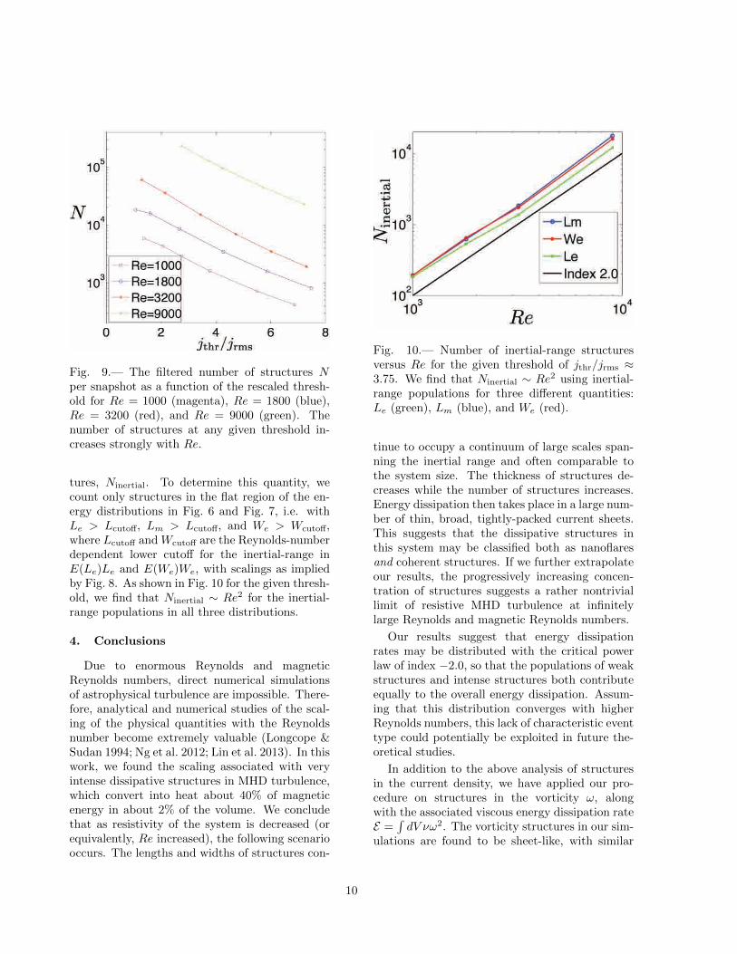
Fig. 9.— The filtered number of structures Nper snapshot as a function of the rescaled thresh-old for Re = 1000 (magenta), Re = 1800 (blue),Re = 3200 (red), and Re = 9000 (green). Thenumber of structures at any given threshold in-creases strongly with Re.

tures, Ninertial. To determine this quantity, wecount only structures in the flat region of the en-ergy distributions in Fig. 6 and Fig. 7, i.e. withLe > Lcutoff, Lm > Lcutoff, and We > Wcutoff,where Lcutoff and Wcutoff are the Reynolds-numberdependent lower cutoff for the inertial-range inE(Le)Le and E(We)We, with scalings as impliedby Fig. 8. As shown in Fig. 10 for the given thresh-old, we find that Ninertial ∼ Re2 for the inertial-range populations in all three distributions.

4. Conclusions

Due to enormous Reynolds and magneticReynolds numbers, direct numerical simulationsof astrophysical turbulence are impossible. There-fore, analytical and numerical studies of the scal-ing of the physical quantities with the Reynoldsnumber become extremely valuable (Longcope &Sudan 1994; Ng et al. 2012; Lin et al. 2013). In thiswork, we found the scaling associated with veryintense dissipative structures in MHD turbulence,which convert into heat about 40% of magneticenergy in about 2% of the volume. We concludethat as resistivity of the system is decreased (orequivalently, Re increased), the following scenariooccurs. The lengths and widths of structures con-

Fig. 10.— Number of inertial-range structuresversus Re for the given threshold of jthr/jrms ≈3.75. We find that Ninertial ∼ Re2 using inertial-range populations for three different quantities:Le (green), Lm (blue), and We (red).

tinue to occupy a continuum of large scales span-ning the inertial range and often comparable tothe system size. The thickness of structures de-creases while the number of structures increases.Energy dissipation then takes place in a large num-ber of thin, broad, tightly-packed current sheets.This suggests that the dissipative structures inthis system may be classified both as nanoflaresand coherent structures. If we further extrapolateour results, the progressively increasing concen-tration of structures suggests a rather nontriviallimit of resistive MHD turbulence at infinitelylarge Reynolds and magnetic Reynolds numbers.

Our results suggest that energy dissipationrates may be distributed with the critical powerlaw of index −2.0, so that the populations of weakstructures and intense structures both contributeequally to the overall energy dissipation. Assum-ing that this distribution converges with higherReynolds numbers, this lack of characteristic eventtype could potentially be exploited in future the-oretical studies.

In addition to the above analysis of structuresin the current density, we have applied our pro-cedure on structures in the vorticity ω, alongwith the associated viscous energy dissipation rateE =

∫dV νω2. The vorticity structures in our sim-

ulations are found to be sheet-like, with similar

10

statistical properties as the current sheets. Thetotal viscous energy dissipation is comparable tobut somewhat less than the resistive energy dis-sipation, consistent with the existence of residualenergy (Wang et al. 2011; Boldyrev et al. 2012).

The methods presented in this work can be ap-plied to MHD simulations with more specializedboundary conditions and forcing mechanisms, in-cluding the line-tied model for the solar coronaand sheared-box model for accretion disks. In-deed, line-tied boundary conditions are thoughtto strongly affect current sheet formation (Ng &Bhattacharjee 1998; Cowley et al. 1997; Zweibel& Li 1987) and magnetic tearing modes (Huang &Zweibel 2009; Delzanno & Finn 2008), particularlyat global scales. It is therefore of interest to deter-mine to what extent our present findings can beextrapolated to large scales and realistic parame-ters in those cases. These methods will also be ap-plied to simulations of the kinematic and dynamicdynamos in order to determine the morphologicaldifferences between structures in the two cases.

This work was supported by the US DOE awardde-sc0003888, the DOE grant de-sc0001794, theNSF grant PHY-0903872, the NSF Center forMagnetic Self-Organization in Laboratory andAstrophysical Plasmas at U. Wisconsin-Madison,and the Science and Technology Facilities Coun-cil (STFC) UK. High Performance Computingresources were provided by the Texas AdvancedComputing Center (TACC) at the University ofTexas at Austin under the NSF-Teragrid ProjectTG-PHY080013N.

REFERENCES

Aschwanden, M. J. 2012, Astronomy & Astro-physics/Astronomie et Astrophysique, 539

Aschwanden, M. J., TARBELL, T., Nightingale,R. W., Schrijver, C. J., Kankelborg, C. C.,Martens, P., Warren, H. P., et al. 2000, TheAstrophysical Journal, 535, 1047E1065

Asgari-Targhi, M. & van Ballegooijen, A. A. 2012,ApJ, 746, 81

Asgari-Targhi, M., van Ballegooijen, A. A., Cran-mer, S. R., & DeLuca, E. E. 2013, Astrophys.J., 773, 111

Biskamp, D. 2003, Magnetohydrodynamic turbu-lence (Cambridge University Press)

Blaes, O. 2013, Space Science Reviews

Boldyrev, S. 2006, Phys. Rev. Lett., 96, 115002

Boldyrev, S., Perez, J. C., & Wang, Y. 2012, inAstronomical Society of the Pacific ConferenceSeries, Vol. 459, Numerical Modeling of SpacePlasma Slows (ASTRONUM 2011), ed. N. V.Pogorelov, J. A. Font, E. Audit, & G. P. Zank,3

Bruno, R., Carbone, V., Veltri, P., Pietropaolo,E., & Bavassano, B. 2001, Planet. Space Sci.,49, 1201

Buchlin, E. & Velli, M. 2007, The AstrophysicalJournal, 662, 701

Chiueh, T. & Zweibel, E. G. 1987, The Astrophys-ical Journal, 317, 900

Cowley, S., Longcope, D., & Sudan, R. 1997,Physics reports, 283, 227

Crosby, N. B., Aschwanden, M. J., & Dennis, B. R.1993, Solar Physics, 143, 275

Dahlburg, R. B., Einaudi, G., Rappazzo, A. F., &Velli, M. 2012, Astron. Astrophys., 544, L20

Delzanno, G. L. & Finn, J. M. 2008, Physics ofPlasmas, 15, 032904

Dmitruk, P. & Gomez, D. O. 1999, The Astro-physical Journal Letters, 527, L63

Einaudi, G. & Velli, M. 1999, Physics of Plasmas,6, 4146

Goldreich, P. & Sridhar, S. 1995, The Astrophys-ical Journal, 438, 763

Goodman, J. & Uzdensky, D. 2008, The Astro-physical Journal, 688, 555

Greco, A., Servidio, S., Matthaeus, W., &Dmitruk, P. 2010, Planet. Space Sci., 58, 1895

Huang, Y.-M. & Zweibel, E. G. 2009, Physics ofPlasmas, 16, 042102

Hudson, H. 1991, Solar Physics, 133, 357

11

Kerscher, M. 2000, in Statistical physics and spa-tial statistics (Springer), 36–71

Leung, T., Swaminathan, N., & Davidson, P. 2012,Journal of Fluid Mechanics, 710, 453

Lin, L., Ng, C. S., & Bhattacharjee, A. 2013, inAstronomical Society of the Pacific ConferenceSeries, Vol. 474, Numerical Modeling of SpacePlasma Flows (ASTRONUM2012), ed. N. V.Pogorelov, E. Audit, & G. P. Zank, 159

Longcope, D. & Sudan, R. 1994, The Astrophysi-cal Journal, 437, 491

Maron, J. & Goldreich, P. 2001, The AstrophysicalJournal, 554, 1175

Mecke, K. R. 2000, in Statistical Physics and Spa-tial Statistics (Springer), 111–184

Muller, W.-C. & Biskamp, D. 2000, Physical Re-view Letters, 84, 475

Muller, W.-C., Biskamp, D., & Grappin, R. 2003,Physical Review E, 67, 066302

Ng, C. & Bhattacharjee, A. 1998, Physics of Plas-mas, 5, 4028

—. 2008, The Astrophysical Journal, 675, 899

Ng, C., Lin, L., & Bhattacharjee, A. 2012, TheAstrophysical Journal, 747, 109

Pariev, V. I., Blackman, E. G., & Boldyrev, S. A.2003, Astron. Astrophys., 407, 403

Parker, E. 1972, Astrophys. J., 174, 499

Parker, E. 1983, The Astrophysical Journal, 264,635

—. 1988, Astrophys. J., 330, 474

Parnell, C. & Jupp, P. 2000, The AstrophysicalJournal, 529, 554

Perez, J. & Boldyrev, S. 2010, Phys. Plasmas, 17,055903

Perez, J. C., Mason, J., Boldyrev, S., & Cattaneo,F. 2012, Physical Review X, 2, 041005

Rappazzo, A., Velli, M., & Einaudi, G. 2010, TheAstrophysical Journal, 722, 65

Rappazzo, A., Velli, M., Einaudi, G., & Dahlburg,R. 2008, The Astrophysical Journal, 677, 1348

Rappazzo, A. F., Velli, M., & Einaudi, G. 2013,Astrophys. J., 771, 76

Schmalzing, J. & Buchert, T. 1997, The Astro-physical Journal Letters, 482, L1

Schmalzing, J., Buchert, T., Melott, A. L., Sahni,V., Sathyaprakash, B., & Shandarin, S. F. 1999,The Astrophysical Journal, 526, 568

Uritsky, V. M., Davila, J. M., Ofman, L., &Coyner, A. J. 2013, The Astrophysical Journal,769, 62

Uritsky, V. M., Pouquet, A., Rosenberg, D.,Mininni, P. D., & Donovan, E. F. 2010, Phys.Rev. E, 82, 056326

Veltri, P. 1999, Plasma Phys. Contr. F., 41, A787

Wang, Y., Boldyrev, S., & Perez, J. C. 2011, TheAstrophysical Journal, 740, L36

Wilkin, S. L., Barenghi, C. F., & Shukurov, A.2007, Physical review letters, 99, 134501

Zhdankin, V., Boldyrev, S., & Mason, J. 2012,The Astrophysical Journal Letters, 760, L22

Zhdankin, V., Uzdensky, D., Perez, J., &Boldyrev, S. 2013, ApJ, 771, 124

Zweibel, E. G. & Li, H.-S. 1987, The AstrophysicalJournal, 312, 423

This 2-column preprint was prepared with the AAS LATEXmacros v5.2.

12