OPTIMAL CONTROL AND DESIGN USING GENETIC ALGORITHMS ACCELERATED BY NEURAL NETWORKS By SARASWATHI NAMBI A THESIS PRESENTED TO THE GRADUATE SCHOOL OF THE UNIVERSITY OF FLORIDA IN PARTIAL FULFILLMENT OF THE REQUIREMENTS FOR THE DEGREE OF MASTER OF SCIENCE UNIVERSITY OF FLORIDA 2011

Welcome message from author
This document is posted to help you gain knowledge. Please leave a comment to let me know what you think about it! Share it to your friends and learn new things together.
Transcript

OPTIMAL CONTROL AND DESIGN USING GENETIC ALGORITHMS ACCELERATEDBY NEURAL NETWORKS
By
SARASWATHI NAMBI
A THESIS PRESENTED TO THE GRADUATE SCHOOLOF THE UNIVERSITY OF FLORIDA IN PARTIAL FULFILLMENT
OF THE REQUIREMENTS FOR THE DEGREE OFMASTER OF SCIENCE
UNIVERSITY OF FLORIDA
2011

c⃝ 2011 Saraswathi Nambi
2

To Vadivazhaghia Nambi Arasappan Pillai
3

ACKNOWLEDGMENTS
I would like to express my gratitude to my mentor Professor Anil V. Rao for
giving me the opportunity to work on this research program. Without his support
and encouragement, this project would have not been possible. I would also like to thank
my committee member, Professor Warren E. Dixon for his inputs and expert guidance
towards my project. It was through him that I got introduced to Neural Networks. I am
grateful to him for teaching me all the concepts involved in Non-Linear Control Theory
and for patiently listening and clarifying all my inquisitive questions. His presence and
encouragement throughout the project is invaluable to me.
I am indebted to Rushikesh Kamalapurkar, who has been assisting me in all
my experiments despite his various research commitments and tight schedules.
Additionally, I wish to take this opportunity to thank all my other colleagues for their
valuable support during my research career.
Finally I wish to express my deepest appreciation to my family and friends for
standing by me in all aspects of my academics and personal life.
4
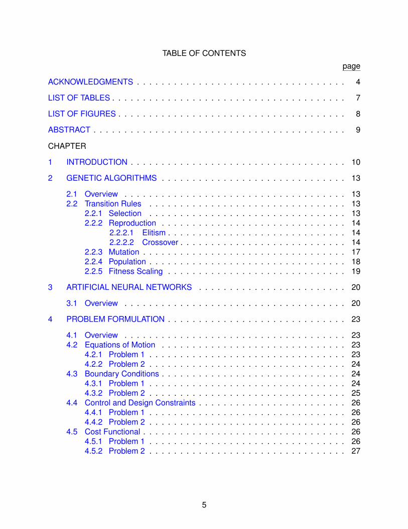
TABLE OF CONTENTS
page
ACKNOWLEDGMENTS . . . . . . . . . . . . . . . . . . . . . . . . . . . . . . . . . . 4
LIST OF TABLES . . . . . . . . . . . . . . . . . . . . . . . . . . . . . . . . . . . . . . 7
LIST OF FIGURES . . . . . . . . . . . . . . . . . . . . . . . . . . . . . . . . . . . . . 8
ABSTRACT . . . . . . . . . . . . . . . . . . . . . . . . . . . . . . . . . . . . . . . . . 9
CHAPTER
1 INTRODUCTION . . . . . . . . . . . . . . . . . . . . . . . . . . . . . . . . . . . 10
2 GENETIC ALGORITHMS . . . . . . . . . . . . . . . . . . . . . . . . . . . . . . 13
2.1 Overview . . . . . . . . . . . . . . . . . . . . . . . . . . . . . . . . . . . . 132.2 Transition Rules . . . . . . . . . . . . . . . . . . . . . . . . . . . . . . . . 13
2.2.1 Selection . . . . . . . . . . . . . . . . . . . . . . . . . . . . . . . . 132.2.2 Reproduction . . . . . . . . . . . . . . . . . . . . . . . . . . . . . . 14
2.2.2.1 Elitism . . . . . . . . . . . . . . . . . . . . . . . . . . . . . 142.2.2.2 Crossover . . . . . . . . . . . . . . . . . . . . . . . . . . . 14
2.2.3 Mutation . . . . . . . . . . . . . . . . . . . . . . . . . . . . . . . . . 172.2.4 Population . . . . . . . . . . . . . . . . . . . . . . . . . . . . . . . . 182.2.5 Fitness Scaling . . . . . . . . . . . . . . . . . . . . . . . . . . . . . 19
3 ARTIFICIAL NEURAL NETWORKS . . . . . . . . . . . . . . . . . . . . . . . . 20
3.1 Overview . . . . . . . . . . . . . . . . . . . . . . . . . . . . . . . . . . . . 20
4 PROBLEM FORMULATION . . . . . . . . . . . . . . . . . . . . . . . . . . . . . 23
4.1 Overview . . . . . . . . . . . . . . . . . . . . . . . . . . . . . . . . . . . . 234.2 Equations of Motion . . . . . . . . . . . . . . . . . . . . . . . . . . . . . . 23
4.2.1 Problem 1 . . . . . . . . . . . . . . . . . . . . . . . . . . . . . . . . 234.2.2 Problem 2 . . . . . . . . . . . . . . . . . . . . . . . . . . . . . . . . 24
4.3 Boundary Conditions . . . . . . . . . . . . . . . . . . . . . . . . . . . . . . 244.3.1 Problem 1 . . . . . . . . . . . . . . . . . . . . . . . . . . . . . . . . 244.3.2 Problem 2 . . . . . . . . . . . . . . . . . . . . . . . . . . . . . . . . 25
4.4 Control and Design Constraints . . . . . . . . . . . . . . . . . . . . . . . . 264.4.1 Problem 1 . . . . . . . . . . . . . . . . . . . . . . . . . . . . . . . . 264.4.2 Problem 2 . . . . . . . . . . . . . . . . . . . . . . . . . . . . . . . . 26
4.5 Cost Functional . . . . . . . . . . . . . . . . . . . . . . . . . . . . . . . . . 264.5.1 Problem 1 . . . . . . . . . . . . . . . . . . . . . . . . . . . . . . . . 264.5.2 Problem 2 . . . . . . . . . . . . . . . . . . . . . . . . . . . . . . . . 27
5

5 AUGMENTATION OF GENETIC ALGORITHMS AND ARTIFICIAL NEURALNETWORKS . . . . . . . . . . . . . . . . . . . . . . . . . . . . . . . . . . . . . 28
5.1 Overview . . . . . . . . . . . . . . . . . . . . . . . . . . . . . . . . . . . . 285.2 Augmentation . . . . . . . . . . . . . . . . . . . . . . . . . . . . . . . . . . 29
6 RESULTS . . . . . . . . . . . . . . . . . . . . . . . . . . . . . . . . . . . . . . . 34
7 CONCLUSION . . . . . . . . . . . . . . . . . . . . . . . . . . . . . . . . . . . . 41
REFERENCES . . . . . . . . . . . . . . . . . . . . . . . . . . . . . . . . . . . . . . . 43
BIOGRAPHICAL SKETCH . . . . . . . . . . . . . . . . . . . . . . . . . . . . . . . . 45
6

LIST OF TABLES
Table page
6-1 GA Parameters for Problem 1 and Problem 2 . . . . . . . . . . . . . . . . . . . 34
6-2 GA Parameters for Problem 1 and Problem 2 . . . . . . . . . . . . . . . . . . . 35
6-3 Optimal Design Parameters obtained using GA and NN . . . . . . . . . . . . . 38
7
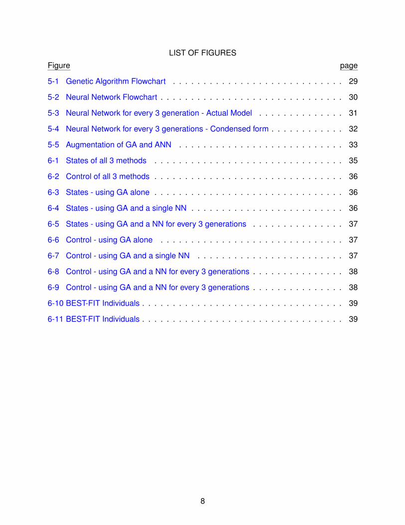
LIST OF FIGURES
Figure page
5-1 Genetic Algorithm Flowchart . . . . . . . . . . . . . . . . . . . . . . . . . . . . 29
5-2 Neural Network Flowchart . . . . . . . . . . . . . . . . . . . . . . . . . . . . . . 30
5-3 Neural Network for every 3 generation - Actual Model . . . . . . . . . . . . . . 31
5-4 Neural Network for every 3 generations - Condensed form . . . . . . . . . . . . 32
5-5 Augmentation of GA and ANN . . . . . . . . . . . . . . . . . . . . . . . . . . . 33
6-1 States of all 3 methods . . . . . . . . . . . . . . . . . . . . . . . . . . . . . . . 35
6-2 Control of all 3 methods . . . . . . . . . . . . . . . . . . . . . . . . . . . . . . . 36
6-3 States - using GA alone . . . . . . . . . . . . . . . . . . . . . . . . . . . . . . . 36
6-4 States - using GA and a single NN . . . . . . . . . . . . . . . . . . . . . . . . . 36
6-5 States - using GA and a NN for every 3 generations . . . . . . . . . . . . . . . 37
6-6 Control - using GA alone . . . . . . . . . . . . . . . . . . . . . . . . . . . . . . 37
6-7 Control - using GA and a single NN . . . . . . . . . . . . . . . . . . . . . . . . 37
6-8 Control - using GA and a NN for every 3 generations . . . . . . . . . . . . . . . 38
6-9 Control - using GA and a NN for every 3 generations . . . . . . . . . . . . . . . 38
6-10 BEST-FIT Individuals . . . . . . . . . . . . . . . . . . . . . . . . . . . . . . . . . 39
6-11 BEST-FIT Individuals . . . . . . . . . . . . . . . . . . . . . . . . . . . . . . . . . 39
8
Abstract of thesis Presented to the Graduate Schoolof the University of Florida in Partial Fulfillment of the
Requirements for the Degree of Master of Science
OPTIMAL CONTROL AND DESIGN USING GENETIC ALGORITHMS ACCELERATEDBY NEURAL NETWORKS
By
Saraswathi Nambi
August 2011
Chair: Anil V. RaoMajor: Aerospace Engineering
The main feature of this paper is the incorporation of Artificial Neural Networks
(ANN) to accelerate the processing time of Genetic Algorithms (GA). In this paper, we
use ANN for data mining and approximation of the initial range required GA such that
its search efficiency increases. Deterministic/Gradient-based methods have proven
to be difficult to produce optimal solutions to problems whose objective functions are
discontinuous, non-differentiable, non-linear and stochastic. On the other hand, GA can
produce an accurate search for an optimal solution for such problems. The hybridization
of a GA with ANN though complex and expensive than the deterministic methods, is
found to be more efficient in regard to actual operation time and near-optimal solutions
for a given optimization problem. The method developed in this paper is a two-stage
approach. The initial population required by GA is obtained using an ANN. Using this
initial population, an optimal solution is obtained by GA. The approach is demonstrated
in two types of problem - an optimal control problem and a fin design problem. It was
found to be a successful method for generating optimal solutions in a constrained
environment with minimal input from the user.
9
CHAPTER 1INTRODUCTION
Over the years several techniques for optimization of aircraft and spacecraft
trajectories have been developed. Optimization theories are not restricted to Aerospace
applications alone but are found in use for Industrial Engineering, Business Management,
Mechanical design and other streams as well [1]. The methods have been largely
classified as gradient-based approach and heuristic approach. Initially theories for
optimization were proposed using mathematical models and later automated tools were
designed, developed and modified to produce solutions for all optimization problems.
The automated optimization tools for numerical methods in recent times have been
known to solve unconstrained, constrained, non-linear, linear, quadratic, non-linear
least squares, sparse and structured objective and multi-objective problems. Extensive
research has been carried out in designing and developing tools for optimization
problems with applications in aerospace engineering. In general, optimization problems
do not have any analytical solutions and are solved using either numerical methods or
heuristic methods. Optimization of a trajectory using global collocation [2] where finite
and infinite horizon problems have been solved using Legendre-Gauss-Radau (LGR)
points. Space trajectories have been optimized using Particle Swarm Optimization
which is a stochastic method inspired by behavior of birds and ants while searching
for food [3]. Similarly a multi-objective problem using deterministic Collaborative
Robust Optimization has been developed and is assisted by an approximation for
uncertain intervals [4]. These researchers used methods involving gradient-based
and deterministic approaches since the objective function was continuous and
differentiable over a specified interval which constrained the solutions to be local.
Problem arises when the objective function in real-time applications are discontinuous
and non-differentiable. In literature, a handful of heuristic techniques have been
published [5],[6], [7],[8]which overcome the disadvantage of gradient-based methods,
10

discontinuous and non-differentiable objectives. A near-optimal solution [9] was
achieved for an Earth-Mars Trajectory using a stochastic approach (Genetic Algorithm).
The literature published was to identify whether a GA Optimizer was suitable for a
realistic model. In fact, a similar approach using collocation and non-linear programming
was solved [10]. The main reason behind the implementation was that GA Optimizer
was simple and required no initial guesses or prior information. Similarly, GA was
developed as a preprocessing algorithm to formulate an initial guess of the solution for a
direct collocation with non-linear programming method (semi-DCNLP). Several articles
based on an augmented GA and ANN have been proposed, of which all problems
pertain to training Neural Network for a particular set of design data (fluid and thermal
science or structures). After the training has been accomplished, the approximated data
is used as the objective to be optimized by GA Optimizer.
To address the problem dealing with objective functions which are not smooth
and have discontinuities or large derivatives, an approach is developed in this paper
such that the solution is optimal and consistent, obtained using Genetic Algorithms
(GA) accelerated by Artificial Neural Networks (ANN). Genetic Algorithms depend
upon natural selection and natural genetics. Initially a set of solutions are created by
random generation and this set is called population. The solution to a specific problem
is chosen from this current population depending on their best fitness. New populations
are created for every generation by choosing the best individuals as parents from
current population and using reproduction, crossover and mutation operators to produce
offspring (individuals) for next generation. Over evolving successive generations, the
population converges to an optimal solution. Moreover an initial guess of solution
or any other input provided by the user is not required for Genetic Algorithms, as is
the case for numerical methods. GA uses an initial range for population and finds an
optimal solution from the population depending upon their best fitness value. If an
initial range is really huge when compared to the range in which the optimal solution
11

lies, GA tends to lead a very slow optimization process which might prolong for many
long hours and never converge to a solution. The other possibility of the range being
too small will result in premature convergence of an optimal solution. So it is highly
essential that a proper initial range is chosen such that evaluations carried out by
GA are inexpensive. Literature works show that determining optimal trajectories and
optimal design parameters of space vehicles in minimal computational time with less
or no input from the user is highly important for improving the efficiency of spacecrafts
and Unmanned Aerial Vehicles (UAVs). In this paper, we solve for optimal solutions
using multi-stage approach heuristically. The solutions for optimal control and design
problems are obtained using a hybrid solver - Genetic Algorithms and Artificial Neural
Networks. ANN generates the initial range for GA from which an initial population is
created randomly. Using this initial range, GA solves for optimal solutions of the control
and design problem. The solutions obtained using this approach are compared with
optimal solutions obtained using numerical methods,hybridization of GA and a single
ANN and GA in the absence of ANN.
12
CHAPTER 2GENETIC ALGORITHMS
2.1 Overview
Genetic Algorithms are heuristic search algorithms based on natural genetics
theory. It was developed by John Holland and his students at University of Michigan
in 1975 [11]. It is an artificial system that follows the mechanisms of natural genetics
and natural selection. The main advantage of this method has been its robustness
and flexibility in complex spaces. It is known for its simplicity which involves copying,
crossing over and mutating the strings. They do not work with the parameters that are
to be optimized but with a coded form of the parameter set. Initially the parameters are
coded to binary strings (individuals). The coding of parameters is not restricted to a
single string but also by applying transition rules (Selection 2.2.1,Reproduction 2.2.2
and Mutation (2.2.3) to generate new strings for each trial. These individuals together
form the initial population of size ’n’, where n is the number of trials used to generate
new strings. This is followed by successive generation of populations. Searching for an
optimal solution in a population of points (parallel computing) reduces the probability of
finding a false solution instead of moving gingerly from a single point to another using
calculus-based transition rule which ultimately leads to location of false solutions in
multimodal search spaces. Taking into consideration the direct coding of parameters,
search from a population of strings, and no need for auxiliary information together
account for the robustness of the GA optimizer.
2.2 Transition Rules
Genetic Algorithms uses three main operators to create successive generations
from current population are:
2.2.1 Selection
These are rules which select the best fit individuals for the given objective. It follows
the artificial version of natural selection - Darwinian theory where individuals with more
13
fit have better potential to survive and most popularly known by the phrase ’survival of
the fittest’. These best fit individuals become the parents of current generation and will
reproduce again to form the next generation.
There are different types of function for the process - Stochastic uniform, Remainder,
Uniform, Roulette and Tournament.
In Stochastic uniform type of function, a line is laid and each parent corresponds to
a section of line which is proportional to its scaled value.
In Remainder function, parents are assigned deterministically from an individual’s
scaled value and roulette selection is used to for the remaining fractional part. After the
parents are assigned, they are chosen stochastically. The probability that a parent is
being chosen in this method is proportional to its fractional part of its scaled value.
As for Uniform function, parents are chosen according to expectations and
number of parents. This method is not an effective search strategy but can be used
for debugging and testing.
In Roulette, parents are chosen using a simulated roulette wheel, where the area of
a section of the wheel (of an individual) is proportional to the individual’s expectation.
The parents in Tournament function are chosen by choosing a random tournament
size and best individuals out of that tournament set are chosen as parents.
2.2.2 Reproduction
This process specifies how the children are being created for the next generation.
They are of two types
2.2.2.1 Elitism
It defines the number of individuals that will survive the next generation and is user
specified and can be denoted as a real number.
2.2.2.2 Crossover
A set of rules which swap the characters or traits between two strings or individuals
which result in partial string exchanges. So crossing randomly selected best-fit
14

individuals result in a new population constructed by varying their traits. There are
different options for crossover function such as Scattered, Single point, Two Point,
Intermediate, Heuristic and Arithmetic.In Scattered option, a random binary string
is created, the ones in the binary string are replaced by the elements of parent1,
corresponding to ones’ position. In a similar manner the zeros of the string are replaced
by the elements of parent2. For example, if
v1 =
[q w e r t y
](2–1)
and
v2 =
[1 2 3 4 5 6
](2–2)
are parents, then the created bit string being
b =
[1 0 1 1 0 0
](2–3)
then the child would be
c =[
q 2 e r 5 6
](2–4)
As for Single point crossover, a random number from 1 to n is chosen, where n is
the number of variables is chosen. Then the vector elements lesser than or equal to the
random number is chosen from parent1, similarly vector elements greater than or equal
to random number is chosen from parent2. These elements are concatenated to form a
child vector. For example, if
v1 =
[q w e r t y
](2–5)
and
v2 =
[1 2 3 4 5 6
](2–6)
If the random number is 4, then the child is
c =[
q w e r 5 6
](2–7)
15
Two-point crossover is similar to Single-point crossover but two random numbers
are selected from 1 to number of variables. Using the same example, if v1 and v2 are
parents, then
v1 =
[q w e r t y
](2–8)
and
v2 =
[1 2 3 4 5 6
](2–9)
If the random number is 2 and 4, then the child is
c =[
q w 3 4 t y
](2–10)
In Intermediate crossover, the child is created by using the weighted average of the
parents. The weight is user-defined and is a single parameter which can be a scalar or a
vector. The following formula is used to create the child.
c1 = v1 + p(v2 − v1) (2–11)
where c1 is the child, p is the weight, v2 is parent2, and v1 is parent1. If the weight lies
between the range [0,1], the children generated lie within the hypercube created by
parents who are placed in opposite vertices. If otherwise, the children lie outside the
hypercube generated. If the weight is a scalar, then the children lie in the same line
connecting the vertices.
As for Heuristic method, the children lie in a line containing the two parents, a
very small distance from the better fitted parent and away from the worst fitted parent.
The distance from the better fitted parent is user defined and this function follows the
equation
c1 = v2 +h(v1 − v2) (2–12)
where c1 is the child, h is the distance from parent1, v2 is parent2 (worst-fitted), and v1 is
parent1 (better-fitted). In the Arithmetic option, the children are reproduced which are the
16

weighted mean of the actual parents. These children are always feasible even with linear
constraints and bounds.
2.2.3 Mutation
Mutation is a set of rules which randomly alters the value in a string. It is needed
because of the fact that crossover and selection occasionally may lose potentially
useful information retained in a string. The different types of mutation are Gaussian and
Uniform.
In the Gaussian type, a Gaussian distribution is created with a mean of zero. A
random number is chosen from this distribution and added to the entries of the parent.
The distribution is created using the initial range specified by the user. So if the initial
range is a vector of two rows and columns equal to the number of variables, then a
standard deviation is generated using the formula
SD = psd (vi,2 − vi,1) (2–13)
where psd is a parameter defined by the user which can be an integer and determines
the initial value of standard deviation in the first generation, v2 is parent2, v1 is parent1
and i is the co-ordinate corresponding to the parent vectors.
Another parameter gsd determines or controls the spread of the standard deviation.
The standard deviation for kth is given by
SDi,k = SDi,k−1
(1−gsd
kgenerations
)(2–14)
where i is the co-ordinate corresponding to the parent vectors.
In the Uniform Mutation process, initially a fraction of vector entries of the parents
are chosen for mutation and each entry has a probability rate of being mutated. After
the entries are chosen, they will be replaced by a random number selected (uniform
selection) from the range of that entry.
17
There are other Genetic operators as well; however the above three are the main
operators which have proved to be effective and efficient in solving many optimization
problems. The three main parameters which decide upon the efficiency of a GA
Optimizer are the population, cross-over fraction and mutation. The nominal rates
for cross-over and mutation are 0.8 and 0.035 respectively. It is a known fact that GA
performance requires the choice of a high crossover probability and a low mutation
property and a moderate population size.
2.2.4 Population
The population size defines how many individuals are generated for each
generation. The determination of population occurs from a predefined initial population
range. The initialrange can be user defined and it specifies the range of the vectors
in the initial population that is to be generated. It is of utmost importance because of
the fact the search space is a function of the initial range. If the given search space is
large enough, the solutions of GA are known to be smooth and unimodal or if the search
space is not large enough, it would conduct an exhaustive search and find a solution,
but it would be a local optimum rather than global optimum and if the search space
is exorbitantly large the GA would continue solving and eventually would take infinite
time to arrive at an optimal solution. The types of population for the entries can be
generated as bit strings or vectors. If the population is a vector, multiple subpopulations
are generated which equals the length of the vector defined. In such case, Migration
specifies how many individuals are passed on to the next generation. The worst
individuals of a specific population are replaced by the best individuals of another
population. There are three types of possible ways in which migration can be carried out
- by Direction, Interval and Fraction.
Direction - as the name indicates, the direction in which the migration should
take place is specified. It can either be forward or both. If migration is to take from nth
generation, then in forward migration, n+ 1th generation is replaced by nth generation.
18

If the migration takes place in both directions then the n+ 1th generation and n− 1th
generation are replaced by nth generation.
Interval - The migration takes place after a specific interval. If the interval is chosen
to be 10 then migration takes place every 10 generations of the optimization process.
Fraction - The number of individuals which can migrate between populations is
defined by the fraction function.
2.2.5 Fitness Scaling
The fitness function values which are being returned after each generation can
be scaled. Raw fitness scores will be returned by the fitness function and they can
be scaled down to values which will be suitable for the selection function and this is
called fitness scaling. The different types of fitness scaling are rank, proportional, and
shift linear. In the type rank, the raw score are scaled according their rank (its position
depending on sorted scores). This type of scaling removes effect of spread of the
scores. In proportional scaling the scaled value of an individual is proportional to its raw
fitness score. As for shift linear, the raw scores are scaled such that the expected fittest
individual is equal to a constant (user defined) multiplied by average fitness score.
The above said parameters are the different options with which a Genetic
Algorithm Optimizer can be designed. Parameters can also be user defined and
custom made according to a specific problem. The discussed options are the most
commonly defined and essential options. These clearly define the rules using which
an optimization process can be carried out without any discrepancies. They improve
the performance of the function towards an optimal point i.e. an approach which
leads to improvement towards an optimal point. Calculus-based methods have always
focused on convergence and not on the interim performance. On the contrary, Genetic
Algorithms strive to improve the fitness function using the above discussed options to
attain an optimal solution.
19
CHAPTER 3ARTIFICIAL NEURAL NETWORKS
3.1 Overview
Artificial Neural Networks are mathematical models of human nervous system.
They are composed of artificial neurons or nodes. The effect of synaptic terminals is
carried out by weight functions which modulate the effect of inputs and the nonlinearity
of the nodes is represented by a transfer function. The inputs defined here in the picture
are equivalent to inputs received by the dendrites of a human neuron and the output
transmitted is equivalent to the output transmitted by the axon of a human neuron. The
output of the artificial neuron is given by the Universal Approximation Property
yi =W ·σ(b,xi)+ ε (3–1)
where W is the weight vector, x is the input vector, bias weight b, ε is the approximation
error and σ is the activation function. The transmission of signals is calculated as a
weighted sum of the inputs and is transformed by the transfer function. By altering
the values of the weights a neural network can be trained to perform a particular
function. They can be essentially trained to perform different functions such as fitting
a function, recognizing a pattern, clustering datasets, approximation of data and
controlling systems. The transfer functions or the activation functions are mainly
classified by three types. They are Step function, Linear function and Sigmoid function.
The Step function returns zero if the output is equal to zero or lesser than zero and
returns one if it is greater than zero. It represented by the equation
y =
1 if x ≥ 0
0 if x < 0(3–2)
where y is the output function and x is the input function.
The Linear Transfer Function usually spans between −∞ to +∞ and denoted by
straight line. It is a function of a single variable input. It output is same as the input or a
20

function of addition and multiplication of the input. The equation which represents the
function is given by
y = mx+ c (3–3)
where m and c are real constants, y the output and x the input.
As for the Sigmoid function, is a progressive function which spreads from small
values and within given period of time accelerates to reach a maximum value. The
equation which represents the function is given by
y(x) =1
1+ e−x (3–4)
where, y the output and x the input.
A basic neural network has three layers namely input layer, hidden layer and output
layer. The input layer can be a scalar input or input of vectors. Here the hidden layer
is function of the weights w and bias b. An ANN is to be designed such that the inputs
produce a desired output and this wholly depends upon the weights of the network.
Various methods exist to strengthen the connection; one of them is to set the weights
explicitly and another is that by training the neural networks and using a learning rule.
In this particular paper we are using Radial Basis Neural Networks to carry
out approximation of initial range from the generation data obtained from GA. The
approximation of the generation data results in gives an estimate set of values for the
next generation, from which an initial range for the next generation can be deduced. The
Radial Basis Neural Network has three layers namely input, hidden radial basis layer
and output linear layer. The Radial Basis Function is a Gaussian distribution which is
mainly known for its approximation technique in statistics. The Neural Network used in
this literature is for the same approximation of clustered data. The entire working of the
neural net is explained in this chapter.
The net input to the transfer function is that the vector distance between cluster
center c and input vector x multiplied by bias b. This type of setting weights is called
21

clustering technique. The concept is that patterns present in the input vector form
clusters. The center of the clusters is known and the Euclidean distance between the
input vector and the cluster center is measured. As the input moves away from the
center, the activation value reduces. The transfer function is given as
σ(b,x) = e−n (3–5)
where n = ∥c− x∥ · b is the coefficient of the transfer function of the hidden layer, c is the
center of the cluster, x is the input vector, b is the spread of the transfer function.
The radial basis function has a maximum of 1 when the input is 0, i.e. it produces
1 when the input x is equal to its weight w. The bias vector b allows the sensitivity of
the radial basis neuron to be adjusted. The factor n = ∥c− x∥ · b is the weight of the
layer which is a width parameter that controls the spread of the curve. The hidden layer
transforms the inputs to a nonlinear function from the input space to the hidden space,
whereas the output layer applies a linear space from hidden to output space. The hidden
layer uses the Radial Basis Function while the output uses Linear Function.
The use of this approximation to approximate the values obtained after the initial run
of the Genetic Algorithms Solver for determining the range of initial population will be
discussed in detail in the coming chapter.
22
CHAPTER 4PROBLEM FORMULATION
4.1 Overview
There are are two kind of problems solved in this paper to test the working of the
proposed algorithm, developed using MATLAB. The objective of one problem is to find
the optimal trajectory of a moving vehicle using the control angle and the other problem
deals with finding an optimal trajectory of a model rocket using the fin design. The
problem formulation for the design of optimal trajectory is as follows.
• In Section (4.2), the equations of motion are formulated.
• In Section (4.3), the boundary conditions are developed.
• In Section (4.4), the control constraints are formulated.
• Section (4.5), describes the objective function that is to be minimized.
4.2 Equations of Motion
4.2.1 Problem 1
The equations of motion for the vehicle moving at a velocity a over flat Earth are
given as follows
x = u (4–1)
y = v (4–2)
u = acos(β) (4–3)
v = asin(β) (4–4)
where x(t) and y(t) are the horizontal and vertical components of position, u and v
are the horizontal and vertical components of velocity a. β is the control angle.
23

4.2.2 Problem 2
The equations of motion for the model rocket with propellant mass m and total
mass, M, with thrust T acting on it, with a drag of D, and moving with an acceleration a
is given by
y =T (t)−m(t,a) g−D(t)
m(t,a)(4–5)
where the Drag equation is given by
D =12
ρ v2 SiCdi (4–6)
the Thrust is given by
T = m ve (4–7)
the mass flow rate of the propellant is given by
m =m (a−g)−D ve
2
ve(4–8)
where y(t) is the vertical component of position, v is the velocity, a is the acceleration
of the rocket. ve is the exit velocity of the propellant with respect to the rocket, Si is
the surface area of the rocket parts and CD is the co-efficient of drag, D and g is the
acceleration due to gravity.
4.3 Boundary Conditions
4.3.1 Problem 1
The boundary conditions for the vehicle are given as follows
x(t0) = 0 (4–9)
y(t0) = 0 (4–10)
u(t0) = 0 (4–11)
v(t0) = 0 (4–12)
24

where t0 is the initial time. Next, the terminal conditions of each conditions of each
aircraft are given as
x(t f)= x f (4–13)
y(t f)= y f = 0 (4–14)
u(t f)= u f (4–15)
v(t f)= v f = 0 (4–16)
where t f = 10 is the final time of the moving vehicle.
4.3.2 Problem 2
The boundary conditions for the rocket are given as follows
y(t0) = 0 (4–17)
v(t0) = 0 (4–18)
a(t0) = 0 (4–19)
where t0 is the initial time. Next, the terminal conditions of each conditions of each
aircraft are given as
y(t f)= y f = 0 (4–20)
v(t f)= v f (4–21)
a(t f)= a f = 0 (4–22)
where t f = 13 seconds is the final time of the moving vehicle.
25

4.4 Control and Design Constraints
4.4.1 Problem 1
The polynomial used for parameterizing the control angle β is given by
β ≈N
∑i=0
ci ϕi (t) (4–23)
where ϕ(t) = 1+ t + t2 + .... and ci is some constant.
4.4.2 Problem 2
The design constraints for designing the fin of the model rocket is given by the
center of gravity and center of pressure.
The center of pressure is the point on the rocket where all of the aerodynamic
forces act. This was determined by simplifying the traditional calculations. The center of
pressure times the total projected area, A, is equal to the sum of the center of pressure
of each component, d, times the projected area of each component,a
Cp A = anosednose +a f uselaged f uselage +a f insd f ins (4–24)
The center of gravity was computed using the basic equations for determining the
center of mass of an object with multiple components.
CG = ∑ mi di
M(4–25)
where the total mass of the object, M, is equal to the sum of the product of each
individual components mass, m, with its corresponding distance, d, from a reference line.
4.5 Cost Functional
4.5.1 Problem 1
The cost functional for the moving vehicle is to maximize its final horizontal position,
which is given by
J =−xt f (4–26)
26
4.5.2 Problem 2
The cost functional for the rocket is a combination of the static margin,SM and
height of apogee, given by
J =
√(1500− y
1500
)2
+
(2−SM
SM
)2
(4–27)
Using these cost functionals the trajectories of both the problems are determined
subject to the dynamic constraints(Section (4.2)), boundary constraints(Section (4.3)),
control and design constraints (Section (4.4)). The optimal problems are solved using
MATLAB and Simulink version of Genetic Algorithm and Neural Networks using default
feasibility and optimality tolerances.
27

CHAPTER 5AUGMENTATION OF GENETIC ALGORITHMS AND ARTIFICIAL NEURAL
NETWORKS
5.1 Overview
Over the years, many works in literature have amalgamated Neural Networks
with Genetic Algorithms. Most of these literary works have been used in the fields of
Aerospace Engineering [14],[20],[12], Computational Fluid Dynamics [13],[15], Solid
Mechanics [19] or other Design problems [17], [18]. The general outlines of these
problems have been that an optimal design has been achieved by approximating the
results obtained from the Genetic Algorithm using Neural Networks. These works
which have also been optimized by Neural Networks alone or the data obtained using
Genetic Algorithm have been used for training the Neural Networks and then creating
an off-line method to obtain optimal solutions. As far as this research is concerned,
the optimization is carried out by Genetic Algorithms and the approximation is done by
Neural Networks, but a novel way is being implemented. The problem addressed here
is a) processing time and b) consistency of producing near-optimal solutions of Genetic
Algorithms. Though there are several papers which have previously addressed the
same problem [16] but the solutions provided are different. In [16] the objective function
values from Genetic Algorithms are stored in a database and then are approximated to
function or set of values and then strings are selected from this particular approximation.
The main feature to be noted is that objective values obtained from approximation are
inserted in the population set of every generation and the values are again obtained for
every modified generation. Through this solution is feasible and makes perfect sense,
it seems to highly expensive and still accounts to take up much of the processing time.
Secondly, the idea of spoiling the entire population is hindering the main idea of natural
selection and reproduction of genetics. The main design of this paper is that the data
obtained from the GA Optimizer is approximated by a Neural Network to determine
28

the initial range of the population of a GA, thereby not hindering the natural theory of
genetics and building an inexpensive algorithm to carry out the process.
5.2 Augmentation
Firstly a Genetic Algorithm Optimizer is built according to the user’s definition.
To implement a search for optimal solution all parameters of the problem are initially
coded into a chromosome or string where each parameter is a part of the string. The
Figure 5-1. Genetic Algorithm Flowchart
algorithm for generating a GA Optimizer is as follows:
• Step 1: As discussed before a random initial population of strings is generated.
• Step 2: The fitness of each string/chromosome is calculated.
• Step 3: The strings are checked for end-conditions. If they have been met, thestrings are selected as ’best-fit’ individuals for final population; else they areselected to generate a new population.
29
• Step 4: A population is generated using selection, crossover, and mutationoperators.
• Step 5: Two strings are selected as parents based on their fitness value togenerate new set of offspring.
• Step 6: A crossover probability is used to carry out crossover function between thetwo parents to generate a new offspring.
• Step 7: A mutation probability is used to mutate the new offspring generated.
• Step 8: Close-the loop; go to Step 2.
After the best-fit individuals are obtained they are decoded to their original values.
The factors which were taken into consideration for developing a GA Optimizer were
Selection, Reproduction, Mutation and Population.
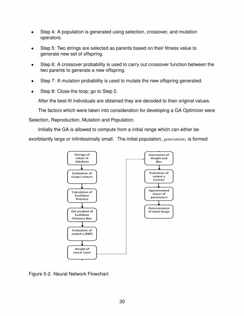
Initially the GA is allowed to compute from a initial range which can either be
exorbitantly large or infinitesimally small. The initial population, generation1 is formed
Figure 5-2. Neural Network Flowchart
30

from the initial range specified in the solver and can be considered to be range of
generation0. Similarly, Genetic Algorithms is allowed to compute generation2 from
generation1 following the transition rules. Using,
x = generation0 as the input vector and (5–1)
t = generation1 as the targetvector (5–2)
a Neural Network is built with a hidden layer using the transfer function
σ(V,x) = e−n (5–3)
where n = ∥c− x∥ · V is the coefficient of the transfer function of the hidden layer, c is the
center of the cluster, x is the input vector, V is the weight of the transfer function.
Figure 5-3. Neural Network for every 3 generation - Actual Model
Now the size of the transfer function is determined. Let nr and nc be the respective
values for number of rows and number of columns. Using this information, the weights of
the network are determined using
t =[W ε
]×
σ(V,x)
ones(1,nc)
(5–4)
31
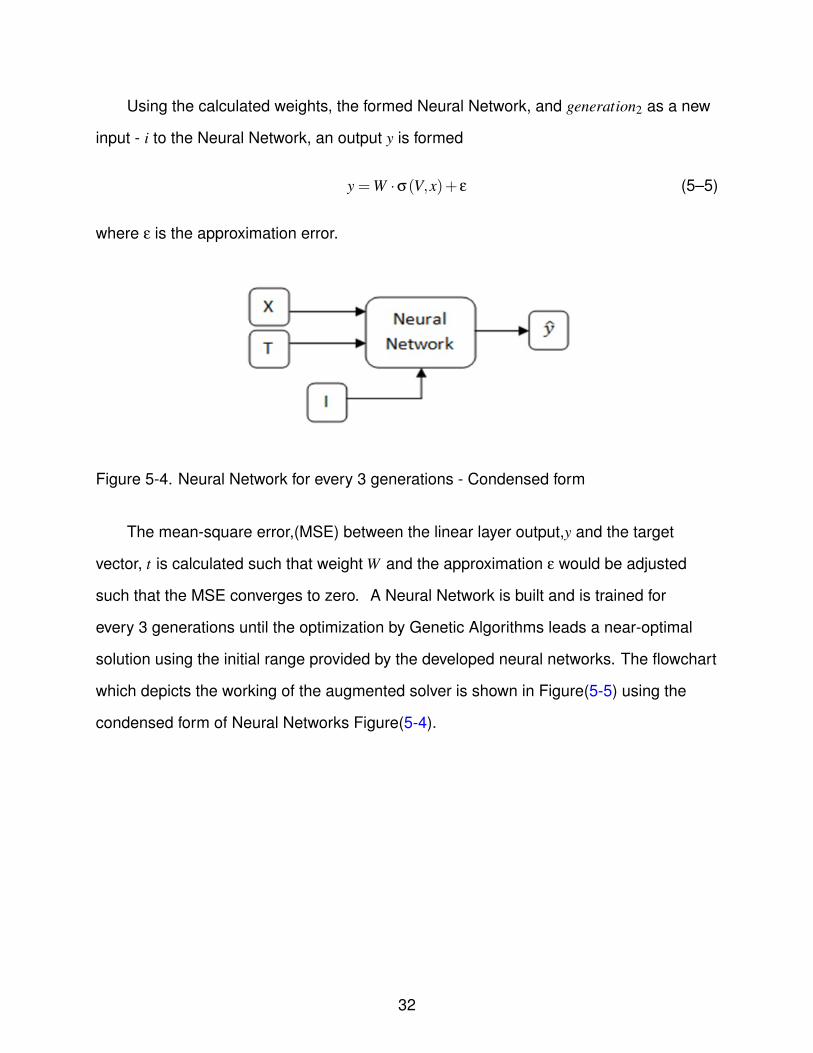
Using the calculated weights, the formed Neural Network, and generation2 as a new
input - i to the Neural Network, an output y is formed
y =W ·σ(V,x)+ ε (5–5)
where ε is the approximation error.
Figure 5-4. Neural Network for every 3 generations - Condensed form
The mean-square error,(MSE) between the linear layer output,y and the target
vector, t is calculated such that weight W and the approximation ε would be adjusted
such that the MSE converges to zero. A Neural Network is built and is trained for
every 3 generations until the optimization by Genetic Algorithms leads a near-optimal
solution using the initial range provided by the developed neural networks. The flowchart
which depicts the working of the augmented solver is shown in Figure(5-5) using the
condensed form of Neural Networks Figure(5-4).
32

Figure 5-5. Augmentation of GA and ANN
33
CHAPTER 6RESULTS
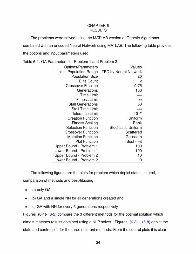
The problems were solved using the MATLAB version of Genetic Algorithms
combined with an encoded Neural Network using MATLAB. The following table provides
the options and input parameters used
Table 6-1. GA Parameters for Problem 1 and Problem 2Options/Parameters Values
Initial Population Range TBD by Neural NetworkPopulation Size 20
Elite Count 2Crossover Fraction 0.75
Generations 100Time Limit +∞
Fitness Limit -∞Stall Generations 50
Stall Time Limit +∞Tolerance Limit 10−6
Creation Function UniformFitness Scaling Rank
Selection Function Stochastic UniformCrossover Function Scattered
Mutation Function GaussianPlot Function Best - Fit
Upper Bound - Problem 1 100Lower Bound - Problem 1 -100Upper Bound - Problem 2 10Lower Bound - Problem 2 0
The following figures are the plots for problem which depict states, control,
comparison of methods and best-fit,using
• a) only GA,
• b) GA and a single NN for all generations created and
• c) GA with NN for every 3 generations respectively.
Figures (6-1)- (6-2) compare the 3 different methods for the optimal solution which
almost matches results obtained using a NLP solver. Figures (6-3) - (6-8) depict the
state and control plot for the three different methods. From the control plots it is clear
34
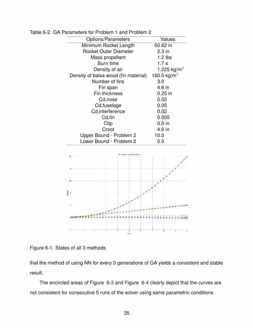
Table 6-2. GA Parameters for Problem 1 and Problem 2Options/Parameters Values
Minimum Rocket Length 50.62 inRocket Outer Diameter 2.3 in
Mass propellant 1.2 lbsBurn time 1.7 s
Density of air 1.225 kg/m3
Density of balsa wood (fin material) 160.0 kg/m3
Number of fins 3.0Fin span 4.6 in
Fin thickness 0.25 inCd,nose 0.02
Cd,fuselage 0.05Cd,interference 0.02
Cd,fin 0.005Ctip 0.0 in
Croot 4.6 inUpper Bound - Problem 2 10.0Lower Bound - Problem 2 0.0
Figure 6-1. States of all 3 methods
that the method of using NN for every 3 generations of GA yields a consistent and stable
result.
The encircled areas of Figure 6-3 and Figure 6-4 clearly depict that the curves are
not consistent for consecutive 5 runs of the solver using same parametric conditions.
35

Figure 6-2. Control of all 3 methods
Figure 6-3. States - using GA alone
Figure 6-4. States - using GA and a single NN
36
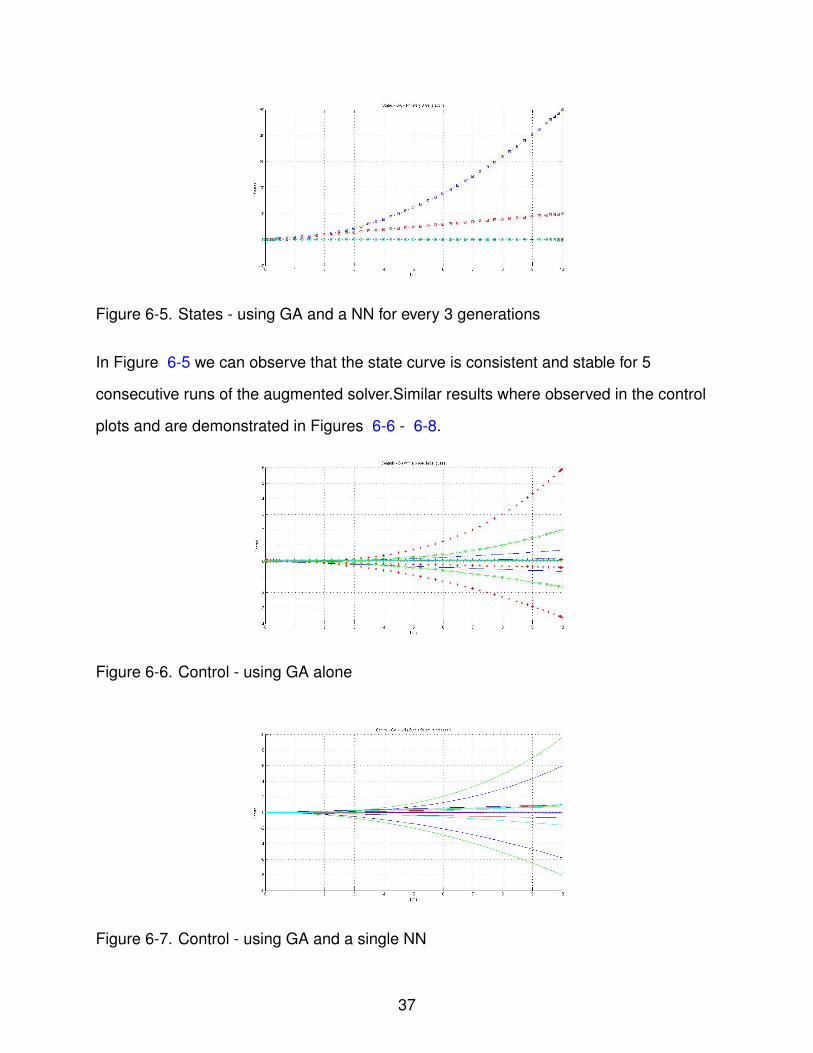
Figure 6-5. States - using GA and a NN for every 3 generations
In Figure 6-5 we can observe that the state curve is consistent and stable for 5
consecutive runs of the augmented solver.Similar results where observed in the control
plots and are demonstrated in Figures 6-6 - 6-8.
Figure 6-6. Control - using GA alone
Figure 6-7. Control - using GA and a single NN
37
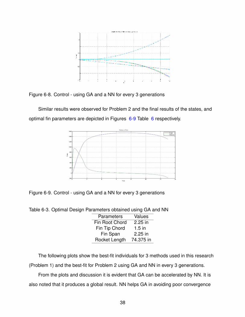
Figure 6-8. Control - using GA and a NN for every 3 generations
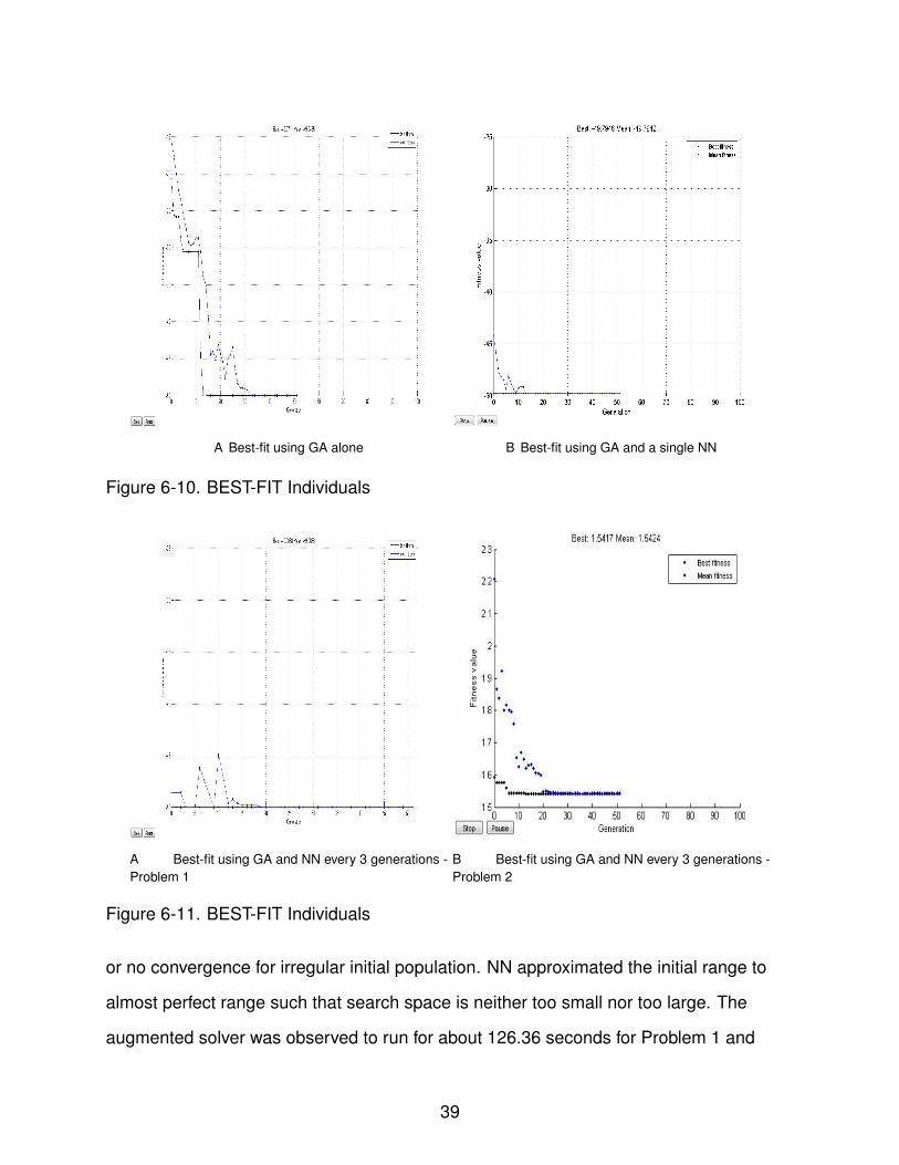
Similar results were observed for Problem 2 and the final results of the states, and
optimal fin parameters are depicted in Figures 6-9 Table 6 respectively.
Figure 6-9. Control - using GA and a NN for every 3 generations
Table 6-3. Optimal Design Parameters obtained using GA and NNParameters Values
Fin Root Chord 2.25 inFin Tip Chord 1.5 in
Fin Span 2.25 inRocket Length 74.375 in
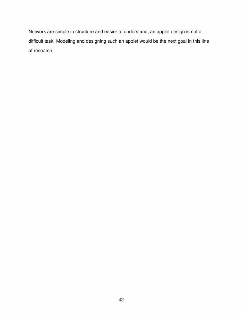
The following plots show the best-fit individuals for 3 methods used in this research
(Problem 1) and the best-fit for Problem 2 using GA and NN in every 3 generations.
From the plots and discussion it is evident that GA can be accelerated by NN. It is
also noted that it produces a global result. NN helps GA in avoiding poor convergence
38
A Best-fit using GA alone B Best-fit using GA and a single NN
Figure 6-10. BEST-FIT Individuals
A Best-fit using GA and NN every 3 generations -Problem 1
B Best-fit using GA and NN every 3 generations -Problem 2
Figure 6-11. BEST-FIT Individuals
or no convergence for irregular initial population. NN approximated the initial range to
almost perfect range such that search space is neither too small nor too large. The
augmented solver was observed to run for about 126.36 seconds for Problem 1 and
39

134.61 seconds for Problem 2, less than using a Genetic Algorithms which takes
about several hours before it converges to a solution. From these results it is evident
that the augmentation of Genetic Algorithms and Neural Networks yields a consistent
near-optimal solution using very little computational time.
40

CHAPTER 7CONCLUSION
From the plots and discussion it is clear that an implementation of approximation
by Neural Network to accelerate Genetic Algorithms is feasible. Apart from that it
produces a global optimal result and is inexpensive as the other methods defined in
literature. The values obtained for Problem 2 were used to design the fin for the rocket
and the rocket had a successful flight and reached a maximum height of 1507 feet. The
Genetic Algorithm accelerated by Neural Networks deduced the maximum height to
be 1543 feet. As for the Problem 1, it had a local optimal solution deduced using Direct
Shooting Method and when Genetic Algorithms with NN was used a global optimal
solution was obtained. It is clear from the results that Genetic Algorithms is capable of a
global solution and to avoid its poor convergence or no convergence for irregular initial
population ranges the augmentation of Neural Networks proved to be successful. The
Neural Networks has approximated the initial range to almost perfect range such that the
search space is neither too large nor too small; it is tailor-made for both the problems
discussed in this paper. In Chapter 2, Genetic Algorithms were discussed in detail along
with the options used in solving the optimization problems. Chapter 3 gave an overview
of Artificial Neural Networks and the specific NN used for approximation purposes.
In Chapter 4, the optimal control and optimal design problems were formulated and
described. Chapter 5 discussed the method of hybridization and the results of the
problems of Chapter 4. In one problem we developed a solution for optimal control and
in the other we developed a solution for optimal design but the objective for both the
problems were such that maximum distance had to be covered.
In order to improve the feasibility of the optimizer, better user-defined applets can be
designed. So to improve the accessibility, the augmentation can be used as a baseline
to develop a Java Applet for control engineers who wish to optimize trajectories or
design objects or design a business project. Since the Genetic Algorithm and Neural
41
Network are simple in structure and easier to understand, an applet design is not a
difficult task. Modeling and designing such an applet would be the next goal in this line
of research.
42
REFERENCES
[1] D. Kirk, ”Optimal control theory: an introduction,”. Dover Publications, 2004.
[2] P. M. F. C. Garg, D., “Direct trajectory optimization and costate estimation offinite-horizon and infinite-horizon optimal control problems using a radaupseudospectral method,” Computational Optimization and Applications, vol. 49, pp.1 – 24, 2009.
[3] M. Pontani and B. CONWAY, “Particle swarm optimization applied to spacetrajectories,” Journal of Guidance, Control, and Dynamics, vol. Vol. 33, No. 5,, pp.pp. 1429–1441., 2010.
[4] M. Emmerich and B. Naujoks, “Metamodel-assisted multiobjective optimisationstrategies and their application in airfoil design,” Adaptive Computing in Design andManufacture, vol. 6, p. pp. 249260., 2004.
[5] K. Horie and B. Conway, “Genetic algorithm preprocessing for numerical solution ofdifferential games problems,” Journal of Guidance, Control and Dynamics, vol. Vol. 27,No. 6, p. pp. 1075., 2004.
[6] H. Y. Peng, F. and A. Ng, “Tests of inflatable structure shape control using geneticalgorithm and neural network,” Proc. AIAA/ASME/ASCE/AHS/ASC Struc. Struct. Dyn.Mat. Conf, vol. Vol.5, p. pp. 31283136., 2005.
[7] P. R. WHITAKER, K.W. and R. MARKIN, “Specifying exhaust nozzle contoursin real-time using genetic algorithm trained neural networks,” AIAA Journal, vol.Vol.31,Issue 2, pp. pp 273–277, 1993.
[8] L. H. K. J. Chen, H.P., “Delamination detection problems using a combined geneticalgorithm and neural network technique,” in 10th AIAA/ISSMO Multidisciplinary Analysisand Optimization Conference, 2004.
[9] B. Wall and B. Conway, “Near-optimal low-thrust earth-mars trajectories via agenetic algorithm,” Journal of Guidance Control and Dynamics, vol. Vol. 28, No. 5, p. pp.1027., 2005.
[10] S. Tang and B. Conway, “Optimization of low-thrust interplanetary trajectories usingcollocation and nonlinear programming,” Journal of Guidance, Control, and Dynamics,vol. Vol. 18, No. 3, pp. pp. 599–604., 1995.
[11] D. Goldberg, ”Genetic algorithms in search, optimization, and machine learning,”.Addison-wesley, 1989.
[12] H. L. S. Z. Q. K. A. . N. K. Rafique, A. F., “Multidisciplinary design and optimizationof an air launched satellite launch vehicle using a hybrid heuristic search algorithm,”Engineering Optimization, vol. Vol. 43, pp. pp. 305–328, 2011.
43
[13] A. Abraham, “Meta learning evolutionary artificial neural networks,” Neurocomputing,vol. Vol. 56, pp. pp. 1–38., 2004.
[14] L. A. N. L. Canavan, G.H., U. S. D. of Energy. Office of Scientific, andT. Information, “Optimal detection of near-earth objects,” Los Alamos NationalLaboratory; distributed by the Office of Scientific and Technical Information, U.S. Dept. ofEnergy, Los Alamos, N.M.; Oak Ridge, Tenn.,, p. pp. 10., 1997.
[15] G. Coupe and T. H. Delft, “On the design of near-optimum control procedures withthe aid of the lyapunov stability theory,” Delft, p. pp. 247., 1975.
[16] R. Duvigneau and M. Visonneau, “Hybrid genetic algorithms and artificial neuralnetworks for complex design optimization in cfd,” International Journal for NumericalMethods in Fluids,, vol. Vol. 44, No. 11, pp. pp. 1257–1278., 2004.
[17] T. Kobayashi and D. Simon, “Hybrid neural-network genetic-algorithm technique foraircraft engine performance diagnostics,” Journal of Propulsion and Power, vol. Vol. 21,No. 4, pp. pp. 751–758, 2005.
[18] E. LaBudde, “A design procedure for maximizing altitude performance,” Researchand Development Project Submitted at NARAM,, pp. pp. 1–34, 1999.
[19] A. Mannelquist, “”near-field scanning optimal microscopy and fractalcharacterization with atomic force microscopy and other methods,”,” Ph.D.dissertation, Lule University of Technology,, 2000.
[20] M. W. K. K. Patre, P., “”asymptotic tracking for uncertain dynamic systems viaa multilayer nn feedforward and rise feedback control structure,”,” IEEE, pp. pp.5989–5994., 2007.
44

BIOGRAPHICAL SKETCH
Saraswathi Nambi is a Graduate Student in Aerospace Engineering at University
of Florida (UF). Her research interests encompass various fileds like trajectory
optimization, neural networks, genetic algorithms and robot design.
Currently, she is involved in optimizing neuronal networks of human brains, signal
processing and optimal control using different heuristic and calculus-based methods.
She aims to work as a Controls Engineer for organizations in areas such as aerospace,
robotics, bioengineering and automation in the future.
45