Naïve Bayes, Maximum Entropy and Text Classificationcs134/TextClassification-NB-MaxEnt.pdf · Text Classification COSI 134. Two RVs: Intelligence(I) and SAT(S) Val(I) = {High,Low},

Naïve Bayes, Maximum Entropy and Text Classification

COSI 134

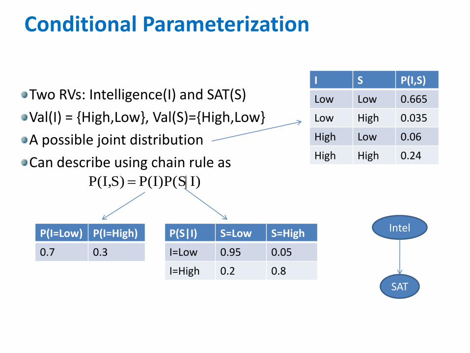
Two RVs: Intelligence(I) and SAT(S)

Val(I) = {High,Low}, Val(S)={High,Low}

A possible joint distribution

Can describe using chain rule as

Conditional Parameterization

I S P(I,S)

Low Low 0.665

Low High 0.035

High Low 0.06

High High 0.24

I)|P(I)P(SS)P(I,

P(I=Low) P(I=High)

0.7 0.3

P(S|I) S=Low S=High

I=Low 0.95 0.05

I=High 0.2 0.8

Intel

SAT

Assume another RV, Grade(G)

Grade in some course

Val(G)={High, Medium, Low}

Might assume that G is conditionally independent of S given I

Then:

Another CPT for

More compact than full joint

Possible to update joint with new information

Conditional IndependenceIntel

SAT Grade

I)|P(GS)I,|P(G

I)P(I)|I)P(G|P(S G)S,P(I, So,

I)|I)P(G|P(SI)|GP(S, indep. cond.By

I)P(I)|GP(S,G)S,P(I,

I)|P(GP(G|I) G=High G=Med G=Low

I=Low 0.2 0.34 0.46

I=High 0.74 0.17 0.09

Four Questions

1) What is the form of the model?

What random variables? How are probabilities computed? What distributions? What parameters?

2) Given a set of data (items from the sample space), how is the likelihood of that data computed, for the given model structure and parameter values?

3) Given a likelihood function, how are the “optimal” parameters estimated given a set of data?

4) Given a model form and a set of induced parameter values, how is inference performed in the model to make predictions/ask queries

Statistical Modeling

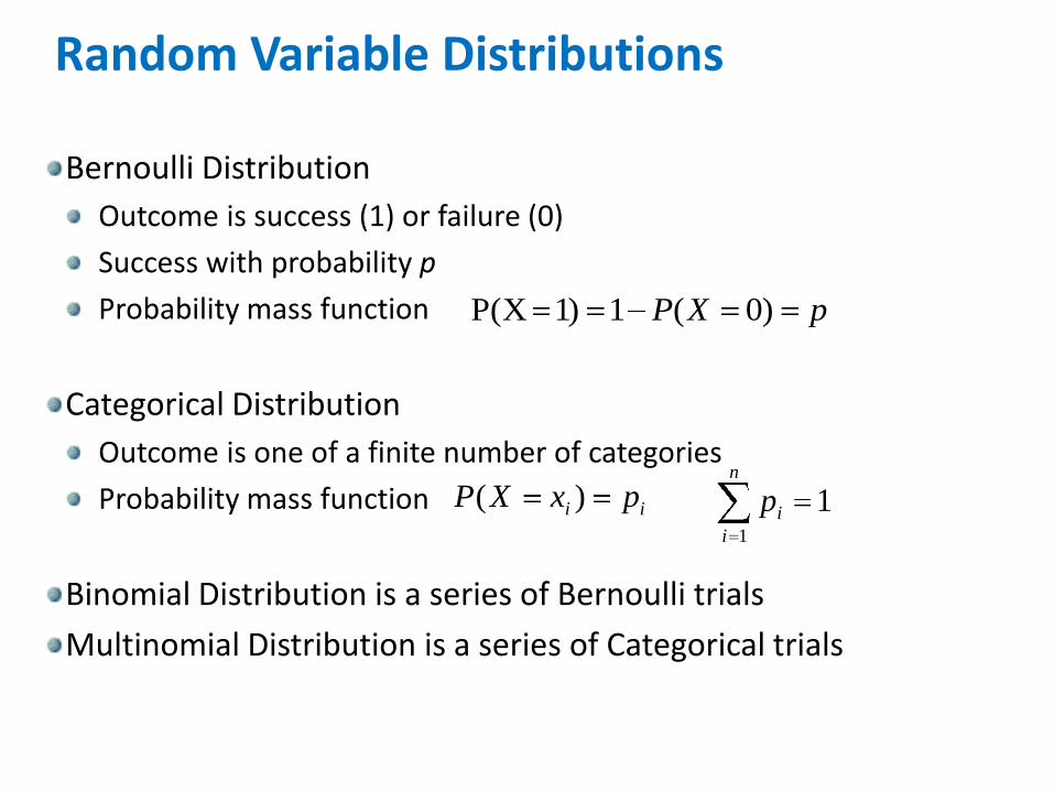
Bernoulli Distribution

Outcome is success (1) or failure (0)

Success with probability p

Probability mass function

Categorical Distribution

Outcome is one of a finite number of categories

Probability mass function

Binomial Distribution is a series of Bernoulli trials

Multinomial Distribution is a series of Categorical trials

Random Variable Distributions

pXP )0(1)1P(X

ii pxXP )( 11

n

i

ip

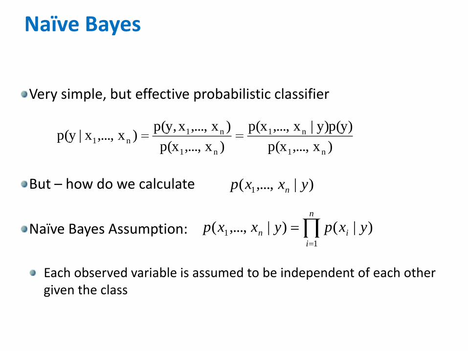
Very simple, but effective probabilistic classifier

But – how do we calculate

Naïve Bayes Assumption:

Each observed variable is assumed to be independent of each other given the class

Naïve Bayes

)x,...,p(x

y)p(y)|x,...,p(x

)x,...,p(x

)x,...,xp(y,)x,...,x|p(y

n1

n1

n1

n1n1

n

i

in yxpyxxp1

1 )|()|,...,(

)|,...,( 1 yxxp n

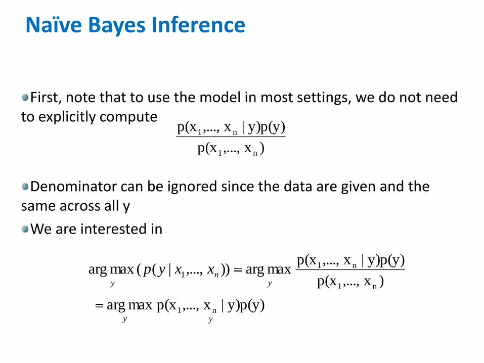
First, note that to use the model in most settings, we do not need to explicitly compute

Denominator can be ignored since the data are given and the same across all y

We are interested in

Naïve Bayes Inference

)x,...,p(x

y)p(y)|x,...,p(x

n1

n1

)x,...,p(x

y)p(y)|x,...,p(xmaxarg)),...,|((maxarg

n1

n11

yn

y

xxyp

yy

y)p(y)|x,...,p(xmaxarg n1

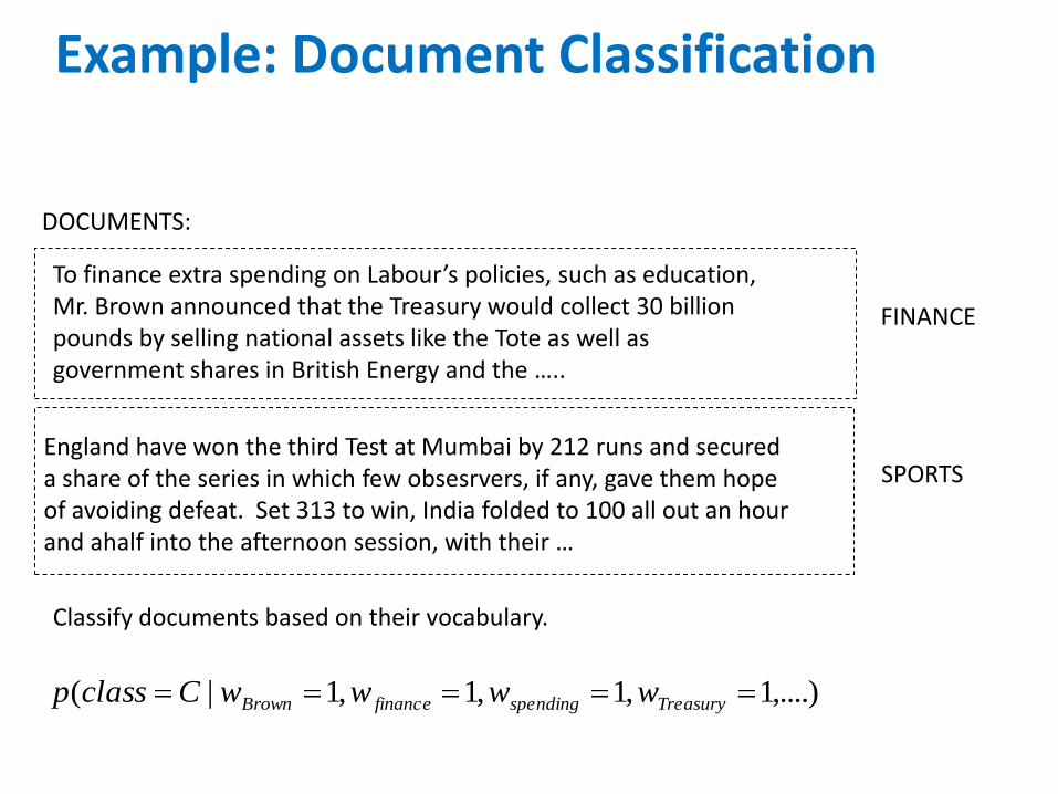
Example: Document Classification

To finance extra spending on Labour’s policies, such as education,Mr. Brown announced that the Treasury would collect 30 billionpounds by selling national assets like the Tote as well asgovernment shares in British Energy and the …..

DOCUMENTS:

England have won the third Test at Mumbai by 212 runs and secureda share of the series in which few obsesrvers, if any, gave them hopeof avoiding defeat. Set 313 to win, India folded to 100 all out an hourand ahalf into the afternoon session, with their …

Classify documents based on their vocabulary.

,....)1,1,1,1|( TreasuryspendingfinanceBrown wwwwCclassp

FINANCE

SPORTS

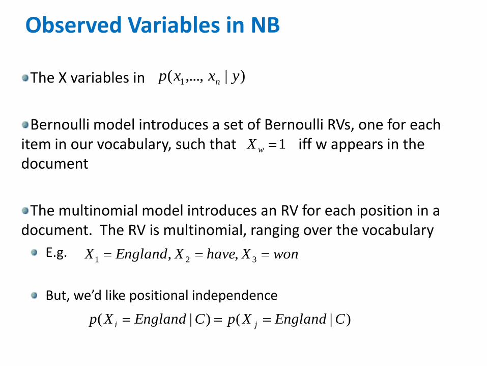
The X variables in

Bernoulli model introduces a set of Bernoulli RVs, one for each item in our vocabulary, such that iff w appears in the document

The multinomial model introduces an RV for each position in a document. The RV is multinomial, ranging over the vocabulary

E.g.

But, we’d like positional independence

Observed Variables in NB

)|,...,( 1 yxxp n

1wX

wonXhaveXEnglandX 321 ,,

)|()|( CEnglandXpCEnglandXp ji

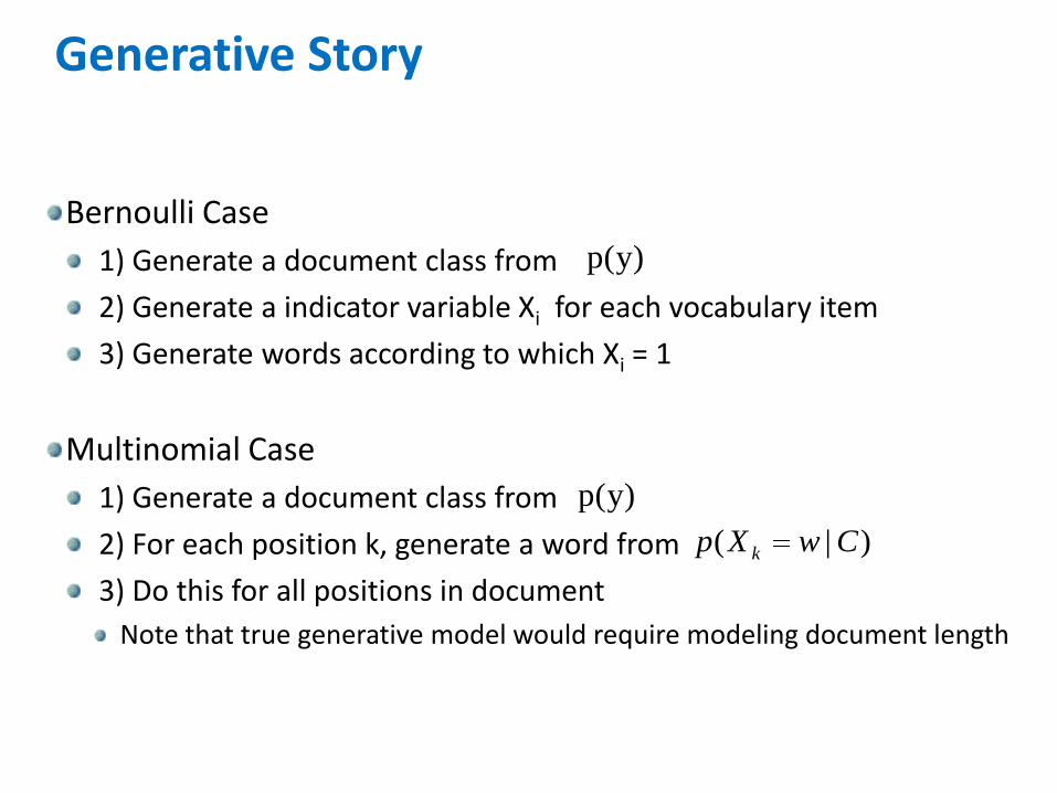
Bernoulli Case

1) Generate a document class from

2) Generate a indicator variable Xi for each vocabulary item

3) Generate words according to which Xi = 1

Multinomial Case

1) Generate a document class from

2) For each position k, generate a word from

3) Do this for all positions in document

Note that true generative model would require modeling document length

Generative Story

p(y)

p(y)

)|( CwXp k

Maximum likelihood estimation

We need to find estimates for

And for class conditional posteriors

That MAXIMIZE the likelihood

Estimation

),()|( )(

1

)( in

i

i yxpDp

n

k

kkkn

k

n

k

kkkk

n ypyxpyxpyxpDp1

)()()(

1 1

)()()()(

:1 )(log)|(log),(log),(log)|(log

)(yp

)|( yxp i

Bernoulli ML estimate

Multinomial ML estimate

Class prior ML estimate

Estimation Cont.

y class of documents across occurs x timesof #),('

in occursy that x class of docs of #),(

yxc

yxc

)(

),()|(

yc

yxcyxp i

i

j

j

ii

yxc

yxcyxp

),('

),(')|(

'

)'(

)()(

y

yc

ycyp

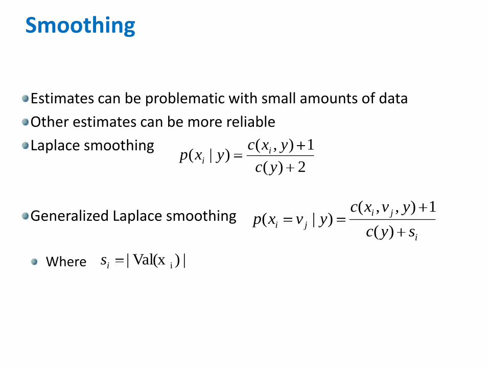
Estimates can be problematic with small amounts of data

Other estimates can be more reliable

Laplace smoothing

Generalized Laplace smoothing

Where

Smoothing

2)(

1),()|(

yc

yxcyxp i

i

i

ji

jisyc

yvxcyvxp

)(

1),,()|(

|)Val(x| iis

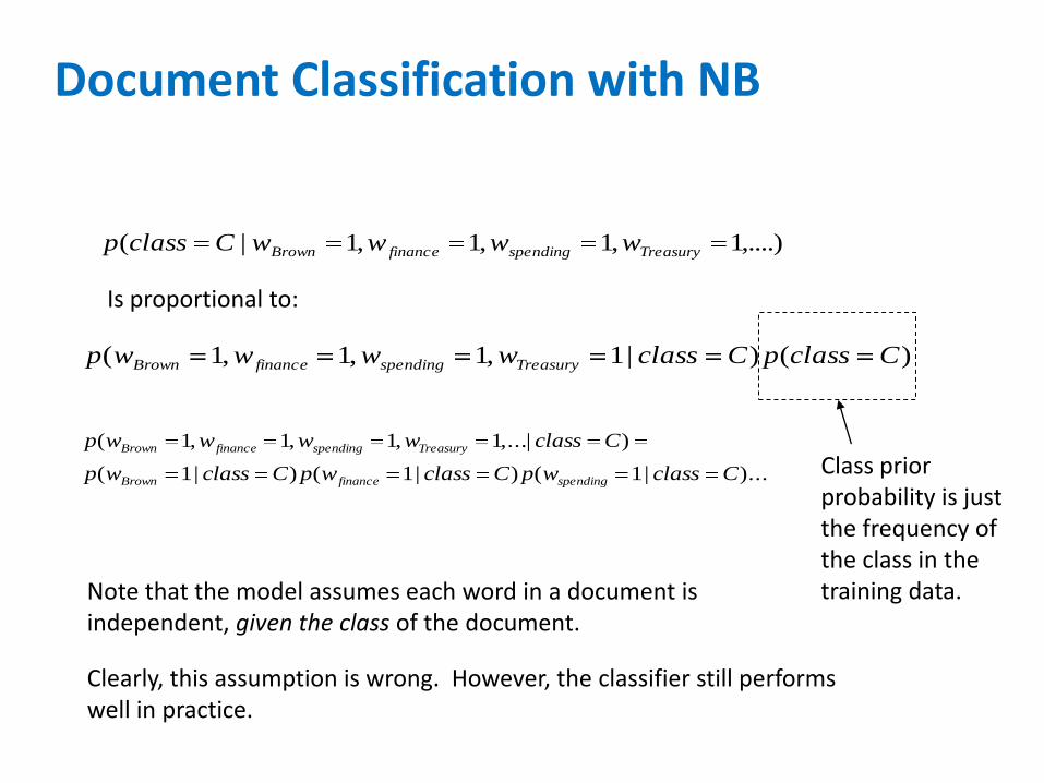
Document Classification with NB

)...|1()|1()|1(

)|,...1,1,1,1(

CclasswpCclasswpCclasswp

Cclasswwwwp

spendingfinanceBrown

TreasuryspendingfinanceBrown

,....)1,1,1,1|( TreasuryspendingfinanceBrown wwwwCclassp

Is proportional to:

)()|1,1,1,1( CclasspCclasswwwwp TreasuryspendingfinanceBrown

Class prior probability is just the frequency of the class in the training data. Note that the model assumes each word in a document is

independent, given the class of the document.

Clearly, this assumption is wrong. However, the classifier still performswell in practice.

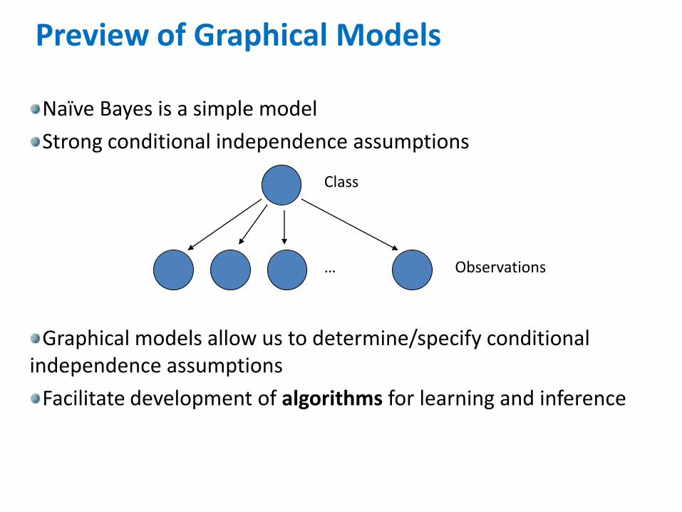
Naïve Bayes is a simple model

Strong conditional independence assumptions

Graphical models allow us to determine/specify conditional independence assumptions

Facilitate development of algorithms for learning and inference

Preview of Graphical Models

…

Class

Observations

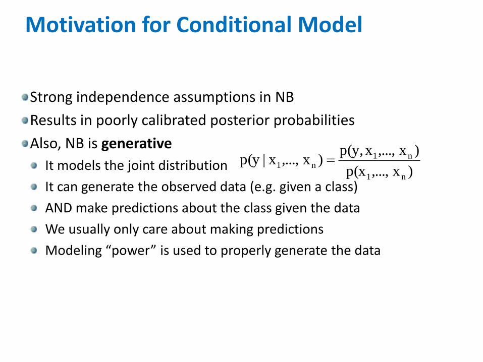
Strong independence assumptions in NB

Results in poorly calibrated posterior probabilities

Also, NB is generative

It models the joint distribution

It can generate the observed data (e.g. given a class)

AND make predictions about the class given the data

We usually only care about making predictions

Modeling “power” is used to properly generate the data

Motivation for Conditional Model

)x,...,p(x

)x,...,xp(y,)x,...,x|p(y

n1

n1n1

Instead of modeling joint distribution

Model only conditional directly

This means we can’t generate the data

Model is weaker

BUT – training it means we need not worry about independence or lack thereof among the observed variables

A Conditional Model

),,...,(1

)x,...,x|p(y 1n1 yxxFZ

n

…

Class

Observations

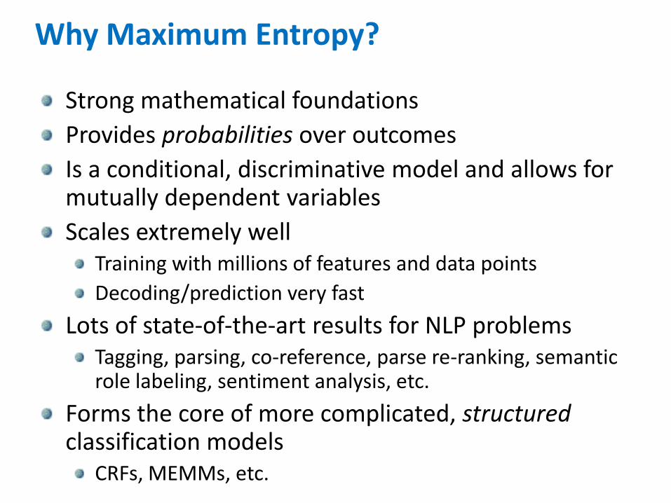
Why Maximum Entropy?

Strong mathematical foundations

Provides probabilities over outcomes

Is a conditional, discriminative model and allows for mutually dependent variables

Scales extremely wellTraining with millions of features and data points

Decoding/prediction very fast

Lots of state-of-the-art results for NLP problemsTagging, parsing, co-reference, parse re-ranking, semantic role labeling, sentiment analysis, etc.

Forms the core of more complicated, structuredclassification models

CRFs, MEMMs, etc.

9/15/2010 19

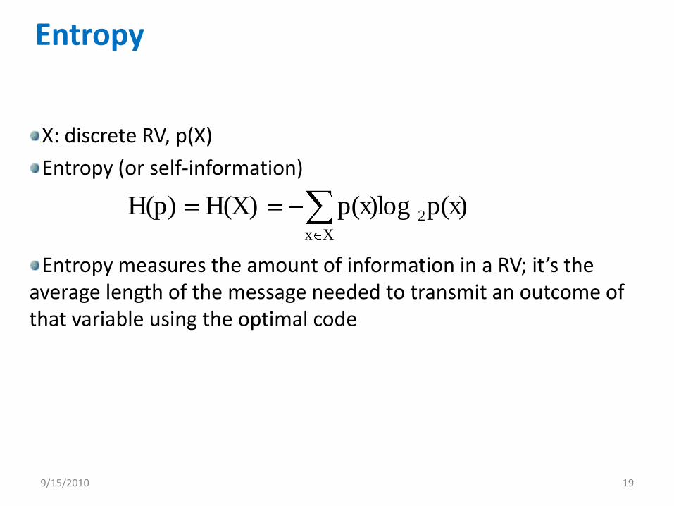
X: discrete RV, p(X)

Entropy (or self-information)

Entropy measures the amount of information in a RV; it’s the average length of the message needed to transmit an outcome of that variable using the optimal code

Entropy

p(x)p(x)logH(X)H(p)Xx

2

9/15/2010 20

Entropy (cont)

p(x)

1log E

p(x)

1p(x)log

p(x)p(x)logH(X)

2

Xx

2

Xx

2

1p(X)0H(X)

0H(X) i.e when the value of Xis determinate, hence providing no new information

9/15/2010 21

The joint entropy of 2 RV X,Y is the amount of the information needed on average to specify both their values

Joint Entropy

Xx y

2 Y)p(X,y)logp(x,Y)H(X,Y

9/15/2010 22

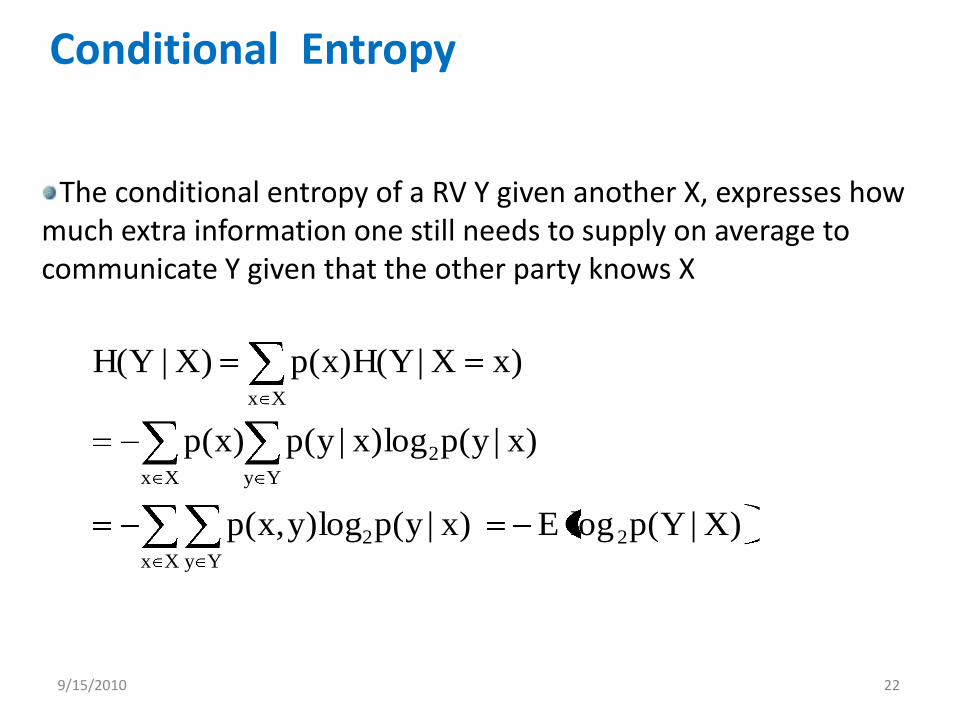
The conditional entropy of a RV Y given another X, expresses how much extra information one still needs to supply on average to communicate Y given that the other party knows X

Conditional Entropy

X)|p(YlogE x)|p(yy)logp(x,

x)|p(yx)log|p(yp(x)

x)X|p(x)H(YX)|H(Y

2

Xx Yy

2

Xx Yy

2

Xx

9/15/2010 23

Chain Rule

X)|H(YH(X) Y)H(X,

),...XX|H(X....)X|H(X)H(X)X...,H(X 1n1n121n1,

9/15/2010 24

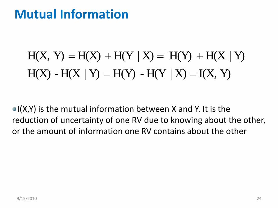
I(X,Y) is the mutual information between X and Y. It is the reduction of uncertainty of one RV due to knowing about the other, or the amount of information one RV contains about the other

Mutual Information

Y)I(X, X)|H(Y -H(Y) Y)|H(X-H(X)

Y)|H(XH(Y) X)|H(YH(X) Y)H(X,

9/15/2010 25

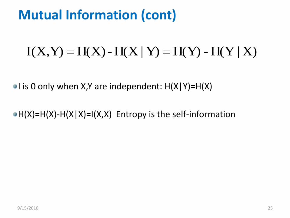
I is 0 only when X,Y are independent: H(X|Y)=H(X)

H(X)=H(X)-H(X|X)=I(X,X) Entropy is the self-information

Mutual Information (cont)

X)|H(Y -H(Y) Y)|H(X-H(X) Y)I(X,

9/15/2010 26

Entropy is measure of uncertainty. The more we know about something the lower the entropy.

If a language model captures more of the structure of the language, then the entropy should be lower.

We can use entropy as a measure of the quality of our models

Entropy and Linguistics

9/15/2010 27

H: entropy of language; we don’t know p(X); so..?

Suppose our model of the language is q(X)

How good estimate of p(X) is q(X)?

Entropy and Linguistics

p(x)p(x)logH(X)H(p)Xx

2

9/15/2010 28

Relative entropy or KL (Kullback-Leibler) divergence

Entropy and LinguisticsKullback-Leibler Divergence

q(X)

p(X)logE

q(x)

p(x)p(x)log q) ||D(p

p

Xx

9/15/2010 29

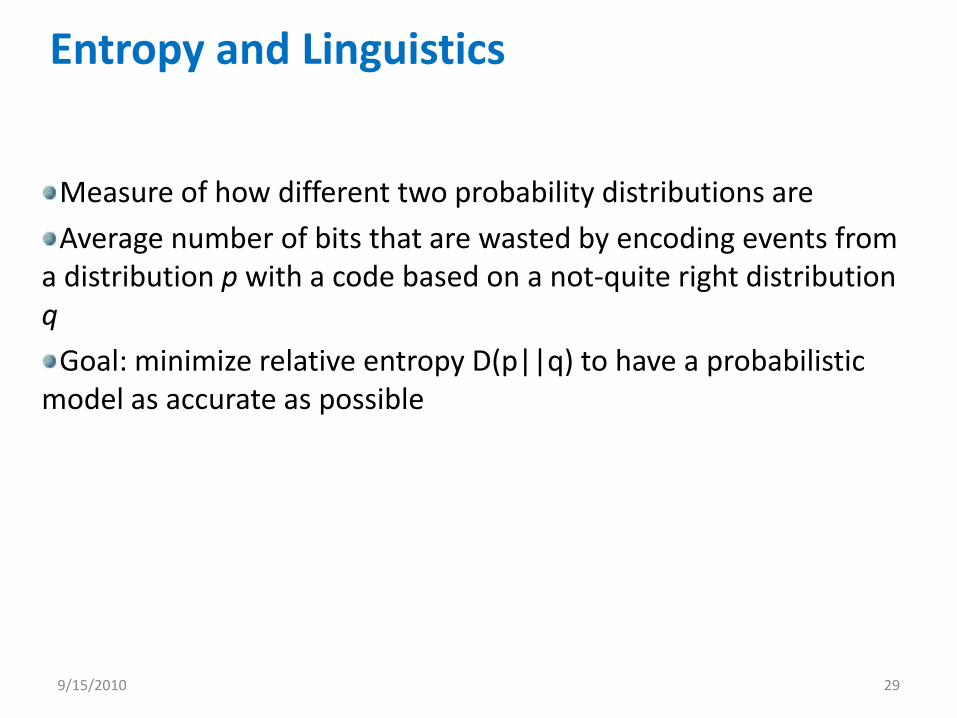
Measure of how different two probability distributions are

Average number of bits that are wasted by encoding events from a distribution p with a code based on a not-quite right distribution q

Goal: minimize relative entropy D(p||q) to have a probabilistic model as accurate as possible

Entropy and Linguistics

Maximum Entropy: Intuition

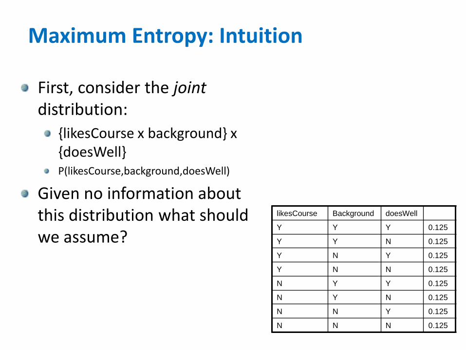
First, consider the jointdistribution:

{likesCourse x background} x {doesWell}P(likesCourse,background,doesWell)

Given no information about this distribution what should we assume?

likesCourse Background doesWell

Y Y Y 0.125

Y Y N 0.125

Y N Y 0.125

Y N N 0.125

N Y Y 0.125

N Y N 0.125

N N Y 0.125

N N N 0.125

Maximum Entropy: Intuition

What if we examine data and see that Jane does well and likes the course 70% of the time?

likesCourse Background doesWell

Y Y Y 0.35

Y Y N 0.05

Y N Y 0.35

Y N N 0.05

N Y Y 0.05

N Y N 0.05

N N Y 0.05

N N N 0.05

What is Entropy?

Measures uncertainty in a distribution

For a fixed value of x, we have:

Conditional entropy:

Goal: select a distribution p from a set of allowed distributions that maximizes H(Y|X)

yx

yxpyxpYXH,

),(log),(),(

yx

xypxypxpXYH,

)|(log)|()(~)|(

)|(maxarg* XYHp p

y

xypxypxXYH )|(log)|()|(

Maximum Entropy Model

Such a model can be shown to have the following form:

z k

kk

k

kk

zxf

yxf

xyp)),(exp(

)),(exp(

)|(

Where the are the model parameters and the are the featuresof the model.

k kf

Constraints: Empirical Expectations

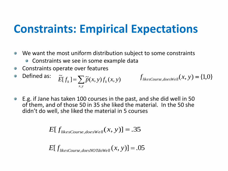
We want the most uniform distribution subject to some constraintsConstraints we see in some example data

Constraints operate over featuresDefined as:

E.g. if Jane has taken 100 courses in the past, and she did well in 50 of them, and of those 50 in 35 she liked the material. In the 50 she didn’t do well, she liked the material in 5 courses

05.)],([ , yxfE elldoesNOTdoWelikesCours

}0,1{),(, yxf doesWellelikesCours

35.)],([ , yxfE doesWellelikesCours

yx

kk yxfyxpfE,

),(),(~][~

Model Expectations

Feature expectations, according to a model are defined:

Goal:

yx

k yxfxypxpfE,

),()|()(~][

)|(maxarg* XYHp p

][~

][ kk fEfEsuch that

i.e.yx

k

yx

k yxfyxpyxfxypxp,,

),(),(),()|()(~

for all k

Lagrange Multipliers (* Optional slide)

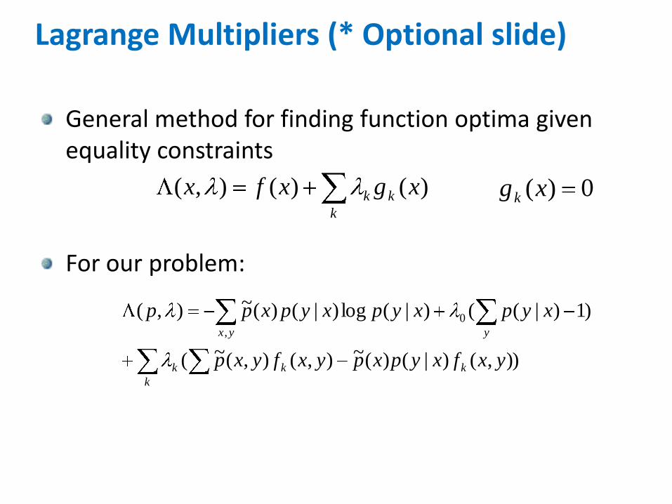
General method for finding function optima given equality constraints

For our problem:

k

kk xgxfx )()(),(

)),()|()(~),(),(~(

)1)|(()|(log)|()(~),( 0

,

yxfxypxpyxfyxp

xypxypxypxpp

kk

k

k

yyx

0)(xgk

Derivation of Max Entropy (* Optional Slide)

)),()(~())|(log1)((~

)|(

),(0 yxfxpxypxp

xyp

x

k

kk

0)),()(~())|(log)(~)(~0 yxfxpxypxpxp

k

kk

Set this to zero and solve:

1)(~),()|(log 0

xpyxfxyp

k

kk

)1)(~exp()),(exp()|( 0

xpyxfxyp

k

kk

We know that is the multiplier over the constraint that requires the distribution sum to 1, therefore it corresponds to a normalizing constant:

0

z k

kk

k

kk

zxf

yxf

xyp)),(exp(

)),(exp(

)|(

Maximum Likelihood Training

Given a set of training data, we would like to find a set of model parameters that best explain the data – a set of parameters that make the data most likely:Example:

You observe an (unfair) coin flipped 100 times. It turns up heads 60 times. The possible ‘parameters’ for the coin are: p(HEADS) = 1/3, p(HEADS) = ½, p(HEADS)= 2/3Which coin was most likely used?

For prediction tasks using a conditional probability model (not just MaxEnt), this is formulated as:

||

1

)()( )|(log)(maxargD

i

ii

D xyppL

||

1

)()( )|(logD

i

ii xyp

Maximum Likelihood

||

1)()(

)()(

),(exp

),(exp

logD

i

z k

ii

kk

k

ii

kk

yxf

yxf

This function turns out to be convex with a single global maximum. How do we maximize such a function?

||

1

)()(||

1

)()( ),(explog),(D

i z k

ii

kk

D

i k

ii

kk zxfyxf

||

1

)()( )|(log)(maxargD

i

ii

D xyppL

||

1

)()( )|(logD

i

ii xyp

Gradient of the Log-Likelihood

We take the partial derivative with respect to each parameter, k

||

1

'

||

1

)()(

)',(exp

),(exp),(

),()( D

i z

z k

kk

k

kkkD

i

ii

k

k

D

zxf

zxfzxf

yxfpL

||

1

||

1

),()|(),(D

i z

k

D

i

k zxfxzpyxf

0][][~

kk fEfE Gradient is just the difference in featureexpectations. But, expectation for a particular feature is dependent on ALLthe other parameters. No closed form!

And set to 0

Contrast with Naïve Bayes

No closed form

Computationally Expensive

The expectation for each feature requires knowing the expectations of all the other features

We must determine the best parameter values “jointly” over all features

This is what allows MaxEnt to gracefully handle features that are not independent and “do the right thing”

If two features are completely dependent, they will have the same learned parameter values

MaxEnt Estimation

Parameter Estimation

Use iterative scaling methodsAdjust one parameter with all others fixed

Apply any non-linear numerical optimization methodMethods divided into:

First order methods:Move in direction of steepest ascentDirection a function of steepest direction + last directionConjugate gradient, Newton’s method

Second order methods:Consider the curvature of the function – it’s second derivative – Hessian matrixSmarter about picking good directionsHessian is too big, methods use an approximate version

MAP Inference

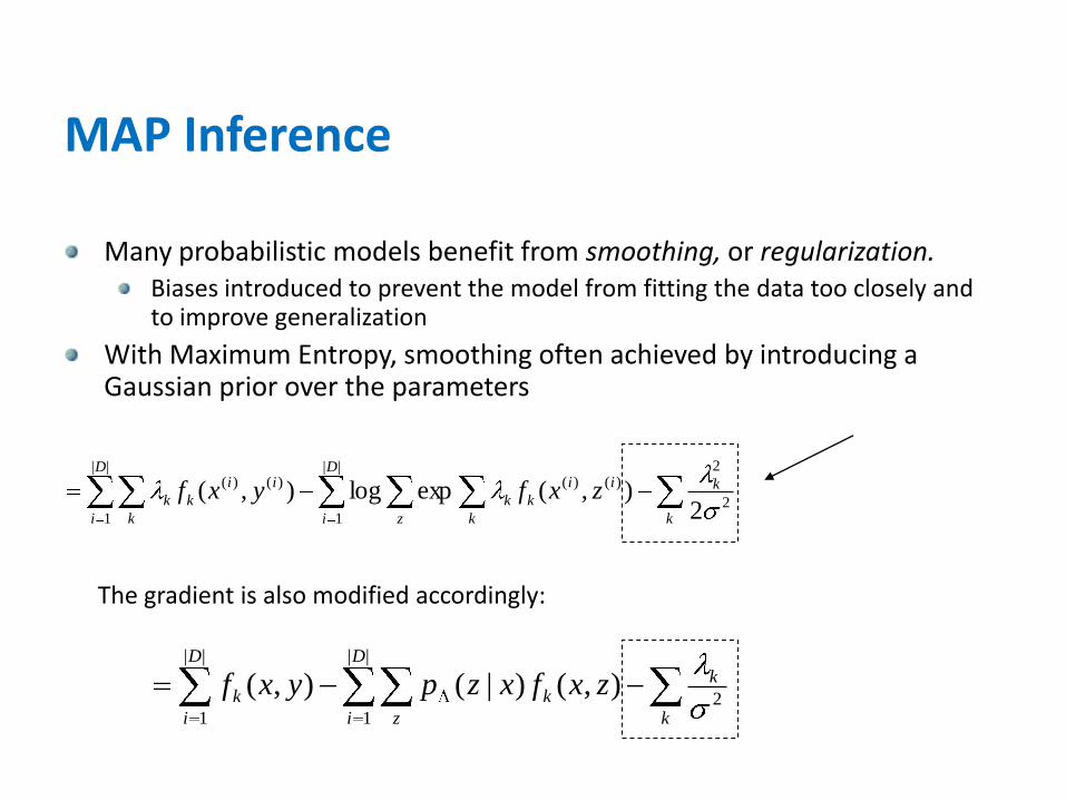
Many probabilistic models benefit from smoothing, or regularization.Biases introduced to prevent the model from fitting the data too closely and to improve generalization

With Maximum Entropy, smoothing often achieved by introducing a Gaussian prior over the parameters

The gradient is also modified accordingly:

k

k

D

i z k

ii

kk

D

i k

ii

kk zxfyxf2

2||

1

)()(||

1

)()(

2),(explog),(

k

k

D

i z

k

D

i

k zxfxzpyxf2

||

1

||

1

),()|(),(

Averaged Perceptron

Repeatedly classify examples in training data

When mistakes are made with current parameters

Update parameter values

Repeat until convergence

Stochastic Gradient Descent

Take a small sample of the training data

Compute the log-likelihood gradient for just that sample

Update parameters based on the gradient

Repeat until convergence

Other Ways to Estimate Parameters

Input: Training examples

Initialization:

For

Calculate

If then

Output

Predict using:

Averaged Perceptron

)},(),...,,{( )()()1()1( nn yxyxD

]0...0[

niTt ,...,1,,...,1

)',(),( )()()()( ii

k

ii

kkk yxfyxf)()(' ii yy

k

i

kky

i yxfy ),(maxarg' )()(

),...,(),(maxarg 1)( Tn

kk

k

i

ky

avgyxf

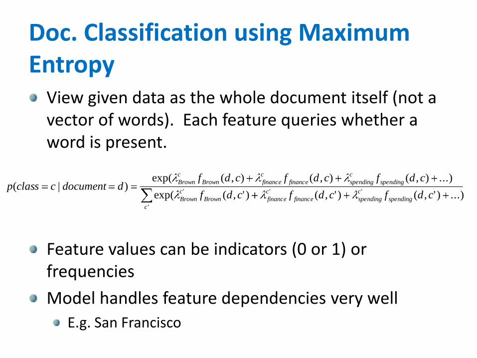
Doc. Classification using Maximum Entropy

View given data as the whole document itself (not a vector of words). Each feature queries whether a word is present.

Feature values can be indicators (0 or 1) or frequencies

Model handles feature dependencies very well

E.g. San Francisco

'

''' ...))',()',()',(exp(

...)),(),(),(exp()|(

c

spending

c

spendingfinance

c

financeBrown

c

Brown

spending

c

spendingfinance

c

financeBrown

c

Brown

cdfcdfcdf

cdfcdfcdfddocumentcclassp

Graphical Models

Naïve Bayes

Maximum Entropy

…

Class

Observations

…

Class

Observations

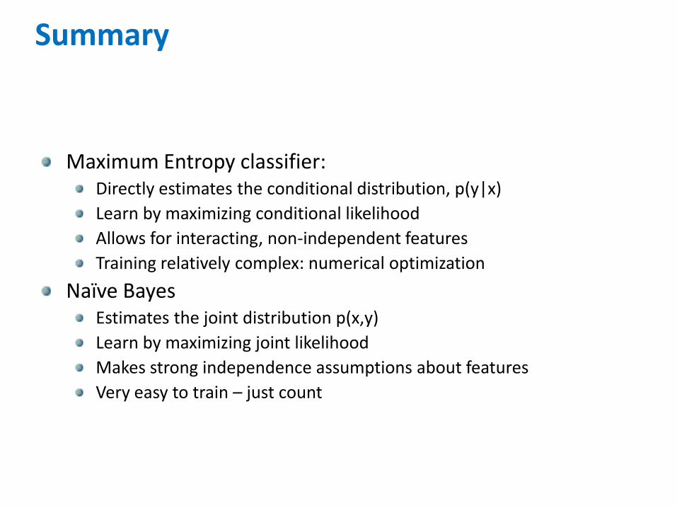
Summary

Maximum Entropy classifier:Directly estimates the conditional distribution, p(y|x)

Learn by maximizing conditional likelihood

Allows for interacting, non-independent features

Training relatively complex: numerical optimization

Naïve BayesEstimates the joint distribution p(x,y)

Learn by maximizing joint likelihood

Makes strong independence assumptions about features

Very easy to train – just count