N91- lTS - NASA

N91- lTS Radar Signal Categorization using a Neural Network

James A. Anderson

Department of Cognitive and Linguistic Sciences

Box 1978

Brown University, Providence, RI 02912

and

Michael T. Gately, P. Andrew Penz, and Dean R. Collins

Central Research Laboratories, Texas Instruments

Dallas, Texas 75265

Accepted for Publication, IEEE ProceedingsTo appear, August, T990

(c) IEEE

This research was initially supported by Texas Instruments, the Office of NavalResearch (Contract N00014-86-K-0600 to J.A.) and the National Science Foundation

(Grant BNS-85-18675 to J.A.). Currently, this research is supported by the Avionics

Laboratory, Wright Research and Development Center, Aeronautical Systems Division[Contract F33615-87-C1454].

107

Radar Signal Categorization Using a Neural Network

Abstract

Neural networks were used to analyze a complex simulated radarenvironment which contains noisy radar pulses generated by manydifferent emitters. The neural network used is an energy

minimizing network (the BSB model) which forms energy minima --attractors in the network dynamical system -- based on learned

input data. The system first determines how many emitters arepresent (the delnterleaving problem). Pulses from individualsimulated emitters give rise to separate stable attractors in thenetwork. Once individual emitters are characterized, it is

possible to make tentative identifications of them based on theirobserved parameters. As a test of this idea, a neural networkwas used to form a small data base that potentially could makeemitter identifications.

We have used neural networks to cluster, characterize and identify radar signals

from different emitters. The approach assumes the ability to monitor a region of themicrowave spectrum and to detect and measure properties of received radar pulses.The microwave environment is assumed to be complex, so there are pulses from a number

of different emitters present, and pulses from the same emitter are noisy or their

properties are not measured with great accuracy.

For several practical appllcatlons, it is important to be able to tell quickly,

first, how many emitters are present and, second, what their properties are. Inother words time average prototypes must be derived from time dependent data without

a tutor. Finally the system must tentatively identify the prototypes as members ofpreviously seen classes of emitter.

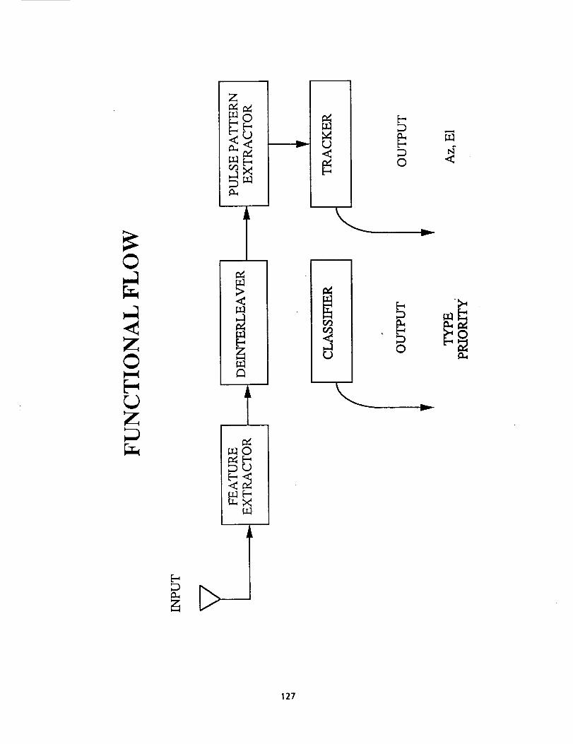
Stages of Processing. We accomplish this task in several stages. Figure Ishows a _lo-_k diagram of the resulting system, which contains several neuralnetworks. The system as a whole is referred to as the Adaptive Network Sensor

Processor (ANSP).

Figure I About Here

o

In the block diagram given in Figure i, the first block is a feature extractor.

We start by assuming a microwave radar receiver of some sophistication at the inputto the system. This receiver is capable of processing each pulse into featurevalues, i.e. azimuth, elevation, signal to noise ratio (normalized intensity),

frequency, and pulse width. This data is then listed in a _ buffer and taggedwith time of arrival of the pulse. In a complex radar envir_, hundreds or

thousands of pulses can arrive in fractions of seconds, so there is no lack of data.

The problem, as in many data rich environments, is making sense of it.

108

The second block in Figure 1 is the deinterleaver which clusters incoming radar

pulses into groups, each group formed by pulses from a single emitter. A number of

pulses are observed, and a neural network computes, off line, how many emitters arepresent, based on the sample, and estimates their properties. That is, it solves theso-called deinterleaving problem by identifying pulses as being produced by a

particular emitter. This block also produces and passes forward measures of the eachcluster's azimuth, elevation, SNR, frequency and pulse width.

The third block, the pulse pattern extractor, uses the deinterleaved information

to compute the pulse repetition pattern of an emitter by using the times of arrivalfor the pulses that are contained in a given cluster. This information will be used

for emitter classification.

The fourth block, the tracker, acts as a long term memory for the clusters found

in the second block, storing the average azimuth, elevation, SNR, frequency, and

pulse width. Since the diagram in Figure 1 is organized via initial computationalfunctionality, the tracking module follows the deinterleaver so as to store its

outputs. In an operationally organized diagram, the tracker is the first block toreceive pulse data from the feature extractor. It must identify most of the pulsesin real time as previously learned by the deinterieaver module and only pass a smallnumber of unknown pulses back to the deinterleaver module for further learning. The

tracker also updates the cluster averages. Their properties can change with timebecause of emitter or receiver motion, for example.

The fourth and fifth blocks, the tracker and the classifier operate as a unit to

classify the observed emitters, based on information stored in a data base of emitter

types. Intrinsic emitter properties stored in these blocks are frequency, pulsewidth and pulse repetition pattern.

The most important question for the ANSP to answer is what the emitters might beand what can they do. That is, "who is looking at me, should I be concerned, and

should I (or can I) do something about it?"

Emitter Clustering. Most of the initial theoretical and simulation effort inthis project has been focused on the deinterleaving problem. This is because theANSP is being asked to form a conception of the emitter environment from the dataitself. A teacher does not exist for most interesting situations.

In the simplest case, each emitter emits with constant properties, i.e. nonoise is present. Then, determining how many emitters were present would be trivial:

simply count the number of unique pulses via a look up table. Unfortunately, data isoften moderately noisy because of receiver, environmental and emitter variability,

and, sometimes, because of the frequent change of one or another emitter property atthe emitter. Therefore, simple identity checks will not work. It is these later

cases which this paper will address.

Many neural networks are supervised algorithms, that is, they are trained by

seeing correctly classified examples of training data and, when new data is presentedwill identify it according to their past experience. Emitter identification does notfall into this category because the correct answers are not known ahead of time.

That, after all, is the purpose of this system. The baslc problem of a

self-organizlng clustering system has many historical precedents in cognitivescience. For example, William James, in a quotation well known to developmental

psychologists, wrote around 1890,

109

..the numerous inpouring currents of the baby bring to his

consciousness ... one big blooming buzzing Confusion. That

Confusion is the baby's universe; and the universe of all of usis still to a great extent such a Confusion, potentiallyresolvable, and demanding to be resolved, but not yet actually

resolved into parts.

William James (1890, p.29)

We nov know that the new born baby is a very competent organism, and the

outlines of adult perceptual preprocesslng are already in place. The baby is

designed to hear human speech in the appropriate way and to see a world llke ours:that is, a baby is tuned to the environment in which he will live. The same is trueof the ANSP, which must process pulses which will have feature values that fall

within certain parameter ranges. That is, an effective feature analysis has been

done for us by the receiver designer, and we do not have to organize a system fromzero. This means that we can use a less general approach than we might have to in a

less constrained problem. The result of both evolution and good engineering designis to build so much structure into the system that a problem, very difficult in its

general form, becomes quite tractable.

At this point, neural networks are familiar to many. Introductions are

available, for example, McClelland and Rumelhart, 1986; Rumelhart and McClelland,

1986; Hinton and Anderson, 1989; Anderson and Rosenfeld, 1988.

The Linear Assoclator. Let us begin our discussion of the network we shall use

for t-__ problem with the 'outer product' associator, also called the 'linear

assoclator,' as a starting point. (Kohonen, 1972, 1977, 1984; Anderson, 1972). Weassume a single computing unit, a simple model neuron, acts as a linear summer of its

inputs. There are many such computing units. The set of activities of a group ofunits is the system state vector. Our notation has matrices represented by capitalletters (A), vectors by lower case letters (f,g), and the elements of vectors as f(i)

or g(j). A vector from a set of vectors is subscripted, for example, fl' f2 ....

The ith unit in a set of units will display activity g(i) when a pattern f(J) is

presented t-6 its inputs, according to the rule,

g(1) = E A(i,j) f(j).J

where A(i,j) are the connections between the ith unit in an output set of units and

the jth unit in an input set. We can then c-'anwrite the output pattern, g, as the

matrix-_ultiplication

g=Af.

During learning, the connection strengths are modified according to a

generalized Hebb rule, that is, the change in an element of A, &_(i,J), is given by

110

8A(i,j) m f(j) g(i),k k

where f and g are vectors associated with the kth learning example.k k

Then we can write the matrix A as a sum of outer products,

n T

A=nZ gfk=l k k

where _ is a learning constant.

Prototype Formation The linear model forms prototypes as part of the storage

process, a property we will draw on. Suppose a category contains many similar itemsassociated with the same response. Consider a set of correlated vectors, {fk}, with

mean p.

f =p+d •k k

The final connectivity matrix will be

n T

A=r#gfk=l k

T n T

rg(np + E d )k=l k

If the sum of the dk is small, the connectivity matrix is approximated by

T

A = _n g p .

The system behaves as if it had repeatedly learned only one pattern, p, and respondsbest to it, even though p, in fact, may never have been learned.

Concept forming systems. Knapp and Anderson (1984) applied this model directlyto the formation of simple psychological 'concepts' formed of nine randomly placed

dots. A 'concept' in cognitive science describes the common and important situationwhere a number of different objects are classed together by some rule or similarity

relationship. Much of the power of language, for example, arises from the ability to

see that physically different objects are really 'the same' and can be named andresponded to in a similar fashion, for example, tables or lions. A great deal of

experimentation and theory in cognitive science concerns itself with conceptformation and use.

There are two related but distinct ways of explaining simple concepts in neuralnetwork models. First, there are prototype forming systems, which often involve

taking a kind of average during the act of storage, and, second, there are modelswhich explain concepts as related to attractors in a dynamical system. In the radarANSP system to be described we use both ideas: we want to construct a system where

111

the average of a category becomes the attractor in a dynamical system, and anattractor and its surrounding basin represent an individual emitter. (For a furtherdiscussion of concept formation in simple neural networks, see Knapp and Anderson,

1984_ Anderson, 1983, and Anderson and Murphy, 1986).

Error Correction. By using an error correcting technique, the Widrow-Hoffproce_ we can force the simple associative system to give us more accurateassociations. Let us assume we are working with an autoassociative system. Suppose

information is represented by associated vectors fl * fl, fo * f_ .... A vector,fk' is selected at random. Then the matrix, A, is incremented a_cording to the rule

T

6A = _ (f - Af) fk k k

where _A is the change in the matrix A. In the radar application, there is no'correct answer' in the general sense of a supervised algorithm. However every input

pattern can be its own 'teacher' in the error correction algorithm in that the

network will try to better reconstruct that particular input pattern. The goal oflearning a set of stimuli {f} is to have the system behave as

Af=f

k k

The error correcting learning rule will approximate this result with a least meansquares approximation, hence the alternative name for the Widrow-Hoff rule: the LMS

(least mean squares) algorithm. The autoassoclative system combined with error

correction, when working perfectly, is forcing the system to develop a particular setof eigenvectors with eigenvalue 1.

The eigenvectors of the connection matrix are also of

Hebblan learning is used in an autoassoclatlve system.product assoclator has the form

interest when simpleThen, the simple outer

T

AA=nf fk k

There is now an obvious connection between the elgenvectors of the resulting

outer product connectivity matrix and the principal components of statistics, becausethe form of this matrix is the covarlance matrix. In fact, there is growing evidence

that many neural networks are doing something llke principal component analyis.(See, for example, Baldi and Hornik, 1989 and Cottrell, Munro and Zipser, 1988).

BSB: A.Dynamical System. We shall use for radar clustering a non-linear modelthat t-_es- the basic linear assoclator, uses error correction to construct the

connection matrix, and uses units containing a simple limiting non-linearlty.Consider an autoassoclative feedback system, where the vector output from the matrixis fed back into the input. Because feedback systems can become unstable, we

incorporate a simple limiting non-linearity to prevent unit activity from getting toolarge or too small. Let f[i] be the current state vector describing the system.

f[0] is the vector at step 0. At the i+Ist step, f[i+l], the next state vector, isgiven by the Iteratlve equation,

112

f[i+l] = LIMIT [ _A f[i] + y f[i] + 8 f[O] ].

We stabilize the system by bounding the element activities within limits.

The first term, _Af[i], passes the current system state through the matrix andadds information reconstructed from the autoassoclatlve cross connections. The

second term, vf[i], causes the current state to decay slightly. This term has the

qualitative effect of causing errors to eventually decay to zero as long as y is

less than 1. The third term, 6f[O], can keep the initial information constantlypresent and has the effect of limiting the flexibility of the possible states of the

dynamical system since some vector elements are strongly biased by the initial input.

Once the element values for f[i+l] are calculated, the element values are

'limited', that is, not allowed to be greater than a positive limit or less than a

negative limit. This is a particularly simple form of the sigmoidal nonlinearityassumed by most neural network model. The limiting process contains the state vectorwithin a set of limits, and we have previously called this model the 'brain state in

a box' or BSB model. (Anderson, Silverstein, Ritz, and Jones, 1977; Anderson and

Hozer, 1981) The system is in a positive feedback loop but is amplitude limited.

After many iterations, the system state becomes stable and will not change: thesepoints are attractors in the dynamical system described by the BSB equation. This

final state will be the output of the system. In the fully connected case with a

symmetric connection matrix the dynamics of the BSB system can be shown to beminimizing an energy function. The location of the attractors is controlled by thelearning algorithm. (Hopfield, 1982_ Golden, 1986). Aspects of the dynamics of this

system are related to the 'power' method of elgenvector extraction, since repeatediteration will leada to activity dominated by the eigenvectors with the largest

postive elgenvalues. The signal processing abilities of such a network occur becauseelgenvectors arising from learning uncorrelated noise will tend to have smalleigenvalues, while signal related eigenvectors will be large, will be enhanced by

feedback, and will dominate the system state after a number of iterations.

We might conjecture that a category or a concept derived from many noisyexamples would become identified with an attractor associated with a region in statespace and that all examples of the concept would map into the point attractor. Thisis the behavior we want for radar pulse clustering.

Neural Network Clustering Al_orithms. We know there will be many radar pulses,but we _ not know the detailed descriptions of each emitter invoved. We want todevelop the structure of the microwave environment, based on input information. A

number of models have been proposed for this type of task, including various

competitive learning algorithms (Rumelhart and Zipser, 1986; Carpenter and Grossberg,1987).

Each pulse is different because of noise, but there are only a small number of

emitters present relative to the number of pulses. We take the input datarepresenting each pulse and form a state vector with it. A sample of several hundredpulses are stored in a 'pulse buffer.' We take a pulse at random and learn it, using

the Widrow-Roff error correcting algorithm with a small learning constant. Sincethere is no teacher, the desired output is assumed to be the input pulse data.

Learning rules for this class of dynamical system, Rebbian learning in general,

(Hopfield, 1982) and the Widrow-Hoff rule in particular, are effective @t 'diggingholes in the energy landscape' so they fall where the vectors that are learned are.

That is, the final low energy attractor states of the dynamical system when BSB

113

dynamics are applied will tend to lie near or on stored information. Suppose welearn each pulse as it comes in, using Widrow Hoff error correction, but with a smalllearning constant. Metaphorically, we 'dig a little hole' at the location of thepulse. But each pulse is different. So, after a while, we have dug a hole for each

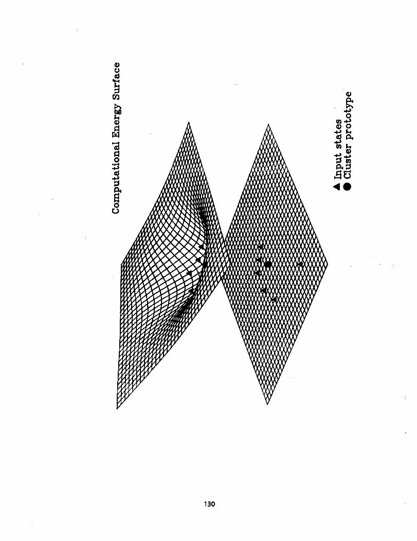
pulse, and if the state vectors _ the _ulses from a si__le emitter are not toofar apart-Tn--_tate space, we have for-_da-na'ttr-'_o_ that contains aI_-'the--puls-_t_-om a singl_'-emi-_, as well as new pulses from the same emitter. Figure 2presents a (somewhat fanciful) picture of the behavior that we hope to obtain, wheremany nearby data points combine to give a single broad network energy minimum thatcontains them all.

Figure 2 about here

We can see why this behavior will occur from an informal argument. Call theaverage emitter state vector of a particular emitter p. Then, every observed pulse,

fk' will be

f=p+d ,k k

where dk is a distortion, which will be assumed to be different for every individualpulse, that Is, different d_ are uncorrelated, and are relatively small compared top. With a small learning constant, and with the connection matrix A starting fromzero, the magnitude of the output vector, Af, will also be small after only a few

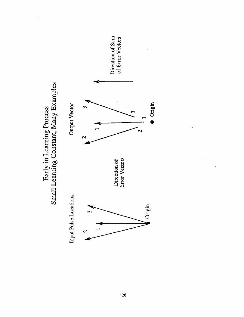
pulses are learned. This means that the error vector will point outward, toward fk'

that is, toward P+dk, as shown in Figure 3.

Figure 3 about here

Early in the learning process with a small learning constant for a particularcluster, the error vectors (input minus output) all will point toward the cluster of

input pulses. Widrow Hoff learning can be described as using a simple assoclator to

learn the error vector. Since every dk is different and uncorrelated, the errorvectors from different pulses will have the average direction of p. The matrix will

act as if it is repeatedly learning p, the average of the vectors. It is easy toshow that if the centers of different emitter clusters are spaced far apart, in

particular, if the cluster centers are orthogonal, then p will be close to aneigenvector of A. In more interesting and difficult cases, where clusters are close

together or the data is very noisy, it is necessary to resort to numerical simulationto see how well the network works in practice. As we hope to show, this technique

does work quite well.

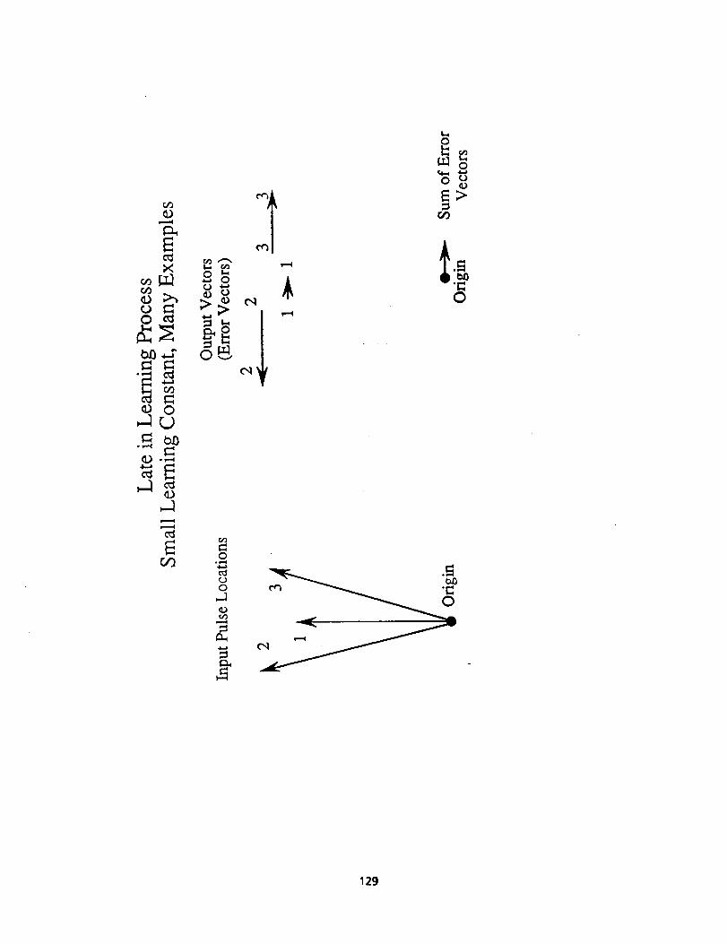
After the matrix has learned so many pulses that the input and output vectors

are of comparable magnitude, the output of the matrix when p + dk is presented willbe near p. (See Figure 4) Then,

114

p =Ap.

Over a number of learned examples,

total error = Z (P+dl - A(p+d )k k

= _(d - Ad)k k

The maximum values of the eigenvalues of A are 1 or below, the d's are uncorrelated,and this error term will average to zero.

Figure 4 about here

However, as the system learns more and more random noise, the average magnitudeof the error vector will tend to get longer and longer, as the elgenvalues of A

related to the noise become larger. Note that system learning never stops becausethere is always an error vector to be learned, which is a function of the intrinsicnoise in the system. Therefore, there is a 'senility' mechanism found in this class

of neural networks. For example, the covarlance matrix of independent, identically

distributed Gausslan noise added to each element is proportional to the identitymatrix, then every vector becomes anelgenvector wlth the same elgenvalue, and thismatrix is the matrix toward which A will evolve, if it continues to learn random

noise indefinitely. When the BSB dynamics are applied to matrices resulting fromlearning very large numbers of noisy pulses, the attractor basins become fragmented,so that the clusters break up. However, the period of stable cluster formation is

very long and it is easy to avoid cluster breakup in practice. (Anderson, 1987)

In BSB clustering the desired output is a particular stable state. Ideally, all

pulses from one emitter will be attracted to that final state. Therefore a simpleidentity check is now sufficient to check for clusters. This check is performed byresubmitting the original noisy pulses to the network that has learned them and

forming a list of the stable states that result. The llst is then compared withitself to find which pulses came from the same emitter. For example, a symbol couldbe associated with the pulses from the same final state, i.e. the pulses have beendelnterleaved or identified.

Once the emitters have been identified, the average characteristics of thefeatures describing the pulse (frequency, pulse width and pulse repetition pattern)

can be computed. These features are used to classify the emitters with respect toknown emitter types in order to 'understand' the microwave environment. A two stagesystem, which first clusters and then counts clusters is easy to implement, and,practically, allows convenient _hooks' tO use traditional digital techniques inconjunction with the neural networks.

Stimulus Coding and Representation. The fundamental represention assumption ofalmost all neural n--6tworksis that information is carried by the pattern or set of

activities of many neurons in a group of neurons. This set of activities carries the

115

meaning of whatever the nervous system is doing and these sets of activities are

represented as state vectors. The conversion of input data into a state vector, thatis, the representation of the data in the network, is the single most important

engineering problem faced in network deslgn. In our opinlon[ _hoice of-_o0d inputand output representat--fo_ is usually more important for the ultimate success of the

system than the choice of a particular network algorithm or learning rule.

We now suggest an explicit representation of the radar data. From the radarreceiver, we have a number of continuous valued features to represent: frequency,

elevation, azimuth, pulse width, and signal strength. Our approach is to codecontinuous information as locations on a topographic map, i.e. a bar graph or a

moving meter pointer. We represent each continuous parameter value by location ofblock of activation on a linear set of elements. Increase in a parameter value moves

the block of activity to the right, say, and a decrease, moves the activity to theleft. We have used a more complex topographic representation in several other

contexts, with success. (Sereno, 1989; Rossen, 1989; Viscuso, Anderson, and Spoehr,

1989).

We represent the block/bar of activity value with a block (three or four) "=",

equal, symbols placed in a region of ".," perlod, symbols. Single characters arecoded by eight bit ASCII bytes. The ASCII l's and O's are further transformed to+l's and -l's_ so that the magnitude of any feature vector is the same regardless ofthe feature value. Input vectors are therefore purely binary. On recall, if the

vector elements coding a character do not rise above a threshold size, the system isnot 'sure' of the output. Then that character is represented as the underline, " "character. Being 'not sure' can be valuable information relative to the confidence

of a particular output state relative to an input. Related work has developed a morenumeric, topographic representation for this task, called a 'closeness code' (Penz,

1987) which has also been successfully used for clustering of simulated radar data.

Neural networks can incorporate new information about the signal and make gooduse of it. This is one version of what is called the data fusion or sensor fusion

problem. To code the various radar features, We simply concatenate the topogra_vectors of individual feature into a single long state vector. Bars in different

fields code the different quantities. Figure 5 shows these fields.

Figure 5 about here

Below we will gradually add information to the same network to show the utilityof this fusion methodology. The conjecture is is that adding more information about

the pulse will produce more accurate clustering. Note that we can insert 'symbolic'

information (say word identifications or other appropriate information) in the statevector as character strings, forming a hybrid code. For instance the state vectorcan contain almost unprocessed spectral data together with the symbolic bar graphdata combined with character strings representing symbols at the same time.

A Demonstration. For the simulations of the radar problem that we describe

next, we used a BSB system with the following properties. The system used 480 units,

representing 60 characters. Connectivity was 25Z, that is, each element wasconnected at random to 120 others. There were a total of I0 simulated emitters with

considerable added intrinislc noise. A pulse buffer of 510 different pulses was used

for learning and, after learning, 100 new pulses, 10 from each emitter were used to

116

test the system. There were about 2000 total learning trials, about that is, aboutfour presentations per example. Parameter values were _ = 0.5, 7 = 0.9 and 6 = O.The limits for thresholding were +2 and -2. None of these parameters were critical,in that moderate variations _of the parameters had little effect on the resultingclassifications of the network.

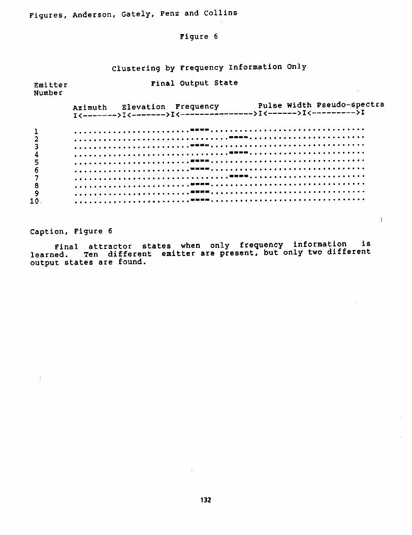
Suppose we simply learn frequent 7 iinformation. Figure 6 shows the total numberof attractors formed when ten new_ examples of each of ten emitters were passed

through the BSB dynamics, using the matrix formed from learning the pulses in thepulse buffer. In a system that clustered perfectly, exactly 10 final states wouldexist, one different final state for each of the ten emitters. However, with onlyfrequency information learned, all the 100 different inputs mapped into only two

attractors.

Figure 6 about here

Figure 6 and others like it below are graphical indications of the similaritybetween recalled clusters or states vlth computational energy minima. The states

shown in the figures are ordered via a priori knowledge of the emitters, althoughthis information was obviously not given to the network. One can visually interpret

the outputs for equality of two emitters (lumping of different emitters) or

separation of outputs for a single emitter (_ of the same emitter) in theoutputs. This display method is for the reader's benefit. _he ANSP systemdetermines the number and state vector of separate minima by a dot product search of

the entire output list, as discussed above. Position of the bar of 'ffi'scodes thefrequency in the frequency field which is the only field learned in this example.

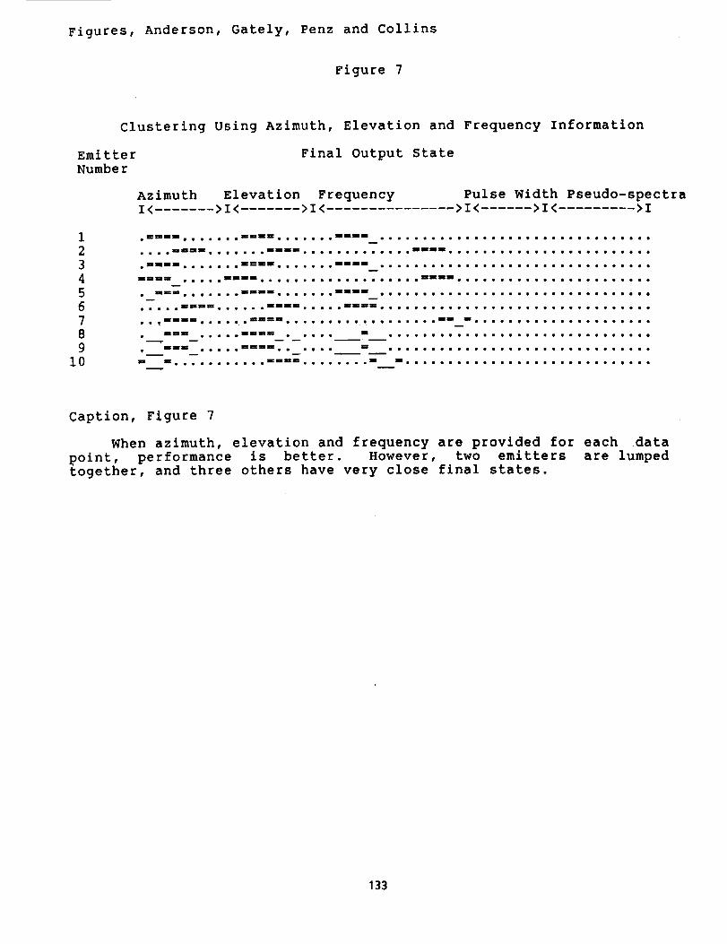
Let us now give the system additional information about pulse azimuth andelevation. Clustering performance improves markedly, as shown in Figure 7. Ne getnine different attractors. There is _till uncertainty in the system, however, since

few corners are fully saturated, as indicated by the underline symbols on the cornersof some bar's. States 1 and 3 are in the same attractor, an example of incorrect

_lumplng' as a result of insufficient information. Two other final states (8 and 9)are very close to each other in Hamming distance.

Figure 7 about here

Let us assume that future advances in receivers will allow a quick estimation of

the mlcrostructure of each radar pulse. We have used, as shown in Figure 8, a coding

which is a crude graphical version of a Fourier anlysis of an individual pulse, withthe center frequency located at the middle of the field. Emitter pulse spectra were

assigned arbitrarily.

" 117

Figure 8 about here

Note that the spectral information can be included in the state vector in onlyslightly processed form: we have included almost a caricature of the actualspectrum.

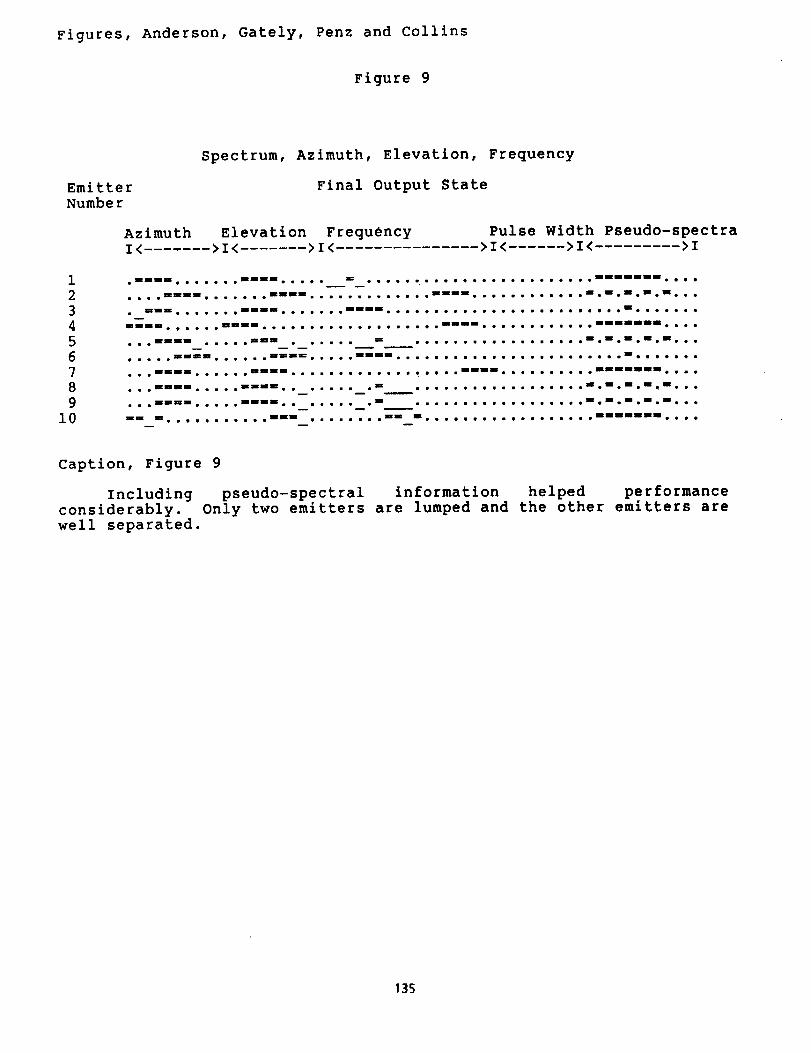
Addition of spectral information improved performance somewhat. There were ninedistinct attractors, though still many unsaturated states. Two emitters were still'lumped', 8 and 9. Figure 9 shows the results.

Figure 9 about here

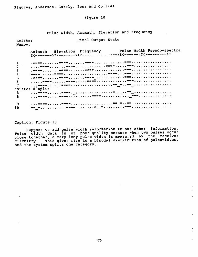
Suppose we add information about pulse width to azimuth, elevation, andfrequency. The simulated pulse width informatlon_ery poor. It actually degradesperformance, though it does allow separation of a couple of nearby emitters. Theresults are given in Figure 10.

Figure 10 about here

The reason pulse width data is of poor quality and hurts discrimination isbecause of a common artifact due to the way that pulse width is measured. When two

pulses occur close together in time a very long pulse width is measured by thereceiver circuitry. This can give rise in unfavorable cases to a spurious bimodaldistribution of pulsewidths for a single emitter. Therefore, a single emitter seemsto have some short pulse widths and some very long pulse widths and this can splitthe category. Bimodal distributions of an emitter parameter, when the peaks arewidely separated, is a hard problem for any clustering algorithm. A couple ofdifficult discriminations in this simulation, however, are aided by the additionaldata.

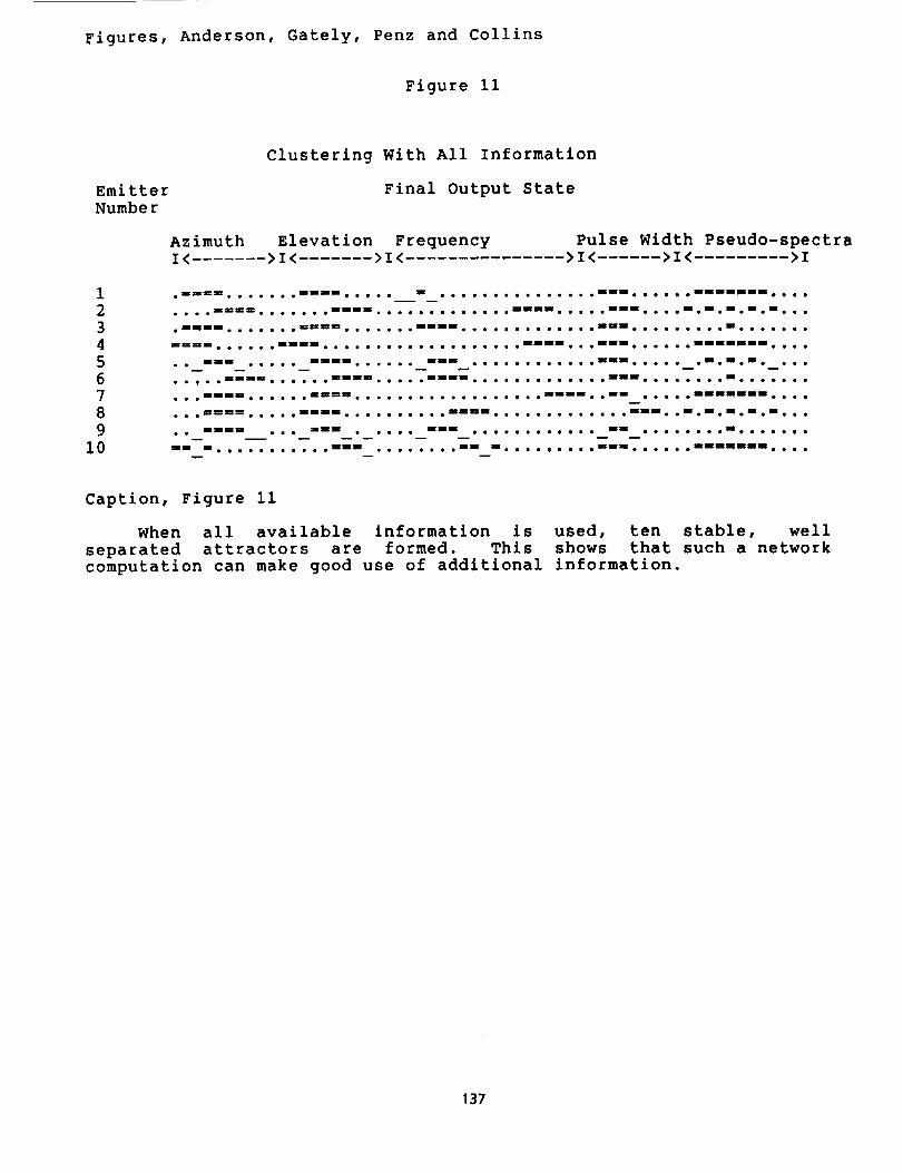
We nov combine all this information about pulse properties together. None ofthe subsets of inir6-_mation could perfectly cluster the emitters. Pulse width, inparticular, actually hurt performance. Figure 11 shows that, after learning, usingall the information, we nov get ten well separated attractors, i.e. the correctnumber of emitters relative to the data set. The conclusion is that the additionalinformation, even if it was noisy, could be used effectively. Poor information couldbe combined with other poor information to give good results.

118

Figure ii about here

Processing After Delnterleaving. Having used the ANSP system to delnterleaveand cluster da_-a[ we also have a way of producing an accurate picture of each

emitter. We now have an estimate of the frequency and pulse width and can derive

other emitter properties (Penz et._ al., 1989), for example, the emitter pulse

repetition pattern. One method to learn this pattern is to learn pulse repetitioninterval (PRI) pairs autoassociatively. Another is to autocorrelate the PRI's of a

string. This technique probably provides more information than any other forcharacterizing emitters, because the resulting correlation functions are very useful

for characterizing a particular emitter type.

Classification Problem and Neural Network Data Bases. The next task is to

classify the observed emitters ba-sed on our p-_evouT'6"d"s_xperiencewith emitters of

various types. We continue with the neural network approach because of the ability

of networks to incorporate a great deal of information from different sensors, their

ability to generalize (i.e. _guess') based on noisy or incomplete information, andtheir ability to handle ambiguity. Known disadvantages of neural networks used asdata bases are their slow computation using traditional computer architectures,

erroneous generalizations (i.e. _bad guesses'), their unpredictability, and thedifficulty of adding new information to them, which may require time consuming

relearning.

Information, in traditional expert systems, is often represented as collectionsof atomic facts, relating pairs or small sets of items together. Expert systems

often assume 'IF (x) THEN (y)' kinds of information representation. For example,

such a rule in radar might look like:

IF (Frequency is 10 gHz)AND (Pulse Width is 1 microsecond)

AND (PRI is constant at 1 kHz)

THEN (Emitter is a Klingon air traffic control radar).

Problems with this approach are that rules usually have many exceptions, data

may be erroneous or noisy, and emitter parameters may be changed because of localconditions. Expert systems may be exceptionally prone to confusion when emitter

properties change because of the rigidity of their data representation. Neuralnetworks allow a different strategy: Always try to use as much information as you

have, because, in most cases, the more information you have, the better performancewill be.

As William James commented in the nineteenth century,

... the more other facts a fact is associated with in the mind,

the 5"6_te_poses----_io--n---6f-1"_-'-ou'-'r_r-6taln---6. -Ea--_ olr-i'_a--_oc_becomes a hoo_--to"whic-_--it_, a m_ to fish it

up by when sunk beneath the surface. Together, they form a

network of attachments by which it is woven into the entire

119

tissue of our thought.William James (1890). p. 301

Perhaps, as William James suggests, information is best represented as largesets of correlated information. We could represent this in a neural network by a

large, multimodal state vector. Each state vector contains a large number of _atomlc

facts' together with their cross correlations. Our clustering demonstration showedthat more information could be added and used efficiently and that identification

depends on a cluster of information co-occurlng. (See Anderson, 1986 for further

discussion of neural network data bases of this type.)

Ultimately, we would llke a system that would tentatively

based on measured properties and previously known information.

operation, that parameters can and often do change, we can never

answers.

identify emitters

Since we know, in

be sure of the

As a specific important example, radar systems can shift parameters in ways

consistent with their physical design, that is, wavegulde sizes, power supply size,

and so on, for a number of reasons, for example, weather conditions. If an emitter

is characterized by only one parameter, and that parameter is changed, then

identification becomes very unlikely. Therefore, accuracy of measurement of a

partlcular parameter may not be as useful for classification as one might expect.

However, using a whole set of co-occurlng properties, each at low precision, may

prove a much more efficient strategy for identification. For further discussion of

how humans often seem to use such a strategy in perception, consult George Miller's

classic 1956 paper, "The magic number seven, plus or minus two."

Classification Problem for Shifted Emitters. Our first neural net

ciasslflcation simulation is s'_clflcally designed to study sensitivity to shifts in

parameters. Two data sets were generated. One set has _normal' emitter properties

and the other set had all the emitter properties changed about I0 percent. The two

sets each contained about 500 data points. The names used are totally arbitrary.

The state vector was constructed of a name string (the first I0 characters) and bar

codes for frequency, pulse width, and pulse repetition interval. For the

classification function, the position of "+" symbols indicates the feature magnitude

while the blank symbol fills the rest of the feature field. Again the "_" symbol

indicates an undecided node.

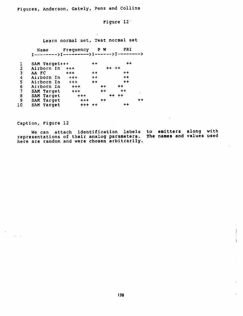
Figures 12 and 13 show the resulting attractor interpretations. Figure 12 showsthe vectors to be learned autoassociatively by the BSB model. The first field is theemitter name. The last three fields represent the numerical information produced by

the deinterleaver and pulse repetition interval modules. An input consists of

leaving the identification blank and filling in the analog information for theemitter which one wafits an identification. The autoassocative connections fill in

the missing identification information.

Figure 12 shows the identifications produced when the normal set is provided tothe matrix: all the names are produced correctly and in a small number of iterations

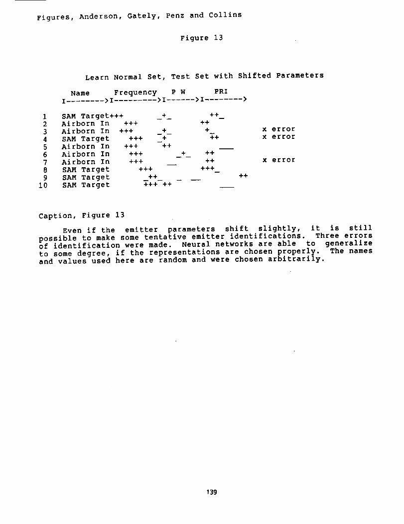
through the BSB algorithm. Figure 13 uses the same matrix, but the input data is nowderived from sources whose mean values are shifted about 10 percent, to emulate this

parameter shift.

120



There were three errors of classification. Emitter 3 was classified as 'Airborn In'

instead of 'AA FC'. Emittter 4 was classified as 'SAM target' instead of _Airborn

In'. Emitter 7 was classified as 'Airborn In' rather than the correct 'SAM Target'name. Note that the recalled analog information is also not exactly the correctanalog information even for the correctly identified emitters. At a finer scale, the

number of iterations required to reach an attractor state was very long. This is adirect measure of the uncertainty of the neural network about the shifted data. Some

of the final states were not fully limited, another indication of uncertainty.

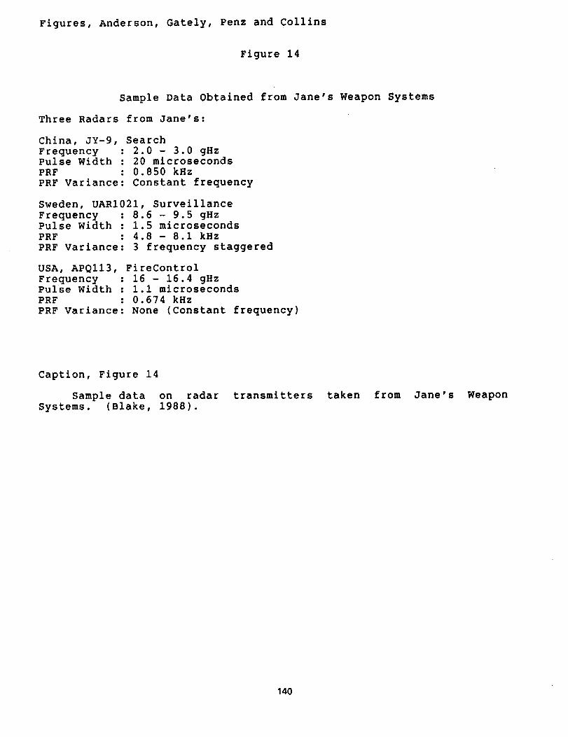
Large Classification Data Bases. it would be of interest to see how the systemworked with a larger data b---_. Some information about radar systems is published in

Jane's Weapon Systems !Blake, 1988). We can use this data as a starting point to seea neur--u-{a_networkmlght scale to larger systems. Figure 14 shows the kind of data

available from Jane's. Some radars have constant pulse repetition frequency (PRF)and others have highly variable PRF's. (Jane's lists Pulse Repetition Frequency(PRF) in its tables instead of Pulse Repetition interval (PRI). We have used their

term for their data in this simulation.) We represented PRF variability in the state

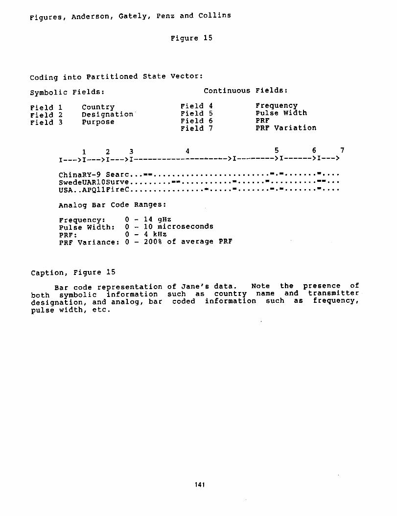
vector coding by increasing the last bar width (Field 7, Figure 15) for highlyvariable PRF's (see the Swedish radar, for an example.) Also, when a parameter is outof range (the average PRF of the Swedish radar) it is not represented.



We perform the usual partitioning of the state vector into fields, as shown inFigure 15. For this simulation, the frequency scale is so coarse that even enormouschanges in frequency would not change the bar coding significantly. We are more

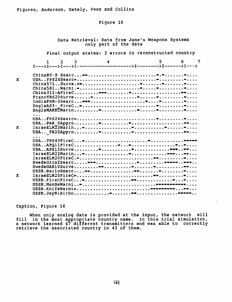
interested here in whether the system can handle large amounts of Jane's data. Wetaught the network 47 different kinds of radar transmitters. Some transmitter names

were represented by more than one state vector because they can have several, quitedifferent modes of operation, that is, the parameter part of the code can differ

significantly from mode to mode. (The clustering algorithms would almost surely pick

121

up different modes as different clusters.) After learning, we provided the measuredproperties to the the transmitter to see if it could regenerate the name of the

country that the radar belonged to. There were only three errors of retrieval from47 sets of input data, corresponding to 94 percent accurate country identification.

This experiment was basically coding a lookup table, using low precisionrepresentations of the parameters. Figure 16 shows a sample of the output, with

reconstructions of the country, designations, and functions.


Conclusions. We have presented a system using neural networks which is capable

of clustering and identifying radar emitters, given as input data large numbers ofreceived radar pulses and with some knowledge of previously characterized emitter

types.

Good features of this system are its robustness, its ability to integrateinformation from co-occurance of many features, and its ability to integrateinformation from individual data samples.

We might point out that the radar problem is similar to data analysis problemsin other areas. For example, it is very similar to a problem in experimentalneurophyslology, where action potentials from multiple neurons are recorded with a

single electrode. Applications of the neural network techniques described here maynot be limited to radar signal processing.

References

Anderson, J.A. (1972), A simple neural network generating an interactive

memory, Mathematical Biosciences, 14, 197-220.

Anderson, J.A. (1983), Neural models for cognitive computation. IEEE

Transactions: Systems r Man, and Cybernetics, SMC-13, 799-815.

Anderson, J.A. (1986), Cognitive Capabilities of a Parallel System. In E.Bienenstock, F. Foglemann, and G. Weisbuch. (Eds.) Disordered Systems and

Bio!9/_ical Organization, Berlin: Springer.

Anderson, J.A. (1987), Concept formation in neural networks: Implications for

evolution of cognitive functions. Human Eyolut{o n, 2, i987.

Anderson, J.A. and Hozer, M.C. (1989), Categorization and selective neurons,

In: G.E. Hinton and J.A. Anderson (Editors), Parallel Models of Associative Memor[_Rev. Ed.), Hillsdale, NJ: Erlbaum.

Anderson, J.A. and Murphy, G.L. (1986), Psychological Concepts in a ParallelSystem. In J.D. Farmer, A. Lapedes, N. Packard, and B. Wendroff. (Eds.)

Evolution_ Games L and Learning.. New York: North Holland.

122

Anderson, J.A. and Rosenfeld, E., Eds.

Research, Cambridge, MA: MIT Press.(1988) Neurocomputing: Foundations of

Anderson, J.A., Silverstein, J.W, Ritz, S.A., and Jones, R.S., Distinctive

features, categorical perception, and probability learning: Some applications of a

neural model, Psychological Review, 84, 413-451.

Baldi, P. and Hornik, K. (1989), Neural networks and principal component

analysis: Learning from examples without local minima. Neural Networks, 2, 53.

Blake, B. (Editor), (1988), Jane's Weapon Systems, (19th Edition), Surrey,U.K,: Jane's Information Group.

Carpenter, G. and Grossberg, S. (1987), ART 2: self organization of stable

category recognition codes for analog input patterns, Applied Optics, 26, 4919-4942.

Cottrell, G.W., Munro, P.W. and Zipser, D. (1988). Image compression by back

propagation: A demonstration of extensional programming. In N.E. Sharkey (Ed.),

Advances in Cognitive Science_ Vol. 3. Norwood, NJ: Ablex.

Golden, R.M. (1986), The "Brain state in a box" neural model is a gradient

descent algorithm, Journal of Mathematical Psychology, 30, 73-80.

Hinton, G.E. and Anderson, J.A. (Eds., 1989), Parallel Models

Memor__(Rev. Ed_._/,Hillsdale, NJ: Erlbaum.

James, g. (1961/1894), Briefer Psycholo$7, New York: Collier.

of Associative

Knapp A. and Anderson, J.A. (1984), A theory of categorization based on

distributed memory storage. Journal of Experimental Psychology: Learning, Memoryand Cognition. 2, 610-622.

Kohonen, T. (1972). Correlation matrix memories, IEEE

Computers , C-21, 353-359.

Kohonen, T. (1977). Associative Memory, Berlin: Springer.

Kohonen, T. (1984). Self Organization and AssociativeSpringer.

Transactions on

Memory. Berlin:

McClelland, J.L. and Rumelhart, D.E., Eds.

Processing, Volume 2, Cambridge, MA: MIT Press.(1986), Parallel r Distributed

Miller, G.A. (1956), The magic number seven, plus or minus two: Some limits on

our capacity for processing information, Psychological Review,63, 81-97.

Penz, P.A. (1987), The closeness code, Proceedings of IEEE InternationalConference on Neural Networks, III-515, IEEE Catalog 87th0191--7.

Penz, P.A., Katz, A.J., Gately, M.T., Collins, D.R. and Anderson, J.A. (1989),Analog capabilities of the BSB model as applied to the antl-radlatlon homing missile

problem, Proceedings of the International Joint Conference on Neural Net.___ss,II-7.

Rossen, M.L. (1989). Speech Syllable Recognition with a Neural Network, Ph.D.Thesis, Department of Psychology, Brown University, Providence, RI 02912, May, 1989.

123

Rumelhart, D.E. and McClelland, J.L., Eds.

Processing, Volume I, Cambridge, MA: MIT Press.

(1986), Parallel r Distributed

Rumelhart, D.E. and Zipser, D. (1986), Feature discovery by competitivelearning, In D.E. Rumelhart, and J.L. McClelland, Eds., Parallel_ DistributedProcessing,. Volume i, Cambridge, MA: MIT Press.

Sereno, M.E. (1989)A Neural Network Model of Visual Motion Processing, Ph.D.Thesis, Department of Psychology, Brown University, Providence, RI, May, 1989.

Viscuso, S.R., Anderson, J.A. and Spoehr, K.T., (1989) Representing simplearithmetic in neural networks, In G. Tiberghien, Ed., Advanced Cognitive Science:

Theory and Applications , London: Horwoods.

124

Figures for

Radar Signal Categorization using a Neural Network

James A. Anderson

Department of Cognitive and Linguistic Sciences

Box 1978

Brown University, Providence, RI 02912

and

Michael T. Gately, P. Andrew Penz, and Dean R. Collins

Central Research Laboratories, Texas Instruments

Dallas, Texas 75265

125

Figures, Anderson, Gately, Penz and Collins

Caption, Figure 1

Block diagram of the radar clustering and categorizing system.

Caption, Figure 2

Landscape surface of system energy. Several learned examples maycontribute to the formation of a single energy minimum which will

correspond to a single emitter. This drawing is only for illustrative

purposes and is not meant to represent the very high dimensionalsimulations actually used.

!

Caption, Figure 3

The Widrow-Hoff procedure learns the error vector. The error

vectors early in learning with a small learning constant point toward

examples, and the average of the error vectors will point toward the

category mean, i.e. all the examples of a single emitter.

Caption, Figure 4

Assume an eigenvector is close to a category mean, as will be theresult after extensive error correcting, autoassociative learning.

The error terms from many learned examples, with a small learningconstant, will average to zero and the system attractor structure will

not change markedly. (There are very long term 'senility' mechanismswith continued learning, but they are not of practical importance for

this application.)

126

©

Z©

Z

<

Q

_0

v

"'- Ur

<

1,1111

c_

rj

F.,

0 <

0

127

0

o

.,-, _0

_uao,-q

_o

•_ _0 o o_:_, ._ _I o

• _-,,a

M _ua

0o_,,_

c_o0

r_

128

0

o _

10

o

o0

,-1

129

0

r

130


Figure 5

Radar Pulse Fields: Coding of Input Information

Position of the bar of '-' codes an analog quanitity

Azimuth Elevation Frequency Pulse Width Pseudo-spectra

I< ....... >I< ....... >I< ........... >I< .......... >I< ......... >I

..oNJ|noopoo|mnnooeoooooo_s|i|oeeeoooeooeoo|||oJ|Ono|.|.|-oo

In any field: A move to the left decreases the quantity

A move to the right increases the quantity

Caption, Figure 5

Input representation of analog input data uses bar codes. The

state vector is partitioned into fields, corresponding to azimuth,

elevation, frequency, pulse width, and a field corresponding toadditional information that might become available with advances in

receiver technology.

131


Figure 6

Emitter

Number

123

45

67

89

i0,

Clustering by Frequency Information Only

Final Output State

Azimuth Elevation Frequency Pulse Width Pseudo-spectrai< ....... >I< ........ >I< ............... >I< ...... >I<--- ...... >I

Caption, Figure 6

Final attractor states when only frequency information is

learned. Ten different emitter are present, but only two differentoutput states are found.

132


Figure 7

Clustering Using Azimuth, Elevation and Frequency Information

EmitterNumber

Final Output State

Azimuth Elevation Frequency Pulse Width Pseudo-spectraI< ....... >I< ....... >I< ............... >I<- >I< --->I

67

89

i0

Caption, Figure 7

When azimuth, elevation and frequency are provided for each data

point, performance is better• However, two emitters are lumpedtogether, and three others have very close final states•

133


Figure 8

a)

b)

c)

Q.oeeom.oeeBO

e.memt_om.moe

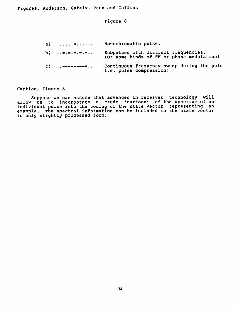
Monochromatic pulse.

Subpulses with distinct frequencies.(Or some kinds of FM or phase modulation)

Continuous frequency sweep during the puls

i.e. pulse compression)

Caption, Figure 8

Suppose we can assume that advances in receiver technology willallow us to incorporate a crude 'cartoon' of the spectrum of an

individual pulse into the coding of the state vector representing anexample. The spectral information can be included in the state vector

in only slightly processed form.

134


Figure 9

Spectrum, Azimuth, Elevation, Frequency

Emitter Final Output State

Number

Azimuth Elevation Frequency Pulse Width Pseudo-spectraI< ....... >I< ....... >I< .......... >I<- >I< ......... >I

1

234

5

67

8

9i0

Caption, Figure 9

Including pseudo-spectral

considerably• Only two emitters

well separated•

information helped

are lumped and the other

performanceemitters are

135


Figure i0

Pulse Width, Azimuth, Elevation and Frequency

Emitter Final Output StateNumber

Azimuth Elevation FrequencyI< ....... >I< ....... >I< ........

Pulse Width Pseudo-spectra>I< ...... >I< ......... >I

123

45

67

Emitter

8

8

9

i0

Caption, Figure 10

Suppose we add pulse width information to our other information.Pulse width data is of poor quality because when two pulses occur

close together, a very long pulse width is measured by the receivercircuitry. This gives rise to a bimodal distribution of pulsewidths,

and the system splits one category.

136


Figure ii

Clustering With All Information

Emitter Final Output StateNumber

Azimuth Elevation Frequency Pulse Width Pseudo-spectraI< ....... >I< >I< ...... >I< >I< >I

6

789

i0

I|B||•o•••I•BBBBI•II• B •••lllllllllllli|i•lllllBBBBJJU(lll

•.e•Bmim•o•••oolUmB•ooo_•••O,•l.emnJowwoomBmooe_menoloBomo••

•I_BB••O••••BBNNww•.•ooNBBBg•OBOU.IWWW.wBNB•_e_O•OBOU_OQOO

lmBmo_••••BBn_,ooili•••••••igggoimmmeeunBmi0_0o0mIllIiUo_•_

W n._ Big •••I, _lmm....•• SIS oww.ll..leolnmBo•••• • • •m o ••_

.oQoeBBBBmIOlUOBBB|.OIOoBB|NoooewvvIoooooBBBooulooooNoooolOO

..wi. .. ...oo • BBu BBee. o• o! o.e

,•.BBB_,..,,B ,,.,. .S KS .. .. B B• So.

o. BnBB ,,, gum , ,,,, Bnu o,,,,,,oooo, Is ,,,,eeooUoo.,o,o

Bm BO•OBIIgeee,BBB .,.•.!BOMB laoooee0o.BmB••••eoNBB_lJmoo,e

Caption, Figure 11

When all available information is used, ten stable, well

separated attractors are formed. This shows that such a networkcomputation can make good use of additional information•

137


Figure 12

Learn normal set, Test normal set

Name Frequency P W PRII ........ >I ......... >I ...... >I ........ >

1 SAM Target+++ ++2 Airborn In +++

3 AA FC +++ ++

4 Airborn In +++ ++

5 Airborn In +++ ++

6 Airborn In +++

7 SAM Target +++

8 SAM Target +++

9 SAM Target +++

10 SAM Target +++ ++

++

++ ++

++

++

++

++ ++

++ ++

++ ++

++

++

++

Caption, Figure 12

We can attach identification labels

representations of their analog parameters.here are random and were chosen arbitrarily.

to emitters along withThe names and values used

138


Figure 13

Learn Normal Set, Test Set with Shifted Parameters

Name Frequency P W PRII........ >I >I ...... >I- >

1 SAM Target+++ _+_ ++_2 Airborn In +++ ++3 Airborn In +++ + + x error

4 SAM Target +++ + ++ x error5 Airborn In +++ ++

6 Airborn In +++ + ++7 Airborn In +++ ++ x error

8 SAM Target +++ +++

9 SAM Target ++ ++i0 SAM Target _++--++

Caption, Figure 13

Even if the emitter parameters shift slightly, it is still

possible to make some tentative emitter identifications. Three errorsof identification were made. Neural networks are able to generalize

to some degree, if the representations are chosen properly. The namesand values used here are random and were chosen arbitrarily.

139


Figure 14

Sample Data Obtained from Jane's Weapon Systems

Three Radars from Jane's:

China, JY-9, Search

Frequency : 2.0 - 3.0 gHzPulse Width : 20 microseconds

PRF : 0.850 kHz

PRF Variance: Constant frequency

Sweden, UARI021, Surveillance

Frequency : 8.6 - 9.5 gHzPulse Width : 1.5 microseconds

PRF : 4.8 - 8.1 kHz

PRF Variance: 3 frequency staggered

USA, APQII3, FireControl

Frequency : 16 - 16.4 gHzPulse Width : I.i microseconds

PRF : 0.674 kHz

PRF Variance: None (Constant frequency)

Caption, Figure 14

Sample data on radar

Systems. (Blake, 1988).

transmitters taken from Jane's Weapon


Figure 15

Coding into Partitioned State Vector:

Symbolic Fields: Continuous Fields:

Field 4 FrequencyField 5 Pulse Width

Field 6 PRF

Field 7 PRF Variation

Field 1

Field 2

Field 3

Country

Designation

Purpose

1 2 3 4

I---> I---> I---> I--

5 6 7

.... >I ........ >I ...... >I--->

ChinaRY-9 Searc...--. ........................ "-" ....... ",...

SwedeUARl0Surve ......... -- ........... " ...... " .......... "''''

USA..APQIIFireC ................ - ..... " ....... -." ....... " ....

Analog Bar Code Ranges:

Frequency: 0 -Pulse Width: 0 -

PRF: 0 -

PRF Variance: 0 -

14 gHzi0 microseconds

4 kHz

200% of average PRF

Caption, Figure 15

Bar code representation

both symbolic information

designation, and analog, bar

pulse width, etc.

of Jane's data. Note the presence of

such as country name and transmitter

coded information such as frequency,

141


Figure 16

X

X

X

Data Retrieval: Data from Jane's Weapons Systems

only part of the data

Final output states: 3 errors in reconstructed country

1 2 3 4 5 6 7

I---> I---> I---> I--" ................. >I ........ >I ...... >I--->

ChinaRY-9 Searc.. -- ......................... -.- ....... - ....

USA..FPS24Searc-. ............................ - ......... - ....

China571..Surve.-- ..................... - ....... - ....... - ....

China581..Warni.- ...................... - ..... - ......... - ....

China311-AFireC ......... --- ........ - .................. --....

FrancTRS20Surve ...... - ................ - ...... - ......... - ....

IndiaPSM-3Searc...--- .................... - .... - ........ - ....

EnglaAS3- FireC..- ........................... - ......... - ....

EnglaMARECMarin ......... - ............. - ...... - ......... - ....

USA..FPS24Searc- ............................. - ......... - ....

USA..PAR 0Appro ......... - .......... - ................... --...IsraeELM_2Marin...- ................. - ........... - ...... - ....

USA.. PR20Appro ......... - ........... - .................. --...

ggQ

USA..TPS43FireC...- ....................... - ............ - ....

USA..APQIIFireC ................ -...- ................ -..- ....USA..APSI2Surve ......... t ........... . ............. ---..--...

IsraeELM22Marin...- ................ - ............. ---...--...

IsraeELM20FireC.- ........................... -- ......... - ....

SwedeGirafSearc ..... ---. .............. - ......... -----..---..

SwedeUARl0Surve ......... -- .......... - ....... - .......... --...

USSR.BarloSearc .... -- ................ -- ....... - ........ - ....

IsraeELM20FireC- ............................ -- ......... - ....

USSR.FireCFireC...- ................. -- ............. -...- ....

USSR.HenSeWarni..- ........................... ------- .... ....

USSR.KnifeWarni-. .......................... ---------...--...

USSR.JayBiAirbo ............. - ....... -- ............... -----..

Caption, Figure 16

When only analog data is provided at the input, the network will

fill in the most appropriate country name. In this trial simulation,

a network learned 47 different transmitters and was able to correctly

retrieve the associated country in 43 of them.

142

N91- lTS - NASA

Documents