,N81 -14696 ':V~ - NASA to jet deflector nozzle flow in VTOL aircraft. The portion of a grid shown in the adjacent figure was used for this calculation. The 90 deg elbow demonstrates

,N81 -14696 ':V~ - -

fINITE DIFFERENCE GRID GENERATION BY MULTIVARIATE BLENDING FUNCTIO~ INTERPOLATION*

Peter G. Anderson and Lawrence W. Spradley Lockheed-Huntsville Research & Engineering Center

Huntsville, Alahama

ABSTRACT

.., ..... " "

The General Interpolants Method (GIM) code solves the multi­

dimensional Navier-Stokes equations for arbitrary geometric domains.

The geometry module in the GIM code generates two- and three­

dimensional grids over specified flow regimes, establishes boundary

condition information and computes finite difference analogs for use in

the GIM code numerical solution module. The technique can be classified

as an algebraic equation approach.

The geometry package uses multivariate blending function interpola­

tion of vector-values functions which define the shapes of the edges and

surfaces bounding the flow domain. By employing blending functions

which conform to the cardinality conditions the flow domain may be mapped

onto a unit square (2-D) or unit cube (3 -D), thus producing an intrinsic

_- coordinate system for the region of interest. The intrinsic coordinate

system facilitates grid spacing control to allow for optimum distribution

of nodes in the flow domain.

The GIM formulation is not a finite element method in the classical

sense. Rather, finite difference methods are used exclusively but with the

difference equations written in general curvilinear coordinates. Trans­

formations are used to locally transform the physical planes into regions

of unit cubes. The mesh is generated on this unit cube and local metric-

like coefficients generated. Each region of the flow domain is likewise

transformed and then blended via the finite element formulation to form

the full flow domain. In order to treat "completely-arbitrary" geometric

domains, different transformation functions can be employed in different

regions. We then transform the blended domain to physical space and solve

the Cartesian set of equations for the full region. The geometry part of the

problem is thus treated much like a finite element technique while integration

of the equations is done with finite difference analogs.

*This work was supported, in payt, by NASA Langley Contracts NAS1-15341, 15783, and 15795.

143

https://ntrs.nasa.gov/search.jsp?R=19810006182 2018-06-20T21:20:37+00:00Z

144

BU I LD I NG BLOCK CONCEPT

The development is done in local curvilinear intrinsic coordinates based

on the following concepts:

• Analytical regions such as rectangles, spheres, cylinders, hexahedrals, etc., have intrinsic or natural coordinates.

• Complex regions can be subdivided into a number of smaller regions which can be described by analytic functions. The degenerate caSe is to subdivide small enough to use very small straight-line segments.

• Intrinsic curvilinear coordinate systems result in constant coordinate lines throughout a simply connected, bounded domain in Euclidean space.

• The inter section of the lines of constant coordinates produce nodal points evenly spaced in the domain.

• Intrinsic curvilinear coordinate systems can be pro­duced by a univalent mapping of a unit cube onto the simply connected bounded domain.

Thus, if a transformation can be found which will map a unit cube uni­

valently onto a general analytical domain, then any complex region can be

piecewise transformed and blended using general interpolants.

Consider the general hexahedral configuration shown. The local intrinsic

coordinates are 111,112,113 with origin at point PI' The shape of the geometry

is defined by

• Eight corner points, P. 1

• Twelve edge functions, E. 1

• Six surface functions, S. 1

This shape is then fully described if the edges and surfaces can be specified

as continuous analytic vector functions S. (x, y, z), E. (x, y, z), 1 1

BUILDING BLOCK CONCEPT

P.4..--____ -. P 3

a. Point Designations

E 3

b. Edgl! Designations

c. Surface Designations

145

146

GENERAL INTERPOLANT FUNCTION

Based on the work of Gordon and Hall we have developed a general

relationship between physical Cartesian space and local curvilinear intrinsic

coordinates. This relation is given by the general trilinear interpolant shown

on the adjac ent figure.

In this equation, ~ vector is the Cartesian coordinates

and Si' Ei are the vector functions defining the surfaces and edges, respectively,

and Pi are the (x,y, z) coordinates of the corner points. Edge and surface func­

tions that are currently included in the GIM code are the following:

• EDGES (Combinations of up to Five Types)

Linear Segment Circular Arc Conic (Elliptical, Parabolic, Hyperbolic) Helical Arc Sinu soldal Segment

• SURF ACES (Bounded by Above Edges)

Flat Plate Cylindrical Surface Edge of Revolution

This library of available functions is simply called upon piecewise via input

to the computer code.

With this transformation, any point in local coordinates 1']1' 1']2' 1']3 can

be related to global Cartesian coordinates x, y, z. Likewise any derivatives

of functions in local coordinates can be related to that derivative in physical

space.

GENERAL INTERPOLANT FUNCT ION

-' -l -"

- (1 -7) 2.) 11 3 E 9 - , I 2. (1 - Ii 3) E 3 - 11 Z I') 3 E 1 }

"-.-.,----

--' -"

+ (1-1/1) III (1-1/3) P4 + (1-1/\) I)l 1/ 3 P s

-" -" + IiI (I-Ill) (1-1J 3) P z + IiI (I-liZ) 1')3 P 6

...... + II} I1 Z (1-1/3) P 3 + III liZ 1)3 P7

----,,'

147

148

INTERNAL FLOW GRID (Axisymmetric Rocket Nozzle)

The grid shown was used to compute the flow in a model of the Space

Shuttle engine us ing the GIM code. The mesh is stretched in the radial direc­

tion to cluster points near the wall and stretched axially to place points near

the throat of the nozzle. Only a portion of the complete grid is shown for

clarity and illustration. The grid shows the general format used by the GIM

code for internal, two-dimensional flows in non-rectangular shapes.

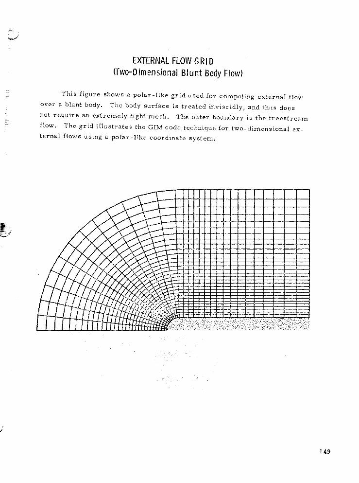
EXTERNAL FLOW G RID (Two-Dimensional BI unt Body Flow)

This figure shows a polar-like grid used for computing external flow

over a blunt body. The body surface is treated invlscidly, and thus does

nOt require an extremely tight mesh. The outer boundary is the freestream

flow. The grid illustrates the GIM code technique for two-dimensional ex­

ternal flows using a polar-like coordinate system.

149

150

EXTERNAL FLOW G RID (Non-Orthogonal Cu rvilinear Coordinates)

The nodal network for the external flow over an ogive cylinder illustrates

the capability of the GIM code geometry package to stretch the nodal distribu­

tion. The grid is very compact in the leading edge region and greatly expanded

in the far field areas, The axial points follow the body surface and could gen­

erally be called ., body-oriented coordinates" in the nomenclature of the litera­

ture. The radial grid lines are not necessarily normal to the lateral lines or

to the body surface. The GIM code, through its tlnodal-analog" concept can

operate on this general non-orthogonal curvilinear grid.

OIUGF:.:\L r / .~~ IS .O~ r'\=<)l'( (:';_':k\·~.:":"'··-[

1/ """-"

THREE-DIMENSIONAL GRID (Simple Rectilinear Coordinates)

Supersonic flow in expanding ducts of arbitrary crOss section is a common

occurrence in computational fluid dynamics. This figure illustrates a simple

grid for a three-dimensional duct whose cross section varies sinusoidally with

the axial coordinate. The 11 top" wall and the "front" wall have this sinusoidal

variation while the "bottom" and "back" walls are flat plates. The grid shown

was used to resolve the expanding-recompressing supersonic flow including the

intersection of the two shock sheets.

151

152

THREE-D IMENSIONAL GRID (Pipe Flow in a 90 deg ElbowTurn)

There are numerous flow fields of interest which contain a sharp turn

inside a smooth pipe. The GIM code has treated certain of these for applica­

tion to jet deflector nozzle flow in VTOL aircraft. The portion of a grid shown

in the adjacent figure was used for this calculation.

The 90 deg elbow demonstrates the capability to model three-dimensional

non-Cartesian geometries. The internal nodes were emitted for clarity. The

elbow grid was generated by employing edge-oI-revolution surfaces with circular

arc segments as the edges being revolved.

GRID FOR SPACE SHUTILE MAIN ENGINE (Hot Gas Manifold Geometry Model)

The recent problems encountered with the Space Shuttle main engine

tests have resulted in a GIM code analysis of the system. The I'hot gas mani­

fold" is a portion of this analysis for the high pressure turbopump system.

The grid shown in the adjacent figure was used for this calculation. Only a

small number of nodes are shown for clarity; the full model consists of approx­

imately 14,000 nodes. The extreme complexity of this geometry illustrates

the necessity of using a GIM-like technique. Transforming this case to a

square box computational domain is, of course, impossible. The results of

the GIM code analysis agree qualitatively with flow tests that have been run

on the hot gas manifold.

Hot Gas Manifold Configuration

153

154

Inner Wall Omitted

GRID FOR SPACE SHUTTLE MAIN ENGINE (Hot Gas Manifold Geometry Model)

Outer Wall

Inner Duct

SUMMARY

• Finite difference grids can be generated for very general con­

figurations by using multivariate blending function interpolation.

• The GIM code difference scheme operates on general non­

orthogonal curvilinear coordinate grids.

• This scheme does not require a single transformation of the

flow do~nain onto a square box. Thus, GlM routines can indeed

treat arbitrary three-dimensional shapes.

• Grids generated for both internal and external flows in two and

three dimensions have shown the ver satility of the algebraic

approach.

• The GIM code integration module has successfully computed

flows on these complex grids, including the Sp:ice Shuttle

main engine turbopump system.

• Plans for future application of the code include supersonic flow

over missiles at angle of attack and three-dimensional, viscous,

reacting flows in advanced aircraft engines. Plans for future

grid generation work include schemes for time-varying networks

which adapt themselves to the dynamics of the flow.

. 155

156

BIBLIOGRAPHY

Spradley, L. W., J.F. Stalnaker and A. W. Ratliff, IIComputation of Three­Dimensional Viscous Flows with the Navier -Stokes Equations,1I AIAA Paper 80-1348, July 1980.

Spradley, L. W., and M. L. Pearson, "GIM Code User's Manual for the STAR-IOO Comp'.lter,f1 NASA-CR-3157, Langley Research Center, Hampton, Va., 1979.

Spradley, L. W., P. G. Anderson and M. L. Pearson, 11 Comp'.ltation of Three­Dimensional Nozzle-Exhaust Flows with the GIM Code,f1 NASA CR-3042, Langley Research Center, Hampton, Va., August 1978.

Prozan, R.J., L.W. Spradley, P.G. Anderso:l:lnd M.L. Pearson, TIThe General Interpolants Method," AIAA Pap'2r 77-642, June 1977.

Gordon, W.J., and C.A. Hall, "Construction:):;: Curvilinear Coordinate Systems and Applications to Mesh Generation,1I J. Numer. Math., Vol. I, 1973, pp. 461-477. ---------