N=4 super KdV hierarchy in N=4 and N=2 superspaces

arX

iv:h

ep-t

h/95

1003

3v2

11

Oct

199

5

ENSLAPP-L-554JINR-E2-95-424hep-th/9510033

October 1995

N = 4 super KdV hierarchy in N = 4 and N = 2 superspaces

F. Delduc(a), E. Ivanov(b) and S. Krivonos (b)

(a) Lab. de Phys. Theor. ENSLAPP, ENS Lyon

46 Allee d’Italie, 69364 Lyon, France

(b)Bogoliubov Laboratory of Theoretical Physics, JINR,

Dubna, 141 980 Moscow region, Russia

Abstract

We present the results of further analysis of the integrability properties of theN = 4 supersymmetric KdV equation deduced earlier by two of us (F.D. & E.I.,Phys. Lett. B 309 (1993) 312) as a hamiltonian flow on N = 4 SU(2) supercon-formal algebra in the harmonic N = 4 superspace. To make this equation and therelevant hamiltonian structures more tractable, we reformulate it in the ordinaryN = 4 and further in N = 2 superspaces. In N = 2 superspace it is representedby a coupled system of evolution equations for a general N = 2 superfield and twochiral and antichiral superfields, and involves two independent real parameters, a

and b. We construct a few first bosonic conserved charges in involution, of dimen-sions from 1 to 6, and show that they exist only for the following choices of theparameters: (i) a = 4, b = 0; (ii) a = −2, b = −6; (iii) a = −2, b = 6. The samevalues are needed for the relevant evolution equations, including N = 4 KdV itself,to be bi-hamiltonian. We demonstrate that the above three options are related viaSU(2) transformations and actually amount to the SU(2) covariant integrabilitycondition found in the harmonic superspace approach. Our results provide a strongevidence that the unique N = 4 SU(2) super KdV hierarchy exists. Upon reductionto N = 2 KdV, the above three possibilities cease to be equivalent. They give riseto the a = 4 and a = −2 N = 2 KdV hierarchies, which thus prove to be differenttruncations of the single N = 4 SU(2) KdV one.

1 Introduction

The Korteweg-de Vries (KdV) hierarchy and its supersymmetric extensions were the sub-ject of many studies for the last several years. Besides supplying nice examples of inte-grable systems, they bear a deep relation to conformal field theory, 2D gravity, matrixmodels, etc. One of the remarkable properties of these systems is that they are related,via the second hamiltonian structure, to the classical (super)conformal algebras: Virasoroalgebra in the bosonic case and N ≥ 1 superconformal ones in the case of N ≥ 1 superex-tended hierarchies [1]- [14]. Generalized KdV type systems related to Wn algebras andtheir supersymmetric extensions also received a great deal of attention (see, e.g., Ref. 15and references therein).

Up to now, supersymmetric KdV hierarchies have been constructed for N = 1, 2, 3 and4, based on the above mentioned relation to superconformal algebras [3]- [14]. An inter-esting peculiarity is that, beginning with N = 2, the supersymmetric KdV equations turnout to be integrable (give rise to the whole hierarchy or, in other words, have an infinitenumber of conservation laws in involution) only for special choices of the parameters in thehamiltonian. There exist only three integrable N = 2 KdV hierarchies: the a = 4, a = −2and a = 1 ones [8–10], with a a parameter entering into the N = 2 KdV hamiltonian,despite the fact that for any value of a the related N = 2 super KdV possesses N = 2SCA as the second hamiltonian structure. The generalized N = 2 KdV system associatedwith N = 2 W3 algebra (“N = 2 super Boussinesq hierarchy”) has similar properties asestablished in Refs. 16 and 15. For the N = 3 super KdV equation associated with N = 3SCA the requirement of integrability also strictly fixes the value of a free parameter inthe hamiltonian [13], though the existence of the whole hierarchy in this case has not yetbeen proven (the Lax pair representation has not been found). Only a few higher orderconservation laws in involution have been constructed. Nevertheless the existence of suchquantities is highly non-trivial and provides strong evidence in favour of the integrabilityof the associated N = 3 super KdV.

Another higher N extension of N = 2 super KdV, the N = 4 one, has been con-structed in the article of two of us [14]. We proceeded from the N = 4 SU(2) (”small”)superconformal algebra [17] as the second hamiltonian structure. This extension is, in asense, more economic than the N = 3 one, because N = 4 SU(2) SCA by its componentcurrents content is a natural generalization of N = 2 SCA. Like N = 2 SCA, it containsonly currents with canonical dimensions: a dimension 2 conformal stress tensor, four di-mension 3/2 fermionic currents and three dimension 1 affine su(2) currents. N = 3 SCAincludes an extra current with a subcanonical dimension 1/2 [17]. Both N = 4 SU(2) andN = 2 SCAs belong to the family of u(N) Knizhnik-Bershadsky superconformal algebras(which are nonlinear in general, starting with N = 3).

In our construction [14] we used the formalism of N = 4, 1D harmonic superspace(HSS) as the most natural one for representing N = 4 SU(2) SCA in a manifestly su-persymmetric form. We found that the general superfield N = 4 KdV hamiltonian, H3,consists of two pieces. One is an integral over the whole N = 4 HSS and the second is anintegral over an analytic subspace of this HSS, containing half the number of odd coordi-nates. This second piece involves a set of SU(2) breaking constants which are naturallycombined into a symmetric rank 4 SU(2) spinor cilkj (symmetric traceless rank 2 tensor).

1

We did not construct a Lax pair for the N = 4 KdV equation, but instead addressed thequestion of the existence of higher order conserved quantities, like in the N = 3 KdVcase [13]. We found that such quantities exist and, hence, that N = 4 KdV can lead toan integrable hierarchy, provided (i) the SU(2) breaking tensor is expressed as a square ofsome constant real SU(2) vector aij = aji, (i, j = 1, 2), and (ii) the norm of the latter isproportional to the reciprocal of the level of the affine su(2) subalgebra of N = 4 SU(2)SCA

cijkl =1

3

(

aijakl + aikajl + ailajk)

(1.1)

|a|2 ≡ −aijaij =20

k. (1.2)

We also showed that under these restrictions the N = 4 KdV equation is bi-hamiltonian,i.e. it possesses a first hamiltonian structure, the relevant hamiltonian being the dimension4 conserved charge H4 (next in dimension to H3). We considered a reduction to the N = 2case and found that, under a certain embedding of U(1) subalgebra in SU(2), the a = 4integrable version [8] of N = 2 KdV comes out.

In Ref. 14 we limited ourselves to the construction of the dimension 4 higher orderconserved charge. On the other hand, it is known that in the N = 2 case the evendimension bosonic conserved charges exist only for the a = 4 hierarchy [8, 9]. As pointedout in Ref. 14, to learn whether the other two N = 2 hierachies admit an extension toN = 4, perhaps under different restrictions on the parameters aij , the construction of thedimension 5 conserved charge for N = 4 KdV would be crucial. In the N = 2 case itexists for all three super KdV hierarchies and is given by different expressions in everycase [9]. It is very complicated to construct such a quantity directly in HSS. At the sametime, for N = 2 superfield computations there exist powerful computer methods basedon the package “Mathematica” [18]. Keeping this in mind, it is tempting to reformulateN = 4 super KdV in terms of N = 2 superfields.

This is one of the main purposes of the present paper. We rewrite the N = 4 superKdV in N = 2 superspace as a coupled system of equations for a general dimension 1superfield (this is just the N = 2 KdV superfield) and dimension 1 chiral and antichiralconjugated superfields. This system involves two independent parameters which are thecomponents of the SU(2) breaking tensor cijkl in a fixed SU(2) frame. We explicitlyconstruct the dimension 5 and 6 conserved charges for this system (beside reproducingin the N = 2 formalism the charges found in Ref. 14). They exist if and only if therestrictions (1.1), (1.2) hold. This is a very strong indication that N = 4 KdV, withconditions (1.1), (1.2), gives rise to an integrable hierarchy and that the latter is unique.One more argument in favour of the integrability is that under the same restrictions onthe parameters the N = 4 super KdV system is bi-hamiltonian. In this article we checkthis property also for the evolution equations associated with other conserved charges.One more new result of this article is the observation that two inequivalent reductionsof the same N = 4 KdV to the N = 2 one are possible. They depend on how the U(1)symmetry of the latter is embedded into the original SU(2) group. One of these reductionswas described in Ref. 14 and it leads to the a = 4, N = 2 KdV. The second one yields thea = −2, N = 2 KdV. Thus these two different N = 2 KdV hierarchies prove to originatefrom the single higher symmetry N = 4 KdV hierarchy.

2

The paper is organized as follows. In Sec. II we recall, with some further comments,the basic points of our construction of N = 4 super KdV in N = 4, 1D HSS. In Sec. IIIwe rewrite N = 4 KdV in ordinary N = 4, 1D superspace and then in N = 2 superspace,and show the possibility of two different reductions to N = 2 super KdV. In Sec. IV thedimension 4,5 and 6 conserved charges are constructed and shown to exist only with therestrictions (1.1), (1.2). Concluding remarks are collected in Sec. V. Two Appendicescontain some technical details.

2 N=4 KdV in 1D harmonic superspace

Here we recapitulate the salient features of N = 4 super KdV equation in the harmonicsuperspace formulation basically following Ref. 14. We use a slightly different notationand add some comments.

2.1. N=4 SU(2) SCA. We started in Ref. 14 with the N = 4 SU(2) superconformalalgebra. In ordinary N = 4, 1D superspace with coordinates

ZM ≡ (x, θi, θj) , (i, j = 1, 2) (2.1)

this SCA is represented by the dimension 1 supercurrent V ij(Z) = V ji(Z), (V ij)† =ǫikǫjlV

kl, satisfying the constraints (see, e.g., Ref. 19):

D(iV jk) = 0 , D(iV jk) = 0 . (2.2)

Here

Di =∂

∂θi− i

2θi

∂

∂x, Di = − ∂

∂θi

+i

2θi ∂

∂x, {Di, D

j} = i δij∂ , {Di, Dj} = 0 , (2.3)

the SU(2) indices i, j are raised and lowered by the antisymmetric tensors ǫij , ǫij (ǫijǫjk =δik , ǫ12 = −ǫ12 = 1) and (i1...in) means symmetrization (with the factor 1/n!). It is

straightforward to check that the constraints (2.2) leave in V ij only the following inde-pendent superfield projections

V ij , ξk = DiV ki , ξk = −DiV k

i , T = DiDkVik . (2.4)

The θ independent parts of these projections, wij(x), ξl(x), ξl(x), T (x), up to inessentialrescalings coincide with the currents of N = 4 SU(2) SCA: the SU(2) triplet of spin 1currents generating SU(2) affine Kac-Moody subalgebra, a complex doublet of spin 3/2currents and the spin 2 conformal stress-tensor, respectively. Superfield Poisson bracketsbetween the N = 4 SU(2) supercurrents leading to the classical N = 4 SU(2) SCA forthese component currents will be presented below.

The same N = 4 SU(2) supercurrent admits an elegant reformulation in the N = 4,1D harmonic superspace.

The latter is defined as an extension of {ZM} by the harmonic variables u±i describing

a 2-sphere ∼ SU(2)/U(1){ZM} ⇒ {ZM , u+i , u−j} ,

3

u+iu−i = 1 , u+

i u−j − u−

i u+j = ǫij (2.5)

(see Refs. 20 and 21 for details of the harmonic superspace approach).In what follows we will need the derivatives in harmonic variables which are given by

D++ ≡ ∂++ = u+i ∂

∂u−i, D−− ≡ ∂−− = u−i ∂

∂u+i

D0 = [D++, D−−] = u+i ∂

∂u+i− u−i ∂

∂u−i. (2.6)

The operator D0 measures the U(1) charge of functions on the harmonic superspace.This charge is defined as the difference between the numbers of the + and − indices. Thepreservation of this U(1) charge is one of the basic postulates of the harmonic superspaceapproach. It expresses the fact that the harmonic variables belong to the sphere S2 (actu-ally contain two independent parameters) and the harmonic superfields are functions onthis sphere as well. Let us notice that this U(1) charge commutes with the automorphismSU(2) group which acts on the doublet indices i, j.

Also, instead of Di , Dj we will use their projections on u±i

D± = Diu±i , D± = Diu±

i . (2.7)

Nonvanishing (anti)commutators of these projections with themselves and with the har-monic derivatives D++, D−− are

{D−, D+} = i∂ , {D+, D−} = −i∂ , (2.8)[

D++, D−]

= D+ ,[

D−−, D+]

= D− . (2.9)

We define now the N = 4, 1D harmonic superfield V ++(Z, u) subjected to the con-straints

D+V ++ = 0 , D+V ++ = 0 (2.10)

D++V ++ = 0 . (2.11)

(their consistency stems from the fact that the differential operators in (2.10), (2.11)are mutually (anti)commuting). The harmonic constraint (2.11) implies that V ++ is ahomogeneous function of degree 2 in u+i

V ++(Z, u) = V ij(Z) u+i u+

j . (2.12)

Then, in view of the arbitrariness of u+i, u+j, the constraints (2.10) imply for V ij theoriginal constraints (2.2). Thus the superfield V ++ obeying (2.10), (2.11) represents theN = 4 SU(2) conformal supercurrent in the harmonic 1D N = 4 superspace (see alsoRef. 22).

The constraints (2.10) can be viewed as Grassmann analyticity conditions covariantlyeliminating in V ++ the dependence on half of the original Grassmann coordinates, namely,on their u− projections θ− = θiu−

i , θ− = θiu−i . So V ++ is an analytic harmonic superfield

living on an analytic subspace containing only the u+ projections of θi , θj

{ζM} = {z, θ+, θ+, u+, u−} , (2.13)

4

z = x − i

2

(

θ+θ− + θ−θ+)

, θ± = θiu±i , θ± = θiu±

i .

This harmonic analytic superspace is closed under the action of N = 4, 1D supersymetry(and actually under the transformations of the whole N = 4 SU(2) SCA, see below).Thus, one may construct additional superinvariants as integrals over this superspace.This opportunity will be exploited when constructing the N = 4 super KdV hamiltonianand higher order conserved quantities.

In the analytic basis {z, θ±, θ±, u±i } the covariant spinor derivatives D+, D+ are re-

duced to the partial derivatives

D+ = − ∂

∂θ−, D+ = − ∂

∂θ−,

and the conditions (2.10) indeed become Grassmann Causchy - Riemann conditions stat-ing the independence of V ++ on θ−, θ− in this basis

V ++ = V ++(ζ) .

Now the irreducible components wij(x), ξl(x), ξl(x), T (x) naturally appear in the θ+, θ+

expansion of V ++ as the result of solving the harmonic constraint (2.11). The analyticity-preserving harmonic derivative D++ in the analytic basis, when acting on analytic super-fields, is given by the expression

D++ = ∂++ − iθ+θ+∂z ,

and using this expression in Eq. (2.11) yields

V ++(ζ) = wiju+i u+

j − 2

3θ+ξku+

k +2

3θ+ξku+

k + θ+θ+(

i∂wiku+i u−

k +1

3T)

, (2.14)

where the numerical coefficients are inserted for agreement with the definition (2.4).It is easy to implement the superconformal N = 4 SU(2) group as a group of transfor-

mations in analytic superspace (2.13). Actually, there exist two different realizations ofthis group in the superspace (2.13) [23,24] which yield as their closure the “large” N = 4SO(4) × U(1) superconformal group [25, 26]. The realization for which just V ++ servesas the supercurrent can be written in the following concise form [24]

δz = (∂−−D++ − 2)λ , δθ+ = i∂

∂θ+D++λ , δθ+ = −i

∂

∂θ+D++λ ,

δu+i = (D++∂λ) u−

i ≡ (D++Λ0) u−i , δu−

i = 0 (2.15)

Here, the analytic function λ(ζ) satisfies the harmonic constraint

(D++)2λ(ζ) = 0 (2.16)

and collects all the parameters of N = 4 SU(2) superconformal transformations

λ(ζ) = λ + λ(ij)u+i u−

j + θ+εiu−i + θ+εiu−

i + iθ+θ+∂λ(ij)u−i u−

j , (2.17)

5

λ(z), εi(z), εi(z), ∂λ(ij)(z) being, respectively, the parameters of the conformal, supersym-metry and SU(2) affine transformations.

This realization of the N = 4 SU(2) superconformal group is fully determined by therequirement that the harmonic derivative D++ transforms as

δD++ = −(D++Λ0) D0 . (2.18)

The transformation law of V ++ is almost uniquely fixed from the preservation of theharmonic constraint (2.11):

δV ++ ≃ V ++′

(ζ ′) − V ++(ζ) = 2Λ0 V ++ − k

2D++∂Λ0 , (2.19)

where k is a free parameter (its meaning will become clear soon).In what follows we will never actually need to know the explicit coordinate structure

of the analytic superspace and how V ++ is expressed there. We will only make use of theconstraints (2.10), (2.11) and of some important consequences of them, e.g.

(D−−)3V ++ = 0 , D−(D−−)2V ++ = D−(D−−)2V ++ = 0 , (2.20)

and those quoted in Appendix A.After we have represented the N = 4 SU(2) supercurrent as a harmonic superfield

V ++, it remains to write the Poisson bracket between two V ++’s which yields the N =4 SU(2) SCA Poisson brackets for the component currents. Surprisingly, this superfieldPoisson bracket is almost uniquely determined by dimensionality and compatibility withthe constraints (2.10), (2.11). It reads

{

V ++(1), V ++(2)}

= D(++|++)∆(1 − 2)

D(++|++) ≡ (D+1 )2(D+

2 )2

([(

u+1 u−

2

u+1 u+

2

)

− 1

2D−−

2

]

V ++(2) − k

4∂2

)

, (2.21)

where ∆(1−2) = δ(x1−x2) (θ1−θ2)4 is the ordinary 1D N = 4 superspace delta functionand

(D+)2 ≡ D+D+ .

We refer to Refs. 21 for more details on harmonic distributions. Note that the harmonicsingularity in the r.h.s. of (2.21) is fake: it is cancelled after decomposing the harmonicsu±i

2 over u±i1 with making use of the completeness relation (2.5) and the general formula

(A.6) from Appendix A.Using the algebra of spinor and harmonic derivatives and also the completeness condi-

tion (2.5), one can check that the r.h.s of (2.21) is consistent with the constraints (2.10),(2.11) with respect to both sets of arguments and antisymmetric under the interchange1 ⇔ 2. Note that we should require the preservation of the harmonic U(1) charge inde-pendently for the points 1 and 2 in order to guarantee that both sets of harmonic variablesu±

1 i and u±2 i parametrize the corresponding internal spheres S2.

To be convinced that (2.21) gives rise to the correct Poisson brackets for the componentcurrents, we deduce from (2.21) the Poisson brackets of SU(2) affine Kac-Moody currents.

6

After simple algebraic manipulations we obtain for wa ≡ σa ji w i

j the familiar relation:

{

wa(1), wb(2)}

= ǫabcwc(2) δ(1 − 2) − k

2δab ∂2δ(1 − 2) . (2.22)

All other currents can also be checked to satisfy the structure relations of N = 4 SU(2)SCA. We see that the central charge k in (2.21) is the level of the affine su(2) subalgebra.

It is straightforward to rewrite the Poisson structure (2.21) in ordinary N = 4, 1Dsuperspace. There it looks much more complicated: it involves intricate combinations ofSU(2) indices, etc. We will quote it in the next Section as an intermediate step in thederivation of the N = 2 superfield form of this structure.

Finally, we point out that the Poisson structure (2.21) allows us to write the N = 4superconformal transformation law of the supercurrent in the following basis-independentform

δ∗V ++(ζ ′) = 4i∫

[dζ−2]λ(ζ){

V ++(ζ), V ++(ζ ′)}

⇒ (2.23)

δ∗V ++(ζ ′) = 2(∂λ) V ++ + (2λ − D−−D++λ) ∂V ++ − (D++∂λ)D−−V ++

+i(D−D++λ) D−V ++ − i(D−D++λ) D−V ++ − k

2D++∂2λ , (2.24)

where [dζ−2] = dz[du]D−D− is the measure of integration over the analytic superspace(the integral over harmonics is defined in the standard way:

∫

[du]1 = 1 and the inte-gral of any symmetrized product of harmonics is vanishing [20]). It is easy to see thatthis variation obeys the defining constraints (2.10), (2.11). In the analytic basis of theharmonic superspace, it becomes the active form of the variation (2.19). The coefficientbefore the inhomogeneous term in (2.19) has been chosen for consistency with the funda-mental Poisson structure (2.21). Note that in deriving (2.24) from (2.23) and (2.21) weessentially exploited the identity (A.6) from Appendix A.

It is interesting to note that the Poisson bracket (2.21) can be used to introduce thenotion of primarity for analytic harmonic N = 4 superfields. Namely, let us considera generalization of V ++, the analytic superfields L+l subjected to the same harmonicconstraint (2.10)

D++L+l = 0

(they can be chosen real for l = 2n). The homogeneous N = 4 SU(2) superconformaltransformation law of L+l unambiguously follows from the preservation of this constraint

δL+l = lΛ0 L+l .

This law can be equivalently reproduced by a formula of the type (2.23), with the followingPoisson bracket between V ++ and L+l

{

V ++(1), L+l(2)}

=1

2(D+

1 )2(D+2 )2

([

l

(

u+1 u−

2

u+1 u+

2

)

− D−−2

]

L+l(2) ∆(1 − 2)

)

. (2.25)

This bracket can be viewed as the manifestly supersymmetric definition of N = 4 SU(2)primarity for the constrained analytic superfields L+l (at the classical level). It would

7

be of interest to know whether one can define appropriate Poisson brackets betweenthe superfields L+l so that they form, together with (2.21) and (2.25), a closed algebraproviding an extension (perhaps, nonlinear) of N = 4 SU(2) SCA.

2.2. N=4 super KdV. To deduce the super KdV equation with the second hamiltonianstructure given by the N = 4 SU(2) SCA in the form (2.21) we need to construct therelevant hamiltonian of the dimension 3. The only requirement we impose a priori is thatof N = 4, 1D supersymmetry. The most general dimension 3 N = 4 supersymmetrichamiltonian H3 one may construct out of V ++ consists of two pieces

H3 =∫

[dZ] V ++(D−−)2V ++ − i∫

[dζ−2] c−4(u) (V ++)3 . (2.26)

Here [dZ] = dx[du] D−D−D+D+ is the integration measure of the full harmonic super-space. We see that the U(1) invariance of the integral over analytic subspace requiresthe inclusion of the harmonic monomial c−4(u) = cijklu−

i u−j u−

k u−l which explicitly breaks

SU(2) symmetry. The coefficients cijkl belong to the dimension 5 spinor representationof SU(2), i.e. form a symmetric traceless rank 2 tensor, and completely break the SU(2)symmetry, unless c−4 is of the special form

c−4(u) = (a−2(u))2 , a−2(u) = aiju−i u−

j . (2.27)

After taking off the harmonics this condition becomes Eq. (1.1). In this case, the symme-try breaking parameter belongs to the dimension 3 (vector) representation of SU(2), andthus has U(1) as a little group. We point out that the presence of the trilinear term inthe hamiltonian is unavoidable if one hopes to eventually obtain an integrable super KdVequation (it should be reduced in some limit to the N = 2 super KdV family which isintegrable only providing the relevant hamiltonian contains a trilinear term). Thus, onenecessary condition for the integrability of N = 4 super KdV is that SU(2) is broken, atleast down to its U(1) subgroup.

Using the hamiltonian (2.26), we construct the relevant evolution equation:

V ++t =

{

H, V ++}

. (2.28)

After some rather tedious but straightforward computations, it may be cast into thefollowing form:

V ++t = i

(

D+)2{

k

2D−−V ++

xx −[

V ++(D−−)2V ++ − 1

2(D−−V ++)2

]

x

− 3

20kA−4(V ++)2

x +1

2A−6(V ++)3

}

. (2.29)

Here A−4 and A−6 are differential operators on the 2-sphere ∼ SU(2)/U(1)

A−4 =4∑

N=1

(−1)N+1c2N−4 1

N !(D−−)N ,

A−6 =1

5

4∑

N=0

(−1)Nc2N−4 (5 − N)

(N + 1)!(D−−)N+1 . (2.30)

8

We have used the notation:

c2N−4 =(4 − N)!

4!(D++)Nc−4, N = 0 · · · 4 . (2.31)

Equation (2.29) is the N = 4 SU(2) super KdV equation we sought for. It is easy tocheck that its r.h.s satisfies the same constraints (2.10), (2.11) as the l.h.s. One might bring(2.29) into a more explicit form using the algebra (2.8), (2.9) (the first term takes thenthe familiar form −k

2V ++

xxx ), but for technical reasons it is convenient to keep the analytic

subspace projector (D+)2

in front of the curly brackets in (2.29). The hamiltonian (2.26)and Eq.(2.29) can be rewritten in ordinary N = 4 superspace (Sec. III), but they lookthere very intricate, like the Poisson bracket (2.21). For instance, the second term in (2.26)would involve explicit θs, so that it would be uneasy to see that it is supersymmetric. Thus,harmonic superspace seems to provide the most appropriate framework for a manifestlyN = 4 supersymmetric formulation of N = 4 super KdV equation. The last commentconcerns the presence of the N = 4 SU(2) SCA central charge k in (2.29). Making in(2.29) the rescalings t → bt, V ++ → b−1V ++, c → bc, we can in principle change thisparameter to any non-zero value. However, in order to have a clear contact with theoriginal N = 4 SU(2) Poisson structure (2.21), for the time being we prefer to leaveN = 4 super KdV in its original form.

2.3. Conserved charges. As was mentioned in Introduction, the N = 2 super KdVequation is integrable only for a = 4, −2, 1. Since the SU(2) breaking tensor cijkl is adirect analog of the N = 2 KdV parameter a (and is reduced to it upon the reductionN = 4 → N = 2, see Sec. III), one may expect that the N = 4 super KdV equation isintegrable only when certain restrictions are imposed on this tensor. To see which kindof restrictions arises, in [14] we required the existence of non-trivial conserved charges for(2.29) which are in involution with the hamiltonian (2.26). Here we recall the results ofthat analysis.

Conservation of the dimension 1 charge :

H1 =∫

[dζ−2] V ++ (2.32)

imposes no condition on the parameters of the hamiltonian.A charge with dimension 2 exists only provided the condition (2.27) ((1.1)) holds. It

reads:H2 = i

∫

[dζ−2] a−2 (V ++)2 . (2.33)

The conservation of this charge implies a stringent constraint on aij, namely

s ≡ a+2a−2 − (a0)2 =1

2aijaij = −10

k, (2.34)

where

a+2 = D++a0 =1

2(D++)2a−2 = aiju+

i u+j .

This is just the second condition (1.2) quoted in Introduction. Note that with the con-vention (2.27) this condition implies for aik the following reality properties

(aik)† = −ǫijǫkl akl ⇔ (a12)† = a12, (a11)† = −a22 . (2.35)

9

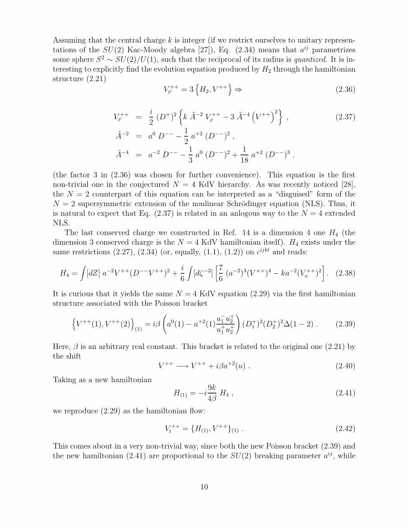
Assuming that the central charge k is integer (if we restrict ourselves to unitary represen-tations of the SU(2) Kac-Moody algebra [27]), Eq. (2.34) means that aij parametrizessome sphere S2 ∼ SU(2)/U(1), such that the reciprocal of its radius is quantized. It is in-teresting to explicitly find the evolution equation produced by H2 through the hamiltonianstructure (2.21)

V ++t′ = 3

{

H2, V++}

⇒ (2.36)

V ++t′ =

i

2(D+)2

{

k A−2 V ++x − 3 A−4

(

V ++)2}

, (2.37)

A−2 = a0 D−− − 1

2a+2 (D−−)2 ,

A−4 = a−2 D−− − 1

3a0 (D−−)2 +

1

18a+2 (D−−)3 .

(the factor 3 in (2.36) was chosen for further convenience). This equation is the firstnon-trivial one in the conjectured N = 4 KdV hierarchy. As was recently noticed [28],the N = 2 counterpart of this equation can be interpreted as a “disguised” form of theN = 2 supersymmetric extension of the nonlinear Schrodinger equation (NLS). Thus, itis natural to expect that Eq. (2.37) is related in an anlogous way to the N = 4 extendedNLS.

The last conserved charge we constructed in Ref. 14 is a dimension 4 one H4 (thedimension 3 conserved charge is the N = 4 KdV hamiltonian itself). H4 exists under thesame restrictions (2.27), (2.34) (or, equally, (1.1), (1.2)) on cijkl and reads:

H4 =∫

[dZ] a−2V ++(D−−V ++)2 +i

6

∫

[dζ−2][

7

6(a−2)3(V ++)4 − ka−2(V ++

x )2]

. (2.38)

It is curious that it yields the same N = 4 KdV equation (2.29) via the first hamiltonianstructure associated with the Poisson bracket

{

V ++(1), V ++(2)}

(1)= iβ

(

a0(1) − a+2(1)u−

1 u+2

u+1 u+

2

)

(D+1 )2(D+

2 )2∆(1 − 2) . (2.39)

Here, β is an arbitrary real constant. This bracket is related to the original one (2.21) bythe shift

V ++ −→ V ++ + iβa+2(u) . (2.40)

Taking as a new hamiltonian

H(1) = −i9k

4βH4 , (2.41)

we reproduce (2.29) as the hamiltonian flow:

V ++t = {H(1), V

++}(1) . (2.42)

This comes about in a very non-trivial way, since both the new Poisson bracket (2.39) andthe new hamiltonian (2.41) are proportional to the SU(2) breaking parameter aij , while

10

the super KdV equation (2.29) includes terms containing no dependence on aij . The keypoint is that these terms appear in (2.42) multiplied by the factor

− k

10s = − k

20aijaij ,

which is independent of harmonic coordinates u± and is constrained to be 1 from thecondition (2.34).

Thus the conditions (2.27) and (2.34) ((1.1), (1.2)) are necessary not only for theexistence of the first non-trivial conservation laws for Eq. (2.29), but also for it to bebi-hamiltonian. This property persists for the evolution equations associated with otherconserved charges. For instance, with respect to the structure (2.39) Eq. (2.37) with aik

constrained by (1.2) has H3 as the hamiltonian.The presence of the bi-hamiltonian structure and the existence of non-trivial conserved

charges are indications that N = 4 KdV equation (2.29) with the restrictions (2.27),(2.34) ((1.1), (1.2)) is integrable, i.e. gives rise to a whole N = 4 super KdV hierarchy.Clearly, in order to prove this, one should, before all, either find the relevant Lax pairor prove the existence of an infinite number of conserved charges of the type given above(e.g., by employing recursion relations implied by the bi-hamiltonian property [1, 11]).Unfortunately, at present it is a very non-trivial and technically complicated problem toanalyse these issues in full generality in the framework of harmonic superspace. Even thedirect construction of the next, dimension 5 charge H5, turned out to be too intricate. InSec. III we will reformulate N = 4 KdV in N = 2 superspace where powerful computermethods for such calculations have been developed. One thing which can be proven in arelatively simple way in the framework of the HSS formalism is that Eq. (2.27) (Eq. (1.1))is a necessary condition for the existence of higher-order conserved charges for (2.29). Weend the present Section with the proof.

First of all, it is clear that after the reduction to N = 2 such charges should becomethose of the integrable N = 2 super KdV equations (see Sec. III for details of thisreduction). Any such charge of dimension, say, l is known to contain in the integrand aterm ∼ V l, where V is the N = 2 super KdV superfield (N = 2 superconformal stress-tensor) [8, 9]. These terms can only be obtained by reduction of analytic integrals of theform

∼∫

[dζ−2] b−2(l−1) (V ++)l , (2.43)

whereb−2(l−1) = bi1...i2(l−1) u−

i1...u−

i2(l−1). (2.44)

If the corresponding charge is to be conserved, the highest order contribution to the timederivative of (2.43) (coming from the 3-d order term in the r.h.s. of (2.29)) should vanishseparately. A simple analysis shows that it is possible if and only if

b−2(l−1) ∼ (a−2)l−1 , c−4 = (a−2)2 . (2.45)

Note that in our previous paper [14] an erroneous statement that this condition is neces-sary only for l = 2n was made.

11

3 N=4 KdV in N=2 superspace

3.1. N=4 KdV and N=4 SU(2) SCA in ordinary N=4 superspace. We firstrewrite Eq. (2.29) in ordinary N = 4 superspace, where it is expressed as an equationfor the superfield V ij(Z) constrained by Eqs. (2.2). A straightforward calculation, thatmakes use of the identities given in Appendix A, yields

V ijt =

{

−1

2k V ij

xx − 2 V (ilx V

j)l +

2i

3TV ij − 4i

9ξ(i ξj) − 3

10

(

cklf(i VklVj)f

)

x

+3

10k cklf(i Vkl xV

j)f − i

10k cijkl

(

TVkl +4

3ξ(kξl)

)}

x

− 3

10cklfg VklVfgV

ijx

−3

5cklfg Vkl

(

V if V j

g

)

x− i

5cklf(i

(

Bj)k Vlf + V

j)k Blf

)

. (3.1)

Here,

Bij ≡ TV ij +8

3ξ(iξj) , (3.2)

the irreducible superfield projections ξk, ξl, T were defined in (2.4) and the subscript“x” corresponds as before to x -derivative. We have verified that both sides of Eq. (3.1)respect the constraints (2.2).

It is also straightforward to rewrite the Poisson bracket (2.21) in ordinary N = 4superspace

{

V ij(Z1), Vkl(Z2)

}

= −D(ij|kl) ∆(1 − 2) , (3.3)

D(ij|kl) =1

4

{[

i V ik Djl ∂ +1

3V ik ǫjl D4 +

i

2∂V kl Dij

+1

6

(

ξk ǫilD2 Dj + ξk ǫilD2 Dj)

+i

4k(

ǫjl Dik ∂2 − i

3ǫik ǫjl D4 ∂

)]

+ (k ↔ l)}

+ (i ↔ j) . (3.4)

HereDij ≡ D(iDj) , D2 ≡ DiDi , D2 ≡ DiD

i , D4 ≡ DijDij , (3.5)

and the differential operator (3.4) is evaluated at the point Z2.The N = 4 KdV hamiltonian (2.26) and the other conserved charges presented in the

previous Section can also be appropriately rewritten. However, it is not very enlighteningto do so, because, as was already said above, only those pieces of these charges which livein the whole harmonic superspace retain a manifestly supersymmetric form after passingto the standard N = 4 superspace (e.g., the integrand in the first term in (2.26) becomes∼ V ijVij). The ordinary N = 4 superspace form of the analytic harmonic superspacepieces explicitly includes θs. Below we will rewrite these conserved quantities via N = 2superfields, so that both kinds of terms will be represented as integrals over the sameN = 2 superspace without explicit θs in the integrands.

3.2. From N=4 to N=2. To make a reduction to N = 2 superspace, we split theN = 4, 1D superspace (2.1) as follows

{ZM} = (x, θ, θ) ⊗ (η, η) ≡ {Zµ} ⊗ (η, η) (3.6)

12

withθ ≡ θ1 , θ ≡ θ1 , η ≡ θ2 , η ≡ θ2 . (3.7)

We also split the set of covariant spinor derivatives into those acting in N = 2 SS {Zµ}and those acting on the extra spinor coordinates η, η

D1 ≡ D , D1 ≡ D, D2 ≡ d , D2 = d ,

{D, D} = i∂ , {d, d} = i∂ , (3.8)

(all other anticommutators are vanishing). Then we put the constraints (2.2) into theform

DV 22 = 0 , dV 11 = 0 , dV 12 =1

2DV 11 , dV 22 = 2DV 12 , (3.9)

DV 11 = 0 , dV 22 = 0 , dV 12 = −1

2DV 22 , dV 11 = −2DV 12 . (3.10)

The first equations in the sets (3.9) and (3.10) are most essential. They tell us that thesuperfields V 11 and V 22 = (V 11)† are chiral and anti-chiral in the N = 2 superspace. Theremainder of constraints and their consequences

ddV 12 = DDV 12 , ddV 11 = iV 11x , ddV 22 = iV 22

x (3.11)

serve to express all the coefficient N = 2 superfields in the η, η expansion of V 12, V 11 andV 22 in terms of spinor and ordinary derivatives of the lowest order N = 2 superfields

V (Zµ) ≡ V 12(ZM)|η=0 , Φ(Zµ) ≡ V 11(ZM)|η=0 , Φ(Zµ) ≡ V 22(ZM)|η=0 (3.12)

DΦ = 0 , DΦ = 0 . (3.13)

Note that V (Zµ) is not constrained by (3.9), (3.10).Thus, by going to N = 2 superspace we have explicitly solved the constraints (2.2) in

terms of an unconstrained N = 2 superfield V and a pair of conjugate chiral and anti-chiral N = 2 superfields Φ, Φ. Now it is clear how to obtain the N = 2 superfield formof Eq. (3.1). Its r.h.s obeys the same constraints (2.2) as the l.h.s, so one should expressall the N = 4 spinor derivatives in the former through N = 2 spinor derivatives, by usingthe constraints in the form (3.9), (3.10). Then one puts η = η = 0 in both sides of theequations obtained. Some useful relations are

ξ1 = −3

2DV 11 , ξ2 = −3 DV 12 , ξ1 = −3 DV 12 ,

ξ2 = −3

2DV 22 , T = 3 [ D, D ] V 12 . (3.14)

The last step needed to put N = 4 KdV in a convenient N = 2 superfield form consistsof choosing an appropriate frame with respect to the global SU(2) that acts on both thedoublet indices in (3.1) and the doublet indices of the N = 4 superspace grassmanncoordinates. It is easy to show that this frame can always be chosen so that only two realcomponents in the SU(2) breaking tensor ciklj are non-zero

c1212 ≡ 5

6a , c1111 = c2222 ≡ 5

6b , c1112 = c2221 = 0 (3.15)

13

(the numerical factors were introduced for further convenience). Note that this is still trueif cijkl is bilinear in the constant vector aik in accord with Eq. (2.27). In this importantcase

cijkl =1

3(aijakl + aikajl + ailajk) . (3.16)

For three independent SU(2) fixations of aik

(a) a11 = a22 = 0 , a12 6= 0; (b) a12 = 0 , a11 = a22 6= 0;

(c) a12 = 0 , a11 = −a22 6= 0 , (3.17)

the components of cijkl satisfy (3.15). The values of a and b are given by

(a) a =4

5a12a12 , b = 0; (b) a =

2

5a11a11 , b = 3 a

(c) a = −2

5a11a22 , b = −3 a . (3.18)

As we will see below, only these choices of the SU(2) frame allow an unambiguous reduc-tion to N = 2 KdV.

The whole tensor cijkl (or aik in the case (2.27), (3.16)) can be restored by an appro-priate SU(2) rotation. It is instructive to describe how these SU(2) rotations, which aremanifest in the original N = 4 superspace, are realized on N = 2 superfields V , Φ, Φ

δ∗V = −λ0

(

θ∂

∂θ− θ

∂

∂θ

)

V + λ+ [Φ + D (θΦ)] − λ−

[

Φ − D ( θΦ )]

,

δ∗Φ = λ0

(

2 − θ∂

∂θ+ θ

∂

∂θ

)

Φ + λ−D ( θV ) ,

δ∗Φ = λ0

(

−2 − θ∂

∂θ+ θ

∂

∂θ

)

Φ + λ+D ( θV ) . (3.19)

For completeness, we also give the transformation properties of the superfields under thesecond complex supersymmetry, implicit in the N = 2 superfield notation

δ∗V =1

2ǫ2DΦ +

1

2ǫ2DΦ ,

δ∗Φ = 2 ǫ2DV , δ∗Φ = 2 ǫ2DV . (3.20)

After these preparatory steps and choosing, for convenience, k = 2 henceforth, wededuce the N = 4 SU(2) KdV equation in a N = 2 superfield form as the followingsystem of coupled evolution equations

Vt = −Vxxx + 3i([

D, D]

V V)

x− i

2(1 − a)

([

D, D]

V 2)

x− 3a VxV

2

+1

4(a − 4)

(

ΦxΦ − ΦxΦ)

x+

i

2(a − 1)

(

DΦDΦ)

x− 3

2a(

V ΦΦ)

x

+1

8b(

Φ2 − Φ2)

xx− 3

4b[

V(

Φ2 + Φ2)]

x+

i

2b[

D, D] [

V(

Φ2 − Φ2)]

(3.21)

14

Φt = −Φxxx −5

4b ΦxΦ

2 − D [6i (DV Φ)x − i (a + 2) D (V Φ)x]

+DD[

3i a(

V 2Φ +1

4Φ2Φ

)

+ i b(

V Φ)

x+ i b

(

V 2Φ +1

4Φ2Φ

)]

(3.22)

Φt = −Φxxx −5

4b ΦxΦ

2 + D[

6i(

DV Φ)

x− i (a + 2) D

(

V Φ)

x

]

+DD[

3i a(

V 2Φ +1

4Φ2Φ

)

− i b (V Φ)x + i b(

V 2Φ +1

4Φ2Φ

)]

. (3.23)

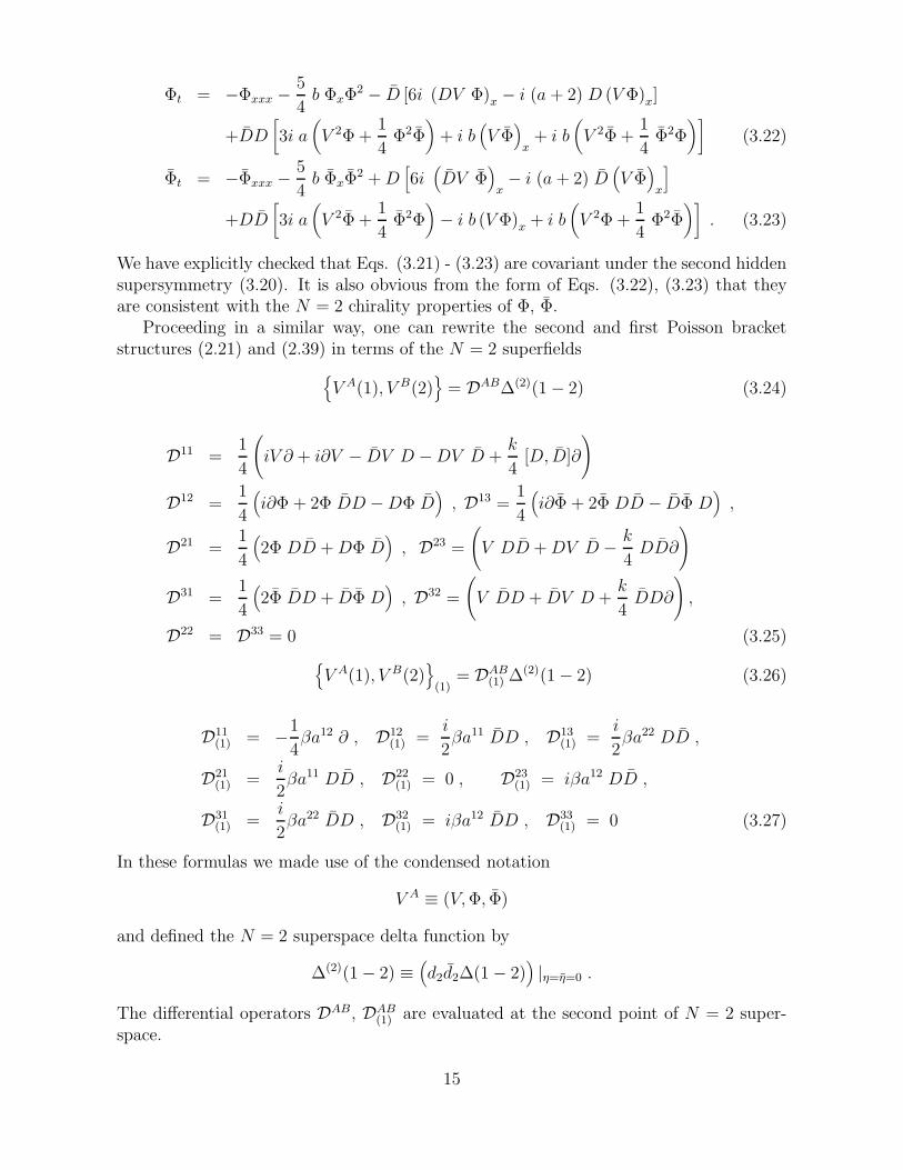
We have explicitly checked that Eqs. (3.21) - (3.23) are covariant under the second hiddensupersymmetry (3.20). It is also obvious from the form of Eqs. (3.22), (3.23) that theyare consistent with the N = 2 chirality properties of Φ, Φ.

Proceeding in a similar way, one can rewrite the second and first Poisson bracketstructures (2.21) and (2.39) in terms of the N = 2 superfields

{

V A(1), V B(2)}

= DAB∆(2)(1 − 2) (3.24)

D11 =1

4

(

iV ∂ + i∂V − DV D − DV D +k

4[D, D]∂

)

D12 =1

4

(

i∂Φ + 2Φ DD − DΦ D)

, D13 =1

4

(

i∂Φ + 2Φ DD − DΦ D)

,

D21 =1

4

(

2Φ DD + DΦ D)

, D23 =

(

V DD + DV D − k

4DD∂

)

D31 =1

4

(

2Φ DD + DΦ D)

, D32 =

(

V DD + DV D +k

4DD∂

)

,

D22 = D33 = 0 (3.25)

{

V A(1), V B(2)}

(1)= DAB

(1) ∆(2)(1 − 2) (3.26)

D11(1) = −1

4βa12 ∂ , D12

(1) =i

2βa11 DD , D13

(1) =i

2βa22 DD ,

D21(1) =

i

2βa11 DD , D22

(1) = 0 , D23(1) = iβa12 DD ,

D31(1) =

i

2βa22 DD , D32

(1) = iβa12 DD , D33(1) = 0 (3.27)

In these formulas we made use of the condensed notation

V A ≡ (V, Φ, Φ)

and defined the N = 2 superspace delta function by

∆(2)(1 − 2) ≡(

d2d2∆(1 − 2))

|η=η=0 .

The differential operators DAB, DAB(1) are evaluated at the second point of N = 2 super-

space.

15

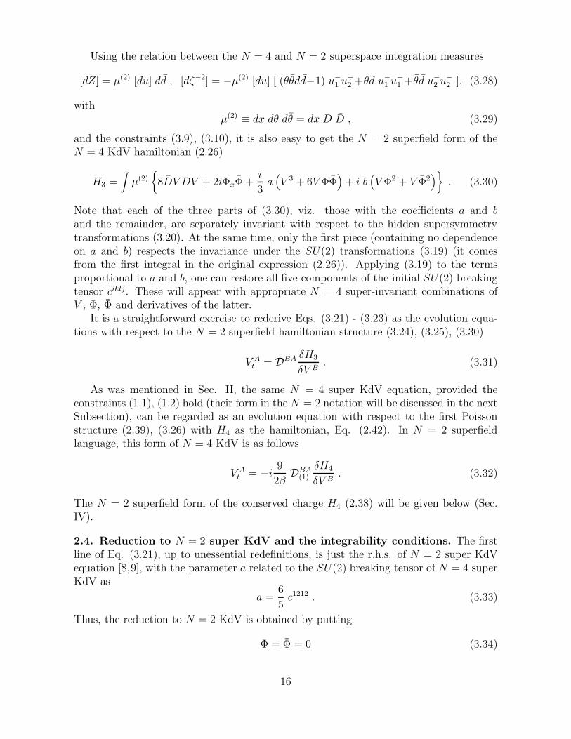
Using the relation between the N = 4 and N = 2 superspace integration measures

[dZ] = µ(2) [du] dd , [dζ−2] = −µ(2) [du] [ (θθdd−1) u−1 u−

2 +θd u−1 u−

1 +θd u−2 u−

2 ], (3.28)

withµ(2) ≡ dx dθ dθ = dx D D , (3.29)

and the constraints (3.9), (3.10), it is also easy to get the N = 2 superfield form of theN = 4 KdV hamiltonian (2.26)

H3 =∫

µ(2){

8DV DV + 2iΦxΦ +i

3a(

V 3 + 6V ΦΦ)

+ i b(

V Φ2 + V Φ2)

}

. (3.30)

Note that each of the three parts of (3.30), viz. those with the coefficients a and band the remainder, are separately invariant with respect to the hidden supersymmetrytransformations (3.20). At the same time, only the first piece (containing no dependenceon a and b) respects the invariance under the SU(2) transformations (3.19) (it comesfrom the first integral in the original expression (2.26)). Applying (3.19) to the termsproportional to a and b, one can restore all five components of the initial SU(2) breakingtensor ciklj. These will appear with appropriate N = 4 super-invariant combinations ofV , Φ, Φ and derivatives of the latter.

It is a straightforward exercise to rederive Eqs. (3.21) - (3.23) as the evolution equa-tions with respect to the N = 2 superfield hamiltonian structure (3.24), (3.25), (3.30)

V At = DBA δH3

δV B. (3.31)

As was mentioned in Sec. II, the same N = 4 super KdV equation, provided theconstraints (1.1), (1.2) hold (their form in the N = 2 notation will be discussed in the nextSubsection), can be regarded as an evolution equation with respect to the first Poissonstructure (2.39), (3.26) with H4 as the hamiltonian, Eq. (2.42). In N = 2 superfieldlanguage, this form of N = 4 KdV is as follows

V At = −i

9

2βDBA

(1)

δH4

δV B. (3.32)

The N = 2 superfield form of the conserved charge H4 (2.38) will be given below (Sec.IV).

2.4. Reduction to N = 2 super KdV and the integrability conditions. The firstline of Eq. (3.21), up to unessential redefinitions, is just the r.h.s. of N = 2 super KdVequation [8,9], with the parameter a related to the SU(2) breaking tensor of N = 4 superKdV as

a =6

5c1212 . (3.33)

Thus, the reduction to N = 2 KdV is obtained by putting

Φ = Φ = 0 (3.34)

16

in Eqs. (3.21) - (3.23). As a result of the reduction, one gets

Vt = −Vxxx + 3i([

D, D]

V V)

x− i

2(1 − a)

([

D, D]

V 2)

x− 3a VxV

2 . (3.35)

This equation is related to the standard form of N = 2 KdV equation given in Refs. 8and 9 via the redefinitions

V = V , ∂x = i∂x , ∂t = −i∂t , D =1

2(D1 + iD2) , D = −1

2(D1 − iD2) ,

D 21 = D 2

2 = ∂x . (3.36)

We should point out that the above reduction is consistent because Eqs. (3.22) and(3.23) are homogeneous in Φ, Φ and, for this reason, condition (3.34) together with Eq.(3.35) yield a particular solution of the original set (3.21) - (3.23). The superfield Vsatisfies Eq. (3.35) and is unconstrained otherwise. All the conserved charges of N = 4KdV become conserved charges of N = 2 KdV in the reduction limit.

This is not the case for any other choice of the SU(2) frame beside those leadingto (3.15). This is because for non-zero c1112 and c2221 there appear extra pieces in theequations for Φ, Φ, that do not vanish after the reduction (3.34). For example, for Eq.(3.22) these pieces are as follows

△Φt = −2

5i c1112 DD

[

3 V Vx + 4 V 3]

. (3.37)

In this case, the reduction to N = 2 KdV is inconsistent, because the superfield V becomesconstrained in the N = 2 KdV limit (the r.h.s. of Eq. (3.37) should vanish after imposing(3.34)). To avoid confusion, we mention that the systems associated with these otherchoices of the SU(2) frame are simply other “SU(2) gauges” of the same N = 4 superKdV equation. They can be rotated into Eqs. (3.21) - (3.23) by an appropriate SU(2)transformation. Only in the N = 2 KdV limit, where SU(2) covariance gets broken,different choices of the SU(2) frame turn out to lead to inequivalent systems.

Now let us see which values of a correspond to the restrictions (2.27), (2.34) (or (1.1),(1.2)) that are required for N = 4 KdV to be integrable. According to the reasoningsjust mentioned, only three directions of the SU(2) vector aij , summarized in Eq. (3.17),allow for an unambigous reduction to N = 2 super KdV. Indeed, only under this choicethe components

c1112 = −(c2221)† = a11a12

are zero. Then, substituting the relations (3.17) into (2.34) we find three cases for whichN = 4 super KdV in the N = 2 superfield form (3.21) - (3.23) is expected to be integrable

(a) a = 4, b = 0; (b) a = −2, b = −6; (c) a = −2, b = 6 . (3.38)

In the full N = 4 case these possibilities are all equivalent since they are related bySU(2) rotations. Nevertheless, they yield inequivalent systems upon the reduction (3.34).Remarkably, these are precisely two integrable N = 2 KdV hierarchies, the a = 4 and

a = −2 N = 2 KdVs [8, 9].

17

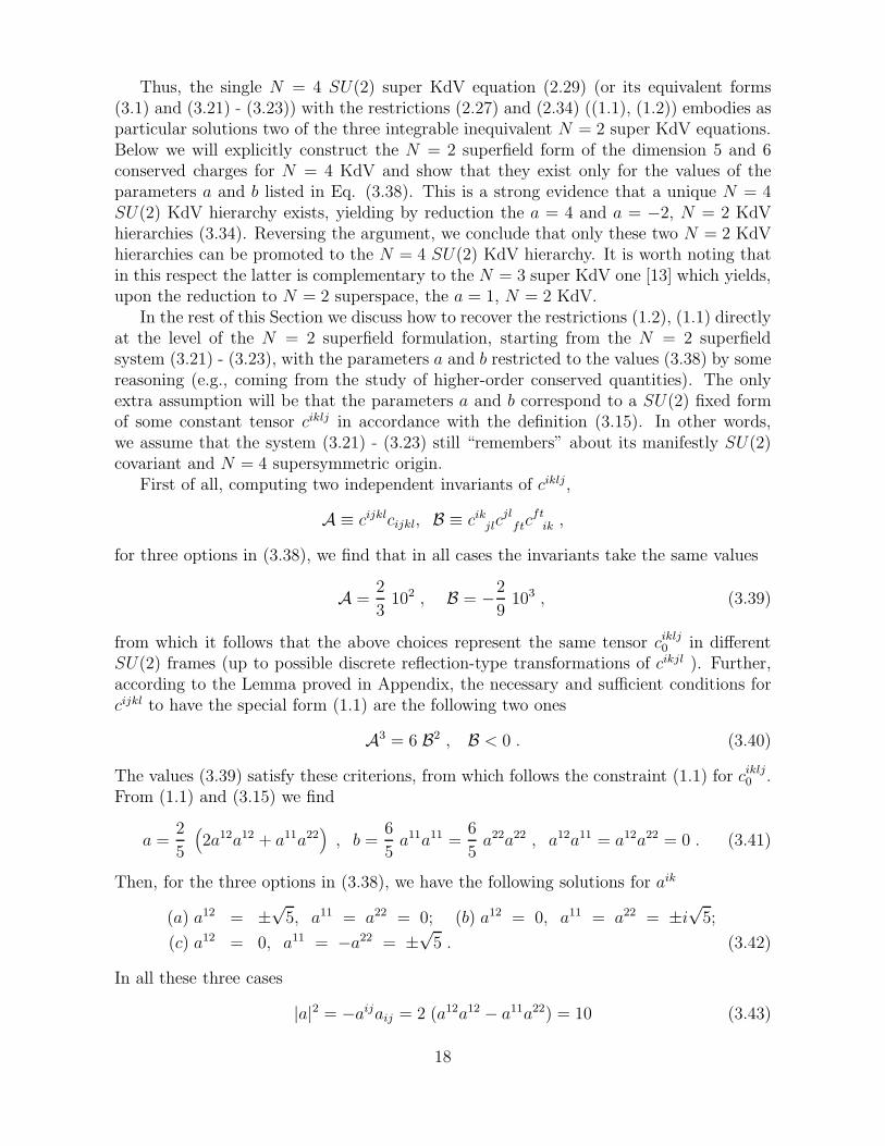
Thus, the single N = 4 SU(2) super KdV equation (2.29) (or its equivalent forms(3.1) and (3.21) - (3.23)) with the restrictions (2.27) and (2.34) ((1.1), (1.2)) embodies asparticular solutions two of the three integrable inequivalent N = 2 super KdV equations.Below we will explicitly construct the N = 2 superfield form of the dimension 5 and 6conserved charges for N = 4 KdV and show that they exist only for the values of theparameters a and b listed in Eq. (3.38). This is a strong evidence that a unique N = 4SU(2) KdV hierarchy exists, yielding by reduction the a = 4 and a = −2, N = 2 KdVhierarchies (3.34). Reversing the argument, we conclude that only these two N = 2 KdVhierarchies can be promoted to the N = 4 SU(2) KdV hierarchy. It is worth noting thatin this respect the latter is complementary to the N = 3 super KdV one [13] which yields,upon the reduction to N = 2 superspace, the a = 1, N = 2 KdV.

In the rest of this Section we discuss how to recover the restrictions (1.2), (1.1) directlyat the level of the N = 2 superfield formulation, starting from the N = 2 superfieldsystem (3.21) - (3.23), with the parameters a and b restricted to the values (3.38) by somereasoning (e.g., coming from the study of higher-order conserved quantities). The onlyextra assumption will be that the parameters a and b correspond to a SU(2) fixed formof some constant tensor ciklj in accordance with the definition (3.15). In other words,we assume that the system (3.21) - (3.23) still “remembers” about its manifestly SU(2)covariant and N = 4 supersymmetric origin.

First of all, computing two independent invariants of ciklj,

A ≡ cijklcijkl, B ≡ cikjlc

jlftc

ftik ,

for three options in (3.38), we find that in all cases the invariants take the same values

A =2

3102 , B = −2

9103 , (3.39)

from which it follows that the above choices represent the same tensor ciklj0 in different

SU(2) frames (up to possible discrete reflection-type transformations of cikjl ). Further,according to the Lemma proved in Appendix, the necessary and sufficient conditions forcijkl to have the special form (1.1) are the following two ones

A3 = 6 B2 , B < 0 . (3.40)

The values (3.39) satisfy these criterions, from which follows the constraint (1.1) for ciklj0 .

From (1.1) and (3.15) we find

a =2

5

(

2a12a12 + a11a22)

, b =6

5a11a11 =

6

5a22a22 , a12a11 = a12a22 = 0 . (3.41)

Then, for the three options in (3.38), we have the following solutions for aik

(a) a12 = ±√

5, a11 = a22 = 0; (b) a12 = 0, a11 = a22 = ±i√

5;

(c) a12 = 0, a11 = −a22 = ±√

5 . (3.42)

In all these three cases

|a|2 = −aijaij = 2 (a12a12 − a11a22) = 10 (3.43)

18

that is precisely the constraint (1.2) at k = 2. Note that the reconstruction of the vectoraik from the known cijkl

0 is unique modulo some reflections of aik, as is seen from theexplicit solution (3.42).

Finally, we note that, when analyzing the integrability properties of N = 4 super KdVin the N = 2 superfield formulation, we actually do not need to keep track of all thesesubtleties concerning the relation between cijkl and aik, etc. One can forget about theN = 4 superfield origin of the system (3.21) - (3.23) and view it as some two-parameterextension of N = 2 KdV equation. Then the specific values (3.38) of the parameters a andb come out as the values at which this system possesses higher-order conserved chargesand is bi-hamiltonian (see next Section). Of course, in order to see that the three optionsin Eq. (3.38) are actually equivalent to each other, one should take into account the factthat the system (3.21) - (3.23) respects a hidden SU(2) symmetry, or, eqivalently, admitsa manifestly N = 4 supersymmetric and SU(2) covariant description discussed in Sec. II.The above discussion was aimed just at carefully clarifying the links between this latterdescription and the N = 2 superfield one.

4 Conserved charges in the N=2 superfield formula-

tion

In this Section we put into an N = 2 superfield form all the N = 4 super KdV conservedcharges given in Ref. 14 and Sec. II and present two new ones: H5 and H6. We find thatall these charges exist under the same restrictions (3.38) which, as was discussed in theend of previous Section, actually amount to the original constraints (1.1), (1.2).

4.1 The charges H1 and H2. In order to find the N = 2 superfield representation of theconserved charges initially written as integrals over N = 4 HSS and its analytic subspace,we proceed in the same way that was used to get the N = 2 superfield form of H3, Eq.(3.30). Namely, we make use of the relations (3.28) and (3.9), (3.10) and do the harmonicintegrals in the end.

The charge H1 (2.32) is of the same form as in the N = 2 KdV case

H1 = −2∫

µ(2)V . (4.1)

Starting with H2, non-trivial contributions of the superfields Φ, Φ come out

H2 =4i

3

∫

µ(2){

a12(

V 2 +1

2ΦΦ

)

− a11 V Φ − a22 V Φ}

. (4.2)

Like in H3, three terms in (4.2) are separately invariant under the hidden supersymmetry(3.20) but are mixed by the SU(2) transformations (3.19). Assuming for the moment thatthe coefficients aik are arbitrary, we have checked the conservation of (4.2) with respect toEqs. (3.21) - (3.23), both “by hand” and using the computer, and found (H2)t to vanishunder the following conditions

(a) a = 4 , b = 0 , a12 6= 0 , a11 = a22 = 0 ;

(b) a = −2 , b = −6 , a12 = 0 , a11 = a22 6= 0 ;

(c) a = −2 , b = 6 , a12 = 0 , a11 = −a22 6= 0 . (4.3)

19

Keeping in mind the discussion in the end of previous Section (see Eqs. (3.42)), thesesolutions, up to relative scaling factors, precisely correspond to the conditions (1.1), (1.2)found from the computations in HSS.

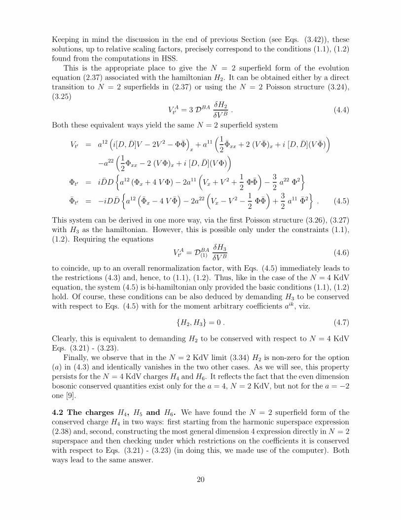
This is the appropriate place to give the N = 2 superfield form of the evolutionequation (2.37) associated with the hamiltonian H2. It can be obtained either by a directtransition to N = 2 superfields in (2.37) or using the N = 2 Poisson structure (3.24),(3.25)

V At′ = 3 DBA δH2

δV B. (4.4)

Both these equivalent ways yield the same N = 2 superfield system

Vt′ = a12(

i[D, D]V − 2V 2 − ΦΦ)

x+ a11

(

1

2Φxx + 2 (V Φ)x + i [D, D](V Φ)

)

−a22(

1

2Φxx − 2 (V Φ)x + i [D, D](V Φ)

)

Φt′ = iDD{

a12 (Φx + 4 V Φ) − 2a11(

Vx + V 2 +1

2ΦΦ

)

− 3

2a22 Φ2

}

Φt′ = −iDD{

a12(

Φx − 4 V Φ)

− 2a22(

Vx − V 2 − 1

2ΦΦ

)

+3

2a11 Φ2

}

. (4.5)

This system can be derived in one more way, via the first Poisson structure (3.26), (3.27)with H3 as the hamiltonian. However, this is possible only under the constraints (1.1),(1.2). Requiring the equations

V At′ = DBA

(1)

δH3

δV B(4.6)

to coincide, up to an overall renormalization factor, with Eqs. (4.5) immediately leads tothe restrictions (4.3) and, hence, to (1.1), (1.2). Thus, like in the case of the N = 4 KdVequation, the system (4.5) is bi-hamiltonian only provided the basic conditions (1.1), (1.2)hold. Of course, these conditions can be also deduced by demanding H3 to be conservedwith respect to Eqs. (4.5) with for the moment arbitrary coefficients aik, viz.

{H2, H3} = 0 . (4.7)

Clearly, this is equivalent to demanding H2 to be conserved with respect to N = 4 KdVEqs. (3.21) - (3.23).

Finally, we observe that in the N = 2 KdV limit (3.34) H2 is non-zero for the option(a) in (4.3) and identically vanishes in the two other cases. As we will see, this propertypersists for the N = 4 KdV charges H4 and H6. It reflects the fact that the even dimensionbosonic conserved quantities exist only for the a = 4, N = 2 KdV, but not for the a = −2one [9].

4.2 The charges H4, H5 and H6. We have found the N = 2 superfield form of theconserved charge H4 in two ways: first starting from the harmonic superspace expression(2.38) and, second, constructing the most general dimension 4 expression directly in N = 2superspace and then checking under which restrictions on the coefficients it is conservedwith respect to Eqs. (3.21) - (3.23) (in doing this, we made use of the computer). Bothways lead to the same answer.

20

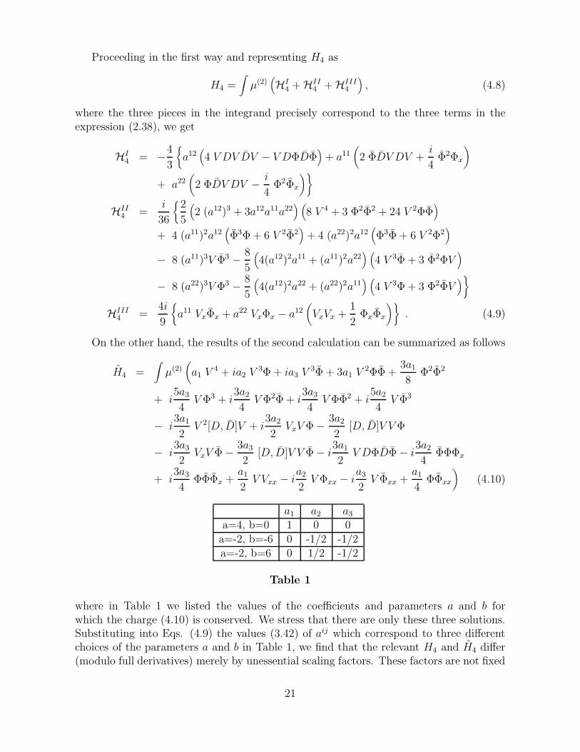
Proceeding in the first way and representing H4 as

H4 =∫

µ(2)(

HI4 + HII

4 + HIII4

)

, (4.8)

where the three pieces in the integrand precisely correspond to the three terms in theexpression (2.38), we get

HI4 = −4

3

{

a12(

4 V DV DV − V DΦDΦ)

+ a11(

2 ΦDV DV +i

4Φ2Φx

)

+ a22(

2 ΦDV DV − i

4Φ2Φx

)}

HII4 =

i

36

{

2

5

(

2 (a12)3 + 3a12a11a22) (

8 V 4 + 3 Φ2Φ2 + 24 V 2ΦΦ)

+ 4 (a11)2a12(

Φ3Φ + 6 V 2Φ2)

+ 4 (a22)2a12(

Φ3Φ + 6 V 2Φ2)

− 8 (a11)3V Φ3 − 8

5

(

4(a12)2a11 + (a11)2a22) (

4 V 3Φ + 3 Φ2ΦV)

− 8 (a22)3V Φ3 − 8

5

(

4(a12)2a22 + (a22)2a11) (

4 V 3Φ + 3 Φ2ΦV)

}

HIII4 =

4i

9

{

a11 VxΦx + a22 VxΦx − a12(

VxVx +1

2ΦxΦx

)}

. (4.9)

On the other hand, the results of the second calculation can be summarized as follows

H4 =∫

µ(2)(

a1 V 4 + ia2 V 3Φ + ia3 V 3Φ + 3a1 V 2ΦΦ +3a1

8Φ2Φ2

+ i5a3

4V Φ3 + i

3a2

4V Φ2Φ + i

3a3

4V ΦΦ2 + i

5a2

4V Φ3

− i3a1

2V 2[D, D]V + i

3a2

2VxV Φ − 3a2

2[D, D]V V Φ

− i3a3

2VxV Φ − 3a3

2[D, D]V V Φ − i

3a1

2V DΦDΦ − i

3a2

4ΦΦΦx

+ i3a3

4ΦΦΦx +

a1

2V Vxx − i

a2

2V Φxx − i

a3

2V Φxx +

a1

4ΦΦxx

)

(4.10)

a1 a2 a3

a=4, b=0 1 0 0a=-2, b=-6 0 -1/2 -1/2a=-2, b=6 0 1/2 -1/2

Table 1

where in Table 1 we listed the values of the coefficients and parameters a and b forwhich the charge (4.10) is conserved. We stress that there are only these three solutions.Substituting into Eqs. (4.9) the values (3.42) of aij which correspond to three differentchoices of the parameters a and b in Table 1, we find that the relevant H4 and H4 differ(modulo full derivatives) merely by unessential scaling factors. These factors are not fixed

21

by requiring the conservation of the N = 4 KdV charges in the N = 2 superfield formalismand can always be chosen so as to achieve the full coincidence between H4 and H4. Thus,the independent N = 2 superfield calculation entirely confirms the conclusions about H4

made in our previous paper [14] in the framework of the HSS formalism.Having at our disposal the explicit N = 2 superfield form of H4 we can check the first

hamiltonian structure representation (3.32) for N = 4 KdV system (3.21) - (3.23). Likein the case of the set (4.5), the necessary conditions for the existence of such a represen-tation are the above constraints on the parameters a and b. Actually, an alternative andtechnically more simple way to obtain (4.10) with the coefficients from Table 1 is to startfrom the most general N = 2 superfield expression for H4 and to require it to reproduceEqs. (3.21) - (3.23) via the Poisson structure (3.26), (3.27).

Note that for the second and third lines in Table 1, the charge H4 identically vanishesin the N = 2 KdV limit (3.34) in accordance with the absence of the even dimensionbosonic conserved charges for the a = −2, N = 2 KdV hierarchy.

Let us now present the conserved charge H5. As was already mentioned, it is a verycomplicated technical problem to construct it directly in the harmonic superspace for-malism. This becomes feasible in the N = 2 superfield approach due to the possibility touse a computer. We start from the most general dimension 5 N = 2 superfield expres-sion for H5 with undetermined coefficients and then examined the restrictions imposedon these coefficients by the conservation condition (H5)t = 0. Like in the case of thelower-dimension charges, we have found only three solutions

H5 =∫

µ(2){

i

4ΦΦxxx − V [D, D]Vxx − ia1V

2Vxx + 2iV [D, D]V [D, D]V

+ ia2V ΦΦxx +ia2

2V ΦxΦx + ia3V ΦxxΦ + ia4V ΦxΦx + ia3V ΦΦxx

− 2V DΦxDΦ + 2V DΦDΦx + ia2V ΦΦxx +ia2

2V ΦxΦx

+ 2a4V3[D, D]V +

3ia2

2V 2ΦΦx +

3a2

2V [D, D]V Φ2 +

3ia4

2V 2ΦxΦ

− 3ia4

2V 2ΦΦx + 3a4V [D, D]V ΦΦ − 12DV DV ΦΦ − 3ia2

2V 2ΦΦx

+3a2

2V [D, D]V Φ2 − ia2

4ΦxΦ

3 − 3ia3

4Φ2ΦΦx +

ia2

4ΦxΦ

3

− ia5V5 − ia2V

3Φ2 − 5ia5V3ΦΦ − ia2V

3Φ2 − ia6V Φ4

− ia2

2V Φ3Φ − ia7V Φ2Φ2 − ia2

2V ΦΦ3 − ia6V Φ4

}

. (4.11)

a1 a2 a3 a4 a5 a6 a7

a=4, b=0 3 0 -2 -4 16/5 0 6a=-2, b=6 -2 -5 3 1 6/5 35/8 9/4a=-2, b=-6 -2 5 3 1 6/5 35/8 9/4

Table 2

Thus, H5 exists under the same restrictions (3.38) on the N = 4 KdV parameters aand b (or their manifestly SU(2) covariant form (1.1), (1.2)) as in the previous cases. After

22

reduction to N = 2 super KdV by setting Φ = Φ = 0, H5 is reduced to the 5 dimensionconserved charges of the a = 4 and a = −2, N = 2 KdV hierarchies, respectively, for thefirst line and the last two lines in Table 2.

It is interesting to see how this conserved charge looks in the original manifestlyN = 4 supersymmetric formulation. It is a matter of straightforward though somewhatcumbersome computation to find that the following N = 4 superfield expression yields(4.11) after passing to N = 2 superfields and imposing the constraint (1.2)

H5 =1

2

∫

[dZ][

1

4

(

D−−V ++)4

+ i(

D−−V ++)2 (

D−)2

V ++

+15

4(a−2)2

(

D−−V ++)2 (

V ++)2 − 1

2

(

D−−V ++x

)2]

+i

4

∫

[dζ−2][

63

100(a−2)4

(

V ++)5 − 5 (a−2)2

(

V ++x

)2V ++

]

. (4.12)

The last conserved charge we have explicitly constructed is H6. Once again, it existsonly for the above three choices of the N = 4 KdV parameters. We present it here onlyfor the choice a = 4, b = 0 since the expressions for the two other choices are very longand complicated. Of course, they can be obtained from the a = 4, b = 0 expression viafinite SU(2) rotations.

This charge H6 reads

H6 =∫

µ(2){

6 ΦxxxxΦ + 12 V Vxxxx − 240i DVxDVxV − 120i [D, D]VxxV2

+ 60i V DΦDΦxx + 60i V DΦxDΦx + 60i V DΦxxDΦ

− 240i DV DV ΦxΦ − 240i DV DVxΦΦ − 60 [D, D]V [D, D]V ΦΦ

− 120 [D, D]V [D, D]V V 2 + 240i [D, D]V V ΦxΦ + 120i [D, D]V VxΦΦ

+ 120i [D, D]VxV ΦΦ − 15 Φ2(Φx)2 + 30 ΦΦxxΦ

2 + 15 (Φx)2Φ2

+ 240 V 2ΦxxΦ + 120 V 3Vxx + 480 V VxΦxΦ + 360 V VxxΦΦ

+ 180 (Vx)2ΦΦ + 1440i DV DV V ΦΦ − 45i [D, D]V Φ2Φ2

− 720i [D, D]V V 2ΦΦ − 240i [D, D]V V 4 + 90 V Φ2ΦΦx

− 90 V ΦΦxΦ2 + 240 V 3ΦΦx − 240 V 3ΦxΦ + 20 Φ3Φ3

+ 360 V 2Φ2Φ2 + 480 V 4ΦΦ + 64i V 5}

. (4.13)

Finally, we wish to stress that all the conserved charges Hn, n = 1, ...6, are in involutionwith respect to both Poisson brackets

{Hn, Hm} = {Hn, Hm}(1) = 0 . (4.14)

This property can be easily deduced from the bi-hamiltonian nature of the conjecturalN = 4 KdV hierarchy. The bi-hamiltonian structure can be expressed as the followinggeneral recursion relation (up to relative scaling factors between the conserved charges)

DAB δHn

δV A= DAB

(1)

δHn+1

δV A. (4.15)

23

We have explicitly checked (4.15) for all Hn presented above, limiting ourselves, for sim-plicity, to the case a = 4, b = 0 and keeping in mind that the other two integrable casescan be generated from this one by SU(2) transformations (3.19). Actually, as we al-ready mentioned, postulating the relations (4.15) gives an alternative method to constructhigher-order conservation laws, even more simple than the direct method we resorted toin this Section. We do not foresee any reason why the construction procedure of theselaws based on the relations (4.15) should terminate at any finite step. Both the existenceof the non-trivial conserved charges H2, H4, H5 and H6 and the above bi-hamiltonianproperty are strong indications that the N = 4 super KdV equation with the restrictions(1.1), (1.2) produces the whole N = 4 super KdV hierarchy and so is integrable. Inorder to rigorously prove this, it is of primary importance to find the appropriate Laxrepresentation. We believe that in the N = 2 superfield formalism this problem will besimpler than in the harmonic superspace formulation and can be solved along the lines ofRefs. 10, 11 and 28.

5 Conclusion

As the main goal of the present work, we have obtained the N = 4 super KdV equationof Ref. 14 in an N = 2 superfield form and studied the question of its integrability inthis approach. We reproduced the results of Ref. 14 and constructed two new conservedbosonic quantities for N = 4 super KdV, the dimension 5 and 6 ones H5 and H6. Theywere found to exist under the same restrictions on the SU(2) breaking parameters (1.1),(1.2) as the lower dimension charges given in Ref. 14. The bi-hamiltonian structure ofthe N = 4 KdV equation was extended to the whole set of evolution equation associatedwith the hamiltonians Hn that have been constructed. Requiring the existence of thisstructure gives rise to the same conditions (1.1), (1.2) on the parameters. These resultssuggest that the unique integrable N = 4 SU(2) KdV hierarchy exists, with the choice ofthe SU(2) breaking parameters as in Eqs. (1.1), (1.2). The N = 2 superfield formulationallowed us also to show that two inequivalent reductions to N = 2 KdV are possible.They yield, respectively, the integrable a = 4 and a = −2 cases of N = 2 KdV. Thus thesingle N = 4 SU(2) KdV hierarchy incorporates as particular solutions two of the threeN = 2 KdV hierarchies.

Among the problems for future study, besides the construction of a Lax pair repre-sentation for the N = 4 SU(2) KdV, let us mention a generalization to the case of the“large” N = 4 superconformal algebra [25, 26] with the affine subalgebra so(4) × u(1).The related N = 4 super KdV hierarchy is expected to embrace both the N = 4 SU(2)and N = 3 KdV ones as particular cases. Also, it would be interesting to construct gener-alized N = 4 super KdV systems associated with nonlinear W type extensions of N = 4superconformal algebras. One of possible ways to define such extensions was mentionedin Subsec. 2.1.

Acknowledgements

E.I. is grateful to P. Mathieu for useful discussions. He also thanks ENSLAPP, ENS-Lyon,for hospitality extended to him during the course of this work. E.I. and S.K. thank the

24

Russian Foundation of Fundamental Research, grant 93-02-03821, and the InternationalScience Foundation, grant M9T300, for financial support.

Appendix A

In this Appendix we collect a number of useful identities.First of all, we present some consequences of the constraints (2.2) and their harmonic

superspace version (2.10), (2.11):

DiV kl = −1

3

(

ǫikξl + ǫilξk)

, DiV kl =1

3

(

ǫikξl + ǫilξk)

, (A.1)

DiDjV kl = − i

2

(

ǫjkV ilx + ǫjlV ik

x

)

− 1

6

(

ǫilǫjk + ǫikǫjl)

T (A.2)

DiDjV kl = DiDjV kl = 0 , (A.3)

D−V ++ = −2

3ξku+

k , D−V ++ =2

3ξku+

k , (A.4)

(D−)2V ++ = − i

2D−−V ++

x − 1

3T . (A.5)

When deducing Eqs. (2.29) and (2.37) from the harmonic superspace Poisson structure(2.21) and rewriting the latter in ordinary N = 4 superspace, one needs to decomposethe objects given in terms of one set of harmonic variables, say u±

i , over another set,v±

i , using the completeness condition (2.5). The general decomposition formula for someobject bilinear in harmonics,

S++(u) ≡ Siku+i u+

k

(S++ can stand, e.g., for V ++ or (D+)2 = D+D+), is as follows

S++(u) = S++(v)(v−u+)2+1

2(D−−

v )2S++(v)(v+u+)2−D−−v S++(v)(v−u+)(v+u+) . (A.6)

Analogous relations for other harmonic projections of Sik, namely S+− and S−−, can beobtained by applying D−−

u to both sides of Eq. (A.6) and making use of the harmonicdifferentiation rules

D−−u+i = u−

i , D−−u−i = 0 .

Appendix B

In this Appendix we prove the following Lemma.Lemma: Let ciklj be an arbitrary rank 4 symmetric SU(2) spinor subjected to the

reality condition(ciklj)† = ǫii′ǫkk′ǫll′ǫjj′c

i′k′l′j′.

The necessary and sufficient conditions for it to be a square of some real rank 2 symmetricSU(2) spinor aik,

cijkl =1

3

(

aijakl + aikajl + ailajk)

, (aik)† = −ǫilǫkjalj , (B.1)

25

are the following ones

(I) A3 = 6 B2 , (II) B < 0 ;(

A ≡ cijkl cijkl, B ≡ cikjl cjl

ft cftik

)

. (B.2)

Proof: The proof is simpler in the vector notation, with cikjl represented by a realtraceless symmetric rank 2 tensor and aik by a real vector

ciklj ⇒ cµν =1

2cij

kl(σµ)k

i (σν)l

j , aik ⇒ aµ =1√2ai

k(σµ)k

i ; (µ, ν... = 1, 2, 3)

A = cµνcµν , B = −cµνcνρcρµ .

Here, (σµ)lk are Pauli matrices.

In this notation, the relation (B.1) amounts to

cµν = aµaν − 1

3δµν (aρaρ) . (B.3)

Then the necessity of (B.2) immediately follows from computing the invariants A and Bfor the tensor (B.3)

A =2

3(a2)2 , B = −2

9(a2)3 , a2 ≡ aµaµ > 0 .

In order to show that (B.2) is also sufficient for cµν to be representable in the form(B.3), let us go to the frame where cµν is a diagonal traceless matrix with the followingnon-zero entries

c11 = λ1, c22 = λ2, c33 = −(λ1 + λ2) , (B.4)

λ1, λ2 being arbitrary for the moment. After substituting this into the first of conditions(B.2) we get the equation

(λ1 − λ2)2 (λ1 + 2λ2) (2λ1 + λ2) = 0 , (B.5)

which has the following non-zero roots

(a) λ1 = λ2; (b) λ1 = −2λ2; (c) λ2 = −2λ1 . (B.6)

The inequality in (B.2) takes the form

λ1λ2 (λ1 + λ2) < 0 (B.7)

and restricts the solutions (B.6) in the following way

(a) λ1 < 0 , (b) λ1 > 0 , (c) λ1 < 0 . (B.8)

Now it is an elementary exercise to see that these three solutions correspond to threedifferent choices of the vector aµ in (B.3) (up to the reflection aµ → −aµ)

(a) aµ = (0, 0,√

3|λ1|) ; (b) aµ = (

√

3

2|λ1|, 0, 0) ; (c) aµ = (0,

√

3|λ1|, 0) .

This proves the sufficiency of the conditions (B.2).

26

References

[1] F. Magri, J. Math. Phys. 19, 1156 (1978).

[2] J.L. Gervais and A. Neveu, Nucl.Phys. B 209, 125 (1982);J.L. Gervais, Phys. Lett. B 160, 277, 279 (1985).

[3] Yu.I. Manin and A.O. Radul, Commun. Math. Phys. 98, 65 (1985).

[4] M. Chaichian and P. Kulish, Phys. Lett. B 183, 169 (1987).

[5] M. Chaichian and J. Lukierski, Phys. Lett. B 212, 461 (1988).

[6] P. Mathieu, Phys. Lett. B 203, 287 (1988).

[7] P. Mathieu, J. Math. Phys. 29, 2499 (1988).

[8] C. Laberge and P. Mathieu, Phys. Lett. B 215, 718 (1988).

[9] P. Labelle and P. Mathieu, J. Math. Phys. 32, 923 (1991).

[10] Z. Popowicz, Phys. Lett. A 174, 411 (1993).

[11] W. Oevel and Z. Popowicz, Commun. Math. Phys. 139, 441 (1991).

[12] S. Bellucci, E. Ivanov and S. Krivonos, Phys. lett. A 173, 143 (1993); J. Math. Phys.34, 3087 (1993).

[13] C.M. Yung, Mod. Phys. Lett. A 8, 1161 (1993).

[14] F. Delduc and E. Ivanov, Phys. Lett. B 309, 312 (1993).

[15] S. Bellucci, E. Ivanov, S. Krivonos and A. Pichugin, Phys. Lett. B 312, 463 (1993).

[16] C.M. Yung, Phys. Lett. B 309, 75 (1993).

[17] M. Ademollo, L. Brink, A. D’Adda, R. D’Auria, E. Napolitano, S. Sciutto, E. DelGiudice, P. Di Vecchia, S. Ferrara, F. Gliozzi, R. Musto and R. Pettorino, Nucl.Phys. B 111, 77 (1976).

[18] S. Krivonos and K. Thielemans, a work in preparation.

[19] E.A. Ivanov, S.O. Krivonos and V.M. Leviant, Int. J. Mod. Phys. A 7, 287 (1992).

[20] A. Galperin, E. Ivanov, S. Kalitzin, V. Ogievetsky and E. Sokatchev, Class. Quant.Grav. 1, 469 (1984).

[21] A. Galperin, E. Ivanov, V. Ogievetsky and E. Sokatchev, Class. Quant. Grav. 2, 601,617 (1985).

[22] E. Saidi and M. Zakkari, Int. J. Mod. Phys. A 6, 3175 (1991).

27

[23] F. Delduc and E. Sokatchev, Class. Quant. Grav. 9, 361 (1992).

[24] E. Ivanov and A. Sutulin, Nucl. Phys. B 432, 246 (1994).

[25] A. Sevrin, W. Troost and A. Van Proeyen, Phys. Lett. B 208, 447 (1988).

[26] E.A. Ivanov, S.O. Krivonos and V.M. Leviant, Nucl. Phys. B 304, 601 (1988); Phys.Lett. B 215, 689 (1989); B 221, 432 (E) (1989).

[27] E. Witten, Commun. Math. Phys. 92, 455 (1984).

[28] S. Krivonos and A. Sorin, Phys. Lett. B 357, 94 (1995).

28