MyThesis

Efficient Coupled PHY and MAC use of Physical Burstsby ARQ-Enabled connections in WiMAX/IEEE 802.16e

Networks

Oran Sharon Amit Liron

Abstract

In this paper we address an aspect of the mutual influence between the PHY layerbudding blocks (FEC Blocks) and the MAC level allocations in the Uplink and Down-link of IEEE 802.16e/WiMAX networks. In these networks it is possible to transmitMAC level frames, denoted MAC PDUs, such that a PDU contains an integral numberof fixed size Data Blocks. PDUs are transmitted over PHY Bursts, which are dividedinto FEC Blocks. We suggest several algorithms to computes the best way to definePDUs in a Burst in order to maximize several performance criteria. We also giveguidelines on how to choose the best Modulation/Coding Scheme (MCS) to use in theBurst, given the SNR of the channel and the performance criteria.

1 Introduction

Broadband Wireless Access (BWA) networks constitute one of the greatest challenges forthe telecommunication industry in the near future. These networks fulfill the need for range,capacity, mobility and QoS support from wireless networks. IEEE 802.16e [1], also knownas WiMAX ( Worldwide Interoperability for Microwave Access ) is the industry name forthe standards being developed for broadband access.

IEEE 802.16e is a cell based, Point-to-MultiPoint (PMP) technology, providing highthroughput in Wireless Metropolitan Area networks (WMANs) . The IEEE 802.16e standardreference model includes the Physical and Medium Access Control (MAC) layers of theOSI protocol stack. Multiple physical layers are supported, operating in the 2 to 66 GHzfrequency spectrum and supporting single and multi-carrier air interfaces, each suited to aparticular environment. For IEEE 802.16e to be able to fulfill the promise for high speedservice, it must efficiently support advanced Modulation and Coding schemes (MCSs) andprogressive scheduling and allocation techniques.

In this study we focus on the influence between the PHY layer budding blocks (FECBlocks) and the length/location of the MAC layer frames denoted MAC PDUs, in the Uplinkand Downlink of IEEE 802.16e systems, assuming that Data Blocks are transmitted in thePDUs, as will be explained later.

1

1.1 The IEEE 802.16e/WiMAX network structure

IEEE 802.16e/WiMAX is a standard for a Broadband Wireless Access (BWA) network [1]which enables home and business subscribers high speed wireless access to the Internetand to Public Switched Telephone Networks (PSTNs). The system is composed of a BaseStation (BS) and subscribers, denoted Mobile Stations (MSs), in a cellular architecture.The transmissions in a cell are usually Point-to-Multipoint, where the BS transmits to thesubscribers on a Downlink channel and the subscribers transmit to the BS on an Uplinkchannel.

A common PHY layer used in IEEE 802.16e is Orthogonal Frequency Division MultipleAccess (OFDMA) in which transmissions are carried in transmission frames [1]. Everyframe is a matrix in which one dimension is a sub-channel (band of frequencies) and theother dimension is time. A cell in the matrix is denoted as a slot. The number of data bitsthat can be transmitted in a slot is a function of the Modulation and Coding scheme (MCS)that is used in the slot.

A Burst in a frame is a subset of consecutive slots sharing the same MCS, which isdesignated to a subset of MSs for their transmissions. In the most common case a Burstis designated to a single MS, and this is the case that we consider in this paper. In thispaper we assume that the Convolutional Turbo Code (CTC) is used as the coding scheme,and in this case a Burst also maps Forward Error Correction (FEC) Blocks to the slots. Inthis paper knowing the details behind the FEC technology is unnecessary so we will notelaborate on this subject. The only property needed is that all the data bits in a FEC Blockhave some probability p to arrive successfully at the receiver.

1.2 Transmissions in IEEE 802.16e systems

The BS and the MSs transmit Protocol Data Units (PDU) within Bursts. The MAC layerof IEEE 802.16e is connection oriented and PDUs, which are the MAC level frames, thusbelong to MAC connections [1]. Within PDUs the BS and the MSs transmit their applicationpackets that are denoted Service Data Units (SDU). An SDU can be an IP packet, ATMcells, etc. The PDUs are used to map SDUs into the MAC connections, to protect the SDUsfrom transmission errors, to enable encryption of the SDUs, etc. Each PDU has a fixedheader, denoted Generic MAC Header (GMH). This header is mainly used to associate aPDU to a MAC connection. Optionally, a PDU also has a CRC field. Any of the otheraforementioned functions performed on the PDU payload requires an additional subheader.All the (sub)headers within a PDU are considered to be PDU overhead.

Let p be the probability that all the bits of a FEC Block, after decoding, arrive correctlyat the receiver. This probability is a function of several parameters such as the Coding rate,the number of decoding iterations in the case of Turbo codes [2], the Signal-to-Noise Ratio(SNR) of the channel and the length, in bits, of the FEC Block [2]. p is bigger for longerFEC Blocks. In this paper, based on [3], we assume that all the FEC Blocks are of the samesize and that p is similar for all the FEC Blocks of a transmission frame, i.e. there is nocorrelation dependency between the success probabilities of FEC Blocks of the same size in

2

a transmission frame.The probability Q that a PDU arrives correctly at the receiver is the probability that all

its bits arrive correctly. This is also the probability that all the FEC Blocks that contain apart of the PDU arrive correctly. 1 Thus, in view of the above assumption on p, if a PDUis transmitted within X FEC Blocks, holds Q = pX .

In this paper we concentrate on one type of MAC connections, ARQ-enabled connections.In such connections the SDUs are divided into Blocks, denoted Data Blocks, of the same size.This size is defined at the time when a connection is established. In the case where the lengthof an SDU is not an integral number of the Data Block size, the last Data Block of the SDUis shorter, but it is not padded.

The purpose of the division into Data Blocks is to enable the transmitter to know whetherthe SDUs it transmits arrive successfully at the receiver. This is accomplished by ARQ Feed-backs that are transmitted back from the receiver to the transmitter. The receiver notifiesthe transmitter about every Data Block whether it arrived successfully or not. In the casewhere a Data Block is not received successfully, it is retransmitted by the transmitter. Theonly correctness check that a receiver is performing is in the PDU level. Thus, the receiverconsiders all the Data Blocks in a PDU as either arriving correctly or not.

In this paper we focus on the following question: Given the Signal-to-Noise Ratio (SNR)of the channel, a Burst and a MCS, which determines the size and number of FEC Blocksin the Burst, and the success probability of a FEC Block, what is the most efficient wayto transmit PDUs in the Burst so to maximize several performance criteria. We also giveguidelines on how to choose the MCS to use in the Burst.

1.3 Related work

Goodput optimization, by using optimal packet lengths, is a very important element inthe efficient use of the wireless transmission resource [5]. Therefore, this issue is extensivelyinvestigated in relation to various networks, e.g. IEEE 802.11 WLAN, IEEE 802.16 WMAN,Wireless Sensor Networks (WSN) and Satellite Networks [6, 7, 8, 9, 10, 11, 12, 13, 14].

In relation to FEC Blocks, the use in this technology exists in all communication layers.For example, [15, 16] describe the use in the Application and Network layers, respectively.[17, 18, 19, 20, 21, 22, 23, 24] demonstrate the use of FEC Blocks in the MAC and PHYlayers.

The above mentioned studies represent just a few of the many studies in which theoptimal packet length is determined, however without any reference to the impact of the FECtechnology on the size of the packets. In these works the size of the packets is determined so

1This is actually an approximation. It can happen that the bits of a FEC Block that are contained in aPDU arrive correctly, and thus also the PDU, while other bits of the FEC Block arrive damaged. However,we use this approximation following the WiMAX radio performance testing [4]. In this testing it was foundthat the bursty nature of errors in the air IF, and the operation of the interleaver in CTC codes, tend todisperse the bit errors ( after decoding ) over the FEC Block, so that there is usually more than a singleerror, and the errors would be distant from one another. The result is that all the PDUs, with bits in a FECBlock, would most likely suffer.

3

as to optimize various performance parameters such as Goodput, energy consumption andresource utilization where only the channel conditions, i.e. SNR and BER (Bit Error Rate),are taken into account. However, the contribution of the FEC technology in improving thequality of the channel is not taken into account. Also, the length of the FEC Blocks whendetermining the packets’ length is not taken into account. It can happen, for example, thata packet is encoded by a coding scheme and some bits, which are a wasted overhead, areneeded as a padding to fill a FEC Block.

Furthermore, these works do not consider the situation in which a given Burst, composedof a given number of FEC Blocks, is allocated to stations for their transmissions. In theabove works, stations are given the right to transmit and use this right for the transmissionof variable length packets.

The performance of IEEE 802.16e/WiMAX systems has been extensively investigated,e.g. [25, 26, 27, 28, 29, 30, 31, 32, 33, 34, 35, 36, 37, 38, 39, 40, 41, 42] if to mention a few (theinterested reader can find in [5] and [43] a very good survey on WiMAX performance ). Mostof the papers deal with scheduling methods and the efficiency of transport layer protocolsin IEEE 802.16e systems. These papers assume the assignment of Bursts to the MSs andthe BS. However, they do not consider the issue of efficient transmissions in the Bursts. Asfar as we know, the mutual influence between the PHY layer budding blocks (FEC Blocks)and the Burst Goodput has been only investigated deeply in [44, 3, 45, 46, 47, 48]. In [44]the optimal size of PDUs is computed, given fixed length FEC Blocks and the transmissionof a bit stream. However, the PDU size in [44] is not accurate because it should have beenrounded off to an integral number of FEC Blocks, as it is shown in [3].

In [3] the authors assume that there is an unlimited amount of data to transmit andinvestigate the optimal division of a Burst into PDUs such that the Goodput is maximized.Our model in this paper differs from the one in [3] in two aspects: we assume the transmissionof Data Blocks, and not a Bit stream, and sometimes also assume that the amount of DataBlocks to transmit is limited. In [45] the authors, based on [3], investigate the questionof which are the most efficient Burst sizes, i.e. the sizes that optimize the Goodput. Theauthors again assume an unlimited amount of data to transmit and look for optimal Bursts’sizes. In [46] the authors extend the works in [3] and [45] to the case of Repetition, which isthe ability to transmit the same data several times in a Burst. The work in [47] is similarto that in this paper, but assumes a Bit stream, while we assume Data Blocks. The workin [48] also assumes the transmission of Data Blocks. However, in [48] the authors look forthe optimal size of stand alone PDUs, and not transmissions in given size Bursts, as it isdone in this paper.

The problems that we solve in this paper resemble a set of problems that were solvedin another context. In that set of problems, denoted single machine shop environment [49],there is one machine and a set of jobs. These jobs are scheduled to be processed by themachine. The order by which the jobs are processed, i.e. the scheduling, needs to optimizevarious performance parameters. For example, in one problem every job has a deadline andthe jobs shall be processed within a minimum length time interval such that the processing ofevery job terminates before its deadline. In another example every job has a dedline but this

4

deadline is flexible in the sense that the pocessing of a jobs can terminate after its deadline,but with a penalty. One now looks for a schedule that minimizes the sum pf penalties. As alast example one looks for the minimum time interval to process all the jobs. However, notall the jobs are available at the beginning of the time interval, but every job has a time afterwhich it is available for processing.

In the single machine shop environment problems jobs can be processed in groups, whichare called Batches, or jobs can be processed separately. Before processing a Batch or a singlejob there is a set-up time (cost) procedure at the machine, which wastes time.

There is some similarity between the problems we solve in this paper and the singlemachine shop environment problems. We deal with the transmissions of Data Blocks. EveryData Block can be viewed as a job and its transmission is its processing by the machine whichis, in our case, the transmission channel. The PDU overhead can be viewed as the set-uptime of the machine. When a PDU contains several Data Blocks that can be seen as theprocessing of a Batch of jobs. When a PDU contains one Data Block this is the processing ofa single job. The profit in our problems is the number of successfully transmitted data bits.A Data Block of length B bits that is transmitted in a PDU over X FEC Blocks contributesB · pX bits to the profit, where p is the FECs success probability.

However, there is a fundamental difference between our model and the one assumed inthe single machine shop environment problems. The FEC Blocks in our model can be seenas time slots, such that the scheduling of jobs over the boundaries of FEC Blocks ( time slots) reduces the profit by a factor of p with the crossing of every FEC Blocks boundary. Such amodel of the time axis is not found in all the papers that deal with the single machine shopenvironment problems, and therefore our problems are different than those in the singlemachine shop environment.

The rest of the paper is organized as follows: In Sections 2 and 3 we define two perfor-mance criteria, denoted Burst-Goodput (B-Goodput) and Data-Goodput (D-Goodput) respec-tively, and develop algorithms to maximize these criteria when Data Blocks are transmittedin a given Burst. For the B-Goodput we assume an infinite number of Data Blocks while forthe D-Goodput this number is limited. We also explain how to choose the best MCS to usein the Burst given the SNR of the channel.

In Section 4 we define two more performance criteria, the Max-Bits and Slot-Goodput (S-Goodput), and look for the Burst size that is needed for the transmission of a given numberof Data Blocks in order to maximize these performance criteria. We develop algorithms tofind the optimal Bursts’ sizes and discuss which is the best performance criteria to consideramong Max-Bits, B-Goodput and S-Goodput. We also discuss the question of which is thebest MCS to use given the SNR in the channel.

5

2 Maximizing the Burst’s Goodput

2.1 Problem Description

We are given an SNR, a Burst of S slots, an infinite set of Data Blocks of length B bits eachand the number of PDU overhead bits. The problem that we want to solve is as follows:Given a Modulation/Coding Scheme (MCS), how to divide the Burst into PDUs such thatthe Burst Goodput (B-Goodput) is maximized. The given MCS determines the number andthe length of the FEC Blocks in the Burst, and their success probability.

2.2 Definition of the Burst’s Goodput

We are given:

1. A Burst of L FEC Blocks

2. Every FEC Block contains F bits

3. Every FEC Block has probability p to arrive successfully at the receiver

4. An infinite number of Data Blocks. Each has a length of B bits.

5. Every PDU has O overhead bits. We assume that O < F since according to the IEEE802.16e/WiMAX standard [1] the total length of the overhead fields in a PDU is mostlikely to be smaller than one FEC Block.

We want to transmit as many Data Blocks as possible in the Burst such that the BurstGoodput (B-Goodput) is maximized. The B-Goodput is defined as follows: Let D be thenumber of Data bits that are transmitted successfully in the Burst. Then, B-Goodput= D

L·F.

D is computed as follows: Assume that a PDU is defined over k FEC Blocks. Then, thesuccess probability of the PDU is pk and every Data Block in the PDU contributes B · pk

bits to D. D is the summation of the contributions of all the Data Blocks.Since Data Blocks are transmitted in PDUs, we need to decide on how many PDUs shall

be allocated in the Burst, their length and their location. We call these decisions the divisionof the Burst into PDUs.

In principal a PDU can start at any bit position within a FEC Block. We design adynamic programming algorithm that check all these possibilities within a Burst. However,for the case where F > 2B − 1 we show that a PDU can begin only at the first B bits of aBurst, or at the last B − 1 bits of a Burst and thus the algorithm does not need to go overall the bit positions in a FEC Block.

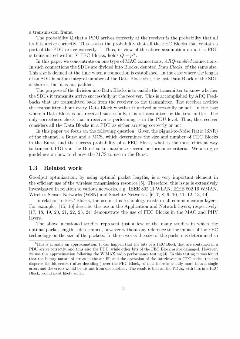
Consider a Burst of L FEC Blocks as shown in Figure 1. We number the FEC Blocksin the Burst from right to left, such that the right most FEC Block is FEC Block 1 and theleft most FEC Block is FEC Block L.In view of the above, we divide the discussion into two cases, F > 2B − 1 and F ≤ 2B − 1.

6

Figure 1: Numbering the FEC Blocks in a Burst

2.2.1 The case F > 2B − 1

Theorem 1. There is an optimal division of the Burst in which the first PDU begins at thebeginning of the left most FEC Block (left edge of the Burst in Figure 1) and every otherPDU either begins immediately after the previous one ( Back-to-Back ) or at the beginningof the next FEC Block following the end of the previous PDU (towards the right edge of theBurst).

Proof. Consider an optimal division of the Burst. If it fulfills the Theorem then we are done.Otherwise, we show how to change the given division so that the new optimal division fulfillsthe Theorem. Notice that if we move a PDU towards the left edge of the Burst, then as longas the beginning of the PDU does not cross a FEC boundary, we either do not change thenumber of FEC Blocks over which the PDU is defined, or we decrement this number by one,increasing the B-Goodput. If the PDU crosses a FEC boundary, then if it returns to the sameexact position within a FEC Block as its original position, then the number of FEC Blocksover which it is defined is not changed. Therefore, if the first PDU is not allocated from theleft edge of a Burst, one can move it to this location without increasing the B-Goodput. Wenow consider the second PDU in the Burst, from the left, and move it an integral number ofF bits until it reaches a point where there is at most one FEC Block boundary between itsstart position and the end of the first PDU. Now, the second PDU can be moved to reachthe end of the first PDU, if it does not cross the boundary of a FEC Block, or otherwiseto the beginning of the FEC Block immediately following the first PDU. By following thisprocess for every PDU, one can generate a division that fulfills the Theorem. �

From now on we consider only divisions that fulfill Theorem 1. We also denote the first(B-1) bits in a FEC Block as the Starting edge of the FEC Block, and the last B bits as theEnding edge.

Theorem 2. In an optimal division of a Burst, every PDU ends either within the Startingedge or within the Ending edge of a FEC Block.

Proof. Consider an optimal division of the Burst. If all the PDUs end within the above edgesof a FEC Block then we are done. Otherwise, let the kth PDU from the left of the Burst,

7

denoted PDUk, to be the first PDU from the left that ends at a bit of a FEC Block which isoutside the above edges. If PDUk+1 begins at the next FEC Block boundary, or in the casethat PDUk is the last PDU in the Burst, one can add at least one Data Block to the Burst,at the end of PDUk, without changing the success probabilities of the existing PDUs, thusincreasing the B-Goodput and contradicting the optimality of the given division.

Therefore, assume that PDUk+1 begins immediately after PDUk. If the success prob-ability of PDUk+1 is larger than that of PDUk then one can move one Data Block fromPDUk to PDUk+1, thus increasing the B-Goodput, contradicting the optimality of the givendivision. If the success probability of PDUk is larger than that of PDUk+1 than again onecan move one Data Block from PDUk+1 to PDUk. The success probability of PDUk is notchanged. The success probability of PDUk+1 can only increase (we shorten PDUk+1), andagain the overall B-Goodput increases, contradicting the optimality of the given division.

It turns out that the success probabilities of PDUk and PDUk+1 must be equal. One cannow move Data Blocks from PDUk to PDUk+1 until one of the following occurs: there areData Blocks left in PDUk but the movement of another Data Block will cause the beginningof PDUk+1 to cross a FEC Block boundary, or there are no Data Blocks left in PDUk. Inthe first case PDUk ends within the Starting edge of a FEC Block. In the second case wecan omit PDUk from the division and move PDUk+1 to begin at either the beginning of aFEC Block or after PDUk−1.

Repeating the above process ends with a division as claimed in the Theory. �

2.3 An algorithm to compute the B-Goodput

Theorems 1 and 2 establish the theoretic basis for a dynamic programming algorithm tofind the optimal division of a Burst. We denote this algorithm by Division-Find. AlgorithmDivision-Find builds a table T of L rows, as the number of FEC Blocks in the Burst. The firstrow of T refers to FEC Block 1 of the Burst and so on. Row number k shows the optimal useof FEC Blocks 1 to k of the Burst, as it is explained in the following. Every row has (2B−1)entries, corresponding to the places within a FEC Block where a PDU can start, followingTheorem 2. These entries of row k are numbered T [k, 1], T [k, 2], ..., T [k, B], T [k, F − (B −2)], ..., T [k, F ].

The entries in T contain an average number of successfully transmitted data bits, andnot Goodputs. The Goodput can be received by dividing the value in an entry by the Burstsize. The entries are computed as follows. In row 1 we fill entries T [1, 1], ..., T [1, B] only.Entry T [1, j], 1 ≤ j ≤ B is computed assuming that a PDU begins at bit number j in theFEC Block and it contains as many Data Blocks as possible. Say for entry T [1, j] one canallocate a PDU of X FEC Blocks, starting from bit number j in the FEC Block. ThenT [1, j] = X ·B · p.

We now move to row k, 2 ≤ k ≤ L − 1. In each of these rows we first compute entriesT [k, F − (B − 2)], ..., T [k, F ] and then entries T [k, 1], ..., T [k, B]. We first handle row 2 andconsider entries T [2, j], F − (B− 2) ≤ j ≤ F . We want to find how the section of the Burst,starting from bit j of the second FEC Block, and ending at the end of the Burst, is mostefficiently used, i.e. how one shall divide this section into PDUs such that the maximal

8

average number of data bits are transmitted successfully. One needs to consider 3 cases,derived from Theorems 1 and 2, as shown in Figure 2, and choose the maximum among the3. Notice that not all the cases always exist. This depends on the relation between O + Bto F , e.g. if O + B is larger than 2B − 1 in Case B then this case actually does not exist.Also notice that in Cases B and C one uses entries from row 1.

Figure 2: Computing entry T [2, j], F − (B − 1) ≤ j ≤ F in the table of algorithm Division-Find

We now move to entries T [2, 1], ..., T [2, B]. Consider entry T [2, j] in this set. We assumethat a PDU begins at bit j of the FEC Block and consider all the possibilities to allocatePDUs at the section of the Burst that begins at bit j of the second FEC Block and thatends at the end of the Burst. We have 3 cases, as shown in Figure 3, again derived fromTheorems 1 and 2. The value of T [2, j] is the maximum among all the cases. Notice that inCase C we use an entry in row 2 that was already computed, and in Case B we use an entryin row 1. Again, it is possible that not all the 3 cases exist.

Concerning row L notice that at most two entries need to be computed. From Theorem 1entry T [L, 1] must be computed. Also, let X ≥ 1 be the largest integer such that O+X ·B ≤F . If X > 0 and O +X · B < F then entry T [L,O +X · B] must also be computed. Thisentry is computed first. Notice that T [L, 1] is the final result of the algorithm.

Lemma 1. The value of every entry in row k of T , 2 ≤ k ≤ L− 1, is computed in O(k)

Proof. Consider an entry T [k, j], F − (B − 2) ≤ j ≤ F . In order to compute this entry oneneeds to consider two possibilities. The first one corresponds to the case that the next PDUbegins at the start of FEC Block number k − 1. This case has the value T [k − 1, 1]. Theother possibility corresponds to the case where a PDU begins at bit j of FEC Block k. This

9

Figure 3: Computing entry T [2, j], 1 ≤ j ≤ B in the table of algorithm Division-Find

PDU can end, according to Theorem 2, at 2(k − 1) different Starting and Ending edges.Thus, we need to choose the maximum among 2(k − 1) + 1 = 2k − 1 cases, where each caseis computed in O(1), possibly using entries from previous rows.

Considering an entry T [k, j], 1 ≤ j ≤ B, the arguments are similar to the case above. �

Theorem 3. The time complexity of Division-Find is O(L2B).

Proof. First consider the computation of the entries in row k, 2 ≤ k ≤ L − 1. In such arow there are 2B − 1 entries and each one is computed in O(k)(Lemma 1). Thus, row k iscomputed in O(B · k). Summing over all the rows k we get that their entries are computedin O(L2B). In row 1 we compute only B entries, each in O(1), and in row L we computeentries T (L, 1) and T [1, O +X · B] (see above) in O(L). The Theorem follows. �

2.3.1 The case F ≤ 2B − 1

Notice that if F ≤ 2B − 1 than a PDU can end at every position within a FEC Block.Therefore, algorithm Division-Find is changed to contain only F entries in any row, and itstime complexity is O(L2F ).

Remark 1. It is sometimes possible to receive the same optimal B-Goodput in a Burst indifferent divisions, such that the divisions contain different number of Data Blocks. Forexample, for L = 2 FEC Blocks, F = 480 bits, B = 45 bits, O = 45 bits and p = 0.9 there

10

are two divisions that yield the maximum B-Goodput. In one division there is one PDU with20 Data Blocks and in another division there are 2 PDUs, each being defined over a separateFEC Block, with 9 Data Blocks each. Our algorithm is implemented to choose the divisionwith the largest number of Data Blocks.

2.4 Modulation/Coding Scheme (MCS) selection

IEEE 802.16e/WiMAX enables the use of the following Modulation/Coding schemes(MCSs) [1]: QPSK-1/2, QPSK-3/4, 16QAM-1/2, 16QAM-3/4, 64QAM-1/2, 64QAM-2/3,64QAM-3/4 and 64QAM-5/6. 64QAM-1/2 is practically not used and so we will not con-sider this scheme any further [45].

Recall that when a Burst is defined, actually it uses slots in the Physical layer. In anyMCS the set of slots in a Burst is divided into groups such that any group is a FEC Block. Inevery MCS it is possible to define groups of slots of different sizes, resulting in FEC Blocks ofdifferent sizes. Here we only consider the largest FEC Blocks that are possible in the MCSs.We denote by j the number of slots, in every MCS, needed to define the largest FEC Block.We show the value of j for every MCS in Table 1, together with F , the number of bits thatthe largest FEC Block contains. We also show the success probability p of the largest FECBlock in every MCS and in several values of the SNR (Signal-to-Noise-Ratio). An entry with∗ stands for N/A, which means that the success probability of a FEC Block in the consideredMCS and SNR is 0 . These probabilities are taken from [50]. The input from [50] containsgraphs that address, for every MCS allowed in WiMAX, and for many realistic SNR values,the success probability for all possible length FEC Blocks in the considered MCS. We seefrom Table 1 that for low SNRs (bad channels) only few MCSs are applicable, while in highSNRs all the MCSs are applicable.

We also see that there is a trade-off in using the set of slots of a Burst. On one handit is possible to decide on a reliable MCS to be used in the Burst. However, the numberof FEC Blocks, and so the number of bits in the Burst, is low. On the other hand, a lessreliable MCS results in more FEC Blocks and bits in the Burst, but with a smaller successprobability of the FEC Blocks.

One criteria to decide on the best MCS is the B-Goodput. In Table 2 we show the B-Goodput for every MCS in every SNR value between 2 to 12 dB, for the case of S = 900 slots,B = 128 bits and O = 104 bits. With O = 104 bits we assume that a PDU contains theGMH and the CRC fields of 6 and 4 bytes respectively as overhead, and one FragmentationSubHeader (FSH) of 3 bytes, which is used when a PDU contains Data Blocks [1]. Accordingto the B-Goodput criteria QPSK-1/2 can be chosen as the best MCS to use in every SNR.However, in QPSK-1/2 the Burst contains only 90 FEC Blocks of 480 bits each. On the otherhand, 64QAM-5/6 contains 450 FEC Blocks of 480 bits each. This enables the transmissionof more bits in the Burst, although with a reduced success probability.

Therefore, in Table 3 we show the average number of Data Blocks that are transmittedsuccessfully in the Burst, again for every MCS in every SNR. According to this criteria, thebest MCS can change from one SNR to another. As the channel becomes better, i.e., higherSNR values, the MCS that enables to transmit a larger number of bits in a Burst is becoming

11

the best MCS to use. For example, in SNR=12 dB the best MCS is 64QAM-5/6 because theB-Goodput of all the MCSs are about the same, but 64QAM-5/6 enables the largest numberof bits in the Burst. For SNR= 9 dB , 64QAM-2/3 enables to transmit successfully thelargest number of Data Blocks, although its B-Goodput is only the 5th in size. The largernumber of bits in a Burst with 64QAM-2/3 enables to compensate for the lower B-Goodput.

3 Maximizing the Data Goodput


We are given an SNR, a Burst of S slots, X Data Blocks of length B bits each and thenumber of PDU overhead bits. The problem that we want to solve is as follows: Given aModulation/Coding Scheme (MCS), how to divide the Burst into PDUs such that the DataGoodput (D-Goodput) is maximized. The given MCS determines the number and the lengthof the FEC Blocks in the Burst, and their success probability.

3.2 Definition of the Data Goodput

We are given:

1. A Burst of L FEC Blocks

2. Every FEC Block contains F bits

3. Every FEC Block has probability p to arrive successfully at the receiver

4. X Data Blocks of length B bits each.

5. Every PDU has O overhead bits. We assume that O < F since according to the IEEE802.16e/WiMAX standard [1] the total length of the overhead fields in a PDU is mostlikely to be smaller than one FEC Block.

We want to transmit the X Data Blocks in the Burst such that the Data Goodput (D-Goodput) is maximized. The D-Goodput is defined as follows: Let D be the number of Databits that are transmitted successfully in the Burst. Then, D-Goodput= D

X·B. D is computed

as follows: Assume that a PDU is defined over k FEC Blocks. Then, the success probabilityof the PDU is pk and every Data Block in the PDU contributes B · pk bits to D. D isthe summation of the contributions of all the Data Blocks. Notice that the D-Goodput iscomputed using X ·B in the denominator, because the Burst is given and we want to use itto transmit to the receiver as many data bits as possible.

Notice also that the maximum number of Data Blocks, Xmax, that can be transmittedin the Burst is

⌊

L·F−OB

⌋

. Thus, if the given X is larger than Xmax it shall be reduced to thisnumber.

12

Following the proof of Theorem 1, one can easily verify that it holds also when lookingfor a division that maximizes the D-Goodput. However, Theorem 2 does not hold. To seethis, consider the following example: We have F = 400 bits, L = 3 FEC Blocks, O = 210bits, X = 4 Data Blocks, B = 145 bits and p = 0.9. There are two optimal divisions in thiscase, in both there are two PDUs. In the first division the first PDU begins at the beginningof the left most FEC Block, and contains 3 Data Blocks. The second PDU begins at thebeginning of the right most FEC Block and it contains one Data Block. In the other divisionthe two PDUs are replaced. The Data Blocks in the longer PDU do not end in the Endingedge of a FEC Block.

Following the above example, we extend the version of algorithm Division Find fromsection 2.3, the version that considers any bit in a FEC Block as a possible starting bit of aPDU. The extension takes into account the finite number of Data Blocks to transmit.

3.3 An algorithm to compute the D-Goodput

We denote the extended algorithm by Limited-Block-Division-Find (LBDF). AlgorithmLBDF builds a 3-D matrix T with the following dimensions: it has L rows, as the num-ber of FEC Blocks in the Burst. The length of every row is F and the depth of the matrixis X , as the number of Data Blocks to transmit. Entry T [r, c, d] refers to the optimal use ofthe section of the Burst, starting from bit c in FEC Block r and using d Data Blocks. Weare looking for T [L, 1, X ].

The first row of T refers to FEC Block 1 of the Burst and so on. Row number k showsthe optimal use of FEC Blocks 1 to k of the Burst, as it is explained in the following. Everyrow has F entries, corresponding to the places within a FEC Block where a PDU can start.

The entries in T contain an average number of successfully transmitted data bits, andnot the D-Goodput. The D-Goodput can be received by dividing the value in an entry by thenumber of Data Blocks in use, multiplied by their size B.

The entries are computed as follows. In row 1 we fill entries T [1, 1, ∗], ..., T [1, F−O−B+1, ∗] only. Entry T [1, j, d], 1 ≤ j ≤ F −O−B+1, 1 ≤ d ≤

⌊

F−j+1−O

B

⌋

is computed assumingthat a PDU begins at bit number j in the FEC Block and it contains d Data Blocks. ThenT [1, j, d] = d ·B · p. Notice that the values of d are limited to the maximum number of DataBlocks that can be allocated in the PDU, from the starting place of the PDU until the endof the FEC Block.

We now move to row k, 2 ≤ k ≤ L − 1. We compute the entries of row k in theorder T [k, F, ∗], T [k, F − 1, ∗], ..., T [k, 1, ∗]. Consider entry T [k, j, d], where d is in the range1, ...,

⌊

k·F−j+1−O

B

⌋

. We want to find how the section of the Burst, starting from bit j of FECBlock k, and ending at the end of the Burst, is most efficiently used by d Data Blocks,i.e. how one shall divide this section into PDUs that contain d Data Blocks such thatthe maximal average number of data bits are transmitted successfully. Entry T [k, j, d] iscomputed as follows. First, we consider the possibility that all the d Data Blocks will beallocated starting from the beginning of FEC Block k − 1. Then, we assume that a PDUbegins at bit j, denoted PDU ′, and first assume that PDU ′ contains one Data Block andthe rest of the Burst contains d − 1 Data Blocks. Then we assume that PDU ′ contains 2

13

Data Blocks and assume that the rest of the Burst contains d − 2 Data Blocks and so onuntil PDU ′ contains d Data Blocks. See Figure 4. The value of T [k, j, d] is the maximumamong the d+ 1 possibilities.

Figure 4: Computing entry T [k, j, d] in Algorithm LBDF

Concerning row L notice that only entries T [L, 1, ∗], T [L,O + B + 1, ∗], T [L,O + 2B +1, ∗], ..., T [L,O + X ′ · B + 1, ∗] need to be computed, where X ′ =

⌊

F−OB

⌋

and X ′ > 0. IfX ′ = 0 only entry T[L,1,*] need to be computed.

Lemma 2. Entry T [k, j, d] 2 ≤ k ≤ L is computed in O(d)

Proof. For entry T [k, j.d] we consider at most d+1 possibilities. Each possibility is computedin O(1) since it involves a direct computation and a look in an entry of the matrix that wasalready computed. �

Theorem 4. The time complexity of LBDF is O(L · F ·X2).

Proof. There are L rows in T . In every row one computes at most F ·X entries. By Lemma 2every entry is computed in O(X). The Theorem follows. �

14

3.4 Determining the Modulation/Coding scheme in the Burst

Using the same reasoning as in Section 2.4 , a question now arises: Given a number X ofData Blocks, of size B bits each, and a Burst of S slots, what is the best MCS to use in theBurst such that the D-Goodput is maximized. In the following we show the mutual influencebetween the number of FEC Blocks in a Burst, and their size, and the Data Blocks’ sizes B,on the resulting D-Goodput.

We begin with B = 128 bits. In Figure 5(A) we assume an SNR of 3.5 dB where onlyQPSK-1/2, QPSK-3/4 and 16QAM-1/2 are applicable ( see Table 1), with p = 0.999, 0.998and 0.82 respectively. We also assume that O = 104 bits, X = 6 Data Blocks and 4 Bursts’sizes of 30, 60, 90 and 120 slots. In this case, since X is relatively small, every FEC Blockcan be a separate PDU in each of the three MCSs. Therefore, the D-Goodput in each of theMCSs equals to p. QPSK-1/2 has the largest p in this SNR, 0.999, and therefore it has thelargest D-Goodput.

Consider Figure 5(B) now. In this case we assume an SNR of 4.5 dB, O = 104 bits andX = 10 Data Blocks. Again, only QPSK-1/2, QPSK-3/4 and 16QAM-1/2 are applicable inthis SNR, with p equals to 0.999, 0.999 and 0.998 respectively. In QPSK-1/2 and a Burst sizeof 30 slots, there are 3 FEC Blocks. One must define only one PDU over the 3 FEC Blocksin order to be able to transmit all the X = 10 Data Blocks. The PDU success probabilityand the D-Goodput are therefore 0.9993 = 0.997. However, in QPSK-3/4 and 16QAM-1/2,which enable more FEC Blocks in the Burst, it is possible to define every FEC Block to bea separate PDU. In this case QPSK-3/4 results with the best D-Goodput of 0.999 . For theother Burst sizes it is also possible in QPSK-1/2 to define every FEC Block to be a separatePDU. Therefore, QPSK-1/2, together with QPSK-3/4, has the largest D-Goodput of 0.999 .

In Figure 5(C) we show results for SNR of 4.5 dB, O = 104 bits and X = 16 DataBlocks. In QPSK-1/2 and a Burst size of 30 slots, it is possible to transmit at most 10Data Blocks. Therefore, QPSK-1/2 is not applicable in this Burst size. In QPSK-3/4 thereare 5 FEC Blocks in a Burst of 30 slots and one can transmit the X = 16 Data Blocksonly if one PDU is defined over the 5 FEC Blocks. Therefore, the PDU success probabilityand the D-Goodput are 0.9995 = 0.995. In 16QAM-1/2 there are 6 FEC Blocks and theoptimal division of the Burst is into 8 PDUs. 4 PDUs are defined over one FEC Block andeach contains 2 Data Blocks. Additional 2 PDUs are defined over 2 FEC Blocks and eachcontains 2 Data Blocks. One additional PDU is defined over 2 FEC Blocks and it contains 3Data Blocks. The last PDU is defined over 2 FEC Blocks and it contains one Data Block. Itturns out that 16QAM-1/2 has the largest D-Goodput, 0.997 , although it has the smallestp. For the Burst size of 60 slots it is possible in QPSK-3/4 and 16QAM-1/2 to define everyFEC Block to be a separate PDU, and therefore the D-Goodput is p. QPSK-3/4 has a largerp than 16QAM-1/2, 0.999 vs. 0.998, and therefore it has a larger D-Goodput. In QPSK-1/2the optimal division of the Burst is into 8 PDUs. Four PDUs are defined over one FECBlock and each contains 2 Data Blocks, 2 PDUs are defined over 2 FEC Blocks and eachcontains 3 Data Blocks. Another 2 PDUs are defined over 2 FEC Blocks and each containsone Data Block. Therefore, the D-Goodput of QPSK-1/2 is 0.998 . For the Burst sizes of90 and 120 slots it is also possible in QPSK-1/2 to define every FEC Block to be a separate

15

PDU. Therefore, QPSK-1/2, together with QPSK-3/4, has the largest D-Goodput.We now turn to B = 512 bits. With this size of the Data Blocks and a PDU overhead

of O = 104 bits, 2 FEC Blocks are needed to contain one Data Block in all the MCSs. Seethe size of F in Table 1. However, with 3 FEC Blocks it is possible to define 2 PDUs overthem, each PDU contains one Data Block and being defined over 2 FEC Blocks.

In Figure 5(D) we show results for SNR of 3.5 dB, O = 104 bits and X = 1 Data Block.In this case, since X is relatively small, every 2 FEC Blocks are a PDU in each of the 3MCSs. QPSK-1/2 has the largest p in this SNR, 0.999, and therefore it yields the largestD-Goodput, 0.9992 = 0.998.

In Figure 5(E) we show results for SNR of 4.5 dB, O = 104 bits and X = 3 Data Blocks.In QPSK-1/2 and a Burst size of 30 slots, it is possible to transmit at most 2 Data Blocks.Therefore, QPSK-1/2 is mot applicable for this Burst size. In QPSK-3/4 it is possible totransmit the X = 3 Data Blocks in 3 PDUs of 2 FEC Block each, with a PDU successprobability and D-Goodput of 0.9992 = 0.998. In 16QAM-1/2 it is also optimal to transmitthe Data Blocks in PDUs of 2 FEC Blocks. Since p is larger in QPSK-3/4, it has a largerD-Goodput. For the other Burst sizes it is possible in all the considered MCSs to definePDUs of 2 FEC Blocks. Since QPSK-1/2 and QPSK-3/4 have the largest p of 0.999, theseMCSs also have the largest D-Goodput.

In Figure 5(F) we show results for SNR of 3.5 dB, O = 104 bits and X = 4 Data Blocks.Again, QPSK-1/2 is not applicable in the Burst size of 30 slots. With 16QAM-1/2 onecan transmit the X = 4 Data Blocks in 4 PDUs, each defined over 2 FEC Blocks. WithQPSK-3/4 one can transmit the X = 4 Data Blocks only if one PDU is defined over 6 FECBlocks. However, since QPSK-3/4 has a much larger p than 16QAM-1/2, it still has a largerD-Goodput than 16QAM-1/2, p6 = 0.994 in QPSK-3/4 vs. p2 = 0.672 in 16QAM-1/2. Forthe Burst sizes of 60, 90 and 120 slots it is possible in all the considered MCSs to definePDUs over 2 FEC Blocks. Therefore, QPSK-1/2 and QPSK-3/4, which have the largest p,also have the largest D-Goodput of 0.9992 = 0.998 and 0.9982 = 0.996 respectively.

We now turn to B = 1024 bits. With this size of the Data Blocks and a PDU overhead ofO = 104 bits, at least 3 FEC Blocks are needed to contain one Data Block in all the MCSs.See the size of F in Table 1. However, with 5 FEC Blocks it is possible to define 1 PDUwhich contains 2 Data Blocks.

In Figure 5(G) we show results for SNR of 3.5 dB, O = 104 bits and X = 1 Data Block.In this case one must define one PDU of 3 FEC Blocks in each of the 3 MCSs. QPSK-1/2has the largest p in this SNR, 0.999, and therefore it also has the largest D-Goodput of0.9993 = 0.997.

In Figure 5(H) we show results for SNR of 4.5 dB, O = 104 bits and X = 2 DataBlocks. QPSK-1/2 is not applicable in the Burst size of 30 slots. In QPSK-3/4 one musttransmit the X = 2 Data Blocks in one PDU of 5 FEC Blocks and therefore the D-Goodputis 0.9995 = 0.995. In 16QAM-1/2 one can transmit the X = 2 Data Blocks in 2 separatePDUs, each defined over 3 FEC Blocks, therefore the D-Goodput is 0.9983 = 0.994. SinceQPSK-3/4 has a larger p, it still has a larger D-Goodput than 16QAM=1/2. For the otherBurst sizes it is possible in all the 3 MCSs to transmit every Data Block in a separate PDU

16

of 3 FEC Blocks. Since QPSK-1/2 and QPSK-3/4 have the largest p of 0.999, they also havethe largest D-Goodput.

The outcome from all the above examples is that sometimes it is more efficient to use lessreliable MCSs. There are two reasons for this outcome: First, less reliable MCSs sometimesenable the transmission of all the X Data Blocks while more reliable MCSs do not enable thistransmission. Second, the large number of bits in the less reliable MCSs enables to definesmaller PDUs, with a larger success probability than the PDUs in more reliable MCSs. Thiscompensates for the smaller success probability of a single FEC Block in the former MCSs.

We further elaborate on these reasons in Figures 6 and 7. In Figure 6 we assume six Burstsizes of 30, 60, 90, 120, 150 and 180 slots. We also assume the following MCSs: QPSK-1/2,QPSK-3/4 and 16QAM-1/2. For every MCS and Burst size we show the maximum numberof Data Blocks that can be transmitted in the Burst. We assume B = 128, 512 and 1024 inFigures 6(A), (B) and (C) respectively. We see that the smallest number of Data Blocks isreceived in QPSK-1/2, while the largest one is received in 16QAM-1/2. The reason is thatin both QPSK-1/2 and 16QAM-1/2 holds that F = 480 bits. However, in QPSK-1/2 holdsj = 10 while in 16QAM-1/2 holds j = 5. Thus, in 16QAM-1/2 there is twice the number ofFEC Blocks than in QPSK-1/2.

Notice that the graphs are not linear. This is because the Bursts are not always utilizedcompletely. For example, in Figure 6(C) we show the case for B = 1024. In QPSK-1/2and a Burst size of 120 slots the maximum number of Data Blocks is 5 and there are 536bits that are unused. These 536 unused bits are computed as follows : there are 5760 bitsin the Burst (12 · 480). 104 bits are used for a PDU overhead. In the rest of the bits oneinserts as many Data Blocks as possible, which is 5. Therefore, the number of unused bitsis 5760 − 104 − 5 · 1024 = 536. In a Burst size of 150 slots the maximum number of DataBlocks is 6 with 952 unused bits, and in a Burst size of 180 slots the maximum number ofData Blocks is 8 with 344 unused bits. One can see that when the Burst size grows from 120to 150 slots the number of unused bits increases and the number of Data Blocks increases by1. However, when the Burst size grows from 150 to 180 slots the relatively larger number ofunused bits in the Burst size of 150 slots allows to increase the number of Data Blocks by 2.

Consider Figure 7 now. We assume the same six Burst sizes and the same set of MCSsas in Figure 6. We assume an SNR of 4.5 dB and therefore, from Table 1, recall that thesuccess probabilities of the FEC Blocks are 0.999, 0.999 and 0.998 in QPSK-1/2, QPSK-3/4and 16QAM-1/2 respectively. In Figure 7(A) we assume that the number X of Data Blocksis the maximum that can be transmitted in QPSK-1/2 where B = 128 bits. For example,for a Burst size of 30 slots, X = 10, for a Burst size of 60 slots X = 21 etc. We denote thisscenario by ’QPSK-1/2 saturated”. In this scenario, when using QPSK-1/2, it is required totransmit all the X Data Blocks in one or two PDUs ( the case of 2 PDUs is when the numberof unused bits is larger than the PDU overhead but it is smaller than a Data Block size ). InQPSK-3/4 PDUs are of 1 or 2 FEC Blocks only, and in 16QAM-1/2 it is possible to transmitall the Data Blocks in PDUs of one FEC Block. Therefore, in QPSK-3/4 and 16QAM-1/2the PDU success probability is p (or sometimes p2 for the most) while for QPSK-1/2, whenone PDU is used, it is pL where L is the number of FEC Blocks in the Burst. As the

17

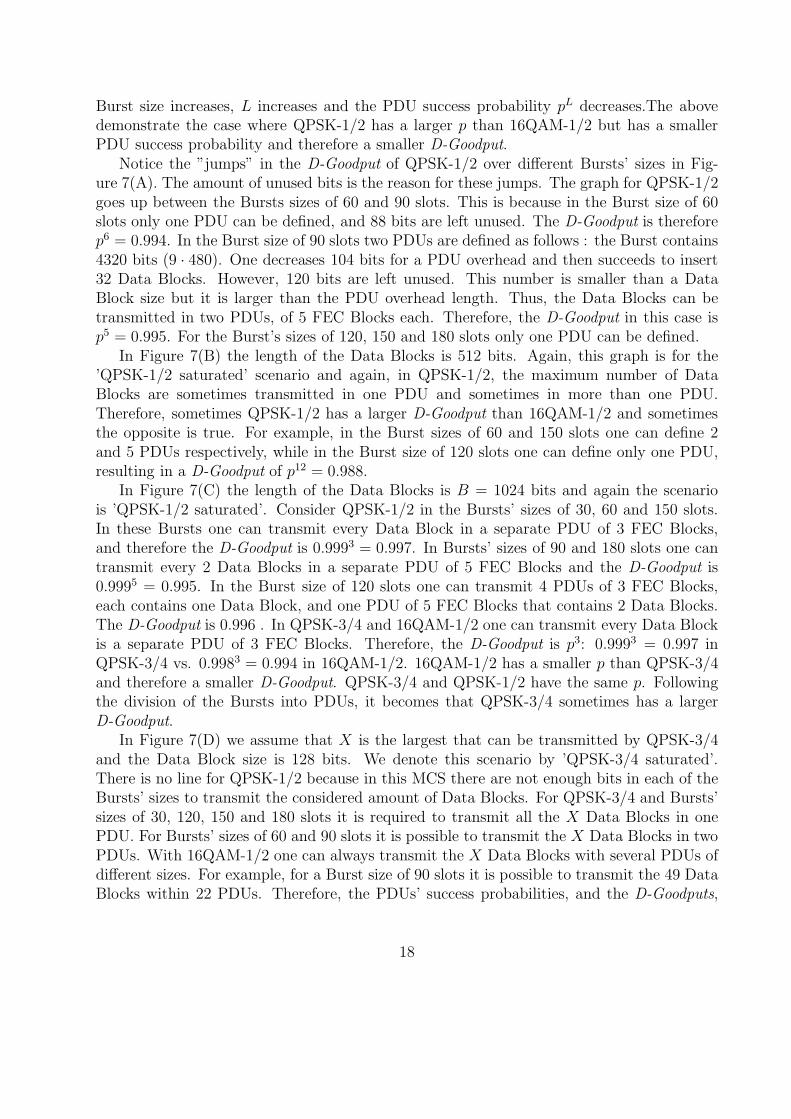
Burst size increases, L increases and the PDU success probability pL decreases.The abovedemonstrate the case where QPSK-1/2 has a larger p than 16QAM-1/2 but has a smallerPDU success probability and therefore a smaller D-Goodput.

Notice the ”jumps” in the D-Goodput of QPSK-1/2 over different Bursts’ sizes in Fig-ure 7(A). The amount of unused bits is the reason for these jumps. The graph for QPSK-1/2goes up between the Bursts sizes of 60 and 90 slots. This is because in the Burst size of 60slots only one PDU can be defined, and 88 bits are left unused. The D-Goodput is thereforep6 = 0.994. In the Burst size of 90 slots two PDUs are defined as follows : the Burst contains4320 bits (9 · 480). One decreases 104 bits for a PDU overhead and then succeeds to insert32 Data Blocks. However, 120 bits are left unused. This number is smaller than a DataBlock size but it is larger than the PDU overhead length. Thus, the Data Blocks can betransmitted in two PDUs, of 5 FEC Blocks each. Therefore, the D-Goodput in this case isp5 = 0.995. For the Burst’s sizes of 120, 150 and 180 slots only one PDU can be defined.

In Figure 7(B) the length of the Data Blocks is 512 bits. Again, this graph is for the’QPSK-1/2 saturated’ scenario and again, in QPSK-1/2, the maximum number of DataBlocks are sometimes transmitted in one PDU and sometimes in more than one PDU.Therefore, sometimes QPSK-1/2 has a larger D-Goodput than 16QAM-1/2 and sometimesthe opposite is true. For example, in the Burst sizes of 60 and 150 slots one can define 2and 5 PDUs respectively, while in the Burst size of 120 slots one can define only one PDU,resulting in a D-Goodput of p12 = 0.988.

In Figure 7(C) the length of the Data Blocks is B = 1024 bits and again the scenariois ’QPSK-1/2 saturated’. Consider QPSK-1/2 in the Bursts’ sizes of 30, 60 and 150 slots.In these Bursts one can transmit every Data Block in a separate PDU of 3 FEC Blocks,and therefore the D-Goodput is 0.9993 = 0.997. In Bursts’ sizes of 90 and 180 slots one cantransmit every 2 Data Blocks in a separate PDU of 5 FEC Blocks and the D-Goodput is0.9995 = 0.995. In the Burst size of 120 slots one can transmit 4 PDUs of 3 FEC Blocks,each contains one Data Block, and one PDU of 5 FEC Blocks that contains 2 Data Blocks.The D-Goodput is 0.996 . In QPSK-3/4 and 16QAM-1/2 one can transmit every Data Blockis a separate PDU of 3 FEC Blocks. Therefore, the D-Goodput is p3: 0.9993 = 0.997 inQPSK-3/4 vs. 0.9983 = 0.994 in 16QAM-1/2. 16QAM-1/2 has a smaller p than QPSK-3/4and therefore a smaller D-Goodput. QPSK-3/4 and QPSK-1/2 have the same p. Followingthe division of the Bursts into PDUs, it becomes that QPSK-3/4 sometimes has a largerD-Goodput.

In Figure 7(D) we assume that X is the largest that can be transmitted by QPSK-3/4and the Data Block size is 128 bits. We denote this scenario by ’QPSK-3/4 saturated’.There is no line for QPSK-1/2 because in this MCS there are not enough bits in each of theBursts’ sizes to transmit the considered amount of Data Blocks. For QPSK-3/4 and Bursts’sizes of 30, 120, 150 and 180 slots it is required to transmit all the X Data Blocks in onePDU. For Bursts’ sizes of 60 and 90 slots it is possible to transmit the X Data Blocks in twoPDUs. With 16QAM-1/2 one can always transmit the X Data Blocks with several PDUs ofdifferent sizes. For example, for a Burst size of 90 slots it is possible to transmit the 49 DataBlocks within 22 PDUs. Therefore, the PDUs’ success probabilities, and the D-Goodputs,

18

are larger in 16QAM-1/2 than in QPSK-3/4 .In Figure 7(E) we assume again the ’QPSK-3/4 saturated’ scenario, with Data Blocks

of 512 bits. In QPSK-3/4 and Burst’s size between 30 to 150 slots, one can transmit the XData Blocks within several PDUs. However, every PDU is defined over more than 2 FECBlocks. In the Burst size of 180 slots only one PDU can be used. In 16QAM-1/2 every DataBlock is transmitted in a separate PDU of 2 FEC Blocks and therefore 16QAM-1/2 has alarger D-Goodput than QPSK-3/4 in all the Burst’s sizes.

In Figure 7(F) we assume the ’QPSK-3/4 saturated’ scenario with Data Blocks of 1024bits. In 16QAM-1/2 every Data Block is transmitted in a separate PDU of 2 FEC Blocksand so the D-Goodput is 0.9983 = 0.994. In QPSK-3/4 every 2 Data Blocks are transmittedin a separate PDU of 5 FEC Blocks, and so the D-Goodput is 0.9995 = 0.995.

19

4 The optimal Burst size for data transmission


In this section we are given an SNR (dB), a number X of Data Blocks to transmit and thenumber of the PDU’s overhead bits. We are looking for the optimal Burst size to transmitthese Data Blockst according to 3 possible performance criteria. For each criteria we alsodecide on the best MCS to use in the given SNR.

The first performance criteria is Max-Bits which maximizes the number of successfullytransmitted data bits in the Burst. The second criteria is Burst-Goodput (B-Goodput) thatmaximizes the ratio between the number of successfully transmitted data bits in the Burst,to the Burst size. The third criteria, Slot-Goodput (S-Goodput), maximizes the number ofsuccessfully transmitted data bits per transmission slot.When we consider a MCS in the given SNR, we are actually being given a FEC Block’s sizeF and a FEC Block’s success probability p. This probability is determined by the givenSNR ( see Table 1 ). Thus, for every MCS the input we have is:

1. X Data Blocks to transmit in a Burst.

2. FEC Blocks that contain F bits each.

3. Every FEC Block has probability p to arrive successfully at the receiver.

4. Every PDU has O overhead bits, O < F from the same reasons as in Section 2.

For each of the performance criteria we look for the Burst size that maximizes the criteriain the considered MCS. Then, the MCS in which the best result is achieved, is the one touse in the given SNR.

In sections 4.2, 4.3 and 4.4 we deal with the Max-Bits, Burst-Goodput and with theSlot-Goodput criteria respectively. In section 4.5 we compare among the three.

4.2 The Max-Bits criteria

In this section we are given X Data Blocks to transmit in a Burst and we look for the Burstsize that maximizes the Max-bits criteria. Let O be the number of PDU overhead bits andB the Data Block size. Also assume that (t − 1) · F < O + B ≤ t · F , for some t integer,t ≥ 1. Then, the largest possible value for Max-bits is X · B · pt, where p is the FEC Blocksuccess probability, and we look for the minimal size Burst that enables this Max-Bits value.The following discussion is divided according to the following possible values of t : t = 1,t = 2, t ≥ 3.

4.2.1 Case 1: t = 1, O +B ≤ F

In this case the maximum Max-Bits value is X · B · p. This means that every PDU mustbe allocated over one FEC Block only. Let Y =

⌊

F−OB

⌋

be the maximum number of DataBlocks that can be transmitted within one PDU in one FEC Block.

20

Theorem 5. Given X Data Blocks one needs⌈

XY

⌉

FEC Blocks at minimum to be able totransmit all the X Data Blocks such that the Max-Bits value is X · B · p.

Proof. In order to keep p as the PDU success probability, a PDU can not cross the boundaryof a FEC Block. Therefore, every PDU is defined within one FEC Block and a FEC Block cancontain at most Y Data Blocks. Therefore, one needs

⌈

XY

⌉

FEC Blocks for the transmissionof the X Data Blocks. �

4.2.2 Case 2: t = 2, F < O +B ≤ 2F

In this case the maximum value for Max-bits is X · B · p2 and so a PDU can be definedover two FEC Blocks only. In the following we use several definitions, based on Figure 8.In Figure 8 there are 3 PDUs. PDUs 1 and 2 are allocated starting at the beginning of aFEC Block. We denote such PDUs PDUs that are allocated from the beginning of a FECBlock. PDU 3 is allocated immediately (B2B) after PDU 2. We say that PDUs 2 and 3 areallocated Back-to-Back (B2B). PDU 1 is a stand alone PDU because no PDU is allocatedimmediately after it.

Notice now that in any allocation of PDUs over a Burst such that every PDU is allocatedover 2 FEC Blocks only, there can be stand alone PDUs and groups of PDUs that areallocated B2B.

Let Y =⌊

2F−OB

⌋

be the maximum number of Data Blocks that can be allocated in aPFU over two FEC Blocks.

We now prove several lemmas concerning the allocation of PDUs such that every PDUis allocated over 2 FEC Blocks only. We will use the terms:

• Allocation with p2: An allocation of PDUs in a Burst such that all the PDUs in theBurst have a success probability of p2.

• PDU arrangement with p2: This is an Allocation with p2 such that every stand alonePDU and the first PDU (say from the left) of every group of B2B PDUs are allocatedfrom the beginning of a FEC Block.

Lemma 3. Assume X Data Blocks that are allocated in a Burst of L FEC Blocks with p2.Then, these X Data Blocks can be allocted in the L FEC Blocks in a PDU arrangement withp2.

Proof. In the proof of Theorem 1 it is explained that moving a PDU towards the left side ofa Burst until reaching at a starting edge of a FEC Block or at the end of the previous PDU,which ever comes first, does not change the number of FEC Blocks over which the PDU isallocated.

Therefore, consider the given allocation of the X Data Blocks, and consider the PDUsfrom left to right. We now move the left most PDU to the first starting edge of a FEC Blockon its left. The second PDU is moved in the manner described above and so on. The processis done in the L FEC Blocks and ends with a PDU arrangement with p2 �

21

Lemma 4. Consider a PDU arrangement with p2 of one B2B group of PDUs such that: thegroup is allocated in L FEC Blocks, the group of PDUs contains X Data Blocks and the firstPDU in the group contains less than Y Data Blocks. Then, the above X Data Blocks can beallocated in a PDU arrangement with p2 in the L FEC Blocks such that the first PDU in thefirst group of PDUs contains X Data Blocks if X < Y , and Y Data Blocks otherwise.

Proof. If X < Y then all the Data Blocks can be allocated in one PDU. Otherwise, onebegins to move Data Blocks from the second PDU (from the left) to the first one, until thereare Y Data Blocks in the first PDU, or there are no Data Blocks left in the second PDU.This process continues until there are Y Data Blocks in the first PDU. The above processis carried out within the L FEC Blocks, with p2. The PDU arrangement with p2 is nowreceived by Lemma 3. �

Lemma 5. Consider two PDUs, PDU 1 and PDU 2, that are allocated B2B such that PDU1 is allocated at the beginning of a FEC Block and it contains Y Data Blocks. Then, PDU2 can contain only one Data Block.

Proof. Notice that O + Y · B > 2F − B and O + B > F . Combining the two inequalitiestogether we receive that 2O+Y ·B+2B > 3F . Therefore, if PDU 1 contains Y Data Blocksthen PDU 2 can contain at most one Data Block. �

Lemma 6. Assume PDUs 1,...,k are allocated B2B such that PDU 1 is allocated at thebeginning of a FEC Block and it contains Y Data Blocks. Then PDUs 2,...,k contain oneData Block each.

Proof. In lemma 5 we prove that PDU 2 contains only one Data Block. By the same line ofproof as in Lemma 3 one can now show that PDU 3 contains one Data Block and so on. �

Corollary 6. Follwing Lemmas 3- 6 one can assume that every Burst in which PDUs areallocated such that the success probability of every PDU is p2 is a PDU arrangenet with p2

such that every group of B2B PDUs either contains one PDU with at most Y Data Blocks,or it contains more than one PDU such that the first PDU contains Y Data Blocks and theother PDUs contain one Data Block each.

We now describe algorithm p2-allocation that allocates X Data Blocks in a minimalnumber of FEC Blocks with p2.

Algorithm p2-allocation

Input:X: number of Data BlocksB: size of a Data Block (bits)F: size of a FEC Block (bits)O: size of a PDU overhead (bits)

O < F, F < O +B ≤ 2F

22

Output: L, the minimal number of FEC Blocks in which the X Data Blocks are allocatedwith p2, and the allocation

Compute:1. Y =

⌊

2F−OB

⌋

;X = Z · Y +R, 0 ≤ R ≤ Y − 1.2. if (Y > 1)2.1 Allocate Z PDUs with Y Data Blocks each.2.2 Each PDU is defined over 2 FEC Blocks, starting at the beginning of a FEC Block.2.3 if (R = 0)2.3.1. L = 2 · Z; exit2.4 else if (R ≥ 2)2.4.1 Allocate a new PDU with R Data Block over 2 FEC Blocks.2.4.2 L = 2 · Z + 2; exit2.5 else if (R = 1)2.5.1 ∆ = 2F − (O + Y ·B)2.5.2 if ((∆ + F ≥ O +B) and (Z>0))2.5.2.1 Allocate a new PDU of one Data Block B2B to the last PDU of Y Data Blocks;2.5.2.2 L = 2 · Z + 1; exit2.5.3 else2.5.3.1 Allocate a new PDU with one Data Block over 2 FEC Blocks2.5.3.2 L = 2 · Z + 2; exit3. else (Y = 1;R = 0)3.1 Let N be the maximum number of PDUs that can be defined B2B3.2 Compute X = w ·N + c; 0 ≤ c ≤ N − 13.3 Allocate w groups of N B2B PDUs3.4 Allocate a group of c B2B PDUs3.5 if (c > 0) L = w · (N + 1) + (c+ 1) else L = w · (N + 1); exit

Correctness proof for Algorithm p2-allocation

Theorem 7. Algorithm p2-allocation allocates the X Data Blocks with p2 in the minimalnumber of FEC Blocks.

We prove the correctness of Algorithm p2-allocation for all the possible cases that arespecified in the algorithm. For the proof we need another definition, also based on Figure 8.In this figure notice that PDU 1 crosses the starting edge of FEC 3. We say that a PDUcrosses over the edge of a FEC Block S when it is defined over FEC Blocks S and S + 1.Notice that every PDU that is defined over 2 FEC Blocks crosses the starting edge of exactlyone FEC Block.

We now specify the 5 cases that Algorithm p2-allocation handles and prove the correctnessof each case in Lemmas 7- 11 respectively.

Case 1: Y > 1, R = 0, lines 2.2, 2.3, 2.3.1 . In this case (2 · Z) FEC Blocks are used. Every2 FEC Blocks contain one PDU of Y Data Blocks.

23

Case 2: Y > 1, R ≥ 2, lines 2.2, 2.4, 2.4.1, 2.4.2 . In this case (2 · Z + 2) FEC Blocks areused. Every 2 FEC Blocks contain one PDU of Y Data Blocks, except the last PDU thatcontains R Data Blocks.Case 3: Y > 1, R = 1, lines 2.2, 2.5-2.5.2.2 . In this case (2 · Z + 1) FEC Blocks are used.Every 2 FEC Blocks contain one PDU of Y Data Blocks, except the last one that containsone Data Block, and the last PDU is allocated B2B to the last PDU that contains Y DataBlocks.Case 4: Y > 1, R = 1, lines 2.2, 2.5.3-2.5.3.2 . In this case (2 · Z + 2) FEC Blocks are used.Every 2 FEC Blocks contain one PDU of Y Data Blocks, except the last one that containsone Data Block.Case 5: Y = 1, R = 0, lines 3 - 3.5 . We assume that c > 0. The case of c = 0 is handled bythe same way. In case c > 0 holds that w · (N + 1) + (c+ 1) FEC Blocks are used. N is themaximum number of PDUs that can be allocated B2B. w = XmodN and c = X − w · N .In this case every PDU contains one Data Block. There are w groups of N B2B PDUs andone group of c B2B PDUs.

Notice that the success probabilities of all the PDUs in all the cases is p2. We just needto show that this is achieved in the minimal number of FEC Blocks.

Lemma 7. In case 1 the minimal number of FEC Blocks that is needed to enable the allo-cation of X Data Blocks with p2 is 2 · Z.

Proof. Notice that Algorithm p2-allocation uses 2 · Z FEC Blocks and Z PDUs. It is notpossible to use a lower number of PDUs because then there will be at least one PDU withmore than Y Data Blocks and such a PDU will be allocated over more than 2 FEC Blocks,with a success probability that is lower than p2. Therefore, assume that one can use only2 · Z − 1 FEC Blocks with Z + t PDUs, t ≥ 0, and with p2. Notice that in a Burst of2 · Z − 1 FEC Blocks there are 2 · Z − 1 starting edges of FEC Blocks, and Z + t of themare crossed by PDUs. Therefore, PDUs can start only at (2 · Z − 1)− (Z + t) = Z − t− 1starting edges of FEC Blocks. Therefore, in the Z + t PDUs one can allocate at most(Z − t− 1)Y + 2t+1 Data Blocks (Corollary 6). However, one needs to allocate Z · Y DataBlocks and Z · Y − [(Z − t − 1)Y + 2t + 1] = Y (t + 1) − 2t − 1 > 0 for Y ≥ 2. Therefore,2 · Z − 1 FEC Blocks are not sufficient. �

Lemma 8. In case 2 the minimal number of FEC Blocks that is needed to enable the allo-cation of X Data Blocks with p2 is 2 · Z + 2.

Proof. Notice that Algorithm p2-allocation uses 2 ·Z +2 FEC Blocks and Z +1 PDUs. It isnot possible to use a lower number of PDUs because then there will be at least one PDU withmore than Y Data Blocks and such a PDU will be allocated over more than 2 FEC Blocks,with a success probability that is lower than p2. Therefore, assume that one can use only2 ·Z+1 FEC Blocks with Z+ t PDUs, t ≥ 1, and with p2. Notice that in a Burst of 2 ·Z+1FEC Blocks there are 2 ·Z + 1 starting edges of FEC Blocks, and Z + t of them are crossedby PDUs. Therefore, PDUs can start only at (2 ·Z +1)− (Z + t) = Z − t+1 starting edgesof FEC Blocks. Therefore, in the Z + t PDUs one can allocate at most (Z − t+1)Y +2t− 1

24

Data Blocks (Corollary 6). However, one needs to allocate Z · Y + R Data Blocks andZ · Y + R − [(Z − t + 1)Y + 2t − 1] = Y (t − 1) + R − 2t + 1 > 0 for Y ≥ 2 and R ≥ 2.Therefore, 2 · Z + 1 FEC Blocks are not sufficient. �

Lemma 9. In case 3 the minimal number of FEC Blocks that is needed to enable the allo-cation of X Data Blocks with p2 is 2 · Z + 1.

Proof. Notice that Algorithm p2-allocation uses 2 · Z + 1 FEC Blocks and Z + 1 PDUs. Itis not possible to use a lower number of PDUs because then there will be at least one PDUwith more than Y Data Blocks and such a PDU will be allocated over more than 2 FECBlocks, with a success probability that is lower than p2. Therefore, assume that one canuse only 2 · Z FEC Blocks with Z + t PDUs, t ≥ 1, and with p2. Notice that in a Burstof 2 · Z FEC Blocks there are 2 · Z starting edges of FEC Blocks, and Z + t of them arecrossed by PDUs. Therefore, PDUs can start only at 2 · Z − (Z + t) = Z − t starting edgesof FEC Blocks. Therefore, in the Z + t PDUs one can allocate at most (Z − t) · Y + 2tData Blocks (Corollary 6). However, one needs to allocate Z · Y + 1 Data Blocks andZ · Y + 1− [(Z − t)Y + 2t] = Y · t− 2t+ 1 > 0 for Y ≥ 2. Therefore, 2 · Z FEC Blocks arenot sufficient. �

Lemma 10. In case 4 the minimal number of FEC Blocks that is needed to enable theallocation of X Data Blocks with p2 is 2 · Z + 2.

Proof. Notice that Algorithm p2-allocation uses 2 · Z + 2 FEC Blocks and Z + 1 PDUs. Itis not possible to use a lower number of PDUs because then there will be at least one PDUwith more than Y Data Blocks and such a PDU will be allocated over more than 2 FECBlocks, with a success probability that is lower than p2. Therefore, assume that one can useonly 2 · Z + 1 FEC Blocks with Z + t PDUs, t ≥ 1, and with p2.

Notice that Case 4 is performed since the condition in line 2.5.2 does not hold. I.e. it isnot possible to allocate a PDU with one Data Block B2B after a PDU of Y Data Blocks. Inview of Corollary 6 this means that it is not possible to define B2B PDUs !

Notice that in a Burst of 2 · Z + 1 FEC Blocks there are 2 · Z + 1 starting edges ofFEC Blocks, and Z + t of them are crossed by PDUs. Therefore, PDUs can start onlyat (2 · Z + 1) − (Z + t) = Z − t + 1 starting edges of FEC Blocks. Therefore, in theZ + t PDUs one can allocate at most (Z − t + 1)Y Data Blocks (Corollary 6 and recallthat there are not B2B PDUs). However, one needs to allocate Z · Y + 1 Data Blocks andZ · Y + 1 − [(Z − t + 1)Y ] = Y (t− 1) + 1 > 0 for Y ≥ 2. Therefore, 2 · Z + 1 FEC Blocksare not sufficient. �

Lemma 11. In case 5 and c > 0 the minimal number of FEC Blocks that is needed to enablethe allocation of X Data Blocks with p2 is w · (N + 1) + (c+ 1). N is the maximum numberof PDUs that can be allocated B2B. w = XmodN and c = X − w · N . (The case c = 0 ishandled by the same way ).

Proof. Notice that Algorithm p2-allocation uses w·(N+1)+(c+1) FEC Blocks and w·N+c =X PDUs. It is not possible to use a lower number of PDUs because then there will be at least

25

one PDU with more than one Data Block and such a PDU will be allocated over more than2 FEC Blocks, with a success probability that is lower than p2. It is also not possible to usemore PDUs than w ·N + c ( because otherwise there will be more PDUs than Data Blocks). Therefore, assume that one can use only w · (N +1)+ c FEC Blocks with w ·N + c PDUsand with p2. Notice that in a Burst of w · (N + 1) + c FEC Blocks there are w · (N + 1) + cstarting edges of FEC Block, and w ·N + c of them are crossed by PDUs. Therefore, PDUscan start only at w · (N + 1) + c− [w ·N + c] = w starting edges of FEC Blocks. Therefore,in the Burst one can allocate at most w · N Data Blocks. However, one needs to allocatew ·N + c Data Blocks and w ·N + c−w ·N = c > 0. Therefore, w · (N +1)+ c FEC Blocksare not sufficient.

Notice that if w = 0 then it is obvious that a Burst of c + 1 FEC Blocks is the minimalrequired to allocate c Data Blocks with p2. �

Proof. ( of Theorem 7 ) Follows from Lemmas 7- 11 �

4.2.3 Case 3: t ≥ 3, (t− 1) · F < O +B ≤ t · F

Recall that we assume that O < F and therefore every PDU can contain exactly one DataBlock in order to achieve a PDU success probability of pt, which is the maximum possiblesuccess probability. Therefore, Algorithm pt-allocation to allocate the Data Blocks is asfollows:

Algorithm pt-allocation

Input:X: number of Data BlocksB: size of a Data Block (bits)F: size of a FEC Block (bits)O: size of a PDU overhead (bits)

O < F, (t− 1) · F < O +B < t · F

Output: L, the minimal number of FEC Blocks in which the X Data Blocks are allocatedsuch that the PDUs’ success probabilities are pt, and the allocation.

Compute:1. Let N be the maximum number of PDUs that can be defined B2B2. Compute X = w ·N + c; 0 ≤ c ≤ N − 13. Allocate w groups of N B2B PDUs4. Allocate a group of c B2B PDUs5. if (c > 0) L = w · (t+(N−1)(t−1))+ t+(c−1)(t−1) else L = w · (t+(N−1)(t−1));exit

Correctness proof for Algorithm pt-allocation: the proof is similar to that of the caseY = 1 in Algorithm p2-allocation. However, notice that a PDU now crosses over (t − 1)starting edges of FEC Blocks.

26

Theorem 8. Given X Data Blocks of size B bits each such that (t − 1) · F < B ≤ t · F ,Algorithm pt-allocation uses the minimal number of FEC Blocks to allocate these Data Blockssuch that the PDUs’ success probabilities are pt.

Proof. In case c > 0 the number of FEC Blocks that Algorithm pt-allocation uses is w(t +(N − 1)(t − 1)) + t + (c − 1)(t − 1) and the number of PDUs is wN + c. If now one triesto use one FEC Block less than PDUs can start only at w FEC Blocks’ starting edges andtherefore only w ·N Data Blocks can be allocated, instead of w ·N + c.

A similar proof holds for the case c = 0. �

4.2.4 Determining the Modulation/Coding scheme in the Burst

Given as SNR, the MCS with the largest FEC Block success probability p is the best to use.For example, in SNR= 12 dB all the MCSs have p = 0.999 and all are equally good to beused.

4.3 The Burst-Goodput criteria

4.3.1 Finding the shortest and longest Burst sizes

In this section we look for the Burst size that is most efficiently used. In other words, wewant to maximize the Burst Goodput (B-Goodput) that is defined as follows. Let S be thenumber of data bits, out of the X ·B bits, that are successfully transmitted in a Burst. LetV be the length of the Burst in bits. Then, the B-Goodput is defined as B-Goodput= S

V. In

this section we are looking for the optimal number of FEC Blocks, L, such that SV= S

L·Fis

maximal.Notice that the Burst size in this case is not an input to the problem, and we look for

the Burst that is most efficiently used. Therefore, the denominator of the B-Goodput is theBurst size.

We first compute Lmax and Lmin which are upper and lower bounds on Loptimum, whichstands for the best Burst size according to the B-Goodput criteria. Lmax is computed using thealgorithms developed in the Max-Bits criteria in section 4.1 . By using the Burst size of theMax-Bits criteria we receive the largest numerator. Using larger Burst sizes only enlarges thedenominator, without any change to the numerator and so the B-Goodput becomes smaller.Concerning Lmin then we assume that all the Data Blocks are allocated in one PDU andso Lmin =

⌈

X·B+OF

⌉

. Loptimum is therefore calculated by searching over all the Bursts’ sizesbetween Lmin and Lmax using algorithm Limited-Block-Division-Find (LBDF) from section3.3 except that the denominator X · B in the expression for the D-Goodput is replaced byL · F .

In Figure 9 we show the relation between Loptimum to Lmax and Lmin for Data Blocks’sizes of 128, 512 and 1024 bits, FEC Blocks’ success probabilities p of 0.9 and 0.99, and aPDU overhead of O = 104 bits.

In Figures 9(A) and (B) we consider the case that B = 128 bits and p = 0.9 and 0.99respectively. In both graphs Loptimum is much closer to Lmin than to Lmax. This is because

27

using Lmax FEC Blocks is very inefficient from the B-Goodput perspective. When usingLmax FEC Blocks every PDU is defined in one FEC Block and it contains 2 Data Blocks.Therefore, every FEC Block contains 480 − 104 − (2 · 128) = 120 bits that are not used (free bits ). Therefore, the B-Goodputs of such a Burst, and Bursts with similar lengths, arerelatively low. Notice that for p = 0.99 (Figure 9 (B)) Loptimum coincides with Lmin for smallnumbers of Data Blocks X , but it becomes larger than Lmin when X becomes larger. Thereason for that behavior is as follows: when X is small the PDUs are short and also theirnumber is small. Notice that Lmin =

⌈

X·B+OF

⌉

and the rounding results with free bits thatsometimes enable to define several PDUs within the Lmin FEC Blocks. Therefore, it turnsout that Loptimum = Lmin. When X becomes larger the PDUs become longer when usingonly Lmin FEC Blocks, and it becomes worthwhile to allocate more FEC Blocks that enableto define shorter PDUs with higher success probabilities. Notice that for p = 0.9 it is betterto define very short PDUs, even when X is small. Therefore, Loptimum is bigger than Lmin

even for small values of X . As an example consider X = 56 Data Blocks. With p = 0.9 thereare 17 FEC Blocks and 9 PDUs in the optimal burst size, where the longest PDU is definedover 3 FEC Blocks. For p = 0.99 there are 16 FEC Blocks and 4 PDUs in the optimal Burstsize, and the longest PDU is defined over 4 FEC Blocks (0.93 < 0.994).

Consider now Figures 9 (C) and (D) where B = 512 bits and p = 0.9 and 0.99 respectively.First notice that the line for Lmax is not linear. In the case of B = 128 it is also not linear,but this phenomena is more prominent in B = 512. Notice that in B = 128, when usingLoptimum FEC Blocks, every FEC Block contains one PDU of 2 Data Blocks and therefore,every one or two Data Blocks add one FEC Block to the Burst size. In the case of B = 512bits there are also Back-to-Back PDUs and therefore the number of FEC Blocks that everyone additional Data Block adds is changed more significantly.

Also, notice that for B = 512 the difference between the lines of Lmax and Lmin is muchsmaller than in B = 128. The reason is that in B = 512 there are many Back-to-Back PDUs,and this arrangement becomes closer to the arrangement of ’one big PDU’ which is used tocompute Lmin. In B = 128 there are not Back-to-Back PDUs ( every PDU is in one FECBlock ) and so many FEC Blocks are needed, with many free bits.

In Figures 9(E) and (F) we show the same results for B = 1024 bits. The results of thesegraphs are similar to the previous ones.

In Figure 10 we show the same graphs as in Figure 9 but now the PDU overhead O is184 bits. This overhead contains the GMH and CRC fields, one Fragmentation SubHeaderand the PDU PN ( PDU Packet Number ) and MAC ( Message Authentication Code )fields that are used for encryption. The results are the same, except that for B = 512 andB = 1024 the difference between Lmax and Lmin is bigger than in O = 104. For B = 128 thedifference is the same because the same number of FEC Blocks is used for Lmin and Lmax:Concerning Lmax it is still the situation that every PDU contains two Data Blocks and it isdefined in a single FEC Block. Concerning B = 512 and B = 1024 Lmax is larger than forthe case O = 104 because the number of Back-to-Back PDUs is smaller: for B = 512 andO = 104 the number of Back-to-Back PDUs is 3 while for O = 184 it is 2 . For B = 1024and O = 104 the number of Back-to-Back PDUs is 2 while for O = 184 it is not possible to

28

allocate Back-to-Back PDUs. As the number of Back-to-Back PDUs is smaller, the numberof necessary FEC Blocks is larger.

In Figure 11 we show, for p = 0.9, 0.99, 0.999, O = 104, 184, B = 128, 512, 1024 theoptimal B-Goodput for various number of Data Blocks X . For all the values of B we seethat except for small values of X , the B-Goodputs do not change. For small values of X theB-Goodputs are lower because of the significant impact of the free bits. As X increases FECBlocks are used more efficiently, because of the Back-to-Back PDUs arrangement, and theimpact of the free bits becomes less significant.

The similarity in the B-Goodputs over large values of X is evident from Figures 9 and 10where we see that the line for Loptimum is almost linear, i.e. the addition of an equal numberof Data Blocks results with the addition an equal number of FEC Blocks and the B-Goodputconverges to the ratio between the number of additional number of successfully transmitteddata bits to the size of the additional FEC Blocks. E.g. consider B = 128, O = 104 andp = 0.9 ( Figure 9(A) ). In this case, with the addition of every 8 Data Blocks, Loptimum isincreased by about 2.5 FEC Blocks on average, and the 8 Data Blocks are arranged in PDUs

that are allocated over 2 FEC Blocks. Therefore, the B-Goodput is about 0.92(128·8)2.5·480

= 0.69as shown in Figure 11(B).

Finally, notice that for O = 184 the B-Goodput is always lower than for O = 104. This isbecause the PDU overhead bits are not counted in the numerator of the B-Goodput. Also,for the same number of Data Blocks the larger PDU overhead sometimes results with moreFEC Blocks in Loptimum and with more free bits, that are also not counted in the numeratorof the B-Goodput.


The question of which is the best MCS to use, given an SNR, in order to receive the maximumB-Goodput, depends mainly on p, the FCE Block’s success probability. One needs to checkall the applicable MCSs but notice however, that a MCS with a larger p compared to anotherMCS intuitively will have a better B-Goodput. Also, a MCS in which the relation betweenF and B results with a smaller number of free bits will also be a better MCS.

For example, consider Figure 12(A) where we assume SNR= 3.5 dB, B = 512 bits andO = 104 bits. We consider QPSK-1/2, QPSK-3/4 and 16QAM-1/2 which are the onlyapplicable MCSs in this SNR. Their p is 0.999, 0.998 and 0.82 respectively. We see that formany values of X , the number of Data Blocks, QPSK-1/2 has the best B-Goodput. This isbecause it has the largest p. However, there are values of X where QPSK-3/4 is the bestMCS. This is because of the ratio between the number of the free bits to the Burst size.E.g., consider X = 12. In QPSK-1/2 the optimum Burst size is 14 FEC Blocks, in which5 PDUs are defined. The ratio between the number of free bits in the Burst to the Burstsize is 480·14−104·5−512·12

480·14= 1

120. On the other hand in QPSK-3/4 the ratio is better which

makes QPSK-3/4 a better MCS. In QPSK-3/4 there are 15 FEC Blocks in the optimalBurst, and 3 PDUs. The ratio between the number of free bits to the Burst size is therefore423·15−104·3−512·12

423·15= 1

270. 16QAM-1/2 has the smallest B-Goodput because it has a significant

lower p than the other two MCSs.

29

In Figure 12(B) we show the same results but now for SNR= 4.5 dB and the values ofp are 0.999, 0.999 and 0.998 for QPSK-1/2, QPSK-3/4 and 16QAM-1/2 respectively. Wesee that the three MCSs perform almost the same. Again, QPSK-3/4 is better for valuesof X where it turns out that it has a better ration between the number of free bits to theBurst size ( notice that QPSK-1/2 and 16QAM-1/2 has the same F of 480 bits, while inQPSK-3/4 F equals 432 bits ).

As another example, in Figures 12(C) and (D), we show results for SNR= 9.5 dB andSNR= 11 dB respectively. For SNR= 9.5 dB we show the B-Goodput of 16QAM-3/4,64QAM-2/3 and 64QAM-3/4, which have p equal to 0.999, 0.991 and 0.92 respectively.16QAM-3/4 has the largest B-Goodput because its p = 0.999 is the largest. 64QAM-2/3 hasp = 0.991 which is close to that of 16QAM-3/4 . 64QAM-3/4 has p = 0.92 and this results inits B-Goodput being relatively small. The difference between 16QAM-2/3 and 64QAM-2/3is also influenced by the ratio of the number of free bits in the optimal Burst to the Burstsize. E.g, for 10 Data Blocks, in 16QAM-3/4 it turns out that the ration is 5

351while in

64QAM-2/3 it is smaller, only 1112

. Therefore, the lines of the two MCSs are close. On theother hand, for 20 Data Blocks the ratios are 1

432and 1

112respectively. That of 16QAM-3/4

is smaller than that of 64QAM-2/3 and the lines of the MCSs are more far than for the caseof 10 Data Blocks.

For SNR= 11 dB, Figure 12(D), 16QAM-3/4 and 64QAM-2/3 both have p = 0.999 andtherefore their B-Goodputs are about the same. 64QAM-5/6, with p = 0.959, has thereforethe smallest B-Goodput.

In Figure 13 we show the same graphs as in Figure 12 but this time O = 184 bits. Asexplained before, the B-Goodputs are smaller, but the relation among the B-Goodputs remainthe same. The results above hold also for the other Blocks’ sizes of 128 and 1024 bits.

4.4 The Slot-Goodput criteria

4.4.1 The criteria definition

Recall that the definition of the B-Goodput, as appears in Section 4.3.1, actually definesthe B-Goodput as a measure of how many data bits, on average, a single bit of the Bursttransfers successfully. This is because the numerator is the average number of data bits thatare transmitted successfully in a Burst, and the denominator is the Burst size in bits.

However, recall from Section 1.1 that a Burst actually uses slots at the Physical layer,and different MCSs use different number of slots per FEC Block. Therefore, it can happenthat a reliable MCS will have the best B-Goodput but it uses many slots in the Physicallayer. On the other hand, a less reliable MCS uses a smaller number of slots in the Physicallayer, and thus it requires a smaller amount of physical resources.

Therefore, in this section we define another performance criteria, denoted Slot-Goodput(S-Goodput). This criteria counts, given a Burst and a MCS, the number of successfullytransmitted data bits per slot. Or, in other words, it measures the contribution of thephysical resource directly.

In Section 2.4 we defined j to be the number of slots that the largest FEC Block in every

30

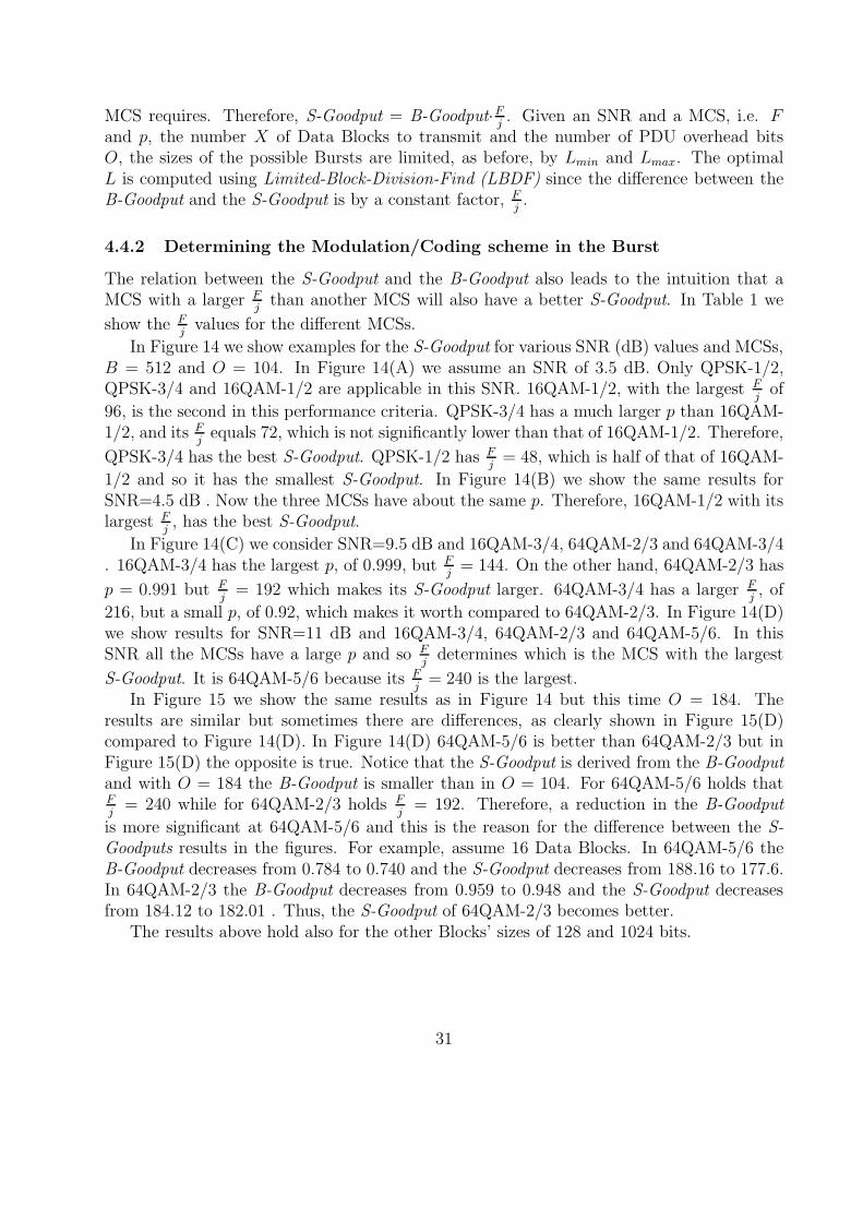
MCS requires. Therefore, S-Goodput = B-Goodput·Fj. Given an SNR and a MCS, i.e. F

and p, the number X of Data Blocks to transmit and the number of PDU overhead bitsO, the sizes of the possible Bursts are limited, as before, by Lmin and Lmax. The optimalL is computed using Limited-Block-Division-Find (LBDF) since the difference between theB-Goodput and the S-Goodput is by a constant factor, F

j.


The relation between the S-Goodput and the B-Goodput also leads to the intuition that aMCS with a larger F

jthan another MCS will also have a better S-Goodput. In Table 1 we

show the Fjvalues for the different MCSs.

In Figure 14 we show examples for the S-Goodput for various SNR (dB) values and MCSs,B = 512 and O = 104. In Figure 14(A) we assume an SNR of 3.5 dB. Only QPSK-1/2,QPSK-3/4 and 16QAM-1/2 are applicable in this SNR. 16QAM-1/2, with the largest F

jof

96, is the second in this performance criteria. QPSK-3/4 has a much larger p than 16QAM-1/2, and its F

jequals 72, which is not significantly lower than that of 16QAM-1/2. Therefore,

QPSK-3/4 has the best S-Goodput. QPSK-1/2 has Fj= 48, which is half of that of 16QAM-

1/2 and so it has the smallest S-Goodput. In Figure 14(B) we show the same results forSNR=4.5 dB . Now the three MCSs have about the same p. Therefore, 16QAM-1/2 with itslargest F

j, has the best S-Goodput.

In Figure 14(C) we consider SNR=9.5 dB and 16QAM-3/4, 64QAM-2/3 and 64QAM-3/4. 16QAM-3/4 has the largest p, of 0.999, but F

j= 144. On the other hand, 64QAM-2/3 has

p = 0.991 but Fj= 192 which makes its S-Goodput larger. 64QAM-3/4 has a larger F

j, of

216, but a small p, of 0.92, which makes it worth compared to 64QAM-2/3. In Figure 14(D)we show results for SNR=11 dB and 16QAM-3/4, 64QAM-2/3 and 64QAM-5/6. In thisSNR all the MCSs have a large p and so F

jdetermines which is the MCS with the largest

S-Goodput. It is 64QAM-5/6 because its Fj= 240 is the largest.

In Figure 15 we show the same results as in Figure 14 but this time O = 184. Theresults are similar but sometimes there are differences, as clearly shown in Figure 15(D)compared to Figure 14(D). In Figure 14(D) 64QAM-5/6 is better than 64QAM-2/3 but inFigure 15(D) the opposite is true. Notice that the S-Goodput is derived from the B-Goodputand with O = 184 the B-Goodput is smaller than in O = 104. For 64QAM-5/6 holds thatFj= 240 while for 64QAM-2/3 holds F

j= 192. Therefore, a reduction in the B-Goodput

is more significant at 64QAM-5/6 and this is the reason for the difference between the S-Goodputs results in the figures. For example, assume 16 Data Blocks. In 64QAM-5/6 theB-Goodput decreases from 0.784 to 0.740 and the S-Goodput decreases from 188.16 to 177.6.In 64QAM-2/3 the B-Goodput decreases from 0.959 to 0.948 and the S-Goodput decreasesfrom 184.12 to 182.01 . Thus, the S-Goodput of 64QAM-2/3 becomes better.

The results above hold also for the other Blocks’ sizes of 128 and 1024 bits.

31

4.5 Comparison between the performance criteria

The Max-Bits performance criteria maximizes the number of successfully transmitted databits in a Burst. Therefore, from a single user perspective, it is the best one. However,this criteria consumes many resources because it uses many FEC Blocks. This can lead toun-fairness among users if the system resources are limited. Therefore, if the system is notoverloaded, the Max-Bits criteria is applicable. However, if the system is overloaded, theS-Goodput criteria shall be used because it uses the transmission slots in the most efficientway, as we show next.

In Figures 16 and 17 we check the following for four SNR values, different numbers ofData Blocks X , B = 512 and O = 104: Given an SNR and X , we compute the optimal Burstsize according to each of the three performance criteria. Then, for each such Burst size wecompute the number of successfully transmitted data bits, and the number of transmissionslots, that such a Burst occupies. Notice that in order to find the optimal Burst size for theB-Goodput and for the S-Goodput criteria, given an SNR and X , we check all the applicableMCSs, and choose the best among them.

From Figure 16 it turns out that using the optimal Burst sizes according to the B-Goodputand the S-Goodput criteria does not reduce significantly the average number of successfullytransmitted data bits, compared to the optimal Burst size of the Max-Bits criteria.

On the other hand, from Figure 17, one can see that the saving in the number of the trans-mission slots is very significant. Therefore, the S-Goodput is the most attractive performancecriteria to use.

We want to further elaborate on Figures 16 and Figure 17. Concerning Figure 16 allthe curves are almost the same because for almost every X and SNR the best MCS is a onewith a FEC success probability of 0.999 and so also all the PDUs’ success probabilities arevery high.

Consider for example SNR=9.5 dB and X=16. We see a small difference among thecurves. For the Max-Bits criteria we choose 16QAM-3/4 with p = 0.999 and we receive thaton average 16 · 512 · 0.999 · 0.999 = 8175 data bits are transmitted successfully ( 16 PDUsof 2 FEC Blocks each). For the B-Goodput the best MCS is QPSK-1/2 with 4 PDUs of 5FEC Blocks each. The PDU success probability is 0.995 and we receive on average 8151data bits that are transmitted successfully. For the S-Goodput the best MCS is 64QAM-2/3.Here the best way to transmit the 16 · 512 data bits is in 4 PDUs of 5 FEC Blocks each, and2 PDUs of 4 FEC Blocks each. We receive that on average 7847 data bits are transmittedsuccessfully.

On the other hand consider SNR=11 dB and again X = 16. We see a small differenceamong the curves this time. The best MCSs for the Max-Bits, B-Goodput and S-Goodputcriteria are 64QAM-3/4, 64QAM-2/3 and 64QAM-3/4 respectively. The average number ofsuccessfully transmitted data bits are 8175, 8102 and 8151 respectively.

From the two examples above it can be concluded that the similarity among the curvesof the three criteria depends on the FEC Blocks’ success probabilities of the MCSs that arethe best in the three performance criteria. When these probabilities are similar, the curvesare similar and vice versa.

32

Consider Figure 17(C) now, for SNR=9.5 dB. The curves for S-Goodput and Max-Bitsare smooth. For the Max-Bits we always choose 16QAM-3/4 because it has a FEC Block’ssuccess probability of 0.999 and it uses the less number of slots per FEC Block among allthe MCSs that have p = 0.999 in this SNR. In the S-Goodput criteria the best MCS forall X is 64QAM-2/3. Therefore, in the two above criteria the number of slots in the Burstincreases as the number of Data Blocks X increases and the curves are smooth. The curvefor the B-Goodput is not smooth and this is because the best MCS is different in the variousXs. From X = 4 up to X = 24 the best MCS is sometimes QPSK-1/2 and sometimesQPSK-3/4. The best MCS is derived from the relation between the size of the FEC Block Fand X ·B and on how many free bits remain ( see section 4.3.2 ). Both MCSs have p = 0.999in this MCS so this is not a differentiating parameter in this case. For X = 6, 8, 10, 16, 22QPSK-1/2 is the best MCS and for X = 4, 12, 14, 18, 20, 24 QPSK-3/4 is the best MCS.Recall that for QPSK-1/2 holds j = 10 and for QPSK-3/4 holds j = 6. Therefore, for all theXs where QPSK-1/2 is used the number of slots in the Burst ”jumps” significantly whilewhen QPSK-3/4 is used the number of slots becomes smaller significantly.

The above results hold for O = 184 and B = 128, 1024 as well.

5 Summary of results and Conclusions

In this paper we solve several scheduling problems related to the mutual influence between thePHY layer budding blocks (FEC Blocks) and the MAC level allocations, i.e. the transmissionof MAC level packets denoted Protocol Data Units (PDUs). We look on a special case ofthe problem where Application packets are divided into equal length Data Blocks and PDUscontain an integral number of Data Blocks.

In the first stage we solve two problems in which we are given a Burst. In the firstproblem we look for the most efficient use of the given Burst, and the number of DataBlocks is not limited. This criteria is denoted Burst-Goodput (B-Goodput). In the secondproblem we show how to use the given Burst in the most efficient way, given a number ofData Blocks to transmit. This criteria is denoted Data-Goodput(D-Goodput). We solve thesetwo problems using Dynamic Programming algorithms. The complexity of the first solutionis O(L2B) where L is the number of the FEC Blocks in the Burst, and B is the length, inbits, of a Data Block. This holds for the case F < 2B − 1 where F is the length of a FECBlock in bits. Otherwise, the complexity is O(L2F ). The complexity of the second solutionis O(L ·F ·X2) where X is the given number of Data Blocks. Thus, the two algorithms havea polynomial run time complexity in the number of Data Blocks in use, and the number ofFEC Blocks, and exponential in the FEC Blocks and Data Blocks sizes.

We found that given the Signal-to-Noise-Ratio (SNR) of the channel, choosing an ap-propriate Modulation/Coding scheme (MCS) results with high B-Goodput and D-Goodputdespite the use in Data Blocks. As a rule of thumb, the best MCS to choose in relation tothe B-Goodput is the one that maximizes the PDU success probability. In relation to theD-Goodput, if the number of Data Blocks is small, the same conclusion holds. Otherwise,the best MCS is the most reliable one that also enables to transmit all the Data Blocks in

33

the Burst.In the second stage we look on a model where we are given a number of Data Blocks

to transmit, and we look for the optimal Burst size to transit these Data Blocks, accordingto three possible performance criteria: The first criteria, Max-Bits, maximizes the numberof successfully transmitted data bits in the Burst. The second criteria, Burst-Goodput,maximizes the ratio between the number of successfully transmitted data bits in the Burst,to the Burst size. The third criteria, Slot-Goodput, maximizes the number of successfullytransmitted data bits per transmission slot.

We find that when the network is overloaded, i.e. there is a high Demand for transmissiontime, the SlotGoodput criteria shall be used because it uses the transmission slots, andtherefore the physical resources, most efficiently. On the other hand, we show that thenumber of successfully transmitted data bits is not significantly lower than that in the Max-Bits criteria. When the demand for transmission time is low one shall use the Max-Bitsperformance criteria because from the point of view of a single client, this is the performancecriteria that gives the best performance.

References

[1] IEEE Standard for Local and Metropolitan Area Networks. IEEE 802.16e, Part 16: AirInterface for Fixed and Mobile Broadband Wireless Access Systems, June 2005.

[2] F. H. Huang, ”Evaluation of Soft Output Decoding for Turbo Codes”,M.Sc. Thesis, EE Faculty, Virginia Polytechnic Institute, May, 1997 ;http://scholar.lib.vt.edu/theses/available/ edt-71897-15815/unrestricted.

[3] Y. Alpert, J. Segev, O. Sharon, ”Towards an optimal transmission of SDUs in IEEE802.16 WiMAX systems”, Physical Communication 3(2013) pp. 44-60

[4] WiMAX ForumTM Mobile Radio Conformance Tests (MRCT) , Release 1.0 . ApprovedSpecification ( Revision 2.2.0 )

[5] C. So-In, R. Jain, A.K. Tamimi, ”Scheduling in IEEE 802.16e Mobile WiMAX Networks:Key Issues and a Survey”, in IEEE Journal on Selected Areas in Communication, Feb.2009, Vol. 27, No. 2

[6] E. Modiano, ”An Adaptive Algorithm for Optimizing the Packet Size used in WirelessARQ Protocols”, in ACM-Baltzer Journal of Wireless Networks 5, pp. 279-286, 1999

[7] S. Sarkar, F. M. Anjum, R. Jain, ” Throughput Optimal Packet Size Selection (TOPS)for Bluetooth Networks”, in Proc. of Int. Teletraffic Congress (ITC 18), Berlin, Ger-many, Sept. 2003, pp. 151-160

[8] Y. Fakhri, B. Nsiri, D. Aboutajdine, J. Vidal, ” Throughput Optimization Via thePacket Length and Transmission Rate For Wireless OFDM Systems in Downlink Trans-

34

mission”, in Int. Journal of Computer Science and Network Security, Vol. 6, No. 3B,March 2006, pp. 41-46

[9] A. Nandi, S. Kundu, ”Energy Level Performance and Optimum Packet Size in WirelessSensor Networks in Presence of Rayleigh Fading”, in Sensors & Transducers Journal,Vol. 118, Issue 7, July 2010, pp. 59-72

[10] P. Arlos, M. Fiedler, ” Influence of the Packet Size on the One-Way Delay in 3GNetworks”, in 11th Int. Conf. Passive and Active Measurements (PAM 2010), pp. 61-70

[11] M. N. Krishnan, E. Haghani, A. Zakhor, ”Packet Length Adaptation in WLANs withHidden Nodes and Time-Varying Channels”, in Submitted Globecom 2011

[12] Y. Sankarasubramaniam, I. F. Akyildiz, S. W. McLaughlin, ” Energy Efficiency basedPacket Size Optimization in Wireless Sensor Networks”, in Int. Workshop on SensorNetwork Protocols and Applications, 2003, pp. 1-8

[13] C. K. Siew, D. J. Goodman, ” Packet Data Transmission Over Mobile Radio Channels”,in IEEE Transactions on Vehicular Technology, Vol. 38, No. 2, May 1989

[14] I. Ahmad, D. Hqabibi, ” A Novel Mobile WiMAX Solution for Higher Throughput”, inInt. Conf. on Networks (ICON), 2008, pp. 1-5

[15] J.Y. Choi, K.P. Choi, J. Shin, ”Mathematical Analysis of H.264 Video Error-Controlon Cross-Layer Framework”, in The 21st Int. Technical Conf. on Circuits/Systems,Computers and Communications, 2006, pp. III-45 - III-48

[16] U. Mudugamuwa, M. Karaliopoulos, R. Tafazolli, B. G. Evans, ”Impact of packet-levelFEC and outer block interleaving on MBMS delivery over WCDMA mobile satellitesystems”, in The 6th European Mobile Personal Satellite Communication Workshop(EMPS), 2004

[17] A. Basalamah, T. Sato, ”Adaptive FEC Reliable Multicast MAC Protocol for WLAN”,in IEEE 66th Vehicular Technology Conf. (VTC), 2007, pp. 244-248

[18] M. Bykowski, K. Kowalik, B. Keegan, M. Davis, ”Throughput Enhancement throughCombined Fragmentation and Rate Method in IEEE 802.11b WLANs”, in Workshop onWireless Broadband Access for Communities and Rural Developing Regions (Wireless),2008

[19] M. Emmelmann, H. Bischl, ”An Adaptive MAC Layer Protocol for ATM-based LEOSatellite Networks (Extended Abstract)”, in IEEE 58th Vehicular Technology Conf.(VTC), 2008, pp. 2698-2702

35

[20] M. C. Vuran, I. F. Akyildiz, ”Cross-layer Packet Size Optimization for Wireless Ter-restrial, Underwater, and Underground Sensor Networks”, in INFOCOM 2008, pp.226-230

[21] S. Choi, Y. Choi, I. Lee, ”IEEE 802.11 MAC-Level FEC Scheme with RetransmissionCombining”, in IEEE Trans. on Wireless Communication, Vol. 5, Nu. 1, Jan 2006,pp.203-211

[22] W. Chaohui, L. Yuhong, H. Li, M. Jian, ”A New Reliable Multicast Scheme for Mul-timedia Applications in Wireless Environment”, in IEEE 2nd Int. Conf. on BroadbandNetworks & Multimedia Technology, 2009, pp. 744-748

[23] Y. Chang, C. Lee, B.K. Kwon, J. A. Copeland, ”Dynamic Optimal Fragmentation withRate Adaptation for Goodput Enhancement in WLANs”, in International Conferenceon Wireless Networks (ICWN), June 2007

[24] P. Lettieri, B. Srivastava, ”Adaptive Frame Length Control for Improving Wireless LinkThroughput, Range and Energy Efficiency”, in INFOCOM 1998, pp. 564-571

[25] A. Bestetti, G. Giambene, S. Hadzic, ”Fair Traffic Scheduling for WiMAX Systems”, in6th Int. Conf. on Symposium on Wireless Communication Systems, Siena, Italy, 2009,pp. 254-258

[26] A. Bestetti, G. Giambene, S. Hadzic, ”WiMAX: MAC Layer Performance Assessments”,in 3rd International Symposium on Wireless Pervasive Computing (ISWPC) 2008

[27] A. Sayenko, O. Alanen, J. Karhula, T. Hamaainen, ”Ensuring the QoS requirements in802.16 Scheduling”, in Proc. Int. Workshop Modeling Analysis and Simulation Wirelessand Mobile Systems, Terromolinos, Spain, 2006, pp. 108-117

[28] A. Sayenko, O. Alanen, T. Hamaainen, ”Scheduling solution for the IEEE 802.16 basestation”, in Int. J. Computer and Telecommunications Networkink, Jan. 2008, Vol. 52,pp. 96-115

[29] A. Tanenbaum, ”Computer Networks”, Fourth Edition, Prentice Hall

[30] B. H. Kim, J. Yun, Y. Hur, ”Capacity Estimation on TCP Performance Enhancementover Mobile WiMAX Networks”, in IEEE Communication Magazine, June 2009, Vol.47, Issue 6, pp. 132-141

[31] C. Cicconetti, L. Lenzii, E. Mingozzi, C. Eklund, ”Quality of service support in IEEE802.16 networks”, in IEEE Network, April 2006, Vol. 20, pp. 50-55

[32] C. Cicconetti, A. Erta, L. Lenzii, E. Mingozzi, ”Performance Evaluation of the IEEE802.16 MAC for QoS Support”, in IEEE Trans. Mobile Comput., Nov. 2006, Vol. 6,pp. 26-38

36

[33] J. Chen, W. Jiao, H. Wang, ”A service flow management strategy for IEEE 802.16broadband wireless access systems in TDD mode”, in Proc. IEEE Int. Conf. Commu-nications, Seoul, Korea, 2005, Vol. 5, pp. 3422-3426

[34] J. Jin, B. Li, ”Adaptive Random Network Coding in WiMAX”, in ICC 2008, Beijing,China

[35] J. J. Lee, M. Goel, Y. Zhu, J. F. Ren, Y. Sun, ”Forward Error Correction Decoding forWiMAX and 3GPP LTE Modems”, in 42nd Asilomar Conf. on Signals, Systems andComputers, Pasific Grove, CA, USA, Oct. 2008

[36] L. Zhang, P. Senac, R. Boreli, M. Diaz, ”Optimization of WiMAX modulation schemewith cross layer erasure node”, in WOEMOM 2009, Kos, Greece

[37] L. Lin, W. Jia, W. Lu, ”Performance Analysis of IEEE 802.16 Multicast and Broad-cast Polling based Bandwidth Request”, in Proc. IEEE Wireless Communication andNetworking Conf., Hong Kong, 2007, pp. 1854-1859

[38] S. Sengupta, M. Chatterjee, S. Ganguly, ”Improving Quality of VoIP Streams overWiMAX”, in IEEE Trans. Comput., Feb. 2008, Vol. 57, pp. 145-156

[39] S. Sengupta, M. Chatterjee, S. Ganguly, R. Izmailov, ”Exploiting MAC Flexibility inWiMAX for Media Streaming”, in WOWMOM 2005, Naxos, Greece, pp. 338-343

[40] V. Singe, V. Sharma, ”Efficient and Fair Scheduling of Uplink and Downlink in IEEE802.16 OFDMA Networks”, in Proc. IEEE Wireless Communication and NetworkingConf., Las Vegas, NV, 2006, Vol. 2, pp. 984-990

[41] V. Tykhomyvov, A. Sayenko, H. Martikainen, O. Alanen, T. Hamalainen, ”PerformanceEvaluation of the IEEE 802.16 ARQ Mechanism”, in 7th International Conf. on NextGeneration Teletraffic and Wired/Wireless Advanced Networking, Sept. 2007, pp. 148-161.

[42] E. Halepovic, Q. Wu, C. Williamson, M. Ghadevi, ”TCP over WiMAX: A MeasurmentStudy”, in IEEE/ACM MASCOT 2008, Baltimore, MD, USA

[43] Y. A. Sekercioglu, M. Ivanovich, A. Yegin, ”A Survey of MAC based QoSimplementation for WiMAX networks”, in Computer Networks, 2009, doi:10.1016/j.comnet.2009.05.001

Y. A. Sekercioglu, M. Ivanovich, A. Yegin, ”A Survey of MAC based QoSimplementation for WiMAX networks”, in Computer Networks, 2009, doi:10.1016/j.comnet.2009.05.001

[44] H. Martikainen, A. Sayenko, O. Alanen, V. Tykhomyrov, ”Optimal MAC PDU Size inIEEE 802.16”, in Telecommunication Networking Workshop on QoS in Multiservice IPNetworks, Venice, Italy, 2008, pp. 66-71

37

[45] Y. Alpert, J. Segev, O. Sharon, ”Advanced coupled PHY and MAC scheduling in IEEE802.16 WiMAX systems”, in Physical Communication 3(2010) pp. 287-298

[46] Y. Alpert, J. Segev, O. Sharon, ”Coupled PHY, MAC and Repetiton in IEEE 802.16WiMAX systems”, in Physical Communications 7(2013) pp. 14-29

[47] O. Sharon, G. TabaJha, Y. Alpert, ”Efficient Coupled PHY and MAC use of PhysicalBursts in WiMAX/IEEE 802.16e Networks”, in Physical Communications 7(2013) pp.73-91

[48] O. Sharon, Y. Alpert, ”PHY and MAC criterion for Optimal MAC PDU size in ARQ-Enabled connections in WiMAX/IEEE 802.16e Networks”, Accepted, InternationalJournal of Communication Systems

[49] A. Allahverdi, C. T. Ng, T.C.E. Cheng, M. Y. Kovalyov, ”A survey of schedulingproblems with setup times or costs”, European Journal of Operational Research 187(2008) pp. 985-1032

[50] Xu Jun, ZTE Corporation, China (http://wwwen.zte.com.cn), Personal communication

38

Figure 5: The D-Goodput for various SNRs, Data Blocks’ sizes and Bursts’ sizes

39

Figure 6: The maximum number of Data Blocks in different Data Blocks’ sizes and Bursts’sizes

Figure 7: The D-Goodputs in the ’QPSK-1/2 saturated’ and the ’QPSK-3/4 saturated’scenarios

40

Figure 8: Allocating PDUs over FEC Blocks

41

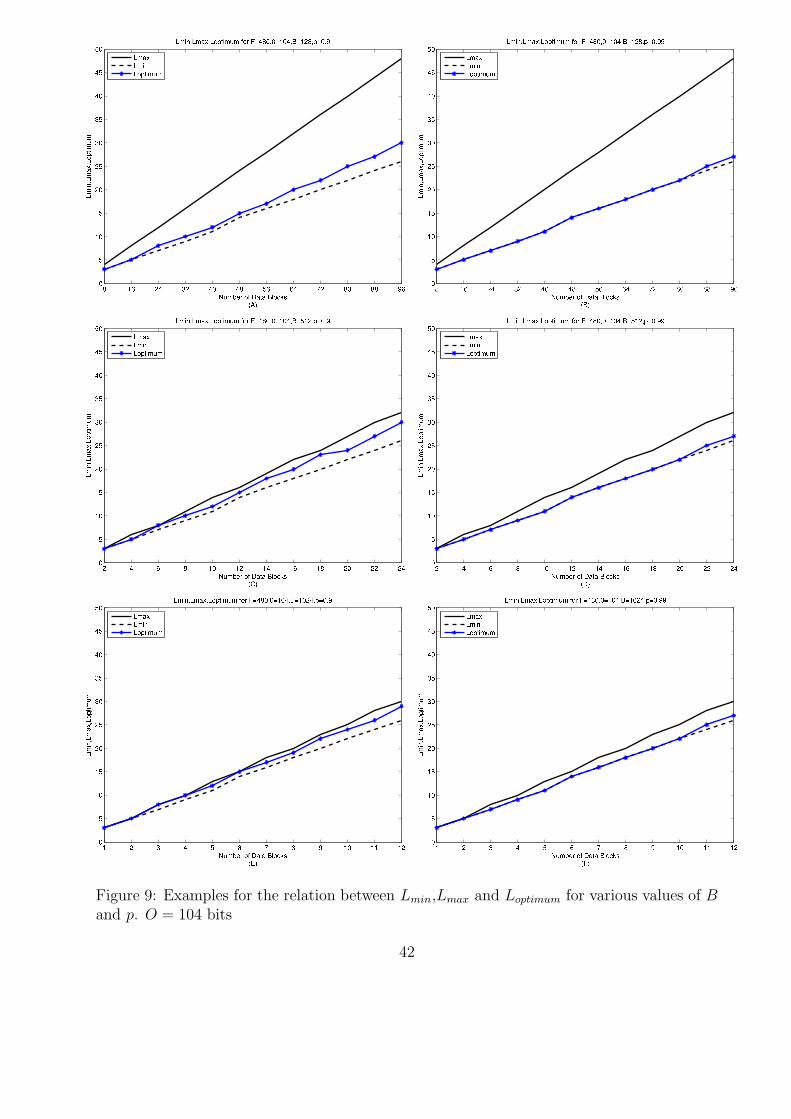
Figure 9: Examples for the relation between Lmin,Lmax and Loptimum for various values of Band p. O = 104 bits

42

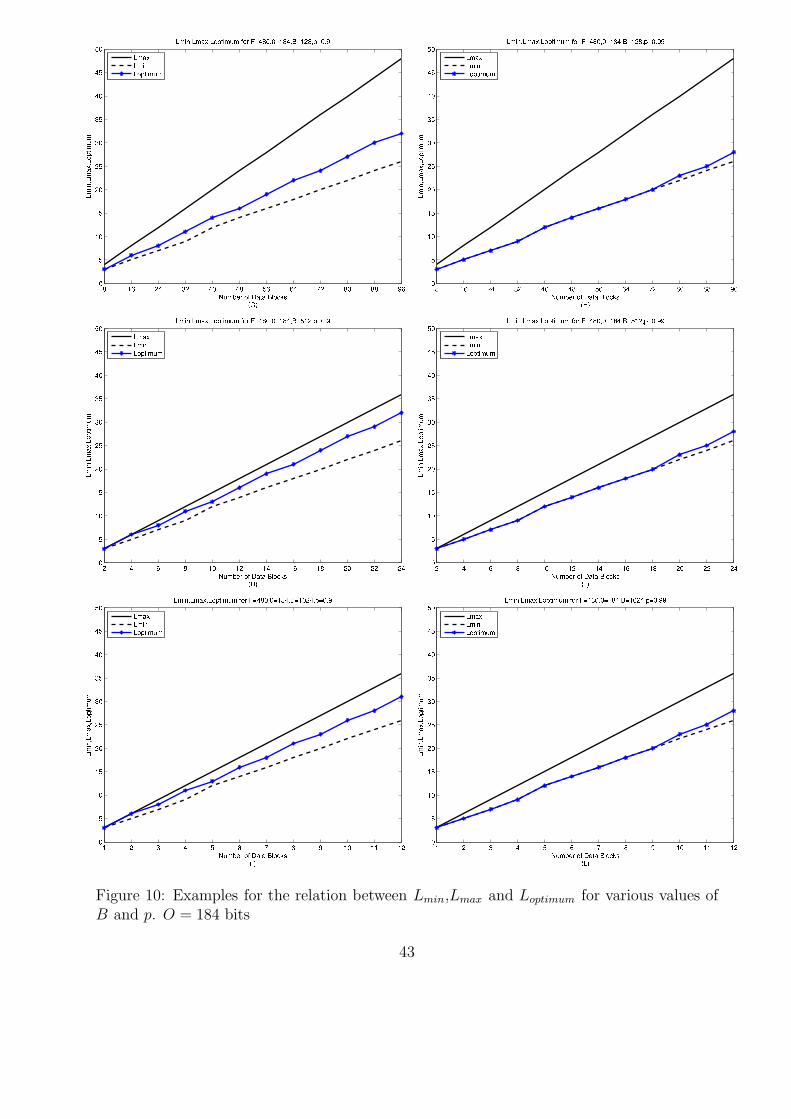
Figure 10: Examples for the relation between Lmin,Lmax and Loptimum for various values ofB and p. O = 184 bits

43

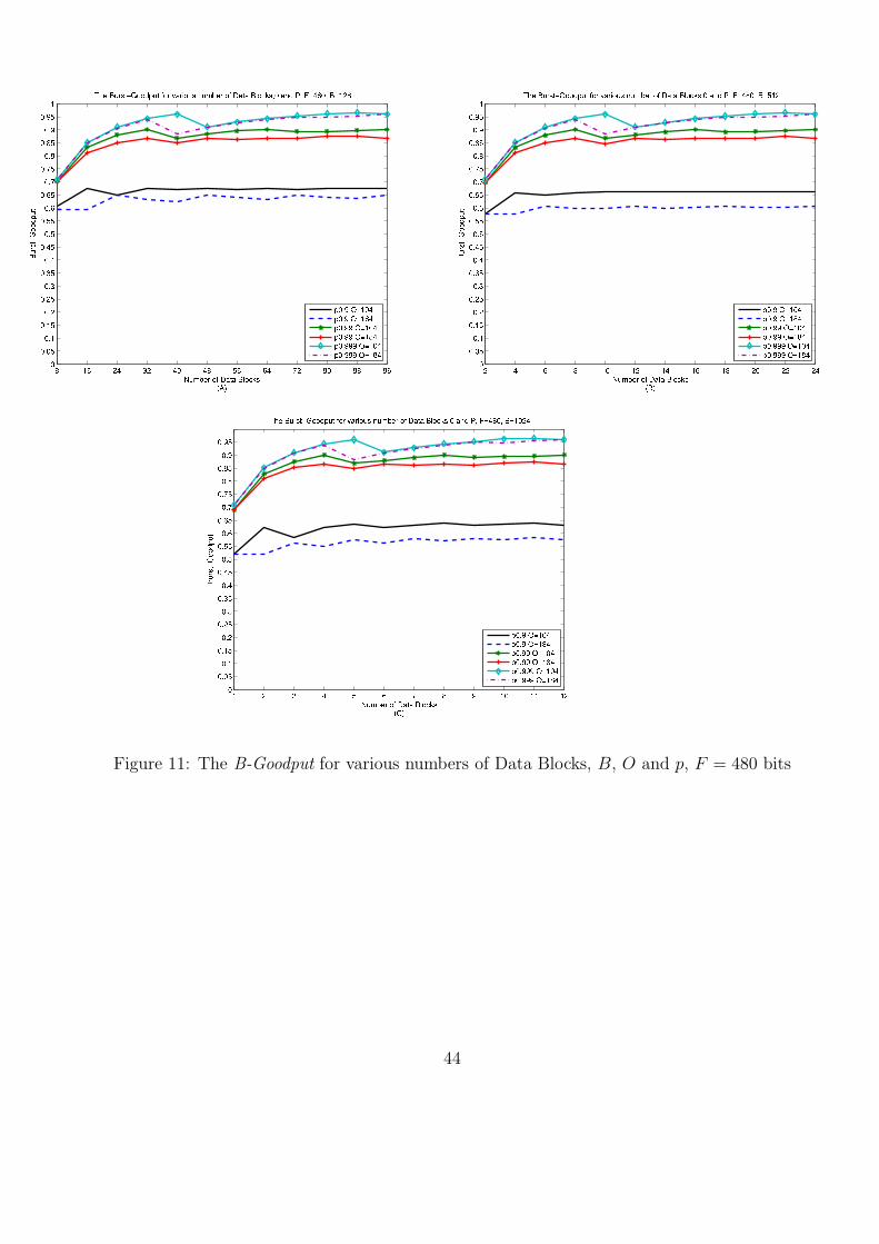
Figure 11: The B-Goodput for various numbers of Data Blocks, B, O and p, F = 480 bits

44

Figure 12: The B-Goodput in various MCSs and SNRs (dB) and for various numbers of DataBlocks. B = 512, O = 104 bits

45

Figure 13: The B-Goodput in various MCSs and SNRs (dB) and for various numbers of DataBlocks. B = 512, O = 184 bits

46

Figure 14: The S-Goodput in various MCSs and SNRs (dB) and for various numbers of DataBlocks, B = 512, O = 104 bits

47

Figure 15: The S-Goodput in various MCSs and SNRs (dB) and for various numbers of DataBlocks, B = 512, O = 184 bits

48

Figure 16: The average number of successfully transmitted data bits in the optimal Burstsize of the various performance criteria, for various SNRs (dB) and for various numbers ofData Blocks, B = 512, O = 104 bits

49

Figure 17: The number of slots in the optimal Burst size of the various performance criteria,for various SNRs (dB) and for various numbers of Data Blocks, B = 512, O = 104 bits

50

Table 1: The number of slots j, the number of data bits F and the success probability p invarious SNR values (dB) of the largest FEC block in various MCSs

MCS j F Fj

SNR (dB)

2 2.5 3 3.5 4 4.5 5 5.5 6

QPSK 1/2 10 480 48 0.998 0.999 0.999 0.999 0.999 0.999 0.999 0.999 0.999

QPSK 3/4 6 432 72 0.38 0.85 0.96 0.998 0.999 0.999 0.999 0.999 0.999

16QAM-1/2 5 480 96 * * 0.43 0.82 0.976 0.998 0.999 0.999 0.999

16QAM-3/4 3 432 144 * * * * * * 0.42 0.79 0.957

64QAM-2/3 2 384 192 * * * * * * * * *

64QAM-3/4 2 432 216 * * * * * * * * *

64QAM-5/6 2 480 240 * * * * * * * * *

MCS SNR

6.5 7 7.5 8 8.5 9 9.5 10 10.5 11 11.5 12

QPSK 1/2 0.999 0.999 0.999 0.999 0.999 0.999 0.999 0.999 0.999 0.999 0.999 0.999

QPSK 3/4 0.999 0.999 0.999 0.999 0.999 0.999 0.999 0.999 0.999 0.999 0.999 0.999

16QAM-1/2 0.999 0.999 0.999 0.999 0.999 0.999 0.999 0.999 0.999 0.999 0.999 0.999

16QAM-3/4 0.995 0.999 0.999 0.999 0.999 0.999 0.999 0.999 0.999 0.999 0.999 0.999

64QAM-2/3 * * * 0.56 0.79 0.941 0.991 0.999 0.999 0.999 0.999 0.999

64QAM-3/4 * * * 0.33 0.46 0.73 0.92 0.990 0.999 0.999 0.999 0.999

64QAM-5/6 * * * * * 0.3 0.41 0.45 0.8 0.959 0.994 0.999

51

Table 2: The number of slots j, the number of data bits F and the B-Goodput in variousMCSs and SNR values, for the case S = 900 slots, B = 128 bits and O = 104 bits

MCS j F SNR

2 2.5 3 3.5 4 4.5 5 5.5 6

QPSK 1/2 10 480 0.957 0.969 0.969 0.969 0.969 0.969 0.969 0.969 0.969

QPSK 3/4 6 432 0.225 0.589 0.791 0.955 0.969 0.969 0.969 0.969 0.969

16QAM-1/2 5 480 * * 0.254 0.548 0.847 0.957 0.970 0.970 0.970

16QAM-3/4 3 432 * * * * * * 0.249 0.511 0.781

64QAM-2/3 2 384 * * * * * * * * *

64QAM-3/4 2 432 * * * * * * * * *

64QAM-5/6 2 480 * * * * * * * * *

MCS SNR

6.5 7 7.5 8 8.5 9 9.5 10 10.5 11 11.5 12

QPSK 1/2 0.969 0.969 0.969 0.969 0.969 0.969 0.969 0.969 0.969 0.969 0.969 0.969

QPSK 3/4 0.969 0.969 0.969 0.969 0.969 0.969 0.969 0.969 0.969 0.969 0.969 0.969

16QAM-1/2 0.970 0.970 0.970 0.970 0.970 0.970 0.970 0.970 0.970 0.970 0.970 0.970

16QAM-3/4 0.969 0.969 0.969 0.969 0.969 0.969 0.969 0.969 0.969 0.969 0.969 0.969

64QAM-2/3 * * * 0.373 0.527 0.741 0.897 0.967 0.967 0.967 0.967 0.967

64QAM-3/4 * * * 0.196 0.273 0.453 0.911 0.920 0.969 0.969 0.969 0.969

64QAM-5/6 * * * * * 0.172 0.241 0.267 0.519 0.800 0.925 0.970

52

Table 3: The number of slots j, the number of data bits F and the average integral number ofsuccessfully transmitted Data Blocks in various MCSs and SNR values, for the case S = 900slots, B = 128 bits and O = 104 bits

MCS j F SNR

2 2.5 3 3.5 4 4.5 5 5.5 6

QPSK 1/2 10 480 323 327 327 327 327 327 327 327 327

QPSK 3/4 6 432 114 298 400 483 490 490 490 490 490

16QAM-1/2 5 480 * * 172 370 572 646 655 655 655

16QAM-3/4 3 432 * * * * * * 252 517 790

64QAM-2/3 2 384 * * * * * * * * *

64QAM-3/4 2 432 * * * * * * * * *

64QAM-5/6 2 480 * * * * * * * * *

MCS SNR

6.5 7 7.5 8 8.5 9 9.5 10 10.5 11 11.5 12

QPSK 1/2 327 327 327 327 327 327 327 327 327 327 327 327

QPSK 3/4 490 490 490 490 490 490 490 490 490 490 490 490

16QAM-1/2 655 655 655 655 655 655 655 655 655 655 655 655

16QAM-3/4 981 981 981 981 981 981 981 981 981 981 981 981

64QAM-2/3 * * * 503 711 1000 1210 1305 1305 1305 1305 1305

64QAM-3/4 * * * 297 414 687 1383 1410 1471 1471 1471 1471

64QAM-5/6 * * * * * 290 406 451 875 1350 1560 1636

53

6 Appendix

6.1 The code of algorithm Division-Find

We introduce a version of Algorithm Division-Find that computes the maximum B-Goodputand an optimal division of the Burst, which contains the maximum number of Data Blocks.The code only considers the case F > 2B − 1. The extension for the case F ≤ 2B − 1 istrivial. The code of the algorithm uses a procedure called FillRow which fills rows 2,.....,L inTable T. Every entry E in T contains the maximum number of succesfully transmitted databits in the Burst section starting from E up to the end of the Burst. The entry also containsthe number of Data Blocks in the PDU starting at E ( if any ), the maximum number oftransmitted Data Blocks in the Burst section from E up to the end of the Burst, and pointersto the next PDU in the division.

Procedure FillRow uses two other procedures, FillToStartingEdges and Fill-ToEndingEdges that check all the possibilities to end PDUs at the Starting and Endingedges of FEC Blocks respectively. Finally, another procedure, GetOptimalResult, is used toestablish the optimal division and it returns this division and the maximum B-Goodput.

54

Algorithm Division-Find

Input:Infinite number of Data BlocksB: size of a Data Block ( bits )F: size of a FEC Block ( bits )O: size of a PDU overhead ( bits )L: number of FEC Blocks

Output:The maximum B-Goodput, Number of Data Blocks in use, PDUs’ arrangement

Compute:

/*Every entry E in T contains the following fields:Bits - The maximum possible number of successfully transmitted data bits

from position E in the Burst up to the end of the BurstNumOfDataBlocks - The number of Data Blocks in the PDU that starts at ETotalNumOfDataBlocks - The maximum number of transmitted Data Blocks from E up to the end of the Burst(NextRow,NextCol) - Pointers to the next PDU in the Burst ( entry in T )*/

/* Check Input */1. if (2B-1>F) return ERROR

2. If (L=1) then2.1 NumOfBlocks=

⌊

F−OB

⌋

2.2 Bits=NumOfBlocks·B·p2.3 return( B-Goodput= Bits

F, TotalNumOfBlocks=NumOfBlocks,

One PDU of NumOfBlocks Data Blocks in the FEC Block )

/* Initializing step */

3. Initialize Table T with ’NIL’

/* Filling row 1 in Table T */

4. for j=1 to B do

4.1 NumOfBlocks =⌊

F−(j−1)−O

B

⌋

4.2 T[1,j].Bits=NumOfBlocks·B·p4.3 T[1,j].NumOfDataBlocks=NumOfBlocks4.4 T[1,j].TotalNumOfDataBlocks=NumOfBlocks

/* Filling rows 2 to (L-1) in Table T */

5. EndingEdgeStartBit=(F-(B-2))6. EndingEdgeEndBit= F7. StartingEdgeEndBit=B8. for (FecNumber=2) to (L-1) do8.1 FillRow(EndingEdgeStartBit,

EndingEdgeEndBit,StartingEdgeEndBit, FecNumber)

55

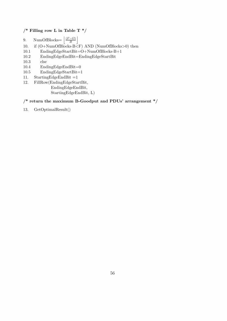
/* Filling row L in Table T */

9. NumOfBlocks=⌊

(F−O)B

⌋

10. if (O+NumOfBlocks·B<F) AND (NumOfBlocks>0) then10.1 EndingEdgeStartBit=O+NumOfBlocks·B+110.2 EndingEdgeEndBit=EndingEdgeStartBit10.3 else10.4 EndingEdgeEndBit=010.5 EndingEdgeStartBit=111. StartingEdgeEndBit =112. FillRow(EndingEdgeStartBit,

EndingEdgeEndBit,StartingEdgeEndBit, L)

/* return the maximum B-Goodput and PDUs’ arrangement */

13. GetOptimalResult()

56

ProcedureFillRow(EndingEdgeStartBit, EndingEdgeEndBit,StartingEdgeEndBit,FecNumber)

/* Compute Ending edge */

1. for j=EndingEdgeStartBit to EndingEdgeEndBit do1.1 T[FecNumber,j].Bits=TFecNumber-1,1].Bits1.2 T[FecNumber,j].NumOfDataBlocks=01.3 T[FecNumber,j].TotalNumOfDataBlocks=T[FecNumber-1,1].TotalNumOfDataBlocks1.4 T[FecNumber,j].NextRow=FecNumber-11.5 T[FecNumber,j].NextCol=11.6 FillToStartingEdges[j,FecNumber]1.7 FillToEndingEdges[j,FecNumber]

/* Compute Starting edge */

2. for j=1 to StartingEdgeEndBit do2.1 T[FecNumber,j].Bits=TFecNumber-1,1].Bits2.2 T[FecNumber,j].NumOfDataBlocks=02.3 T[FecNumber,j].TotalNumOfDataBlocks=T[FecNumber-1,1].TotalNumOfDataBlocks2.4 T[FecNumber,j].NextRow=FecNumber-12.5 T[FecNumber,j].NextCol=12.6 FillToStartingEdges[j,FecNumber]2.7 FillToEndingEdges[j,FecNumber]

57

Procedure FillToStaringEdges(j,FecNumber)1. for i=1 to (FecNumber-1) do


(F−(j−1))+F ·(i−1)+(B−1)−O

B

⌋

1.2 EndingPduBit=((j-1)+O+NumOfBlocks·B mod F1.3 if (NumOfBlocks>0) AND (EndingPduBit>0) AND (EndingpduBit<B) then1.3.1 NextRow=FecNumber-11.3.2 NextCol=(EndingPduBit+1)1.3.3 NextTotalNumOfBlocks=T[NextRow,NextCol].TotalNumOfDataBlocks1.3.4 Bits=NumOfDataBlocks·B·pi+1+T[NextRow,NextCol].Bits1.3.5 if (Bits>T[FecNumber,j].Bits) OR

((Bits=T[FECNumber,j].bits) AND(NumOfBlocks+NextTotalNumOfBlocks>T[fecNumber,j].TotalNumOfDataBlocks))

then1.3.5.1 T[FecNumber,j].Bits=Bits1.3.5.2 T[FecNumber,j].NumOfDataBlocks=NumOfDataBlocks1.3.5.3 T[FecNumber,j].TotalNumOfDataBlocks=NumOfBlocks+NextTotalNumOfDataBlocks1.3.5.4 T[FecNumber,j].NextRow=NextRow1.3.5.5 T[FecNumber,j].NextCol=NextCol

Procedure FillToEndingEdges(j,FecNumber)1. for i=1 to FecNumber do1.1 if (j>B) AND (i=1) continue


(F−(j−1))+F ·(i−1)−O

B

⌋

1.3 if (NumOfBlocks>0) then1.3.1 NextRow=FecNumber-(i-1)1.3.1 NextCol= ((j-1)+(O+NumOfBlocks·B)+1) mod F1.3.2 if (NextCol=0) then NextCol=F1.3.3 if (NextCol=1) AND (NextRow=1) then1.3.3.1 NextPduBits=01.3.3.2 NextTotalNumOfDataBlocks=01.3.3.3 else1.3.3.4 if (NextCol=1) AND (NextRow>1) then1.3.3.4.1 NextRow=NextRow-11.3.3.4.2 NextPduBits = T[NextRow,NextCol].Bits1.3.3.4.3 NextTotalNumOfDataBlocks=T[NextRow,NextCol].TotalNumOfDataBlocks1.3.4 Bits=NumOfBlocks·B·i+NextPduBits1.3.5 if (Bits>T[FecNumber,j].Bits) OR

((Bits=T[FECNumber,j].bits) AND(NumOfBlocks+NextTotalNumOfBlocks>T[fecNumber,j].TotalNumOfDataBlocks))

then1.3.5.1 T[FecNumber,j].Bits=Bits1.3.5.2 T[FecNumber,j].NumOfDataBlocks=NumOfDataBlocks1.3.5.3 T[FecNumber,j].TotalNumOfDataBlocks=NumOfBlocks+NextTotalNumOfDataBlocks1.3.5.4 T[FecNumber,j].NextRow=NextRow1.3.5.5 T[FecNumber,j].NextCol=NextCol

58

Procedure GetOptimalResult returns the maximum B-Goodput and the optimal division of theBurst. The optimal B-Goodput and the maximum number of Data Blocks in an optimal division arereturned in the variables B−Goodput and NumOfDataBlocksInTheOptimalBGoodput respectively.The optimal dividion is kept in an array named PDU, in which every entry represents a PDU. Everyentry contains the number of Data Blocks in the PDU and a flag indicating whether the PDU beginsat the beginning of a FEC Block or whether it is loctaed B2B with the previous one.

Procedure GetOptimalResult

1. B-Goodput=T[L,1].Bits / (F·L)2. NumOfDataBlocksInTheOptimalBGoodput=T[L,1].TotalNumOfDataBlocks3. NumOfPdus = 04. Row=L ; Col= 15. While(true)5.1 NumOfPdus++5.2 PDU[NumOfPdus].NumOfDataBlocks=T[Row,Col].NumOfDataBlocks5.3 if (Col=1) then5.3.1 PDU[NumOfPdus].StartAtNewFecBlock=True5.3.2 else5.3.3 PDU[NumOfPdus].StartAtNewFecBlock=False5.4 TempRow=Row5.5 Row=T[Row,Col].Row5.6 Col=T[TempRow,Col].Col5.7 if (Row!=0) AND (T[Row,Col].NumOfDataBlocks=0)5.7.1 TempRow=Row5.7.2 Row=T[Row,Col].NextRow5.7.3 Col=T[TempRow,Col].NextCol5.8 if (Row=NIL) then return(B-Goodput,NumOfDataBlocksInTheOptimalBGoodput, PDU);

59

6.2 The code of algorithm Limited-Block-Division-Find

We introduce a version of Algorithm Limited-Block-Division-Find that computes the maximumD-Goodput and an optimal division of the Burst, which contains given X Data Blocks. The tableT is now 3-D, where an entry correspondes to a position in the Burst (FEC Block and bit position)and a number d of Data Blocks that are transmitted from the position in the Bursr up to the endof the Burst. The code of the algorithm uses a procedure called FillCell which fills the entriesin rows 2,.....,L in Table T. Every entry E in T, that corresponds to the transmission of d DataBlocks, contains the maximum number of succesfully transmitted data bits in the Burst sectionstarting from E up to the end of the Burst. The entry also contains pointers to the next PDU inthe division.

Finally, another procedure, GetOptimalResult, is used to establish the optimal division and itreturns this division and the maximum D-Goodput.

60

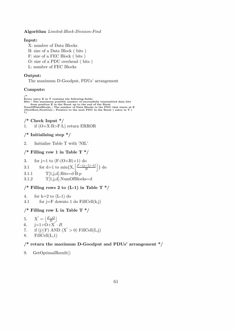
Algorithm Limited-Block-Division-Find

Input:X: number of Data BlocksB: size of a Data Block ( bits )F: size of a FEC Block ( bits )O: size of a PDU overhead ( bits )L: number of FEC Blocks

Output:The maximum D-Goodput, PDUs’ arrangement

Compute:

/*Every entry E in T contains the following fields:Bits - The maximum possible number of successfully transmitted data bits

from position E in the Burst up to the end of the BurstNumOfDataBlocks - The number of Data Blocks in the PDU that starts at E(NextRow,NextCol) - Pointers to the next PDU in the Burst ( entry in T )*/

/* Check Input */1. if (O+X·B>F·L) return ERROR

/* Initializing step */

2. Initialize Table T with ’NIL’

/* Filling row 1 in Table T */

3. for j=1 to (F-(O+B)+1) do

3.1 for d=1 to min{X,⌊

F−(j−1)−O

B

⌋

} do

3.1.1 T[1,j,d].Bits=d·B·p3.1.2 T[1,j,d].NumOfBlocks=d

/* Filling rows 2 to (L-1) in Table T */

4. for k=2 to (L-1) do4.1 for j=F downto 1 do FillCell(k,j)

/* Filling row L in Table T */

5. X′

=⌊

F−OB

⌋

6. j=1+O+X′

·B7. if (j≤F) AND (X

′

> 0) FillCell(L,j)8. FillCell(L,1)

/* return the maximum D-Goodput and PDUs’ arrangement */

9. GetOptimalResult()

61

ProcedureFillCell(k,j)

1. for d=1 to min{X,⌊

k·F−(j−1)−O

B

⌋

} do

1.1 T[k,j,d].Bits=T[k-1,1,d].Bits1.2 T[k,j,d].NumOfDataBlocks=01.3 T[k,j,d].NextRow=(k-1)1.4 T[k,j,d].NextCol=11.5 for i=1 to d do

1.5.1 PduBits=i·B·p

⌈

(j−1)+O+i·B

F

⌉

1.5.2 NextRow=k-(⌈

j+O+i·bF

⌉

-1)

1.5.3 NextCol=((j+O+i·B) mod F)1.5.4 if (NextCol=0) then NextCol=F1.5.5 NextNumOfDataBlocks= d-i1.5.6 if (NextNumOfDataBlocks != 0) then1.5.6.1 NextBits=T[NextRow,NextCol,NextNumOfDataBlocks].Bits1.5.7 else NextBits=01.5.8 if (PduBits+NextBits > T[k,j,d].Bits) then1.5.8.1 T[k,j,d].Bits=PduBits+NextBits1.5.8.2 T[k,j,d].NumOfDataBlocks= i1.5.8.3 T[k,j,d].NextRow = NextRow1.5.8.4 T[k,j,d].NextCol = NextCol

62

Procedure GetOptimalResult returns the maximum D-Goodput and the optimal division of theBurst. The optimal D-Goodput is returned in the variable D−Goodput. The optimal dividion iskept in an array named PDU, in which every entry represents a PDU. Every entry contains thenumber of Data Blocks in the PDU and a flag indicating whether the PDU begins at the beginningof a FEC Block or whether it is loctaed B2B with the previous one.

Procedure GetOptimalResult

1. D-Goodput=T[L,1,X].Bits / (X·B)2. NumOfPdus = 03. Row=L ; Col= 14. Blocks=X5. While(Blocks>0)5.1 NumOfPdus++5.2 PDU[NumOfPdus].NumOfDataBlocks=T[Row,Col,Blocks].NumOfDataBlocks5.3 if (Col=1) then5.3.1 PDU[NumOfPdus].StartAtNewFecBlock=True5.3.2 else5.3.3 PDU[NumOfPdus].StartAtNewFecBlock=False5.4 TempRow=Row5.5 Row=T[Row,Col,Blocks].NextRow5.6 Col=T[TempRow,Col,Blocks].NextCol5.7 Blocks=Blocks-PDU[NumOfPdus].NumOfDataBlocks5.8 if (Blocks>0) AND (T[Row,Col,Blocks].NumOfDataBlocks=0) then5.8.1 TempRow=Row5.8.2 Row=T[Row,Col,Blocks].NextRow5.8.3 Col=T[TempRow,Col,Blocks].NextCol6. return(D-Goodput,PDU);

63

MyThesis

Documents

wireless networks

ewimax networks

downlink of ieee

broadband access

networks fulll

mac level frames

microwave access

e systems