Mutation model for nucleotide sequences based on crystal basis

arX

iv:q

-bio

/050

6010

v1 [

q-bi

o.B

M]

8 J

un 2

005

Mutation model for nucleotide sequencesbased on crystal basis

C. Minichini , A. Sciarrino†

Dipartimento di Scienze Fisiche, Universita di Napoli “Federico II”

and †I.N.F.N., Sezione di Napoli

Complesso Universitario di Monte S. Angelo

Via Cintia, I-80126 Naples, Italy

Abstract

A nucleotides sequence is identified, in the two (four) letters alphabet, by the the labels ofa vector state of an irreducible representation of Uq→0(sl(2)) (Uq→0(sl(2) ⊕ sl(2))). A masterequation for the distribuion function is written, where the intensity of the one-spin flip is assumedto depend from the variation of the labels of the state. In the two letters approximation, thenumerically computed equilibrium distribution for short sequences is nicely fitted by a Yuledistribution, which is the observed distribution of the ranked short oligonucleotides frequencyin DNA. The four letter alphabet description, applied to the codons, is able to reproduce theform of the fitted rank ordered usage frequencies distribution.

Keywords: mutation, rank ordered distribution, codons, oligonucleotides, crystal

basis

preprint DSF 14/2005

email: [email protected] [email protected]

Corresponding author: A. Sciarrino - Tel +39-081676807 - Fax +39-081676346

1 Introduction

Mutations in DNA play a very important role in the theory of evolution. DNA and RNA are build

up as sequences of four basis or nucleotides which are usually identified by the letters: C, G, T, A

(T being replaced by U in RNA), C and U (G and A) belonging to the purine family, denoted by

R (respectively to the pyrimidine family, denoted by Y). Therefore in the case of genome sequences

each point in the sequence should be identified by an element of a four letter alphabet or by a set

of two binary values. In a simplified treatment one identifies each element according to the purine

or pyrimidine nature, reducing so to a two letter alphabet or to a binary set. Genetic mutations,

i.e. modifications of the DNA genomic sequences, play a fundamental role in the evolution. They

include changes of one or more than one nucleotide, insertions and deletions of nucleotides, frame-

shifts and inversions. In the present paper we consider only the point mutations, for a review see

(Li Wen-Hsiung, 1997). These are usually modeled by stationary, homogeneous Markov process,

which assume: 1) the nucleotide positions are stochastically independent one from another, which is

clearly not true in functional sequences; 2) the mutation is not depending on the site and constant

in time, which ignores the existence of “hot spots” for mutations as well as the probable existence

of evolutionary spurts ; 3) the nucleotide frequencies are equilibrium frequencies. In the simplest

model one can think of, all the mutations are assumed reversible and with equal rate, therefore only

one parameter rules all the transitions. This is clearly a very rough approximation and indeed more

complicated models have been proposed depending on more parameters. The most general one, with

not reversible transitions, depending on the type of the nucleotide undergoing a mutation and on the

kind of mutation, requires 12 parameters. However all these models are based on the assumption

that the transitions are not depending of the neighbour nucleotides. In the early nineties was realized

that the intensity of point mutations is really depending on the context where they happen (Blake

R., Hess and Nicholson-Tuell, 1992; Hess, Blake J. and Blake R., 1994) and in the last decades an

increasing amount of data in genetic research has provided further evidence that there is indeed

a not negligible effect of the nearest neighbors as well as an effect of the the whole sequence, see

e.g. (Arndt, Burge and Hwa, 2002). In the more simplified descriptions, where the elements of

the two chemical families (purine and pyrimidine), the four nucleotides belong to, are identified, a

correspondence is made between the nucleotides and the elements of a binary set. It follows that the

mutations are mathematically modelised as transitions between binary labels sequences. As a binary

alphabet is equivalent to spin variables, it is clear that the spin approaches, extensively studied in

physics, have a natural application in the theory of molecular biological evolution. Indeed since

1986, when Leuthausser (Leuthausser, 1986, 1987) put a correspondence between the Eigen model

of evolution (Eigen 1971; Eigen, McCaskill and Schuster, 1989) and a two-dimensional Ising model,

many articles have been written representing biological systems as spin models. In (Baake E., Baake

M. and Wagner, 1997) it has been shown that the parallel mutation-selection model can be put in

correspondence with the hamiltonian of an Ising quantum chain and in (Saakian and Hu, 2004) the

Eigen model of evolution has been mapped into the hamiltonian of one-dimensional quantum spin

chains. In this approach the genetic sequence is specified by a sequence of spin values ±1. In more

refined models the correspondence is made between the four nucleotides and a set of two binary labels,

see (Hermisson, Wagner and Baake M., 2001) for a four-state quantum chain approach. The main

1

aim of the works using this approach, see (Baake E., Baake M. and Wagner, 1998), (Wagner, Baake E.

and Gerisch, 1998), (Baake E. and Wagner, 2001), (Hermisson, Redner and Wagner, 2002), is to find,

in different landscapes, the mean “fitness” and the “biological surplus”, in the framework of biological

population evolution. As standard assumption, the strength of the mutation is assumed to depend

from the distance between two sequences, which is identified with the Hamming distance. We recall

that the Hamming distance between two strings of binary labels is given by the number of sites with

different labels. Moreover usually it is assumed that the mutation matrix elements are vanishing for

Hamming distances larger than 1, i.e. for more than one nucleotide changes. The Hamming distance

assumption is clearly unrealistic in the domain of genetic mutations, so the only justification for its

use is that this assumption generally allows to solve the problem exactly in the one point mutation

scheme or to find more tractable numerical solutions. For example the mutation between the sequence

. . . GUGU −ACAC . . . and the sequences, both differing of one unit, in the Hamming distance, from

the original one, . . . GUUU −AAAC . . . and . . . GGGU −ACCC . . . implies respectively a change in

the free energy, at standard conditions, of ≈ −0.89 kcal/mol and of ≈ +0.8 kcal/mol, see (SantaLucia,

1998). To assume these transitions equally probable is clearly a rough approximation. Let us note

that we use the term transition in a physical general sense. In biology transition is a mutation from a

purine (pyrimidine) to a purine (pyrimidine), transversion is a mutation from a purine (pyrimidine)

to the other family. So, in the above specified simplified assumption, the transitions have to be really

understood as biological transversions. At our knowledge there has been no attempt to apply spin

models to obtain the observed equilibrium distribution of oligonucleotides in DNA. Martindale and

Konopka (Martindale and Konopka, 1996) have, indeed, remarked that the ranked short (ranging

from 3 to 10 nucleotides) oligonucleotide frequencies, in both coding and non-coding region of DNA,

follow a Yule distribution. We recall that a Yule distribution (Yule, 1924) is given by

f = a nk bn (1)

where n is the rank and a, k < 0 and b are 3 real parameters. In order to face this problem, in

this paper we propose a spin model where effects of neighbours (not only the nearest ones) and on

the whole sequence context is taken into account. To this aim, we build up a quantum and classical

spin model in which the strength of the transition matrix does not depend only from the number

of different symbols (Hamming distance) between two sequences, but in some sense also from the

position of the changed symbols and from the whole distribution of the nucleotides in the sequence.

In this paper, we assume that the transition matrix does not vanish only for total spin flip equal ±1,

induced by the action of a single step operator, which generally is equivalent to one nucleotide change.

Let us recall some phenomenological aspects of mutations. From observations on the characters of

spontaneous mutations, it seems possible to point out some common features of almost every studied

process. These can be resumed in the following points:

• the mutation rate of a nucleotide depends on nature of its first neighbouring ones;

• mutations occur more frequently in purine/pyrimidine alternating tracts;

• transitions are more frequent than transversions;

• mutations mainly interest dinucleotides CG.

2

In modeling mutation mechanism, only paying attemption on the difference between purines and

pyrimidines (so that we only consider transversions), we take only into account the first two of the

four points above listed.

In a context slightly different, it has been remarked (Frappat, Minichini, Sciarrino and Sorba,

2003) that the rank of codon usage probabilities follows a universal law, that is independent of the

biological species, the rank ordered distribution f(n) being nicely fitted by a sum of an exponential

part and a linear part. Of course the same codon occupies in general two different positions in the

rank distribution function for two different species, but the shape of the function is the same. More

specifically, for each biological species, codons are ordered following the decreasing order of the values

of their usage probabilities, i.e. the codon with rank n = 1 corresponds to the one with highest value

of the codon usage frequency, codon with rank n = 2 is the one corresponding to the next highest

value of the codon usage frequency, and so on. In that article f(n) was plotted versus the rank and

was well fitted by the following function

f(n) = α e−ηn − β n + γ , (2)

where 0.0187 ≤ α ≤ 0.0570, 0.050 ≤ η ≤ 0.136, 0.82 10−4 ≤ β ≤ 3.63 10−4, depend on the

biological species, essentially on the total exonic GC content. The four constants have to satisfy the

normalization condition ∑

n

f(n) = 1 (3)

The value of the constant γ = 0.0164 is approximately equal to 1/61, i.e. the value of the codon usage

probability in the case of uniform and not biased codon distribution (not taking into account the 3

Stop codons), so really eq.(2) depends on only two free parameters. Therefore the first two terms

in eq.(2) can be viewed as the effect of some bias mechanism. We assume that this bias is only the

effect of the mutation and selection pressure, which we modelise by the effect of a suitable fitness and

a mutation matrix which depend on the change of the labels identifying the codons in the so called

crystal basis model of the genetic code, see (Frappat, Sciarrino and Sorba, 1998). The paper is

organised in the following way. In Sec. 2 we briefly review the mathematical tools we use, putting in

an Appendix, to make the article self-consistent, the basic definitions and properties. We identify a

sequence of N nucleotides or a N spins chain as a vector state of an irreducible representation (irrep.)

of Uq→0(sl(2)). Transitions between sequences are introduced in terms of operators connecting vector

states belonging or not belonging to the same irrep.. In Sec. 3 we build up a quantum spin model

described by a hamiltonian whose diagonal part, in the basis vectors of the irrep., represents the

fitness and the off diagonal terms describes the mutations. Let us point out that we do not aim to

describe mutations in DNA as quantum effects. We use the quantum mechanics formalism only as a

very useful language to introduce the mutations inducing operators. The model, which can appear

unphysical if applied to a quantum spin chain, should be considered, on the light of the previous

remarks on the application to the biological evolution, as a guideline toward the search of solutions

which can reproduce the observed oligonucleotide distribution. In some sense we proceed in the

backward direction with respect to the usual approach: we go from the quantum to the classical

model. In Sec. 4, using the results of the previous section, we write classical kinetic equations for

the probabilities and we solve it numerically, in the case of short oligonucleotide sequences. In Sec.

3

5 we discuss our results. In Sec. 6 we extend the model to four letter alphabet, that is we identify

the nucleotides with the fundamental 4-dim irreducible representation of Uq→0(sl(2)⊕ sl(2)). In Sec.

7 the four letters model described in Sec. 6 is applied and numerically solved for the codons. The

numerical solution of the model gives a stationary configuration for the distribution frequency which

is indeed nicely fitted by the function f(n). These solutions, but largely not their shape, depend on

the numerical values of the arbitrarily choosen parameters of the mutation matrix and of the fitness.

However a choice of the parameters in severe contradiction with the reality, implying, e.g., a ratio of

transversions over transitions mutations very high or very low, seems to destroy the goodness of the

fit. At the end a few conclusions and future possible developments are presented.

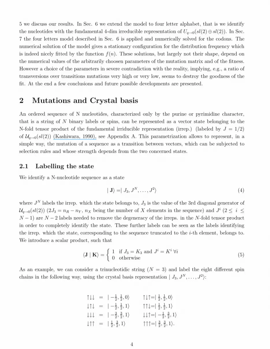
2 Mutations and Crystal basis

An ordered sequence of N nucleotides, characterized only by the purine or pyrimidine character,

that is a string of N binary labels or spins, can be represented as a vector state belonging to the

N-fold tensor product of the fundamental irriducible representation (irrep.) (labeled by J = 1/2)

of Uq→0(sl(2)) (Kashiwara, 1990), see Appendix A. This parametrization allows to represent, in a

simple way, the mutation of a sequence as a transition between vectors, which can be subjected to

selection rules and whose strength depends from the two concerned states.

2.1 Labelling the state

We identify a N-nucleotide sequence as a state

| J〉 =| J3, JN , . . . , J2〉 (4)

where JN labels the irrep. which the state belongs to, J3 is the value of the 3rd diagonal generator of

Uq→0(sl(2)) (2J3 = nR − nY , nX being the number of X elements in the sequence) and J i (2 ≤ i ≤

N − 1) are N − 2 labels needed to remove the degeneracy of the irreps. in the N -fold tensor product

in order to completely identify the state. These further labels can be seen as the labels identifying

the irrep. which the state, corresponding to the sequence truncated to the i-th element, belongs to.

We introduce a scalar product, such that

〈J | K〉 =

{1 if J3 = K3 and J i = Ki ∀i0 otherwise

(5)

As an example, we can consider a trinucleotidic string (N = 3) and label the eight different spin

chains in the following way, using the crystal basis representation | J3, JN , . . . , J2〉:

↑↓↓ = | −12, 1

2, 0〉 ↑↓↑=| 1

2, 1

2, 0〉

↓↑↓ = | −12, 1

2, 1〉 ↑↑↓=| 1

2, 1

2, 1〉

↓↓↓ = | −32, 3

2, 1〉 ↓↓↑=| −1

2, 3

2, 1〉

↓↑↑ = | 12, 3

2, 1〉 ↑↑↑=| 3

2, 3

2, 1〉.

4

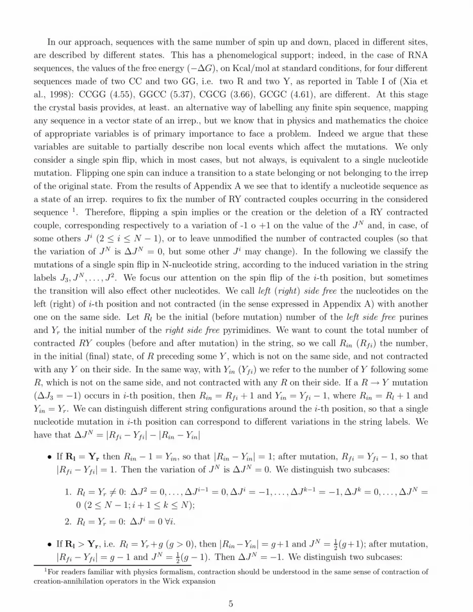
In our approach, sequences with the same number of spin up and down, placed in different sites,

are described by different states. This has a phenomelogical support; indeed, in the case of RNA

sequences, the values of the free energy (−∆G), on Kcal/mol at standard conditions, for four different

sequences made of two CC and two GG, i.e. two R and two Y, as reported in Table I of (Xia et

al., 1998): CCGG (4.55), GGCC (5.37), CGCG (3.66), GCGC (4.61), are different. At this stage

the crystal basis provides, at least. an alternative way of labelling any finite spin sequence, mapping

any sequence in a vector state of an irrep., but we know that in physics and mathematics the choice

of appropriate variables is of primary importance to face a problem. Indeed we argue that these

variables are suitable to partially describe non local events which affect the mutations. We only

consider a single spin flip, which in most cases, but not always, is equivalent to a single nucleotide

mutation. Flipping one spin can induce a transition to a state belonging or not belonging to the irrep

of the original state. From the results of Appendix A we see that to identify a nucleotide sequence as

a state of an irrep. requires to fix the number of RY contracted couples occurring in the considered

sequence 1. Therefore, flipping a spin implies or the creation or the deletion of a RY contracted

couple, corresponding respectively to a variation of -1 o +1 on the value of the JN and, in case, of

some others J i (2 ≤ i ≤ N − 1), or to leave unmodified the number of contracted couples (so that

the variation of JN is ∆JN = 0, but some other J i may change). In the following we classify the

mutations of a single spin flip in N-nucleotide string, according to the induced variation in the string

labels J3, JN , . . . , J2. We focus our attention on the spin flip of the i-th position, but sometimes

the transition will also effect other nucleotides. We call left (right) side free the nucleotides on the

left (right) of i-th position and not contracted (in the sense expressed in Appendix A) with another

one on the same side. Let Rl be the initial (before mutation) number of the left side free purines

and Yr the initial number of the right side free pyrimidines. We want to count the total number of

contracted RY couples (before and after mutation) in the string, so we call Rin (Rfi) the number,

in the initial (final) state, of R preceding some Y , which is not on the same side, and not contracted

with any Y on their side. In the same way, with Yin (Yfi) we refer to the number of Y following some

R, which is not on the same side, and not contracted with any R on their side. If a R → Y mutation

(∆J3 = −1) occurs in i-th position, then Rin = Rfi + 1 and Yin = Yfi − 1, where Rin = Rl + 1 and

Yin = Yr. We can distinguish different string configurations around the i-th position, so that a single

nucleotide mutation in i-th position can correspond to different variations in the string labels. We

have that ∆JN = |Rfi − Yfi| − |Rin − Yin|

• If Rl = Yr then Rin − 1 = Yin, so that |Rin − Yin| = 1; after mutation, Rfi = Yfi − 1, so that

|Rfi − Yfi| = 1. Then the variation of JN is ∆JN = 0. We distinguish two subcases:

1. Rl = Yr 6= 0: ∆J2 = 0, . . . ,∆J i−1 = 0,∆J i = −1, . . . ,∆Jk−1 = −1,∆Jk = 0, . . . ,∆JN =

0 (2 ≤ N − 1; i+ 1 ≤ k ≤ N);

2. Rl = Yr = 0: ∆J i = 0 ∀i.

• If Rl > Yr, i.e. Rl = Yr +g (g > 0), then |Rin−Yin| = g+1 and JN = 12(g+1); after mutation,

|Rfi − Yfi| = g − 1 and JN = 12(g − 1). Then ∆JN = −1. We distinguish two subcases:

1For readers familiar with physics formalism, contraction should be understood in the same sense of contraction ofcreation-annihilation operators in the Wick expansion

5

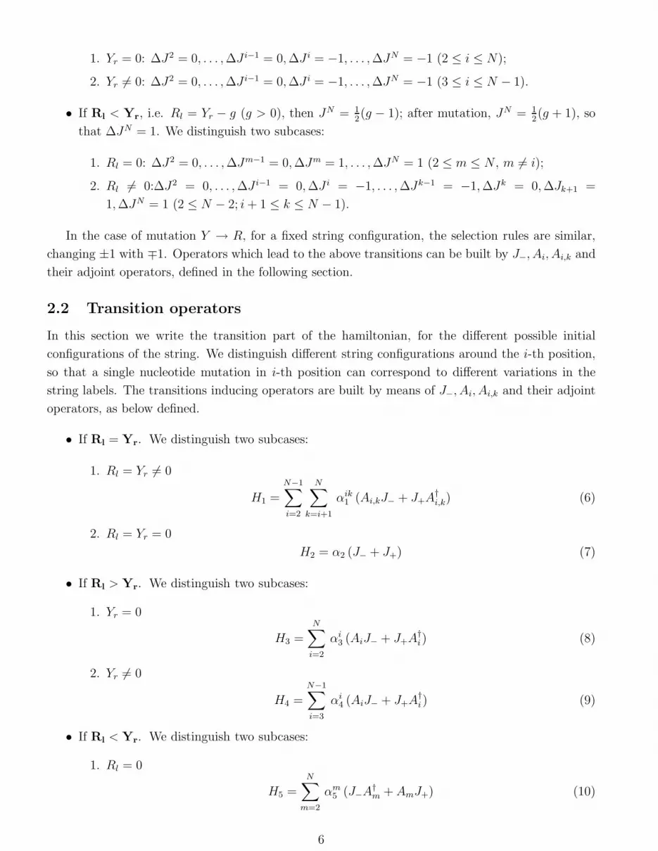
1. Yr = 0: ∆J2 = 0, . . . ,∆J i−1 = 0,∆J i = −1, . . . ,∆JN = −1 (2 ≤ i ≤ N);

2. Yr 6= 0: ∆J2 = 0, . . . ,∆J i−1 = 0,∆J i = −1, . . . ,∆JN = −1 (3 ≤ i ≤ N − 1).

• If Rl < Yr, i.e. Rl = Yr − g (g > 0), then JN = 12(g − 1); after mutation, JN = 1

2(g + 1), so

that ∆JN = 1. We distinguish two subcases:

1. Rl = 0: ∆J2 = 0, . . . ,∆Jm−1 = 0,∆Jm = 1, . . . ,∆JN = 1 (2 ≤ m ≤ N , m 6= i);

2. Rl 6= 0:∆J2 = 0, . . . ,∆J i−1 = 0,∆J i = −1, . . . ,∆Jk−1 = −1,∆Jk = 0,∆Jk+1 =

1,∆JN = 1 (2 ≤ N − 2; i+ 1 ≤ k ≤ N − 1).

In the case of mutation Y → R, for a fixed string configuration, the selection rules are similar,

changing ±1 with ∓1. Operators which lead to the above transitions can be built by J−, Ai, Ai,k and

their adjoint operators, defined in the following section.

2.2 Transition operators

In this section we write the transition part of the hamiltonian, for the different possible initial

configurations of the string. We distinguish different string configurations around the i-th position,

so that a single nucleotide mutation in i-th position can correspond to different variations in the

string labels. The transitions inducing operators are built by means of J−, Ai, Ai,k and their adjoint

operators, as below defined.

• If Rl = Yr. We distinguish two subcases:

1. Rl = Yr 6= 0

H1 =

N−1∑

i=2

N∑

k=i+1

αik1 (Ai,kJ− + J+A

†i,k) (6)

2. Rl = Yr = 0

H2 = α2 (J− + J+) (7)

• If Rl > Yr. We distinguish two subcases:

1. Yr = 0

H3 =

N∑

i=2

αi3 (AiJ− + J+A

†i) (8)

2. Yr 6= 0

H4 =

N−1∑

i=3

αi4 (AiJ− + J+A

†i ) (9)

• If Rl < Yr. We distinguish two subcases:

1. Rl = 0

H5 =N∑

m=2

αm5 (J−A

†m + AmJ+) (10)

6

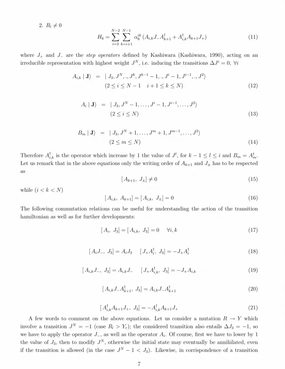
2. Rl 6= 0

H6 =

N−2∑

i=2

N−1∑

k=i+1

αik6 (Ai,kJ−A

†k+1 + A†

i,kAk+1J+) (11)

where J+ and J− are the step operators defined by Kashiwara (Kashiwara, 1990), acting on an

irreducible representation with highest weight JN , i.e. inducing the transitions ∆J i = 0, ∀i

Ai,k | J〉 = | J3, JN , ., Jk, Jk−1 − 1, ., J i − 1, J i−1, ., J2〉

(2 ≤ i ≤ N − 1 i+ 1 ≤ k ≤ N) (12)

Ai | J〉 = | J3, JN − 1, . . . , J i − 1, J i−1, . . . , J2〉

(2 ≤ i ≤ N) (13)

Bm | J〉 = | J3, JN + 1, . . . , Jm + 1, Jm−1, . . . , J2〉

(2 ≤ m ≤ N) (14)

Therefore A†i,k is the operator which increase by 1 the value of J l, for k − 1 ≤ l ≤ i and Bm = A†

m.

Let us remark that in the above equations only the writing order of Ak+1 and J± has to be respected

as

[Ak+1, J±] 6= 0 (15)

while (i < k < N)

[Ai,k, Ak+1] = [Ai,k, J±] = 0 (16)

The following commutation relations can be useful for understanding the action of the transition

hamiltonian as well as for further developments:

[Ai, J3] = [Ai,k, J3] = 0 ∀i, k (17)

[AiJ−, J3] = AiJ3 [ J+A†i , J3] = −J+A

†i (18)

[Ai,kJ−, J3] = Ai,kJ− [ J+A†i,k, J3] = −J+Ai,k (19)

[Ai,kJ−A†k+1, J3] = Ai,kJ−A

†k+1 (20)

[A†i,kAk+1J+, J3] = −A†

i,kAk+1J+ (21)

A few words to comment on the above equations. Let us consider a mutation R → Y which

involve a transition JN = −1 (case Rl > Yr); the considered transition also entails ∆J3 = −1, so

we have to apply the operator J−, as well as the operator Ai. Of course, first we have to lower by 1

the value of J3, then to modify JN , otherwise the initial state may eventually be annihilated, even

if the transition is allowed (in the case JN − 1 < J3). Likewise, in corrispondence of a transition

7

Y → R (∆J3 = +1), first the change JN → JN + 1 has to be maked, then J3 → J3 + 1. To write a

self-adjoint operator, we have to add to the operator, which gives rise to the transition Y → R, the

one which leads to R → Y , leaving the rest of the string unmodified, that is

AiJ− + J+A†i (22)

This operator leads to the mutation Y → R or R → Y for a nucleotide in i-th position, in a string

with Rl > Yr. If the mutation R → Y rises the value of JN , first JN has to be modified, then J3;

with the aim to write a self adjoint operator, we write

J−A†m + AmJ+ (23)

The above operator gives rise to mutations R → Y and Y → R for a nucleotide in i-th position,

preceding the m-th one, in the case Rl = 0, Yr 6= 0. Let us remark that eq.(9) is included in eq.(8), if

the coupling constants αi4 are assumed equal to αi

3; in eq.(11), only the writing order for Ak+1 (and

its adjoint) and J± has to be respected. Let us also note that when ∆JN = 0 there is no need to

order the operators.

3 The quantum spin model

Assuming now that the coupling constants do not depend on i, k,m, we can write the transition

hamiltonian HI as

HI = µ1(H3 +H5) + µ2H1 + µ3H2 + µ4H6 (24)

The total hamiltonian of the model will be written as

H = H0 + HI (25)

where H0 is the diagonal part in the choosen basis and, in the following, is assumed to be H0 = µ0 J3.

We let the fenomenology suggests us the scale of the values of the coupling constants of HI . We want

to write an interaction term which makes the mutation in alternating purinic/pyrimidinic tracts less

likely than in polypurinic or polypyrimidinic ones. We mean as a single nucleotide mutation in a

polypurinic (polypyrimidinic) tract, a mutation inside a string with all nucleotides R (Y ), i.e. a

highest (lowest) weight state. Such a transition corresponds to the selection rules ∆JN = −1,∆J3 =

±1, i.e. a transition generated by the action of H3 and H5. In the interaction term HI , we give them

a coupling constant smaller than the others terms. We introduce, for ∆J3 = ±1 , only four different

mutation parameters µi (i = 1, 2, 3, 4), with µ1 < µk, k > 1.

1. µ1 for mutations which change the irrep., ∆JN = ±1, and include the spin flip inside an

highest or lowest weight vector;

2. µ2 for mutations which do not change the irrep., ∆JN = 0, but modifies other values of Jk,

∆Jk = ±1;

3. µ3 for mutations which do not change the irrep., ∆JN = 0, neither the other values of Jk,

∆Jk = 0, (2 ≤ k ≤ N − 1);

8

4. µ4 for mutations which change the irrep., ∆JN = ±1, but only in a string with 0 6= Rl < Yr.

We do not introduce another parameter, for mutations generated by H4, i.e. i-th nucleotide mutation

in a string with Rl > Yr 6= 0, not to distinguish, in a polypurinic string, between a mutation in 2-th

position and another one inside the string. Let us emphasize once more that the proposed model

takes into account, at least partially, the effect on the transition in the i-th site of the distribution

of all the spins. Presently we consider only the part of the interaction hamiltonian HI , which

generates transitions corresponding to one spin flip write, but, in analogous way, we could write

more complicated transition operators. Let us illustrate, in a simple example, the difference between

this scheme and the standard one, based on the hypotesis of transition probability between chains,

only depending by their Hamming distance. Let us consider the following string RRRRR. By a

single flip spin the string goes in one of the following configurations:

1) Y RRRR 2) RY RRR 3) RRY RR 4) RRRY R 5) RRRRY (26)

In the models based on the Hamming distance, all the transitions are equally probable, as the final

strings are all at the same distance from the original one. In the present scheme the 1-rst transition

is ruled by the value of µ3, the transition 2-5 are ruled by µ1 .

Let us stress that our scheme is not equivalent to an Ising model with the transition strength

depending on the position. To illustrate the difference with a few examples let us consider the

transitions RY Y RR → RY Y Y R , RY Y RY → RY Y Y Y , both with a flip in the fourth position,

the first one ruled by µ2, the second one by µ1. Mutations in different points can be ruled by the

same coupling constant: RY Y RR → RY Y Y R , RY RRY → RY Y RY with a flip, respectively,

in the 4th and 3rd position ruled by µ2. As already said, the main motivation for introducing

this quantum model is that it provides the formal and conceptual language to write the transitions,

ensuring in the same time, due to the unitary character of the evolution operator, the conservation

of the probability. We shall briefly describe in Sec. 6 the outcome of this model, see (Minichini

and Sciarrino 2004a) for more details, which has only been reported to make, hopefully, more clear

the structure of the classical model of the next section. Let us point out that there are very strong

drawback in trying to further pursue the study of the quantum model, for example superposed states,

that is linear combinations of sequences, do exist in such models, while only the different sequences

have a biophysical interpretation.

4 The classical model

In the previous section we have introduced mutation inducing operators based on the change of the

global labels J i. Using these results as a guide we write a kinetic equations systems in which the non

vanishing mutation matrix entries depend on the labels of the connected sequences. We are interested

in finding the stationary or equilibrium configuration of the 2N different possible sequence. Writing

pJ(t) the probability distribution at time t of the sequence identified by the vector | J〉, a decoupled

version of selection mutation equation, (see (Hofbauer and Sigmund, 1988) for an exhaustive review),

for a haploid organism, can be written as

d

dtpJ(t) = pJ(t)

(RJ −

∑

K

RK pK(t)

)+∑

K

MJ,K pK(t) (27)

9

where RK is the Malthusian fitness of the sequence corresponding to the vector | K〉 and MJ,K are

the entries of a mutation matrix M which satisfies

MJ,J = −∑

K 6=J

MJ,K (28)

The equation (27) is reduced to

d

dtxJ(t) =

∑

K

(H +M)J,K xK(t) (29)

where

xJ(t) = pJ(t) exp

(∑

K

RK

∫ t

0

pK(τ) dτ

)(30)

and H is a diagonal matrix, with fitness as entries (RK = HK,K). In our model the mutation matrix

is written as the sum of the partial mutation matrices Mi which are obtained by the interaction

hamiltonians Hi replacing the adjoint operators by the transposed (denoted by an upper labe T ).

Assuming now that the coupling constants do not depend on i, k,m, we can write the mutation

matrix M as (Minichini and Sciarrino, 2004b)

M = µ1(M3 +M5) + µ2M1 + µ3M2 + µ4M6 +MD (31)

where MD is the diagonal part of the mutation matrix defined by eq.(28). The hierarchy of the values

of the coupling constants is fixed as in the previous section.

5 Results

The evolution equation of the model for the probabilities will be written in terms of the matrix

H = H + M + λ1, where the fitness can be H = J3 (purely additive fitness) and λ is choosen in

such a way to guarantee H is positive. Being H + M irreducible, the composition of equilibrium

population is given by

pJ =xJ∑KxK

(32)

where xJ is the Perron-Frobenius eigenvector, see, e.g. (Encyclopedic Dictionary of Mathematics,

1960) of H . In (Minichini and Sciarrino, 2004b) the numerical solutions of the model have been

reported, with a suitable choice of the value of the parameters, for N = 3,4,6. Before discussing these

results, we point out explicitly the main features of our model. M describes an interaction on the i-th

spin neither depending on the position nor on the nature of the closest neighbours, but which takes

into account, at least partially, the effects, on the transition in the i-th site, of the distribution of all

the spins, that is non local effects. Indeed it depends on the “ordered” spin orientation surplus on

the left and on the right of the i-th position. Should it not depend on the order, it may be considered

as a mean-field like effect. Moreover ∆J3 = ±1 transitions are allowed, which, e.g. for N = 4, can

be considered or as the flip of a spin combined with an exchange of the two, oppositely oriented,

previous or following spins or as the collective flip of particular three spin systems, containing a two

spin system with opposite spin orientations (see example below). Biologically, the transition depends

10

in some way on the ”ordered” purine surplus on the left and on the right of the mutant position.

Let us briefly comment on the physical-biological meaning of the “ordered” spin sequence. Our aim

is to study finite oligonucleotide sequence in which a beginning and an end are defined. This implies

we can neither make a thermodynamic limit on N nor define periodic conditions on the spin chain.

So we have to take into account the “edge” or “boundary” conditions on the finite sequence. An

analogous problem appears in determing thermodynamic properties of short oligomers and, in this

framework, in (Goldstein and Benight, 1992) the concept of fictitious nucleotide pairs E and E’ has

been introduced, in order to mimick the edge effects. The ordered couple of RY takes into account in

some way the different interactions of R and Y with the edges. For example, the transition matrix,

on the above basis (for N = 3) is the following one, up to a multiplicative dimensional factor µ0

M =

x δ 0 γ ǫ 0 ǫ 0δ x 0 0 0 ǫ 0 ǫ0 0 x δ ǫ 0 ǫ 0γ 0 δ x 0 ǫ 0 ǫǫ 0 ǫ 0 x δ 0 00 ǫ 0 ǫ δ x δ 0ǫ 0 ǫ 0 0 δ x δ0 ǫ 0 ǫ 0 0 δ x

(33)

where the diagonal entries x, not explicitly written, are given by eq.(28). Note that the above matrix

depends only on three coupling constants due to the very short length of the chain. For N ≥ 4

the 4th coupling constant (denoted in the following by η) will appear. Let us emphasize that the

mutation matrix M (33) does not only connect states at unitary Hamming distance. As an example,

we write explicitly the transitions from | 12, 1

2, 0〉 (↑↓↑) and from | −1

2, 1

2, 0〉 (↑↓↓)

↑↓↑−→

↑↑↑↓↓↑↑↓↓

↑↓↓−→

↓↑↑↓↓↓↑↑↓↑↓↑

The first transition of the second example can be regarded as a spin-flip of the three spins. Let we

explicitly write, for N = 3, the mutation matrix, which allows transitions only between chains at

Hamming distance equal to one, with coupling constant α.

HHamm =

y α 0 α α 0 0 0α y 0 0 0 α 0 α0 0 y α α 0 α 0α 0 α y 0 0 0 αα 0 α 0 y α 0 00 α 0 0 α y α 00 0 α 0 0 α y α0 α 0 α 0 0 α y

(34)

where the diagonal entries, not explicitly written, are given by eq.(28). Note that, even if we put in

eq.(33) all the constant equal to α (δ = γ = ε = α), we do not get the Hamming hamiltonian (34).

If we order (in a decreasing way) the equilibrium probabilities, we obtain, using the mutation matrix

with Hamming distance, a rank ordered distribution of transition probability like that in fig.1 for

11

N = 4. Its shape does not depend on the value of α. The rank-ordered distribution of the probabilities

shows a plateaux structure: every plateaux contains spin sequences at the same Hamming distance

from the sequence with the highest value of the fitness. Using the mutation matrix (33), the rank

ordered probabilities distribution does not show a plateaux structure, but its shape is well fitted by

a Yule distribution (fig.2), like the observed frequency distribution of oligonucleotidic in the strings

of nucleic acids (Martindale and Konopka, 1996). Let us observe that we obtain a Yule distribution

(and not a plateaux structure) even if all parameters in (33) are tuned at the same value, which

means that the distribution is the outcome of the model and not of the choice of the values of the

coupling constants. Analogous resultes are obtained for N = 6 (fig.3). Let us point out that:

i) our model is not equivalent to a model where the intensity depends on the site undergoing the

transition, or from the nature of the closest neighbours or the number of the R and Y labels of the

sequence; indeed essentially the intensity depends on distribution in the sequence of the R and Y ;

ii) the ranked distribution of the probabilities follows a Yule distribution law, but as the value of

the parameter b is close to the unity, the distribution is equally well fitted by a Zipf law (Zipf, 1949)

(f = a nk), in agreement with the remark of (Martindale and Konopka, 1996).

Let us also briefly recall the outcomes of the genetically inspired quantum spin model presented

in Sec. 3. We can study the time evolution of an initial state, representing a given spin chain,

and evaluate the probability of transition in another one, if H is the hamiltonian which generates

the dynamics of the system. The matrix form of H , on the above basis for a fixed initial state,

is obtained (for N = 3), by replacing in eq.(33) the diagonal terms by the eigenvalues of J3, i.e.

by, respectively, (-1,1,-1,1,-3,-1,1,3) (up a multiplicative factore 1/2). Analogously we can study the

dynamics of an ordered quantum spin chain, with an interaction Hamiltonian, leading to transitions

with the same probability between nucleotide strings at unit Hamming distance, whose matrix, for

N = 3, is obtained by eq.(34) by replacing the diagonal terms with the eigenvalues of J3. In order to

evaluate the probabilities of transition, we cannot analytically study the time evolution of an initial

state, representing a fixed spin sequence, as ruled by eq.(33) with the change of the diagonal terms,

but we can find a numerical solution. The transition probability between two states, belonging to

the crystal basis, exhibits the quantum mechanically typical oscillating behaviour as a function of

the time. We define a time-averaged transition probability (initial state (i) −→ final state (f))

< pif >=1

T

∫ T

0

pif(t) dt (35)

where the value of T will be numerically fixed to a value, such that the r.h.s. of eq.(35) becomes stable.

If we order (in a decreasing way) the average transition probability from an initial state to every

other chain, if (34) is the hamiltonian, we obtain a rank ordered distribution of transition probability

like that in fig.1. Its shape does not depend by the choice of initial state or by the coupling constant

α value. We always get the same structure, for models with transition probability only depending

on Hamming distances. So the rank-ordered distribution of the average transition probability shows

a plateaux structure: every step contains spin chains at the same Hamming distance from the initial

one. In the case of the model which we propose here, i.e. the hamiltonian in (33), which we call

crystal basis model, the distribution of rank ordered average transition probability does not show a

plateaux structure, but its shape is well fitted by a Yule distribution like that in fig.2. Also in the

12

quantum model, we obtain a Yule distribution (and not a plateaux structure) even if all parameters

in (33) are tuned at the same value. In this case, the state, labelled by 1 in the plots, is the initial

one. The ranked distribution of the probabilities, not averaged in time, computed for several values

of the time, also follows generally a Yule distribution law. Moreover we still remark that, for the

highest value of N , the distribution is equally well fitted by a Zipf law, i.e. b = 1 in eq.(1), but not

for the lowest values of N , in agreement with the remark of (Martindale and Konopka, 1996.

6 The four letter model

In order to label a sequence of N nucleotides, taking into account that they belong to the four letter

set {C,T/U,G,A}, we assign the 4 nucleotides to the 4-dim irreducible fundamental representation

(irreps.) (1/2, 1/2) of Uq→0(sl(2) ⊕ sl(2)) (Frappat, Sciarrino and Sorba, 1998) with the following

assignment for the values of the third component of ~J for the two sl(2) which in the following will

be denoted as slH(2) and slV (2) :

C ≡ (+12,+1

2) T/U ≡ (−1

2,+1

2) G ≡ (+1

2,−1

2) A ≡ (−1

2,−1

2) (36)

It follows that an ordered sequence of N nucleotides can be represented as a vector belonging to

the N-fold tensor product of the fundamental irriducible representation of Uq→0(sl(2) ⊕ sl(2)), in a

straightforward generalization of the approach followe in Sec.2 for Uq→0(sl(2)). In the following we

use the symbols X for C,G and Z for U,A. In the formalism of Uq→0(sl(2) ⊕ sl(2)) all the previous

results have to be understood to refer to slV (2). Now we identify a N-nucleotide sequence as a state

| JHJV 〉 =| J3,H , J3,V ; JNH , J

NV ; . . . ; J2

H , J2V 〉 (37)

where JNm (m = H, V ) labels the irrep. which the state belongs to, J3,m is the value of the 3rd

diagonal generator of Uq→0(slm(2)) (2J3,H = nX − nZ , 2J3,V = nR − nY ) and J im (2 ≤ i ≤ N − 1)

are 2(N − 2) labels needed to completely identify the state. As an example, the trinucleotidic string

CGA is labeled by

| CGA〉 =|(

12

)H,−(

12

)V

;(

12

)H,(

12

)V

; (1)H (1)V 〉 (38)

The previously introduced scalar product is straightforwardly generalized. In the present paper,

we only consider a single spin flip in H or V spin or in both H and V, which in most cases, but

not always, is equivalent to a single nucleotide mutation. Obviously a H spin flip (V and H,V flip)

corresponds, respectively, to a biological transition (transversion). Flipping one spin can induce a

transition to a state belonging or not belonging to the irrep. of the original state. From an immediate

generalisation of the results of Appendix A, we need, to identify a nucleotide sequence as a state of

an irrep., to fix the number of RY and XZ contracted couples occurring in the considered sequence.

Therefore flipping a spin implies or the creation or the deletion of a RY or XZ or both contracted

couple, corresponding, respectively, to a variation of -1 o +1 on the value of the JNV , JN

H or both

and, possibly, of some others J im (2 ≤ i ≤ N − 1), or to leave unmodified the number of contracted

couples (so that ∆JNm = 0, but some other J i

m are modified). We focus our attention on the spins

flip of the i-th position and we go on in a completely analogous way as in Sec. 2, but taking into

13

account the two couples RY and XZ. Assuming, as previously, that the coupling constants do not

depend on i, k,m, we write the mutation matrix M as

M = MH +MV

= µ1(M3,H +M5,H) + µ2M1,H + µ3M2,H + µ4M6,H

+ λ1(M3,V +M5,V ) + λ2M1,V + λ3M2,V + λ4M6,V +MD (39)

whereMD is the diagonal part of the mutation matrix defined by eq.(28), andMk,m (k = 1, 2, 3, 5, 6;m =

H, V ) are the off-diagonal mutation matrices defined by the following operators, where we have omit-

ted to explicitly write the coupling constants

H1,m = Ai,k;mJ−,m + J+,mA†i,k;m (40)

H2,m = J−,m + J+,m (41)

H3,m = Ai;mJ−,m + J+,mA†i;m (42)

H4,m = Ai;mJ−,m + J+,mA†i;m (43)

H5,m = J−,mA†m;m + Am;mJ+,m (44)

H6,m = Ai,k;mJ−,mA†k+1;m + A†

i,k;mAk+1;mJ+,m) (45)

Note that in eq.(39) we have not introduced a coupling term between the two sl(2), i.e. a mutation

matrix of the type MH,V ∝ J+,HJ+,V or MH,V ∝ J−,HJ−,V . In order to fit the phenomenological

observation that the transitions occur more frequently than the transversions, we have to fix the

coupling constants λ of the order of 1/2 − 1/3 of the coupling constants µ. Let us remark that,

with the chosen mutation matrix eq.(39), a single spin mutation does not correspond necessarily to

a H-spin or V-spin flip. Indeed the mutations C ↔ A amd T ↔ G imply a flip of both the H and V

spins, therefore these mutations should be depressed.

7 The rank ordered distribution of codons

In (Frappat, Sciarrino and Sorba, 1998) a mathematical model, called crystal basis model, for the

genetic code has been proposed where from the assignment eq.(36) of the four nucleotides to the

4-dim fundamental (12, 1

2) irreducible representation of the quantum group Uq→0(sl(2) ⊕ sl(2)), the

codons (3-nucleotide sequence) appear as composite state in the3-fold tensor product of (12, 1

2). From

the general formalism of the previous section, a codon is identified as a state

| JH〉⊗ | JV 〉 ≡| JHJV 〉 =| J3,H , J3,V ; J3HJ

3V ; J2

H , J2V 〉 (46)

14

For example we have, see (Frappat, Sciarrino and Sorba, 2001) for a list of all the states:

| CGA〉 =|(

12

)H,−(

12

)V

;(

12

)H,(

12

)V

; (1)H (1)V 〉

The mutation matrix eq.(39) now becomes

M =∑

m=H,V

∑

i=2,3

µ1,m[(Ai,mJ−,m + J+,mATi,m)

+ (J−,mATi,m + Ai,mJ+,m)] + µ2,m (J−,m + J+,m)

+ µ3,m(BmJ−,m + J+,mBTm) +MD,m

where

Bm | J〉 = | J3,m, J3m, J

2m − 1〉 (47)

Ai,m | J〉 = | J3,m, J3m − 1, . . . J i

m − 1, . . .〉 (2 ≤ i ≤ 3) (48)

and MD is the diagonal part of the mutation matrix. We are interested in finding the stationary

configuration solution of the eq.(27) for the 64 different possible sequences. We choose the following

form for the (purely additive) fitness H = J3,H + J3,V + λ1, λ > 0 ensuring H + M to be positive.

Below we report several representative figures in which the obtained numerical solutions are fitted

with a function given by eq.(2) (we omit the hat on the parameters). In figg.4-5, with a suitable choice

of the values of the parameters, our results are well fitted. In fig.6 we report another solution where

the ratio, denoted by (H/V ), between the mutation intensity between transitions and transversions,

is chosen larger than one, but the value of the coupling constants do not satisfy the hierarchy

µ1,H < µ2,H , µ3,H , which is less well fitted. In fig.7 we report another solution with a unrealistic

choice of the values of the parameters of the ratio (H/V ) ((H/V ) ≈ 10), which is, indeed, badly fitted

by a function given by eq.(2). Finally in fig.8 we report another solution, also badly fitted, where

(H/V ) ≈ 10−1. This last result is a consequence of the fact that we have chosen a fitness symmetric

for the exchange H ↔ V . Therefore the exchange of the values of the coupling constants between MH

and MV gives the same shape of the distribution. Of course the rank of the same codon is, in general,

different in the two cases. Summarizing, we can state that the numerical solutions of our model, for

arbitrary choice of the values of the coupling constants, are rather well fitted by a function of the type

given in eq.(2), with a suitabe choice of the parameters, but that a non realistic choice of the values

of the coupling constants, e.g. a ratio of transversion/transition mutation very high or very low,

seems to destroy the goodness of the fit. Moreover, it is quite surprising to remark that the values

of the parameters in the function eq.(2), which fits our numerical solutions, are of the same order

of magnitude of the parameters (depending on the total GC content) found in (Frappat, Minichini,

Sciarrino and Sorba, 2003) to best fit the observed rank ordered distribution. In the present paper,

the values of α and η are found to be slightly larger than the ones computed in (Frappat, Minichini,

Sciarrino and Sorba, 2003). Let us stress once more that a mutation matrix M , with non diagonal

non vanishing entries connecting only codons with Hamming distance equal to one, is unable to

reproduce the observed rank ordered distribution as it induces mutation between classes of codons

at the same Hamming distance. We have considered separately the finess and mutation matrix for

the horizontal and vertical labels of the codons. As, a priori, one can consider also a coupling term

15

between the two parts, our simplified treatment has to be considered as a first step in the way of

constructing a realistic model. We have also performed a preliminary analysis with a a value, ρH , of

the horizontal fitness different from the value, ρV of the vertical one. It appears that the outcome

depends on the ratio ρH/ρV as well as on the ratio between the values of the ρ and the value of the

transition coupling constant µ (beside the discussed dependence on the ratio of µH/µV and on the

hierarchy of the values of the differents µH and µV ). So we believe that a better understanding of the

form of the fitness and of the hierarchy of the values of the mutation parameters, as well as on the

reliability of a model which explains the rank ordered distribution of the codons as a consequence of

the mutation-selection of 64 triplets, is necessary before further pursuing the numerical analysis .

8 Conclusions

We have proposed a model not analytically soluble, but which admits an easy numerical solution for

short spin chains. Let us emphasize that the main purpose of the proposed scheme is to take into

account, at least partially, the effects of the neighbours in the mutation. We point out, once more,

that our model is not equivalent to a model where the intensity depends on the site undergoing the

transition, or on the nature of the closest neighbours or on the number of the R and Y labels of the

sequence; indeed essentially the intensity depends on the distribution in the sequence of the R and

Y . We find that the numerically computed stationary distribution for short oligonucleotides to follow

a Yule o Zipf law, in agreement with the observed distribution. We are far from claiming, for several

obious reasons, that our simple model is the only model able to explain the observed oligonucleotide

distribution, but that the standard approach using the Hamming distance does not provide such a

solution. One may correctly argue that the comparison between the Hamming model, depending on

only one parameter and taking into account only one site spin flip, with our model, which depends

on four parameters and takes into account spin flip of more than one site, is not meaningful. So

we have computed the stationary distribution with a mutation matrix not vanishing for Hamming

distance larger than one and allowing the same number of mutations as our model. The result

reported in fig.9 shows that the plateaux structure is always the dominant feature. Let us comment

on the non point mutations which naturally are present in our model. In literature there is an

increasing number of papers that, on the basis of more accurate data, question both the assumptions

that mutations occur as single nucleotide and as independent point event. In a quite recent paper

(Whelan and Goldman, 2004) have presented a model allowing for single-nucleotide, doublet and

triplet mutation, finding that the model provides statistically significant improvements in fits with

protein coding sequences. We note that the triplet mutations, for which there is no known inducing

mechanism, but which can possibly be explained by large scale event, called sequence inversion in

(Whelan and Goldman, 2004), are indeed the kind of mutations, above discussed, that our model

naturally describes. Doublet mutations do not appear, due to the assumed spin flip equal ±1, but

on one side some of these mutations are hidden by the binary approximation, and on the other side

the parameter ruling such mutations, as computed in (Whelan and Goldman, 2004), is lower than

the one ruling the triplet mutation. In conclusion the Hamming distance does not seem a suitable

measure of the distance in the space of the biological sequences, the crystal basis, on the contrary,

seems a better candidate to parametrize the elements of such space. Our model makes use of this

16

parametrisation, allows to modelise some non point mutations and exhibits intriguing and interesting

features, hinting in the right direction, worthwhile to be further investigated. In the present simple

version, the model depends only on 4 (8) parameters in the two letter (resp. four letter) alphabet

for any N, which are, very likely, not enough to describe sequences longer that the considered ones.

However the model is rather flexible: as shown in the case of the codons, it is easily generalised to

the four letter alphabet; besides the obvious introduction of more coupling constants, it allows, e.g.,

to analyse part of the sequences containing hot spots in the mutation, to take into account doublet

mutations (indeed the operator eq.(12) or ATi,i+1 describes a doublet spin flip at position i,i+1).

Although the very short chain, which we were interested in, can be studied numerically without any

use of the crystal basis, we propose a general algorithm, which can be applied to chains of arbitrary

length and which can be easily implemented in computers. It is worthwhile to remark that we are

trying to compare theoretical results, deriving from simple models, to really observed data, coming

from the extremely complex biological world. In this context the crystal basis provides a compact

and useful notation to describe the “kinematical” variables which are changed by the dynamics.

The generalisation of our approach to the a four letters alphabet, which is easily done replacing

Uq(sl(2)) by Uq(sl(2) ⊕ sl(2)), has been presented and applied to the study of the mutations of the

codons. As expected, calculations are more complicated and only a few results in the simple case

of the triplets are given. In this framework, further investigation deserve attention, in particular to

study oligonucleotide distribution in the four letters alphabet and mutations in long sequences. In

conclusion we point out that:

• the crystal basis provides an alternative way of labelling nucleotide sequences, in particular

codons or genes, mapping any finite ordered nucleotide sequence in a vector state of an irrep..

We point out that the choice of the limit q → 0 (crystal basis) is essential for the above

identification as, only in this limit, due to Kashiwara theorem (Kashiwara, 1990), the composite

states are pure states.

• the mutation matrix M in our model describes an interaction on the i-th nucleotide depending

on the input-output sequences and, in the flip of one spin (or double spin), inherently takes

into account non local effects. So the crystal basis variables are suitable to partially describe

non local events which affect the mutations.

• models based on the crystal basis seem, in the light of the obtained results, better candidates

than models based on Hamming distance to describe mutations.

As final remark, this article should be seen as a first, simplified attempt to build models, more

realistic than the ones based on the Hamming distance, to describe the effects of the mutation-

selection on the observed distribution of oligonucleotides.

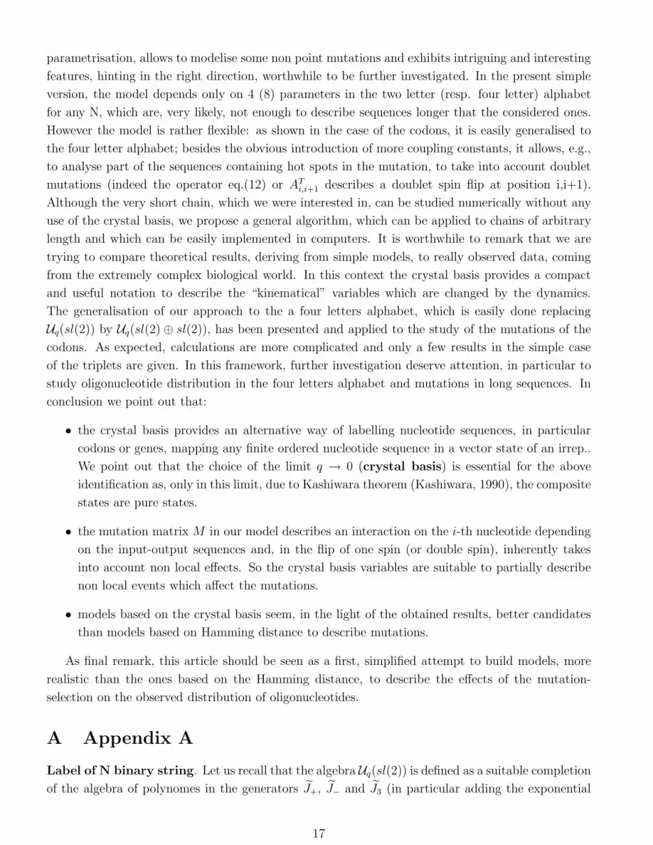
A Appendix A

Label of N binary string. Let us recall that the algebra Uq(sl(2)) is defined as a suitable completion

of the algebra of polynomes in the generators J+, J− and J3 (in particular adding the exponential

17

series), subject to the following commutation relations:

[J+, J−] = [2J3]q

[J3, J±] = ± J± (49)

where

[x]q =qx − q−x

q − q−1(50)

Moreover some more axioms have to be fulfilled, which endows Uq(sl(2)) with a Hopf algebra struc-

ture. The vector spaces of the irreducible representations of this algebra are labelled, for q different

of root of unity, by a non negative integer or half-integer number j and are of dimension (2j+1), the

basis vectors being denoted by ψjm, −j ≤ m ≤ j. In the limit q → 1 one recovers the usual sl(2).

Strictly speaking, in the limit q → 0 the generators are ill defined, but it is possible, see (Kashiwara,

1990), to define new generators J±, J3(= J3), whose action on the vector basis of the representation

space, still labelled by a non negative integer or half-integer number j and of dimension (2j + 1), is

well defined:

J3 ψjm = mψjm J± ψjm = ψj,m±1 J± ψj,±j = 0 (51)

This special basis in the limit q → 0 is called a crystal base. Note that the action of J± on ψjm is

equal to ψj,m±1 (i.e. the coefficient is always 1), contrary to the sl(2) or Uq(sl(2)) case where this

coefficient is a complicated function of j and m.

It is possible also to define an operator C called Casimir operator (Frappat, Sciarrino and Sorba,

1998) such that:

C ψjm = j(j + 1)ψjm =⇒ [C, J±] = [C, J3] = 0 (52)

Its explicit expression is given by

C = (J3)2 + 1

2

∑

n∈Z+

n∑

k=0

(J−)n−k(J+)n(J−)k (53)

In (Kashiwara, 1990) it has been shown that the tensor product of two crystal bases labelled by j1

and j2 can be decomposed into a direct sum of crystal bases labelled, as in the case of the tensor

product of two sl(2) or of Uq(sl(2)) irreducible representations, by an integer or half-integer number

j such that

|j1 − j2| ≤ j ≤ j1 + j2 (54)

The new peculiar and crucial feature is that now the basis vectors of the j-space are pure states, that is

they are the product of a state belonging to the j1-space and of a state belonging to the j2-space, while

in the case of sl(2) or of Uq(sl(2)) they are linear combinations with coefficients called respectively

Clebsch-Gordan coefficients or q-Clebsch-Gordan coefficients. Making use of this property any string

of N binary label (spin) x ∈ {± = R, Y } can be seen as a state of an irreducible representation

(irrep.) contained in N -fold tensor product of the the 2-dim fundamental irrep. (labelled by j = 1/2)

of slq→0(2) whose state are labelled by j3 = ±1/2 = ± = C,U . Therefore, in the most general

case, it can be identified by the following N labels

18

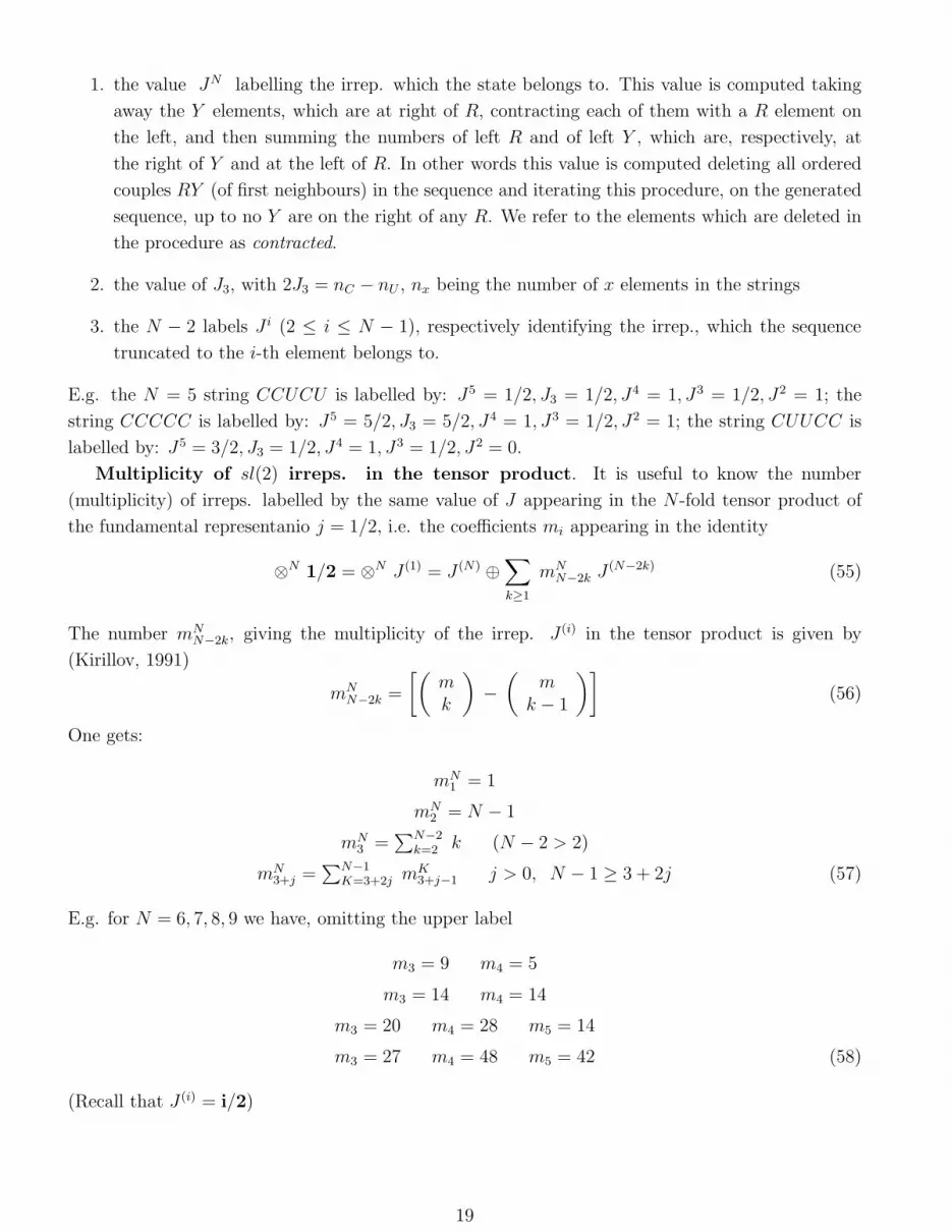
1. the value JN labelling the irrep. which the state belongs to. This value is computed taking

away the Y elements, which are at right of R, contracting each of them with a R element on

the left, and then summing the numbers of left R and of left Y , which are, respectively, at

the right of Y and at the left of R. In other words this value is computed deleting all ordered

couples RY (of first neighbours) in the sequence and iterating this procedure, on the generated

sequence, up to no Y are on the right of any R. We refer to the elements which are deleted in

the procedure as contracted.

2. the value of J3, with 2J3 = nC − nU , nx being the number of x elements in the strings

3. the N − 2 labels J i (2 ≤ i ≤ N − 1), respectively identifying the irrep., which the sequence

truncated to the i-th element belongs to.

E.g. the N = 5 string CCUCU is labelled by: J5 = 1/2, J3 = 1/2, J4 = 1, J3 = 1/2, J2 = 1; the

string CCCCC is labelled by: J5 = 5/2, J3 = 5/2, J4 = 1, J3 = 1/2, J2 = 1; the string CUUCC is

labelled by: J5 = 3/2, J3 = 1/2, J4 = 1, J3 = 1/2, J2 = 0.

Multiplicity of sl(2) irreps. in the tensor product. It is useful to know the number

(multiplicity) of irreps. labelled by the same value of J appearing in the N -fold tensor product of

the fundamental representanio j = 1/2, i.e. the coefficients mi appearing in the identity

⊗N 1/2 = ⊗N J (1) = J (N) ⊕∑

k≥1

mNN−2k J

(N−2k) (55)

The number mNN−2k, giving the multiplicity of the irrep. J (i) in the tensor product is given by

(Kirillov, 1991)

mNN−2k =

[(mk

)−

(m

k − 1

)](56)

One gets:

mN1 = 1

mN2 = N − 1

mN3 =

∑N−2k=2 k (N − 2 > 2)

mN3+j =

∑N−1K=3+2j m

K3+j−1 j > 0, N − 1 ≥ 3 + 2j (57)

E.g. for N = 6, 7, 8, 9 we have, omitting the upper label

m3 = 9 m4 = 5

m3 = 14 m4 = 14

m3 = 20 m4 = 28 m5 = 14

m3 = 27 m4 = 48 m5 = 42 (58)

(Recall that J (i) = i/2)

19

References

Arndt P.F., Burge C.B. and Hwa T., 2002, DNA Sequence Evolution with Neighbor-Dependent Muta-

tion, RECOMB2002, Proc. 6th Int.Conf. on Computational Biology (2002), p.32 (physics/0112029).

Blake R.D., Hess S.T. and Nicholson-Tuell J., 1992, The influence of Nearest Neighbors on the Rate

and Pattern of Spontaneous Mutations, J.Mol.Evol. 34, 189.

Blake R.D., Hess S.T. and Blake R.D., 1994, Wide Variations in Neighbor-dependent Substitution

Rates , J.Mol.Biol. 236, 1022.

Baake E., Baake M. and Wagner H., 1997, Ising quantum chain is equivalent to a model of biologi-

calevolution, Phys.Rev.Lett. 78 , 559; Erratum Phys.Rev.Lett. 79 , 1782.

Baake E., Baake M. and Wagner H., 1998, Quantum mechanics versus classical probability in biolog-

ical evolution, Phys.Rev. E 57, 1191.

Baake E. and Wagner H., 2001, Mutation-selection models solved exactly with methods of statistical

mechanics, Genet.Res.Camb. 78, 93.

Blake R.D., Hess S.T. and Nicholson-Tuell J., 1992, The Influence of Nearest Neighbors on the Rate

and Pattern of Spontaneous Point Mutation, J.Mol.Evol. 34, 189.

Eigen M., 1971, Selforganisation of matter and the evolution of biological macromolecules, Naturwis-

senschaften 58, 465.

Eigen M., McCaskill J. and Schuster P., 1989, The molecular quasi-species, J.Chem.Phys. 75, 149.

Encyclopedic Dictionary of Mathematics, 1960, 2nd edition, The MIT Press, Cambridge, (MA).

Frappat L., Sciarrino A. and Sorba P., 1998, A crystal basis model of the genetic code Phys. Lett.

A 250 214.

Frappat L., Sciarrino A. and Sorba P., 2001, Crystalizing the genetic code J.Biol. Phys. 27 1.

Frappat L., Minichini C., Sciarrino A. and Sorba P., 2003, Universality and Shannon Entropy for

Codon Usage Phys.Rev. E 68 , 061910.

Goldstein RF. and Benight A. S., 1992, How Many Numbers Are Required to Specify Sequence-

Dependent Properties of Polynucleotides?, Biopolymers 32, 1679.

Hermisson J., Wagner H. and Baake M., 2001, Four-State Quantum Chain as a Model of Sequence

Evolution, J.Stat.Phys. 102, 315.

Hermisson J., Redner O. , Wagner H. and Baake E., 2002, textitMutation-selection balance: Ancestry,

load and maximum priciple, Theoretical Population Biology 62, 9.

Hess S.T., Blake J.D. and Blake R.D., 1994, Wide Variations in Neighbor-dependent Substitution

Rates, J.Mol.Evol. 236, 1022.

Hofbauer J. and Sigmund K., 1988, The Theory of Evolution and Dynamical Systems. Cambridge

University Press, Cambridge.

Kashiwara M., 1990, Crystallizing the q-analogue of universal enveloping algebras, Commun. Math.

Phys. 133 249.

20

Kirillov A.A., 1991, Representation theory and Noncommutative Harmonic Analysisis, Encyclopedia

of Mathematical Sciences, Vol. 22, pag. 70, Springer Verla, Berlin.

Leuthausser I., 1986, An exact correspondence between Eigen’s evolution model and a two-dimensional

Ising system, J.Chem.Phys. 84, 1884.

Leuthausser I., 1987, Statistical mechanics of Eigen’s evolution model, J.Stat.Phys. 48, 343.

Li Wen-Hsiung, 1997, Molecular Evolution, Sinauer Associates Incorporated, Sunderland.

Martindale C. and Konopka A. K., 1996, Oligonucleotide Frequencies in DNA Follow a Yule Distri-

butiojn, Computers Chem. 20, 35.

Minichini C. and Sciarrino A., 2004a, Quantum Spin Model fitting the Yule distribution of oligonu-

cleotides , quant-ph/0409071

Minichini C. and Sciarrino A., 2004b, Mutation Model fitting the Yule distribution of oligonu-

cleotides, q-bio.BM/0412006

Saakian S. and Hu Chin-Kun, 2004, Eigen Model as a Quantum Spin Chain: Exact Dynamics,

Phys.Rev. E 69, 021913 (cond-mat/0402212).

SantaLucia, J., 1998, A unified view of polymer, dumbbell, and oligonucleotide DNA nearest-neighbor

thermodynamics, Proc.Natl.Acad.Sci USA 95, 1460.

Wagner H., Baake E. and Gerisch T., 1998, Ising quantum chain and sequence evolution, J.Stat.Phys.

92 , 1017.

Whelan S. and Goldman N., 2004, Estimating the Frequency of Events That Cause Multiple-Nucleotide

Changes, Genetics 167, 2027.

Xia Tiambing et al, 1998, Thermodynamic Parameters for an Expanded Nearest-Neighbor Model for

Formation of RNA Duplexes with Watson-Crick Base Pairs, Biochemistry 37, 14719.

Yule G.U., 1924, A mathematical theory of evolution, based on the conclusions of Dr.J.C. Willis,

F.R.S., Phil.Trans. B 213, 21.

Zipf, G.K., 1949 Human behaviour and the Principle of Least Effort, Addison-Wesley Press, Cam-

bridge, MA .

21

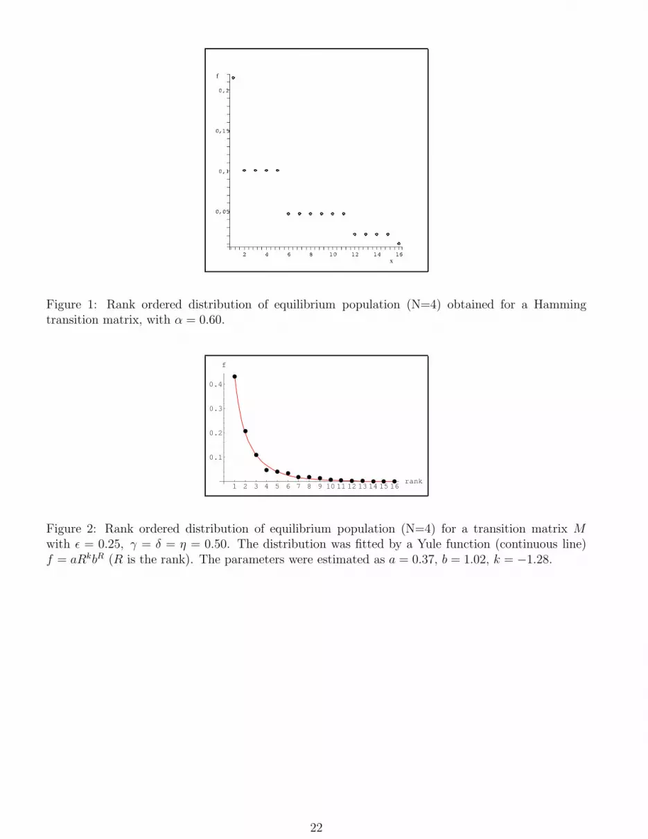
Figure 1: Rank ordered distribution of equilibrium population (N=4) obtained for a Hammingtransition matrix, with α = 0.60.

1 2 3 4 5 6 7 8 9 10 11 12 13 14 15 16rank

0.1

0.2

0.3

0.4

f

Figure 2: Rank ordered distribution of equilibrium population (N=4) for a transition matrix Mwith ǫ = 0.25, γ = δ = η = 0.50. The distribution was fitted by a Yule function (continuous line)f = aRkbR (R is the rank). The parameters were estimated as a = 0.37, b = 1.02, k = −1.28.

22

0 10 20 30 40 50 60rank

0.02

0.04

0.06

0.08

0.1

f

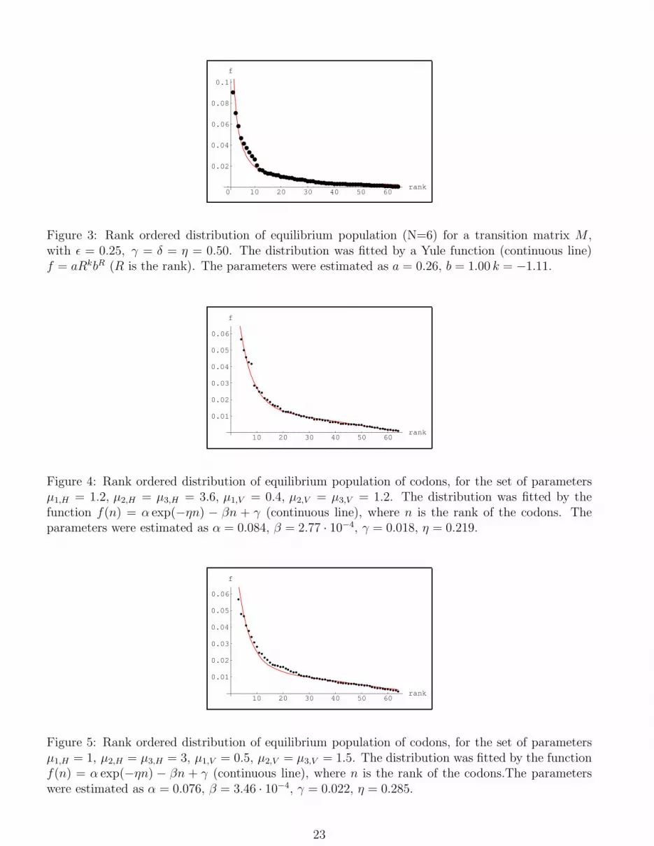
Figure 3: Rank ordered distribution of equilibrium population (N=6) for a transition matrix M ,with ǫ = 0.25, γ = δ = η = 0.50. The distribution was fitted by a Yule function (continuous line)f = aRkbR (R is the rank). The parameters were estimated as a = 0.26, b = 1.00 k = −1.11.

10 20 30 40 50 60rank

0.01

0.02

0.03

0.04

0.05

0.06

f

Figure 4: Rank ordered distribution of equilibrium population of codons, for the set of parametersµ1,H = 1.2, µ2,H = µ3,H = 3.6, µ1,V = 0.4, µ2,V = µ3,V = 1.2. The distribution was fitted by thefunction f(n) = α exp(−ηn) − βn + γ (continuous line), where n is the rank of the codons. Theparameters were estimated as α = 0.084, β = 2.77 · 10−4, γ = 0.018, η = 0.219.

10 20 30 40 50 60rank

0.01

0.02

0.03

0.04

0.05

0.06

f

Figure 5: Rank ordered distribution of equilibrium population of codons, for the set of parametersµ1,H = 1, µ2,H = µ3,H = 3, µ1,V = 0.5, µ2,V = µ3,V = 1.5. The distribution was fitted by the functionf(n) = α exp(−ηn) − βn + γ (continuous line), where n is the rank of the codons.The parameterswere estimated as α = 0.076, β = 3.46 · 10−4, γ = 0.022, η = 0.285.

23

10 20 30 40 50 60rank

0.01

0.02

0.03

0.04

0.05

0.06

f

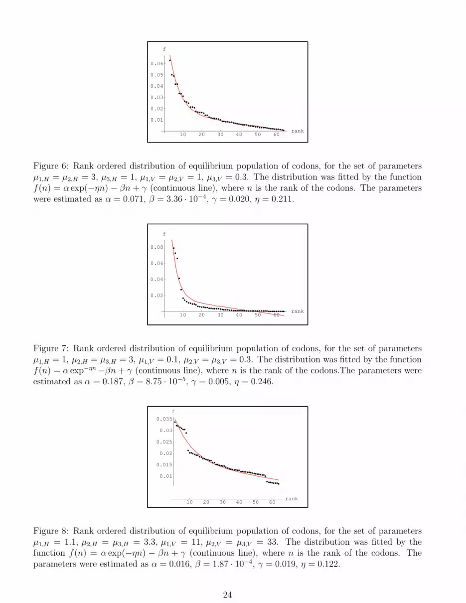
Figure 6: Rank ordered distribution of equilibrium population of codons, for the set of parametersµ1,H = µ2,H = 3, µ3,H = 1, µ1,V = µ2,V = 1, µ3,V = 0.3. The distribution was fitted by the functionf(n) = α exp(−ηn) − βn + γ (continuous line), where n is the rank of the codons. The parameterswere estimated as α = 0.071, β = 3.36 · 10−4, γ = 0.020, η = 0.211.

10 20 30 40 50 60rank

0.02

0.04

0.06

0.08

f

Figure 7: Rank ordered distribution of equilibrium population of codons, for the set of parametersµ1,H = 1, µ2,H = µ3,H = 3, µ1,V = 0.1, µ2,V = µ3,V = 0.3. The distribution was fitted by the functionf(n) = α exp−ηn −βn + γ (continuous line), where n is the rank of the codons.The parameters wereestimated as α = 0.187, β = 8.75 · 10−5, γ = 0.005, η = 0.246.

10 20 30 40 50 60rank

0.01

0.015

0.02

0.025

0.03

0.035

f

Figure 8: Rank ordered distribution of equilibrium population of codons, for the set of parametersµ1,H = 1.1, µ2,H = µ3,H = 3.3, µ1,V = 11, µ2,V = µ3,V = 33. The distribution was fitted by thefunction f(n) = α exp(−ηn) − βn + γ (continuous line), where n is the rank of the codons. Theparameters were estimated as α = 0.016, β = 1.87 · 10−4, γ = 0.019, η = 0.122.

24

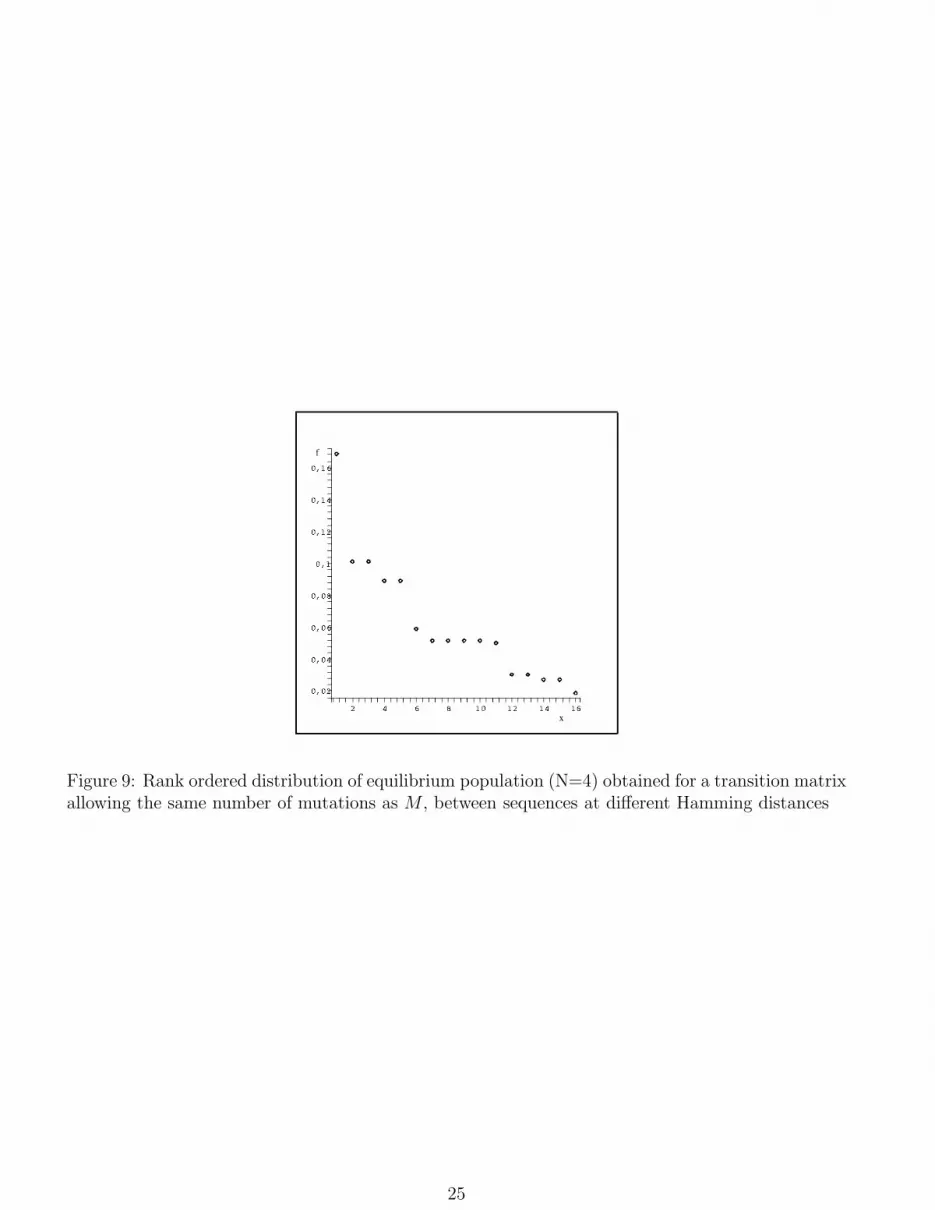
Figure 9: Rank ordered distribution of equilibrium population (N=4) obtained for a transition matrixallowing the same number of mutations as M , between sequences at different Hamming distances

25