Must Try Harder: Evaluating the Role of Effort in Educational Attainment

DISCUSSION PAPER SERIES

ABCD

www.cepr.org

Available online at: www.cepr.org/pubs/dps/DP5048.asp and www.ssrn.com/abstract=774304

www.ssrn.com/xxx/xxx/xxx

No. 5048

MUST TRY HARDER. EVALUATING

THE ROLE OF EFFORT IN EDUCATIONAL ATTAINMENT

Gianni De Fraja, Tania Oliveira and Luisa Zanchi

PUBLIC POLICY

ISSN 0265-8003

MUST TRY HARDER. EVALUATING THE ROLE OF EFFORT IN

EDUCATIONAL ATTAINMENT

Gianni De Fraja, University of Leicester and CEPR Tania Oliveira, University of Leicester

Luisa Zanchi, University of Leeds

Discussion Paper No. 5048 May 2005

Centre for Economic Policy Research 90–98 Goswell Rd, London EC1V 7RR, UK

Tel: (44 20) 7878 2900, Fax: (44 20) 7878 2999 Email: [email protected], Website: www.cepr.org

This Discussion Paper is issued under the auspices of the Centre’s research programme in PUBLIC POLICY. Any opinions expressed here are those of the author(s) and not those of the Centre for Economic Policy Research. Research disseminated by CEPR may include views on policy, but the Centre itself takes no institutional policy positions.

The Centre for Economic Policy Research was established in 1983 as a private educational charity, to promote independent analysis and public discussion of open economies and the relations among them. It is pluralist and non-partisan, bringing economic research to bear on the analysis of medium- and long-run policy questions. Institutional (core) finance for the Centre has been provided through major grants from the Economic and Social Research Council, under which an ESRC Resource Centre operates within CEPR; the Esmée Fairbairn Charitable Trust; and the Bank of England. These organizations do not give prior review to the Centre’s publications, nor do they necessarily endorse the views expressed therein.

These Discussion Papers often represent preliminary or incomplete work, circulated to encourage discussion and comment. Citation and use of such a paper should take account of its provisional character.

Copyright: Gianni De Fraja, Tania Oliveira and Luisa Zanchi

CEPR Discussion Paper No. 5048

May 2005

ABSTRACT

Must Try Harder. Evaluating the Role of Effort in Educational Attainment*

This paper is based on the idea that the effort exerted by children, parents and schools affects the outcome of the education process. We test this idea using the National Child Development Study. Our theoretical model suggests that the effort exerted by the three groups of agents is simultaneously determined as a Nash equilibrium, and is therefore endogenous in the estimation of the education production function. Our results support this, and indicate which factors affect examination results directly and which indirectly via effort; they also suggest that affecting effort directly has an impact on results.

JEL Classification: I220 and H420 Keywords: educational achievement, educational attainment, educational outcomes, effort at school and examination results

Gianni De Fraja Department of Economics University of Leicester Leicester LE1 7RH Tel: (44 116) 252 3909 Fax: (44 116) 252 2908 Email: [email protected] For further Discussion Papers by this author see: www.cepr.org/pubs/new-dps/dplist.asp?authorid=113071

Tania Oliveira Department of Economics University of Leicester University Road Leicester LE1 7RH Email: [email protected] For further Discussion Papers by this author see: www.cepr.org/pubs/new-dps/dplist.asp?authorid=162519

Luisa Zanchi Economics Division Leeds University Business School EES Building University of Leeds Leeds LS2 9JT Tel: (44 113) 233 4464 Fax: (44 113) 233 4465 Email: [email protected] For further Discussion Papers by this author see: www.cepr.org/pubs/new-dps/dplist.asp?authorid=150050

*We would like to thank Karim Abadir, Sarah Brown, Gabriele Fiorentini, Andrea Ichino, Andrew Jones, Steve Machin, Kevin Reilly, Karl Taylor, and the audience at the Education Department in Leicester for helpful suggestions and comments on an earlier draft.

Submitted 13 April 2005

NON-TECHNICAL SUMMARY

This paper is based on the very simple observation that the educational attainment of students is affected by the effort put in by those participating in the education process: the schools attended by the students, the students' parents, and of course the students themselves. Although psychologists and educationalists have long acknowledged the importance of schools’, parents’ and students’ effort, the economic literature on educational achievement has so far paid only limited attention to the role of effort as a separate input to the education process, both at a theoretical and at an empirical level.

We build a theoretical model where educational attainment is positively affected by students’, parents’ and schools’ effort and where the effort of these three groups of agents is jointly determined: students respond to the effort exerted by their parents and their schools, and, correspondingly, schools respond to the effort exerted by their students and their parents, and parents to the effort exerted by their children and their children's schools. All agents have a common interest in the realisation of the best educational outcome for the students, but the complex interactions among them may lead to counterintuitive results. For example, students may respond to an increase in school effort with a lower level of their own effort.

We then estimate the theoretical model using the National Child Development Study, a very rich dataset which follows a cohort of individuals born in 1958, from birth until the age of 42. We use information obtained by comprehensive questionnaires completed when the individuals were 7, 11, and 16. We also have detailed results of all examinations taken up to the age of 20. We construct our measures of effort using many indicators of a student's, her parents’ and her school’s attitudes. For students, for example, we use the answers given by 16-year-olds to questions such as whether they think that school is a ''waste of time'', and the teacher's views about the students' laziness. Other questions regard the parents' interest in their children's education, measured, for example, by whether they read to their children or attend meetings with teachers, and the teacher's perception of this interest. For schools we use variables such as the extent of parental involvement initiated by the school, whether 16-year old students are offered career guidance, and the type of disciplinary methods employed. We also include many other standard explanatory variables. These can refer to individual, family, or school characteristics, as well as geographical indicators. They comprise the students’ ability, measured by administered tests independent of formal examinations and taken at the ages of 7, 11 and 16, the parents’ social class and education, and the type of school, whether state or private.

Our empirical estimates seem to confirm our theoretical prediction of joint determination of the effort levels of the three groups of agents. Moreover, our measures of effort seem appropriate, especially so for students and parents. For example, we find a trade-off between the quantity of children and their parents’ effort: a child's number of siblings affects negatively the effort exerted by that child's parents towards that child's education. Our econometric model allows us to determine whether explanatory variables influence educational attainment directly, or indirectly by affecting effort. For example, our results suggest that family socio-economic conditions influence attainment more strongly via effort than directly. In this case, policies that attempt to stimulate parental effort might be effective ways to improve the educational attainment. Affecting parental effort is likely to be easier than modifying social background. We also find that the children's own effort has the least important effect on educational attainment: schools and parents matter more. Interestingly, the school's effort matters more than the parents' for girls, and, vice versa, it matters less than the parents' for boys. This may provide an explanation for the recent trend of improvement in educational achievement, a trend which is stronger for girls than for boys in the UK, and which is occurring at a time when increasing attention is paid to schools’ results, and to the provision of financial incentives to schools and teachers. To the extent that these incentives stimulate schools' effort, our analysis indicates that girls' educational attainment should improve more than boys’.

1 Introduction

This paper is based on a very simple idea: the educational achievement of a

student is affected by the effort put in by those participating in the educa-

tion process: schools, parents, and of course the students themselves. This is

natural, and indeed psychologists and educationalists have long been aware of

the importance of effort for educational attainment. Student’s effort is usually

proxied by the amount of homework undertaken that is unconstrained by the

scheduling practices of the schools (Natriello and McDill (1986)). However,

empirical research in this area is still far from reaching clear conclusions. This

is due partly to ambiguities in the interpretation of homework: it could be seen

as an indicator of either students’ effort, operating at the individual level, or

teachers’ effort, operating at the class level (Trautwein and Köller (2003)). As

well as students’ effort, the educational psychology literature has also studied

the relationship between school attainment and parental effort. A variety of

dimensions of parental effort has been considered, ranging from parents’ ed-

ucational aspirations for their children, to parent-child communication about

school matters, to education-related parental supervision at home, and to par-

ents’ participation in school activities. As Fan and Chen (2001) note, much

of this literature is qualitative rather than quantitative and most of the quan-

titative studies rely on simple bivariate correlations rather than on regression

analysis. Results are not clear-cut here either: if at all, parental effort appears

to affect educational attainment only indirectly, to the extent that it supports

children’s effort (Hoover-Dempsey et al. (2001)).

The lack of specific data quantifying effort as a separate variable affect-

ing educational attainmenthas also hindered studies carried out by economists.

For example, Hanushek (1992) proxies parental effort with measures of fam-

ily socio-economic status (permanent income and parents’ education levels).

Intuition — confirmed by our results — would however suggest that effort and

socio-economic conditions are in fact distinct variables. Indeed, Becker and

Tomes’ (1976) theoretical model of optimal parental time allocation suggests a

negative relationship between household income and parental effort.1 Bones-

røning (1998; 2004) and Cooley (2004) are among the very few authors in the

economics literature who measure the effort exerted by students and parents1Their idea is that parents try to maximise the welfare of their children, and they may

decide to allocate more time and effort to their children’s education if they perceive limitsto their ability to transfer income through inheritance; this is more likely to be the case forlow-income families.

1

and estimate its effects on examination results.

Theoretical analyses of the role of effort in the education process are also

scarce.2 Our paper attempts to fill this gap, by developing a theoretical model

of the determination as a Nash equilibrium of the effort exerted by students,

their parents and their schools, and subsequently by estimating empirically the

determinants of the effort levels, the interaction among of them, and the effect

of effort on educational attainment.

We test the theoretical model with the British National Child Development

Study (NCDS). This is a well suited dataset, as it contains a large number of

variables which can be used as indicators of effort: there are variables which

denote a student’s attitude, for example whether they think that school is a

“waste of time”, and the teacher’s views about the student’s laziness. Other

questions regard the parents’ interest in their children’s education, whether

they read to their children or attend meetings with teachers, and the teacher’s

perception of this interest. For schools, we use variables such as the extent of

parental involvement initiated by the school, whether 16-year old students are

offered career guidance, and the type of disciplinary methods used.

Our empirical estimates of the determinants of effort are encouraging: the

theoretical assumption of joint interaction of the effort levels of the three groups

of agents appears to be borne out by the data. Moreover, our measures of effort

seem appropriate, especially so for children and parents. For example, as a by-

product of our analysis, we find confirmation of Becker’s (1960) intuition that

there is a trade-off between quantity and quality of children: a child’s number

of siblings influences the effort exerted by that child’s parents towards that

child’s education.

Our econometric model allows us to determine whether explanatory vari-

ables influence educational attainment directly or indirectly, that is by affecting

effort. For example, our results suggest that family socio-economic conditions

affect attainment more strongly via effort than directly. In this case, policies2This contrasts sharply with the extensive literature which studies the role of effort in

firms; a seminal contribution is the theory of efficiency wages (Shapiro and Stiglitz (1984)),and an extensive survey is provided by Holmstrom and Tirole (1989). There have also beenseveral attempts to estimate empirically the role of effort in firms: an early test of the efficiencywage hypothesis is Cappelli and Chauvin (1991), who measured workers’ effort by disciplinarydismissals. More recently, effort has been measured by the propensity to quit (Galizzi andLang (1998)), by misconduct (Ichino and Maggi (2000)) and by absenteeism (Ichino andRiphahan (2004)). Peer pressure, measured by the presence of a co-worker in the same room,also appears to affect a worker’s effort (Falk and Ichino (2003)).

2

that attempt to affect parental effort might be effective ways to improve the

educational attainment, since affecting parental effort is likely to be easier than

modifying social background.3 We also find that the children’s own effort has

the least effect on educational attainment: schools and parents are more im-

portant. Interestingly, the school’s effort matters more than the parents’ for

girls, and, vice versa, it matters less than the parents’ for boys (see Figure

4 below). This may provide an explanation for the recent trend of improve-

ment in the education achievement in the UK, a trend which is stronger for

girls than for boys, and which is happening when increasing attention is being

paid to schools’ results, and financial incentives are being provided to schools

and teachers. To the extent that these incentives stimulate the schools’ effort,

our results indicate that girls’ education attainment should improve more than

boys.

The paper is organised as follows: the theoretical model is developed in

Section 2; the agents’ strategic behaviour is illustrated in Section 3 with a

graphical analysis of the Nash equilibrium; the empirical model is presented in

Section 4; Section 5 describes the data and the variables used; our results are

summarised in Section 6, and concluding remarks are in the last section.

2 Theoretical Model

We model the interaction among the pupils at a school, their teachers and

their parents. Pupils attend school, and, at the appropriate age, they leave

with a qualification. This is a variable q taking one of m possible values

q ∈ {q1, ..., qm}, with qk−1 < qk, k = 2, ...,m. Other things equal, a stu-

dent prefers a better qualification: apart from personal satisfaction, there is

substantial evidence showing a positive association between qualification and

future earnings in the labour market: let u (q) be the utility associated with

qualification q, with u0 (q) > 0.

When at school, pupils exert effort, which we denote by eC ∈ EC ⊆ IR (thesuperscript C stands for “child”). The restriction to single dimensionality is

made for algebraic convenience, though it is also supported by the data, see

Section 6 below. eC measures how diligent a pupil is, how hard she works and

so on, and has a utility cost measured by a function ψC¡eC¢, increasing and

3One example could be the provision of direct financial rewards to parents helping theirchildren with homework, or attending parenting classes, similarly to the policy of providing fi-nancial incentives to disadvantaged teen-agers for staying on at school beyond the compulsoryage (Dearden et al. (2003)).

3

convex: ψ0C¡eC¢,ψ00C

¡eC¢> 0. Notice that there is no natural scale to measure

effort, and so the interpretation of the function ψC (and the corresponding ones

for schools and parents), is cost of effort relative to the benefit of qualification.

Pupils also differ in ability, denoted by a. A student’s education attainment is

affected by her effort and her ability. Formally, we assume that qualification qkis obtained with probability πk

¡eC , a; ·

¢(the “ · ” represents other influences on

qualification, discussed in what follows). We hypothesise, naturally, a positive

relationship between effort and the expected qualification:Pmk=1

∂πk(eC ,a;·)∂eC

qk >

0, and between ability and the expected qualification:Pmk=1

∂πk(eC ,a;·)∂a qk > 0.

A student’s objective function is the maximisation of the difference between

expected utility and the cost of effort:

mXk=1

πk¡eC , a; ·

¢u (qk)− ψC

¡eC¢. (1)

A student’s education attainment depends also on her parents’ effort. Par-

ents may help with the homework, provide educational experiences (such as

museums instead of television), take time to speak to their children’s teachers,

and so on: we denote this effort by eP ∈ EP ⊆ IR; as before, this is treated assingle dimensional. Consistently with common sense, and with the idea that

the education process is best thought of as a long term process (e.g. Hanushek

(1986) and Carneiro and Heckman (2003)), the variable eP should be viewed

as summarising the influence of parental effort throughout the child’s school

career: the NCDS dataset is well suited to take on board this view, as each

subject is observed at three dates, at age 7, at age 11 and at age 16. Par-

ents differ also in education, social background and other variable which affect

their children’s education attainment; we capture this by means of a possibly

multidimensional variable, sP .

Parents care about their children’s qualification, and so they will exert effort

eP , even though it carries a utility cost, measured by the function ψP¡eP¢,

increasing and convex: ψ0P¡eP¢,ψ00P

¡eP¢> 0. Parents may have more than

one child and so they care about the average qualification of all their children:4

4Rigorously, we should consider the utility of the qualification, for example uP (q). It is notin general obvious which shape the function uP (q) should have: some parents may obtain ahigher utility gain if the qualification of a less bright child is increased, than if the qualificationof a more able child is increased equivalently; other parents, who value achieving excellencemore than avoinding failure may take an opposite view; given this potential ambiguity, itseems a good approximation to take the average attainment as the objective function.

4

if parents have n children, their payoff function is given by:

nXj=1

πk¡eCj , aj ; e

Pj , s

P ; ·¢qk − ψP

³Pnj=1 e

Pj

´,

where ePj is the effort devoted by parents to child j, whose ability is aj , and

who exerts effort eCj .5

A student’s qualification will also be affected by the quality of her school,

the last component of the “ · ” in the arguments of the probabilities in (1). Theschool influences its pupils’ attainment through its own effort, measured by a

variable eS ∈ ES ⊆ IR (again assumed one-dimensional). This captures the

idea that a school can take actions which affect the quality of the education it

imparts. Improving the quality of buildings, classroom equipment and sporting

facilities, using computers appropriately, upgrading teachers’ qualifications are

all examples. Other examples are the teachers’ interest and enthusiasm in their

classroom activities, the time they spend outside teaching hours to prepare

lessons, to assess the students’ work, to meet parents, and so on.6 Effort has

increasing marginal disutility, and can thus be measured by a function ψS¡eS¢

increasing and convex, ψ0S¡eS¢,ψ00S

¡eS¢> 0.

To wrap up this discussion, the probability that a student obtains qualifi-

cation qk can therefore be written as

πk¡eC , a; eP , sP ; eS , sS

¢,

where, in analogy to sP , sS is a vector which captures the school’s exogenously

given characteristics. A school’s objective function is a function which depends

positively on the average7 qualification of its students and negatively on the5The interaction between parental effort and the number of children was first proposed by

Becker (1960). We ignore the potential endogeneity of the number of children. Blake (1989)is a demographic analysis of the relationship between family size and achievement.

6Note that the activities in the first group are fixed before the students are enrolled atschool and can therefore be observed by parents prior to applying to the school; while thosein the second group are carried out once the students are at school. Since the extent ofschool choice was fairly limited in the period covered by our data, this distinction will bedisregarded in what follows. The theoretical analysis of De Fraja and Landeras (2005) arguesthat a different equilibrium concept should be used according to whether schools and studentschoose one after the other or simultaneously: Stackelberg and Nash equilibrium respectively.As they show, this does not affect the qualitative nature of the interaction.

7As with parents, the average qualification may not be the most suitable approximationfor the school’s objective function. Teachers may care more about the best or the weakeststudents in their class. If this were the case, appropriate weighting could be included toaccount for these biases in the school’s payoff function (2).

5

teaching effort:

mXk=1

qk

HXh=1

πk¡eC (h) , a; eP (h) , sP ; eS (h) , sS

¢λh − ψS

¡eS¢. (2)

(2) assumes that the effort levels eC , eP , and eS are affected by a number of

exogenous variables described by the multi-dimensional vector h: thus eC (h)

(respectively eP (h), respectively eS (h)) is the effort level exerted by students

(respectively parents, respectively schools) whose vector of relevant variables

takes value h. h will of course also include ability and other variables which are

also in the vectors sP and sS , as these can have a direct effect on qualification,

or an indirect effect, via the effort level exerted by the participants in the

education process. H is the number of all the possible values which the variables

affecting effort can take, and λh is the proportion of pupils at the school with

this variable equal to h.

Additivity between the disutility of effort and the students’ average qual-

ification is an innocuous normalisation. The relative importance of these two

components of the school’s utility will in general depend on how much teachers

care about the success of their pupils, which in turn can depend on government

policy: there could be incentives for successful teachers (both monetary and in

terms of improved career prospects; De Fraja and Landeras’s (2005) theoret-

ical model studies the effects of strengthening these incentives). The dataset

we have available, which refers to schools in the late ’60s and early ’70s is not

suited to the study of these effects, since there has been no observable change

in the power of the incentive schemes for schools and teachers in that period.

3 A graphical analysis of the equilibrium

All agents have a common interest in the realisation of a high qualification

for the child, but their interests are not perfectly aligned, and their strategic

behaviour may lead to complex interactions among them, with counterintuitive

outcomes.

In this brief section we illustrate this point in an extremely simple case.

We assume that all students in a given school are identical in terms of ability,

parental status, and number of siblings. This is obviously unrealistic, but

the point here is to illustrate that, even with highly special assumptions, the

interaction between the parties may turn out to be extremely complex. We

capture this interaction with the game theoretic concept of Nash equilibrium:

6

each party is choosing their effort in order to maximise their utility, taking as

given the choice of effort of the other parties. An equilibrium is given by the

set of values eC , eP , and eS, satisfying the first order conditions

mXk=1

u (qk)∂πk

¡eC , a; eP , sP ; eS , sS

¢∂eC

− ψ0C¡eC¢= 0, (3)

mXk=1

qk∂πk

¡eC , a; eP , sP ; eS, sS

¢∂eP

− ψ0P¡eP¢= 0, (4)

mXk=1

qk∂πk

¡eC , a; eP , sP ; eS, sS

¢∂eS

− ψ0S¡eS¢= 0. (5)

where the appropriate second order conditions are satisfied. (3)-(5) are the

best reply function8 of each of the three agents: their intersections identify the

Nash equilibria. The graphical analysis is best conducted in two dimensions.

Let therefore the parental effort be fixed, at eP . Total differentiation of (3) and

(5) gives the slope of the best reply function in the relevant Cartesian diagram

(EC ×ES for fixed eP ):ÃmXk=1

u (qk)∂2πk (·)∂eC∂eS

!deS − U 00C (·) deC = 0,Ã

mXk=1

qk∂2πk (·)∂eC∂eS

!deC − U 00S (·) deS = 0,

where U 00C (·) =Pmk=1 u (qk)

∂2πk(·)(∂eC)2

− ψ00C¡eC¢< 0 is the second derivative of

the child’s payoff, and analogously for U 00S (·). From the above:

deS

deC

¯̄̄̄childBRF

=U 00C (·)Pm

k=1 u (qk)∂2πk(·)∂eC∂eS

, (6)

deS

deC

¯̄̄̄schoolBRF

=

Pmk=1 qk

∂2πk(·)∂eC∂eS

U 00S (·). (7)

8Mathematically, for the representative student (that the we can take a representativestudent is shown in De Fraja and Landeras (2005)), this is a function from the product of theother two effort spaces into the child’s: EP ×ES −→ EC . This a dimension 2-manifold in the3-dimensional Cartesian space EC × EP × ES . Analogously for the parents and the school.The intersection of three dimension 2-manifolds is (generically) either empty, or a dimension0-manifold, that is a set of isolated points. Existence of at least one Nash equilibrium isensured by the fact that each player has a compact and convex strategy space, and thattheir payoff functions are continuous and quasi-concave in their own strategy (Fudenberg andTirole 1991, p 34).

7

e

school’s best reply function

student’s best reply function

panel (a) panel (b)

C

eS

e

school’s best reply function

student’s best reply function

C

eS

E0

E1

E0

E1

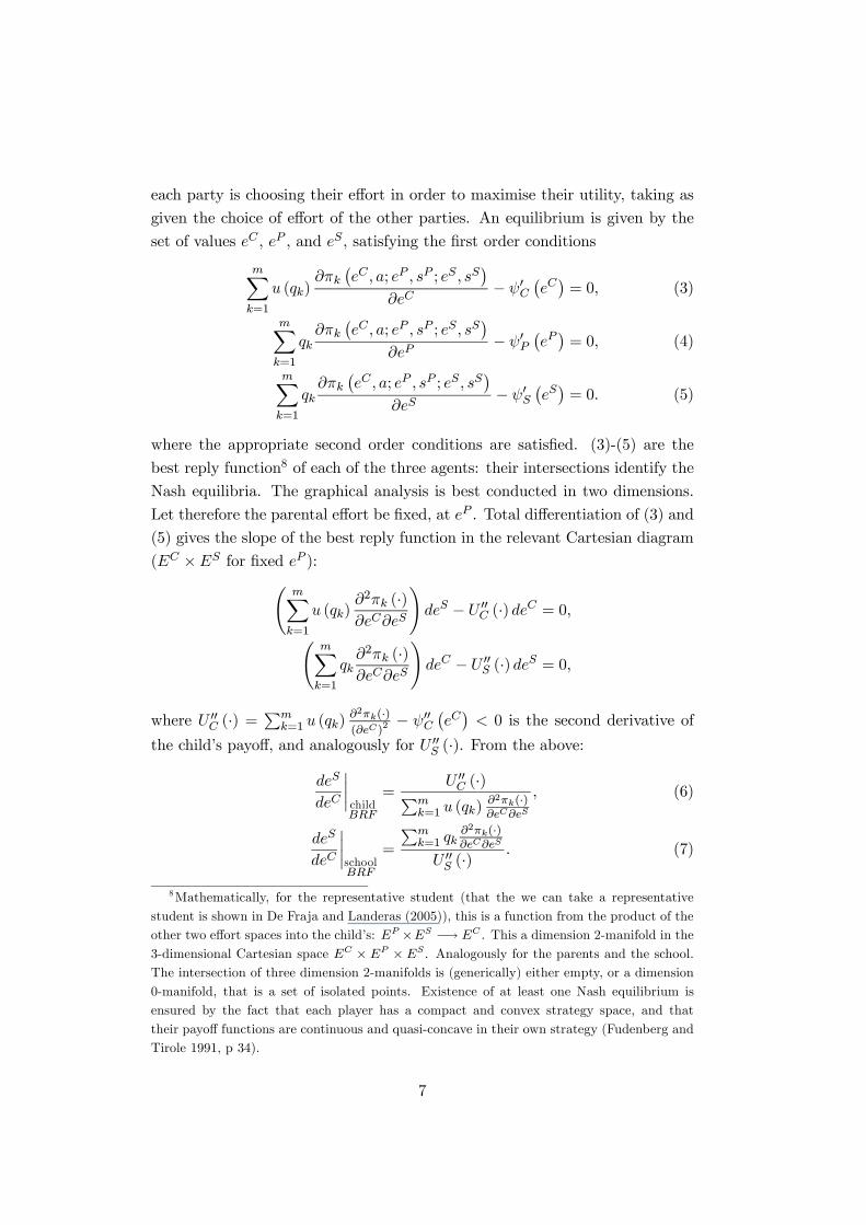
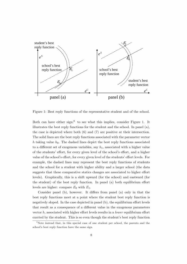
Figure 1: Best reply functions of the representative student and of the school.

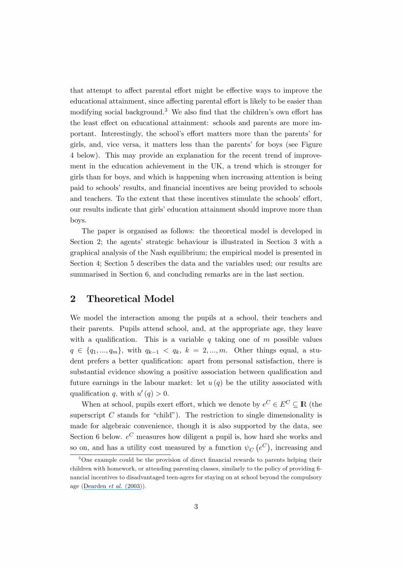
Both can have either sign:9 to see what this implies, consider Figure 1. It

illustrates the best reply functions for the student and the school. In panel (a),

the case is depicted where both (6) and (7) are positive at their intersection.

The solid lines are the best reply functions associated with the parameter vector

h taking value h0. The dashed lines depict the best reply functions associated

to a different set of exogenous variables, say h1, associated with a higher value

of the students’ effort, for every given level of the school’s effort, and a higher

value of the school’s effort, for every given level of the students’ effort levels. For

example, the dashed lines may represent the best reply functions of students

and the school for a student with higher ability and a larger school (the data

suggests that these comparative statics changes are associated to higher effort

levels). Graphically, this is a shift upward (for the school) and eastward (for

the student) of the best reply function. In panel (a) both equilibrium effort

levels are higher: compare E0 with E1.

Consider panel (b), however. It differs from panel (a) only in that the

best reply functions meet at a point where the student best reply function is

negatively sloped. In the case depicted in panel (b), the equilibrium effort levels

that result as a consequence of a different value in the exogenous parameters

vector h, associated with higher effort levels results in a lower equilibrium effort

exerted by the student. This is so even though the student’s best reply function9Note instead that, in this special case of one student per school, the parents and the

school’s best reply function have the same sign.

8

shifts eastward: h1 is associated to higher values in the student’s effort for any

given level of the school’s effort. The reason for the lower equilibrium value

of the student’s effort is the strategic interaction of schools and students. The

vector h1 would be associated to a higher value of the student’s effort if the

school’s effort were the same. However, the student’s and the school’s efforts

are “strategic substitutes” (Bulow et al 1986), and the student responds to the

higher school effort (associated to the vector h1) with a lower level of their

own effort. This, in panel (b) in the diagram, more than compensates the

direct increase in the student’s effort caused by the different value of h. This

simple example illustrates the potential ambiguity of changes in the exogenous

variables h on the equilibrium effort levels; in more general settings the situation

will be even more complex.

4 Empirical Model

Given this theoretical ambiguity, the overall effect of children’s, parents’ and

school’s efforts on educational attainment, and whether these effort levels are

strategic complements or substitutes, is therefore largely an empirical matter,

to which we turn in this section.

The educational outcome variable considered here, Qi, is child i’s academic

results over a number of secondary school examinations, normally taken be-

tween the ages of 16 and 18. The explanatory variables are measures of the

effort exerted by the child, her parents and her school, and a suitable set of

controls for heterogeneity in socio-economic, demographic and other relevant

factors. Formally, the academic achievement is specified as:

Qi = xQ0i β1 + β2e

Ci + β3e

Pi + β4e

Si + ui, i = 1, ..., n, (8)

where xQi is a set of control variables for demographic and socio-economic

background factors affecting the educational outcome, eCi , ePi , and e

Si are the

measures of the effort exerted by child i, by child i’s parents and by child i’s

school, and ui the error term.

Our theoretical analysis in Sections 2 and 3 suggests that the interaction

between the three types of agents is best captured as a Nash equilibrium. This

implies that the effort levels, which are educational inputs, simultaneously de-

termine each other; together with possible omitted variables, this in turn im-

plies that the error term in the estimation of a standard educational production

function (Hanushek (1986) is correlated with the observed input variables and

9

the estimates of the effect of observed inputs on educational outcome are incon-

sistent. The very rich set of background variables in our dataset should lessen

the problem of omitted variables.

To address the endogeneity of the effort variables, note that the interde-

pendent system:

eCi = xC0i γ

C1 + γC2 e

Pi + γC3 e

Si + v

Ci , i = 1, ..., n, (9)

ePi = xP 0i γ

P1 + γP2 e

Ci + γP3 e

Si + v

Pi , i = 1, ..., n, (10)

eSi = xS0i γ

S1 + γS2 e

Ci + γS3 e

Pi + v

Si , i = 1, ..., n, (11)

is a linear approximation to the Nash equilibrium. In (9)-(11), xCi , xPi and x

Si

are the background factors affecting child i’s effort, child i’s parents’ effort, and

the effort of child i’s school, respectively, and vCi , vPi and v

Si are error terms,

possibly correlated.

The NCDS dataset contains many variables that capture aspects of indi-

vidual effort levels, eCi , ePi and e

Si . Described in detail in Section 5, these take

the form of categorical variables, which have different scales and are in gen-

eral non-comparable. We therefore use factor analysis10 to construct a single

aggregate continuous indicator of the three effort levels.

We next need to ascertain whether the effort variables are endogenous as

suggested in Sections 2 and 3. We do so using the Durbin-Wu-Hausman (DWH)

augmented regression test suggested by Davidson and MacKinnon (1993). The

test is performed by obtaining the residuals from a model of each endogenous

right-hand side variable as a function of all exogenous variables, and including

these residuals in a regression of the original model. In our case, we first

estimate the system

eCi = exC0i δC1 + δC2 ePi + δC3 e

Si + r

Ci , (12)

ePi = exP 0i δP1 + δP2 eCi + δP3 e

Si + r

Pi , (13)

eSi = exS0i δS1 + δS2 eCi + δS3 e

Pi + r

Si , (14)

10We use the principal factor method. Alternative approaches include principal compo-nents, principal-components factor analysis and maximum-likelihood factor analysis (Harman(1976), Everitt and Dunn (2001)). Since our original variables are defined on an ordinal ratherthan an interval scale, they are not suited to being analysed by the maximum-likelihood fac-tor method, due to the assumption of normality implied by this procedure. We have insteadexperimented using principal components as an alternative to the principal factor method.The difference in the results provided by the two methods is only of order 10−3 at most. Ourresults indicate that retaining only the first factor is the appropriate strategy for the children’sand the parents’ effort; a second factor should perhaps be retained for the school’s effort, but,for symmetry and ease of interpretation, we retain only the first factor for the school as well.

10

where rCi , rPi and r

Si are error terms and the vectors exCi , exPi and exSi , are the

union of the set of variables which form the vectors xCi , xPi and x

Si in equations

(9)-(11), with the variables which form the vector xQi in equation (8) (for

example, exCi are background factors affecting either educational attainment,

or the child’s effort, or both; and similarly for exPi and exSi ). We then estimatethe following augmented regression:

Qi = xQ0i η1 + η2e

Ci + η3e

Pi + η4e

Si + η5brCi + η6brPi + η7brSi + eui, (15)

where brCi , brPi , and brSi are the residuals obtained from the estimates of (12)-(14).According to Davidson and MacKinnon (1993), if the parameters η5, η6 and η7are significantly different from zero, then OLS estimates of equation (8) are not

consistent due to the endogeneity of eCi , ePi and e

Si . We test the null hypothesis

η5 = η6 = η7 = 0 applying a likelihood-ratio test and, as we show below in

Section 6, we find endogeneity of the effort variables.

The estimation method we use is 3SLS, because of the interdependent na-

ture of the effort variables, and the possible dependence of the error terms

across equations. Ideally, the four equations (8)-(11) should be estimated si-

multaneously. However, the dependent variable in equation (16) is discrete,

and cannot therefore be estimated with standard 3SLS methods. We therefore

estimate the educational attainment equation (16) using the predicted valuesbeCi , bePi and beSi obtained from a three-stage least squares estimation of equations(9)-(11) instead of the three original effort variables:

Qi = xA0i β1 + β2beCi + β3bePi + β4beSi + ui, i = 1, ..., n. (16)

Equation (16) is estimated as an ordered probit as the examination results

variable Qi is a discrete ordered variable, taking eleven possible values. Iden-

tification is achieved by the inclusion in the sets xUi , U = Q,C, P, S, of some

statistically significant variables unique to each of the four equations (8)-(11).

5 Data and variables

The National Child Development Study (NCDS)11 follows the cohort of indi-

viduals born between the 3rd and the 9th of March 1958, from birth until the

age of 42. We use information obtained by detailed questionnaires when the11This dataset is widely used (see www.cls.ioe.ac.uk/Cohort/Ncds/Publications/nwpi.htm).

For a discussion of its features, including ways of dealing with non-response and attritionproblems, see Micklewright (1989) and Connolly et al.(1992).

11

individuals were 7, 11, and 16. We also use data from the Public Examinations

Survey, also a part of the NCDS, which gives detailed results of examinations

taken until the age of 20. The dataset contains examination results for 7017

girls and 7314 boys; after eliminating observations with insufficient information

we were left with a sample of 5611 girls and 5860 boys.

5.1 Dependent variables

5.1.1 Effort

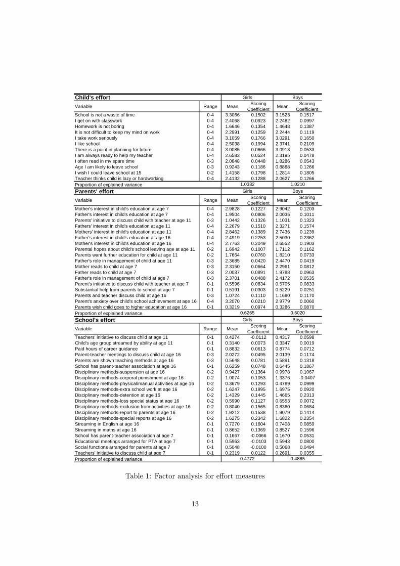
Table 1 contains the scoring coefficients for the child’s, the parents’ and the

school’s effort indicators obtained from the factor analyses performed separately

for boys and for girls. The scoring factors are the weights actually entering the

construction of the effort indicators. To reduce the loss of information due to

non-response, we impute the factor scores for the cases with missing data in

some of the originally observed variables on which the indices are based. The

imputation method is such that the new variable created includes predictions

for the missing values based on the best available subset of otherwise present

data. We have imputed 7%, 13.1% and 6.9% of the child’s, the parents’ and

the school’s effort information, respectively.

The child’s effort indicators used to construct the child’s effort measure eCiare the child’s answers (at age 16) to questions about her attitude towards

school, wishes and expectations about school leaving age, and the frequency of

reading (a higher value denotes higher effort).12 This information is comple-

mented by the teacher’s assessment of the child’s effort when the individuals

are 16 (the last row in the first part of Table 1). Columns 3 and 5 of Table

1 provide the scoring coefficients for each of the variables reflecting the effort

indicators, namely the weights actually entering the construction of the effort

indices. For the children the variable with the highest scoring coefficient is

whether the child likes school or not.13

The parents’ effort measure ePi is produced using both parents’ interest in

the child, their initiative to discuss the child’s progress in school, the father’s

role in the management of the child, the parents’ wishes and anxiety over the

child’s school achievement, and how often both parents read to their children.12The exact description of how we have constructed these and all the other variables is

in an Appendix available on request or at www.le.ac.uk/economics/gdf4/curres.htm. Thisappendix also reports the factor loadings.13The proportion of explained variance is approximately 1. This provides very strong

evidence that selecting only one factor is the most appropriate decision.

12

Child's effortVariable Range Mean Scoring

Coefficient Mean ScoringCoefficient

School is not a waste of time 0-4 3.3066 0.1502 3.1523 0.1517I get on with classwork 0-4 2.4068 0.0923 2.2482 0.0997Homework is not boring 0-4 1.6646 0.1354 1.4648 0.1387It is not difficult to keep my mind on work 0-4 2.2991 0.1259 2.2444 0.1119I take work seriously 0-4 3.1059 0.1766 3.0291 0.1650I like school 0-4 2.5038 0.1994 2.3741 0.2109There is a point in planning for future 0-4 3.0085 0.0666 3.0913 0.0533I am always ready to help my teacher 0-4 2.6583 0.0524 2.3195 0.0478I often read in my spare time 0-3 2.0848 0.0448 1.8286 0.0543Age I am likely to leave school 0-3 0.9243 0.1186 0.8868 0.1266I wish I could leave school at 15 0-2 1.4158 0.1798 1.2814 0.1805Teacher thinks child is lazy or hardworking 0-4 2.4132 0.1288 2.0627 0.1266Proportion of explained varianceParents' effortVariable Range Mean Scoring

Coefficient Mean ScoringCoefficient

Mother's interest in child's education at age 7 0-4 2.9828 0.1227 2.9042 0.1203Father's interest in child's education at age 7 0-4 1.9504 0.0806 2.0035 0.1011Parents' initiative to discuss child with teacher at age 11 0-3 1.0442 0.1326 1.1031 0.1323Fathers' interest in child's education at age 11 0-4 2.2679 0.1510 2.3271 0.1574Mothers' interest in child's education at age 11 0-4 2.8462 0.1389 2.7436 0.1239Father's interest in child's education at age 16 0-4 2.4919 0.2253 2.5030 0.2362Mother's interest in child's education at age 16 0-4 2.7763 0.2049 2.6552 0.1903Parental hopes about child's school leaving age at age 11 0-2 1.6942 0.1007 1.7112 0.1162Parents want further education for child at age 11 0-2 1.7664 0.0760 1.8210 0.0733Father's role in management of child at age 11 0-3 2.3685 0.0420 2.4470 0.0419Mother reads to child at age 7 0-3 2.3150 0.0664 2.2961 0.0812Father reads to child at age 7 0-3 2.0037 0.0891 1.9788 0.0963Father's role in management of child at age 7 0-3 2.3701 0.0488 2.4172 0.0535Parent's initiative to discuss child with teacher at age 7 0-1 0.5596 0.0834 0.5705 0.0833Substantial help from parents to school at age 7 0-1 0.5191 0.0303 0.5229 0.0251Parents and teacher discuss child at age 16 0-3 1.0724 0.1110 1.1680 0.1170Parent's anxiety over child's school achievement at age 16 0-4 3.2070 0.0210 2.9779 0.0060Parents wish child goes to higher education at age 16 0-1 0.3219 0.0974 0.3286 0.0870Proportion of explained varianceSchool's effortVariable Range Mean Scoring

Coefficient Mean ScoringCoefficient

Teachers' initiative to discuss child at age 11 0-1 0.4274 -0.0112 0.4317 0.0598Child's age group streamed by ability at age 11 0-1 0.3140 0.0073 0.3347 0.0019Paid hours of career guidance 0-1 0.8832 0.0613 0.8774 0.0712Parent-teacher meetings to discuss child at age 16 0-3 2.0272 0.0495 2.0139 0.1174Parents are shown teaching methods at age 16 0-3 0.5648 0.0781 0.5891 0.1318School has parent-teacher association at age 16 0-1 0.6259 0.0748 0.6445 0.1867Disciplinary methods-suspension at age 16 0-2 0.9427 0.1364 0.9978 0.1067Disciplinary methods-corporal punishment at age 16 0-2 1.0074 0.1053 1.3376 -0.0407Disciplinary methods-physical/manual activities at age 16 0-2 0.3679 0.1293 0.4789 0.0999Disciplinary methods-extra school work at age 16 0-2 1.6247 0.1995 1.6975 0.0920Disciplinary methods-detention at age 16 0-2 1.4329 0.1445 1.4665 0.2313Disciplinary methods-loss special status at age 16 0-2 0.5990 0.1127 0.6553 0.0072Disciplinary methods-exclusion from activities at age 16 0-2 0.8040 0.1565 0.8360 0.0684Disciplinary methods-report to parents at age 16 0-2 1.9212 0.1538 1.9079 0.1414Disciplinary methods-special reports at age 16 0-2 1.6275 0.2342 1.6822 0.2354Streaming in English at age 16 0-1 0.7270 0.1604 0.7408 0.0859Streaming in maths at age 16 0-1 0.8652 0.1369 0.8527 0.1596School has parent-teacher association at age 7 0-1 0.1667 -0.0066 0.1670 0.0531Educational meetings arranged for PTA at age 7 0-1 0.5963 -0.0103 0.5943 0.0800Social functions arranged for parents at age 7 0-1 0.5048 -0.0100 0.5068 0.0494Teachers' initiative to discuss child at age 7 0-1 0.2319 0.0122 0.2691 0.0355Proportion of explained variance

Girls Boys

0.4865

1.0210Boys

0.6020Boys

1.0332

0.4772

Girls

Girls

0.6265

Table 1: Factor analysis for effort measures

13

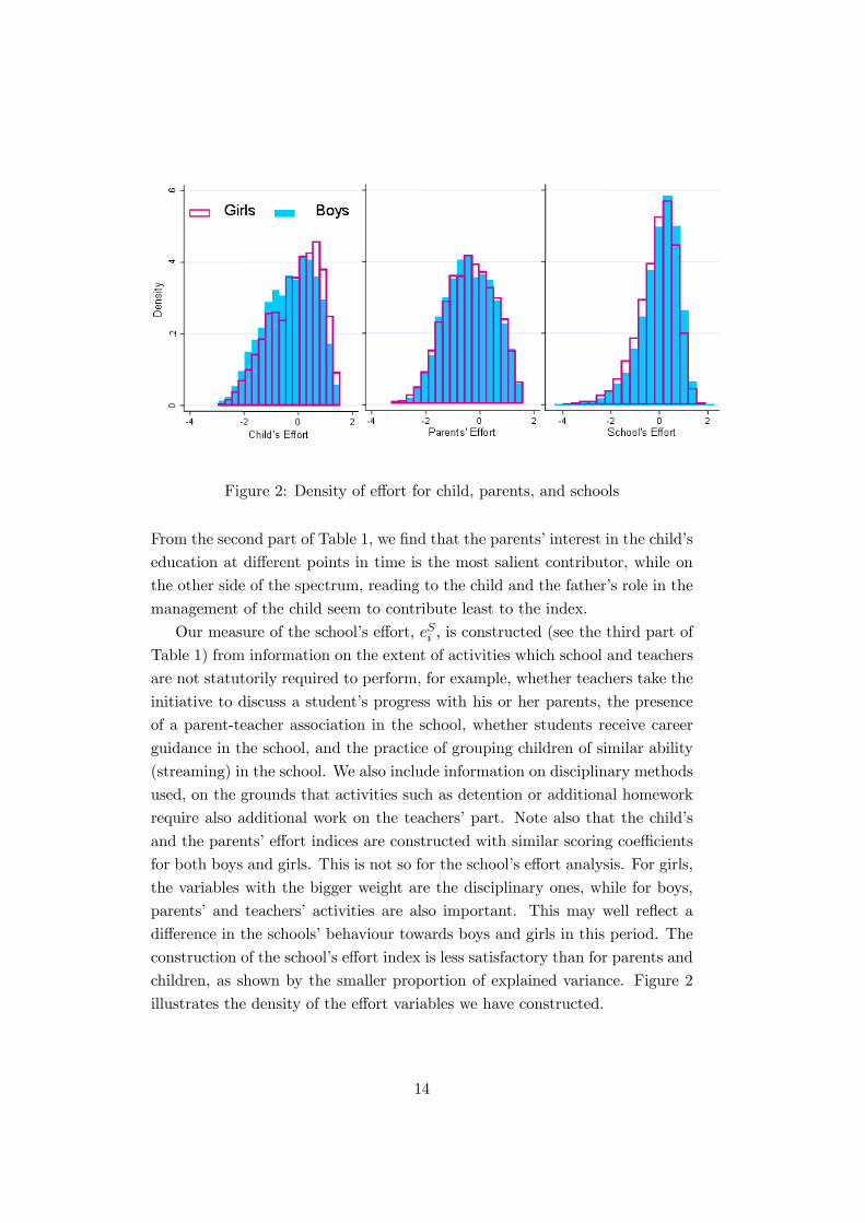
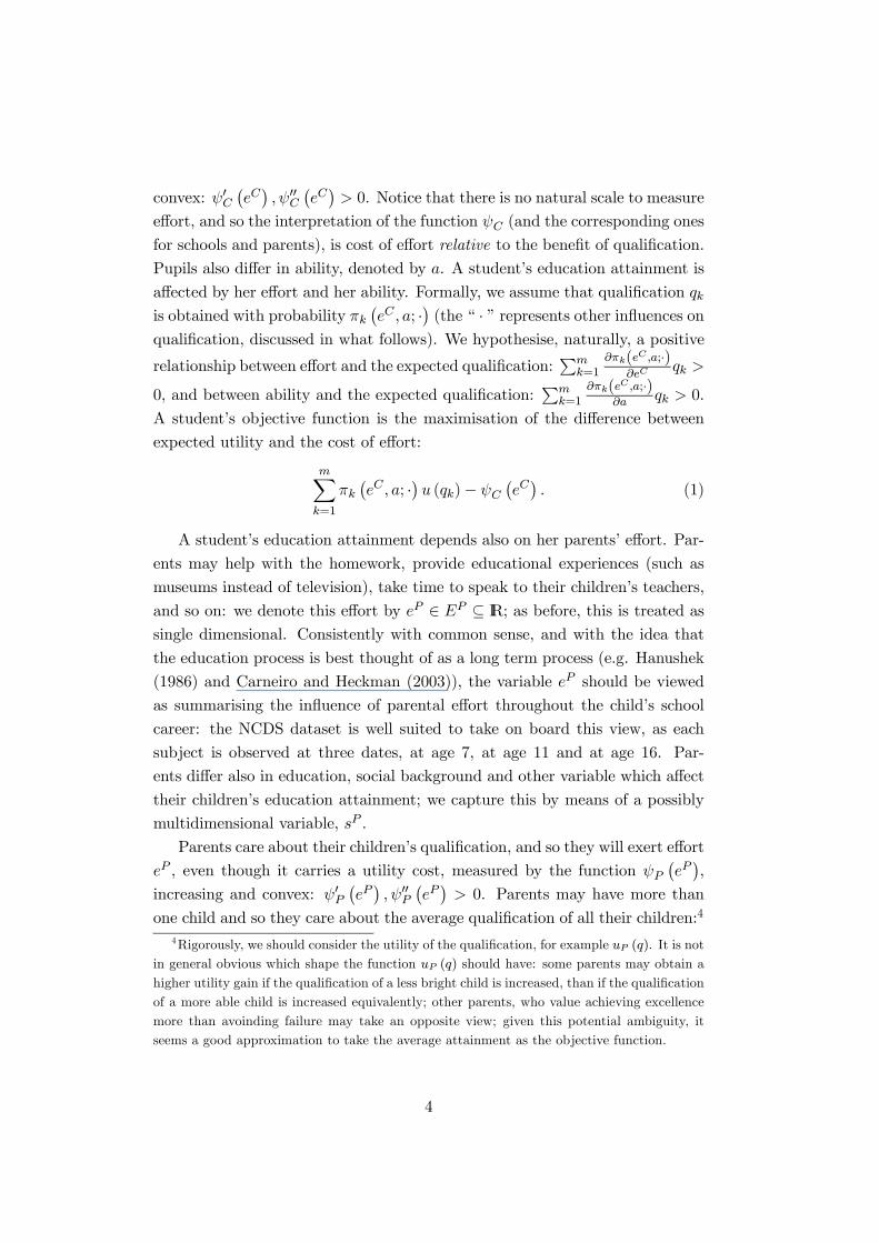
Figure 2: Density of effort for child, parents, and schools

From the second part of Table 1, we find that the parents’ interest in the child’s

education at different points in time is the most salient contributor, while on

the other side of the spectrum, reading to the child and the father’s role in the

management of the child seem to contribute least to the index.

Our measure of the school’s effort, eSi , is constructed (see the third part of

Table 1) from information on the extent of activities which school and teachers

are not statutorily required to perform, for example, whether teachers take the

initiative to discuss a student’s progress with his or her parents, the presence

of a parent-teacher association in the school, whether students receive career

guidance in the school, and the practice of grouping children of similar ability

(streaming) in the school. We also include information on disciplinary methods

used, on the grounds that activities such as detention or additional homework

require also additional work on the teachers’ part. Note also that the child’s

and the parents’ effort indices are constructed with similar scoring coefficients

for both boys and girls. This is not so for the school’s effort analysis. For girls,

the variables with the bigger weight are the disciplinary ones, while for boys,

parents’ and teachers’ activities are also important. This may well reflect a

difference in the schools’ behaviour towards boys and girls in this period. The

construction of the school’s effort index is less satisfactory than for parents and

children, as shown by the smaller proportion of explained variance. Figure 2

illustrates the density of the effort variables we have constructed.

14

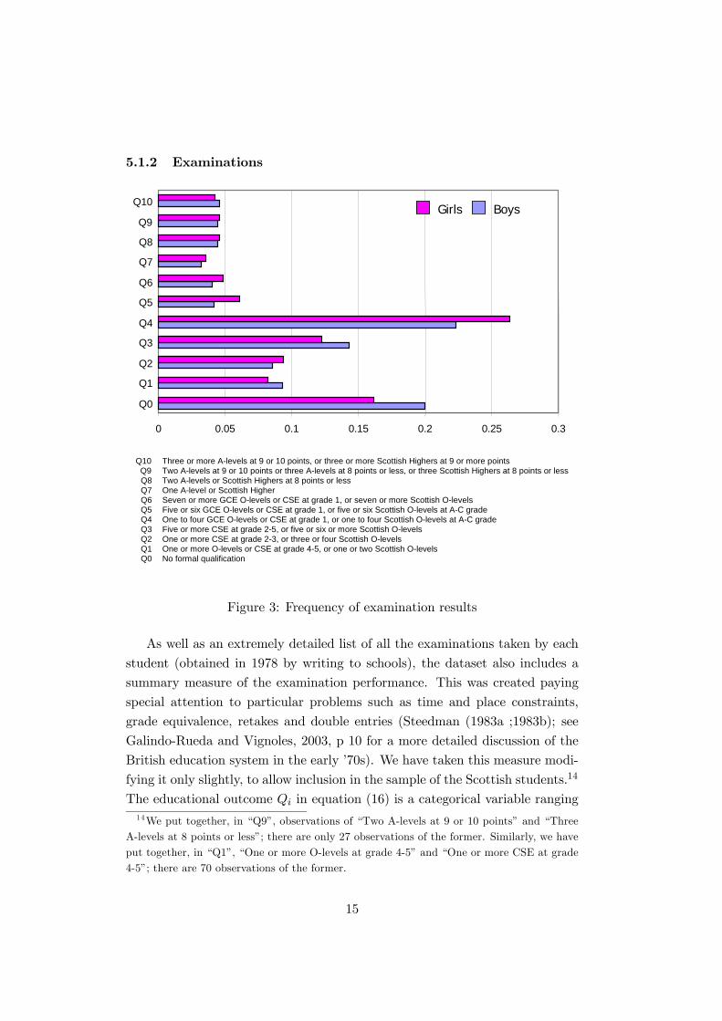
5.1.2 Examinations

Q10

Q9

Q8

Q7

Q6

Q5

Q4

Q3

Q2

Q1

Q0

0 0.05 0.1 0.15 0.2 0.25 0.3

Girls Boys

Q10 Three or more A-levels at 9 or 10 points, or three or more Scottish Highers at 9 or more pointsQ9 Two A-levels at 9 or 10 points or three A-levels at 8 points or less, or three Scottish Highers at 8 points or lessQ8 Two A-levels or Scottish Highers at 8 points or lessQ7 One A-level or Scottish HigherQ6 Seven or more GCE O-levels or CSE at grade 1, or seven or more Scottish O-levelsQ5 Five or six GCE O-levels or CSE at grade 1, or five or six Scottish O-levels at A-C gradeQ4 One to four GCE O-levels or CSE at grade 1, or one to four Scottish O-levels at A-C gradeQ3 Five or more CSE at grade 2-5, or five or six or more Scottish O-levelsQ2 One or more CSE at grade 2-3, or three or four Scottish O-levelsQ1 One or more O-levels or CSE at grade 4-5, or one or two Scottish O-levelsQ0 No formal qualification

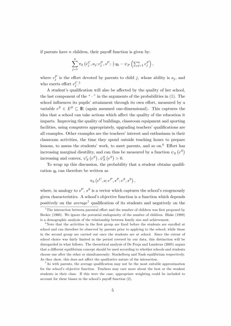
Figure 3: Frequency of examination results

As well as an extremely detailed list of all the examinations taken by each

student (obtained in 1978 by writing to schools), the dataset also includes a

summary measure of the examination performance. This was created paying

special attention to particular problems such as time and place constraints,

grade equivalence, retakes and double entries (Steedman (1983a ;1983b); see

Galindo-Rueda and Vignoles, 2003, p 10 for a more detailed discussion of the

British education system in the early ’70s). We have taken this measure modi-

fying it only slightly, to allow inclusion in the sample of the Scottish students.14

The educational outcome Qi in equation (16) is a categorical variable ranging14We put together, in “Q9”, observations of “Two A-levels at 9 or 10 points” and “Three

A-levels at 8 points or less”; there are only 27 observations of the former. Similarly, we haveput together, in “Q1”, “One or more O-levels at grade 4-5” and “One or more CSE at grade4-5”; there are 70 observations of the former.

15

from 0, indicating no formal qualification, to 10, reflecting 3 or more A-levels

at 9 to 10 points. Figure 3 shows the distribution of examination results for

boys and girls in the samples used. The proportion of boys that have at least

one A-level result is slightly higher, 17.37 against 16.66 for girls. The mode of

both distributions is “up to four O-levels or CSE with grade 1”.

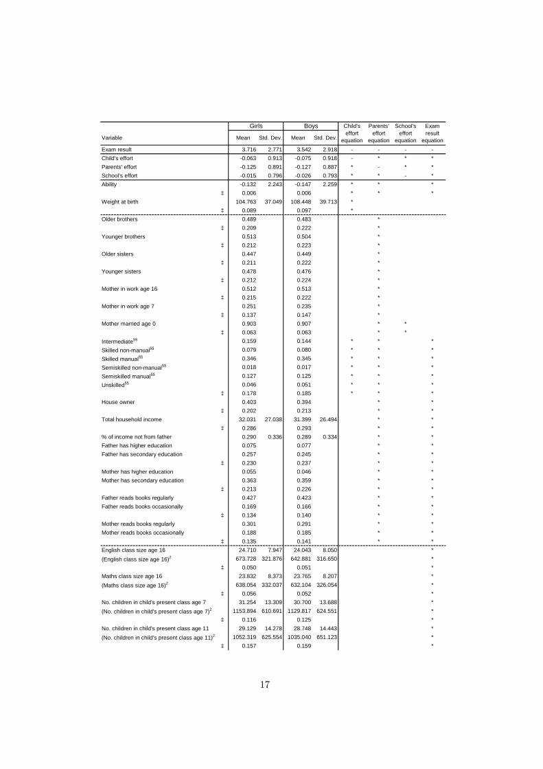
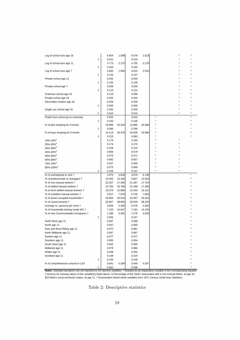
5.2 Explanatory variables

The summary statistics for the background explanatory variables are reported

in Table 2: individual characteristics first, then family characteristics, followed

by school, peer group and geographical variables.

The main individual characteristic is ability. This is measured at ages 7, 11,

and 16 by administered tests that are independent of educational qualifications.

At 7 there is information on arithmetic and reading scores, at 11 and 16 the

individuals were tested on their reading and mathematical ability, and at 11

they also completed a general ability test. Following the literature on cognitive

ability and students’ attainment, we combine the tests undertaken at the dif-

ferent points in time and on different subjects using the principal components

method (see, for example, Galindo-Rueda and Vignoles (2003)). We include

birth weight following some of the literature on lifetime attainments (Conley

et al. (2003); Fryer and Levitt (2002)).

The vector of family background variables includes the number of older

and younger brothers and sisters, and indicators of the mother’s position in the

labour market. Parental income is measured when the individuals were 16, and

the household socio-economic status is measured by the father’s (or the father

figure’s) social class at age 11.15 We have also included the percentage of total

income not earned by the father figure, and whether the household’s accom-

modation is owned by the household. Other variables are parental education

attainment and the frequency of reading of both parents, as distinct from the

variable measuring the frequency of parents reading to their children, which

enters the measure of parental effort.

The school characteristics we use are its size, measured by the log of the

number of pupils, and its type: state or private at ages 7, 11, and 16, and

single-sex, comprehensive, secondary modern or grammar at age 16. We also

include class size, and to capture possible non-linearities in class and school15We manipulated all income information using the procedure developed for this dataset

(Micklewright (1986)).

16

Variable Mean Std. Dev. Mean Std. Dev.

Exam result 3.716 2.771 3.542 2.918 - - - -Child's effort -0.063 0.913 -0.075 0.918 - * * *Parents' effort -0.125 0.891 -0.127 0.887 * - * *School's effort -0.015 0.796 -0.026 0.793 * * - *Ability -0.132 2.243 -0.147 2.259 * * *

‡ 0.006 0.006 * * *Weight at birth 104.763 37.049 108.448 39.713 *

‡ 0.089 0.097 *Older brothers 0.489 0.483 *

‡ 0.209 0.222 *Younger brothers 0.513 0.504 *

‡ 0.212 0.223 *Older sisters 0.447 0.449 *

‡ 0.211 0.222 *Younger sisters 0.478 0.476 *

‡ 0.212 0.224 *Mother in work age 16 0.512 0.513 *

‡ 0.215 0.222 *Mother in work age 7 0.251 0.235 *

‡ 0.137 0.147 *Mother married age 0 0.903 0.907 * *

‡ 0.063 0.063 * *Intermediate§§ 0.159 0.144 * * *Skilled non-manual§§ 0.079 0.080 * * *Skilled manual§§ 0.346 0.345 * * *Semiskilled non-manual§§ 0.018 0.017 * * *Semiskilled manual§§ 0.127 0.125 * * *Unskilled§§ 0.046 0.051 * * *

‡ 0.178 0.185 * * *House owner 0.403 0.394 * *

‡ 0.202 0.213 * *Total household income 32.031 27.038 31.399 26.494 * *

‡ 0.286 0.293 * *% of income not from father 0.290 0.336 0.289 0.334 * *Father has higher education 0.075 0.077 * *Father has secondary education 0.257 0.245 * *

‡ 0.230 0.237 * *Mother has higher education 0.055 0.046 * *Mother has secondary education 0.363 0.359 * *

‡ 0.213 0.226 * *Father reads books regularly 0.427 0.423 * *Father reads books occasionally 0.169 0.166 * *

‡ 0.134 0.140 * *Mother reads books regularly 0.301 0.291 * *Mother reads books occasionally 0.188 0.185 * *

‡ 0.135 0.141 * *English class size age 16 24.710 7.947 24.043 8.050 *(English class size age 16)2 673.728 321.876 642.881 316.650 *

‡ 0.050 0.051 *Maths class size age 16 23.832 8.373 23.765 8.207 *(Maths class size age 16)2 638.054 332.037 632.104 326.054 *

‡ 0.056 0.052 *No. children in child's present class age 7 31.254 13.309 30.700 13.688 *(No. children in child's present class age 7)2 1153.894 610.691 1129.817 624.551 *

‡ 0.116 0.125 *No. children in child's present class age 11 29.129 14.278 28.748 14.443 *(No. children in child's present class age 11)2 1052.319 625.554 1035.040 651.123 *

‡ 0.157 0.159 *

Girls Boys Child'seffort

equation

Parents'effort

equation

School'seffort

equation

Examresult

equation

17

Log of school size age 16 6.554 1.098 6.578 1.023 * *‡ 0.021 0.016 * *

Log of school size age 11 4.773 2.175 4.755 2.179 * *‡ 0.163 0.164 * *

Log of school size age 7 4.650 1.994 4.615 2.010 * *‡ 0.143 0.147 * *

Private school age 11 0.032 0.034 * *‡ 0.135 0.139 * *

Private school age 7 0.029 0.026 * *‡ 0.113 0.122 * *

Grammar school age 16 0.123 0.098 * *Private school age 16 0.034 0.040 * *Secondary modern age 16 0.204 0.205 * *

‡ 0.000 0.000 * *Single sex school age 16 0.262 0.235 * *

‡ 0.012 0.010 * *Pupils from school go to university 0.534 0.542 * *

‡ 0.163 0.146 * *% of girls studying for O-levels 24.958 33.225 13.895 26.088 * *

‡ 0.065 0.295 * *% of boys studying for O-levels 14.119 26.478 24.928 33.994 * *

‡ 0.313 0.063 * *10%-19%§ 0.174 0.163 * *20%-29%§ 0.174 0.170 * *30%-39%§ 0.109 0.123 * *40%-49%§ 0.069 0.079 * *50%-59%§ 0.075 0.071 * *60%-69%§ 0.062 0.057 * *70%-79%§ 0.027 0.035 * *80%-100%§ 0.073 0.069 * *

‡ 0.155 0.137 * *% of unemployed or sick † 3.975 5.818 3.879 6.138 *% of professionals or managers † 10.493 13.183 9.827 12.943 *% of non-manual workers † 22.527 17.300 21.287 17.724 *% of skilled manual workers † 22.763 16.796 21.446 17.284 *% of semi-skilled manual workers † 15.079 12.866 14.434 13.131 *% of unskilled manual workers † 5.917 7.676 5.746 7.604 *% of owner occupied households † 35.854 35.914 33.397 35.262 *% of council tenants † 30.667 38.803 29.006 38.229 *Average no. persons per room † 0.506 0.290 0.476 0.300 *% of households lacking inside WC † 7.133 14.047 7.191 14.155 *% of new Commonwealth immigrants † 1.286 5.091 1.278 5.033 *

‡ 0.205 0.247 *North West age 11 0.097 0.088 *North age 11 0.057 0.060 *East and West Riding age 11 0.072 0.081 *North Midlands age 11 0.067 0.067 *Eastern age 11 0.077 0.077 *Southern age 11 0.055 0.054 *South West age 11 0.062 0.056 *Midlands age 11 0.079 0.080 *Wales age 11 0.048 0.054 *Scotland age 11 0.108 0.104 *

‡ 0.134 0.139 *% of comprehensive schools in LEA 0.641 0.299 0.649 0.297 *

‡ 0.061 0.058 *Notes: Standard deviations are not reported for 0/1 dummy variables. * Included as an explanatory variable in the corresponding equation‡ Dummy for missing values of the variable(s) listed above. § Percentage of the child's classmates with a non-manual father, at age 16.§§ Father's socio-economic status, at age 11. † Enumeration district-level variables from 1971 Census Small Area Statistics

Table 2: Descriptive statistics

18

size (implying, for example that an increase in size may be a good thing for

small size, and a bad thing for larger size) we include the square of the size.

An important influence on the school’s quality are the characteristics of the

students in the school, that is the “peer group effect”.16 To capture it, we

consider both academic and social indicators. The former are the percentage

of boys and girls in the school attended at age 16 who are studying for O-

levels and the proportion who subsequently enrolled into a higher education

course (both indicate a more “academic” peer group). The social peer group

is captured by the proportion of children in the individual’s school class whose

father has a non-manual occupation.

The last rows of the Table report some geographical characteristics. As

well as regional dummies, we include the proportion of comprehensive schools

in the area, and some social indicators of the enumeration district (this is a

small geographical area comprising around 200 households) where the child

was living at age 16. These variables are taken from the 1971 census, and

correspond to those used by Dearden et al. (2002).

The last four columns in the Table illustrate the model specification we

have chosen: an asterisk in a column indicates that the variable in the row

was used as a regressor for the equation indicated by that column. Dummies

for missing values are used for each of the other variables to capture possible

non-randomness in non-response: these are the unnamed variables in the table,

after each variable or group of variables; for example the 0.089 in the line below

“Weight at birth” indicates that 8.9% of the data in the sample did not report

the value of this variable. All estimations include these dummy variables, but

we do not report their coefficients or standard errors in the results to make the

interpretation and the reading of the tables easier.

6 Results

Our theoretical foundation is that the effort of the three agents is simultane-

ously determined at the Nash equilibrium. Econometrically, the effort variables

should be endogenous. To ascertain this, we perform the DWH test described

in Section 4 on the parameters of equation (15). We can reject, at conven-16This is a well documented phenomenon; see Moreland and Levine (1992) for a survey

from a psychology/education viewpoint, Summers and Wolfe (1977), Henderson et al. (1978)for early economic empirical studies, and Epple et al. (2002) and Zimmer and Toma (2000)for more recent ones. The theoretical analyses of Arnott and Rowse (1987) and de Bartolome(1990) were among the first to take the peer group effect explicitly into account.

19

tional significance levels, the null hypothesis that the residuals of the effort

equations do not affect examination results,17 and we therefore conclude that

educational attainment and the effort levels exerted by children, their parents

and their school are indeed simultaneously determined, as posited by the the-

oretical model.

All the results are reported separately for the samples of girls and boys. We

have tested, and found support for, the hypothesis that girls and boys differ

significantly. We have done so by estimating a more general specification of the

entire model with a gender dummy interacting with each of the explanatory

variables, and testing the joint statistical significance of the parameters of these

interaction terms in the educational attainment equation, using a log-likelihood

ratio test.18

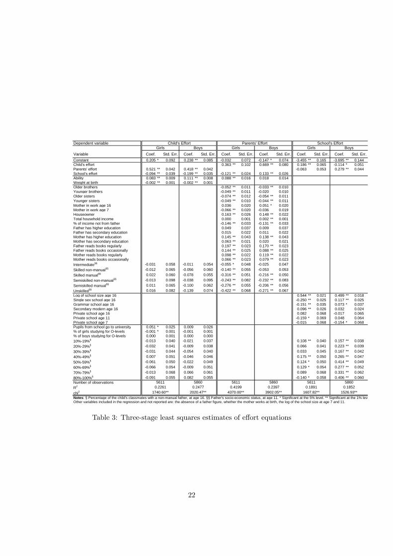
In Table 3 we report the results for our three-stage least squares estimates

of equations (9)-(11).19 In each of the three effort equations, the effort level

exerted by the other two groups of agents is significant, with the exception of

parental effort on the school effort for girls. This confirms our assumption of

simultaneous endogenous determination of effort levels as a Nash equilibrium.

Also note that a 0 coefficient does not necessary falsify the Nash equilibrium

hypothesis, because the intersection of the relevant best reply functions could

happen close to a stationary point of one of them (as, for example, in point

E1 in panel (a) in Figure 1). The table suggests that parental and the child’s

efforts are strategic complements: by exerting more effort, parents induce their

child to exert more effort, and, vice versa, parents respond positively to their

children exerting more effort. In other words, there is a “multiplier” effect,

suggesting, for example, that policies aimed at affecting directly the effort ex-

erted by children and parents may prove very effective. On the other hand, the

role of the school effort is less clear-cut: it affects negatively the effort exerted

by children and by girls’ parents, and positively the effort of boys’ parents.

Conversely, schools respond positively to girls’ effort, and negatively to boys’,17The test statistics of the likelihood-ratio tests of the null hypothesis are χ2 (3) = 7.86

(p-value 0.0491) for the sample of girls, χ2 (3) = 14.49 (p-value 0.0023) for the sample of boys,and χ2 (3) = 21.71 (p-value 0.0001) for the combined sample of girls and boys.18The test statistic of this likelihood-ratio test is χ2 (88) = 172.89 (p-value 0.0000). We

prefer to report separate samples, rather than the more general model with the interactionterms because its very large number of regressors would make the interpretation of coefficientsvery difficult.19We have tried several alternative specifications, and we present here only the most parsi-

monious, having tested at various stages for linear restrictions on non-significant coefficients.Other intermediate results and the data to obtain them are available on request.

20

but positively to boys’ parents’ effort. Anecdotal evidence does confirm the

possibility of differential attitude of schools and parents towards boys and girls

in the ’60s and early ’70s.

The striking feature of the children’s effort equation is the paucity of statis-

tically significant explanatory variables: only the other effort levels and their

own ability and birth weight seem to affect their effort. Clearly, our results are

tentative, constrained by the limitations of the dataset, but a possible interpre-

tation for this finding is that children from different backgrounds or in different

peer groups do not differ significantly in their propensity to exert effort. If

confirmed by more targeted studies, this may have policy implications for the

type of incentives to provide to pupils in schools.

The parents’ effort equation indicates that the presence of (older or younger)

siblings reduces parental effort. This is an interesting result, which also indi-

cates that the variables we have used to measure effort do indeed capture rele-

vant features of parental effort: theoretical considerations suggest that parents

face a trade-off between the number of their children and the attention each

of them receive (Becker (1960); Hanushek (1992)). Social class also appears

relevant. Parental taste for education, as reflected by their education and the

frequency of their reading, does positively influence their own effort. There

is also some indication that the mother’s position in the labour market may

have some effect on parental effort: the effect of the mother being in work is

rather ambiguous, but the percentage of household income not earned by the

father figure has a clear negative influence on parents’ effort. This confirms

the intuition that parents’ effort is not fully captured by their socio-economic

status. Household income, on the other hand, affects parental effort only for

boys.

The school’s effort is higher in larger schools, for both boys and girls. The

effects of school type variables are generally stronger for girls than for boys. It

is interesting to note the different effect of the “single-sex” variable in the two

subsamples: it suggests that girls’ only schools exert less effort, and boys’ only

schools more effort than co-educational schools; this is in line with our per-

ception of the British educational system at the time. Note that for younger

children (age 7 and 11), private schools exert effort level either not significantly

different or lower than state schools. At age 16, their effort level is not signifi-

cantly different from the base school type, the state comprehensive. The effect

of the peer group is statistically significant, especially for boys: schools work

harder which have a larger proportion of children from higher socio-economic

21

Dependent variable

Variable Coef. Std. Err. Coef. Std. Err. Coef. Std. Err. Coef. Std. Err. Coef. Std. Err. Coef. Std. Err.Constant 0.205 * 0.092 0.238 ** 0.085 -0.032 0.072 -0.147 * 0.074 -3.455 ** 0.165 -3.695 ** 0.144Child's effort 0.363 ** 0.102 0.669 ** 0.080 0.186 ** 0.065 -0.114 * 0.051Parents' effort 0.521 ** 0.042 0.418 ** 0.042 -0.063 0.053 0.279 ** 0.044School's effort -0.094 ** 0.039 -0.199 ** 0.035 -0.121 ** 0.024 0.133 ** 0.026Ability 0.083 ** 0.009 0.111 ** 0.008 0.088 ** 0.016 0.018 0.014Weight at birth -0.002 ** 0.001 -0.002 ** 0.001Older brothers -0.052 ** 0.011 -0.033 ** 0.010Younger brothers -0.049 ** 0.011 -0.020 0.010Older sisters -0.074 ** 0.012 -0.054 ** 0.011Younger sisters -0.049 ** 0.010 -0.044 ** 0.011Mother in work age 16 0.036 0.020 0.051 * 0.020Mother in work age 7 -0.066 ** 0.020 -0.036 0.019Houseowner 0.163 ** 0.026 0.148 ** 0.022Total household income 0.000 0.001 0.002 ** 0.001% of income not from father -0.146 ** 0.033 -0.131 ** 0.033Father has higher education 0.049 0.037 0.009 0.037Father has secondary education 0.015 0.022 0.011 0.022Mother has higher education 0.145 ** 0.043 0.138 ** 0.043Mother has secondary education 0.063 ** 0.021 0.020 0.021Father reads books regularly 0.197 ** 0.023 0.170 ** 0.023Father reads books occasionally 0.144 ** 0.025 0.088 ** 0.025Mother reads books regularly 0.098 ** 0.022 0.119 ** 0.022Mother reads books occasionally 0.066 ** 0.023 0.079 ** 0.023Intermediate§§ -0.031 0.058 -0.011 0.054 -0.055 * 0.048 -0.025 0.047Skilled non-manual§§ -0.012 0.065 -0.056 0.060 -0.140 ** 0.055 -0.053 0.053Skilled manual§§ 0.022 0.060 -0.078 0.055 -0.316 ** 0.051 -0.216 ** 0.050Semiskilled non-manual§§ -0.013 0.098 -0.038 0.095 -0.243 ** 0.082 -0.232 ** 0.083Semiskilled manual§§ 0.011 0.065 -0.100 0.062 -0.276 ** 0.055 -0.206 ** 0.056Unskilled§§ 0.016 0.082 -0.139 0.074 -0.422 ** 0.068 -0.271 ** 0.067Log of school size age 16 0.544 ** 0.021 0.499 ** 0.018Single sex school age 16 -0.250 ** 0.025 0.117 ** 0.025Grammar school age 16 -0.151 ** 0.035 0.073 * 0.037Secondary modern age 16 0.096 ** 0.026 0.032 0.024Private school age 16 0.082 0.068 -0.017 0.065Private school age 11 -0.159 * 0.069 0.048 0.064Private school age 7 -0.015 0.068 -0.154 * 0.068Pupils from school go to university 0.051 * 0.025 0.009 0.026% of girls studying for O-levels -0.001 * 0.001 -0.001 0.001% of boys studying for O-levels 0.000 0.001 0.000 0.00010%-19%§ -0.013 0.040 -0.021 0.037 0.108 ** 0.040 0.157 ** 0.03820%-29%§ -0.032 0.041 -0.009 0.038 0.066 0.041 0.223 ** 0.03930%-39%§ -0.031 0.044 -0.054 0.040 0.033 0.045 0.167 ** 0.04240%-49%§ 0.007 0.051 -0.046 0.046 0.175 ** 0.050 0.265 ** 0.04750%-59%§ -0.061 0.050 -0.022 0.049 0.124 * 0.050 0.414 ** 0.04960%-69%§ -0.066 0.054 -0.009 0.051 0.129 * 0.054 0.277 ** 0.05270%-79%§ -0.013 0.068 0.066 0.061 0.089 0.068 0.331 ** 0.06280%-100%§ -0.091 0.055 0.082 0.055 -0.140 * 0.058 0.406 ** 0.060Number of observationsR2

chi2

Notes: § Percentage of the child's classmates with a non-manual father, at age 16. §§ Father's socio-economic status, at age 11. * Significant at the 5% level. ** Significant at the 1% leve

0.41992020.47**

0.24770.22611740.60**

Child's EffortGirls Boys Girls Boys

Parents' Effort School's EffortGirls Boys

Other variables included in the regression and not reported are: the absence of a father figure, whether the mother works at birth, the log of the school size at age 7 and 11.

5611 5860 5611 5611 586058600.2397 0.1891 0.1852

1526.93**1607.82**3902.05**4370.00**

Table 3: Three-stage least squares estimates of effort equations

22

groups.

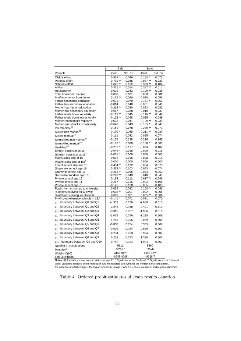
Table 4 presents the result of our ordered probit estimates. As it should,

effort strongly improves results. Ability also has, again as one would expect,

a strong independent positive effect on results. Family background variables,

such as the parents’ education, their taste for reading and their social class

have however a less definite effect than they had on effort, and they appear

to have a weaker influence than much of the literature suggests (Ermisch and

Francesconi (2001), Dearden et al. (2002)); for example, income is statistically

not significant. Whether the mother (the father) has higher education affect

positively girls’ (boys’) results, but otherwise parental education is not statisti-

cally significant. Book reading has, if anything, a negative effect on attainment,

and the social class is overall less significant than in the effort equation. A nat-

ural interpretation of these results is that family background influences school

examination’s results indirectly, via parental effort, rather than directly.

With regard to the variables describing the school, we find that being in a

private school has a direct positive effect for boys but not for girls; on the other

hand, for girls, a state grammar has a direct positive effect, while a secondary

modern has a direct negative effect. Girls in single-sex schools obtain, ceteris

paribus, a better qualification. School size matters only at age 16, and only

for girls, with a negative sign. These variables have the opposite sign in the

school’s effort equation: in Table 3, last columns, single-sex has a negative sign,

and the school size a positive sign. We have included several measures of class

size, at the three different ages, and their square, to account for possible non-

linearities: of these only the English class size at age 16, for girls, is statistically

significant.20 The academic peer group effect appears very strong: interestingly,

it operates within genders: girls are not influenced by boys and vice versa. This

makes sense, and we take it as a further indication that our model specification

is plausible.

We do not include in Table 4 the census variables, listed in Table 2. Among

them, only the percentage of unemployed or sick in the census enumeration

district are statistically significant for girls, and only the proportion of owner

occupied houses, the proportion of council tenants, and the average number

of persons per room are statistically significant for boys. These variables have20The estimated coefficients suggest that exam results improve with class size up to 29 and

decreases for class size larger than 30. Though the specific appealing value of the “optimal”class size may well be a fluke, it is interesting to note that the relationship between class sizeand achievement in this dataset has often the “wrong” sign (Levacic and Vignoles 2002)

23

Variable Coef. Std. Err. Coef. Std. Err.Child's effort 0.439 ** 0.046 0.164 * 0.073Parents' effort 0.739 ** 0.085 0.977 ** 0.033School's effort 1.076 ** 0.162 0.333 ** 0.104Ability 0.331 ** 0.014 0.357 ** 0.014Houseowner 0.001 0.043 -0.109 ** 0.038Total household income 0.000 0.001 0.000 0.001% of income not from father 0.179 ** 0.060 -0.028 0.058Father has higher education 0.071 0.070 0.161 * 0.063Father has secondary education -0.014 0.040 -0.001 0.040Mother has higher education 0.213 ** 0.080 -0.063 0.082Mother has secondary education -0.067 0.038 -0.010 0.037Father reads books regularly -0.119 ** 0.045 -0.146 ** 0.042Father reads books occasionally -0.122 ** 0.048 -0.025 0.048Mother reads books regularly -0.023 0.041 -0.109 ** 0.039Mother reads books occasionally -0.048 0.043 -0.105 * 0.043Intermediate§§ -0.151 0.078 -0.230 ** 0.073Skilled non-manual§§ -0.190 * 0.088 -0.211 ** 0.080Skilled manual§§ -0.111 0.082 -0.065 0.074Semiskilled non-manual§§ -0.155 0.138 -0.226 0.143Semiskilled manual§§ -0.187 * 0.089 -0.180 * 0.083Unskilled§§ -0.232 * 0.117 -0.093 0.102English class size at 16 0.046 * 0.018 0.000 0.018(English class size at 16)2 -0.001 * 0.000 0.000 0.000Maths class size at 16 0.001 0.016 0.008 0.016(Maths class size at 16)2 0.000 0.000 0.000 0.000Log of school size age 16 -0.434 ** 0.102 -0.084 0.070Single sex school age 16 0.353 ** 0.103 -0.093 0.074Grammar school age 16 0.211 ** 0.066 0.083 0.063Secondary modern age 16 -0.223 ** 0.049 0.018 0.045Private school age 16 0.193 0.112 0.617 ** 0.096Private school age 11 0.217 0.115 -0.002 0.105Private school age 7 -0.125 0.120 -0.055 0.103Pupils from school go to university 0.035 0.042 0.108 ** 0.041% of girls studying for O-levels 0.005 ** 0.001 -0.002 0.001% of boys studying for O-levels 0.000 0.001 0.005 ** 0.001% of comprehensive schools in LEA -0.141 * 0.071 -0.071 0.070µ1 : boundary between Q0 and Q1 -4.352 0.759 -2.956 0.610µ2 : boundary between Q1 and Q2 -3.843 0.758 -2.421 0.610µ3 : boundary between Q2 and Q3 -3.315 0.757 -1.966 0.610µ4 : boundary between Q3 and Q4 -2.678 0.756 -1.235 0.609µ5 : boundary between Q4 and Q5 -1.248 0.755 0.059 0.608µ6 : boundary between Q5 and Q6 -0.850 0.754 0.355 0.607µ7 : boundary between Q6 and Q7 -0.509 0.754 0.660 0.607µ8 : boundary between Q7 and Q8 -0.234 0.753 0.924 0.607µ9 : boundary between Q8 and Q9 0.202 0.753 1.338 0.607µ10 : boundary between Q9 and Q10 0.782 0.754 1.904 0.607Number of observationsPseudo R2

Wald chi2(90)Log-LikelihoodNotes: §§ Father's socio-economic status, at age 11. * Significant at the 5% level. ** Significant at the 1% level.Other variables included in the regression and not reported are: whether the mother is married at birth,the absence of a father figure, the log of school size at age 7 and 11, census variables, and regional dummies.

0.27444192.97**-9226.7-8945.4208

4166.01**0.2677

Girls Boys

5611 5860

Table 4: Ordered probit estimates of exam results equation

24

Child'seffort

Parents'effort

School'seffort

Child'seffort

Parents'effort

School'seffort

Q0 -0.028 -0.047 -0.069 -0.016 -0.095 -0.033Q1 -0.037 -0.063 -0.091 -0.018 -0.107 -0.037Q2 -0.054 -0.091 -0.132 -0.018 -0.105 -0.036Q3 -0.051 -0.086 -0.125 -0.014 -0.082 -0.028Q4 0.084 0.141 0.206 0.039 0.230 0.078Q5 0.037 0.062 0.090 0.010 0.057 0.019Q6 0.022 0.038 0.055 0.007 0.043 0.015Q7 0.012 0.020 0.029 0.004 0.025 0.009Q8 0.010 0.017 0.025 0.004 0.022 0.007Q9 0.004 0.007 0.011 0.002 0.010 0.004Q10 0.001 0.002 0.002 0.000 0.002 0.001

Girls Boys

Table 5: Marginal effects

a negative effect on examination results. With regard to regional dummies

(at age 11), “south” and “midlands” are positively significant for girls, and

“north”, “east and west riding” and “Scotland” for boys.21

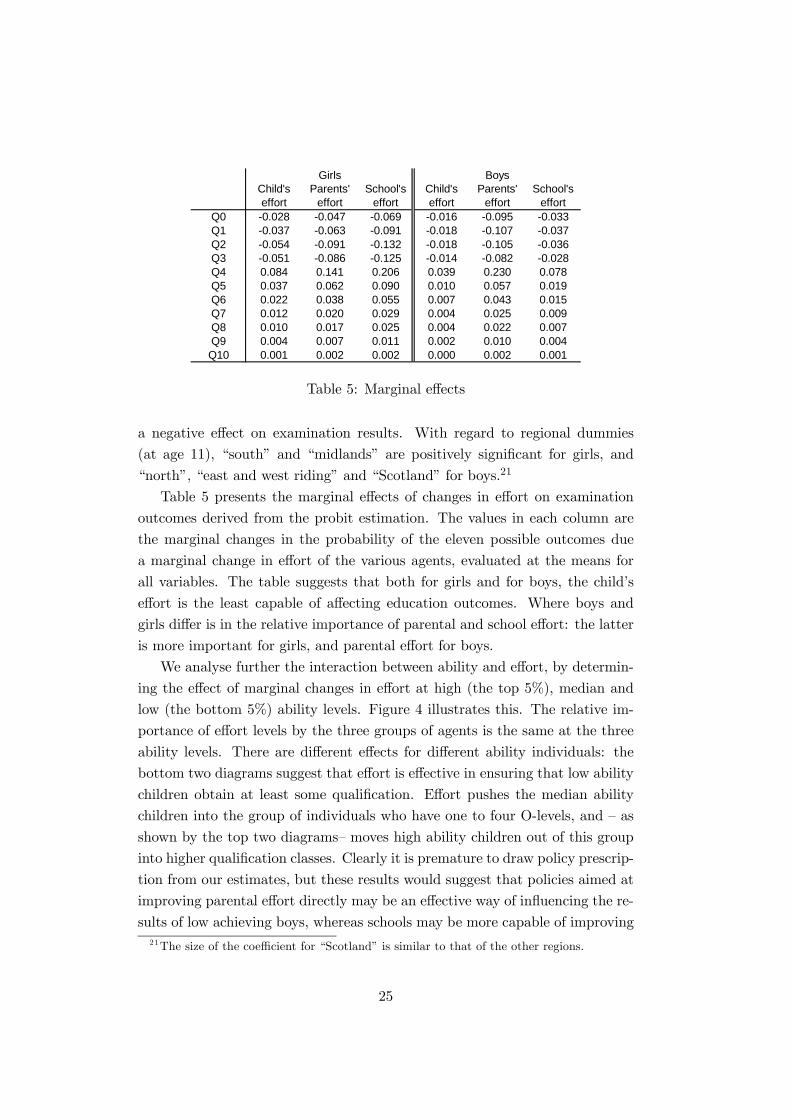
Table 5 presents the marginal effects of changes in effort on examination

outcomes derived from the probit estimation. The values in each column are

the marginal changes in the probability of the eleven possible outcomes due

a marginal change in effort of the various agents, evaluated at the means for

all variables. The table suggests that both for girls and for boys, the child’s

effort is the least capable of affecting education outcomes. Where boys and

girls differ is in the relative importance of parental and school effort: the latter

is more important for girls, and parental effort for boys.

We analyse further the interaction between ability and effort, by determin-

ing the effect of marginal changes in effort at high (the top 5%), median and

low (the bottom 5%) ability levels. Figure 4 illustrates this. The relative im-

portance of effort levels by the three groups of agents is the same at the three

ability levels. There are different effects for different ability individuals: the

bottom two diagrams suggest that effort is effective in ensuring that low ability

children obtain at least some qualification. Effort pushes the median ability

children into the group of individuals who have one to four O-levels, and — as

shown by the top two diagrams— moves high ability children out of this group

into higher qualification classes. Clearly it is premature to draw policy prescrip-

tion from our estimates, but these results would suggest that policies aimed at

improving parental effort directly may be an effective way of influencing the re-

sults of low achieving boys, whereas schools may be more capable of improving21The size of the coefficient for “Scotland” is similar to that of the other regions.

25

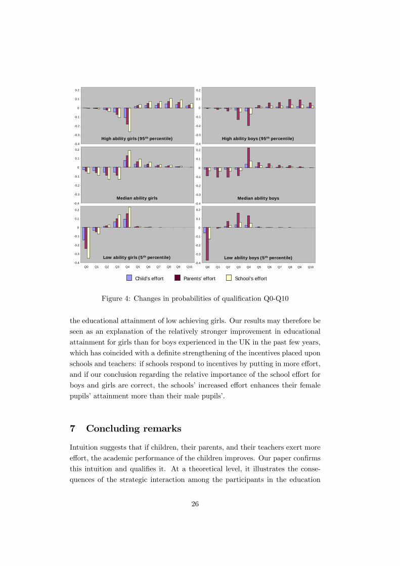
Child’s effort Parents’ effort School’s effort

-0.4

-0.3

-0.2

-0.1

0

0.1

0.2

-0.4

-0.3

-0.2

-0.1

0

0.1

0.2

-0.4

-0.3

-0.2

-0.1

0

0.1

0.2

-0.4

-0.3

-0.2

-0.1

0

0.1

0.2

Q0 Q1 Q2 Q3 Q4 Q5 Q6 Q7 Q8 Q9 Q10

-0.4

-0.3

-0.2

-0.1

0

0.1

0.2

-0.4

-0.3

-0.2

-0.1

0

0.1

0.2

Q0 Q1 Q2 Q3 Q4 Q5 Q6 Q7 Q8 Q9 Q10

High ability girls (95th percentile) High ability boys (95th percentile)

Median ability girls Median ability boys

Low ability girls (5th percentile) Low ability boys (5th percentile)

Figure 4: Changes in probabilities of qualification Q0-Q10

the educational attainment of low achieving girls. Our results may therefore be

seen as an explanation of the relatively stronger improvement in educational

attainment for girls than for boys experienced in the UK in the past few years,

which has coincided with a definite strengthening of the incentives placed upon

schools and teachers: if schools respond to incentives by putting in more effort,

and if our conclusion regarding the relative importance of the school effort for

boys and girls are correct, the schools’ increased effort enhances their female

pupils’ attainment more than their male pupils’.

7 Concluding remarks

Intuition suggests that if children, their parents, and their teachers exert more

effort, the academic performance of the children improves. Our paper confirms

this intuition and qualifies it. At a theoretical level, it illustrates the conse-

quences of the strategic interaction among the participants in the education

26

process: as a simple example shows, if effort levels are strategic substitutes,

then an increase in effort by the school may cause a reduction in effort by the

students. The model is tested empirically, with interesting results: for example

our finding that the school’s effort is more important for girls and the parents’

effort is more important for boys is not necessarily intuitive, even though it

can be rationalised ex-post. The same can be said of the findings that the chil-

dren’s effort seem to be less effective than both the parents’ and the school’s.

The next step is to understand what motivates children, their parents and their

teachers to exert effort. This can allow policy makers to design policies aimed

at stimulating effort: it may be easier and more effective to stimulate effort in

households with a low socioeconomic background, rather than wait for their

economic conditions to change.

The environment where schools operate has clearly changed radically, both

in term of the incentive system operating within schools and of the competitive

climate between schools. Nevertheless, understand which fundamental factors

affect the behaviour of the agents at the heart of the education production

process is important both to be able to evaluate the effects of the changing

environment and to predict the possible effects of proposed policy changes.

27

References

Arnott, R. and J. Rowse (1987). Peer group effects and educational attainment.Journal of Public Economics 32, 287—305.

Becker, G. S. (1960). An economic analysis of fertility. In Demographic and economicchange in developed countries. NBER - Princeton University Press, Princeton,no 11.

Becker, G. S. and N. Tomes (1976). Child endowments and the quantity and qualityof children. Journal of Political Economy 84, S143—62.

Blake, J. (1989). Familiy size and achievement. University of California Press, Berke-ley.

Bonesrønning, H. (1998). The importance of student effort in education production.empirical evidence from Norway. Department of Economics. Norwegian Univer-sity of Science and Technology.

Bonesrønning, H. (2004). The determinants of parental effort in education produc-tion: do parents respond to changes in class size? Economics of EducationReview 23, 1—9.

Bulow, J. I., J. D. Geanakoplos, and P. D. Klemperer (1985). Multimarket oligopoly:Strategic substitutes and complements. Journal of Political Economy 93, 488—511.

Cappelli, P. and K. Chauvin (1991). An interplant test of the efficiency wage hy-pothesis. Quarterly Journal of Economics 106, 769—787.

Carneiro, P. and J. Heckman (2003). Human capital policy. In J. Heckman andA. Krueger (Eds.), Inequality in America: What Role for Human Capital Poli-cies. MIT Press, Cambridge MA.

Conley, D., K. Strully, and N. G. Bennett (2003). A pound of flesh or just proxy?Using twin differences to estimate the effect of birth weight on life chances.Technical Report 9901, NBER Working Paper Series.

Connolly, S., J. Micklewright, and S. Nickell (1992). The occupational success ofyoung men who left school at sixteen. Oxford Economic Papers 44, 460—79.

Cooley, J. (2004). Equilibrium achievement under conformity effects. Departmentof Economics, Duke University.

CUSSRU (2000). National child development study composite file including selectedperinatal data and sweeps one to five, 1958-1991, 2nd edition. Technical report,City University Social Statistics Research Unit, National Birthday Trust Fund,National Children’s Bureau, City University Social Statistics Research Unit,Colchester, Essex.

Davidson, R. and J. G. MacKinnon (1993). Estimation and inference in economet-rics. Oxford University Press, New York.

28

de Bartolome, C. (1990). Equilibrium and inefficiency in a community model withpeer group effects. Journal of Political Economy 98, 110—133.

De Fraja, G. and P. Landeras (2005). Could do better: The effectiveness of incentivesand competition in schools. Journal of Public Economics forthcoming.

Dearden, L., C. Emmerson, C. Frayne, and C. Meghir (2003). The impact of financialincentives on education choice. Presented at the CEPR meeting, The Economicsof Education, Paris.

Dearden, L., J. Ferri, and C. Meghir (2002). The effect of school quality on educa-tional attainment and wages. Review of Economics and Statistics 84, 1—20.

Epple, D., R. E. Romano, and H. Sieg (2003). Peer effects financial aid and selectionof students to colleges and universities: An empirical analysis. Journal of AppliedEconometrics 18, 501—525.

Ermisch, J. and M. Francesconi (2001). Family matters: Impacts of family back-ground on educational attainments. Economica 68, 137—156.

Everitt, B. S. and G. Dunn (2001). Applied multivariate data analysis. Second edi-tion. Arnold, London.

Falk, A. and A. Ichino (2003). Clean evidence on peer pressure. European UniversityInstitute, Florence.

Fan, X. and M. Chen (2001). Parental involvement and students’ academic achieve-ment: A meta-analysis. Educational Psychology Review 13, 1—22.

Fryer, R. G. and S. D. Levitt (2004). Understanding the black-while test score gapin the first two years of school. Review of Economics and Statistics 86, 447—464.

Fudenberg, D. and J. Tirole (1991). Game theory. MIT Press, Cambridge, Massa-chusetts.

Galindo-Rueda, F. and A. Vignoles (2003). Class ridden or meritocratic? an eco-nomic analysis of recent changes in Britain. Technical Report 32, Centre for theEconomics of Education, London School of Economics.

Galizzi, M. and K. Lang (1998). Relative wages, wage growth, and quit behavior.Journal of Labor Economics 16, 367—391.

Hanushek, E. A. (1986). The economics of schooling: Production and efficiency inpublic schools. Journal of Economic Literature 23, 1141—77.

Hanushek, E. A. (1992). The trade-off between child quantity and quality. Journalof Political Economy 100, 84—117.

Harman, H. H. (1976). Modern factor analysis. Third edition. University of ChicagoPress, Chicago.

Henderson, V., P. Mieszkowski, and Y. Sauvageau (1978). Peer group effects ineducational production function. Journal of Public Economics 10, 97—106.

Holmstrom, B. R. and J. Tirole (1989). The theory of the firm. In R. Schmalenseeand R. D. Willig (Eds.), Handbook of industrial organization. Volume 1, pp.61—133. North-Holland, Amsterdam,.

29

Hoover-Dempsey, K. V., A. C. Battiato, J. M. T. Walker, R. P. Reed, J. M. De-Jong, and K. P. Jones (2001). Parental involvement in homework. EducationalPsychologist 36, 195—209.

Ichino, A. and G. Maggi (2000). Work environment and individual background: Ex-plaining regional shirking differentials in a large Italian firm. Quarterly Journalof Economics 115, 1057—1090.

Ichino, A. and R. Riphahn (2005). The effect of employment protection on workereffort: Absenteeism during and after probation. Journal of the European Eco-nomic Association 3, 120—143.

JCfLR (2001). National child development study and 1970 British cohort study(BCS70) follow-ups, 1999-2000. Technical report, Joint Centre for LongitudinalResearch, UK Data Archive, Colchester, Essex.

Levacic, R. C. and A. Vignoles (2002). Researching the links between school re-sources and student outcomes in the UK: A review of issues and evidence. Edu-cation Economics 10, 313—331.

Micklewright, J. (1986). A note on household income data in NCDS3. TechnicalReport 18, NCDS User Support Group, Social Statistics Research Unit, CityUniversity, London.

Micklewright, J. (1989). Choice at sixteen. Economica 56, 25—39.

Moreland, R. L. and J. M. Levine (1992). The composition of small groups. In E. J.Lawler, B. Markovsky, C. Ridgeway, and H. Walker (Eds.), Advances in groupprocesses, Vol 9, pp. 237—80. JAI Press, Greenwich, CT.

Natriello, G. and E. L. McDill (1986). Performance standards, student effort onhomework, and academic achievement. Sociology of Education 59, 18—31.

Shapiro, C. and J. E. Stiglitz (1984). Equilibrium unemployment as a worker disci-pline device. American Economic Review 74, 433—444.

Steedman, J. (1983a). Examination results in selective and non-selective schools:Findings from the National Child Development Study. National Children’s Bu-reau, London.

Steedman, J. (1983b). Examination results in selective and non-selective schools:Findings from the National Child Development Study. Volume 2 — Appendices.National Children’s Bureau, London.

Summers, A. A. and B. L. Wolfe (1977). Do schools make a difference? AmericanEconomic Review 67, 639—652.

Trautwein, U. and O. Köller (2003). The relationship between homework andachievement: Still much of a mystery. Educational Psychology Review 15, 115—45.

Zimmer, R. W. and E. F. Toma (2000). Peer effects in private and public schoolsacross countries. Journal of Policy Analysis and Management 19, 75—92.

30