Murtha, J. - Risk Analysis for the Oil Industry

A ComprehensiveStudy of Risk Management

Risk Analysis

for the Oil Industry

Risk Analysis

for the Oil Industry

A supplement to:

2 Risk Analysis

Jim Murtha, a registered petroleumengineer, presents seminars and trainingcourses and advises clients in buildingprobabilistic models in risk analysis anddecision making. He was elected toDistinguished Membership in SPE in1999, received the 1998 SPE Award inEconomics and Evaluation, and was1996-97 SPE Distinguished Lecturer inRisk and Decision Analysis. Since 1992,more than 2,500 professionals have takenhis classes. He has published Decisions

Involving Uncertainty - An @RISKTutorial for the Petroleum Industry. In25 years of academic experience, hechaired a math department, taught petro-leum engineering, served as academicdean, and co-authored two texts inmathematics and statistics. Jim has aPh.D. in mathematics from the Uni-versity of Wisconsin, an MS in petroleumand natural gas engineering from PennState and a BS in mathematics fromMarietta College. ◆

Risk Analysis:Table of Contents

When I was a struggling assistant professor ofmathematics, I yearned for more ideas, for wewere expected to write technical papers andsuggest wonderful projects to graduate students.Now I have no students and no one is countingmy publications. But, the ideas have beencoming. Indeed, I find myself, like anyone whoteaches classes to professionals, constantlystumbling on notions worth exploring.

The articles herein were generated during afew years and written mostly in about 6months. A couple of related papers found theirway into SPE meetings this year.

I thank the hundreds of people who listenedand challenged and suggested during classes.

I owe a lot to Susan Peterson, John Trahanand Red White, friends with whom I argue andbounce ideas around from time to time.

Most of all, these articles benefited by the carefulreading of one person,Wilton Adams,who has oftenassisted Susan and me in risk analysis classes.During the past year, he has been especially helpfulin reviewing every word of the papers I wrote forSPE and for this publication.Among his talents area well tuned ear and high standards for clarity.I wish to thank him for his generosity.

He also plays a mean keyboard, sings agood song and is a collaborator in a certainperiodic culinary activity.

You should be so lucky. ◆

Acknowledgements

▲

A Guide To Risk Analysis . . . . . . . . . . . . . . . . . . . . . . . . . 3Central Limit Theorem – Polls and Holes . . . . . . . . . . . 5Estimating Pay Thickness

From Seismic Data . . . . . . . . . . . . . . . . . . . . . . . . . . . 9Bayes’ Theorem – Pitfalls . . . . . . . . . . . . . . . . . . . . . . . . 12Decision Trees vs. Monte Carlo Simulation . . . . . . . . 14When Does Correlation Matter? . . . . . . . . . . . . . . . . . 19Beware of Risked Reserves . . . . . . . . . . . . . . . . . . . . 23

Table of Contents

▲

Biography

▲

RR

Risk Analysis 3

Risk Analysis:An Overview

Risk and decision analysis was born in the middleof the 20th century, about 50 years after some ofthe necessary statistics became formalized.Pearson defined standard deviation and skewnessin the late 1890s, and Galton introducedpercentiles in 1885.

The term Monte Carlo, as applied touncertainty analysis, was mentioned by Metropolisand Ulam: the Journal of the American StatisticalAssociation in 1940. D.B. Hertz published hisclassic Harvard Business Review article in 1964. Acouple of years later, Paul Newendorp beganteaching classes on petroleum explorationeconomics and risk analysis, out of which evolvedthe first edition of his text in 1975, the same yearas A.W. McCray and 2 years before R.E. Megillwrote their books on the subject.Ten years later,there was commercial software available to doMonte Carlo simulation.

During this 50-year period, decision analysis,featuring decision trees, also came of age. Raiffa’sclassic book appeared in 1968. By 1985, therewere several commercial applications of softwareon the market.

These developments, in many ways, paralleledthe development of petroleum engineering, withthe basics appearing in the 1930s, mature texts like

Craft and Hawkins appearing in the late 1950s, andreservoir simulation and other computer basedmethods emerging in the 1970s and 1980s.Similarly, reservoir characterization and geostatisticscame along in the second half of the 20th century.

Oddly, the oil and gas industry remainedskeptical about risk analysis throughout most of thisdevelopment period, usually limiting their accept-

ance to isolated departments within organizations.Managers were notoriously unwilling to embraceresults that presented probability distributions forreserves and net present value (NPV). Consultantsoffering services and software vendors know toowell these levels of resistance.

Now, finally, there seems to be broaderacceptance of probabilistic methods, although asI write, my SPE Technical Interest Group digestcontains strong negativism from traditionalistsabout probabilistic prices. Nonetheless, considerthese items:

• the three most recent and five out of the lastseven recipients of the SPE Economics andEvaluation award have been strong proponentsof risk analysis;

• whereas the index to the last edition of thePetroleum Engineers’ Handbook only had tworeferences to “risk,” the forthcoming editionwill feature an entire chapter on the topic;

• my first paper on Monte Carlo simulation waspresented at the Eastern Regional Meeting in1987 and summarily rejected by the editorialcommittees for not being of adequate generalinterest. (It was a case study dealing with theClinton formation, but the methods wereclearly generic and used popular material

balance notions). Ten years later, I publishedMonte Carlo Simulation, Its Status and Future inthe Distinguished Author series;

• the most popular SPE Applied TechnologyWorkshop focuses on probabilistic methods;

• SPE, SPEE and WPC are working ondefinitions that include probabilisticlanguage; and

A Guide To –

Risk Analysis

The oil and gas industry remained skeptical aboutrisk analysis throughout most of this development period.

4 Risk Analysis

• the largest service companies acquiredsmaller companies that market probabilisticsoftware.

So, we advocates of Monte Carlo andDecision Trees should be jumping with glee thatthe rest of the world has caught up to us, right?Well, sort of…

The problem with this newly-found techniqueis that we are still learning things by our mistakes.Like anything else that evolves into widespread use,risk analysis requires more maturation. Only nowdo we have the critical mass on proponents torefine our applications, to discover what works, toeliminate faulty logic, and to test our ideas bypapers, courses, books and forums.

I have:• discovered things during the past 5 years that

make some of my papers out of date;• proposed methods that are too difficult to

explain and therefore impractical in anorganization;

• stumbled on limitations of the software I usethat force us to change procedures;

• witnessed numerous misuses, misquotations,and misinterpretations, many of them intechnical papers; and

• had ongoing unresolved arguments withreliable colleagues.

All this spells opportunity for the larger com-munity interested in risk analysis. There shouldbe better papers and more of them, and gooddiscussions and improved software. More peopledoing day-to-day modeling should come for-ward. I know of several companies where thehigh profile spokesmen are far less knowledge-able and less experienced than some of their lowprofile colleagues.

I am reminded of an experience while on myfirst sabbatical at Stanford in 1972, studyingoperations research and management science.The university granted me full access to all thelibraries, and I read more papers in 12 monthsthan any 5-year period before or since. I dis-covered the early years of what were twojournals then, Management Science and Operations

Research. Many of the authors had later becamef amous . Many of the paper s were luc id ,expositions, rather than arcane dissertations.Often they raised unanswered questions andstimulated others. It was clear that these peoplehad been mulling over these ideas anddiscovering them in fields that were stillimmature. Once the publications came intobeing, they exploded with their knowledge.

We have made some progress toward thisexposition as one can see by the increasednumber of papers at several of the SPE and AAPGmeetings. But we need to encourage papers andpresentations by people who have applied themethods for several years, testing and improving,discarding ideas that do not travel well from thecloister to the hearth, comparing alternative solu-tions, providing case studies, documenting look-backs, citing success stories within organizationsand touting benefits of company-wide prob-abilistic methods.

SPE and AAPG have provided ample oppor-tunities with forums, workshops and conferencesfor the general ideas to be promulgated.A naturalnext step would be to hold workshops foradvanced users.

About the articles in this publicationThis publication is in part a challenge to reviewsome of our assumptions and check our language. Itis intentionally provocative and open ended.

Themes articulated:• everyone should use probabilistic not deter-

ministic methods;• fallacies abound in both deterministic and

probabilistic methods;• teach people how to ask questions whose

answers require probabilistic methods;• we often abuse the language of probability

and statistics;• increased use of risk analysis presents more

opportunity to do things wrong; and• in order to talk about real options and

optimizations (buzzwords de jour), we need todo probabilistic cash flow properly. ◆

We need to encourage papers and presentations by people who have applied the methods for several years.

Risk Analysis:An Overview

WW

Risk Analysis 5

Risk Analysis:Central Limit Theorem

What do exit surveys of voters in presidential electionshave in common with porosities calculated from logsof several wells penetrating a geological structure? Theanswer is that in both cases, the data can be used toestimate an average value for a larger population.

At the risk of reviving a bitter debate, suppose thata carefully selected group of 900 voters is surveyed asthey leave their polling booths. If the voters surveyeda) are representative of the population of a whole andb) tell the truth, then the ratio

r = (Number of voters for Candidate A in survey)/(number ofvoters surveyed)

should be a good estimate of the ratio.R = (Number of voters for Candidate A in population)/(number

of voters in population)Moreover, by doing some algebra, the statistician

analyzing the survey data can provide a margin oferror for how close r is to R. In other words, you arepretty confident that

(r - margin of error) < R < (r + margin of error).The margin of error formula depends on

three things:• the level of confidence of the error ( “I am 90%

or 95 % or 99% confident of this”);• the number of voters who chose candidate A; and• the number of voters surveyed.To end this little diversion,here is the approximate

formula for the margin of error in a close race (whereR is roughly 45% to 55%), and we are satisfied with a95% confidence level (the most common confidencelevel used by professional pollsters).

Margin of error = 1/sqrt (N) approx.Where N = sample size, the number of voters polled.Thus when N=900, the margin of error would

be about 1/30 or 3%.Thus, if 54% of the voters surveyed said they voted

for candidate A, then there is about a 95% chance thatA will get between 51% and 57% of the full vote.

This method of analysis is a direct consequenceof the Central Limit Theorem, one of the most sig-nificant results in mathematical statistics.

Suppose you have a distribution X,with mean �and standard deviation �. X can be virtually anyshape. From X, we sample n values and calculatetheir mean.Then we take another sample of size nfrom X and calculate its mean. We continue thisprocess, obtaining a large number of samples andbuild a histogram of the sample means. Thishistogram will gradually take a shape of a smoothcurve.The amazing fact is that that curve, the limitof the sample means, satisfies these conditions:

• the sample means are approximately normallydistributed;

• has mean equal �, but;• has standard deviation of approximately� n (the mean standard error).

The key here is that the mean standard error getssmall as n (the sample size) gets large.

We need another fact about normal distribu-tions, namely that 68% of the values in a normaldistribution lie within one standard deviation of itsmean, and 95% and 99.7% of the values lie withintwo and three standard deviations, respectively.

In our case, X is a binomial variable with exactly twopossible values,0 and 1,where the probability of 1 is thepercentage,p,of people among all voters who voted forA and the probability of 0 is 1-p.The mean value of thisdistribution is p. The standard deviation is p(1-p).

Here’s the point: the Central Limit Theoremguarantees these distributions of average properties –net pay, porosity and saturation – will tend to be normal.

Central Limit Theorem –

Polls andHoles

6 Risk Analysis

Nevertheless, in many applications, as we shall see later,X is a continuous variable, with a shape of a normal,lognormal or a triangular distribution, for example.

Thus, our sample’s mean (the percentage of thepeople in our sample who voted for A) may not beexactly the mean of the normal distribution, but wecan be 95% confident that it is within two values ofthe mean standard error of the true mean.

What does this have to do with porosity?

Application: average net pay, averageporosity, average saturations

Consider the following typical volumetricformula:

G = 43,560Ah(1-Sw)�/Bg*EWhere A = Area

h = Net pay� = PorositySw = Water saturationBg = Gas formation volume factorE = Recovery efficiency

In this formula, there is one component thatidentifies the prospect, A, while the other factorsessentially modify this component. The variable h,for example, should represent the average net payover the area A. Similarly, � represents the averageporosity for the specified area, and Sw shouldrepresent average water saturation.

Why is this? Because, even though there may bea large range of net pay values throughout a givenarea, A,we are interested only in that average net paywhich, when multiplied by A, yields the (net sand)volume of the prospect.

Consider a database of wells in some play, asshown in Table 1, grouped into structures. Structure1 has eight wells, structure 2 has six wells, and so on.

We need to take this a step further. Suppose weconstruct a net sand isopach map for structure 1, andthen calculate the average net sand for the structure,by integrating and dividing by the base area.Thenwe do the same thing for porosity as well as forwater saturation.This yields a new database,Table 2,which becomes the basis for a Monte Carlosimulation. In the simulation, when we sample avalue for A, we then sample values for average netpay, average porosity and average saturation for thatarea, which gives one realization of gas in place.

Although the suggested process of obtaining theaverages involved integration, one could use thenumerical average of the data to approximate theintegrated average. Even so, since we often try todrill wells in the better locations, it would still beuseful to sketch a map with the well locations andget some idea whether the well average would be

This would be a good time to ask thatimportant question, “Why bother?”


Structure Area Well Net pay Porosity Sw1S 5010 1S1 34 0.12 0.311S 5010 1S2 56 0.07 0.201S 5010 1S3 74 0.14 0.381S 5010 1S4 47 0.09 0.301S 5010 1S5 53 0.18 0.261S 5010 1S6 29 0.08 0.291S 5010 1S7 84 0.15 0.371S 5010 1S8 40 0.14 0.252S 2600 2S1 35 0.12 0.332S 2600 2S2 42 0.07 0.382S 2600 2S3 37 0.09 0.412S 2600 2S4 61 0.13 0.262S 2600 2S5 27 0.10 0.332S 2600 2S6 48 0.08 0.353S 4300 3S1 68 0.12 0.263S 4300 3S2 94 0.16 0.203S 4300 3S3 35 0.07 0.373S 4300 3S4 47 0.09 0.303S 4300 3S5 68 0.14 0.323S 4300 3S6 75 0.10 0.283S 4300 3S7 67 0.12 0.253S 4300 3S8 48 0.13 0.233S 4300 3S9 69 0.09 0.303S 4300 3S10 88 0.15 0.23

Table 1. Well database

Structure Area h_ave Por_ave Sw_ave1S 5010 52 0.12 0.302S 2600 42 0.10 0.343S 4300 66 0.12 0.274S … … … …

Table 2. Structure database

Risk Analysis 7


biased compared with the averages over the entirestructure. If we put a grid over the area and place awell location in each grid block, then the twonotions of average essentially coincide.

These distributions of averages are normalHere’s the point: the Central Limit Theorem guar-antees these distributions of average properties – netpay,porosity and saturation – will tend to be normal.Another consequence of the theorem is that thesedistributions of averages are relatively narrow, forexample, they are less dispersed than the fulldistributions of net pays or porosities or saturationsfrom the wells,which might have been lognormal orsome other shape. The correct distributions forMonte Carlo analysis, however, are the narrower,normal-shaped ones.

One objection to the above argument (that weshould be using narrower, normal distributions) is thatoften we do not have ample information to estimate theaverage porosity or average saturation.This is true. None-theless, one could argue that it still might be possible toimagine what kind of range of porosities might existfrom the best to the worst portions of the structure.

To help your imagination, we do have ampleinformation from many mature fields wherematerial balance could provide estimates.We alsohave extensive databases with plenty of infor-mation, from which some range of average valuescould be calculated and compared with thebroader ranges of well data.

Always remember that, like all else in MonteCarlo simulation, you must be prepared to justifyevery one of your realizations, for example,combinations of parameters. Just as we must guardagainst unlikely combinations of input parameters byincorporating correlations in some models,we shouldask ourselves if a given area or volume couldconceivably have such an extreme value for averageporosity or average saturation. If so, then there mustbe even more extreme values at certain points withinthe structure to produce those averages (unless, ofcourse, the structure is uniformly endowed with thatproperty, in which case, I would be skeptical of thewide disparity from one structure to the next.)

How much difference will this make? This would be a good time to ask that importantquestion,“Why bother?”What if this is correct: thatwe should be using narrower and more symmetricshaped distributions for several of the factors in thevolumetric formula? Does it matter in the finalestimate for reserves or hydrocarbon in place? Howmuch difference could we expect?

Let us consider porosity.When we examine thedatabase of porosities from all wells (for example, theaverage log porosity for the completion interval orfrom the layer interval in a multilayer system) as inTable 1, there are two possible extreme situations.Atone extreme, it is possible that each structureexhibits a wide range of quality from fairway toflanks, but the average porosities for the variousstructures always fall between 10% and 14%. In thiscase, the range of all porosities could easily be severaltimes as broad as the average porosities.That is, thereare similarities among structures, but not muchhomogeneity within a structure.

On the other hand, it is possible that each structureis relatively homogeneous, but the different structuresare quite dissimilar in quality, with average porosities

ranging from 5 % to 20%.In this case,the two distribu-tions would be closer together.Note,however, that theaverage porosities will always have a narrowerdistribution than the complete set of porosities.

Perhaps the contrast is even easier to see with netpays. Imagine a play where each drainage area tendsto be relatively uniform thick, which might be thecase for a faulted system.Thus, the average h for astructure is essentially the same as any well thicknesswithin the structure. Then the two distributionswould be similar. By contrast, imagine a play whereeach structure has sharp relief, with wells in theinterior having several times the net sand as wellsnear the pinch outs.Although the various structurescould have a fairly wide distribution of averagethicknesses, the full distribution of h for all wellscould easily be several times as broad. Thedistribution for A could easily be lognormal if thedrainage areas were natural. In a faulted system,however, where the drainage areas were defined byfaults, the distribution need not be lognormal.The

Even the main factor (area or volume) can be skewed left.

HH

8 Risk Analysis


right way to judge whether the type of distributionmatters for an input variable is to compare whathappens to the output of the simulation when onetype is substituted for another.

What about the output of the simulation, OOIP?Regardless of the shapes of the inputs to avolumetric model – be they skewed right, or left, orsymmetric the – output will still be skewed right,thus approximately lognormal. In fact, as is wellknown, the Central Limit Theorem guarantees this.The argument is straightforward: the log of aproduct (of distributions) is a sum of the logs (ofdistributions), which tends to be normal.Thus theproduct, whose log is normal, satisfies the definitionof a lognormal distribution.

Will the Area distribution always be lognormal?The traditional manner of describing area andtreating it as a lognormal distribution is based onprospects in a play. If we were to select at randomsome structure in a play, then the appropriatedistribution likely would be a lognormal.Sometimes,however, not even the Area parameter should bemodeled by a lognormal distribution.Why? Supposea particular prospect is identified from 3-D seismic.We have seen situations where the base case value ofarea or volume is regarded as a mode (most likely).When asked to reprocess and or reinterpret the dataand provide relatively extreme upside (say P95) anddownside (say P5) areas or volumes, the results areskewed left: there is more departure from the modetoward the downside than the upside. Because theconventional lognormal distribution is only skewedright, we must select another distribution type, suchas the triangular, beta, or gamma distribution.

Variations of the volumetric formulaAmong the numerous variations of the volumetricformulas, there is usually only one factor that servesthe role of Area in the above argument.For instance,

another common formula is:OOIP = 7,758Vb(NTG)�So/BoVb = Bulk rock volumeNTG = Net to gross ratio

Here,Vb would be the dominant factor, whichcould be skewed right and modeled by a lognormaldistribution, while the factors NTG, �, So and Bowould tend to be normally distributed, since theyrepresent average properties over the bulk volume.

Recovery factorsRecovery factors, which convert hydrocarbon inplace to reserves or recoverable hydrocarbon, are alsoaverage values over the hydrocarbon pore volume.The recovery efficiency may vary over the structure,but when we multiply the OOIP by a number to getrecoverable oil, the assumption is that this value is anaverage over the OOIP volume. As such, they toowould often be normally distributed. Additionalcomplications arise, however, because of uncertaintyabout the range of driving mechanisms:will there bea water drive? Will gas injection or water injection beeffective? Some people model these aspects ofuncertainty with discrete variables.

SummaryThe Central Limit Theorem suggests that most of thefactors in a volumetric formula for hydrocarbons inplace will tend to have symmetric distributions and canbe modeled as normal random variables.The main factor(area or volume) can be skewed left or right. Regardlessof the shapes of these input distributions, the outputs ofvolumetric formulas, oil and gas in place and reserves,tend to be skewed right or approximately lognormal.

Because the conventional wisdom is to use lognormaldistributions for all of the inputs,the above argument maybe controversial for the time being.The jury is still out.We could take a poll and see what users believe.Oh yes,then we could use the Central Limit Theorem to analyzethe sample and predict the overall opinion.

What goes around comes around.Stay tuned for other applications of the Central

Limit Theorem. ◆

Additional complications arise because ofuncertainty about the range of driving mechanisms – will there be a water drive? Will gas injection or waterinjection be effective?

HH

Risk Analysis 9


How do we estimate net pay thickness, and howmuch error do we introduce in the process? Usually,we specify two depths, to the top and bottom of thetarget interval and take their difference.The precisionand accuracy of the thickness measurement, therefore,depends on the precision and accuracy of twoindividual measurements. The fact that we are sub-tracting two measurements allows us to invoke theCentral Limit Theorem to address the questions oferror.This theorem was stated in a previous article.Asuitable version of it is given in the Appendix.

First, let us remind ourselves of some of the issuesabout measurements in general. We say a measure-ment is accurate if it is close to the true value, reliableor precise if repeated measurements yield similarresults and unbiased if the estimate is as likely toexceed the true value as it is to fall short. Sometimeswe consider a two-dimensional analogy, bullet holesin a target. If the holes are in a tight cluster, then theyare reliable and precise. If they are close to thebullseye, then they are accurate. If there are as manyto the right of the bullseye as the left, and as manyabove the bullseye as below, then they are unbiased.

With pay thickness, we are interested in theprecision of measurement in a linear scale,which wetake to mean the range of error. Our estimate forthickness will be precise if the interval of error issmall. Consider the following situation.

Application: adding errorsA team of geoscientists estimated the grossthickness of a reef-lagoon complex that residesbetween two identifiable seismic events: the loweranhydrite at the top and a platform at the bottom.Logs from one well provide estimates of the

distances from the top marker to the target faciesand from the bottom of the facies to the platform– namely 100m and 200m respectively, and thefacies thickness is 600m – the overall distancebetween the markers is 900m. In one particularoffsetting anomaly, the depth measurement to thelower anhydrite is 5,000m, plus or minus 54m.The depth estimate to the platform is 5,900m, plusor minus 54m.What is the range of measurementfor the thickness of the target facies?

First, we should ask what causes the possibleerror in measurement. In the words of thegeoscientists, “If the records are good, the rangefor picking the reflection peak should not bemuch more than 30 milliseconds (in two-waytime) and at 3,600 m/second that would be about54m. This, of course, would be some fairly broadbracketing range, two or three standard deviations,so the likely error at any given point is much less.We would also hold that there is no correlationbetween an error in picking the lower anhydriteand the error in picking the platform.”

A further question to the geoscientists revealedthat the true depth would just as likely be greaterthan as it would be less than the estimate.That is, theestimates should be unbiased.

Solution People who use worst case scenario argumentswould claim that the top of the reefal facies couldbe as low as 5,154m and the bottom as high as5,646m, giving a minimum difference of 492m.Similarly, they say the maximum thickness wouldbe (5,754m-5,046m) = 708m. In other words,they add and subtract 2*54 = 108 from the base

Estimating Pay Thickness From

Seismic Data

But, is that what we really care about: thetheoretical minimum and maximum?

10 Risk Analysis


case of 600m to get estimates of minimum andmaximum thicknesses.

But, is that what we really care about: thetheoretical minimum and maximum? We may bemore interested in a practical range that will cover alarge percentage, say 90%, 95% or 99% of the cases.

A probabilistic approach to the problem saysthat the two shale depths are distributions, withmeans of 5,000m and 5,900m respectively. Theassertion that there is no bias in the measurementsuggests symmetric distributions for both depths.Among the candidates for the shapes of thedistributions are uniform, triangular and normal.One way to think about the problem is to askwhether the chance of a particular depth becomessmaller as one moves toward the extreme values inthe range. If the answer is yes, then the normal ortriangular distribution would be appropriate, sincethe remaining shape, the uniform distribution,represents a variable that is equally likely to fall intoany portion of the full range.Traditionally, errors inmeasurement have been modeled with normaldistributions. In fact, K.F. Gauss, who is oftencredited with describing the normal distribution -but who was preceded by A. de Moivre – toutedthe normal distribution as the correct way todescribe errors in astronomical measurements.

If the uncertainty by as much as 54m is truly ameasurement error, then the normal distributionwould be a good candidate. Accordingly, werepresent the top and bottom depths as:

Bottom = Normal(5,900m; 18m), where its mean is 5,900mand its standard deviation is 18m

Top = Normal(5,000m; 18m)Thick = Bottom – Top –300m (the facies thickness is 300m

less than the difference between the markers)We use 18 for the standard deviation because it is

customary to regard the practical range of a normaldistribution to be the mean plus or minus threestandard deviations, which is 99.7% of the true(infinite) range.Thus the actual depths would be asmuch as 54m (=3 * 18) off from the estimateddepths. Again, we must be careful to distinguishbetween the theoretical model limits and somethingof practical importance. Every normal distributionextends from –∞ to +∞.The standard practical rangeextends three standard deviations each side of themean. Especially if we are talking about measure-ments,we know the values must be positive numbers.

Next, we run a very simple Monte Carlosimulation, in which we select 2,000 pairs of valuesfrom these two distributions and calculate Thickness.The results can be plotted up as a distribution, whichthe Central Limit Theorem (see below) predicts isitself another normal distribution, namely:

Thickness = Normal(600m; 25.5m)In other words, the 3-sigma range of values for

Thickness is [523m;677m], not [492m;708m] as theworst- and best-case scenarios would have us believe.In fact, 90% of the time Thickness will be between558m and 642m, and 99% of the time the value ofThickness would fall between 535m and 665m.

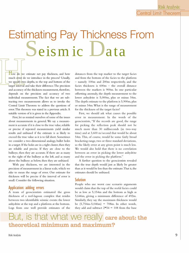
Had we taken the distributions to be triangular(minimum, mode, maximum), the simulation wouldshow that Thickness has a 99% probability range of[1,706.12ft; 2,231.08ft] or [520m; 680m]. In thiscase, we would use:

Top = Triangular (5,046m; 5,100m; 5,154m) andBottom = Triangular (5,646m; 5,700m; 5,754m) andThickness = Bottom – Top The result is approximated by Normal(600m;

31.5m).The P5, P95 interval is [549m; 65m].Theseand other approximations are summarized in Table 1.

Finally, we run this model using the uniform(minimum, maximum) distribution, specificallyuniform (4946m,5054m) for the top and uniform(5,846m, 5,954m) for the bottom. Thanks to theCentral Limit Theorem, the difference can still bereasonably approximated by a normal (not uniform)distribution – although as one can show, thetriangular distribution type actually fits better –namely Normal (600m; 38.5m).The interval rangesshown in the last column of the table were obtainedfrom a simulation with 6,000 iterations.

Summary and refinementsWhen we subtract one random variable fromanother the resulting distribution tends to be

Uncorrelated Normal Triangular Uniform99% confidence [535m,665m] [520m ,680m] [503m, 697m]95% confidence [551m, 649m] [539m, 661m] [515m, 685m]90% confidence [558m, 642m] [549m, 651m] [526m, 674m]

Correlated (r=0.7) Normal Triangular Uniform99% confidence [565m; 635m] [555m, 645m] [533m, 665m]95% confidence [573m, 627m] [566m, 634m] [548m, 652m]90% confidence [578m, 623m] [572m, 629m] [557m,643m]

Table 1. Effect of Distribution Shape on Ranges (maximum, minimum) for Net Pay Thickness

Risk Analysis 11


normal; its coefficient of variation (ratio of standarddeviation to mean) reduces to about 30% from thatof the original variables. When pay thickness isobtained by subtracting two depth measurements,the precision of thickness is better than the precisionof the inputs.Thus rather than compounding errors,the effect is to reduce errors.

One aspect of Monte Carlo simulation thatalways needs to be considered is possible correlationbetween input variables. In the present context, thequestion is whether a large value for Top wouldtypically be paired with a large or small value forBottom.That is, if we overestimate the depth of Top,would we be more likely to overestimate orunderestimate the value of Bottom or would thevalues be uncorrelated (independent)? When theywere asked, the geologists said that if anything, thetwo values would be positively correlated: a largevalue for Top would tend to be paired with a largevalue for Bottom. Essentially, they argued that theywould consistently select the top or the midpoint orthe bottom of a depth curve. How would thatimpact the results?

We reran the simulation using a rank correlationcoefficient of 0.7 between the two inputs in each ofthe three cases (normal, triangular, uniform shapes).The results, shown in the lower portion of Table 1,show a dramatic effect: the error intervals decreaseby nearly 50% from the uncorrelated cases.

Conclusions The Central Limit Theorem (see below) can beapplied to measurement errors from seismicinterpretations.

When specifying a range of error for an estimate,we should be interested in a practical range, one thatwould guarantee the true value would lie in thegiven range 90%, 95% or 99% of the time.

When we estimate thickness by subtracting onedepth from another, the error range of the result isabout 30% smaller than the error range of the depths.

If the depth measurements are positivelycorrelated, as is sometimes thought to be the case,this range of the thickness decreases by another 50%.

The Central Limit TheoremLet Y = X1 + X2 +…+ Xn and Z = Y/n where X1, X2, …, Xnare independent, identical random variables eachwith mean � and standard deviation �.Then:

• both Y and Z are approximately normallydistributed;

• the respective means of Y and Z are n*� and�; and

• the respective standard deviations areapproximately n � and �� n

This approximation improves as n increases.Note that this says the coefficient of variation, theratio of standard deviation to mean, shrinks by afactor of n for Y.

Even if the Xs are not identical orindependent, the result is still approximatelytrue: adding distributions results in a distributionthat is approximately normal even if thesummands are not symmetr ic. Moreover,coefficient of variation diminishes.

When is the approximation not good? Twoconditions will retard this process: a few dominantdistributions, strong correlation among the inputs.Some illustrations may help.

For instance, we take 10 identical lognormaldistributions each having mean 100 and standarddeviation 40 (thus with coefficient of variation,CV, of 0.40).

The sum of these distributions has mean 1,000and standard deviation 131.4 so CV=.131, which isvery close to 0.40/sqrt(10) or 0.127.

On the other hand, if we replace three of thesummands with more dominant distributions, sayeach having a mean of 1,000 and varying standarddeviations of 250, 300 and 400, say, then the sumhas a mean of 3,700 and standard deviation, 575,yielding a CV of .16. The sum of standarddeviations divided by the square root of 10 wouldbe 389, not very close to the actual standarddeviation. It would make more sense to divide thesum by the square of root of 3 acknowledging thedominance of three of the summands. As one canfind by simulation, however, even in this case, thesum is still reasonably symmetric. ◆

We may be more interested in a practical rangethat will cover a large percentage, say 90%, 95% or 99%of the cases.

12 Risk Analysis

Risk Analysis:Bayes’ Theorem

DDDo you know how to revise the probability ofsuccess for a follow up well?

Consider two prospects,A and B, each havinga chance of success, P(A) and P(B). Sometimesthe prospects are independent in the sense thatthe success of one has no bearing on the successof the other.This would surely be the case if theprospects were in different basins. Other times,however, say when they share a common sourcerock, the success of A would cause us to revisethe chance of success of B. Classic probabilitytheory provides us with the notation for the(conditional) probability of B given A, P(B|A), aswell as the (joint) probability of both beingsuccessful, P(A&B).

Our interest lies in the manner in which werevise our estimates. In particular, we will ask:

• how much better can we make the chance ofB when A is successful?

That is, how large can P(B|A) be relative toP(B); and

• if we revise the chance of B upward whenA is a success, how much can or should werevise the chance of B downward when A isa failure?

As we shall see, there are limits to these revisions,stemming from Bayes’Theorem.

Bayes’ Theorem regulates the way two ormore events depend on one another, usingconditional probability, P(A|B), and jointprobability, P(A&B). It addresses independenceand partial dependence between pairs of events.The formal statement, shown here, has numerousapplications in the oil and gas industry.

Bayes’ Theorem1. P(B|A)= P(A|B)*P(B)/P(A)2. P(A) = P(A&B1) + P(A&B2) + … + P(A&Bn), where

B1, B2, …Bn are mutually exclusive andexhaustive

We can rewrite part 2 if we use the fact that:P(A&B) = P(A|B)*P(B)2’. P(A) = P(A|B1)*P(B1) + P(A|B2)*P(B2) +

…+P(A|Bn)*P(Bn)Part 1 says that we can calculate the conditional

probability in one direction, provided we know theconditional probability in the other direction alongwith the two unconditional probabilities. It can bederived from the definition of joint probability,which can be written backward and forward.

P(B|A)P(A) = P(A&B) = P(B&A) = P(A|B)P(B)Part 2 says that if A can happen in conjunction

with one and only one of the Bi’s, then we cancalculate the probability of A by summing thevarious joint probabilities.

There are numerous applications of Bayes’Theorem. Aside from the two drilling prospectsmentioned above, one well-known situation is therole Bayes’Theorem plays in estimating the valueof information, usually done with decision trees.In that context, the revised probabilitiesacknowledge the additional information, whichmight fall into the mutually exclusive andexhaustive categories of good news and bad news(and sometimes no news).

Further, we can define P(~A) to be theprobability that prospect A fails (or in a more generalcontext that event A does not occur). A ratherobvious fact is that

Bayes’ Theorem –

Pitfalls

Bayes’ Theorem regulates the way two or moreevents depend on one another, using conditionalprobability, P(A|B), and joint probability, P(A&B).

Risk Analysis 13

Risk Analysis:Bayes’ Theorem

P(A) + P(~A) = 1, which says thateither A happens or it doesn’t.

The events A and ~A areexhau s t ive and mu tu a l l yexclusive.

Almost as obvious is thesimilar situation

P(A|B) + P(~A|B) = 1, whichsays that once B happens,either A happens or it doesn’t.

Armed with these simpletools, we can point out somecommon pitfalls in estimatingprobabilities for geologicallyrelated prospects.

Pitfall 1: Upgrading the prospect too muchSuppose we believe the prospectsare highly dependent on eachother, because they have acommon source and a common potential seal.

Suppose P(A)=.2, P(B) = .1, and P(B|A)= .6This is the type of revised estimate people tend

to make when they believe A and B are highlycorrelated.The success of A “proves” the commonuncertainties and makes B much more likely.

But, consider the direct application of Bayes’Theorem:

P(A|B) = P(B|A)*P(A)/P(B) = (.6)*(.2)/.1 = 1.2Since no event, conditional or otherwise, can

have a probability exceeding 1.0, we havereached a contradiction, which we can blame onthe assumptions.

What is the problem?When two prospects are highly correlated, theymust have similar probabilities; one cannot betwice as probable as the other. Another way oflooking at this is to resolve the equations:

P(A|B)/P(A) = P(B|A)/P(B), which says that the relativeincrease in probability is identical for both A and B.

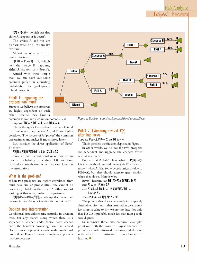
Decision tree interpretationConditional probabilities arise naturally in decisiontrees. For any branch along which there is asequence of chance node, choice node, chancenode, the branches emanating from the secondchance node represent events with conditionalprobabilities. Figure 1 shows a simple example of atwo-prospect tree.

Pitfall 2: Estimating revised P(S) after bad newsSuppose P(A)=.3, P(B) = .2, and P(B|A)= .6

This is precisely the situation depicted in Figure 1.In other words, we believe the two prospects

are dependent and upgrade the chances for Bonce A is a success.

But what if A fails? Then, what is P(B|~A)?Clearly, one should instead downgrade B’s chance ofsuccess when A fails. Some people assign a value toP(B|~A), but they should exercise great cautionwhen they do so. Here is why.

Bayes’Theorem says P(B|-A)=P(-A|B)*P(B)/ P(-A)But P(~A) = 1-P(A) = 0.7and P(~A|B)=1-P(A|B) = 1-P(B|A)*P(A)/ P(B) =

1-.6*.3/.2 = .1Thus P(B|~A) = (.1)*(.2)/.7 = .03The point is that this value already is completely

determined from our other assumptions; we cannotjust assign a value to it – we are too late. Not onlythat, but .03 is probably much less than most peoplewould guess.

In summary, these two common examplespoint out both the power of Bayes’Theorem toprovide us with informed decisions, and the easewith which casual estimates of our chances canlead us. ◆

Figure 1. Decision tree showing conditional probabilities

Divest

Drill A

Fail A

Success A 30%

70%

divest

Drill BSuccess B 3%

Fail B 97%

0

01

00

divest

Drill BSuccess B 60%

Fail B 40%

0

00

00

14 Risk Analysis

Risk Analysis:Invoking Tools

DDDecision trees and Monte Carlo simulation are thetwo principal tools of risk analysis. Sometimes usersapply one tool when the other would be more help-ful. Sometimes it makes sense to invoke both tools.After a brief review of their objectives, methods andoutputs, we illustrate both proper and improperapplications of these well-tested procedures.

Decision trees:Objectives, methodology, resultsDecision trees select between competing alternativechoices, finding the choice – and subsequent choicesalong a path – which either maximizes value orminimizes cost.

The output of a tree is a combination of theoptimal path and the expected value of that path.Thus, decision trees yield one number.The rules ofsolving the tree force acceptance of the path with thehighest expected value, regardless of its uncertainty.

In theory, preference functions can be used inplace of monetary values, but in practice, usersseldom go to this level.

Decision trees allow limited sensitivity analysis,in which the user perturbs either some of theassigned values or some of the assignedprobabilities, while monitoring the overall treevalue. Typically, the user varies one or twoparameters simultaneously and illustrates the resultswith graphs in the plane (how the tree valuechanges when one assigned value is varied) or inspace (how the tree value varies when two assigned

values are varied together).The traditional tornadochart also is used to show how each perturbedvariable affects the tree value when all other valuesare held fixed. This chart takes its name from theshape it assumes when the influences of theperturbed variables are stacked as lines or bars, withthe largest on top.

Trees, along with their cousins influence diagrams,are particularly popular for framing problems andreaching consensus. For small to moderate sizeproblems, the picture of the tree is an effective meansof communication.

One of the most important problem typessolvable by trees is assessing the value of informa-tion. In this case, one possible choice is to buyadditional information (seismic interpretation, welltest, logs, pilot floods). Solving the tree with andwithout this added-information branch and takingthe difference between the two expected valuesyields the value added by the information. If theinformation can be bought for less than its imputedvalue, it is a good deal.

Monte Carlo simulation:Objectives, methodology, resultsMonte Carlo models focus on one or moreobjective functions or outputs. Favorite outputsinclude reserves, total cost, total time and netpresent value (NPV). Their respective inputsinclude areal extent, net pay and porosity; lineitem costs; activity times; and production

Decision Trees vs.

Monte CarloSimulation

Trees, along with their cousins influence diagrams,are particularly popular for framing problems andreaching consensus.

Risk Analysis 15


forecasts, price forecasts, capital forecasts andoperating expense forecasts.

A Monte Carlo (MC) simulation is the processof creating a few thousand realizations of the modelby simultaneously sampling values from the inputdistributions.The results of such an MC simulationtypically include three items: a distribution for eachdesignated output, a sensitivity chart listing the keyvariables ranked by their correlation with a targetedoutput, and various graphs and statistical summariesfeaturing the outputs.

Unlike decision trees, MC simulations do notexplicitly recommend a course of action or make adecision. Sometimes, however, when there arecompeting alternatives, an overlay chart is used todisplay the corresponding cumulative distributions,in order to compare their levels of uncertainty andtheir various percentiles.

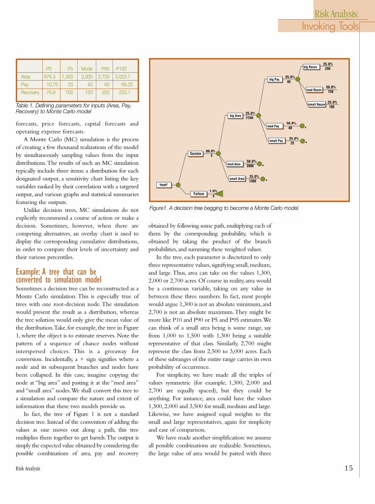
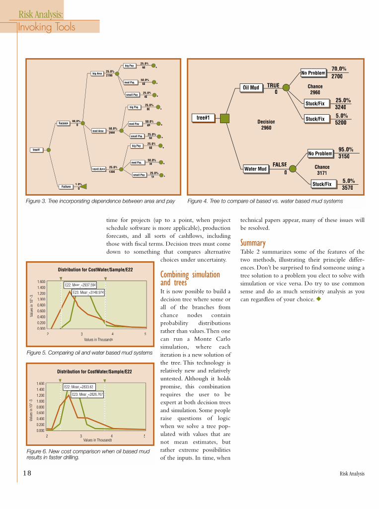
Example: A tree that can be converted to simulation modelSometimes a decision tree can be reconstructed as aMonte Carlo simulation. This is especially true oftrees with one root-decision node. The simulationwould present the result as a distribution, whereasthe tree solution would only give the mean value ofthe distribution.Take, for example, the tree in Figure1, where the object is to estimate reserves. Note thepattern of a sequence of chance nodes withoutinterspersed choices. This is a giveaway forconversion. Incidentally, a + sign signifies where anode and its subsequent branches and nodes havebeen collapsed. In this case, imagine copying thenode at “big area” and pasting it at the “med area”and “small area” nodes.We shall convert this tree toa simulation and compare the nature and extent ofinformation that these two models provide us.

In fact, the tree of Figure 1 is not a standarddecision tree. Instead of the convention of adding thevalues as one moves out along a path, this treemultiplies them together to get barrels.The output issimply the expected value obtained by considering thepossible combinations of area, pay and recovery

obtained by following some path, multiplying each ofthem by the corresponding probability, which isobtained by taking the product of the branchprobabilities, and summing these weighted values.

In the tree, each parameter is discretized to onlythree representative values, signifying small,medium,and large.Thus, area can take on the values 1,300,2,000 or 2,700 acres.Of course in reality, area wouldbe a continuous variable, taking on any value inbetween these three numbers. In fact, most peoplewould argue 1,300 is not an absolute minimum, and2,700 is not an absolute maximum.They might bemore like P10 and P90 or P5 and P95 estimates.Wecan think of a small area being is some range, sayfrom 1,000 to 1,500 with 1,300 being a suitablerepresentative of that class. Similarly, 2,700 mightrepresent the class from 2,500 to 3,000 acres. Eachof these subranges of the entire range carries its ownprobability of occurrence.

For simplicity, we have made all the triples ofvalues symmetric (for example, 1,300, 2,000 and2,700 are equally spaced), but they could beanything. For instance, area could have the values1,300, 2,000 and 3,500 for small, medium and large.Likewise, we have assigned equal weights to thesmall and large representatives, again for simplicityand ease of comparison.

We have made another simplification:we assumeall possible combinations are realizable. Sometimes,the large value of area would be paired with three

P0 P5 Mode P95 P100

Area 976.3 1,300 2,000 2,700 3,023.7

Pay 10.75 20 40 60 69.25

Recovery 76.9 100 150 200 223.1

Table 1. Defining parameters for inputs (Area, Pay,Recovery) to Monte Carlo model

Failure

Success

small Area

1.0%%0

tree#1

99.0%0

med Area

25.0%1300

50.0%2000 +

+

big Area

small Pay

25.0%2700

med Pay

25.0% 20

50.0% 40 +

+

big Pay

small Recov

25.0% 60

med Recov

25.0% 100

50.0% 150

big Recov25.0% 200

Figure1. A decision tree begging to become a Monte Carlo model.

16 Risk Analysis


relatively large values of pay, in thebelief these two parameters aredependent.This is simple to accom-modate in a tree.

Building the corresponding Monte Carlo simulation modelConverting to an appropriateMonte Carlo model requiresfinding a suitable distribution foreach of the three inputs – area, payand recovery. In light of thediscussion above, we took thesmall values to be P5 and the bigvalues to be P95.We also selected

triangular distributions is each case (which is howwe obtained our P0 and P100 values). Theresulting distributions are shown in Table 1.

From the tree analysis,we can calculate the expectedvalue as well as finding the two extreme values (smallestand largest) and their respective probabilities:

Expected value 12MMSTBMinimum value 2.6MMSTB, P(min) = 1/64Maximum value 32.4 MMSTB, P(max) = 1/64What we cannot determine from the tree analysis is

how likely the reserves would exceed 5 MMSTB, howlikely they would be between 5 MMSTB and 15MMSTB, how likely they would be less than 12MMSTB, and so on.

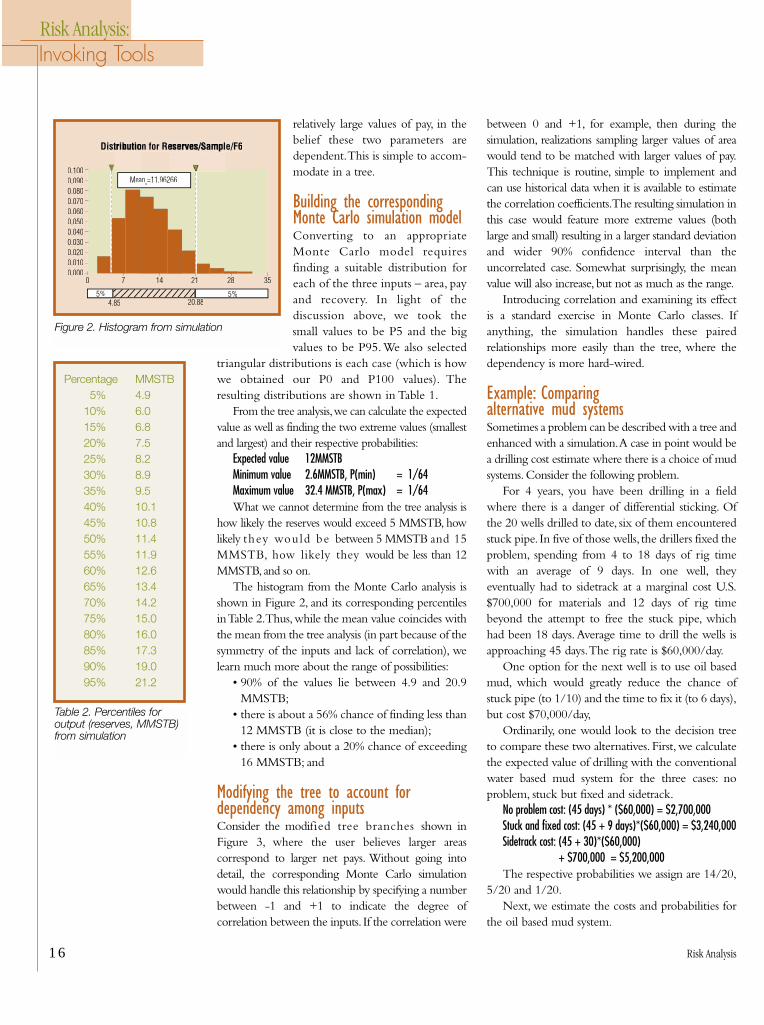
The histogram from the Monte Carlo analysis isshown in Figure 2, and its corresponding percentilesin Table 2.Thus,while the mean value coincides withthe mean from the tree analysis (in part because of thesymmetry of the inputs and lack of correlation), welearn much more about the range of possibilities:

• 90% of the values lie between 4.9 and 20.9MMSTB;

• there is about a 56% chance of finding less than12 MMSTB (it is close to the median);

• there is only about a 20% chance of exceeding16 MMSTB; and

Modifying the tree to account fordependency among inputsConsider the modified tree branches shown inFigure 3, where the user believes larger areascorrespond to larger net pays. Without going intodetail, the corresponding Monte Carlo simulationwould handle this relationship by specifying a numberbetween -1 and +1 to indicate the degree ofcorrelation between the inputs. If the correlation were

between 0 and +1, for example, then during thesimulation, realizations sampling larger values of areawould tend to be matched with larger values of pay.This technique is routine, simple to implement andcan use historical data when it is available to estimatethe correlation coefficients.The resulting simulation inthis case would feature more extreme values (bothlarge and small) resulting in a larger standard deviationand wider 90% confidence interval than theuncorrelated case. Somewhat surprisingly, the meanvalue will also increase, but not as much as the range.

Introducing correlation and examining its effectis a standard exercise in Monte Carlo classes. Ifanything, the simulation handles these pairedrelationships more easily than the tree, where thedependency is more hard-wired.

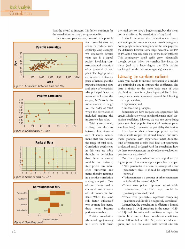
Example: Comparing alternative mud systemsSometimes a problem can be described with a tree andenhanced with a simulation.A case in point would bea drilling cost estimate where there is a choice of mudsystems. Consider the following problem.

For 4 years, you have been drilling in a fieldwhere there is a danger of differential sticking. Ofthe 20 wells drilled to date, six of them encounteredstuck pipe. In five of those wells, the drillers fixed theproblem, spending from 4 to 18 days of rig timewith an average of 9 days. In one well, theyeventually had to sidetrack at a marginal cost U.S.$700,000 for materials and 12 days of rig timebeyond the attempt to free the stuck pipe, whichhad been 18 days.Average time to drill the wells isapproaching 45 days.The rig rate is $60,000/day.

One option for the next well is to use oil basedmud, which would greatly reduce the chance ofstuck pipe (to 1/10) and the time to fix it (to 6 days),but cost $70,000/day,

Ordinarily, one would look to the decision treeto compare these two alternatives. First, we calculatethe expected value of drilling with the conventionalwater based mud system for the three cases: noproblem, stuck but fixed and sidetrack.

No problem cost: (45 days) * ($60,000) = $2,700,000Stuck and fixed cost: (45 + 9 days)*($60,000) = $3,240,000Sidetrack cost: (45 + 30)*($60,000)

+ $700,000 = $5,200,000The respective probabilities we assign are 14/20,

5/20 and 1/20.Next, we estimate the costs and probabilities for

the oil based mud system.

Percentage MMSTB5% 4.9

10% 6.015% 6.820% 7.525% 8.230% 8.935% 9.540% 10.145% 10.850% 11.455% 11.960% 12.665% 13.470% 14.275% 15.080% 16.085% 17.390% 19.095% 21.2

Table 2. Percentiles for output (reserves, MMSTB)from simulation

Distribution for Reserves/Sample/F6Distribution for Reserves/Sample/F6

0.1000.0900.0800.0700.0600.0500.0400.0300.0200.0100.000

0 7 14 21 28 35

5% 5%4.85 20.88

Meanv=11.96266

Figure 2. Histogram from simulation

Risk Analysis 17

No problem cost: (45 days)*($70,000) = $ 3,150,000Cost when stuck pipe: (45+6)*($70,000) = $3,570,000The respective probabilities are 9/10 and 1/10.The resulting tree is shown in Figure 3, indicat-

ing the correct decision would be to use the waterbased mud with an expected value of $2,960,000rather than the oil-based alternative with anexpected value of $ 3,171,000.

The Monte Carlo approach The Monte Carlo model shown in Table 3 capturesthe same information as the tree model, but uses itdifferently. Specifically, the simulation model allowsthe user to estimate ranges for the various activitiesand costs. For comparison purposes, the historicalminimum and maximum values are treated as P5 andP95 to build input distributions, with the option forthe user to set these percentages. Most peopleestimating ranges of this sort, especially costestimators, tend toward right-skewed distributions.

Certainly, in this model, we should care aboutmore than just the expected value. For instance,we may want to know the probability of exceed-ing a certain value, such as $4,000,000.We may alsowant to question other inputs (see discussionbelow).

Figure 5 shows the comparison with the assump-tions taken from the problem statement. Figure 6shows a variation where the oil-based mud takes only40 days on average to drill and the chance of sidetrackwith water mud is 10%, not 5%. The differencebetween the two cases is clear: as the probability ofsidetracking increases, the oil-based mud presents aless risky alternative (the density function ofoutcomes is much narrower). Similar analyses can bemade easily in the Monte Carlo model.

Which model is better in this instance?Both the tree and the simulation offer informationto the user and to the larger audience of thepresentations that can be prepared from them.Thetree emphasizes the two contrasting choices andidentifies the extreme outcomes and their prob-abilities of occurrence. It is both simple and effec-tive.Yet, the tree does not explicitly acknowledge theunderlying uncertainty in each of the contributoryestimates (such as days for problem free drilling, costof mud system,days for trying to free the stuck pipe,days for sidetracking). The user can handle theseuncertainties – one or two at a time – by using thetree framework to do a trial-and-error sensitivity

analysis, and any userwould be remiss inavoiding this.But theoverall uncertainty ismade more explicitin the Monte Carlosimulation, wherethe very nature ofthe model begs theuser to specify therange of uncertainty.

On balance, if I had to pick one model, I wouldpick the simulation, in part because I have had farbetter results analyzing uncertainty and presentingthe details to management when I use simulation.Butwhatever your preference in tools, for this problemthe combination of both a tree and the simulationseems to be the most useful.

Which model is better in general?When is Monte Carlo more appropriate? Ingeneral, Monte Carlo seems to have more variedapplications. Any (deterministic) model you canbuild in a spreadsheet can be converted to aMonte Carlo model by replacing some of theinput values with probability distributions. Thus,in addition to the popular resource and reservevolumetric product models, people build MonteCarlo models for costs of drilling and facilities,

P(StuckWater) 30.0%P(SideTrack) 5% LowP 5P(StuckOil) 5% HighP 95

Sample Plow Mode PhighDayRateWater $ 60 60 60 60DayRateOil $ 70 70 70 70DaysWater_NoStuck 45.0 40.5 45 49.5DaysOil_NoStuck 45.0 40.5 45 49.5DaysSideTrack 12.0 10.8 12 13.2StuckWater? 0 1 = stuckSideTrack? 0 1=sidetrackStuckOil? 0 1 = stuckDayWater_Stuck 10.4 4 8 18DaysOil_Stuck 7.2 3 6 12ExtraCost_ST 700.0CostWater $ 2,700 CostOil $ 3,150 TimeWater 45.0TimeOil 45.0

Table 3. Monte Carlo model to compare oil based and water based mud systems


Decision Trees Monte Carlo simulationObjectives make decisions quantify uncertaintyInputs discrete scenario distributionsSolution driven by EV run many casesOutputs choice and EV distributionsDependence limited treatment rank correlation

Table 4. Comparison between Decision trees and Monte Carlosimulation

18 Risk Analysis


time for projects (up to a point, when projectschedule software is more applicable), productionforecasts, and all sorts of cashflows, includingthose with fiscal terms. Decision trees must comedown to something that compares alternative

choices under uncertainty.

Combining simulationand treesIt is now possible to build adecision tree where some orall of the branches fromchance nodes containprobability distributionsrather than values.Then onecan run a Monte Carlosimulation, where eachiteration is a new solution ofthe tree. This technology isrelatively new and relativelyuntested. Although it holdspromise, this combinationrequires the user to beexpert at both decision treesand simulation. Some peopleraise questions of logicwhen we solve a tree pop-ulated with values that arenot mean estimates, butrather extreme possibilitiesof the inputs. In time, when

technical papers appear, many of these issues willbe resolved.

SummaryTable 2 summarizes some of the features of thetwo methods, illustrating their principle differ-ences. Don’t be surprised to find someone using atree solution to a problem you elect to solve withsimulation or vice versa. Do try to use commonsense and do as much sensitivity analysis as youcan regardless of your choice. ◆

E22: Meanv=2937.594

E23: Meanv=3148.974

Distribution for CostWater/Sample/E22

1.6001.4001.2001.0000.8000.6000.4000.2000.000

2 3 4 5

Valu

es in

10

-3vv

Values in Thousands

Figure 5. Comparing oil and water based mud systems

Distribution for CostWater/Sample/E22

1.6001.4001.2001.0000.8000.6000.4000.2000.000

2 3 4 5

E22: Meanv=2833.63

E23: Meanv=2826.767

Values in Thousands

Valu

es in

10

-3vv

Figure 6. New cost comparison when oil based mudresults in faster drilling.

Failure

Success

small Area

1.0%%0

tree#1

99.0%0

med Area

25.0%1300

50.0%2000

25.0%2700

small Pay

med Pay

25.0% 40

50.0% 60 +

+

big Pay25.0% 90 +

small Pay

med Pay

25.0% 30

50.0% 40 +

+

big Pay25.0% 80 +

big Area

small Pay

med Pay

25.0% 15

50.0% 30 +

+

big Pay25.0% 60 +

Figure 3. Tree incorporating dependence between area and pay

Water Mud

Oil Mud

FALSE0

tree#1

TRUE0

Stuck/Fix

No Problem

5.0%3570

95.0%3150

Chance3171

Decision2960

Stuck/Fix

No Problem

25.0%3240

70.0%2700

Chance2960

Stuck/Fix 5.0%5200

Figure 4. Tree to compare oil based vs. water based mud systems

19 Risk Analysis

Risk Analysis:Correlation

WWWhat is correlation?Often, the input variables to our Monte Carlo

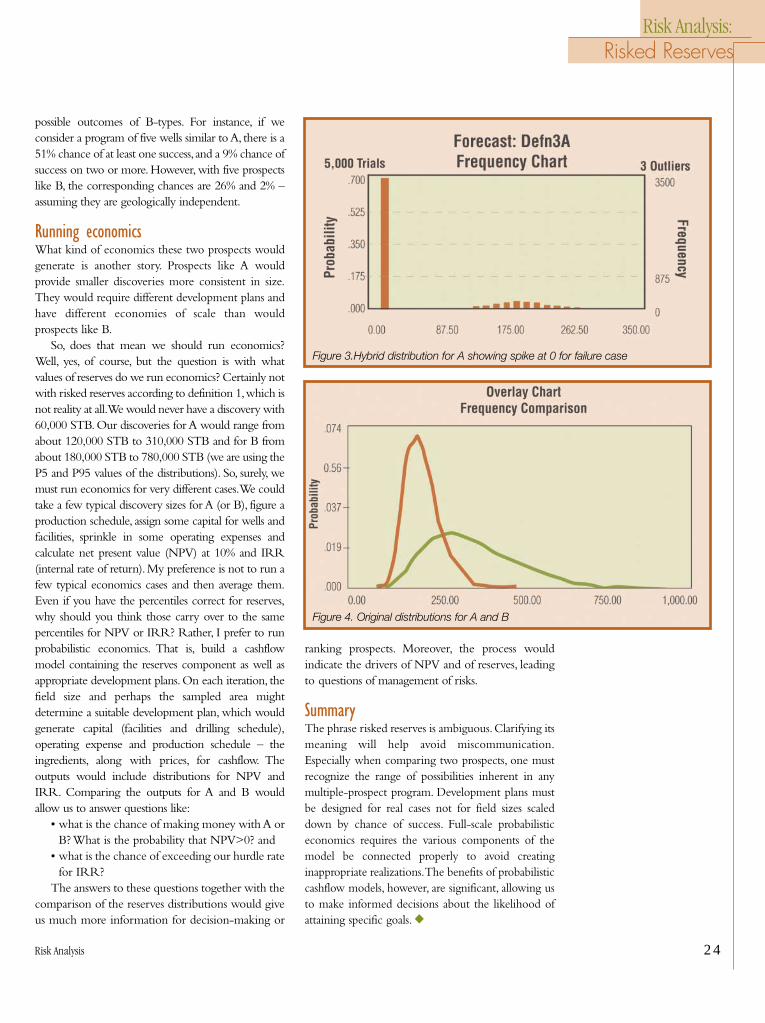
models are not independent of one another. Forexample, consider a model that estimates reserves bytaking the product of area (A), average net pay (h) andrecovery (R).In some environments, the structures withlarger area would tend to have thicker pay.This propertyshould be acknowledged when samples are selectedfrom the distributions for A and h.Moreover, a databaseof analogues would reveal a pattern among the pairs ofvalues A and h. Think of a cross-plot with a generaltrend of increasing h when A increases, as shown inFigure 1. Such a relationship between two variables canbest be described by a correlation coefficient.

Examples of correlated variablesTypical pairs of correlated parameters are:

• daily high temperature and air conditioningcost for a personal residence in New Orleans;

• measured depth to total depth and drilling costfor wells in the North Sea;

• porosity and water saturation assigned tocompletion intervals for wells in a given reservoir;

• porosity and permeability assigned to completionintervals for wells in a given reservoir;

• operating cost and production rate;• the permeability-thickness product and the

recovery efficiency for gas wells in a given field;• height and weight of 10-year old males in the

United States;• propane price and ethane price on Friday

afternoon NYMEX;• propane price and Brent crude price; and• square footage and sales price of used houses

sold in Houston in 1995.

Definition of correlation coefficientTwo variables are said to have correlation coefficientr if:

where:

and

Excel has a function, sumproduct ({x},{y}), thattakes the sum of the products of the correspondingterms of two sequences {x} and {y}. Thus,covariance is a sumproduct.

The value of r lies between –1 (perfect negativecorrelation) and +1 (perfect positive correlation).Although there are tests for significance of thecorrelation coefficient, one of which we mentionbelow, statistical significance is not the point of thisdiscussion. Instead, we focus on the practical side,asking what difference it makes to the bottom lineof a Monte Carlo model (e.g., estimating reserves orestimating cost of drilling a well) whether weinclude correlation. As we shall see, a correlationcoefficient of 0.5 can make enough of a differencein some models to worry about it.

Before we illustrate the concept, we need topoint out that there is an alternate definition.

Two types of correlation - ordinary and rankWhen correlation was formally defined in the late 19thcentury, statisticians recognized one or a few pointswith extreme values could unduly influence theformula for calculating r. Specifically, the contributionof a pair (xi,yi) to the covariance, namely

could be an order of magnitude larger than theother terms.

Charles Spearman introduced an alternative for-mulation, which he labeled “distribution-free” andcalled it the rank-order correlation coefficient, incontrast to the Pearson coefficient defined above.To

When Does Correlation

Matter?

r� cov(x, y)

�x * �y

Cov�(1/n) � (xi �x)*(yi �y)

varx�(1/n) � (xi �x)2

�x� varx

(xi �x) * (yi �y)

Risk Analysis 20


obtain the Spearman coefficient, one replaces theoriginal data with their ranks then calculates thecorrelation coefficient using the ranks.Tables 1 and 2provide a simple example illustrating both methods.

Impact of correlation on the output of a modelWhat does correlation do to the bottom line? Doesit alter the distribution of reserves or cost or netpresent value (NPV), which is, after all, the objec-tive of the model? If so, how?

We can make some generalizations, but rememberOliver Wendell Holmes’s admonition, “No generali-zation is worth a damn…including this one.”

First, a positive correlation between two inputswill result in more pairs of two large values andmore pairs of two small values. If those variables aremultiplied together in the model, for example, areserves model, then this results in more extremevalues of the output.

Even in a summation or aggregation model(aggregating production from different wells orfields, aggregating reserves, estimating total cost bysumming line items and estimating total time),positive correlation between two summands willcause the output to be more disperse.

In short, in either a product or aggregation model,a positive correlation between two pairs of variableswill increase the standard variation of the output.

The surprising thing is what happens to themean value of the output when correlation isincluded in the model.

For product models, positive correlation betweenfactors will increase the mean value of the output.Foraggregation models, the mean value of the output isnot affected by correlation among the summands.

Let us hasten to add that many models are neitherpure products nor pure sums, but rather complexalgebraic combinations of the various inputs.

Example 1. Correlating parameters in avolumetric reserves modelA simple example will illustrate the properties of aproduct model.

A common classroom exercise to illustrate theeffect of correlation on reserves uses the model:

N = AhRWith:A = Triangular (1000,2000,4000)h = Triangular (20,50,100)R = Triangular (80,120,200)

Each student is assigned a correlation coefficient,from 0 to 0.7, and uses it to correlate A with h and hwith r (the same coefficient for both pairs).The studentsrun the simulations using both these correlations andcall out their results, which are tallied in Table Y:

Now of course, even if both correlations werewarranted, it would be unlikely they would beidentical. Nevertheless, we must note the standarddeviation can increase by as much as 50% and themean by about 10% under substantial correlation.

The message is clear: pay attention to correlationsin volumetric product models if you care about thedanger of easily underestimating the mean value by5% or more, or if you care about understating theinherent uncertainty in the prospect by 30% or 40%.

Almost as important: often correlation makes littledifference in the results.We just need to check it out.

While it may not be obvious, nearly all thecorrelations in reserves models cause the dispersion

Table 1. Area, porosity, and gas saturation (and their ranks) for 13 reefal structuresName Area, km^2 Porosity Sg Rank_Area Rank_por Rank_Sg

S1 10 0.12 0.77 3 1 3M1 24 0.12 0.85 6 1 10A1 37 0.13 0.87 9 3 11P2 6 0.14 0.81 1 4 6K3 28.8 0.14 0.91 7 5 13D 6 0.15 0.61 1 6 1U1 34 0.15 0.82 8 7 8P1 13 0.16 0.81 5 8 6K2 60 0.16 0.78 12 9 4K4 11 0.17 0.83 4 10 9K1 58 0.18 0.80 11 11 5U2 48 0.22 0.75 10 12 2Z1 108 0.22 0.89 13 12 12

Table 2. Correlation and Rank Correlation coefficients for the reefal structure data.Ordinary r Area Porosity Sg Rank r Area Porosity SgArea 1 Area 1Porosity 0.67 1 Porosity 0.57 1Sg 0.36 -0.02 1 Sg 0.28 -0.12 1

r mean StDev0 17.5 7.7.1 17.9 8.6.2 18.1 9.1.3 18.3 9.7.4 18.6 10.5.5 18.8 10.9.6 19.0 11.3.7 19.3 11.9

21 Risk Analysis

(and the mean) to increase. It is far less common forthe correlations to have the opposite effect.

In more complex models, however, it is possiblefor correlations toactually reduce un-certainty. One examplewe discovered severalyears ago is a capitalproject involving con-struction and operationof a gas-fired electricplant. The high positivecorrelation betweenprice of natural gas (theprincipal operating cost)and price of electricity(the principal factor inrevenue) will cause theoutput, NPV, to be farmore modest in range(on the order of 50%)when the correlation isincluded, making theinvestment less risky.

With a cost model,adding correlationsbetween line items isone of several refine-ments that can increasethe range of total costs.Correlation coefficientsin this case are oftenthought to be higherthan those in reservemodels. For instance,steel prices can influ-ence numerous lineitems, thereby resultingin a positive correlationamong the pairs. Oneof our clients used acost model with a matrixof risk factors vs. lineitems. When the samerisk factor influencedtwo or more line items,these items becamepositively correlated.

Positive correlation(the usual type) amongline items will cause

the total cost to have a bigger range, but the meancost is unaffected by correlation of any kind.

It should be noted that correlation can have aserious impact on cost models in terms of contingency.Some people define contingency for the total project asthe difference between some large percentile, say P85or P90,and a base value like P50 or the mean total cost.This contingency could easily grow substantially,though, because when we correlate line items, themean (and to a large degree the P50) remainsunchanged but the dispersion (typically) increases.

Estimating the correlation coefficientOnce you decide to include correlation in a model,you must find a way to estimate the coefficients.Thisissue is similar to the more basic issue of whatdistribution to use for a given input variable. In bothcases, you can resort to one or more of the following:

• empirical data;• experience; and• fundamental principles.Sometimes we have adequate and appropriate field

data,in which case,we can calculate the (rank order) cor-relation coefficient. Likewise, we can use curve-fittingprocedures (both popular Monte Carlo software pack-ages have them) to generate the probability distribution.

If we have no data or have appropriate data butonly a small sample, we should temper our auto-matic processes with experience. What does thiskind of parameter usually look like: is it symmetricor skewed, small or large? And for correlation, howdo these two parameters usually relate to each other:positively or negatively?

Once in a great while, we can appeal to thathigher power: fundamental principles. For example:

• “this parameter is a sum or average of otherparameters; thus it should be approximatelynormal;”

• “this parameter is a product of other parameters– it should be skewed right;”

• “these two prices represent substitutablecommodities, therefore they should bepositively correlated;” and

• “these two parameters represent competingquantities and should be negatively correlated.”

Remember, the correlation coefficient is limitedto the range [-1,+1].Anything in the range [-0.15,+0.15] could be noise and is unlikely to impact theresults. It is rare to have correlation coefficientsabove 0.8 or below –0.8. So, make an educatedguess, and run the model with several alternate


Positive correlationPositive correlation

Area0 500 1,000 1,500 2,00 2,500 3,000

Pay

120100806040200

Figure 1. Correlation between Area and Pay

Positive correlationPositive correlation

0 20 40 60 80 100 120

0.240.220.200.180.160.140.120.10

Figure 2. Original data, r = 0.67

RR

1 2 3 4 5 6 7 8 9 10 11 12 13

13121110

98

6

4

2

Figure 3. Ranks of data r = 0.57

Correlations for NPVCorrelations for NPV

Production1/D4

Investment/D3

Price1/D6

Decline Rate/D5

-1 -0.5 0 0.5 1

Correlation Coefficients

0.694

-0.528

0.432

-0.074

Figure 4. Sensitivity chart

Risk Analysis 22

values and document the results. You may notresolve the issue, but you can defuse it.

Another use of correlation: SensitivityOne argument for studying correlation is to betterunderstand sensitivity analysis. Figure 4 shows onecommon type of sensitivity chart, sometimes called atornado chart. In this case, the numbers represent rankcorrelation coefficients between the target outputvariable (in case a model has two or more outputs) andeach of the inputs. A negative correlation coefficientindicates a model input that tends to increase as theoutput decreases and vice versa. Thus, as capital getslarge, NPV tends to get small. The relationship isproperly described by correlation, because the otherthree inputs also affect NPV. Simply knowing thatcapital is large does not force NPV to have a certainsmall value. But given a particular, large value of capitalmight limit the range of NPV to a smallish part of theentire NPV range, a fact made clear by Figure 5.

SummaryThings to remember:

• correlation is easy tocalculate in Excel (thefunction Correl);

• there are two typesof correlation coeffi-cients: ordinary (Pear-son) and rank-order(Spearman). Theytend to differ when one or both the variables ishighly skewed;

• correlation might matter; it depends on the typeof model and the strength of the correlation;

• correlation always will affect the standarddeviation, often but not always increase it;

• correlation will affect the mean value of aproduct; and

• correlation is useful to describe sensitivity ofoutput to inputs. ◆


Figure 5. Negative correlation: investment and NPV

23 Risk Analysis

Risk Analysis:Risked Reserves

RRRisked reserves” is a phrase we hear a lot these days.It can have at least three meanings:

1. risked reserves might be the product of theprobability of success,P(S), and the mean valueof reserves in case of a discovery. In this case,risked reserves is a single value;

2. risked reserves might be the probabilitydistribution obtained by scaling down all thevalues by a factor of P(S); or

3. risked reserves might be a distribution with aspike at 0 having probability P(S) and a reducedprobability distribution of the success case.

Take as an example Exploration Prospect A. Ithas a 30% chance of success. If successful, then itsreserves can be characterized as in Figure 1, alognormal distribution with a mean of 200,000STB (stock tank barrels) and a standard deviationof 40,000 STB. Then:

• definition 1 yields the single number0.3*200,000 = 60,000 STB;

• definition 2 yields a lognormal definition witha mean of 60,000 and a standard deviation of12,000 (See Figure 2); and

• definition 3 is the hybrid distribution shown inFigure 3. By contrast, suppose another prospect,B, has a 15% chance of success and a reservesdistribution with a mean of 400,000 STB and astandard deviation of 200,000 STB.Then underdefinition 1,B would yield the same risk reservesas A, 0.15*400,000 = 60,000 STB. However, considerFigure 2, which shows how B would be scaledcompared with A,with the same mean but largerstandard deviation.And Figure 4 shows how theoriginal distributions compare.

Assigning these two prospects the same numberfor the purpose of any sort of ranking could bemisleading. Prospect B is much riskier, both in thesense that it has only half the probability of successthan does A, and also because even if it is a success, therange of possible outcomes is much broader. In fact,the P10,where P=Percentile,of Prospect B equals theP50 of Prospect A.Thus, if you drilled several ProspectA types,for fully half of your successes (on average),thereserves would be less than the 10th percentile of oneprospect B.

The only thing equal about Prospects A and B isthat, in the long run, several prospects similar toProspect A would yield the same average reserves asseveral other prospects like B. Even this is deceptive,because the range of possible outcomes for severalprospects like A is much different from the range of

Beware of

Risked Reserves

““

Figure 1.Lognormal distribution for Prospect A reserves

Figure 2.Comparing the original distributions for A and B

Risk Analysis 24

Risk Analysis:Risked Reserves

possible outcomes of B-types. For instance, if weconsider a program of five wells similar to A, there is a51% chance of at least one success,and a 9% chance ofsuccess on two or more. However, with five prospectslike B, the corresponding chances are 26% and 2% –assuming they are geologically independent.

Running economicsWhat kind of economics these two prospects wouldgenerate is another story. Prospects like A wouldprovide smaller discoveries more consistent in size.They would require different development plans andhave different economies of scale than wouldprospects like B.

So, does that mean we should run economics?Well, yes, of course, but the question is with whatvalues of reserves do we run economics? Certainly notwith risked reserves according to definition 1,which isnot reality at all.We would never have a discovery with60,000 STB. Our discoveries for A would range fromabout 120,000 STB to 310,000 STB and for B fromabout 180,000 STB to 780,000 STB (we are using theP5 and P95 values of the distributions). So, surely, wemust run economics for very different cases.We couldtake a few typical discovery sizes for A (or B), figure aproduction schedule, assign some capital for wells andfacilities, sprinkle in some operating expenses andcalculate net present value (NPV) at 10% and IRR(internal rate of return).My preference is not to run afew typical economics cases and then average them.Even if you have the percentiles correct for reserves,why should you think those carry over to the samepercentiles for NPV or IRR? Rather, I prefer to runprobabilistic economics. That is, build a cashflowmodel containing the reserves component as well asappropriate development plans.On each iteration, thefield size and perhaps the sampled area mightdetermine a suitable development plan, which wouldgenerate capital (facilities and drilling schedule),operating expense and production schedule – theingredients, along with prices, for cashflow. Theoutputs would include distributions for NPV andIRR. Comparing the outputs for A and B wouldallow us to answer questions like:

• what is the chance of making money with A orB? What is the probability that NPV>0? and

• what is the chance of exceeding our hurdle ratefor IRR?

The answers to these questions together with thecomparison of the reserves distributions would giveus much more information for decision-making or

ranking prospects. Moreover, the process wouldindicate the drivers of NPV and of reserves, leadingto questions of management of risks.

SummaryThe phrase risked reserves is ambiguous.Clarifying itsmeaning will help avoid miscommunication.Especially when comparing two prospects, one mustrecognize the range of possibilities inherent in anymultiple-prospect program. Development plans mustbe designed for real cases not for field sizes scaleddown by chance of success. Full-scale probabilisticeconomics requires the various components of themodel be connected properly to avoid creatinginappropriate realizations.The benefits of probabilisticcashflow models, however, are significant, allowing usto make informed decisions about the likelihood ofattaining specific goals. ◆

Figure 3.Hybrid distribution for A showing spike at 0 for failure case

Figure 4. Original distributions for A and B

Murtha, J. - Risk Analysis for the Oil Industry

Documents

additional

cousins influence

central limit

monte carlo

bayes theorem

monte carlo

monte carlo

larger standard