Munipl~ Track Digital Magnetic Recording System. - CORE

Channel Coding· Techniques for a· Munipl~ Track

Digital Magnetic Recording System.

Paul 1 l"ames Bavey

"• '''"' -. _, ._ < • I :.,,,

·, , __ , t t ' ·, ~ _ '' ' · "-_ ' ' • I • · , :1

A thesis subinittedlto'the Bniversicy. o:EP.Iymol)th t: ' , 1 ' • ' .. ' f I '

, 1 , ~ r ~ • ~ I

in partiatfulfilment for'the degr,ee:of :. ,. ~ · ' ' ~ I ,· o

I . o i;

DO€'F0R._(i)F PHIUlSOPIJY

Sponsoring Establlslimerit:

School of·Electronic, Communication and !Electrical Engineering

Faculty of Technology

.. • ' ' ' ' 1

; • • .,, ' 1 • ' ; l l ' • ! 'l i 1 b •. •' • !.I ',

Collaborating Establishment:

Hewlett Packard, Computer. Peripheralsi)ivision (Bristol)

Octob~r. 1994

14. NOV. 19911 T UNIVERSITY OF PL Y,MOUJTH

LIBRARY SERVICES Item

9co ;~~ltls991 No. ' Class h:_ ... \cL.\. ~~c~ No.

Contl. )(110211 i-.....,l.f-1 lt-No.

I

~ I

REFERENCE ONLY '

Channel Coding Techniques for a Multiple Track Digital Magnetic Recording System

by Paul James Davey

Abstract

In magnetic recording greater area) bit packing densities are achieved through increasing track density by reducing space between and width of the recording tracks, and/or reducing the wavelength of the recorded information. This leads to the requirement of higher precision tape transport mechanisms and dedicated coding circuitry.

A TMS320 10 digital signal processor is applied to a standard low-cost, low precision, multiple-track, compact cassette tape recording system. Advanced signal processing and coding techniques are employed to maximise recording density and to compensate for the mechanical deficiencies of this system. Parallel software encoding/decoding algorithms have been developed for several Run-Length Limited modulation codes. The results for a peak detection system show that Bi-Phase L code can be reliably employed up to a data rate of 5kbits/secondltrack. Development of a second system employing a TMS32025 and sampling detection permitted the utilisation of adaptive equalisation to slim the readback pulse. Application of conventional read equalisation techniques, that oppose inter-symbol interference, resulted in a 30% increase in performance.

Further investigation shows that greater linear recording densities can be achieved by employing Partial Response signalling and Maximum Likelihood Detection. Partial response signalling schemes use controlled inter-symbol interference to increase recording density at the expense of a multi-level read back waveform which results in an increased noise penalty. Maximum Likelihood Sequence detection employs soft decisions on the readback waveform to recover this loss. The associated modulation coding techniques required for optimised operation of such a system are discussed.

Two-dimensional run-length-limited (d, ky) modulation codes provide a further means of increasing storage capacity in multi-track recording systems. For example the code rate of a single track run length-limited code with constraints (1, 3), such as Miller code, can be increased by over 25% when using a 4-track two-dimensional code with the same d constraint and with the k constraint satisfied across a number of parallel channels. The k constraint along an individual track, kx, can be increased without loss of clock synchronisation since the clocking information derived by frequent signal transitions can be sub-divided across a number of, y, parallel tracks in terms of a Icy constraint. This permits more code words to be generated for a given (d, k) constraint in two dimensions than is possible in one dimension. This coding technique is furthered by development of a reverse enumeration scheme based on the trellis description of the (d, Icy) constraints. The application of a two-dimensional code to a high linear density system employing extended class IV partial response signalling and maximum likelihood detection is proposed. Finally, additional coding constraints to improve spectral response and error performance are discussed.

ii

Table of Contents

ABSTRACT .................................................................................................................................................. ii

TABLE OF CONTENTS ................................................................................................................................ iii

LIST OF FIGURES ........................................................................................................................................ v

AC~OWLEDGMENT ................................................................................................................................ vli

DECLARA TJON ......................................................................................................................................... viii

DEDICATION .............................................................................................................................................. ix

I. INTRODUCTION .................................................................................................................................. I

2. BACKGROUND TO THE INVESTIGATION ................................................................................... 5 1.1 :vL\G~ETIC RECORDP.\'G OF DJGIT.-\L NFOR.\1ATIO:-: ................................................................................ 5

2. I. I Digital Recording Theory ............................................................................................................... 6 2. 1.2 Practical Limitations .................................................................................................................... I 2

2.2 CHANNEL EQUALISATION ..................................................................................................................... 20

2.2. I Write Equalisation ........................................................................................................................ 2 I 2.2.2 Read Equalisation ........................................................................................................................ 23

2.3 SIGNAL DETECTION .............................................................................................................................. 25

2.4 MODULATION CODING .......................................................................................................................... 27

2.4. I Rr;n-Length Limited (RLL) Codes ................................................................................................ 29 2.4.2 Charge Constrained (D. C.-Free) Codes ...................................................................................... 34

2.5 CODING SCHEMES ................................................................................................................................. 37

2.5. I Scrambled NRZ (S-NRZ) .............................................................................................................. 39 2.5.2 Block Codes .................................................................................................................................. 40 2.5.3 Variable Length RLL Coding ....................................................................................................... 42 2.5.4 Look-Ahead RLL Codes ............................................................................................................... 45 2.5.5 Charge Constrained Codes .......................................................................................................... 48 2.5.6 Convolutional Codes .................................................................................................................... 52

2.6 COMBINED ER.ROR CORRECTING AND RLL CODING ............................................................................. 53

2. 7 MULTI-LEVEL SIGNALLING .................................................................................................................. 55

2.8 SUMMARY ............................................................................................................................................ 58

2.9 REFERENCES ......................................................................................................................................... 59

3. EXPERIMENTAL DEVELOPMENT ............................................................................................... 70 3 .I INTRODUCTION ................................................................................................................................. : •.. 70 3.2 GATED PEAK DETECTION SYSTEM ....................................................................................................... 71

3.2.1 Apparatus ..................................................................................................................................... 72 3.2.2 Software ........................................................................................................................................ 79 3. 2. 3 Experimental Procedure .............................................................................................................. 89 3. 2. 4 Results for System Characterisation ............................................................................................ 90 3.2.5 Peak Detection Performance ........................................................................................................ 92

3.3 SAMPLING DETECTION SYSTEM ............................................................................................................ 98

3.3. I Apparatus ..................................................................................................................................... 99 3.3.2 Read Equalisation ...................................................................................................................... 103 3.3.3 Adaptive Equalisation ................................................................................................................ 106 3.3.4 Results for Pulse Slimming ......................................................................................................... 109

3.4 DISCUSSION ........................................................................................................................................ 113 3.5 REFERENCES ....................................................................................................................................... 114

iii

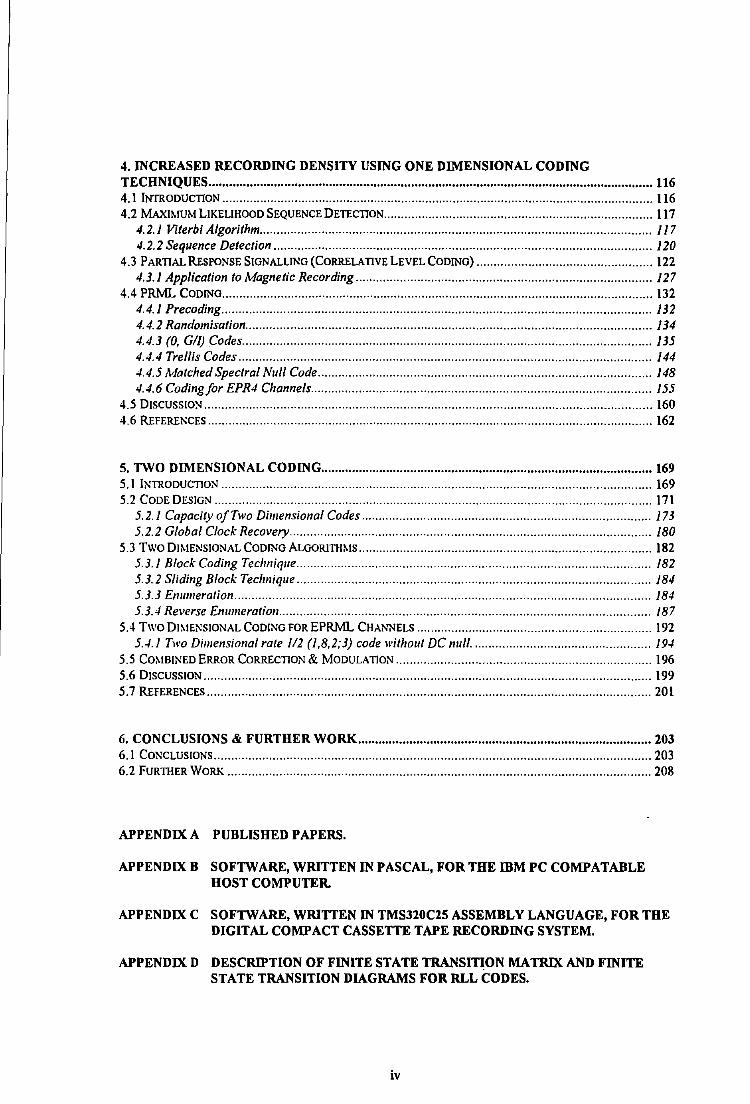
4. INCREASED RECORDING DENSITY USING ONE DIMENSIONAL CODING TECHNIQUES ................................................................................................................................. 116 4.1 INTRODUCTION .........................................................................................•................................... 116

4.2 MAxi~fiJM LIKELIHOOD SEQUENCE DETECTION .......................................•...................................... 117

4. 2.1 Viterbi Algorithm .................................................................................................................. 1 J 7 4.2.2 Sequence Detection .............................................................................................................. 120

4.3 PARTIAL RESPONSE SIGNALLING (CORRELATIVE LEVEL CODING) ................................................... 122

4.3. 1 Application to Magnetic Recording ...................................................................................... 127 4.4 PJUviL CODING .....................................................................................................••...................... 132

4.4.1 Precoding ............................................................................................................................. 132 4.4.2 Randomisation ...................................................................................................................... 134 4.4.3 (0, GIJ) Codes ....................................................................................................................... 135 4.4.4 Trellis Codes ........................................................................................................................ 144 4.4.5 Matched Spectral Null Code ................................................................................................. 148 4.4.6 Coding for EPR4 Channels ................................................................................................... 155

4.5 DISCUSSION .................................................................................................................................. 160

4.6 REFERENCES ................................................................................................................................. 162

5. TWO DII\1ENSIONAL CODING ................................................................................................ 169 5.1 INTRODUCTION ............................................................................................................................. 169

5.2 CODE DESIGN ............................................................................................................................... 171

5.2.1 CapacityofTwo Dimensional Codes .................................................................................... 173 5.2.2 Global Clock Recovery ......................................................................................................... 180

5.3 TWO DIMENSIONAL CODING ALGORITIIMS ..................................................................................... 182

5.3. 1 Block Coding Technique ....................................................................................................... 182 5.3. 2 Sliding Block Technique ....................................................................................................... 184 5.3.3 Enumeration ......................................................................................................................... /84 5.3.4 Reverse Enumeration ............................................................................................................ /87

5.4 Two DI~IENSIONAL CODING FOR EPJUv!L CHANNELS .................................................................... 192

5.4./ Two Dimensional rate /12 (/,8,2;3) code without DC null .................................................... /94 5.5 COMBINED ERROR CoRRECTION & MODULATION .......................................................................... 196

5.6 DISCUSSION .................................................................................................................................. 199

5.7 REFERENCES ..........................................................................................•...................................... 201

6. CONCLUSIONS & FURTHER WORK ..................................................................................... 203 6.1 CONCLUSIONS ............................................................................................................................... 203

6.2 FURTHER WORK ........................................................................................................................... 208

APPENDIX A PUBLISHED PAPERS.

APPENDIX 8 SOFTWARE, WRITTEN IN PASCAL, FOR THE mM PC COMPATABLE HOST COMPUTER.

APPENDIX C SOFTWARE, WRITIEN IN TMS320C25 ASSEMBLY LANGUAGE, FOR THE DIGITAL COMPACT CASSETTE TAPE RECORDING SYSTEM.

APPENDIX D DESCRIPTION OF FINITE STATE TRANSITION MATRIX AND FINITE STATE TRANSITION DIAGRAMS FOR RLL CODES.

iv

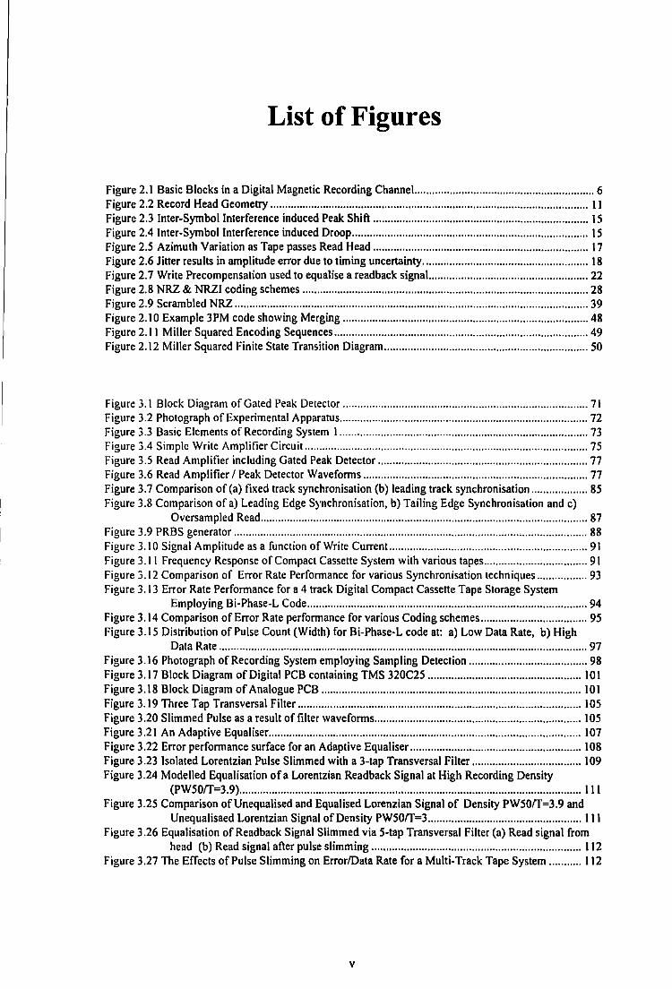
List of Figures

Figure 2.1 Basic Blocks in a Digital Magnetic Recording Channel... .......................................................... 6 Figure 2.2 Record Head Geometry ............................................................................................................ 11 Figure 2.3 Inter-Symbol Interference induced Peak Shift ......................................................................... 15 Figure 2.4 Inter-Symbol Interference induced Droop ................................................................................ 15 Figure 2.5 Azimuth Variation as Tape passes Read Head ......................................................................... 17 Figure 2.6 Jitter results in amplitude error due to timing uncertainty ........................................................ 18 Figure 2. 7 Write Precompensation used to equalise a readback signal... ................................................... 22 Figure 2.8 NRZ & NRZI coding schemes ................................................................................................. 28 Figure 2.9 Scrambled NRZ ........................................................................................................................ 39 Figure 2.10 Example 3PM code showing Merging ................................................................................... 48 Figure 2.11 Miller Squared Encoding Sequences ...................................................................................... 49 Figure 2.12 Miller Squared Finite State Transition Diagram ..................................................................... 50

Figure 3.1 Block Diagram of Gated Peak Detector ................................................................................... 71 Figure 3.2 Photograph of Experimental Apparatus .................................................................................... 72 Figure 3.3 Basic Elements of Recording System ) .................................................................................... 73 Figure 3.4 Simple Write Amplifier Circuit ................................................................................................ 75 Figure 3.5 Read Amplifier including Gated Peak Detector ....................................................................... 77 Figure 3.6 Read Amplifier I Peak Detector Waveforms ............................................................................ 77 Figure 3. 7 Comparison of (a) fixed track synchronisation (b) leading track synchronisation ................... 85 Figure 3.8 Comparison of a) Leading Edge Synchronisation, b) Tailing Edge Synchronisation and c)

Oversampled Read ............................................................................................................... 87 Figure 3.9 PRBS generator ........................................................................................................................ 88 Figure 3.10 Signal Amplitude as a function of Write Current. .................................................................. 91 Figure 3.11 Frequency Response of Compact Cassette System with various tapes ................................... 91 Figure 3.12 Comparison of Error Rate Performance for various Synchronisation techniques ................. 93 Figure 3.13 Error Rate Performance for a 4 track Digital Compact Cassette Tape Storage System

Employing Bi-Phase-L Code ............................................................................................... 94 Figure 3.14 Comparison of Error Rate performance for various Coding schemes .................................... 95 Figure 3.15 Distribution of Pulse Count (Width) for Bi-Phase-L code at: a) Low Data Rate, b) High

Data Rate ............................................................................................................................. 97 Figure 3.16 Photograph of Recording System employing Sampling Detection ........................................ 98 Figure 3.17 Block Diagram of Digital PCB containing TMS 320C25 .................................................... 101 Figure 3.18 Block Diagram of Analogue PCB ........................................................................................ 101 Figure 3.19 Three Tap Transversal Filter ................................................................................................ I 05 Figure 3.20 Slimmed Pulse as a result of filter waveforms ...................................................................... 105 Figure 3.21 An Adaptive Equaliser .......................................................................................................... I 07 Figure 3.22 Error performance surface for an Adaptive Equaliser .......................................................... 108 Figure 3.23 Isolated Lorentzian Pulse Slimmed with a 3-tap Transversal Filter ..................................... 109 Figure 3.24 Modelled Equalisation of a Lorentzian Readback Signal at High Recording Density

(PW50/T=3.9) .................................................................................................................... Ill Figure 3.25 Comparison ofUnequalised and Equalised Lorenzian Signal of Density PW50/T=3.9 and

Unequalisaed Lorentzian Signal of Density PW50/T=3 .................................................... Ill Figure 3.26 Equalisation of Readback Signal Slimmed via 5-tap Transversal Filter (a) Read signal from

head (b) Read signal after pulse slimming ....................................................................... 112 Figure 3.27 The Effects of Pulse Slimming on Error/Data Rate for a Multi-Track Tape System ........... 112

V

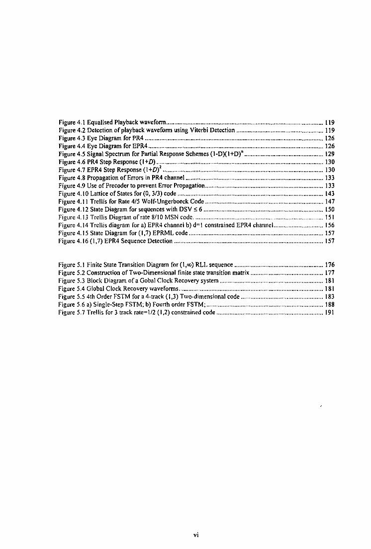
Figure 4 .I Equalised Playback wavefonn ................................................................................................ 119 Figure 4.2 Detection of playback wavefonn using Viterbi Detection ..................................................... 119 Figure 4.3 Eye Diagram for PR4 ............................................................................................................. 126 Figure 4.4 Eye Diagram for EPR4 ........................................................................................................... 126 Figure 4.5 Signal Spectrum for Partial Response Schemes (1-D)(I +D)" ................................................ 129 Figure 4.6 PR4 Step Response (I +D) ...................................................................................................... 130 Figure 4.7 EPR4 Step Response (l+D)2

.................................................................................................. 130 Figure 4.8 Propagation of Errors in PR4 channel .................................................................................... 133 Figure 4.9 Use ofPrecoder to prevent Error Propagation ........................................................................ 133 Figure 4.10 Lattice of States for (0, 3/3) code ......................................................................................... 143 Figure 4.11 Trellis for Rate 4/5 Wolf-Ungerboeck Code ........................................................................ 147 Figure 4.12 State Diagram for sequences with DSV::;; 6 ......................................................................... 150 Figure 4.13 Trellis Diagram of rate 8/10 MSN code ............................................................................... 1 S 1 Figure 4.14 Trellis diagram for a) EPR4 channel b) d= I constrained EPR4 channel .............................. 156 Figure 4.15 State Diagram for (I, 7) EPRML code .................................................................................. 157 Figure 4.16 (1,7) EPR4 Sequence Detection ........................................................................................... 157

Figure 5.1 Finite State Transition Diagram for (I,oo) RLL sequence ...................................................... 176 Figure 5.2 Construction of Two-Dimensional finite state transition matrix ............................................ 177 Figure 5.3 Block Diagram of a Gobal Clock Recovery system ............................................................... 181 Figure 5.4 Global Clock Recovery wavefonns ........................................................................................ 181 Figure 5.5 4th Order FSTM for a 4-track (1,3) Two-dimensional code .................................................. 183 Figure 5.6 a) Single-Step FSTM; b) Fourth order FSTM; ....................................................................... 188 Figure 5.7 Trellis for 3 track rate=I/2 (1,2) constrained code ................................................................. 191

vi

Acknowledgement

I would like to express my gratitude to all those people and organisations who have been associated with this project, in particular:

My supervisors Dr. T. Donnelly (Director of Studies) and Professor D. J. Mapps of the School of Electronic, Communication and Electrical Engineering, for their constant support, encouragement, guidance and friendship throughout the project.

Dr Neil Darragh of the C.R.I.S.T. research group, who, through many interesting and lively discussions has significantly clarified and broadened my knowledge in this area.

Mr. Paul Smithson of the School of Electronic, Communication and Electrical Engineering for his help on clock recovery and interfacing to the TMS320C25 digital

signal processor.

My friends and colleagues at the University of Plymouth whose comradeship and encouragement together with innumerable discussions have aided my work

immeasurably.

All the technical staff within the School of Electronic, Communication and Electrical

Engineering for their practical help.

And, not least of all, to my Parents and my wife Moira, without whose unlimited support, patience, love and understanding this work would not have been possible.

vii

Declaration

I declare that this thesis is the result of my own investigation, and is not submitted in

candidature for the award of any other degree. At no time during the registration for the

degree of Doctor of Philosophy has the author been registered for any other University

award.

During the research programme I undertook a course of advanced studies. These

included the extensive reading of literature relevant to the research project, and

attendance of international conferences and seminars on signal processing, coding and

magnetic recording.

Papers were presented at the Euromicro'92 Conference, Paris, France, 1992 and at the

IEEE International Magnetics Conference (Interrnag '94), Albuquerque, New Mexico

1994.

Paul James Davey

D•re#

viii

rir dedicate this thesis .to mY'childi'ell

rChristine and l\1ichaelil);rvey

and ,to the memory of: my gtanciparellts

Rose & Jim rPhilllps

,ix

CHAPTER!

Introduction

The advent of the information age brings an enormous demand for storage of digital

data, along with the demands for processing and transmission of such data. For each of

the past three decades the capacity of magnetic storage devices has risen by an order of

magnitude. Most of this increased storage density has resulted from improvements in

the part of the system we call "tlte c/rmmel", which includes the storage medium itself,

the read/write heads with associated electronics, and the positioning of these heads.

If we restrict attention to linear density gains, the progress due to advances in signal

processing and coding technology has also made a significant improvement to the linear

density achievable with a typical set of recording components. However, instead of

utilising modern modulation and coding methods that would yield performance closer to

the channel capacity, the design engineers for storage systems have taken the alternative

approach of increasing the channel capacity itself. This development has resulted in the

utilised channel capacity being well below that which is theoretically possible.

Magnetic recording is by far the most popular technique for storing information, in

particular magnetic tape has become the predominant means for mass storage of both

digital and analogue data. The principal advantage of magnetic tape as a data storage

medium is it can store large amounts of information in a relatively small amount of

space, and at low cost per bit. In spite of the great progress in optical and electronic

technology, it seems that no viable substitution for magnetic memory, tape or disk, for

mass storage will become available in the near future. Therefore, the future trend will be

to improve the capacity of current recording techniques through the application of

advanced signal processing.

Modern communication theory has played a major role in increasing the efficiency and

reliability of communication systems. The aim of this research is to achieve analogous

increase in reliability for the storage and retrieval of digital data in magnetic recording

systems. More specifically, here the aim is to increase the capacity or packing density

of a digital magnetic storage system by increasing the amount of data that can be stored

in a unit area of magnetic media. This can be achieved by increasing linear density

and/or by increasing the track density. All of this must be accomplished without

sacrificing the reliability of the retrieved data.

Recent work at the University of Plymouth has demonstrated the effectiveness of

employing a programmable device in the data channel of a recording system. By

harnessing the flexibility of a microprocessor in an adaptive manner excellent error/data

rate performance has been achieved using a standard cassette mechanism.

It is therefore proposed to extend this work and examine, in part, the application of

advanced digital signal processing and, in particular, channel coding schemes to a

digital magnetic tape recording system as a means of continuing the increase in density.

Techniques are investigated that can more efficiently utilise the available spatial

bandwidth of the magnetic recording channel, leading to the desired density increases. A

further aim is also to offset the mechanical vagaries of a low-cost tape transport and

tape, such as the compact-cassette format, by intelligent software algorithms. The

2

problem of low signal to noise ratios and high error rates can be alleviated by employing

more sophisticated coding schemes that will exploit the multiple-track capabilities of

such a system.

Chapter 2 describes the basic elements of a digital magnetic recording channel. The

chapter proceeds to describe the sources of error present in the recording channel and

some channel coding and equalisation techniques that have been applied to overcome

them. Important properties of modulation codes are discussed, in particular run-length

limited, and charge constrained modulation codes and their application to the magnetic

recording channel. A systematic review is presented of an assortment of various codes

that have been adopted in practical storage systems, some of which were also

implemented by the author in the peak detect system. The chapter concludes with a

description of some alternative modulation coding techniques that include error

correction capabilities and multi-level recording.

Chapter 3 describes the initial hardware and software employed in the first stage of the

investigation. This system is categorised by the type of detection that was implemented,

namely peak detection. The experimental procedure and results pertaining to this system

are also given. The chapter continues to discuss the application of a second digital

magnetic recording system designed and constructed by the author. This recording

system differs from the previous design in that it incorporates a sampling detection

system that periodically samples the amplitude of the readback signal and converts the

result from the analogue to digital domain, after suitable amplification and filtering.

3

Finally an equalisation technique employing a digital filter to pulse-slim the readback

signal and increase the data rate for a given error rate is also described.

Chapter 4 discusses the application of advanced signal processing techniques, such as

Partial Response Signalling and Maximum Likelihood Sequence Detection as a means

to further increase linear recording density. The code constraints and several coding

techniques, including trellis codes and Matched Spectral Null codes, pertaining to such

a system are described in some detail.

Chapter 5 describes a new class of modulation codes that exploits the two-dimensional

properties of multi-track digital magnetic recording systems to provide increased area!

storage density. Techniques for constructing multi-track codes are discussed and a new

technique for implementing a two-dimensional code is presented. The chapter ends by

discussing the application of a new two-dimensional code to a multi-track system

employing extended class IV partial response and maximum likelihood detection.

Finally the author's conclusions are presented m Chapter 6, together with areas of

further work.

4

CHAPTER2

Background to the Investigation

2.1 Magnetic Recording of Digital Information

The magnetic recording process is based on the interaction between the magnetic

storage medium and the magnetic head; usually the two are moving with respect to each

other. In the recording process the head magnetises the medium, whilst during replay

the head 1 generates an induced voltage reflecting the rate of change of magnetisation

recorded on the surface.

The magnetic recording channel can be viewed as a communication channel that has a

band-pass frequency response which suffers from both amplitude and timing instability

and is non-linear due to the hysteresis exhibited by the magnetic medium. Transmission

of d.c. is prevented since the read head output voltage is proportional to the derivative of

the head flux. The low frequency limit is directly related to the overall physical

dimensions of the read head, whereas the high frequency response is limited by the read

head gap null, the inductance of the read head and the existence of spacing losses. At

1 This discussion assumes an inductive head. Magneto-Resistive heads produce a signal proportional to

the flux rather than the rate of change of flux.

5

low and medium frequency a recording channel may be rendered linear by the use of

a.c. bias.

2.1.1 Digital Recording Theory

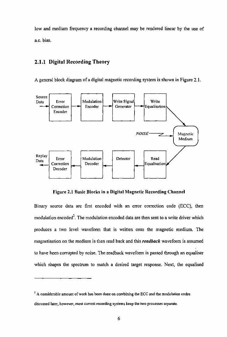
A general block diagram of a digital magnetic recording system is shown in Figure 2.1.

urce So D ala -

play Re D ala ~

Error Modulation Write Signal Write Correction - Encoder ~ G""'"'' ~ Eq~U.,tioo ~

Encoder

, ....,

NOISE Magnetic Medium

' ./

Error Modulation Detector ·~ / Correction I-- Decoder I-- I-- Equalisation Decoder

Figure 2.1 Basic Blocks in a Digital Magnetic Recording Channel

Binary source data are first encoded with an error correction code (ECC), then

modulation encoded2• The modulation encoded data are then sent to a write driver which

produces a two level waveform that is written onto the magnetic medium. The

magnetisation on the medium is then read back and this readback waveform is assumed

to have been corrupted by noise. The readback waveform is passed through an equaliser

which shapes the spectrum to match a desired target response. Next, the equalised

2 A considerable amount of work has been done on combining the ECC and the modulation codes

discussed later, however, most current recording systems keep the two processes separate.

6

waveform is sent to the detector which produces an estimate of the channel data. The

estimate is then decoded by the modulation decoder and finally an error correction

decoder is employed to recover any errors.

A multiple-track recording system consists of two or more basic systems in parallel,

each track usually working independently of the others. However, the multi-track

recording system used throughout this thesis employs the operation of several tracks

simultaneously. It will be discussed later in this dissertation how parallel channels offer

distinct advantages, in terms of recording density and clock recovery, over conventional

serial operation.

Channel Capacity

Shannon [1] proved that the channel capacity C, could be calculated such that if the

maximum information rate R, at which information can be transmitted is less than C,

data can be sent error free through a noisy channel. Channel capacity C is defined as

C (bits/second) = B log2 (1 + SNR) eqn{ 1}

where

B = channel Bandwidth (Hz),

SNR = Signal to Noise Ratio = Signal power (watts) I Noise power (watts).

This classic law assumes Additive White Gaussian Noise (A WGN), i.e. the noise is

additive, covers all frequencies and has a Gaussian distribution.

This shows that the bandwidth of a channel and the signal to noise ratio (SNR) may be

traded off against each other in achieving the desired capacity.

7

Mallinson [2] shows that the SNR for a tape of width W may be approximated as

eqn{2}

where

Amin = minimum recorded wavelength,

NP = number of magnetic particles per unit volume.

Therefore if the width of the tape is divided into y tracks (ignoring guard-bands) the

SNR of each track is reduced by l !y, giving a total channel capacity of

Cy = y.B.log2(l+SNR/y). eqn{3}

Therefore, from equation {3 }the capacity will increase linearly with the number of

tracks as will the area! packing density. However, this is at the expense of reduced SNR.

In addition, equation {2} shows that doubling the number of tracks reduces the SNR by

3dB, whilst halving the minimum recorded frequency reduces the SNR by 6dB. Hence,

it seems beneficial to have a multi-track system operating at a reduced data rate.

However, as track widths narrow substantially other sources of noise such as crosstalk

and dropouts become more relevant.

Systems that approach the Shannon bound usually incorporate error correction coding,

where enough redundancy has been added to the transmitted signal to allow the decoder

to detect and correct any errors that might occur.

One of the problems which makes research in signal processing for magnetic channels

difficult is that entirely satisfactory models have not been found. The mathematical

models which are used today range from finite difference methods requiring super­

computers to linear systems approaches running on personal computers. The models

8

which accurately capture the essence of a magnetic recording system tend to be far too

complex for signal processing applications, whilst the models that are simple enough for

use in signal-processing algorithms generally have extreme restrictions on the operating

conditions in which they are valid. In addition the noise which one must deal with is

non-stationary and not very well characterised and in some cases, such as thin -film

media, is data dependent.

Therefore, in this research we have tried to limit channel modelling to a minimum,

using real or sampled signals whenever possible. However, this is not always

convenient for predicting results.

Pulse Superpositio11

Linear pulse superposition [3] applied to magnetic recording states that the voltage

waveform produced by a series of flux reversals is the algebraic sum of a series of

isolated pulses, centred on the flux reversals.

Expressed mathematically, the combination of a number x, of isolated pulses p(l),

separated by T/2 is

where T= 1/data rate.

T e(l)= L(-l)'.p(t+x.-)

X 2 eqn{4}

Once the shape of the isolated pulse p(t), has been determined, the voltage of the replay

signal can be generated by combining pulses with the appropriate spacing for any

recorded data sequence at any desired packing density.

9

Non-linear Distortion

The principle of linear superposition is very accurate for systems operating at low

densities and at low data rates. However, it has been well documented that the linear

superposition model begins to break down as the spatial separation between recorded

transitions becomes smaller [4,5). The most common form of non-linear distortion is

non-linear bit shift or non-linear inter-symbol interference. Non-linear bit shift is due to

the magnetic field interaction between adjacent recorded transitions and the head field

as they are being recorded. The non-linear interaction depends upon the previously

written data and as such can usually be precomputed and compensated on the write side

\\·ith \\'fite-precompensation (discussed later).

As the spatial density of the recording system is further increased other non-linear

distortions can occur such as partial erasure [6). These non-linearities are beyond the

scope of this investigation and as such are neglected.

Lorentzian Model

The accuracy of modelling the channel using pulse superposition is dependent on the

shape and width of the isolated pulse used. A simple and frequently used expression to

represent the replay signal is given by the Lorentzian pulse described in Equation { 5}

where

p(t)=--­I +(-t-)2

Pffso

PW50 is the pulse width at half (50%) height.

10

eqn{S}

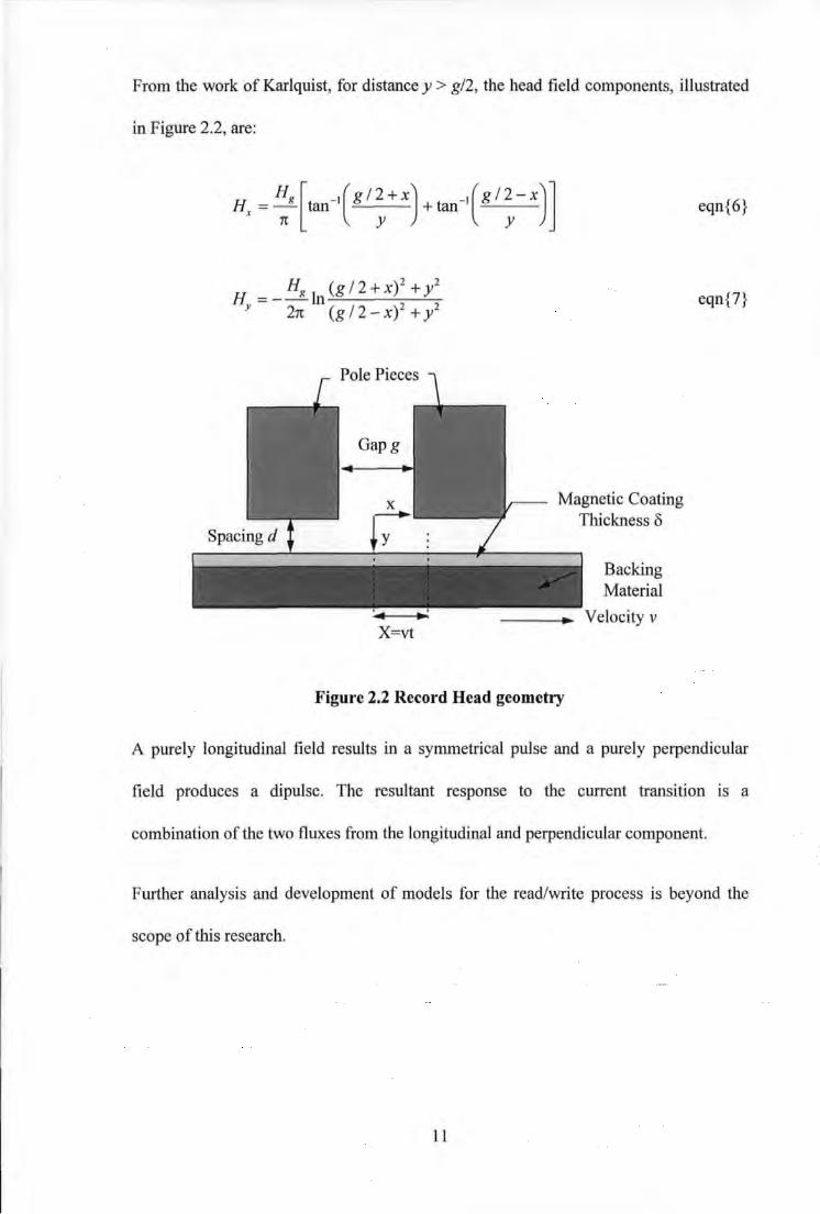
From the work of Karlquist, for distance y > g/2, the head field components, illustrated

in Figure 2.2, are:

H Hg [ _1(g/2+x) _,(g/2-x)] x = - tan +tan

1t y y

Magnetic Coating Thickness 8

Backing Material

Velocity v

Figure 2.2 Record Head geometry

eqn{6}

eqn{7}

A purely longitudinal field results in a symmetrical pulse and a purely perpendicular

field produces a dipulse. The resultant response to the current transition IS a

combination of the two fluxes from the longitudinal and perpendicular component.

Further analysis and development of models for the read/write process is beyond the

scope of this research.

11

2.1.2 Practical Limitations

The recording channel differs from most communication systems in a number of

respects. Reliability requirements are usually much higher for magnetic recording

systems. For instance, an error rate of 10"12 or less is not uncommon, also signal power

is limited and can not be increased with respect to noise. It is therefore essential to

completely define and understand all the error causing mechanisms.

Noise

Many communications' systems have only a single type of noise, whereas in magnetic

recording channels there are several major sources of error:

a) media noise,

b) electronics noise,

c) read/write noise.

Despite limited amounts of available quantitative data, the behaviour of the noise can be

roughly described as follows.

Media noise is due to the manufacturing irregularities and to weak recorded tracking

information. Media noise may contain a spike component, due to impurities, which

results in such a large noise level that no data bits can be written at those geographic

locations on the magnetic surface. The noise also contains a continuous component,

which may be due to the non-uniformity of the ferromagnetic material.

All components with resistance generate noise according to their temperature, the

electronics and more importantly the read/write head are no exception. Over the normal

12

operational temperature range this noise is more or less constant. The reading and

writing noise contain an electrical component of uncertain spectrum, possibly white, and

a mechanical component of coloured spectrum, resulting from the variations in distance

between the head, the medium and neighbouring head/medium signals. In general, for a

given recording on tape, a better signal to noise ratio will be obtained by moving the

tape relative to the head at a higher speed, since the head noise is constant and the signal

induced is proportional to speed. This is one advantage that rotary head recorders have

over stationary head recorders.

Inter-Symbol Interference

Due to the finite gap of the replay head, increasing the density of recorded data stored

on the magnetic medium causes closely spaced magnetic transitions to interfere with

one another. This phenomenon, known as Inter-Symbol Interference (ISI) results in

peak shift distortion, also known as pulse crowding, and reduction in signal amplitude

causing timing and detection errors.

The recording density effectively specifies a length of track or time interval in which

each flux reversal is contained. This is termed the bit-cell or bit interval. In digital

recording, a large number of output pulse patterns arise. At low densities each pulse is

individually resolved. With higher densities the dispersivity of the channel causes each

flux reversal to spill over from its cell into the cells of its neighbours. In this way the

flux reversals or symbols interact in such a way as to cause distortion.

The adverse effects of ISI are manifested in two ways:-

13

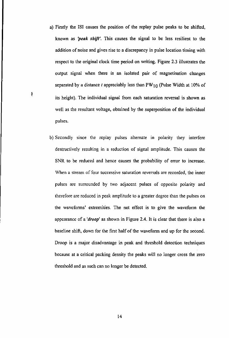
a) Firstly the ISI causes the position of the replay pulse peaks to be shifted,

known as 'peak shift'. This causes the signal to be less resilient to the

addition of noise and gives rise to a discrepancy in pulse location timing with

respect to the original clock time period on writing. Figure 2.3 illustrates the

output signal when there is an isolated pair of magnetisation changes

separated by a distance t appreciably less than PW 10 (Pulse Width at I 0% of

its height). The individual signal from each saturation reversal is shown as

well as the resultant voltage, obtained by the superposition of the individual

pulses.

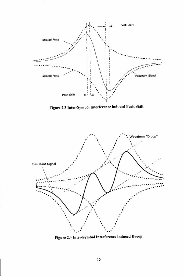
b) Secondly smce the replay pulses alternate in polarity they interfere

destructively resulting in a reduction of signal amplitude. This causes the

SNR to be reduced and hence causes the probability of error to increase.

When a stream of four successive saturation reversals are recorded, the inner

pulses are surrounded by two adjacent pulses of opposite polarity and

therefore are reduced in peak amplitude to a greater degree than the pulses on

the waveforms' extremities. The net effect is to give the waveform the

appearance of a 'droop' as shown in Figure 2.4. It is clear that there is also a

baseline shift, down for the first half of the waveform and up for the second.

Droop is a major disadvantage in peak and threshold detection techniques

because at a critical packing density the peaks will no longer cross the zero

threshold and as such can no longer be detected.

14

'

Isolated Pulse

' ---. ' '

~-- Peak Shift

. --. ·-- ..... -.- --·--··--· ......... __ ............ -....

;:>-· .... . ·;-'I Isolated Pulse

' ' ' .

' Peak Shift ~--· I '

--- ', I '•' ' ' ' '•"' I I

Figure 2.3 Inter-Symbol Interference induced Peak Shift

-- "- 11 '

• . Waveform "Droop" , \ ' ' • • /

' ' • \

• ' ,/

' ' • / ' • ' ' ' \

• I ' . • •· / • I'· ' /

Resultant Signal . /\ I,,. \ /

\ • -~ \ -J . , . -.. -· ~,.....,. __ -· -·-··' . .... Ill- ........

·:: .... \······-·· / /

/ / ········-. -.-. -~-. ... '. ~'~ ·-···· ----· .. -...... ' .. .,• ... -. .. ., .

• _ ... • •

~ • • • ' • ' • • I

I ' • ' ' •

' ' I ' \

, ' '

' ' • . . , ... -· Figure 2.4 Inter-Symbol Interference induced Droop

IS

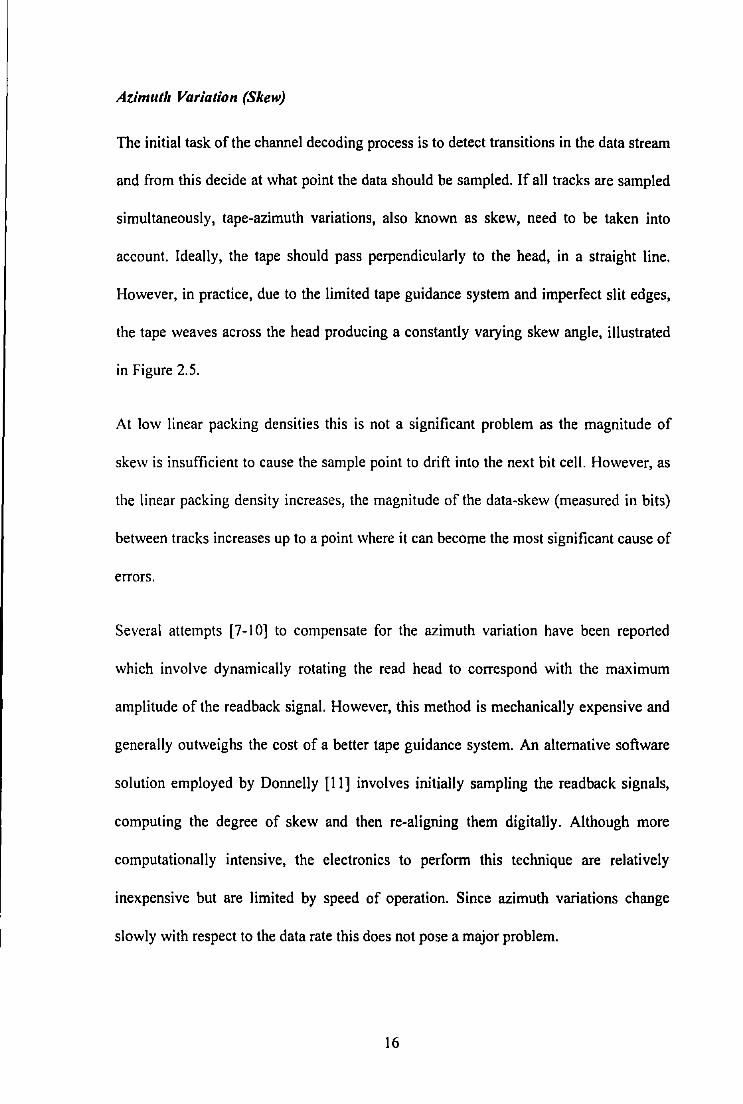
Azimut/1 Variation (Skew)

The initial task of the channel decoding process is to detect transitions in the data stream

and from this decide at what point the data should be sampled. If all tracks are sampled

simultaneously, tape-azimuth variations, also known as skew, need to be taken into

account. Ideally, the tape should pass perpendicularly to the head, in a straight line.

However, in practice, due to the limited tape guidance system and imperfect slit edges,

the tape weaves across the head producing a constantly varying skew angle, illustrated

in Figure 2.5.

At low linear packing densities this is not a significant problem as the magnitude of

skew is insufficient to cause the sample point to drift into the next bit cell. However, as

the linear packing density increases, the magnitude of the data-skew (measured in bits)

between tracks increases up to a point where it can become the most significant cause of

errors.

Several attempts [7 -I 0] to compensate for the azimuth variation have been reported

which involve dynamically rotating the read head to correspond with the maximum

amplitude of the read back signal. However, this method is mechanically expensive and

generally outweighs the cost of a better tape guidance system. An alternative software

solution employed by Donnelly [11] involves initially sampling the readback signals,

computing the degree of skew and then re-aligning them digitally. Although more

computationally intensive, the electronics to perform this technique are relatively

inexpensive but are limited by speed of operation. Since azimuth variations change

slowly with respect to the data rate this does not pose a major problem.

16

MAG~E:TIC TAPE: I

Face of Record/Playback Head I

liZJ

Displacemcnl belwecn Tracks l i.: 4

______ , ,---

Skew Angle

Figure 2.5 Azimuth Variation as Tape passes Read Head

Jitter

In analogue audio equipment timing instability of the readback waveform gives rise to

wow and flutter: in digital recording this term is referred to as }iller. In the main j itter is

largely due to head-tape velocity variation. Magnetic tape transports are designed to

provide a linear motion of the tape with as little variation as possible. However, in

practice the combination of mechanical and electrical tolerances for the tape drive in

conjunction with environmental factors such as vibration, etc., result in velocity

variations exceeding the specified tolerance [ 12].

Static friction (stiction) between the in-contact head and slow moving tape can cause

micro velocity changes which are excited by the flexibility and surface irregularities of

the tape. Together these are also responsible for the most significant amount of jitter.

17

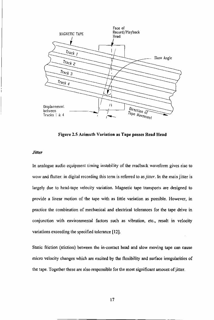
Figure 2.6 illustrates how jitter causes uncertainty about the signal voltage relative to a

stable time reference for a signal with a finite rate of change of voltage; this has the

same effect as noise. Since jitter is directly proportional to the rate of change of voltage

in the readback signal the degree to which it affects the error rate increases with

frequency. This introduces an important channel code parameter, the jitter margin Two

also termed window margin or phase margin, that determines the tolerance in locating a

transition in a bit cell. It is defined as the permitted range of time over which a transition

can still be received correctly, divided by the data bit cell period T. In general the larger

the value of r .. the better since it has the effect of reducing peak shift distortion.

Voltage Error 'Jitter noise'

__..: 14- Timing uncertainty I I

Figure 2.6 Jitter results in amplitude error due to timing uncertainty.

In a sampling system, a finite amount of variation in the sampling clock can lead to

timing fitter. This has to be carefully controlled since this has the potential to cause

more catastrophic errors than in the previous type of jitter. Since the theory underlying

the correct operation of most digital signal processing techniques, such as filtering etc.,

relies on samples at regular intervals.

18

Dropouts

Many shallow drops in the envelope of the readback signal can be observed in high

density digital magnetic recording. Asperities and discontinuities in the recording

medium cause hard dropouts which have a drastic effect on the recorded signal,

however these are minimised by modem medium manufacturing techniques. More

common are losses in level caused mainly by instantaneous increases in the separation

between the tape and the head due to surface roughness of the tape and debris such as

dust and oxidised particles. These are termed soft dropouts. Increase in separation

causes not only a drop in the envelope but also a loss of amplitude in the higher

frequencies of the read back signal. Perry et al. [ 13] have demonstrated how a

microprocessor based system can be used to characterise the effect of dropouts for a

high density digital magnetic tape system. Meeks [14] further describes how an

appropriate error correction strategy can be selected once the dropout characteristics are

determined.

Crosstalk

To increase track density care must be taken that the tracks are not so closely spaced

that serious pickup leakage interference arises from adjacent recorded tracks. Since the

amount of leakage increases with the wavelength of the recorded signal, (similar to the

separation loss), the leakage can become pronounced potentially resulting in problems at

low frequencies. This type of noise is termed crosstalk and can be considered as similar

to the influence of Gaussian noise, since the leakage power is restricted to lie within the

low frequency range and the random data signals recorded on the tracks are presumed to

have no correlation with each other. Hence channel codes that have little or no low

frequency response are less prone to crosstalk induced errors.

19

2.2 Channel Equalisation

To enhance the perfonnance of the magnetic recording channel at high packing densities

appropriate equalisation techniques must be applied to match the frequency and phase

response of the recording channel to that of the recorded signal. Equalisation is the

process that modifies the transfer function of the analogue channel to provide more

reliable data detection by compensating for the channel distortions such as ISI and peak

shift. However, the improvement in the channel transfer function is usually

accompanied by a degradation in signal to noise ratio, resulting from boosting the high

frequencies where there is little signal and much noise. Therefore, although any degree

of equalisation can be theoretically applied, the equaliser design will usually be a

compromise between the required transfer function and the resultant loss in SNR due to

equalisation.

The choice of equalisation depends upon the following:

a) the amount of inter-symbol interference to be compensated,

b) the modulation code,

c) the detection technique used,

d) the signal to noise ratio,

e) the noise spectrum shape.

Channel equalisation may be implemented either prior to the recording process, in

which case it is referred to as write equalisation or write precompensation, or during the

replay process where it is tenned read or post equalisation or simply just equalisation.

20

2.2.1 Write Equalisation

Write equalisation attempts to modify the spectral components of the signal to be

recorded or written to match the frequency response of the channel. The principle

benefit of write equalisation is that all the signal conditioning is performed before noise

is introduced into the system, hence reducing noise in the readback signal relative to

post-equalisation.

However, in practice it is difficult to provide correct equalisation using a write equaliser

alone since the channel response is constantly varying due to tape surface asperities,

substrate irregularities and the intimacy of the head contact and wear. These variations

attenuate the high frequencies much more than the low frequencies which undermines

any predicted or fixed equalisation scheme.

Write equalisation can be sub-divided into three different techniques:

Amplitude write equalisation

This method varies the amplitude and/or shape of the write current so that it is no longer

a binary signal. Jacoby [15] suggested a cosine equaliser, which is sometimes used for

read equalisation, to shape the write current. This technique is not popular due to the

need for complex write-side electronics.

21

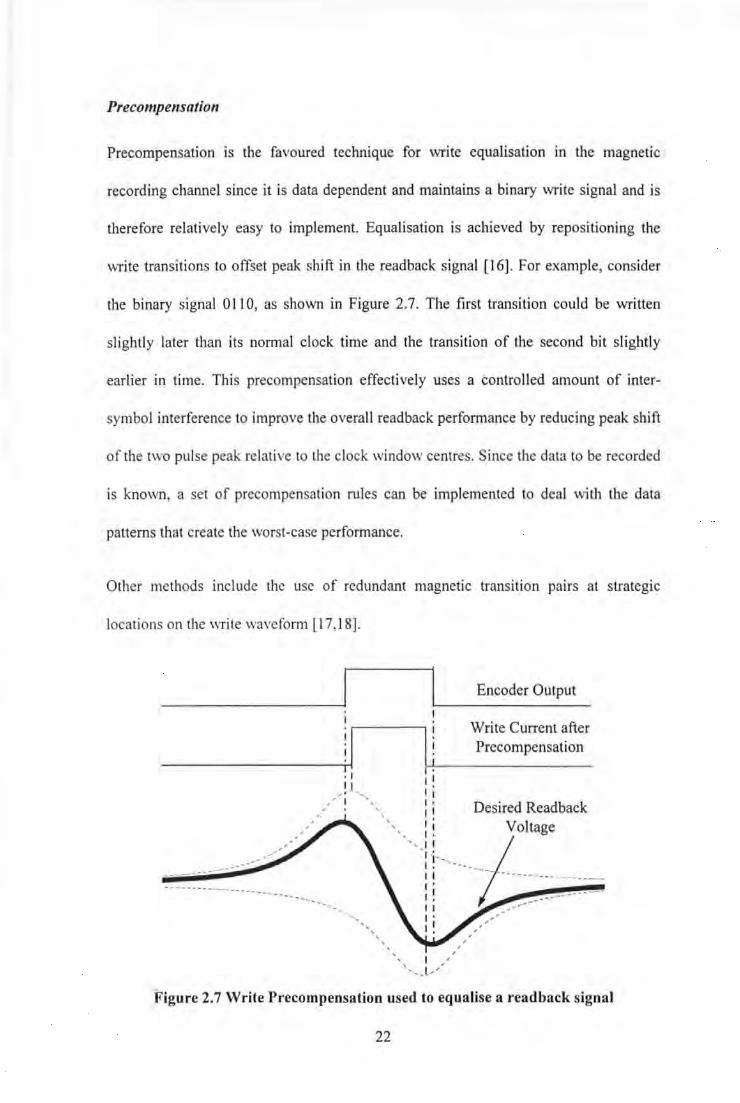
Precompe11satio11

Precompensation is the favoured technique for write equalisation in the magnetic

recording channel since it is data dependent and maintains a binary write signal and is

therefore relatively easy to implement. Equalisation is achieved by repositioning the

write transitions to offset peak shift in the read back signal [ 16]. For example, consider

the binary signal 0110, as shown in Figure 2. 7. The first transition could be written

slightly later than its normal clock time and the transition of the second bit slightly

earlier in time. This precompensation effectively uses a controlled amount of inter-

symbol interference to improve the overall readback performance by reducing peak sruft

of the two pulse peak relative to the clock window centres. Since the data to be recorded

is known, a set of precompensation rules can be implemented to deal with the data

patterns that create the worst-case performance.

Other methods include the use of redundant magnetic transition pa1rs at strategic

locations on the write waveform [17, 18].

Encoder Output

Write Current after Precompensation

Desired Readback

I , ' ' ...... _L ....... "

Figure 2.7 Write Precompensation used to equalise a readback signal

22

Precoding

Both Tomlinson [19] and Harashima and Miyakawa [20] independently proposed

precoding as a means of equalisation over twenty years ago. This technique employs a

feedback transversal filter whose impulse response is the inverse of the channel and

which can also maintain a binary write signal through the use of modulo-two arithmetic.

This technique although not yet fully utilised in magnetic recording has been used, in

conjunction with Trellis Coded Modulation, with great success for achieving increased

data rates in telephone-line modems [21].

2.2.2 Read Equalisation

This method refers to the use of a linear filter at the output which changes the overall

impulse response of the system before the peak detector.

Since read equalisers operate on the signal after noise has been added by the channel the

noise spectrum is modified as well as the signal. Therefore an improvement in distortion

is usually accompanied by a degradation in signal to noise ratio.

The equaliser increases the bandwidth of the signal by compensating for the loss in high

frequencies produced by the recording channel. The increase in bandwidth results in a

narrower pulse in the time domain, which has the effect of reducing pulse interaction

and hence reduces ISI induced peak shift. However, the amplification of the higher

frequency components of the signal spectrum extends the noise power spectral density

causing an increase in average noise power. Hence, noise induced peak shift is

increased. This trade off between ISI and noise-induced peak shift is the basis of

equaliser design.

23

Pulse Slimming

Pulse slimming is a time domain approach to read equalisation, its purpose being to

create a channel whose isolated transition response is a thinner pulse than that produced

by the unequalised channel. Many different types of pulse-slimming filters have been

used to reduce adjacent pulse interference [22-28].

Jacoby [23] describes one of the more classic equaliser circuits, achieved by a resistor,

inductor, capacitance network which controls signal amplitude and phase separately.

Kameyama [25] described a cosine equaliser, that slimmed an isolated pulse by

approximately 30% when the SNR at the input is 35dB. The basic circuit is composed

of a delay line, an amplitude divider and a differential amplifier. The delay line is

terminated with a matching impedance at the input and is open ended at the output so

that the signal is completely reflected. This causes the incoming and reflected pulse to

add constructively and therefore double in amplitude. For an input signal of f;(t+r) the

output of the equaliser f0 (t) is expressed as

2f;(t )-K( f;(t+t )+f;(t -t)) eqn{8}

where t is the delay and K is the ratio of the amplitude divider.

The resultant transfer function of this equaliser described in the frequency domain is

F(co) =I - K cos (co.t) eqn{9}

hence the name cosine equaliser.

24

2.3 Signal Detection

Whereas there have been significant technology developments in read/write heads,

magnetic media and servo systems, the analogue Peak Detectio11 [29] method of data

recovery has remained largely unchanged for over 25 years.

Data detection in the conventional peak detection magnetic recording channel is

achieved by first differentiating the analogue signal and then processing the

differentiated signal with a zero crossing detector to determine the presence or absence

of a zero crossing event within the detection window. In the absence of noise or other

imperfections the zero crossing of the derivative signal in peak detection occur only at

times corresponding to the clock times at which a transition was written. Enhancements

such as precompensation, Run-Length-Limited codes and more sophisticated detectors

have extended the performance of peak detection systems.

The peak detector has the advantage of being both robust and extremely simple to

implement. However, by its very nature it performs best at low linear densities. The

underlying technique used in all peak detection systems is termed a hard limited

process. The output is determined to be either above or below a decision threshold and

performs lrard decisiotrs on each bit (symbol-by-symbol) coming out of the channel. In

doing so this method of detection looses information about how close the signal is to the

threshold and as such how good the decision was. If the data bits passing through a

channel are independent of one another the performance of the detector is optimum.

However, modulation coding introduces correlation among the bits in a sequence and

therefore a hard-decision detection is not optimum.

25

An optimum detection process for correlated data uses a soft decision algorithm that

decides the result based on past, present and future decisions being above or below a

decision threshold and then gives a measure of "goodness" or confidence that

determines how close the result was to the threshold level.

Therefore, whilst the peak detector has been acceptable in the past in terms of

simplicity, low cost and speed, it has become increasingly apparent that to make more

efficient use of available bandwidth a more sophisticated detection method is required.

Recent attention has focused on sampling detection and an entirely new type of

modulation coding and signal processing, a revolutionary rather than evolutionary

approach. These techniques are described further in chapter 4.

A prime requirement in a digital communication channel employing soft decision

detection IS that the amplitude of the readback signal is periodically sampled.

Historically this has prevented the graduation to digital signal processing due to the high

speed requirements of many storage systems and the high cost of fast silicon. Hence,

only recently, with the introduction of high speed compact mixed digital and analogue

signal processors, such techniques have been made feasible. Conversion from the

analogue to digital domain also permits other advanced DSP techniques to be performed

on the signal such as adaptive equalisation and clock recovery.

26

2.4 Modulation Coding

In coding for a magnetic recording channel using saturation recording, engineers are

presented with overcoming an array of potential problems, some of which are not

clearly understood. As opposed to most communication systems:

(a) timing recovery must be obtained from the modulated data,

(b) the noise is non-white and may have a (pattern dependent) multiplicative

nature,

(c) most detection systems are sub-optimal,

(d) uncertainty in channel characteristics must be tolerated,

(e) inter-symbol interference dominates at high recording densities.

Due to the differentiating nature of the read head, only polarity changes in the magnetic­

medium saturation produce significant energy at the output of the read electronics. As

such, the magnetic channel is often modelled as the linear superposition of these step

responses. Since timing recovery must be obtained from the channel response to the

modulation code all modulation codes require relatively frequent changes in magnetic

saturation.

Two common notations used to designate magnetic modulation codes are Non-Return

to Zero (NRZ) and Non-Return to Zero Increment (NRZI). Actual recording bits

consist of saturation in one direction ( + 1) or in the other ( -1 ). In NRZ notation a charge

in one direction of saturation is referred to as a '1', whilst a charge in the opposing

direction is referred to as a '0'. In NRZI notation a change in direction of saturation is

referred to as a '1' and no change i.e. constant state of saturation is referred to as '0'. In

27

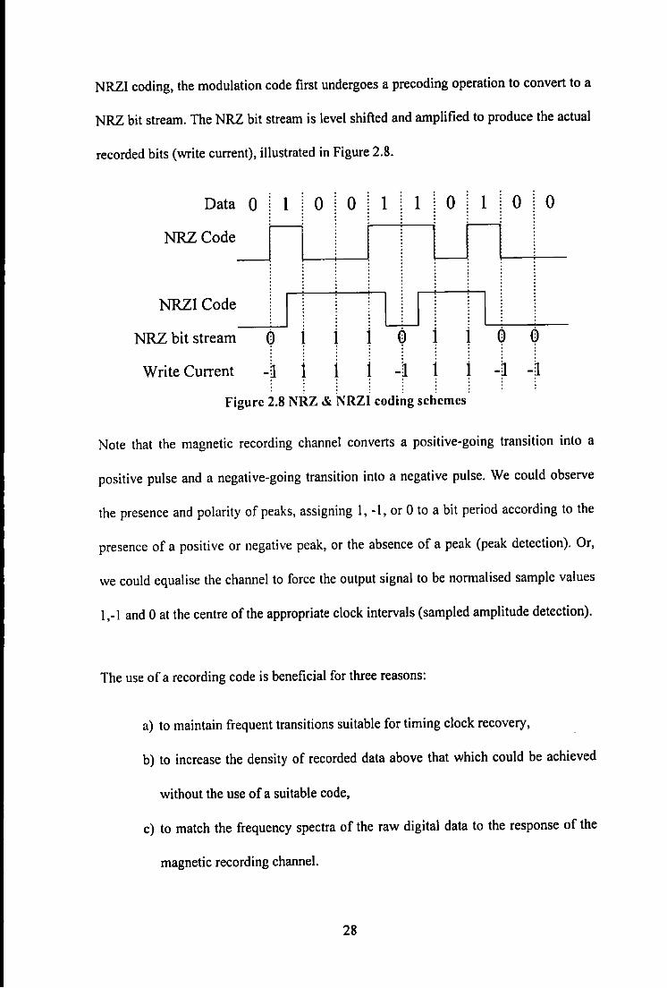
NRZI coding, the modulation code first undergoes a precoding operation to convert to a

NRZ bit stream. The NRZ bit stream is level shifted and amplified to produce the actual

recorded bits (write current), illustrated in Figure 2.8.

Data 0

NRZCode

-

NRZI Code

NRZ bit stream 0 Write Current -1

1 0

i

1

0 1 1

w i i 0

1 1 -1

0

i i

1 1 Figure 2.8 NRZ & NRZI coding schemes

1 0 0

0 0 -1 -1

Note that the magnetic recording channel converts a positive-going transition into a

positive pulse and a negative-going transition into a negative pulse. We could observe

the presence and polarity of peaks, assigning I, -1, or 0 to a bit period according to the

presence of a positive or negative peak, or the absence of a peak (peak detection). Or,

we could equalise the channel to force the output signal to be normalised sample values

1,-1 and 0 at the centre of the appropriate clock intervals (sampled amplitude detection).

The use of a recording code is beneficial for three reasons:

a) to maintain frequent transitions suitable for timing clock recovery,

b) to increase the density of recorded data above that which could be achieved

without the use of a suitable code,

c) to match the frequency spectra of the raw digital data to the response of the

magnetic recording channel.

28

These criteria have lead to the development of several categories of coding techniques:

a) Run Length Limited (RLL) codes,

b) Charge constrained (d.c.-free or d.c.-balanced) block codes,

c) Trellis codes.

The following sections will describe run length limited codes and charge constrained

code since these are most commonly used in conventional peak detection systems.

Chapter 4 will deal with trellis codes since this type of coding is used in channels

employing partial response signalling and maximum likelihood detection.

2.4.1 Run-Length Limited (RLL) Codes

Run-Length-Limited codes are usually classified according to their construction,

implementation or certain desirable properties that they possess. They have found

almost universal application in magnetic and optical disk recording systems [30].

Whatever the notation, the requirement of relatively frequent changes in magnetic

saturation for efficient timing clock recovery is satisfied by limiting the maximum run

of zeros in the code to some integer k. Also, it is often desirable to limit the effects of

ISI and improve performance of the peak detector by imposing a separation between

transitions. This is achieved by imposing a d constraint that relates to the minimum

wavelength Amin which determines the highest transition frequency and thus is a measure

of the code's susceptibility to ISI over the band-limited magnetic recording channel.

Conversely, the maximum runlength parameter k, controls the lowest transition

frequency, which ensures frequent transitions for synchronisation of the read clock.

29

Obviously, k and d are positive integers where k > d. Such codes are termed Run­

Lengtll Limited (RLL) or (d, k) codes, where the d and k represent the minimum and

maximum number of zeros between adjacent changes in level (transitions) respectively.

The vast majority of codes used in magnetic recording fit some (d, k) constraint,

selected according to the channel response, information density, jitter and noise

characteristics.

Coding is achieved by mapping m information symbols into n binary code symbols. A

measure of efficiency for a particular code is given by

Code Rate R = m/11, where R <I. cqn{IO}

The rate of a code also completely determines the available time for detecting the

presence or absence of a transition, called the Detection Window, T,. (normalised),

usually measured in terms of bit cell duration T. For any given density, codes with high

rates are less sensitive to timing jitter, caused by noise and peak shift, due to a reduced

detection window.

It can be readily verified that the minimum (Tm;n) and maximum (Tmax) distance between

consecutive transitions for any RLL sequence is given by R.(d+ 1) and R.(k+ 1)

respectively. This gives rise to an important measure of recording efficiency, defined by

the ratio of data density versus the highest density of recorded transitions, termed the

Density Ratio (DR), or packing density. In fact the DR is numerically equal to Tmin and

is therefore defined as

Tm;n = DR = (d+l).mln. eqn{11}

30

However, a more realistic measure of code performance can be obtained by considering

both the density ratio and the jitter margin. Therefore a figure of merit (FoM), defined

as

2 1 FoM =DR. T,. =(d+ 1). m In

is often used as a yard stick for code comparison.

eqn{l2}

RLL codes are generally characterised by five basic parameters mln(d, k, c), where the

final parameter c is a measure of the charge constraint. The charge constraint is assigned

the value derived from the modulus of the maximum Digital Sum Value (DSV) also

known as the Rmmi11g Digital Sum (RDS). The DSV is defined as the running integral

of the area beneath the code or more simply the accumulated sum of the recorded data

bits, counted from the start of a recording sequence, assuming the binary levels to be ± 1.

If the DSV is bounded the code is d.c.-free. Codes that do not posses any charge

constraint i.e. c = eo, usually omit this parameter. This parameter will be discussed in

further detail in the following sections.

The information capacity of an unconstrained binary sequence is I bit/symbol, therefore

that of a constrained sequence is necessarily less than I bit/symbol. As coding

constraints are increased so the information capacity of each symbol decrease!;. A

measure of the information carrying capacity of a RLL sequence is the entropy per bit.

The maximum entropy per bit is defined as the capacity.

In his classic paper Shannon [I] showed that the rate R, of any constrained code is

bounded by the Code Capacity (asymptotic information rate). It defines the theoretical

31

upper limit of the maximum number of information bits that can be represented by a

constrained sequence and is defined as

C = lim _!_ log2 N(n) 11--+a) n

eqn{l3}

where N(n) is number of binary sequences oflength n.

Tang et a! [31] calculated the maximum code rate that can be achieved by any run-

length limited code C(d,k), as

eqn{l4}

where /. is given by the largest real root of

k+l k+I k+I-d + I 0 X -X -X = eqn{l5}

When operating at capacity the sequences that are produced are called Maxentropic

[32]. In practice, a rational number m/n ::; C(d, k) is chosen for the rate of the code. The

code efficiency is a measure of how close the code rate is to the code capacity, defined

as

Code efficiency= Code Rate I Code Capacity.

Franaszek [33] found that practical codes could easily achieve efficiencies in the range

90-95%. From equation {15 }, increasing the d constraint leads to a decreased code rate.

However, the higher values of d provide greater separation between consecutive

transitions, therefore allowing an increased packing density, In reality the increased

packing density has to be traded off against a decrease in detection window.

32

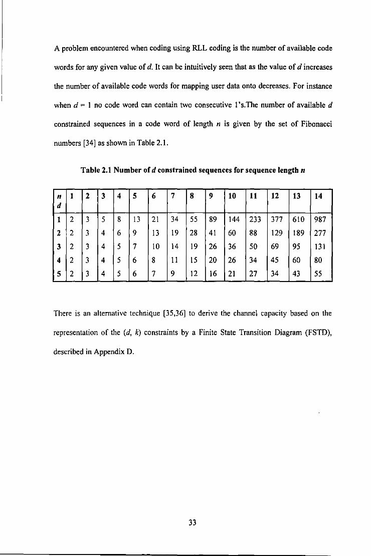
A problem encountered when coding using RLL coding is the number of available code

words for any given value of d. It can be intuitively seen that as the value of d increases

the number of available code words for mapping user data onto decreases. For instance

when d = I no code word can contain two consecutive l's.The number of available d

constrained sequences in a code word of length n is given by the set of Fibonacci

numbers [34] as shown in Table 2.1.

Table 2.1 Number of d constrained sequences for sequence length n

11 1 2 3 4 5 6 7 8 9 10 11 12 13 14 d

1 2 3 5 8 13 21 34 55 89 144 233 377 610 987

2 2 3 4 6 9 13 19 28 41 60 88 129 189 277

3 2 3 4 5 7 10 14 19 26 36 50 69 95 131

4 2 3 4 5 6 8 11 15 20 26 34 45 60 80

5 2 3 4 5 6 7 9 12 16 21 27 34 43 55

There is an alternative technique [35,36] to derive the channel capacity based on the

representation of the (d, k) constraints by a Finite State Transition Diagram (FSTD),

described in Appendix D.

33

2.4.2 Charge Constrained (D.C.-Free) Codes

The importance of d.c.-free codes in magnetic recording has been recognised for a

number of reasons;

a) The use of a d.c.-free code accommodates detection by integration, which for

some noise spectra may be preferable to differentiation.

b) In a.c.-coupled magnetic channels, the transformer or coupling capacitor

prevents d.c. response. Codes which are not d.c.-free may exhibit baseline

wander on readback, making detection more difficult, or in the case of a.c.­

coupled write drivers, may fail to saturate the medium. In particular, d.c.-free

codes are used in nearly all helical scan rotary head recorders employing

rotary transformers.

c) One of the limiting factors in increasing the area! density of magnetic disk

drives is the inability to precisely servo the head positioning mechanism on a

given track. In rotary head tape transports multiple heads with different

azimuth angles often write over neighbouring tracks which slightly overlap,

this deliberate overlap method is called perpetual overwrite. In both these

recorders the problem of crosstalk, that is the side-reading of an adjacent

track, which is primarily a low frequency phenomenon, is diminished by

limiting the low frequency content of the modulation code.

d) Inherently, the read head of many magnetic recording channels is essentially a

flux differentiator and therefore the channel exhibits a spectral null at d.c.

34

D.c.-free codes are not usually employed in current computer peripheral or disk drives.

However, almost all rotary head recorders employ d.c.-free codes to alleviate the

problem of track mis-registration. It is in many ways, a much more difficult engineering

task to "stay on track" with a thin flexible tape wrapped around a helical drum than it is

in other types of magnetic recorders, Therefore a great deal of attention has been paid to

the basic problem of deriving continuous reproduce-head position error signal in rotary

head machines. Rotary head machines also use d.c.-free modulation and channel codes

specifically in order to provide empty or clear parts at the bottom of the spectrum in

which other useful information may be recorded.

D.c.-free code sequences have a balance of charge, that is they exhibit an RDS with an

average of zero. Justesen [37] has shown that to produce a code with a spectral null at

d.c. is equivalent to producing a code with a bounded RDS. To produce a d.c. null with

more rapid roll-off, tighter bounds on the maximum allowable RDS may be introduced

[38], or higher order charge statistics may be constrained.

Norris and Bloomberg [39] have determined the information carrying capacity of (d. k)

codes with bounded RDS, which they refer to as charge constrained run length limited

(CCRLL) codes. Fredrickson [40] describes an alternative method of determining the

capacity of (CCRLL) codes and derives some new charge constrained (d, k) codes.

The disparity of a code word is defined as the difference between the number of O's.and

the number of 1' s in a code word; thus code words 000011, 000 Ill, 001111 have

disparity -2, 0 and 2 respectively.

There are basically three approaches that have been used to create d.c.-balanced codes:

35

a) The most obvious method for the construction of d. c.-free codes is to employ

zero disparity code words. However, this severely limits the code rate, due to

the limited number of zero disparity code words for any given length of code.

b) The next logical step is to extend the above technique to a low disparity code.

Where zero disparity code words are uniquely allocated to the source data

words and pairs of opposite low disparity code words are also used to

represent a single source data word. During recording, the choice of a specific

translation is made in such a way that the accumulated disparity, or RDS is

minimised.

c) Another special case of low-disparity codes, known as polarity bit code, was

devised by Bowers [41] and Carter [42]. In their method a group of (n-1)

source symbols are supplemented by a symbol I. The encoder has the option

to record the resulting n-bit word without modification or to invert all

symbols. Similarly to the previous method, the choice is made to minimise

the accumulated disparity. The last symbol of the code word, called the

polarity bit, is used by the decoder to identify whether the transmitted code

word has been inverted or not.

Recently a new algorithm for generating zero disparity code words has been devised by

Knuth [43]. This method translated the set of m-bit source words to (m+p)-bit balanced

code words. The translation is achieved by selecting a bit position within the m bit code

word that defines two segments each having half of the total disparity. A d.c.-free code

word is generated by the inversion of all bits within one segment. The remaining p bits

of the code word contain a balanced encoding of the bit position that defines the two

segments.

36

2.5 Coding Schemes

A number of attempts have been made to compare different digital recording codes [ 44-

47]. Mackintosh [46) concludes that there is little to chose between all popular codes as

regards maximum packing density, whilst according to Kiwimagi [47] there is no single

best choice for all situations.

It is difficult to place codes in league order when considering them in isolation,

therefore a summary of some of the main characteristics of several of the codes to be

discussed is presented in Table 2.2. Examining this table clearly shows that d.c. free

codes are less efficient than others that do not possess this property.

Consideration must be given to the cost and complexity of implementation and since the

objective is high data rate, error-free recording, compatible equalisation, clock recovery,

error propagation and error detection and correction (EDAC) techniques must be

considered.

Following is a description of some popular coding schemes used for digital recording.

37

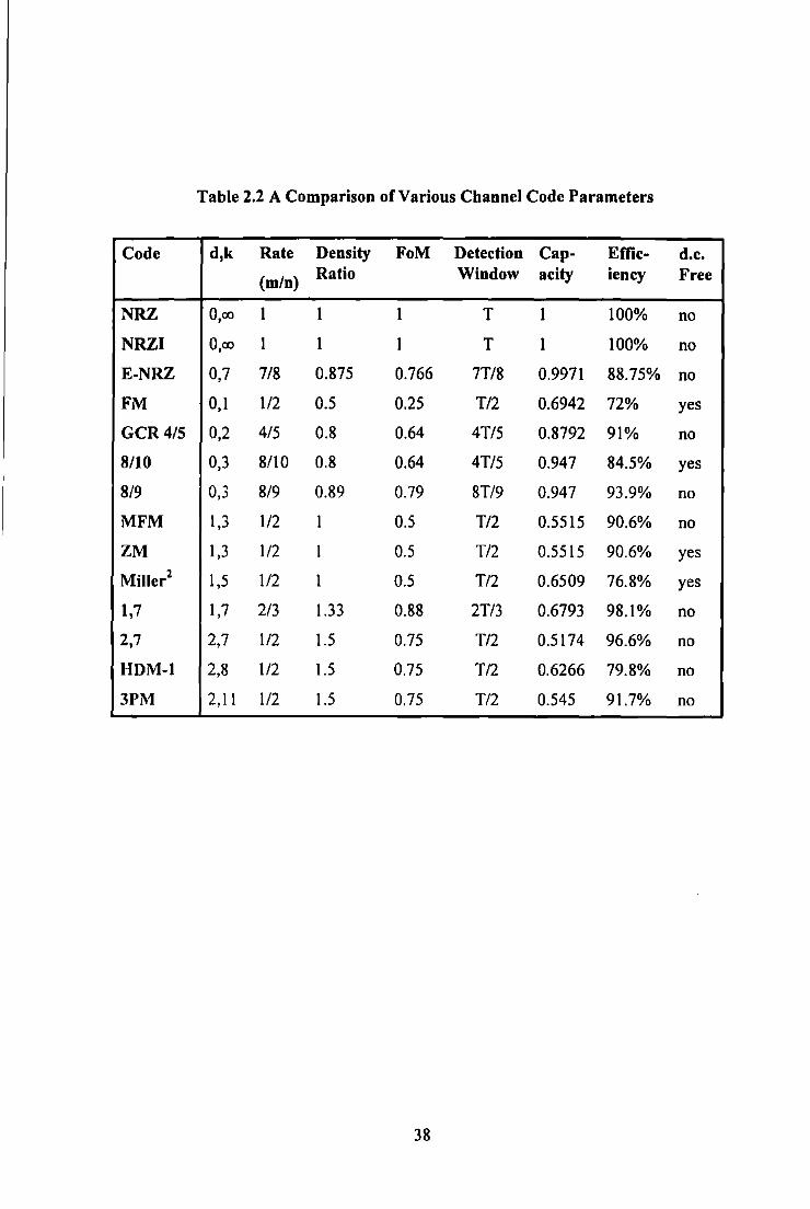
Table 2.2 A Comparison of Various Channel Code Parameters

Code d,k Rate Density FoM Detection Cap- Effic- d.c.

(m/n) Ratio Window a city iency Free

NRZ O,oo I I I T I 100% no

NRZI O,oo I I I T I 100% no

E-NRZ 0,7 7/8 0.875 0.766 7T/8 0.9971 88.75% no

FM 0,1 1/2 0.5 0.25 T/2 0.6942 72% yes

GCR 4/5 0,2 4/5 0.8 0.64 4T/5 0.8792 91% no

8/10 0,3 8/10 0.8 0.64 4T/5 0.947 84.5% yes

8/9 0,3 8/9 0.89 0.79 8T/9 0.947 93.9% no

MFM I ,3 1/2 1 0.5 T/2 0.5515 90.6% no

ZM 1,3 1/2 I 0.5 T/2 0.5515 90.6% yes

Miller 2 I ,5 1/2 1 0.5 T/2 0.6509 76.8% yes

1,7 1,7 2/3 1.33 0.88 2T/3 0.6793 98.1% no

2,7 2,7 1/2 1.5 0.75 T/2 0.5174 96.6% no

HDM-1 2,8 1/2 1.5 0.75 T/2 0.6266 79.8% no

3PM 2,11 112 1.5 0.75 T/2 0.545 91.7% no

38

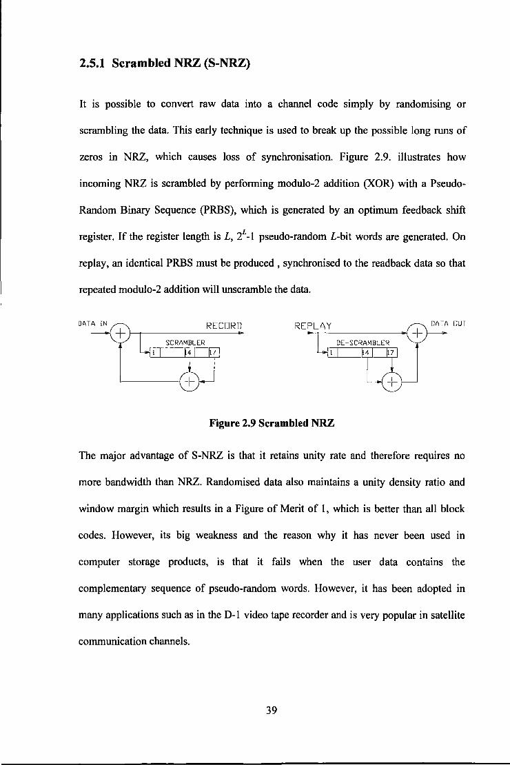
2.5.1 Scrambled NRZ (S-NRZ)

It is possible to convert raw data into a channel code simply by randomising or

scrambling the data. This early technique is used to break up the possible long runs of

zeros in NRZ, which causes loss of synchronisation. Figure 2.9. illustrates how

incoming NRZ is scrambled by performing modulo-2 addition (XOR) with a Pseudo­

Random Binary Sequence (PRBS), which is generated by an optimum feedback shift

register. If the register length is L, 2L -1 pseudo-random L-bit words are generated. On

replay, an identical PRBS must be produced , synchronised to the readback data so that

repeated modulo-2 addition will unscramble the data.

RECORD REPLAY

Figure 2.9 Scrambled NRZ

The major advantage of S-NRZ is that it retains unity rate and therefore requires no

more bandwidth than NRZ. Randomised data also maintains a unity density ratio and

window margin which results in a Figure of Merit of I, which is better than all block

codes. However, its big weakness and the reason why it has never been used in

computer storage products, is that it fails when the user data contains the

complementary sequence of pseudo-random words. However, it has been adopted in

many applications such as in the D-1 video tape recorder and is very popular in satellite

communication channels.

39

2.5.2 Block Codes

Block codes have proved very successful in digital recording systems. Coding is

achieved by partitioning the source data into blocks of length m, which are mapped onto

code words of length n using a conversion table known as a code book.

Manchester Code (Bi-PIIase, PE, FM)

The Manchester group of codes, known also as Bi-phase, Phase Encoding (PE) and

Frequency Doubling, together with Frequency Modulation (FM), were the first self

clocking codes to be developed for direct digital recording. The coding rules for this

family of modulation codes are very simple to implement. For example PE uses a

positive transition at the bit cell centre to represent a logic I and a negative transition

corresponds to a logic 0. Where two or more l's or O's occur in succession, an extra

transition is inserted between them at the bit cell boundary. Similarly for Bi-Phase the

code always changes state at the centre of a bit- cell; the first half of the bit-cell is

encoded as the complement of the data, whilst the second half is the actual data value.

Whereas FM maintains a transition at the bit-cell boundary and employs a transition at

the bit cell centre to represent a logic 1 and no transition to represent a logic 0.

All these codes have run-length constraints of (0, 1) and a code rate of l/2. However,

self clocking is achieved by sacrificing the detection window to half of one bit cell and a

reduction of the density ratio to a l/2. Therefore the FoM for these code is reduced to

0.25. Whilst the low k value facilitates data recovery, the low value of d implies a

potential for excess inter-symbol interference when recording at high data rates.

40

Never-the-less due to the simplicity of these codes and the added advantage that they

possess no d.c. content means they remain widely used today where recording density is

not of prime importance.

Miller Code (MFM, DM))

In Miller code [48], also known as Modified Frequency Modulation (MFM) or Delay

Modulation (OM), the highly redundant clock content of FM was reduced by the use of

a phase-locked loop (PLL) in the receiver that could flywheel over missing clock

transitions. A technique which is implicit in more advanced codes. In Miller code the

presence or absence of a transition at the bit-cell centre, corresponding to a logic I or 0

respectively, was retained but the bit-cell boundary transition is now only required

between successive O's. There are still two channel bits for every data bit, hence the

code rate= 1/2, but adjacent channel bits will never be one, doubling the minimum time

between transitions and giving a OR of I. Miller code, unlike FM, is not d.c.-free and

with run-length constraints of (I ,3) the increased value of k makes data recovery

slightly more difficult.

MFM has been considered a standard code for several years and was adopted for many

hard disks at the time of development and remains in use on double-density floppy

disks. However, it was found that this was not an optimum code and additiomil

improvements have been realised which, make it d.c.-free by bounding the charge

constraint (Zero Modulation [49]), widen the detection window (GRC 4/5 [50]) and

improve the density ratio. These improvements are achieved by an increase in

complexity of encoding/decoding and clock recovery circuits.

41

2.5.3 Variable Length RLL Coding

Attempts to improve the efficiency of fixed length state-dependent codes result in

increased code word length and thus, increased encoder and decoder complexity.

Variable length codes offer the possibility of using short words more frequently than

those of longer length. This is usually profitable in terms of a marked reduction in the

encoder/decoder hardware complexity relative to a fixed length code with the same rate

and run-length constraints.

Manufacturers of magnetic recording systems resist variable rate codes mostly because

they desire a block of data that fits within a fixed size record on the medium and are

concerned that they must accommodate for the worst case data block where the code has

a minimum rate. To overcome this objection the codes are constructed to achieve a

minimum coding rate equal to that of the industry-accepted code rate for a given (d, k)

constraint. If the code designer has additional knowledge about the statistics of non­

random binary digits to be recorded favourable assignment of data sequences to code

sequences can be listed to achieve average rates higher than the (d, k) constraint

capacity.

The structure of variable length codes required to satisfy the run-length constraints is

similar to that for fixed length codes. However, various special features arise from the

presence of words with different lengths. The requirement of synchronous transmission,

coupled with the assumption that each word carries an integer number of information

bits implies that the code word lengths are integer multiples of a basic word length n,

where n is the smallest code word length. Each code word may be of lengthjn,j = l, 2,

..... M. where Mn is the maximum code word length.

42

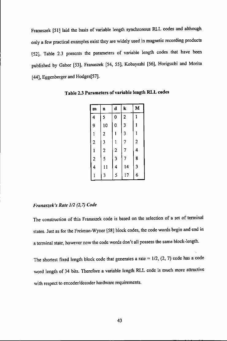
Franaszek [51] laid the basis of variable length synchronous RLL codes and although

only a few practical examples exist they are widely used in magnetic recording products

[52]. Table 2.3 presents the parameters of variable length codes that have been

published by Gabor [53], Franaszek [54, 55], Kobayashi [56], Horiguchi and Morita

[44], Eggenberger and Hodges[57].

Table 2.3 Parameters of variable length RLL codes

m n d k M

4 5 0 2 I

9 10 0 3 I

I 2 I 3 I

2 3 I 7 2

I 2 2 7 4

2 5 3 7 8

4 II 4 14 3

I 3 5 I7 6

Fra11aszek 's Rate 112 (2, 7) Code

The construction of this Franaszek code is based on the selection of a set of terminal

states. Just as for the Freiman-Wyner [58] block codes, the code words begin and end in

a terminal state, however now the code words don't all possess the same block-length.

The shortest fixed length block code that generates a rate = 112, (2, 7) code has a code

word length of 34 bits. Therefore a variable length RLL code is much more attractive

with respect to encoder/decoder hardware requirements.

43

The encoding of incoming data is achieved by dividing the source sequence into two,

three and four bit partitions to match the entries given in the code table, Table 2.4, and

then mapping them into the corresponding channel code word.

For example the data sequence 11010100010 would be split into

11 000 10 0010

which is translated, according to Franaszek's code, into the code word

0100 I 00 I 00 1000 0000 I 000

Table 2.4 g1ves two different coding permutations for a given data sequence as

described by Franaszek [SS] and Eggenberger [57]. There are a total of 24 permutations

of the code word assignments and although at first sight they seem quite arbitrary, they

require careful choice for optimum performance. This is highlighted by the fact that the

Eggenberger code can be decoded using a sliding block decoder with an 8-bit decoder

window length which limits error propagation to a maximum of four bits. Franaszek's

code, however, has the drawback that it requires a 12-bit shift register which increases

error propagation to at most six decoded symbols. This example demonstrates that the

allocation of code words in a variable-length code has a crucial effect on the degree of

error propagation experienced. The optimum code word assignment that minimises error

propagation, as yet, can only be found by trial and error.

44

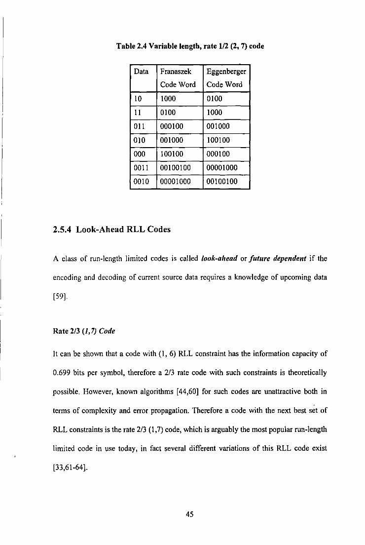
Table 2.4 Variable length, rate 1/2 (2, 7) code

Data Franaszek Eggenberger

Code Word Code Word

10 1000 0100

11 0100 1000

011 000100 001000

010 001000 100100

000 100100 000100

0011 00100100 00001000

0010 00001000 00100100

2.5.4 Look-Ahead RLL Codes

A class of run-length limited codes is called look-ahead or future depe~rdent if the

encoding and decoding of current source data requires a knowledge of upcoming data

[59].

Rate 2/3 (1,7) Code

It can be shown that a code with (1, 6) RLL constraint has the information capacity of

0.699 bits per symbol, therefore a 2/3 rate code with such constraints is theoretically

possible. However, known algorithms [44,60] for such codes are unattractive both in

terms of complexity and error propagation. Therefore a code with the next best set of

RLL constraints is the rate 2/3 (1,7) code, which is arguably the most popular run-length

limited code in use today, in fact several different variations of this RLL code exist

[33,61-64].

45

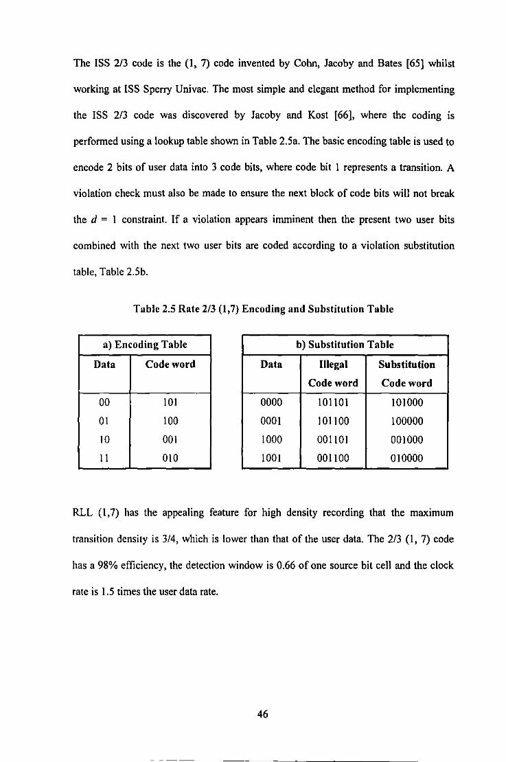
The ISS 2/3 code is the (I, 7) code invented by Cohn, Jacoby and Bates [65] whilst

working at ISS Sperry Univac. The most simple and elegant method for implementing

the ISS 2/3 code was discovered by Jacoby and Kost [66], where the coding is

performed using a lookup table shown in Table 2.5a. The basic encoding table is used to

encode 2 bits of user data into 3 code bits, where code bit I represents a transition. A

violation check must also be made to ensure the next block of code bits will not break

the d = I constraint. If a violation appears imminent then the present two user bits

combined with the next two user bits are coded according to a violation substitution

table, Table 2.5b.

Table 2.5 Rate 2/3 (1,7) Encoding and Substitution Table

a) Encoding Table b) Substitution Table

Data Code word Data Illegal Substitution

Code word Code word

00 I 01 0000 IOIIOI 101000

01 100 0001 lOll 00 100000

10 001 1000 001101 001000

11 010 lOO I OOIIOO 010000

RLL (I, 7) has the appealing feature for high density recording that the maximum

transition density is 3/4, which is lower than that of the user data. The 2/3 {I, 7) code

has a 98% efficiency, the detection window is 0.66 of one source bit cell and the clock

rate is 1.5 times the user data rate.

46

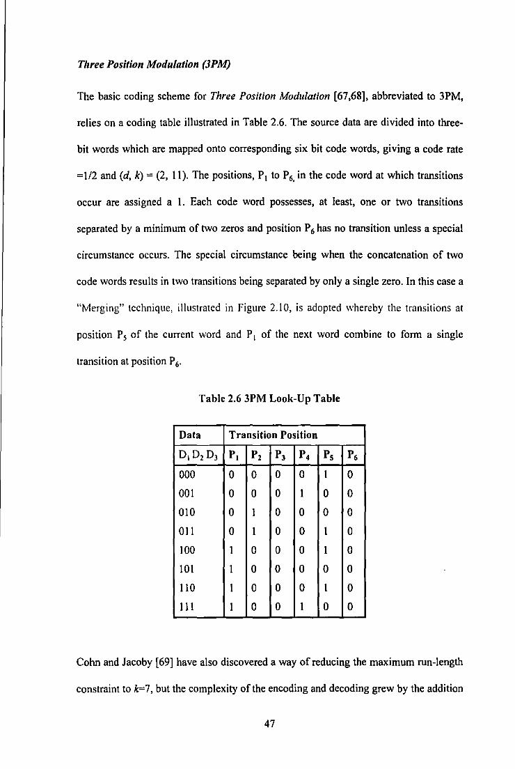
Three Position Modulation (JPM)

The basic coding scheme for Three Position Modulation [67,68], abbreviated to 3PM,

relies on a coding table illustrated in Table 2.6. The source data are divided into three­

bit words which are mapped onto corresponding six bit code words, giving a code rate

=1/2 and (d, k) = {2, 11). The positions, P1 to P6, in the code word at which transitions

occur are assigned a 1. Each code word possesses, at least, one or two transitions

separated by a minimum of two zeros and position P 6 has no transition unless a special

circumstance occurs. The special circumstance being when the concatenation of two

code words results in two transitions being separated by only a single zero. In this case a

"Merging" technique, illustrated in Figure 2.10, is adopted whereby the transitions at

position P5 of the current word and P1 of the next word combine to form a single

transition at position P 6.

Table 2.6 3PM Look-Up Table

Data Transition Position

0 10 2 0 3 PI p2 PJ p4 Ps p6

000 0 0 0 0 l 0

001 0 0 0 1 0 0

010 0 1 0 0 0 0

011 0 1 0 0 1 0

100 1 0 0 0 1 0

101 1 0 0 0 0 0

110 l 0 0 0 l 0

Ill 1 0 0 1 0 0

Cohn and Jacoby [69] have also discovered a way of reducing the maximum run-length

constraint to k=7, but the complexity of the encoding and decoding grew by the addition

47

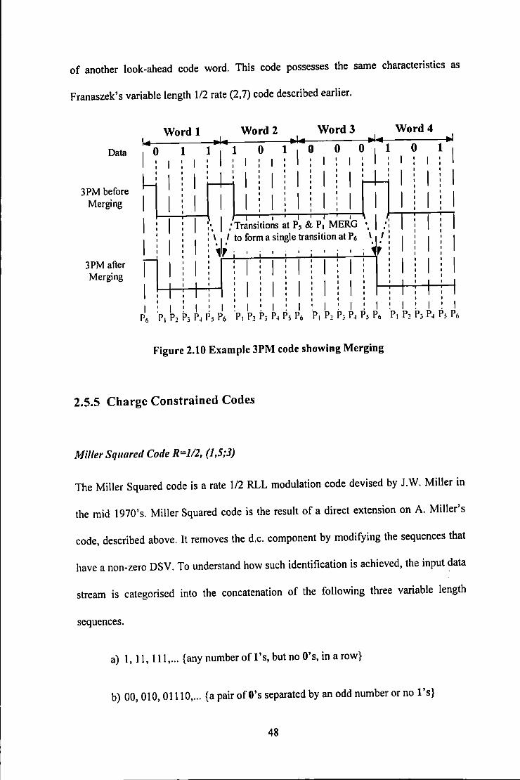
of another look-ahead code word. This code possesses the same characteristics as

Franaszek's variable length 112 rate (2,7) code described earlier.

Data 0

3PM before Merging

3PM after Merging

Word 1

1

Word2 Word3

1 1 0 1 0 0 0 1

I I I

1', ;Transitions at P5 & P1 MERG ·. I .·· \ I·' to form a single transition at P6

,, • I " I I " I " I

\ I ..

I I I I I I I I

Word4 .. 1

0 1

I . I I I . I . I I . I . I I I I I p6 r. p2 p3 p4 P; p6 r. p2 p3 p4 Ps p6 r. p2 p3 p4 P; p6 PI p2 p3 p4 Ps p6

Figure 2.10 Example 3PM code showing Merging

2.5.5 Charge Constrained Codes

Miller Squared Code R=l/2, (1,5;3)

The Miller Squared code is a rate 1/2 RLL modulation code devised by J.W. Miller in

the mid 1970's. Miller Squared code is the result of a direct extension on A. Miller's

code, described above. It removes the d.c. component by modifying the sequences that

have a non-zero DSV. To understand how such identification is achieved, the input data

stream is categorised into the concatenation of the following three variable length

sequences.

a) I, 11, 111, ... {any numberofl's, but no O's, in a row}

b) 00,010, 01110, ... {a pair ofO's separated by an odd number or no l's}

48

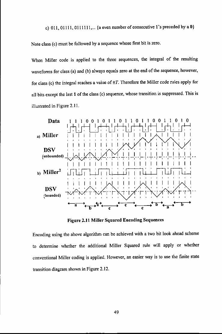
c) 011, 01111, 0111111, ... {a even number of consecutive l's preceded by a 0}

Note class (c) must be followed by a sequence whose first bit is zero.

When Miller code is applied to the three sequences, the integral of the resulting

waveforms for class (a) and (b) always equals zero at the end of the sequence, however,

for class (c) the integral reaches a value of ±T. Therefore the Miller code rules apply for

all bits except the last 1 of the class (c) sequence, whose transition is suppressed. This is

illustrated in Figure 2.11.

Data

a) Miller

DSV (unbounded) I - ------------------------------

1 I I I I I I I I I I I I I I I

I I I

b) Miller2

' '

DSV (bounded)

Figure 2.11 Miller Squared Encoding Sequences

Encoding using the above algorithm can be achieved with a two bit look ahead scheme

to determine whether the additional Miller Squared rule will apply or whether

conventional Miller coding is applied. However, an easier way is to use the finite state

transition diagram shown in Figure 2.12.

49

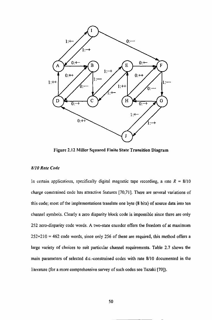
Figure 2.12 Miller Squared Finite State Transition Diagram

8/10 Rate Code

In certain applications, specifically digital magnetic tape recording, a rate R = 8/I 0

charge constrained code has attractive features [70,71). There are several variations of

this code; most of the implementations translate one byte (8 bits) of source data into ten

channel symbols. Clearly a zero disparity block code is impossible since there are only

252 zero-disparity code words. A two-state encoder offers the freedom of at maximum

252+21 0 = 462 code words, since only 256 of these are required, this method offers a

large variety of choices to suit particular channel requirements. Table 2. 7 shows the

main parameters of selected d.c.-constrained codes with rate 8/10 documented in the

literature (for a more comprehensive survey of such codes see Tazaki [70]).

50

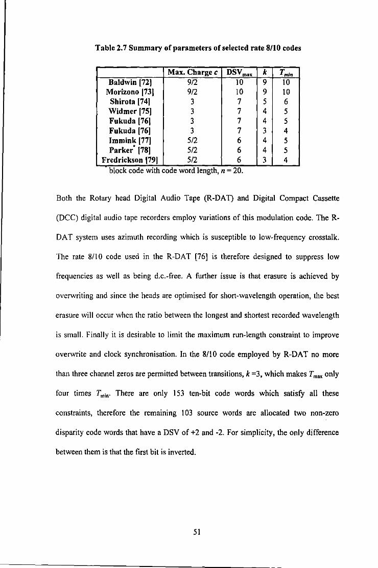
Table 2.7 Summary of parameters of selected rate 8/10 codes

Max. Charge c nsvm .. k Tml,. Baldwin [72) 9/2 10 9 10

Morizono [73) 9/2 10 9 10 Shirota [74) 3 7 5 6 Widmer [75) 3 7 4 5 Fukuda [76) 3 7 4 5 Fukuda [76) 3 7 3 4 Immink [77) 5/2 6 4 5 Parker· [78) 5/2 6 4 5

Fredrickson [79) 5/2 6 3 4 block code With code word length, n = 20.

Both the Rotary head Digital Audio Tape (R-DAT) and Digital Compact Cassette

(DCC) digital audio tape recorders employ variations of this modulation code. The R-

DAT system uses azimuth recording which is susceptible to low-frequency crosstalk.

The rate 8/10 code used in the R-DAT [76] is therefore designed to suppress low

frequencies as well as being d.c.-free. A further issue is that erasure is achieved by

overwriting and since the heads are optimised for short-wavelength operation, the best

erasure will occur when the ratio between the longest and shortest recorded wavelength

is small. Finally it is desirable to limit the maximum run-length constraint to improve

overwrite and clock synchronisation. In the 8/l 0 code employed by R-DAT no more

than three channel zeros are permitted between transitions, k =3, which makes T max only

four times T min· There are only 153 ten-bit code words which satisfy all these

constraints, therefore the remaining I 03 source words are allocated two non-zero

disparity code words that have a DSV of +2 and -2. For simplicity, the only difference

between them is that the first bit is inverted.

51

2.5.6 Convolutional Codes

Convolutional codes have mainly been used as error control codes and not as

modulation codes due to their uncontrollable run-length constraints. As such many

convolutional codes are discovered by computer searches.

Convolutional codes have an additional parameter known as the constraint length, Leo

The constraint length, usually measured in source data bit periods T, describes the

maximum number of prior bits which affect the encoding/decoding of the current data

bit.

This parameter directly relates to the error propagation experienced if a single bit is

detected in error. Therefore if Le is long all errors will be burst errors.

Two codes that can best be described as convolutional [80] due to their complex

encoding algorithms that require numerous exceptions, look-ahead and look back will

be summarised below.

The High Density Modulation (HDM) family of codes [81] has been developed

specifically for Digital Audio Stationary Head (DASH) recorders. HDM-1 code has a

rate 1/2 and (2, 8) run-length constraint which results in a density ratio of 1.5. The

coding algorithm basically treats the source data 01 as a single symbol which has a

transition recorded at the centre of the one. Further transitions are recorded betWeen

lengths of ones and zeros depending on a complex set of conditions requiring a

constraint length of 5.5T. A derivative of this code is HDM-2 which reduces the k

constraint to 7 at the expense of an increased constraint length Le= 7.5T.

52

The 2/4M [82] is another code that is best described as convolutional. This code has a

code rate = 112, run-length constraints of (2, 15) and identical density ratio and window

margin to HDM-1. When encoding a pair of data bits this code requires a look-ahead

and look-back of four source bits. This code has been adopted by the Mitsubishi ProDigi

quarter-inch digital audio stationary head recorder.

2.6 Combined Error Correcting and RLL Coding

In magnetic recording there are many mechanisms available to corrupt data, from the

mechanical problems such as media dropouts and poor head contact, to Gaussian

thermal noise in the replay circuits and heads. Whatever the cause of error the result will

be that the received data will be corrupted with respect to the recorded data. In some

two-way communication channels it is sometimes enough to know that an error has been

detected in which case the receiver can request a retransmission (ARQ). However, this

is quite inappropriate for the digital magnetic recording channel.

A typical encoding configuration for a magnetic recording channel consists of encoding

the bits of information with an error correcting code (ECC) [83] followed by a run

length limited modulation code. The error-correction code is selected according to the

statistics of errors produced by the channel.

One of the problems with this approach is that the demodulator propagates errors whilst

attempting to estimate the correct recorded sequence, therefore a single bit error may

become a burst. Hence the error correction strategy must be able to correct burst errors

even when the noise in the channel is dominated by random errors.

53

Run-length limited codes do have a have a limited capability for error detection during

transmission by identifying violations of the run-length constraints. However, not all

errors result in a run-length violation, therefore several authors have explored the

possibility of producing RLL codes with error correction capabilities.

Ferreira [85] introduced the concept of Hamming-distance preserving RLL codes that

have a Hamming distance between any two encoded sequences greater than or equal to

the Hamming distance of the corresponding input sequences.

An alternative to the traditional concatenation of error correction coding and modulation

coding was proposed by Lee and Wolf [86,87]. The authors use the symbols of a block

modulation code in order to construct a general algorithm for a single error-correcting

RLL code. Based on this technique a number of other authors [88-90] have presented

papers describing combined ECCIRLL trellis codes based on the concatenation of

convolutional codes [91] with run-length limited codes. Immink [92] investigated the

Euclidean distance between ECCIRLL sequences for the noisy digital magnetic

recorder.

Another alternative approach taken by Fredrickson and Wolf [93] concentrated on RLL

codes that can detect transition shifts in a (d, k) constrained sequence. Recently Ytrehus

[94] utilised an exhaustive computer search program to establish the upper and lower

bounds on the size of run-length constraints for error-controlling block codes that have a

minimum specified Hamming distance.

54

2. 7 Multi-Level Signalling

Other communications channels, such as the telephone line, have achieved significant

increases in performance from the use of multi-level, also known as M-ary signalling

techniques [95,96]. M-ary coding schemes for magnetic recording utilise one or more of

the three degrees of freedom that are possible: position, polarity and amplitude. In the

case of binary codes (M =2) the source data are represented using the position of flux

transitions.

Due to the hysteresis of the magnetic recording medium it is not possible to record

directly a multi-level signal. If the recording medium was allowed to take on M-ary

states, the effect of a non-saturating record current would depend not only on the

magnitude of the recording field, but also on the magnitude of the existing

magnetisation state. Since, when recording, it is not possible to know the position on the

hysteresis curve of the existing state of magnetisation for the magnetic medium, the

remanant state of magnetisation after applying a known field would also be unknown.

Mackintosh and Jorgensen [97] have conducted a theoretical investigation into the use

of multi-level coding, the result of which suggests that M-ary signalling techniques are

less efficient than binary codes under most conditions. However, these results were for a

peak detect system and as such did not take into consideration additional benefits that

can be gained from a Viterbi detector.

Over the years several different multi-level techniques have been proposed [98-1 04],

however, these approaches to increase storage density have been resisted in commercial

55

products. The following is a brief review of some multi-level signalling techniques

considered for implementation by the author.

Chi [ 1 OS] proposed a M-ary recording scheme called Controlled Return to AC (CRA)

which utilises a change in the polarity sequence of two recorded dibits or doublets3

. A

high frequency a.c. signal, which in fact erases any previous data, is continuously

recorded, interrupted by short durations that represent the M-ary source symbol. The

advantages of this code are, it is d.c.-free, it has excellent overwrite properties, it offers

SO% improved packing density over Miller code. Chi later revised this code [I 06] by

varying the duration of the doublets to exploit amplitude variation in the readback

signal. This further improved the density ratio to 130% over Miller code. However, the

main disadvantage of this code due to the multi-level signal is that the amplitude of the

readback signal is attenuated by 6dB relative to a conventional recording code.

Jacoby [I 07] describes a multi-level code based on the 3PM coding scheme that doubles

the packing density relative to Miller code. This technique employs the peak shift

between two closely spaced flux transitions to provide the third code state. Therefore

three source words 0, 1 and 2, are represented by the absence and presence of a

transition and a doublet respectively.

A particular ternary modulation technique called controlled polarity modulation [104-

1 09] can be interpreted as a form of write equalisation.[! 10] and is similar to :that

proposed by Veilard [111].

3 Dibit or Doublet is the name given to two closely-spaced transitions.

56

~~

I. I I

'1

0 "

Pilase modulation techniques are. ofte11. rch9~en for ,use in systems: With •non~Ilm!ar

beh~viour, because .of the 'c9J1Stant amplitUde. envelope~ The additionali constraint of

continuous phase lead!) tor signals which .make fuli use "Of· th~ av~jlable c::hannel

.bandwidth. Recently Weathers [Ji12']1 has combined;conyerition:al'RJJ:L codes with;a bias

signal rto ,achieve weater packing, ;densities, This Work "W!lS; furtheredi [113J]i using a

conv:entionali modem to ·record' data on;a rotary head tape with sl)rprisingly good results,

lfohe mtidl':iil' Iinearises the rchanneil,l)y modul~ting data' on. to 'a carrier signaJ and uses

.quadnjtllt'e a111plitude -modulation (QAM). ii:l' cin1j\.Jnctiopr with trellis ;coded modulation

r(TCM): to obtain· increased performance, A -similar tec]mique has also I been proposed by

KObaYaslli' et al. [1:114'] to; increase· the. recorciihg efficiency rof a video .cassette. recorder.

57

2.8 Summary

Modulation codes have been used with great success in magnetic and optical storage to

increase linear density and improve performance. These codes represent the result of a

steady evolution of channel code design for a particular detection technique, namely

peak detection, employed in most storage systems. It is difficult to quantify the increase

in storage capacity that RLL coding affords since it varies with the detection circuitry

used. By way of an example Immink calculates that for a compact disc system the RLL

scheme increases capacity by approximately 25% over that of the uncoded medium.

Several different run-length limited and charge constrained modulation coding

techniques have been described that are or have been used in various magnetic recording

channels. The choice of the optimum modulation code for any particular device involves

trade-offs between the various properties of the modulation code and the characteristics

of the channel in which it is to be applied. A prime example is the choice of modulation

coding for magnetic hard disk drives.

Research on RLL coding schemes continues, however most current work aims at

combining error correction codes with RLL codes. These integrated codes offer

increased efficiency and reliability over individual error correction and modulation

codes applied consecutively to the source data. However, no such code has yet been

included in a commercial device. The author believes that if peak detection is to

maintain a position in commercial storage devices combined ECCIRLL codes will have

to be employed.

58

2.9 References

I. Shannon, C.E., "A Mathematical Theory of Communications", Bell Syst. Tech.

Journal, Vol.27, No.3, pp.379-423:623-656, July 1948.

2. Mallinson, J.C., "The Foundations of Magnetic Recording", Academic Press, Inc

(London) Ltd., 1987.

3. Mallinson, J.C., "Theory of Linear Superposition in Tape Recording", IEEE

Trans. Magn., Vol.S, No.4, pp.886-90, December 1969.

4. Melbye, H.E., & Chi, C.S., "Non-linearities in High Density Digital Recording",

IEEE Trans. Magn., Vol.14, No.S, pp. 746-48, 1978.

5. Koren, N., "A Simplified Model of Non-linear Bit Shift in Magnetic Recording",

Intermag'91, France. 1991.

6. Melas, G.M., et al. "Non-Linear Superposition in Saturation Recording of Disk

Media", IEEE Trans. Magn., Vo1.23, No.S, pp.2019,21, 1987.

7. Rijckaert, M.A., et a!, "Magnetic Head Mounting Mechanism for Automatic

Azimuth Control", U.S. Patent 4,451,862., 29 May 1984.

8. Rijckaert, M.A., et a!, "Magnetic Tape Recording and/or Reproducing Appartatus

with Automatic Head Positioning", U.S. Patent 4,392, 163., 5 July 1984.

9. Niet, E.D., "Azimuth Correction of Head Gaps", U.S. Patent 4,317,144., 23

February 1982.

10. Lemke, J.U., "Magnetic Playback Apparatus Having Immunity to Skew", U.S.

Patent 4,330,807., 18 May 1982.

59

11. Donnelly, T., Mapps, D.J., & Wilson, R. "Real-Time Microprocessor Monitoring

of Skew Angle in a Compact Cassette Multitrack Magnetic Tape System",

J.IERE. Vol.56, No.2, pp.49-52, February 1986.

12. Parkinson, J., "Data Recording and its Problems", Radio Commun., Vol.60, No. I,

pp.32-35, January 1984.

13. Perry, M.A., et al., "The Importance of Dropout Measurement in Ensuring Good

Short Wavelength Recording on Magnetic Tape", 4th Int. Conf. on Video, Audio

& Data Recording, pp.23-41, 20-23 April 1982.

14. Meeks, L.A., "Dropout Characteristics of Instrument Tape and Approach to Error

Correction.", Electronic Engineering, pp.ll7-128 March 1982.

15. Jacoby, G.V., "High Density Recording with Write Current Shaping", IEEE

Trans. Magn., Vol.l5, pp.ll24-, 1979.

16. Thomley, R.F.M., "Compensation ofPeak-Shift with Write Timing", IEEE Trans.

Magn., Vol.l7, No.6, pp.3332-34, November 1981.

17. Schneider, R.C., "Write Equalization in High-Linear-Density Magnetic

Recording", IBM J. Res. Develop., Vol.29, No.6, pp.563-68, November 1985.

18. Veilard, D.H., "Compact Spectrum Recording, A New Binary Process

Maximizing the use of a Recording Channel", IEEE Trans. Magn., Vol.20, No.5,

pp.891-93, September 1984.

19. Tomlinson, M., "New Automatic Equalizer Employing Modulo Arithmetic",

Electronic Lett., Vol.7, No.5/6, pp.l38-39, 25 March 1971.

20. Harashima, H., & Miyakawa, H., "Matched Transmission Technique for Channels

with Inter-Symbol Interference", IEEE Trans Comms., Vol.20, pp.774-80, August

1972.

60

21. Fomey, Jr., G.D., & Eyuboglu, M.V., "Comined Equalization and Coding Using

Precoding", IEEE Comms. Magazine, pp.25-34, December 1991.

22. Sierra, H.M., "Increased Magnetic Recording Readback Resolution", IBM Tech.

Disclosure Bulletin, Vo1.7, No. I, pp.22-33, 1963.

23. Jacoby, G.V., "Signal Equalization in Digital Magnetic Recording", IEEE Trans.

Magn., Vol.4, pp.302-05, September 1968.

24. Schneider, R.C., "An Improved Pulse-Slimming Method for Magnetic

Recording", IEEE Trans. Magn., Vol.l1, No.5, pp.l240-41, September 1975.

25. Kameyama, T., Takanami, S., & Arai, R., "Improvement of Recording Density by

means of Cosine Equalization", IEEE Trans. Magn., Vol.12, No.6, pp.746-48,

November 1976.

26. Mackintosh, N.D., "A Superposition-Based Analysis of Pulse Slimming

Techniques for Digital Recording", The Radio & Electronic Eng., Vol.50, No.6,

pp.307-14, June 1980.

27. Barbosa, L.C., "Minimum Noise Pulse Slimmer", IEEE Trans. Magn., Vol.MAG-

17, No.6, pp.3340-42, November 1981.

28. Proakis, J.G., "An Improved Pulse Slimming Method for Magnetic Recording",

IEEE Trans. Magn., Vol. II, No.5, pp.l240-41, September 1985.

29. Siege!, P.H., "Application of a Peak Detection Channel", IEEE Trans. Magn.,

Vo1.16, No.6, pp.l250-52, November 1982.

30. Immink, K.A.S., "Coding Techniques for Digital Recorders", Prentice Hall, 1991.

31. Tang, D., & Bahl, L., "Block Codes for a Class of Constrained Noiseless

Channels", Information and Control, Vo1.17, pp.436-61, 1970.

61

32. lmmink, K.A.S., "Some Statistical Properties of Maxentropic Run Length Limited

Sequences", Philips J. Res., Vol.38, No.3, pp.138-49, 1983.

33. Franaszek, P.A., "Efficient Code for Digital Magnetic Recording", IBM Tech.

Disclosure Bulletin, Vol.23, No.9, pp.4375-78, February 1981.

34. Kautz, W.H., "Fibonacci Codes for Synchronisation Control", IEEE Trans. lnf.

Theory, Vol.l1, pp.284-92, April 1965.

35. Franaszek, P.A., "Sequence State Coding for Digital Transmission", Bell Sys.

Tech. J., Vol.47, pp.143-57, December 1968.

36. Franaszek, P.A., "Sequence-State Methods for Run-length-limited Coding", IBM

J. Res. Develop., Vol.l4, pp.376-83, July 1970.

37. Justesen, J., "Information Rates and Power Spectra of Digital Codes", IEEE Tran.

Inf. Theory, Vol.28, No.3, pp.457-, March 1982.

38. Immink, K.A.S., "Spectrum Shaping with Binary DC2 Constrained Codes",

Philips J. Res., Vol.40, No.l, pp.40-53, 1985.

39. Norris, K, & Bloomberg, D.S., "Channel Capacity of Charge Constrained Run

Length Limited Codes", IEEE Trans. Magn., Vol.17, No.6, pp.3452-55,

November 1981.

40. Fredrickson, L.J., "On the Shannon Capacity of DC- and Nyquist-Free Codes",

IEEE Trans. Inf. Theory, Vol.37, No.3, pp.918-23, May 1991.

41. Bowers, F.K., U.S. Patent No. 2,957,947., 1960.

42. Carter, R.O., "Low Disparity Binary Coding System", Electron. Lett., Vol.l,

pp.65-68, 1965.

43. Knuth, D.E., "Efficient Balanced Codes", IEEE Trans. Inf. Theory, Vol.32, No. I,

pp.51-53, January 1986.

62

44. Horiguchi, T., & Morita, K., "An Optimization of Modulation Codes in Digital

Recording", IEEE Trans. Magn., Vo1.12, No.6, pp.740-42, November 1976.

45. Mallinson, J.C., & Miller, J.W., "Optimal Codes for Digital Magnetic Recording",

The Radio & Electronic Eng., Vol.47, No.4, pp.l72-76, April1977.

46. Mackintosh, N.D., "The Choice of a Recording Code", IERE Conf. on Video &

Data Recording, pp. 77-119, 24-27 July 1979.

47. Kiwimagi, R.G., Judson, A.M., & Ottesen, H.H., "Channel Coding for Digital

Recording", IEEE Trans. Magn., Vol.IO, No.3, pp.515-18, September 1974.

48. Miller, A., "Transmission System", US Patent 3,108,261., October 1963.

49. Patel, A.M., "Zero Modulation Encoding in Magnetic Recording", IBM J. Res.

Develop., Vol.l9, pp.366-78, July 1975.

50. Tamura, T., Tsutumi, M., Aoi, H., Matsuishi, H., Nakagoshi, K., Kawano, S., &

Makita, M., "A Coding Method in Digital Magnetic Recording", IEEE Trans.

Magn., Vol.8, pp.612-14, September 1972.

51. Franaszek, P.A., "On Synchronous Variable Length Coding for Discrete Noiseless

Channels", Information & Control, Vo1.15, pp.155-64, 1969.

52. Howell, T.D., "Analysis of Correctable Errors in IBM 3380 Disk File", IBM J.

Res. & Develop., Vol.28, No. 2, pp.206-211, March 1984.

53. Gabor, A., "Adaptive Coding for Self Clocking Recording", IEEE Trans. Elec.

Computers, pp.866-68, December 1967.

54. Franaszek, P.A., "Coding for Constrained Channels: A Comparison of Two

Approaches", IBM J. Res. Develop., Vol.33, No.6, pp.602-08, November 1989.

SS. Franaszek, P.A., "Run-Length-Limited Variable Length Coding with Error

Propagation Limitation", U.S. Patent 3,689,899., 5 September 1972.

63

56. Kobayashi, H., "A survey of Coding Schemes for Transmission or Recording of

Digital Data", IEEE Trans on Comm., Vol.COM-19, No.6, pp.1087-1100,

December 1971.

57. Eggenberger, J.S., & Hodges, P., "Sequential Encoding and Decoding of Variable

Word Length, Fixed Rate Data Codes", U.S. Patent 4,115, 768., 19 September

1978.

58. Freiman, C.V., & Wyner, A.D., "Optimum Block Codes for Noiseless Input

Restricted Channels", Information and Control, Vo1.7, pp.398-415, 1964.

59. Lempel, A., & Cohn, M., "Look Ahead Coding for Input Restricted Channels",

IEEE Trans. Inf. Theory, Vo1.28, No.6, pp.933-37, November 1982.

60. Adler, R.L., Brayton, R.K., Hassner, M., & Kitchens, B.P., "A Rate 2/3 (1,6) RLL

Code", IBM Tech. Disclosure Bulletin, Vol.27, No.B, pp.4727-4729, January

1985.

61. Jacoby, G.V., "A New Look Ahead Code for Increased Data Density", IEEE

Trans. Magn., Vo1.13, No.5, pp.1202-04, September 1977.

62. Weathers, A.D., & Wolf, J.K., "A New 2/3 Sliding Block Code for the (1,7)

Runlength Constraint with the Minimum Number of Encoder States", IEEE Trans.

Inf. Theory, Vol.37, No.3, pp.908-913, May 1991.

63. Adler, R., Hassner, M., Kitchens, & Moussouris, P., "Method and Apparatus for

Generating Sliding Block Code for a (1,7) Channel with Rate 2/3", US Patent

4,413,251., 1 November 1983.

64. Baldwin, J.L.E., "A Variation of the 2/3 Channel Code using Block Coding",

IERE 6th lnt. Conf. Video, Audio & Data Rec., pp.157-63, 18-21 March 1986.

64

65. Cohn, M., Jacoby, G.V., & Bates, A., "Data Encoding Method and System

Employing Two Thirds Code Rate with Full Word Look Ahead", US Patent

4,337,458. 29th June 1982.

66. Jacoby, G.V., & Kost, R., "Binary Two-Thirds Rate Code with Full Word Look­

Ahead", IEEE Trans. Magn., Vol.20, No.5, pp.709-14, September 1984.

67. Jacoby, G.V., "A New Look Ahead Code for Increased Data Density", IEEE

Trans. Magn., Vol.l3, No.5, pp.l202-04, September 1977.

68. Nottley, G.C., "3 Position Modulation (3PM) ; A Technical Appraisal", Fourth

Int. Conf. on Video & Data Rec., (20-23 April, Southhampton, U.K.) 1982.

69. Cohn, M., & Jacoby, G.V., "Run-Length Reduction of3PM Code via Look-Ahead

Technique", IEEE Trans. Magn., Vo1.18, No.6, pp.l253-55, November 1982.

70. Tazaki, S., Takeda, F., Osawa, H., & Yamada, Y., "Performance Comparisons of

8-10 Conversion Code", IERE Int. Con f. Video & Data Rec., (Southampton),

pp.79-84, \984.

71. Furukawa, T., Ozaki, M., & Tanaka, K., "On a DC Free Block Modulation Code",

IEEE Trans. Magn., Vo1.20, No.5, pp.878-883, \984.

72. Baldwin, J.L.E., "Digital Television Recording with Low Tape Consumption",

IBC'78, pp.\33-36, 1978.

73. Morizono, M., Yoshida, H., & Hashimoto, Y., "Digital Video Recording- Some

Experiments and Future Considerations", SMPTE Journal, Vol.89, pp.658-62,

1980.

74. Shirota, N., "Method & Apparatus for Reducing DC Component in Digital

Information Signal", US Patent 4,387,364., 7 June 1983.

65

75. Widmer, A.X., & Franaszek, P.A., "A DC Balanced, Partitioned Block 8B/10B

Transmission Code", IBM J. Res. Develop., Vo1.27, No.5, pp.440-51, September

1983.

76. Fukuda, S., Kojima, Y., Shimpuku, Y., & Odaka, K., "8/10 Modulation Codes for

Digital Magnetic Recording", IEEE Trans. Magn., Vol.22, No.S, pp.l194-96,

September 1985.

77. Immink, K.A.S., "Construction of Binary DC-Constrained Codes", Philips J. Res.,

Vol.40, No.1, pp.22-39, 1985.

78. Parker, M.A., & Bellis, F.A., "Signal Processing for an Experimental 216 Mbit/s

Ditial Video Tape Recorder", Proc. 4th Int. Conf. on Video & Data Recording,

(Southampton), pp.207-15, 1982.

79. Fredrickson, L.J., "A (D,K,C)=(0,3,5/2) Rate 8/10 Modualtion Code", IEEE

Trans. Magn., Vo\.26, No.5, pp.2318-20, September 1990.

80. Watkinson, J.R., "The Art Of Digital Audio", Focal Press, 1988.

81. Doi, T.T., "Channel Coding for Digital Audio Recordings", J. Audio Eng. Soc.,

Vo1.31, No.4, pp.224-38, Aprill983.

82. Anon., "PD format for stationary head type 2-channel digital audio recorder",

Mitsubishi, January 1986.

83. Lin, S., & Costello, D.J., "Error Control Coding: Fundamentals and

Applications", Prentice Hall, 1983.

84. Blaum, M., "Combining ECC with Modulation: Performance Comparisons",

IEEE Globecom '90 (San Deigo, CA.,), 901.3, Vol.3, pp.1778-81, December

1990.

66

85. Ferreira, H.C., et al., "Binary Rate 4/8 Runlength Constrained Error Correcting

Magnetic Recording Modulation Code", IEEE Trans. Magn., Vol.22, No.S,

pp.1197-99, September 1986.

86. Lee, P., & Wolf, J.K., "Combined Error Correction/Modulation Codes", IEEE

Trans Magn., Vol.23, No.S, pp.3681-83, November 1988.

87. Lee, P., & Wolf, J.K., "A General Error Correcting Code Construction for Run­

Length Limited Binary Channels", IEEE Trans. Inf. Theory, Vol.35, No.6,

pp.1330-35, November 1989.

88. Lin, Y., & Wolf, J.K., "Combined ECCIRLL Codes", IEEE Trans Magn., Vol.24,

No.6, pp.2527-29, November 1988.

89. French, C.A., & Lin, Y., "Performance Comparison of Combined ECCIRLL

Code", IEEE Int. Conf. Comms. (ICC '90), Vol.4, Session 347.3.1-3.6, pp.l717-

22, Atlanta 1990.

90. Ferreira, H.C., "The Synthesis of Magnetic Recording Trellis Codes with Good

Hamming Distance", IEEE Trans. Magn., Vol.21, No.S, pp.l356-58, September

1985.

91. Forney, Jr., G.D., "Convolutional Codes I: Algebraic Structure", IEEE Trans. Inf.

Theory, Vo1.16, No.6, pp.720-38, November 1970.

92. Immink, K.A.S., "Coding Techniques for the Noisy Magnetic Recording Channel:

A State-of-the-Art Report", IEEE Trans. Comrns., Vol.37, pp.413-419, May 1989.

93. Fredrickson, L.J., & Wolf, J.K., "Error Detecting Multiple Block (d,k) Codes",

IEEE Trans. Magn., Vol.25, pp.4096-98, September 1989.

94. Ytrehus, 0., "Upper Bounds on Error Correcting Runlength Limited Block

Codes", IEEE Trans. Inf. Theory, Vol.37, No.3, pp.941-45, May 1991.

67

95. Sipress, J.M., "A New Class of Selected Ternary Pulse Transmission Plans for

Digital Transmission Lines", IEEE Trans. Comms. Tech., Vol.l3, No.3, pp.366-

72, September 1965.

96. Van Gerwen, P.J., "Efficient Use of Pseudo-Ternary Codes for Data

Transmission", IEEE Trans. Commun. Tech., pp.658-60, August 1967.

97. Mackintosh, N.D., & Jorgensen, F., "An Analysis of Multi- Level Encoding",

IEEE Trans. Magn., Vol.l7, No.6, pp.3329- 31, November 1981.

98. Crossier, A., "Introduction to Pseudo-Ternary Transmission Codes", IBM J. Res.

Develop., Vol.l4, No.4, pp.354-67, July 1970.

99. Tazaki, S., & Yamada, "Decisive Factors to Perforn1ance of Ternary Recording

Code", IEEE Trans. Magn., Vol.27, No.6, pp.4918-20, November 1991.

100. Tazaki, S., Kaji, S., Yamada, Y., & Osawa, H., "Channel Capacity of DC-Free

Ternary Recording Codes", IERE 8th Int. Conf. on Video, Audio & Data

Processing, pp.151-53, 24-26 Aprill990.

101. Vinding, J.P., "Detector Circuits for Ternary Coded Magnetic Recording", IEEE

Trans. Magn., Vol.20, No.5, pp.894-96, September 1984.

102. Vinding, J.P., "Implementation of a Ternary Coder/Decoder", IEEE Trans. Magn.,

Vol.l8, No.6, pp.l256-58, November 1982.

103. Krueger, D., & Cruz, J.R., "Combined Equalization and Ternary Coding for the

Magnetic Recording Channel", IEEE Trans. Magn., Vol.29, No.6, pp.4050-52,

November 1993.

I 04. French, C.A., Dixon, G.S., & Wolf, J.K., "Results Involving (D,K) Constrained

M-ary Codes", IEEE Trans. Magn., Vol.23, No.5, pp.3678-80, September 1987.

68

105. Chi, C.S., & Frey, K.A., "CRA for Ternary Digital Recording", IEEE Trans.

Magn., Vol.l8, No.6, pp.l259-6l, November 1982.

l 06. Chi, C.S., "Triplex Code for Quaternary High Density Recording", IEEE Trans.

Magn., Vol.20, No.5, pp.888-90, September 1984.

107. Jacoby, G. V., "Ternary 3PM Magnetic Recording Code and System", IEEE Trans.

Magn., Vol.l7, No.6, pp.3326-28, November 1981.

108. French, C.A., Weathers, A.D., & Wolf, J.K., "A Generalized Scheme for

Generating and Detecting Recording Channel Output Waveforms with Controlled

Pulse Polarity", IEEE Trans. Magn., Vol.24, No.6, pp.2530-32, November 1988.

I 09. Weathers, A. D., French, C.A., & Wolf, J.K., "Results on 'Controlled Polarity'

Modulation and Coding", IEEE Trans. Magn., Vol.25, No.5, pp.4090-92,

September 1989.

ll 0. Schneider, R.C., "Write Equalization in High-Linear-Density Magnetic

Recording", IBM J. Res. Develop., Vol.29, N0.6, pp.563-68, November 1985.

Ill. Veilard, D.H., "Compact Spectrum Recording, A New Binary Process

Maximizing the use of a Recording Channel", IEEE Trans. Magn., Vol.20, No.5,

pp.891-93, September 1984.

112. Weathers, A.D., & Wolf, J.K., "Biased Run Length Limited Modulation", IEEE

Trans. Magn., Vol.27, No.6, pp.4807-09, November 1991.

113. Weathers, Anthony D., "Modulation Techniques for Digital Magnetic Recording",

PhD Thesis, 1990

114. Kobayashi, M., Ohta, H., Nakatsu, E., Shimazaki, H., & Nagaota, Y., "Quadrature

Amplitude Modulation Recording for Digital VCRs", IERE 8th Int. Conf. Video

Audio & Data Rec., pp.ll6-19, 1990.

69

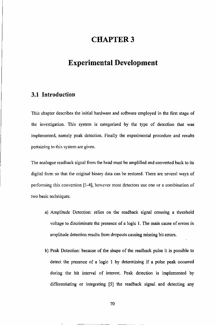
CHAPTER3

Experimental Development

3.1 Introduction

This chapter describes the initial hardware and software employed in the first stage of

the investigation. This system is categorised by the type of detection that was

implemented, namely peak detection. Finally the experimental procedure and results

pertaining to this system are given.

The analogue readback signal from the head must be amplified and converted back to its

digital form so that the original binary data can be restored. There are several ways of

perfom1ing this conversion [1-4], however most detectors use one or a combination of

two basic techniques.

a) Amplitude Detection: relies on the readback signal crossing a threshold

voltage to discriminate the presence of a logic 1. The main cause of errors in

amplitude detection results from dropouts causing missing bit errors.

b) Peak Detection: because of the shape of the readback pulse it is possible to

detect the presence of a logic 1 by determining if a pulse peak occurred

during the bit interval of interest. Peak detection is implemented by

differentiating or integrating [5] the readback signal and detecting any

70

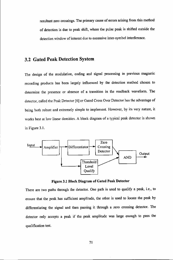
resultant zero crossings. The primary cause of errors arising from this method

of detection is due to peak shift, where the pulse peak is shifted outside the

detection window of interest due to excessive inter-symbol interference.

3.2 Gated Peak Detection System

The design of the modulation, coding and signal processing m previous magnetic

recording products has been largely influenced by the detection method chosen to

determine the presence or absence of a transition in the readback waveform. The

detector, called the Peak Detector [6] or Gated Cross Over Detector has the advantage of

being both robust and extremely simple to implement. However, by its very nature, it

works best at low linear densities. A block diagram of a typical peak detector is shown

in Figure 3.1.

Zero In lpUt

Amplifier ~ Differentiator - Crossing

1\ Detector Outp ut

Threshold~ AND

Level Qualify

Figure 3.1 Block Diagram of Gated Peak Detector

There are two paths through the detector. One path is used to qualify a peak, i.e_., to

ensure that the peak has sufficient amplitude, the other is used to locate the peak by

differentiating the signal and then passing it through a zero crossing detector. The

detector only accepts a peak if the peak amplitude was large enough to pass the

qualification test.

71

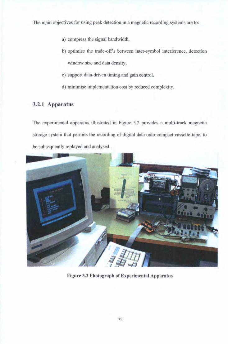
The llij:lm objectives for using peak detection in a magnetic recording systems are to:

a) compress the signal bandwidth,

b) optimise the trade-off's between inter-symbol interference, detection

window size and data density,

c) support data-driven timing and gain control,

d) minimise implementation cost by reduced complexity.

3.2.1 Apparatus

The experimental apparatus illustrated in Figure 3.2 provides a multi-track magnetic

storage system that permits the recording of digital data onto compact cassette tape, to

be subsequently replayed and analysed.

Figure 3.2 Photograph of Experimental Apparatus

72

The basic items of equipment used in this investigation consist of a compact-cassette

tape transport interfaced to a microprocessor control board to form a simple direct

digital recording system. The interface elements comprise read/write amplifiers plus

tape transport circuitry.

A circuit was designed and constructed to contain the digital electronics which include:

the microprocessor; the program memory stored in Erasable Programmable Read Only

Memory (EPROM); a 16 bit programmable up/down counter; an interface for a IBM

compatible host computer; an interface for the read/write electrorucs; and the control

logic The basic elements of the microprocessor control board are shown in Figure 3.3.

The read/write electronics are housed on a small wire-wrap board which could be

mounted near the head to minimise noise.

llNT .------------

ADDRESS

DECODE

ADD RESS BUS

EPROM

8K X 16

CONTROL BUS

PARALLEL INTERFACE

CONTROL

PORT

16BIT

COUNTER/

READ/WRITE

PORT

CIISS<Ite Recorder

OCJO

READ AMPLIFIER + WRITE AMPLIFI ER

PEAK DETECTOR

Figure 3.3 Basic Elements of Recording System 1

73

Compact Cassette

The tape transport comprised a commercial 4-track, audio-frequency, inductive head in

conjunction with a standard solenoid controlled compact cassette mechanism. The head,

tapes and mechanism were employed to provide a cost effective means of achieving a

multi-track system.

The tape speed for a compact cassette tape transport is 4.15 cm/s with a tolerance

ranging up to ±2%, depending on the quality of the device. The low-cost mechanism

employed had poorly controlled motor velocity, eccentricity of the capstan and capstan

shaft, as well as inconsistent friction between bearings, drive belts, and between the tape

and its pressure pad and tape guides. However for the purpose of this investigation these

abnormalities proved ideal to test the ability of intelligent software techniques.

The compact cassette tape transport mechanism employed was solenoid controlled by

the microprocessor via a custom built interface containing solenoid driver amplifiers.

All experimental work was carried out using the 4-track head, however it was envisaged

that heads with greater track densities would be available for experiment during the

investigation. Therefore all the electronics were designed to allow additional channels to

be included as they became available.

TMS 32010 Digital Sig11al Processor

The Texas Instruments TMS320l 0 is a first generation digital signal processor [7]. The

structure of the TMS320l 0 takes advantage of the Harvard Architecture, in which

program and data memory area are separate to permit a full overlap of fetch and

execution of instructions. Texas Instruments further modified this architecture to allow

74

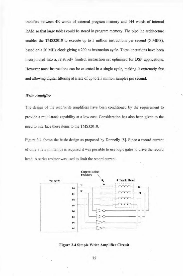
transfers between 4K words of external program memory and 144 words of internal

RAM so that large tables could be stored in program memory. The pipeline architecture

enables the TMS320 10 to execute up to 5 million instructions per second (5 MIPS),

based on a 20 MHz clock giving a 200 ns instruction cycle. These operations have been

incorporated into a, relatively limited, instruction set optimised for DSP applications.

However most instructions can be executed in a single cycle, making it extremely fast

and allowing digital filtering at a rate of up to 2.5 million samples per second.

Write Amplifier

The design of the read/write amplifiers have been conditioned by the requirement to

provide a multi-track capability at a low cost. Consideration has also been given to the

need to interface these items to the TMS320 10.

Figure 3.4 shows the basic design as proposed by Donnelly [8). Since a record current

of only a few milliamps is required it was possible to use logic gates to drive the record

head. A series resistor was used to limit the record current.

Current select

74LS373

resistors ~

4 Track Head

'1' Rt

DO '0'

D1

D2

DJ

D4

DS

D6

D7

Figure 3.4 Simple Write Amplifier Circuit

75

Read Amplifier including Gated Peak Detector

The basic read amplifier design, as described in [9], is illustrated in Figure 3.5. The

signals at each stage of the amplifier are shown graphically in Figure 3.6.

The reproduced signal is sliced to convert the peaks into pulses. These are gated with a

coincident pulse derived from the differential of the signal. First a pre-amplifier

increases the signal level and converts the high output impedance of the read head to a

low impedance. The signal is then passed through a low pass filter to remove any high

frequency noise. A further stage of amplification follows after which the signal path

divides. Along the first path the signal is sliced at a positive and negative level and the

two outputs are applied to two NAND gates. Along the second path the signal is

differentiated to shift it by 90 degrees; this converts the peaks of the signal to zero

crossing points. These points are detected by a comparator that converts them to signal

transitions. The signal to noise ratio at the comparator input is degraded by 6 dB due to

the differentiator. To prevent the noise signal generating a false output, threshold

hysteresis is employed. The edges are converted to pulses which are applied to the

second input of the NAND gates. The output of the NAND gates are used to control a

set/reset flip-flop that delivers a pulse train corresponding to the direction of the second

recorded flux.

The double detection action of the circuit reduces the possibility of false triggering of

the flip-flop due to points of inflection of the differentiated signal. The slice levels are

adjusted to allow for variations in signal amplitude with record frequency.

76

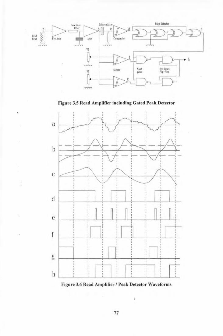
Read Head

"'''e

~--- I h

I rr-h-.

-1·e

1-Figure 3.5 Read Amplifier including Gated Peak Detector

a

b

c

d

c

f

g

h Figure 3.6 Read Amplifier I Peak Detector Waveforms

77

Host Computer

An IBM compatible personal computer (PC) was interfaced to this system to provide a

means to store and analyse the results. The host computer was also used to develop and

debug all software written in assembly language for the TMS 32010 microprocessor and

Pascal for the IBM.

The host computer contained a General Purpose Input/Output (GPIO) card that could be

interfaced directly to a parallel port on the microprocessor board to allow bi-directional

communications. A "shell" program (see Appendix B) allowed the PC to perform as a

user interface, where instructions could be entered via the PC keyboard to select the

desired function of the microprocessor controlled recording system. The PC's monitor

was also used to display any data or results obtained from the recording system, so the

user was informed of the systems status at all times.

Finally, the host computer was used to load the TMS 320 I 0 with the programmed

information via an EPROM Emulator. The EPROM emulator provides a quick and

simple solution to rapidly changing the program of a target microprocessor without the

need to repeatedly program and erase EPROM's. The EPROM emulator was connected

to the parallel port of the PC, by which it was programmed, and also to the EPROM

socket on the target microprocessor control board. Once the software for the recording

system had been completely debugged the recording system could be used in Stimd­

alone operation, where the EPROM emulator is replace with EPROM's programmed

with the correct code.

78

3.2.2 Software

Two completely separate and different types of software programs were developed for

this digital recording system.

a) Software written in TMS 32010 assembly language [7] was used to

control the systems operation and functions. It can be divided into several

distinct sections:

i) Hardware control,

ii) Coding,

iii) Decoding,

iv) IBM PC interface protocol.

b) Software written in Pascal [10], for the IBM compatible PC, was used to

provide a user interface to; and analyse data from; the microprocessor

control board.

The assembly language programs (given in Appendix C) for the TMS 32010 often had

to perform several task simultaneously. In RECORD mode for instance it had to

communicate at regular intervals with the PC whilst recording so that the user could

interrupt the process. In PLAY mode it had to maintain synchronisation with the

readback signal, determine the optimum sampling point, decode the data sequence and

then relay the data back to the PC for processing. Due to the large number of tasks

involved in the PLAY mode this was accomplished in quasi-real-time. Where a block of

data would be detected and decoded in real time and then these processes would stop

whilst the data were relayed back to the host computer for processing. Once all the data

had been transferred to the PC the process would repeat. The error rate was analysed

79

using the host computer. Simple analysis was achieved in real-time whilst the recording

system was busy gathering data, more complex analysis required the data being stored

on the host computers hard disk and processed off-line.

Record Software

The record software converts the binary data stream into a corresponding pattern of

states of magnetic surface saturation separated by transition regions. This process maps

the data stream into the write current waveform required to produce the desired

magnetisation pattern on the storage medium and is known as channel, or modulation,

coding. Many channel codes have been developed to optimise the performance of

particular digital magnetic recording systems, a review of channel coding techniques is

described in chapter 2.

Since all coding/decoding is implemented in software the complexity of the channel

encode process depends on the channel code chosen. In general the record process is

much less problematical than the replay process. Parallel track software algorithms have

been developed for a number of codes including.

• Bi-Phase-L (Manchester Code)

• Miller (MFM) Code

• Miller Squared Code

• ISS 2/3 {1, 7) Code

• 1/2 {2,7) Code

• 3 PM Code

80

In each case the encoding/decoding process utilises the aritlunetic and logical functions

of the processor to generate code directly from data without resort to look-up tables. For

example the Boolean equations, developed by the author, for the 3PM code are:

=

=

where P1+1 is the P1 condition of the next word and P5"

1 is the P5 condition of the

previous word.

By performing the Boolean expresswns on hexadecimal numbers, coding can be

achieved for all four tracks of the compact cassette system simultaneously.

Following channel encoding y data streams are written to the recording medium,

broadside, across the tape

Decodit1g (Replay) Software

The problems of skew and velocity variation were addressed in software by optimising

the data decoding techniques as the data rate was increased. Bit-cell identification is

achieved by timing the intervals between successive transitions and computing the ratio.

Each code employed required the identification of one or more unique ratios that

determined the relative position within the bit cell.

81

For example when employing Bi-Phase-L code, the third transition of a 1:2 ratio always

occurs at the bit cell centre whilst that of a 2:1 ratio always marks the bit-cell boundary.

The different types of data detection techniques used for Bi-Phase-L code are described

in the following sections. Similar techniques, varying the identification ratio were

applied to all codes Therefore we had to ensure the data to be recorded contained the

appropriate ratios.

Timing Recovery

The specified tolerance on the 4.75 cm/sec velocity of compact cassette tape is between

±0.5% to ±2% depending on the quality of the tape-transport mechanism. This variation

will directly affect the time interval of each bit cell. It is required to accurately

synchronise to the replay data rate so that data can be interpreted correctly.

The clock recovery mechanism was achieved purely by software in an attempted to

reduce complexity and cost of the system. Several methods were implemented to

maintain clock synchronisation depending on the code employed.

If the code employed was not self clocking then a separate clocking track was recorded

so that synchronisation could be maintained, however this technique proved to be prone

to skew-induced errors. Another method of maintaining clock synchronisation was

recording timing information in header blocks so that the software could synchronise to

this and flywheel whilst reading data. Again this technique was prone to skew and tape

velocity variations which resulted in poor error rate performance. Attempts, described

below, were made to improve this technique by identifying the optimum sampling point

and hence reduce the errors due to skew. However, even with sophisticated software

82

clock recovery algorithms, the non self-clocking codes did not perform as well as those

that were. This has resulted in a further research into software clock recovery techniques

[ 11 ).

When a self clocking code is used such as Bi-Phase-L and Miller Squared the clock

recovery was achieved using the following technique.

The software allows for the tape velocity variation by computing the ratio of successive

transition intervals on replay, because ratios are used the technique is independent of

tape speed. The robustness of the software is improved by incorporating a flywheel

effect into the sampling process. The possibility of measuring an incorrect bit-cell

duration due to system perturbations is eliminated by comparing a reference bit-cell

duration with the currently measured value before it is updated. This enables the

detection software to function as an intelligent Phase-Locked Loop (PLL) by rejecting

short-term variations in signal frequency whilst tracking longer-term changes.

Fixed Track

The decoding software polls the output of a single read amplifier until a transition is

detected. A counter timer circuit is then reset to zero. The software continues to poll the

same channel until another transition is detected. The counter/timer is then interrogated

and reset to zero. This is repeated and the ratio of the two time intervals is compared

until a 2:1 or 1 :2 ratio is detected. Once bit-cell identification has been achieved the

playback software continuously monitors the ratios of successive intervals to maintain

synchronism throughout replay.

83

To decode the data, the outputs of all four tracks are simultaneously sampled at the 3/4

point of each bit-cell. The sample point can be derived from a knowledge of the duration

of the current bit cell. This is stored and updated when future 2: I or I :2 ratios are

encountered. However, before the new sample point is updated the value of the new

time interval is compared to that previously measured by the software. This is to ensure

it has not changed dramatically, since a large increase or decrease in the bit-cell period

highlights a dropout or glitch respectively.

Leaditrg Edge

In the playback software described previously, the sample point is determined using the

information from a single track. Since the outputs of all four tracks will be out of phase,

due to tape skew, the sample window is limited to l/4 of a bit cell. Typically, the bit cell

displacement across the tape at 2.5 kbits/sec is of the order of a l /4 of a bit cell,

therefore accurate data detection could not be achieved above this rate using fixed track

method.

Figure 3.7 illustrates how the sample window was doubled by programming the

software to respond to the skew dynamics of the tape. This was accomplished using a

method proposed by Donnelly [9] that synchronised to the leading track, whose bit-cell

centre transition occurred first. Once the leading track was determined, the software

sampled all four tracks as late as possible after the detection of the leading track bit-cell

centre. Provided the other tracks have changed within l/2 a bit-cell the sample will be

valid. Since the tape skew oscillates between positive and negative values this sampling

arrangement effectively doubles the tolerance to tape skew compared to the previous

method.

84

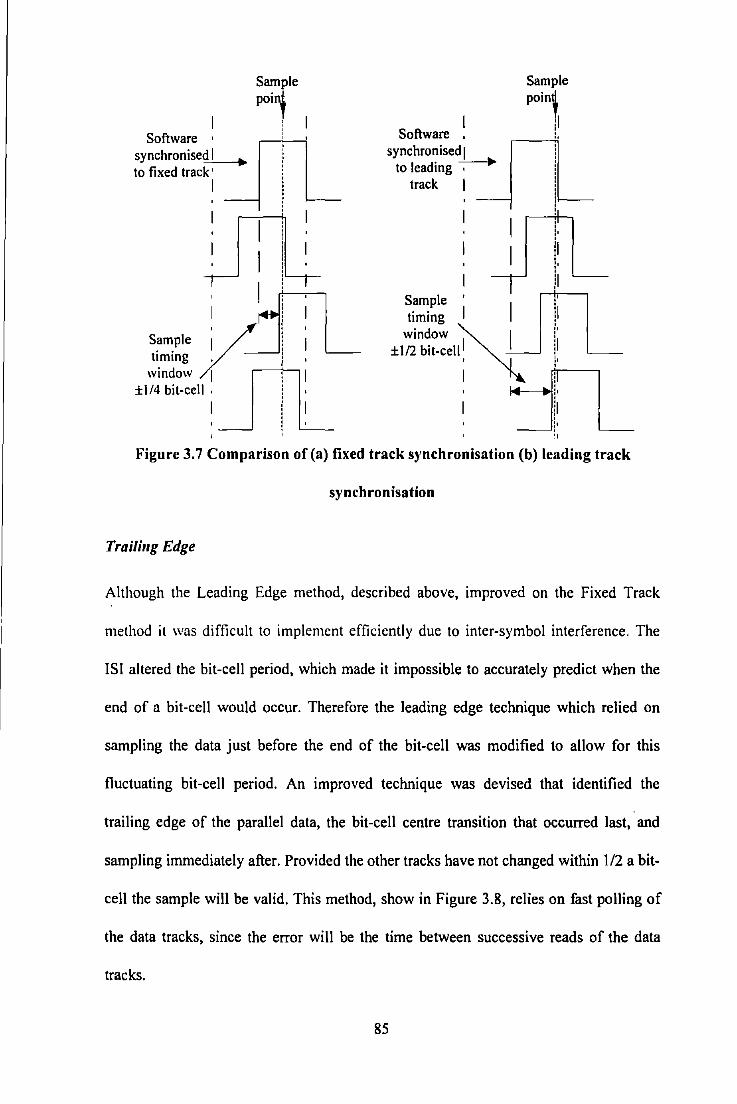
Software • synchronised=-1'----~~~o .. to fixed track'

I

Sample

poi1

' l Software synchronised 1

to leading~ track I

Sample poin\

:1 : "

Sample ' I il' timing I

window A 1. ±1/2 bit-cell: ~

Figure 3.7 Comparison of (a) fixed track synchronisation (b) leading track

synchronisation

Traili11g Edge

Although the Leading Edge method, described above, improved on the Fixed Track

method it was difficult to implement efficiently due to inter-symbol interference. The

ISl altered the bit-cell period, which made it impossible to accurately predict when the

end of a bit-cell would occur. Therefore the leading edge technique which relied on

sampling the data just before the end of the bit-cell was modified to allow for this

fluctuating bit-cell period. An improved technique was devised that identified the

trailing edge of the parallel data, the bit-cell centre transition that occurred last, and

sampling immediately after. Provided the other tracks have not changed within 1/2 a bit-

cell the sample will be valid. This method, show in Figure 3.8, relies on fast polling of

the data tracks, since the error will be the time between successive reads of the data

tracks.

85

Oversample Read

Finally to try and completely eliminate any skew-induced errors from the system's raw

error rate an oversample technique was developed. Instead of accurately timing the

length of a pulse contained on a single track and then estimating the read position to

counter the effects of skew, a timed "interrupt read' oversamples each track

individually. Each track was assigned its own software counter to time the duration of a

particular binary state. Again the ratio of time or "pulse counts" was used to determine

the position and thus the data value.

This technique, illustrated in Figure 3.8, solved several problems encountered by the

previous detection techniques, the main one being skew. By treating each track

individually skew could be completely eliminated. However, the TMS32010 could not

cope with the signal processing required to decode four tracks in real time at the data

rates required. By looking at the pulse count for each track it could be seen that as the

data rate was increased the distribution of the pulse counts spread. This method was able

to highlight the fact that data could be detected up to about 7 kbits/sec/track, beyond this

point inter-symbol interference becomes predominant and makes it almost impossible to

determine 2:1 & 1 :2 ratios from 1:1 ratios.

86

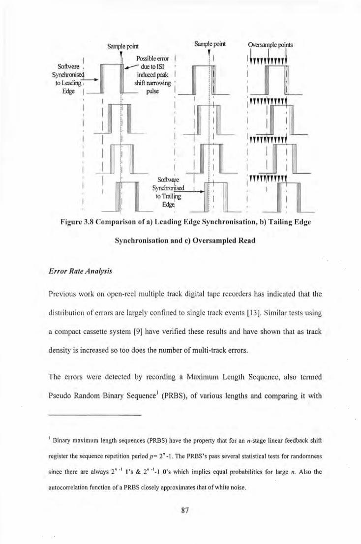
I Sofuwre 1

Synchronised to~~

Edge

Sample point

~ Possible error .....--..m_.-- d~ to ISI

induced peak shift narrowing I

pulse I

Sample point

r ~ ! :

! I I

! I

'

! i

Oversample points

tnntnn~

IL '""'"" I I

I THHI HHT

I I

Figure 3.8 Comparison of a) Leading Edge Synchronisation, b) Tailing Edge

Synchronisation and c) Oversampled Read

Error Rate Analysis

Previous work on open-reel multiple track digital tape recorders has indicated that the

distribution of errors are largely confined to single track events [ 13]. Similar tests using

a compact cassette system [9] have verified these results and have shown that as track

density is increased so too does the number of multi-track errors.

The errors were detected by recording a Maximum Length Sequence, also termed

Pseudo Random Binary Sequence1 (PRBS), of various lengths and comparing it with

1 Binary maximum length sequences (PRBS) have the property that for an n-stage linear feedback shift

register the sequence repet ition period p = 2" -I. The PRBS's pass several statistical tests for randomness

since there are always 2" . J I 's & 2" ·1-1 O's which implies equal probabilities for large n. Also the

autocorrelation funct ion of a PRBS closely approximates that ofwhite noise.

87

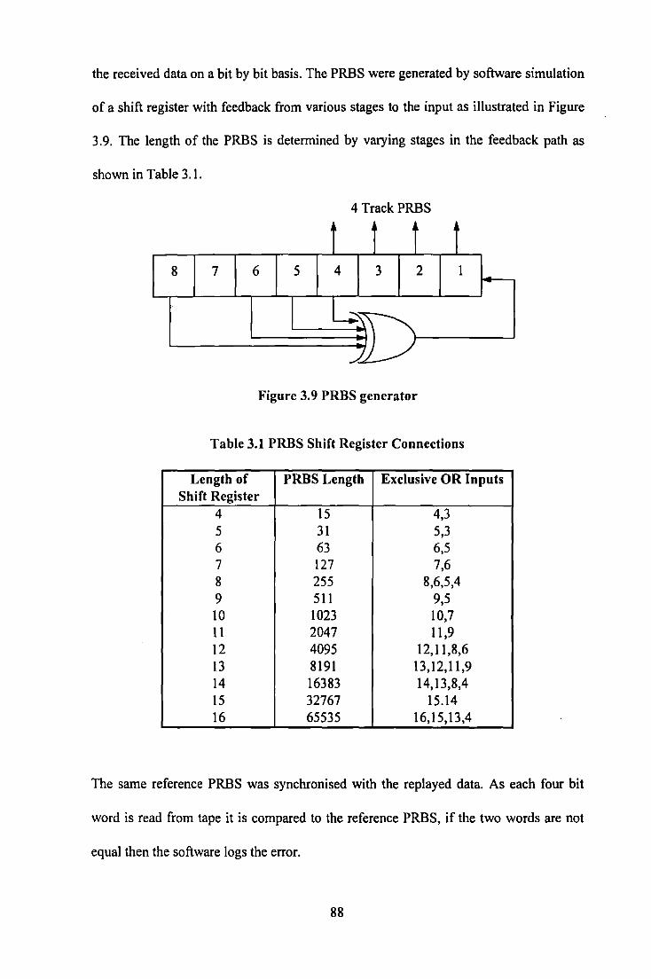
the received data on a bit by bit basis. The PRBS were generated by software simulation

of a shift register with feedback from various stages to the input as illustrated in Figure

3.9. The length of the PRBS is determined by varying stages in the feedback path as

shown in Table 3.1.

4 TrackPRBS

t t i 8 7 6 5 4 3 2 1

~\ )

j/

Figure 3.9 PRBS generator

Table 3.1 PRBS Shift Register Connections

Length of PRBS Length Exclusive OR Inputs Shift Register

4 15 4,3 5 31 5,3 6 63 6,5 7 127 7,6 8 255 8,6,5,4 9 511 9,5 10 1023 10,7 11 2047 11,9 12 4095 12,11,8,6 13 8191 13,12,11,9 14 16383 14,13,8,4 15 32767 15.14 16 65535 16, 15,13,4

The same reference PRBS was synchronised with the replayed data. As each four bit

word is read from tape it is compared to the reference PRBS, if the two words are not

equal then the software logs the error.

88

3.2.3 Experimental Procedure

Prior to operation the azimuth angle and lateral displacement of the read/write head

were set-up with the aid of a commercial Test Tone Compact Cassette tape. All tapes

were bulk erased before being used to store data. Data were not stored until a period of

20 seconds had elapsed after starting the tape to allow sufficient time for the tape leader

to pass and the tape speed to stabilise. From error rate analysis performed on the tapes it

could be seen that the section of tape following the lead-in splice was prone to a

significantly increased number of errors. This is probably due to mechanical damage

and debris deposited around the splice. The surface of the recording head, pinch roller

and capstan were cleaned using a cotton bud with Iso-Propyl Alcohol (lP A) before

recording and at regular intervals between replays.

A number of standard, commercially available compact cassette tapes were used

throughout the experimentation. In an attempt to maintain consistent results all tapes

used \vere C90, where the number relates to the total playing time of 90 minutes (45

minutes per side). Since compact cassettes tapes of different lengths have varied

thickness of polyester backing. this inevitably leads to significant differences in the

transport properties of the tape due to stretching. Apart from their playing times the

tapes used can be categorised in terms of the coercivity of their magnetic coating. The

magnetic coatings range from the low coercivity (250-350 oersted) gamma ferric oxide,

Fe20

3, to chromium dioxide, Cr02, and latterly the highest coercivity (800-1500

oersted) metal particle tapes. The higher coercivity tapes exhibit higher output and

improved frequency response compared to Fe20 3•

89

The tapes used were;

• Sony HFS 90 (Fe20 3)

• Thats TX 90 (Fe20 3)

• Maxell UDI 90 (Fe20 3)

• Maxell UDII 90 (Cr02,

• Maxell SXII 90 (Cr02,)

• Sony UX-Pro90 (Cr02,)

• Thats MG-X90 (Metal)

3.2.4 Results for System Characterisation

Initially characterisation experiments were performed to determine the optimum write

current and system bandwidth.

The write head must produce a field greater than the coercivity of the magnetic medium

in order to record information. The magnitude of the write field is dependent on the

write current. Three different types of tape coating were investigated. Each cassette tape

was recorded with a range of write currents from 0.1 mA to 2mA and the signal

amplitude of the replayed waveform was measured. Figure 3.10 illustrates how the

signal amplitude varies with write current for the coercivities of each cassette. It can be

seen that the higher the tape's coercivity the greater the maximum recorded field,

therefore the replay head will sense an increased rate of change of flux which results in

an increased magnitude replay signal.

The frequency response of the cassette system using the three different types of tape

coatings was also measured. A square wave was recorded on each cassette varying in

frequency from I OOHz to 15khz. A write current of I mA was determined to be

90

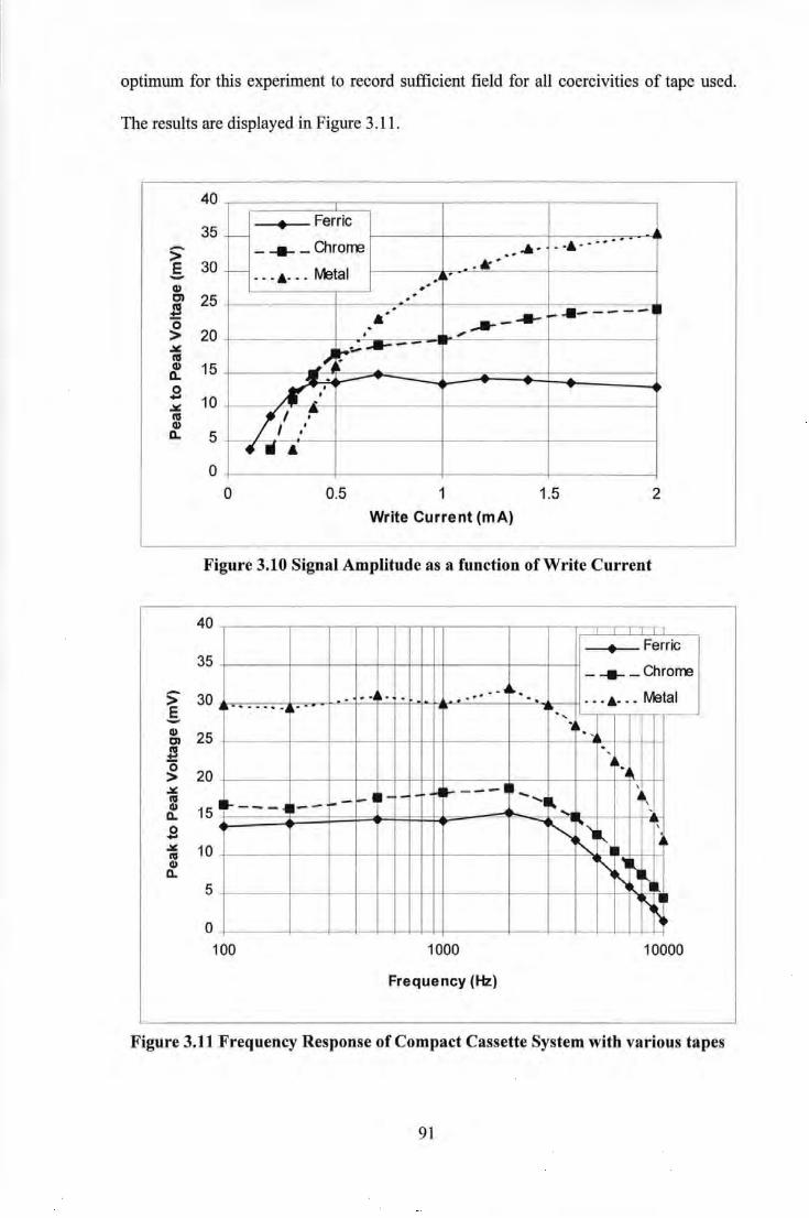
optimum for this experiment to record sufficient field for all coercivities of tape used.

The results are displayed in Figure 3.11.

40

35 -> E 30 -

• Ferric 1- --·- --... -_ --- _ Chrorre .... -· 1- ---•---1\/etal -·· . .

Q) .. C) 25 ea ... 0 > 20 .¥: ea Q) 15 0.

. . . ... -11- - - - - ·~ •• ____ .......

-• .,

.,J. ~~..----

--0 ... 10 ~ ea Q) 0. 5

f:

// fA • •

•• • 0

0 0.5 1 1.5 2

Write Current (mA)

Figure 3.10 Signal Amplitude as a function of Write Current

40

• Ferric 35 _--- _ Chrorre

- 30 > E -Cll 25 Cl

. - - - . -.. --.. .. _

. _ . •- _ • !Veta I -- - ---- -----4 . -- . , "4~. '.1

J! 0

20 > .¥: ea Cll 15 ll. 0 -.¥: 10 ea Cll ll.

5

-' 4~.

~~----· •-,. \

·~--- .. ...- -I ·-·-- ...... ·~, ·-- ' ~

~ ~1 \

~ \. \ ~ ~ ~ll ~

~ ... '\

0 100 1000 10000

Frequency (Hz)

Figure 3.11 Frequency Response of Compact Cassette System with various tapes

91

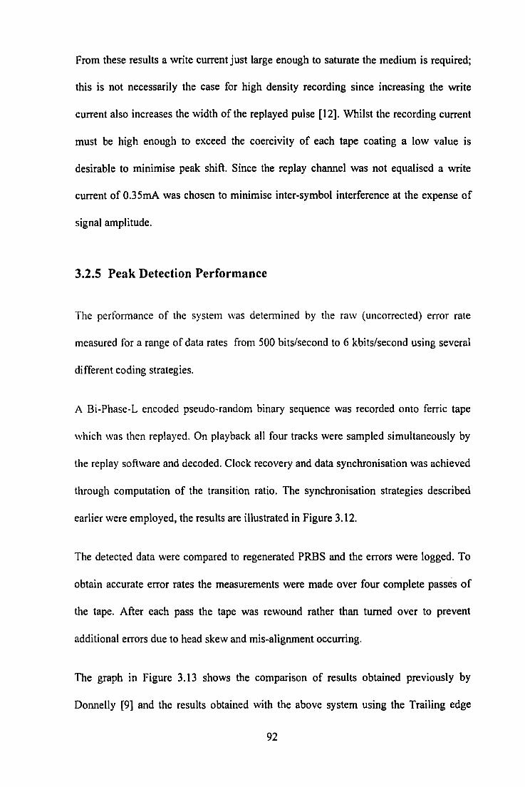
From these results a write current just large enough to saturate the medium is required;

this is not necessarily the case for high density recording since increasing the write

current also increases the width of the replayed pulse [ 12]. Whilst the recording current

must be high enough to exceed the coercivity of each tape coating a low value is

desirable to minimise peak shift. Since the replay channel was not equalised a write

current of 0.35rnA was chosen to minimise inter-symbol interference at the expense of

signal amplitude.

3.2.5 Peak Detection Performance

The performance of the system was determined by the raw (uncorrected) error rate

measured for a range of data rates from 500 bits/second to 6 kbits/second using several

different coding strategies.

A Bi-Phase-L encoded pseudo-random binary sequence was recorded onto ferric tape

which was then replayed. On playback all four tracks were sampled simultaneously by

the replay software and decoded. Clock recovery and data synchronisation was achieved

through computation of the transition ratio. The synchronisation strategies described

earlier were employed, the results are illustrated in Figure 3.12.

The detected data were compared to regenerated PRBS and the errors were logged. To

obtain accurate error rates the measurements were made over four complete passes of

the tape. After each pass the tape was rewound rather than turned over to prevent

additional errors due to head skew and mis-alignment occurring.

The graph in Figure 3.13 shows the comparison of results obtained previously by

Donnelly [9] and the results obtained with the above system using the Trailing edge

92

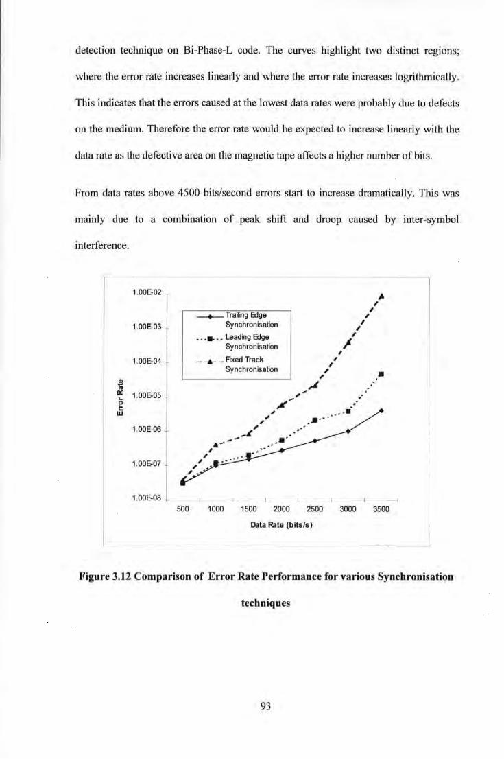
detection technique on Bi-Phase-L code. The curves highlight two distinct regions;

where the error rate increases Linearly and where the error rate increases logrithmically.

This indicates that the errors caused at the lowest data rates were probably due to defects

on the medium. Therefore the error rate would be expected to increase linearly with the

data rate as the defective area on the magnetic tape affects a higher number of bits.

From data rates above 4500 bits/second errors start to increase dramatically. This was

mainly due to a combination of peak shift and droop caused by inter-symbol

interference.

1.00E-02 ~ ,

I -+--Trailing Edge ,

1.00E-03 Synchronisation I , ... ._ . . Leading Edge I

Synchronisation ~ , 1.00E-04 _ ......_. _ FIXed Track ,

I Synchronisation , • /

.! ,L Ill . lk:: 1.00E-05

,; . .. ~ ..... .· e . . ..

... -·· w , , ..... / 1.00E-06 .-L

, .. . ..-

1.00E-07

1.00E-08 +---t-------1~---+---+----+----+----l 500 1000 1500 2000 2500 3000 3500

Data Rate (bits/s)

Figure 3.12 Comparison of Error Rate Performance for various Synchronisation

techniques

93

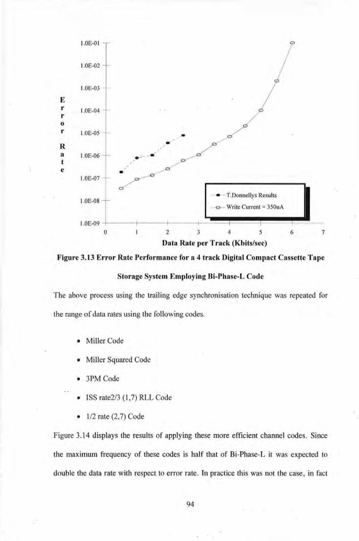
I .OE-01

I.OE-02

I.OE-03

E r I .OE-04 r 0

r I .OE-05

R a I .OE-06 t e

I.OE-07

I.OE-08

I.OE-09

0

·-- -•"' /

/

•

.-

- • - T.Donnellys Results

e--Write Current = 350uA

2 3 4 5

Data Rate per Track (Kbits/sec)

6 7

Figure 3.13 Error Rate Performance for a 4 track Digital Compact Cassette Tape

Storage System Employing Bi-Phase-L Code

The above process using the trailing edge synchronisation technique was repeated for

the range of data rates using the following codes.

• Miller Code

• MilJer Squared Code

• 3PM Code

• ISS rate2/3 ( l , 7) RLL Code

• 1/2 rate (2, 7) Code

Figure 3. 14 displays the results of applying these more efficient channel codes. Since

the maximum frequency of these codes is half that of Bi-Phase-L it was expected to

double the data rate with respect to error rate. In practice this was not the case, in fact

94

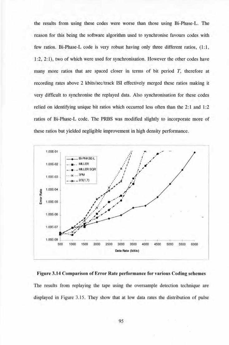
the results from using these codes were worse than those using Bi-Phase-L. The

reason for thjs being the software algorithm used to synchronise favours codes with

few ratios. Bi-Phase-L code is very robust having only three different ratios, (1: 1,

1:2, 2: 1), two of which were used for synchronisation. However the other codes have

many more ratios that are spaced closer in terms of bit period T, therefore at

recording rates above 2 kbits/sec/track ISI effectively merged these ratios making it

very difficult to synchronise the replayed data. Also synchronisation for these codes

relied on identifying unique bit ratios which occurred less often than the 2:1 and 1:2

ratios of Bi-Phase-L code. The PRBS was modified slightly to incorporate more of

these ratios but yielded negligible improvement in high density performance.

s 01 0:: ... !:! ... w

1.0013-01

1.00E-02

1.0013-03

1.0013-04 .

1.00E-05

1.00E-06

1.0013-07

... ,'1 ,

; I I --+- 81-Aii\SE-L : 1 '

; I i ·' -- --- · MLLER .' I , If

~ I , , -- • --MLLERSQR : I ,1,· ... x-.. 3PM ,.' I .1' - ~- 213(1 ,7) ... j .~:

:' ~r -~• ~~' )' ... ~ .~

,..~ ,., •' :' .· . , .. ··" -­, . .. , , . , ·' )( • .J , . ,. -, .·· . ·' , . , ·'

~ ,· ... ~~><· ... ~ ...... ,

,' .·

1.00E-06 1 --+----+- -+----+--+----+----! 500 1000 1500 2000 2500 3000 3500 4000 4500 5000 5500 6000

Data Rate (biUs)

Figure 3.14 Comparison of Error Rate performance for various Coding schemes

The results from replaying the tape using the oversample detection technique are

displayed in Figure 3. 15. They show that at low data rates the distribution of pulse

95

counts (pulse widths) is closely spaced due to little inter-symbol interference.

However at double the data rate ISI causes the distribution of pulse counts to spread.

This creates problems when trying to determine the 2: 1 and 1 :2 ratios needed for

synchronisation, since once the pulse count for a single pulse exceeds 2/3 the pulse

count for a double pulse all ratios become indistinguishable.

These results confirm the fact that for any dramatic improvement in recording density

some form of equalisation would be required in addition to azimuth correction. This

led to the design of a new system that would incorporate a more powerful DSP device

and also replace the peak detection.

96

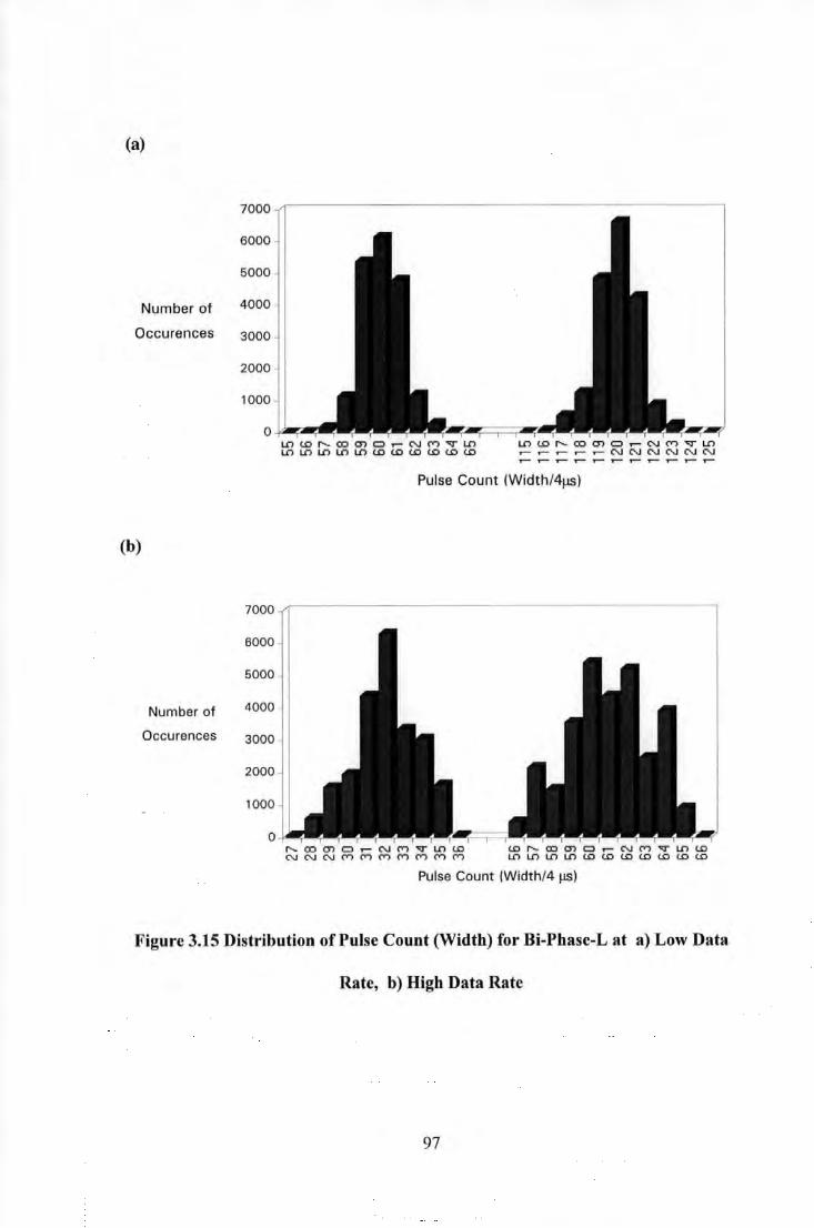
(a)

7000

6000

5000

Number of 4000

Occurences 3000

2000

1000

(b)

6000

5000

Number of 4000

Occurences 3000

2000

1000

0

LntD,...._OOO')O.-NMVLn U")L.C')U")U")U")(.O(.O(.O(.O(.O(.O

Ln<.o,...._OOO')O.-NMVLn y-~~.-r-NNNNNN r-r-r-r-,...-r-r-r-r-r-r-

Pulse Count (Width/4J..LS)

m,...._cocna.-NMVL.C'l<.o L.C')LC')L.C')LC')(.O(.D(.O(.O(.D(.D(.O

Pulse Count (Width/4 J..LS)

Figure 3.15 Distribution of Pulse Count (Width) for Bi-Phase-L at a) Low Data

Rate, b) High Data Rate

97

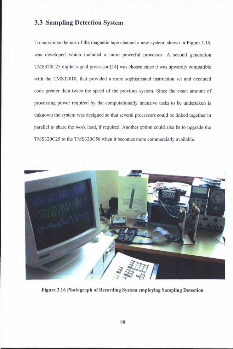
3.3 Sampling Detection System

To maximise the use of the magnetic tape channel a new system, shown in Figure 3 .16,

was developed which included a more powerful processor. A second generation

TMS320C25 digital signal processor [14] was chosen since it was upwardly compatible

with the TMS320 10, that provided a more sophisticated instruction set and executed

code greater than twice the speed of the previous system. Since the exact amount of

processing power required by the computationally intensive tasks to be undertaken is

unknown the system was designed so that several processors could be linked together in

parallel to share the work load, if required. Another option could also be to upgrade the

TMS320C25 to the TMS320C50 when it becomes more commercially available.

Figure 3.16 Photograph of Recording System employing Sampling Detection

98

3.3.1 Apparatus

TMS320C25 Processor

The TMS320C25 can execute up to 12.5 million instructions per second (MIPS) based

on a 50 MHz clock giving an instruction cycle of 80 ns. Most instructions take only one

instruction cycle. The TMS320C25 uses a 16-bit program and data word size. The

Central Arithmetic Logic Unit (CALU) has one 32-bit accumulator register and two

registers used in conjunction with the hardware multiplier. The instruction set for the

TMS320C25 contains 133 instructions, over half of which involve the CALU to

incorporate significant parallelism that speeds up DSP algorithms.

The TMS320C25 has two separate 64K-word memory spaces: program memory and

data memory. Some on-board zero wait state memory is provided in both the memory

spaces. Internal data memory consists of 544 words of RAM. Internal memory accesses

are performed using two internal 16-bit address buses and two internal 16-bit data buses.

One of each is used for program memory accesses and the other of each is used for data

memory accesses. External memory (both program and data) are accessed using a single

external 16 bit address bus and single external 16 bit data bus.

Memory addressing can be either direct or indirect. In the case of direct addressing,

memory is paged such that 128 words of data memory are addressable at any ·one

instant. Indirect addressing is provided using eight 16-bit auxiliary registers which are

also used for looping control. Seven addressing modes are provided which include two

types of address update arithmetic. One of the auxiliary registers is available as an index

register and must be shared between the seven other auxiliary registers. The Auxiliary

99

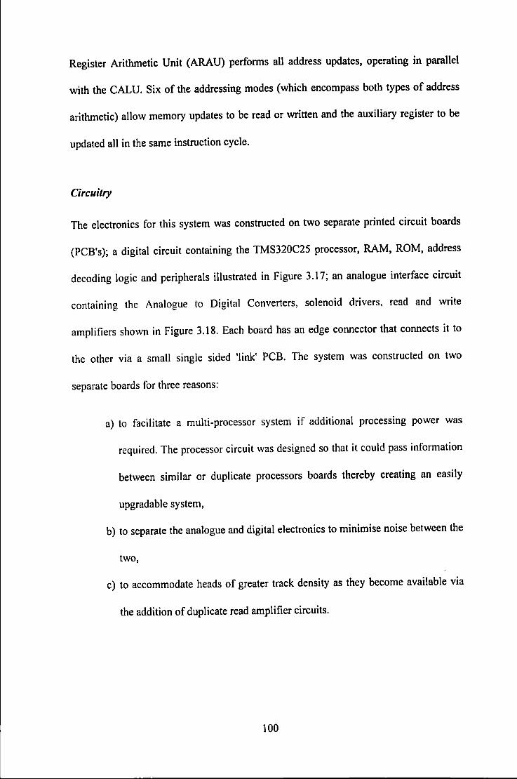
Register Arithmetic Unit (ARAU) perfonns all address updates, operating in parallel

with the CALU. Six of the addressing modes (which encompass both types of address

arithmetic) allow memory updates to be read or written and the auxiliary register to be

updated all in the same instruction cycle.

Circuitry

The electronics for this system was constructed on two separate printed circuit boards

(PCB's); a digital circuit containing the TMS320C25 processor, RAM, ROM, address

decoding logic and peripherals illustrated in Figure 3.17; an analogue interface circuit

containing the Analogue to Digital Converters, solenoid drivers, read and write

amplifiers shown in Figure 3.18. Each board has an edge connector that connects it to

the other via a small single sided 'link' PCB. The system was constructed on two

separate boards for three reasons:

a) to facilitate a multi-processor system if additional processing power was

required. The processor circuit was designed so that it could pass information

between similar or duplicate processors boards thereby creating an easily

upgradable system,

b) to separate the analogue and digital electronics to minimise noise between the

two,

c) to accommodate heads of greater track density as they become available via

the addition of duplicate read amplifier circuits.

lOO

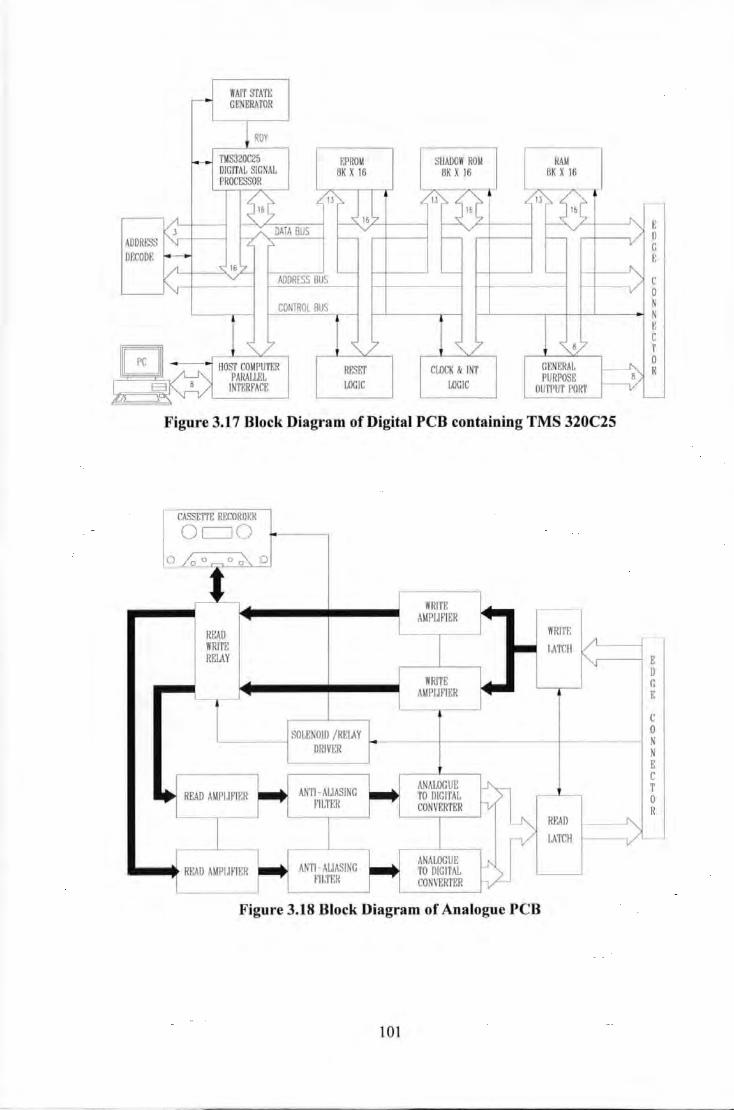
Figure 3.17 Block Diagram of Digital PCB containing TMS 320C25

CASSE'ITE RECORDER

Oc=JO 0 / 0 o .-. o 0'\_ 0

t WRITE

~ AMPLIFIER

REAI.l WRITE

~ ,-

WRITE ~ IATCII RELAY E

ll WRITE

~ G IUIPUFIER E

c SOLENOID / RElAY 0

N DRIVER N

'--- - E

~ c

• ... AN1HLIASING ... ANALOGUE T READ AMPI.IF'IER TO DIGITAL.

FILTER CONVERTER 0 R

;> READ ~ lATCH L__ ... ANTI -AI.JASI 'G ~

ANALOGUE

~ READ AMPI.Jf'IER TO DIGITAL FILTER CONVERTER

Figure 3.18 Block Diagram of Analogue PCB

101

Write Amplifier

Since the bandwidth of the write amplifier is limited by the time constant of the write­

head inductance and its series resistance, the write amplifier used in the first system

experienced a poor rise-time. This could be improved in two ways: either increase the

voltage across the head and series resistor to increase the rise time or increase the series

resistor to improve the time constant. Several circuits adopting one or both of the

improvements were designed and tested. The circuit finally chosen sacrificed optimum

performance for simplicity. This circuit makes use of the MC1488 quad line driver,

which converts standard TTL input logic levels of Ov and 5v through one stage of

inversion to output levels of+ 12v and -12v respectively. Therefore a single, low cost,

chip can provide two write amplifiers with the addition of some series resistors.

Digital "Sampling" Detector

The term sampling detector is used here to denote the detection method that samples the

read-head output with an analogue-to-digital converter. The hope is that the accuracy

introduced by using sampling detection and the ensuing digital signal processing can be

used to compensate for inter-symbol interference more successfully than is possible

with peak detection, thereby increasing density. The density increases have been

verified in a number of theoretical and experimental works [3,4].

As before, each channel is pre-amplified, low pass filtered and then amplified again.

The signal is then passed through a second order anti-aliasing filter. Band limiting the

signal reduces aliasing errors caused by sampling the input signal at a rate less than

twice the highest frequency of the signal.

102

Several basic circuit configurations using operational-amplifiers are available to

perform the filtering operation. These circuits allow the choice of external components

to determine the passband characteristics and cut-off frequency of the filter. The

Infinite-Gain Multiple-Feedback (IGMF) filter was chosen since it required the fewest

external components whilst maintaining good stability. It also gives an inverted gain

and has a low output impedance.

Finally, the signal is digitised using a 10 bit analogue to digital converter (ADC) with

conversion times better than 2 f.!S, thus permitting a sampling rate of 100 ksamples/s.

3.3.2 Read Equalisation

Read equalisation was employed to improve recording density by reducing the effects of

inter-symbol interference. Since the sampling detection system digitised all the readback

signals, a digital signal processing technique was employed to slim the readback signals.

Fi11ite Impulse Respo11se (FIR) Tra11sversal Filter

Many electrical designs can produce the desired equalisation, however an efficient

equalisation method for the applied cassette tape recorder seems to be a tapped-delay­

line equaliser or transversal filter, illustrated in Figure 3.19.

The slimmed pulse as a result of the summed filter waveforms, shown in Figure 3.20,

also introduces under-shoots. These under-shoots increase in magnitude as the resultant

pulse width is reduced. If two slimmed pulses are placed in close proximity then these

under-shoots will over-lap causing interference that effectively represents high

103

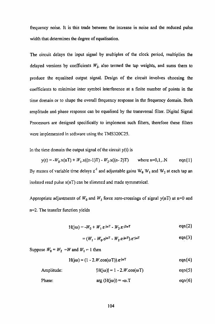
frequency noise. It is this trade between the increase in noise and the reduced pulse

width that determines the degree of equalisation.

The circuit delays the input signal by multiples of the clock period, multiplies the

delayed versions by coefficients W;, also termed the tap weights, and sums them to

produce the equalised output signal. Design of the circuit involves choosing the

coefficients to minimise inter symbol interference at a finite number of points in the

time domain or to shape the overall frequency response in the frequency domain. Both

amplitude and phase response can be equalised by the transversal filter. Digital Signal

Processors are designed specifically to implement such filters, therefore these filters

were implemented in software using the TMS320C25.

In the time domain the output signal of the circuit y(t) is

y(t) = -W0.x(nT) + W1.x((n-l)T)- W2.x((n- 2)T) where n=O,l, .. N eqn{l}

By means of variable time delays z·1 and adjustable gains W 0 W 1 and W 2 at each tap an

isolated read pulse x(nT) can be slimmed and made symmetrical.

Appropriate adjustments of W0 and W2 force zero-crossings of signal y(nT) at n=O and

n=2. The transfer function yields

HUw) = -Wo + wl.e·iOJT- Wz.e-i2ooT

= ( wl - Wo.ei"'T - Wz.e-i"'T).e·jooT

Suppose W0 = W2 =Wand W1 = 1 then

HUw) = (1 - 2. W.cos(wT)).e·iooT

Amplitude: IHUw)l = 1 - 2.W.cos(wT)

Phase: arg (HUw)) = -w.T

104

eqn{2}

eqn{3}

eqn{4}

eqn{S}

eqn{6}

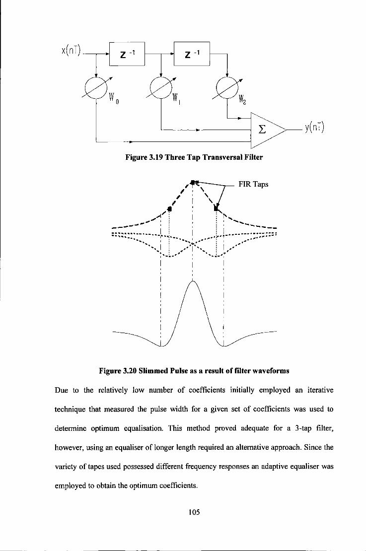
x ( n T) ------.--o.~ z -1 z -1

'>------- y( n T)

Figure 3.19 Three Tap Transversal Filter

Figure 3.20 Slimmed Pulse as a result of filter waveforms

Due to the relatively low number of coefficients initially employed an iterative

technique that measured the pulse width for a given set of coefficients was used to

determine optimum equalisation. This method proved adequate for a 3-tap filter,

however, using an equaliser of longer length required an alternative approach. Since the

variety of tapes used possessed different frequency responses an adaptive equaliser was

employed to obtain the optimum coefficients.

105

3.3.3 Adaptive Equalisation

There are a number of advantages to using an adaptive equaliser in a magnetic recording

system, in addition to the potential for density increase:

a) The channel characteristics can vary significantly with time (due to wear),

temperature and good detection schemes should adapt to such changes.

b) An adaptive equaliser can compensate for the variations in heads and

recording mediums that inevitably occur during the manufacturing process.

c) The effect of mechanical tolerances causing mis-alignment of the read head

with respect of the write head can also be minimised.

d) An adaptive equaliser can significantly reduce maintenance and installation

costs by eliminating the need for individual product adjustment, which are

instead performed automatically by the equaliser.

e) Finally, an appropriately modified adaptive equaliser can compensate for

non-linear and data-dependent noise effects that can not be accurately

anticipated or eradicated in a fixed design.

The adaptive equaliser, shown in Figure 3.21 consists of two distinct parts; a digital

transversal filter with adjustable coefficients and an adaptive algorithm which is used to

modify the coefficients of the filter. In 1960 Widrow and Hoff [16] presented a Least­

Mean-Squared (LMS) error algorithm for general purpose adaptive filtering, when a

training sequence is available. Lucky [17] further observed that once reliable decisions

are available at the receiver output, these decisions could replace the training sequence

106

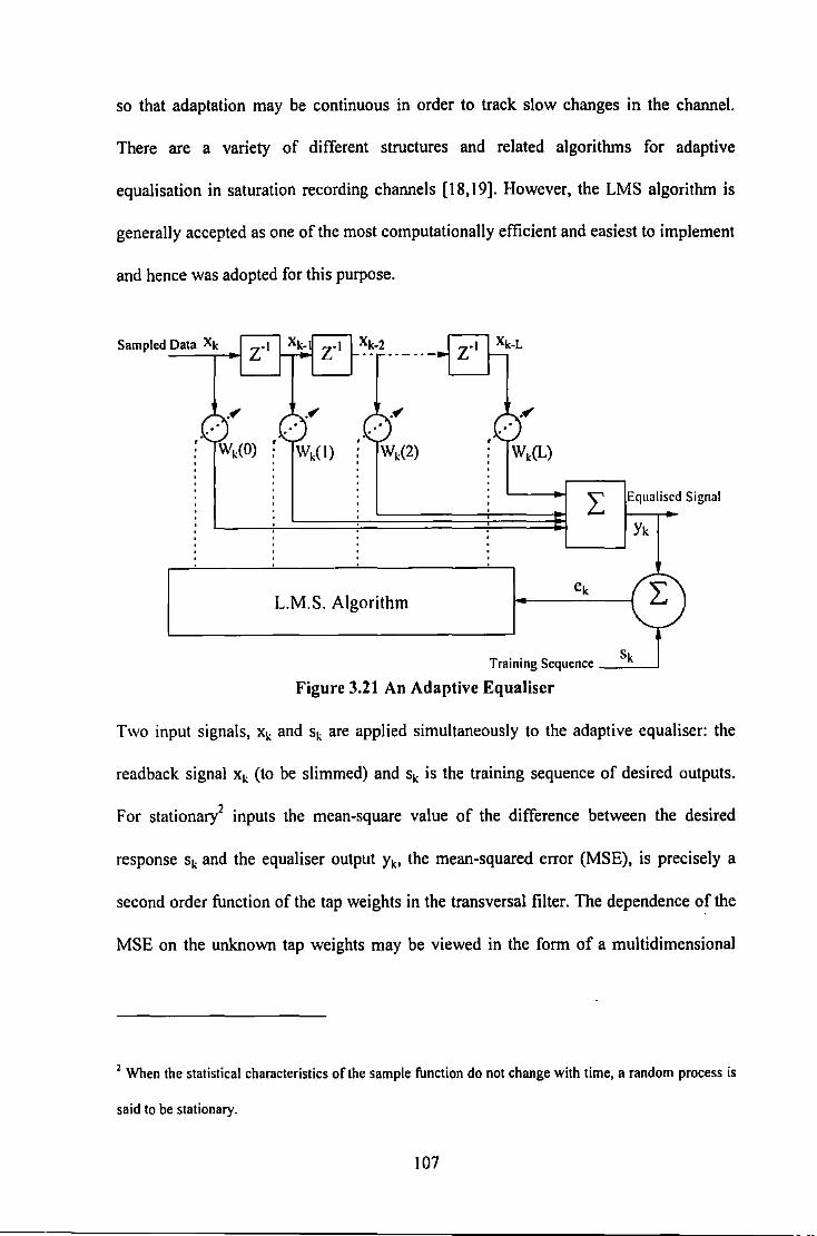
so that adaptation may be continuous in order to track slow changes in the channel.

There are a variety of different structures and related algorithms for adaptive

equalisation in saturation recording channels [18, 19]. However, the LMS algorithm is

generally accepted as one of the most computationally efficient and easiest to implement

and hence was adopted for this purpose.

Sampled Data Xk

L.M.S. Algorithm

L Equalised Signal

Yk

sk Training Sequence -~__J

Figure 3.21 An Adaptive Equaliser

Two input signals, xk and sk are applied simultaneously to the adaptive equaliser: the

readback signal xk (to be slimmed) and sk is the training sequence of desired outputs.

For stationar/ inputs the mean-square value of the difference between the desired

response sk and the equaliser output Yk• the mean-squared error (MSE), is precisely a

second order function of the tap weights in the transversal filter. The dependence of the

MSE on the unknown tap weights may be viewed in the form of a multidimensional

2 When the statistical characteristics of the sample function do not change with time, a random process is

said to be stationary.

107

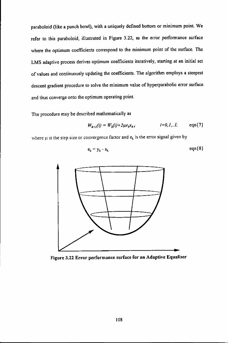
paraboloid (like a punch bowl), with a uniquely defined bottom or minimum point. We

refer to this paraboloid, illustrated in Figure 3.22, as the error performance surface

where the optimum coefficients correspond to the minimum point of the surface. The

LMS adaptive process derives optimum coefficients iteratively, starting at an initial set

of values and continuously updating the coefficients. The algorithm employs a steepest

descent gradient procedure to solve the minimum value of hyperparabolic error surface

and thus converge onto the optimum operating point.

The procedure may be described mathematically as

Wk+li) = Wli)+ 211e,.xk-l i=O,l, .. L

where ~~ is the step size or convergence factor and ek is the error signal given by

Figure 3.22 Error performance surface for an Adaptive Equaliser

108

eqn{7}

eqn{S}

3.3.4 Results for Pulse Slimming

A simple 3-tap FIR filter was implemented to equalise the channel by slimming the

pulse. The resultant waveform shown in Figure 3.23 is approximately 20% slimmer

than the original playback signal.

Isolated Pulse

... ---

_ ... ,..

, I

I I

I

~ I , _,

I , ' ' '

FIR Taps

........... ..... _ ----

Figure 3.23 Isolated Lorentzian Pulse Slimmed with a 3-tap Transversal Filter

Since the replay signal is not a perfect Lorentzian pulse it is necessary to increase the

length of the filter to improve the response. By oversampling the readback signal at

100 k.samples/sec. and employing a 5-tap filter it was possible to slim the pulse by

approximately 30%.

At high recording densities3 the readback signal is the linear super-position of the

isolated pulses. Figure 3.24 illustrates how, at these high densities, ISI causes errors

3 A data rate of 5.5 kbits/s/track using Bi-phase-L code translates to a recording density, PW50/T=3.9,

where T is the minimum time between transitions.

109

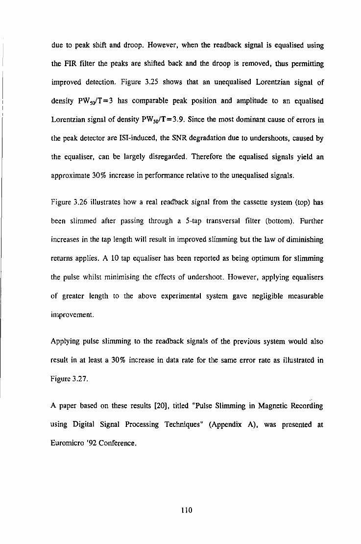
due to peak shift and droop. However, when the readback signal is equalised using

the FIR filter the peaks are shifted back and the droop is removed, thus permitting

improved detection. Figure 3.25 shows that an unequalised Lorentzian signal of

density PW 5ofT= 3 has comparable peak position and amplitude to an equalised

Lorentzian signal of density PW50/T=3.9. Since the most dominant cause of errors in

the peak detector are !SI-induced, the SNR degradation due to undershoots, caused by

the equaliser, can be largely disregarded. Therefore the equalised signals yield an

approximate 30% increase in performance relative to the unequalised signals.

Figure 3.26 illustrates how a real readback signal from the cassette system (top) has

been slimmed after passing through a 5-tap transversal filter (bottom). Further

increases in the tap length will result in improved slimming but the law of diminishing

returns applies. A 10 tap equaliser has been reported as being optimum for slimming

the pulse whilst minimising the effects of undershoot. However, applying equalisers

of greater length to the above experimental system gave negligible measurable

improvement.

Applying pulse slimming to the readback signals of the previous system would also

result in at least a 30% increase in data rate for the same error rate as illustrated in

Figure 3.27.

--

A paper based on these results [20]. titled "Pulse Slimming in Magnetic Recording

using Digital Signal Processing Techniques" (Appendix A), was presented at

Euromicro '92 Conference.

110

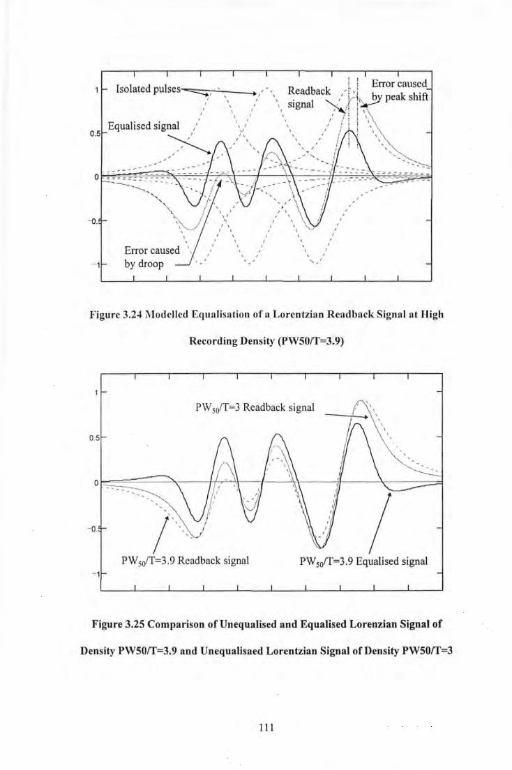
-o.

Isolated pulses-~=::~,~--....... / \ I \ \

' Equalised signal ,'

~

Error caused by droop

\

I

I\

I I

' I

' '

I

I

signal I

\ I

'

\

' \ 'I I

I

I

I

' '

Figure 3.24 l\lodelled Equalisation of a Lorentzian Read back Signal at High

Recording Density (PW50rf=3.9)

PW 5ofT=3 Read back signal

-o.

PW5ofT=3.9 Readback signal

Figure 3.25 Comparison of Unequalised and Equalised Lorenzian Signal of

Density PW50rf=3.9 and Unequalisaed Lorentzian Signal of Density PW50rf=3

111

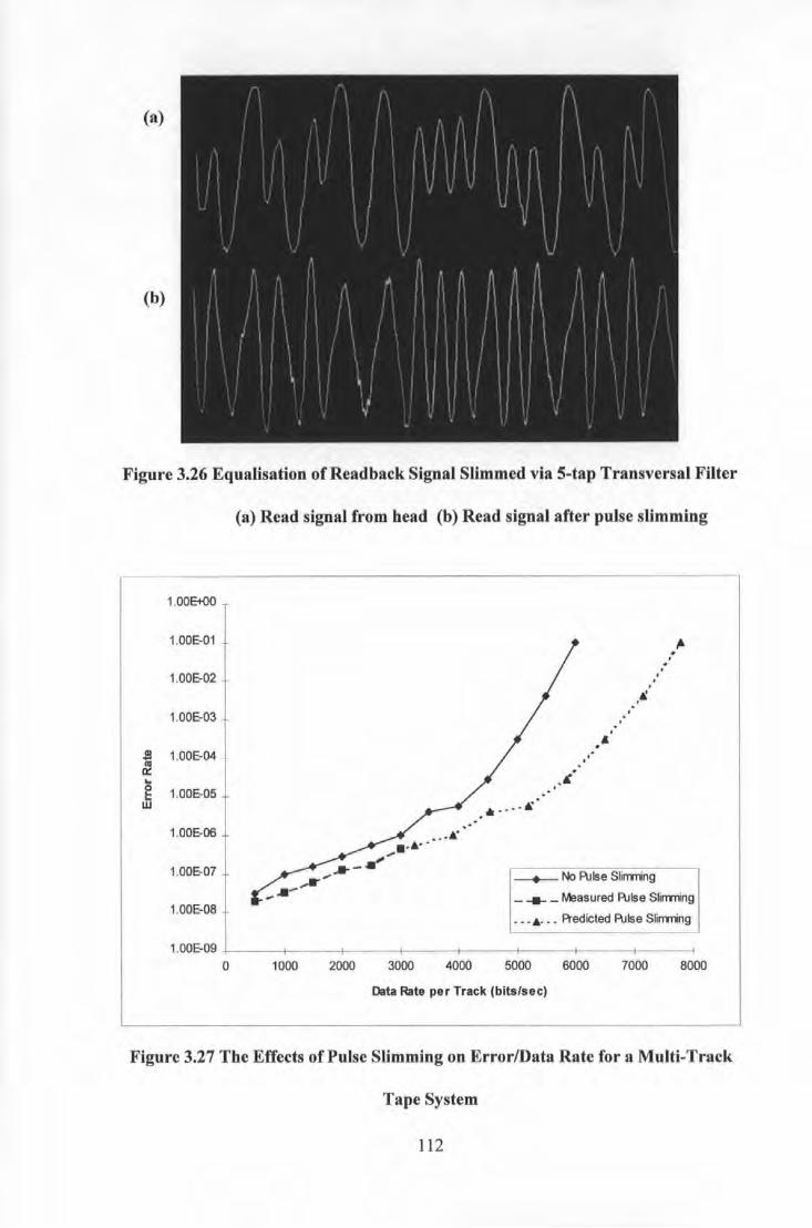
(a)

(b)

Figure 3.26 Equalisation ofReadback Signal Slimmed via 5-tap Transversal Filter

1.008{)0

1.00E-01

1.00E-02

1.00E-03

s ~ 0::

1.00E-04

.. 0 .. .. 1.00E-05 w

1.00E-06

1.00E-07

1.00E-08

1.00E-09

0

(a) Read signal from head (b) Read signal after pulse slimming

... ·-1000

....r"

••••• ;" .... -•

2000 3000

.. ···•·

4000

.-"· • ..•. ji·

. .

. ~ . .

---+--- No F\Jise S~rrrring

. . . . ~

_ _.... _l\feasured Pulse Slirrrring

• •• A· .• A-edicted F\Jise Slirrrring

5000 6000 7000 8000

Data Rate per Track (bits/sec)

Figure 3.27 The Effects of Pulse Slimming on Error/Data Rate for a Multi-Track

Tape System

112

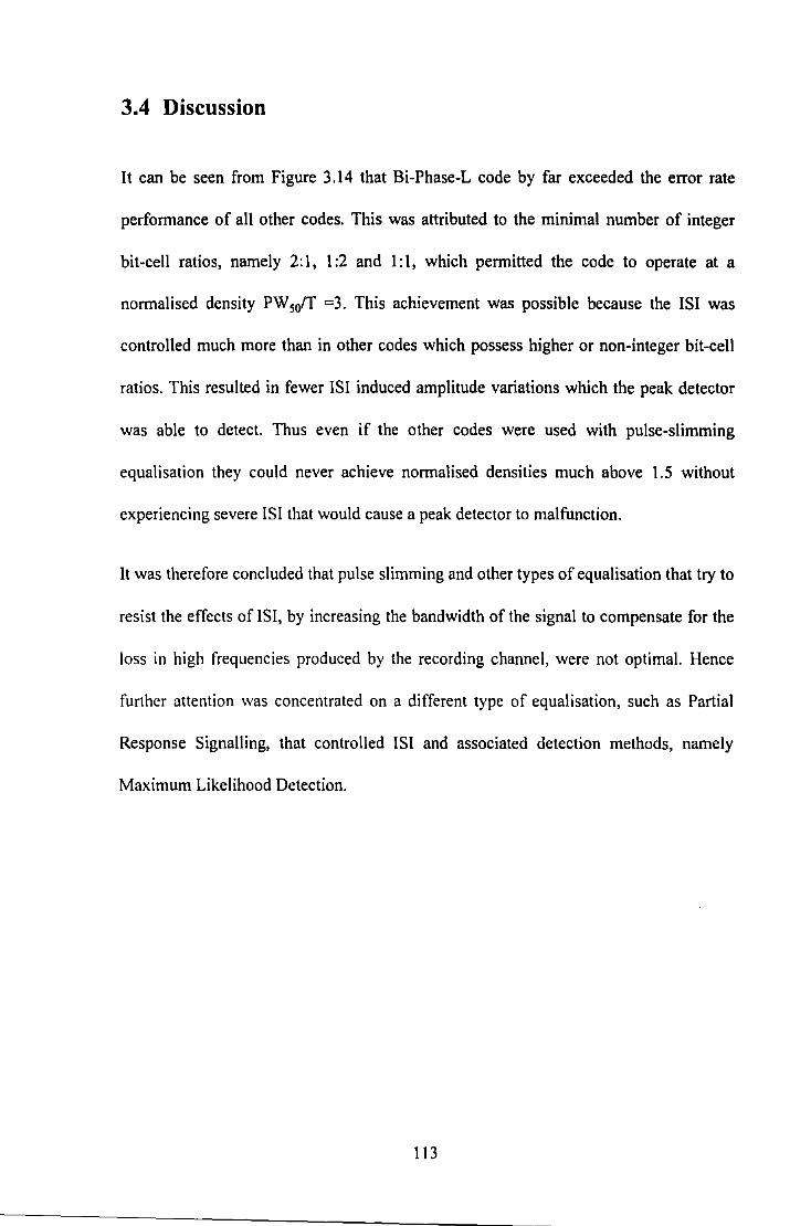
3.4 Discussion

It can be seen from Figure 3.14 that Bi-Phase-L code by far exceeded the error rate

performance of all other codes. This was attributed to the minimal number of integer

bit-cell ratios, namely 2:1, 1 :2 and 1:1, which permitted the code to operate at a

normalised density PW50ff =3. This achievement was possible because the ISI was

controlled much more than in other codes which possess higher or non-integer bit-cell

ratios. This resulted in fewer ISI induced amplitude variations which the peak detector

was able to detect. Thus even if the other codes were used with pulse-slimming

equalisation they could never achieve normalised densities much above 1.5 without

experiencing severe IS! that would cause a peak detector to malfunction.

It was therefore concluded that pulse slimming and other types of equalisation that try to

resist the effects of ISI, by increasing the bandwidth of the signal to compensate for the

loss in high frequencies produced by the recording channel, were not optimal. Hence

further attention was concentrated on a different type of equalisation, such as Partial

Response Signalling, that controlled ISI and associated detection methods, nan1ely

Maximum Likelihood Detection.

113

3.5 References

l. Mackintosh, N.D., "The Choice of a Recording Code", IERE Conf. on Video &

Data Recording, pp.77-119, 24-27 July 1979.

2. Graham, I.H., "Data Detection Methods vs Head Resolution in Digital Magnetic

Recording", IEEE Trans. Magn., Vol.14, No.4, pp.191-93, July 1978.

3. Moon, J.J., & Carely, L.R., "Performance Comparisons of Detection Methods in

Magnetic Recording", IEEE Trans. Magn., Vol.26, No.6, pp.3155-72, November

1990.

4. Nakagawa, S., et al., "A Study on Detection Methods of NRZ Recording", IEEE

Trans. Magn., Vol.MAG-16, No.1, pp.l04-10, January 1980.

5. Deeley, E.M., "Integrating & Differentiating Channels in Digital Tape Recording

IERE Journal, Vo1.56, No.4, ppl69- 73, 1986.IERE Journal, Vol.56, No.4,

pp 169- 73, 1986.

6. Siege!, P.H., "Application of a Peak Detection Channel", IEEE Trans. Magn.,

Vol.16, No.6, pp.1250-52, November 1982.

7. 'TMS320 10 User's Guide", Texas Instruments, 1983.

8. Donnelly, T., Mapps, D.J., & Wilson, R., "An Intelligent Microprocessor Interface

for a Low-Cost Digital Magnetic Tape Recorder", Microprocessing and

Microprogramming, 22(1988), pp.333-338.

9. Donnelly, T., "Real-time Microprocessor Techniques for a Digital Multitrack

Tape Recorder", Phd Thesis, Plymouth Polytechnic, 1989.

10. "Turbo Pascal User's Guide", Borland, 1990.

114

11. Smithson, P., "DSP-Based Clock Recovery for a Digital Magnetic Data Channel",

submitted to Globecom '94 (San Francisco, CA), 1994.

12. Bellis, F.A., "Introduction to Digital Audio Recording", !ERE Radio & Electronic

Eng., Vol.53, No.lO, pp.361-68, October 1983.

13. Devereux, M.A., "Error Protection Techniques for Longditudinal Digital

Recording of Audio and Video Signals", BBC Research Report, BBC/RD

1979/30, December 1979.

14. "TMS320C25 User's Guide", Texas Instruments, 1986.

IS Troullinos, G., & Bradley, J., "Hardware interfacing to the TMS320C25- Product

Application", Texas Instruments,

16. Widrow, B., & Hoff, M.E.J., "Adaptive Switching Circuits", IRE 1960 Wescon

Conv. Record, pp.563-587, 1960.

17. Lucky, R.W., Salz, J., Weldon, E.J., "Principles of Data Communications",

McGraw Hill, 1968.

18. Cioffi, J.M., Abbott, W.L., & Fisher, K.D., "Survey of Adaptive Equalization for

Magnetic Disk Storage Channels", Asilomar 22nd Conf. on Signals, Systems &

Computers, Vol. I, pp.20-24, 1988.

19. Cioffi, J.M, Abbott, W.L., Thapar, H.K., Melas, C.M., & Fisher, K.D., "Adaptive

Equalization in Magnetic Disk Storage Channels", IEEE Comms. Magazine,

Vol.28, No.2, pp.14-29, Febuary 1990.

20. Davey, P.J., Donnelly, T., & Mapps, D.J., "Pulse Slimming in Magnetic

Recording using Digital Signal Processing Techniques", Microprocessing and

Microprograrnrning, Vol.37, pp. 73-76, 1993.

115

CHAPTER4

Increased Recording Density using One

Dimensional Coding Techniques

4.1 Introduction

In conventional magnetic recording channels employing peak detection, RLL

constrained codes have played a crucial role in achieving maximum linear bit density

with low error rate. The (d. k) constraints reduce inter-symbol interference whilst

ensuring adequate self-clocking characteristics of the data signal. Recently, a different

approach to combating ISI, referred to as PRML (Partial Response (PR) signalling with

Maximum Likelihood (ML) sequence detection) has demonstrated increased storage

potential. Therefore, a new breed of constrained codes have been developed for this

channel that limited the complexity of the computationally intensive Viterbi decoder, as

well as providing timing and gain control. Also, since PRML allows for controlled ISI,

the commonly used d constraint need not be greater than zero; indeed d = 0 allows for a

higher code rate and thus a lower clock rate for a given source data rate.

116

4.2 Maximum Likelihood Sequence Detection

Maximum Likelihood Sequence Detection (MLSD) was cited by Fomey [1] for

optimum data detection in bandlimited data communication channels. For a given

received sequence, the maximum likelihood detector selects (decodes) the output

sequence which is most likely, on the basis of observation, to have been the transmitted

sequence. An example of the complexity associated with a brute force approach to

MLSD can be achieved by realising that if L is the number of different output levels,

and N is the length of the transmitted sequence then there are LN different possible

transmitted signals. This would suggest an unreasonably complex detector since LN

likelihood values would have to be computed and compared with one another. For L=2

and N =1000 this would mean 21000 computations, an impossibly large number. The

virtue of the Viterbi Algorithm is that the number of computations necessary for MLSD

grows linearly with N rather than exponentially.

4.2.1 Viterbi Algorithm

In 1967, Viterbi [2] introduced a decoding algorithm for convolutional codes which has

since become known as the Viterbi Algorithm (V A). Omura [3] showed that the Viterbi

algorithm was equivalent to a dynamic programming solution to the problem of finding

the shortest path through a weighted graph. Fomey [4] later recognised that it was in

fact a maximum likelihood decoding algorithm for convolutional codes and pointed out

that the V A could also be used to produce the maximum likelihood estimate of the

transmitted sequence over a channel with inter-symbol interference. A comprehensive

description of the Viterbi algorithm is also given in [5].

117

This technique can be contrasted with conventional threshold detection, such as peak

detection, where valuable information is otherwise lost. Viterbi Detection is illustrated

in Figure 4.1 where an equalised playback waveform fails to cross the threshold of a

peak detector at a given point due to noise, thus resulting in erroneous data. However

by using Viterbi detection it can be seen in Figure 4.2 that the hard decisions of the

peak detector are replaced by a number of intelligent soft decisions, which result in

the correct data sequence being identified. In Viterbi detection, the signal is sampled

and its value interpreted relative to those of surrounding samples, rather than by

measuring whether the signal has crossed a threshold with a fixed value. This enables

otherwise ambiguous samples to be correctly interpreted, yielding a lower error rate

or a higher bit-packing density.

The Viterbi algorithm is simply a fast algorithm for searching a labelled trellis for a path

that most closely agrees with a given path. The V A operates iteratively frame by frame,

tracing through the trellis in the hope of finding the correct path. For each branch (path)

of the frame it computes the squared error between the received sequence and each

possible output sequence (weight). For each node (state), the branches entering the node

with the greatest cumulative weight are rejected. At any frame of the trellis the Viterbi

detector does not know which node the true data sequence has reached, nor does it try to

decode it immediately. A symbol is successfully decoded when only one survivor path

emanating from a node is remaining.

118

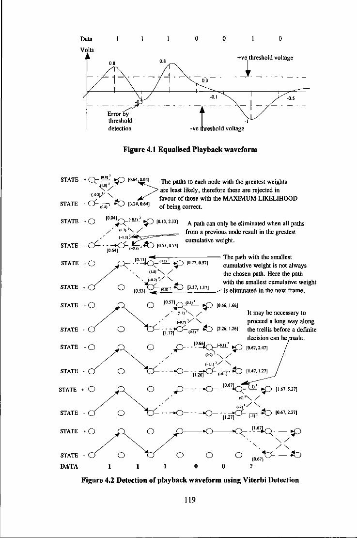
STATE

STATE

Data

Volts

-0. ---/ Error by threshold detection

0 0

Figure 4.1 Equalised Playback waveform

0

Q- (0.8)' .rJ + . -, ...-- 1°·64>0·

041 The paths to each node with the greatest weights Jl.8)/ ':- are least likely, therefore these are rejected in

(-02)/" _ cf- __ .._,_ 24

favour of those with the MAXIMUM LIKELIHOOD (D.8J' ""'-.J 13· · 0·641 of being correct.

STATE + 0 J0.04P,<~' ~ [0.13,2.33) A path can only be eliminated when all paths from a previous node result in the greatest cumulative weight.

/ • (0.7) "'- /

-~- (-1.3)~~==== STATE - cf- --0-

1_. 31 .~ (0.53,0.73]

[0.64) .

STATE

STATE

STATE

STATE

STATE

----;------- The path with the smallest +/: _[O.I~]~_(O~ ..rl (0.77,0.57) ~- ~ cumulative weight is not always '- (1.8) ., / ' the chosen path. Here the path "· <-<> 2l '/ "- with the smallest cumulative weight

- 0 (0.53J~ <08f' :tJ 13·37

• 1.171 is eliminated in the next frame.

ro.57J ~"'L ..rl ~' ~ (0.66, 1.66]

/ ' (1.3) '" /

(-<>.7) V" -- .r-/ -4--.. [2.26, 1.26) (I.I~<D.Jl' -~

It may be necessary to proceed a long way along the trellis before a defmite

rl-- - [~.66J,__ <-m' ""' ~ ~ ..-- [0.67,2.47]

/ ' (0.9) ' " /

' (-1.1)'/" STATE - - - -o{)- -[ •. 2~ (-01)' ~

STATE + 0

STATE

STATE

STATE

DATA l l

0 n- ___ .._r-.._ _ 1°·67!r._ ~ .r1 ~ ~ '"--'<, ...-- [1.67,5.27]

/ (D)'"/ ' (-2)'/" ---a----"()--- -0- ;'7.1 ~ (0.67,2.27]

(1.27] (-I)

}---o{)-~-~~·67J.q-- ~

"/ "- /"

0 0 [0.67;t:;:- - ~ 1 0 0 ?

Figure 4.2 Detection of playback waveform using Viterbi Detection

119

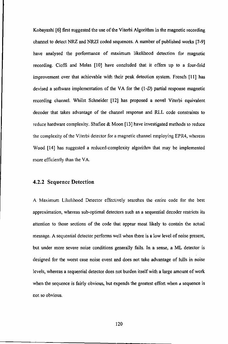
Kobayashi [6] first suggested the use of the Viterbi Algorithm in the magnetic recording

channel to detect NRZ and NRZI coded sequences. A number of published works [7-9]

have analysed the performance of maximum likelihood detection for magnetic

recording. Cioffi and Melas [10] have concluded that it offers up to a four-fold

improvement over that achievable with their peak detection system. French [ 11] has

devised a software implementation of the VA for the (1-D) partial response magnetic

recording channel. Whilst Schneider [ 12] has proposed a novel Viterbi equivalent

decoder that takes advantage of the channel response and RLL code constraints to

reduce hardware complexity. Shafiee & Moon [13] have investigated methods to reduce

the complexity of the Viterbi detector for a magnetic channel employing EPR4, whereas

Wood [14] has suggested a reduced-complexity algorithm that may be implemented

more efficiently than the V A.

4.2.2 Sequence Detection

A Maximum Likelihood Detector effectively searches the entire code for the best

approximation, whereas sub-optimal detectors such as a sequential decoder restricts its

attention to those sections of the code that appear most likely to contain the actual

message. A sequential detector performs well when there is a low level of noise present,

but under more severe noise conditions generally fails. In a sense, a ML detector is

designed for the worst case noise event and does not take advantage of lulls in noise

levels, whereas a sequential detector does not burden itself with a large amount of work

when the sequence is fairly obvious, but expends the greatest effort when a sequence is

not so obvious.

120

Individual bit decisions made by a sequential detector must be considered tentatively at

each step of the decoding process. The decoder must maintain the ability to reverse any

or all of the bit decisions at a later time if it seems necessary. Sequential decoding

algorithms are thus sub-optimal tree searching procedures that share two features.

Specifically, a sequential decoder attempts to quickly recognise that it has departed from

the correct path in the code tree and uses a sequence of test criteria on path metrics to

determine the relative "correctness" of the path being pursued. A sequential decoder

attempts to find the best path in the code tree by searching for the path with the largest

metric.

Fa11o Algorithm

A very popular sequential decoding algorithm is the one developed by Fano [ 15]. This

technique can be used for hard or soft decoding . The Fano decoder searches for the

most likely transmitted message moving along the code tree one node at a time. The

direction of movement, forward or backwards, is determined by the behaviour of the

metric, therefore the selection of the metric used for sequential decoding is most crucial

for correct operation. Fano proposed the best metric function for sequential decoding is

the logarithm of the probability that a particular output is observed given that a certain

symbol was transmitted, normalised by the total probability of the observed output. The

metric suggested by Fano has the property that correct path metrics tend to increase at a

moderate rate whereas incorrect path metrics decrease relatively quickly.

121

4.3 Partial Response Signalling (Correlative Level Coding)

Nyquist [ 16] investigated the transmission of data through a bandlimited channel. He

concluded that for any bandwidth B Hz it is theoretically possible to transmit 2B

symbols/second, commonly referred to as the Nyquist Rate, without inter-symbol

interference. In other words, he showed that a maximum of B symbols/second can be

transmitted across a communication channel with a rectangular frequency response

cutting-off at B/2 Hz, the so-called Nyquist Bandwidtlr. The pulse shape required to

satisfy the Nyquist criteria is a sine (sin(x)/x) function that decays at a rate of 1/t. A

sequence consisting of sine pulses experiences considerable ISI, however the resultant

signal always pass through zero at the detection instances.

The sin(x)/x pulse shape is not practical for two main reasons:

a) The slow rate of decay makes the pulse nearly impossible to generate and

implies that extreme peak amplitudes can occur from the addition of delayed

sidelobes (tails) in phase.

b) The inter-symbol interference is only low within a small range around the

detection instances and is therefore critically dependent on accurate timing

synchronisation. Practical timing offset andjitter would generate considerable

errors.

Thus waveform design with sine pulses to make full use of the available channel

bandwidth, though mathematically simple, is impractical to implement.

122

In 1963, Lender [ 17 ,18] demonstrated that it is possible to transmit at the Nyquist rate of

2B symbols /second with no inter-symbol interference using the theoretical minimum

bandwidth ofB hertz. Lender pioneered a technique termed Duobinary signalling where

the "duo" implies the doubling ofthe transmission capacity (double the speed or half the

bandwidth) when compared to the raised cosine filter. The technique, more commonly

called Partial Response Sig11alling or Correlative Level Coding, relied on introducing a

controlled amount of ISI into the data stream rather than trying to eliminate it

completely. By introducing correlated interference between the pulses the resultant

effect "cancelled out" the interference at the detector. The term Partial Response arises

from the idea of conveying information in a channel subject to controlled amounts of

inter-symbol interference, conversely a full response assumes zero ISI. Thus the peak

detection channel previously described is a full response channel.

There are ,a p~mber of partial response schemes, categorised by Kretzmer [ 19], that are

suitable for digital communication systems. Kabal and Pasupathy [20] have produced an

excellent tutorial paper in which they define nine different partial response channels in

terms of the characterising polynomial F(D), transfer function H(ro), impulse response

h(t), and number of output signal levels. A selection of these PR schemes are given in

Table 4.1, where the system polynomials are of the form

eqn{ 1}

"

where D is the delay operator equal to one symbol delay, and/, are the sample values of

the desired impulse response that effectively define the correlation between symbols in

the information sequence.

From equation { l} the frequency response, H(ro) is obtained by substituting D = e·jwT.

123

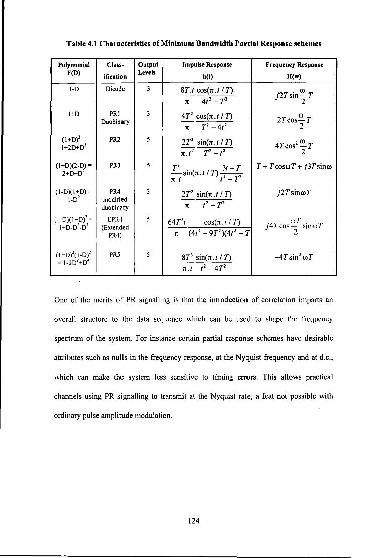
Table 4.1 Characteristics of Minimum Bandwidth Partial Response schemes

Polynomial Class- Output Impulse Response Frequency Response F(D)

ification Levels

b(t) H(w)

1-0 Oicode 3 8T.I cos(n.l IT) j2Tsin ro T 7t 41 2

- T2 2

1+0 PRI 3 4T2 cos(n .I IT) (J)

Ouobinary 2Tcos-T 7t T2 -41 2 2

(1+0)2 = PR2 5 2T3 sin(n. 1 I T) 4Tcos2 ro T 1+20+02

7t .12 rz- 12 2

(1+0)(2·0) = PR3 5 T2 . 31- T T + TcosroT + j3Tsinro 2+0+02 -sm(n.l IT) 2 2 n.l 1 -T

(1-0)(1+0)= PR4 3 2T2 sin(n.l IT) j2TsinroT 1-02 modified

duobinary 7t t2- T2

(1-0)(1"-0)2 = EPR4 5 64T3t cos(n .I I T) AT mT . T 1+0-02-03 (Extended --

(4t 2 - 9T2)(4t2 - T J cos-smro

PR4) 7t 2

(I +0/(1-0)1 PR5 5 8T3 sin(n. t I T) -4Tsin2 mT = 1-202+0

4

7t. t t 2 - 4T2

One of the merits of PR signalling is that the introduction of correlation imparts an

overall structure to the data sequence which can be used to shape the frequency

spectrum of the system. For instance certain partial response schemes have desirable

attributes such as nulls in the frequency response, at the Nyquist frequency and at d.c.,

which can make the system less sensitive to timing errors. This allows practical

channels using PR signalling to transmit at the Nyquist rate, a feat not possible with

ordinary pulse amplitude modulation.

124

The main disadvantage of partial response signalling is that it increases the number of

output levels to be larger than the number of input levels. Thus, a detector using symbol

by symbol detection will experience a reduced signal to noise ratio. Eye diagrams for

PR4 and EPR4 waveforms are shown in Figure 4.3 and Figure 4.4 respectively. These

diagrams represent the overlaying of the channel output signal seen in each time interval

T, assuming a random binary input sequence. One can clearly see the nominal three

(respectively, five level) set of values at the sampling instances for PR4 (respectively,

EPR4) response. The eye diagrams provide some useful, qualitative indication of the

robustness of the sample values at the bit cell boundaries in the presence of additive

noise and jitter.

125

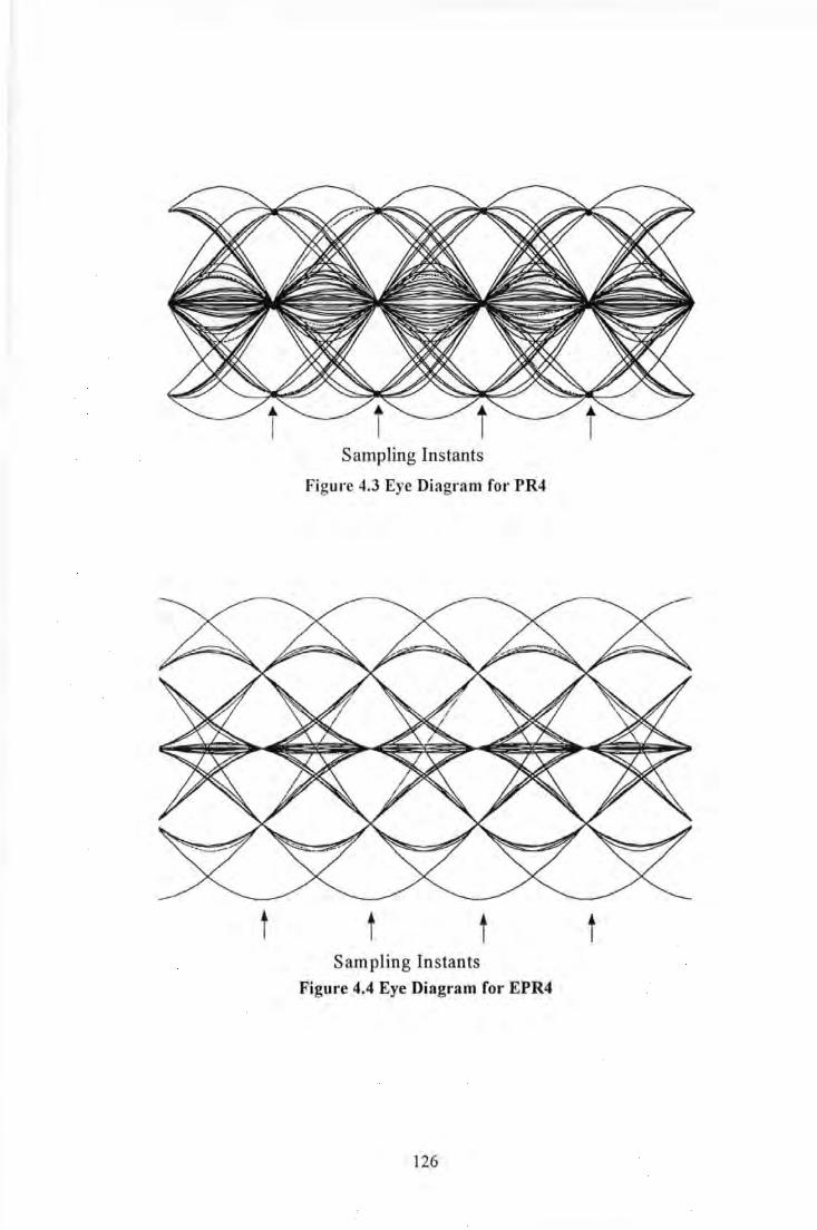
Sampling Instants

Figure 4.3 Eye Diagram for PR4

t t t t Sampling Instants

Figure 4.4 Eye Diagram for EPR4

126

4.3.1 Application to Magnetic Recording

Conventionally, partial response signalling has been considered as a transmission

technique, where the shape of the response is applied at the transmitter. However, in

magnetic recording, the channel with appropriate equalisation, is used to give the

desired pulse response. Kobayashi & Tang [21] first discovered that the step response to

a transition and the pulse response to a dibit bear close resemblance to class IV partial

response (PR4) and extended class IV partial response correlative encoding schemes.

To understand why partial response signalling applies well to magnetic recording,

consider the digital data, represented as an impulse train, is first applied to a zero order

hold circuit to form the write current in NRZ format. The write current records

transitions on the medium which are sensed by the readback process, resulting in an

analogue signal. The readback signal has a bandpass spectrum which can be

approximated by

(af)exp( -lbnl eqn{2}

where f is the frequency, and a and b are constants.

The combined transfer function of the zero order hold and the write process is similar to

the (1-D) partial response system. Thus, partial response polynomials for saturation

recording must include a (I-D) factor. Since the amplitude response of the (I-D) system

is high pass, it must, for purposes of bandwidth efficiency and spectral matching with

the overall channel transfer function, be moulded into a bandpass response. The PR4

class introduces a spectral null at the Nyquist frequency to achieve the bandpass

spectrum. The spectral requirements of the PR4 detector can be satisfied over a range of

127

recording density by suitably equalising the readback signal. Beyond that range,

however noise enhancement penalty in equalisation and the lower readback SNR, due to

the peak power limitation of the channel, cause the input SNR to the detector to drop

below the theoretical level for acceptable performance.

Thapar & Pate! [22] noted that the class of partial response systems characterised by the

following polynomial,

n P (D)=(l-D)(l+D)

n n=O, 1 ,2,3, .... eqn{3}

where P (D) defines the input-output relationship, n

are particularly suited to the magnetic recording channel.

The signal spectrum, Hn(ro), for the polynomial in equation {3} is obtained by

calculating its Fourier Transform, and this is simply achieved by substituting D=e1"'r.

which yields

eqn{4}

Figure 4.5 displays H0(ro) for a normalised frequency and various n. As shown, the

signal energy shifts towards the lower frequencies with increasing n. If, for increasing n,

the symbol interval T is reduced so that roughly the same spectral region is occupied,

the data rate (and thus the data storage density) increases correspondingly.

128

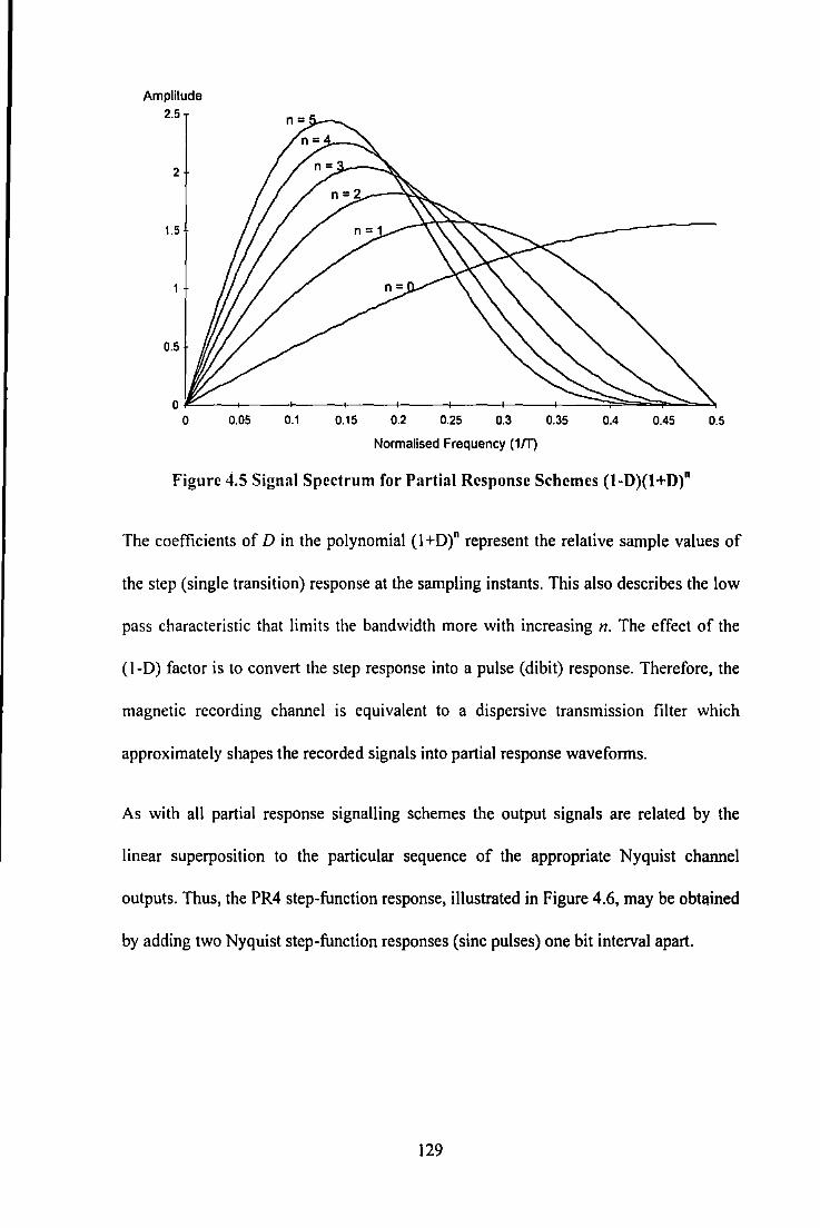
Amplitude 2.5

2

1.5

0.5

0~--~---+----~--4---~---4----+-~~~~~~ 0 0.05 0.1 0.15 0.2 0.25 0.3 0.35 0.4 0.45 0.5

Normalised Frequency (1ff)

Figure 4.5 Signal Spectrum for Partial Response Schemes (1-D)(l+D)"

The coefficients of Din the polynomial (I+D)" represent the relative sample values of

the step (single transition) response at the sampling instants. This also describes the low

pass characteristic that limits the bandwidth more with increasing n. The effect of the

( 1-D) factor is to convert the step response into a pulse (dibit) response. Therefore, the

magnetic recording channel is equivalent to a dispersive transmission filter which

approximately shapes the recorded signals into partial response waveforms.

As with all partial response signalling schemes the output signals are related by the

linear superposition to the particular sequence of the appropriate Nyquist channel

outputs. Thus, the PR4 step-function response, illustrated in Figure 4.6, may be obtained

by adding two Nyquist step-function responses (sine pulses) one bit interval apart.

129

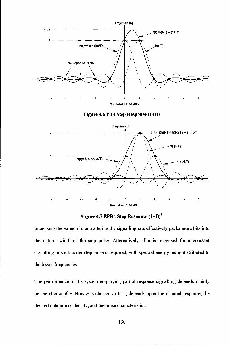
Amplitude (A)

1.27-------

1---I

h(t)=A slnc(ntfT)~/

I

Sampling Instants

I ~ __ \ __ , --- ,.,. .... --~....... .... ...... ----....... ,/"' ' ,.. \ .... ----.......... - ... _____ .... ... ... _, ........ ___ ........ .... ....... __ ....... ' ....... ____ ....... ... ...... ___ .... "

' .... _../'

-5 -3 -2 -1 0 2 3 4

Nonnallaed nme (UT)

Figure 4.6 PR4 Step Response (1 +D)

Amplitude tAl

2------

1--h(t)=A sinc(nVT)

.......... -- ...... .... ____ , =:::::=.::. ... :;:- ... -- / ' _____ ..

-5 -4 -3 -2 -1

' ' ,_/

0

Nonnallsed nme (UT)

h!tJ+2h!t-n+h(t-2n = 11 +D2J

/

2h!t-n

\ / ' ... ===/:;;: ....... __ ............

2

\ ' './

3 4

Figure 4. 7 EPR4 Step Response (1 +D)2

5

-'t::;:==

5

Increasing the value of n and altering the signalling rate effectively packs more bits into

the natural width of the step pulse_ Alternatively, if n is increased for a constant

signalling rate a broader step pulse is required, with spectral energy being distributed to

the lower frequencies_

The performance of the system employing partial response signalling depends mainly

on the choice of n. How n is chosen, in turn, depends upon the channel response, the

desired data rate or density, and the noise characteristics.

130

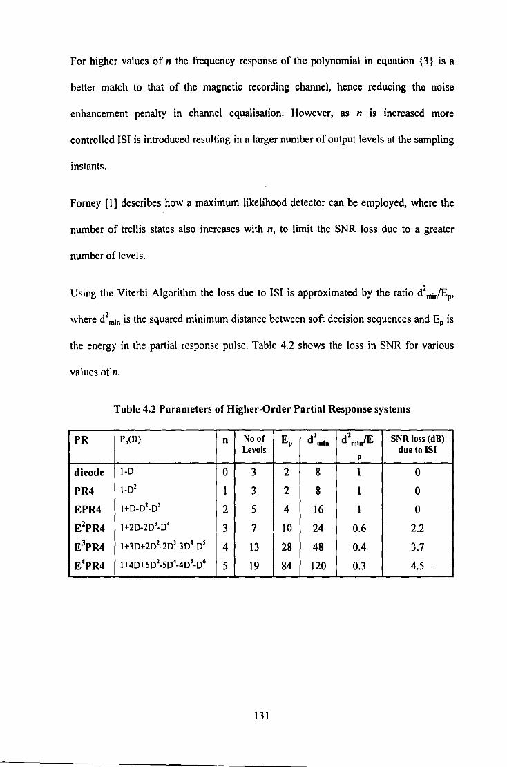
For higher values of n the frequency response of the polynomial in equation {3} is a

better match to that of the magnetic recording channel, hence reducing the noise

enhancement penalty in channel equalisation. However, as n is increased more

controlled ISI is introduced resulting in a larger number of output levels at the sampling

instants.

Fomey [I] describes how a maximum likelihood detector can be employed, where the

number of trellis states also increases with n, to limit the SNR loss due to a greater

number of levels.

Using the Viterbi Algorithm the loss due to ISI is approximated by the ratio d2 mi,/Ep,

where d2 min is the squared minimum distance between soft decision sequences and EP is

the energy in the partial response pulse. Table 4.2 shows the loss in SNR for various

values ofn.

Table 4.2 Parameters of Higher-Order Partial Response systems

PR P.(D) No of EP 1 2 SNR loss (dB) n d min d min/E

Levels due to JSJ p

dicode 1-0 0 3 2 8 1 0

PR4 1-02 1 3 2 8 1 0

EPR4 1+0-02-03 2 5 4 16 1 0

E1PR4 1+20-203-04 3 7 10 24 0.6 2.2

E3PR4 I +30+202-203 -304-05 4 13 28 48 0.4 3.7

E4PR4 I +40+502-504-405-06 5 19 84 120 0.3 4.5

131

4.4 PRML Coding

4.4.1 Precoding

Precoding is a non-redundant transformation on a bit stream prior to entering a channel

that cancels another transformation that takes place on the bit stream within the channel

(or modulator/demodulator). The cascade of the precoder and the channel will return the

binary sequence to its original form.

This technique is used to alleviate error propagation at the decoder by eliminating the

effect of previous symbols at the source where they are known precisely. In essence this

is equivalent to making the decoder memoryless.

For instance, the recorded binary sequence ak replayed through a magnetic recording

channel equalised to PR4 (l-D2), shown in Figure 4.8, can be represented by

eqn{5}

Therefore each transmitted symbol is correlated with a prior symbol which suggests that

the original binary recorded sequence can be decoded as

. . . a k = c k +a k·2 eqn{6}

From this equation it can be seen that if noise corrupts c·k then not only will a·k b~ in

error but so also will a· k+2, a \+4, a· k+6•···

Figure 4.9 illustrates how Lender [23] cleverly solved this problem by introducing a

precoder, using modulo-2 arithmetic, that has a transfer function equal to the inverse of

the channel.

132

" {c d

{ad

+

+

+

PR4 Channel (1-D1)

2D {ad 0 0 0 1 0 1 0 0 1 1 1 1 0 0 0

\! { ck} 0 1 0 0 0 -1 1 1 0 0 -1 -1

Detector " {ad

A A A

a k= c k +a k-2

2D {cAd 0 0 0 1

~i 0 0 0-1 0 1 0 0-1 -1 a k-2 L----'

{a\} 0 0 0 1 0 1 0 0 0 1 0 1 1 0

\ t I Error Propagates

Figure 4.8 Propagation of Errors in PR4 channel

{bd +

2D 2D b k-2 L---___.J

Precoder (lll-D2)

L___ _ _jbk-2

PR4 Channel (1-D2

)

{~} 0 0 0 1 0 1 0 0 1 1 1 1 0 0 0

{bd 0 0 0 1 0 0 0 0 1 1 0 0 0 0 0

/

Error A without Propagation

{ad 0 0 0 1 0-1 0 0 0 1 -1 -1 0 0 0

Figure 4.9 Use of Precoder to prevent Error Propagation

133

4.4.2 Randomisation

Early attempts at applying partial response and maximum likelihood detection to the

magnetic recording channel involved the use of data randomisation [24, 25]. As

described in chapter 2, randomisation or scrambling is a non-redundant technique

employed to alleviate undesirable properties of the source data, e.g., d.c. content, and

long run lengths. This coding technique was also employed in the first known

commercial product to employ PRML [26-28], a "black box" flight recorder produced

by Ampex.

The main reason this method of coding was chosen instead of a conventional l/2 rate

RLL codes [29,30], was to enable the channel to be considered as two interleaved (l-D)

channels. Thus allowing the Viterbi detector to be split into two independent detectors,

that could proceed completely separately on the two, odd and even, data streams. From

this separation three distinct advantages accrue:

a) Both data streams can be processed at one-half the data rate. At high data

rates this is a vital consideration and is in sharp contrast to the Viterbi

detection of Miller Squared code [31] where similar processing must proceed

at twice the source data rate.

b) The channel memory which determines the complexity of the Viterbi detector

is halved.

c) Two-state detectors are more easily implemented than detectors involving an

increased number of states such as would be required for a single Viterbi

detector [32].

134

4.4.3 (0, G/1) Codes

The previous section highlights the advantages in Viterbi detection by considering the

PR4 channel to be two interleaved (1-D) channels. This group of codes was specifically

designed for this type of channel implementation.

In a PRML channel, a channel code can also be used to provide clocking and automatic

gain control (AGC) information. Since the maximum run length of nominally zero

samples must be limited, the k constraint is still appropriate when specifying the channel

code requirements for PRML channels. However, RLL codes with d greater than zero

are not necessary in PR.ML channels because compensation for ISI is inherent in the ML

detector. Thus, there is no need to reduce interference by coding with a d constraint. On

the other hand the k constraint in not the only constraint required for the PRML channel.

Since ML detection requires that more than one option be kept open with respect to

recent past data estimates, an additional constraint is desired to limit both detectors'

delay and hardware complexity. If a data sequence of the input signal is demultiplexed

into an odd and even indexed sample sub-sequence , and ML detection is applied to

each sub-sequence independently, a constraint on the number of successive nominally

zero samples in each sub-sequence adequately limits the detector delay and hardware.

Codes for PRML can therefore be designed as (0, Gll) codes where 0 is the value for the

conventional d constraint; G is analogous to the k constraint, and represents the

maximum runlength of zero samples in the Global output data stream; and I represents

the maximum number of consecutive zero samples in each of the Interleaved branches

of the output data stream. A small value G is desirable for accurate timing and gain

135

control, and a small value of I reduces the size of the path memory required in the ML

detector.

These modulation codes improve performance of the timing and gain control circuits of

the channel by providing frequent non-zero samples. In addition, they limit the

complexity of the ML detector by forcing the path merging in the path memory during

processing of data estimators.

Finally, another constraint, M, may be added to limit the number of consecutive non­

zero symbols in the ternary readback sequence. This constraint is required to provide

good discrimination of encoded user data from the preamble • field of non-zero symbols

used in most systems [33].

The channel memory makes it cumbersome to assign the (0, GII) constraints to the

encoder map, therefore the channel memory is nullified by using a precoder.

Egge11berger 819 (0,4/4) PRML code

Both the one gigabit per square inch experiment [34] and the first disk drive products

employing PR4 signalling [35,36] utilise different versions of a particular rate 8/9 (0,

4/4) code, devised by Eggenberger and Pate! [37].

According to the present invention, the smallest code value of the parameters G and I

for which a rate 8/9, (0, G/l) block code exists are (0,3/6) and (0,4/4). A rate 8/9 RLL

'Preamble is the pattern used for training the synchronisation of the Phase Locked Loop employed in

clock recovery, usually a long sequence ofnonzero symbols which implies a long series of transitions.

136

block code having (0,4/4) constraints provides 279 9-bit code words from 8-bit data

bytes, see Table 4.3. Thus, at least 256 code words of 9 bits each can be uniquely

defined where all concatenations of such code words comply with the G// constraint.

The code provides for specific assignment of 8-bit data bytes to 9-bit code words which

preserves read-backwards symmetry and creates partitions of bytes and code words with

similar structure. The partitions of bytes are uniquely identifiable and overall mapping

of the code words is produced by gating partition bits according to simple Boolean

functions.

If Y denotes a 9-bit code word in the (O,G//) code then

Y={Yl, Y2, Y3, Y4, Y5, Y6, Y7, Y8, Y9} eqn{7}

The constraint G = 4 in the overall coded sequence can be produced by eliminating 9-bit

sequences with run lengths of 3 zeroes at either end and run lengths of 5 zeroes within

each 9-bit sequence. Such a constraint is given by the following Boolean relation,

(Yl +Y2+Y3).(Y2+ Y3+ Y4+Y5+Y6).(Y3+Y4+Y5+ Y6+Y7).

(Y4+Y5+Y6+Y7+Y8).(Y7+Y8+Y9) =I eqn{8}

Similarly, the constraint I = 4 is described by the following two equations for the

sequence of all odd bit positions and the sequence of all even bit positions respectively,

(Yl+Y3+Y5).(Y5+Y7+Y9) =I

(Y2+Y4+Y6).(Y4+Y6+Y8) =I

eqn{9}

eqn{IO}

Two hundred and seventy nine valid 9-bit binary sequences satisfy equations {8}, {9},

and {10}, the hexadecimal equivalents of which are given in Table 4.3.

137

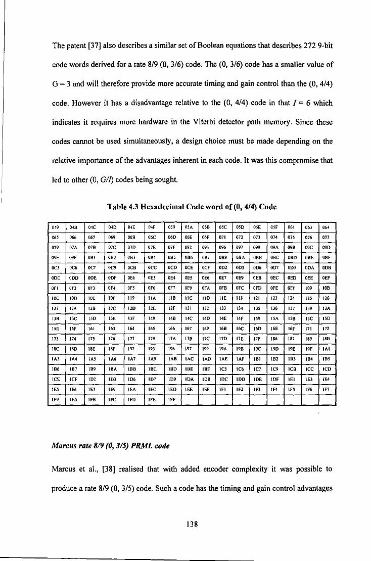
The patent [37] also describes a similar set ofBoolean equations that describes 272 9-bit

code words derived for a rate 8/9 (0, 3/6) code. The (0, 3/6) code has a smaller value of

G = 3 and will therefore provide more accurate timing and gain control than the (0, 4/4)

code. However it has a disadvantage relative to the (0, 4/4) code in that I = 6 which

indicates it requires more hardware in the Viterbi detector path memory. Since these

codes cannot be used simultaneously, a design choice must be made depending on the

relative importance of the advantages inherent in each code. It was this compromise that

led to other (0, G/1) codes being sought.

Table 4.3 Hexadecimal Code word of (0, 4/4) Code

0~9 O~B 04C 040 O~E O~F 059 05A 05B 05C 05D 05E 05F 061 061 OM

065 066 067 069 06B 06C 06D 06E 06F 071 072 073 074 075 076 077

079 07A 07B 07C OlD 07E 07F 092 09l 096 097 099 09A 09B 09C 09D

09E 09F OBI OB2 OBJ OB~ OB5 OB6 OB7 OB9 OBA OBB OBC OBD OBE OBF

00 OC6 OC7 OC9 OCB occ OCD OCE OCF OD2 ODJ OD6 OD7 009 ODA ODB

ODC ODD ODE ODF OEI OEJ OE4 OE5 OE6 OE7 OE9 OEB OEC OED OEE OEF

OFI OF2 OFl OF4 OF5 OF6 OF7 OF9 OFA OFB OFC OFD OFE OFF 109 lOB

IOC IOD IOE IOF 119 I lA IlB IIC IlD liE IIF 121 123 124 125 126

127 129 12B 12C 12D 12E 12F Ill ll2 133 134 135 136 Ill ll9 13A

llD llC 130 llE llF 149 14B 14C 14D 14E 14F IS9 ISA ISB ISC lSD

lSE ISF 161 163 164 16S 166 167 169 16B 16C 16D i6E 16F 171 172

173 174 17S 176 177 179 17A 17B 17C 17D 17E 17F 186 187 189 18B

18C lSD lSE 18F 192 193 196 197 199 19A 19B 19C 19D 19E 19F IAI

IA3 IA4 IAS IA6 IA7 IA9 lAB lAC lAD IAE IAF IBI IB2 IB3 184 IBS

186 187 189 IBA IBB IBC IBD IBE IBF IC3 IC6 IC7 IC9 ICB ICC ICD

ICE ICF ID2 IDl ID6 107 ID9 IDA IDB IDC IDD IDE IDF lE I I El IE4

IES IE6 IE7 IE9 lEA IEC lED lEE IEF IFI IF2 IF3 IF4 IFS IF6 IF7

IF9 IFA IFB IFC IFD IFE IFF

M arcus rate 819 (0, 3/5) PRML code

Marcus et al., [38] realised that with added encoder complexity it was possible to

produce a rate 8/9 (0, 3/5) code. Such a code has the timing and gain control advantages

138

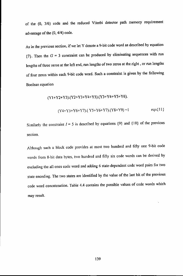
of the (0, 3/6) code and the reduced Viterbi detector path memory requirement

advantage of the (0, 4/4) code.

As in the previous section, if we let Y denote a 9-bit code word as described by equation

{7}. Then the G = 3 constraint can be produced by eliminating sequences with run

lengths of three zeros at the left end, run lengths of two zeros at the right , or run lengths

of four zeros within each 9-bit code word. Such a constraint is given by the following

Boolean equation

(Yl+Y2+Y3).(Y2+Y3+Y4+YS).(Y3+Y4+YS+Y6).

(Y4+Y5+Y6+Y7).( YS+Y6+Y7).(Y8+Y9) =l eqn{ll}

Similarly the constraint I = 5 is described by equations {9} and { l 0} of the previous

section.

Although such a block code provides at most two hundred and fifty one 9-bit code

words from 8-bit data bytes, two hundred and fifty six code words can be derived by

excluding the all-ones code word and adding 6 state-dependent code word pairs for two

state encoding. The two states are identified by the value of the last bit of the previous

code word concatenation. Table 4.4 contains the possible values of code words which

may result.

139

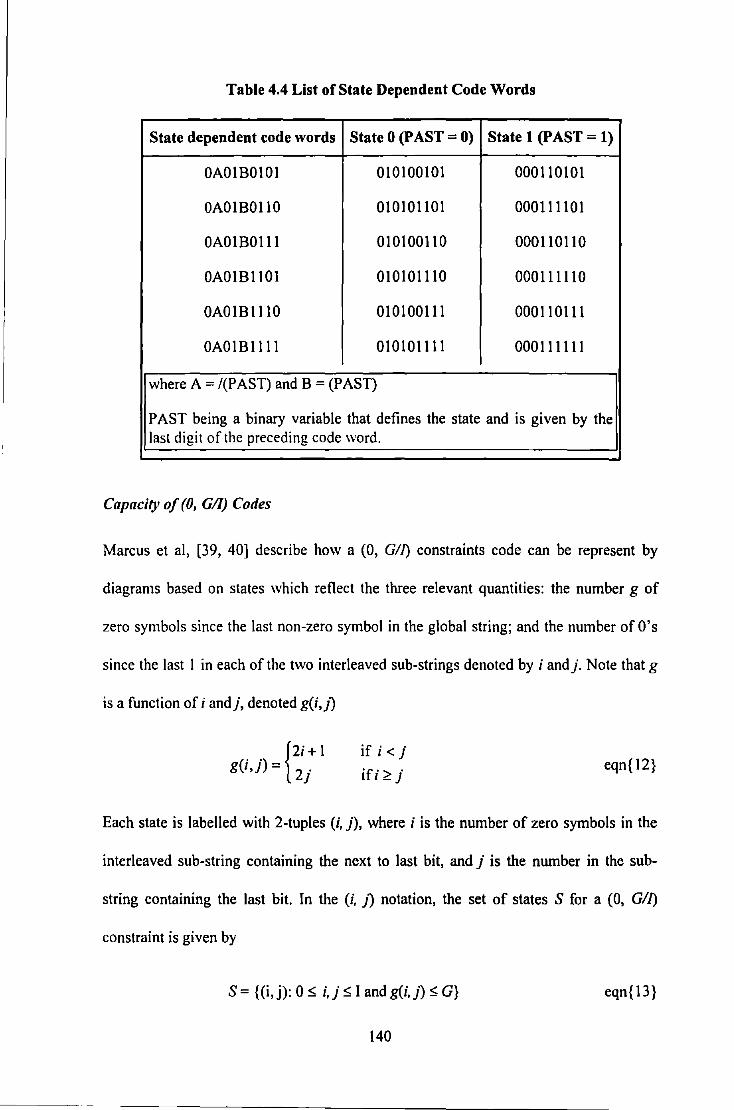
Table 4.4 List of State Dependent Code Words

State dependent code words State 0 (PAST = 0) State 1 (PAST= 1)

OAOIBOIOI 010100101 000110101

OAOIB0110 010101101 000111101

OA01B0111 010100110 000110110

OA01B1101 010101110 000111110

OAOIB1110 010100111 000110111

OA01B1111 010101111 000111111

where A = /(PAST) and B = (PAST)

PAST being a binary variable that defines the state and is given by the last digit of the preceding code word.

Capacity of (0, G/1) Codes

Marcus et al, [39, 40] describe how a (0, GII) constraints code can be represent by

diagrams based on states which reflect the three relevant quantities: the number g of

zero symbols since the last non-zero symbol in the global string; and the number of O's

since the last I in each of the two interleaved sub-strings denoted by i and j. Note that g

is a function of i and}, denoted g(i,J)

{2i +I

g(i,j) = 2j if i < j

ifi-:?.j eqn{12}

Each state is labelled with 2-tuples (i, j), where i is the number of zero symbols in the

interleaved sub-string containing the next to last bit, and j is the number in the sub-

string containing the last bit. In the (i, J) notation, the set of states S for a (0, GII)

constraint is given by

S = { (i, j): 0 ~ i, j ~I and g(i, J) ~ G} eqn{13}

140

and the transitions between states are given by the rules

"0" : (i, J) ~ (j, i+ I), provided (j, i+ I) e S

"1": (i,j) ~ (j, 0)

As an example consider the {0, 3/3) code. The state setS consists of the 12 states

{ (0, 0), (0, 1), {0, 2), {0, 3),

(1, 0), (1, 1), (1, 2), (1, 3),

(2, 0), (2, 1 ), {3, 0), (3, 1)}

The finite state transition matrix for this code is

(0,0) 0 0 0 0 0 0 0 0 0 0

(O,I) 0 0 0 0 I 0 0 0 0 0 0

(0,2) 0 0 0 0 0 0 0 0 I 0 0

(0,3) 0 0 0 0 0 0 0 0 0 0 I

(I,O) 0 0 0 0 0 0 0 0 0 0

(I, I) 0 0 0 0 I 0 I 0 0 0 0 0 B=

(1,2) 0 0 0 0 0 0 0 0 I 0 0 0

(1,3) 0 0 0 0 0 0 0 0 0 0 I 0

(2,0) 0 0 0 0 0 0 0 0 0 0

(2,I) 0 0 0 0 0 0 0 0 0 0

(3,0) I 0 0 0 0 0 0 0 0 0 0 0

(3,I) 0 0 0 0 0 0 0 0 0 0 0

The code capacity of the (0, 4/4) code can thus be calculated as the largest. real

Eigenvalue of the matrix. A brief summary of capacities and other parameters is given

in Table 4.5. For a more detailed table of capacities of(O, G/1) codes see [41).

141

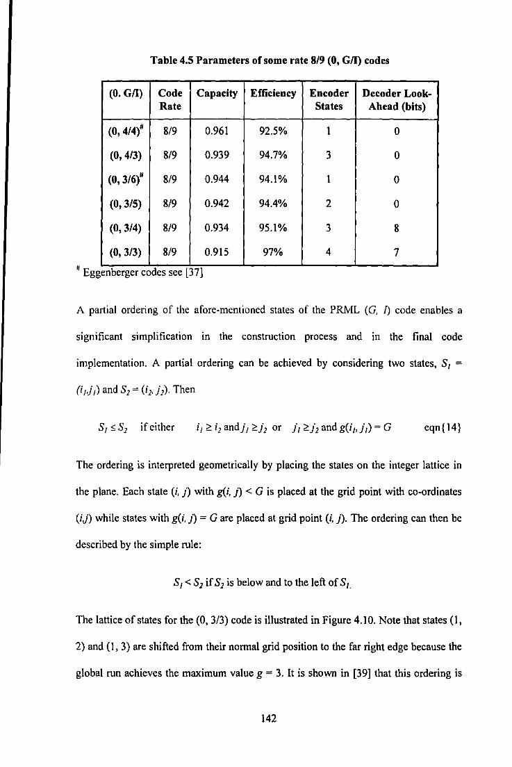
Table 4.5 Parameters of some rate 8/9 (0, G/1) codes

(0. G/1) Code Capacity Efficiency Encoder Decoder Look-Rate States Ahead (bits)

(0, 4/4)# 8/9 0.961 92.5% 1 0

(0, 4/3) 8/9 0.939 94.7% 3 0

(0, 3/6t 8/9 0.944 94.1% 1 0

(0, 3/5) 8/9 0.942 94.4% 2 0

(0, 3/4) 8/9 0.934 95.1% 3 8

(0, 3/3) 8/9 0.915 97% 4 7

# Eggenberger codes see [37]

A partial ordering of the afore-mentioned states of the PRML (G, I) code enables a

significant simplification in the construction process and in the final code

implementation. A partial ordering can be achieved by considering two states, S1 =

eqn{14}

The ordering is interpreted geometrically by placing the states on the integer lattice in

the plane. Each state (i, j) with g(i, j) < G is placed at the grid point with co-ordinates

(i,j) while states with g(i, J) = G are placed at grid point (i, j). The ordering can then be

described by the simple rule:

SI< s] if s2 is below and to the left of si.

The lattice of states for the (0, 3/3) code is illustrated in Figure 4.1 0. Note that states (1,

2) and (1, 3) are shifted from their nonnal grid position to the far right edge because the

global run achieves the maximum value g = 3. It is shown in [39] that this ordering is

142

the key to reducing the encoder complexity when designing codes using the state

splitting sliding block algorithm [42].

(0, 3). (1, 3).

(0, 2). (1,2).

(0, l). (1, l). (2, 1). (3, 1).

(0, 0). (1' 0). (2, 0). (3, 0).

Figure 4.10 Lattice of States for (0, 3/3) code

Finally, by applying an additional constraint, M, on the maximum run length of non-zero

samples, it has been shown in [43] that rate 8/9 codes remain viable at the expense of an

increased decoding window size. This result of adding the additional constraint can be

seen by comparing Table 4.5 with Table 4.6, for a modest increase in encoder/decoder

complexity an increase in code capacity can be realised.

Table 4.6 Properties of rate 8/9 (0, G/1) codes with M constraint

(0, G/1, M) Capacity Efficiency Encoder Encoder Look Decoder States Ahead (bits) Window (bits)

(0, 4/4, 9) 0.9603 92.56% 1 0 9

(0, 4/5, 6) 0.9624 92.36% 1 0 9

(0, 4/6, 5) 0.9587 92.71% 1 0 9

(0, 4/6, 4) 0.9437 94.19% 2 0 9

(0, 4/4, 5) 0.9457 93.98% 4 0 9

(0, 4/5, 4) 0.9395 94.6% 3 1 9

143

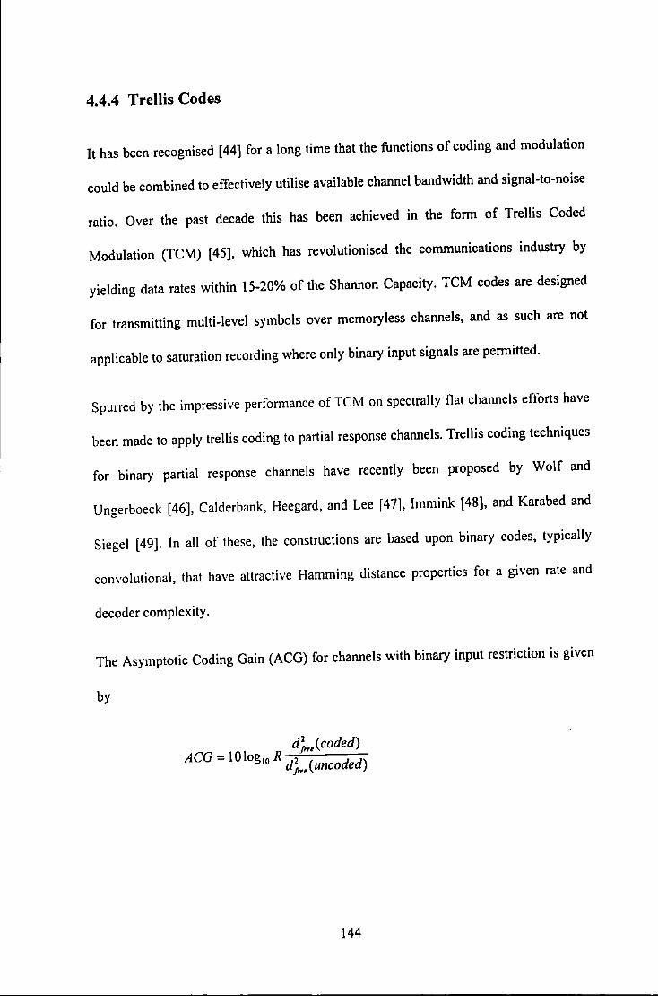
4.4.4 Trellis Codes

It has been recognised [44] for a long time that the functions of coding and modulation

could be combined to effectively utilise available channel bandwidth and signal-to-noise

ratio. Over the past decade this has been achieved in the form of Trellis Coded

Modulation (TCM) [45), which has revolutionised the communications industry by

yielding data rates within 15-20% of the Shannon Capacity. TCM codes are designed

for transmitting multi-level symbols over memoryless channels, and as such are not

applicable to saturation recording where only binary input signals are permitted.

Spurred by the impressive performance of TCM on spectrally flat channels efforts have

been made to apply trellis coding to partial response channels. Trellis coding techniques

for binary partial response channels have recently been proposed by Wolf and

Ungerboeck [46), Calderbank, Heegard, and Lee [47], Immink [48], and Karabed and

Siege! [49). In all of these, the constructions are based upon binary codes, typically

convolutional, that have attractive Hamming distance properties for a given rate and

decoder complexity.

The Asymptotic Coding Gain (ACG) for channels with binary input restriction is given

by

d],...(coded) ACG = 10log10 R d2 ( d d

1,.. unco e )

144

Trellis Coded Modulation

Ungerboeck [50] has proposed a channel coding technique that achieves coding gains

without sacrificing the data rate or expanding the bandwidth of the transmitted signal.

The basic idea is that by trellis coding onto an expanded modulation set (relative to that

needed for uncoded transmission) and by designing the trellis code to maximise the

minimum free Euclidean distance between allowable code sequences asymptotic (high

signal-to-noise ratio) coding gains of 3-6 dB compared to an uncoded system can be

achieved without bandwidth expansion. This is accomplished by encoding m

information bits, by means of a rate R =ml(m+ 1) convolutional encoder, into m+ I bits,

which select points from one of the conventional 2m+J signal constellations. The

mapping of information bits to coded bits is achieved by set partitioning.

The mapping ensures that the free Euclidean distance dfree between any two possible

sequences is greater than the minimum distance d0 between any two points in the 2m

signal constellation. Such memory can then be exploited by a maximum likelihood

decoder, yielding a coding gain of d1,e/ld/

The coding gain is a function of the amount of memory introduced by the encoder, i.e.,

the constraint length, and of the positioning of the signal points in the signal space, i.e.,

the signal constellation.

In summary, Ungerboeck's approach uses two key ideas:

a) In an uncoded system transmitting m bits of information in an interval T, one

of 2m signals are sent each T seconds. Ungerboeck has available 2m+1

signals

from which he chooses one every T seconds.

145

b) The rate R =ml(m+ 1) code limits the choice of signals to be transmitted. In

any key interval T only 2m of the 2m+/ are candidates for transmission. The set

partitioning rules specify which 2m signals are available at any instance in

time.

Wolf-Ungerboeck Rate 415 Trellis Code

Wolf and Ungerboeck [46] have described a coded system for improving the reliability

of digital transmission over a noisy partial-response channel with transfer function (1-

D). The (I-D) system uses a convolutional encoder that generates a binary convolutional

code with good free Hamming distance, followed by a precoder to increase the free

Euclidean distance between permitted channel output sequences. The addition of the

precoder causes the channel to resemble a spectrally flat channel. The maximum

likelihood decoder matched to the encoder, precoder and channel requires, in general,

2"+ 1 states where v is the constraint length of the convolutional encoder. Recently,

Zehavi and Wolf [51] showed that for a class of convolutional encoders the number of

states in the decoder is only 2" .

The rate 4/5 Wolf-Ungerboeck code can be described as having parameters {0, G/1) = (0,

44/22) and gives a coding gain of 3dB. Its trellis is shown in Figure 4.11 and the

associated path outputs are given in Table 4.7.

146

4 0 5 1 6 2 7 3

1115 10 14 9 13 8 12

12 8 13 9 14 10 15 11

2 6 3 7 0 4 1 5

1391281511141

5 1 4 0 7 3 6 2

10141115 812 913

21 1 7 20 16 23 19 22 18

26 30 27 31 24 28 25 29

18 22 19 23 1 6 20 17 21

29 25 28 24 31 27 30 26

19 23 18 22 1 7 21 1 6 20

28 24 29 25 30 26 31 27

20 16 21 17 22 18 23 1

27 31 26 30 25 29 24 28

Figure 4.11 Trellis for Rate 4/5 Wolf-Ungerboeck Code

147

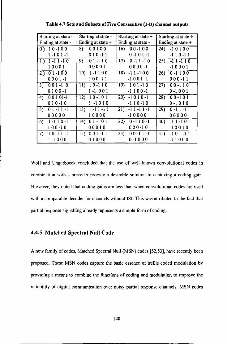
Table 4. 7 Sets and Subsets of Five Consecutive (1-D) channel outputs

Starting at state - Starting at state - Starting at state + Starting at state + Ending at state - Ending at state + Ending at state - Ending at state + 0) I 0-1 0 0 8) 00100 16) 0 0 -1 0 0 24) -10 I 00

1-101-1 0 1 0 -1 1 0-101-1 -110-11 1 ) 1-11-10 9) 0 1 -1 I 0 17) 0 -1 1 -1 0 25) -11-110

1 0 0 0 1 00001 0 0 0 0 -1 -1 0 0 0 1 2) 0 1 -1 0 0 10) 1 -1 I 0 0 18) -1 1 -1 0 0 26) 0 -1 1 0 0

0 0 0 I -1 1 0 0-1 1 -1001-1 0 0 0 -1 1 3) 0 0 I -1 0 11) 10-110 19) 1 0 1 -1 0 27) 0 0 -1 1 0

0 I 0 0-1 1 -1 0 0 1 -1100-1 0 -1 0 0 1 4) 00101-1 12) 1 0 -1 0 1 20) -1010-1 28) 0 0 -1 0 1

0 I 0 -1 0 1 -1 0 1 0 -110-10 0 -I 0 I 0 5) 01-11-1 13) 1-11-11 21) -11-11-1 29) 0-11-11

00000 10000 -1 0 0 0 0 00000 6) 1-110-1 14) 0 I -1 0 I 22) 0-110-1 30) -11-101

100-10 00010 000-10 -10010 7) 10-11-1 IS) 0 01-11 ?~) _.) 00-11-1 31) -101-11

1-1000 01000 0-1000 -I I 0 0 0

Wolf and Ungerboeck concluded that the use of well known convolutional codes in

combination with a precoder provide a desirable solution to achieving a coding gain.

However, they noted that coding gains are less than when convolutional codes are used

with a comparable decoder for channels without !SI. This was attributed to the fact that

partial response signalling already represents a simple form of coding.

4.4.5 Matched Spectral Null Code

A new family of codes, Matched Spectral Null (MSN) codes [52,53], have recently been

proposed. These MSN codes capture the basic essence of trellis coded modulation by

providing a means to combine the functions of coding and modulation to improve the

reliability of digital communication over noisy partial response channels. MSN codes

148

are constructed to have nulls • in the power spectrum precisely corresponding with those

of the channel transfer function. Class IV Partial Response channels have first order

nulls at zero frequency (d.c.) and at the Nyquist frequency. Unlike other trellis codes for

PR channels [46-49,], by matching these null frequencies, the MSN codes exploit, rather

than nullify, the inherent channel memory producing enhanced coding gains. Additional

coding gain is achieved by increasing the order of the spectral null of the code strings at

these frequencies.

The code described is designed for a (1-D) channel, but may be applied to a PR4

channel by interleaving, bit-wise, the code words. When interleaved the code satisfies

the constraints (0, G/1) = (0, I 0/5). The code is also designed to be 180 degrees phase­

shift invariant without requiring a precoder circuit. In other words the channel output

sequences a and -a both decode to the same data sequence b. The code is implemented

in a sliding block decoder that requires 4 states and one look-ahead code word.

Therefore the maximum length a single bit error from the detector can propagate is

limited to 2 bytes.

The full trellis for the matched spectral null code is quite complicated since a rate 8/10

code has i=256 branches leaving every state. Thus an alternative to true maximum

likelihood decoding was achieved by using a trellis structure derived from the spectral

null diagram, illustrated in Figure 4.12, that has a maximum DSV=6. The code words of

the rate 8/10 MSN code are a subset of the code words of a slightly larger code which

has a much simpler trellis. However, for any MSN code word, no word in the larger

' Those frequencies at which the power spectrum value is zero, due to no energy transmission.

149

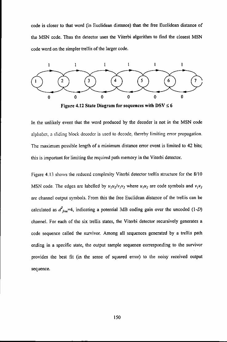
code is closer to that word (in Euclidean distance) than the free Euclidean distance of

the MSN code. Thus the detector uses the Viterbi algorithm to find the closest MSN

code word on the simpler trellis of the larger code.

0 0 0 0 0 0

Figure 4.12 State Diagram for sequences with DSV ~ 6

In the unlikely event that the word produced by the decoder is not in the MSN code

alphabet, a sliding block decoder is used to decode, thereby limiting error propagation.

The maximum possible length of a minimum distance error event is limited to 42 bits;

this is important for limiting the required path memory in the Viterbi detector.

Figure 4.13 shows the reduced complexity Viterbi detector trellis structure for the 8/10

MSN code. The edges are labelled by u1r1/v1v2 where u1u2 are code symbols and v1v2

are channel output symbols. From this the free Euclidean distance of the trellis can be

calculated as ~1, •• =4, indicating a potential 3dB coding gain over the uncoded (1-D)

channel. For each of the six trellis states, the Viterbi detector recursively generates a

code sequence called the survivor. Among all sequences generated by a trellis path

ending in a specific state, the output sample sequence corresponding to the survivor

provides the best fit (in the sense of squared error) to the noisy received output

sequence.

150

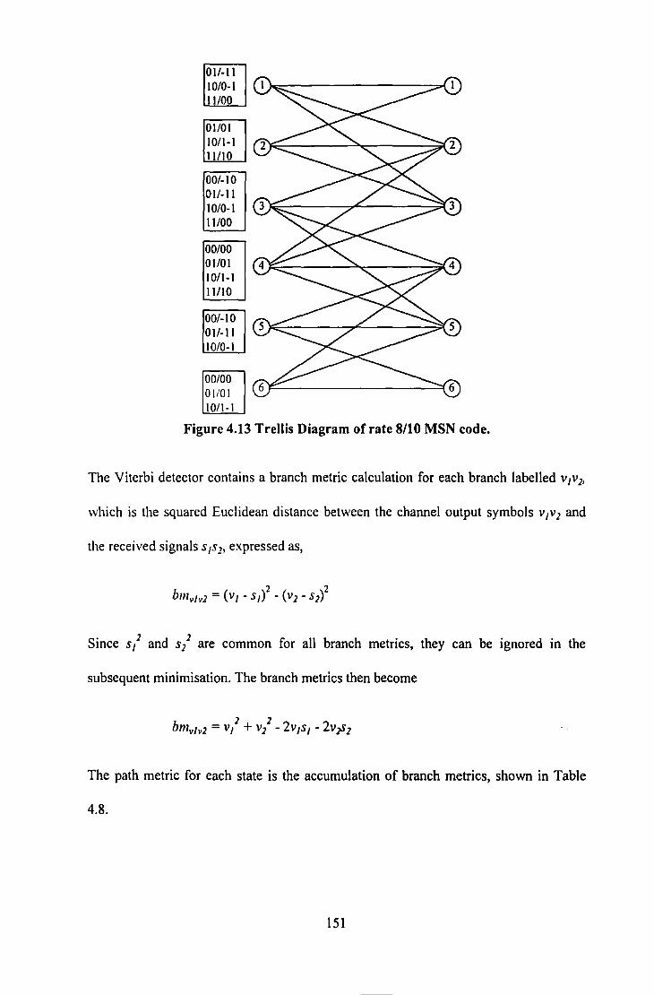
011-11 10/0-1 11/00

01/01 10/1-1 I Ill 0

00/-10 01/-11 10/0-1 11/00

00/00 01/01 10/1-1 11/10

00/-10 01/-11 10/0-1

00/00 01/0 I 10/1-1

Figure 4.13 Trellis Diagram of rate 8/10 MSN code.

The Viterbi detector contains a branch metric calculation for each branch labelled v1v2,

which is the squared Euclidean distance between the channel output symbols v1v2 and

the received signals s 1sb expressed as,

Since s/ and s/ are common for all branch metrics, they can be ignored in the

subsequent minimisation. The branch metrics then become

The path metric for each state is the accumulation of branch metrics, shown in Table

4.8.

151

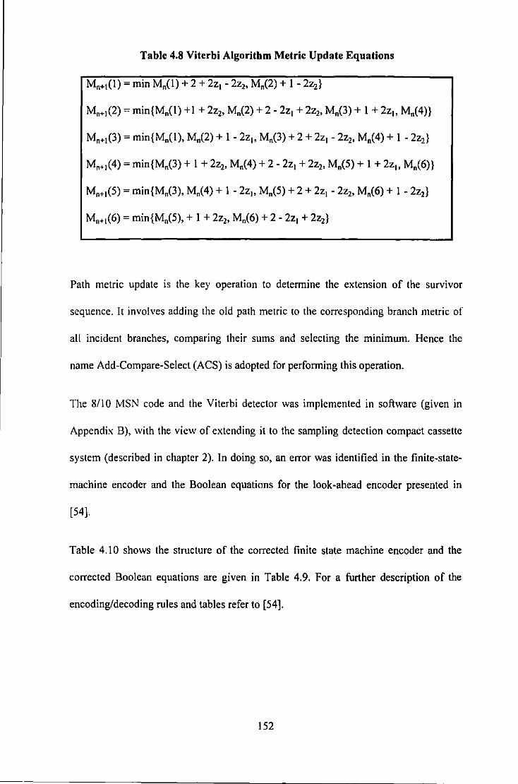
Table 4.8 Viterbi Algorithm Metric Update Equations

Mn+t{l) = min M0{1) + 2 + 2z,- 2z2, M0 (2) + I - 2z2}

Mn+1(2) = min{M0(1) +I+ 2z2, M0(2) + 2- 2z1 + 2z2, M0(3) +I+ 2z~o M0 (4)}

Mn+1(3) = min{M0{1), M0 (2) + I - 2zl> M0 (3) + 2 + 2z,- 2z2, M0 (4) +I - 2z2}

M0 +1(4) = min{M0 (3) + I + 2z2, M0 (4) + 2- 2zt + 2z2, M0(5) +I + 2zl> M0 (6)}

Mn+1(5) = min{M0(3), M0(4) +I - 2zt> M0 (5) + 2 + 2zt- 2z2, M0 (6) + I - 2z2}

Mn+ 1(6) = min{M0(5), + I + 2z2, M0(6) + 2- 2z1 + 2q}

Path metric update is the key operation to determine the extension of the survivor

sequence. It involves adding the old path metric to the corresponding branch metric of

all incident branches, comparing their sums and selecting the minimum. Hence the

name Add-Compare-Select (ACS) is adopted for performing this operation.

The 8110 MSN code and the Viterbi detector was implemented in software (given in

Appendix B), with the view of extending it to the sampling detection compact cassette

system (described in chapter 2). In doing so, an error was identified in the finite-state­

machine encoder and the Boolean equations for the look-ahead encoder presented in

[54].

Table 4.I 0 shows the structure of the corrected finite state machine encoder and the

corrected Boolean equations are given in Table 4.9. For a further description of the

encoding/decoding rules and tables refer to [54].

!52

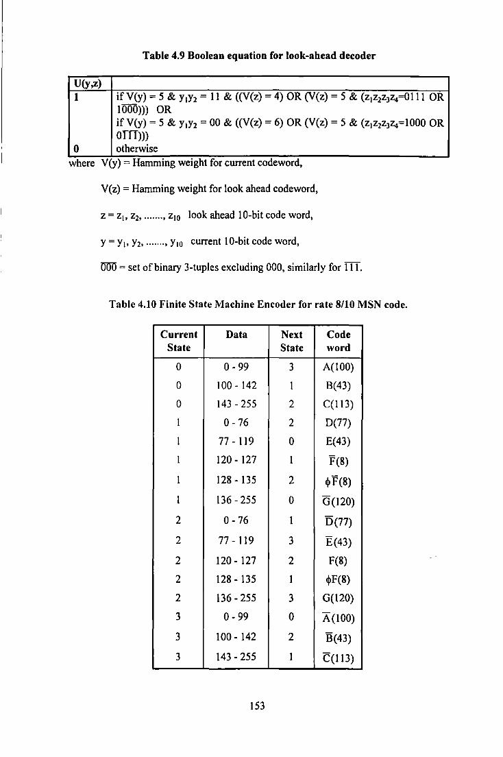
Table 4.9 Boolean equation for look-ahead decoder

U(y,z) 1 ifV(y)- 5 & y1y2 - 11 & ((V(z)- 4) OR (V(z)- 5 & (z1 z2z3~-0IIJ OR

1000))) OR if V(y) = 5 & y1y2 = 00 & ((V(z) = 6) OR (V(z) = 5 & (z1 z2z3~=1000 OR Offi)))

0 otherwise where V(y) = Hammmg we1ght for current codeword,

V(z) =Hamming weight for look ahead codeword,

z = zl> z2, ••••••• , z10 look ahead I O-bit code word,

Y = Y1• Y2 • ....... , y10 current 10-bit code word,

mm= set of binary 3-tuples excluding 000, similarly for m.

Table 4.10 Finite State Machine Encoder for rate 8/10 MSN code.

Current Data Next Code State State word

0 0-99 3 A(100)

0 100-142 I B(43)

0 143- 255 2 C(113)

I 0-76 2 D(77)

I 77-119 0 E(43)

I 120- 127 I F(8)

I 128-135 2 ~F(8)

I 136-255 0 0(120)

2 0-76 I D(77)

2 77-119 3 E(43)

2 120- 127 2 F(8)

2 128- 135 1 ~F(8)

2 136- 255 3 0(120)

3 0-99 0 A(IOO)

3 100- 142 2 B(43)

3 143- 255 1 C(113)

153

lio 'implement: ~this code• oil the sampling ;compact CaSSette s}'stem W()!i)di require:

. . '

.a,!iditional•equalisatlonlto optiinise the channeli response _:to that ofPR4;, a<s~:parate clock

re~()very circuit and1 a more powerful processor, to implement.the real~time computation

required by .the Viterbi A:lgorith.m. 'Therefore this code was m>t· successfully appliedi to

tbe leXperimentai recotcling; system. However; it w~ implemented,. in Pascal1, ·Using

simula:ted' Loreritziart .pulses, H .wou)dl be \in fair to c;ompare the 'simulated! results against

,those obtaine'd from prf!ctical experimentation sine(! realistic noise1models haye:riot been•

developed.

:154

4.4.6 Coding for EPR4 Channels

The choice of class IV partial response is not a good match to very high density

magnetic recording channels or to channels using minimum runlength constraints. In

such cases, higher order PR polynomials must be used, leading to exponential growth in

the complexity of the Viterbi detector.

(1, 7)ML Code

Pate! (55,56] has recently proposed a detection scheme for channels with a minimum

run-length constraint of (d =I) two bit intervals between transitions. Instead of

equalising the channel to a PR4 response, the channel is equalised to an enhanced class

IV partial response transfer function (I + D - d - D\ This scheme achieves near

maximum likelihood performance without Viterbi computations by addressing only the

most likely error events. This leads to a detector which requires 1 5 adders and a

relatively simple finite state machine. However, the optimality of the equaliser extends

only over a limited range of densities.

By employing a d=l constrained code the density ratio on the magnetic medium is

improved by a factor of 1.5, from 8/9 in conventional PRML channels to 4/3 in the new

channel. It also controls the !SI and increases decoding reliability by removing many

error prone paths from the trellis.

The trellis diagram for an EPR4 channel sequence, as shown in Figure 4.14a, has eight

states. By applying (1,7) code constraints two states, (010), (101), are eliminated, and a

further two, (00 I), (11 0), become transitional only resulting in the trellis illustrated in

155

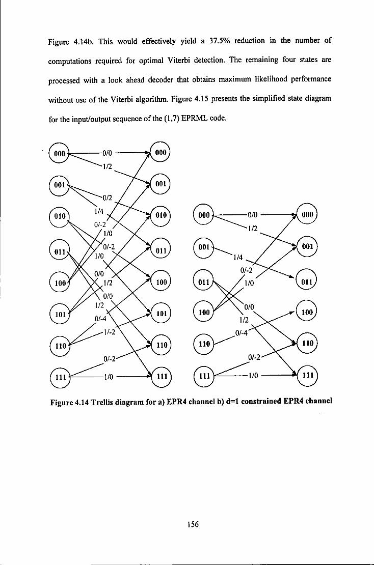
Figure 4.14b. This would effectively yield a 37.5% reduction in the number of

computations required for optimal Viterbi detection. The remaining four states are

processed with a look ahead decoder that obtains maximum likelihood performance

without use of the Viterbi algorithm. Figure 4.15 presents the simplified state diagram

for the input/output sequence of the (1,7) EPRML code.

~0/0 -------.1

1/2

0/-2

~1/0 ------<-"'!

~0/0----..1 1/2

~ ~1/4

0/-2

~0/-4

0/-2

~1/0 ------<ill/

Figure 4.14 Trellis diagram for a) EPR4 channel b) d=l constrained EPR4 channel

156

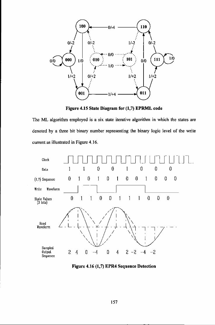
0/-2 0/-2 11-2 0/-2 . . ·~.. 0/0 ,.; •·• -""'!~··· --·--·.·· ....

110 ~ 010 ; : 101 ; 0/0 · .. 4 .. -·: ... 110 ............. ·· . . . . . .

11+2 0/+2 1/+2 11+2

Figure 4.15 State Diagram for (1,7) EPRML code

The ML algorithm employed is a six state iterative algorithm in which the states are

denoted by a three bit binary number representing the binary logic level of the write

current as illustrated in Figure 4.1 6.

Clock JLn_llfl Dala 1 0 0 0 0 0

( 1,7) Sequence 0 1 0 0 0 0 1 0 0 0

Wrilc Waveform

Slale Values (3 bils)

Read Waveform

Sampled Oulpul Sequence

0 1

_L_~_

\ \

' ' '~ 2 4 0 -~

0 0 0 0 0

0 4 2 -2 -4 -2

Figure 4.16 (1,7) EPR4 Sequence Detection

!57

The states (100), (000), and (001) correspond to the detection of a positive read pulse

and possess mirror image symmetry (+/- sign) with states (011), (111), and (110)

respectively that correspond to the negative pulse.

The detector is state dependent and requires a look ahead of five samples, i.e. given the

current state aob0c0 and the sample values y0 , Y~o y2, y3, and y4, the detector determines

the noise free sample value y0, and the resultant next state a1b1c1 • More recently the

detector has been increased to a six sample look ahead to reduce errors caused by certain

dibit combinations at high density [59]

The detector makes its decision on the outcome of three basic checks, namely:

a) the baseline check,

b) the peak-position check,

c) the phase check.

Each check is a comparison of a specific function of the sampled values against a fixed

threshold, and is represented by a Boolean variable. Each threshold is represented by a

corresponding constant that is strongly related to the shape of the readback signal. The

linear functions and their thresholds are chosen so as to minimise the overall mean

squared error in the sequence detection process. Table 4.11 lists these functions with the

decision boundaries and the functions are classified in accordance with their functional

role in the detection process. Table 4.12 shows the ML state decoder driven by the

decision function AB+ X+ YZ and phase check p.

158

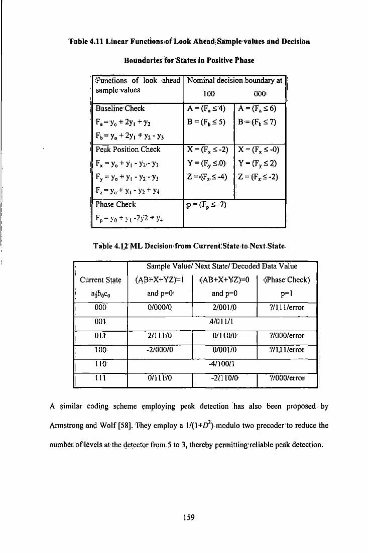
'Fable 4.11 Linear Fum':tions,ofLook A:heild!Silinple·valiJ~s and Decision

Bm.md~tries for'State!i in Positive Phase

'Functions of look ahead Nominal' decision boundary at ' I sample values 100 0001

' I

i BaseJine;Ch~ck A- (F.~4)

I A= (F.~ 6)

' 'F.=yo+2yl +y2 B = (Fb ~ 5) .B:=(Fb ~ 7) I

h=yo+2yi+Y2-YJ I i I Peak Position 8heck X =(F.~ -2) X= (F.~ -0)

I

I F.= Yo + Y1 "Y2:-YJ y = (F:y ~.0); I

y == (Fy ~ 4) I

fy = Yo + Y1 -yr-YJ Z =1(Fz ~;-4) i · Z = (Fz ~ -2)

F z = Yo + Y,l , Y2 + Y4 I

': I Phase Check p-(Fp~-7) ' ' ' Fr= Yo + Y1 -2y2 + Y4 ' '

I I

Table 4.J2' ML Decision• from Current:State ,to Next State.

Sample Value/ Next State/' Decoded !Data Value i

Current St(lte (AB+X+YZ)=I {AB+X+Y:Z)=O Whase Check)

I aoboco and'p=O· andp='O p=l

I 000 0/000/0 2/00110 ?/1.1 1/error

001 4101111 !

! 01!1' 2/,Jll'/0 0/I;I 0/0 ?/000/error

'

' lOO -2/000/0 0/001/0 ?IU 1/error '

I

I 110 A/100/1 '

'

I 1H OJ.l 1HO -2/ll0/0· ?/000/error

I

A similar codipg scheme employing peak detection has also been proposed ·by

Aimstrong ,ang1 Wolf [58], lihey employ a 1'/(1 +d) modulo two precoder'to reduce the

Ji.umber of1levels atthe cietector from.S to 3, thereby permitting• reliable peak detection;

159

4.5 Discussion

Analytical studies have shown that PRML can potentially increase the recording density

by 80-100% when compared to MFM recording [59), and by 30-50% when compared to

RLL {1,7) or {2,7) coding [59,33].

Several codes applicable to a digital magnetic recording channel employing partial

response signalling and maximum likelihood detection have been presented.

The Eggenberger 8/9 (0, 4/4) codes have been adopted by hard disk drives due to their

high code rate and their ability to simplify the Viterbi detector for class IV partial

signals.

More advanced trellis codes have been proposed by Wolf and Ungerboeck that yield

approximately 3d8 advantage over baseline class IV partial response at the expense of a

reduction in code rate and a dramatically increased complexity Viterbi detector. The

matched spectral null code goes some way to alleviating the problem of the complexity

of the Viterbi detector as well as matching the spectral properties of the channel.

The theory of MSN codes is appealing from the intuitive standpoint. It is consistent with

the well known adage that "the code spectrum should match the channel transfer

characteristics". A recent paper [60) comparing the rate 8/9 {0, 4/4) code against the· rate

8/1 0 MSN code for an experimental hard disk system has shown that the 8/10 MSN

code reduces the "On-track Error Rate" by at least 2 orders of magnitude and gives a 10-

20% increase in "Off-track Capability" at bit error rate of 10-6. The overall improvement

160

in linear density is in excess of 17% which, when combined with superior track pitch

requirements yields approximately 20% increase in the area) density.

Higher orders of partial response schemes have also been proposed that would require a

greater complexity Viterbi detector. The RLL 2/3 (1,7) code has been proposed to

simplify the Viterbi detection for the EPR4 channel. Employing this code would result

in a code rate loss with respect to other codes described. However, this is balanced by

reduced loss through the equaliser, due to the fact that EPR4 is a better match than PR4

to the magnetic recording channel at higher densities. Another advantage of this code is

that at high linear densities non-linear errors occur due to the medium not being able to

support such closely spaced transition. Hence, by employing a d= I constrained code the

transitions are further apart therefore permitting greater capacity.

Attempts made to employ 8/10 MSN on the compact cassette magnetic recording

system high-lighted the fact that a great deal of signal processing power is required for

successful PRML systems, for maximum-likelihood detection, and for equalisation, as

well as the coding. Therefore more efficient codes are sometime rejected in favour of

those that simplify the detection process. Hence, commercial disk drive applications

have chosen to go with 8/9 (0, 4/4) code. However, as processing power becomes more

widely available and less costly other more efficient coding schemes may be adopted.

161

4.6 References

1. Fomey, Jr., G.D., "Maximum-Likelihood Sequence Estimation of Digital

Sequence in the presence of lntersymbol Interference", IEEE Trans. Inf. Theory,

Vol.l8, No.3, pp.363-78, May 1972.

2. Viterbi, A.J., "Error Bounds for Convolutional Codes and an Asymptotically

Optimum Decoding Algorithm", IEEE Trans. Inf. Theory, Vol.l3, No.2, pp.260-

69, April 1967.

3. Omura, J.K., "On The Viterbi Decoding Algorithm", IEEE Trans. on Inf. Theory,

Vo1.15, pp.177-79, January 1969.

4. Fomey, Jr., G.D., 'The Viterbi Algorithm", Proc. IEEE, Vol.61, pp.268-278,

March 1973.

5. Haynes, J.F., "The Viterbi Algorithm Applied to Digital Data Transmission",

IEEE Comm. Soc. Mag., Vol.l3, No.2, pp.l5-20, March 1975.

6. Kobayashi, H., "Application of Probalistic Decoding to Digital Magnetic

Recording Systems", IBM J. Res. Develop., pp.64-74, January 1971.

7. Nakagawa, S., et al., "A Study on Detection Methods of NRZ Recording", IEEE

Trans. Magn., Vol.MAG-16, No.!, pp.l04-10, January 1980.

8. Dolivo, F., Hermann, R., & Olcer, S., "Performance & Sensitivity Analysis of

Maximum-Likelihood Sequence Detection on Magnetic Recording Channels",

IEEE Trans. Magn., Vol.25, No.5, pp.l399-1401, September 1989.

9. Moon, J.J., & Carely, L.R., "Performance Comparisons of Detection Methods in

Magnetic Recording", IEEE Trans. Magn., Vol.26, No.6, pp.3155-72, November

1990.

162

10. Cioffi, J.M., & Melas, C., "Evaluating the Perfonnance of Maximum Likelihood

Sequence Detection in a Magnetic Recording Channel", Globecom '86 (Houston,

Texas), pp.l 066- 70, December 1986.

11. French, C.A., & Wolf, J.K., "Application of the Viterbi Algorithm to the

Detection of Compact Spectrum", IEEE Trans. Magn., Voi.MAG-22, No.S,

pp.l200-1202, September 1986.

12. Schneider, R.C., "Sequence (Viterbi-Equivalent) Decoding", IEEE Trans. Magn.,

Vol.24, No.6, pp.2539-41, November 1988.

13. Shafiee, H., & Moon, J., "Low Complexity Viterbi Detection for a Family of

Partial Response Systems", IEEE Trans. Magn., Vol.28, No.S, pp.2892-94,

September 1992.

14. Wood, R., "Turbo-PRML: A Compromise EPRML Detector", IEEE Trans.

Magn., Vol.29, No.6, pp.4018-20, November 1993.

15. Fano, R.M., "A Heuristic Discussion of Probabilistic Decoding", IEEE Trans. Inf.

Theory, Vol.9, pp.64-74, April 1963.

16. Nyquist, H., "Certain Topics in Telegraph Transmission Theory", Transactions of

the American Institute of Electrical Engineers, pp.617-44, April 1928.

17. Lender, A., "The Duo-Binary Technique for High Speed Data Transmission",

IEEE Trans. on Comm. & Electronics, Vol.83, pp.214-18, May 1963.

18. Lender, A., "Faster Digital Communications with Duo-Binary Techniques",

Electronics, Vol.22, pp.61-65, March 1963.

19. Kretzmer, E.R., "Generalization of a Technique for Binary Data Communication",

IEEE Trans. Comms. Tech. (Concise Papers), Voi.COM-14, pp.67-68, February

1968.

163

20. Kabel, P., & Pasupathy, S., "Partial Response Signaling", IEEE Trans. Comm.,

Vol.COM-23, No.9, pp.921-934, September 1975.

21. Kobayashi, H., & Tang, D.T., "Application of Partial Response Channel Coding

to Magnetic Recording Systems", IBM J. Res. Develop., Vol.l4, pp.368-375, July

1970.

22. Thapar, H.K., & Pate!, A. M., "A Class of Partial Response System for Increasing

Storage Density in Magnetic Recording", IEEE Trans. Magn., Vol.23, No.5,

pp.3666-68, September 1987.

23. Lender, A., "Correlative Digital Communication Techniques", IEEE Trans.

Comm. Tech., Vol.COM-12, pp.l28-35, 1964.

24. Coleman, C.H., Lindholm, D.A., Petersen, D.A., & Wood, R., "High Data Rate

Magnetic Recording in a Single Channel", J.IERE Vo1.55, No.6, pp.229-236, June

1985.

25. Wood, R. W., & Petersen, D.A., "Viterbi Detection of Class IV Partial Response

on a Magnetic Recording Channel", IEEE Trans. Comms., Vol.34, No.5, pp.454-

461, May 1986.

26. Watkinson, J.R., "The Technology of the Ampex DCRSi", IERE 7th Int. Conf.

Video, Audio & Data Recording, pp.l59-65, March 1988.

27. Russ, K., "Digital Tape Transport for Military Data", Electronic Product Design,

pp.37-40, August 1989.

28. Wood, T.G., "A Survey of DCRSi and D-2 Technology", IEEE lOth Symp. on

Mass Storage Systems - Digest of Papers, pp.46-50, 1990.

164

29. Bergmans, J.W.M., Mita, S., Izumita, M., & Doi, N., " Partial- Response

Decoding of Rate l/2 Modulation Codes for Digital Storage", IEEE Trans.

Comms., Vol.39, No.11, pp.1569-81, November 1991.

30. Bergmans, J.W.M., "A Partial-Response Receiver for Miller- Squared Encoded

Signals with Half the Usual Operating Speed", IEEE Trans. Magn., Vol.26, No.5,

pp.2925-30, September 1990.

31. Wood, R.W., "Viterbi Detection of Miller-squared code on a tape channel", IERE

4th Int. Conf. on Video & Data Recording, Proc.54, Southampton, England,

pp.333-334, April 20-23 1982.

32. Ferguson, M.J., "Optimal Reception for Binary Partial Response Channels", Bell

System Tech. Journal, Vol.51, No.2, pp.493-505, February 1972.

33. Dolivo, F., Ungerboeck, G., & Howell, T.D., "Decoding the Output Signal of a

Partial-Response Class-IV Communication or Recording-Device Channel.", U.S.

Patent 4,644,564., 17 Febuary. 1987.

34. Howell, T.D., McCrown, D.P., Diola, T.D., Tang, Y., Hense, K.R., & Gee, R.L.,

"Error Rate Performance of Experimental Gigabit per Square Inch Recording

Components", IEEE Trans Magn., Vo1.26, No.5, pp.2298-302, September 1990.

35. Coker, J.D., Galbraith, R.L., Kerwin, G.J., Rea, J.W., & Ziperovich, P.A.,

"Integrating a Partial Response Maximum Likelihood Data Channel into the IBM

0681 Disk Drive", Proceedings of the 24th Asilomar Conf. (Monterey), pp.674-

677, November 1990.

36. Coker, J.D., Galbraith, R.L., Kerwin, G.J., Rea, J.W., & Ziperovich, P.A.,

"Implementation of PRML in a Rigid Disk Drive", IEEE Trans. Magn., Vol.27,

No.6, pp.4538-43, November 1991.

165

37. Eggenberger, J.S., & Pate!, AM., "Method and Apparatus for Implementing

Optimum PRML Codes", U.S. Patent 4,707,681., 17 November 1987.

38. Marcus, B.H., Pate!, AM., & Siege!, P.H., "Method and Apparatus for

Implementing a PRML Code", U.S. Patent 4,786,890., 22 November 1988.

39. Marcus, B.H., & Siege!, P.H., "Constrained Codes for PRML", IBM Research

Report, RJ 4371 (47629}, 31 July 1984.

40, Marcus, B.H., Siege!, P.H., & Wolf, J.K., "Finite-State Modulation Codes for

Data Storage", IEEE J. Select. Areas Comms., Vol.IO, No.!, pp.S-37, January

1992.

41. Stefanovic, M.C., & Vasic, B. V., "Channel Capacity of (O,G/1) Code", Electronic

Letters, Vol.29, No.2, pp.243-45, January 1993.

42. Karabed, R., & Marc\ls, B.H., "Sliding Block Coding for Input Restricted

Channels;', IEEE Trans. Irtf. Theory, Vol.34, No. I, pp.2-26, January 1988.

43. Cideciyan, R.D., Dolivo; F., Hermann, R., Hirt, W., & Schott, W., "A PRML

System for Digital Magnetic Recording", IEEE J. Se!. Areas in Comms.; Vol.lO,

No.1, pp.38-56, January 1992.

44. Shannon, C.E., "A Mathematical Theory of Communications", Bell Syst. Tech.

Journal, Vol.27, No.J, pp.379-423:623-656, July 1948.

45. Ungerboeck, G., "Trellis-Coded Modulation with Redundant Signal Sets", IEEE

Comms. Mag., Vol.25, No.2, pp.S-21, February 1987.

46. Wolf, J.K., & Ungerboeck, G., "Trellis Coding for Partial Response Channels",

IEEE Trans. Comms., Vol.34, No.8, pp.765-73, August 1986.

166

47. Calderbank, A.R., Heegard, C., & Lee, T.A., "Binary Convolutional Codes with

Applications to Magnetic Recording", IEEE Trans. Inf. Theory, Vol.32, No.6,

pp.797-815, November 1986.

48. Immink, K.A.S., "Coding Techniques for the Noisy Magnetic Recording Channel:

A State-of-the-Art Report", IEEE Trans. Comms., Vol.37, pp.413-419, May 1989.

49. Karabed, R., & Siege!, P.H., "Trellis Codes for Partial Response Channels", U.S.

Patent 4,888,775., 19 December 1989.

50. Ungerboeck, G., "Channel Coding with Multilevel/Phase Signals", IEEE Trans.

In f. Theory, Vo1.28, No.l, January 1982.

51. Zehavi, E., & Wolf, J.K., "On Saving Decoder States for Some Trellis Codes and

Partial Response Channels", IEEE Trans. Comms., Vol.36, No.2, pp.222-224,

February 1988.

52. Karabed, R., & Seigel, P.H., "Matched Spectral Null Trellis Codes for Partial

Response Channels", U.S. Patent 4,888,779., March 1988.

53. Karabed, R., Seigel, P.H., "Matched Spectral Null Codes for Partial Response

Channels", IEEE Trans. Inf. Theory, Vol.37, No.3, pp.818-54, May 1991.

54. Thapar, H.K., et al., "On the Perfonnance of a Rate 8/10 Matched Spectral Null

Code for Class-4 Partial Response", IEEE Trans. Magn., Vol. 28, No.5, pp.2883-

88, September 1992.

55. Pate!, A.M., "Method & Apparatus for Processing Sample Values in a Coded

Signal Processing Channel", U.S. Patent 4,945,538., 31 July 1990.

56. Pate!, A.M., "A New Digital Signal Processing Channel for Data Storage

Products", IEEE Trans. Magn., Vol.27, No.6, pp.4579-84, November 1991.

167

57. Dolivo, F., Maiwald, D., & Ungerboeck, G., "Partial-Response Class IV

Signalling with Viterbi Decoding Versus Conventional Modified Frequency

Modulation (MFM) in Magnetic Recording", IBM Research Report RZ 973, 23rd

July 1979.

58. Annstrong, A.J., & Wolf, J.K., "Coded Partial Response Signalling with Peak

Detection", IEEE Global Telecommunications Conf. (Globecom '90), pp.l782-86,

1990.

59. Thapar, H.K., and Howell, T.D., "On the perfonnance of Partial Response

Maximum-Likelihood and Peak Detection methods in Magnetic Recording",

Tech. Dig. Magn. Rec. Conf., Hidden Valley, PA, June 1991.

60. Thapar, H.K., Shung, C.B., Rae, J.W., Karabed, R., & Seigel, P.H., "Real Time

Recording Results for a Trellis Coded Partial Response (TCPR) System", IEEE

Trans. Magn., Vo1.29, No.6, pp.4009-ll, November 1993.

168

CHAPTERS

Two Dimensional (Multi-Track) Coding

5.1 Introduction

This chapter describes a new class of modulation codes that exploits the two­

dimensional properties of a multi-track digital magnetic recording systems. Marcellin &

Weber [I] first recognised that Two Dimensional or Multi-track Modulation codes, as

they are known, provide the capacity to substantially increase data storage density by

operating on several tracks in parallel. Their paper demonstrates how the run-length, of

a recording code, could be shared over several channels in a multi-channel environment

by relaxing the k constraint along each individual track whilst maintaining a common ky

constraint across the tracks. Since multiple tracks are read out in parallel, it is not

necessary for each individual track to provide all the clocking information required to

maintain clock synchronisation. Instead, the clocking information derived from frequent

transitions and defined by the k constraint, can now be sub-divided over several tracks

giving a ky constraint. By allowing the Js, constraint to be met across the tracks many

more code words are possible for a given d, and Js, in two dimensions than was possible

in one dimension.

169

Swanson & Wolf [2] noted that the prime disadvantage of the proposed codes was their

vulnerability to the loss of a channel due to poor clock recovery. In magnetic tape

recording the loss of a channel for long periods of time is not uncommon due to

problems such as head clog or medium dropouts. Therefore, in the event of a burst error

on a particular track containing the majority of timing information (transitions), the

result would be fatal since the clock recovery would not function correctly causing mis­

synchronisation. They noted for practical implementation, it is essential to distribute the

timing information equally across all channels, so that in a single-track error situation,

clock recovery is maintained by transitions from other tracks. To address this problem

they proposed the addition of a kx constraint, to impose a maximum run-length along

each track without a transition, assuring sufficient timing information even if one

channel is completely lost.

This type of coding scheme is thus characterised by (d, k"' ky; y). Where the d constraint

must be satisfied for each track independently to avoid inter-symbol interference, kx, ky

are the k constraints satisfied along, and across they number of tracks respectively. The

inclusion of the cross channel constraint ky allows the kx constraint to be much larger

than the customary k so that capacity can be increased over conventional, single

channel, RLL codes.

Finally, this chapter will describe the author's work in designing a two-dimensional

coding scheme for the multi-track compact cassette system described in chapter 3.

Further, the development of a multi-dimensional coding scheme for a high density,

multi-track system that employs partial response and maximum likelihood detection

along the tracks is described. A discussion on how error correction could also be

incorporated into two-dimensional codes is also presented.

170

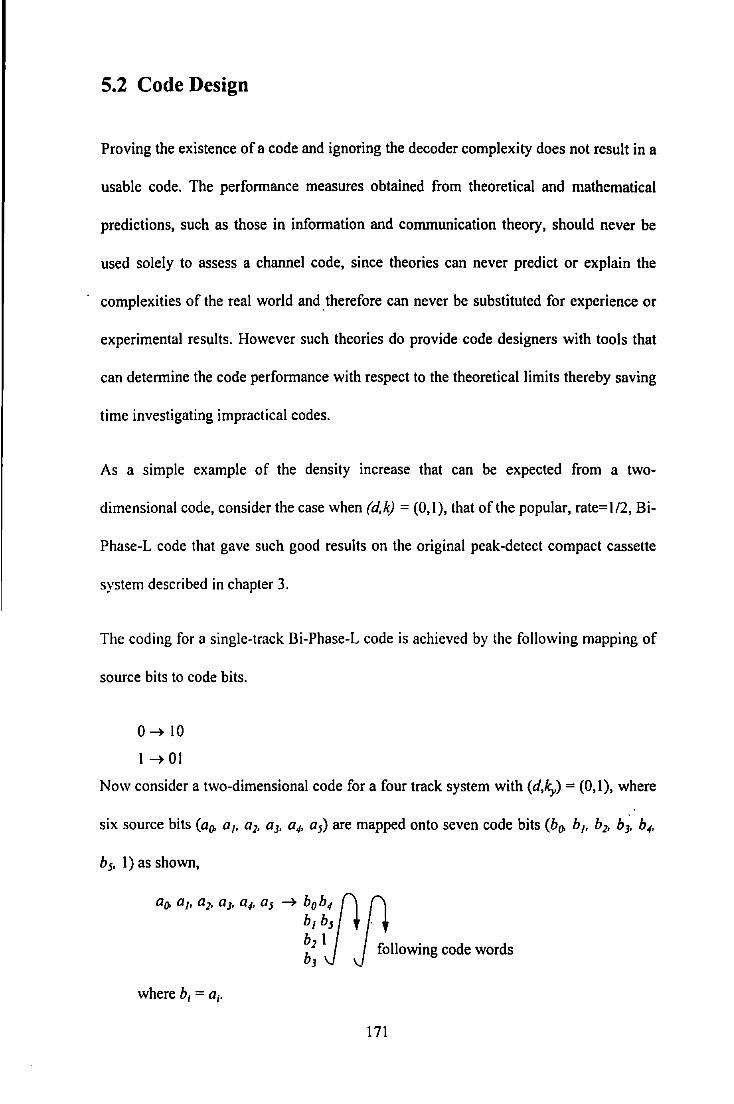
5.2 Code Design

Proving the existence of a code and ignoring the decoder complexity does not result in a

usable code. The performance measures obtained from theoretical and mathematical

predictions, such as those in information and communication theory, should never be

used solely to assess a channel code, since theories can never predict or explain the

complexities of the real world and therefore can never be substituted for experience or

experimental results. However such theories do provide code designers with tools that

can determine the code performance with respect to the theoretical limits thereby saving

time investigating impractical codes.

As a simple example of the density increase that can be expected from a two-

dimensional code, consider the case when (d,k) = {0,1), that of the popular, rate=l/2, Bi-

Phase-L code that gave such good results on the original peak-detect compact cassette

system described in chapter 3.

The coding for a single-track Bi-Phase-L code is achieved by the following mapping of

source bits to code bits.

0--+ 10

1 --+ 01

Now consider a two-dimensional code for a four track system with (d,ls,) = {0,1), where

b 5, 1) as shown,

--+ b0bif:~ bl b5 .

:; 1

following code words

where b1 = a1•

171

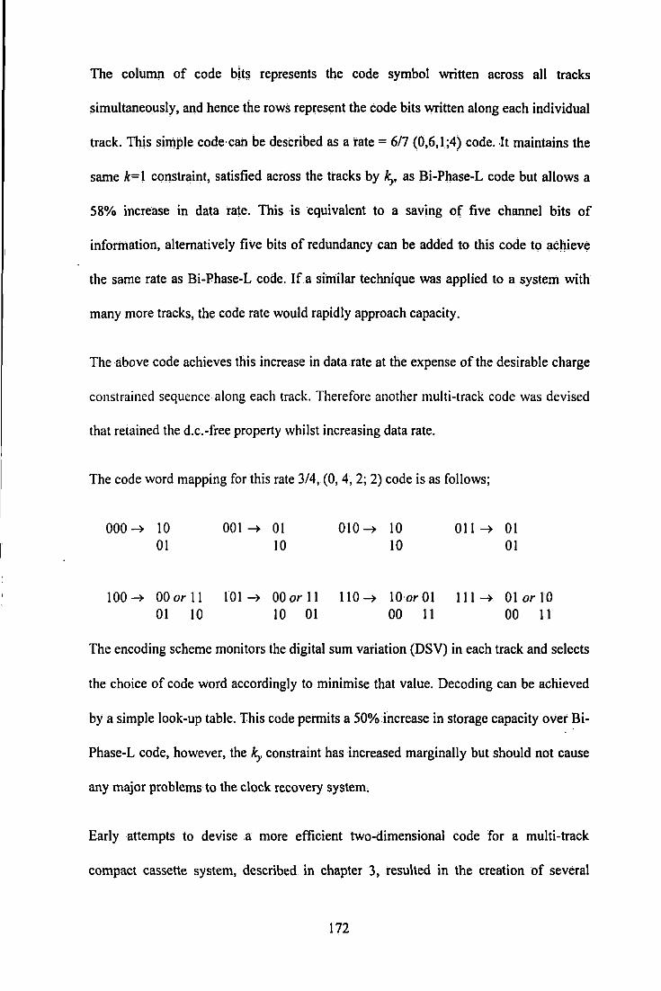
The column of code blts represents the code symbol written across all tracks

simultaneously, and hence the rows represent the code bits written along each individual

track. This simple code·cail be described as a rate = 617 (0,6, 1 ;4) code. It maintains the

same k=l constraint, satisfied across the tracks by Icy as Bi-Phase-L code but allows a

58% increase in data rate. This is equivalent to a saving of five channel bits of

information, alternatively five bits of redundancy can be added to this code to adjieve

the same rate as Bi-Phase-L code. Ifa similar technique was applied to a system with

many more tracks, the code rate would rapidly approach capacity.

The above code achieves this increase in data rate at the expense of the desirable charge

constrained sequence along each track. Therefore another multi-track code was devised

that retained the d.c.-free property whilst increasing data rate.

The code word mapping for this rate 3/4, {0, 4, 2; 2) code is as follows;

000 ~ 10 01

100 ~ OOor 11 01 10

001 ~ 01 10

101 ~ 00 or 11 10 01

010 ~ 10 10

110 ~ 10 or 01 00 11

011 ~ 01 01

Ill~. 01 or 10 00 11

The encoding scheme monitors the digital sum variation (DSV) in each track and selects

the choice of code word accordingly to minimise that value. Decoding can be achieved

by a simple look-up table. This code permits a 50% increase in storage capacity over Bi-

Phase-L code, however, the Icy constraint has increased marginally but should not cause

any major problems to the clock recovery system,

Early attempts to devise .a more efficient two-dimensional code for a multi-track

compact cassette system, described in chapter 3, resulted in the creation of several

172

simple two-dimensional codes, similar to those described above. Most of the

aforementioned codes had a d =0 constraint, however for increased recording density d

> 0 is required. Unfortunately, channel codes that have an increased d constraint usually

require a longer length code word to achieve a code rate close to the capacity. Therefore

more sophisticated two-dimensional coding algorithms were sought.

5.2.1 Capacity of Two-Dimensional Codes

We consider the case when ky < kx since when kx :s; Icy the capacity is less than or equal to

that of a one-dimensional (d,k) code. While [I] allows for ky < d, we assume 0 :s; d :s; Js,.

During each code bit interval, T, one bit must be produced for each track. For simplicity,

we group these bits into a y-tuple which we shall refer to as a code symbol, also called

code vector in [ l ]. Swanson and Wolf [2] calculate the capacity of codes that have both

ky and kx constraints. The k, constraint was included to maintain adequate clock

synchronisation in the event of a burst error to a single track containing all clocking

information (transitions). However, if the coding scheme guarantees transitions

distributed over more than one track the kx constraint could be infinite. Orcutt and

Marcellin [3] describe a method, whereby adding redundancy, any subset of the y

number of tracks can satisfy the ky constraint. The redundancy is given by the number of

defective tracks that can be tolerated, while maintaining synchronisation, without

reduction in the clocking information. Since the kx constraint can be infinite for given

tracks the method to calculate capacity is confined to Icy limited codes.

The states of a multi-track (d, ky; y) code take the form ~{u" u2, ... , uy; v). The value U;

describes the number of consecutive O's in the ;th track and can take on any value in {0,

1, .. , d} with U; = d meaning that d or more consecutive zeros have occurred in the i1h

173

track. Hence, u; monitors the d constraint of the ;rh track. The value v relates to the ky

constraint and indicates the number of consecutive times that all tracks can be 0

simultaneously. Therefore the value v falls in the range {0, l, .. , fs,}. The number of

states, Sj, is calculated as

eqn{l}

The first D = (d + l )" -1 of these states are labelled Sj for j = 0, 1 , ... D, and possess the

associated code symbol cj = (ujb up ..... ujy) which when interpreted as a (d + 1 )-ary

number has decimal value j. The remaining (k -d) states are labelled as SO+; for i = 1, ..

k-d.

The general form of the one-step finite state transition matrix By(d, ky) is given by

By( d. ky) =

s, s,

s, s,

0

....... q ...... · ....... · ....... o ..

·····································: I

... -.............. -.......... . : 0 0 0 0

The sub-matrix ay is given by

174

eqn{2}

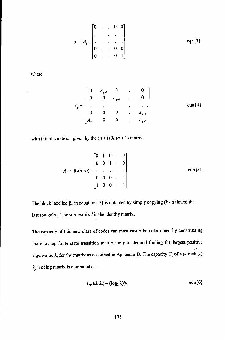
where

a =A -y y

0

0

A = y

0

0

0

0

A,_l

A,_l

0

0

0

0 0

0 0 0

0

A,_l

0

0

0

0

A,_l

A,_l

with initial condition given by the (d +I) X (d + I) matrix

0 I 0 0

0 0 0

A1 = BJ{d, oo) = 0 0 0

0 0

eqn{3}

eqn{4}

eqn{5}

The block labelled ~Y in equation {2} is obtained by simply copying (k- d times) the

last row of ay. The sub-matrix I is the identity matrix.

The capacity of this new class of codes can most easily be determined by constructing

the one-step finite state transition matrix for y tracks and finding the largest positive

eigenvalue /.., for the matrix as described in Appendix D. The capacity Cy of ay-track (d,

ky) coding matrix is computed as:

eqn{6}

175

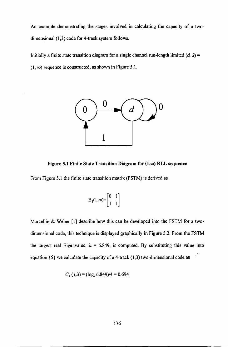
An example demonstrating the stages involved in calculating the capacity of a two­

dimensional (1 ,3) code for 4-track system follows.

Initially a finite state transition diagram for a single channel run-length limited (d, k) =

(1, oo) sequence is constructed, as shown in Figure 5.1.

0

1

Figure 5.1 Finite State Transition Diagram for (l,oo) RLL sequence

From Figure 5.1 the finite state transition matrix (FSTM) is derived as

Marcellin & Weber [I] describe how this can be developed into the FSTM for a two­

dimensional code, this technique is displayed graphically in Figure 5.2. From the FSTM

the largest real Eigenvalue, A. = 6.849, is computed. By substituting this value into

equation {5} we calculate the capacity of a 4-track (1,3) two-dimensional code as -

c4 (1,3) = (log2 6.849)/4 = 0.694

176

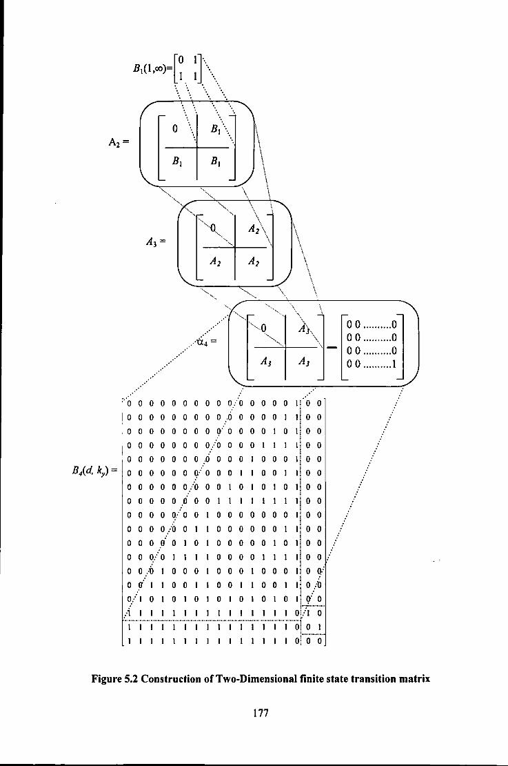
[0 1]-.. B1(1,oo)= \ 1 1 ....

.·

0 •• • ••

·•... ..... ··· ... ··· ...

0

.· .·· .·

·--·-·o --... -.. ____ _

-.... _

.· .· ... ·ii.~·=

A>\ \_

.... __

~-...

\ \

\ \ \

\

;h ...

\

~-..... _

-----''-1--- ·· .. -

'~ 0 0 0 0 0 0 0 0 OjO 0 0 0 0 0 0

looooooooo.ooooo oo o o o o o o o o r o o o o o 1 o o

I 0 0 0 0 0 0 0 OjO 0 0 0 I I I 0 0

0 0 0 0 0 0 0 ~ 0 0 0 I 0 0 0 0 0

Bid, ky) = 0 0 0 0 0 0 q/ 0 0 0 I I 0 0 I I 0 0

o o o o o o./o o o 1 o 1 o o o o 0 0 0 0 0 .fi 0 0 I I I I I I I 0 0

ooooo/oo ooooooo1oo oooo_.:oo oooooo oo 0 0 0 ~ 0 0 0 0 0 0 0 0 0 0

o o o/ o 1 o o o o o o 0 0 :0 0 0 0 0 0 0 0 0 0 I 0 Q.'

I .'

Off 00 OOIIOOIIIO:ll i :

o./10 OIOIOIOIO 01io'o !-7-a-·-

.. ; I I I I I I I I I I I I Oiil 0 ·-····-···-·-·······-···············-----·-·······-···-·····----·········-·············-···-·-··1"

I I I I I I I I I I I I I I I Ol 0 I

I I I I I I I I I I I I I I I Ot 0 0

0 0 .......... 0 0 0 .......... 0 0 0 .......... 0 0 0 .......... 1

Figure 5.2 Construction of Two-Dimensional finite state transition matrix

177

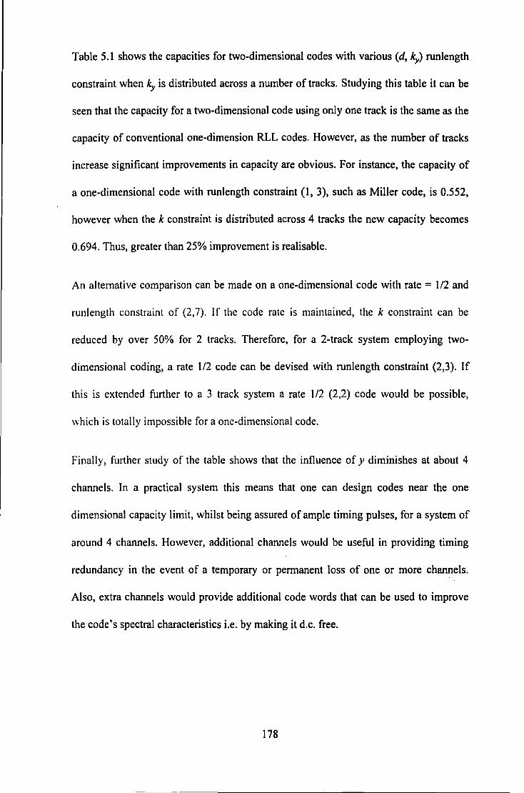
Table 5.1 shows the capacities for two-dimensional codes with various (d, Icy) runlength

constraint when Icy is distributed across a number of tracks. Studying this table it can be

seen that the capacity for a two-dimensional code using only one track is the same as the

capacity of conventional one-dimension RLL codes. However, as the number of tracks

increase significant improvements in capacity are obvious. For instance, the capacity of

a one-dimensional code with runlength constraint (1, 3), such as Miller code, is 0.552,

however when the k constraint is distributed across 4 tracks the new capacity becomes

0.694. Thus, greater than 25% improvement is realisable.

An alternative comparison can be made on a one-dimensional code with rate = 112 and

runlength constraint of (2,7). If the code rate is maintained, the k constraint can be

reduced by over 50% for 2 tracks. Therefore, for a 2-track system employing two­

dimensional coding, a rate 1/2 code can be devised with runlength constraint (2,3). If

this is extended further to a 3 track system a rate 112 (2,2) code would be possible,

which is totally impossible for a one-dimensional code.

Finally, further study of the table shows that the influence of y diminishes at about 4

channels. In a practical system this means that one can design codes near the one

dimensional capacity limit, whilst being assured of ample timing pulses, for a system of

around 4 channels. However, additional channels would be useful in providing timing

redundancy in the event of a temporary or permanent loss of one or more channels.

Also, extra channels would provide additional code words that can be used to improve

the code's spectral characteristics i.e. by making it d.c. free.

178

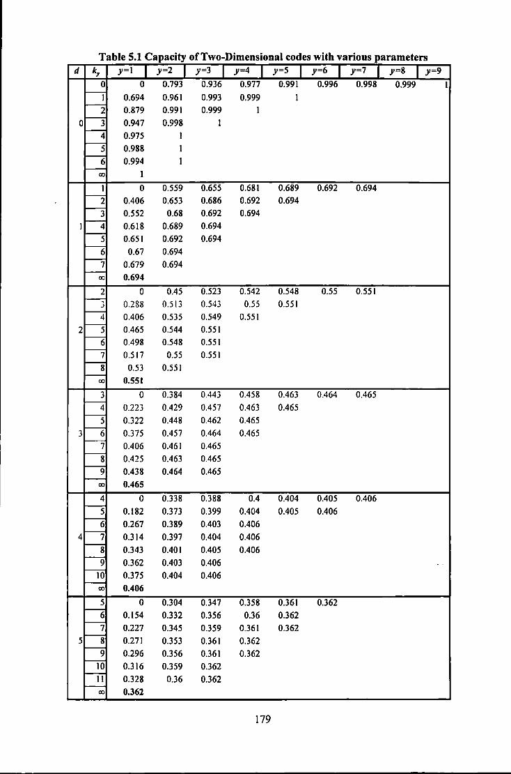
Table 5.1 Capacity of Two-Dimensional codes with various parameters d ky y-1 I y-2 I y-3 I y-4 I y-5 I Y-6 I y-1 I y-8 I y=9

0 0 0.793 0.936 0.977 0.991 0.996 0.998 0.999 I ~ 0.694 0.961 0.993 0.999 I 2 0.879 0.991 0.999 I

o3 0.947 0.998 I

4 0.975 I

5 0.988 I

~ 0.994 I 1--

I <Xl

I 0 0.559 0.655 0.681 0.689 0.692 0.694

~ 0.406 0.653 0.686 0.692 0.694

~ 0.552 0.68 0.692 0.694 I f--;j 0.618 0.689 0.694

~ 0.651 0.692 0.694

~ 0.67 0.694

~ 0.679 0.694 1--

0.694 <Xl

2 0 0.45 0.523 0.542 0.548 0.55 0.551 I--:;-

0.288 0.513 0.543 0.55 0.551 J

f------;j 0.406 0.535 0.549 0.551

2 r------s 0.465 0.544 0.551

~ 0.498 0.548 0.551

~ 0.517 0.55 0.551 f----g 0.53 0.551 1- 0.551 <Xl

3 0 0.384 0.443 0.458 0.463 0.464 0.465 -----;j' 0.223 0.429 0.457 0.463 0.465

-----s 0.322 0.448 0.462 0.465

3~ 0.375 0.457 0.464 0.465

~ 0.406 0.461 0.465 -----g 0.425 0.463 0.465

~ 0.438 0.464 0.465 -<Xl 0.465

4 0 0.338 0.388 0.4 0.404 0.405 0.406

-----s 0.182 0.373 0.399 0.404 0.405 0.406

~ 0.267 0.389 0.403 0.406

4~ 0.314 0.397 0.404 0.406 -----g 0.343 0.401 0.405 0.406

~ 0.362 0.403 0.406 ..

----w 0.375 0.404 0.406 -

<Xl 0.406

5 0 0.304 0.347 0.358 0.361 0.362

~ 0.154 0.332 0.356 0.36 0.362

~ 0.227 0.345 0.359 0.361 0.362 5 -----g 0.271 0.353 0.361 0.362

~ 0.296 0.356 0.361 0.362

----w 0.316 0.359 0.362

IT 0.328 0.36 0.362 -<Xl 0.362

179

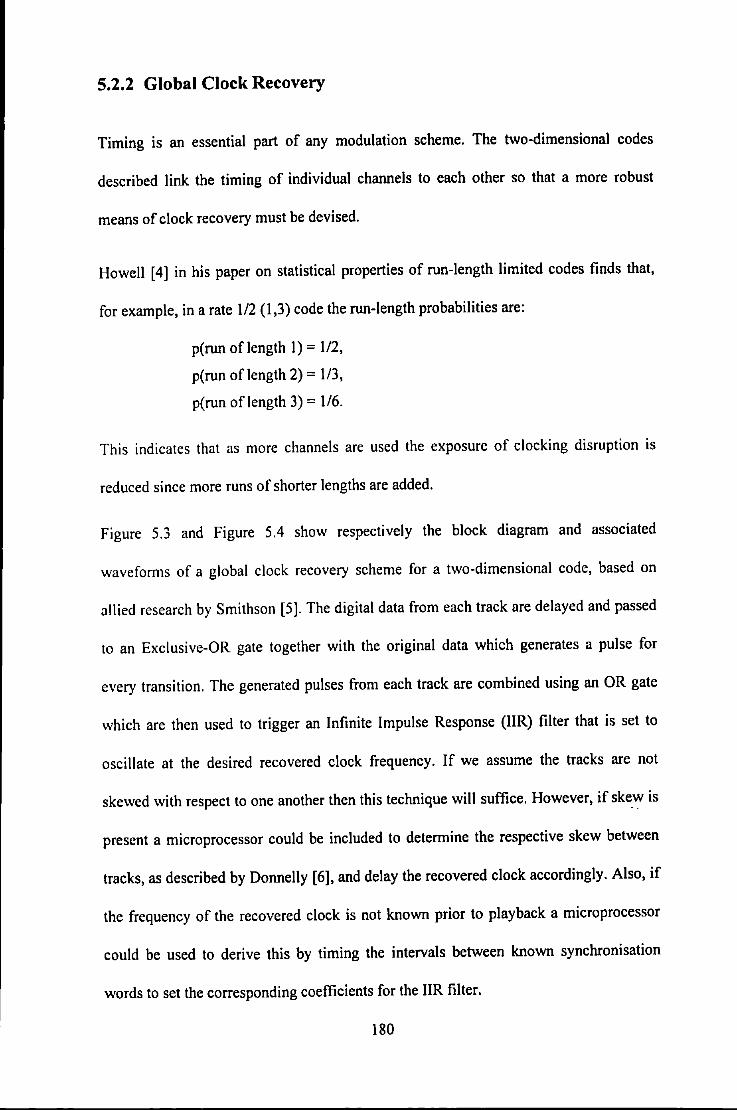
5.2.2 Global Clock Recovery

Timing is an essential part of any modulation scheme. The two-dimensional codes

described link the timing of individual channels to each other so that a more robust

means of clock recovery must be devised.

Howell [4] in his paper on statistical properties of run-length limited codes finds that,

for example, in a rate 1/2 {1,3) code the run-length probabilities are:

p{ run of length I) = 1/2,

p(run of length 2) = 1/3,

p(run of length 3) = 116.

This indicates that as more channels are used the exposure of clocking disruption is

reduced since more runs of shorter lengths are added.

Figure 5.3 and Figure 5.4 show respectively the block diagram and associated

wavefom1s of a global clock recovery scheme for a two-dimensional code, based on

allied research by Smithson [5]. The digital data from each track are delayed and passed

to an Exclusive-OR gate together with the original data which generates a pulse for

every transition. The generated pulses from each track are combined using an OR gate

which are then used to trigger an Infinite Impulse Response (IIR) filter that is set to

oscillate at the desired recovered clock frequency. If we assume the tracks are not

skewed with respect to one another then this technique will suffice. However, if skew is

present a microprocessor could be included to determine the respective skew between

tracks, as described by Donnelly [6], and delay the recovered clock accordingly. Also, if

the frequency of the recovered clock is not known prior to playback a microprocessor

could be used to derive this by timing the intervals between known synchronisation

words to set the corresponding coefficients for the IIR filter.

180

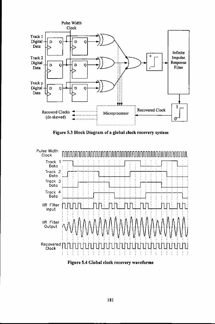
Track 1 Digital Data

Track 2 Digital Data

Track y Digital Data

Pulse Width Clock

.. . . ... . . . . . . . . . ... . . . . . . ... . . . . . . . . . . . .

Infinite Impulse

Response Filter

~,;;~;~:~:;· ;.--R_ec_o_ve_r_ed_C_Io_ck_--1 .J Recoverd Clocks • .. · .......... · ................

(de-skewed) • ............ ..

Figure 5.3 Block Diagram of a global clock recovery system

Pulse Width Clock

Track 1 -----:j Data : : L. --'---'----'--'--'--'

Track 2: j Data :......J

Track 3: Data : ;..-;..._;........l

Track 4: Date

IIR Filter Input

IIR Filter Output

Recovered Clock

Figure 5.4 Global clock recovery waveforms

181

L . .

L

5.3 Two-Dimensional Coding Algorithms

The following methods were investigated as a means to achieve more efficient two­

dimensional codes. All methods have previously been employed for single track codes

but can be extended for multi-track codes. The culmination of this investigation is the

development of a reverse enumeration technique that has several advantages over other

two-dimensional coding algorithms.

5.3.1 Block Coding Technique

Work by Freiman and Wyner [7] on block code constmction for single track codes is the

most easily adapted for two-dimensional codes. By raising the FSTM to the n1h power,

the number of sequences of length n can be calculated for any starting and terminating

states. For each starting state there are a unique set of resulting sequences and a set of

acceptable termination states that produce no constraint violations when sequences are

concatenated.

Consider again the example 4-track (I ,3) code used to illustrate the computation of the

capacity for a two-dimensional code. Figure 5.2 shows the one-step FSTM for this code,

and Figure 5.5. shows the same FSTM raised to the 4th power.

For a starting state of S15 or S16 and termination state of S15, Figure 5.5 shows there are

544 and 529 sequences respectively that satisfy the (1, 3) runlength constraints for a 4-

track code. Therefore nine source bits can be encoded uniquely and without fear of

concatenation, since nine source bits only generate 29 = 512 source sequences. As a

result the channel rate for such a code is 9/16 = 0.5625. As in the case of our example

182

there are usually more code words available than required, In that event any desired

criteria,, such as weight, may be appfiedto.select the 2m code sequences.

s, ·16 i4 24 l6 24 l6 36 54 24 .l6 l6 l4 l6 l4 l4 6l IS 0

24 40 l6 60 l6 60 54 90 l6 60 l4 90· l4 90 81 Ill 22 I

24 36 40 60 l6 l4 60 90 ~6 54' 60 90 l4 81 90 Ill 22 I

l6 60 60 100 l4 9li 90 ISO; 54 9o ·90 ISO 81 'Ill' us 189 l2 l

B/ 24 l6 36 S4 40• 60 60 90 l6 .54 l4 81 '60 90 90 Ill 22 I

36 60 S4 90 60 100 90 ISO S4 90 .81 Ill 90 ISO Ill 189 l2 'l

l6 54' 60 .90 60 90 100 ISO 54 ·81 '90 Ill 90 Ill •llO 189 l2 l

S4 90 9o ISO 90 ISO ISO 250 81 Ill Ill 225 Ill 225 i2S l21 46 ·7

24 36 l6 l4· l6 S4 l4 81 40 60 60 90: 60 90 90 Ill 22

l6 60 54 90 S4 90 81 Ill 60 100 90 ISO 90· HO Ill 189 l2

l6 54 60 90. '54 81 90 Ill 60 90 100 ISO 90 ,IJS· ISO 189 l2 l

54 9o 90 iso si 1135' llS 225 9o ISO ISO 250 Ill. 225 22s lii 46 7 ' l6 l4. 54 81 60• 90 90 Ill 60 90 90 'Ill 100 llO. ISO 189 l2 l '

54 90 ·81 Ill 90· ISO Ill 225 90 ISO Ill 225 ISO llO 225 l21 46 7

l4 81 90 Ill 90 IJS, ISO 225 90 Ill ISO 225 'ISO 225 250 l21 46 7 I s, 80 il4 ll4 224 lj4 224 224 l74 134 224 224 l74' 224 l74 l74 ~65 15! ·s,. 80 Ill Ill 221' Ill 221 221 l67 Ill 221 2H l67 221 l67 l67' 529 65 IS

65 Ill Ill 189 Ill' 189 189 l21 Ill 189 189 ,321: •189 l21 l21 479 so IS'

Fi~ure 5.5 4th Order FSl'M for a 4-track.(1,3) Two-Dimensional' Code

Block coding/decoding is simply achieved with the aid of look up tables, which can be

implemented in hardware via read~only-memory ~ROM). However, to achieve; efficient

codes, with code rate. approaching capacity, _:long code sequences are required. For

instance the example code has: been shown to have a capacity of 0.694, therefore the

above technique produces. a code .that is only 81% efficient. To increase the ·effiCiency

above 95% would require a code length n = 18, with a ·look-up table .containing 218

entries.This·makes.it impractical to use look,up,tables as a means ofencoding/decoding

with c\irrent )rtemory devices. Although it is possible to trade code word length, n,

against an increased Iiwnber of.tracks, y, ;it will still result in a large look-up table Of

impractical proportions. However; :the technique described .is ver.y useful for

determining the number of.available code sequences for a given track density;;)'. and

code word length, n:

183

5.3.2 Sliding Block Technique

The sliding block code construction technique, pioneered by Adler et al. [8], involves

state splitting of the FSTM. Swanson and Wolf [2] provide an excellent detailed

description of how this technique can be applied to a two-dimensional code, therefore

this technique will be dealt with rather briefly high-lighting only the main points of

concern. This technique results in a finite state machine solution to the problem of

encoding, and a combinational logic decoder. Although this process provides a practical

means to encode/decode multi-track codes the method by which the finite state machine

is derived is very complex and does not always yield an optimal solution, therefore

several iterations for the same code generation are sometimes required. Finally, the

example chosen in (2] generates a very simple, inefficient code. Again, by increasing

the efficiency of the code by increasing track density or code word length, the FSTM

becomes very large which drastically increases the complexity involved in deriving the

finite state machine solution.

5.3.3 Enumeration

Recently, Orcutt & Marcellin [9] have described an enumeration technique which is

used to implement a simple two-dimensional code based on a trellis. This scheme

reduces, considerably, the amount of memory required in code implementation with

respect to that of block coding via look-up tables, where memory requirements increase

exponentially with block length. However, this method can be unsuitable for certain

applications since code words with minimal transitions are generated, and no limit has

been placed on the kx constraint.

184

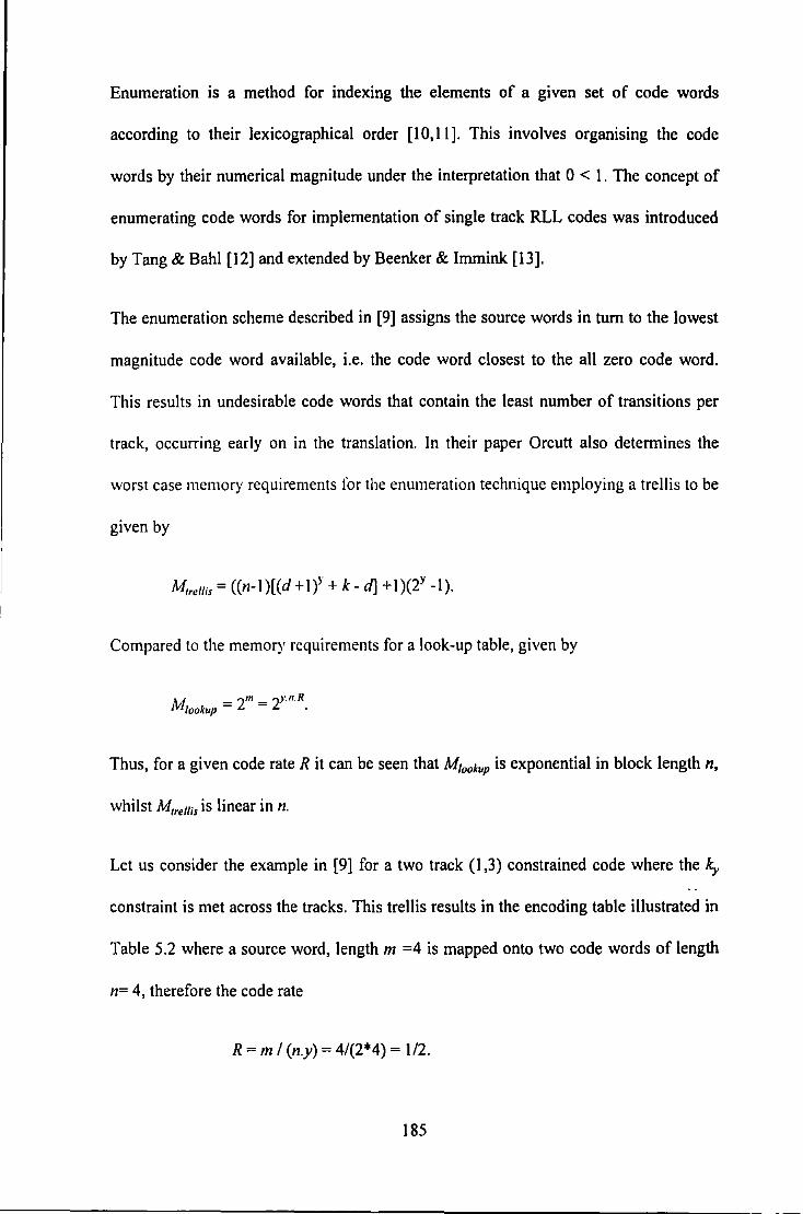
Enumeration is a method for indexing the elements of a given set of code words

according to their lexicographical order [10,11]. This involves organising the code

words by their numerical magnitude under the interpretation that 0 < I. The concept of

enumerating code words for implementation of single track RLL codes was introduced

by Tang & Bahl [12] and extended by Beenker & Imrnink [13].

The enumeration scheme described in [9] assigns the source words in turn to the lowest

magnitude code word available, i.e. the code word closest to the all zero code word.

This results in undesirable code words that contain the least number of transitions per

track, occurring early on in the translation. In their paper Orcutt also determines the

worst case memory requirements for the enumeration technique employing a trellis to be

given by

y y Mire/lis= ((n-l)[(d+l) + k- d] +1)(2 -I).

Compared to the memory requirements for a look-up table, given by

'-1 - 2'" - 2y.n.R fV, lookup - - •

Thus, for a given code rate R it can be seen that Mloolcup is exponential in block length n,

whilst M1rellis is linear inn.

Let us consider the example in [9] for a two track (1,3) constrained code where the Icy

constraint is met across the tracks. This trellis results in the encoding table illustrated in

Table 5.2 where a source word, length m =4 is mapped onto two code words of length

n= 4, therefore the code rate

R =m I (n.y) = 4/(2*4) = 112.

185

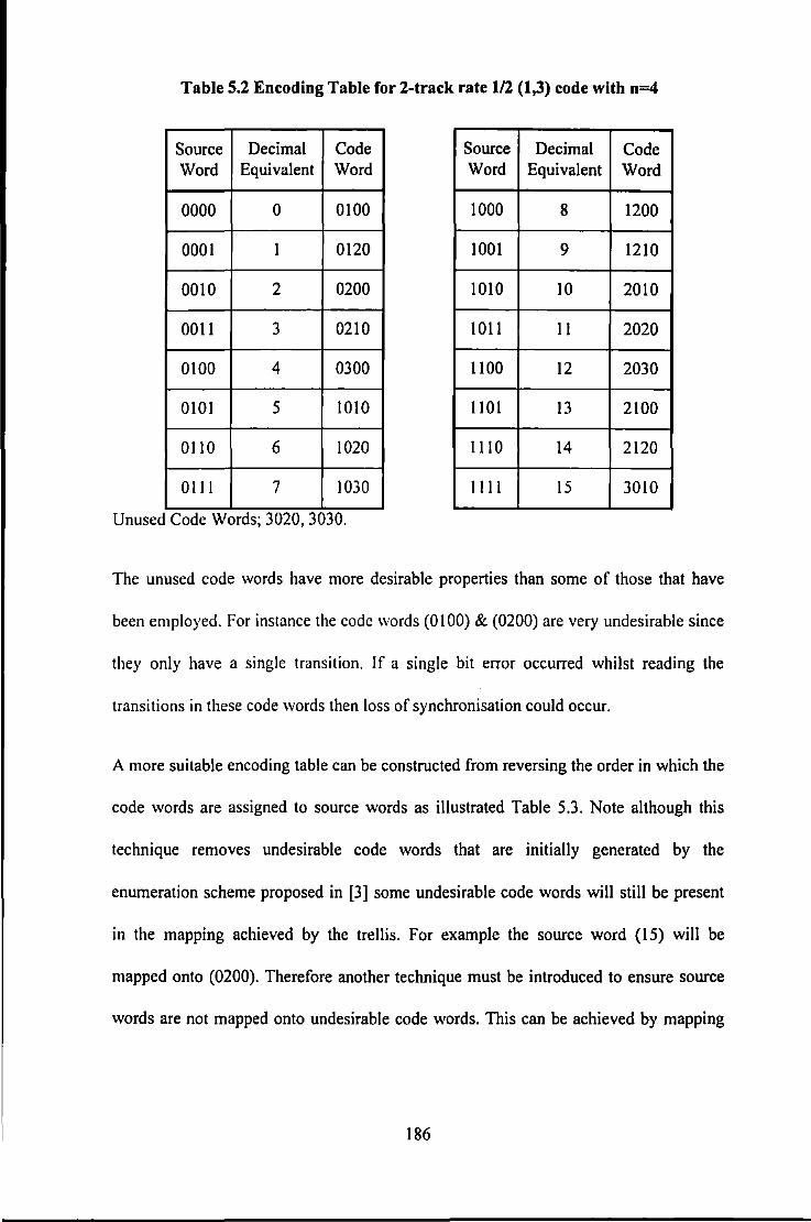
Table 5.2 Encoding Table for 2-track rate 1/2 (1,3) code with n=4

Source Decimal Code Source Decimal Code Word Equivalent Word Word Equivalent Word

0000 0 0100 1000 8 1200

0001 1 0120 1001 9 1210

0010 2 0200 1010 10 2010

0011 3 0210 lOll 11 2020

0100 4 0300 1100 12 2030

0101 5 1010 1101 13 2100

0110 6 1020 Ill 0 14 2120

0 Ill 7 1030 I 11 1 15 3010

Unused Code Words; 3020, 3030.

The unused code words have more desirable properties than some of those that have

been employed. For instance the code words (0100) & (0200) are very undesirable since

they only have a single transition. If a single bit error occurred whilst reading the

transitions in these code words then loss of synchronisation could occur.

A more suitable encoding table can be constructed from reversing the order in which the

code words are assigned to source words as illustrated Table 5.3. Note although this

technique removes undesirable code words that are initially generated by the

enumeration scheme proposed in [3] some undesirable code words will still be present

in the mapping achieved by the trellis. For example the source word (15) will be

mapped onto (0200). Therefore another technique must be introduced to ensure source

words are not mapped onto undesirable code words. This can be achieved by mapping

186

source words onto other out of range source words with more desirable code words.

Therefore source word (IS) can be mapped onto source word (16) prior to enumeration.

Table 5.3 Revised Encoding Table for 2-track rate 112 (1,3) code with n=4

Source Decimal Code Source Decimal Code Word Equivalent Word Word Equivalent Word

0000 0 3030 1000 8 1210

0001 I 3020 1001 9 1200

0010 2 3010 1010 10 1030

0011 3 2120 1011 11 1020

0100 4 2100 1100 12 1010

0101 s 2030 1101 13 0300

0110 6 2020 1110 14 0210

0 Ill 7 2010 1111 IS 0200

10000 16 0120

5.3.4 Reverse Enumeration

The following example demonstrates how reverse enumeration can be employed to

develop a 1/2 rate multi-track code for a 3-track system with constraints d=l and ky=2.

The number of tracks and code word length have deliberately been made small for the

purpose of illustration.

Initially a single-step finite state transition matrix given in Figure S.6a, is constructed, as

described above, to represent legal paths between states. The matrix is raised to

increasing powers until sufficient states are available to achieve a desired code rate.

187

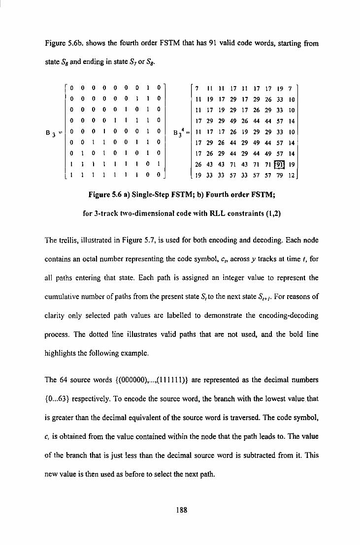
Figure 5.6b. shows the fourth order FSTM that has 91 valid code words, starting from

state Sa and ending in state S7 or Sa.

0 0 0 0 0 0 0 0 1 11 11 17 11 17 17 19 7

0 0 0 0 0 0 0 11 19 17 29 17 29 26 33 10

0 0 0 0 0 0 0 11 17 19 29 17 26 29 33 10

0 0 0 0 I I 0 17 29 29 49 26 44 44 57 14

B3= 0 0 0 0 0 0 0 4 B3 = 11 17 17 26 19 29 29 33 10

0 0 0 0 0 17 29 26 44 29 49 44 57 14

0 0 0 0 0 17 26 29 44 29 44 49 57 14

0 26 43 43 71 43 71 71 f9I) 19

0 0 19 33 33 57 33 51 57 79 12

Figure 5.6 a) Single-Step FSTM; b) Fourth order FSTM;

for 3-track two-dimensional code with RLL constraints {1,2)

The trellis, illustrated in Figure 5.7, is used for both encoding and decoding. Each node

contains an octal number representing the code symbol, c,, across y tracks at time t, for

all paths entering that state. Each path is assigned an integer value to represent the

cumulative number of paths from the present stateS, to the next state Sr+l· For reasons of

clarity only selected path values are labelled to demonstrate the encoding-decoding

process. The dotted line illustrates valid paths that are not used, and the bold line

highlights the following example.

The 64 source words {{000000), ... ,{111111)} are represented as the decimal numbers

{0 ... 63} respectively. To encode the source word, the branch with the lowest value_ that

is greater than the decimal equivalent of the source word is traversed. The code symbol,

c, is obtained from the value contained within the node that the path leads to. The value

of the branch that is just less than the decimal source word is subtracted from it. This

new value is then used as before to select the next path.

188

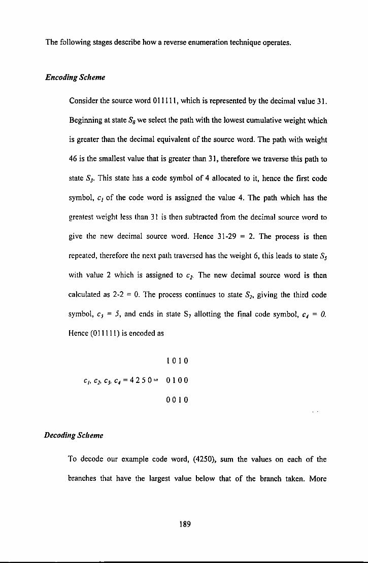
The following stages describe how a reverse enumeration technique operates.

Encoding Sclreme

Consider the source word 011111, which is represented by the decimal value 31.

Beginning at state S8 we select the path with the lowest cumulative weight which

is greater than the decimal equivalent of the source word. The path with weight

46 is the smallest value that is greater than 31, therefore we traverse this path to

state S3. This state has a code symbol of 4 allocated to it, hence the first code

symbol, c1 of the code word is assigned the value 4. The path which has the

greatest weight less than 31 is then subtracted from the decimal source word to

give the new decimal source word. Hence 31-29 = 2. The process is then

repeated, therefore the next path traversed has the weight 6, this leads to state S5

with value 2 which is assigned to c2. The new decimal source word is then

calculated as 2-2 = 0. The process continues to state Sb giving the third code

symbol, c3 = 5, and ends in state S7 allotting the final code symbol, c4 = 0.

Hence (0 Ill I I) is encoded as

l 0 l 0

c1, c2, c3, c4 = 4 2 50= 0 I 0 0

0010

Decoditrg Scheme

To decode our example code word, (4250), sum the values on each of the

branches that have the largest value below that of the branch taken. More

189

simply, sum the values on each of the branches directly above the branch taken.

Where there are no branches above the one traversed just add zero.

Substitution

As previously mentioned, code words with all transitions occurring on a single

track are undesirable, since a burst error whilst reading that track would result in

all timing information being lost. Therefore in our example we wish to prevent

code word (4040) occurring. We achieve this by employing a substitution table,

which prior to encoding, maps the source word onto another, arbitrary, unused

source word that has a more desirable code word. The same table is used

inversely after decoding to regenerate the original source word.

It can be seen from Table 5.4 that in the example code, code word (4040) is

generated by decimal source word 42. Since only sixty four of the ninety one

available code words are used, there are twenty seven remaining code words

from which to chose a substitution. To maintain continuity, a replacement source

word is chosen as 64 which gives a code word (2120).

190

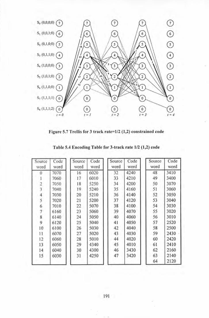
S0 (0,0,0;0) 0 s. {0,0,1;0) 0 S2 eo, 1 ,o;o) 0 S3 co, I , I;O) 0 s4 (I ,o,o;o) ~

Ss (1,0,1 ;0) 0

I = 0

0 0 I= I

0 0 1=2 I = 3

Figure 5.7 Trellis for 3 track rate=l/2 (1,2) constrained code

Table 5.4 Encoding Table for 3-track rate 1/2 (1,2) code

Source Code Source Code Source Code Source word word word word word word word

0 7070 16 6020 32 4240 48 I 7060 17 6010 33 4210 49 2 7050 18 5250 34 4200 50 3 7040 19 5240 35 4160 51 4 7030 20 5210 36 4140 52 5 7020 21 5200 37 4120 53 6 7010 22 5070 38 4100 54 7 6160 23 5060 39 4070 55 8 6140 24 5050 40 4060 56 9 6120 25 5040 41 4050 57 10 6100 26 5030 42 4040 58 11 6070 27 5020 43 4030 59 12 6060 28 5010 44 4020 60 13 6050 29 4340 45 4010 61 14 6040 30 4300 46 3430 62 15 6030 31 4250 47 3420 63

64

191

0 0 0 0 0

I = 4

Code word

3410 3400 3070 3060 3050 3040 3030 3020 3010 2520 2500 2430 . 2420 2410 2160 2140 2120

5.4 Two-Dimensional Coding for EPRML Channels

At this point it is necessary to once again consider the kx constraint imposed along each

individual track. A kx of infinity should not pose a problem to a peak detection channel,

assuming clock synchronisation and automatic gain control can be derived from other

tracks. This is not the case for a channel employing maximum likelihood detection,

where frequent transitions are desirable to force soft decisions.

The d > 0 constrained two-dimensional code produced by the reverse enumeration

scheme can be employed to simplify the extended class IV partial response channel, as

described in chapter 4. The d = 1 constraint removes paths from the EPR4 trellis which

in turn simplifies the number of calculations required for Viterbi detection. However,

the code produced by the reverse enumeration technique does not limit the kx constraint

along each track. A kx = eo constraint can result in no transitions at all occurring on some

tracks, this would make it impossible for the Viterbi detector working on each

individual track to make any decisions. Although, theoretically it should be possible to

construct a Viterbi detector that operated on all or many of the tracks in parallel, this

would result in an immensely large trellis which would dramatically increase the time

and memory required for a practical implementation of such a detector. Therefore, for a

practical implementation it was decided to retain individual Viterbi detectors for each

track.

To re-introduce the kx constraint it was decided to opt for a merging bit solution that

plays a double role. The inclusion of a single charge control bit, P, inserted between

code words on each individual track can be used to bound the DSV and thus make the

code d.c.-free. Making each track d.c.-free has the advantage of effectively introducing a

192

kx constraint along each track. Therefore the Viterbi detector is provided with non-zero

samples to enable path merges, which result in decisions. A null at d.c. is desirable to

match the spectral response of the EPR4 magnetic recording channel.

By monitoring the digital sum variation of two code words, the charge control bit is

chosen to minimise the combined DSV. To prevent the charge control bit violating the d

constraint along each track the following substitutions have to be made.

OOOPO ~valid for all P

OOOPI ~ ifP=1 substitute 00101

0 I OPO ~ valid for all P

0 I OP I ~ if P= 1 substitute 00 I 00

IOOPO ~valid for all P

I OOP I ~ if P= 1 substitute I 0 I 0 I

The technique described above provides a kx constraint and a null at d.c., however this is

at the expense of a reduced code rate. The addition of y charge control bits reduces the

rate of the two-dimensional code too.

Instead of controlling the DSV an odd parity symbol could be used to disperse long run­

lengths of zeros. This would prove more efficient in that it could aid the error detection

scheme. The code rate for such a code is given by

Code Rate R = m/y(n+Np) eqn{7}

where NP is the number of parity bits per track.

However, this must be tolerated in order to benefit from increased density offered by the

combination of extended class IV partial response and maximum likelihood detection.

193

5.4.1 Two-Dimensional rate 1/2 (1,8,2;3) code without D.C. null.

The code described above is only one of many possible variations. For instance a code

with identical run-length constraints that might suit another system that did not require

zero d.c. content along the tracks is described.

From Table 5.4 several code words can be identified that when concatenated would

result in an infinite run-length of zeros on one of the three tracks. Therefore if the source

data resulted in the concatenation of those two-dimensional code words given in the

columns of Table 5.5 one track would contain no transitions.

Table 5.5 Two-dimensional code words without transitions on selected tracks

Track 1 Track 2 Track3 (LSB) (MS B)

6060 5050 3030

6040 5040 3020

6020 SOlO 3010

4240 4140 2420

4200 4100 2120

4060 4050

4020 40!0

There are however a number of replacement code words that allow concatenation

ensuring all tracks posses a transition; these are given in Table 5.6.

194

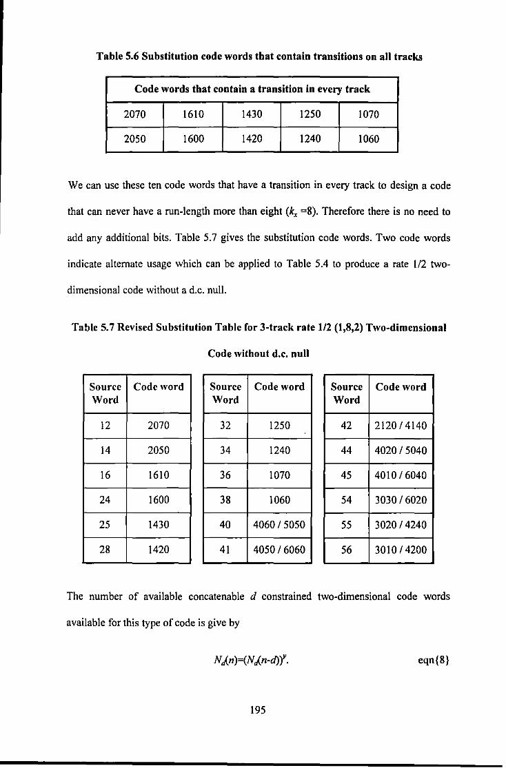
Table 5.6 Substitution code words that contain transitions on all tracks

Code words that contain a transition in every track

2070 1610 1430 1250 1070

2050 1600 1420 1240 1060

We can use these ten code words that have a transition in every track to design a code

that can never have a run-length more than eight (k., =8). Therefore there is no need to

add any additional bits. Table 5.7 gives the substitution code words. Two code words

indicate alternate usage which can be applied to Table 5.4 to produce a rate 112 two-

dimensional code without a d.c. null.

Table 5. 7 Revised Substitution Table for 3-track rate 112 (1,8,2) Two-dimensional

Code without d.c. null

Source Code word Source Code word Source Code word Word Word Word

12 2070 32 1250 42 212014140

14 2050 34 1240 44 4020 I 5040

16 1610 36 1070 45 4010 I 6040

24 1600 38 1060 54 3030 I 6020

25 1430 40 4060 I 5050 55 3020 I 4240

28 1420 41 4050 I 6060 56 3010 I 4200

The number of available concatenable d constrained two-dimensional code words

available for this type of code is give by

NJ..n)=(NJ..n-d)'f. eqn{8}

195

5.5 Combined Error Correction & Modulation

It has been shown that by alleviating the k constraint of the (d ,k) constrained sequences

along each individual track, by sharing the k constraint among many parallel tracks,

codes with increased code rates approaching that of the code capacity can be realised.

Another way of looking at this is, that ones in the code word providing the timing

information in each individual track have been dispersed over many tracks thereby

leaving space for additional information. By increasing the code rate closer to that of its

capacity means that the additional information stored in a code word relates to that of

the source data. However this could be replaced with error correction information, that

would strengthen the code's ability to detect and correct any errors that may have

occurred in recording, whilst maintaining a constant code rate. If enough tracks were

available, a code could be constructed to have a rate approaching that of its capacity as

well as containing error correction information. One such application where this type of

coding would be of benefit is a stationary head video recorder with several hundred

tracks to disperse information over [14,15].

For example take a simple 1/4 rate (1,3) code, where the source data, x, bit is mapped on

to the first bit of the code word, and the following bits of the code word maintain the d

and k constraints. The third bit of the code word is always 1 to maintain the k constraint

along the track that provides timing information.

x~xOlO

196

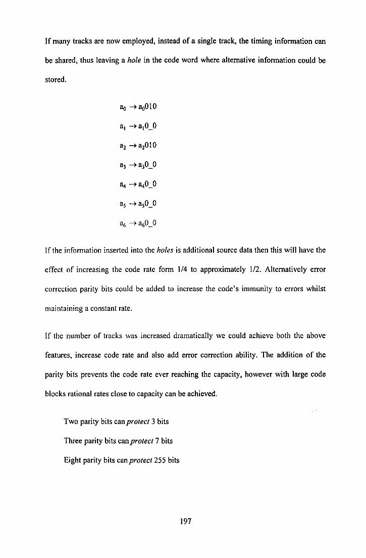
If many tracks are now employed, instead of a single track, the timing information can

be shared, thus leaving a hole in the code word where alternative information could be

stored.

ao --+ aoOIO

al --+ alo_o

a2 --+ a201 0

a3 --+ a30_0

a4 --+ a40_0

a5 --+ a50_0

a6 --+ a60_0

If the information inserted into the holes is additional source data then this will have the

effect of increasing the code rate form 1/4 to approximately 112. Alternatively error

correction parity bits could be added to increase the code's immunity to errors whilst

maintaining a constant rate.

If the number of tracks was increased dramatically we could achieve both the above

features, increase code rate and also add error correction ability. The addition of the

parity bits prevents the code rate ever reaching the capacity, however with large code

blocks rational rates close to capacity can be achieved.

Two parity bits can protect 3 bits

Three parity bits can protect 7 bits

Eight parity bits can protect 255 bits

197

It can be seen that the number of bits, N0 , protected by addition of parity bits grows

exponentially with the following equation

for p > 1 eqn{9}

where p is the number of parity bits.

However, the number of code bits, Nb, increase linearly with the addition of each track

eqn{10}

where y is the number of tracks, n is the code word length.

For a single bit error correcting code the number of bits protected by parity must be

greater than or equal to the total number of bits in all code words.

eqn{l1}

substituting equations {9} & { 10} in { 11} gives

eqn{12}

The rate of a code is given by

R = m/n.y eqn{ 13}

The number of combinations of a binary source word of length m is 2m.

The total number of combinations of a binary code word of length n, constrained by d is

g1ven as

N,l.,n) = n+! for 1~n ~ d+1 eqn{ 14}

198

NJ..n) = NJ..n-1) + NJ..n-d-1) for n > d+1 eqn{l5}

However for concatenable, d constrained code words the total number of combinations

is reduced to

N£n -d) eqn{16}

For successful code realisation.

eqn{l7}

eqn{18}

Substituting { 18} in { 13} we get the maximum rate of a code is

R = mln = log2 Nd(n-d)ly.n eqn{l9}

If we now add the number of parity bits required for a single bit error correcting code

we obtain an expression relating maximum rate to the number of tracks, y, and the code

word length n.

eqn{20}

5.6 Discussion

Two-dimensional modulation codes and how such codes can be used to increase the

overall capacity of a multiple track digital recording system are presented. The capacity

of several codes has been determined and shows improved performance over

conventional one-dimensional RLL codes. The issue of global clock recovery for such

codes has been addressed and a method based on digital filtering is described. Although

199

such a scheme has yet to be implemented in practice, simulation on a single track has

shown enhanced performance over software techniques previously employed by the

author. Various encoding techniques have been detailed including a new reverse

enumeration scheme. Example two-dimensional codes for system employing extended

partial response and maximum likelihood detection are constructed using a reverse

enumeration scheme. These codes have the added ability to either match the d.c. null

spectral response of magnetic recording channel or incorporate error detection

information in the form of parity bits.

A method of constructing multiple-track RLL block codes, implemented using a reverse

enumeration scheme based on the trellis description of the constraints has also been

proposed. This scheme results in a complexity which varies only linearly with block

length as opposed to the exponential relationship exhibited by a look-up table

implementation. This method is rather elegant in its simplicity and requires no

knowledge of the code words since all relevant information is contained within the

trellis which is relatively easy to construct. However, the state-splitting technique for

creating trellis codes generally produce codes which are more efficient and exhibit less

error propagation. This result should not be surprising since trellis codes use a greater

number of sequences which satisfy the (d, k) constraints than block codes do. This is

because block codes are state independent while trellis codes are not. The one thing the

enumerable block codes have in their favour is ease of construction and implementation.

Since the state partitioning/splitting process performed in construction of trellis codes

can be tedious and time consuming, especially when trying to achieve codes near

capacity, and the resultant encoder/decoder is generally not trivial.

200

5. 7 References

1. Marcellin, M.W., & Weber, H.J., "Two Dimensional Modulation Codes", IEEE J.

Sel. Areas in Comms., Vol.1 0, No.1, pp.254-66, January 1992.

2. Swanson, R.E., & Wolf, J.K., "A New Class of Two-Dimensional RLL Recording

Codes", IEEE Trans. Magn., Vol.28, No.6, pp.3407-16, November 1992.

3. Orcutt, E.K., & Marcellin, M.W., "Redundant Multitrack (d,k) Codes", IEEE Trans.

Inf. Theory, Vol.39, No.S, pp.1744-50, September 1993.

4. Howell, T.D., "Statistical Properties of Selected Recording Codes", IBM J. Res.

Develop., Vol.33, No.1, pp.60-73, January 1989.

5. Smithson, P.M., Tomlinson, M., & Donnelly, T., "Clock Recovery using IIR filter",

to be presented at Globecom '94, (San Francisco, CA), November 1994.

6. Donnelly, T., "Real Time Microprocessor Techniques for a Digital Multitrack Tape

Recorder", PhD Thesis, University of Plymouth, 1989.

7. Freiman, C.V., & Wyner, A.D., "Optimum Block Codes for Noiseless Input

Restricted Channels", Information and Control, Vol.7, pp.398-415, 1964.

8. Adler, R., Hassner, M., Kitchens, & Moussouris, P., "Method and Apparatus for

Generating Sliding Block Code for a (1,7) Channel with Rate 2/3", US Patent

4,413,251., I November 1983.

9. Orcutt, E.K., & Marcellin, M.W., "Enumerable Multitrack (d,k) Block Codes",

IEEE Trans. Inf. Theory, Vol.39, No.S, pp.1738-44, September 1993.

10. Cover, T.M., "Enumerative Source Encoding", IEEE Trans. lnf. Theory, Vol.l9,

No.1, pp.73-77, January 1973.

11. Slake, I. F., "The Enumeration of Certain Run Length Sequences", Information and

Control, Vol.55, pp.222-37, 1982.

201

12. Tang, D., & Bahl, L., "Block Codes for a Class of Constrained Noiseless

Channels", Information and Control, Vol.l7, pp.436-61, 1970.

13. Beenker, G.F.M., & Immink, K.A.S., "A Generalized Method for Encoding and

Decoding Run Length Limited Binary Sequences", IEEE Trans. Inf. Theory,

Vol.29, No.S, pp.751-54, September 1983.

14. Maurice, F., "Towards the Multitrack Digital Video Tape Recorder", Proceedings

ofMORIS '91.

15. Mailliot, C., & Maurice, F., "The Kerr Head: A Multitrack Fixed Active Head",

IEEE Trans. Magn., Vol.28, No.S, pp.2656-58, September 1992.

202

CHAPTER6

Conclusions & Further Work

6.1 Conclusions

The impetus behind the infonnation storage industry is to increase the storage capacity

of devices for minimum cost. In magnetic recording this means increasing the area! bit

packing density by increasing track density resulting from reducing space between and

width of the recording tracks, and/or reducing the wavelength of the recorded

infonnation.

The aim of this research was to offset the mechanical vagaries of a low-cost tape

transport and tape, such as the compact-cassette fonnat, by sophisticated software signal

processing and coding techniques. The problem of low signal to noise ratios and high

error rates may be alleviated by the use of more sophisticated coding schemes and signal

processing techniques.

The ultimate limits of magnetic recording cannot be reached without sophisticated

signal processing and coding techniques. The theme of this dissertation has been to

investigate the degree to which channel coding can help reach those limits.

203

The author initially interfaced a first generation digital signal processor to a standard

compact cassette mechanism to form a basic multiple-track digital magnetic tape storage

system. Software written in TMS320 I 0 assembly language was developed by the author

to control the recording system's functions, such as channel encoding/decoding and data

synchronisation, to maintain the low cost. Also, parallel software algorithms were

developed which permit each track to be processed concurrently. Several RLL

modulation codes were applied to the system and the error rates for a range of data rates

were measured. By including a high speed digital signal processor new techniques were

developed to more accurately derive the best sampling point to minimise errors caused

by skew. A trailing edge detection process, developed by the author, used for Bi-Phase­

L code gave an improvement over results obtained on a similar system by Donnelly.

From the results of this system it was shown that greater efficiency codes do not always

perform as well as predicted. This is because the coding has to be matched to the

vagaries of the system and detection process as well as the channel bandwidth. Further,

an oversample read technique was developed and implemented to completely eliminate

azimuth errors. This technique highlighted the need for post-equalisation to limit the

effects of inter-symbol interference

In the second phase of research a new system was developed by the author that had a

faster digital signal processor and replaced the hard limiting peak detectors with

analogue to digital converters. Equalisation was employed using a simple 5-tap Finite

Impulse Response (FIR) filter that slimmed the readback signal by approximately 30%.

The improvement in pulse width was translated into a corresponding increase in data

rate for a given error rate. However, it was noted that equalisation techniques also boost

204

the high frequency noise and therefore there is a limit as to how much equalisation can

be applied without dramatically reducing the signal-to-noise ratio.

Partial Response signalling techniques, that introduce a controlled amount of inter­

symbol interference to shape the readback pulse, were proposed as an alternative

method of increasing recording density to pulse slimming that tries to remove ISI. In

particular PR4 and EPR4 techniques, that have spectral nulls at d.c and the Nyquist

frequency, were identified as having spectral response similar to the magnetic recording

channel.

However, partial response techniques produce multi-level signals and hence also reduce

the signal to noise ratio. Therefore Maximum Likelihood sequence detection was

proposed that makes deferred decisions on the outcome of a signal instant by

considering the relative position in a sequence rather than symbol-by-symbol detection

of the peak detector. Maximum Likelihood sequence detection is a computationally

intensive task that requires high speed processors to perform the calculations in real

time. Recent advances in silicon technology have only now permitted PRML to be

considered as a viable alternative to the analogue peak detector.

Investigation into PRML for the magnetic recording channel showed that spectral

requirements of the PR4 detector can be satisfied over a range of recording densities by

suitable equalisation of the readback signal. Beyond that range, however, noise

enhancement penalty in equalisation and the lower signal to noise ratio due to peak

power limitation of the channel cause the input SNR to the ML detector to drop below

the theoretical level for acceptable performance. Further increase in recording density

may be achieved by using a class of partial response that is more closely matched to the

205

readback signal, thereby reducing the noise enhancement penalty in equalisation.

However, due to the increased number of levels in higher orders of partial response the

effective SNR at the detector is reduced, although the Viterbi algorithm can recoup

some loss through redundant output levels inherent due to correlation in the partial

response signal. If we ignore the fact that the complexity of the Viterbi detector

increases exponentially with number of output levels then equalising to extended class

IV partial response is the best choice for high linear recording densities. EPR4 also has

the advantage of permitting d> 1 constrained codes that can be used to simplify the

Viterbi detection algorithm.

Conventional coding schemes designed for the peak detect channel are not well suited to

channels employing PRML. Therefore a new breed of trellis codes for PRML channels

have recently attracted much attention. Trellis codes such as the Matched Spectral Null

code give a 3dB coding gain over uncoded sequences, as well as matching the spectrum

of digital magnetic channel. Several coding schemes for the magnetic PRML channel

were investigated by the author and the associated advantages and disadvantages have

been discussed.

Whilst the above techniques significantly increase density along the tracks few attempts

have been made to benefit from the redundancy introduced by a multiple-track system.

Therefore, the author concentrates the final stage of research on investigating coding

techniques that exploit the redundancy of the multi-track recording system.

A method to generate concatenable block codes for arbitrary y-track (d. icy) two

dimensional codes is proposed. The resultant code is implemented via a reverse

enumeration scheme, developed by the author, based on a trellis which contains all

206

relevant infonnation about the code words. This allows both encoding and decoding to

be executed without explicit knowledge of these code words. The advantage of this

scheme over a look-up table implementation is in the amount of memory required. For a

look-up table approach, memory increases exponentially for increased code block length

n whilst using a trellis approach memory only increases linearly with n.

This work has been furthered by the author through the development of a coding

technique that produces two-dimensional code words with an increased number of non­

zero bits. This technique is desirable for a multi-track magnetic recording system since

it results in a higher average number of transitions per code symbol. This is

advantageous for two reasons:

a) It provides more infonnation to the clock recovery system, this can be used

for either reducing the complexity of the clock recovery algorithm or

detennining a de-skew technique.

b) It reduces the amount of path memory required in a system employing

maximum likelihood sequence detection using the Viterbi algorithm, since

transitions cause the paths through the trellis to converge.

A simple two-dimensional code described in chapter 5 has been specifically designed

as an example to match several characteristics found in a high density compact

cassette system. The ky constraint has been deliberately made small in an effort to

duplicate the perfonnance of Bi-Phase-L code by limiting the number of ratios for

synchronisation. The author proposed that PRML would be used in a high density

digital magnetic recorder, therefore a d= l constraint has been imposed on the code

207

primarily to simplify the Viterbi detection by reducing the number of states in the

trellis.

A technique has also been described to make the code d.c.-free in an aim to match the

spectral characteristics of both EPR4 and the magnetic recording channel. Only

experimentation will determine if the sacrifice of reduced capacity through the

addition of the an extra bit in each track to control the d.c.-content, yields an overall

improved performance. If the d.c.-free constraint is not required then an alternative

two-dimensional code has also been developed.

6.2 Further Work

The research carried out for this thesis has generated a substantial amount of potential

further work, described below.

The two-dimensional codes developed in this investigation were developed for a multi­

track system employing extended class IV partial response signalling with maximum

likelihood detection. Because of time constraints it was not possible to develop a system

employing EPRML. This would entail the development of several crucial procedures

such as: automatic gain control (AGC), to ensure the playback signal from a variety of

different tapes is of equal amplitude; channel equalisation equally distributed between

both the write and read process with the post equalisation preferably employing some

adaptive equalisation; and also a more effective clock recovery scheme. All these tasks

could be accomplished using sophisticated software which would require considerable

development. Indeed an allied research project into software clock recovery is in

progress.

208

The sampling detection system developed in this investigation was designed to facilitate

the addition of several processor boards capable of working concurrently on individual

signal processing tasks and sharing information. It would therefore be possible to use

this system as a platform on which to build a multi-track digital tape recorder with a

completely adaptive software channel. However, as more advanced high-speed parallel­

processing DSP devices, such as the TMS320C40, become more readily available using

such a device may prove a more cost effective solution, since a single device has greater

than ten fold increase in computational speed.

Finally, all techniques developed in this investigation are for parallel operation and may

be applied to any track density provided a microprocessor of comparable word length is

employed. If an adequate signal to noise ratio can be maintained, thin-film, magneto­

resistive read/write recording heads can be applied with higher track densities. A Philips

Digital Compact Cassette recorder has been purchased for the next phase of the

investigation. The application of two-dimensional coding with EPRML should yield

increased data rates. Also higher track density heads produced for a stationary head

digital video recorder will permit further exploration into this area. This will allow

further exploration into the possible advantages and disadvantages of higher track

densities. Other signal processing algorithms are sure to be developed as a result of

such an investigation.

209

,.

Appendix />I.

presented! at:

Euromicro'92 !Conference,

Paris, France; 1992.

&

11EEE'. Inteniaiion Magnetics Conference ('Intennag':94),

Albuquer:que, N:M., U.S.A., 1994_:

Al

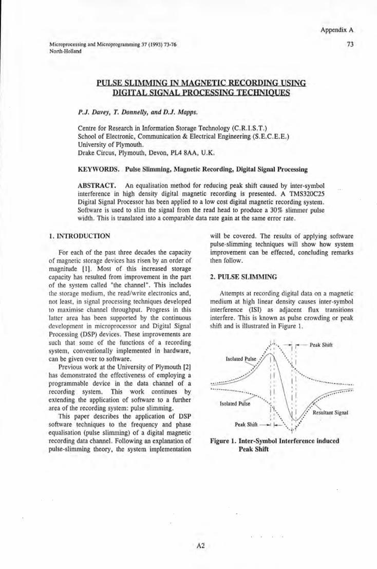
Appendix A

Microprocessing and Microprogramming 37 {1993) 73-76 Nonh-Holland

PULSE SLIMMING IN MAGNETIC RECORDING USING DIGITAL SIGNAL PROCESSING TECHNIQUES

P.J. Davey, T. Don11elly, and D.J. Mapps.

Centre for Research in Information Storage Technology (C.R.l.S.T.) School of Electronic, Communication & Electrical Engineering (S.E.C.E.E.) University of Plymouth. Drake Circus, Plymouth, Devon, PIA 8AA, U.K.

KEYWORDS. Pulse Slimming, Magnetic Recording, Digital Signal Processing

ABSTRACT. An equalisation method for reducing peak shift caused by inter-symbol interference in high density digital magnetic recording is presented. A TMS320C25 Digital Signal Processor has been applied to a low cost digital magnetic recording system. Software is used to slim the signal from the read head to produce a 30% slimmer pulse width. This is translated into a comparable data rate gain at the same error rate.

73

1. INTRODUCTION

For each of the past three decades the capacity of magnetic storage devices has risen by an order of magnitude [I]. Most of this increased storage capacity has resulted from improvement in the part of the system called "the channel". This includes the storage medium, the read/write electronics and, not least, in signal processing techniques developed to maximise channel throughput. Progress in this latter area has been supported by the continuous development in microprocessor and Digital Signal Processing (DSP) devices . These improvements are such that some of the functions of a recording system, conventionally implemented in hardware, can be given over to software.

will be covered. The results of applying software pulse-slimming techniques will show how system improvement can be effected, concluding remarks then follow.

Previous work at the University of Plymouth [2] has demonstrated the effectiveness of employing a programmable device in the data channel of a recording system. This work continues by extending the application of software to a further area of the recording system: pulse slimming.

This paper describes the application of DSP software techniques to the frequency and phase equalisation (pulse slimming) of a digital magnetic recording data channel. Following an explanation of pulse-slimming theory, the system implementation

A2

2. PULSE SLIMMING

Attempts at recording digital data on a magnetic medium at high linear density causes inter-symbol interference (ISI) as adjacent flux transitions interfere. This is known as pulse crowding or peak shift and is illustrated in Figure I.

I , . . ··· ·. - - r - Peak Shaft .• , I · , I

Isolated Pulse _ ..... • ' \._ : '

''I.~ I ........ .·

'' , I ···-..... I I . . .... .. . .. _ ... ..

' ' -----................ _ 11 ~· · ... ..

Isolated Pulse • ·~ ' 1'1.. :: ... ,.t I I t '"

Peak Shift -----1 1--\ • ~:' .. ,., Resultant Signal

Figure 1. Inter-Symbol Interference induced Peak Shift

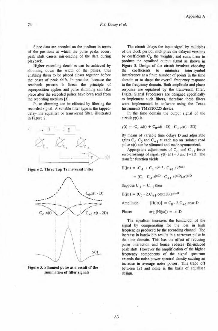
Appendix A

74 P.J. Davtry et al.

Since data are encoded on the medium in terms of the positions at which the pulse peaks occur, peak shift causes mis-reading of the data during playback.

Higher recording densities can be achieved by slimming down the width of the pulses, thus enabling them to be placed closer together before the onset of peak shift. In practice, because the readback process is linear the principle of superposition applies and pulse slimming can take place after the recorded pulses have been read from the recording medium [3].

Pulse slimming can be effected by ftltering the recorded signal. A suitable filter type is the tapped­delay-line equaliser or transversal filter, illustrated in Figure 2.

'·' ------,

D - . D

3 B' .

c C · I 0 0 C · I

----3>--y(tJ

Figure 2. Three Tap Transversal Filter

~,

I \ I \

I \ I \

/ ' / , C0.x(t- D) ~;~/ ',,~ ---- -....... __

::::::::··············· ...... !. .... ·:: ........ . ·•·•.• I ·:~-::· ,.··

c _l.x(t) ··......... ·• ......... c + l .x(t - 2D)

y(t)

Figure 3. Slimmed pulse as a result of the summation of filter signals

A3

The circuit delays the input signal by multiples of the clock period, multiplies the delayed versions by coefficients Ci, the weights, and sums them to produce the equalised output signal as shown in Figure 3. Design of the circuit involves choosing the coefficients to mtrumtse inter-symbol interference at a ftn.ite number of points in the time domain or to shape the overall frequency response in the frequency domain. Both amplitude and phase response are equalised by the transversal filter. Digital Signal Processors are designed specifically to implement such filters, therefore these filters were implemented in software using the Texas Instruments TMS320C25 device.

In the time domain the output signal of the circuit y(t) is

By means of variable time delays D and adjustable gains C _1 C0 and C + 1 at each tap an isolated read pulse x(t) can be slimmed and made symmetrical.

Appropriate adjustments of C_1 and C+ 1 force zero-crossings of signal y(t) at t=O and t=2D. The transfer function yields

HUro) = -C-1 + Co.e·jwD- c + t·e·j2wD

= (Co- C. t ·~ruD - C+ t·e·jruD).e-jwD

Suppose C_1 = C+t then

HUro) = (C0 • 2.C+ 1.cosroD).e-jwD

Amplitude:

Phase:

IHUro)l = C0 - 2.C+ 1.cosroD

arg (HUro)) = -ro. D

The equaliser increases the bandwidth of the signal by compensating for the loss in high frequencies produced by the recording channel. The increase in bandwidth results in a narrower pulse in the time domain. This has the effect of reducing pulse interaction and hence reduces · ISI-induced peak shift. However the amplification of the higher frequency components of the signal spectrum extends the noise power spectral density causing an increase in average noise power. This trade off between ISI and noise is the basis of equaliser design.

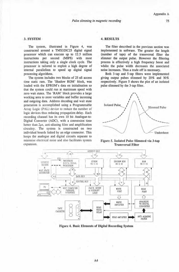
Appendix A

Pulse slimming in magnetic recording 75

3. SYSTEM

The system, illustrated in Figure 4, was constructed around a TMS320C25 digital signal processor which can execute up to 12.5 million instructions per second (MIPS) with most instructions taking only a single clock cycle. The processor is tailored to exploit a high degree of internal parallelism to speed up digital signal processing algorithms.

The system includes two blocks of 25 nS access time static ram. The 'Shadow ROM' block, was loaded with the EPROM's data on initialisation so that the system could run at maximum speed with zero wait states. The 'RAM' block provides a large working area to store variables and buffer incoming and outgoing data. Address decoding and wait state generation is accomplished using a Programmable Array Logic (PAL) device to reduce the number of logic devices thus reducing propagation delay. Each recording channel has its own 10 bit Analogue-to­Digital Converter (ADC), with a conversion time better than 2ps, anti-aliasing filter and amplification circuitry. The system is constructed on two individual boards linked by an edge connector. This keeps the analogue and digital circuits separate to minimise electrical noise and also facilitates system expansion.

-7

IOO~E:~5

4. RESULTS

The ftlter described in the previous section was implemented in software. The greater the length (number of taps) of the transversal filter the slimmer the output pulse. However the filtering process is effectively a high frequency boost and whilst the pulse width decreases the associated noise increases. Thus a trade off is necessary.

Both 3-tap and 5-tap fillers were implemented giving output pulses slimmed by 20% and 30% respectively. Figure 5 shows the plot of an isolated pulse slimmed by the 3-tap filter.

, ..... , I

I I

Isolated Puls'--t/

,-' ------"

I I ,

I Sl immed Pulse

' ' ' ........ _ ----- .

Undershoot

Figure 5. Isolated P ulse Slimmed via 3-tap Transversal Filter

1:;~f:;~ ~"',I_--___ "" ""'-=-=--=:-:-:-::----->..... r--t-------=' ,..y----~

TAPE CASSETIE

0 0 0

0

Figure 4. Basic Elements of Digital Recording System

A4

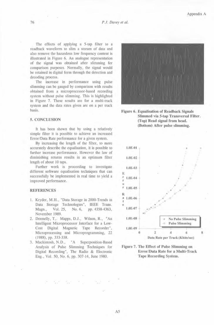
Appendix A

76 P.J. Davey et al.

The effects of applying a 5-tap filter to a readback waveform to slim a stream of data and also remove the hazardous low frequency content is il lustrated in Figure 6. An analogue representation of the signal was obtained after slimming for comparison purposes. Normally, the signal would be retained in digital form through the detection and decoding process.

The increase in performance using pulse slimming can be gauged by comparison with results obtained from a microprocessor-based recording system without pulse slimming. This is highlighted in Figure 7. These results are for a multi-track system and the data rates given are on a per track basis.

5. CONCLUSION

rt has been shown that by using a relatively simple filter it is possible to achieve an increased Error/Data Rate performance for a given system.

By increasing the length of the filter, to more accurately describe the equalisation, it is possible to further increase performance. However the law of diminishing returns results in an optimum ftlter length of about lO taps.

Further work is proceeding to investigate different software equalisation techniques that can successfully be implemented in real time to yield a improved performance.

REFERENCES

1. Kryder, M.H., "Data Storage in 2000-Trends in Data Storage Technologies", IEEE Trans. Magn., Vol. 25, No. 6, pp. 4358-4363, November 1989.

2. Donnelly, T,. Mapps, D.J., Wilson, R., "An Intelligent Microprocessor Interface for a Low­Cost Digital Magnetic Tape Recorder", Microprocessing and Microprogramming, 22 ( 1988), pp. 333-338.

3. Mackintosh, N.D., "A Superposition-Based Analysis of Pulse Slimming Techniques for Digital Recording" , The Radio & Electronic Eng., Vol. 50, No. 6, pp. 307-14, June 1980.

A5

Figure 6. Equalisation of Readback Signals Slimmed via 5-tap Transversal Filter. (Top) Read signal from head. (Bottom) After pulse slimming.

J.OE-01

J.OE-02

I.OE-03

E r I.OE-04 r 0

r J.OE-05

R a I.OE-06 t

e I.OE-07 j

t.OE-08

l.OE-09 0 2

/ I

" ,

•' a

I I

I ,

' ,0

•

I

0

'

I

I

No Pu lse Slimming Pulse Slimming

4 6

Data Rate per Track (Kbits/sec)

Figure 7. The Effect of Pulse Slimming on Error/Data Rate for a Multi-Track Tape Recording System.

8

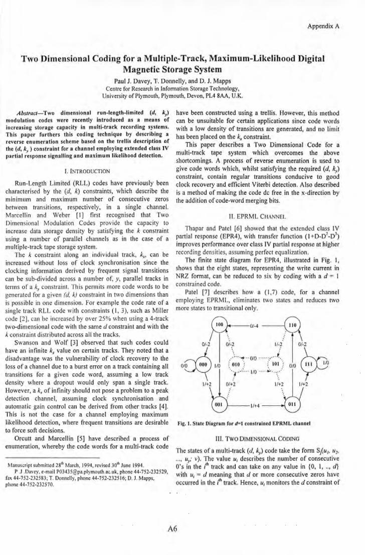
Appendix A

Two Dimensional Coding for a Multiple-Track, Maximum-Likelihood Digital Magnetic Storage System

Paul J. Davey, T. Donnelly, and D. J. Mapps Centre for Research in Information Storage Technology,

University of Plymouth, Plymouth, Devon, PL4 8AA, U.K.

Abstract-Two dimensional run-length-limited (d, k1)

modulation codes were recently introduced as a means of increasing storage capacity in multi-track recording systems. This paper furthers this coding technique by describing a reverse enumeration scheme based on the trellis description of the (d, k

1) constraint for a channel employing extended class IV

partial response signalling and maximum likelihood detection.

I. INTRODUCTION

Run-Length Limited (RLL) codes have previously been characterised by the (d, k) constraints, which describe the minimum and maximum number of consecutive zeros between transitions, respectively, in a single channel. Marce ll in and Weber [I] firs t recognised that Two Dimensional Modulation Codes provide the capacity to increase data storage density by satisfying the k constraint using a number of parallel channels as in the case of a multiple-track tape storage system.

The k constraint along an individual track, k., can be increased without loss of clock synchronisation since the clocking infonnation derived by frequent signal transitions can be sub-divided across a number of, y, parallel tracks in tenns of a ky constraint. This pem1its more code words to be generated for a given (d. k) constraint in two dimensions than is possible in one dimension. For example the code rate of a single track RLL code with constraints ( 1, 3), such as Miller code [2]. can be increased by over 25% when using a 4-track two-dimensional code with the same d constraint and with the k constraint distributed across all the tracks.

Swanson and Wolf (3] observed that such codes could have an infinite kx value on certain tracks. They noted that a disadvantage was the vulnerability of clock recovery to the loss of a channel due to a burst error on a track containing all transitions for a given code word, assuming a low track density where a dropout would only span a single track. However, a kx of infinity should not pose a problem to a peak detection channel, assuming clock synchronisation and automatic gain control can be derived from other tracks [4]. This is not the case for a channel employing maximum likelihood detection, where frequent transitions are desirable to force soft decisions.

Orcutt and Marcellin [5] have described a process of enumeration, whereby the code words for a multi-track code

Manuscript submitted 28th March, 1994, revised 30th June 1994. P .J .Davey, e-mail [email protected], phone 44-752-232529,

fa.'< 44-752-232583; T. Donnelly, phone 44-752-232516; D. J. Mapps, phone 44-752-232570.

have been constructed using a trellis. However, this method can be unsuitable for certain applications since code words with a low density of transitions are generated, and no limit has been placed on the kx constraint.

This paper describes a Two Dimensional Code for a multi-track tape system which overcomes the above shortcomings. A process of reverse enumeration is used to give code words which, whilst satisfying the required (d, ky) constraint, contain regular transitions conducive to good clock recovery and efficient Viterbi detection. Also described is a method of making the code de free in the x-direction by the addition of code-word merging bits.

11. EPRML CHANNEL

Thapar and Patel [6] showed that the extended class IV partial response (EPR4), with transfer function (I +D-D2 -D1

)

improves perfonnance over class IV partial response at higher recording densities, assuming perfect equalization.

The finite state diagram for EPR4, illustrated in Fig. I, shows that the eight states, representing the write current in NRZ fonnat, can be reduced to six by coding with a d = I constrained code.

Pate I [7] describes how a (I ,7) code, for a channel employing EPRML, eliminates two states and reduces two more states to transitional only.

0/-2

~~~ 1/+2

0/-2 1/-2

_)· ··""!'··· 010 ... ....... . i. .. ( 010 : ; tOt : ··:.r··: ... 1/0 .. .. . .:. . ... : __ ...

0/+2 1/+2

0/-2

00~ 1/+2

Fig. 1. State Diagram for d=l constrained EPRML channel

11 I. TwO DIMENSIONAL CODING

The states of a multi-track (d, ky) code take the fonn Sj(u1, u1,

... , ur· v). The value u1 describes the number of consecutive O's in the 1u. track and can take on any value in {0, I, .. , d} with u1 = d meaning that d or more consecutive zeros have occurred in the 1u. track. Hence, u1 monitors the d constraint of

A6

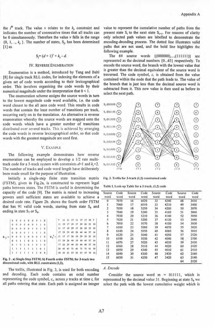
the ,~ track. The value v relates to the ky constraint and indicates the number of consecutive times that all tracks can be 0 simultaneously. Therefore the value v falls in the range {0, I, .. , ky } . The number of states, Sj, has been determined [I] as

IV. REVERSE ENUMERATION

Enumeration is a method, introduced by Tang and Bahl [8] for single track RLL codes, for indexing the elements of a given set of code words according to their lexicographical order. This involves organising the code words by their numerical magnitude under the interpretation that 0 < 1.

The enumeration scheme assigns the source words in turn to the lowest magnitude code word available, i.e . the code word closest to the all zero code word. This results in code words that contain the least number of transitions per track, occurring early on in the translation. An alternative is reverse enumeration whereby the source words are mapped onto the code words which have a greater number of transitions distributed over several tracks. This is ach ieved by arranging the code words in reverse lexicograph ical order, so that code words with the greatest magnitude are used first.

V. EXr\~tPLE

The following example demonstrates how reverse enumeration can be employed to develop a 1/2 rate multi­track code for a 3-track system with constraints d= I and ky=2. The number of tracks and code word length have deliberate ly been made small for the purpose of illustration.

Initially a single-step finite state transition matrix (FSTM), given in Fig.2a, is constructed to represent legal paths between states. The FSTM is useful in determining the capacity of the code [9]. The matrix is raised to increasing powers until sufficient states are available to achieve a desired code rate. Figure 2b. shows the fourth order FSTM that has 91 valid code words, starting from state Sa and ending in state S7 or Sa.

0 0 0 0 0 0 0 I 0 7 11 11 17 11 17 17 19 7

0 0 0 0 0 0 I I 0 11 19 17 29 17 29 26 )) 10

0 0 0 0 0 I 0 I 0 11 17 19 29 17 26 29 )) 10

0 0 0 0 I I I I 0 17 29 29 49 26 44 44 S1 14

B 3 • 0 0 0 I 0 0 0 I 0 B/ • 11 17 17 26 19 29 29 )) 10

0 0 I I 0 0 I I 0 17 29 26 44 29 49 44 S7 14

l: I 0 I 0 I 0 I 0 17 26 29 44 29 44 49 S1 14

I I I I I I 0 I 26 43 4) 71 4) 71 71 91 19

I I I I I I 0 0 19 )) J) S7 )) S7 S7 79 12

Fig. 2. a) Single-Step FSTJ\1; b) Fourth order FSTJ\1; for 3-track two dimensional code, with RLL constrainu (1,2),

The trellis, illustrated in Fig. 3, is used for both encoding and decoding. Each node contains an octal number representing the code symbol, c1, across y tracks at time t, for all paths entering that state. Each path is assigned an integer

Appendix A

value to represent the cumulative number of paths from the present state S1 to the next state S1• 1• For reasons of clarity only selected path values are labelled to demonstrate the encoding-decoding process. The dotted line illustrates valid paths that are not used, and the bold line highlights the following example.

The 64 source words {(000000), ... ,(111111)} are represented as the decimal numbers {0 ... 63} respectively. To encode the source word, the branch with the lowest value that is greater than the decimal equivalent of the source word is traversed. The code symbol, c, is obtained from the value contained within the node that the path leads to. The value of the branch that is just less than the decimal source word is subtracted from it. This new value is then used as before to select the next path.

s, (0.0.0;0) 0 0 s, (0.0,1;0) 0 s, (0.1.0;0) 0 SJ(O.I.I .O) 0 S, (1 ,0,0,0) 0

0 I = 0 I = I I • ]

Fig. 3. Trellis for 3-track (1 ,2) constrained code

Table I. Look-up Table for a 3 track, (1,2) rode

Source Code word word

0 7070 I 7060 2 7050 3 7040 4 7030 5 7020 6 7010 7 6160 8 6140 9 6120 10 6100 11 6070 12 6060 13 6050 14 6040 IS 6030

A. Encode

Source word

16 17 18 t9 20 2t 22 23 24 25 26 27 28 29 30 31

Code word 6020 6010 5250 5240 5210 5200 5070 5060 5050 5040 5030 5020 5010 4340 4300 4250

Source word

32 33 34 35 36 37 38 39 40 41 42 43 44 45 46 47

Code word

4240 4210 4200 4160 4140 4120 4100 4070 4060 4050 4040 4030 4020 4010 3430 3420

I = j

Source word 48 49 50 51 52 53 54 55 56 57 5& 59 60 61 62 63 64

0 0 0 0 0

I • 4

Code word

3410 3400 3070 3060 3050 3040 3030 3020 3010 2520 2500 2430 2420 24 10 2160 2140 2120

Consider the source word m = 011111 , which is represented by the decimal value 3 I. Beginning at state Sa we select the path with the lowest cumulative weight which is

A7

greater than the decimal equivalent of the source word. The path with weight 46 is the smallest value that is greater than 31, therefore we traverse this path to state S3• This state has a code symbol of 4 allocated to it, hence the first code symbol, c 1 of the code word is assigned the value 4. The path which has the greatest weight less than 31 is then subtracted from the decimal source word to give the new decimal source word. Hence 31-29 = 2. The process is then repeated, therefore the next path traversed has the weight 6, this leads to state S5 with value 2 which is assigned to c1. The new decimal source word is then calculated as 2-2 = 0. The process continues to state Sz., giving the third code symbol, c1

= 5, and ends in state S7 allotting the ftnal code symbol, c, =

0. Hence (0 11111) is encoded as

I 0 I 0 Cb Cz, c1, c, = 4 2 50= 0 I 0 0

0 0 I 0

B. Decode

To decode our example code word, (4250), sum the values on each of the branches that have the largest value below that of the branch taken. More simply, sum the values on each of the branches directly above the branch taken. Where there are no branches above the one traversed just add zero.

C. Substitlllion

As previously mentioned, code words with all transitions occurring on a single track are undesirable, since a burst error whilst reading that track would result in all timing information being lost. Therefore in our example we wish to prevent code word ( 4040) occurring. We achieve this by employing a substitution table, which prior to encoding, maps the source word onto another, arbitrary, unused source word that has a more desirable code word. The same table is used inversely after decoding to regenerate the original source word.

It can be seen from Table I that in the example code, code word ( 4040) is generated by decimal source word 42. Since only sixty four of the ninety one available code words are used, there are twenty seven remaining code words from which to chose a substitution. To maintain continuity, a replacement source word is chosen as 64 which gives a code word (2120).

VI. CHARGE CONSTRAINT

A null at de is desirable to match the spectral response of the magnetic recording channel. Therefore, to bound the accumulated charge, a charge control bit, P, can be added to each track between two adjacent code words. By monitoring the digital sum variation (DSV) of the two adjacent code words, the charge control bit is chosen to minimise the total DSV. To prevent the charge control bit violating the d constraint along each track, when a non-zero charge control

Appendix A

bit is adjacent to a non-zero code bit, the following substitutions have to be made.

OOOPO-+ valid for all P OOOPI-+ ifP=I substitute 00101 OIOPO-+ valid for all P 0 I OP I -+ if P= I substitute 00 I 00 lOO PO-+ valid for all P lOOP I-+ ifP=I substitute 10101

Making each track de-free has the added advantage of effectively introducing a k, constraint along each track. This is an important factor in determining the path memory of the Viterbi detector. The Viterbi detector requires non-zero samples to enable path merges, which result in decisions

VII. CONCLUSIONS

A Two Dimensional code has been described which is suitable for a multi-track tape system. The code words have been generated by reverse enumeration using a trellis. This technique produces code words which, whilst satisfying a given (d, ky) constraint, has a sufficient distribution of transitions to maintain detector clock synchronisation in the event of a severe dropout on any one of the tracks.

Where the encoding process results in code words that don't directly satisfy this latler requirement substitution code words are employed.

Additional charge control bits for each track improve the code's spectral properties and ensure frequent transitions to enable efficient Viterbi detection.

Alternatively, error correction information could be added to provide a degree of error control without any additional rate loss.

Vlll. REFERENCES

[I] Marcellin, M.W., & Weber, H.l., "Two Dimensional Modulation Codes", 1£££ J. Se/. Areas in Comms., Vot.IO, No.l, pp.2S4-66, January 1992.

[2] Miller, A., "Transmission System", US Patent3,108,261, October 1963. [3] Swanson, R.E., & Wolf, J.K., "A New Class of Two-Dimensional RLL

Recording Codes", 1£££ Tran.s. Magn., Vol.28, No.6, pp.3407-16, November 1992.

[4] Orcut~ E.K., & Marcellin, M.W., "Redundant Multitrack (d,k) Codes", 1£££ Trans.lnf 17reory, Vol.39, No.S, pp.I744-SO, September 1993.

[5] Orcutt, E.K., & Marcellin, M.W., "Enumerable Multitrack (d,k) Block Codes", 1£££ Tran.s. In/ 17reary, Vol.39, No.S, pp.l738-44, September 1993.

[6] Thapar, H.K., & Pate!, A.M., "A Class of Panial Response .System for Increasing Storage Density in Magnetic Recording", 1£££ Tran.s. Magn., Vol.23, No.S, pp.3666-68, September 1987.

[7] Pate!, A.M., "A New Digital Signal Processing Channel for Data Storage Products", 1£££ Traru. Magn., Vol.27, No.6, pp.4S79-84, November 1991.

[8] Tang, D., & Bahl, L., "Block Codes for a Class of Constrained Noiseless Channels", Information and Control, Vol.l7, pp.436-61, 1970.

[9] Siege!, P.H., "Recording Codes for Digital Magnetic Storage", 1£££ Trans. Magn., Voi.MAG-21, No.S, pp.l344-49, September 1985.

A8

I I i

SoftWare, written :in Pa~cal, f9t'tlle ]BM PC Corn pat~ble Host '' '

PROGRAM DIGITAL_COMPACT_CASSETIE_RECORDER (input,output); uses graph,crt,dos, consts,men u, fi lt,se I_ opt,export,disp lay, vi terbi;

{$1 convert.inc}

type linestring = string[80]; num_str =array [1..1000] of integer;

const PLAY= 0; REC =I; FF = 2; REW = 3; STOP= 4; TEST= 5; clock = $04; sync = $08; L_edge = $10; oversamp = $18; maxlen = 50 I; maxpass = 3; MAXTIME = 50000; clkmsk = $FB;

var GrDriver,GrMode:integer; option:char; CH:data_array; data:num_str; f: int_file;

Appendix B

{******······································································} Procedure TestGrMode; var Errcode: integer; begin

{GrDriver := Detect;} DetectGraph(GrDriver, GrMode); lnitGraph(GrDriver, GrMode, 'D:\TP\BGJ'); Errcode := GraphResult; CloseGraph; if Errcode <> grOK then writeln('Graphics Error: ',GraphErrorMsg(ErrCode));

end;

{*···········································································} Procedure Display _hex (var info:intege r); begin

convert_hex (info); write(' ');

end;

{***••••·····································································} Function Getdata(var data:integer) :boolean; var lopin :longint;

inp,val:byte; done :boolean;

begin lopin := 0; REPEAT

inp := PORT[P2C] AND $0 1; data := PORT[P2B] AND $OF; done := inp XOR val = I ; inc(lopin);

UNTIL done or (lopin > maxtime); vat := inp; getdata := done;

end;

{*···········································································} Function Get_DStr:boolean; var i:integer; begin

i:= l ;

82

Appendix B

while (getdata(data[i])) and (i < maxlen) do inc(i); if i=maxlen then Get_DStr :=true else Get_DStr := false;

end;

{*···········································································} Procedure Viewdata; var i:integer; begin

repeat fori := I to maxlen do data[i] := port[plb] and $Of; for i:= I to maxlen do Display_hex(data[i]); until keypressed = true;

end;

{·············································································} Procedure Getdval(var v:real; i:integer); const testdata:ARRA Y [ 1 .. 15] OF REAL= (0.8,-0.3,0.8,0.3,-0.1 ,- 1 ,-0.5,0.8,-0.3,0.8,0.3,-0.1 ,-l ,-0.5,0); var r:integer; begin

{r:= Random( l024); v:= (r-5 12)/512;} v:= testdata[i];

end;

{············································································} Procedure ANALOG_DISPLA Y; const teste I :tilt_ array = (-0.2,-0.9, I ,-0.3,-0.2);

testc2:fi lt_array = (-0.1 ,-0.3 , I ,-0.9,0.2); testc3:filt_array = (-0. 1,-0.9,1,-0.3,0.2); testc4:fi lt_array = (-0.5,0, I ,0,-0.5);

var coeff: filt_array; width,s lim:real; x,y,offset:integer; f: int_fil e; rl ,r2 : text;

begin if FileExists(f,'c:\pjd\dccr\SAMPLES2.DA T') then Reset( f) else Rewrite(t); ln itGraph(GrDriver,GrMode,'d:\tp\bgi'); SetBkcolor (black); repeat

for x:= I to 4 do for y := I to 2048 do read(f,Ch[x,y]); { filt_3tap( 4, I);} {auto_ equalize( 4,2,coeft);} filt_prog(CH,4,5,testc2); {slim := get_pw50(2);}

until eof(f) OR Display_Data(Ch,4,5,-l, I,IOO,false,O); CloseGraph; close( f);

end;

{············································································} Procedure Save_Sig(var Sigsave:boolean); var sigfi le:string;

done: boo lean; begin

done := false; WTNDOW( I4, l0,65,11 ); TEXTBACKGROUND(RED); clrscr; Sigsave:=false; done:=false;

83

write('Do you want to save the readback signals <y/n>? '); if getyn then repeat

write('Enter filename to store signals '); readln(sigfile); if(Length(sigfile) > 12) OR (Length(sigfile) < I) then begin

clrscr; write('lnvalid filename!! Do want to try again <y/n>? '); if not getyn then done:=true;

end else if FileExists(f,sigfile) then begin

clrscr; write(sigfile,' already exists do you want to overwrite <y/n> '); if getyn then begin

Sigsave := true; Reset( f) ;

end; end else begin

Sigsave:=true; Rewrite( f) ;

end; until done or Sigsave: WINDOW( I, I ,80,24); TEXTBACKG ROUND(BLACK);

Appendix B

end; {············································································} Procedure Play_ Tape; var y,x: integer;

Sigsave:boolean;

begin Save_Sig(Sigsave); Out_Port(PLA Y); lni tGraph(GrDriver,GrMode,'D:\TP\BGJ'); SetBkcolor (black); DELAY( I 000); {I SECOND DELAY} for y := I to 2048 do for x := I to 4 do IN_PORT(Ch[x,y)); REPEAT

for y := I to 2048 do for x := I to 4 do IN_PORT{Ch[x,y]); Plot_ Data (eh, I ,4,0, I, I OO,false,O); if Sigsave then

for x:= I to 4 do for y := I to 2048 do write(f,Ch[x,y]); UNTIL KEYPRESSED AND (Ord(READKEY)=ESC); RESET_SYS; CLOSEGRAPH; if Sigsave then Close( f); {crap := readkey;}

end;

{············································································} PROCEDURE WR1TE_TAPE; var i:integer; begin

OUT _PORT(REC); OUT _PORT(Hi(PERIOD)); OUT _PORT(Lo(PERIOD)); OUT _PORT(CODE); OUT _PORT(D _Type); ifD_TYPE = SEQ THEN begin

{send high byte} {send low byte}

84

OUT_PORT (SEQLEN-1); fori := I to seqlen do OUT_PORT(seqval[i]);

end; clrscr; InitGraph(GrDriver,GrMode,'d:\tp\bgi'); SetBkcolor (Red); Setcolor (Yellow); SetTextStyle(SansSerifFont, HorizDi.r, 8); OutTextXY (120,180, 'RECORDING!'); SetTextStyle(Defau ltfont,HorizDir, I); Outtextxy (140,440, 'Hit ESC to Terminate and return to main menu'); while ord(upcase(READKEY)) <> ESC do write(CHR(bell)); close graph; reset_sys;

end;

{$1 TESTS.INC}

Appendix 8

{******************••························································}

begin TestGrMode; port[P2CTRL] := $83 ; port[P2CTRL] :=$OF; RESET_SYS;

{SET P2A=O/P P28=1/P P2C=O/P,I/P} {SET BUSY HIGH}

repeat Display_Menu (Main_Menu); Get_Menu_Response (Main_Menu, option); case option of

'S': reset_sys; 'R': OUT_PORT (REW); 'F': OUT_PORT (FF); 'W': WRITE_TAPE; 'P': PLAY _TAPE; 'T': Test_Se l; 'V': viterbi_det(ch,200,5,6); 'D': ANALOG_DISPLA Y; '0': SEL_OPTION;

end; until ord(option) = ESC; clrscr; halt;

end.

{*···········································································}

BS

unit consts; interface const maxlen = 50;

type data_array =array (1..8, 1..2048] of integer; datarray = array [ l .. maxlen] of integer;

const maxdata = 2048;

BELL =7; CR = 13; ESC = 27; SPACE = 32; R_ARROW = 77; L_ARROW = 75; D_ARROW = 80; U_ARROW = 72;

PIA= $300; PIB = $301; PlC= $302; P ICTRL = $303; P2A = $304; P2B = $305; P2C = $306; P2CTRL = $307;

implementation end.

B6

Appendix B

unit Codes; interface uses consts; type

seqarray = array [0 .. 1 00] of byte; const

datend = 40; Procedure Miller_ Squared_ Encoder(var M2:seqarray; data:seqarray); Procedure Miller_ Squared_ Decoder(var data:seqarray; M2:seqarray);

implementation

Procedure Miller_ Squared_ Encoder(var M2:seqarray; data:seqarray); type stat_ val = (A,B,C,D,E,F,G,H,J,J); var M2state : stat_ val;

ii:integer; begin

M2state := C; for ii := 0 to datend do case M2state of

A: begin if data[ii) = 0 then M2state := B else M2state := I; M2[2*ii) := I; M2[2*ii+IJ := 0;

end; 8: begin

if data[ii) = 0 then M2state := D else M2state := C; M2[2*ii] := 0; M2[2*ii+l] := 0;

end; C: begin

if data[ii] = 0 then M2state := D else M2state := E; M2(2*ii] := 0; M2(2*ii+ l) := I;

end; 0 : begin

if data[ii] = 0 then M2state := A else M2state := B; M2[2* ii] := I; M2[2*1+1] := I;

end; E: begin

if data[ii] = 0 then M2state := F else M2state := C; M2[2*ii] := I; M2(2*ii+l] := 0;

end; F: begin

if data[ii] = 0 then M2state := H else M2state := G; M2[2*ii] := 0; M2(2*ii+I] := 0;

end; G: begin

if data[ii] = 0 then M2state := H else M2state := J; M2(2*ii] := 0; M2(2*ii+I] :=I;

end; H: begin

if data[ii] = 0 then M2state := F else M2state := E; M2[2*ii] := I; M2[2*ii+ I] := I;

end;

87

Appendix B

I : begin if data[ii] = 0 then M2state := F else M2state :=A; M2[2*ii] := 0; ifdata[ii] = 0 then M2[2*ii+ J] := 0 else M2[2*ii+l] := 1;

end; J: begin

if data[ii] = 0 then M2state := D else M2state := G;

M2[2*ii] :=I; ifdata[i i] = 0 then M2[2*ii+l] :=I else M2[2*ii+l] := 0;

end; end;

end;

Procedure Miller _Squared_Decoder(var data:seqarray; M2:seqarray); var ii :integer; begin

for ii := I to datend do data[ii] := (M2[2*ii] and M2[2*ii+ l] and not M2[2*ii+3])

or (not M2[2*ii] and not M2[2*ii+ I] and M2[2*ii+3]);

end;

end.

88

Appendix B

unit display;

interface uses consts,graph,crt; Procedure Plot_ Data (var Data: data_ array; ChSt,ChEnd:integer;sclY ,xscl:real;

xoffset:integer; axis:boolean; sample:integer); Procedure Scope (var data:data_array; ChSt,ChEnd:integer;sclY,xscl:real;

xoffset:integer); Function Display_ Data(var Data:data _array; ChSt,ChEnd:integer;sclY ,zoom:real;

offset: integer; axis:boolean; sample:integer):boolean;

implementation

Procedure Plot_ Data (var Data: data _array; ChSt,ChEnd:integer;sciY,xscl:real; xoffset:integer; axis:boolean; sample: integer);

var maxy,miny : real ; x,y,ysize,yoffset,Xmax,Xlim,yaxis,sampt,ysamp :integer; yscl:real;

begin clearviewport; Ysize := round((GetMaxY -1 0)/(Chend-ChSt+ I)); Xmax:= GetMaxX; Xlim:= Round(Xmax/Xscl); for y := ChSt to ChEnd do begin

maxy := DATA[y,l +xoffset]; miny := DATA[y,l+xoffset]; for x := xoffset+2 to xoffset+Xlim do

if DATA[y,x] > maxy then maxy := DATA[y,x] else if DATA[y,x] < miny then miny := DATA[y,x] ;

if sclY = -1 then begin yscl := Ysize I (maxy- miny + I); yoffset := Round(((y-ChSt)* Ysize)-(m iny*yscl));

end else if sciY = 0 then begin

yscl := Ysize / 256; yoffset := Round((y-ChSt)*Ysize);

end else begin

yscl := sciY; yoffset := Round(((y-ChSt)*Ysize)-(miny*yscl));

end; ifXmax > (2048-xoffset)*xscl then xoffset := 2047-XIim; yaxis := round((ysize*(y-chst+ I ))-ysize/2); if axis then begin

setcolor(Lightgray); line (O,yaxis,xmax,yaxis);

end;

SetColor(black+y); moveto (O,round((DA T A[y ,xoffseWyscl)+yoffset)); X:= I; repeat

lineto(round((x-1 )*xscl),round((DA T A[y,x+xoffset]•yscl)+yoffset)); inc(x);

until (round((x-1 )*xscl) >= Xmax) or (x > maxdata);

if sample > 0 then begin

sampt := 0;

89

Appendix B

setcolor(yellow); repeat

ysamp := round((Data[y,sampt+xoffseWyscl)+yoffset); line(round((sampt-1 )• xscl),yaxis,round((sampt-1 )• xscl),ysamp ); sampt := sampt + sample;

until (round(sampt•xscl) >= Xmax) or (sampt > maxdata); end;

end; end;

Appendix B

{············································································} Procedure Scope (var data:data_array; ChSt,ChEnd:integer;sciY,xscl:real;

xoffset: integer); var maxy,yoffset,ysize,yp I ,yp2,yp3 :longint;

x,y,xp I ,xp2,Xmax :integer; yscl:array [1..4) ofreal; m iny:array [ 1..4] of longint;

begin clearviewport; Y size := round(GetMaxy-1 0/(ChEnd-ChSt+ I)); Xmax:=GetMaxX; for y := ChSt to ChEnd do begin

maxy := DATA[y, l] ; miny[y] := DATA[y,l]; for x := 2 to maxdata do

ifDATA[y,x] > maxy then maxy := DATA[y,x] else if DATA[y,x] < miny[y] then miny[y] := DATA[y,x];

if sclY =-I then yscl[y] := Ysize I (maxy- miny[y] + I) else if sclY = 0 then yscl[y] := Ysize / 256 else yscl[y] := sciY;

end; repeat

if Xmax > (2048-xoffset)*xscl then xoffset := 204 7-Round(Xmax/xscl); X:= I ; repeat

for y:= chst to chend do begin

setcolor (black); yoffset := (y-ChSt)*Y size- I; xp I := Round((x-1 )*xscl); xp2 := Round(x*xscl); yp I := ysize-Round((Data[y,x- 1 +xoffset]-miny[y])*yscl[y])+yoffset; yp2 := ysize-Round((Data[y ,x+xoffset)-m iny[y ])* yscl[y ])+yoffset; yp3 := ysize-Round((Data[y,x+ I +xoffset]-miny[y])*yscl[y])+yoffset; line (xpl,ypl,xp2,yp2); setcolor (black+y); line (xpl,yp2,xp2,yp3);

end; inc(x);

until (round((x- 1 )*xscl) >= Xmax) or (x > maxdata); xoffset := xoffset + I ; until xmax > (2048-xoffset)•xscl;

end;

{············································································} Function Display_ Data(var Data: data_ array; ChSt,ChEnd:integer;sclY ,zoom:real;

offset:integer; axis:boolean; sample:integer):boolean; var

fin,valid:boolean; resp:char;

810

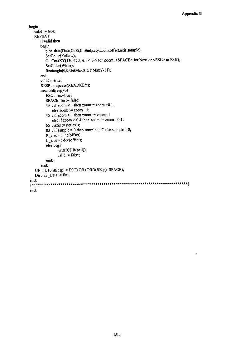
begin valid :=true; REPEAT

if valid then begin

plot_ data(Data, ChSt, Ch End,sc ly ,zoom ,offset,ax i s,sam pie); SetColor(Yellow); OutTextXY(I30,470,'Hit <+/->for Zoom, <SPACE> for Next or <ESC> to Exit'); SetColor(White); Rectangle(O,O,GetMaxX,GetMaxY -!I);

end; valid := true; RESP := upcase(READKEY); case ord(resp) of

ESC : fin:=true; SPACE: fin :=false; 43 :if zoom< I then zoom:= zoom +0.1

else zoom :=zoom+ I; 45 : if zoom > I then zoom := zoom -I

else if zoom > 0.4 then zoom := zoom - 0.1; 65 : axis := not axis; 83 : if sample= 0 then sample:= 7 else sample :=0; R_arrow: inc(offset); L _arrow : dec( offset); else begin

end; end;

write(CHR(bell)); valid :=false;

UNTIL (ord(resp) = ESC) OR (ORD(REsp)=SPACE); Display_Data :=fin;

Appendix B

end;

{***••·······································································} end.

Bll

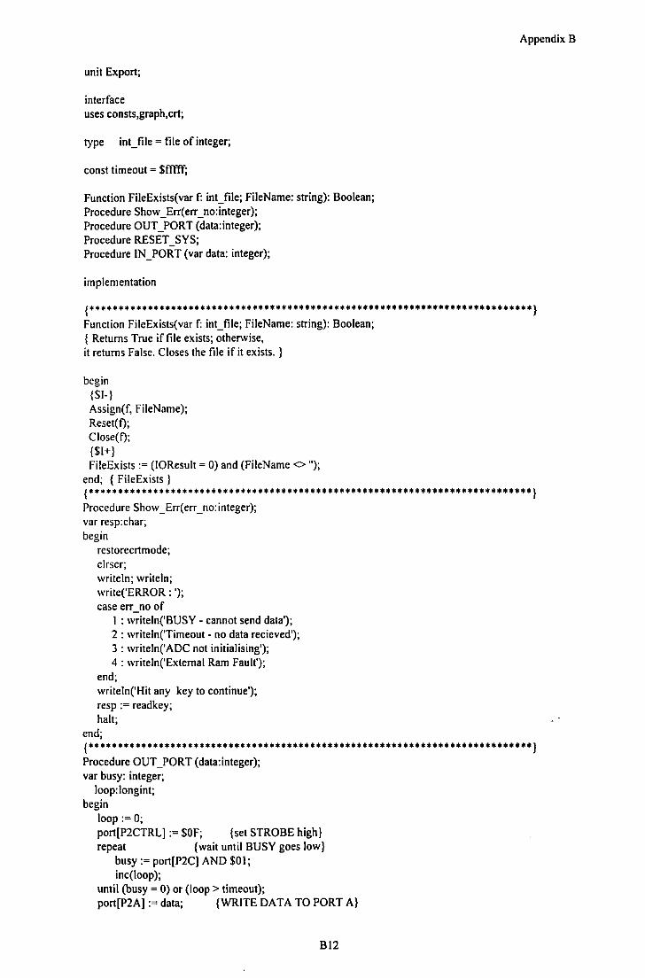
unit Export;

interface uses consts,graph,crt;

type int_file =file of integer;

cons! timeout = $fffff;

Function FileExists(var f: int_file; FileName: string): Boolean; Procedure Show_ Err( err_ no: integer); Procedure OUT_PORT (data: integer); Procedure RESET_SYS; Procedure IN_PORT (var data: integer);

implementation

Appendix B

{**•·······································································••) Function FileExists(var f: int_file; FileName: string): Boolean; { Returns True if file exists; otherwise, it returns False. Closes the file if it exists. }

begin {SI-} Assign(f, FileName); Reset( f); Close( f); {$1+} FileExists := (IOResult = 0) and (FileName <> ");

end; { FileExists }

{············································································} Procedure Show _Err(err_no:integer); var resp:char; begin

restorecrtmode; clrscr; writeln; writeln; write('ERROR : '); case err no of

I : writeln('BUSY- cannot send data'); 2 : writeln('Timeout - no data recieved'); 3 : writeln('ADC not initialising'); 4 : writeln('External Ram Fault');

end; writeln('Hit any key to continue'); resp := readkey; halt;

end;

{*···········································································} Procedure OUT _pORT (data: integer); var busy: integer;

loop: longint; begin

loop:= 0; port[P2CTRL] :=$OF; {set STROBE high} repeat {wait until BUSY goes low}

busy:= port[P2C) AND $01; inc(loop);

until (busy = 0) or (loop> timeout); port[P2A) :=data; {WRITE DATA TO PORT A}

Bl2

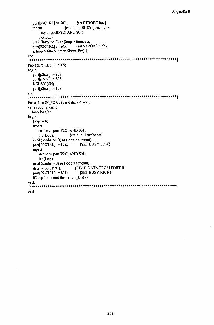
Appendix B

port[P2CTRL) := $0E; {set STROBE low} repeat {wait until BUSY goes high}

busy := port(P2C] AND $0 I; inc(loop);

until (busy <> 0) or (loop > timeout); port(P2CTRL] :=$OF; {set STROBE high} if loop> timeout then Show_Err(l);

end;

{*···········································································} Procedure RESET_SYS; begin

port[p2ctrl] := $09; port[p2ctrl) := $08; DELAY (50); port[p2ctrl) := $09;

end;

(••••······································································••) Procedure IN_PORT (var data: integer); var strobe: integer;

loop:longint; begin

loop:= 0; repeat

strobe:= port(P2C) AND SOl; inc(loop); {wait until strobe set}

·until (strobe<> 0) or (loop> timeout); port[P2CTRL] := $0E; {SET BUSY LOW} repeat

strobe:= port(P2C) AND $01; inc(loop);

until (strobe= 0) or (loop> timeout); data:= port[P2B); {READ DATA FROM PORT B) port[P2CTRL) :=$OF; {SET BUSY HIGH} if loop> timeout then Show_Err(2);

end;

(*••••·······································································} end.

Bl3

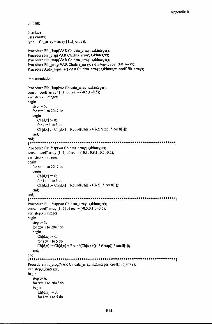
unit lilt;

interface uses consts; type lilt_ array= array [1..5] of real;

Procedure Filt_3tap(VAR Ch:data_array; s,d:integer); Procedure Fir_5tap(VAR Ch:data_array; s,d:integer); Procedure Filt_5tap(VAR Ch:data_array; s,d:integer); Procedure Filt_prog(VAR Ch:data_array; s,d:integer; coeff:filt_array); Procedure Auto_Equalize(VAR Ch:data_array; s,d:integer; coeff:filt_array);

implementation

Procedure Filt_3tap(var Ch:data_array; s,d:integer); const coeff:array [1..3] of real= (-0.5,1,-0.5); var step,x,i:integer; begin

step:= 6; for x:= I to 204 7 do begin

Ch[d,x] := 0; for i := I to 3 do Ch[d,x] := Ch[d,x] + Round(Ch[s,x+{i-2)*step] • coeff[i]);

end; end;

Appendix B

{**•·········································································} Procedure Fir_5tap(var Ch:data_array; s,d:integer); const coeff:array [ 1..5] of real = ( -0.1 ,-0.9, I ,-0.3,-0.2); var step,x,i:integer; begin

for x:= I to 204 7 do begin

Ch[d,x] := 0; for i := I to 3 do Ch[d,x] := Ch(d,x] + Round(Ch[s,x+{i-2)] • coeff[i]);

end; end; , .•.......•..•.......••.........•......••••••..•....••••••••••••••••.•..••••• } Procedure Filt_5tap(var Ch:data_array; s,d:integer); const coeff:array [ 1 .. 5] of real = ( -0.5,0, I ,0,-0.5); var step,x,i:integer; begin

step:= 3; for x:= I to 2047 do begin

Ch[d,x] := 0; for i := I to 5 do Ch[d,x] := Ch[d,x] + Round(Ch[s,x+((i-3)*step)] • coeffl:i]);

end; end; , ............................................................................ } Procedure Filt_prog(VAR Ch:data_array; s,d:integer; coeff:filt_array); var step,x,i:integer; begin

step:= 6; for x:= I to 2047 do begin

Ch[d,x] := 0; for i := I to 5 do

814

end; end;

Ch[d,x] := Ch(d,x] + Round(Ch[s,x+(i-3)*step] • coeff[i]);

Appendix B

{**•·········································································} Procedure Auto_Equalize(var Ch:data_array; s,d:integer; coeff:filt_array); var step,x,i:integer; begin

coeffll] := -0.5; coeffl2] := 0; coeff[3] := I; coeff[4] := 0; coeffl5] := -0.5;

step:= 6; for x:= 13 to 17 do begin

Ch[d,x] := 0; for i := I to 5 do Ch[d,x] := Ch[d,x] + Round(Ch[s,x+(i-3)*step]• coeff[i]);

end; for x:= I 8 to 2000 do begin

Ch[d,x] := 0; for i := I to 5 do coef!Ii] := coeffli]+(0.0003*(Ch[s,x-i]-Ch[d,x-i])); for i := I to 5 do Ch[d,x] := Ch[d,x] + Round(Ch[s,x+(i-3)*step] • coef!Ii]);

end; end;

{············································································} end.

815

I

r'

((c ~ND1$(=6)lOR(c AJ'JEi $f=2)!0R(c:AND $fc=4):0R (c.AND Sf=S))ihen begiii

if.c~AND!$040000 <>iOiihenlinc(bcnt);: inc(couni); , write( count,' '); bin2hex( c); writeln(g;' :);

end; ·end; · writeln(g,'bitcount= ';belli); close(gj;

'end;

:begin ;Code!_2l);

end!

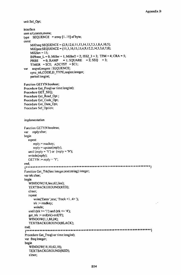
unit Sei_Opt;

interface uses crt,consts,menu; type SEQUENCE =array [1..15] ofbyte;

const Mil2seq:SEQUENCE = (2,9,12,6,11,13,14,15,7,3,1,8,4,10,5); Mil2pos:SEQUENCE = (11,1,10,13,15,4,9,12,2,14,5,3,6,7,8);

Mil21en = 15; BiPhase_L = 0; Miller= I; Miller2 = 2; ISS2_3 = 3; TPM = 4; CRA = 5; PRBS = 0; RAMP = I; SQUARE = 2; SEQ = 3; TIMER = $CO; ADCTST = $C I;

var seqval,seqpos : SEQUENCE; sync_ trk,CODE,D _ TYPE,seqlen:integer; period:longint;

Function GETYN:boolean; Procedure Get_Freq(var time:longint); Procedure GET_ SEQ; Procedure Get_ Read_ Opt ; Procedure Get_ Code_ Opt; Procedure Get_ Data_ Opt; Procedure Se I_ Option;

implementation

Function GETYN:boolean; var reply:char; begin

repeat reply:= readkey; reply:= upcase(reply);

until (reply= 'Y') or (reply= 'N'); writeln(reply); GETYN :=reply= 'Y';

end;

Appendix B

t•···········································································} Function Get_ Trk(line:integer;text:string):integer; var trk:char; begin

WINDOW(l8,line,62,1ine); TEXTBACKGROUND(RED); clrscr; repeat

write('Enter ',text,' Track <1 . .4> '); trk := readkey; write In;

until (trk >= 'I') and (trk <= '4'); get_trk := ord(trk)-ord('O'); WINDOW( I, I ,80,24); TEXTBACKGROUND(BLACK);

end;

t•···········································································} Procedure Get_Freq(var time:longint); var freq:integer; begin

WINDOW(IS, I 0,62, I 0); TEXTBACKGROUND(RED); clrscr;

834

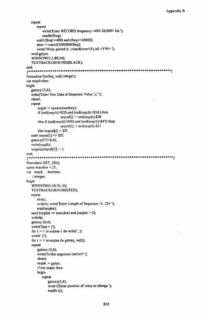
repeat repeat

write('Enter RECORD,frequency <400-20;000> Hz '); readln(freq);

until (freq>=400) and (freq<=20000); time := round(5000000/freq); write('Write period is ',round(time/IO),'uS <Y/N> ');

until:getyn; WINDOW( I, I ,80;24); TEXTBACKGROUND(BLACK);

Appendix B

end;

(•············~~·~··~··································~·~········~··········} Procedure GetSeq_ val(i:integer); vilr seqch:char; begin

gotoxy (5,6); wdte('Enter Hex Data at Sequence Value ',i,' '); clreoi; repeat

seqch := upcase(readkey); if (ord(seqch)>$21) and (ord(seqch)<$3A) then

seqval[i] := ord(seqch)c$30 else if (ord(seqch)>S40) and (ord(seqch)<$47),ihell

seqval[i] := ord(seqch)-$37 else seqval[i] := $ff;

Lintil seqval[i] <> $ff; gotoxy(i • 2+6,4 ); write(seqch); seqpos[seqval[i]l := i;

end; .

(••··········~································································} Procedure GET_SEQ; const maxsle11 = 32; var seqok : boolean;

!:integer; begin

WINDOW(4,10,76,16); liEXTBACKGROUND(RED); repeat

clrscr; write In; write('Enier Lengih of Sequence <1 .. 32> '); read(seqlen);

until (seqlen <= maxsle11) 11ncl (seqlen > 0); write In; gotoxy (0,4); write('Seq = {'); for i := I to seqlen-1 do write(' ,'); write(' } '); fori:= I to·seqlelt do getseq_ val(i); repeat

goioxy (5,6); write('Js;this sequence: correct?'); clreol; · seqok :.= getyn; ifnot seqokthen begin

repeat gotoxy(5,6); write ('~nter position of value,to change'); read In (i);

835

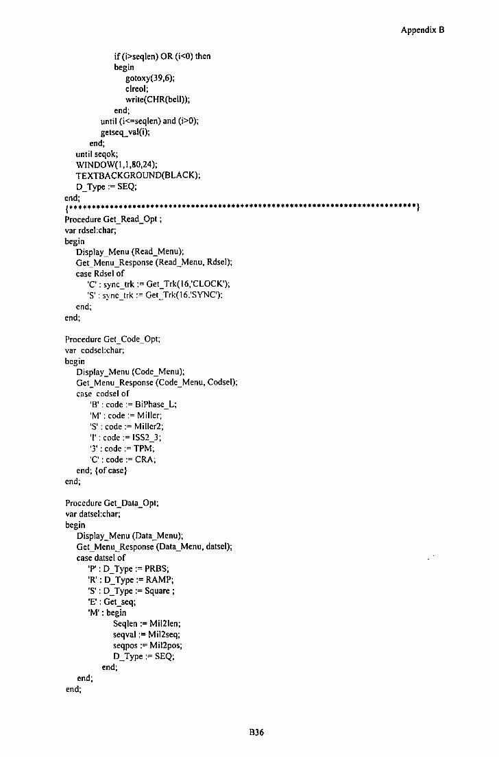
if (i>seqlen) OR (i<O) then begin

gotoxy(39,6); clreol; write(CHR(bell));

end; until (i<=seqlen) and (i>O); getseq_ val(i);

end; until seqok; WINDOW( 1,1,80,24); TEXTBACKGROUND(BLACK); D _Type := SEQ;

end;

Appendix B

t·············································································} Procedure Get_ Read_ Opt ; var rdsel:char; begin

Display_Menu (Read_Menu); Get_Menu_Response (Read_Menu, Rdsel); case Rdsel of

'C' : sync_trk :=Get_ Trk( 16,'CLOCK'); 'S': sync_trk := Get_Trk(I6.'SYNC');

end; end;

Procedure Get_ Code_ Opt; var codsel:char; begin

Display_Menu (Code_Menu); Get_Menu_Response (Code_Menu, Codsel); case codsel of

'B': code:= BiPhase_L; 'M': code:= Miller; 'S' : code := Miller2; 'I': code:= 1SS2_3; '3' :code := TPM; 'C' : code := CRA;

end; {of case} end;

Procedure Get_Data_Opt; var datsel:char; begin

Display_ Menu (Data_Menu); Get_Menu_Response (Data_Menu, datsel); case datsel of

'P': D_Type := PRBS; 'R' : D _Type := RAMP; 'S': D_Type :=Square; 'E' : Get_seq; 'M': begin

end; end;

Seqlen := Mi12len; seqval := Mil2seq; seqpos := Mil2pos; D_Type := SEQ;

end;

B36

Procedure Se I_ Option; var opt: char; begin

repeat Display_ Menu (Options_Menu); Get_Menu_Response (Options_Menu, opt); case opt of

'R': Get_Read_Opt; 'C': Get_Code_Opt; 'F' : Get_Freq(period); 'D': Get_Data_Opt;

end; until ord(opt) = Esc;

end;

end. unit Viterbi;

interface

uses consts,graph,crt; Procedure Precode(var data:data_array; dlen,din,dout:integer); Procedure Man_ decode(var data: data_ array; dlen,din,dout:integer); Procedure Viterbi_ Det(var data:data _array; vlen, vin, vout:integer); Procedure Detector(ch:data _array; s,d:INTEGER); Procedure Detector2(ch:data_array; s,d:INTEGER); Function Peak(var s,x:integer; Ch:data_array):integer; Function Get_PWSO(ch:data_array; s:integer):real;

implementation

Appendix B

{*···········································································} Procedure Precode(var data:data _array; dlen,din,dout: integer); var i:integer; begin

for i := I to dlen do data[dout, i] := (data[din, i] XOR data[dout, i-1]) AND $01;

end;

{············································································} Procedure Man_decode(var data:data_array; dlen,din,dout:integer); var i:integer; begin

fori := I to (dlen div 2) do data[dout, i] :=data[ din, i0 2];

end;

t············································································) Procedure Viterbi_Det(var data:data_array; vlen,vin,vout:integer); var f,i,z :integer; n,o,p,a,b,c,d,v :real; State I ,StateO : array [ 1..400] of longint; Wp,Wn: array [1..100) of real;

begin clrscr; f:=O; fori := I to vlen do begin

data[vout,i] :=-I; {initialise output value} v := data[ vin, I OO+(i'7)]11 0;

B37

Wp[l] := 0; Wn[l] := 0; n:= Sqr(v-1); o:= Sqr(v); p:= Sqr(v+l); a:= Wp[i] + o; b:= Wn[i] + n; c:= Wn[i] + o; d:= Wp[i] + p;

if a> b then begin

Wp[i+l] := b; State I [i] := I;

end else begin

Wp[i+l] :=a; State I [i] := 0;

end;

ifc > d then begin

Wn[i+l] := d; StateO[i] := I;

end else begin

Wn[i+ I] := c; StateO[i] := 0;

end;

while (Wp[i+l)> I) AND (Wn[i+l)>l) do begin

Wp[i+ I] := Wp[i+ I) -I; Wn[i+l] := Wn[i+l]-1

end;

if (b >a) AND (c >d) then begin

for z := fto i-1 do data[vout,z) := Statel[z]; {PrevStatel} f:=i;

end else if(a >b) AND (d >c) then begin

for z:= fto i-1 do data[vout,z] := StateO[z]; {PrevStateO} f:=i;

end; write(v:8:3);

end; write In; fori:= I to vlen do write(data[vout,i]:3); write In; precode(data, vlen, vout, vout+ I); fori:= I to vlen do write(data[vout+l,i]:3); write In; man _decode(data,vlen,vout+ I ,vout+2); for i := I to (vlen div 2) do write(data[vout+2,i):3); writeln; write('Hit <ENTER> to continue'); read In;

end;

Appendix B

{············································································} Function Peak(var s,x:integer; Ch:data_array):integer; var count : integer; begin

count:= 0;

838

while Ch[s,x] = Ch[s,x+ I] do inc(x); ifCh[s,x] > Ch[s,x+l] then repeat

inc(x); ifCh[s,x] = Ch[s,x+l]then inc(count);

until (Ch[s,x] < Ch[s,x+l]) and (Ch[s,x+l] < Ch[s,x+2]) else if Ch[s,x] < Ch[s,x+ I] then repeat

inc(x); ifCh[s,x] = Ch[s,x+l] then inc(count);

until (Ch[s,x] > Ch[s,x+l]) and (Ch[s,x+l] > Ch[s,x+2]); Peak:= round(x-(count/2));

end;

Appendix B

{*···········································································} Function Get_PW50(ch: data_array; s:integer):real; var cnt,pk I ,pk2,xl ,x2,pulse_no,x:integer;

ph50,pw50,total,a I ,a2,m I ,m2 :real;

begin pulse_no := 0; total:=O; x:=IOO; pk I := peak(s,x,ch); repeat

pk2 := peak(s,x,ch); ph 50 := Ch[s,pk I] - (Ch[s,pk 1]-Ch[s,pk2])/4; cnt :=I; ifCh[s,pkl] > ph50 then begin

while Ch[s,pk l-ent]> ph 50 do inc(cnt); xl := pkl-cnt; cnt:=l; while Ch[s,pk I +cnt] >ph 50 do inc(cnt); x2 := pk I +cnt;

end else begin

while Ch[s,pk l-ent] <ph 50 do inc(cnt); xl := pkl-cnt; cnt:=l; while Ch[s,pk I +en!] <ph 50 do inc(cnt); x2 := pkl+cnt;

end; m2 := Ch[s,x2]-Ch[s,x2-l]; ifm2 = 0 then a2 := 0 else a2 := (ph50-Ch[s,x2])/m2; ml := (Ch[s,xl]-Ch[s,xl+l]); ifml =Othenal :=0 else a2 := (ph50-Ch[s,x I ])/m I; pw50 := (a2+x2)-(al+xl); total := total + pw50; inc(pulse_no); writeln(pkl :5, Ph50, xI :5, x2:5, pw50);

pkl := pk2; until pk I > 2000; writeln(total/pulse _no);

Get__pw50 := total/pulse_no; end;

{*···········································································} Procedure Detector2(ch:data _array; s,d:INTEGER); var same,x,i:integer; begin

B39

same:=O; for x:= I to 2047 do begin

if (Ch[s,x+ I ]-Ch[s,x]) > 0 then begin

if (Ch(s,x]-Ch[s,x-4]) >= 0 then Ch[d,x] := $FF else Ch[d,x] := 0;

end else if(Ch[s,x+ 1]-Ch[s,x]) < 0 then begin

if (Ch[s,x]-Ch(s,x-4]) <= 0 then Ch[d,x] := 0 else Ch[d,x] := $FF;

end; if(Ch[s,x+l]-Ch[s,x]) = 0 then begin

inc(same); Ch[d,x] := Ch(d,x-1];

end else if same> 0 then begin

fori:= I to round(same/2) do Ch[d,x-i]:=Ch[d,x]; same:= 0;

end; end;

end;

Appendix B

{**••········································································} Procedure Detector(ch:data_array; s,d:INTEGER); var x:integer; begin

for x:= I to 2047 do begin

if (Ch[s,x+ 1]-Ch(s,x)) > 0 then Ch[d,x] := $FF else if(Ch[s,x+I]-Ch[s,x]) < 0 then Ch(d,x] := 0 else if(Ch[s,x+I]-Ch[s,x]) = 0 then Ch(d,x] := Ch[d,x-1];

end; end; end.

840

I . . t,.

.AppendixC . ~ -· .

SoftWare; w.ritten' in lfMS320C25 Assembly Langua·ge, for .the

IDigitali Compact,Cassette Tape Recording System.

1Cl

Appendix C

TMS32025/

;u+ THIS PROGRAM WAS DEVELOPED BY P. DA VEY WRITTEN IN TMS32025 ASSEMBLEY ;**+ CODE IT CONTROLS THE READING & WRITING OF DIGITAL OAT A ON TAPE

TITLE "MULTI CHANNEL DIGITAL CASSETTE TAPE OAT A RECORDER"

TEXAS

EXTERN _BackChannei,TSTBCHSND,TSTBCHGET •••••••••••••••••••••••••••••••••••••••••••••••••••••••••••••••••••••••••••••• . ···- MEMORY MAP . .BLKO EQU >200 .BLKI EQU >300 .BLK2 EQU >0060 .XRAM EQU >8000

.PROM EQU >8000

.ADC I EQU >2000

.ADC2 EQU >2001

.ADC3 EQU >2002

.ADC4 EQU >2003

.WRITEEQU >2000

;PORTS PARPORT EQU CONPORT EQU

0 I

;INTERNAL RAM >200 - >300 ;INTERNAL RAM >300 - >400 ;INTERNAL RAM >060- >07F ;EXTERNAL RAM >8000 - >9FFF

;FAST PROGRAM ROM >8000 - >9FFF

;BITO ;BIT 1-2 ;BIT 4-7

WRITE/READ RELAY SOL l(REW),SOL2(FF) SAMPLE/HOLD

•••••••••••••••••••••••••••••••••••••••••••••••••••••••••••••••••••••••••••••• . ·**- RESERVED MEMORY LOCATIONS . DRR EQU >0 ;SERIAL PORT OAT A RECIEVE REGISTER DXR EQU >I ;SERIAL PORT DATA TRANSMIT REGISTER TIM EQU >2 ;TIMER REGISTER (CUURENT COUNT) PRO EQU >3 ;PERIOD REGISTER (STARTING COUNT) IMR EQU >4 ;INTERUPT MASKING REGISTER (6 LSB'S)

; ! XINT I RINT ! TINT ! INT2 ! INTI ! INTO ! GREG EQU >5 ;GLOBAL MEMORY SPACE

•••••••••••••••••••••••••••••••••••••••••••••••••••••••••••••••••••••••••••••• . ;**- BLK2 MEMORY USAGE

SEGMENT WORD AT 60-7F 'RAM B2' .CONTROL DS.B .STATUS DS.B .STATUS! DS.B .ACCL DS.B .ACCH DS.B .DATA DS.B .TEMP DS.B .RDEND DS.B .WRT_CODE DS.B .CODE_NUM DS.B

C2

Appendix C

.PREVI DS.B

.PREV2 DS.B

.OLDATA DS.B

.MASK! DS.B

.MASK2 DS.B

.PERIOD DS.B

.FUNC DS.B

.WRT_DATA DS.B

.PRBS DS.B

.LAST DS.B

.SEQLEN DS.B

.SEQX DS.B ;BLOCK OF 16 NUMBERS FOR SEQUENCE

.COUNT DS.B

.CNT DS.B

.ST ADDR DS.B

' THIS FILE CONTAINS SOME COMMONLY USED MACROS

•••••••••••••••••••••••••••••••••••••••••••••••••••••••••••••••••••••••••••••• ' ;**· INC: INCREMENT ROUTINE: INCREMENT "PTR" AND TEST ITS WITHIN LIMITS ;PTR=PTR+ I ;IF PTR >END THEN PTR =START

INC MACRO PTR,START,END LOCAL INCEND

LAC ADDK SACL SBLK BLEZ LALK SACL

INCEND

PTR 1 PTR END INCEND START PTR l'v1END

·***************************************************************************** ·••- DEC: DECRE!'v1ENT ROUTINE: DCCRE!'v1ENT "PTR" AND TEST ITS WITHIN LIMITS

PTR=PTR-1 IF PTR <START THEN PTR =END

DEC MACRO PTR,START,END LOCAL DECEND LAC PTR SUBK 1 SACL PTR SBLK START BGEZ DECEND LALK END SACL PTR

DECEND MEND •••••••••••••••••••••••••••••••••••••••••••••••••••••••••••••••••••••••••••••• ' ;**- SET: SET BIT ROUTINE SET MACRO LOC,BITPOS

LAC LOC ORK I,BITPOS SACL LOC MEND

•••••••••••••••••••••••••••••••••••••••••••••••••••••••••••••••••••••••••••••• ' ;**- RESET: RESET BIT ROUTINE RESET MACRO LOC,BITPOS

LAC LOC ORK l,BITPOS XORK I,BITPOS

C3

SACL LOC MEND

Appendix C

•••••••••••••••••••••••••••••••••••••••••••••••••••••••••••••••••••••••••••••• ' ...... '

BIT: TEST BIT ROUTINE ;BIT MACRO BITPOS,MEM

LAC BIT,BITPOS AND MEM

' MEND

•••••••••••••••••••••••••••••••••••••••••••••••••••••••••••••••••••••••••••••• ' ;**- SRL: SHIFT RIGHT LOGICAL SRL MACRO MEM,XPLACES

LAC MEM,l6-XPLACES SACH MEM MEND

•••••••••••••••••••••••••••••••••••••••••••••••••••••••••••••••••••••••••••••• ' ;**- SAVE: SAVE CURRENT PARAMETERS WITIIOUT USING STACK

USES DATA PAGE 0

STORE MACRO SST STATUS SSTI STATUS! LDPK 0 SACL ACCL SACH ACCH MEND

;SAVE STATUS REG. STO ;SAVES STATUS REG. STI ;CHANGE TO DATA PAGE 0 :SAVE ACCUMULATOR

•••••••••••••••••••••••••••••••••••••••••••••••••••••••••••••••••••••••••••••• ' **- RESTORE:RESTORES SAVED PARAMETERS RESTORE MACRO

LDPK 0 ;GOTO DATA PAGE I TO RESTORE PRE-INTERUPT CONDITIONS ZALH ACCH ; RESTORE ACCUMULATOR ADDS ACCL LST STATUS LSTI STATUS! l'v[END

;RESTORE STO ;RESTORE STI

•••••••••••••••••••••••••••••••••••••••••••••••••••••••••••••••••••••••••••••• ' ·••- DELAY!: IuS DELAY* ACC DELAY! MACRO

LOCAL DELJI DELJI SUBK

RPTK 4 NOP BNZ DELJI MEND

; I uS DELAY LOOP UNTIL ACC = 0

•••••••••••••••••••••••••••••••••••••••••••••••••••••••••••••••••••••••••••••• ' ;**- TSTAPE: TEST TAPE IS MOVING TST APE MACRO DEST

LOCAL CHANGED,NOTEND,NOTST LAC BIT,4 AND CHANGE BNZ CHANGED

BANZ LAC SUB BGZ CALL LAC SACL B

NOTST MOVING ONE NOTEND STOP ONE,IO MOVING DEST

C4

CHANGED NOTEND NOTST MEND

LAC ONE,!O SACL MOVING

Appendix C

•••••••••••••••••••••••••••••••••••••••••••••••••••••••••••••••••••••••••••••• , ;u- SELFUNC: SELECT A GIVEN FUNCTION SELFUNC MACRO FNUM,MASK,ROUTINE

LOCAL NOTSEL LACK >FNUM SACL TEMP LACK >MASK AND FUNC SUB TEMP BNZ NOTSEL CALL ROUTINE

NOTSEL MEND ·***************************************************************************** , ;**- NRZI: CONVERT ACC TO NRZI FORMAT NRZI MACRO

XOR LAST SACL LAST MEND

·***************************************************************************** ,

ROUTINES TO COJ'vlMUNICATE TO EXTERNAL DEVICES VIA PARALLEL PORT ·***************************************************************************** , ..... , REPORT: READ PARALLEL PORT

REPORT MACRO PDATA;READPARALLELPORT LOCAL STRBLO,STRBHI,STRBL02,STRBHI2 SXF

STRBLO BIOZ STRBLO RXF

STRBHI BIOZ STRBL02 B STRBHI

STRBL02IN PDATA,PARPORT SXF

>FF

;SET BUSY :WAIT FOR STROBE HIGH

;NOT BUSY ;\V AIT FOR STROBE LOW

;GET DATA FROM PARALLEL PORT ;SET BUSY LINE

LACK AND SACL

PDAT A ;ONLY 8 BIT OAT A SO ZERO OTHER BITS PDATA

STRBHI2 MEND

BIOZ STRBHI2 ;WAIT FOR STROBE TO GO HIGH

·***************************************************************************** ,

~··- WRPORT: WRITE TO PARALLEL PORT (HOST COMPUTER)

WRPORT MACRO PDATA LOCAL BSYLO,BSYHI,NOTBSY SXF

NOTBSY BSYHI

;SET STROBE LINE HIGH BSYHI BIOZ

B NOTBSY

RXF OUT PDATA,PARPORT ;SEND DATA TO PARALLEL PORT

;SET STROBE LINE LOW BSYLO BIOZ BSYLO BUSY

SXF MEND

;WAIT FOR HOST TO GET DATA AND BECOME

;SET STROBE LINE HIGH

'***************************************************************************** ,

···-, GETINP: GET INPUT FORM HOST COMPUTER

GETINP MACRO INPUT ;GET INPUT FROM PARALLEL PORT

CS

Appendix C

LOCAL STRBER,STRBHl,NXTRY,TSTFLG

SET CONTROL, 13 SET CONTROL,7 OUT CONTROL,LINES ;CONFIG PARALLEL PORT AS BUSY INPUT RESET FLAG, 1

NXTRYBlT 7,CONTROL BZ STRBHl IN DATA,TAPE LACK >80 ;TEST STROBE LINE HIGH AND DATA BZ STRBER RESET CONTROL, 7 OUT CONTROL,LINES ;SET BUSY LINE LOW

STRBHl IN DATA,TAPE LACK >80 ; W AlT FOR STRB TO GO LOW AND DATA BNZ STRBER IN INPUT,PARPORT ;GET DATA FROM PARALLEL PORT SET FLAG,) SET CONTROL,7 ;SET BUSY LINE HIGH OUT CONTROL,LINES LACK >FF AND INPUT ;ONLY 8 BIT OAT A SO ZERO OTHER BITS SACL INPUT

STRBER LAC OAT A XOR OLDATA SACL CHANGE LAC DATA SACL OLDATA TSTAPE TSTFLG

TSTFLG BIT l,FLAG BZ NXTRY l'viEND

•••••••••••••••••••••••••••••••••••••••••••••••••••••••••••••••••••••••••••••• ' ;**- OUTSIG: SEND AN OUTPUT SIGNAL OUTSIG MACRO

LAC ONE XOR CONTROL

SACL CONTROL OUT CONTROL,CONPORT l'viEND

•••••••••••••••••••••••••••••••••••••••••••••••••••••••••••••••••••••••••••••• ' ;*"'- ERROR: ERROR MACRO

LACK >FF

SEND AN ERROR l'viESSAGE TO HOST ERRNO

SACL TEMP WRPORT LACK >00 SACL TEMP

TEMP

WRPORT TEMP LACK ERRNO SACL TEMP WRPORT TEMP REPORT TEMP B START l'viEND

;**+•••·······································································

C6

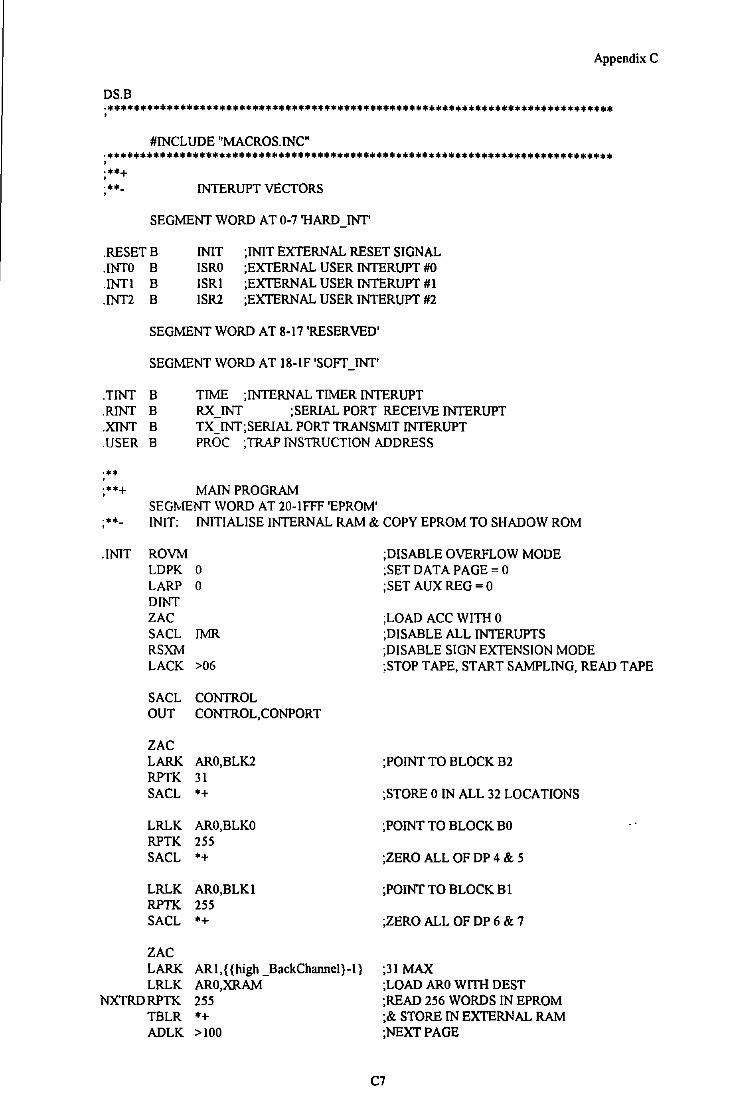
Appendix C

DS.B •••••••••••••••••••••••••••••••••••••••••••••••••••••••••••••••••••••••••••••• •

#INCLUDE "MACROS.INC" •••••••••••••••••••••••••••••••••••••••••••••••••••••••••••••••••••••••••••••• . ;**+ ..... . INTERUPT VECTORS

SEGMENT WORD AT 0-7 'HARD_INT'

.RESETS

.INTO 8

.INTI 8

.INT2 8

INIT ;INJT EXTERNAL RESET SIGNAL ISRO ;EXTERNAL USER INTERUPT #0 !SRI ;EXTERNAL USER INTERUPT #1 ISR2 ;EXTERNAL USER INTERUPT #2

SEGMENT WORD AT 8-17 'RESERVED'

SEGMENT WORD AT 18-IF 'SOFT_INT'

.TINT 8

.RINT 8

.XINT 8

.USER 8

TIME ;INTERNAL TIMER INTERUPT RX_INT ;SERIAL PORT RECEIVE INTERUPT TX_INT;SERIAL PORT TRANSI\1IT INTERUPT PROC ;TRAP INSTRUCTION ADDRESS

... . ;••+ MAIN PROGRAM

SEGl'vrENT WORD AT 20-IFFF 'EPROM' ;**- !NIT: INITIALISE INTERNAL RAM & COPY EPROM TO SHADOW ROM

.!NIT ROVM LDPK 0 LARP 0 DINT ZAC SACL lMR RSXM LACK >06

SACL CONTROL OUT CONTROL,CONPORT

ZAC LARK ARO,BLK2 RPTK 31 SACL •+

LRLK ARO,BLKO RPTK 255 SACL •+

LRLK ARO,BLKl RPTK 255 SACL *+

ZAC LARK ARl,{ {high _BackChannel}-1} LRLK ARO,XRAM

NXTRD RPTK 255 TBLR •+ ADLK >100

;DISABLE OVERFLOW MODE ;SET DATA PAGE= 0 ;SET AUX REG = 0

;LOAD ACC WITH 0 ;DISABLE ALL INTERUPTS ;DISABLE SIGN EXTENSION MODE ;STOP TAPE, START SAMPLING, READ TAPE

;POINT TO BLOCK 82

;STORE 0 IN ALL 32 LOCATIONS

;POINT TO BLOCK 80

;ZERO ALL OF DP 4 & 5

;POINT TO BLOCK 8 l

;ZERO ALL OF DP 6 & 7

;31 MAX ;LOAD ARO WITH DEST ;READ 256 WORDS IN EPROM ;& STORE IN EXTERNAL RAM ;NEXT PAGE

C7

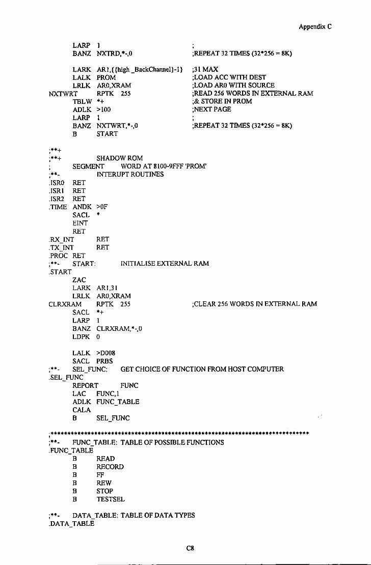
LARP BANZ NXTRD, •-,0

LARK ARI,{{high_BackChannel}-1} LALK PROM LRLK ARO,XRAM

;REPEAT 32 TIMES (32*256 = 8K)

;31 MAX ;LOAD ACC WITH DEST ;LOAD ARO WITH SOURCE

Appendix C

NXTWRT RPTK 255 TBLW *+

;READ 256 WORDS IN EXTERNAL RAM ;& STORE IN PROM

ADLK >LOO ;NEXT PAGE LARP I BANZ NXTWRT, *-,0 ;REPEAT 32 TIMES (32*256 = 8K) B START

·••+ . ·••+ . SHADOW ROM

SEGMENT WORD AT 8100-9FFF 'PROM'

···-. RET RET RET

INTERUPT ROUTINES . ISRO .!SRI .ISR2 .TIME ANDK >OF

SACL * ElNT RET

.RX lNT

.TX INT

.PROC RET

RET RET

;**- START: INITIALISE EXTERNAL RAM .START

ZAC LARK LRLK

CLRXRAM

ARI,3 I ARO,XRAM RPTK 255

SACL *+ LARP BANZ LDPK

CLRXRAM, *-,0 0

LALK >0008 SACL PRBS

;CLEAR 256 WORDS IN EXTERNAL RAM

;**- SEL_FUNC: GET CHOICE OF FUNCTION FROM HOST COMPUTER .SEL_FUNC

REPORT FUNC LAC FUNC,I ADLK FUNC TABLE CALA B SEL FUNC

•••••••••••••••••••••••••••••••••••••••••••••••••••••••••••••••••••••••••••••• ' ;**- FUNC_TABLE: TABLE OF POSSIBLE FUNCTIONS .FUNC_TABLE

B READ B RECORD B FF B REW B STOP B TESTSEL

;**- DATA_TABLE: TABLE OF DATA TYPES .DATA_TABLE

CS

DATA_O DATA I DATA_2 DATA_3 B

B WRT_PRBS B WRT_SAW B WRT_SQR

WRT_SEQ

;**- CODE_ TABLE: TABLE OF CODING ALGORITHMS .CODE_ TABLE CODE_O B CODE_! B CODE_2 B CODE_3 B CODE_4 B CODE_5 B CODE_6 B

;**- TEST_TABLE:

MANWRT MILLWRT MIL2WRT ISSWRT WRT3PM CRAWRT NRZIMAN

TABLE OF TEST ROUTINES .TEST _TABLE

B B B B

ECHO TSTBCHGET TSTBCHSND TSTXRAM

AppendixC

·***************************************************************************** ' ;**+ READ: .READ CALL NXTREAD

READ DATA ON TAPE AND SEND IT TO THE PC

LRLK LARP

MORE LRLK LARK CALL

NXTCHLAC SACL BANZ LARP BANZ

PLAY LRLK ARO,XRAM AR7,2047 I ARI,ADCI AR2,3 SAMPLE *+,0,0 *+,0,2 NXTCH,*-,1 7 MORE,*-,1

LRLK ARO)CRAM LRLK AR7,8191 LARP 0

OUTNXT LARK AR4,7 LAC *+,0,4

FUDGEROR SACL TEMP LAC DATA ROL SACL DATA LAC TEMP BANZ FUDGE,*­LARP 7 WRPORT DATA BANZ OUTNXT, *-,0 B NXTREAD

.SAMPLE LACK AND SACL OUT

>OF CONTROL CONTROL CONTROL,CONPORT

;play tape

;sample and convert all channels ;load ace with adc data ;store in xram ;repeat for all 4 channels

;repeat until xram full

;(2048*4)-1

;fix adc data bus inversion

;send data to PC ;repeat untill all data has been sent

;RESET 4 MSB'S

;sample data on all channels

C9

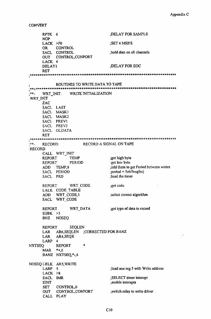
CONVERT

RPTK 6 NOP LACK >FO OR CONTROL SACL CONTROL OUT CONTROL,CONPORT LACK 4 DELAY! RET

Appendix C

;DELAY FOR SAMPLE

;SET4 MSB'S

;hold data on all channels

;DELAY FOR EOC

·***************************************************************************** . ROUTINES TO WRITE DATA TO TAPE

·**+************************************************************************** . ;*"'- WRT_INIT: WRITE INITIALIZATION .WRT_INIT

ZAC SACL LAST SACL MASK! SACL MASK2 SACL PREVI SACL PREV2 SACL OLDATA RET

·***************************************************************************** . ;**- RECORD: RECORD A SIGNAL ON TAPE .RECORD

CALL WRT_INIT REPORT TEMP REPORT PERIOD ADD TEMP,S SACL PERIOD SACL PRD

REPORT \VRT CODE LALK CODE TABLE ADD WRT_CODE,l SACL WRT_CODE

REPORT \VRT DATA SUBK >3 BNZ NOSEQ

REPORT SEQLEN

;get high byte :get low b~1e ;add them to get Period between writes ;period = 5e6/freq(hz) ;load the timer

;get code

;select correct algorithm

;get type of data to record

LAR AR6,SEQLEN ;CORRECTED FOR BANZ LAR AR4,SEQX LARP 4

NXTSEQ REPORT * MAR *+,6 BANZ NXTSEQ,*-,4

NOSEQLRLK LARP LACK SACL EINT SET OUT CALL

AR5,WRITE 5 >S lMR

CONTROL,O CONTROL,CONPORT PLAY

;load aux reg 5 with Write address

;SELECT timer interupt ;enable interupts

;switch relay to write driver

CIO

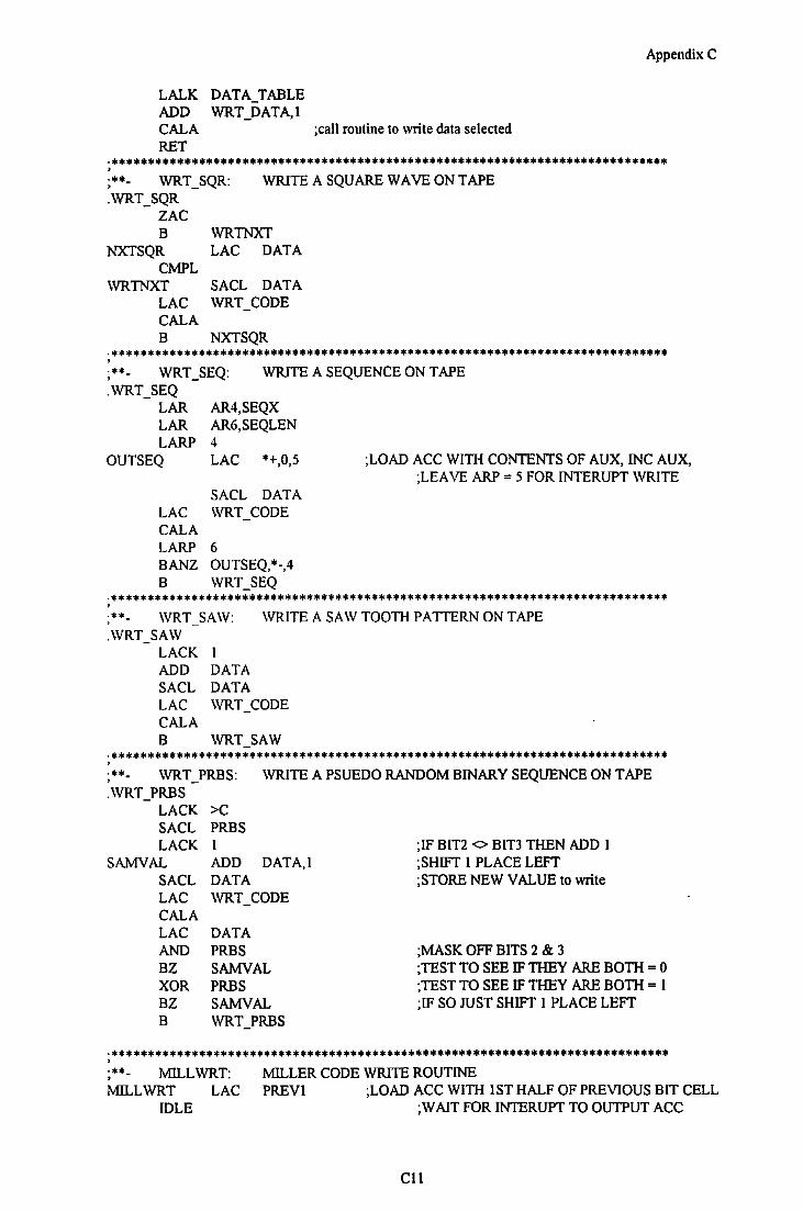
LALK ADD CALA RET

DATA TABLE WRT_DATA,l

AppendixC

;call routine to write data selected

•••••••••••••••••••••••••••••••••••••••••••••••••••••••••••••••••••••••••••••• ' ;**- WRT_SQR: WRITE A SQUARE WAVE ON TAPE .WRT_SQR

ZAC B

NXTSQR CMPL

WRTNXT LAC DATA

WRTNXT SACL DATA LAC WRT_CODE CALA B NXTSQR

•••••••••••••••••••••••••••••••••••••••••••••••••••••••••••••••••••••••••••••• ' ;**- WRT_SEQ: WRITE A SEQUENCE ON TAPE .\VRT_SEQ

LAR LAR LARP

OUTSEQ

LAC CALA LARP 8ANZ 8

AR4,SEQX AR6,SEQLEN 4 LAC *+,0,5

SACL DATA \VRT CODE

6 OUTSEQ,*-,4 WRT_SEQ

;LOAD ACC WITH CONTENTS OF AUX, INC AUX, ;LEAVE ARP = 5 FOR INTERUPT WRITE

•••••••••••••••••••••••••••••••••••••••••••••••••••••••••••••••••••••••••••••• , ·** \VRT SAW: \VRITE A SA \V TOOTH PATTERN ON TAPE .WRT_SAW

LACK ADD SACL LAC CALA 8

I DATA DATA \VRT_CODE

\VRT_SAW •••••••••••••••••••••••••••••••••••••••••••••••••••••••••••••••••••••••••••••• , ;**- WRT_PRBS: WRITE A PSUEDO RANDOM BINARY SEQUENCE ON TAPE .\VRT PRBS

LACK >C SACL PRBS LACK I

SAMVAL ADD DATA,! SACL DATA LAC \VRT CODE CALA LAC AND 8Z XOR 8Z 8

DATA PRBS SAMVAL PRBS SAMVAL \VRT_PRBS

;IF BIT2 <> BIT3 THEN ADD I ;SHIFT I PLACE LEFT ;STORE NEW VALUE to write

;MASK OFF BITS 2 & 3 ;TEST TO SEE IF THEY ARE BOTH = 0 ;TEST TO SEE IF THEY ARE BOTH = I ;IF SO ruST SHIFT I PLACE LEFT

•••••••••••••••••••••••••••••••••••••••••••••••••••••••••••••••••••••••••••••• , ;**- MILL\VRT: MILLER CODE WRITE ROUTINE MILLWRT LAC PREVl ;LOAD ACC WITH 1ST HALF OF PREVIOUS BIT CELL

IDLE ;WAIT FOR INTERUPT TO OUTPUT ACC

Cll

LAC IDLE LAC CMPL SACL LAC SACL CMPL AND XOR SACL XOR SACL RET

Appendix C

PREV2 ;LOAD ACC WITH 2ND HALF OF PREVIOS BIT CELL

OLD ATA

TEMP DATA OLD ATA

TEMP PREV2 PREVI DATA PREV2

;WAIT FOR INTERUPT TO OUPUT ACC

;GET COMPLEMENT OF PREVIOUS DATA

;UPDATAOLDATA WITH CURRENT DATA ;GET COMPLEMENT OF CURRENT DATA

;AND WITH COMPLEMENT OF PREVIOUS DATA ;XOR WITH 2ND HALF OF PREVIOUS BIT CELL ;STORE THE 1ST HALF OF CURRENT BIT CELL ;XORCURRENTDATA ;STORE THE 2ND HALF OF CURRENT BIT CELL

·***************************************************************************** ' ;**- MIL2WRT: MILLER SQUARED WRITE ALGORITHM MIL2WRT LAC

IDLE PREVI ;LOAD V AL WITH 1ST HALF OF PREVIOUS BIT CELL

;WAIT FOR INTERUPT TO OUTPUT ACC

CELL

CL KIT LAC AND AND XOR SACL

IDLE LAC AND SACL LAC ClviPL SACL LAC SACL CMPL AND XOR SACL XOR XOR SACL

RET

OLDATA DATA MASK I PREV2 PREV2

OLD ATA DATA MASK I OLDATA

TEMP DATA OLD ATA

TEMP PREV2 PREVI DATA MASK I PREV2

;GET TRACKS WITH CONSEQUTIVE 'l's ;ISSOLATE TRACKS WITH EVEN NUMBER OF ONES

;XOR WITH 2ND HALF OF PREVIOS BIT

;WAIT FOR INTERUPT TO OUPUT ACC

;UPDATEMASK1

;GET COMPLEMENT OF PREVIOUS DATA

;GET COMPLEMENT OF CURRENT DATA ;AND WITH COMPLEMENT OF PREVIOUS DATA ;XOR WITH 2ND HALF OF PREVIOUS BIT CELL ;STORE THE 1ST HALF OF CURRENT BIT CELL

;XOR CURRENT OAT A

·***************************************************************************** ' ;**- MANWRT: WRITE DATA ON TAPE IN MANCHESTER CODE .MANWRT LAC DATA

CMPL IDLE ; WAIT FOR INTERUPT TO OUTPUT V AL LAC DATA IDLE ;WAIT FOR INTERUPT TO OUTPUT V AL RET

•••••••••••••••••••••••••••••••••••••••••••••••••••••••••••••••••••••••••••••• ' ;**- NRZIMAN: .NRZIMAN

LAC DATA CMPL XOR OLDATA SACL OLDATA IDLE LAC DATA

Cl2

XOR SACL IDLE RET

OLD ATA OLD ATA

Appendix C

·***************************************************************************** ' ;*"'- ISSWRT: WRITE DATA ON TAPE IN !SS 2/3 RATE CODE .ISSWRT

ISS_PT2

LAC SACL OR SACL LALK SACL RET

CMPL AND NRZI IDLE

LAC CMPL AND AND SACL LAC AND OR AND NRZI IDLE

LAC CMPL AND CMPL SACL LAC CMPL AND AND NRZI IDLE

LAC SACL LAC SACL LAC SACL LALK SACL RET

DATA OLD ATA PREV2 MASK I ISS_PT2 WRT_CODE

LAC PREVI

MASK2

MASK I

PREY! DATA TEMP PREY! PREY2 TEMP MASK2

MASK!

DATA

TEMP PREV2

TEMP MASK2

MASK! MASK2 OLDATA PREVI DATA PREV2 ISSWRT WRT_CODE

;TEST FOR ZEROS IN BITS 2&3

;***************************************************************************** ;**- 3PMWRT: WRITE DATA ON TAPE IN 3PM CODE .WRT3PM

LAC DATA SACL PREVI LALK PM PT2

ClJ

Appendix C

SACL WRT_CODE RET

.PM_PT2 LAC DATA SACL PREV2 LALK PM_OUT SACL WRT_CODE RET

.PM_OUT LALK WRT3PM SACL WRT_CODE LAC PREV2 OR DATA AND PREVI AND OLDATA SACL MASK!

LAC OLDATA XOR MASK! NRZI

P5 OUT IDLE

LAC MASK! NRZI

P6 OUT IDLE

PI CALC LAC PREV2 OR DATA AND PREVI XOR MASK! NRZI

PI OUT IDLE

P2_CALC LAC PREVI CMPL AND PREV2 NRZI

P2 OUT IDLE

P3_CALC LAC PREV2 OR DATA CMPL AND PREVI NRZI

P3_0UT IDLE

P4 CALC LAC PREVI XOR PREV2 CMPL AND DATA NRZI

P4 OUT IDLE

P5_CALC LAC DATA OR PREVI OR PREV2 CMPL SACL TEMP LAC PREVI XOR DATA

Cl4

Appendix C

AND PREV2 OR TEMP SACL OLDATA

RET

·***************************************************************************** ' ;**- CRAWRT: WRITEDATAONTAPEINCRACODE WRT _AC MACRO CYCLES

LOCALACWRT LARK AR7,CYCLES

ACWRT LACK >F NRZI IDLE LARP 7 BANZ ACWRT,*-,5 I\1END

.CRAWRT LAC DATA SACL PREVI LALK CRA_PT2 SACL WRT_CODE RET

.CRA_PT2 LAC DATA SACL PREV2 LALK CRA_OUT SACL WRT_CODE RET

CRA_OUT WRT_AC 5

LAC PREVI CMPL SACL TEMP AND PREV2 SACL MASK!

LAC PREV2 CMPL AND TEMP SACL MASK2

LAC DATA CMPL SACL OLDATA AND TEMP SACL TEMP LAC PREV2 CMPL AND PREY! OR TEMP SACL TEMP LAC LAST AND MASK! XOR TEMP LARK AR7,15

WRTBISACL LAST IDLE

;temp= not prevl

;mask! =not prevl and prev2

;mask2 =not prevl and not prev2

;oldata = not data

;temp =not prev I and not data

;temp= (not prev2 and prevl) or (not prevl and not data)

;mask of last data bits to change

Cl5

XOR LARP BANZ

MASK! 7 WRTBI,*-,5

WRT_AC 5

LARK LAC AND XOR

WRTB2SACL IDLE XOR LARP BANZ

AR7,15 LAST MASK2 OLD ATA LAST

MASK2 7 WRTB2,*-,5

WRT_AC 5

LALK CRAWRT SACL WRT CODE RET

Appendix C

·***************************************************************************** '

CONTROLS FOR THE TAPE DECK ·***************************************************************************** ' ;**- REW: .REW CALL

RESET SET OUT CALL RET

REWIND TAPE STOP CONTROL,2 CONTROL,! CONTROL,CONPORT SOLDLY

;DISABLE FAST FORWARD SOLENOID

;DELAY WHILE SOLENOIDS ENGAGE

·***************************************************************************** '

FF: FAST FORWARD TAPE . **-' .FF CALL STOP

SET CONTROL,2 RESET CONTROL, l OUT CONTROL,CONPORT CALL SOLDLY RET

;DISABLE REWIND SOLENOID ;ENABLE FAST FORWRD SOLENOID

;DELAY WHILE SOLENOIDS ENGAGE

·+++++++++++++++++++++++++++++++++++++++++++++++++++++++++++++++++++++++++++++ ' ;**- STOP: .STOP SET

SET OUT CALL RET

STOPS THE TAPE CONTROL,2 CONTROL,! CONTROL,CONPORT SOLDLY

;DISABLE REWIND SOLENOID ;DISABLE FAST FORWARD SOLENOID

·***************************************************************************** ' ;**- PLAY: PLAY THE TAPE .PLAY RESET CONTROL,2

RESET CONTROL, l OUT CONTROL,CONPORT CALL SOLDLY RET

;ENSBLE REWIND SOLENOID ;ENABLE FAST FORWARD SOLENOID

;DELAY WHILST SOLENOIDS ENGAGE

·***************************************************************************** ' ;**- SOLDLY: SOLENOID DELAY .SOLDLY LALK >1000,3 ;LOAD ACC WITH >40000 (262144)

DELAY! ;Ius DELAY LOOP REPEATS UNTIL ACC = 0 RET

·***************************************************************************** '

Cl6

Appendix C

... _ MO NIT: MONITOR HALL EFFECT TRANSISTOR TO SEE WHEN TAPE . ENDS ;NOTE HALL EFFECT TRANSISTOR MUST BE CONNECTED TO BIT I 1 OFT APE READ liP PORT

.MONITLRLK LARK LRLK LARP

BLKD REPMON

XOR ANDK BNZ BANZ LARP BANZ

MONEND RET

ARl,>FFFF AR0,2 AR7,ADC1 7

ADCl,TEMP LAC TEMP *,1 >0800 ;MASK OFF BIT 11 MONIT; REPMON,*-,7 0 REPMON,*-,7 CALL STOP

;LOAD ARl WITH LONG DELAY ;LOAD ARO WITH SHORT DELAY

;READ FROM ANY ADC

;STOP THE TAPE

·**+************************************************************************** . TEST ROUTINES

·***************************************************************************** ' ;**- TESTSEL: SELECT TEST ROUTINE .TESTSEL

REPORT FUNC LAC FUNC,I ADLK TEST_ TABLE CALA RET

·***************************************************************************** , ·••- ECHO: ECHO'S INPUT FROM PC .ECHO LARK AR0,255

LARP 0 ECHO I REPORT TEMP

WRPORT TEMP BANZ ECHOI,*­RET

•••••••••••••••••••••••••••••••••••••••••••••••••••••••••••••••••••••••••••••• . ;**- TSTOP: TEST OUTPUT TO PC- SEND 0, 1,2 ... FF . .TSTOP LARK AR5,DATA

LARP 5 ZAC

CNTOUT SACL • WRPORT • ADDK I B CNTOUT RET

•••••••••••••••••••••••••••••••••••••••••••••••••••••••••••••••••••••••••••••• . ;••- TSTSTRB: PULSE STROBE LINE .TSTSTRB

SXF RXF B TSTSTRB

•••••••••••••••••••••••••••••••••••••••••••••••••••••••••••••••••••••••••••••• . ..•. . TSTIME: TEST INTERNAL TIMER

Cl7

.TSTIME LACK SACL LACK SACL

REPTIM B

LDPK 0 >10 PRD 8 IMR IDLE REPTIM

AppendixC

;ENABLE TIMER INTERUPT ONLY

•••••••••••••••••••••••••••••••••••••••••••••••••••••••••••••••••••••••••••••• , ;**- TSTCNTL: PULSE CONTROL LINES .TSTCNL LARP 5

LARK ARS,CONTROL REPTST LACK >FF

SACL * OUT *,CONPORT ZAC SACL * OUT *,CONPORT B REPTST RET

•••••••••••••••••••••••••••••••••••••••••••••••••••••••••••••••••••••••••••••• , ·**- TSTADC: . TST ADC LRLK

TEST ADC SELECT LINES AR7,ADCI

LARP 7 RPTK J LAC *+ B TSTADC

•••••••••••••••••••••••••••••••••••••••••••••••••••••••••••••••••••••••••••••• ~··- TSTXRAM: .TSTXRAM

LRLK ARO,XRAM LRLK ARI,8191 LARP 0

NXTADDR LALK >AAAA SACL • SUB * BNZ XRAMERR LALK >5555 SACL • SUB • BNZ XRAMERR MAR *+,1 BANZ NXTADDR:-,o ZAC

XRAMERR SACL DATA WRPORT DATA RET

•••••••••••••••••••••••••••••••••••••••••••••••••••••••••••••••••••••••••••••• , ;**- TSTROM: .TSTROM LARK ARI,J l

LALK PROM LRLK ARO,XRAM LARP 0

NXTBLK RPTK 255 TBLR *+ LARP BANZ NXTBLK, *-,0

LDPK LRLK

NXTBYTE

0 ARO,XRAM LAC *+

Cl8

1RPTK. 7 ROR SAC_~_ DATA WRJ!ORT .DA;r:A: RPTK 7 ~R.oL SAC~ DATA WRP0RT DA;r:A B NXFBYTE

'. * ..... * ••• * *. * ... * ·-·~·-......... _._ ••••••.• -· .••• •:·~·-.:• ··~ •• -._._. ·-· .. -._. ·····:•-·-· ........ -·-· * ·~· '4<+:• •• ·-•• ; ,,

~END

Cl9.

Appendix C

.ST ADDR DS.B THIS FILE CONTAINS SOME COMMONLY USED MACROS

' ·***************************************************************************** ' ·••- INC: INCREMENT ROUTINE: INCREMENT "PTR" AND TEST ITS WITHIN LIMITS ' ;PTR = PTR +I ;IF PTR > END THEN PTR = START

INC MACRO PTR,ST ART,END LOCAL INCEND

LAC ADDK SACL SBLK BLEZ LALK SACL

INCEND

PTR I PTR END INCEND START PTR MEND

•••••••••••••••••••••••••••••••••••••••••••••••••••••••••••••••••••••••••••••• ' ;**- DEC: DECREMENT ROUTINE: DCCREMENT "PTR" AND TEST ITS WITHIN LIM1TS

PTR=PTR-1 IF PTR <START THEN PTR =END

DEC MACRO PTR,START,END LOCAL DECEND LAC PTR SUBK I SACL PTR SBLK START BGEZ DECEND LALK END SACL PTR

DECEND MEND ·***************************************************************************** ; ••- SET: SET BIT ROUTINE SET MACRO LOC,BITPOS

LAC LOC ORK l,BITPOS SACL LOC MEND

•••••••••••••••••••••••••••••••••••••••••••••••••••••••••••••••••••••••••••••• ' ;**- RESET: RESET BIT ROUTINE RESET MACRO LOC,BITPOS

LAC LOC ORK l,BITPOS XORK I,BITPOS SACL LOC MEND

•••••••••••••••••••••••••••••••••••••••••••••••••••••••••••••••••••••••••••••• ' ;**- BIT: TEST BIT ROUTINE ;BIT MACRO BITPOS,MEM

LAC BIT,BITPOS AND MEM MEND

•••••••••••••••••••••••••••••••••••••••••••••••••••••••••••••••••••••••••••••• . ;**- SRL: SHIFT RIGHT LOGICAL SRL MACRO MEM,)CPLACES

LAC MEM, 16-XPLACES SACH MEM MEND

C20

Appendix C

•••••••••••••••••••••••••••••••••••••••••••••••••••••••••••••••••••••••••••••• • ;•*- SAVE: SAVE CURRENT PARAMETERS WITHOUT USING STACK

USES DATA PAGE 0

STORE MACRO SST STATUS SSTI STATUS I LDPK 0 SACL ACCL SACH ACCH MEND

;SAVE STATUS REG. STO ;SAVES STATUS REG. STI ;CHANGE TO DATA PAGE 0 ;SAVE ACCUMULATOR

•••••••••••••••••••••••••••••••••••••••••••••••••••••••••••••••••••••••••••••• . ;**- RESTORE: RESTORES SAVED PARAMETERS RESTORE MACRO

LDPK 0

ZALH ADDS LST LSTI MEND

ACCH ACCL STATUS STATUS!

;GOTO DATA PAGE I TO RESTORE PRE­;INTERUPT CONDmONS ;RESTORE ACCUMULATOR

;RESTORE STO ;RESTORE STI

•••••••••••••••••••••••••••••••••••••••••••••••••••••••••••••••••••••••••••••• ' ·**- DELAY!: IuS DELAY* ACC DELAY! MACRO

LOCAL DELJI DELJI SUBK I

RPTK 4 NOP BNZ DELJI MEND

; I uS DELAY LOOP UNTIL ACC = 0

•••••••••••••••••••••••••••••••••••••••••••••••••••••••••••••••••••••••••••••• ; **- TST APE: TEST TAPE IS MOVING TST APE MACRO DEST

LOCAL CHANGED,NOTEND,NOTST LAC BIT,4 AND CHANGE BNZ CHANGED

BANZ LAC SUB BGZ CALL LAC SACL B

CHANGED NO TEND NOTST MEND

NOTST MOVING ONE NOTEND STOP ONE,IO MOVING DEST

LAC · ONE,IO SACL MOVING

•••••••••••••••••••••••••••••••••••••••••••••••••••••••••••••••••••••••••••••• . ;**- SELFUNC: SELECT A GIVEN FUNCTION SELFUNC MACRO FNUM,MASK,ROUTINE

LOCAL NOTSEL LACK >FNUM SACL TEMP LACK >MASK AND FUNC SUB TEMP BNZ NOTSEL

C21

AppendixC

CALL ROUTINE NOTSEL I\IIEND •••••••••••••••••••••••••••••••••••••••••••••••••••••••••••••••••••••••••••••• ' ;u. NRZI: CONVERT ACC TO NRZI FORMAT NRZI MACRO

XOR LAST SACL LAST IVIEND

•••••••••••••••••••••••••••••••••••••••••••••••••••••••••••••••••••••••••••••• '

ROUTINES TO COMMUNICATE TO EXTERNAL DEVICES VIA PARALLEL PORT •••••••••••••••••••••••••••••••••••••••••••••••••••••••••••••••••••••••••••••• ' ···­'

REPORT: READ PARALLEL PORT

REPORT MACRO PDATA;READPARALLELPORT LOCAL STRBLO,STRBHI,STRBL02,STRBHI2 SXF ;SET BUSY

STRBLO BIOZ STRBLO ;WAIT FOR STROBE HIGH RXF ;NOT BUSY

STRBHI BIOZ STRBL02 ;WAIT FOR STROBE LOW B STRBHI

STRBL02 IN PDATA,PARPORT ;GET DATA FROM PARALLEL PORT SXF ;SET BUSY LINE LACK >FF AND PDATA ;ONLYSBITDATASOZEROOTHERBITS SACL PDATA

STRBHI2 BIOZ STRBHI2 ; \V AIT FOR STROBE TO GO HIGH I\IIEND

•••••••••••••••••••••••••••••••••••••••••••••••••••••••••••••••••••••••••••••• '

. ··-' WRPORT: WRITE TO PARALLEL PORT (HOST COMPUTER)

WRPORT MACRO PDAT A LOCAL BSYLO,BSYHI,NOTBSY SXF

NOTBSY BSYHI

;SET STROBE LINE HIGH BSYHI BIOZ

B NOTBSY

RXF OUT PDATA,PARPORT ;SEND DATA TO PARALLEL PORT

;SET STROBE LINE LOW BSYLO BIOZ BSYLO BUSY

SXF IVIEND

; WAIT FOR HOST TO GET DATA AND BECOI\IIE

;SET STROBE LINE HIGH

•••••••••••••••••••••••••••••••••••••••••••••••••••••••••••••••••••••••••••••• ' ·••-'

GETINP: GET INPUT FORM HOST COMPUTER

GETINP MACRO INPUT ;GET INPUT FROM PARALLEL PORT LOCAL STRBER,STRBHI,NXTRY,TSTFLG

SET CONTROL,13 SET CONTROL, 7 OUT CONTROL,LINES RESET FLAG,l

NXTRYBIT BZ IN LACK AND BZ

?,CONTROL STRBHI DATA,TAPE >80 DATA STRBER

;CONFIG PARALLEL PORT AS BUSY INPUT

;TEST STROBE LINE HIGH

C22

Appendix C

RESET CONTROL,7 OUT CONTROL,LINES ;SET BUSY LINE LOW

STRBHI IN DATA,TAPE LACK >80 ;WAIT FOR STRB TO GO LOW AND DATA BNZ STRBER IN INPUT,PARPORT ;GET DATA FROM PARALLEL PORT SET FLAG,l SET CONTROL, 7 ;SET BUSY LINE HIGH OUT CONTROL,LINES LACK >FF AND INPUT ;ONLY 8 BIT OAT A SO ZERO OTHER BITS

SACL INPUT

STRBER LAC DATA XOR OLDATA SACL CHANGE LAC DATA SACL OLDATA TSTAPE TSTFLG

TSTFLG BIT !,FLAG BZ NXTRY MEND

·***************************************************************************** ' ;**- OUTSIG: SEND AN OUTPUT SIGNAL OUTSIG MACRO

LAC ONE XOR CONTROL

SACL CONTROL OUT CONTROL,CONPORT MEND

·***************************************************************************** ' ·**- ERROR: ERROR MACRO

SEND AN ERROR MESSAGE TO HOST ERRNO

LACK >FF SACL TEMP \VRPORT LACK >00 SACL TEMP

TEMP

\VRPORT TEMP LACK ERRNO SACL TEMP WRPORT TEMP REPORT TEMP B START MEND

~··+··········································································

C23

A:p'pendixoD

Description of St_ate 'Fransiticm Matrix .and Finite $tate Transition

Dhtgrams for Run-: Length ~Limited iCod'es!

Dl

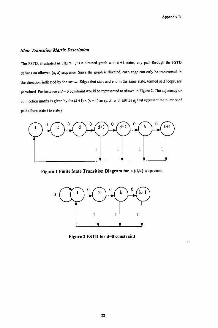
Appendix D

State Transition Matrix Description

The FSTD, illustrated in Figure I, is a directed graph with k +I states, any path through the FSTD

defines an allowed (d, k) sequence. Since the graph is directed, each edge can only be transversed in

the direction indicated by the arrow. Edges that start and end in the same state, termed self loops, are

permitted. For instance ad= 0 constraint would be represented as shown in Figure 2. The adjacency or

connection matrix is given by the (k +I) x (k + I) array, A, with entries aif that represent the number of

paths from state i to state j.

Figure l Finite State Transition Diagram for a (d,k) sequence

0

Figure 2 FSTD for d=O constraint

02

Appendix D

As an illustration, the following example displays the connection matrix for the (d, k) = (1,3)

constraints:

The n step state-transition matrix, A", has ij entries that give the number of distinct sequences from

state i to state j that are n bits long.

03

I

.. '

!'his rc.opy' of the ~thesis ihas beeri slipj:Hied. 1 .on .condition that anyone who consults it is

rUnclerstood to· recognise •that its :copyright Jests with ifs author and that .no :qUotatio11

from ,thdhesis and no irifonnation:derived.fr.om it may be· published withoul'the. auihors:

,prior;\vrittenrconsent

Copyright © 1994' by ~Paul James 1Davey

i