Municipal Solid Waste Management Problems: An Applied General Equilibrium Analysis

Welcome message from author
This document is posted to help you gain knowledge. Please leave a comment to let me know what you think about it! Share it to your friends and learn new things together.
Transcript

Municipal Solid Waste Management
Problems: An Applied General Equilibrium
Analysis

Promotor:
prof.dr. E.C. van Ierland, Hoogleraar Milieu-economie en Natuurlijke Hulpbronnen
Co-promotor:
dr. R.B. Dellink, Universitair Docent bij de leerstoelgroep Milieu-economie en
Natuurlijke Hulpbronnen
Samenstelling promotiecommissie:
prof.dr. G. Antonides (Wageningen Universiteit)
prof.dr.ir. W.J.M. Heijman (Wageningen Universiteit)
prof.dr. P. Rietveld (Vrije Universiteit Amsterdam)
prof.dr. T. Sterner (Göteborg University)

Heleen Bartelings
Municipal Solid Waste Management
Problems: An Applied General Equilibrium
Analysis
Proefschrift
ter verkrijging van de graad van doctor
op gezag van de rector magnificus
van Wageningen Universiteit,
Prof.dr.ir. L. Speelman,
in het openbaar te verdedigen
op maandag 1 december 2003
des namiddags te vier uur in de Aula

Bartelings, H.
Municipal solid waste management problems, an applied general equilibrium analysis
/H. Bartelings
PhD thesis Wageningen University (2003) - with summaries and conclusions in
English and Dutch
ISBN 90-5808-925-8

i
Abstract
Bartelings, H. (2003) Municipal solid waste management problems: an applied
general equilibrium analysis. PhD thesis, Wageningen University, the Netherlands.
243 pp.
Keywords: Environmental policy; General equilibrium modeling; Negishi format;
Waste management policies; Market distortions.
About 40% of the entire budget spent on environmental problems in the Netherlands
is reserved for the waste management problem. Regardless of the amount spent on
waste management, the quantity of municipal solid waste generated still increases. It
has up till now proven impossible to decouple generation of municipal solid waste
and income growth.
This thesis investigates the policy options that can be used to reduce generation of
municipal solid waste and looks specifically at the direct and indirect effects of
introducing unit-based pricing. Two types of unit-based pricing are distinguished: a
full unit-based pricing scheme, in which municipalities charge a variable price for
collection of both organic waste and rest waste, and a selective unit-based pricing
scheme, in which municipalities only charge a unit-based price for the collection of
rest waste. It presents a modeling framework to simulate the waste market in the
Netherlands. The model includes several municipalities as sources of waste, consumer
preferences, economies of scale, transport costs, and several kinds of emissions
caused by waste treatment. In this thesis specific focus was given to the possibility of
waste leakage, where consumers pollute the organic waste stream with rest waste.
The model was used in a stylized example with numerical data based on the
Netherlands in 2000. The results show that the selective unit-based pricing scheme is
the most effective policy tool to reduce generation of municipal solid waste. Due to
the effects of waste leakage, however, it is not advisable to introduce unit-based
pricing in every municipality. The results show that it is not cost effective to introduce
selective unit-based pricing for waste collection in larger municipalities. In these
municipalities the effects of waste leakage are too costly. The degree of pollution is so
high that part of the organic waste stream cannot be composted and will have to be
incinerated, thus greatly increasing the costs of treating organic waste. Only in small
municipalities with a relatively large number of environmentally concerned
consumers selective unit-based pricing can be introduced. Larger municipalities may
consider introducing full unit-based pricing. This policy tool, however, only
stimulates prevention and not recycling, thus the effects for reducing generation of
rest waste are limited.

ii

iii
Voorwoord
Op het schrijven van een proefschrift zijn tal van zinspreuken van toepassing. Spreuken zoals
‘Aken en Keulen zijn niet op een dag gebouwd’, ‘de laatste loodjes wegen het zwaarst’ en ‘de
aanhouder wint’, waren zeker van toepassing op mijn proefschrift. Toch vind ik de stelling
van Ronday nog het meest toepasselijk: ‘Promoveren is vaak een weg naar niets en het gaan
naar nergens totdat je het bereikt hebt’. Na vijf jaar heb ook ik mijn doel bereikt en ligt het
proefschrift hier in gebonden vorm. Hoewel de weg zeker niet zonder hobbels is geweest en ik
me af en toe wanhopig afvroeg of het ooit wel wat zou worden, kan ik toch met voldoening en
plezier terugkijken op de afgelopen jaren en kan ik me nu vol overgave op mijn nieuwe werk
bij APE storten. Natuurlijk zou het me niet gelukt zijn zonder de hulp van anderen, die ik dan
ook in dit voorwoord wil bedanken.
Ten eerste natuurlijk mijn promotor Ekko van Ierland en co-promotor Rob Dellink die altijd
klaar stonden om vragen te beantwoorden, stukken door te lezen en commentaar te leveren
(dat hoewel niet altijd gewaardeerd, wel de kwaliteit van mijn proefschrift sterk heeft
verbeterd). Ook de MUSSIM-groep wil ik bedanken voor de interessante vergaderingen en de
stimulerende vragen die mij dwongen op geheel andere wijze naar mijn onderzoek te kijken.
Bert Hamelers van de leerstoelgroep Milieutechnologie en Thijs Oorthuys en Arjen
Brinkmann van Grontmij ben ik erkentelijk voor de uitleg en talrijke aanbevelingen met
betrekking tot de niet-economische aspecten van afvalverwerking.
Een woord van dank gaat ook uit naar mijn oud-collega’s van de leerstoelgroep Milieu-
Economie en Natuurlijke Hulpbronnen voor de prettige werksfeer en de hulp op welke wijze
dan ook bij het voltooien van mijn proefschrift. Speciaal wil ik hier Rolf Groeneveld
bedanken die al die jaren mijn kamergenoot is geweest en met wie ik menig al dan niet werk
gerelateerde discussies heb gevoerd. Ook wil ik al mijn vrienden, met name Gea, Judith, en de
oud Bak-cie, die altijd voor de steun en ontspanning zorgden hierbij bedanken. Een speciaal
woord van dank tenslotte voor mijn moeder en vader voor al de ondersteuning die zij mij de
laatste jaren hebben gegeven.
Tot slot wil ik onder het mom van ‘niemand te vergeten’ mijn kat Poemba bedanken die mij
tijdens de laatste maanden van intensief schrijven de broodnodige ontspanning bezorgde door
frequent languit op het toetsenbord te gaan liggen.
Den Haag, oktober 2003

iv

v
Table of contents
Part I Concepts and background
1 General introduction 3
1.1 Definition and classification 3
1.2 The waste management problem 5
1.3 Waste generation, market distortions and incentives 7
1.4 Objectives of the study 10
1.5 Conceptual framework 14
1.6 Outline of the thesis 17
2 Economics of waste management: key problems 21
2.1 Introduction 21
2.2 Waste generation: the optimal policy mix 23
2.2.1 Waste generation and the pricing mechanism 24
2.2.2 Finding the optimal policy mix 25
2.2.3 Elasticities of the demand for waste disposal services
and consumer attitudes towards recycling 34
2.3 The optimal mix of waste management methods 37
2.3.1 Financial cost problem 39
2.3.2 Social cost problem 40
2.3.3 Estimating environmental costs 43
2.4 Location problem of waste handling facilities 44
2.4.1 The spatial waste management problem:
an optimization approach 46
2.4.2 The spatial waste management problem:
an general equilibrium approach 49
2.3 Conclusions 50
3 Waste flows and management in the Netherlands : data and policies 53
3.1 Introduction 53
3.2 A general overview of waste flows in the Netherlands 55

vi
3.2.1 The composition of the municipal solid waste stream 56
3.3 Waste management policies 58
3.3.1 Waste management policies throughout the years 58
3.3.2 European waste management law 59
3.3.3 Municipalities and waste collection 60
3.4 Waste treatment options 64
3.4.1 Composting 65
3.4.2 Incineration 68
3.4.3 Landfilling 73
3.5 Concluding remarks 77
Part II Modeling waste management problems
4 Modeling market distortions in an applied general equilibrium
framework: the case of flat fee pricing in the municipal solid
waste market 81
4.1 Introduction 81
4.2 Description of the model 82
4.2.1 Introduction 82
4.2.2 The subsidy-cum-tax scheme 83
4.2.3 Description of the model including a unit-based price
for waste collection 84
4.2.4 Description of the model including a flat fee
for waste collection 90
4.2.5 Description of model including an upstream tax
for waste collection 92
4.3 A numerical example 93
4.3.1 Parameter values used in numerical example 93
4.3.2 Policy scenarios 96
4.3.3 Results 97
4.3.4 Sensitivity analysis 102
4.4 Conclusions 106
Appendix 4-A Solving a Negishi format 108
Appendix 4-B Definition of model indices, parameters and variables 109
vii
5 Economic incentives and the quality of municipal solid waste:
counterproductive effects through ‘waste leakage’ 111
5.1 Introduction 111
5.2 Modeling different waste qualities 113
5.2.1 General introduction to the model structure 113
5.2.2 The model represented in equations 115
5.3 A numerical example 118
5.3.1 Benchmark data 118
5.3.2 Results 122
5.3.3 Sensitivity analysis 124
5.4 Discussion and conclusions 129
Appendix 5-A Specification of relevant equations 131
Appendix 5-B Definition of indices, parameters, and variables 134
6 Modeling economies of scale, transport costs and the location
of waste treatment units in a general equilibrium framework 137
6.1 Introduction 137
6.2 Modeling the spatial aspects of the municipal solid waste problem 139
6.2.1 General introduction to the model structure 139
6.2.2 The model represented in equations 142
6.3 Model application and numerical analysis 146
6.3.1 The benchmark case 146
6.3.2 Scenarios 152
6.3.3 Results 157
6.4 Discussion and conclusions 167
Appendix 6-A Results of scenarios 169
Appendix 6-B Definition of indices, parameters, and variables 172
Part III Conclusions and recommendations
7 Summary, conclusions and recommendations 177
7.1 Introduction 177
7.2 The economic and environmental topics concerning the
municipal solid waste management problem 178

viii
7.3 The problems concerning the flat fee for waste collection 181
7.4 The problems of waste leakage 183
7.5 Choice of the optimal location of waste treatment units 186
7.6 Policy recommendations 187
7.7 Modeling of the waste problem 190
7.8 General conclusions 192
7.9 Research recommendations 193
Samenvatting, conclusies en aanbevelingen 195
References 213
Appendix I: Specification of the model in GAMS 225
Curriculum Vitae 243

1
Part I
Concepts and background

2
3
“ Waste itself is a human concept; everything in nature is eventually used. If
human beings carry on in their present ways, they will one day be recycled
along with the dinosaurs.” (Peter Marshall)
1 General introduction
1.1 Definition and classification
The majority of human activities will inevitably result in the generation of waste due
to the imperfect utilization of energy and resources. There are numerous definitions of
what exactly constitutes waste, and many classifications, which attempt to categorize
waste flows. According to the European Environmental Protection Act (1990), “waste
is any substance, which constitutes scrap material or any effluent or other unwanted
surplus substance arising from the application of a process, or any substance or
article, which requires to be disposed of as being broken, worn out, contaminated or
otherwise spoiled.”
Waste poses a highly complex and heterogeneous environmental problem. The
characteristics of waste are highly dependent on the materials of which it consists. For
example, the characteristics of nuclear waste and organic waste are very different,
both with respect to their natural absorption capacity and impact on human health. Yet
they have one thing in common: both waste types are by-products of human activity
and although they physically contain the same materials as found in useful products,
they differ from useful products due to their lack of value (White et al., 1997).
The existence, and more specifically, the treatment of waste can cause environmental
damage as well as health risks. Different categories of waste cause different problems.
For example, the health risks associated with toxic waste are much greater than those
relating to municipal solid waste. Depending on the type of waste that must be
handled, different legal regulations may be necessary to control the environmental and
economic effects of waste treatment.
Waste may be categorized with respect to the source that generated it (WMC, 2003d).
Waste types distinguished according to this classification are: (1) municipal solid
waste, which is generated by households and contains the so-called ‘rest waste’, as
well as organic waste, glass, paper and other recyclable materials (2) residual waste
that is generated by waste treatment facilities like composting units and incineration
plants, (3) industrial waste, which is generated by industrial sectors (4) construction

Chapter 1
4
waste, which is generated by the construction and demolition sectors, (5)
contaminated soil and (6) other waste, which is a diverse set of smaller types of waste
categories including, for example, waste originating from hospitals and non-
contaminated soil.
Other classifications, for example, based on composition of waste rather than its
origin, also exist. Such classifications regard toxic waste and organic waste as
separate categories. However, according to the above classification, toxic waste may
be included in every category: from municipal solid waste to other waste; organic
waste is part of both the category municipal solid waste and industrial waste.
In general, one can argue that there are five main categories of socially acceptable
waste handling options available, namely (1) prevention, (2) re-use and recycling, (3)
composting, (4) incineration and (5) landfilling. Naturally not every waste handling
option is suitable for every category of waste. Each waste handling option has its own
economic and environmental characteristics.
Waste prevention or minimization is usually the most favored waste handling option,
but may be difficult to achieve in our consumer society. Re-use and recycling of waste
have clear environmental advantages. By re-using and recycling materials, less virgin
materials need to be used, ultimately resulting in a closed production cycle in which
no or at least very few virgin materials are actually required. The economic costs of
re-use and recycling, however, are substantial, and there may be technical problems
preventing re-use and recycling on a large-scale. Moreover, it should be noted that
even recycling and re-use might cause environmental damage.
The first two categories are typical examples of ways of reducing waste flows. The
next three categories are examples of treating waste in order to get rid of it.
Composting organic waste is one of the most favored methods of waste treatment. By
transforming organic waste into compost, at least part of it can still be usefully
employed. In the Netherlands, the incineration of waste is the preferred way of
treating non-organic waste. Energy can be obtained through incinerating waste.
Incineration provides a major contribution to reaching the targets set by the European
government for the use of energy from renewable resources. Landfilling of waste,
which was predominant up until a decade ago, is the least preferred option for waste
treatment. Although it is relatively cheap, it also leads to relatively high
environmental risks due to emissions into the air and groundwater. In the Netherlands,
landfilling sites are legally required to provide permanent aftercare to reduce the
possibility of future spills.
The category hazardous waste deserves some special attention. According to the laws
of both the European Union and the United States, hazardous waste must be handled
more carefully than common municipal solid waste. Hazardous waste can either be a

General introduction
5
liquid, solid or sludge that is a by-product of a manufacturing process. It can also be
the result of commercial products, such as battery acid or industrial solvents, which
have been discarded. The treatment of this waste type can have serious environmental
effects. In the United States, hazardous waste may be landfilled but only in specially
designed and extra secure landfill sites. Since 2002, it is no longer possible to landfill
hazardous waste in the European Union; it must either be incinerated or treated in
another way. Following several scandals involving the dumping of hazardous waste in
developing countries, both the European Union and the United States have adopted
laws forbidding the export of hazardous waste.
1.2 The waste management problem
The increasing scale of economic activity, i.e. industrialization, urbanization, rising
standards of living and population growth, has led to a sharp increase in the quantity
of waste generated. The environment has a limited capacity for waste assimilation. If
too much waste enters the environment rather than being recycled or reused, the
assimilative capacity of the environment is put under too much stress to be able to
handle the total quantity of waste generated. This may result in pollution and resource
degradation and consequently economic damage (Turner, 1995).
According to the mass balance principle, which can be derived from the first law of
thermodynamics1, mass inputs must equal mass outputs for any process. This implies
that any virgin materials used in both the production and consumption process must
eventually be returned to the environment as higher entropy waste products or
pollutants (Ayres, 1989). It is not yet possible to achieve an one hundred percent
recycling rate. A society is, however, to some extent able to choose the quantity and
quality of waste it will generate.
Waste can be treated in several ways. It can be composted, incinerated, or landfilled.
Until a decade ago, landfilling of waste was very popular in the Netherlands.
Landfilling, however, is also the least environmentally friendly waste treatment
option. The government has, therefore, implemented several laws to render landfilling
less attractive. One of the most successful policy measures was the introduction of a
high landfilling tax. Due to this landfilling tax, landfilling became very expensive.
The price of landfilling combustible waste is actually higher than the cost of
incinerating it. This price incentive stimulated the industrial sectors to reduce waste
generation. Over the last 10 years, the overall recycling percentages in the industrial
1 The first law of thermodynamics, the law of conservation of mass/energy, states that physical
processes always require conservation of energy/mass. In other words, energy and matter cannot be
created or destroyed (Perman et al., 1996).

Chapter 1
6
sector increased from about 70% to almost 90%. Households recycle far less, only
about 40%. The government still faces a difficult task in trying to solve the municipal
solid waste problem.
The municipal solid waste flow accounts for about 40% of all waste that requires
treatment. This waste category presents perhaps the greatest waste management
problem in the Netherlands. By nature, municipal solid waste is one of the most
difficult sources of waste to manage due to its complex composition and diverse
sources of generation (Read, 1999). Since every household in the Netherlands
generates municipal solid waste, it is difficult to control this waste flow. To re-use,
recycle or compost waste, the government is dependent on the households. If a
household chooses to not recycle or separate waste, there is essentially nothing the
government can do, since it is far too expensive to check the quality and quantity of
waste recycled or composted in every household. Any attempt to reduce the municipal
solid waste flow by increasing the price of collection, usually results in some form of
illegal dumping. Consumers can, for example, dump waste in their neighbor’s bin,
take it to work with them, or dump it in a nearby field or forest. Households can also
illegally dispose of rest waste by dumping it in the organic or recyclable waste stream.
By polluting these waste streams they increase the costs of recycling and composting
significantly. The quantity of waste illegally disposed of differs a lot between
municipalities. Depending on the environmental preferences of the households, some
municipalities will have more significant problems with illegal disposal than others.
When designing an efficient waste management plan, it is important to consider the
interactions between the waste treatment sector, on the one hand, and the rest of the
economy on the other. Waste management policies aimed at reducing waste
generation at the production side ignore the behavior of the households such as the
choice of waste reduction and disposal decisions. The effects of the policy may
therefore be less beneficial than expected. Subsequently, policies designed to reduce
waste generation by private households can lead to households demanding products
with less waste content, thus influencing the producer decisions, but may also lead to
increased illegal disposal by private households.
Waste treatment costs are dependent on how and where the waste is treated. Due to
economies of scale, a smaller waste treatment unit is more expensive than a large one.
The quantity and quality of waste to be treated will have a significant impact on the
optimal location choice of waste treatment units. An efficient waste management plan
should take these spatial aspects into account. Each municipality should decide on the
basis of the quality and quantity of waste they collect, where and how to treat the
waste.
In short, a satisfactory analysis of municipal solid waste policies demands a
comprehensive framework in which production, consumption, disposal stages, and
General introduction
7
spatial aspects are included. In this thesis, such an analysis is presented. Using a
general equilibrium model of the waste market, I will demonstrate the effectiveness of
several waste management policies. My analysis will include the effects of consumer
preferences, recycling, prevention, economies of scale of waste treatment units,
transport costs and both quality and quantity of municipal solid waste.
1.3 Waste generation, market distortions and incentives
Following the Second World War, the generation of waste has increased rapidly in the
Netherlands. Since 1950, the quantity of waste generated has more than tripled, from
about 17 Mtonnes in 1950 to about 67 Mtonnes in 2000 (WMC, 2003e). During the
sixties and seventies in particular there was a sharp increase in national income, which
resulted in a substantial rise in waste generation. The European Environment Agency
(EAA, 2000) has demonstrated that waste generation in the European union is still
coupled with economic growth, making it impossible to pursue economic growth
without creating increasingly serious waste management problems. A particularly
close link exists between economic growth and the waste generated by the
construction industry, as well as between economic growth and municipal solid waste.
The generation of other types of waste, such as industrial and agricultural waste, is
still on the increase, but the quantity of these types of waste grows more slowly than
the annual rise in welfare due to successful implementation of waste management
policies (Dijkgraaf et al., 1999).
In the Netherlands, the government managed to decouple economic growth and the
generation of both industrial and construction waste. The generation of municipal
solid waste, however, is still clearly coupled with economic growth. The government
has failed to achieve its targets in this respect. This failure should be attributed
primarily to the presence of market distortions in the waste sector. Three important
factors have led to these market distortions, namely: (i) a flat fee-pricing system (ii)
virgin material biased regulations and (iii) the so-called ‘killer-contracts’.
The flat fee-pricing system generates the first market distortion. In a flat fee-pricing
scheme, the private households pay a fixed amount of money per year for the
collection of municipal solid waste. The total amount of the fee charged is not
dependent on the actual quantity of waste generated. Most municipalities choose this
kind of pricing system because it is quite expensive to keep track of the actual
quantity of waste generated per household. The most important problem created by
this pricing system is a missing link between waste generation and the price of
collection. Private households therefore have no price incentive to reduce the quantity
of waste they generate.

Chapter 1
8
Virgin material biased policies lead to the second market distortion. Virgin-material
biased policies inadvertently promote the use of virgin materials instead of recycled
materials. Miedema (1983) shows that because the price of waste collection and
disposal is not incorporated into the price of virgin materials, virgin materials are too
cheap in comparison to recycled materials. As long as the costs of waste disposal are
not internalized in the price of virgin materials, the demand for virgin materials will
be higher than socially optimal.
The third market distortion is one specific to the Netherlands. In the Netherlands, so-
called killer-contracts between municipalities and waste treatment facilities exist. The
killer-contracts between municipalities and incinerators have often been the focus of
discussion. However, to a lesser extent, killer-contracts also exist between
municipalities and composting units. These contracts specify the quantity of waste
that the municipality will deliver to the facility and the price they will pay for
disposing of it. These contracts provide the municipalities with an incentive to keep
the quantity of municipal solid waste generated by the private households constant so
that they can fulfill their contracts (see also De Jong and Wolsink, 1997).
Several studies have already analyzed the effects of market distortions in the
municipal solid waste market. An extensive overview of the current literature can be
found in Chapter 2. Most of these studies have concentrated on solving the problems
caused by the flat fee-pricing system. By replacing the flat fee-pricing system with a
unit-based pricing system, it is in theory possible to negate the market distortion. In a
unit-based pricing system, households pay a variable fee to the municipalities for the
collection of municipal solid waste; the fee charged will in some way depend on the
actual quantity of waste generated. Several differentiating pricing systems are
possible: for example a weight-based pricing system, which bases its price of
collection on the total weight of waste collected; a frequency-based pricing system,
which bases the price of collection on the frequency it is collected and a volume-
based pricing system, which bases its price on the volume of waste collected. In the
following paragraph, a brief overview is given of the most important articles in the
field of waste management and waste policies.
Wertz (1976) was the first to analyze the effects of a user charge on municipal solid
waste disposal. He found that there was a distinctive negative relation between the
price of municipal solid waste disposal and the actual quantity of municipal solid
waste generated.
Miedema (1983) analyzed the effects of other distorting characteristics of the
municipal solid waste market, such as virgin material-biased tax policies, virgin
material-biased policies, and indirect subsidization of virgin materials. He advocated
the introduction of virgin material taxes as a means of motivating efficient waste
disposal practice.
General introduction
9
Jenkins (1993) developed a model where households maximize utility, which
positively depends on the consumption of goods and negatively on the quantity of
recycling. A disposal charge for municipal solid waste collection is included in the
budget constraint. She found that the quantity of municipal solid waste generated is
sensitive to the price of municipal solid waste collection. In particular, she found that
the average price elasticity for municipal solid waste collection equaled –0.12.
Hong et al. (1993) derived a household recycling choice model and a demand
function for municipal solid waste disposal. They applied the model to a sample of
households from the Portland, Oregon metropolitan area and found a positive though
small relation between an increased price of waste collection and the quantity of
municipal solid waste generated.
Miranda et al. (1994) analyzed the effects of introducing a unit-based price on waste
disposal behavior. They collected data from 21 cities throughout the United States
over an 18-month period. They ascertained that introducing unit pricing and
recycling-programs could have a dramatic effect on the quantity of municipal solid
waste generated.
Sterner and Bartelings (1999) found that the introduction of an unit-based pricing
system for the collection of municipal solid waste combined with the launch of a
‘green’ shopping campaign and the introduction of recycling centers had a dramatic
effect on the quantity of municipal solid waste generated. This study focused on the
attitudinal variables that influenced the quantity of municipal solid waste generated by
households, and discovered that economic incentives, although important, are not the
only driving force behind the observed reduction of municipal waste. Given a proper
recycling structure, households are willing to invest more time in recycling and
composting than can be purely motivated by savings on their waste management bill.
Each of these empirical studies concludes that waste generation is sensitive to user
fees. The introduction of user fees can lead to a substantial reduction in municipal
solid waste generation, especially if they are combined with programs that increase
the public awareness about the municipal solid waste problem. The imprudent
construction of waste collection fees, however, might not have the desired effect and
can encourage illegal dumping, burning or other improper kinds of disposal (Fullerton
and Kinnaman, 1995).
Although most of these studies agree that a flat fee-pricing system is not optimal, they
differ on what the optimal policy to minimize cost of disposal should be. Studies like
Miedema (1983), Jenkins (1993), Strathman et al. (1995), and Linderhof et al. (2001)
propose the introduction of a ‘downstream’ tax, for example a unit-based pricing
system.

Chapter 1
10
Other studies, such as Fullerton and Kinnaman (1995,1996); Palmer and Walls
(1997); Fullerton and Wu (1998) and Choe and Fraser (1999), favor an ‘upstream’
tax, like a deposit refund system or an advanced disposal fee on price of the
consumption good, to internalize the waste treatment costs in the price of the product.
In a deposit-refund system, consumers pay an extra amount of money (the deposit) to
the seller. If the consumers return the remainder of the product to the seller, they will
get the deposit back. The recyclable waste that is thus collected is then sent to either a
re-use center or a recycling unit. They fear that a ‘downstream’ tax will be non-
optimal due to huge implementation and enforcement costs.
1.4 Objectives of the study
Recent literature, as described in Section 1.3, has provided some insights into the kind
of effects that market distortions can have on the municipal solid waste market. These
studies demonstrated how the introduction of a unit-based price, recycling subsidies
and taxes influenced both the quantity of municipal solid waste generated and the
total costs spent on waste treatment. These studies, however, have neglected several
important aspects of the waste management problem.
First of all, they have not fully considered the impact of the environmental
preferences of private households on the quantity and quality of waste they generate.
In this thesis, I will study how different types of consumers react to the introduction
of unit-based pricing for waste collection and how their preferences determine the
quality of waste they generate. Furthermore, I will show how these results may
influence the design of waste management plans.
Secondly, although some of these studies identified the illegal dumping of waste as a
household strategy for waste reduction, they did not consider an alternative method of
illegal disposal, namely the dumping of rest waste in the organic or recyclable waste
stream. This has important consequences for the treatment of organic and recyclable
waste, and in this thesis I will illustrate how this behavior can be included in the
analysis.
Thirdly, these studies did not cover the spatial aspects of the waste management
problem in the context of a general equilibrium analysis. Deciding where waste is to
be treated is an important aspect of the waste management problem and this decision
is influenced by both the quantity and the quality of waste that is generated. In this
thesis, a fixed set of waste management locations, several sizes of waste treatment
units, economies of scale, and transport costs are included in a general equilibrium
framework for the waste market.
In this thesis, I aim to contribute to the understanding of waste management in the
following ways:

General introduction
11
• By providing an analysis of how the incentive structure of the consumers,
emission restrictions, interrelations between the municipal solid waste sector and
the rest of the economy and the spatial aspects of the waste problem influence the
optimal municipal solid waste management plan.
• To assess whether a flat fee-pricing system, a unit-based pricing system for the
collection of rest waste, a unit-based pricing system for the collection of organic
and rest waste, or a recycling subsidy is the preferable policy option to minimize
the social costs of municipal solid waste treatment.
• To gain insight into how to develop a more efficient municipal solid waste
management plan, which solves inefficiencies caused by market distortions
present in the municipal solid waste market.
The objectives of this thesis lead to five key research questions:
1) What are the most important environmental and economic topics with regard
to the municipal solid waste management problem?
2) How does the market distortion caused by the flat fee-pricing system influence
municipal solid waste generation and how can these negative effects be
sufficiently reduced?
3) How great a problem is waste leakage and how is waste leakage influenced by
household attitudes?
4) How is the choice of the optimal location of waste treatment facilities
influenced by the quantity and quality of municipal solid waste generated by
consumers and, moreover, how will the spatial aspects of the municipal solid
waste management problem in turn influence the successfulness of introducing
unit-based pricing?
5) What kinds of policy changes can be recommended to minimize the total
social costs of municipal solid waste treatment for our society?
The first research question deals with the focus of the research project. On the basis
of a literature research, I will provide a detailed illustration of the municipal solid
waste management problem and outline the kind of environmental and economic
issues that are involved in it.
The second research question focuses specifically on one market distortion in the
municipal solid waste market, namely flat fee-pricing. As mentioned earlier, the flat
fee-pricing system can cause inefficiently high quantities of municipal solid waste to

Chapter 1
12
be generated. This thesis will pay special attention to the effects of the flat fee-pricing
system and policy alternatives.
The third research question deserves some introductory comments. The choice
between waste treatment options does not solely depend on the preferences of the
municipalities who collect municipal solid waste, but also on the kind of waste that is
generated. Not all waste is suitable for incineration or composting. For example,
municipal solid waste consists of several categories of waste, namely glass, paper,
hazardous waste, organic waste, and rest waste. The category rest waste is quite
diverse and consists of several different types of materials like plastics, aluminum, but
also glass, paper and organic waste. Glass and paper can be recycled, hazardous waste
must be incinerated or treated otherwise, and organic waste may be composted. Rest
waste will be incinerated. The recyclable and organic waste streams, however, should
not be polluted with rest waste. Dumping rest waste in the recyclable and organic
waste stream, which will subsequently be referred to as “waste leakage”, means that it
will be far more costly to treat this waste, for the rest waste has to be separated from
the other waste types.
The fourth research question concerns the interaction between the quality and
quantity of municipal solid waste and the choice of waste treatment units. To
minimize the cost of waste treatment, it is possible to concentrate only on minimizing
the quantity of municipal solid waste that is generated. In this case, the treatment of
waste is left out of the equation. Another method is to concentrate solely on how and
where municipal solid waste should be treated. Both of these methods, however, do
not consider the interactions between the quantity and the quality of waste generated
and the optimal waste treatment method. For example, a small quantity of organic
waste of a good quality could well be treated in a small composting unit. A large
quantity of waste of a lower quality may only be treatable in a larger composting unit.
As the quantity and quality of waste generated is not fixed, but may be influenced by
policies, it is important to take this interaction into account.
The choice for the optimal waste treatment location strongly depends on the
characteristics of the municipality concerned, the distance, the economies of scale,
and the environmental characteristics. Depending on both the quality and the quantity
of waste collected, municipalities may prefer either a smaller or a larger waste
treatment unit. Since municipalities are very diverse in size and nature, it is difficult to
design an optimal waste management plan that is suitable for every municipality. The
optimal municipal solid waste management plan must reflect the preferences of both
the municipalities and its inhabitants. Some municipalities may wish to charge
consumers for the quantity of waste they generate because of the ‘polluter pay
principle’, which says that every polluter should be charged for the environmental
costs they cause. Other municipalities may choose a flat fee due to the ‘equality
principle’, as poorer households will, in relative terms, pay more than more affluent
General introduction
13
households when a unit-based pricing system is implemented. It will, therefore, be
impossible to design an optimal national waste management plan without taking into
account the individual characteristics of the municipalities in question.
Finally the fifth research question concerns policy recommendations based on this
thesis. I will specifically illustrate the kind of situations in which it is advisable for a
municipality to introduce a unit-based pricing system for municipal solid waste
collection.
The focus of this thesis is to provide insight into the interrelations between the waste
sector, consumer behavior and the rest of the economy. The applied general
equilibrium technique will be used as a modeling technique. In particular, the Negishi
format is employed as the preferred modeling technique (see Section 1.5). To answer
the research questions, I will need to answer the following modeling questions:
a) How can interactions between the waste sector, government policies, and
the rest of the economy be modeled?
b) How can the flat fee-pricing system be introduced to a general equilibrium
setting?
c) How can spatial aspects of the waste management problem, such as a fixed
set of possible location of waste treatment units, economies of scale and
transport costs, be introduced to a general equilibrium framework?
This thesis is part of the research program Material Use and Spatial Scales in
Industrial Metabolism (MUSSIM), funded by The Netherlands Organization for
Scientific Research (NWO), which aims to develop an economic framework for
modeling the physical side of the economy in economic models. The research
program seeks to develop a framework and method of analysis that is based on
dynamic optimization and simulation. Furthermore, the program integrates economic
processes and decisions on the use of materials (environmental and resource
economics), physical flows and processes related to use of these materials (industrial
metabolism), and decisions on spatial allocation and transport affecting these
materials flows (regional and international economics).
The MUSSIM-research program is divided into three research projects. Each research
project examines a different aspect of material use in the economy. This thesis will
thus focus only on municipal solid waste streams in the Netherlands. I will, therefore,
disregard any possibilities of export of either waste or secondary materials. For
further information on the economic, environmental and social costs and benefits of
international trade in secondary materials at different spatial scales, see van Beukering
(2001). For more details on the relationship between material flows and economic and

Chapter 1
14
spatial structure of production in the Netherlands for selected materials and extensive
input-output models for the Dutch economy, see Hoekstra (2003).
1.5 Conceptual framework
The main modeling tool used in this thesis is the applied general equilibrium
modeling technique. I have chosen the general equilibrium setting because I would
like to analyze the main interactions between economic behavior, waste generation,
and resource use. The possibility of analyzing the interactions between several
markets at once is the strength of general equilibrium modeling. By choosing a
general equilibrium format it is possible to study the effects that a policy change
concerning municipal solid waste has on the waste treatment sector, the recycling
sector, the production sector and the virgin material sector.
Shoven and Whalley (1993) provide an excellent description of the main aspects of a
general equilibrium model:
“The term general equilibrium corresponds with the well-known Arrow-Debreu model (see
Arrow and Hahn, 1971). The number of consumers in the model is specified. Each consumer
has an initial endowment of N commodities and a set of preferences, resulting in demand
functions for each commodity. Market demands are the sum of each consumer’s demands.
Commodity market demands depend on all prices, and are continuous, nonnegative,
homogeneous of degree zero (i.e. no money illusion), and satisfy Walras’ law (i.e. that at any
set of prices, the total value of consumer expenditures equals consumer incomes). On the
production side, technology is described by either constant-returns-to scale activities or non-
increasing-returns-to-scale production functions. Producers maximize profits. The zero
homogeneity of demand functions and the linear homogeneity of the profits in prices (i.e.
doubling all prices doubles money profits) imply that only relative prices are of any
significance in such a model. The absolute price level has no impact on the equilibrium
solution Equilibrium in this model is characterized by a set of prices and levels of production
in each industry such that that the market demand equals supply for all commodities
(including disposals if any commodity is a free good). Since producers assumed to maximize
profits, this implies that in the constant-returns-to-scale case, no activity (or cost-minimizing
technique for production functions) does any better than break even at equilibrium prizes ”.
Shoven and Whalley (1993) p. 1-2
General equilibrium models are economy-wide models in the sense that they cover all
major economic transactions. The reason for modeling all relevant markets
simultaneously is the existence of complex interactions in an economy. Partial models
are based on the ceteris paribus conditions, i.e. the remainder of the economy is
assumed to be constant during policy simulations. As long as the ceteris paribus
condition holds, partial models are fine, and the complications and data-requirements
of general equilibrium models can be safely avoided. If, however, there are significant

General introduction
15
linkages between different markets, a partial analysis may lead to inaccurate and
perhaps biased results due to the existence of indirect effects2. In an extreme case, the
indirect effects, as captured by general equilibrium models, may outweigh the direct
effects, as captured by partial models. This can result in opposite policy
recommendation (Thissen, 1998).
General equilibrium models can be built in different formats, such as the Computable
General Equilibrium (CGE) format, the Negishi format, the full format, and the open
economy format. Each of these formats has its strengths and weaknesses, for more
information see Ginsburgh and Keyzer (1997). The models presented in this thesis are
all written in the Negishi format. I have chosen this format, as it is especially suitable
for the implementation of externalities, such as environmental pollution and waste
generation; and price rigidities, like a zero marginal price for waste collection. In
contrast to, for example, the CGE format, the Negishi format is able to calculate the
equilibrium solution in the case of price rigidities without requiring additional proof
that a general equilibrium solution has been found. Moreover, the Negishi format is
particularly suitable for incorporating multiple consumers given that it can maximize
several utility functions at the same time.
The Negishi format can, however, only be written in the primal form, which is a
weakness of this type of modeling. This means that in the model only production sets
exist. Prices are calculated exogenously from the model. In the primal format the
equilibrium solution if found by one or several mathematical programs using some
iterative procedure on parameters to find a fixed-point solution. In the dual form,
which for example is used in the computable general equilibrium format, net supply
and input demand are explicit functions of prices. The model is solved by a system of
nonlinear equations. The advantage of the dual form over the primal form lies in the
way in which the model is solved. As it is based on a system of nonlinear equations,
the computation and parameter estimation are normally far less difficult than the
computation in the primal form. Thus the dual form will find an equilibrium solution
much faster than the primal form. Nevertheless, I feel that this disadvantage does not
offset the strong points of the Negishi format.
In this thesis, the general equilibrium framework is used to analyze the interactions
between the waste treatment sector, the consumption sector, the production sector, the
recycling sector, and the extraction sector. The main elements of the conceptual
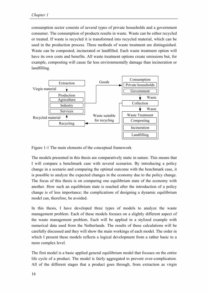
framework are shown in Figure 1-1. Several production sectors are distinguished.
Each of these production sectors uses virgin materials and recycled materials to
produce goods. These goods are consumed by the consumption sector. The
2 The indirect effects capture the interactions between different markets. Any change in one market can
result in a change within another, which in turn can again affect a change in the original market.
Chapter 1
16
consumption sector consists of several types of private households and a government
consumer. The consumption of products results in waste. Waste can be either recycled
or treated. If waste is recycled it is transformed into recycled material, which can be
used in the production process. Three methods of waste treatment are distinguished.
Waste can be composted, incinerated or landfilled. Each waste treatment option will
have its own costs and benefits. All waste treatment options create emissions but, for
example, composting will cause far less environmentally damage than incineration or
landfilling.
Extraction
Production
Services
Industry
Agriculture
Virgin material
Recycling
Consumption
Government
Private households
Collection
Waste Treatment
Composting
Incineration
Landfilling
Recycled material
Goods
Waste
Waste
Waste suitable
for recycling
Figure 1-1 The main elements of the conceptual framework
The models presented in this thesis are comparatively static in nature. This means that
I will compare a benchmark case with several scenarios. By introducing a policy
change in a scenario and comparing the optimal outcome with the benchmark case, it
is possible to analyze the expected changes in the economy due to the policy change.
The focus of this thesis is on comparing one equilibrium state of the economy with
another. How such an equilibrium state is reached after the introduction of a policy
change is of less importance; the complications of designing a dynamic equilibrium
model can, therefore, be avoided.
In this thesis, I have developed three types of models to analyze the waste
management problem. Each of these models focuses on a slightly different aspect of
the waste management problem. Each will be applied in a stylized example with
numerical data used from the Netherlands. The results of these calculations will be
carefully discussed and they will show the main workings of each model. The order in
which I present these models reflects a logical development from a rather basic to a
more complex level.
The first model is a basic applied general equilibrium model that focuses on the entire
life cycle of a product. The model is fairly aggregated to prevent over-complication.
All of the different stages that a product goes through, from extraction as virgin

General introduction
17
material, to production, consumption, recycling and final disposal by landfilling,
incineration or composting are included in the model. By including the entire lifecycle
of the product, it is possible to analyze how changes in generation of municipal solid
waste can affect the use of virgin and recycled materials, consumption patterns and
the choice of final waste disposal options.
The second model is more focused on the consumption sector and details of the waste
collection sector. Since the focus of the model is slightly less broad than the previous
model more detailed information about the different waste streams generated by
households and household preferences are included. In this model, the production
sectors are aggregated to one sector. Thus only one good is produced and consumed
in the model.
Finally, like the second model, the third model focuses on the consumption sector and
the waste treatment sector. In this model, detailed information about the spatial
aspects of the waste treatment problem, i.e. where waste is generated and where it
should be treated, are considered. Several municipalities and several locations of
waste treatment facilities will be included in the model. This model provides insight
into how changes in municipal solid waste generation influences the optimal location
of waste treatment units and thus the transport cost caused by transport of waste. The
analysis encompasses alternative settings for the locations of waste treatment units
given a set of locations and sizes of waste treatment units, economies of scale and
transport costs.
The models are all built in GAMS (General Algebraic Modeling System). This is an
optimization program, which is - among other things - quite suitable for building
complex general equilibrium models. The complete computer-code for each model is
shown in appendix I.
1.6 Outline of the thesis
To gain insight into how to develop the most efficient municipal solid waste
management plan, this thesis has been organized into seven chapters, starting with this
introduction (Chapter 1). This section describes the main contents of the subsequent
chapters in this thesis. Please note that the chapters have been written in such a way
that they can be read and published independently. Some explanations and footnotes
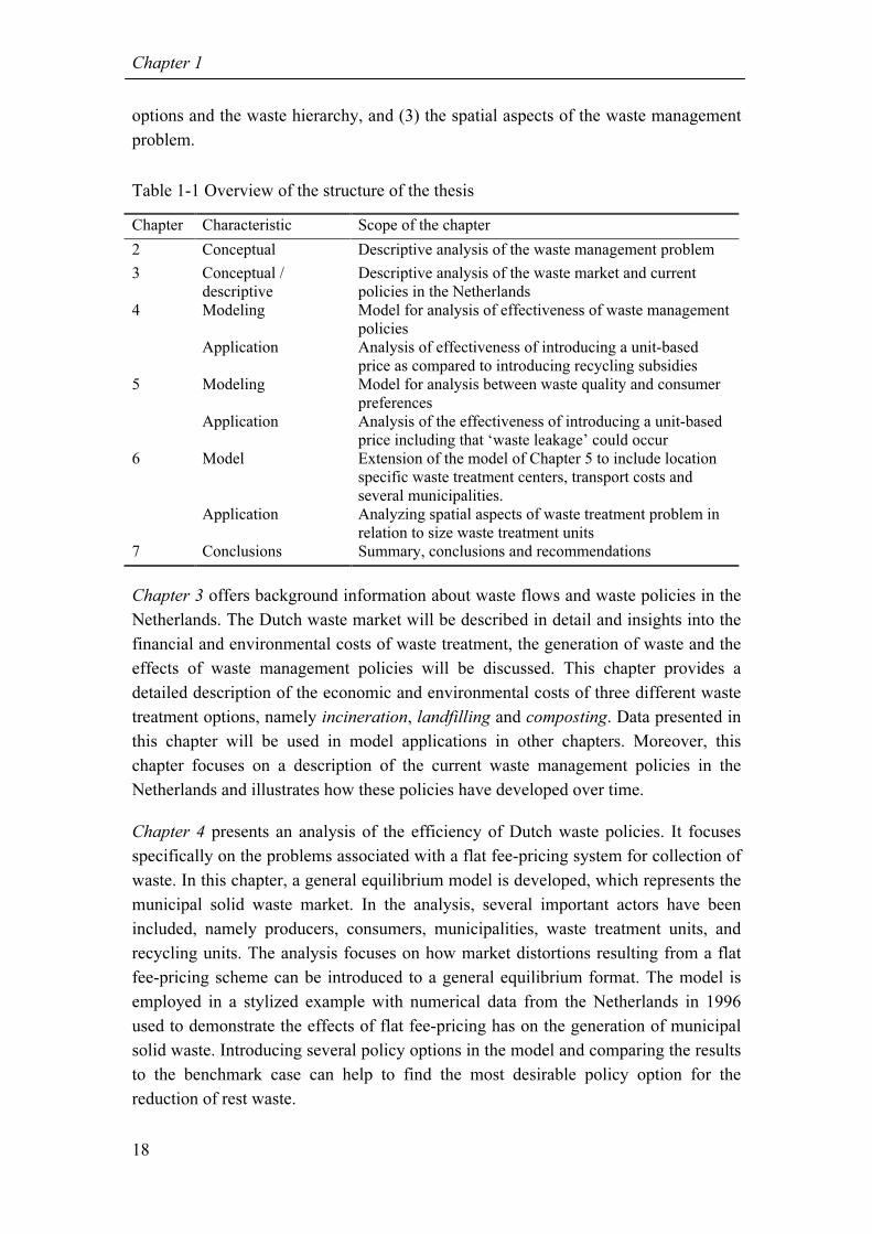
may thus necessarily be repeated in Chapters 4, 5 and 6. Table 1-1 gives a short
overview of the characteristics and scope of each chapter.
Chapter 2 provides a general overview of the municipal solid waste management
problem. Particular attention is paid to (1) several market distortions, which cause
waste generation to be inefficiently high, (2) the choice between waste treatment
Chapter 1
18
options and the waste hierarchy, and (3) the spatial aspects of the waste management
problem.
Table 1-1 Overview of the structure of the thesis
Chapter Characteristic Scope of the chapter
2 Conceptual Descriptive analysis of the waste management problem
3 Conceptual /
descriptive
Descriptive analysis of the waste market and current
policies in the Netherlands
4 Modeling
Application
Model for analysis of effectiveness of waste management
policies
Analysis of effectiveness of introducing a unit-based
price as compared to introducing recycling subsidies
5 Modeling
Application
Model for analysis between waste quality and consumer
preferences
Analysis of the effectiveness of introducing a unit-based
price including that ‘waste leakage’ could occur
6 Model
Application
Extension of the model of Chapter 5 to include location
specific waste treatment centers, transport costs and
several municipalities.
Analyzing spatial aspects of waste treatment problem in
relation to size waste treatment units
7 Conclusions Summary, conclusions and recommendations
Chapter 3 offers background information about waste flows and waste policies in the
Netherlands. The Dutch waste market will be described in detail and insights into the
financial and environmental costs of waste treatment, the generation of waste and the
effects of waste management policies will be discussed. This chapter provides a
detailed description of the economic and environmental costs of three different waste
treatment options, namely incineration, landfilling and composting. Data presented in
this chapter will be used in model applications in other chapters. Moreover, this
chapter focuses on a description of the current waste management policies in the
Netherlands and illustrates how these policies have developed over time.
Chapter 4 presents an analysis of the efficiency of Dutch waste policies. It focuses
specifically on the problems associated with a flat fee-pricing system for collection of
waste. In this chapter, a general equilibrium model is developed, which represents the
municipal solid waste market. In the analysis, several important actors have been
included, namely producers, consumers, municipalities, waste treatment units, and
recycling units. The analysis focuses on how market distortions resulting from a flat
fee-pricing scheme can be introduced to a general equilibrium format. The model is
employed in a stylized example with numerical data from the Netherlands in 1996
used to demonstrate the effects of flat fee-pricing has on the generation of municipal
solid waste. Introducing several policy options in the model and comparing the results
to the benchmark case can help to find the most desirable policy option for the
reduction of rest waste.

General introduction
19
In Chapter 5 a more detailed analysis of the interactions between the consumption
sector and the waste treatment sector is presented. In this chapter, the focus is on the
effectiveness of introducing a unit–based fee for the collection of municipal solid
waste. Introducing such a fee may lead to a reduction in waste generation but it may
also lead to an undesirable impact on the environment. Such a fee provides
households with incentives to generate lower quality organic waste as a form of
dumping. An applied general equilibrium model is presented that incorporates low
quality organic waste, high quality organic waste, and rest waste, and includes the
possibility of substitution between the generation of these three types of waste. The
model is used to analyze the effectiveness of introducing a unit-based pricing scheme
as compared to a flat fee-pricing system.
In Chapter 6, the model described in Chapter 5 is extended to include some important
spatial aspects of the waste management problem, in particular the location of the
waste treatment facilities in relation to transport costs and economies of scale. The
model includes several municipalities. Each municipality has the choice of
transporting their waste to a small, medium or large waste treatment facility. The
model includes transport costs and economies of scale for different sizes of waste
treatment facilities. The model also demonstrates that low quality waste can be
expensive to treat, thus showing the direct disadvantages of waste leakage. This
model is applied in a numerical example with data collected from the Randstad area in
2000. By extending the basic model of Chapter 5, a more extensive analysis can be
given about the effectiveness of introducing a unit-based pricing scheme as compared
to a flat fee-pricing system.
Chapter 7 contains the summary and main conclusions of this thesis. The five
research questions will be answered in this chapter. Finally, policy recommendations
and recommendations for future research are also given.

Chapter 1
20

21
2 Economics of waste management: key problems
2.1 Introduction
The increasing scale of economic activity, i.e. industrialization, urbanization, rising
living standards and population growth, has inevitably led to a sharp increase in the
total quantity of waste generated in our society. This large and increasing mass of
redundant goods, by-products, and organic and inorganic residue must be dealt with in
one way or another. The environment has a certain capacity for assimilation of waste,
but this capacity is not infinite. If too much waste enters the environment rather than
being recycled or re-used, the assimilative capacity of the environment is put under
too much stress and this results in pollution, resource degradation, and economic
damage (Turner, 1995).
In the Netherlands, the quantity of waste generated increased sharply due to the rise in
population growth and welfare throughout the last century. The quantity of municipal
solid waste generated has been steadily increasing since the beginning of the 20th
century. During the sixties and seventies, there was a sharp increase in income, which
resulted in a substantial rise in waste generation. Since the eighties, a proportional
relationship between the gross domestic product and the quantity of municipal solid
waste generated has emerged. This is illustrated in Figure 2-1.
90
100
110
120
130
140
150
160
170
1985 1987 1989 1991 1993 1995 1997 1999 2001
Index:
1985=100
Municipal solid
waste
Gross Domestic
Product
Total waste
production
Figure 2-1 The development of the gross domestic product and the production of
waste in the Netherlands, 1985-2001.

Chapter 2
22
Figure 2-1 reveals a decoupling of the growth of the gross domestic product and the
growth of total waste generation. This is mostly due to the steady increase of
recycling in several production sectors. In the construction and demolition sector, for
example, a recycling rate of 94% has been achieved. The growth rate of municipal
solid waste generation is still linked to the growth rate of the gross domestic product.
Although policy makers aimed to decouple income and waste generation, they have
failed to achieve this for this particular waste stream.
Economic growth has led to an enormous increase in economic welfare. Material
wealth has increased significantly and the quantity of goods available to the consumer
has grown sharply. Due to the laws of thermodynamics, economic production and
consumption always generate some pollution and waste. It is not possible to recycle
for a full 100%. A society, however, can to some extent choose how much waste it
generates through prevention, re-use, or recycling. By subsidizing recycling or by
taxing landfilling, for example, the government can influence the quantity of waste
generated. To design an efficient management plan, the government must balance the
social benefits of a particular economic activity with the social costs (including
disposal) related to this activity.
Waste treatment, such as composting, incineration, and landfilling, creates many
problems for our society. It is costly to treat waste. For example, it leads to
environmental problems and takes up valuable space. Available evidence shows that
industrial countries are trying to cope with an increasing number of problems caused
by disposal of waste. To build a waste treatment unit, a site has to be found that is
technically suitable, i.e. the right soil and not too expensive, and socially acceptable.
Some countries, such as the USA, Germany, and the Netherlands have a shortage
(either locally or nationally) of sites that are technically suitable for building landfill
or incineration units. This means that even if it is sociably acceptable to build a
landfill or incineration unit, there simply is not enough space available to construct
one. In other industrial countries there may be enough sites available, which are
technically suitable for building an incineration or landfill site, but in these countries
there is a shortage of possible landfill and incineration sites that are socially
acceptable. The NIMBY (Not In My Back Yard)-syndrome plays an important role in
the process of deciding on a possible disposal site (Turner, 1995).
National policy makers in the EU face an additional problem because the European
Commission and Council have decreed that the ‘proximity principle’ should be an
accepted part of all members states waste management policy. According to the
proximity principle, ‘provisions must be made to ensure that as far as possible waste
is disposed of in the nearest suitable waste treatment centers’. Thus, the export is not
permitted, as it would place an unfair burden on the environment of the importing
country (see for more information Monkhouse and Farmer, 2003). The proximity
principle only applies to waste that must be incinerated or landfilled. Recyclable

Economics of waste management: key problems
23
waste can be exported if adequate proof is given that the importing country is actually
going to recycle the imported waste.
The municipal solid waste problem is still relatively new and policymakers are trying
to cope with it in the best way possible. Considerable research has already been
conducted on this topic. This chapter surveys the literature on the major questions and
theories in the area of municipal solid waste management:
• How should the municipal solid waste market be regulated to reduce the generation
of municipal solid waste?
• What is the optimal mix of waste treatment options?
• Where should waste disposal units be located, considering social, political, and
economic preferences as well as pure technical aspects?
Section 2.2 discusses the optimal regulation of the municipal solid waste market and
inefficiencies that are present in the current municipal solid waste market. Section 2.3
deals with the question of whether there is an optimal waste treatment method.
Section 2.4 looks at ways of determining the optimal location of a waste disposal unit.
Finally, Section 2.5 concludes the chapter.
2.2 Waste generation: the optimal policy mix
One of the most fundamental questions regarding the waste management problem
concerns the ‘optimal’ quantity of waste that a society should generate. Most
environmental scientists argue that we should not generate waste at all. Natural cycles
like, for example, the hydrological cycle or the carbon cycle are closed, which means
that waste generated during these cycles will be re-used as inputs. The industrial cycle
should be fashioned after the natural cycle, thus we should try to close the material
cycle and re-use or recycle all materials we consume. This idea of ‘treating the
economy as a living organism’ is called industrial metabolism (Anderberg, 1998;
Ayres and Simonis, 1994). Presently, our society is nowhere near to closing the
industrial cycle. This cycle still extracts high-quality materials, such as fossil fuels
and ores, from the earth and returns them to the earth in degraded forms; it only re-
uses part of its waste.
From an economic point of view, it may not be necessary to fully close the material
cycle. It is often forgotten that both recycling and re-use of materials have financial
and environmental impacts, which makes it undesirable to completely eliminate waste
generation (Pearce and Turner, 1993). Both environmental scientists and
environmental economists, however, agree that too much waste is currently being
generated (see for example Graig, 2001). The question remains just how much waste

Chapter 2
24
should be generated and how the waste market can be regulated to produce the
‘optimal’ quantity of waste. Fricker (2003) argues that the only sustainable way of
reducing waste generation is by reducing consumption. The majority of
environmental economists, however, do not share this view. In the next section, a
number of policy instruments, which can be used to control waste generation, will be
discussed.
2.2.1 Waste generation and the pricing mechanism
Waste management in most countries is still dominated by inefficient pricing,
institutional and legal structures. The primary virtue of the pricing mechanism, i.e. the
market, is that it gives consumers an idea of the costs of producing a particular
product and offers producers insight into how consumers value a product (Löfgren,
1995). Naturally, the pricing mechanism only supplies the correct information if the
market is undistorted. Solid waste management pricing is mostly based on a flat fee
system. Households pay a fixed charge, the so-called flat fee, for the collection of
waste. The amount of the fee is independent of the quantity of waste that is actually
generated, thus consumers have no price-incentive to reduce the generation of waste,
and thus larger quantities of waste are disposed of than is socially desirable.
Figure 2-2 illustrates the demand curve for waste collection services1. As the price of
these services declines, the demand for these services increases. In the case of
household waste disposal, the price of disposing one extra unit of waste equals zero,
as the price is independent of the quantity of waste disposed of.
b
c
Price
SWS
P*
Q0Q*
a
Figure 2-2 The demand curve for solid waste services (SWS)
Source: Jenkins (1993)
1 The demand curve shown in Figure 2-2 is just an illustration of a possible demand curve. In reality, it
may well be that the demand for solid waste services is not linearly related to the price of these
services.

Economics of waste management: key problems
25
The quantity of waste disposal services demanded is equal to Q0 and so consumption
in terms of disposal costs is not restrained. If the price, i.e. the marginal costs of waste
disposal, is equal to zero then Q0 will be the optimal quantity of waste disposal. If,
however, the marginal costs of waste disposal are positive, the demand for solid waste
services is clearly higher than optimal. Assume, for example, that the social costs of
waste disposal are equal to P*, then the optimal demand for solid waste services will
be equal to Q*. Society faces a net total cost equal to the triangle abc caused by the
inefficiently high demand for waste disposal services. Only when the disposal fee is
equal to the exact marginal costs of waste disposal will the demand for waste disposal
services equal the optimal quantity of waste disposal (Jenkins, 1993).
Finding the optimal disposal fee, however, poses several problems. The optimal
disposal fee should cover both the marginal financial and the marginal environmental
costs of municipal solid waste disposal and treatment. It is, therefore, important to
quantify all external effects caused by waste treatment. However, as Figure 2-2
clearly demonstrates, the flat fee-pricing scheme will always lead to a non-optimal
quantity of waste generation since the marginal costs of waste disposal are most
assuredly positive.
It is important to note that the flat fee and the quantity of waste generated are not
unrelated. The flat fee is determined by the quantity of waste generated in previous
years. The flat fee will completely or partly cover the costs of collection and treatment
of municipal solid waste. The flat fee, however, will not provide households with an
incentive to reduce waste generation, as the marginal price of waste generation equals
zero.
2.2.2 Finding the optimal policy mix
A lot of research has been done to determine the optimal policy mix to both stimulate
consumers to generate less rest waste as well as to encourage more recycling and
composting. The findings of these studies are discussed below using a simple general
equilibrium model built by Kinnaman and Fullerton (1999).
In the model developed by Kinnaman and Fullerton, n identical households are
distinguished. Each of these households maximizes utility (u) over consumption (c).
Consumption generates waste and this waste must either be disposed of as waste (g)
or be recycled (r). The function c(g,r) represents all possible combinations of waste
and recycling given a certain level of consumption. Consumer i maximizes utility
given the price of consumption (pc), the price of garbage disposal (pg), the price
received for recycled materials (pr) and the available income (y).
[ ( , )] 1,...,i i i i i
Max u u c g r i n= = (2.1)

Chapter 2
26
Subject to the budget constraint:
( , )c g r
i i i i i iy p c g r p g p r= + − (2.2)
According to this model, the production sector produces the consumption good with
the input of virgin material (v) and recycled material (r). The production function f
represents the production possibility set of the producer. He maximizes profits (π)
given the prices pv en pr:
( , )c v rMax p f v r p v p rπ = − − (2.3)
In the equilibrium solution, consumers will choose optimal levels of recycling and
waste disposal. All recycled material is used by the production sector and the
producers choose an optimal mix between using virgin material and recycled material.
In this simple model, the external effects created by waste disposal are disregarded,
which is not a realistic assumption. Disposal leads to many environmental
externalities, such as the pollution of ground water and emissions that contribute to
the problem of climate change, acidification and other environmental problems.
Assume that household utility is influenced by the total quantity of waste generated in
society: ui = ui(c,G) where uG < 0 and G=ng. The solution found by the model
described in equation 2.1 to 2.3 does not represent the optimal levels of recycling and
disposal. For a positive G, u(c,G) will always be lower than u(c). If consumers fail to
internalize the social external costs of waste treatment in their utility function, the
calculated levels of recycling will be too low and the level of waste disposal will be
too high.
To internalize the external costs created by waste treatment in the price of waste
disposal, economists have proposed the use of several taxation or subsidy schemes.
To stimulate household recycling, the government may choose to tax waste disposal
(at rate tg), subsidize recycling efforts of households (at rate shr), or impose an
advanced waste disposal fee at the time of purchase (at rate tc). The maximization
problem for the individual household is thus defined as:
[ ( , ), ]i i i i i
Max u u c g r G= (2.4)
Subject to the budget constraint:
( ) ( , ) ( ) ( )c c g g r hr
i i i i i iy p t c g r p t g p s r= + + + − + (2.5)
To directly stimulate the use of recycled materials the government can choose to tax
the use of virgin materials (at rate tv) or subsidize the use of recycled materials (at rate
s f r ).
Economics of waste management: key problems
27
The profit maximization problem transfers into:
( , ) ( ) ( )c v v r f rMax p f v r p t v p s rπ = − + − + (2.6)
Levying a tax (tg) on the generation of waste is the most direct approach to internalize
the external costs of waste disposal. Most municipalities in the Netherlands and other
countries throughout the world charge a flat fee for the collection of waste, either
through local property or income taxes. This means that the marginal private costs of
generating municipal solid waste (pg+tg) equal zero whereas the marginal social costs
of generating municipal solid waste are positive. The introduction of a positive tax tg
can induce households to internalize the social costs of waste disposal in their
decisions about generating waste.
Wertz (1976) was the first to estimate the effects of a unit-based price for municipal
solid waste by comparing data from a municipality in the USA, which charged a user
price for the collection of waste, with data from the rest of the USA that was
representative of municipalities, which charged flat fees, for the year 1970. His results
suggest that the introduction of user prices reduces the generation of municipal solid
waste.
On the basis of panel data from 12 cities in the United States, Jenkins (1993)
estimated that introducing a unit-based pricing could reduce the social costs of waste
treatment by about $125 per tonne of waste. This would improve social welfare by
$650 million a year, roughly $3 per person per year. Fullerton and Kinnaman (1994)
estimated similar welfare increases by analyzing the effects of the introduction of a
volume-based pricing system in Charlottesville, Virginia. Podolsky and Spiegel
(1998) calculated the largest social welfare increase. They estimated that the
introduction of a unit-based pricing resulted in social welfare benefits of $12.80 per
person based on an analysis of cross-section data from a town in New Jersey (USA).
One advantage of the unit-based pricing system is that it is directly based on the
‘polluter pays principle’ as established in the framework directive on waste of the
European Union, which, among other things, rules that the cost of waste disposal
should be borne by the individual who generates it. The ‘polluter pays principle’ is
generally accepted as instrument of justice given that it not only charges the polluter
for the administrative and environmental costs generated by their behavior, but it also
encourages the polluter to mend his ways (Perman et al., 1996). Goddard (1995),
however, raises an interesting question regarding the ‘polluter pays principle’ namely,
who is the actual polluter in this case? Is it the consumer who generates the waste by
consuming the product, is it the producer who designs a product that contains either
too much waste or is not recyclable, is it the package designer, who pays little
attention to the waste content of his design, or is it the retailer who desires packaging
that keep transaction costs low? It is impossible to answer this question. Goddard

Chapter 2
28
demonstrates that it is more appropriate to consider which of the actors is in the best
position to control the waste flow. A well-informed consumer would be the proper
person to make personal consumption choices. By getting the prices of waste disposal
right, the consumers can decide on their own how much municipal solid waste should
be prevented or recycled.
Another advantage of the unit-based price is that it ensures an efficient allocation of
resources without requiring the other tax and subsidy instruments mentioned above
(Fullerton and Wu, 1997 and Palmer and Walls, 1994). If a unit-based price is
introduced, households will start to consume, recycle, and dispose waste in such a
way that the marginal benefits of consumption and recycling are equal to the marginal
costs of disposal. In such a case, the market will provide the proper prices for
consumer goods, recycling and disposal. For example, if consumers start to recycle
more waste, recycled material becomes cheaper. Thus producers will start to use more
recycled material without needing an extra incentive of the government in terms of a
recycling subsidy (Kinnaman and Fullerton, 1999). In fact, Dinan (1993) shows that
introducing both a unit-based price on waste disposal and a subsidy on the use of
recycled material is inefficient as this basically subsidizes the use of recycled material
twice.
Several studies, however, have illustrated that the introduction of a unit-base price
will lead to significant transaction costs, thus it may be inefficient to introduce such a
pricing system. First of all, the administrative costs of introducing a unit-based price
may exceed the social benefits of lower waste generation. Fullerton and Kinnaman
(1996) estimate that the administrative costs of introducing a unit-based price on the
bases of an ‘expensive bag’ in Charlottesville, Virginia could exceed the $3 per
person social benefits mentioned before. Linderhof et al. (2001), however, reveal that
in Oostzaan the cost of waste collection and disposal did not increase after the
introduction of a weight-based price for waste collection. Furthermore, they show that
the costs invested in the introduction of the weight-based pricing system are
compensated by the lower cost of waste treatment due to the reduction of waste.
These results depend largely on the individual municipality. In the case of Linderhof
et al., the average consumer in the municipality was very environmentally friendly
oriented. Thus, consumers were more than willing to recycle and prevent waste. It can
be expected that results in other municipalities would be less positive.
Secondly, Dinan (1993) showed that a uniform unit-based price for all types of waste
might be inefficient if materials within the waste stream led to different social costs.
For example, the treatment of hazardous waste, such as flashlight batteries, will
generate far greater social costs than the treatment of recyclable waste, such as old
newspapers. The unit-based price collection of flashlight batteries should, therefore,
be higher than the unit-based price for collection of old newspapers. Other studies,
such as Walls and Palmer (2001), Eichner and Pethig (2001), and Calcott and Walls

Economics of waste management: key problems
29
(2002), support these results. A solution would be a selective unit-based pricing
system based on the social costs of disposing the material in question, this would of
course be rather expensive to implement.
Thirdly and most seriously, the unit-based pricing system may promote the illegal
disposal of waste. Households may start to dump their waste in their neighbors’ bins,
dispose of it at work, illegally dump waste, or burn it themselves. Such behavior leads
to large social costs and has been identified as one of the most serious obstacles to the
introduction of a unit-based pricing for waste collection. Both Dobbs (1991) and
Fullerton and Kinnaman (1995) demonstrate that if illegal disposal is a possibility, it
may be optimal to have a negative tax on waste disposal, i.e. legal waste disposal
should be subsidized. In such a case, policy makers would be better off implementing
other policy instruments to reduce waste generation. Fullerton and Kinnaman (1996)
estimate that about 28% of the decrease in waste generation may be caused by
increased illegal disposal. Empirical studies, like Jenkins (1993) and Miranda and
Aldy (1998), also report instances of increased illegal dumping. These results,
however, are contradicted by other empirical studies. For example, Miranda et al.
(1994), Strahman et al. (1995), Nestor and Podolsky (1998), Podolsky and Spiegel
(1998), Sterner and Bartelings (1999) and Linderhof et al. (2001) found no significant
evidence of increased illegal disposal.
Despite the three disadvantages mentioned above, the unit-based price is one of the
most effective policy options to provide an incentive to increase prevention and home
composting. None of the other policy tools can significantly influence the consumers’
choice to prevent waste. Therefore, Calcott and Walls (2002) find that a modest
disposal charge will always be part of the set of optimal policy instruments. Shinkuma
(2003) even goes a little farther, arguing that even if illegal disposal is an option, the
unit-based pricing system will still provide a second best optimum as long as the price
of recycled material is positive. Only if the price of recycled material is negative,
should another policy tool like the deposit-refund system be considered.
As mentioned above, the unit-based price alone may not provide an efficient solution
to the municipal solid waste problem and it may be necessary to use other policy
instruments. Miedema (1983) was one of the first to evaluate the potential use of other
policy instruments. He found that the introduction of a tax on the use of virgin
materials (tv) provides more welfare gains than a subsidy on the use of recycled
materials (sfr), a unit-based price for waste collection (tg) or an advantaged disposal
fee internalized waste disposal costs in the price of a product (tc). Although both the
unit-based pricing scheme and the advantaged disposal fee can reduce waste
generation and increase recycling, the necessary fee must be high, which can
stimulate illegal disposal. Besides the transaction costs of introducing these systems
and the social costs of disposal are too great to be cost-efficient. A tax on the use of
virgin materials provides an incentive to use fewer virgin materials and at the same

Chapter 2
30
time boost the market for recycled materials. Miedema thus favors the virgin material
tax above other policy instruments.
Pearce and Turner (1993) conclude that both virgin material taxes and unit-based
pricing could indeed be used to correct market distortions in the waste market. A later
study by Bruvoll (1998) supports the conclusion that the introduction of a virgin
material tax will result in significantly higher use of recycled materials and lower
quantities of waste generated thus considerably reducing social costs of waste
disposal. Moreover, taxing virgin material may be an efficient tool for reducing air
emissions, thus reducing social costs of using virgin materials.
Conrad (1999) demonstrates that a virgin material tax provides firms with a strong
incentive to reduce waste generation; a much stronger incentive than the unit-based
price provides. Not all studies agree with this result. For example, Dinan (1993)
shows that only those producers who are able to substitute virgin material for recycled
material will do so. This means that a large number of industries that have no real
option to substitute virgin material will not be induced to use more recycled material
at all, thus the demand for recycled materials will not be affected as much as could be
expected. Furthermore, a local virgin material tax will not affect the export of
recycled materials. Since a large part of recycled materials, like paper and plastic, are
exported to the United States, the virgin material tax will be less effective.
Palmer and Walls (1994) demonstrate that a virgin material tax indeed encourages the
use of recycled materials, but that it also discourages production and consumption.
Thus the social costs of a virgin material tax are too high to be efficient. Not all
studies, however, agree on the macro-economic effects of a virgin material tax.
Bruvoll et al. (1999) show that the improvement in environmental quality caused by
increased recycling could increase productivity and in turn curb the decline in
production and consumption. Fullerton and Kinnaman (1995) conclude that the
introduction of a virgin material tax is only useful in addressing the environmental
problems caused by extraction of virgin materials (strip mining) and cannot be used to
tackle the environmental problems caused by waste generation. Palmer and Walls
(1997) share the same opinion. They advocate that the deposit-refund system is a
more useful policy instrument.
Besides taxing virgin material, the use of recycled material can be stimulated by
subsidizing recycling. The use of a recycling subsidy has been extensively researched.
Fullerton and Wu (1998) argue that if unit-based prices cannot be implemented due to
risk of illegal disposal, recycling subsidies aimed at the firm (sfr) can indeed improve
welfare and should be chosen as the preferred tool to minimize the social costs of
waste disposal. Palmer and Walls (1994) find that recycling subsidies for both firms
and households (sfr en shr) supply a more optimal mix between waste generation and
recycling. If, however, a recycling subsidy would be the sole instrument to be

Economics of waste management: key problems
31
implemented it could excessively stimulate both production and consumption, and
thus waste generation. They advocate that it would be better to introduce a recycling
subsidy combined with a consumption tax (tc). Only this combination may induce
consumers to recycle more and reduce waste generation (Palmer et al., 1997). This
subsidy/tax system is similar to a deposit refund system.
Other studies have also identified the deposit-refund system as the optimal policy
instrument to reduce waste generation and increase recycling. With the help of a
general equilibrium model, Fullerton and Kinnaman (1995) illustrate how a deposit-
refund system could significantly reduce social waste disposal costs and that it should
be implemented as the preferred policy instrument whenever illegal waste disposal is
a serious option. Palmer et al. (1997) show that the introduction of a deposit-refund
system would have effectively reduced waste generation by 7.5% in 1990, thus
resulting in a social welfare benefit of $33 per tonne of waste. Other economic
studies, like Dobbs (1991), Dinan (1993), Palmer and Walls (1994), and Atri and
Schellberg (1995) favor the use of a deposit/refund system.
In the optimal deposit/refund system the deposit equals the marginal social costs of
waste disposal. The refund is equal to the social waste disposal costs minus the
marginal social costs of recycling. If the marginal social costs of recycling equal zero,
the refund matches the deposit exactly. The deposit can be levied on either the
production or the sales of a product and the refund can be given to either the producer
or the consumer. If the refund is returned to the consumer, the consumer has a direct
incentive to increase recycling. This increase in recycled materials will in turn drive
the price of recycling down. Thus the demand for recycled material will increase. If
the refund is given to the firms, the firms will start to demand more recycled material,
this will increase the price of recycled materials thus giving the consumers an
incentive to recycle more (Atri and Schelberg, 1995). In addition, both Fullerton and
Wu (1998) and Eichner and Pethig (2001) demonstrate that the deposit/refund
provides an incentive to change the design of the product to improve its recyclability.
High transaction costs are the greatest disadvantage of the deposit/refund system. The
most optimal deposit/refund system would be a differentiated system for various
materials. This system, however, is also the most expensive. Palmer et al. (1995)
calculate that the marginal costs of reducing waste by 10 percent are equal to $45 per
tonne waste reduced. In comparison, the marginal cost of reducing waste by 10
percent with the use of a recycling subsidy would be equal to $98 per tonne of waste.
These marginal costs, however, do not include the administrative costs of
implementing the system. If these costs are included, the marginal costs of the
deposit/refund system will increase sharply. However, Palmer et al. find that in the
case of California the marginal costs including the administrative cost of a
deposit/refund system are still expected to be lower than the marginal costs including

Chapter 2
32
administrative costs of a recycling subsidy, thus showing that the deposit/refund
system is more cost-efficient than the recycling subsidy.
Dinan (1993) asserts that if the costs of introducing a deposit/refund system are high,
the government should select those waste materials, which either cause a large part of
the municipal solid waste stream, like old newspapers, or of which disposal causes
large social costs, like flashlight batteries. Fullerton and Wolverton (2000), however,
point out that it is not necessary that the deposit and the refund are exactly equal to
each other, nor is it necessary that the deposit and the refund are placed on the same
actors in the market place. Thus, as suggested by Palmer et al. (1995), the deposit-
refund may be placed upstream to avoid dealing with private households,
consequently avoiding substantial transaction costs. Calcott and Walls (2002) support
these results. They show that in a system where the producers of goods that are
recycled pay a tax-upfront, which equals the refund received by recyclers, and the
producers of goods that are not recycled pay an advanced disposal fee, which equals
the marginal costs of treatment, can indeed provide a second-best equilibrium
solution.
Besides tax and subsidy instruments, the government also has command and control
policies at its disposal. Most of the command and control options are aimed at
promoting waste recycling. The three most popular command and control policy tools
in both the United States and the European Union are: 1) Product specific minimum
content standards, 2) Material specific utilization requirements and 3) Producer
responsibility (Goddard, 1995).
1) The product specific minimum content standards specify the minimum quantity of
recovered materials that a product must contain. Materials most commonly mentioned
are aluminum, steel, glass, and paper used in packaging. The product specific
minimum content standards have been applied in various parts of the United States
and various countries in the European Union. Although widely applied, little research
has been done to examine the effectiveness of the minimum content standards. One
exception is the research conducted by Palmer and Walls (1997). In this study, Palmer
and Walls evaluate the effectiveness of minimum content standards as compared to
taxes and subsidies. They find that while the material content standard can lead to
lower output of municipal solid waste, it can also lead to inefficient use of other
production factors such as labor. To negate these unintentional effects, it may be
necessary to implement additional taxes and subsidies. Moreover, to set efficient
standards, extensive knowledge about the production function of a firm is necessary.
This information is not always available. If industries are heterogeneous, setting a
uniform, optimal standard may be impossible.
2) The material specific utilization requirements specifies that producers must recover
and use a certain predefined percentage of specific materials, like packaging and non-
Economics of waste management: key problems
33
durable goods, that normally would be disposed of. Materials that are normally used
are paper, glass, aluminum, steel, and plastic. New Jersey, for example, passed a law
in 1987 that 25% of all waste had to be recycled. Municipalities were forced to
develop and submit a recycling plan as part of their solid waste plans. The law stated
that three materials had to be recycled; the municipalities were allowed to choose
which three materials. Most municipalities chose paper, aluminum, and glass since
these materials take up a large part of the typical household waste stream. The law
was indeed effective and after two years the state of New Jersey was well on its way
to realizing the 25% recycling rate (Callan and Thomas, 1996).
3) The producer responsibility specifies that producers of goods ultimately destined
for disposal directly responsible for the collection, recycling, the disposal, and the
associated financial and external costs. Walls (2003) demonstrates how difficult it is
for the government to design and implement cost-effective environmental policies to
spur producer responsibility. She warns of the danger that the costs of introducing
producer responsibility may outweigh the benefits of such a system. Runkel (2002)
shows how producer responsibility can influence both durability and welfare. He
argues that under perfect competition, the producer responsibility can achieve a first-
best equilibrium solution. Even if no perfect competition exists, the producer
responsibility will raise welfare as compared to a situation where producers do not
receive a price incentive to limit waste disposal.
Germany was the first country to introduce a far-reaching producer responsibility
program in 1991. This program, which is known as the ‘green dot’ program, sets
extensive recycling targets for several materials, such as glass, paper, aluminum, and
plastic, and aims to achieve these targets by making the industry directly responsible
for the collection and recycling of all its packaging. The industry responded to these
regulations by forming a private non-profit company Duales System Deutschland,
which provides collection and recycling services for consumers. The DSD system
sells participating companies the right to put a green dot on their product, a symbol,
which guarantees that the packaging of the product is eligible for the services
provided by the DSD. The program has been a huge success in terms of recycling
efforts, but it has not been without problems. The costs of the program are quite high
and the system of the green dot is prone to fraudulent activities (Goddard, 1995). The
large increase in recycling rates, however, has stimulated various countries such as the
Netherlands, France, the United States, and Japan to implement producer
responsibility programs of their own. For an extensive overview of the
implementation of producer responsibility programs in other countries see Palmer and
Walls (2002).
This section has provided a concise overview of the literature dealing with policy
instruments to control the problem of municipal solid waste management. As should
be clear, there is no unique solution to policy questions regarding the municipal solid

Chapter 2
34
waste problem. Most of the studies agree that without the possibility of illegal
disposal, the unit-based pricing scheme for collection of waste is the preferred policy
instrument. If illegal disposal is a serious threat, most of the studies favor a
deposit/refund system.
2.2.3 Elasticities of the demand for waste disposal services and consumer attitudes
towards recycling
The success of market based policy instruments, like the ones mentioned in Section
2.2.2, depends on the elasticity of demand for waste disposal services. For example, a
unit-based price for waste disposal will only affect the disposal of waste if the demand
for disposal services is sensitive to the price of the waste disposal services. As
municipalities have been experimenting with the introduction of recycling programs,
unit-based pricing, and deposit/refund systems, a large range of empirical studies
discussing the price elasticity of waste generation have been conducted. In this
section, I will discuss the most important literature on this subject.
Wertz (1976) analyzed the households’ responsiveness to unit-based prices. By
comparing the average quantity of waste generated in San Francisco, a city with a
user fee, with the average quantity generated by an average town of the United states,
without a user fee, Wertz calculated a price elasticity of demand equal to –0.15.
Hong et al. (1993) examined the effects of volume-based pricing using a survey of
2298 households from Portland OR, USA. Hong et al. estimated a price elasticity of
demand equal to –0.03 and an income elasticity of 0.049 suggesting that unit-based
pricing only affects demand in a minimal way. They did, however, find that the
demand for recycling services is influenced positively by the introduction of volume-
based pricing. They also concluded that households are less likely to increase
recycling if recycling requires more effort and that a larger household is not only
more likely to recycle, but also to generate more waste than a smaller household.
Jenkins (1993) gathered data from 14 municipalities in the United States (including 10
municipalities that charged a unit-based price) over several years. She found an
inelastic demand for waste disposal, reporting a price elasticity of –0.12. Jenkins
concluded that waste generation and recycling is positively influenced by the size of
the household. However, she also found the effect to be statistically insignificant.
Miranda et al. (1994) used data from a 21-city sample to estimate the effects of
introducing a unit-based price. They found that unit-based pricing provides residents
with a strong incentive to both reduce waste and recycle it. They note, however, that
most municipalities implement a unit-based price in combination with an aggressive
recycling program. In the one municipality that introduced unit-base pricing on its
own, the experiment failed. Households turned to private waste collectors and illegal

Economics of waste management: key problems
35
disposal increased significantly. Therefore, this municipality chose to return to the flat
fee-pricing system. This evidence, although anecdotal, seems to suggest that a unit-
based pricing scheme cannot be successful without a recycling program.
Morris and Holthausen (1994) use a household production model to simulate
responses to different pricing systems using calibration techniques. They estimate that
the elasticity of demand for waste disposal services was in the range of –0.51 and
-0.6.
Reschovsky and Stone (1994) employed an econometric model to estimate the actual
household responses to unit-based pricing. They used data from 3040 households
from Tompkins Country, New York. Based on these data, they estimated income
elasticities for the demand of collection services equal to 0.23 in case of the
introduction of volume-based pricing and 0.24 in case of the introduction of weight-
based pricing. These results are quite similar to the results found by Wertz (1976).
Reschovsky and Stone try to determine how much waste was illegally disposed of.
They found that much of the illegal dumping takes place in the form of the use of
alternative dumping facilities, such as roadside dumpsters. They were unable to
determine how often illegal dumping or burning occurred. They argued that
households are not quite as sensitive to the increased marginal costs of waste disposal
as they are to the increased marginal costs of waste reduction. Thus households will
only try to reduce waste generation if the marginal costs of waste reduction do not
increase too greatly. If the marginal costs of waste reduction increase too much,
households will dump waste illegally to reduce the costs of waste disposal. These
results suggest that households may have an aversion towards the introduction of a
unit-based pricing, indicating that municipalities would be wise to combine a unit-
based price with recycling programs or subsidies. Introducing a unit-based price
without such a program would be unpopular and less effective.
Strathman et al. (1995) estimated the price elasticity of demand for solid waste
disposal services using data from Portland, Oregon. They used data on the generation
of waste during January 1984 to December 1991. They found an elasticity of demand
of –0.45. This elasticity is quite a bit lower than elasticities cited earlier. Strathman et
al. note that they may have overestimated the absolute elasticity as they expect that
the propensity of illegal disposal may be somewhat higher in the Portland region due
to the large amount of public land available in this area.
Fullerton and Kinnaman (1996) used household data that were not based on self-
reported surveys. They gathered data about the weight and volume of municipal solid
waste and recycling efforts of 75 households four weeks prior to, and following the
introduction of a volume-based price in Charlottesville, VA. In this municipality, a
recycling program had all ready been operational for about a year. They found that the
quantity of solid waste generated decreased only slightly, but that the volume of the

Chapter 2
36
waste collected decreased all the more. The density of the municipal solid waste
increased significantly, from 15 pounds per bag to just over 20 pounds per bag. They
estimated that the introduction of the unit-based price resulted in ten percent less
waste, four percent more illegal dumping, and 14 percent more recycling.
Callan and Thomas (1997) found that the implementation of a unit-based price would
increase the portion of waste recycled by 6.6 percent. If the introduction of a unit-
based price was combined with the introduction of a recycling program, the portion of
waste recycled would increase by 12.1 percent.
Kinnaman and Fullerton (2000) were the first to estimate both the levels of recycling
and the level of waste disposal simultaneously after the introduction of a unit-based
price. They estimate that the cross price elasticity of demand for recycling is 0.220.
Moreover, they not only found that an implementation of a $1 unit-based price can
decrease the quantity of rest waste generated by 415 pounds per person year, but that
it would only increase the quantity of recyclable waste by 30 pounds per person per
year. The difference can be partly explained by increased home composting and
prevention, but also points towards the increased illegal disposal of waste.
Although the calculated elasticity of the demand for waste disposal services differs
quite a lot between different studies, we can conclude that the demand for waste
disposal services is inelastic. The introduction of a unit-based price will result in a
reduction of waste. At least part of this reduction, however, may be caused by
increased illegal disposal of waste. It is difficult to give definite empirical proof of
increased illegal disposal. Although survey respondents claim that illegal disposal has
increased after the introduction of a unit-based price, municipalities have not reported
increased costs due to illegal dumping and littering.
The empirical studies discussed above report various elasticities of demand for waste
disposal services. These differences may be partly explained by differences in
attitudes of the households. Several empirical studies have analyzed why consumers
recycle or compost at home. In the next couple of paragraphs, a brief overview of
these studies is given. For a more extended overview, see Fenech (2002)
Several studies, for example, Hornik et al. (1995), McDonald and Ball (1998), Callan
and Thomas (1999), Bruvoll et al. (2000, 2002), Tucker and Speirs (2002), Ando and
Gosselin (2003) and Jenkins et al. (2003), have shown that the opportunity cost of
time is a significant determinant for recycling of materials. The more households have
to do to recycle and separate waste, the less willing they are to do so. A majority of
the consumers are willing to pay a private company about 20 dollars a year to take
away the burden of separating waste (Bruvoll et al., 2002). Jenkins et al. (2003)
conclude that consumers are more likely to recycle materials like aluminum, or paper

Economics of waste management: key problems
37
given that effort in recycling these materials is less than other materials such as glass,
plastic, and organic waste.
Recycling behavior is influenced by socio-economic factors such as income,
education, population density, single or multiple family dwellings, household size and
average age of the head of the household. Most empirical studies, like Jenkins et al.
(2003), find that income and education are positively correlated with recycling.
Population density is negatively correlated with recycling and specifically with home
composting of organic waste. An explanation for this correlation is the growing
scarcity of suitable outdoor storage of waste as the population density increases. Age
and household size have a positive correlation with recycling. Ando and Gosselin
(2003) show that multi-family dwellings are less likely to recycle than single-family
dwellings. They find that differences in recycling convenience and household
demographics are the main reason why this occurs.
Introducing a unit-based pricing system not only increases recycling of waste, but also
changes the attitude of households towards waste. Fullerton and Kinnaman (1996)
demonstrate that the introduction of a volume-based pricing system in Charlottesville,
USA did not so much decrease the quantity of waste generated, but instead decreased
the volume of the waste generated. Households reduced the number of bags they
generated by crushing the waste down in size, rather than by preventing or recycling
it. Households, however, were already participating in voluntary recycling programs
before the introduction of the volume-based price, thus the incremental benefit of the
volume-based price was low.
Sterner and Bartelings (1999) show that the introduction of a unit-based price in
Tvååker, a municipality in Sweden, led to a significant reduction of the quantity of
waste collected and that the quantity of waste recycled increased. With an extensive
survey of about 600 households and focusing on the motivation behind recycling, they
demonstrate that whilst people are encouraged by economic incentives, this is not the
only reason why they start to recycle. The amount of time and effort invested in
recycling are greater than can be purely motivated by savings on their waste
management bill. Halvorsen and Kipperberg (2003) support this conclusion. Berglund
(2003) analyses the effect of moral motives on household recycling. He finds that
moral motives significantly reduce the costs associated with recycling efforts, thus
consumers are more willing to recycle even when they are not financially
compensated for doing so.
2.3 The optimal mix of waste management methods
In the previous section, I have outlined the instruments policy makers have at their
disposal to reduce waste generation. Even if a society reduces waste generation as

Chapter 2
38
cost-efficiently as possible, it is likely that a substantial quantity of waste will still
have to be disposed of. In this section, I will, therefore, discuss how waste can be
treated and what kind of environmental problems waste treatment can cause.
The physical and thermal properties of various solid waste types, such as calorific
value, ash, moisture and bulk density, give a reasonable indication of the likely
environmental impact that the disposal of waste will have. Much more uncertainty
surrounds the biodegradation processes in landfill sites and pollution of both surface
and groundwater around such sites (Turner, 1995).
All available disposal options, i.e. re-use, recycling, composting, incineration, and
landfilling, will lead to environmental externalities. These may range from
neighborhood nuisances, such as the noise or smell created by the presence of a
disposal site, to air and water pollution, health impacts and congestion costs (see for
example Daskalopoulos et al., 1998 or Sonesson et al., 2000).
Since most of these externalities are negative much has be done to prevent them. Most
industrialized countries have adopted waste management policies designed to reduce
the effects of waste disposal as much as possible. The Dutch government, like most
governments in the European Union, bases its waste policy on the waste hierarchy,
which ranks waste management methods in a strictly descending order. According to
the waste hierarchy, prevention is the best option, followed by recycling or re-use,
composting, incineration and finally landfilling. A graphic representation of the waste
hierarchy is given in Figure 2-3 .
Landfilling
Most
Favorable
Least
Favorable
Incineration
Composting
Re-use and recycling
Prevention
Figure 2-3 The waste hierarchy
The waste hierarchy provides clear guidelines as how to deal with waste management
problems. Based on the waste hierarchy, the Dutch government has attempted to

Economics of waste management: key problems
39
stimulate composting and incineration, instead of landfilling. In 1994, the Dutch
government passed laws to force municipalities to collect organic waste and rest
waste separately, thus ensuring that organic waste would be composted instead of
landfilled or incinerated. In 1998, the government forbade landfilling of waste that
could be incinerated and, in 2000, it instituted a substantial tax on landfilling of waste,
raising the price of landfilling to about €128 per tonne, which is well above the cost of
incineration (about €106 per tonne). Other countries, like Denmark and the United
Kingdom, have also adopted landfill taxes to discourage landfilling (for more
information, see Sedee et al., 2000).
The concept of the waste hierarchy, however, appears to reflect some form of ‘green
intuition’, with little consideration for the actual social costs and benefits of that
particular policy. While the waste hierarchy serves a useful purpose, many
environmental economists have argued that the hierarchy should not be viewed as
fixed and that one should exercise a degree of caution before drawing conclusions
about what represents the optimal waste management disposal practice (Brisson,
1997; Dijkgraaf and Vollebergh, 1997; Faaij et al., 1998).
Brisson (1997) offers a clear intuitive account of why the waste hierarchy may not be
the best policy in every situation. In the next section, the advantages and
disadvantages of the waste hierarchy will be discussed in greater detail.
2.3.1 Financial cost problem
Using a simple optimization model, Brisson (1997) shows how the optimal waste
treatment method can be determined. Suppose, for the purposes of simplification, that
there are three possible ways of dealing with waste, namely recycling (including
composting), incineration, and landfilling. Waste (W) is recycled (WR), incinerated
(WI), or landfilled (WL):
R I LW W W W= + + (2.7)
Figure 2-4 illustrates the optimal mix between the three waste management options.
The choice between these options is left solely to the market, so the costs reflect only
financial costs rather than environmental costs. The households will choose to recycle
waste only if recycling provides benefits. This would mean that if recycling was left
to market forces and thus considered exogenous to the cost minimization problem,
recycling would take place up to the point where marginal profit of recycling (i.e.
–MCR) equals zero. The remainder of the waste (W-WR) will either have to be
incinerated or landfilled. Given that there are no institutional constraints, the policy
maker will base the choice between waste treatment options solely on the net social
costs of disposal and choose levels of incineration and landfilling so that the marginal
costs of incineration will equal the marginal costs of landfilling.
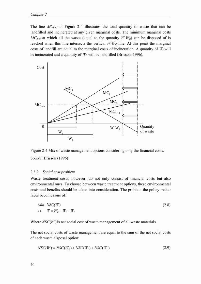
Chapter 2
40
The line MCL+I in Figure 2-4 illustrates the total quantity of waste that can be
landfilled and incinerated at any given marginal costs. The minimum marginal costs
MCmin at which all the waste (equal to the quantity W-WR) can be disposed of is
reached when this line intersects the vertical W-WR line. At this point the marginal
costs of landfill are equal to the marginal costs of incineration. A quantity of WI will
be incinerated and a quantity of WL will be landfilled (Brisson, 1996).
Quantity
of wasteW-W
R
MCL
MCL+ I
WI
WL
MCI
MCR
0
Cost
MCmin
Figure 2-4 Mix of waste management options considering only the financial costs.
Source: Brisson (1996)
2.3.2 Social cost problem
Waste treatment costs, however, do not only consist of financial costs but also
environmental ones. To choose between waste treatment options, these environmental
costs and benefits should be taken into consideration. The problem the policy maker
faces becomes one of:
)
. . R I L
Min NSC(W
s t W W W W= + +
(2.8)
Where )(WNSC is net social cost of waste management of all waste materials.
The net social costs of waste management are equal to the sum of the net social costs
of each waste disposal option:
) ( ) ( ) ( )R I L
NSC(W NSC W NSC W NSC W= + + (2.9)

Economics of waste management: key problems
41
The net social costs of each waste handling option are composed of private financial
costs (PC), external costs (EC), and external benefits of both sales of recycled
materials (Rr) or energy (Ren).
( )
( )
( )
R R R R
I I I en
L L L en
NSC W PC EC R
NSC W PC EC R
NSC W PC EC R
= + −
= + −
= + −
(2.10)
Each of the waste treatment options will lead to different costs and benefits.
Landfilling results mainly in methane emissions (in the Netherlands about 40% of the
total methane production) and incineration is a big contributor to, for example, CO2
emissions and dioxin emissions. The process of recycling is also not free from
environmental pollution (see, for example, Powell et al., 1996 and Butler and Hooper,
2000). One big disadvantage of recycling, which should also be kept in mind, is that it
is often impossible to use the material for its original purpose. Materials become
polluted when thrown away together with other waste materials. The quality of
recycled material will, therefore, be lower than the quality of virgin material. Instead
of a full recycling process, a sequence of degradation of material quality takes place.
Waste generated from high quality applications is transformed into low quality
applications (Starreveld and van Ierland, 1994). For an overview of environmental
emissions created by waste treatment in the Netherlands, see Chapter 3.
Waste treatment will also provide some benefits to society. In the case of recycling, it
is possible to sell part of the materials recovered; in the case of incineration and
landfilling, it is possible to sell recovered energy. Recovery of materials and energy
will have both financial benefits and environmental benefits in the form of avoided
financial and environmental costs caused by the production of virgin materials and
energy. In the case of paper recycling, Nakamura (1999) reveals that these benefits
may be extensive.
The optimization problem, as presented in equations 2.8 to 2.10, is illustrated
graphically in Figure 2-5. In contrast to Figure 2-4 the net social costs of the three
waste handling options, as represent in the total marginal cost line, include
environmental costs. Furthermore, recycling is no longer exogenously given to the
optimization problem, but included as an option. Akin to the previous picture, the line
MCR+L+I represents the total quantity of waste that can be disposed of, i.e. recycled,
landfilled, or incinerated, given the marginal costs. The minimal marginal cost of
disposal (MCmin) can again be determined (intersection of the W-line with the MCR+L+I
line) and the optimal quantities of recycling, incineration and landfilling can be found
(Brisson, 1996).
As shown in Figure 2-5 it is not optimal to recycle all waste. This is far too expensive,
even when the environmental costs caused by waste treatment are considered. The

Chapter 2
42
same holds for incineration as compared to landfilling. The choice between waste
handling options is also not as black and white as the waste hierarchy suggests, timing
may be of utmost importance if the government wants to minimize the costs of waste
treatment. Ready and Ready (1995), for example, illustrate that landfilling becomes
increasingly more expensive when space in the landfill is depleted. They argue that it
may be optimal if waste recycling, composting, and incineration programs are delayed
until the landfill is partially full. Highfill and McAsey (2001) find that both the wealth
of the municipality and the landfill capacity available to the municipality are
important factors in the success of recycling programs. Wealthy municipalities should
recycle as much as possible; poorer municipalities, however, should optimally rely
less on recycling and first exhaust the available landfill space.
0
Cost
MCmin
Quantity
of waste
MCL
MCR+L+I
WL
MCI
MCR
WI
WR
Figure 2-5 The optimal level of recycling, incineration, and landfilling under full
social costs
Source: Brisson, 1996
By applying a strict regime as the waste hierarchy, the government could be
stimulating inefficiently high levels of recycling and incineration, thus making society
pay far too much for waste treatment. As it is extremely hard to determine the total
social costs of waste treatment, it will be very difficult for the government to either
determine how much waste should optimally be recycled, incinerated and landfilled or
to internalize the social costs of waste treatment in the price of waste treatment.
Moreover, most countries are just starting to stimulate recycling and incineration and
to discourage landfilling. Thus, the waste hierarchy, although not optimal, may indeed
help us to channel waste management policies in the right direction as long as we bear
in mind that it is not an optimal policy tool and should not be applied mindlessly.
Economics of waste management: key problems
43
2.3.3 Estimating environmental costs
As mentioned above, it is important to determine the full social costs of waste
treatment in order to design the optimal policy mix. One of the greatest difficulties in
finding these social costs is the estimation of the environmental costs associated with
waste disposal. This requires an assessment of the amount of actual pollution that
occurs. Economic valuation or lifecycle analysis for waste disposal, for example,
could be helpful in this regard.
Economic valuation
Environmental externalities may be valued by a cost-benefit analysis (CBA). The key
principle, which underpins CBA, is very simple. The impact of the project on each
affected person is identified at each point in time. The value of any gain or loss to
each person is then estimated. These valuations should be based on the preferences of
the affected individuals, and should ideally reflect each person’s willingness to pay
for an improvement or willingness to be compensated for a loss (Perman et al, 1996).
It enables direct translation of emissions and environmental effects into costs.
One way of determining the environmental externalities of a landfill site is by using
the hedonic pricing method. For example, the development of a landfill site may
cause a temporary or permanent drop in real-estate prices in the neighboring area.
This negative value could be taken as an indicator of the costs of visual, odor, and
health effects of the landfill site (see for example Hite et al., 2001). Another useful
cost-benefit analysis is contingent valuation method (see also Hanley and Spash,
1993).
Lifecycle assessment
Life cycle assessment (LCA) is a tool to predict the overall environmental impact of a
product or service. It is defined by the society of environmental toxicology and
chemistry (SETAC) as:
“A process to evaluate the environmental burdens associated with a product, process
or activity by identifying and quantifying energy and materials used and wastes
released to the environment; and to identify and evaluate opportunities to affect
environmental improvements. The assessment includes the entire life cycle of the
product, process or activity, encompassing extracting and processing raw materials;
manufacturing, transportation and distribution; use, re-use, maintenance; recycling
and final disposal.”
SETAC (1993) p.5
For each stage, the inputs (in terms of raw materials and energy) and outputs (in terms
of emissions to air and water and as waste) are calculated, and these are aggregated

Chapter 2
44
over the total lifecycle. These in- and outputs are converted into their environmental
impacts. The overall environmental effects of the lifecycle are then calculated by
taking the sum of the environmental impacts. A comparison can thus be made
between different products or services based on their environmental impacts. Rules
for the first two stages of a LCA, namely defining the life cycle of a product and
producing an inventory of the total in- and outputs of the system have been made and
are widely accepted. Unfortunately, no rules have yet been established for the third
(impact assessment) and fourth stages (evaluation). There is still much discussion on
the one ‘correct’ way of assessing impacts and valuing these (Kirkpatrick, 1995).
In particular, the final step in a lifecycle assessment is surrounded by much
controversy. The final step in the LCA is the valuation of the environmental effects.
Comparing one lifecycle option with another will not normally show one option,
which is ‘environmentally superior’, but will demonstrate the trade-offs between the
two options. To simplify the decision-making process, attempts have been made to
aggregate the results, ultimately to a single environmental score. This involves some
weighting of the importance of different environmental problems. Not surprisingly, at
the moment there are no generally accepted objectives to weight environmental
problems. As a result, attempts so far have relied on (1) scoring systems from ‘expert
panels’, which are subjective (e.g. Landbank, 1991); (2) comparing emissions against
government targets, which are political and not global; or (3) by converting all impact
into monetary units. None of these schemes have been widely accepted. It must be
borne in mind that weighting environmental problems and aggregating them into a
single score may simplify policy choices, but by weighting them these policies
choices have implicitly already been made. Thus, broad acceptance of the outcome of
the decision is uncertain (White et al., 1997).
In most LCA studies for waste treatment, source reduction is excluded from the
model. If one is interested in minimisation of waste, it is better to use a regular LCA
instead of the more detailed LCA of waste or it is possible to use material-product
chains (see Kandelaars, 1998). Interesting LCA studies for waste treatment can be
found in CE (1996), Powell et al. (1996), White et al. (1997), and McDougall and
White (1998) .
2.4 Location problem of waste handling facilities
One aspect of the waste-handling problem has still not yet been properly addressed.
As mentioned earlier, waste management becomes increasingly difficult due to a
shortage of acceptable landfill and incineration sites. It is, therefore, important to give
due consideration to determining where the waste should be treated.

Economics of waste management: key problems
45
A couple of decades ago, waste handling was mostly a local affair. Municipalities
owned their own landfill sites and dumped the waste they collected at these sites. As
transport of waste was too expensive or impossible, there was no choice about where
waste would be treated. This situation has, however, changed significantly in the last
few decades. In the Netherlands, we see that waste management has frequently
become an issue of provincial or even national or international concern (see van
Beukering, 2001). In line with the waste hierarchy, incineration has been stimulated
instead of landfilling. Since incineration is typically one of the waste treatment
options that are too expensive on a small scale, we see that waste is transported over
longer distances. A province only has a couple of waste incineration plants, which
handle almost all the municipal solid waste generated in that province.
Until the year 2000, laws in the Netherlands forbade the transportation of waste across
province boundaries. In 2000, however, these laws were abolished. Since January
2000, municipalities and companies have been allowed to transport waste outside the
boundaries of their province and they can offer their waste to any waste treatment
unit. This means that more competition has been introduced into the waste market.
Internationally, the boundaries for waste transport are also disappearing. The laws of
the European Union already permit the export of recyclable waste. It is expected that
in a couple of years the boundaries for combustible waste will also open between the
different countries in the European Union. These facts give cause to investigate
whether the current locations of waste treatment units are optimally situated
throughout the Netherlands and the European Union.
Already there are signs that the waste market is rapidly changing. In the Netherlands
and throughout the rest of Europe, a trend towards an increasing scale, concentration,
and vertical integration as well as a merging towards a multi-utility structure, can be
identified. The waste market has become far more privatized. Energy companies have
become interested in merging with waste treatment units thus creating multi-utility
companies. Waste treatment companies are interested in vertical integration; several
of the largest companies are now focusing on providing all services connected to
waste treatment, from collection to final disposal. International companies have also
become interested in providing their services throughout the whole of Europe (WMC,
2002).
The spatial aspects of the waste treatment problem have been analyzed mostly in an
optimization setting. These studies focused on finding the optimal location of a waste
treatment center given that the waste treatment costs for society are minimized.
Examples of these kinds of studies can be found in Opaluch et al. (1993), Macauley et
al. (2002), and Ye and Yezer (1997). In Section 2.4.1, I will discuss how the waste
treatment location problem can be analyzed in an optimization model. Furthermore, in
Section 2.4.2, I will explore how it can also be analyzed within a spatial general
equilibrium framework.

Chapter 2
46
2.4.1 The spatial waste management problem: an optimization approach
There are many potential sites suitable to build a waste disposal facility. Each possible
disposal location can accommodate different annual quantities of waste and due to
economies of scale the larger the size of a landfill or incinerator, the lower the average
annual disposal costs per tonne of waste. If no transport costs are included, the
obvious least cost solution is one mammoth site handling the waste from all
municipalities. The existence of transport costs, however, complicates the issue.
Beyond a certain distance, the transport costs may well offset the benefits due to
economies of scale, making it more efficient to build additional waste handling
facilities to save on the transport costs. This problem is illustrated in Figure 2-6.
Region A
Consumer
Producer
Waste handling facility
Waste-flow
Figure 2-6 Schematic representation of location problem of waste treatment facilities.
Choosing a site is not only an economic problem that encompasses a trade-off
between transport costs and economies of scale. Rather, selecting a site involves
significant social trade-offs. For example, one technically suitable site may contain
relatively large amounts of woodland; another potential site may contain more
wetlands or farmlands. Choosing between sites implies a social preference for one
type of land over another. Similarly, one technically suitable location may be situated
near to a large residential area, while another site may have schools nearby or may
require higher costs for site development. Thus, the optimal choice includes political,
economic, and social considerations (Opaluch et al., 1993).
The optimal location may also depend on the demand for that service. For example,
Highfill et al. (1994) show that when a recycling program starts, the optimal location
of a recycling center is near the landfill site. If the recycling program becomes a
success, the optimal location will shift from the landfill site to a central location
within the municipality.

Economics of waste management: key problems
47
In addition to the financial costs of waste disposal there are potential regional impacts
on public good resources and local environmental costs that should also be taken into
consideration. At a regional level, waste treatment facilities may produce negative
effects on watersheds, aquifers, woodlands, and wetlands. Local negative impacts
include traffic congestion, odor, noise, air pollution, and the community health risks
posed by a disposal site.
To analyze the location problem of waste, a regional waste disposal model that
minimizes social costs, subject to technological, health and safety regulations can be
built. The social costs include both financial costs of waste treatment and the
monetary equivalent of the environmental costs.
Symbolically the problem can be expressed as follows (Opaluch et al., 1993):
( ) ( ),
. . ( ) 0
jMin FC J EC J where J
s t HS J
ϕ+ ∈
≥
(2.11)
Where J represent a vector of characteristics describing a site; FC(J) are the present
values of financial costs of building and operating (including transport costs) a waste
handling facility; EC(J) represents the monetary value of environmental damages; ϕ
represents a set of all possible sites and HS(J) represents technological, health and
safety constraints.
Mixed integer programming
The location problem of a waste handling facility involves a choice between different
sites. Since there are only two choices, either a waste handling facility is built on a
site or not, the problem can best be solved by a mixed integer programming (MIP)
approach. The MIP approach involves a solution of a constrained optimization
problem (cost minimization or profit maximizations) where the objective function is
linear in the activity level (variables) and where some variables can only have integer
values2.
In Malarin and Vaughan (1997), a simple mixed integer-programming model for the
waste problem is introduced. The objective is to minimize the present value of the
2 The most common areas of application are the ‘yes-or-no’ decisions. With just two choices, we can
represent such decisions by binary variables. Thus the jth yes-or-no decision would be represented by:
=no is jdecision if 0,
yes is jdecision if ,1x j
(Hillier and Lieberman, 1989)
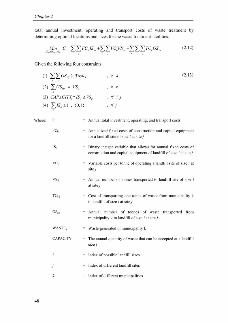
Chapter 2
48
total annual investment, operating and transport costs of waste treatment by
determining optimal locations and sizes for the waste treatment facilities:
, ,
ij kjt ij
ij js ij js ij jsIS GS VS
i j i j i k j
Min C FC IS VC VS TC GS= + +∑∑ ∑∑ ∑∑∑ (2.12)
Given the following four constraints:
(1) ,
(2) ,
(3) * ,
(4) 1 , {0,1} ,
kij k
i j
kij ij
k
i ij ij
ij
i
GS Waste k
GS VS k
CAPACITY IS VS i, j
IS j
≥ ∀
= ∀
≥ ∀
≤ ∀
∑∑
∑
∑
(2.13)
Where: C = Annual total investment, operating, and transport costs.
FCij = Annualized fixed costs of construction and capital equipment
for a landfill site of size i at site j
ISij = Binary integer variable that allows for annual fixed costs of
construction and capital equipment of landfill of size i at site j
VCij = Variable costs per tonne of operating a landfill site of size i at
site j
VSij = Annual number of tonnes transported to landfill site of size i
at site j
TCkij = Cost of transporting one tonne of waste from municipality k
to landfill of size i at site j
GSkij = Annual number of tonnes of waste transported from
municipality k to landfill of size i at site j
WASTEk = Waste generated in municipality k
CAPACITYi = The annual quantity of waste that can be accepted at a landfill
size i
i = Index of possible landfill sizes
j = Index of different landfill sites
k = Index of different municipalities

Economics of waste management: key problems
49
The first constraint basically states that the total quantity of waste treated in the waste
treatment units is equal to the total quantity of waste generated. This means that all
waste has to be disposed of and no waste can be disposed of outside the waste
treatment unit, i.e. no illegal dumping. The second constraint specifies that the total
quantity of waste sent by the municipalities to the disposal units has to be equal to the
total quantity of waste received by the disposal units. The third constraint specifies
that the total quantity of waste to be disposed of in the waste treatment facility cannot
be larger than the total capacity of the waste treatment facility. Finally, the fourth
constraint allows for only one size of waste treatment facility to be built at any one
site.
One should note that although the model is linear, the economies of scale in waste
treatment are not. Oorthuys (1995) demonstrates that although treatment costs per
tonne of waste decline when more waste is treated, no linear relationship exists
between treatment costs and size of the waste treatment unit. The economies of scale
are far larger between a small and a medium sized waste treatment unit, than between
a medium and a large sized waste treatment unit. Therefore, it is not likely that the
model will select one mammoth site waste treatment unit as the optimal solution
given that the transport costs do increase if a mammoth size waste treatment unit is
selected.
An overview of other more complex optimization models to determine the optimal
location of a waste treatment unit is presented in Fiorucci et al. (2003). A spatial
optimization model concentrating more on the economies of scale in the collection
sector can be found in Callan and Thomas (2001). They show that substantial costs
savings, of about 5%, can be made if the collection of recyclable waste and rest waste
is combined.
2.4.2 The spatial waste management problem: a general equilibrium approach
The MIP model as presented in the previous section has some major drawbacks. For
instance, it takes the quantity of waste that has to be treated as an exogenous variable.
This means that the model does not consider the interactions between waste
generation and waste treatment. The optimal treatment of a small quantity of waste
may be very different from the optimal treatment of a larger quantity of waste.
Furthermore, the treatment of waste can affect the quantity of waste that is generated.
If, for example, waste treatment becomes more expensive, households and industries
can decide to generate less waste. As less waste is generated, it may be that the
optimal location choice of waste treatment units will be affected. It is, therefore,
important to include the production, consumption, and waste treatment sectors in the
model. This can be done by using a general equilibrium model with spatial aspects
such as transport costs and economies of scale.

Chapter 2
50
To my knowledge, no research has been done to examine the interactions between
consumption and waste generation on the one hand, and waste treatment, transport
costs, and economies of scale, on the other. Building a general equilibrium model
with spatial aspects, like transport costs and economies of scale, however, has been
researched extensively. This technique has mostly been used in international trade
models. An excellent discussion on how to build various forms of spatial equilibrium
models can be found in Ginsburgh and Keyzer (1997). In Chapter 6 a spatial general
equilibrium model for the waste sector is presented and I will illustrate how spatial
aspects of the waste management problem can affect the optimal results and, more
specifically, how the quality of waste affects the optimal waste treatment method.
2.5 Conclusions
Waste generation has become a serious problem to our society. Current policies are
ineffective in dealing with this issue. The regular pricing-mechanism, a flat fee, is not
efficient and stimulates too much waste generation. Policy makers have several policy
instruments to their disposal to stimulate waste reduction. These policy tools include a
tax on waste generation, a recycling subsidy, a virgin material subsidy, an advanced
disposal fee, and a deposit refund system. All of these policy instruments have been
extensively researched. Almost all studies have concluded that a unit-based price on
the generation of waste would result in the greatest reduction of the municipal solid
waste stream. If illegal disposal, however, is an option, it is possible that consumers
will start to illegally dispose of their waste, thus rendering the use of a unit-based
price undesirable. In such a case, most studies favor the use of a deposit-refund
system; possibly combined with a small unit-based price, since of all the policy
instruments available only the unit-based price can effectively stimulate waste
prevention and home composting.
Empirical studies have demonstrated that the use of a policy instrument may be
efficient in one municipality, but not in another. The success of the policy largely
depends on the attitudes of the inhabitants of the municipality, the relative ease of
illegal disposal and the availability of recycling and re-use options. Therefore, it will
be almost impossible to design an efficient waste management plan for a larger region
or country. It will probably be necessary to design waste management plans for
individual municipalities based on the characteristics of each municipality, in the
context of a regional or national waste management plan.
In the current waste market it not possible or cost-efficient to reduce waste generation
by one hundred percent. It is, therefore, important to decide how the waste that is
generated may be treated in the least costly way, in terms of both financial as
environmental costs. The waste hierarchy provides some good indications of how we
should deal with waste. The waste hierarchy, however, should not be viewed as fixed

Economics of waste management: key problems
51
and one should exercise a degree of caution before drawing conclusions as to the
preferred waste handling option.
The location of the disposal unit also deserves some attention. It is becoming
increasingly difficult to find acceptable landfill and incineration sites. Choosing a site
involves a variety of economic, social and political considerations. The problem can
be analyzed by mixed integer programming. Mixed integer programming, however,
does not take the interaction between waste generation and waste treatment into
account. It is, therefore, of utmost importance that this problem be studied in a general
equilibrium setting.

Chapter 2
52

53
3 Waste flows and management in the Netherlands: data
and policies
3.1 Introduction
Since most of the budget for environmental problems is spent on waste management,
waste disposal can be viewed as one of the greatest environmental problems in the
Netherlands. For example, each year the Dutch government spends about 11 billion
Euros on dealing with various environmental issues. As is shown in Figure 3-1, about
38% of these costs are devoted to waste disposal. Waste disposal costs consist of the
costs of: (1) collection of waste, (2) treatment of waste and wastewater, and (3)
development and application of a large range of emission reducing technologies. In
view of these costs, it may come as no surprise that the government wishes to reduce
waste generation as much as possible.
0
2
4
6
8
10
12
1985 1990 1995 1998 1999
Expen
dit
ure
(bil
lion e
uro
s) .
Other
Climate change
Disturbance
Eutrophication
Research and development
Soil pollution
Implementation and
enforcementAcidification
Dispersion
Disposal
Figure 3-1 Environmental expenditures per theme
Source: RIVM (2001)
Since the 1990s, Dutch policy makers have attempted to stimulate the prevention and
recycling of waste. They introduced laws to force municipalities to collect rest waste
and organic waste separately. They also invested in recycling stimulation programs
and passed regulations to prevent the landfilling of combustible waste. They also
introduced a landfilling tax, which effectively raised the price of landfilling slightly
above that of incineration. Due to these measures, the quantity of waste generated by

Chapter 3
54
industry declined sharply. For example, in the construction and demolition sector, the
recycling rate went up to 94%. Households were less affected by these national
policies. On average, industry recycles about 90% of its waste; households only
recycle around 40%. The government still has a difficult task ahead of them to reduce
the quantity of municipal solid waste generated in the Netherlands.
There are several options available to deal with waste, i.e. re-use, recycling,
incineration, composting, and landfilling. Waste that is generated will either be
collected separately or will be separated after collection. If possible, any useful
materials, such as paper, metal and glass will be gathered and re-used or recycled. The
remaining waste must be treated in the most efficient way. Organic waste may be
composted; rest waste has to be incinerated or landfilled. In most discussions about
waste treatment, recycling and re-use are not considered as waste treatment options,
since these processes deal primarily with separating valuable materials from waste
and reducing waste streams. Composting, incineration and landfilling on the other
hand involve the disposal of these waste streams. In this chapter, the same distinction
between waste handling options is adopted. Thus, when a reference is made to waste
treatment, this will only refer to composting, incineration, and landfilling.
To compost or recycle waste, it is necessary to first sort the waste, preferably at the
source. Since sorting at the source depends on the goodwill of the consumer who
generates the waste, the option of mechanical separation after collection is attractive.
This would solve the problem of uncooperative households. At the VAGRON facility,
in Groningen, a new waste treatment method consisting of mechanical separation,
anaerobic digestion and incineration of municipal solid waste is tested. This facility
demonstrates that it is possible to recover about 40 to 50% of the incoming municipal
solid waste for material recycling or re-use of secondary fuel. This reduces the
quantity of municipal solid waste that has to be incinerated by 55%. This technique,
however, is still quite expensive and in an experimental phase. Therefore, in the
remainder of this thesis, the option of mechanical separation, anaerobic digestion and
incineration will be excluded from the analysis. For additional information on this
innovative waste treatment option see, for example, Oorthuys and Brinkmann (2000)
and Oorthuys et al. (2002).
This chapter provides insight into the nature of waste flows in the Netherlands and the
costs of waste treatment. To this end, a general overview of waste flows and waste
treatment options is presented in Section 3.2 and Section 3.3 provides an overview of
waste management policies. In Section 3.4, detailed information is given about the
three waste treatment options: composting, incineration and landfilling. Finally
Section 3.5 concludes.

Waste flows and management in the Netherlands
55
3.2 A general overview of waste flows in the Netherlands
Waste generation in the Netherlands has risen sharply throughout the last couple of
decades. The generation of waste tripled in the period 1960 to 1999. The growth rate
of waste generation is quite similar to the growth rate of the national economy as is
shown in Figure 3-2. Since the 1990s, the Dutch government has tried to change the
relation between the two growth rates. As stipulated in the third national environment
management plan (VROM, 1998a), the growth rate of waste generation should be
20% lower than the growth rate of the national income by the year 2010. Thus,
although, waste generation will increase in the period until 2010, it should increase
more slowly than the growth of the national income. In the first half of the nineties,
policies seemed to be very effective, as waste generation appeared to stabilize. In the
period 1994-1999, however, waste generation began to once again increase by about
2% per year (the average growth rate of the national income in this period was 3.8%
per year). The total quantity of waste generated was roughly equal to 56.6 Mtonnes
per year. As Chapter 2 illustrated, although the government succeeded in decoupling
the generation of industrial waste and economic growth, it failed to achieve a
decoupling between generation of municipal solid waste and economic growth.
0
20
40
60
80
100
120
140
160
1910 1930 1950 1970 1990
Index
1980=100
National
income
Waste
Figure 3-2 National income and waste production in the Netherlands, 1910-1999
(Index 1980=100)
Source: Adapted from VROM (1998b)
According to the Waste Management Council, the total waste stream can be divided
into 6 categories, namely: (1) municipal solid waste, which is collected from
households; (2) residues after sorting of municipal solid waste; (3) industrial waste;
(4) construction and demolition waste; (5) contaminated soil and (6) a group of other
types of waste. In Table 3-1, the quantity of waste generated per category is shown.
Municipal solid waste forms the largest category, about 40%. The quantity of
municipal solid waste generated has remained fairly constant over the last couple of

Chapter 3
56
years. Strikingly, the quantity of construction waste generated has more than halved in
the past five years; the recycling percentage for this sector has increased sharply to
94%.
Table 3-1 Categories of waste treated in Mtonnes
Category 1998 1999 2000 2001 2002
Municipal solid waste 4.9 (37%) 5.1 (37%) 5.1 (40%) 5.1 (40%) 5.0 (43%)
Residual 1.4 (11%) 1.2 (8%) 1.3 (10%) 1.4 (11%) 1.0 (9%)
Industrial waste 2.0 (15%) 2.3 (17%) 2.0 (16%) 1.9 (15%) 2.3 (20%)
Construction waste 1.2 (11%) 1.4 (10%) 1.0 (8%) 0.8 (6%) 0.5 (4%)
Contaminated soil 1.3 (10%) 1.3 (9%) 0.9 (7%) 0.5 (4%) 0.9 (8%)
Other 2.4 (18%) 2.5 (18%) 2.6 (20%) 3.0 (24%) 2.0 (17%)
Total 13.2 (100%) 13.8 (100%) 12.9 (100%) 12.7 (100%) 11.7 (100%)
Sources: WMC (2000b, 2003d)
3.2.1 The composition of the municipal solid waste stream
As shown in the previous section, municipal solid waste represents the largest
category of waste generated in the Netherlands. Municipal solid waste is also quite
diverse in nature. The municipal solid waste stream consists of several different waste
materials as can be seen in Table 3-21.
Table 3-2 Collection of municipal solid waste (in Ktonnes)
2000 2001 2002
Waste separately collected 4159 4146 4174
Organic waste 1457 1405 1416
Paper 1022 1015 993
Glass 326 335 340
Textiles 52 53 56
Small chemical waste 21 21 20
White and brown goods 43 53 59
Coarse garden waste 359 355 387
Furniture 10 14 23
Metals 76 77 70
Waste wood 225 246 262
Debris 451 437 399
Clean soil 76 90 106
Rest 41 45 43
Rest waste collected 4827 4859 4894
Total waste collected 8986 9005 9068
Source: WMC (2003a)
1 Due to differences in categories, it is difficult to compare quantities presented in Table 3.1 and Table
3.2. Table 3.1 only presents the quantities of waste composted, incinerated, and landfilled. Table 3.2
presents both recyclable waste and waste to be composted, incinerated, and landfilled.
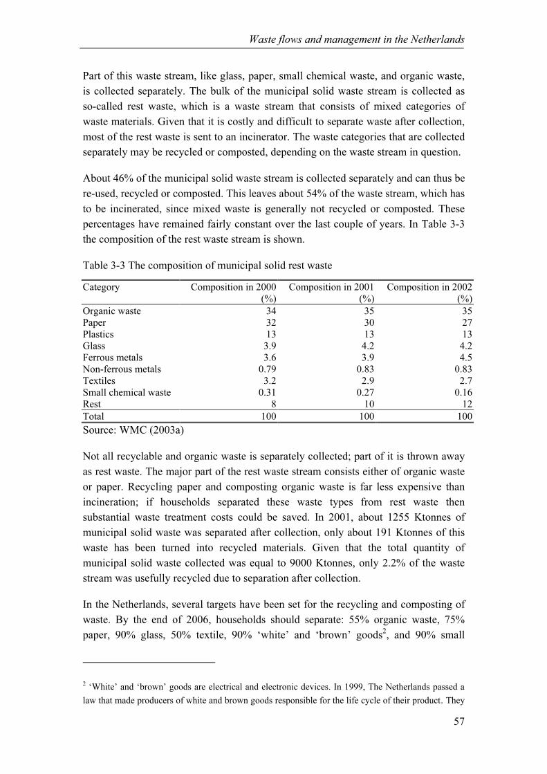
Waste flows and management in the Netherlands
57
Part of this waste stream, like glass, paper, small chemical waste, and organic waste,
is collected separately. The bulk of the municipal solid waste stream is collected as
so-called rest waste, which is a waste stream that consists of mixed categories of
waste materials. Given that it is costly and difficult to separate waste after collection,
most of the rest waste is sent to an incinerator. The waste categories that are collected
separately may be recycled or composted, depending on the waste stream in question.
About 46% of the municipal solid waste stream is collected separately and can thus be
re-used, recycled or composted. This leaves about 54% of the waste stream, which has
to be incinerated, since mixed waste is generally not recycled or composted. These
percentages have remained fairly constant over the last couple of years. In Table 3-3
the composition of the rest waste stream is shown.
Table 3-3 The composition of municipal solid rest waste
Category Composition in 2000
(%)
Composition in 2001
(%)
Composition in 2002
(%)
Organic waste 34 35 35
Paper 32 30 27
Plastics 13 13 13
Glass 3.9 4.2 4.2
Ferrous metals 3.6 3.9 4.5
Non-ferrous metals 0.79 0.83 0.83
Textiles 3.2 2.9 2.7
Small chemical waste 0.31 0.27 0.16
Rest 8 10 12
Total 100 100 100
Source: WMC (2003a)
Not all recyclable and organic waste is separately collected; part of it is thrown away
as rest waste. The major part of the rest waste stream consists either of organic waste
or paper. Recycling paper and composting organic waste is far less expensive than
incineration; if households separated these waste types from rest waste then
substantial waste treatment costs could be saved. In 2001, about 1255 Ktonnes of
municipal solid waste was separated after collection, only about 191 Ktonnes of this
waste has been turned into recycled materials. Given that the total quantity of
municipal solid waste collected was equal to 9000 Ktonnes, only 2.2% of the waste
stream was usefully recycled due to separation after collection.
In the Netherlands, several targets have been set for the recycling and composting of
waste. By the end of 2006, households should separate: 55% organic waste, 75%
paper, 90% glass, 50% textile, 90% ‘white’ and ‘brown’ goods2, and 90% small
2 ‘White’ and ‘brown’ goods are electrical and electronic devices. In 1999, The Netherlands passed a
law that made producers of white and brown goods responsible for the life cycle of their product. They

Chapter 3
58
chemical waste. These recycling and separation percentages differ a lot between
various types of municipalities. Especially in the larger cities, households are less
willing to separate waste and therefore the government has set less extensive goals in
these municipalities. None of the large municipalities, however, have achieved results
that are even close to these targets. Only the smaller municipalities are expected to
reach their targets by the end of 2006 (WMC, 2003c).
3.3 Waste management policies
3.3.1 Waste management policies throughout the years
In the beginning of the 1960s, the Dutch government became concerned about
environmental pollution. To control this pollution, legislation was introduced for each
environmental problem, the so-called sector regulation. For the waste management
problem, this led to the Hazardous Waste Law in 1976 and the Waste Material Law in
1977. Both of these laws attempted to regulate the treatment of waste.
Until the 1990s, waste management policies were mostly developed on a local and
regional scale. Provinces had some coordinating tasks, but the collection and
treatment of waste lay solely in the hands of the municipalities. In 1989, the
government realized that to deal with the waste problem cost-effectively, waste
management policies should be more centrally coordinated and developed on a
provincial and national level.
In 1990, the Waste Management Council was established. This institution, which has
representatives from municipalities, provinces and the national government, aims to
develop an effective national waste management plan. In 1992, the waste
management Council developed the ‘Ten year program for waste management’,
which determined to necessary capacity for composting, incineration and landfilling
for the period 1992-2002. In 1995, a second ‘Ten year program waste management’
program was developed for the years 1995-2005, which, apart from focusing on
planning of necessary capacity, tackled the question of how the government could
stimulate the treatment of waste according to the desired method (WMC, 1995). In
2002, the Waste Management Council published the ‘National waste management
plan’, which gives guidelines on dealing with weak points in current waste
management policies, the stimulation of more recycling, and further control of the
environmental damage caused by waste treatment (WMC, 2003e).
are required to take back their products once they are discarded and have to ensure that the products are
re-used and/or recycled in an environmentally sound manner.

Waste flows and management in the Netherlands
59
In 1993, the Dutch government adopted the concept of waste hierarchy as the basis of
national waste management policies. The waste hierarchy describes a strict order of
preferences between different waste treatment options. Prevention is preferred above
re-use; re-use above recycling; recycling above incineration and incineration above
landfilling. First of all, national waste management policies aim to reduce waste flows
as much as possible by promoting prevention and re-use of waste. The government
tries to stimulate recycling and composting by forcing municipalities to collect
organic waste and rest waste separately. Secondly, national waste management
policies aim to promote incineration and composting instead of landfilling. To
accomplish this, amongst other measures, a law was introduced in 1995 forbidding the
landfilling of combustible waste. Another measure taken by the government in 2001
was the introduction of a landfill tax to make landfilling financially less attractive
than incineration.
To reduce the environmental damage caused by waste treatment, the government
passed several laws restricting the emissions of waste treatment units, for example the
‘Dumping Law Soil Protection’ and ‘Emissions to Air Incineration Law’. Moreover,
several very strict laws were implemented to regulate the quality of secondary
materials produced by waste treatment units.
Although an extensive range of national waste management laws exist, European laws
have become increasingly important in the waste sector. These laws will be discussed
in the next section.
3.3.2 European waste management law
In recent years, the waste market has become increasingly internationally orientated.
Prior to 1994, waste management was mostly a national affair. Waste could not be
exported, since this would place an unfair burden on the environment of the importing
country. Since 1994, however, European countries have been allowed to export
recyclable waste. It is expected that within a couple of years, the borders will also be
thrown open for the export of combustible waste.
Major changes can be expected in the waste market in the next couple of years, due to
both the European Energy policy and the European waste policy.
1) The European Energy policy. The European Energy policy sets ambitious
targets for increasing the use of renewable energies and especially the use of
bio-fuels. By the end of 2010, 22.1% of the entire European energy use should
come from renewable sources. In 1997, the percentage use of renewable
energy was only 13.9%. This target is apportioned between the member states.
For the Netherlands, the target is 9% by the end of 2010.
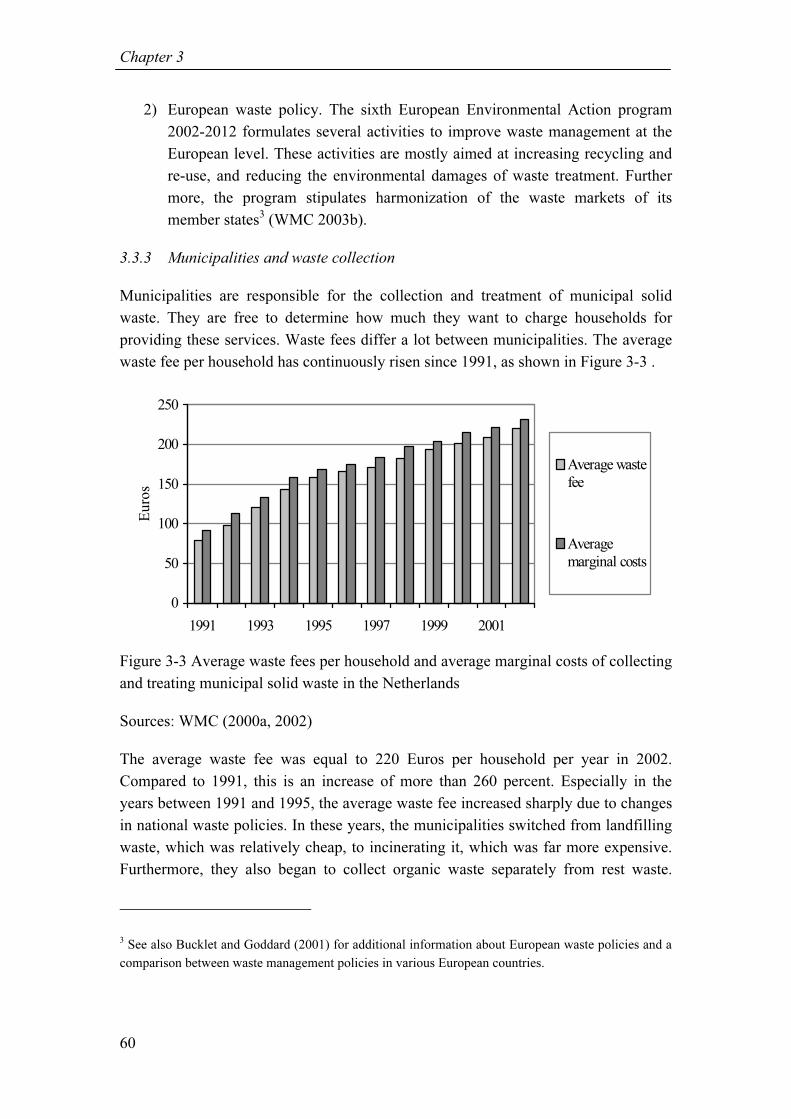
Chapter 3
60
2) European waste policy. The sixth European Environmental Action program
2002-2012 formulates several activities to improve waste management at the
European level. These activities are mostly aimed at increasing recycling and
re-use, and reducing the environmental damages of waste treatment. Further
more, the program stipulates harmonization of the waste markets of its
member states3 (WMC 2003b).
3.3.3 Municipalities and waste collection
Municipalities are responsible for the collection and treatment of municipal solid
waste. They are free to determine how much they want to charge households for
providing these services. Waste fees differ a lot between municipalities. The average
waste fee per household has continuously risen since 1991, as shown in Figure 3-3 .
0
50
100
150
200
250
1991 1993 1995 1997 1999 2001
Eu
ros
Average waste
fee
Average
marginal costs
Figure 3-3 Average waste fees per household and average marginal costs of collecting
and treating municipal solid waste in the Netherlands
Sources: WMC (2000a, 2002)
The average waste fee was equal to 220 Euros per household per year in 2002.
Compared to 1991, this is an increase of more than 260 percent. Especially in the
years between 1991 and 1995, the average waste fee increased sharply due to changes
in national waste policies. In these years, the municipalities switched from landfilling
waste, which was relatively cheap, to incinerating it, which was far more expensive.
Furthermore, they also began to collect organic waste separately from rest waste.
3 See also Bucklet and Goddard (2001) for additional information about European waste policies and a
comparison between waste management policies in various European countries.

Waste flows and management in the Netherlands
61
Since 1995, the average fee has still increased, but at a lower rate of around 5.2% per
year (WMC, 2002).
The waste fee does not cover all the costs that the municipalities make by collecting
and treating waste. The average cost coverage rate has steadily risen throughout the
last decade from about 87% in 1991 to 94% in 2002. The cost coverage rate differs
considerably between municipalities. About 70% of all municipalities have a 100%
cost coverage rate. Three municipalities, namely Eesmond, Leiden and Nijmegen
choose to charge no waste fee whatsoever so they have a cost coverage rate of zero.
Unit-based pricing
As mentioned earlier, municipalities are free to decide how much they want to charge
households for collection of waste. Many municipalities choose to make no
distinction between households based on the quantity of waste they generate. The
level of the fee is independent of the quantity of waste that is actually generated. Most
municipalities do differentiate the waste fee according to the number of persons living
in the household. Some municipalities, however, are currently experimenting with the
introduction of some sort of price differentiation based on the quantity of municipal
solid waste. In 2002, about one out of four municipalities have implemented a unit-
based pricing scheme for the collection of waste. There are several different types of
unit-based pricing schemes, i.e. according to expensive bags, volume, frequency,
weight, or a combination of these types. Table 3-4 shows the distribution of the
different types of unit-based pricing schemes over the municipalities in 2001.
Table 3-4 Distribution of different forms of unit-based pricing in 2001
System Percentage
municipalities
Percentage
households
Average number
of households per
municipality
Expensive bag 2.4 2.9 16,369
Expensive bag & size household 1.6 0.8 6,480
Expensive bag & frequency & volume 0.4 0.3 8,938
Volume 6.7 4.8 9,532
Volume & frequency 10.5 6.3 7,946
Weight 4.0 2.4 8,028
Weight & frequency 0.6 0.6 12,967
Other 1.0 0.8 11,397
Total 27.2 18.9 9,093
Size household 61 58 12,721
No differentiation 12 23 25,565
Source: WMC (2002)
Most municipalities, which have introduced unit-based pricing, favor a unit-based
price according to either volume and/or frequency. An expensive bag system, in
which households need to buy special waste disposal bags, is favored in larger

Chapter 3
62
municipalities, primarily due to the lower implementation costs. Of those
municipalities that charge a flat fee for waste collection, a majority, i.e. 61%, do
differentiate between household size. Only 12% of the municipalities apply no price
differentiation at all.
Most of the municipalities that introduced unit-based pricing are rather small. This is
understandable since unit-based pricing will be much more successful in
municipalities with a relatively low share of apartment buildings. In larger
municipalities, where the percentage of people living in apartment buildings is higher,
unit-based pricing will be less successful given that households have less space
available to compost or sort waste (Ando and Gosselin, 2003). Moreover, it will also
be more difficult and costly to implement a unit-based pricing system for households
living in apartment buildings than for households living in single-family houses. For
example, to implement unit-based pricing for single-family houses, the municipality
can choose to install weighing scales in the garbage trucks to keep track of the
quantity of waste that a household generates. In apartment buildings, waste is
normally not collected separately for each household. To introduce unit-based pricing,
the waste collection method has to be changed completely. Some municipalities have
built underground containers, which can only be accessed using a personal key, to
collect waste from households living in apartment buildings. This is, of course, far
more expensive to implement than simply modifying a garbage truck.
Table 3-5 Average fee for different unit-based pricing schemes
Average fee
(Euro/household/year)
Average waste
management costs
(Euro/household/year)
System 1999 2000 2001 2002 1999 2000 2001 2002
Volume 200 199 215 224 209 205 220 229
Volume + frequency 179 186 228 199 185 191 227 204
Expensive bag 93 109 121 126 153 155 179 180
Expensive bag & persons - - 161 177 - - 168 190
Expensive bag & volume &
frequency
- - - 203 - - - 203
Weight 169 179 194 215 188 186 200 221
Weight & frequency - - - 202 - - - 208
Rest 195 186 201 256 211 187 202 256
Average differentiated fee
depending on waste offered
170 170 186 196 190 184 199 208
Size household 188 197 207 217 198 205 221 230
No differentiation 188 200 197 206 201 210 208 219
Source: WMC (2002)
On average, the fee in municipalities that introduced unit-based pricing is 12% lower
than in municipalities without a unit based pricing scheme as shown in Table 3-5. The
percentage of cost covered, however, is also lower. Thus households pay a lower fee

Waste flows and management in the Netherlands
63
for collection of waste, while the municipalities pay more. Especially in the case of
price differentiation on the basis of expensive bags, the average fee covers only about
half the costs.
The effects of unit-based pricing
The introduction of a unit-based pricing scheme seems to reduce the quantity of
municipal solid waste generated. As shown in Table 3-6, the generation of rest waste
declines by 13% in cases of differentiation based on volume, to 59%, in case of
differentiation by expensive bags. Households begin to separate far more waste,
indeed about 10-25% more.
Table 3-6 shows that in a system with price differentiation on the basis of volume, the
total quantity of waste generated is not affected. In the other unit-based pricing
systems, the total quantity of waste generated declines. The total quantity of organic
waste generated requires some clarification. In the system with price differentiation
based on weight, households pay a variable price for the collection of rest waste as
well as organic waste. These households therefore have an incentive to reduce
generation of organic waste as much of possible. In these municipalities, the quantity
of organic waste that is home composted increases sharply. In the other unit-based
pricing systems, consumers do not pay or pay less for the collection of organic waste,
thus they have an incentive to increase their separation of organic waste from rest
waste, but they have fewer or no incentives to start home composting.
Table 3-6 Differences in waste generated per household in 1997 for different unit-
based pricing systems
System Rest
waste
Bulky
waste
Organic
waste
Paper glass
textiles
Other
separated
waste
Total
Without unit-
based pricing
0% 0% 0% 0% 0% 0%
Volume -13% -19% 28% 21% 10% 1%
Volume &
frequency
-41% -32% 1% 41% 34% -15%
Expensive bag -59% -26% 16% 36% 17% -22%
Weight -51% -29% -25% 46% 31% -23%
Source: KPMG (1999)
The figures presented in Table 3-6 suggest that unit-based pricing is quite effective in
the promotion of waste separation and recycling. However, a few words of caution are
in order. First of all, it is not exactly clear whether a straight relation between unit-
based pricing and waste separation exists. Unit-based pricing so far has only been
introduced in combination with efforts to raise the public awareness for the social
costs of waste treatment and for the benefits of recycling. Hence it is not possible to

Chapter 3
64
separate the effects of unit-based pricing and aggressive recycling programs.
Secondly, thus far unit-based pricing has only been introduced in small
municipalities, with a relatively small number of households per square mile. It is
expected that the results would be far less positive if unit-based pricing was
introduced in municipalities with a higher number of households per square mile
(KPMG, 1999).
3.4 Waste treatment options
In 2002, about 54.0 Mtonnes of waste was generated. Of this amount, about 78.5%
was re-used or recycled, which left about 11.6 Mtonnes of waste to be composted,
incinerated, or landfilled. Due to the aforementioned government regulations, the
percentage of waste landfilled has declined sharply over the last couple of years and
the percentage of waste incinerated has increased sharply. The quantity of waste
composted, incinerated, and landfilled over the last seven years are presented in
Table 3-7.
Table 3-7 Quantity of waste treated per waste treatment option in Ktonnes
Quantity of waste (in Ktonnes)
Treatment option 1996 1997 1998 1999 2000 2001 2002
Landfilling 8,450 7,400 7,100 7,600 6,550 6,530 5,157
Incineration 3,550 4,350 4,649 4,810 4,898 4,770 5,006
Composting 1,500 1,500 1,515 1,490 1,568 1,448 1,444
Total 13,500 13,250 13,264 13,900 13,016 12,748 11,607
Source: WMC (2003d)
The amounts of waste treated per category are shown in Table 3-8.
Table 3-8 Types of waste treated per waste treatment option (in Mtonnes)
Composting Incineration Landfilling
Waste category 2000 2001 2002 2000 2001 2002 2000 2001 2002
Municipal solid waste 1.5 1.4 1.4 2.7 2.8 3.0 0.9 0.8 0.6
Residual - - - 0.7 0.7 0.7 0.6 0.7 0.3
Industrial waste - - - 1.0 1.0 1.2 1.0 1.0 1.1
Construction waste - - - - - - 1.0 0.8 0.5
Contaminated soil - - - - - - 0.9 0.5 0.9
Other - - - 0.5 0.2 0.1 2.1 2.7 1.9
Total 1.5 1.4 1.4 4.9 4.7 5.0 6.5 6.5 5.3
Source: WMC (2003d)
The chosen waste treatment option varies considerably between waste categories.
Solid waste is mostly incinerated or composted; industrial waste, construction waste,

Waste flows and management in the Netherlands
65
and contaminated soil are still generally landfilled. Strikingly, almost 60% of all the
waste incinerated comes from households.
3.4.1 Composting
In the next three sections, several aspects, such as capacity, financial costs, and social
costs are discussed per waste treatment method. First of all, the various aspects of
composting will be examined.
Waste flows and composting
In 2002, a total of 1837 Ktonnes of organic waste was composted. Of this amount,
1444 Ktonnes came from households (see Table 3-8), and 152 Ktonnes from other
sources like the agricultural and forestry sector and small businesses and shops. The
remaining 241 Ktonnes derived from the separation of municipal solid waste after
collection. It is important to note that although this waste has been treated in a
composting unit, no high quality compost could be made from this waste stream. Thus
the compost coming from this source has not been sold, but instead incinerated.
In Figure 3-4, the quantity of organic waste generated by households throughout the
years is shown.
0
200
400
600
800
1000
1200
1400
1600
1800
1994 1995 1996 1997 1998 1999 2000 2001 2002
Was
te c
om
po
sted
(in
Kto
nn
es)
Figure 3-4 Quantity of municipal solid waste composted in the Netherlands in
Ktonnes
Sources: WMC (2000b, 2003d)
In 1995, the quantity of municipal solid waste composted increased significantly due
to the introduction of the Anti-dumping Law, which made it impossible to landfill
waste that could be incinerated or composted. At the same time, the government
stimulated more composting by forcing municipalities to collect organic waste and
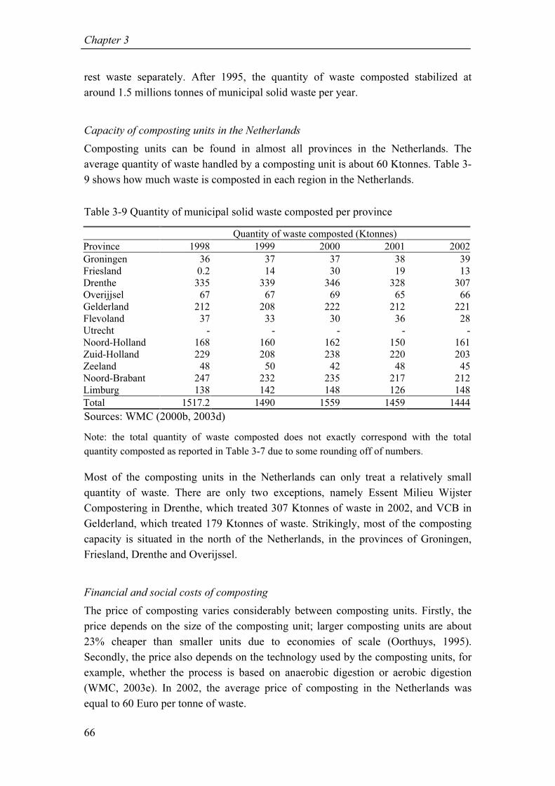
Chapter 3
66
rest waste separately. After 1995, the quantity of waste composted stabilized at
around 1.5 millions tonnes of municipal solid waste per year.
Capacity of composting units in the Netherlands
Composting units can be found in almost all provinces in the Netherlands. The
average quantity of waste handled by a composting unit is about 60 Ktonnes. Table 3-
9 shows how much waste is composted in each region in the Netherlands.
Table 3-9 Quantity of municipal solid waste composted per province
Quantity of waste composted (Ktonnes)
Province 1998 1999 2000 2001 2002
Groningen 36 37 37 38 39
Friesland 0.2 14 30 19 13
Drenthe 335 339 346 328 307
Overijjsel 67 67 69 65 66
Gelderland 212 208 222 212 221
Flevoland 37 33 30 36 28
Utrecht - - - - -
Noord-Holland 168 160 162 150 161
Zuid-Holland 229 208 238 220 203
Zeeland 48 50 42 48 45
Noord-Brabant 247 232 235 217 212
Limburg 138 142 148 126 148
Total 1517.2 1490 1559 1459 1444
Sources: WMC (2000b, 2003d)
Note: the total quantity of waste composted does not exactly correspond with the total
quantity composted as reported in Table 3-7 due to some rounding off of numbers.
Most of the composting units in the Netherlands can only treat a relatively small
quantity of waste. There are only two exceptions, namely Essent Milieu Wijster
Compostering in Drenthe, which treated 307 Ktonnes of waste in 2002, and VCB in
Gelderland, which treated 179 Ktonnes of waste. Strikingly, most of the composting
capacity is situated in the north of the Netherlands, in the provinces of Groningen,
Friesland, Drenthe and Overijssel.
Financial and social costs of composting
The price of composting varies considerably between composting units. Firstly, the
price depends on the size of the composting unit; larger composting units are about
23% cheaper than smaller units due to economies of scale (Oorthuys, 1995).
Secondly, the price also depends on the technology used by the composting units, for
example, whether the process is based on anaerobic digestion or aerobic digestion
(WMC, 2003e). In 2002, the average price of composting in the Netherlands was
equal to 60 Euro per tonne of waste.
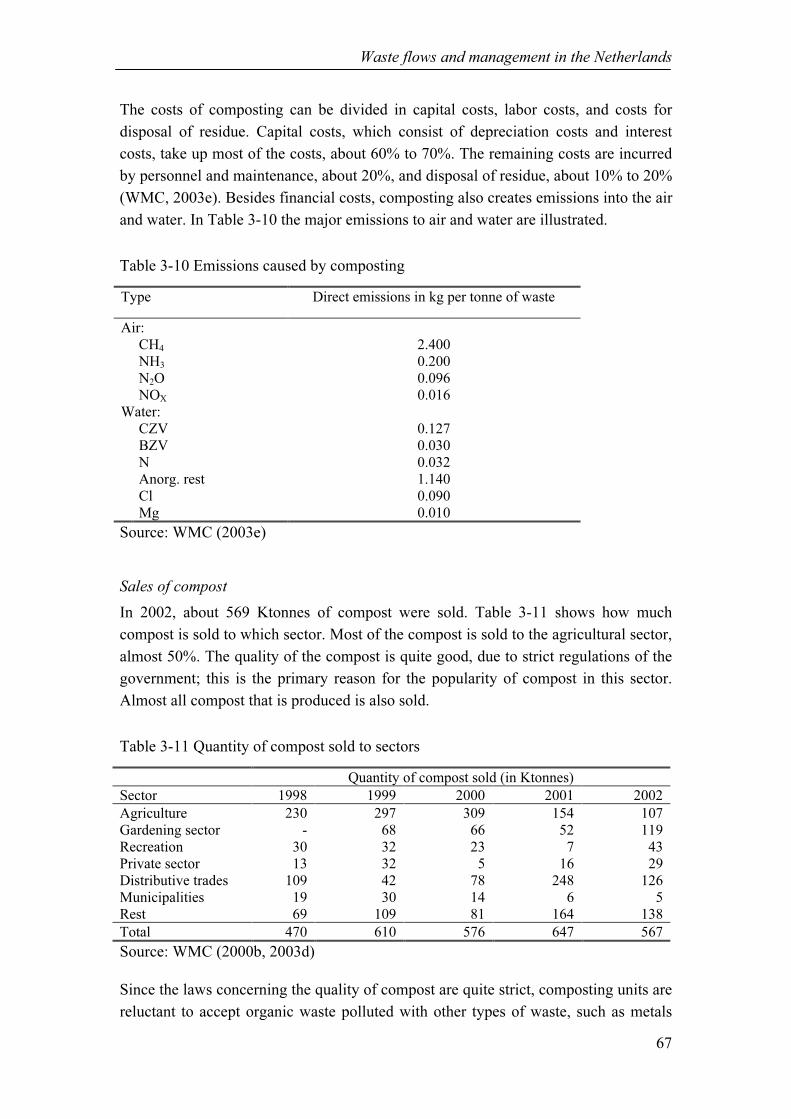
Waste flows and management in the Netherlands
67
The costs of composting can be divided in capital costs, labor costs, and costs for
disposal of residue. Capital costs, which consist of depreciation costs and interest
costs, take up most of the costs, about 60% to 70%. The remaining costs are incurred
by personnel and maintenance, about 20%, and disposal of residue, about 10% to 20%
(WMC, 2003e). Besides financial costs, composting also creates emissions into the air
and water. In Table 3-10 the major emissions to air and water are illustrated.
Table 3-10 Emissions caused by composting
Type Direct emissions in kg per tonne of waste
Air:
CH4 2.400
NH3 0.200
N2O 0.096
NOX 0.016
Water:
CZV 0.127
BZV 0.030
N 0.032
Anorg. rest 1.140
Cl 0.090
Mg 0.010
Source: WMC (2003e)
Sales of compost
In 2002, about 569 Ktonnes of compost were sold. Table 3-11 shows how much
compost is sold to which sector. Most of the compost is sold to the agricultural sector,
almost 50%. The quality of the compost is quite good, due to strict regulations of the
government; this is the primary reason for the popularity of compost in this sector.
Almost all compost that is produced is also sold.
Table 3-11 Quantity of compost sold to sectors
Quantity of compost sold (in Ktonnes)
Sector 1998 1999 2000 2001 2002
Agriculture 230 297 309 154 107
Gardening sector - 68 66 52 119
Recreation 30 32 23 7 43
Private sector 13 32 5 16 29
Distributive trades 109 42 78 248 126
Municipalities 19 30 14 6 5
Rest 69 109 81 164 138
Total 470 610 576 647 567
Source: WMC (2000b, 2003d)
Since the laws concerning the quality of compost are quite strict, composting units are
reluctant to accept organic waste polluted with other types of waste, such as metals

Chapter 3
68
and plastic. If the organic waste stream is too polluted then the composting units will
refuse to compost the waste, because even if the organic waste is cleaned and the
metals and plastics are removed it will still result in an inferior type of compost. IPH
(1995) demonstrated that on average organic waste was only 95% pure.
Unfortunately, no research has recently been conducted to determine the quality of
organic waste. Especially, when unit-based pricing is introduced, the quality of the
organic waste stream may possibly decline.
3.4.2 Incineration
The second waste treatment option discussed here is incineration. In the Netherlands,
a relatively large percentage of waste is incinerated in comparison to other western
countries. Incineration is considered to be preferable to landfilling as it first of all
does not require “eternal aftercare”, a disadvantage of landfill sites and secondly it
produces electricity and heat as a by-product. This electricity will be partly re-used in
the incineration process and partly sold to electricity providers. In some cases, the
energy produced is used to heat nearby houses or companies.
Waste flows and incineration
About 5000 Ktonnes of waste were incinerated in 2002. Since the adoption of the
waste hierarchy as basis of the national waste management policy, the quantity of
waste incinerated has steadily increased. Figure 3-5 illustrates that the quantity of
waste incinerated has nearly doubled over the last 10 years.
0
1
2
3
4
5
6
1991 1993 1995 1997 1999 2001Was
te i
nci
ner
atio
n (
in M
ton
nes
) .
Figure 3-5 Total quantity of waste incinerated each year
Sources: WMC (2000b, 2003d)
In Table 3-12, the categories of combustible waste are shown. Most of the incinerated
waste comes from households, nearly 60 percent. All rest waste collected from
households should, in theory, be incinerated. As the capacity of incinerators has not

Waste flows and management in the Netherlands
69
always been sufficient to treat all municipal solid waste, some of this waste stream
has been landfilled. The capacity of the incineration plants, however, has increased
and thus, as shown in Table 3-12, the quantity of municipal solid waste incinerated
has grown throughout the last five years. Industrial waste was mostly landfilled before
2000. Since 2000, when a landfill tax that raised the price of landfilling above the
price of incineration was introduced, the quantity of industrial waste incinerated has
increased steadily.
Table 3-12 The total quantity of incinerated waste per category (in Ktonnes)
Quantity of waste incinerated (in Ktonnes)
Waste category 1998 1999 2000 2001 2002
Solid waste 2614 2848 2710 2814 2987
Residue of solid waste and industrial waste
after central sorting 890 722 693 676 717
Industrial waste 769 891 988 977 1203
Rest 374 363 505 307 102
Total 4647 4824 4896 4774 5009
Sources: WMC (2000b, 2003d)
Note: the total quantity of waste incinerated does not exactly correspond with the total
quantity incinerated as reported in Table 3-7 due to some rounding off of numbers.
Capacity of incineration plants
There are 12 waste incineration plants in the Netherlands. Together they have a
capacity to treat about 5.5 million tonnes of waste.
GAVI
Wijster
AVI Twente
Hengelo
AVIRA
DuivenARN
Weurt
Huisvuilcentrale NH
Alkmaar
AVI-A
Amsterdam
AVR Rijnmond&AVR-R
Rotterdam
GEVUDO&ZAVIN
DordrechtAZN
Moerdijk
SITA
Roosendaal
Figure 3-6 The location of incineration plants in the Netherlands

Chapter 3
70
The location of waste incineration plants is illustrated in Figure 3-6. Most of the
capacity for waste incineration can be found in the west and the north of the
Netherlands. Landfilling was quite expensive in the north because the soil was
unsuitable for landfilling and in the west due to a shortage of available land. In the
south, both enough space was available and the soil was suitable for building landfill
sites. In the south, therefore, landfilling was considered to be the optimal waste
treatment option. Only during the last five years, following the government’s
prohibition of the landfilling of combustible waste did the south start to invest in
incineration plants.
The total quantity of waste treated in each installation is shown in Table 3-13.
Table 3-13 Total quantity of waste treated in incineration plants
Quantity of waste incinerated (in Ktonnes)
Province Installation 1998 1999 2000 2001 2002
Drenthe GAVI-Wijster 413 433 441 425 422
Overijssel AVI Twente 288 284 284 290 289
ARN 237 250 239 245 269Gelderland
AVIRA 297 287 315 336 339
Huisvuilcentrale NH 450 450 448 460 464Noord-
Holland AVI Amsterdam 790 761 801 795 827
AVR rijnmond 975 1040 1098 1086 1120
GEVUDO 194 171 215 212 207
AVR Afvalverwerking Rotterdam 385 386 391 375 383
Zuid-
Holland
ZAVIN 7 7 7 7 7
SITA Roosendaal 49 55 54 50 52Noord-
Brabant AZN 561 603 605 489 628
Total quantity of waste incinerated 4649 4810 4898 4770 5006
Sources: WMC (2000b, 2003d)
Note: the total quantity of waste incinerated does not exactly correspond with the total
quantity incinerated as reported in Table 3-7 and Table 3-12 due to some rounding off of
numbers.
Since the opening of the provincial borders for transport of waste in January 2000,
waste incineration plants are able to accept waste from all over the country. The
operational scale of the incineration plants has gone from regional to national.
Moreover, several waste incineration plants (Gavi-Wijster, ARN and AVI-Twente)
are planning to focus more on treatment of foreign waste (WMC, 1997).
Financial and social costs of incineration
The average cost price for incineration in 2002 was equal to 110 Euros per tonnes of
waste. Figure 3-7 shows the cost price for incineration plants in 2002.

Waste flows and management in the Netherlands
71
0
20
40
60
80
100
120
140
160
Wij
ster
Tw
ente
AV
IRA
AR
N
HV
C
A'd
am
AV
R
SIT
A r
oo
sen
daa
l
GE
VU
DO
AZ
N
Co
st p
rice
(E
uro
per
to
nn
e) .
Figure 3-7 The price of waste incineration in 2002 for the incineration plants (in Euro
per tonnes)
Source: WMC (2003b)
Waste incinerator ARN in Nijmegen was clearly the most expensive company, and
HVC in Amsterdam the cheapest. The price of incineration depends on the size of the
incineration plant. On average, a large incineration plant is about 41% less expensive
than a small incineration plant due to economies of scale.
The cost price of incineration is determined by a total of capital costs, operational
costs and operational benefits. Figure 3-8 illustrates the extent to which capital costs,
operational cost, and benefits varied for each installation in 1996.
-100%
-50%
0%
50%
100%
150%
200%
Gav
i-W
ijst
er
AV
I T
wen
te
AV
IRA
AR
N
HV
C
AV
I-A
'dam
AV
R
RO
TE
B
GE
VU
DO
AZ
N
operational costs
capital costs
operational benefits
Figure 3-8 Composition of cost price of incineration of waste
Source: WMC (1997)

Chapter 3
72
The greater the operational benefits, the lower the cost price will be. The capital costs
consist of depreciation costs and interest costs. The operational costs are defined as
the maintenance costs, costs of landfilling, the residues of incineration, energy costs,
cost of personnel and other operating costs. The operational benefits consist of the
sales of energy and the sales of metal and others useful residues. The large variation
of benefits between the different incinerators is particularly interesting. AVR had the
highest percentage of benefits, GEVUDO the lowest.
The incineration of waste creates emissions into the air and groundwater. In 1989,
there was great commotion about the generation of dioxins by incinerators.
Incinerators barely filtered dioxins from the smoke they emitted and this turned out to
be a serious health hazard. Toady, incinerators filter almost all dioxins from emitted
smoke; however, some other substances are still emitted. In Table 3-14, the most
important emissions to air and water are shown.
Table 3-14 Emissions caused by incineration (per tonne of waste)
Direct emissions per tonne of waste
Air (in kg)
CO2 467
CH4 0.03
SO2 0.20
NOx 0.21
Dioxins (in mg) 0.00255
Water (in mg)
Cd 5.2
Cr 4.5
Cu 5.5
Ni 2.1
Pb 1.2
Hg 0.72
Chemical waste (in kg) 21.80
Sources: WMC (2003e) and CE (1996)
Municipalities and Incinerators
In the Netherlands, municipalities and incinerators are inextricably linked. Contracts
between municipalities determine the quantity of waste municipalities to be delivered
to the incinerator and the price paid for waste treatment. Most of the waste treated in
incinerators comes from municipalities. Figure 3-9 shows the percentages of
industrial and municipal solid waste treated in incinerators in 2002. The average
percentage of solid waste treated in incinerators is equal to 74 percent. Essent Wijster
in Drenthe and ARN in Gelderland only treat solid waste from households. AZN in
Noord-Brabant treats the largest percentage of industrial waste, 47% of all waste
treated in AZN comes from industrial sources.

Waste flows and management in the Netherlands
73
0%
10%
20%
30%
40%
50%
60%
70%
80%
90%
100%
Ess
ent
Wij
ster
AV
I T
wen
te
AV
IRA
AR
N
HV
C
AV
I-A
'dam
AV
R
RO
TE
B
GE
VU
DO
AZ
N
HV
R
aver
age
industrial
waste
solid
waste
Figure 3-9 Percentage of solid and industrial waste treated in incinerators
Source: WMC (2003d)
Since almost all municipalities in the Netherlands have contracts with incinerators, the
supply of municipal solid waste is more or less guaranteed. These contracts were
introduced due to the necessity of promoting incineration. The starting cost of
building an incineration plant were quite high and the market for incineration was
rather unstable. Therefore, it was difficult to get companies interested in building an
incinerator without some form of insurance. The contracts between municipalities and
incinerators gave incinerators a right of existence. These contracts could be used as
collateral to finance the investment costs of an incinerator. Moreover, some
municipalities provided guarantees for financial obligations or possible losses. Due to
these guarantees, financing the building and operation of incineration plants became
less risky and the capital costs were reduced significantly (WMC, 1999).
However, the downside of the contracts and financial guarantees is that it is fairly
easy for the incinerators to transfer operational risks to the municipalities. Thus the
risk of operation lies partly or completely with the municipalities and therefore with
the households, who pay for waste incineration through waste fees (WMC, 1999 and
Dijkgraaf et al., 1999).
3.4.3 Landfilling
The final waste treatment method under discussion is landfilling. Landfilling
encompasses the controlled dumping of waste in specific sites and is in fact the least
preferred method of waste treatment according to the waste hierarchy, as discussed in
Chapter 2. Since landfilling does not fit into the concept of closed material cycles, the
government does not approve of landfilling and has striven to discourage it as much

Chapter 3
74
as possible. One should, however, bear in mind that is not yet possible to eliminate
landfilling completely as a means of dealing with waste. Both incineration and
composting, for example, will produce a residue, which has to be landfilled.
Moreover, the capacity of incinerators is as of yet not large enough to handle all
combustible waste, thus part of this waste will inevitably have to be landfilled.
Waste flows and landfilling
Most of the waste treated in landfill sites stems from the industrial sector and the
construction and demolition sector. The percentage of solid waste that is landfilled
has declined sharply due to policies of the government, as can be seen in Table 3-15.
Table 3-15 Quantity of waste landfilled per waste category
Quantity of waste in Ktonnes
Waste category 1998 1999 2000 2001 2002
Solid waste 800 800 950 800 592
Rest waste after sorting 500 550 600 650 329
Industrial waste 1200 1450 1000 1050 1054
Cleansing department waste 150 150 250 300 96
Shredder waste 150 100 100 150 131
Construction and demolition waste 1200 1400 1000 800 461
Contaminated soil 1250 1250 900 500 854
Non-contaminated soil 200 300 250 350 103
Purification silt 350 250 150 200 21
Rest 1300 1350 1400 1800 1516
Total 7100 7600 6600 6600 5157
Sources: WMC (2000b, 2003d)
Note: the total quantity of waste landfilled does not exactly correspond with the total quantity
landfilled as reported in Table 3-7 due to some rounding off of numbers.
The Anti-dumping Law does not permit the landfilling of combustible waste. Since
the capacity of incineration plants was insufficient, municipalities were occasionally
exempted from this regulation. In 2003, however, the government decided that the
incineration capacity was sufficient to treat all municipal solid waste and thus, as of
2003, municipalities will no longer be able to be exempted from the Anti-dumping
Law. (WMC, 2003e).
Capacity of landfill sites
As shown in Figure 3-10, the quantity of waste landfilled has declined sharply
throughout the past decade. Figure 3-10 illustrates that the quantity of waste landfilled
dropped sharply in 1995 due to the introduction of the afore mentioned Anti-dumping
Law. In 1999, the quantity of waste landfilled rose slightly. This is partly due to the
low costs of landfilling as compared to other treatment options.

Waste flows and management in the Netherlands
75
0
2
4
6
8
10
12
14
1992 1994 1996 1998 2000 2002Am
ou
nt
of
was
te l
and
fill
ed
.
(in
Mto
nn
es)
Figure 3-10 Quantity of waste landfilled in Mtonnes
Sources: WMC (2000b, 2003d)
Although in theory waste cannot be landfilled due to the Anti-dumping Law, it is still
possible to get an exemption. Industries in particular are very keen on being awarded
an exemption, since the price of landfilling is much lower than the price of
incineration. In 2000, the government introduced a substantial tax on landfilling to
raise the price of landfilling above that of incineration; thus providing industries with
an incentive to incinerate and recycle waste.
Not every province landfills the same quantity of waste. Table 3-16 shows the
quantity of waste landfilled in each province.
Table 3-16 The quantity of waste landfilled per province in the Netherlands
Quantity of waste
landfilled (Mtonnes)
Rest capacity
(Mtonnes)
New capacity
(Mtonnes)
Province 2000 2001 2002 2000 2001 2002 2000 2001 2002
Groningen 0.23 0.31 0.26 1.5 1.3 1.2 - - -
Friesland 0.29 0.26 0.31 0.5 2.1 1.9 1.2 - -
Drenthe 0.54 0.64 0.42 5.1 5.8 5.4 - - -
Overijjsel 0.49 0.34 0.35 5.4 5.2 5.3 3.7 3.7 3.7
Gelderland 1.1 1.19 1.1 8.8 8.6 8.1 4.6 4.6 4.6
Flevoland 0.09 0.09 0.15 0.5 0.6 0.4 4.2 4.2 4.2
Utrecht 0.18 0.18 0.15 1 3.3 2.7 2.6 - -
Noord-
Holland 1.01 0.99 0.78 6.2 5.3 4.9 3.7 3.7 3.7
Zuid-Holland 0.92 0.89 0.58 8.1 6.4 6 - - -
Zeeland 0.3 0.25 0.24 1 2.5 2.3 1.5 - -
Noord-
Brabant 0.94 0.99 0.54 10.8 8.6 9.4 - - 0.7
Limburg 0.46 0.4 0.27 9.5 6.8 6.6 0.4 - -
Total 6.55 6.53 5.15 58.4 56.5 54.2 21.9 16.2 16.9
Source: WMC (2003d)
Note: the total quantity of waste landfilled does not exactly correspond with the total quantity
landfilled as reported in Table 3-8 and Table 3-15 due to some rounding off of numbers.

Chapter 3
76
In 2002, there were 30 landfilling sites in use, 17 landfilling sites in the process of
being closed, 3 new sites being built, and 4 sites temporarily closed. The total
capacity per province is also given in Table 3-16. Strikingly, most of the landfill
capacity is situated in the south of the Netherlands. As explained above, landfilling
was attractive in the south due to availability of space. Only after it became evident
that the government was going to discourage landfilling, did the south start
concentrating on the incineration of waste. This is in contrast to the north of the
Netherlands, where the soil was not suitable, and the west of the Netherlands, where
space was too valuable.
Financial and social costs of landfilling
The price of landfilling has significantly increased over the last twenty years. In Table
3-17 the average prices of landfilling are provided. These average prices include the
tax on landfilling. The tax on landfilling of combustible waste constitutes about 62%
of the total costs of landfilling. The tax on landfilling of non-combustible waste is
about 13% of the total costs. As can be seen in Table 3-17, since 2000, the average
price of landfilling including the tax has been higher than the average price of
incineration.
Table 3-17 Average price of landfilling and incineration (Euro per tonne)
1985 1990 1995 1998 2000 2001 2002
Landfilling of
combustible waste
10 27 78 93 110 107 128
Landfilling of non-
combustible waste
10 27 48 63 60 56 58
Incineration 45 64 101 95 101 99 106
Source: RIVM (2003)
The operational costs of landfilling are divided as follows: about 15% of the costs are
spent on personnel and maintenance; about 10% of the costs are spent on the aftercare
tax and the remainder, about 75%, is spent on capital costs, which consist of
depreciation costs and interest costs (Statistics Netherlands, 2002a). Landfill sites
require eternal aftercare to prevent leakages to ground water at some point in the
future. In 1996, the provinces were made responsible for taking care of the eternal
aftercare for landfill sites within their borders. The provinces thus decided to tax
landfill sites. The average aftercare tax is currently about 5 Euros per tonne of waste.
Landfilling can lead to emissions into both air and groundwater. It is inevitable that
some emissions will occur, even if the best available techniques to prevent leakage are
employed. Some biogas can be won back from the waste, thus reducing the energy
costs of landfilling.

Waste flows and management in the Netherlands
77
The process of landfilling works as follows: firstly, waste will be dumped in a
landfilling site. Then it is covered up. For about 15 years the landfill site will be
exploited in the sense that gas produced in the landfill site is captured and used to
produce electricity. After 15 years, the landfill site will be closed and remaining gas
will flared. Table 3-18 shows the emissions to air and water that occur during the
landfilling process. Most of the emissions occur during the dumping process of waste;
they are known as direct emissions. During the process of electricity generation from
the landfilling gas, (called gas motor in the table) and during the process of flaring the
remaining landfill gas, some emissions to NOx will occur.
Table 3-18 Emissions and chemical waste caused by landfilling (per tonne of waste)
Emissions to air, water and production of chemical waste per
tonne waste
Emissions Direct Flaring Gas motor Total
Air (in kg)
CO2 0 0 0 0
CH4 10.44 0 0 10.44
SO2 0 0 0 0
NOx 0.015 0.01 0.23 0.255
Water (in mg)
As 4.8
0 0 4.8
Cd 0.144
0 0 0.144
Cr 9.0
0 0 9.0
Cu 2.4
0 0 2.4
Ni 6.0
0 0 6.0
Pb 2.7
0 0 2.7
Hg 0.9
0 0 0.9
Chemical waste (in kg) 2.0 0 0 2.0
Source: CE (1996)
3.5 Concluding remarks
The waste market in the Netherlands is quite well documented. The Waste
Management Council collects a lot of data each year. There have been several
significant changes in the waste market during the last 10 years. Due to governmental
regulations, far more waste is now being incinerated or composted instead of
landfilled. Recycling percentages of waste have also increased. On average, about
79% of all waste generated in the Netherlands is recycled. These high recycling
percentages are mostly due to the high recycling percentages in the industrial sectors.
The industrial sectors recycle on average about 90%. Households do not recycle
nearly as much, only about 40%.
To stimulate households to recycle more and generate less rest waste, some
municipalities have introduced unit-based pricing for waste collection. The early
results seem positive. If unit-based pricing is introduced, households tend to generate

Chapter 3
78
far less rest waste and separate far more useful materials from the rest waste stream. It
is, however, difficult to determine how significant the effect of unit-based pricing is.
Thus far unit-based pricing has always been introduced in combination with recycling
programs. Introducing unit-based pricing is also quite expensive, so the question
remains whether the initial costs of introducing the system will be compensated by the
lower costs of waste collection and treatment.
In Chapters 4, 5 and 6, the data presented here will be used to analyze different
aspects of the waste market. With the analysis presented in those chapters, I especially
hope to clarify the costs and benefits of a unit-based pricing system and determine
which municipalities should indeed introduce a unit-based pricing system.

79
Part II
Modeling waste management problems

80

81
4 Modeling market distortions in an applied general
equilibrium framework: the case of flat fee pricing in the
municipal solid waste market1
4.1 Introduction
Current waste management policies are inadequate to achieve a significant reduction
in generation of municipal solid waste. Although governments have made great
efforts to reduce waste generation, the actual quantity of waste generated has
continued to rise. This is mostly due to economic growth. As shown in Chapter 2,
governments have failed to achieve a decoupling between waste generation and
economic growth due to presence of market distortions in the municipal solid waste
market. In the Netherlands, these market distortions are (i) flat fee pricing, (ii) virgin
material biased policies, and (iii) killer-contracts between municipalities and waste
treatment facilities. All of these market distortions can lead to the market failure
whereby waste generation is higher and recycling lower than is socially optimal, thus
incurring inefficiently high waste treatment costs (Miedema, 1983).
Several studies have been conducted to analyze the effects of these market distortions
and to suggest possible solutions. Wertz (1976) found that the introduction of a user
charge for waste collection led to a significant reduction of waste generation.
Miedema (1983) showed that a virgin material tax could reduce waste generation.
Other more recent studies include Jenkins (1993), Hong et al. (1993), Miranda et al.
(1994), Morris et al. (1994) and Sterner and Bartelings (1999). The overall conclusion
of these empirical studies is that the demand for waste services is sensitive to unit-
based pricing. The introduction of a unit-based price can lead to a substantial
reduction in waste generation, especially if combined with programs that increase
public awareness of the waste problem. However, imprudent construction of unit-
based pricing may not have the desired effect and can even encourage illicit dumping,
burning or other improper disposal (e.g. Fullerton and Kinnaman, 1995).
Although most studies agree that a flat fee pricing system is not optimal, they do not
agree on optimal policy choice to minimize cost of disposal. Studies, such as
1 This chapter is adapted from: Bartelings, H., R.B. Dellink and E.C. van Ierland. Modeling market
distortions in an applied general equilibrium framework: the case of flat fee pricing in the waste
market. In: J.C.J.M. van den Bergh and M. A. Janssen (eds) Economics of industrial ecology.
Cambridge: MIT press (forthcoming).

Chapter 4
82
Miedema (1983), Jenkins (1993), Strathman et al. (1995) and Linderhof et al. (2001),
have proposed the introduction of a ‘downstream’ tax, which would increase the price
of disposal. Other studies, like Fullerton and Kinnaman (1995; 1996); Palmer and
Walls (1997); Fullerton and Wu (1998) and Choe and Frasier (1999), favor an
‘upstream’ tax, which internalizes the costs of waste treatment in the price of the
consumption good. They fear that a ‘downstream’ tax would be non-optimal due to
huge implementation and enforcement costs.
In this chapter, a general equilibrium model is developed to analyze the efficiency of a
‘downstream’ tax, namely the unit-based pricing scheme, and an ‘upstream tax’,
namely the advanced disposal fee (or waste tax). The general equilibrium approach
makes it possible to include the entire product life cycle, from extraction, production,
consumption, and collection to final disposal. Policies that attempt to reduce waste
disposal will affect all of these stages. New in the analysis is the explicit role of the
municipality as collector of waste. The method of solid waste collection, pricing of
waste collection and the subsequent choice of waste treatment options lies solely with
the municipality; the municipalities, therefore, have a significant effect on the social
costs of waste treatment.
The effects of waste policy options available to the government are also analyzed in
this chapter. To make a fair analysis between different policy options both
implementation and enforcement costs of introducing these policy options are
included in the model.
This chapter is structured as follows: Section 4.2 describes the model and provides
some insights into how different policy options can be included in an applied general
equilibrium model. Section 4.3 presents a stylized example based on numerical data
from the Netherlands collected in 1996 and shows how different waste management
policies can affect waste generation. Section 4.4 concludes and offers some policy
recommendations.
4.2 Description of the model
4.2.1 Introduction
In this section, an applied general equilibrium model of the waste market is presented
with the use of three sub-modules. Section 4.2.3 describes the sub-module, which
includes unit-based pricing for waste collection, Section 4.2.4 explains the sub-
module, which includes flat fee pricing, and Section 4.2.5 describes the sub-module,
which includes an upstream tax.
As described in Chapter 1, there are several formats that can be used to build a general
equilibrium model, for example the ‘Computable General Equilibrium format’, the

Modeling market distortions in an applied general equilibrium framework
83
‘Open economy format’, the ‘Full format’, and the ‘Negishi format’. Some of these
formats are written in terms of excess demands, other in terms of welfare programs.
Extensive information about the strengths and weaknesses of each of these formats
can be found in Ginsburgh and Keyzer (1997). However, it should be stressed that a
format is simply a way of presenting a model. A different format will still describe the
same model and result in the same equilibrium solution.
In this chapter, a general equilibrium model is built according to the Negishi format.
The advantage of this format is that it is relatively easy to incorporate externalities
and non-convexities (see also Ginsburgh and Keyzer, 1997). Hence this format is
particularly suitable for incorporating market distortions like flat fee pricing.
4.2.2 The subsidy-cum-tax scheme
Most municipalities have chosen to charge a fixed amount of money for waste
collection, the so-called flat fee. In a flat fee-pricing scheme, the amount of money
paid for waste collection is independent of the quantity of waste actually generated.
The perceived price for waste collection, in economic terms the marginal perceived
costs of generating waste, equals zero in such a case. If the price of a good equals zero
the equilibrium demand for that good can no longer be determined through the normal
demand and supply functions. In the general equilibrium framework in particular,
where it is assumed that some equilibrium price will ensure that demand equals
supply, the zero price poses a problem. To implement a zero price in a general
equilibrium model, we thus require an indirect approach. It is possible to implement a
zero perceived price by using subsidies that compensate households for the cost of
waste generation.
Households pay a fixed lump-sum transfer to the government for the collection of
waste, based on the flat fee. This lump-sum transfer takes away part of the
households’ income. Therefore, the total expenditure of the households declines. The
expenditure pattern, i.e. the percentage of income the households spend on a certain
product will, however, not be affected.
In the model presented in this chapter, private households demand waste collection
services and pay an equilibrium price for these services. To introduce the zero
perceived price, the government reimburses these costs to the consumers in the form
of a subsidy, which equals the equilibrium price for every unit of waste collection
services exactly. Thus, the perceived price of waste collection for the households
equals zero. If the revenue of the lump-sum transfer is lower than the amount spent on
the subsidy, the government expenditure decreases (in this case there is a net subsidy
on waste generation). If the revenue of the flat fee is higher than the total costs,
government expenditure increases. The idea of the subsidy-cum-lump-sum transfer
scheme is illustrated in Figure 4-1.

Chapter 4
84
Flat fee
Private
households
Consumption
good
Municipality
as collector
of waste and
as consumer
price good
price subsidy collection
services
Real money
transfer
Transfer goods
Hypothetical
money transfer
Figure 4-1 The subsidy-cum-tax scheme
Section 4.2.4 shows how the subsidy-cum-tax scheme can be implemented in a
general equilibrium model.
4.2.3 Description of the model including a unit-based price for waste collection
In a simplified economy, two types of actors are distinguished: households and firms.
Households consume goods and supply endowments; firms produce goods with the
use of endowments and intermediate goods. Consumers are differentiated into two
types: private consumers and a government consumer. Five different production
sectors are distinguished, together producing eight unique goods. These sectors are:
(1) an extraction sector producing virgin material; (2) a production sector producing
agricultural goods, industrial goods and services; (3) a recycling sector producing
recycling services; (4) a collection sector producing collection services and (5) a
waste treatment sector producing incineration services and landfilling services. The
hypothetical economy is shown in Figure 4-2.
Private households consume the consumer goods: agricultural goods, industrial goods,
and services. The government consumes only services. Consumption of agricultural
and industrial goods leads to the generation of municipal solid waste. Waste must be
either recycled or collected by the municipality. We assume that collected rest waste
is not separated and recycled after collection, but is instead sent immediately to an
incineration plant or landfill unit. Although this puts some constraints on the model,
we feel that this assumption is justified. We are primarily interested in the choice the
consumer makes: the consumer can, for example, choose to separate organic waste,
paper, or glass from rest waste. The consumers will have to incur costs in order to
recycle these materials. Recycling will, for example, cost the consumer both time and
storage space. This is modeled as if the consumer buys ‘recycling services’. By

Modeling market distortions in an applied general equilibrium framework
85
buying recycling services, they generate recyclable waste; this waste is sent to a
recycling unit where it is turned into recycled material.
(1) Extraction
(2) Production
Services
Industry
Agriculture
Virgin material
(3) Recycling
Consumption
Government
Private households
(4) Collection
(5) Waste Treatment
Incineration
Landfilling
Recycled material
Goods
Waste
Waste
Waste suitable
for recycling
Figure 4-2 Representation of the hypothetical economy
Consumers can prevent waste by recycling more or, to a lesser extent, by substituting
waste intensive goods, i.e. agricultural and industrial goods, for waste extensive
goods, i.e. services. In reality, consumers have the possibility of two kinds of
substitution, namely substitution within a sector and substitution between sectors.
Substitution within a sector makes it possible to choose between two products that are
basically the same except for waste intensity. Substituting between sectors would
mean changing consumption patterns. For example, in Oostzaan, a municipality where
a unit-based pricing scheme was recently introduced, households reported that they
not only bought more products containing less packaging, an example of substitution
within a sector, but also began to use diaper services instead of disposable diapers, an
example of substitution between sectors (Linderhof et al., 2001). Waste prevention
through substitution within a sector would add a certain degree of complexity to the
model, as different products within the same sector and their associated 'waste
intensity' would have to be explicitly modeled. In our opinion, this trade-off between
accuracy and transparency of the model is not easy to make, but in this case we have
chosen to include only the more straightforward channel of waste prevention through
substitution between sectors. As a consequence, the possibility of waste prevention –
and thus also the effects of introducing either a unit-based price of an upstream waste
tax - may, therefore, be underestimated. This assumption, however, will not affect the
comparison between the effectiveness of a unit-based price and an upstream waste
tax, since the substitution possibilities will be identical in these two scenarios.
We assume that only private households generate waste. Both the government
consumer and firms do not generate waste. we made this assumption (although not
completely realistic) because the focus is on policies affecting the generation of

Chapter 4
86
municipal solid waste, and not on policies that affect the generation of industrial or
government waste.
All the firms use capital and labor to produce goods or services. The extraction sector
produces virgin material, which is sold to the production sector of consumer goods.
The recycling sector sells recycling services to the consumer and recycled material to
the production sector of consumption goods. Besides capital and labor, the production
sector of consumption goods uses virgin materials and recycled materials as inputs to
production. The collection sector sells collection services to private households. They
use capital, labor, and waste treatment services as inputs. Finally, the waste treatment
sector sells waste treatment services to the collection sector. It consists of two
producers: a producer of incineration services and a producer of landfilling services.
Consumer utility function
In the Negishi format, total welfare is maximized subject to utility, balance, and
production possibility constraints (Ginsburgh and Keyzer, 1997). The total welfare
function is shown in equation 4.1. Total welfare (TW) equals the sum of weighted
utilities (ui) over consumer i ( i=1,...,n) .
( ) ( )gi i i i
i
TWF Max u xα α= ∑ (4.1)
Consumers derive utility from the consumption of consumer goods (xig) where g=
agricultural goods, industrial goods and services. The utility of each consumer is
weighted by a factor αi, the so-called Negishi weights.2
Consumers generate waste by consuming products. Waste generation is dynamic; not
all products will be transformed into waste immediately after consumption. Durable
goods, for example, can continue to function properly for several years. If one looks at
an infinite time scheme, every good will turn into waste. At any point in time,
however, only part of the products will be transformed into waste. To include this
dynamic aspect in a comparative static model, waste is determined as a fraction β g of
the consumption product3. Total waste generation per consumer (Wi) is equal to a
2 These Negishi weights are determined in such a way that each consumer’s budget constraint holds.
This means that consumers cannot spend more money on goods and services than they receive on sales
of primary inputs (capital and labor). The value of the Negishi-weights is exogenous to the model. How
these Negishi weights are determined and how the equilibrium solution is found is described in
appendix 4-A. See Ginsburgh and Keyzer (1997) for more information.
3 Implicitly this means that part of the used material accumulates in a stock of durable goods. This
stock is not constant, new materials enter the stock and other materials leave the stock as waste.

Modeling market distortions in an applied general equilibrium framework
87
fixed percentage of total consumption. The fraction of waste contained in a product
differs for the three types of consumption goods. Agricultural and industrial goods are
relatively waste intensive and thus β will be positive for these goods; consumption of
services does not generate waste and thus β is equal to zero in this case. The
government only consumes services and does not generate waste, therefore, in the
following equation a subset c is used, which encompasses only the private
households.
g g
c c
g
W xβ=∑ (4.2)
All waste that is generated has to be dealt with. Private households can chose to either
recycle the waste by demanding waste recycling services (xir) or to allow the waste to
be collected by demanding waste collection services (xiw).
Production functions
All production sectors can use two primary production factors, namely capital (k) and
labor (l) and four intermediate inputs, namely virgin material (mv), recycled material
(mr), incineration services (wi) and landfilling services (wl). All producers generate
commodities yj within their given production set Yj.
j jy Y∈ (4.3)
The production set for the three consumption goods, i.e. agricultural goods, industrial
goods, and services is given by a nested Leontief-CES production function, which
depends on the input of capital, labor, virgin material, recycled material, and waste
treatment services4.
Therefore, at any given moment in time the material inflow does not have to be equal to the material
outflow in the model.
4 The notation z=CES(x,y;σ) reflects the following function:
( ) ( )1 1 1
z x y
σ
σ σ σ
σ σ
− −−
= +
If a good is produced with production factors that are completely complementary (σ→∞), a Leontief
production function can be used as a special case of the CES-production function. The standard
notation for a Leontief production function is: z=min(x,y). A CES function can be nested. This means
that, for example, the variable x in the equation above actually represents another function. In this
chapter, several nested CES functions are used.

Chapter 4
88
{ }( , ; ), ( , , ( , ; ); )
, ,
v rkl is ls vr wm
j j j j j j j jY A min CES k l CES w w CES m m
for j agriculture industry services
σ σ σ=
=
(4.4)
Where A stands for the technology level.
The production set for the producer of recycled material is given by a nested CES-
function, which depends on the input of capital, labor, and recyclable waste:
{ }( , ; ), j ;kl
j j j j
r prY A CES CES k l X for recycling servicesσ σ= =
(4.5)
Where Xr
is the total quantity of recyclable waste generated by the private households.
The production set for the producer of collection services is indicated by a nested
Leontief-CES-function, which depends on the input of capital, labor, incineration
services, and landfilling services:
{ }( , ; ), ( j , ; )kl
j j j j
is ls il
j jY A min CES k l CES w for collection serviceswσ σ= = (4.6)
The production sets of all other production sectors are defined by CES-functions,
which only depend on the input of capital and labor.
Balance equations
As in any general equilibrium model, demand for commodities (consumed goods and
primary factors) should be equal to the supply of these commodities (produced goods
and endowments). This is ensured by the following balance equations.
First of all, total demand for consumption good g by consumer i and total demand for
intermediate good g by producer j must not exceed the total supply (yg) of good g,
where g is an index of the three consumer goods: agricultural goods, industrial goods
and services. The prices of the commodities can be determined from the balance
equations by calculating the shadow price of the balance equation. In the following
equations, this is symbolized by the ‘⊥ ’ and a price variable p.
g g g g
i j
i j
x x y p+ ≤ ⊥∑ ∑ (4.7)
Total demand of all firms j for the intermediate goods: “virgin material” (mjv), and
“recycled material” (mjr), must not exceed total supply of these materials (y). Since
virgin materials and recycled materials are intermediate goods only, i.e. not demanded
by the consumers, the only demand comes from firm j.

Modeling market distortions in an applied general equilibrium framework
89
v v v
j
j
m y p≤ ⊥∑ (4.8)
r r r
j
j
m y p≤ ⊥∑ (4.9)
Total demand for the services: “recycling services” (xrs) and “waste collection
services” (xw) by consumer c must be equal to or less than the total supply of these
services.
rs rs rs
c
c
x y p≤ ⊥∑ (4.10)
w w w
c
c
x y p≤ ⊥∑ (4.11)
Total demand for the intermediate good: “waste treatment service” (wjn), where n is a
set of incineration and landfilling services, must be equal to or less than total supply
of these waste treatment services.
n n n
j
j
w y p≤ ⊥∑ (4.12)
Total demand of primary factors must be equal to or less than total supply of these
factors ( ,K L ). The total supply of capital and labor is equal to the sum of initial
endowments of each consumer.
k
j í
j i
k K p≤ ⊥∑ ∑ (4.13)
l
j i
j i
l L p≤ ⊥∑ ∑ (4.14)
Prices for all commodities are calculated as the marginal value of the associated
balance equations. The consumer obtains income by selling production factors,
capital, and labor and spends his income on the three consumer goods, recycling
services and waste collection services. The government only spends its income on the
consumption of goods.
g g rs rs w w k l
c c c c c
g
g g k
gov gov
g
p x p x p x p K p L
p x p K
+ + = +
=
∑
∑
(4.15)

Chapter 4
90
4.2.4 Description of the model including a flat fee for waste collection
To implement the subsidy-cum-tax scheme, as discussed in Section 4.2.2, the
objective function, equation 4.1, is extended by a subsidy term5. This subsidy term
works like a benefit on the allocation of production output. Maximum social welfare
now depends on the weighted utility of consumer i on the one hand and on the total
benefits of the subsidy (ξXw
) on the other, where Xw stands for the total quantity of
waste generated and ξ stands for the subsidy wedge, which is the total amount of
money spent on the subsidy per unit of waste.
( ) max ( )
0 , 0, 0 ,
g w
i i i
i
g
i i i j
TWF u x X
x w r all i y all j
α α ξ= +
≥ ≥ ≥
∑
(4.16)
Adding the subsidy to the social welfare function is done solely to change the
perceived price of waste collection. It does not imply that introducing subsidies would
positively influence social welfare of a region. The social welfare calculated by this
model is not comparable with the social welfare calculated by the model presented in
Section 4.2.3. The presence of the subsidy in the welfare function is for technical
reasons and specific to the Negishi format of the model. If the model were written in
another format, the subsidy would not have been made explicit in the welfare
function.
The subsidy wedge (ξ) is defined as the difference between the equilibrium price for
waste collection (pw) and the perceived price (pc
w). In the present case, the perceived
price of waste collection equals zero, thus the subsidy wedge is equal to the
equilibrium price of waste collection.
The balance equation for waste collection services (equation 4.11) is rewritten as
follows:
w w w
X y p≤ ⊥ (4.17)
w w w
c c
c
x X p≤ ⊥∑ (4.18)
In equation 4.17 the shadow price of waste collection has been calculated. This price
equals the marginal production costs. In equation 4.18, the shadow price of waste
5 See Ginsburgh and Keyzer (1997) for details on this procedure.
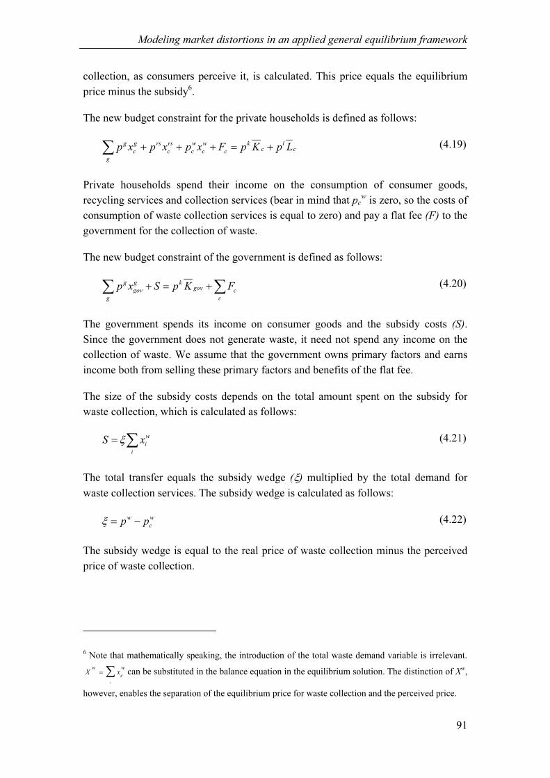
Modeling market distortions in an applied general equilibrium framework
91
collection, as consumers perceive it, is calculated. This price equals the equilibrium
price minus the subsidy6.
The new budget constraint for the private households is defined as follows:
g g rs rs w w k lc cc c c c c
g
p x p x p x F p K p L+ + + = +∑ (4.19)
Private households spend their income on the consumption of consumer goods,
recycling services and collection services (bear in mind that pc
w is zero, so the costs of
consumption of waste collection services is equal to zero) and pay a flat fee (F) to the
government for the collection of waste.
The new budget constraint of the government is defined as follows:
g g kgovgov c
g c
p x S p K F+ = +∑ ∑ (4.20)
The government spends its income on consumer goods and the subsidy costs (S).
Since the government does not generate waste, it need not spend any income on the
collection of waste. We assume that the government owns primary factors and earns
income both from selling these primary factors and benefits of the flat fee.
The size of the subsidy costs depends on the total amount spent on the subsidy for
waste collection, which is calculated as follows:
w
i
i
S xξ= ∑ (4.21)
The total transfer equals the subsidy wedge (ξ) multiplied by the total demand for
waste collection services. The subsidy wedge is calculated as follows:
w w
cp pξ = − (4.22)
The subsidy wedge is equal to the real price of waste collection minus the perceived
price of waste collection.
6 Note that mathematically speaking, the introduction of the total waste demand variable is irrelevant.
c
w w
cX x= ∑ can be substituted in the balance equation in the equilibrium solution. The distinction of Xw,
however, enables the separation of the equilibrium price for waste collection and the perceived price.

Chapter 4
92
4.2.5 Description of model including an upstream tax for waste collection
In the upstream tax model, the price of waste collection and treatment is internalized
in the price of the consumption good. Only agricultural and industrial goods are taxed,
given that the consumption of services does not generate municipal solid waste.
Introducing a tax in the Negishi format is quite similar to introducing a subsidy. First
of all the social welfare function should be adjusted. The new social welfare function
is defined as follows:
( ) max ( )
0 , 0, 0 ,
g w w g g
i i i
i g
g
i i i j
TWF u x X X
x w r all i y all j
α α ξ ξ= + +
≥ ≥ ≥
∑ ∑
(4.23)
Where ξ g is the tax wedge and X g is the total demand for good g.
Just as in Section 4.2.4, the balance constraint for the consumption goods also has to
be changed. It is important to realize that only the private households pay an upstream
tax for waste collection. Neither the producers, who demand goods as intermediate
deliveries, nor the government, who does not to generate waste, have to pay this tax.
The new balance constraints are defined as follows:
g g g g g
j gov
j
X x x y p+ + ≤ ⊥∑ (4.24)
g g g
c c
c
x X p≤ ⊥∑ (4.25)
The equilibrium price for consumption goods can be calculated from the first balance
constraint (4.24). Both the producers and the government pay this price while
consuming these goods. In the second balance constraint (4.25), the price including
the upstream tax is calculated. Only private households pay this price.
The budget constraint for private households is defined as:
g g rs rs w w k lc cc c c c c c
g
p x p x p x F p K p L+ + + = +∑ (4.26)
The budget constraint for the government is defined as:
g g kgovgov c
g c
p x S p K F T+ = + +∑ ∑ (4.27)
Where T equals the total gains of the upstream tax.

Modeling market distortions in an applied general equilibrium framework
93
4.3 A numerical example
The model discussed above is applied in a stylized example with numerical data from
the Netherlands. The economic data used in the numerical example are based on
national accounts for the Netherlands in 1996 (Statistics Netherlands, 1998). These
data are aggregated to four sectors (agricultural goods, industrial goods, services and
extraction) and two production factors (capital and labor) and supplemented with
detailed data of the waste sectors (recycled material, recycling services, collection,
incineration, landfilling, fee and subsidy) based on WMC (1998) and RIVM (1998).
To keep the model as simple as possible, we have chosen to give the government an
income dependent on capital endowments instead of an income from taxes on labor
and consumer goods7. This has been adjusted in the social accounting matrix.
4.3.1 Parameter values used in numerical example
The social accounting matrix, displayed in Table 4-1, describes the initial equilibrium.
Supply or producers’ output and consumer endowments are given positive values;
demand or producer inputs and consumption are given negative values8.
Prices are normalized to unity, except the price of waste collection9. Private
households pay 9.5 million guilders in the form of a flat fee for collection of waste.
This is slightly lower than the real cost of waste collection, which equals 10 million
guilders. This means that waste collection basically has two prices: the perceived
price and the social price of waste collection.
7 Although less realistic, we feel that it is justified to make this assumption since our focus is on waste
generation and recycling by private households. As we are interested in finding a first-best equilibrium
solution, we abstract from the existence of distortionary taxes. Therefore, in our model in makes no
difference whether the government has non-distortionary taxes as income or capital endowments.
8 The entries in the column times the corresponding prices sums up to zero to ensure that the zero profit
condition holds: value of inputs equals value of outputs. The entries in the column of each consumer
times the corresponding price sums up to zero to ensure that the budget constraint holds: each
consumer spends exactly his income on the consumption of goods and services. The entries in each row
times the corresponding prices sums up to zero to ensure that each market clears: total demand for each
commodity must equal total supply.
9 Following standard practice, we adopted the Harberger convention in the benchmark data for all
unknown prices. The Harberger convention consists of normalizing prices to unity. Quantities in the
benchmark data represent expenditures, or how much of that good or factor one can buy for €1. It
should be noted that an Arrow-Debreu economy only depends upon relative prices. Doubling all prices
doubles both money profits and income, which results in the same equilibrium outcome.
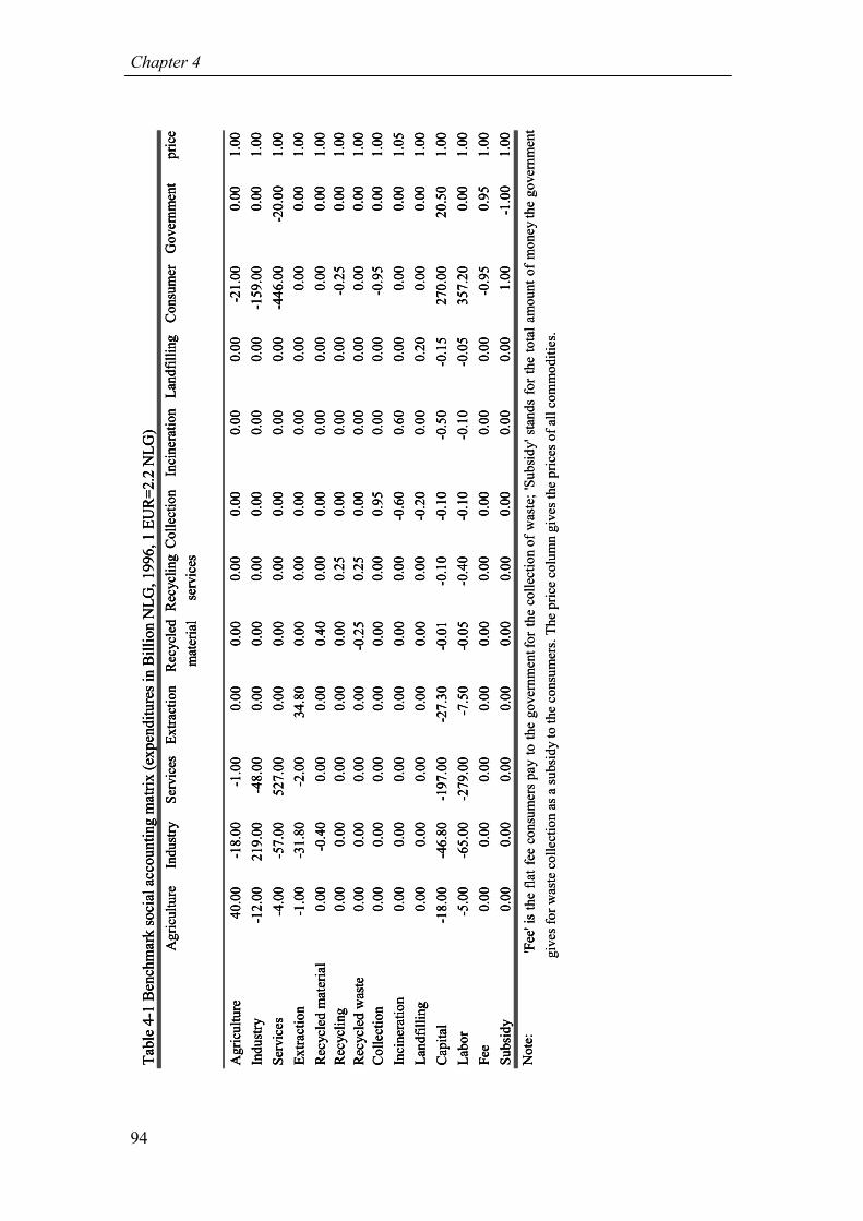
Chapter 4
94
Ag
ricu
ltu
reIn
du
stry
Ser
vic
esE
xtr
acti
on
Rec
ycl
ed
mat
eria
l
Rec
ycl
ing
serv
ices
Co
llec
tio
nIn
cin
erat
ion
Lan
dfi
llin
gC
on
sum
erG
over
nm
ent
pri
ce
Ag
ricu
ltu
re4
0.0
0-1
8.0
0-1
.00
0.0
00
.00
0.0
00
.00
0.0
00
.00
-21
.00
0.0
01
.00
Ind
ust
ry-1
2.0
02
19
.00
-48
.00
0.0
00
.00
0.0
00
.00
0.0
00
.00
-15
9.0
00
.00
1.0
0
Ser
vic
es-4
.00
-57
.00
52
7.0
00
.00
0.0
00
.00
0.0
00
.00
0.0
0-4
46
.00
-20
.00
1.0
0
Ex
trac
tio
n-1
.00
-31
.80
-2.0
03
4.8
00
.00
0.0
00
.00
0.0
00
.00
0.0
00
.00
1.0
0
Rec
ycl
ed m
ater
ial
0.0
0-0
.40
0.0
00
.00
0.4
00
.00
0.0
00
.00
0.0
00
.00
0.0
01
.00
Rec
ycl
ing
0
.00
0.0
00
.00
0.0
00
.00
0.2
50
.00
0.0
00
.00
-0.2
50
.00
1.0
0
Rec
ycl
ed w
aste
0.0
00
.00
0.0
00
.00
-0.2
50
.25
0.0
00
.00
0.0
00
.00
0.0
01
.00
Co
llec
tio
n0
.00
0.0
00
.00
0.0
00
.00
0.0
00
.95
0.0
00
.00
-0.9
50
.00
1.0
0
Inci
ner
atio
n0
.00
0.0
00
.00
0.0
00
.00
0.0
0-0
.60
0.6
00
.00
0.0
00
.00
1.0
5
Lan
dfi
llin
g0
.00
0.0
00
.00
0.0
00
.00
0.0
0-0
.20
0.0
00
.20
0.0
00
.00
1.0
0
Cap
ital
-18
.00
-46
.80
-19
7.0
0-2
7.3
0-0
.01
-0.1
0-0
.10
-0.5
0-0
.15
27
0.0
02
0.5
01
.00
Lab
or
-5.0
0-6
5.0
0-2
79
.00
-7.5
0-0
.05
-0.4
0-0
.10
-0.1
0-0
.05
35
7.2
00
.00
1.0
0
Fee
0.0
00
.00
0.0
00
.00
0.0
00
.00
0.0
00
.00
0.0
0-0
.95
0.9
51
.00
Su
bsi
dy
0.0
00
.00
0.0
00
.00
0.0
00
.00
0.0
00
.00
0.0
01
.00
-1.0
01
.00
No
te:
Tab
le 4
-1 B
ench
mar
k s
oci
al a
ccounti
ng m
atri
x (
exp
endit
ure
s in
Bil
lion N
LG
, 1996, 1 E
UR
=2.2
NL
G)
'Fee
'is
the
flat
fee
con
sum
ers
pay
toth
eg
over
nm
entfo
rth
eco
llec
tio
no
fw
aste
;'S
ub
sid
y'st
and
sfo
rth
eto
tal
amo
un
to
fm
on
eyth
eg
over
nm
ent
giv
es f
or
was
te c
oll
ecti
on
as
a su
bsi
dy t
o t
he
con
sum
ers.
Th
e p
rice
co
lum
n g
ives
th
e p
rice
s o
f al
l co
mm
od
itie
s.
Ag
ricu
ltu
reIn
du
stry
Ser
vic
esE
xtr
acti
on
Rec
ycl
ed
mat
eria
l
Rec
ycl
ing
serv
ices
Co
llec
tio
nIn
cin
erat
ion
Lan
dfi
llin
gC
on
sum
erG
over
nm
ent
pri
ce
Ag
ricu
ltu
re4
0.0
0-1
8.0
0-1
.00
0.0
00
.00
0.0
00
.00
0.0
00
.00
-21
.00
0.0
01
.00
Ind
ust
ry-1
2.0
02
19
.00
-48
.00
0.0
00
.00
0.0
00
.00
0.0
00
.00
-15
9.0
00
.00
1.0
0
Ser
vic
es-4
.00
-57
.00
52
7.0
00
.00
0.0
00
.00
0.0
00
.00
0.0
0-4
46
.00
-20
.00
1.0
0
Ex
trac
tio
n-1
.00
-31
.80
-2.0
03
4.8
00
.00
0.0
00
.00
0.0
00
.00
0.0
00
.00
1.0
0
Rec
ycl
ed m
ater
ial
0.0
0-0
.40
0.0
00
.00
0.4
00
.00
0.0
00
.00
0.0
00
.00
0.0
01
.00
Rec
ycl
ing
0
.00
0.0
00
.00
0.0
00
.00
0.2
50
.00
0.0
00
.00
-0.2
50
.00
1.0
0
Rec
ycl
ed w
aste
0.0
00
.00
0.0
00
.00
-0.2
50
.25
0.0
00
.00
0.0
00
.00
0.0
01
.00
Co
llec
tio
n0
.00
0.0
00
.00
0.0
00
.00
0.0
00
.95
0.0
00
.00
-0.9
50
.00
1.0
0
Inci
ner
atio
n0
.00
0.0
00
.00
0.0
00
.00
0.0
0-0
.60
0.6
00
.00
0.0
00
.00
1.0
5
Lan
dfi
llin
g0
.00
0.0
00
.00
0.0
00
.00
0.0
0-0
.20
0.0
00
.20
0.0
00
.00
1.0
0
Cap
ital
-18
.00
-46
.80
-19
7.0
0-2
7.3
0-0
.01
-0.1
0-0
.10
-0.5
0-0
.15
27
0.0
02
0.5
01
.00
Lab
or
-5.0
0-6
5.0
0-2
79
.00
-7.5
0-0
.05
-0.4
0-0
.10
-0.1
0-0
.05
35
7.2
00
.00
1.0
0
Fee
0.0
00
.00
0.0
00
.00
0.0
00
.00
0.0
00
.00
0.0
0-0
.95
0.9
51
.00
Su
bsi
dy
0.0
00
.00
0.0
00
.00
0.0
00
.00
0.0
00
.00
0.0
01
.00
-1.0
01
.00
No
te:
Tab
le 4
-1 B
ench
mar
k s
oci
al a
ccounti
ng m
atri
x (
exp
endit
ure
s in
Bil
lion N
LG
, 1996, 1 E
UR
=2.2
NL
G)
'Fee
'is
Ag
ricu
ltu
reIn
du
stry
Ser
vic
esE
xtr
acti
on
Rec
ycl
ed
mat
eria
l
Rec
ycl
ing
serv
ices
Co
llec
tio
nIn
cin
erat
ion
Lan
dfi
llin
gC
on
sum
erG
over
nm
ent
pri
ce
Ag
ricu
ltu
re4
0.0
0-1
8.0
0-1
.00
0.0
00
.00
0.0
00
.00
0.0
00
.00
-21
.00
0.0
01
.00
Ind
ust
ry-1
2.0
02
19
.00
-48
.00
0.0
00
.00
0.0
00
.00
0.0
00
.00
-15
9.0
00
.00
1.0
0
Ser
vic
es-4
.00
-57
.00
52
7.0
00
.00
0.0
00
.00
0.0
00
.00
0.0
0-4
46
.00
-20
.00
1.0
0
Ex
trac
tio
n-1
.00
-31
.80
-2.0
03
4.8
00
.00
0.0
00
.00
0.0
00
.00
0.0
00
.00
1.0
0
Rec
ycl
ed m
ater
ial
0.0
0-0
.40
0.0
00
.00
0.4
00
.00
0.0
00
.00
0.0
00
.00
0.0
01
.00
Rec
ycl
ing
0
.00
0.0
00
.00
0.0
00
.00
0.2
50
.00
0.0
00
.00
-0.2
50
.00
1.0
0
Rec
ycl
ed w
aste
0.0
00
.00
0.0
00
.00
-0.2
50
.25
0.0
00
.00
0.0
00
.00
0.0
01
.00
Co
llec
tio
n0
.00
0.0
00
.00
0.0
00
.00
0.0
00
.95
0.0
00
.00
-0.9
50
.00
1.0
0
Inci
ner
atio
n0
.00
0.0
00
.00
0.0
00
.00
0.0
0-0
.60
0.6
00
.00
0.0
00
.00
1.0
5
Lan
dfi
llin
g0
.00
0.0
00
.00
0.0
00
.00
0.0
0-0
.20
0.0
00
.20
0.0
00
.00
1.0
0
Cap
ital
-18
.00
-46
.80
-19
7.0
0-2
7.3
0-0
.01
-0.1
0-0
.10
-0.5
0-0
.15
27
0.0
02
0.5
01
.00
Lab
or
-5.0
0-6
5.0
0-2
79
.00
-7.5
0-0
.05
-0.4
0-0
.10
-0.1
0-0
.05
35
7.2
00
.00
1.0
0
Fee
0.0
00
.00
0.0
00
.00
0.0
00
.00
0.0
00
.00
0.0
0-0
.95
0.9
51
.00
Su
bsi
dy
0.0
00
.00
0.0
00
.00
0.0
00
.00
0.0
00
.00
0.0
01
.00
-1.0
01
.00
No
te:
Tab
le 4
-1 B
ench
mar
k s
oci
al a
ccounti
ng m
atri
x (
exp
endit
ure
s in
Bil
lion N
LG
, 1996, 1 E
UR
=2.2
NL
G)
'Fee
'is
the
flat
fee
con
sum
ers
pay
toth
eg
over
nm
entfo
rth
eco
llec
tio
no
fw
aste
;'S
ub
sid
y'st
and
sfo
rth
eto
tal
amo
un
to
fm
on
eyth
eg
over
nm
ent
giv
es f
or
was
te c
oll
ecti
on
as
a su
bsi
dy t
o t
he
con
sum
ers.
Th
e p
rice
co
lum
n g
ives
th
e p
rice
s o
f al
l co
mm
od
itie
s.

Modeling market distortions in an applied general equilibrium framework
95
The perceived price equals the total fee divided by the total demand for waste
collection. The social price equals the total fee plus the total amount paid by the
municipality for waste collection divided by total demand. We have chosen to
normalize the perceived price of waste collection, which means that the social price
for waste collection (which is shown in Table 4.1) is higher than unity.
All production sectors are characterized by a CES production function. As mentioned
earlier, all production sectors use capital and labor. The substitution elasticity between
capital and labor equals 0.8, based on the study by Draper and Manders (1996). Other
substitution elasticities are presented in Table 4-2. The three production sectors of
consumer goods (agriculture, industry and services) also use intermediate inputs for
production. The use of primary factors and intermediate inputs is strictly
complementary. Only the producer of industrial goods uses recycled material. They
can fully substitute recycled for virgin materials.
Table 4-2 Substitution elasticities for the production sectors
Agriculture Industry Services Recycled
Material
Collection
Sub.elas. primary &
intermediate inputs (σpi)
0.0 0.0 0.0 - -
Sub.elas. materials &
intermediate inputs (σwm
)
1.0 1.0 1.0 - -
Sub.elas. recycled material
& virgin material (σvr
)
- ∞ - - -
Sub.elas. primary factors
& recycled waste (σpr
)
- - - 0.125 -
Sub.elas. landfilling &
incineration (σil)
- - - - 0.2
The substitution parameters for the households are shown in Table 4-3. Utility of the
private households depends on consumption of agricultural goods, industrial goods,
and services. A substitution elasticity of unity between goods is assumed (Cobb-
Douglas utility function). The government only consumes services and thus has no
substitution elasticity between consumption goods.
Table 4-3 Additional parameters for households in the benchmark
Consumer Government
Substitution elasticity between consumer goods (σ g) 1.0
Negishi weights (α) 96.9 3.1
The initial Negishi weights are determined on the basis of the initial income (sales of
endowments). Since the income of the private households is far greater than the
income of the government, the Negishi weight of the private households is much
larger.

Chapter 4
96
In the base case scenario, collection and treatment of municipal solid waste costs
about 1.2 Billion guilders. Consuming either agricultural goods or industrial goods
generates waste. One unit of agricultural goods contains a smaller percentage of waste
than industrial goods. The percentage of waste present in a unit of agricultural goods
is equal to 0.46 and the percentage of waste present in a unit of industrial goods is
equal to 0.69. Of the waste generated, about 20% is recycled and 80% collected for
waste treatment (either landfilling or incineration). Most of the waste collected is
incinerated (75%); the rest is landfilled.
4.3.2 Policy scenarios
The model specified in the previous section is used to analyze the effects of different
policy options, especially on the quantity of solid waste generated and the total costs
of waste treatment. In this chapter, four policy instruments are compared, namely
unit-based pricing of waste collection, recycling subsidy, unit-based pricing of waste
collection combined with a recycling subsidy and an upstream tax. Seven different
scenario’s are distinguished: (i) unit-based price, (ii) recycling subsidy (iii) unit-
based price plus recycling subsidy (iv) upstream tax, (v) unit based price plus
transaction costs, (vi) unit based price plus recycling subsidy plus transaction costs
and (vii) upstream tax plus transaction costs.
The benchmark case is an exact replication of the benchmark data presented in section
4.3.1 without added policies. The seven scenarios will all be compared with the
benchmark case.
In the first scenario, the flat fee-pricing scheme is replaced by a unit-based pricing
scheme. The private households now bear the full costs of waste collection, whereas
in the flat fee pricing system, consumers only had to pay 95% of the total costs. This
scenario is labeled the ‘unit-based price scenario’.
According to the second scenario, recycling is promoted by lowering the cost of
producing recycling services, i.e. production costs for recycling are halved, and thus
the benchmark price for recycling services is halved. The flat pricing scheme remains
unchanged. This policy is labeled the ‘recycling subsidy scenario’.
In the third scenario, the unit-based pricing scheme is combined with a recycling
subsidy. As shown in Chapter 2, the unit-based pricing scheme is usually
implemented together with policies intended to stimulate recycling. Therefore, in this
scenario both policy options are implemented together.
A small upstream tax on agricultural and industrial goods is introduced in the fourth
scenario. This tax internalizes the cost of waste collection and treatment in the price of
the product. The private households do not have to pay anything for the collection of
waste. This scenario is labeled the ‘upstream tax scenario’.

Modeling market distortions in an applied general equilibrium framework
97
In the fifth scenario, the unit-based pricing system is introduced once again. In this
scenario, however, some transaction costs of introducing a unit-based price are
included. These transaction cost may involve the costs of installing weighing scales in
garbage trucks and costs incurred as a consequence of preventing illegal disposal. By
changing the available technology (A) in the production function, we introduced
transaction costs. It is here assumed that a more expensive technology has to be used,
which means that less output can be generated with the same amount of input. This
scenario is labeled the ‘unit-based price plus transaction costs scenario’.
In the sixth scenario, the unit based pricing system and recycling subsidy is combined
with the transaction costs involved in implementing such a policy change. Transaction
costs are implemented in the same manner as in scenario five.
In the seventh and final scenario, the upstream tax is combined with transaction costs
of introducing an upstream tax. We assume that all transaction costs will be borne by
the consumers. This means that the tax will be higher than in the ‘upstream tax
scenario’. This scenario is labeled the ‘upstream tax plus transaction costs scenario’.
The different elements of each scenario are summarized in Table 4-4.
Table 4-4 Main characteristics of the policy scenarios
Scenario Fee collection Tax or subsidy Transaction costs
Benchmark case Flat fee No No
1. Unit-based price Unit-based fee No No
2. Recycling subsidy Flat fee Subsidy No
3. Unit-based price + recycling
subsidy
Unit-based price Subsidy No
4. Upstream Tax No fee Tax No
5. Unit-based price + transaction
costs
Unit-based fee No Yes
6. Unit-based price + recycling
subsidy + transaction costs
Unit-based fee Subsidy Yes
7. Upstream tax + transaction costs No fee Tax Yes
4.3.3 Results
First scenario: Unit-based pricing scheme scenario
In the first scenario, a unit-based pricing scheme is introduced. Households pay the
equilibrium price for waste collection. This means that generating more waste will
result in higher collection costs. Table 4-5 shows the changes in the main variables of
the model. The government no longer bears the costs of collection. This means that
the relative income that can be used for the consumption of services increases.
Therefore, to keep government expenditure constant, as discussed in Section 4.3.1,
private households receive a positive lump-sum transfer from the government. Private

Chapter 4
98
households now bear the full cost of waste collection, but due to the positive lump-
sum transfer there is small change in their available income.
Table 4-5 The main variables for the ‘Unit-based pricing scenario’ as compared to the
‘Benchmark case’ (expenditures in Billion NLG, 1996) and the percentage change
Variable Benchmark
case
Unit-based price % Change
Private demand agricultural good 21.00 20.94 (-0.27%)
Private demand industrial good 159.00 158.18 (-0.52%)
Private demand services 446.00 446.89 (0.20%)
Private demand recycling services 0.25 0.26 (6.65%)
Private demand waste collection 0.95 0.93 (-2.38%)
Utility private households 309.77 309.78 (0.00%)
Households are given an incentive to prevent waste and recycle more. They substitute
agricultural and industrial goods, which contain relative large quantities of waste, for
services, which do not contain waste. Since the perceived price for waste collection
has risen, there is some substitution between recycling and waste collection. Demand
for recycling services increases and the demand for collection services decreases.
Since the consumer’s income is hardly affected by the policy change, the utility of the
private households remains almost unchanged.
Second scenario: Recycling subsidy
In the second scenario, the production costs of recycling are reduced. This is done by
introducing a new technology parameter in the production set, which makes it
possible to produce the same quantity of recycling services with the use of less
production factors. Table 4-6 shows the changes of the most important variables.
Table 4-6 The main variables for the ‘Recycling subsidy scenario’ as compared to the
‘Benchmark case’ (expenditures in Billion NLG, 1996) and the percentage change
Benchmark
case
Recycling
subsidy
% Change
Private demand agricultural good 21.00 21.00 (0.019%)
Private demand industrial good 159.00 159.04 (0.025%)
Private demand services 446.00 446.12 (0.027%)
Private demand recycling services 0.25 0.25 (0.000%)
Private demand waste collection 0.95 0.95 (0.031%)
Utility private households 309.77 309.85 (0.026%)
The change in most variables is very small. Since the quantity of recycling is quite
small according to the benchmark, the effects of lower recycling costs will also be
fairly minimal. The demand for recycling services is unaffected by the lower price for
recycling services. This is a logical result because if consumers have the choice
between collection and recycling services, they will chose collection, which is free.

Modeling market distortions in an applied general equilibrium framework
99
Thus, a lower price for recycling services does not affect the demand for these
services as long as this price is larger than zero. The demand for waste collection rises
slightly since the consumer can consume more goods since they have to spend less
income on recycling.
The utility of the private consumers rises slightly, because lower recycling costs imply
that a larger percentage of the income can be spent on consumer goods. The money
that the government spends on the subsidy is slightly increased, as the consumers
demand more waste collection services. Since the expenditure of the government is
kept constant at the benchmark level (see Section 4.3.1), this means that the
government will receive a small lump-sum transfer from the private households to
compensate for the extra costs.
Third scenario: Unit-based price plus recycling subsidy scenario
In the third scenario, both the unit-based price for waste collection and the lower price
for recycling services are introduced simultaneously. Consumers are given a strong
price incentive to demand more recycling services and less waste collection services
(see Table 4-7). Recycling increases strongly, and waste collection decreases by more
than 70%. Due to the lower costs for waste treatment, consumption and utility of the
private households increase slightly. Compared to the recycling subsidy scenario,
utility of the private households increases more than twice as much.
Table 4-7 Changes in the main variables for the ‘Unit-based price and recycling
subsidy scenario’ as compared to the ‘Benchmark case’ (expenditures in Billion NLG,
1996) and the percentage change.
Benchmark
case
Unit-based price and
recycling subsidy
% Change
Private demand agricultural good 21.00 20.97 (-0.14%)
Private demand industrial good 159.00 158.46 (-0.34%)
Private demand services 446.00 446.94 (0.21%)
Private demand recycling services 0.25 0.92 (266.55%)
Private demand waste collection 0.95 0.28 (-70.56%)
Utility private households 309.77 309.96 (0.06%)
Scenario two and three demonstrate the impact of policies aimed at promoting
recycling under different pricing schemes for waste collection. Under the flat fee-
pricing scheme, promoting recycling is not effective. Consumption rises, waste
generation rises and waste collection rises; the exact opposite of the goal of the policy
change. In scenario three, however, the quantity of waste generated decreases. More
waste is recycled and less waste is collected, incinerated, and landfilled.
A comparison of these scenarios reveals that in the case of a flat fee for waste
collection, the market is distorted and the price of recycling has no impact on the

Chapter 4
100
behavior of households. The unit-based price is far more effective when combined
with a recycling subsidy. This is in line with the results of actual practice;
municipalities always introduce a unit-based pricing scheme in combination with
policies promoting recycling.
Fourth scenario: Upstream tax scenario
An upstream tax is introduced in the fourth scenario. The tax is quite small and is only
intended to cover the real cost of waste collection. Since the consumption of
agricultural goods and industrial goods leads to waste generation, these two goods are
taxed.
Table 4-8 The main variables for the ‘Upstream tax scenario’ as compared to the
‘Benchmark case’ (expenditures in Billion NLG, 1996) and the percentage change.
Variable Benchmark
case
Upstream tax % Change
Private demand agricultural good 21.00 20.96 (-0.21%)
Private demand industrial good 159.00 158.34 (-0.41%)
Private demand services 446.00 446.71 (0.16%)
Private demand recycling services 0.25 0.25 (-0.04%)
Private demand waste collection 0.95 0.95 (-0.49%)
Utility private households 309.77 309.78 (0.00%)
The results of the upstream tax scenario are shown in Table 4-8. Since households pay
a higher price for agricultural goods and industrial goods, the demand for these goods
declines. The demand for services increases, because the price of services has not
been affected. Given that fewer agricultural and industrial goods are consumed, the
quantity of waste generated decreases slightly. The utility of the consumers is hardly
affected by the measure. Compared with the ‘unit-based price scenario’, it is clear that
the up-stream tax is less effective in minimizing the waste problem. Moreover, there
is no substitution of recycling for collection.
Fifth scenario: Unit-based price plus transaction costs scenario
A frequent complaint about the unit-based pricing scheme is the huge transaction
costs of introducing such a scheme. In most models, these costs are left out of the
analysis. In the fifth scenario both the unit based pricing scheme and transaction costs
of introducing such a scheme have been included. To cover these extra costs, private
households will have to pay a higher fee compared to the unit-based pricing scenario.
In Table 4-9 the results of third scenario are presented. Consumption has slightly
decreased due to the increase of waste disposal costs. Private households must spend
more income on waste disposal and thus have less money available for consumption.
Since the costs of waste collection have increased, consumers begin to recycle more

Modeling market distortions in an applied general equilibrium framework
101
waste. Compared with scenario 1, more waste is recycled, while the utility of both the
private households and the government is lower.
Table 4-9 The main variables for the ‘unit-based price plus transaction costs’ as
compared to the ‘Benchmark case’ (expenditures in Billion NLG, 1996) and the
percentage change
Variable Benchmark
case
Unit-based price +
transaction costs
% Change
Private demand agricultural good 21.00 20.93 (-0.31%)
Private demand industrial good 159.00 158.08 (-0.58%)
Private demand services 446.00 446.90 (0.20%)
Private demand recycling services 0.25 0.31 (25.45%)
Private demand waste collection 0.95 0.88 (-7.40%)
Utility private households 309.77 309.73 (-0.02%)
Implementing a unit-based pricing scheme seems inefficient based on the results
presented in Table 4-9. No government should implement a policy that lowers the
total welfare of the country. However, it is important to bear in mind that
environmental damage is not included in the model. Collection and treatment of waste
leads to environmental damage. Recycling, on the other hand, results in far less
environmental damage. If the state of the environment was to be included in the social
welfare function, it may well be that this policy scenario performs relatively well in
terms of an increase in social welfare.
Sixth scenario: Unit-based price plus recycling subsidy plus transaction costs
scenario
The unit based pricing scheme, recycling subsidy, and transaction costs of introducing
such a scheme are included in the sixth scenario. The transaction costs are
implemented in the same way as in the fifth scenario; consumers bear all transaction
costs. The results of this scenario are shown in Table 4-10.
Table 4-10 The main variables for the ‘Unit-based price plus recycling subsidy plus
transaction costs’ as compared to the ‘Benchmark case’ (expenditures in Billion NLG,
1996) and the percentage change.
Variable Benchmark
case
Unit-based price +
recycling subsidy +
transaction costs
% Change
Private demand agricultural good 21.00 20.97 (-0.13%)
Private demand industrial good 159.00 158.45 (-0.34%)
Private demand services 446.00 446.57 (0.21%)
Private demand recycling services 0.25 11.96 (378.38%)
Private demand waste collection 0.95 0.00 (-99.99%)
Utility private households 309.77 309.73 (0.06%)

Chapter 4
102
We assumed that there are no technical restrictions on recycling of waste, therefore in
theory it is possible to recycle all waste that is generated. Although this assumption is
not completely realistic, the main objective of this chapter is to demonstrate the main
mechanisms of the model. Due to the increased price of waste collection services and
the low costs of recycling, consumers start to recycle almost all their rest waste. Since
recycling is cheaper than waste collection, they are able to spend a larger part of their
income on the consumption of goods, thus their utility increases. Shifting
consumption from agricultural and industrial goods to services prevents some of the
waste. Compared to scenario five, more agricultural goods and industrial goods and
about the same quantity of services are consumed.
Seventh scenario: Upstream tax plus transaction costs scenario
In the seventh scenario, an upstream tax on consumption goods is introduced. We
assume that all transactions costs of introducing such a tax will be borne by the
private households. This means that transaction costs may be introduced by increasing
the total tax. This tax is slightly higher than in scenario 2, to cover the transaction
costs.
Table 4-11 The main variables for the ‘Upstream tax scenario plus transaction costs’
as compared to the ‘Benchmark case’ (expenditures in Billion NLG, 1996) and the
percentage change.
Benchmark
case
Upstream tax +
transaction costs
% Change
Private demand agricultural good 21.00 20.95 (-0.26%)
Private demand industrial good 159.00 158.24 (-0.48%)
Private demand services 446.00 446.71 (0.16%)
Private demand recycling services 0.25 0.25 (-0.04%)
Private demand waste collection 0.95 0.95 (-0.57%)
Utility private households 309.77 309.72 (-0.02%)
In Table 4-11, the results of this scenario are presented. The higher tax does not
change the results too greatly. Somewhat less waste is generated. The demand for
agricultural goods and industrial goods decreases slightly and the demand for
services, the only good without a tax, increases. These results indicate a minor
decrease in the demand for both recycling services and collection services. Due to the
costs of implementing the tax, the utility of both consumers decreases.
4.3.4 Sensitivity analysis
Substitution elasticity between consumer goods
The effectiveness of the upstream tax and, to a lesser extent, the unit-based pricing
scheme depends on the substitution elasticity between consumption goods. If the
demand for consumption goods is more elastic it can be expected that consumers will

Modeling market distortions in an applied general equilibrium framework
103
substitute more industrial and agricultural goods for services. A sensitivity analysis is
performed for the substitution elasticity between the consumption goods. The
substitution elasticity is changed from low to high in a number of (equidistant) steps,
resulting in a very inelastic demand to an elastic demand. The effects of parameter
changes on the variables: rest waste and recyclable waste are calculated.
Figure 4-3 shows the impact of the substitution elasticity on the generation of rest
waste, which is collected by the municipality.
0.86
0.88
0.9
0.92
0.94
0.96
0.3 0.4 0.5 0.6 0.7 0.8 0.9 1 1.1 1.2 1.3 1.4 1.5 1.6 1.7 1.8 1.9
Index of subst. elas. values and benchmark value
(Benchmark=1)
Res
t w
aste
(ex
pen
dit
ure
in
Bil
lion N
LG
)
0.277
0.278
0.278
0.279
0.280
0.280
0.281
Res
t w
aste
in u
nit
pri
ce +
subsi
dy s
cenar
io
Upstream tax
Upstream tax
+ transaction
Unit price
Unit price +
transaction
Unit price +
subsidy
Figure 4-3 Sensitivity analysis of the substitution elasticity between different
consumption goods: impacts on the generation of rest waste
Figure 4-3 does not include the scenario unit-based price plus recycling subsidy plus
transaction costs as in this scenario all waste is recycled independent of the
substitution elasticity between consumption goods. For each scenario, the demand for
waste collection is slightly sensitive to the substitution elasticity. If the demand for
consumption goods is elastic, private households will substitute agricultural and
industrial goods by services and generate less waste. Figure 4-3 demonstrates that the
unit-based pricing scheme is more effective in reducing waste generation than the
upstream tax10
.
The demand for recycling services is barely affected by changes in the substitution
elasticity, which is shown in Figure 4-4.
10 The value of the substitution elasticity is calculated as the value of the benchmark substitution
elasticity multiplied by a certain factor, where the value of the factor is shown on the x-axis.

Chapter 4
104
0.24
0.26
0.28
0.3
0.32
0.34
0.3 0.4 0.5 0.6 0.7 0.8 0.9 1 1.1 1.2 1.3 1.4 1.5 1.6 1.7 1.8 1.9
Index of sub. elas. between different consumption goods
(benchmark=1)
Rec
ycl
able
was
te (
expen
dit
ure
in
Bil
lion N
LG
)
0.9
0.904
0.908
0.912
0.916
0.92
Rec
yca
ble
was
te i
n u
nit
pri
ce +
subsi
dy
sce
nar
io
Unit price +
transaction
Unit price
Upstream
tax
Unit price +
subsidy
Figure 4-4 Sensitivity analysis of the substitution elasticity between different
consumption goods: impacts on the generation of recyclable waste
A unit-based price provides households with an incentive to increase recycling. If less
waste is generated, however, recycling will also slightly decline. An upstream tax
stimulates private households to generate less waste, but does not stimulate recycling.
Therefore, the demand for recycling services is not affected and remains at benchmark
level for both the upstream tax scenario as the upstream tax plus transaction costs
scenario. As the results are identical for these scenarios, only the results for the
upstream tax scenario have been displayed in Figure 4-4.
Transaction costs
The total costs of implementing a policy will greatly determine the effectiveness of
that policy. In the scenarios presented earlier, it was assumed that transaction costs
would increase collection costs by 11%. The transaction costs, however, can also be
far higher. To analyze how sensitive the results are, the transaction costs have been
increased from benchmark level (100%) by 2.5 times as much. The results for the
total quantity of waste generated, i.e. both recyclable waste and rest waste, are
presented in Figure 4-5.
As can be seen from Figure 4-5, the upstream tax is more efficient in preventing waste
than the unit-based price. Figure 4-5 demonstrates that if the transaction costs are
large levying an upstream tax will prevent more waste than levying a unit-based price.
The unit-based price combined with a recycling subsidy does not help the prevention
of waste. The unit-based price, however, not only stimulates waste prevention but also
waste recycling, as shown in Figure 4-6.

Modeling market distortions in an applied general equilibrium framework
105
1.184
1.186
1.188
1.19
1.192
1.194
1.196
1.198
100% 111% 125% 143% 167% 200% 250%
Index of transaction costs
(benchmark=100%)
Was
te g
ener
ated
(ex
pen
dit
ure
in
Bil
lion N
LG
)
Unit-based
price +
subsidy
Unit-based
price
Upstream
tax
Figure 4-5 Sensitivity analysis of the transaction costs of implementing policy:
impacts on the generation of total waste
The results for the individual categories: waste recycling and waste collection are
shown in Figure 4-6. The larger the transaction costs become, the more waste will be
recycled in the unit-based price scenario. If the costs become very large, all waste
generated will be recycled.
0
0.2
0.4
0.6
0.8
1
1.2
100% 111% 125% 143% 167% 200% 250%
Index transaction costs (benchmark=100%)
Was
te g
ener
ated
(ex
pen
dit
ure
in
Bil
lio
n N
LG
)
Unit price + subsidy --
recycling
Upstream tax--
collection
Unit-based price--
collection
Unit-based price--
recycling
Upstream tax--
recycling
Unit price + subsidy--
collection
Figure 4-6 Sensitivity analysis of the transaction costs: impacts on the generation of
recyclable waste and rest waste
Finally, the effects on the utility of the private households are shown in Figure 4-7.
The effects on utility are nearly equal for both the unit-based price policy as the
upstream tax policy if the transaction costs are small. However, if transaction costs

Chapter 4
106
increase, the upstream tax will have a far greater negative effect on the utility than the
unit-based pricing scheme. If the transaction costs become too large in the unit-based
pricing scheme, the private households will start to recycle all their waste, thereby
eliminating all costs connected to the collection of waste. In the unit-based price
scenario plus recycling subsidy, recycling is so cheap that all waste will be recycled
and thus total consumption and utility will not be affected.
308
309
309
309
309
309
310
310
310
310
100% 111% 125% 143% 167% 200% 250%
Index of transaction costs (benchmark=100%)
Uti
lity
(B
illi
on N
LG
) .
Unit-based
price
Upstream tax
Unit-based
price +
subsidy
Figure 4-7 Sensitivity analysis of the transaction costs: impacts on the utility of the
private households
4.4 Conclusions
In this chapter, we have demonstrated how a simple model simulating the waste
market and incorporating market distortions can be built using an applied general
equilibrium framework. One of the characteristics of the waste market is a flat fee-
pricing scheme for waste collection. In such a pricing scheme, the marginal costs, or
the price for waste collection as perceived by consumers equal zero. Special attention,
therefore, has been given to modeling goods with a zero price. Introducing such a
market distortion has strong effects on the results of the model. This was
demonstrated by the application of the model in a numerical example.
Flat fee pricing for waste collection leads to the inefficiently high generation of waste.
The effects of four waste management policies have been analyzed, i.e. a unit-based
pricing scheme, recycling subsidy, unit-based pricing scheme combined with
recycling subsidy and an upstream tax. The results show that a flat fee-pricing scheme
for waste collection takes away the incentive to recycle. As long as a flat fee-pricing
scheme is used, the private households do not have a price-incentive to reduce waste
generation and thus households will show little tendency to increase recycling.

Modeling market distortions in an applied general equilibrium framework
107
Making recycling more attractive by reducing the costs of recycling does not
necessarily result in less waste generated. On the contrary, lower recycling costs result
in the generation of more waste, due to the income effects of lower recycling costs.
Only if policies promoting recycling are combined with a unit-based pricing scheme
for waste collection will these policies be effective.
The results of the model clearly demonstrate that the unit-based pricing scheme is
effective in providing consumers with an incentive to recycle and prevent waste,
especially when combined with a recycling subsidy. In contrast to an upstream tax,
the unit-based price offers consumers an incentive to both recycle and prevent waste.
The upstream tax can stimulate the private households to generate less waste if the
demand for consumption goods is elastic. The upstream tax will not promote waste
recycling, but only waste prevention because recycling still has a positive marginal
price whereas collection has a zero marginal one. If the demand is inelastic, the policy
change will have barely any effect.
Both a unit-based pricing scheme and an upstream tax will, however, also negatively
affect utility and social welfare. Especially if transaction costs are considered, both
utility of the private consumers and social welfare will be negatively affected. If the
environmental gains of waste prevention and increased recycling are not large enough
to offset the decrease in utility, neither policy option should be implemented.
Different polices have been compared in this chapter using a relatively simple
example. For a more detailed assessment of waste management policies in the
Netherlands, more data must be gathered. Also modeling issues, such as including
environmental impacts and substitution possibilities between products within a sector,
should be resolved.
In this analysis, it was assumed that the private households would pay all transaction
costs of introducing a policy. In reality this may not be possible. Particularly the
social costs of illegal disposal and the costs of preventing illegal disposal may render
the unit-based pricing scheme less desirable than an upstream tax. Policy makers,
however, should bear in mind that the upstream tax is far less efficient, especially
since it does not stimulate consumers to start recycling waste.

Chapter 4
108
Appendix 4-A: Solving a Negishi format
The Negishi model calculates the equilibrium through an iterative process. First the
equilibrium is determined by solving the maximization model
( , , )i i i i i
i
TW Max u x r wα= ∑ (E.1)
Subject to the balance constraint:
,
g
i i i i j
i g i i i j
x r w y pω+ + ≤ + ⊥∑∑ ∑ ∑ ∑ ∑ (E.2)
The Negishi weights are initialized as follows:
i
i
i
i
h
hα =
∑
(E.3)
This means that the Negishi weight of consumer i is determined by the initial share this
consumer has in total income. If the share of consumer i in total income is large, the Negishi
weight of that consumer is large and vice versa. It is assumed that the utility functions of both
consumers are homothetic and commodity endowments are strictly proportional.
Homothesticity ensures that the composition of a utility maximizing commodity is unaffected
by the level of income. Due to this assumption, the social demand, i.e. the sum of individual
demands, is proportional to the level of the total income, independent of its distribution. The
competitive equilibrium prices and, therefore, the resulting allocation of resources is
independent of income distribution. Thus, the problem of income distribution is assumed
away (Negishi, 1972).
After the model is solved, the shadow price of each commodity is calculated. These shadow
prices are used to calculate the income deficit of each consumer, i.e. the difference between
total income and total expenditure of each consumer, labeled ‘loss’.
g
i i i i i
i
loss p px pr pwω= − + +∑ (E.4)
If the loss for each consumer equals zero, the equilibrium solution is found. If the loss for one
or more consumers is not equal to zero then the Negishi weights are adjusted as follows
(Ginsburgh and Keyzer, 1997):
i
i i
i
i
loss
hα α β= +
∑
(E.5)
For example, if a consumer has a surplus income, i.e. her income is larger than her
expenditure, the Negishi weight will be increased. In the next iteration, the consumption of
this consumer will be larger due to the larger Negishi weight. This iterative procedure results
in a set of unique equilibrium Negishi weights and prices.

Modeling market distortions in an applied general equilibrium framework
109
Appendix 4-B Definition of model indices, parameters, and variables
Indices
Label Entries Description
c 1 Private households
g 1...3 goods (agriculture, industry and services)
h 1,2 material (recycled and virgin)
i 1,2 Consumers (private households and government)
j 1...8 goods and services
n 1,2 waste treatment services (incineration and landfilling)
z 1...10 commodities (goods, services, capital and labor)
Parameters
Symbol Description
α Negishi weight
β waste percentage
σkl
substitution elasticity between labor and capital
σ pi substitution elasticity between primary and intermediate inputs
σ wm substitution elasticity between materials and other intermediate inputs
σ vr substitution elasticity between virgin and recycled material
σ pw substitution elasticity between primary factors and waste treatment
services
σ il substitution elasticity between incineration and landfilling services
ξ subsidy wedge
A technology parameter
F flat fee for waste collection
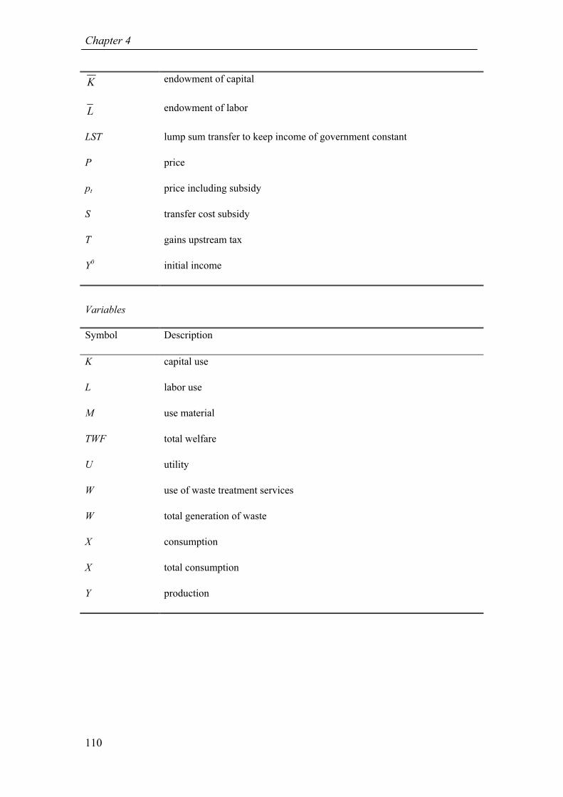
Chapter 4
110
K endowment of capital
L endowment of labor
LST lump sum transfer to keep income of government constant
P price
pt price including subsidy
S transfer cost subsidy
T gains upstream tax
Y0 initial income
Variables
Symbol Description
K capital use
L labor use
M use material
TWF total welfare
U utility
W use of waste treatment services
W total generation of waste
X consumption
X total consumption
Y production

111
5 Economic incentives and the quality of municipal solid
waste: counterproductive effects through ‘waste leakage’
5.1 Introduction
Economic literature suggests that externalities should be internalized by means of
Pigovian taxation. The costs of treating waste generated by households, which can be
seen as an externality of consumption, are not normally internalized in the price of
waste collection. Most municipalities charge a fixed amount of money, the so-called
flat fee, for the collection of waste. They tend to choose this pricing system because of
its simplicity and low transaction costs. Unfortunately, this pricing system does not
provide incentives to minimize waste generation. Since the price is fixed, marginal
costs of waste generation equal zero. A better pricing system would be a variable
price for waste collection, which is dependent on the actual amount of waste
generated, the so-called unit-based price.
Recent studies have demonstrated that the introduction of a unit-based fee contributes
to the solution of the solid waste problem, providing that due care is taken to prevent
illegal forms of disposal, such as dumping and illegal burning (see, for example,
Jenkins, 1993; Fullerton and Kinnaman, 1995, 1996; Palmer and Walls, 1997;
Fullerton and Wu, 1998 and Choe and Frasier, 1999). Disposal taxes also provide an
incentive for producers to make efficient choices about the degree of packaging, the
weight and material input of the product, and finally its rate of recyclability (Fullerton
and Wu, 1998). Municipalities throughout the world have experimented with the use
of unit-based pricing schemes for waste collection. Results of these experiments can
be found in, for example, Miranda et al. (1994), Sterner and Bartelings (1999), and
Linderhof et al. (2001).
A unit-based pricing scheme is usually implemented for the collection of rest waste
and sometimes for the collection of organic waste also. This pricing scheme is
generally accompanied with policies for the separation of organic waste and the
promotion of paper, glass, tin, and battery recycling. Research in the United States
suggests that a unit-based price is far less successful if introduced without these
recycling policies (Miranda et al., 1994). The results in Chapter 4 also support this.
Recent studies (e.g. Fullerton and Kinnaman, 1995 and Fullerton and Wu, 1998) have
focused on the possibility of illegal disposal as a consequence of introducing a unit-
based pricing system for waste collection. However, they failed to recognize another
potential problem, namely the possibility of the ‘pollution’ of recyclable or organic

Chapter 5
112
waste. Households not only have the option of burning or illegally dumping trash, but
they can also get rid of it in small amounts by putting it, for example, in organic waste
bins or glass containers, both of which are collected free of charge. This kind of waste
leakage can have serious effects. It will greatly increase the costs of recycling
‘polluted’ waste, since the recyclable waste has to be cleaned first. In the case of
organic waste, the results are even worse. Heavily ‘polluted’ organic waste can no
longer be composted. The quality of compost made from cleaned ‘polluted’ waste is
too low. As a result, composting units do not accept this ‘polluted’ waste, but instead
send it to an incinerator. This could eventually lead to all organic waste being
incinerated or landfilled.
In the Netherlands, municipalities are obliged to collect organic waste and rest waste
separately. Several large municipalities, however, have been granted an exemption
from this obligation. The quality of organic waste collected in these municipalities
was not good enough to be composted and thus it was not efficient to collect organic
waste in large parts of these municipalities (WMC, 2003e). This suggests that waste
leakage is a particular problem in larger municipalities.
Monitoring and preventing waste leakage is costly. Organic waste is usually collected
in large garbage trucks where all waste is thrown together. This makes it difficult to
distinguish the waste of one household from that of another. To locate the source of
polluted organic waste, the quality of organic waste has to be checked during
collection. This entails large transaction costs.
In this chapter, a general equilibrium model has been built to analyze the problem of
waste leakage. We only focus on waste leakage effects for the organic waste stream,
given that these effects are likely to present the most serious problems. The model
structure, however, is such that it can easily be extended to include other waste
streams, like paper and glass. Although this chapter focuses on waste leakage in a
unit-based pricing system, waste leakage is potentially a problem in any system in
which consumers are penalized for generating rest waste and rewarded for generating
recyclable or organic waste.
Existing studies have analyzed the economic and environmental effects of policies
aimed at reducing waste generation with the use of both partial and general
equilibrium models1. Most recent studies have chosen the general equilibrium
approach, e.g. Fullerton and Wu (1998) and Calcott and Walls (2002). One of the
advantages of a general equilibrium approach over a partial equilibrium approach is
that it is possible to model the entire product life cycle from production, to
1 An overview of these studies is presented in Chapter 2.

Economic incentives and the quality of municipal solid waste
113
consumption and finally to disposal. Any change in one of the stages of the life cycle
can result in changes in other stages.
In this chapter, we will focus specifically on the quality of municipal solid waste.
Consumers have an incentive to ‘pollute’ organic waste. The environmental
preferences of households play an important role in deciding the quality of organic
waste they want to generate. Households with little or no preference for a clean
environment will have a stronger incentive to pollute organic waste than those
households with a greater preference for a clean environment. This aspect will be
implemented in the model by introducing two groups of consumers: ‘green’
consumers and ‘traditional’ consumers. A numerical example, based on data stylized
for the Netherlands in the year 2000, will demonstrate that waste leakage can cause
serious problems.
The chapter is structured as follows. Section 5.2 describes the applied general
equilibrium model and shows how the problem of waste leakage can be included in
such a framework. Section 5.3 presents the numerical example and demonstrates how
a unit-based pricing system can inadvertently promote waste leakage. Section 5.4
concludes and offers some policy recommendations.
5.2 Modeling different waste categories
5.2.1 General introduction to the model structure
General equilibrium models can be built in several formats. In this chapter, we choose
to build the model in the Negishi format, since this format is especially suited to the
incorporation of price rigidities such as a zero marginal price2. In the Negishi format,
the total welfare of an economy is maximized given constraints on the utility
formation, production possibilities, and balance equations. The total welfare of the
economy is specified as the weighted sum of the utilities of the individual consumers
in the model. The utility of each consumer is weighted with the so-called Negishi-
weight, which is determined in such a way that each consumer spends exactly its total
income on the consumption of goods or savings3.
In this section, the general model structure will shortly be discussed. The focus lies on
the assumptions necessary to build a model that includes generation of three types of
2 Note that the choice of a format will not affect the equilibrium solution as mentioned in Chapter 1.
3 See Chapter 4 for more information about the calculation of the Negishi weights.

Chapter 5
114
waste, a flat fee pricing system and an endogenously determined labor supply4. To
illustrate the problem of waste leakage clearly, the model has been kept as simple as
possible. This makes it easy to follow the assumptions necessary to introduce waste
leakage in a general equilibrium model.
The model characteristics are as follows. There are three consumers in the model: two
types of private households and a government consumer. They can consume one
‘produced good’. Private households generate waste as a fixed percentage of
consumption and they have to deal with this waste. They can either choose to put the
waste in the waste bin or choose to separate organic waste from rest waste. The
organic waste is then collected separately from the rest waste and sent to a
composting unit (see Figure 5-1).
Production
Consumption
Rest wasteOrganic waste:
high quality
Organic waste:
low quality
Collection organic waste Collection rest waste
Good
Waste
Figure 5-1 Representation of the basic model
Generating organic waste is costly for consumers because they have to invest labor in
separating the organic waste from rest waste. Consumers may choose to generate low
or high quality organic waste. The production of a high quality organic waste will cost
more labor. This way of modeling organic waste quality simulates the situation
wherein the households must incur costs to separate organic waste. They will have
costs in the form of, for example, cleaning the organic waste bin or spending time on
separating different waste streams. In the benchmark model, private households pay a
flat fee for collection of all waste, including both organic and rest waste5. According
to such a pricing scheme, the marginal costs of waste collection equal zero. This
4 Labor supply equals the exogenously determined labor endowment minus the labor necessary to
generate organic waste.
5 In a flat fee-pricing scheme, consumers pay a fixed amount of money for the collection of waste,
which is independent of the actual amount of waste that is produced. Therefore the marginal cost of
producing one unit of waste is equal to zero.

Economic incentives and the quality of municipal solid waste
115
means that the equilibrium prices for waste collection of rest waste and organic waste
both equal zero. To implement this in the Negishi format, a subsidy-cum-tax scheme,
as discussed in Chapter 4, is used. To recapitulate, in the subsidy-cum-tax scheme,
consumers pay the equilibrium price for waste collection. The government, however,
reimburses the consumers with exactly the same amount in the form of a subsidy, thus
the price of waste disposal as perceived by the consumer equals zero. The government
will finance the costs of the subsidy by demanding a flat fee or direct tax6 from the
private households for waste collection.
In the policy scenario, a unit-based pricing scheme is introduced for the collection of
rest waste. This means that private households pay the equilibrium price for waste
collection, which equals the marginal costs of producing these services. Consequently,
both the subsidy and flat fee are abolished.
5.2.2 The model represented in equations
The model follows the general structure of an applied general equilibrium model in
the Negishi format. Total welfare (TW) is, therefore, maximized. It depends on the
weighted sum of the log of the utilities (ui ), of each consumer i with welfare weights
(αi ). The welfare weights or Negishi weights are specific to the Negishi format. The
values of the Negishi weights are determined in such a way that each consumer
spends exactly its income on the consumption of goods7. (See appendices 5-A and
5-B for full model specification and notation):
ln[ ( )]g
i i i
i
TW u xα=∑ (5.1)
The utility of consumer i depends solely on the consumption of the ‘produced good’
(xig). This ‘produced good’ is an aggregate of all production sectors in the economy.
Thus the model encompasses the whole economy, and qualifies as a general
equilibrium model. Private households generate waste during consumption. For
6 A direct tax only influences the income of the consumer and does not influence the consumption
pattern.
7 In the Negishi format, the equilibrium solution is found with the help of an iterative process. Given
initial values for the Negishi-weights based on the income of a consumer, the model is solved and
prices for each commodity are calculated as shadow prices. Subsequently, the budget constraint for
each consumer is checked. If one or more consumers in the model spend more or less than their
income, the Negishi weight for that consumer is adjusted. The model is then solved again with the
adjusted Negishi-weights. The process continues until the budget constraints of all consumers hold. For
more information about the Negishi-format and why the iterative process of the Negishi format results
in a general equilibrium solution, the interested reader should consult Negishi (1972) or Ginsburgh and
Keyzer (1997).
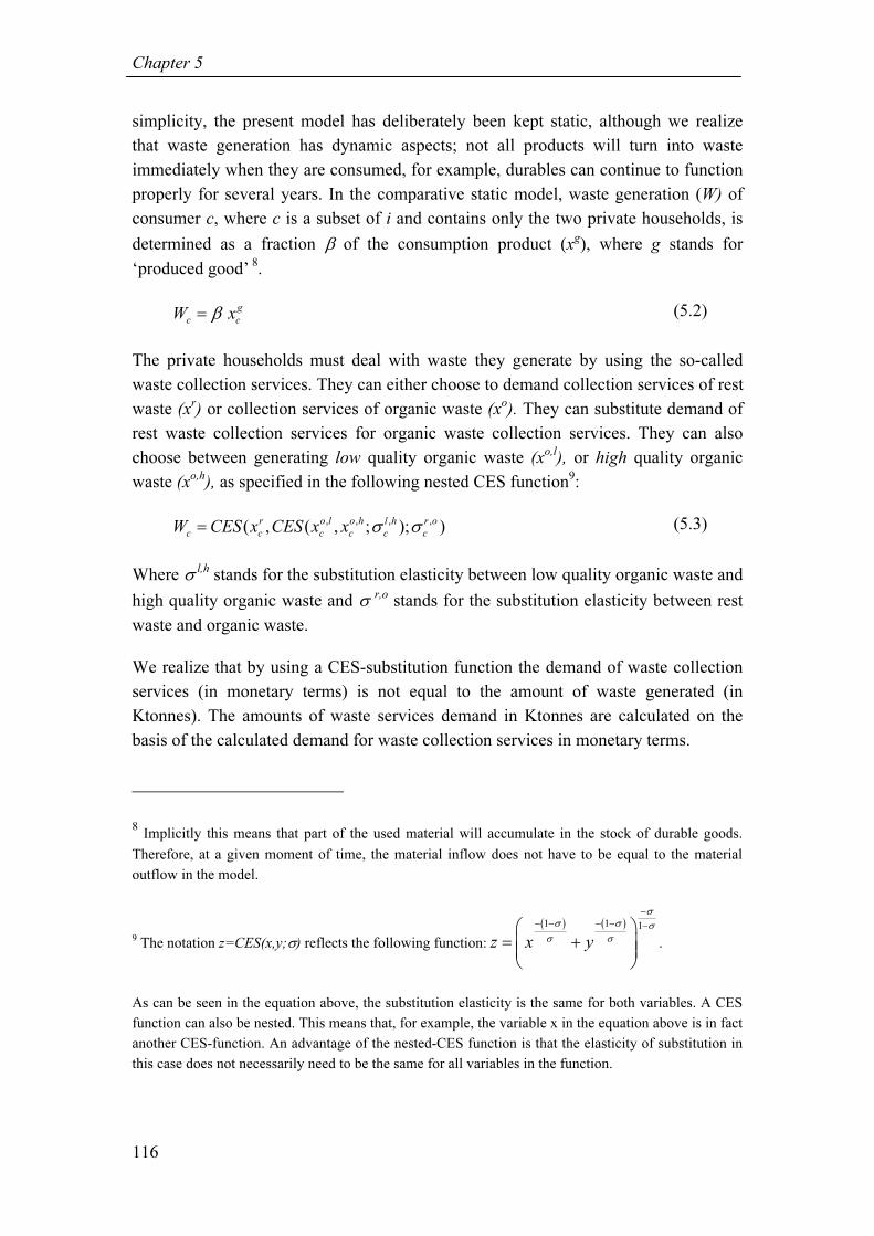
Chapter 5
116
simplicity, the present model has deliberately been kept static, although we realize
that waste generation has dynamic aspects; not all products will turn into waste
immediately when they are consumed, for example, durables can continue to function
properly for several years. In the comparative static model, waste generation (W) of
consumer c, where c is a subset of i and contains only the two private households, is
determined as a fraction β of the consumption product (xg), where g stands for
‘produced good’ 8
.
g
c cW xβ= (5.2)
The private households must deal with waste they generate by using the so-called
waste collection services. They can either choose to demand collection services of rest
waste (xr) or collection services of organic waste (xo). They can substitute demand of
rest waste collection services for organic waste collection services. They can also
choose between generating low quality organic waste (xo,l), or high quality organic
waste (xo,h), as specified in the following nested CES function9:
, , , ,( , ( , ; ); )r o l o h l h r o
c c c c c cW CES x CES x x σ σ= (5.3)
Where σ l,h
stands for the substitution elasticity between low quality organic waste and
high quality organic waste and σ r,o stands for the substitution elasticity between rest
waste and organic waste.
We realize that by using a CES-substitution function the demand of waste collection
services (in monetary terms) is not equal to the amount of waste generated (in
Ktonnes). The amounts of waste services demand in Ktonnes are calculated on the
basis of the calculated demand for waste collection services in monetary terms.
8 Implicitly this means that part of the used material will accumulate in the stock of durable goods.
Therefore, at a given moment of time, the material inflow does not have to be equal to the material
outflow in the model.
9 The notation z=CES(x,y;σ) reflects the following function:
( ) ( )1 1 1
z x y
σ
σ σ σ
σ σ
−
− − − −−
= +
.
As can be seen in the equation above, the substitution elasticity is the same for both variables. A CES
function can also be nested. This means that, for example, the variable x in the equation above is in fact
another CES-function. An advantage of the nested-CES function is that the elasticity of substitution in
this case does not necessarily need to be the same for all variables in the function.

Economic incentives and the quality of municipal solid waste
117
If private households decide to generate organic waste, they will expend labor (lw) in
separating organic waste from rest waste. Producing high quality organic waste costs
more labor than producing low quality organic waste.
The ‘production possibility set’ for the households for generating organic waste of
quality f (xc f) is given as (f= low, high):
,
o f f f
c cx lwµ≤ (5.4)
Where µ f reflects the labor costs necessary to produce a unit of organic waste of
quality f.
The three firms that are included in the model, i.e. producer of the consumption good
and the producers of the two types of collection services, produce output q of good j
under conditions of constant returns to scale, using as inputs capital (k) and labor (l).
For the sake of simplicity, we abstracted from the use of intermediate goods. The
CES-production function for these firms is:
,( , ; )k l
j j j jq CES k l σ= (5.5)
Where σk,l
is the substitution elasticity between capital and labor.
Perfect competition for each producer in the model is implicitly assumed. This
assumption, although restrictive, does not pose a problem in this model. Since the
sector ‘produced good’ is an aggregated sector representing the all production sectors
in the economy, it is natural to assume perfect competition for this sector. The
municipalities, as collectors of waste, have no competitors. Households would have to
move to be able to offer their waste to another collector. Municipalities, however, do
not strive for profit on collection. Preferably, they charge households a price exactly
equal to the marginal collection costs, just like the perfect competition assumption.
Consumers supply capital and labor to the firms. The capital supply (K), is
exogenously determined. The labor supply (L) of consumer c, however, is calculated
as the exogenous labor endowment ( L ) minus the total amount of labor used for
generating both types of organic waste (lwf):
f
c c c
f
L L lw= −∑ (5.6)
Finally, the model is closed by several balance equation, which essentially state that
the demand for any commodity, good, services, or production factor cannot exceed
the supply of that commodity.

Chapter 5
118
5.3 A numerical example
The model presented above is applied in a stylized example with numerical data from
the Netherlands. The goal of this section is to demonstrate how the main mechanisms
of the model operate and how these mechanisms are influenced by the assumptions
inherent in the model. The economic data used in the numerical example are based on
the Netherlands in the year 2000 (Statistics Netherlands, 2002b) and supplemented
with data on waste collection (collection, fee and subsidy) derived from WCM
(2000a, 2001, 2003d). To keep the model as simple as possible, we have chosen to
give the government an income dependent on capital endowments instead of an
income from taxes on labor and consumer goods10
. This has been adjusted in the
social accounting matrix.
5.3.1 Benchmark data
The accounting matrix displayed in Table 5-1 describes the initial equilibrium. The
supplies of commodities, i.e. producers’ output and consumer endowments, have
positive values; demands of commodities, i.e. production inputs and consumption,
have negative values11
.
In the benchmark data, private households pay a flat fee for the collection of both rest
waste and organic waste. This fee covers about 95% of the actual cost of waste
collection. Although the fee (and the cost-coverage rate) varies between different
municipalities in the Netherlands, the average cost-coverage rate is around 95%
(WCM, 2002).
Prices are normalized to unity according to the Harberger convention except for the
prices for waste collection of rest waste and organic waste12
. The demand for waste
collection is here displayed in thousand tonnes instead of expenditures. The prices of
10 Although less realistic, we feel that it is justified to make this assumption since our current focus is
on waste generation by private households. As we are interested in finding a first-best equilibrium
solution, we abstract from the existence of distortionary taxes in the same fashion as in Chapter 4.
11 The entries in the column times the corresponding prices add up to zero to ensure that the zero profit
condition holds: value of inputs equals value of outputs. The entries in the column of each consumer
times the corresponding price adds up to zero to ensure that the budget constraint holds: each consumer
spends exactly its income on the consumption of goods and services. The entries in each row times the
corresponding prices adds up to zero to ensure that each market clears: total demand for each
commodity must equal total supply.
12 As in Chapter 4, we adopted the Harberger convention for all unknown prices. The Harberger
convention consists of normalizing prices to unity. Thus quantities in the benchmark data represent
expenditures, or how much of a good or factor one can buy for €1.

Economic incentives and the quality of municipal solid waste
119
waste collection as shown in Table 5-1 are the average costs in million Euros of
collecting a thousand tonnes of waste (WCM, 2002).
Table 5-1 Benchmark accounting matrix for the year 2000 (expenditures in million
Euro and waste collection in thousand tonnes)
Good CS
rest
CS
organic
Traditional
consumer
Green
consumer
Gov Colsum Price
Good 759645 0 0 -358932 -172819 -227894 0 1
CS rest 0 3935 0 -3094 -841 0 0 0.269
CS organic 0 0 1457 -546 -911 0 0 0.269
Capital -554112 -424 -157 220541 106186 227966 0 1
Labor -205533 -636 -235 139323 67081 0 0 1
Fee 0 0 0 -932 -449 1380.0 0 1
Subsidy 0 0 0 980 472 -1452.0 0 1
Rowsum 0 0 0 0 0 0 0
Note: ‘Good’ stands for the consumption good; ‘CS rest’ stands for collection services of
rest waste, ‘CS organic’ indicates collection services of organic waste; ‘Fee’ is the
flat fee consumers pay to the government for collection of waste, ‘Subsidy’ stands for
the total amount of money the government gives for collection of waste as a subsidy
to the consumers. The price column gives the prices of all commodities; Rowsum is
sum of the entries in a column times the corresponding price, Colsum is the sum of
the entries of a row times the corresponding price.
As explained in Section 5.2, two types of consumers are distinguished: a ‘traditional’
consumer and a ‘green’ consumer. Based on the MOSAIC system described in Beker
(2002), the private households in the Netherlands have been divided into two
consumer types13
. According to our definition, consumers in the Netherlands may be
divided into 32.5% ‘green’ consumers and 67.5% ‘traditional’ consumers.
Private households can generate three types of waste: rest waste, low quality organic
waste and high quality organic waste. To generate organic waste, either high or low
quality, consumers have to incur costs. They can generate rest waste for free. In this
thesis, low quality organic waste and high quality organic waste are defined as
follows: 1) high quality organic waste is organic waste without any pollution and thus
100% pure. We presume that low quality organic waste is somewhat polluted by
organic waste and only 70% pure. Composting high quality organic waste will not
13 The MOSAIC system divides consumers in the Netherlands into 10 groups and 41 types based on
information about the neighborhood they live in and information about demographic, socio-economic
and life-style factors. Based on information about the influence of social factors on the amount of waste
generated (Sterner and Bartelings, 1999), these 10 groups were further aggregated into two types of
consumers.

Chapter 5
120
result in any residue, whereas composting of 100 tonnes of low quality organic waste
will result in 30 tonnes of residue that has to be incinerated.
According to information obtained from both the Waste Management Council and the
Ministry of Spatial Planning, Housing and the Environment, no recent research has
been done to determine the overall quality of organic waste collected by
municipalities. Composting units check the quality of organic waste beforehand and
decide whether the waste delivered by the municipality can be composted or not.
Their records, however, have not been released to the public. Therefore, it was
impossible to determine just how much high and low quality organic waste is actually
generated in the benchmark case. As an indication of the quality of organic waste, we
used the amount of residue that is produced during the composting process. On
average, composting of 100 tonnes of organic waste of a mixed quality results in 7
tonnes of rest waste (Beker, 2002). Given that composting of high quality organic
waste results in no residue and that composting of low quality organic waste results in
30% residue, we can calculate that the overall mixture of organic waste consists of
23.3% low quality organic waste and 76.7% high quality organic waste.
According to the way in which ‘traditional’ and ‘green’ consumers are defined, we
presume that ‘traditional’ consumers generate more low quality organic waste than
‘green’ consumers. Given that the overall composition of the waste stream consists of
23.3 percent low quality organic waste and 76.6 percent high quality organic waste
and given that the households can be divided into 32.5% ‘green’ consumers and
67.5% ‘traditional’ consumers, the percentage of low and high quality waste
generated by each consumer can be determined. Based on overall quality of the
organic waste stream and the percentage of ‘green’ consumers and ‘traditional’
consumers, it can be calculated that in the benchmark case, the ‘green’ consumer
generates 90% high quality organic waste and 10% low quality organic waste. The
‘traditional’ consumer generates 70% high quality organic waste and 30% low quality
organic waste. The amounts of low and high quality organic waste generated by the
two types of consumers are shown in Table 5-2.
The calculations on the quantity of labor necessary to generate organic waste are
based on the estimation of social costs of waste handling as found in Bruvoll (1998).
Bruvoll estimated the social costs of waste handling at 145 dollar per tonne of waste.
The amount of time spent on waste handling per week was estimated at 30 minutes a
week. This is comparable to other empirical studies like Sterner and Bartelings (1998)
and Radetzki (2000)14
. About 54% of all recyclable and organic waste collected
consists of organic waste (WMC, 2003c). If one supposes that the costs are directly
14 See Chapter 2 for more information.

Economic incentives and the quality of municipal solid waste
121
related to the amount of waste collected, the average costs of handling organic waste
are equal to 78 dollars per tonne. We may thus expect that generation of low quality
organic waste is less costly than generation of high quality organic waste, however the
generation of both high and low quality organic waste will involve many of the same
costs. For example, both high and low quality organic waste must be separated from
rest waste and the organic waste bin will, in both cases, have to be cleaned. Therefore,
we expect that generating high quality organic waste will be 10% more expensive
than the average costs and generating low quality organic waste will be 10% less
expensive than average costs. The actual labor costs in the benchmark case are
presented in Table 5-2.
Table 5-2 Additional data about the generation of organic waste in the benchmark
Traditional
consumer
Green
consumer
Low quality organic waste generated (thousand tonnes) 163.8 91.1
High quality organic waste generated (thousand tonnes) 382.2 820.0
Share of low quality organic waste in total amount organic waste 30% 10%
Units of labor necessary to generate 1 thousand tonnes of low
quality organic waste
0.072 0.072
Units of labor necessary to generate 1 thousand tonnes of high
quality organic waste
0.085 0.085
Total labor units spent on composting 44.3 76.1
Substitution elasticities for the different production sectors and the substitution
possibilities between different types of waste are given in Table 5-3. The production
sectors use capital and labor as inputs for production. They can substitute between the
use of capital and labor. Based on Draper and Manders (1996), we choose a
substitution elasticity of 0.8.
Differences in ‘environmental’ preferences are captured in the substitution elasticities
between rest waste and organic waste and between high and low quality organic
waste. The actual substitution elasticities used in the model are provided in Table 5-3.
Table 5-3 Substitution elasticities for production factors and waste categories
Good CS
rest
CS
organic
Traditional
consumer
Green
consumer
Substitution elasticity between capital and
labor (σ k,,l
)
0.8 0.8 0.8
Substitution elasticity between organic waste
and rest waste (σ r,o
)
0.6 0.3
Substitution elasticity between low and high
quality organic waste (σ l,h
)
0.9 0.1
Note: ‘Good’ stands for the consumption good; ‘CS rest’ stands for the collection of rest
waste and ‘CS organic’ stands for the collection of organic waste.

Chapter 5
122
Consumers have the option of substituting rest waste for organic waste and low
quality organic waste for high quality organic waste. On average, the stream of rest
waste contains about 32% of organic waste. Substituting rest waste for organic waste
does not mean that consumers make organic waste from, for example, a tin can by
using labor as an input, but that they either separate organic waste from rest waste, i.e.
throwing vegetable waste in the organic waste bin instead of in the rest waste bin, or
that they throw rest waste in the organic waste bin and thus pollute the organic waste
stream. To ensure that households do not generate high quality organic waste out of
thin air, upper values on the extra amounts of high quality organic waste that can be
generated have been set, based on the average amount of organic waste in the stream
of rest waste.
Several studies have estimated the own price elasticity of the generation of rest waste.
In this chapter, the substitution elasticities between rest waste and high and low
quality organic waste have been based on the price elasticity estimated by Fullerton
and Kinnaman (1996). They established an own price elasticity of –0.058. Other
estimates of price elasticities can be found in Hong et al. (1993), Wertz (1976),
Jenkins (1993) and Linderhof et al. (2001) (see Chapter 2 for more information)15
.
Since no information is available about the quality of organic waste, it is difficult to
calibrate the substitution elasticity between low and high quality organic waste. Based
on our expert opinion we assert that the demand is inelastic and thus the substitution
elasticity is smaller than unity. By definition, the substitution elasticity will be larger
for the ‘traditional’ consumer than for the ‘green’ consumer.
5.3.2 Results
The model, as specified in Section 5.2, is used to calculate the effects of the
introduction of a unit-based pricing scheme for the collection of rest waste. This
means that private households will have to pay the equilibrium price, which equals the
marginal costs of producing this service, for the collection of rest waste. Private
households will still pay a flat fee for the collection of organic waste.
Comparing the benchmark situation, which includes the flat fee-pricing scheme for
waste collection, to the unit-based price scenario, which includes the unit-based
pricing scheme for waste collection gives an indication of the expected results of
introducing such a policy change. In Table 5-4, the changes in the main variables are
presented.
15 The own-price elasticity (ε) of good i is equal to: ( 1)ieε σ σ= − + − , where σ is the substitution
elasticity and ei is the proportion of expenses for good i.

Economic incentives and the quality of municipal solid waste
123
Table 5-4 Results for the main variables in the ‘flat fee scenario’ and ‘unit-based price
scenario’ (expenditure in million Euro and waste collection in Ktonnes) and the
percentage change as compared to the benchmark case
Flat fee Unit-based fee
Traditional
consumer
Green
consumer
Traditional consumer Green consumer
Consumption good 358932 172819 358903 (-0.01%) 172813 (0.00%)
Collection rest waste 3093.66 841.34 2832.32 (-8.45%) 726.11 (-13.70%)
Collection organic waste 545.94 911.06 806.99 (47.82%) 1026.23 (12.64%)
As shown in Table 5-4, introducing a unit based pricing scheme for collection of rest
waste has a significant effect on the demand for collection of both rest and organic
waste. These results are as expected: since organic waste may be collected free of
charge, households will start to substitute the more expensive rest waste with organic
waste. This holds especially for the ‘traditional’ consumer who has a large
substitution elasticity between rest waste and organic waste. The introduction of a
unit-based price, however, also has the undesirable effect of increasing the quantity of
low quality organic waste (Table 5-5).
Table 5-5 Results for organic waste categories for the ‘flat fee’ scenario and ‘unit-
based price’ scenario in Ktonnes (in brackets % change as compared to flat fee)
Flat fee Unit-based fee
Traditional
consumer
Green
consumer
Traditional consumer Green consumer
Low quality organic waste 163.78 91.11 267.57 (63.37%) 104.08 (14.24%)
High quality organic waste 382.16 819.95 539.41 (41.15%) 922.15 (12.46%)
Share of low quality
organic waste
30.00 10.00 33.16 (10.53%) 10.14 (1.40%)
Private households start to produce more low quality organic waste instead of high
quality organic waste (see Table 5-5). Substitution of rest waste for low quality
organic waste is especially evident among ‘traditional’ consumers. ‘Green’
consumers, who have more concern for the environment, increase both their
production of low quality organic waste and their production of high quality organic
waste.
Since both types of organic waste are collected together, the share of low quality
organic waste will greatly affect the overall quality. If the amount of low quality
organic waste is relatively large compared to the amount of high quality organic
waste, then the overall quality of the organic waste will be low. If unit-based pricing
is introduced, on average about 6.7% of organic waste collected will consist of rest

Chapter 5
124
waste. In the flat fee pricing system, only 5.5% of organic waste consists of rest
waste.
The ‘green’ consumer does not pollute the organic waste stream as much as the
‘traditional’ consumer. The percentage of rest waste thrown away with organic waste
is about 3.1%. This percentage is constant for both the flat fee pricing system and the
unit-based pricing system. ‘Traditional’ consumers contribute more rest waste to the
organic waste stream. The percentage of rest waste thrown away with organic waste
increases from 9.8% to 11%. IPH (1995) shows that composting units generally will
not accept such low quality organic waste as generated by the ‘traditional’ consumers.
This means that the composting unit will reject waste, which is collected in districts
with relatively many ‘traditional’ consumers. Waste in this case must either be
incinerated or landfilled, which increases waste treatment costs. Since actual
composting is not included in this model, it is impossible to predict how much the
waste treatment costs will increase due to waste leakage. In Chapter 6, an analysis of
these costs is made.
The total amount of waste generation is not affected by the policy change. As
prevention is not included in the model, consumers can only reduce total generation of
waste by consuming less. As the income of the consumers is only minimally affected
by the policy change, the consumers will not reduce consumption and thus total waste
generation remains constant. Table 5-5 illustrates that the share of low quality organic
waste has increased. The overall share of low quality in the total organic waste stream
has risen from 17% to 20%. The unit-based pricing scheme leads to waste leakage and
may therefore not be suitable to provide the correct incentives to private households to
minimize waste generation.
5.3.3 Sensitivity analysis
This section deals with the sensitivity of the model. The results as presented in the
Section 3.3.2 depend largely on the parameters used. Three parameters in particular
are difficult to measure or estimate and therefore require careful examination. These
are: (i) the substitution elasticity between rest waste and organic waste; (ii) the
substitution elasticity between low quality organic waste and high quality organic
waste; (iii) the labor cost of generating low and high quality organic waste.
The following procedure has been used for the sensitivity analysis. The value of the
parameter is changed in a number of (equidistant) steps from the lower to the upper
value of the range of the sensitivity analysis. The effects of these parameter changes
are calculated for all variables of the model. The impact of the variables, rest waste,
low quality organic waste and high quality organic waste, are presented below.

Economic incentives and the quality of municipal solid waste
125
Substitution elasticity between rest waste and organic waste
As empirical studies report several different values for the price elasticity of rest
waste (see Chapter 2), in this study a sensitivity analysis was performed for the
substitution elasticity between rest waste and organic waste. This substitution
elasticity is lower for the ‘green’ consumers than for the ‘traditional’ consumers. We
have chosen to keep the ratio of the substitution elasticities between both consumers
constant. Figure 5-2 shows the results of the sensitivity analysis. All other parameters
are kept constant at benchmark levels.
0
500
1000
1500
2000
2500
3000
3500
4000
0.5 0.6 0.7 0.8 0.9 1.0 1.1 1.2 1.3 1.4 1.5 1.6 1.7 1.8 1.9 2.0 2.1 2.2
Index for sub. elas. between rest waste and organic
waste (benchmark=1)
Was
te (
thousa
nd t
onnes
)
Rest waste
High qualityorganic waste
Low qualityorganic waste
Figure 5-2 Sensitivity analysis for the substitution elasticity between rest waste and
organic waste: impacts on quantities of waste
Note: The substitution elasticity is calculated as the benchmark substitution elasticity (0.6
and 0.3 respectively) multiplied by a factor δ. The value of factor δ is shown on the x-
axis.
The substitution elasticity between rest waste and organic waste determines how
much rest waste is generated. If the substitution elasticity is quite high then only 2900
thousand tonnes of rest waste will be generated. If, however, the elasticity is quite low
the amount of rest waste increases to about 3750 thousand tonnes. Note that both the
amounts of low quality organic waste and high quality organic waste grow as the
substitution elasticity increases, which means that consumers are both separating more
waste and discarding part of their rest waste into the organic waste bin.
Substitution elasticity between low quality and high quality organic waste
The second parameter that is examined is the substitution elasticity between low
quality and high quality organic waste. As there is no data on how to calculate the
value of this parameter, it is essential that a sensitivity analysis for this parameter is

Chapter 5
126
done. This substitution elasticity differs between the two consumers and the ratio
between these two elasticities has been kept constant. The results of this sensitivity
analysis are shown in Figure 5-3.
250
750
1250
1750
2250
2750
3250
0.6 0.8 1.0 1.2 1.4 1.6 1.8 2.0 2.2 2.4
Index for sub. elas. high low quality organic waste
(benchmark=1)
Was
te (
thousa
nd t
onnes
)
.
Rest waste
High quality
organic waste
Low quality
organic waste
Figure 5-3 Sensitivity analysis for the substitution elasticity between low and high
quality organic waste: impacts on quantities of waste
Note: The substitution elasticity is calculated as the benchmark substitution elasticity (0.9
and 0.1 respectively) multiplied by a factor δ. The value of factor δ is shown on the x-
axis.
The amount of waste generated is barely sensitive to the substitution elasticity
between low and high quality organic waste. When this substitution elasticity
increases, a little more low quality organic waste is generated and marginally less
high quality organic waste. The amount of rest waste generated is not affected at all.
Obviously it is mostly the substitution elasticity between rest waste and organic waste
that determines how much rest waste is transformed in high and low quality organic
waste.
Labor cost organic waste
Another parameter that can affect the efficiency of the policy change is the actual
labor cost of producing low quality and high quality organic waste. In the benchmark
case, it is assumed that 0.072 units of labor are necessary to produce one unit of high
quality waste (units in million tonnes) and 0.085 units of labor to produce one unit of
low quality organic waste. This means that the labor costs parameter has a value of
13.89 for low quality organic waste and a value of 11.76 for high quality organic
waste. The higher the labor costs parameter, the lower the actual labor costs. In this
sensitivity analysis, the labor costs are varied from 56 percent to 333 percent of the
benchmark level, this means that the value of the labor costs parameters are varied
from –150% to 190%. The proportional difference between costs of generating low

Economic incentives and the quality of municipal solid waste
127
and high quality organic waste, however, is maintained. The results are presented in
Figure 5-4.
0
500
1000
1500
2000
2500
3000
3500
4000
4500
0.4 0.5 0.6 0.7 0.8 0.9 1.0 1.1 1.2 1.3 1.4 1.5 1.6 1.7 1.8 1.9
Index for labor cost parameter (benchmark =1)
Was
te (
tho
usa
nd
to
nn
es)
Rest waste
Low quality
organic waste
High quality
organic waste
Figure 5-4 Sensitivity analysis labor cost organic waste: impacts on quantities of
waste
Note: The labor cost parameter is calculated as the benchmark labor cost parameter (13.89
and 11.76 respectively) multiplied by a factor δ. The value of factor δ is shown on the
x-axis.
As expected, the lower the labor costs, the higher the organic waste generation, and
thus the lower the amount of rest waste generated. It is remarkable that the rate of
substitution between rest waste and organic waste changes when the labor costs
become higher. If the labor costs are high, a small change will result in a far larger
change in the substitution rate than if the labor costs are low.
Interaction between labor costs of composting and substitution elasticity between rest
waste and organic waste
Finally, the interaction between the labor cost of generating organic waste and the
substitution elasticity between rest waste and organic waste was examined. In Figure
5-5, the impact on the generation of rest waste is shown. The quantity of rest waste
that is generated is greatly affected by the substitution elasticity between rest waste
and organic waste. The higher the substitution elasticity, a lesser the amount of rest
waste is generated. The labor costs greatly affect the production of rest waste, but
only if the substitution elasticity between rest waste and organic waste is fairly large.
For small elasticity levels, the amount of rest waste is hardly affected. The higher the
elasticity, the greater the impact of labor costs.

Chapter 5
128
0.61.0
1.41.8
2.2
0.6
1.0
1.4
1.8
2.2
200
700
1200
1700
2200
2700
3200
3700
4200
Rest waste
(thousand tonnes)
Index for sub. elas. rest and
organic waste (benchmark=1)
Index for labor
cost parameter
(benchmark=1)
Figure 5-5 Interaction between labor cost and substitution elasticity between rest
waste and organic waste: impacts on quantity of rest waste
Figure 5-6 shows the quantity of low quality organic waste generated. The effects are
even more profound for the generation of low quality organic waste.
0.6 0.8 1.0 1.2 1.4 1.6 1.8 2.0 2.2 2.4
0.6
1
1.4
1.8
2.2
200
300
400
500
600
700
800
900
Low quality
organic waste
(thousand tonnes)
Index for sub. elas. rest and organic
waste (benchmark=1)
Index for labor
cost parameter
(benchmark=1)
Figure 5-6 Interaction between labor cost and substitution elasticity between rest and
organic waste: impacts on quantity of low quality organic waste
If we introduce higher labor costs in combination with small substitution elasticity
levels, the amount of low quality organic waste generated increases by about 30%
when a unit-based price is implemented. If we introduce higher labor costs combined

Economic incentives and the quality of municipal solid waste
129
with a large substitution elasticity, the amount of low quality organic waste increases
by nearly 250%.
5.4 Discussion and conclusions
In this chapter, the effects of introducing a unit-based pricing scheme for the
collection of rest waste have been analyzed. A general equilibrium model in the
Negishi format was presented, with the possibility of generating three types of waste.
In the model the consumers were given the possibility of substitution for these
different types of waste, i.e. high quality organic waste, low quality organic waste and
rest waste. With this model it is possible to illustrate some important aspects of the
waste sector and the dangers of waste leakage. Waste leakage occurs when
households throw rest waste into the organic waste or recyclable waste stream, thus
polluting the organic and recyclable waste stream and making recycling or
composting of this waste streams more expensive or impossible.
The results demonstrate that introducing a unit-based pricing scheme may lead to
significant waste leakage. Waste leakage will greatly influence the effectiveness of
the policy change. The ‘traditional’ consumers, who have less preference for a clean
environment, are given strong incentives to discard part of their rest waste in the
organic waste stream, thereby creating low quality organic waste, which will be more
difficult to compost.
The sensitivity analysis shows that these results are quite sensitive to several
parameters in the model. The labor cost of separating organic waste will especially
influence how much rest waste is substituted by low quality organic waste. The
substitution elasticity between organic waste and rest waste also influences the
effectiveness of the policy. The substitution elasticities between low and high quality
organic waste hardly have an effect on the optimal solution of the model.
This chapter only investigated how much waste leakage would occur when unit-based
pricing was introduced. It did not explore how the composting costs would be
affected. Therefore, it is difficult to say how the benefits of having less rest waste
compare to extra composting costs due to lower quality of waste. In future research,
the waste treatment sector should be included in the model in greater detail.
Furthermore, it would be interesting to empirically determine several parameters
concerning organic waste, such as the elasticity between low and high quality waste
and the amount of low and high quality waste generated.
Waste leakage occurs when a unit-based price is introduced for the collection of rest
waste. How much waste leakage occurs depends to a large extent on the type of
consumers living in the municipality. Especially larger municipalities or mega-cities

Chapter 5
130
with a relatively large share of ‘traditional’, consumers can expect problems
concerning waste leakage. As waste leakage leads to a decline in the quality of
organic waste, potentially resulting in the situation where organic waste can no longer
be composted but instead must be landfilled or incinerated, unit-based pricing will be
less environmentally beneficial than might be expected. The results show that
‘traditional’ consumers pollute the organic waste stream to such as extent that it can
no longer be composted. Since waste is collected in relatively small quantities, about
28 tonnes per garbage truck, it can be expected that districts with a higher percentage
of ‘traditional’ consumers will generate organic waste that cannot be composted. It is
therefore advisable for unit-based pricing to only be introduced in municipalities that
have a large share of ‘green consumers’. It is expected that substantial waste leakage
will occur, particularly in the larger municipalities, since these municipalities have
many districts with considerably more ‘traditional’ consumers.
As a unit-based pricing scheme is very efficient for lowering the amount of rest waste
generated, it seems desirable that technologies, which enable us to separate rest waste
from organic waste and produce high quality compost of cleaned organic waste, be
invested in. Although it is already possible to mechanically separate recyclable and
organic waste from rest waste (see Oorthuys and Brinkmann, 2000), the application of
this technique is still in an experimental phase. It would be advisable for more to be
invested in the development of such technologies. Only if this technology were
available at low costs, would the implementation of unit-based pricing on a larger
scale be recommended.

Economic incentives and the quality of municipal solid waste
131
Appendix 5-A Specification of relevant equations
5-A.1 Model specification for a fixed fee for the collection of organic and rest waste
Welfare
Total welfare function:
ln( ) r r c o
i i
i
TWF u TD TDα ξ ξ= + +∑ (A.1)
Where utility of consumers depends on the consumption of the consumer goods 16
g
i iu x≤ For i = 1....3 (A.2)
In the benchmark case consumers have no price incentive to generate organic waste. As data
for the Netherlands show that organic waste is generated even if municipalities charge a flat
fee, organic waste generation has been included in the benchmark case. To ensure that organic
waste is generated in the benchmark case, two extra consumers are introduced, who only
derive benefits from the generation of organic waste. This modeling trick can be seen as if a
consumer derives utility from generating organic waste due to the fact that the consumer is
doing something beneficial for the environment.
, , ,( , ; )o l o h l h
i i iu CES x x σ≤ for i = 4,5 (A.3)
Production function goods and collection services
( , ; )j j j j
klq CES k l σ= for each j (A.4)
16 As mentioned in Section 5.2, to include the subsidy-cum-tax scheme in the model the total cost of the
per unit subsidy (ξ) on waste collection of both rest waste (ξ r TD r ) and organic waste (ξ o TD o) has to
be added to the total welfare function due to technical reasons. This is done solely to change the
marginal prices of waste collection. See Chapter 4 for more information on this subject.

Chapter 5
132
Market clearance
Goods market balance:
g g g
i
i
x q p≤ ⊥∑ (A.5)
By taking the marginal value of the balance constraint, the price vector p can be determined
(this is symbolized by ⊥ p). The price vector is used in calculating the budget constraint and
in determining the Negishi weights.
Capital market balance
j k
i
j i
k K p≤ ⊥∑ ∑ (A.6)
Labor market balance:
j l
i
j i
l L p≤ ⊥∑ ∑ (A.7)
Where labor supply is determined by:
f
i i i
f
L L lw= −∑ for i = 1....3 (A.8)
Collection rest waste market balance:
r r r
i sub
i
x TD p≤ ⊥∑ (A.9)
r r r
TD q p≤ ⊥ (A.10)
Collection organic waste market balance:
, ,
o l o h o o
i i sub
i i
x x TD p+ ≤ ⊥∑ ∑ (A.11)
o o o
TD q p≤ ⊥ (A.12)
Waste equations
Waste generation as percentage consumption:
g
c cW xβ= (A.13)

Economic incentives and the quality of municipal solid waste
133
, , , ,( , ( , ; ); )r o l o h l h r o
i i i i i iW CES x CES x x σ σ= (A.14)
,
o f f f
c cx lwµ≤ (A.15)
Calculation Negishi weights
Budget constraint consumer i:
k l g g r r o o
i i i i i sub i sub ip K p L F LST p x p x p x+ − − = + + for i=1,2 (A.16)
Budget constraint government:
k g g
i i i i
i
p K F T LST p x+ − + =∑ for i=3 (A.17)
Total expenditure government is kept constant at benchmark level. If for any reason
expenditure would change, then the income of the government is compensated through lump
sum transfers. Where:
( )o k
gov i i
i
LST Y p K F T= − + −∑ for i = 3 (A.18)
Total cost subsidy calculated as a lump sum transfer:
,r r o o f
i i
i i f
T x xξ ξ= +∑ ∑∑ (A.19)
5-A.2 Model specification including a unit-based pricing scheme for the collection of rest
waste
In the unit-based pricing scheme model the following equation are changed:
Total welfare function (replaces equation A.1):
ln( ) o o
i i
i
TW u TDα ξ= +∑ (A.20)
Market balance constraint for collection rest waste (replaces equations A.9 and A.10) :
r r r
ix q p≤ ⊥∑ (A.21)
Budget constraint consumer I (replaces equation A.16):

Chapter 5
134
k l g g r r o c
i i i i i i sub ip K p L F LST p x p x p x+ − − = + + for i = 1,2 (A.22)
Where fee refers to the fee for collection of organic waste only.
Budget constraint government (replaces equation A.17):
k g g
i i i i
i i
p K F T LST p x+ − + =∑ ∑ for i = 3 (A.23)
Total cost subsidy on collection of organic waste calculated as a lump sum transfer (replaces
equation A.19):
,cc c f
i
i f
T xξ= ∑∑ (A.24)
Appendix 5-B Definition of indices, parameters, and variables
Indices
Label Range Description
c 1…2 traditional and green consumer
f 1...2 quality organic waste (low, high)
i 1...5 Consumers
j 1...3 goods (consumer good g, collection service rest waste r, collection
service compost waste c)
sub 1 Subsidy
z 1...5 commodities (goods, capital and labor)
Parameters in GAMS specification
Symbol Description
α Negishi weight
β waste percentage
µ labor cost for generating organic waste

Economic incentives and the quality of municipal solid waste
135
σk,l substitution elasticity between labor and capital
σl,h substitution elasticity between low and high quality organic waste
σ r,o substitution elasticity between rest waste and organic waste
ξ subsidy wedge
F flat fee for waste collection
K endowment of capital
L endowment of labor
LST lump sum transfer to keep income of government constant
p Price
Pc Price including subsidy
T Total costs subsidy waste collection
Y0 initial income
Variables in GAMS specification
Symbol Description
k capital use
l Labor use
lw Labor used for generation of organic waste
q production
TD Total demand for waste collection services
TW Total welfare
u utility
W Total generation of waste
x consumption

Chapter 5
136

137
6. Modeling economies of scale, transport costs and the
location of waste treatment units in a general equilibrium
framework
6.1 Introduction
The waste market is rapidly changing. In the Netherlands, one can observe a trend
towards an increasing scale, concentration, and vertical integration, alongside a
movement towards a multi-utility structure (WMC, 2002). The increasing scale of
waste treatment units has diminished the influence of municipalities in the
management of these companies. Where waste treatment was once mostly a municipal
affair, it has become far more privatized. Energy companies have also become
interested in merging with waste treatment units thus creating multi-utility companies.
Waste treatment companies are interested in vertical integration; several of the largest
companies are currently focusing on providing all services connected to waste
treatment, from collection to final disposal. Moreover, international companies have
become interested in providing their services throughout the whole of Europe (WMC,
2002).
Until 2000, Dutch laws prohibited the transportation of waste over provincial
boundaries. Since January 2000, these laws have been revoked, which means that
municipalities and companies are now allowed to transport waste outside the
boundaries of their province and offer it to any waste treatment unit in the
Netherlands. This means that more competition has been introduced into the waste
market. Furthermore, the boundaries between countries in the European union have
ceased to exist for transport of recyclable waste and are expected to disappear for
combustible waste, which may also ultimately result in a reorganization of the waste
market.
All of these developments have had important consequences for the waste
management problem. Not only should the quantity of waste generated be minimized
as cost-efficiently as possible, but it is also important that by choosing the cheapest
waste treatment unit the waste treatment costs are reduced. Larger waste treatment
units are able to treat waste against lower costs due to economies of scale (see, for
example, Oorthuys, 1995 and WMC, 2003e). Larger units could also reduce harm to
the environment at lower costs per unit of waste treatment. Naturally, this also means
that waste will, in general, be transported over longer distances thus incurring both
greater transport costs and more transport emissions.

Chapter 6
138
Thus far the spatial aspects of the waste treatment problem have been analyzed mostly
from within an optimization setting. Existing studies have focused on finding the
optimal location of a waste treatment unit in order to minimize the waste treatment
costs for society. Examples of these kinds of studies can be found in Opaluch et al.
(1993), Macauley et al. (2002) and Ye and Yezer (1997).
These studies focus on determining the optimal waste treatment method given a
certain quantity of waste. The quantity of waste generated, however, should not be
taken as a given. Waste generation will to some extend depend on how waste is
treated and how large the costs of waste treatment are. If waste treatment becomes
more expensive, industries, for example, will start to recycle more of their waste to
prevent waste disposal costs. To a lesser extent, households will also start to reduce
waste generation. Households faced with a higher disposal tax will not only try to
prevent waste generation by recycling and composting waste at home, but also by
increasing the illegal disposal of waste. In turn, the quantity of waste generated affects
the optimal choice between waste treatment options and the optimal location and size
of the waste treatment units. A small quantity of waste may be treated in a local waste
treatment unit; a larger waste stream or a waste stream of lower quality1 may have to
be sent to a larger waste treatment unit.
This chapter presents a model, which simulates the market for municipal solid waste.
In this model, several municipalities are distinguished. Waste is generated in each
municipality. This waste must be composted, incinerated, or landfilled. Depending on
the price of waste treatment, transport costs, and emission restrictions, municipalities
decide how and where to treat the waste.
Since we feel that the interaction between waste generation, the choice of waste
treatment and choice of the optimal location of waste treatment units can best be
analyzed in a general equilibrium context, we choose to build a general equilibrium
model. The possibility of modeling the interaction between several markets is the
main advantage of this type of model. Special attention will be paid to how the spatial
aspects of the waste management problem can be included in a general equilibrium
framework. The novelty in this approach is the focus on how the choice of a certain
waste treatment unit is simultaneously affected by economies of scale, transport costs,
quality of waste, emission restrictions, and policies aimed at reducing waste
generation.
1 The quality of the waste stream can be very important in determining the choice between waste
treatment options. For example, organic waste heavily polluted with rest waste will be expensive or
impossible to compost. In such a case, it may be necessary to incinerate the waste instead of
composting it (see, for example, Chapter 5).

Modeling economies of scale, transport cost and location of waste treatment units
139
This model will be applied to a stylized setting of the waste market in a region of the
Netherlands. This example will illustrate how the quality and quantity of waste
generated significantly influences the choice of waste treatment methods, their size,
and location. Furthermore, it will be demonstrated that the choice of optimal waste
treatment methods, size, and location can significantly influence the cost-
effectiveness of a policy change. A unit-based price for the collection of rest waste
will be introduced and we will show that although such a policy change reduces waste
generation, as recent studies such as Fullerton and Wu (1998) and Choe and Frasier
(1999) have demonstrated, it will also decrease the quality of organic waste, thus
increasing the composting and transport costs of waste. The model presented in this
chapter is applied to the municipal solid waste market in the Netherlands, but is
written in general terms and can easily be applied to the municipal solid waste market
in any other industrialized country.
The structure of this chapter is as follows: Section 6.2 introduces the model
specification. Section 6.3 describes the data used and presents the results of different
scenarios. Section 6.4 concludes.
6.2 Modeling the spatial aspects of the municipal solid waste
problem
6.2.1 General introduction to the model structure
The model presented in this section is an extended version of the model used in
Chapter 5. The main aspects of the model will shortly be discussed and more attention
will be paid to the new elements, namely economies of scale, transport costs, and
emission rights. The structure of the model is illustrated in Figure 6-1.
We distinguish only one producer who makes a ‘produced’ good. The private
households and the government consume the ‘produced’ good. Four municipalities
are distinguished in the model. In each municipality, two types of consumers: a
‘traditional’ consumer and a ‘green’ consumer are modeled, just as in Chapter 5. The
‘traditional’ consumer has little preference for the environment. The ‘green’ consumer
has some preference for a clean environment. Each municipality differs in the number
of consumers and the share of ‘traditional’ and ‘green’ consumers.
Consumption of the ‘produced good’ results in waste. Consumers can choose to
generate three types of waste, namely rest waste, low quality organic waste and high
quality organic waste. The private households must invest labor in the separation of
organic from rest waste. Generating high quality organic waste will cost more labor
than generating low quality organic waste.

Chapter 6
140
Municipality A
Producer
Consumption good
Municipality B
Traditional
consumer
Green
consumer
Municipality A
Traditional
consumer
Green
consumer
Municipality D
Traditional
consumer
Green
consumer
Municipality C
Traditional
consumer
Green
consumer
Incineration
Large
unit
Medium
unit
Small
unit
Landfilling
Large
unit
Medium
unit
Small
unit
Composting
Large
unit
Medium
unit
Small
unit
Organic
wasteRest waste
Emissions Emissions Emissions
Residue
Figure 6-1 Representation of the model structure
Consumers can either pay a flat fee for the collection of waste or a unit-based price.
The flat fee-pricing scheme will be implemented in the model using the subsidy-cum-
tax scheme as described in Chapter 4. To recapitulate the idea of this scheme,
consumers pay the equilibrium price for collection of waste to the municipalities.
They are reimbursed with the exact amount of money in the form of a subsidy from
the government. Thus the perceived price of collection for the consumers equals zero.
The consumers pay a direct tax to the government to reimburse the costs of the
subsidy. In such a way, the consumers do pay for waste collection, but the amount
they pay is not coupled with the quantity of waste they generate, the exact definition
of a flat fee.
The municipality, who is a producer of collection services, collects rest waste and
sends it to an incinerator or a landfill. Low quality organic waste and high quality
organic waste are both collected together and sent to a composting unit. The costs of
composting depend on the quality of the organic waste stream. If the overall quality of
organic waste is low (i.e. there is a large share of low quality organic waste in the
entire organic waste stream), it will be difficult to compost the waste. Part of the
waste will be rejected by the composting unit and sent to an incinerator. This will
greatly increase the costs of composting.
Spatial aspects in the model: transport costs and economies of scale
In the model, the spatial aspects of the waste management problem are integrated in a
general equilibrium framework. This means including transporting costs and
economies of scale. In the model, municipalities collect waste and send it to a waste
treatment unit. The municipality has the choice between sending waste to a small, a

Modeling economies of scale, transport cost and location of waste treatment units
141
medium or a large sized waste treatment unit. The small unit is located close to the
municipality; the medium and large waste treatment units are located further away.
Thus the larger waste treatment units are more efficient in waste treatment, but they
are more expensive with regard to transport costs. The key characteristics of the
spatial aspects are depicted in Figure 6-2.
According to the standard specification of general equilibrium models, we assume
perfect competition between production sectors. This implies that there is also perfect
competition between waste treatment units. In reality this may not be the case. For
example, contracts between municipalities and incinerators exist, which specify the
quantity of waste municipalities must deliver to the incinerator. It goes beyond the
scope of this thesis to include such imperfect competition in the model. However, in
future research it would be interesting to see how monopolistic behavior of waste
treatment units influence the results.
Municipality
Large WTU
Medium WTU
Small WTU
Transport
BA
C D
Figure 6-2 Spatial aspects in the model for four municipalities
Note: WTU stands for waste treatment unit
The three waste treatment units, namely the landfill unit, the incineration unit, and the
composting unit, offer waste treatment services to the municipalities. These units use
capital and labor as inputs to the production process. The composting unit, besides
using capital and labor, also uses incineration services to get rid of both the residue
and the rejected low quality organic waste.
Due to economies of scale in the production process, the larger waste treatment units
offer waste treatment services at a lower price. In the context of our study, several
locations are exogenously specified for each waste treatment unit. Given transport

Chapter 6
142
costs and waste treatment costs of each unit, municipalities will choose the least
expensive option. Except for the differentiated marginal costs, the services provided
by the different sizes of a waste treatment unit are identical.
Composting costs are also differentiated according to the quality of organic waste. To
compost organic waste of a lower quality, the waste must be cleaned. If the organic
waste is too badly polluted it cannot be composted. The composting unit will thus
have to send the waste to an incinerator. It is, therefore, more expensive to compost
organic waste of a lower quality. The costs of composting low quality organic waste
will also be differentiated according to the size of the composting unit. Smaller
composting units tend to charge a higher price to compost low quality organic waste
than larger units.
6.2.2 The model represented in equations
As stated above, the model presented in this section is an extended version of the
model presented in Chapter 5. The main differences between this model and the
model in Chapter 5 are the introduction of several municipalities, waste treatment
units, economies of scale, transport costs, and emissions generated by waste
treatment.
Welfare, production, consumption and waste generation
The model is built like a standard general equilibrium model in the Negishi format.
This means that total welfare is maximized subject to utility constraints, balance
constraints and production possibility sets. The total welfare function is shown in
equation 6.1. Total welfare (TWF) is defined as the sum of the utilities (ui) of each
consumer i. The utility of each consumer is weighted by a factor αi, the so-called
Negishi weight2. Each consumer derives utility from the consumption of the
consumption good (xIg).
ln[ ( )]g
i i i
i
TWF u xα=∑ (6.1)
2 The value of the Negishi-weights is determined in such a way that the budget constraint for each
consumer holds. This means that each consumer will spend exactly its entire income on the
consumption of goods and services or savings. See Chapter 4 for more information about the
determination of the Negishi-weights.
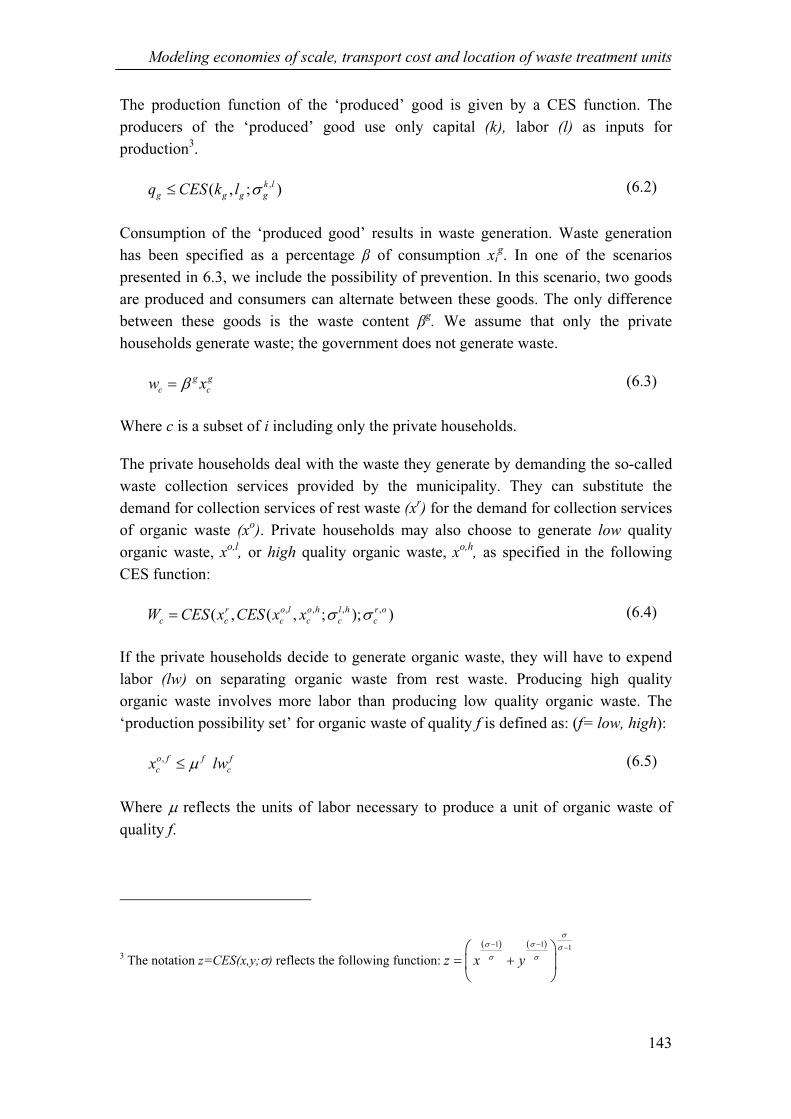
Modeling economies of scale, transport cost and location of waste treatment units
143
The production function of the ‘produced’ good is given by a CES function. The
producers of the ‘produced’ good use only capital (k), labor (l) as inputs for
production3.
,( , ; ) k l
g g g gq CES k l σ≤ (6.2)
Consumption of the ‘produced good’ results in waste generation. Waste generation
has been specified as a percentage β of consumption xig. In one of the scenarios
presented in 6.3, we include the possibility of prevention. In this scenario, two goods
are produced and consumers can alternate between these goods. The only difference
between these goods is the waste content βg. We assume that only the private
households generate waste; the government does not generate waste.
g g
c cw xβ= (6.3)
Where c is a subset of i including only the private households.
The private households deal with the waste they generate by demanding the so-called
waste collection services provided by the municipality. They can substitute the
demand for collection services of rest waste (xr) for the demand for collection services
of organic waste (xo). Private households may also choose to generate low quality
organic waste, xo,l, or high quality organic waste, xo,h, as specified in the following
CES function:
, , , ,( , ( , ; ); )r o l o h l h r o
c c c c c cW CES x CES x x σ σ= (6.4)
If the private households decide to generate organic waste, they will have to expend
labor (lw) on separating organic waste from rest waste. Producing high quality
organic waste involves more labor than producing low quality organic waste. The
‘production possibility set’ for organic waste of quality f is defined as: (f= low, high):
,
o f f f
c cx lwµ≤ (6.5)
Where µ reflects the units of labor necessary to produce a unit of organic waste of
quality f.
3 The notation z=CES(x,y;σ) reflects the following function:
( ) ( )1 11
z x y
σ
σ σσ
σ σ
− −
−
= +

Chapter 6
144
The amounts of labor expended on generating organic waste affects the labor supply.
The labor supply L of each consumer i is calculated as the exogenous labor
endowment, L , minus the total amount of labor used for generating both types of
organic waste.
f
c c c
f
L L lw= −∑ (6.6)
Transport costs
The municipality collects the waste generated by private households and sends it to a
waste treatment unit. The municipality must pay transport costs for transporting waste
to a waste treatment unit. Transport costs are modeled as if the municipality demands
transport services of a transport company. Waste treatment units will charge a price to
treat the waste. Each different waste treatment method, (index m= incineration,
landfilling, composting) will charge a different price, according to the marginal waste
treatment costs.
The production function for waste collection services is given by a nested Leontief-
CES function. It depends on the inputs of capital, labor, transport services (ts), and
waste treatment services (wts). Municipalities can choose between different waste
treatment methods, i.e. incineration, landfilling, composting, and different sizes of
waste treatment units. Each waste treatment unit comes in three different sizes: small,
medium, and large (index s = small, medium, large). The production of waste
collection services of each municipality j is given as:
, , ,min( ( , ; ), ( ; ), ) k l m s m s
cs cs cs cs cs csq CES k l CES wts tsσ σ≤ (6.7)
Municipalities cannot make a completely free choice between the three different
waste treatment options. Organic waste will have to be transported to a composting
unit. Rest waste can either be brought to an incinerator or a landfill.
The total transport costs depend on the quantity of waste transported and the distance
traveled. The possible locations for each waste treatment unit are exogenously
determined. The total distance from the municipality to a waste treatment unit is given
in a transport matrix T. Thus the demand for transport services (ts) by municipality j is
calculated as the sum of the transport costs to each waste treatment unit m:
m m
m
ts T wts≤∑ (6.8)
The transport services are produced with the input of capital and labor. The
production function for transport services is defined as follows:

Modeling economies of scale, transport cost and location of waste treatment units
145
,( , ; ) k l
ts ts ts tsq CES k l σ≤ (6.9)
Emission rights
The production of waste treatment services generates emissions, a negative
externality. Here the environment is treated as a resource. Firms must buy emission
rights from the government to produce products, just as they need to purchase capital
and labor. By introducing emission bounds, the firms will be restricted in the amount
of pollution they generate. According to Ginsburgh and Keyzer (1997), it is preferable
to model the environment as a resource instead of as an externality since a resource
can easily be incorporated in the model. There exists a positive price for the good
‘clean environment’ and no extra equations are necessary to ensure that a general
equilibrium solution may be found.
Economies of scale
As mentioned above, the marginal costs of waste treatment services produced by a
larger unit are lower than the marginal costs of waste treatment services produced by
a smaller unit, due to economies of scale. This is modeled as if the larger unit uses a
more advanced technology A, which means that fewer input factors are necessary to
produce the same quantity of services4. Economies of scale are introduced
exogenously in the model. This means that the used technology does not depend on
the quantity of waste treated in the waste treatment unit.
The production function for the different waste treatment units of type s and size m is
defined as follows:
, ,
, , , , , ,
( , , ; ) k l e
m s m s m s m s m s m sq A CES k l e σ≤ (6.10)
Finally, as in any general equilibrium model, balance equations have been included to
determine that the demand does not exceed the supply of each commodity in the
model5.
To recapitulate, the model maximizes utility of the consumers and simultaneously
determines the optimal method and location of waste treatment, the composition of
4 In the small waste treatment unit, A is equal to unity. In the medium and large waste treatment unit A
is larger than unity, thus less production factors need to be used in the production process.
5 See Chapter 5 for a specification of the balance equations.

Chapter 6
146
municipal solid waste generated, and finally the social costs of waste treatment, which
consist of financial and environmental costs.
6.3 Model application and numerical analysis
The model discussed above is applied in a stylized example with numerical data from
the Randstad, a large region in the Netherlands. This example focuses on the waste
market. The economic data used in the numerical example is based on national
accounts for the Netherlands in 2000 (Statistics Netherlands, 2002b). This data is
aggregated to one production sector and two production factors (capital and labor) and
supplemented with detailed data of the waste sectors (collection, incineration,
landfilling, composting) and data necessary for the subsidy-cum-tax scheme (fee and
subsidy). The data on waste generation and waste treatment are based on WMC
(2000a, 2001, 2003d).
6.3.1 The benchmark case
The social accounting matrix for total economy in the benchmark case
The social accounting matrix of the economy is presented in Table 6-1. Supply or
producers’ output and consumer endowments are given as positive values; demand or
producer inputs and consumption are given as negative values6.
To keep the model as simple as possible, government income is dependent on a lump-
sum transfer instead of an income from taxes on labor and consumer goods7. This has
been added to the social accounting matrix.
6 The entries in the column times the corresponding prices sums up to zero to ensure that the zero profit
condition holds: value of inputs equals value of outputs. The entries in the column of each consumer
times the corresponding price adds up to zero to ensure that the budget constraint holds: each consumer
spends exactly its income on the consumption of goods and services. The entries in each row times the
corresponding prices adds up to zero to ensure that each market clears: total demand for each
commodity must equal total supply. In Table 6-1 the rows and columns may not add up to zero exactly
due to the rounding off of several numbers.
7As we are interested in the first best equilibrium solution, the existence of distortionary taxes has been
ignored.

Modeling economies of scale, transport cost and location of waste treatment units
147
Go
od
CS
res
tC
S
org
anic
Co
mp
ost
ing
Inci
ner
atio
nL
and
fill
Tra
nsp
ort
Tra
dit
ion
al
con
sum
er
Gre
en
con
sum
er
Go
ver
nm
ent
Pri
ce
Go
od
15
52
29
00
00
00
-73
34
6-3
53
15
-46
56
91
CS
res
t0
17
33
00
00
0-1
23
1-5
02
00
.26
3
CS
org
anic
00
41
30
00
0-2
17
-19
60
0.2
06
Co
mp
ost
ing
00
-41
34
13
00
00
00
0.0
45
Inci
ner
atio
n0
-58
0-2
9-8
70
00
00
0.1
02
Lan
dfi
ll0
-16
75
00
01
67
50
00
00
.02
5
Tra
nsp
ort
0-6
1-1
40
00
75
00
00
.36
Cap
ital
-67
26
4-1
03
-25
-14
-8-3
6-1
54
55
39
21
92
60
1
Lab
or
-87
96
5-1
55
-37
-1-1
-6-1
25
95
20
28
65
80
1
Tax
0-1
28
00
00
00
01
28
1
CO2
00
00
-40
47
80
-24
73
00
00
NOX
00
0-7
-36
-25
-27
00
00
CH4
00
0-9
91
-3-1
74
89
00
00
0
Fee
00
00
00
0-3
44
-16
65
10
1
Su
bsi
dy
00
00
00
03
68
17
2-5
40
1
Tra
nsf
er0
00
00
00
-31
36
9-1
51
03
46
47
21
No
te:
Tab
le 6
-1 B
ench
mar
k a
ccounti
ng m
atri
x (
expen
dit
ure
s in
mil
lion E
uro
and q
uan
titi
es o
f w
aste
in K
tonn
es)
‘Go
od
’st
and
sfo
rth
eco
nsu
mp
tio
ng
oo
d;‘C
Sre
st’
stan
ds
for
coll
ecti
on
serv
ices
of
rest
was
te;
‘CS
org
anic
’st
ands
for
coll
ecti
on
serv
ices
of
org
anic
was
te;
‘Tax
’st
and
sfo
rth
eta
xp
aid
for
lan
dfi
llin
g;‘
CO2’,
‘NOx’
and
‘CH4’
stan
ds
for
emis
sio
ns
of
thes
eg
asse
s;‘F
ee’
stan
ds
for
the
flat
fee
con
sum
ers
pay
toth
eg
over
nm
entf
or
coll
ecti
on
of
was
te;
‘Su
bsi
dy’
stan
ds
for
the
tota
lam
ou
nt
of
mo
ney
the
go
ver
nm
ent
giv
esfo
rco
llec
tio
no
fw
aste
asa
sub
sid
yto
the
con
sum
ers;
‘Tra
nsf
er’
stan
ds
for
alu
mp
-su
mtr
ansf
erfr
om
the
con
sum
ers
toth
e
go
ver
nm
ent.
Th
e p
rice
co
lum
n g
ives
th
e p
rice
s o
f al
l co
mm
od
itie
s.
Go
od
CS
res
tC
S
org
anic
Co
mp
ost
ing
Inci
ner
atio
nL
and
fill
Tra
nsp
ort
Tra
dit
ion
al
con
sum
er
Gre
en
con
sum
er
Go
ver
nm
ent
Pri
ce
Go
od
15
52
29
00
00
00
-73
34
6-3
53
15
-46
56
91
CS
res
t0
17
33
00
00
0-1
23
1-5
02
00
.26
3
CS
org
anic
00
41
30
00
0-2
17
-19
60
0.2
06
Co
mp
ost
ing
00
-41
34
13
00
00
00
0.0
45
Inci
ner
atio
n0
-58
0-2
9-8
70
00
00
0.1
02
Lan
dfi
ll0
-16
75
00
01
67
50
00
00
.02
5
Tra
nsp
ort
0-6
1-1
40
00
75
00
00
.36
Cap
ital
-67
26
4-1
03
-25
-14
-8-3
6-1
54
55
39
21
92
60
1
Lab
or
-87
96
5-1
55
-37
-1-1
-6-1
25
95
20
28
65
80
1
Tax
0-1
28
00
00
00
01
28
1
CO2
00
00
-40
47
80
-24
73
00
00
NOX
00
0-7
-36
-25
-27
00
00
CH4
00
0-9
91
-3-1
74
89
00
00
0
Fee
00
00
00
0-3
44
-16
65
10
1
Su
bsi
dy
00
00
00
03
68
17
2-5
40
1
Tra
nsf
er0
0
Go
od
CS
res
tC
S
org
anic
Co
mp
ost
ing
Inci
ner
atio
nL
and
fill
Tra
nsp
ort
Tra
dit
ion
al
con
sum
er
Gre
en
con
sum
er
Go
ver
nm
ent
Pri
ce
Go
od
15
52
29
00
00
00
-73
34
6-3
53
15
-46
56
91
CS
res
t0
17
33
00
00
0-1
23
1-5
02
00
.26
3
CS
org
anic
00
41
30
00
0-2
17
-19
60
0.2
06
Co
mp
ost
ing
00
-41
34
13
00
00
00
0.0
45
Inci
ner
atio
n0
-58
0-2
9-8
70
00
00
0.1
02
Lan
dfi
ll0
-16
75
00
01
67
50
00
00
.02
5
Tra
nsp
ort
0-6
1-1
40
00
75
00
00
.36
Cap
ital
-67
26
4-1
03
-25
-14
-8-3
6-1
54
55
39
21
92
60
1
Lab
or
-87
96
5-1
55
-37
-1-1
-6-1
25
95
20
28
65
80
1
Tax
0-1
28
00
00
00
01
28
1
CO2
00
00
-40
47
80
-24
73
00
00
NOX
00
0-7
-36
-25
-27
00
00
CH4
00
0-9
91
-3-1
74
89
00
00
0
Fee
00
00
00
0-3
44
-16
65
10
1
Su
bsi
dy
00
00
00
03
68
17
2-5
40
1
Tra
nsf
er0
00
00
00
-31
36
9-1
51
03
46
47
21
No
te:
Tab
le 6
-1 B
ench
mar
k a
ccounti
ng m
atri
x (
expen
dit
ure
s in
mil
lion E
uro
and q
uan
titi
es o
f w
aste
in K
tonn
es)
‘Go
od
’st
and
sfo
rth
eco
nsu
mp
tio
ng
oo
d;‘C
Sre
st’
stan
ds
for
coll
ecti
on
serv
ices
of
rest
was
te;
‘CS
org
anic
’st
ands
for
coll
ecti
on
serv
ices
of
org
anic
was
te;
‘Tax
’st
and
sfo
rth
eta
xp
aid
for
lan
dfi
llin
g;‘
CO2’,
‘NOx’
and
‘CH4’
stan
ds
for
emis
sio
ns
of
thes
eg
asse
s;‘F
ee’
stan
ds
for
the
flat
fee
con
sum
ers
pay
toth
eg
over
nm
entf
or
coll
ecti
on
of
was
te;
‘Su
bsi
dy’
stan
ds
for
the
tota
lam
ou
nt
of
mo
ney
the
go
ver
nm
ent
giv
esfo
rco
llec
tio
no
fw
aste
asa
sub
sid
yto
the
con
sum
ers;
‘Tra
nsf
er’
stan
ds
for
alu
mp
-su
mtr
ansf
erfr
om
the
con
sum
ers
toth
e
go
ver
nm
ent.
Th
e p
rice
co
lum
n g
ives
th
e p
rice
s o
f al
l co
mm
od
itie
s.

Chapter 6
148
In total, consumers generate 1733 thousands tonnes of rest waste and 413 thousands
tonnes of organic waste. We assume that all organic waste collected is composted,
since this is consistent with the laws concerning organic waste in the Netherlands
(WMC, 2002). Rest waste can either be incinerated or landfilled. In the benchmark
case, we assume that a large quantity of waste is landfilled. Landfilling is less
expensive than incineration. We have included, however, a large tax on landfilling
which raises the price including the tax of landfilling to a level equal to the price of
incineration. Given that the price of landfilling is equal to the price of incineration,
municipalities have no preference based on price differences for either landfilling or
incineration. Since 2000, such a landfilling tax has actually been introduced in the
Netherlands (see Chapter 3 for more information).
Consumers pay a fixed amount of money for the collection of rest waste, the so-called
flat fee. In this model, private households demand waste collection services and pay
an equilibrium price for these services. To introduce a zero marginal price for waste
generation, however, the government reimburses these costs to the consumers in form
of a subsidy, which is exactly equal to the equilibrium price for every unit of waste
collection services. Thus, the marginal price of waste generation for the households
equals zero. Consumers pay a total amount of 510 million Euros for the collection of
waste. On average, the fee paid by the consumers covers only 95% of the real costs
(WMC, 2001). This means that the real costs of waste collection and thus the amount
spent on the subsidy on waste collection equals roughly 540 million Euros.
The costs of collecting 1733 thousands tonnes of rest waste are approximately equal
to 456 million Euros (WMC, 2000a). This means that the price of collecting a tonne
of rest waste is equal to 263 Euros. This price is shown in Table 6-1 in the price
column. The prices of organic waste collection, composting, incineration, landfilling,
and transport have been calculated in a similar manner. Prices of the ‘produced good’,
capital, labor, fee, subsidy, and lump-sum transfer have been normalized to one
according to the Harberger convention8.
The government derives its income from both the lump-sum transfer9 paid by the
consumers and the landfill tax. The government spends its income on the
consumption of the ‘produced’ good and the subsidy costs. The value of government
consumption is kept constant at its benchmark level. This means that the lump-sum
8 As in Chapter 4, the Harberger convention has been adopted in the benchmark data for all unknown
prices.
9 A lump-sum transfer will only affect the income level of the consumer and thus the total expenditure
of that consumer. It will not result in a change of the consumption pattern of that consumer.

Modeling economies of scale, transport cost and location of waste treatment units
149
transfer must be variable. If, for example, the income of the government declines due
to an increase of the subsidy costs, consumers will reimburse the government through
an increase in the lump-sum transfer.
Composting, incineration, landfilling, and transport cause emissions of CO2, NOx, and
CH4 gasses. WMC (2003e) published information about the total emissions in kg per
tonne of waste treated for composting, incineration, and landfilling. These data have
been added to the input output matrix in Table 6-1. For a more detailed overview of
the emissions caused by waste treatment, see Chapter 3. In the benchmark case, no
emission control measures have been taken. Therefore, industries do not have to incur
any costs of reducing emissions and thus the prices of emission rights equal zero.
Transport costs and economies of scale
The transport costs of transporting a tonne of waste to a waste treatment unit depends
on the distance traveled. It is here assumed that a larger unit will be located further
from the municipality than a smaller unit. In Table 6-2 the transport distances are
presented. These distances are based on the average distances from a municipality to a
small, medium, or large facility in the Netherlands (WMC, 2003e).
Table 6-2 Transport distances
Size of waste treatment unit Distance from municipality (in km’s)
Small 35
Medium 75
Large 150
In the benchmark data, we do not include economies of scale: the cost of treating
waste in a small waste treatment unit will be identical to treating it in a larger unit.
This assumption will be relaxed in scenario 3.
Municipalities
We assume that the region consists of four types of municipalities: (A) a large
municipality with a relatively high percentage of traditional consumers, (B) a large
municipality with a relatively high percentage of green consumers, (C) a small
municipality with a relatively high percentage of traditional consumers and (D) a
small municipality with a relatively high percentage of green consumers. Each of
these four types of municipalities collects waste from private households living in that
municipality.
It is presumed that a large municipality generates 40% of the total quantity of waste in
the economy. The smaller municipality generates 10% of the total quantity of waste.
Each different type of municipality has a different share of ‘traditional’ and ‘green’

Chapter 6
150
consumers. ‘Traditional’ consumers are those consumers who have little preference
for the environment. ‘Green’ consumers, on the other hand, have some preference for
protecting the environment, these consumers are more likely to recycle and compost
waste than traditional consumers. As calculated in Chapter 5, on average there are
33% green consumers and 67% traditional consumers. Table 6-3 shows the
percentages of traditional and green consumers in each municipality.
Table 6-3 Differences between municipalities
Municipality Percentage waste
generated
Share traditional
consumers
Share green consumer
Municipality A 40% 72% 28%
Municipality B 40% 68% 32%
Municipality C 10% 65% 35%
Municipality D 10% 50% 50%
Generation of organic waste
In accordance with the definition of Chapter 5, high quality organic waste has been
defined as 100% pure organic waste and low quality organic waste as only 70% pure.
This means that composting of 100 tonnes of high quality organic waste does not
result in a residue and the composting of 100 tonnes of low quality organic waste will
result in 30 tonnes of rest waste, which has to be incinerated. As shown in chapter 5,
the overall mixture of organic waste consists of 23.3% low quality organic waste and
76.7% high quality organic waste. In the benchmark data, ‘green’ consumers generate
90% high quality organic waste and 10% low quality. ‘Traditional’ consumers
generate 70% high quality organic waste and 30% low quality organic waste.
As shown in Chapter 5, the average costs of handling organic waste are equal to 78
dollars per tonne. It is 10% more expensive to generate high quality organic waste and
10% less expensive to generate low quality organic waste. The actual labor costs of
generating organic waste per consumer in the benchmark case are shown in Table 6-4.
Consumers are obviously not able to create high quality organic waste from just any
type of rest waste, as that would be the equivalent of transforming, for example, a tin
can into organic material using only labor. An upper limit on the quantity of high
quality organic waste consumers can separate from rest waste has therefore been
introduced. About 32% of the rest waste stream consists of organic waste (Beker,
2002); therefore, consumers will be able to increase their generation of high quality
organic waste to a maximum of 32% of their original production of rest waste.

Modeling economies of scale, transport cost and location of waste treatment units
151
Table 6-4 Additional inputs on the generation of organic waste in the benchmark
Municipality A Municipality B Municipality C Municipality D
Traditional
consumer
Green
consumer
Traditional
consumer
Green
consumer
Traditional
consumer
Green
consumer
Traditional
consumer
Green
consumer
Low quality
(Ktonnes)
49.56 3.3 41.3 8.26 11.01 1.65 8.26 3.3
High quality
(Ktonnes)
99.12 13.22 82.6 33.04 22.03 6.61 16.52 13.22
Share low
quality
0.33 0.20 0.33 0.20 0.33 0.20 0.33 0.20
Labor low
quality
5.06 0.34 4.21 0.84 1.12 0.7 0.84 0.34
Labor high
quality
11.33 1.51 9.44 3.78 2.52 0.76 1.88 1.51
Substitution elasticities
All production sectors are characterized by a CES-production function. Substitution
elasticities for the different production sectors and the substitution possibilities
between different types of waste are given in Table 6-5. Most of the substitution
elasticities presented in Table 6-5 have been calculated in Chapter 5, only the
substitution elasticity between landfilling and incineration is new.
Table 6-5 Substitution elasticities for production factors and waste categories
CS
rest
Traditional
consumer
Green
consumer
Substitution elasticity incineration and landfilling (σi,l
) 6 - -
Substitution elasticity organic waste and rest waste (σ o,r
) - 0.6 0.3
Substitution elasticity high and low quality compost (σ h,l
) - 0.9 0.1
Note: ‘Good’ stands for the produced good; ‘CS rest’ stands for the collection of rest waste and ‘CS
organic’ stands for the collection of organic waste.
The municipalities can choose between treating the waste in a landfill unit or an
incinerator. In the Netherlands, municipalities do not have much choice in how the
waste is treated. The landfilling of combustible waste is prohibited. Since we want to
show in this chapter, however, how the choice of the preferred waste treatment option
is influenced by the transport costs, quality, and quantity of waste generated, we
assume that municipalities can choose to landfill their waste. The choice between
landfilling an incineration will only depend on the prices of the waste treatment
options. Furthermore, to ensure that municipalities can easily substitute incinerating
for landfilling their waste, a large substitution elasticity between the two options has
been introduced.

Chapter 6
152
6.3.2 Scenarios
In several scenarios we illustrate how the quality of waste affects both the location of
waste treatment units and the choice between waste treatment options. This in turn
will affect both the financial and environmental costs of waste treatment. In these
scenarios, some of the assumptions of the benchmark case will be relaxed and it will
be demonstrated how respectively a unit-based price for the collection of waste,
emission restrictions, economies of scale, differentiating composting costs and the
possibility of prevention can influence the waste market and the social costs of waste
treatment.
Scenario 1a Benchmark: Flat fee
Scenario 1a is an exact replication of the benchmark data as described in Section
6.3.1. In scenario 1a, consumers pay a flat fee for the collection of organic waste and
rest waste. Thus they have no price incentive to lower the quantity of waste they
generate. Municipalities collect the waste and choose the location of the facility to
which they transport it. In this scenario, economies of scale do not influence the costs
of waste treatment. This means that all different sizes of a waste treatment unit will
handle waste for the same price. Thus municipalities will transport their waste to the
nearest facility to minimize transport costs. Landfilling is less expensive than
incineration in terms of operation costs. The government, however, has taxed
landfilling so that the price of landfilling is now equal to the price of incineration. The
benchmark case reflects the historical situation. Over the past few decades, landfilling
has been the most popular waste treatment option. Until the mid 1990s, most of the
waste was landfilled. Incineration only became popular after 1996 because the
government stimulated incineration by both prohibiting and taxing the landfilling of
combustible waste.
Scenario 1b Selective unit-based pricing system
In scenario 1b, a unit-based price for the collection of rest waste is introduced. This
means that consumers pay the equilibrium price for the collection of rest waste, which
reflects the marginal costs of producing these services. The consumers still pay a
fixed amount of money for the collection of organic waste, so the marginal costs of
producing organic waste remain equal to zero. It may be expected that this policy
change will provide consumers with an incentive to reduce generation of rest waste in
favor of generation of organic waste. Consumers will start to separate more organic
waste and rest waste. To separate more waste, they will need to incur more costs in
terms of labor use.

Modeling economies of scale, transport cost and location of waste treatment units
153
Scenario 1c Full unit-based pricing system
In scenario 1c, a unit-based price is introduced for the collection of both organic
waste and rest waste. In this scenario, consumers pay the marginal costs of generating
waste. Since composting is slightly less expensive than incineration or landfilling,
consumers will pay somewhat less for the collection of organic waste than for the
collection of rest waste. Consumers, however, do not only pay a fee for the collection
of organic waste, but they also incur costs generating organic waste, as they have to
invest labor in waste separation. Thus the total costs of producing low and high
quality organic waste combined with the collection costs are higher than the collection
costs of rest waste. Therefore, only a minimal change in the generation of organic
waste and rest waste may be expected. Introducing a unit-based price on the collection
of rest waste and organic waste can give the consumer an incentive to minimize their
total waste generation by consuming less10
.
By comparing this scenario with scenario 1b, it can be evaluated (i) whether the
introduction of a unit-based pricing scheme would lower the quantity of waste
generated and thus the social costs of waste treatment and (ii) whether the selective or
the full unit-based pricing scheme is more effective in terms of the quantity of rest
waste prevented and in terms of the lowest social costs of waste treatment.
Scenario 2 Emission restrictions
In Scenario 2, we analyze how emission restrictions can influence the optimal method
of waste treatment. To analyze this, we introduce two new elements in the model.
Firstly, emission rights are included as inputs for production of the three waste
treatment options: composting, incineration, and landfilling as discussed in Section
6.2.2. To treat waste, the waste treatment units will have to buy CO2, NOX, and CH4
emission rights. Each waste treatment facility will generate different emissions.
Incineration results in CO2 and NOX emissions, landfilling in NOX and CH4 emissions
and, finally, composting creates CH4 emissions. In relative terms, landfilling is the
least environmentally friendly waste treatment option and composting the most
environmentally friendly one11
.
To introduce emission restrictions in the model, two steps have been taken. In the first
step the costs waste treatment units make for emissions abatement must be explicitly
modeled. Waste treatment units need to control their emissions since Dutch law
10 Note that there is no prevention in this scenario and that the possibilities for reducing waste are
limited. Prevention will be investigated in a later scenario.
11 See Chapter 3 for an overview of the emissions generated by the three waste treatment options.

Chapter 6
154
specifically regulates how much waste treatment units can emit. In the benchmark
data, these emission control cost were included in the capital costs. In this scenario,
we wish to explicitly model these emission control cost as if the waste treatment unit
buys emission rights. Thus the benchmark model has been adjusted, emission rights
have been introduced, and the capital costs no longer include emission abatement
costs.
As the second step, emission restrictions have been introduced. The government seeks
to decrease the environmental damage of waste treatment units and therefore reduces
the available emission rights by 20% for all pollutants. The results for the case of a
flat fee on waste collection (scenario 2a), a selective unit-based pricing scheme
(scenario 2b) and a full unit-based pricing scheme (scenario 2c) have been computed
with the revised benchmark data. Comparing scenario 2a, b and c with scenario 1a, b
and c respectively shows how emission restrictions will influence waste generation
and waste treatment costs in the different pricing scenarios.
Scenario 3. Economies of scale
In the benchmark case we assumed that waste treatment units would charge the same
price independent of the size of the waste treatment unit. In reality, a larger waste
treatment facility will be able to offer waste treatment services against a lower price
due to economies of scale. In this scenario, economies of scale are introduced for the
three sizes of waste treatment units by changing the technology parameter in the
production function. In Table 6-6 the new values of the technology parameters are
shown12
. Note that only the technology parameters for the medium and large facilities
have changed; the technology parameters for the small facilities are equal to the
benchmark values. In the benchmark case, all waste was transported to the small
waste treatment facilities. In this scenario, municipalities can choose to transport
waste to a larger facility if the extra transport costs are offset by the lower waste
treatment costs due to economies of scale.
Table 6-6 Value technology parameter waste treatment
Small Medium Large
Composting 1.0 1.1 1.3
Landfilling 1.0 1.1 1.3
Incineration 1.0 1.3 1.7
12 If the value of the technology parameter A is larger than unity then fewer inputs are necessary to
produce the same quantity of outputs.

Modeling economies of scale, transport cost and location of waste treatment units
155
The values of the technology parameters are calculated based on information about
different sizes of waste treatment units and the prices charged by these units. Data has
been used from WMC (1993, 2001, 2002).
We will show how economies of scale influence waste generation when a flat fee is
charged for the collection of waste (scenario 3a), when a selective unit-based pricing
system is introduced (scenario 3b) and when a full unit-based pricing system is
introduced (scenario 3c). Note that the data used in this scenario is equal to the
benchmark data described in Section 6.3.1. Hence scenario 3a, 3b, and 3c can be
directly compared with scenario 1a, 1b, and 1c, respectively.
Scenario 4. Differentiating composting costs and economies of scale
Thus far we have not considered that a lower quality of organic waste will cost more
to compost in two ways: firstly the composting process itself is more expensive
because more residue is produced, which has to be incinerated and secondly organic
waste either needs to be cleaned or is rejected and sent to an incinerator before
composting, which also increases the costs. In this scenario, these differences in costs
of composting low and high quality organic waste have been introduced combined
with the economies of scale as presented in the previous scenario. To introduce the
differentiated composting costs, two steps were taken.
First of all, the benchmark data set was adjusted. In the benchmark data set, it was
assumed that composting of organic waste of a mixed quality would result in a
residue, which would have to be incinerated. In this scenario, this assumption is
modified: composting of high quality organic waste will not result in any residue
whereas composting of low quality organic waste will. This residue is treated in an
incinerator. As a consequence, the price of composting low quality organic waste is
higher than the price of composting high quality organic waste. The price of
composting a tonne of low quality organic waste in the new data set is equal to 73
Euros. The price of composting a tonne of high quality organic is equal to 38 Euros.
The data is configured so that the overall costs of composting waste are identical to
the benchmark data. Thus, except for the differentiated composting costs, the data set
used in this scenario is equal to the benchmark data set13
.
Secondly, stricter rules on the quality of compost have been introduced. As a
consequence, the composting unit will have to ensure that the quality of organic waste
is good enough to produce high quality compost. Treating a lower quality of organic
13 Note that to introduce economies of scale, the data set did not need to be adjusted, only the technolgy
variable was adjusted.

Chapter 6
156
waste becomes more expensive, since it will need to be cleaned before composting.
Part of the organic waste will not be composted but instead sent to an incineration unit
if the quality declines too greatly. This will significantly increase the costs of
composting. It will be more expensive to treat low quality organic waste in small
composting units. In Table 6-7, the marginal costs of composting a 1000 tonnes of
respectively high and low quality organic waste are given.
Table 6-7 The marginal costs of composting low and high quality organic waste (Euro
per tonne of waste)
Costs Small Medium Large
Composting low quality 258 203 101
Composting high quality 38 34 29
In this scenario, a situation where a flat fee is charged for the collection of waste
(scenario 4a) will once again be compared with a situation where a selective unit-
based price is introduced (scenario 4b) and a situation where a full unit-based price is
introduced (scenario 4c). Comparing this scenario with scenario 3a, b and c
respectively will provide insight into how the increased composting costs as a result
of a stricter control on compost quality will influence the results of introducing a unit-
based price (either a selective or a full unit-based price).
Scenario 5. Prevention, differentiating composting costs and economies of scale
In the fifth scenario, we introduce the possibility of prevention of waste to test
whether prevention will have a significant impact on the success of introducing unit-
based pricing. To implement prevention in the model, we differentiate the
consumption good into two products. These products differ only in the quantity of
potential waste inherent to the product. Consumption of good 1 will result in 33%
more waste than consumption of good 2. To keep this scenario comparable to the
benchmark case, the quantity of waste generated in the flat fee scenario is equal to the
quantity of waste generated in the benchmark case. A fairly large substitution
elasticity is introduced between the two goods (σ=3.5). This gives the consumers the
option of reducing waste generation by substituting one product for the other. The
three scenarios will show how the introduction of waste prevention influences the
results under the flat fee pricing scheme (scenario 5a), the selective unit-based pricing
scheme (scenario 5b) and the full unit-based pricing scheme (scenario 5c).
The various scenarios and their main characteristics are summarized in Table 6-8.
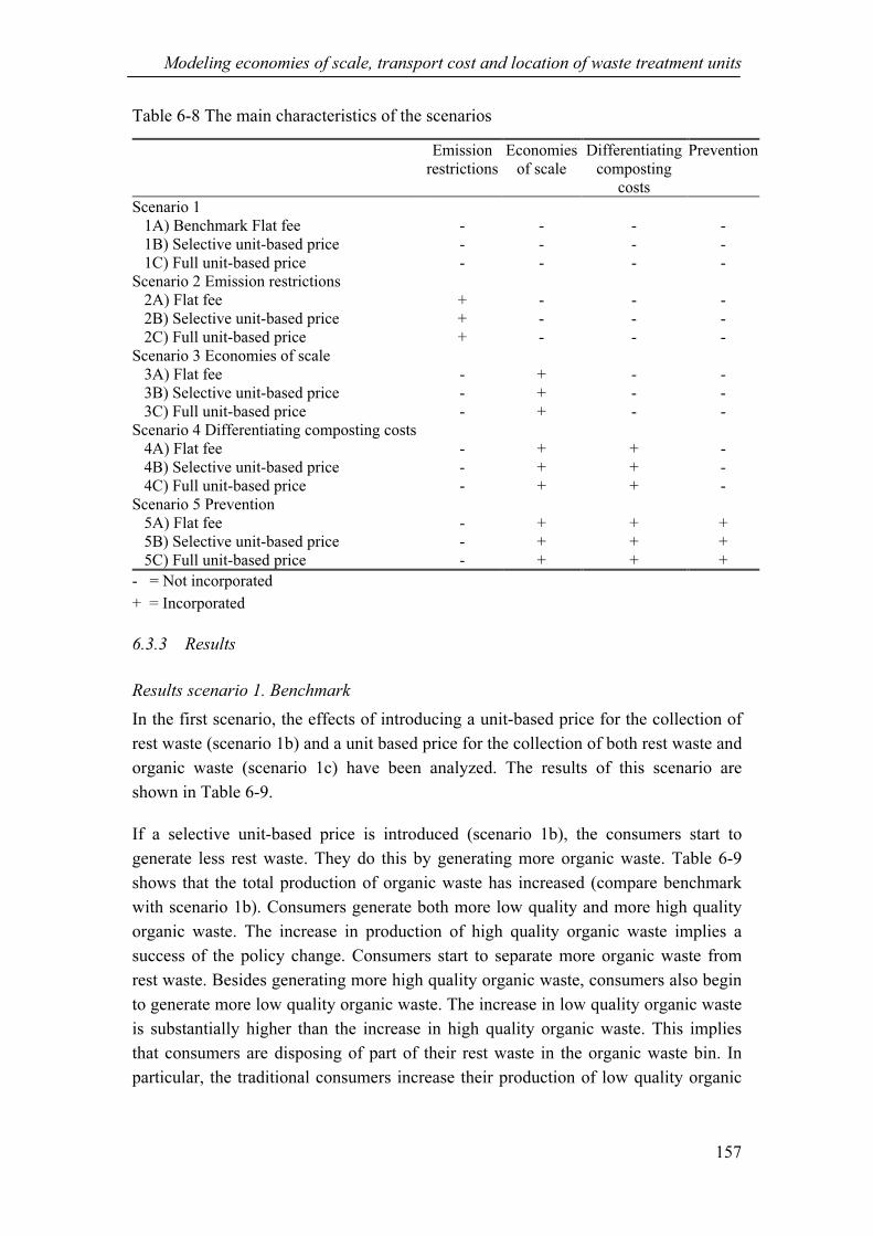
Modeling economies of scale, transport cost and location of waste treatment units
157
Table 6-8 The main characteristics of the scenarios
Emission
restrictions
Economies
of scale
Differentiating
composting
costs
Prevention
Scenario 1
1A) Benchmark Flat fee - - - -
1B) Selective unit-based price - - - -
1C) Full unit-based price - - - -
Scenario 2 Emission restrictions
2A) Flat fee + - - -
2B) Selective unit-based price + - - -
2C) Full unit-based price + - - -
Scenario 3 Economies of scale
3A) Flat fee - + - -
3B) Selective unit-based price - + - -
3C) Full unit-based price - + - -
Scenario 4 Differentiating composting costs
4A) Flat fee - + + -
4B) Selective unit-based price - + + -
4C) Full unit-based price - + + -
Scenario 5 Prevention
5A) Flat fee - + + +
5B) Selective unit-based price - + + +
5C) Full unit-based price - + + +
- = Not incorporated
+ = Incorporated
6.3.3 Results
Results scenario 1. Benchmark
In the first scenario, the effects of introducing a unit-based price for the collection of
rest waste (scenario 1b) and a unit based price for the collection of both rest waste and
organic waste (scenario 1c) have been analyzed. The results of this scenario are
shown in Table 6-9.
If a selective unit-based price is introduced (scenario 1b), the consumers start to
generate less rest waste. They do this by generating more organic waste. Table 6-9
shows that the total production of organic waste has increased (compare benchmark
with scenario 1b). Consumers generate both more low quality and more high quality
organic waste. The increase in production of high quality organic waste implies a
success of the policy change. Consumers start to separate more organic waste from
rest waste. Besides generating more high quality organic waste, consumers also begin
to generate more low quality organic waste. The increase in low quality organic waste
is substantially higher than the increase in high quality organic waste. This implies
that consumers are disposing of part of their rest waste in the organic waste bin. In
particular, the traditional consumers increase their production of low quality organic

Chapter 6
158
waste. Since both low and high quality organic waste are collected together the
overall quality of organic waste stream decreases.
Table 6-9 Results for the main variables under ‘scenario 1 benchmark (in Ktonnes)
and the percentage change as compared to scenario 1a
Variable Scenario1a:
Benchmark case:
Flat fee
Scenario 1b
Selective unit-based
price
Scenario 1c
Full unit-based
price
Consumption good a)
1552 1552 (0%) 1552 (0%)
Collection rest waste 1733 1639 (-5.4%) 1733 (0%)
Collection organic waste 413 507 (22.7%) 413 (0.1%)
Low quality organic waste 85 117 (38.1%) 87 (2.9%)
High quality organic waste 328 390 (18.7%) 326 (-0.7%)
Transport b)
75 75 (0%) 75 (0%)
Composting 413 507 (22.7%) 413 (0.1%)
Small unit 413 507 - 413 -
Medium unit - - - - -
Large unit - - - - -
Incineration 87 90 (4.0%) 87 (0.2%)
Small unit 87 90 - 87 -
Medium unit - - - - -
Large unit - - - - -
Landfilling 1675 1584 (-5.4%) 1675 (0%)
Small unit 1675 1584 - 1675 -
Medium unit - - - - -
Large unit - - - - -
Note: a) Expenditure consumption in million Euros
b) Transport in tonnes per 1000 km
All waste is treated in small waste treatment units, since no economies of scale are
included in this scenario. Given that less rest waste is generated, less waste has to be
incinerated and landfilled. Table 6-9 shows how the quantity of waste landfilled
declines as expected. The quantity of waste incinerated, however, increases because
the residue of the composting process is sent to an incinerator.
The four municipalities differ in the distribution of traditional and green consumers. It
can therefore be expected that the quality of organic waste collected in each of the
municipalities will differ. Table 6-10 shows the quality of organic waste collected in
each of the four municipalities. In all municipalities, the quality of organic waste
decreases. The absolute quality of organic waste is lowest in the two cities
(municipality A and B). In scenario 1b, the percentage change in the quality of the
organic waste stream is comparable for municipality A, B and C. For these
municipalities, the difference in the shares of ‘green’ consumers is not that large.
Thus, although municipality A, the least environmentally friendly municipality,
generates the lowest quality of organic waste, the percentage difference between the
three municipalities is comparable. Only in municipality D, which has the lowest
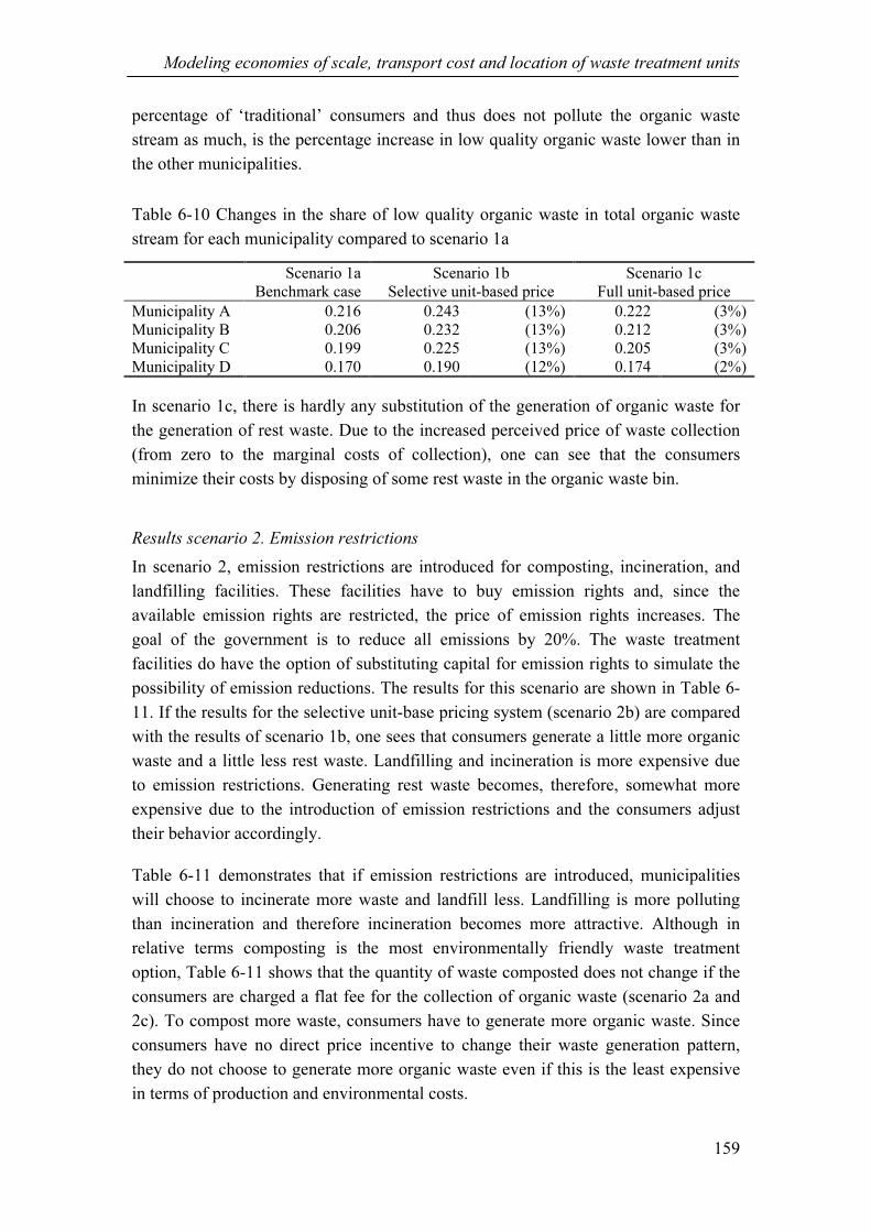
Modeling economies of scale, transport cost and location of waste treatment units
159
percentage of ‘traditional’ consumers and thus does not pollute the organic waste
stream as much, is the percentage increase in low quality organic waste lower than in
the other municipalities.
Table 6-10 Changes in the share of low quality organic waste in total organic waste
stream for each municipality compared to scenario 1a
Scenario 1a
Benchmark case
Scenario 1b
Selective unit-based price
Scenario 1c
Full unit-based price
Municipality A 0.216 0.243 (13%) 0.222 (3%)
Municipality B 0.206 0.232 (13%) 0.212 (3%)
Municipality C 0.199 0.225 (13%) 0.205 (3%)
Municipality D 0.170 0.190 (12%) 0.174 (2%)
In scenario 1c, there is hardly any substitution of the generation of organic waste for
the generation of rest waste. Due to the increased perceived price of waste collection
(from zero to the marginal costs of collection), one can see that the consumers
minimize their costs by disposing of some rest waste in the organic waste bin.
Results scenario 2. Emission restrictions
In scenario 2, emission restrictions are introduced for composting, incineration, and
landfilling facilities. These facilities have to buy emission rights and, since the
available emission rights are restricted, the price of emission rights increases. The
goal of the government is to reduce all emissions by 20%. The waste treatment
facilities do have the option of substituting capital for emission rights to simulate the
possibility of emission reductions. The results for this scenario are shown in Table 6-
11. If the results for the selective unit-base pricing system (scenario 2b) are compared
with the results of scenario 1b, one sees that consumers generate a little more organic
waste and a little less rest waste. Landfilling and incineration is more expensive due
to emission restrictions. Generating rest waste becomes, therefore, somewhat more
expensive due to the introduction of emission restrictions and the consumers adjust
their behavior accordingly.
Table 6-11 demonstrates that if emission restrictions are introduced, municipalities
will choose to incinerate more waste and landfill less. Landfilling is more polluting
than incineration and therefore incineration becomes more attractive. Although in
relative terms composting is the most environmentally friendly waste treatment
option, Table 6-11 shows that the quantity of waste composted does not change if the
consumers are charged a flat fee for the collection of organic waste (scenario 2a and
2c). To compost more waste, consumers have to generate more organic waste. Since
consumers have no direct price incentive to change their waste generation pattern,
they do not choose to generate more organic waste even if this is the least expensive
in terms of production and environmental costs.

Chapter 6
160
Table 6-11 Results for the main variables under ‘emission restriction scenario’ (in
Ktonnes) and the percentage change as compared to scenario 1a
Variable Scenario 2a
Flat fee
Scenario 2b
Selective unit-based
price
Scenario 2c
Full unit-based
price
Consumption good a)
1552 (0.0%) 1552 (0.0%) 1552 (0.0%)
Collection rest waste 1733 (0.0%) 1638 (-5.5%) 1733 (0.0%)
Collection organic waste 413 (0.0%) 508 (23.0%) 413 (0.0%)
Low quality organic waste 85 (0.0%) 117 (38.4%) 87 (3.1%)
High quality organic waste 328 (0.0%) 393 (19.6%) 326 (-0.7%)
Transport b)
75 (0.0%) 75 (0.0%) 75 (0.0%)
Composting 413 (0.0%) 508 (23.0%) 413 (0.0%)
Small unit 413 - 508 - 413 -
Medium unit - - - - - -
Large unit - - - - - -
Incineration 91 (4.7%) 91 (5.2%) 91 (4.7%)
Small unit 91 - 91 - 91 -
Medium unit - - - - - -
Large unit - - - - - -
Landfilling 1671 (-0.2%) 1582 (-5.6%) 1671 (-0.2%)
Small unit 1671 - 1582 - 1671 -
Medium unit - - - - - -
Large unit - - - - - -
Note: a) Expenditure consumption in million Euros
b) Transport in tonnes per 1000 km
Results scenario 3. Economies of scale
In the third scenario, economies of scale have been introduced for the three different
sizes of waste treatment facilities. The results of this scenario are presented in Table
6-12. Due to economies of scale, in scenario 3a, 3b, and 3c respectively,
municipalities opted to transport their waste to a medium sized incinerator instead of a
small one. The economies of scale are smaller for composting units and landfill
facilities and therefore municipalities continue to use the small sized units for these
waste treatment options to avoid higher transport costs. The transport costs to a large
incinerator are too high to be offset by lower incineration costs, so the large
incinerators are not used. Because incineration in a medium sized facility is less
expensive than landfilling municipalities choose to incinerate more and landfill less.
Since they transport waste over a longer distance, the transport costs increase. Part of
the waste is still treated in a small waste incinerator. This is the quantity of waste that
is left as a residue of the composting process14
. All rest waste that is generated by the
private households is sent to the medium sized waste incinerator.
14 It is assumed that composting units only incinerate waste in a small incinerator located near the
composting unit, thus the waste does not require transportation.

Modeling economies of scale, transport cost and location of waste treatment units
161
Table 6-12 Results for the main variables under the ‘economies of scale scenario’ (in
Ktonnes) and the percentage change as compared to scenario 1a
Variable Scenario 3a
Flat fee
Scenario 3b
Selective unit-based
price
Scenario 3c
Full unit-based
price
Consumption good a)
1552 (0.0%) 1552 (0.0%) 1552 (0.0%)
Collection rest waste 1733 (0.0%) 1639 (-5.4%) 1733 (0.0%)
Collection organic waste 413 (0.0%) 507 (22.7%) 413 (0.1%)
Low quality organic waste 85 (0.0%) 117 (38.0%) 87 (2.9%)
High quality organic waste 328 (0.0%) 390 (18.7%) 326 (-0.7%)
Transport b)
79 (5.0%) 79 (4.8%) 79 (5.0%)
Composting 413 (0.0%) 507 (22.7%) 413 (0.1%)
Small unit 413 - 507 - 413 -
Medium unit - - - - - -
Large unit - - - - - -
Incineration 122 (40.3%) 124 (42.6%) 122 (40.9%)
Small unit 29 - 36 - 29 -
Medium unit 93 - 88 - 93 -
Large unit - - - - - -
Landfilling 1642 (-2.0%) 1552 (-7.3%) 1641 (-2.0%)
Small unit 1642 - 1552 1641 -
Medium unit - - - - -
Large unit - - - - -
Note: a) Expenditure consumption in million Euros
b) Transport in tonnes per 1000 km
Results scenario 4. Differentiating composting costs
In scenario 4, different composting costs for low and high quality organic waste have
been introduced. The lower the quality of organic waste, the greater the costs that
have to be incurred in order to actually compost the waste. The results for this
scenario are shown in Table 6-13. Introducing differentiated composting costs has
little effect on the actual waste streams in the flat fee pricing system (scenario 4a).
However, as Table 6-13 illustrates, it does have a strong effect in both the selective
(scenario 4b) and the full unit-based pricing system (scenario 4c). In the selective
unit-based pricing system, the two larger municipalities (A and B) start to transport
their waste to the large sized composting unit. The quality of the organic waste stream
has declined so much that it is cheaper to transport the waste to a large facility than to
a small facility. In the two smaller municipalities (C and D), the share of ‘green’
consumers is larger than in the bigger municipalities and thus the quality of the
organic waste stream does not decline as much. This means that the cost of
composting the waste in a small unit does not increase enough for it to become
attractive to compost the waste in a large unit.
In the full unit-based pricing system, consumers actually start to generate less low
quality organic waste and more high quality organic waste. These results are inherent

Chapter 6
162
to the assumptions of the model. It was assumed that consumers would pay the
marginal costs of waste treatment. Since the marginal costs of treating low quality
organic waste are higher than the marginal costs of treating high quality organic
waste, even if the households need to spend more labor to generate organic waste, the
private households have a direct price incentive to reduce the quantity of low quality
organic waste. In reality, it is unrealistic to assume that the consumers would pay the
exact marginal costs of waste treatment in a full unit-based pricing system. As
explained in Section 6.1, municipalities do not check the quality of organic waste
during collection. Thus it is impossible to charge consumers a higher price for the
collection of low quality organic waste and therefore these results are too optimistic.
Table 6-13 Results for the main variables under the ‘differentiating composting costs
scenario’ (in Ktonnes) and the percentage change as compared to scenario 1a
Variable Scenario 4a
Flat fee
Scenario 4b
Selective unit-based
price
Scenario 4c
Full unit-based
price
Consumption good a)
1552 (0.0%) 1552 (0.0%) 1552 (0.0%)
Collection rest waste 1733 (0.0%) 1639 (-5.5%) 1735 (0.1%)
Collection organic waste 413 (0.0%) 507 (22.7%) 410 (-0.6%)
Low quality organic waste 85 (0.0%) 117 (38.1%) 76 (-10.2%)
High quality organic waste 328 (0.0%) 390 (18.7%) 334 (1.9%)
Transport b)
79 (5.0%) 125 (66.0%) 79 (5.0%)
Composting 413 (0.0%) 507 (22.7%) 410 (-0.6%)
Small unit 413 - 106 - 410 -
Medium unit - - - - - -
Large unit - - 400 - - -
Incineration 122 (40.5%) 128 (47.7%) 119 (37.5%)
Small unit 29 - 40 - 26 -
Medium unit 93 - 88 - 93 -
Large unit - - - - - -
Landfilling 1641 (-2.0%) 1552 (-7.4%) 1643 (-2.0%)
Small unit 1641 - 1552 1643 -
Medium unit - - - - -
Large unit - - - - -
Note: a) Expenditure consumption in million Euros
b) Transport in tonnes per 1000 km
Results scenario 5. Prevention
In the final scenario, the model has been adjusted to incorporate the possibility of
prevention. Consumers can minimize generation of waste by consuming a product,
which generates less waste. The results of this scenario are presented in Table 6-14.
As shown in Table 6-14, the introduction of prevention has little effect on the results.
Consumers only adjust their consumption pattern in a minor fashion. When either a
selective (scenario 5b) or a full unit-based pricing system (scenario 5c) is introduced,

Modeling economies of scale, transport cost and location of waste treatment units
163
consumer start to consume a little bit more of good 2, the consumption of which
generates less waste and a little less of good 1.
Table 6-14 Results for main variable under the ‘prevention scenario’ (in Ktonnes) and
the percentage change as compared to the adjusted benchmark case
Variable Scenario 5a
Flat fee
Scenario 5b
Selective unit-based
price
Scenario 5c
Full unit-based
price
Consumption good 1 a)
1008 (0.0%) 1007 (-0.2%) 1007 (-0.3%)
Consumption good 2 a)
543 (0.0%) 545 (0.4%) 546 (0.4%)
Collection rest waste 1733 (0.0%) 1637 (-5.5%) 1733 (0.1%)
Collection organic waste 413 (0.0%) 506 (22.6%) 410 (-0.6%)
Low quality organic waste 85 (0.0%) 117 (38.0%) 76 (-10.2%)
High quality organic waste 328 (0.0%) 389 (18.6%) 334 (1.8%)
Transport b)
79 (5.0%) 125 (65.8%) 79 (5.0%)
Composting 413 (0.0%) 506 (22.6%) 410 (-0.6%)
Small unit 413 - 106 - 410 -
Medium unit - - - - - -
Large unit - - 400 - - -
Incineration 122 (40.6%) 128 (46.9%) 119 (37.1%)
Small unit 29 - 41 - 26 -
Medium unit 93 - 88 - 93 -
Large unit - - - - - -
Landfilling 1641 (-2.0%) 1552 (-7.4%) 1642 (-2.0%)
Small unit 1641 - 1552 1642 -
Medium unit - - - - -
Large unit - - - - -
Note: a) Expenditure consumption in million Euros
b) Transport in tonnes per 1000 km
The price incentive by increasing the marginal price of waste generation, however, is
too small to have a large impact on the consumption patterns of private households.
These results are not completely unexpected, practical experience has shown that
although unit-based pricing stimulates more waste separation, it does not or hardly
stimulates prevention (Linderhof et al., 2001). The price incentive is simply too small
to change consumption patterns.
6.3.4 Comparing the different pricing mechanisms
Based on the fifth scenario, the most complex scenario, it is possible to make an
extensive comparison between the three different pricing systems. As shown in
Section 6.3.3, the total quantity of waste generated is hardly affected by the
introduction of either a selective unit based pricing system or a full unit-based pricing
system. The composition of the waste stream, however, did differ between the three
different pricing systems. This is illustrated in Figure 6-3.

Chapter 6
164
60%
65%
70%
75%
80%
85%
90%
95%
100%
Flat fee Selective
unit-based
price
Full unit-
based price
Per
centa
ge
of
each
was
te c
ateg
ory
.
in t
ota
l w
aste
str
eam
high quality organic
waste
low quality organic
waste
rest waste
Figure 6-3 The composition of the waste stream for the three different pricing
mechanisms
A selective unit-based pricing system causes the most significant substitution of
organic waste for rest waste. A full unit-based pricing system has hardly any effect on
the quantity of rest waste and organic waste generated. In the selective unit-based
pricing system, however, there is also a substantial increase in the quantity of low
quality organic waste. Since consumers do not need to fear any penalties, they start to
pollute the organic waste stream with rest waste. This waste leakage effect greatly
increases the cost of composting organic waste. In a full unit-based pricing system,
there is barely any incentive for the consumers to start polluting waste; waste leakage
is, therefore, not such a big problem in the full unit-based pricing system.
The cost of waste treatment differed significantly between the different pricing
systems. This is shown in Figure 6-4.
166.7157.6
166.8
34.3
27.3
32.3
28.4
44.828.4
10.2
11.09.9
135.0
155.0
175.0
195.0
215.0
235.0
Flat fee Selective unit-
based price
Full unit-based
price
Co
sts
(in
mil
lio
n E
uro
)
Transport
Composting
Incineration
Landfilling
Figure 6-4 The total costs of waste treatment for the three different pricing
mechanisms

Modeling economies of scale, transport cost and location of waste treatment units
165
Figure 6-5 Transport of organic and rest waste for each municipality
Location choice composting of organic waste
Location choice landfilling of rest waste
Location choice incineration of rest waste
Municipality Large WTU Medium WTU Small WTU
Transport wasteNote: WTU stands for waste treatment unit.
Flat fee Selective unit-based price
A
C D
B
C D
160
ktons
41
ktons
41
ktons
165
ktons
41
ktons
41
ktons
198
ktons
202
ktons
A B
A
C D
BA
C D
B
37 ktons
9 ktons
37 ktons
9 ktons
35 ktons
9 ktons
35 ktons
9 ktons
Flat fee Selective unit-based price
A
C D
B A
C D
B
661
ktons
657
ktons
163
ktons
159
ktons
155
ktons
151
ktons
625
ktons
621
ktons
Flat fee Selective unit-based price

Chapter 6
166
In a flat fee pricing system, all organic waste is treated in a small composting unit.
Households generate mostly high quality organic waste, but also some low quality
organic waste. Composting of low quality organic waste is expensive, especially if it
is treated in a small composting unit. Although it is quite expensive for the
municipalities to compost low quality organic waste in a small composting unit, the
increased costs of composting are not so high that they would offset the costs of
transporting the waste to a large composting unit. If a selective unit-based pricing
system is introduced the situation is quite different. In the larger municipalities, the
quality of the organic waste stream declines so much that these municipalities choose
to transport the waste to a large composting unit. This results in sharply increasing
transport costs and decreasing composting costs, as shown in Figure 6-4. An
illustration of the transport flows of waste in a flat fee pricing system and a selective
unit based pricing system is given in Figure 6-5 as shown on the previous page.
The distribution of costs in the full unit-based pricing system was quite similar to the
distribution of costs in the flat fee pricing system. The overall costs spent on waste
treatment were highest in the selective unit-based pricing system, due to waste
leakage effect.
Finally, it is also interesting to compare the emissions of CO2, NOX, and CH4 in the
different pricing systems. These emissions are shown in Figure 6-6.
100%
107%
100%
98%99%
117%
100%
96%
100%
90.00%
95.00%
100.00%
105.00%
110.00%
115.00%
120.00%
Flat fee Selective unit-based
price
Full unit-based price
Ind
ex (
ben
chm
ark
=1
00
%)
CO2NOXCH4
Figure 6-6 Normalized CO2, NOX, and CH4 emissions caused by waste treatment and
transport as compared to flat fee scenario (flat fee =100%)
In the selective unit-based pricing system, both CO2-emissions and NOX-emissions
increase. This is caused by two factors. Firstly, the transport of waste increases
sharply in the selective unit-based pricing system. As transport lead to both CO2 and

Modeling economies of scale, transport cost and location of waste treatment units
167
NOX emissions, these emissions increase. Secondly, in the selective unit-based
pricing system, more low quality organic waste is generated. Composting low quality
organic waste creates a residue, which is incinerated. Incineration of this residue
results in extra CO2-emissions and NOX-emissions. A positive effect of the selective
unit-based pricing system is that it reduces the quantity of waste that is landfilled, thus
generating substantially fewer CH4 emissions.
The emissions in the full unit-based pricing system are slightly lower than the
emissions in the flat fee pricing system. The full unit-based pricing system is slightly
better for the environment than the flat fee-pricing scheme. Based on the results
presented in Figure 6-6, one may jump to the conclusion that a selective unit-based
pricing scheme is worse for the environment than either of the two other pricing
schemes; however this would depend on an economic valuation of the damage caused
by CO2, NOX, and CH4 emissions. It is, however, clear that in our model the selective
unit-based pricing scheme aggravates the problem of acidification.
6.4 Discussion and conclusions
In this chapter, we have demonstrated how the spatial aspects of the waste
management problem can be included in a general equilibrium framework. A general
equilibrium model is a suitable tool for modeling the interactions between the choices
that the consumers make about the quality and quantity of waste they generate, the
choices that the municipalities make about how and where the waste should be treated
and the costs of waste treatment.
In a stylized example with numerical data based on the Randstad in 2000, we have
shown how the optimal waste treatment choice and the choice for the optimal location
of the waste treatment unit can be influenced by a policy change for the consumers.
The results show that if a unit-based price for the collection of rest waste was
implemented, the consumers would start to generate less rest waste and more organic
waste. This is a positive effect. More waste will be composted, which will result in
lower waste treatment costs and less environmental damage. There is, however, also a
negative effect. The quality of organic waste would be seriously affected. The
‘traditional’ consumers in particular would start to dispose of rest waste in the organic
waste bin, thus polluting the organic waste stream. Since the quality of the organic
waste stream greatly declines, it consequently becomes far more expensive to
compost the waste. If the quality of organic waste is too poor, part of the waste cannot
be composted. Instead it must be incinerated. This means that the environmental gains
will be much smaller than can be expected based on the reduction in waste generation
without considering waste leakage. Although less rest waste is incinerated or
landfilled, more organic waste has to be composted, thus leading to more CO2
emissions.
Chapter 6
168
The results of the numerical example show that in the larger municipalities the quality
of the organic waste stream declines so much that waste will have to be treated in a
large composting facility instead of a small one, thus incurring more transport costs.
In this example, it would not be cost-effective to introduce a unit-based price for the
collection of rest waste in larger municipalities since the increased costs of
composting due to the decrease in the quality of organic waste are not offset by the
benefits of the lower generation of rest waste. Only in small municipalities, with a
relatively large number of green consumers, will unit-based pricing for the collection
of rest waste be interesting.
The introduction of unit-based pricing on the collection of rest waste as well as on the
collection of organic waste creates fewer problems with regard to waste leakage. This
policy option, however, does not stimulate the consumer to separate its waste.
Therefore, there are hardly any benefits of introducing such a pricing scheme, given
the restrictions of the model. If we consider that introducing such a pricing scheme
will probably involve high transaction costs, it would not be advisable for
municipalities to consider this policy option. It is important to bear in mind that only
the option of substituting rest waste for organic waste has been analyzed. Particularly
in smaller municipalities, consumers will have the option of reducing their organic
waste stream by composting it at home. The full unit-based pricing scheme may well
provide an incentive for more waste to be composted at home, thus reducing the
organic and rest waste streams. Municipalities with a relatively large share of
consumers that are not able to engage in home composting, however, do not need to
consider this kind of pricing scheme.
Naturally, there are a number of uncertainties in this analysis. Several extensions,
such as, for example, home composting, recycling, detailed modeling of prevention or
more categories of waste, could be added to the model to make it more realistic. This
analysis, however, demonstrates that the interactions between the quality of waste, the
method of waste treatment, transport costs, the presence of economies of scale and
environmental damages can have significant implications for the success of a policy
change and therefore should be considered when deciding on which policy should be
implemented in order to minimize waste generation.

Modeling economies of scale, transport cost and location of waste treatment units
169
15
52
.31
55
2.1
15
52
.31
55
2.3
15
52
.11
55
2.3
15
52
.31
55
2.1
15
52
.31
55
2.1
15
51
.91
55
2.1
10
08
.91
00
6.7
10
06
.5
--
--
--
--
--
--
54
3.3
54
5.2
54
5.7
17
33
.01
63
8.9
17
32
.81
73
3.2
16
37
.71
73
2.7
17
33
.01
63
9.0
17
32
.71
73
2.5
16
38
.61
73
5.1
17
32
.51
63
7.3
17
33
.2
41
3.0
50
6.9
41
3.2
41
2.8
50
8.0
41
3.3
41
3.0
50
6.7
41
3.2
41
3.0
50
6.6
41
0.4
41
3.0
50
6.2
41
0.4
Lo
w q
ual
ity
84
.81
17
.18
7.3
84
.71
17
.48
7.4
84
.81
17
.08
7.3
84
.81
17
.07
6.1
84
.81
17
.07
6.1
Hig
h q
ual
ity
32
8.3
38
9.8
32
6.0
32
8.1
39
2.6
32
5.9
32
8.2
38
9.7
32
6.0
32
8.2
38
9.6
33
4.3
32
8.2
38
9.2
33
4.3
75
.17
5.1
75
.17
5.1
75
.17
5.1
78
.97
8.7
78
.97
8.9
12
4.7
78
.97
8.9
12
4.6
78
.8
41
3.0
50
6.9
41
3.2
41
2.8
50
8.0
41
3.3
41
3.0
50
6.7
41
3.2
41
3.0
50
6.6
41
0.4
41
3.0
50
6.2
41
0.4
Sm
all
un
it4
13
.05
06
.94
13
.24
12
.85
08
.04
13
.34
13
.05
06
.74
13
.24
13
.01
06
.34
10
.44
13
.01
06
.24
10
.4
Med
ium
un
it-
--
--
--
--
--
--
--
Lar
ge
un
it-
--
--
--
--
-4
00
.3-
-4
00
.0-
86
.79
0.2
86
.99
0.7
91
.29
0.5
12
1.6
12
3.6
12
2.2
12
1.8
12
8.0
11
9.2
12
1.9
12
8.0
11
8.9
Sm
all
un
it8
6.7
90
.28
6.9
90
.79
1.2
90
.52
8.9
35
.52
8.9
28
.93
9.9
25
.82
8.9
40
.52
6.3
Med
ium
un
it-
--
--
-9
2.7
88
.19
3.2
92
.98
8.1
93
.49
3.0
87
.59
2.6
Lar
ge
un
it-
--
--
--
--
--
--
--
16
75
.21
58
4.2
16
74
.81
67
1.4
15
82
.11
67
1.2
16
41
.81
55
2.4
16
41
.01
64
1.2
15
52
.01
64
3.4
16
41
.11
55
2.0
16
41
.8
Sm
all
un
it1
67
5.2
15
84
.21
67
4.8
16
71
.41
58
2.1
16
71
.21
64
1.8
15
52
.41
64
1.0
16
41
.21
55
2.0
16
43
.41
64
1.1
15
52
.01
64
1.8
Med
ium
un
it-
--
--
--
--
--
--
--
Lar
ge
un
it-
--
--
--
--
--
--
--
No
te:
a)E
xp
end
itu
re c
on
sum
pti
on
in
mil
lio
n e
uro
s
Fu
ll
un
it-b
ased
pri
ce
Fu
ll
un
it-b
ased
pri
ce
Fu
ll
un
it-b
ased
pri
ce
Fu
ll
un
it-b
ased
pri
ce
Fu
ll
un
it-b
ased
pri
ce
Co
mp
ost
ing
Inci
ner
atio
n
Lan
dfi
llin
g
Appen
dix
6-A
.1 R
esult
s m
ain v
aria
ble
s fo
r ea
ch s
cen
ario
(in
1000 t
onnes
)
Co
nsu
mp
tio
n g
oo
d 2a)
Co
llec
tio
n r
est
was
te
Co
llec
tio
n o
rgan
ic
Tra
nsp
ort
Sel
ecti
ve
un
it-b
ased
pri
ce
Fla
t fe
eS
elec
tive
un
it-b
ased
pri
ce
Co
nsu
mp
tio
n g
oo
d 1a)
Sce
na
rio
5.
Pre
ven
tio
n
Var
iab
leF
lat
fee
Sel
ecti
ve
un
it-b
ased
pri
ce
Fla
t fe
eS
elec
tive
un
it-b
ased
pri
ce
Fla
t fe
eS
elec
tive
un
it-b
ased
pri
ce
Fla
t fe
e
Sce
na
rio
3.
Eco
no
mie
s o
f sc
ale
Scen
ario
4.
Dif
fere
nti
ati
ng
co
mp
ost
ing
Scen
ario
1.
Ben
chm
ark
Scen
ario
2.
Em
issi
on
res
tric
tio
ns
15
52
.31
55
2.1
15
52
.31
55
2.3
15
52
.11
55
2.3
15
52
.31
55
2.1
15
52
.31
55
2.1
15
51
.91
55
2.1
10
08
.91
00
6.7
10
06
.5
--
--
--
--
--
--
54
3.3
54
5.2
54
5.7
17
33
.01
63
8.9
17
32
.81
73
3.2
16
37
.71
73
2.7
17
33
.01
63
9.0
17
32
.71
73
2.5
16
38
.61
73
5.1
17
32
.51
63
7.3
17
33
.2
41
3.0
50
6.9
41
3.2
41
2.8
50
8.0
41
3.3
41
3.0
50
6.7
41
3.2
41
3.0
50
6.6
41
0.4
41
3.0
50
6.2
41
0.4
Lo
w q
ual
ity
84
.81
17
.18
7.3
84
.71
17
.48
7.4
84
.81
17
.08
7.3
84
.81
17
.07
6.1
84
.81
17
.07
6.1
Hig
h q
ual
ity
32
8.3
38
9.8
32
6.0
32
8.1
39
2.6
32
5.9
32
8.2
38
9.7
32
6.0
32
8.2
38
9.6
33
4.3
32
8.2
38
9.2
33
4.3
75
.17
5.1
75
.17
5.1
75
.17
5.1
78
.97
8.7
78
.97
8.9
12
4.7
78
.97
8.9
12
4.6
78
.8
41
3.0
50
6.9
41
3.2
41
2.8
50
8.0
41
3.3
41
3.0
50
6.7
41
3.2
41
3.0
50
6.6
41
0.4
41
3.0
50
6.2
41
0.4
Sm
all
un
it4
13
.05
06
.94
13
.24
12
.85
08
.04
13
.34
13
.05
06
.74
13
.24
13
.01
06
.34
10
.44
13
.01
06
.24
10
.4
Med
ium
un
it-
--
--
--
--
--
--
--
Lar
ge
un
it-
--
--
--
--
-4
00
.3-
-4
00
.0-
86
.79
0.2
86
.99
0.7
91
.29
0.5
12
1.6
12
3.6
12
2.2
12
1.8
12
8.0
11
9.2
12
1.9
12
8.0
11
8.9
Sm
all
un
it8
6.7
90
.28
6.9
90
.79
1.2
90
.52
8.9
35
.52
8.9
28
.93
9.9
25
.82
8.9
40
.5
15
52
.31
55
2.1
15
52
.31
55
2.3
15
52
.11
55
2.3
15
52
.31
55
2.1
15
52
.31
55
2.1
15
51
.91
55
2.1
10
08
.91
00
6.7
10
06
.5
--
--
--
--
--
--
54
3.3
54
5.2
54
5.7
17
33
.01
63
8.9
17
32
.81
73
3.2
16
37
.71
73
2.7
17
33
.01
63
9.0
17
32
.71
73
2.5
16
38
.61
73
5.1
17
32
.51
63
7.3
17
33
.2
41
3.0
50
6.9
41
3.2
41
2.8
50
8.0
41
3.3
41
3.0
50
6.7
41
3.2
41
3.0
50
6.6
41
0.4
41
3.0
50
6.2
41
0.4
Lo
w q
ual
ity
84
.81
17
.18
7.3
84
.71
17
.48
7.4
84
.81
17
.08
7.3
84
.81
17
.07
6.1
84
.81
17
.07
6.1
Hig
h q
ual
ity
32
8.3
38
9.8
32
6.0
32
8.1
39
2.6
32
5.9
32
8.2
38
9.7
32
6.0
32
8.2
38
9.6
33
4.3
32
8.2
38
9.2
33
4.3
75
.17
5.1
75
.17
5.1
75
.17
5.1
78
.97
8.7
78
.97
8.9
12
4.7
78
.97
8.9
12
4.6
78
.8
41
3.0
50
6.9
41
3.2
41
2.8
50
8.0
41
3.3
41
3.0
50
6.7
41
3.2
41
3.0
50
6.6
41
0.4
41
3.0
50
6.2
41
0.4
Sm
all
un
it4
13
.05
06
.94
13
.24
12
.85
08
.04
13
.34
13
.05
06
.74
13
.24
13
.01
06
.34
10
.44
13
.01
06
.24
10
.4
Med
ium
un
it-
--
--
--
--
--
--
--
Lar
ge
un
it-
--
--
--
--
-4
00
.3-
-4
00
.0-
86
.79
0.2
86
.99
0.7
91
.29
0.5
12
1.6
12
3.6
12
2.2
12
1.8
12
8.0
11
9.2
12
1.9
12
8.0
11
8.9
Sm
all
un
it8
6.7
90
.28
6.9
90
.79
1.2
90
.52
8.9
35
.52
8.9
28
.93
9.9
25
.82
8.9
40
.52
6.3
Med
ium
un
it-
--
--
-9
2.7
88
.19
3.2
92
.98
8.1
93
.49
3.0
87
.59
2.6
Lar
ge
un
it-
--
--
--
--
--
--
--
16
75
.21
58
4.2
16
74
.81
67
1.4
15
82
.11
67
1.2
16
41
.81
55
2.4
16
41
.01
64
1.2
15
52
.01
64
3.4
16
41
.11
55
2.0
16
41
.8
Sm
all
un
it1
67
5.2
15
84
.21
67
4.8
16
71
.41
58
2.1
16
71
.21
64
1.8
15
52
.41
64
1.0
16
41
.21
55
2.0
16
43
.41
64
1.1
15
52
.01
64
1.8
Med
ium
un
it-
--
--
--
--
--
--
--
Lar
ge
un
it-
--
--
--
--
--
--
--
No
te:
a)E
xp
end
itu
re c
on
sum
pti
on
in
mil
lio
n e
uro
s
Fu
ll
un
it-b
ased
pri
ce
Fu
ll
un
it-b
ased
pri
ce
Fu
ll
un
it-b
ased
pri
ce
Fu
ll
un
it-b
ased
pri
ce
Fu
ll
un
it-b
ased
pri
ce
Co
mp
ost
ing
Inci
ner
atio
n
Lan
dfi
llin
g
Appen
dix
6-A
.1 R
esult
s m
ain v
aria
ble
s fo
r ea
ch s
cen
ario
(in
1000 t
onnes
)
Co
nsu
mp
tio
n g
oo
d 2a)
Co
llec
tio
n r
est
was
te
Co
llec
tio
n o
rgan
ic
Tra
nsp
ort
Sel
ecti
ve
un
it-b
ased
pri
ce
Fla
t fe
eS
elec
tive
un
it-b
ased
pri
ce
Co
nsu
mp
tio
n g
oo
d 1a)
Sce
na
rio
5.
Pre
ven
tio
n
Var
iab
leF
lat
fee
Sel
ecti
ve
un
it-b
ased
pri
ce
Fla
t fe
eS
elec
tive
un
it-b
ased
pri
ce
Fla
t fe
eS
elec
tive
un
it-b
ased
pri
ce
Fla
t fe
e
Sce
na
rio
3.
Eco
no
mie
s o
f sc
ale
Scen
ario
4.
Dif
fere
nti
ati
ng
co
mp
ost
ing
Scen
ario
1.
Ben
chm
ark
Scen
ario
2.
Em
issi
on
res
tric
tio
ns

Chapter 6
170
22
4.6
21
9.9
22
4.6
24
1.9
24
0.1
24
1.8
22
3.9
21
9.3
22
3.9
23
9.6
24
0.8
23
7.5
23
9.6
24
0.7
23
7.3
Co
sts
com
po
stin
g1
8.6
22
.81
8.6
20
.82
6.3
20
.81
8.6
22
.81
8.6
34
.32
7.3
32
.33
4.3
27
.33
2.3
Co
sts
inci
ner
atio
n8
.89
.28
.81
0.3
11
10
.31
0.2
10
.51
0.2
10
.21
0.9
9.9
10
.21
19
.9
Co
sts
lan
dfi
llin
g1
70
.21
60
.91
70
.11
83
.71
75
.81
83
.71
66
.81
57
.71
66
.71
66
.71
57
.61
66
.91
66
.71
57
.61
66
.8
Co
sts
tran
spo
rt2
72
72
72
72
72
72
8.4
28
.32
8.4
28
.44
4.9
28
.42
8.4
44
.82
8.4
CO
24
29
51
44
58
64
30
36
.63
49
05
.73
49
05
.73
48
55
.75
93
67
.96
03
00
59
64
2.8
59
46
0.7
63
88
1.5
58
26
9.2
59
51
6.2
63
56
9.5
58
12
4.4
NO
X9
4.1
95
.79
4.2
80
.68
0.6
80
.71
09
.31
10
.21
09
.51
09
.31
28
.41
08
.31
09
.41
28
.11
08
.1
CH
41
84
83
17
75
8.3
18
47
9.6
14
78
6.6
14
78
6.6
14
78
6.6
18
13
5.3
17
42
6.4
18
12
7.8
18
12
91
74
22
.31
81
46
18
12
7.8
17
41
41
81
28
.6
15
52
.00
.0%
0.0
%0
.0%
0.0
%0
.0%
0.0
%0
.0%
0.0
%0
.0%
0.0
%0
.0%
0.0
%a)
-0.2
%a)
-0.3
%a)
--
--
--
--
--
--
0.0
%a)
0.4
%a)
0.4
%a)
17
33
.0-5
.4%
0.0
%0
.0%
-5.5
%0
.0%
0.0
%-5
.4%
0.0
%0
.0%
-5.5
%0
.1%
0.0
%-5
.5%
0.0
%
41
3.0
22
.7%
0.1
%0
.0%
23
.0%
0.0
%0
.0%
22
.7%
0.1
%0
.0%
22
.7%
-0.6
%0
.0%
22
.6%
-0.6
%
Lo
w q
ual
ity
84
.83
8.1
%2
.9%
0.0
%3
8.4
%3
.1%
0.0
%3
8.0
%2
.9%
0.0
%3
8.1
%-1
0.2
%0
.0%
38
.0%
-10
.2%
Hig
h q
ual
ity
32
8.3
18
.7%
-0.7
%0
.0%
19
.6%
-0.7
%0
.0%
18
.7%
-0.7
%0
.0%
18
.7%
1.9
%0
.0%
18
.6%
1.8
%
75
.10
.0%
0.0
%0
.0%
0.0
%0
.0%
5.0
%4
.8%
5.0
%5
.0%
66
.0%
5.0
%5
.0%
65
.8%
4.9
%
41
3.0
22
.7%
0.1
%0
.0%
23
.0%
0.0
%0
.0%
22
.7%
0.1
%0
.0%
22
.7%
0.0
%0
.0%
22
.6%
-0.6
%
86
.74
.0%
0.2
%4
.7%
5.2
%4
.7%
40
.3%
42
.6%
40
.9%
40
.5%
47
.7%
37
.5%
40
.6%
46
.9%
37
.1%
16
75
.2-5
.4%
0.0
%-0
.2%
-5.6
%-0
.2%
-2.0
%-7
.3%
-2.0
%-2
.0%
-7.4
%-2
.0%
-2.0
%-7
.4%
-2.0
%
a) p
erce
nta
ge
chan
ge
as c
om
pare
d t
o t
he
adju
sted
ben
chm
ark
cas
e. S
ee s
ecti
on
6.3
.2 f
or
mo
re i
nfo
rmat
ion
.
Fu
ll
un
it-b
ased
pri
ce
Fu
ll
un
it-b
ased
pri
ce
Fu
ll
un
it-b
ased
pri
ce
Fu
ll
un
it-b
ased
pri
ce
Fu
ll
un
it-b
ased
pri
ce
Fu
ll
un
it-b
ased
pri
ce
Fu
ll
un
it-b
ased
pri
ce
Fu
ll
un
it-b
ased
pri
ce
Fu
ll
un
it-b
ased
pri
ce
Fu
ll
un
it-b
ased
pri
ce
Appen
dix
6-A
.3 R
esult
s m
ain v
aria
ble
s as
per
centa
ges
com
par
ed t
o t
he
ben
chm
ark c
ase
Tra
nsp
ort
Co
mp
ost
ing
Inci
ner
atio
n
Lan
dfi
llin
g
Co
nsu
mp
tio
n g
oo
d 1
Co
nsu
mp
tio
n g
oo
d 2
Co
llec
tio
n r
est
was
te
Co
llec
tio
n o
rgan
ic
Fla
t fe
eS
elec
tive
un
it-b
ased
pri
ce
Fla
t fe
eS
elec
tive
un
it-b
ased
pri
ce
Dif
fere
nti
ati
ng
co
mp
ost
ing
Sce
na
rio
5.
Pre
ven
tio
n
Var
iab
leF
lat
fee
Sel
ecti
ve
un
it-b
ased
pri
ce
Fla
t fe
eS
elec
tive
un
it-b
ased
pri
ce
Fla
t fe
eS
elec
tive
un
it-b
ased
pri
ce
To
tal
emis
sio
ns
Appen
dix
6-A
.2 T
ota
l co
sts
and e
mis
sions
was
te t
reat
men
t (c
ost
s in
mil
lion e
uro
s an
d e
mis
sions
in t
ons.
)
Scen
ario
1.
Ben
chm
ark
Scen
ario
2.
Em
issi
on
res
tric
tio
ns
Sce
na
rio
3.
Eco
no
mie
s o
f sc
ale
Sce
na
rio
4.
Sel
ecti
ve
un
it-b
ased
pri
ce
Fla
t fe
eS
elec
tive
un
it-b
ased
pri
ce
To
tal
cost
s w
aste
Sce
na
rio
5.
Pre
ven
tio
n
Var
iab
leF
lat
fee
Sel
ecti
ve
un
it-b
ased
pri
ce
Fla
t fe
eS
elec
tive
un
it-b
ased
pri
ce
Fla
t fe
eS
elec
tive
un
it-b
ased
pri
ce
Fla
t fe
e
Sce
na
rio
3.
Eco
no
mie
s o
f sc
ale
Sce
na
rio
4.
Dif
fere
nti
ati
ng
co
mp
ost
ing
Scen
ario
1.
Ben
chm
ark
Scen
ario
2.
Em
issi
on
res
tric
tio
ns
22
4.6
21
9.9
22
4.6
24
1.9
24
0.1
24
1.8
22
3.9
21
9.3
22
3.9
23
9.6
24
0.8
23
7.5
23
9.6
24
0.7
23
7.3
Co
sts
com
po
stin
g1
8.6
22
.81
8.6
20
.82
6.3
20
.81
8.6
22
.81
8.6
34
.32
7.3
32
.33
4.3
27
.33
2.3
Co
sts
inci
ner
atio
n8
.89
.28
.81
0.3
11
10
.31
0.2
10
.51
0.2
10
.21
0.9
9.9
10
.21
19
.9
Co
sts
lan
dfi
llin
g1
70
.21
60
.91
70
.11
83
.71
75
.81
83
.71
66
.81
57
.71
66
.71
66
.71
57
.61
66
.91
66
.71
57
.61
66
.8
Co
sts
tran
spo
rt2
72
72
72
72
72
72
8.4
28
.32
8.4
28
.44
4.9
28
.42
8.4
44
.82
8.4
CO
24
29
51
44
58
64
30
36
.63
49
05
.73
49
05
.73
48
55
.75
93
67
.96
03
00
59
64
2.8
59
46
0.7
63
88
1.5
58
26
9.2
59
51
6.2
63
56
9.5
58
12
4.4
NO
X9
4.1
95
.79
4.2
80
.68
0.6
80
.71
09
.31
10
.21
09
.51
09
.31
28
.41
08
.31
09
.41
28
.11
08
.1
CH
41
84
83
17
75
8.3
18
47
9.6
14
78
6.6
14
78
6.6
14
78
6.6
18
13
5.3
17
42
6.4
18
12
7.8
18
12
91
74
22
.31
81
46
18
12
7.8
17
41
41
81
28
.6
15
52
.00
.0%
0.0
%0
.0%
0.0
%0
.0%
0.0
%0
.0%
0.0
%0
.0%
0.0
%0
.0%
0.0
%a)
-0.2
%a)
-0.3
%a)
--
--
--
--
--
--
0.0
%a)
0.4
%a)
0.4
%a)
17
33
.0-5
.4%
0.0
%0
.0%
-5.5
%0
.0%
0.0
%-5
.4%
0.0
%0
.0%
-5.5
%0
.1%
0.0
%-5
.5%
0.0
%
41
3.0
22
.7%
0.1
%0
.0%
23
.0%
0.0
%0
.0%
22
.7%
0.1
%0
.0%
22
.7%
-0.6
%0
.0%
22
.6%
-0.6
%
Lo
w q
ual
ity
84
.83
8.1
%2
.9%
0.0
%3
8.4
%3
.1%
22
4.6
21
9.9
22
4.6
24
1.9
24
0.1
24
1.8
22
3.9
21
9.3
22
3.9
23
9.6
24
0.8
23
7.5
23
9.6
24
0.7
23
7.3
Co
sts
com
po
stin
g1
8.6
22
.81
8.6
20
.82
6.3
20
.81
8.6
22
.81
8.6
34
.32
7.3
32
.33
4.3
27
.33
2.3
Co
sts
inci
ner
atio
n8
.89
.28
.81
0.3
11
10
.31
0.2
10
.51
0.2
10
.21
0.9
9.9
10
.21
19
.9
Co
sts
lan
dfi
llin
g1
70
.21
60
.91
70
.11
83
.71
75
.81
83
.71
66
.81
57
.71
66
.71
66
.71
57
.61
66
.91
66
.71
57
.61
66
.8
Co
sts
tran
spo
rt2
72
72
72
72
72
72
8.4
28
.32
8.4
28
.44
4.9
28
.42
8.4
44
.82
8.4
CO
24
29
51
44
58
64
30
36
.63
49
05
.73
49
05
.73
48
55
.75
93
67
.96
03
00
59
64
2.8
59
46
0.7
63
88
1.5
58
26
9.2
59
51
6.2
63
56
9.5
58
12
4.4
NO
X9
4.1
95
.79
4.2
80
.68
0.6
80
.71
09
.31
10
.21
09
.51
09
.31
28
.41
08
.31
09
.41
28
.11
08
.1
CH
41
84
83
17
75
8.3
18
47
9.6
14
78
6.6
14
78
6.6
14
78
6.6
18
13
5.3
17
42
6.4
18
12
7.8
18
12
91
74
22
.31
81
46
18
12
7.8
17
41
41
81
28
.6
15
52
.00
.0%
0.0
%0
.0%
0.0
%0
.0%
0.0
%0
.0%
0.0
%0
.0%
0.0
%0
.0%
0.0
%a)
-0.2
%a)
-0.3
%a)
--
--
--
--
--
--
0.0
%a)
0.4
%a)
0.4
%a)
17
33
.0-5
.4%
0.0
%0
.0%
-5.5
%0
.0%
0.0
%-5
.4%
0.0
%0
.0%
-5.5
%0
.1%
0.0
%-5
.5%
0.0
%
41
3.0
22
.7%
0.1
%0
.0%
23
.0%
0.0
%0
.0%
22
.7%
0.1
%0
.0%
22
.7%
-0.6
%0
.0%
22
.6%
-0.6
%
Lo
w q
ual
ity
84
.83
8.1
%2
.9%
0.0
%3
8.4
%3
.1%
0.0
%3
8.0
%2
.9%
0.0
%3
8.1
%-1
0.2
%0
.0%
38
.0%
-10
.2%
Hig
h q
ual
ity
32
8.3
18
.7%
-0.7
%0
.0%
19
.6%
-0.7
%0
.0%
18
.7%
-0.7
%0
.0%
18
.7%
1.9
%0
.0%
18
.6%
1.8
%
75
.10
.0%
0.0
%0
.0%
0.0
%0
.0%
5.0
%4
.8%
5.0
%5
.0%
66
.0%
5.0
%5
.0%
65
.8%
4.9
%
41
3.0
22
.7%
0.1
%0
.0%
23
.0%
0.0
%0
.0%
22
.7%
0.1
%0
.0%
22
.7%
0.0
%0
.0%
22
.6%
-0.6
%
86
.74
.0%
0.2
%4
.7%
5.2
%4
.7%
40
.3%
42
.6%
40
.9%
40
.5%
47
.7%
37
.5%
40
.6%
46
.9%
37
.1%
16
75
.2-5
.4%
0.0
%-0
.2%
-5.6
%-0
.2%
-2.0
%-7
.3%
-2.0
%-2
.0%
-7.4
%-2
.0%
-2.0
%-7
.4%
-2.0
%
a) p
erce
nta
ge
chan
ge
as c
om
pare
d t
o t
he
adju
sted
ben
chm
ark
cas
e. S
ee s
ecti
on
6.3
.2 f
or
mo
re i
nfo
rmat
ion
.
Fu
ll
un
it-b
ased
pri
ce
Fu
ll
un
it-b
ased
pri
ce
Fu
ll
un
it-b
ased
pri
ce
Fu
ll
un
it-b
ased
pri
ce
Fu
ll
un
it-b
ased
pri
ce
Fu
ll
un
it-b
ased
pri
ce
Fu
ll
un
it-b
ased
pri
ce
Fu
ll
un
it-b
ased
pri
ce
Fu
ll
un
it-b
ased
pri
ce
Fu
ll
un
it-b
ased
pri
ce
Appen
dix
6-A
.3 R
esult
s m
ain v
aria
ble
s as
per
centa
ges
com
par
ed t
o t
he
ben
chm
ark c
ase
Tra
nsp
ort
Co
mp
ost
ing
Inci
ner
atio
n
Lan
dfi
llin
g
Co
nsu
mp
tio
n g
oo
d 1
Co
nsu
mp
tio
n g
oo
d 2
Co
llec
tio
n r
est
was
te
Co
llec
tio
n o
rgan
ic
Fla
t fe
eS
elec
tive
un
it-b
ased
pri
ce
Fla
t fe
eS
elec
tive
un
it-b
ased
pri
ce
Dif
fere
nti
ati
ng
co
mp
ost
ing
Sce
na
rio
5.
Pre
ven
tio
n
Var
iab
leF
lat
fee
Sel
ecti
ve
un
it-b
ased
pri
ce
Fla
t fe
eS
elec
tive
un
it-b
ased
pri
ce
Fla
t fe
eS
elec
tive
un
it-b
ased
pri
ce
To
tal
emis
sio
ns
Appen
dix
6-A
.2 T
ota
l co
sts
and e
mis
sions
was
te t
reat
men
t (c
ost
s in
mil
lion e
uro
s an
d e
mis
sions
in t
ons.
)
Scen
ario
1.
Ben
chm
ark
Scen
ario
2.
Em
issi
on
res
tric
tio
ns
Sce
na
rio
3.
Eco
no
mie
s o
f sc
ale
Sce
na
rio
4.
Sel
ecti
ve
un
it-b
ased
pri
ce
Fla
t fe
eS
elec
tive
un
it-b
ased
pri
ce
To
tal
cost
s w
aste
Sce
na
rio
5.
Pre
ven
tio
n
Var
iab
leF
lat
fee
Sel
ecti
ve
un
it-b
ased
pri
ce
Fla
t fe
eS
elec
tive
un
it-b
ased
pri
ce
Fla
t fe
eS
elec
tive
un
it-b
ased
pri
ce
Fla
t fe
e
Sce
na
rio
3.
Eco
no
mie
s o
f sc
ale
Sce
na
rio
4.
Dif
fere
nti
ati
ng
co
mp
ost
ing
Scen
ario
1.
Ben
chm
ark
Scen
ario
2.
Em
issi
on
res
tric
tio
ns
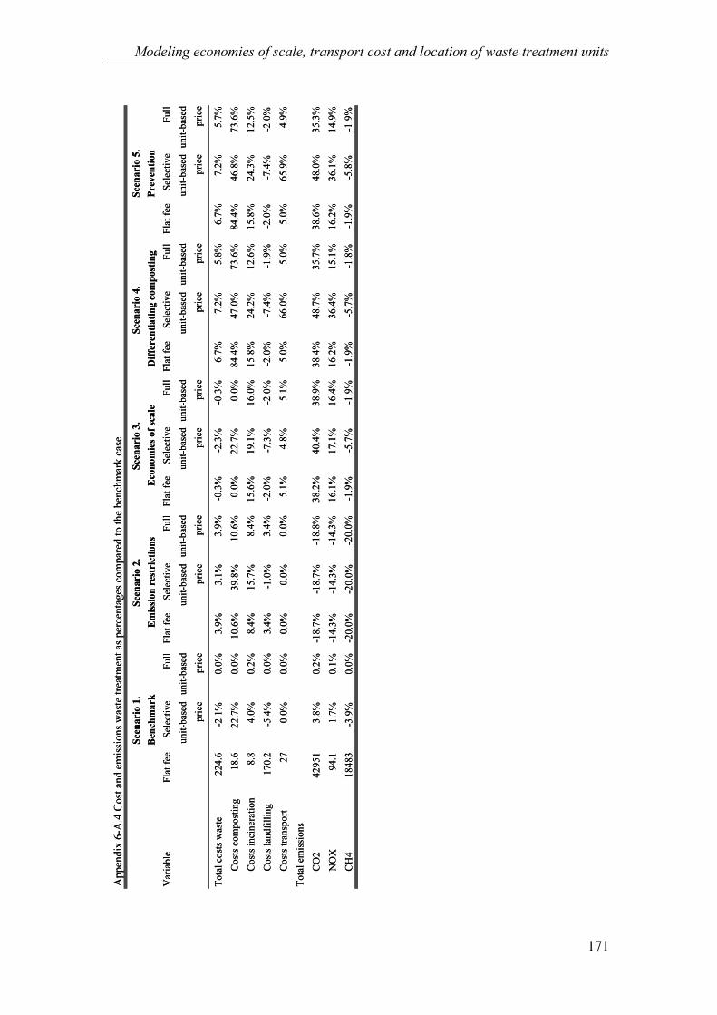
Modeling economies of scale, transport cost and location of waste treatment units
171
22
4.6
-2.1
%0
.0%
3.9
%3
.1%
3.9
%-0
.3%
-2.3
%-0
.3%
6.7
%7
.2%
5.8
%6
.7%
7.2
%5
.7%
Co
sts
com
po
stin
g1
8.6
22
.7%
0.0
%1
0.6
%3
9.8
%1
0.6
%0
.0%
22
.7%
0.0
%8
4.4
%4
7.0
%7
3.6
%8
4.4
%4
6.8
%7
3.6
%
Co
sts
inci
ner
atio
n8
.84
.0%
0.2
%8
.4%
15
.7%
8.4
%1
5.6
%1
9.1
%1
6.0
%1
5.8
%2
4.2
%1
2.6
%1
5.8
%2
4.3
%1
2.5
%
Co
sts
lan
dfi
llin
g1
70
.2-5
.4%
0.0
%3
.4%
-1.0
%3
.4%
-2.0
%-7
.3%
-2.0
%-2
.0%
-7.4
%-1
.9%
-2.0
%-7
.4%
-2.0
%
Co
sts
tran
spo
rt2
70
.0%
0.0
%0
.0%
0.0
%0
.0%
5.1
%4
.8%
5.1
%5
.0%
66
.0%
5.0
%5
.0%
65
.9%
4.9
%
CO
24
29
51
3.8
%0
.2%
-18
.7%
-18
.7%
-18
.8%
38
.2%
40
.4%
38
.9%
38
.4%
48
.7%
35
.7%
38
.6%
48
.0%
35
.3%
NO
X9
4.1
1.7
%0
.1%
-14
.3%
-14
.3%
-14
.3%
16
.1%
17
.1%
16
.4%
16
.2%
36
.4%
15
.1%
16
.2%
36
.1%
14
.9%
CH
41
84
83
-3.9
%0
.0%
-20
.0%
-20
.0%
-20
.0%
-1.9
%-5
.7%
-1.9
%-1
.9%
-5.7
%-1
.8%
-1.9
%-5
.8%
-1.9
%
Sel
ecti
ve
un
it-b
ased
pri
ce
Fla
t fe
e
Scen
ario
1.
Ben
chm
ark
Scen
ario
2.
Em
issi
on
res
tric
tio
ns
Sce
na
rio
3.
Eco
no
mie
s o
f sc
ale
Var
iab
leF
lat
fee
Sel
ecti
ve
un
it-b
ased
pri
ce
Fla
t fe
e
To
tal
emis
sio
ns
Appen
dix
6-A
.4 C
ost
and e
mis
sions
was
te t
reat
men
t as
per
centa
ges
com
par
ed t
o t
he
ben
chm
ark c
ase
Sel
ecti
ve
un
it-b
ased
pri
ce
Fla
t fe
eS
elec
tive
un
it-b
ased
pri
ce
Fla
t fe
eF
ull
un
it-b
ased
pri
ce
Fu
ll
un
it-b
ased
pri
ce
To
tal
cost
s w
aste
Sce
na
rio
5.
Fu
ll
un
it-b
ased
pri
ce
Fu
ll
un
it-b
ased
pri
ce
Fu
ll
un
it-b
ased
pri
ce
Sel
ecti
ve
un
it-b
ased
pri
ce
Pre
ven
tio
n
Sce
na
rio
4.
Dif
fere
nti
ati
ng
co
mp
ost
ing
22
4.6
-2.1
%0
.0%
3.9
%3
.1%
3.9
%-0
.3%
-2.3
%-0
.3%
6.7
%7
.2%
5.8
%6
.7%
7.2
%5
.7%
Co
sts
com
po
stin
g1
8.6
22
.7%
0.0
%1
0.6
%3
9.8
%1
0.6
%0
.0%
22
.7%
0.0
%8
4.4
%4
7.0
%7
3.6
%8
4.4
%4
6.8
%7
3.6
%
Co
sts
inci
ner
atio
n8
.84
.0%
0.2
%8
.4%
15
.7%
8.4
%1
5.6
%1
9.1
%1
6.0
%1
5.8
%2
4.2
%1
2.6
%1
5.8
%2
4.3
%1
2.5
%
Co
sts
lan
dfi
llin
g1
70
.2-5
.4%
0.0
%3
.4%
-1.0
%3
.4%
-2.0
%-7
.3%
-2.0
%-2
.0%
-7.4
%-1
.9%
-2.0
%-7
.4%
-2.0
%
Co
sts
tran
spo
rt2
70
.0%
0.0
%0
.0%
0.0
%0
.0%
5.1
%4
.8%
5.1
%5
.0%
66
.0%
5.0
%5
.0%
65
.9%
4.9
%
CO
24
29
51
3.8
%0
.2%
-18
.7%
-18
.7%
-18
.8%
38
.2%
40
.4%
38
.9%
38
.4%
48
.7%
35
.7%
38
.6%
48
.0%
35
.3%
NO
X9
4.1
1.7
%0
.1%
-14
.3%
-14
.3%
-14
.3%
16
.1%
17
.1%
16
.4%
16
.2%
36
.4%
15
.1%
16
.2%
36
.1%
14
.9%
CH
41
84
83
-3.9
%0
.0%
-20
.0%
-20
.0%
-20
.0%
-1.9
%-5
.7%
-1.9
%-1
.9%
-5.7
%-1
.8%
-1.9
%-5
.8%
-1.9
%
Sel
ecti
ve
un
it-b
ased
pri
ce
Fla
t fe
e
Scen
ario
1.
Ben
chm
ark
Scen
ario
2.
Em
issi
on
res
tric
tio
ns
Sce
na
rio
3.
Eco
no
mie
s o
f sc
ale
Var
iab
leF
lat
fee
Sel
ecti
ve
un
it-b
ased
pri
ce
Fla
t fe
e
To
tal
emis
sio
ns
Appen
dix
6-A
.4 C
ost
and e
mis
sions
was
te t
reat
men
t as
per
centa
ges
com
par
ed t
o t
he
ben
chm
ark c
ase
Sel
ecti
ve
un
it-b
ased
pri
ce
Fla
t fe
eS
elec
tive
un
it-b
ased
pri
ce
Fla
t fe
eF
ull
un
it-b
ased
pri
ce
Fu
ll
un
it-b
ased
pri
ce
To
tal
cost
s w
aste
Sce
na
rio
5.
Fu
ll
un
it-b
ased
pri
ce
Fu
ll
un
it-b
ased
pri
ce
Fu
ll
un
it-b
ased
pri
ce
Sel
ecti
ve
un
it-b
ased
pri
ce
Pre
ven
tio
n
Sce
na
rio
4.
Dif
fere
nti
ati
ng
co
mp
ost
ing

Chapter 6
172
Appendix 6-B Definition of indices, parameters, and variables
Indices
Label Range Description
c 1…2 traditional and green consumer
g 2 consumer goods
f 1...2 quality organic waste (low, high)
i 1...5 consumers
j 1...4 municipality
m 1..3 size waste treatment unit (small, medium, large)
s 1..3 type waste treatment units (composting, incineration, landfilling)
Parameters in GAMS specification
Symbol Description
α Negishi weight
β waste percentage
µ labor cost for generating organic waste
σk,l, substitution elasticity between labor and capital
σk,l,,e substitution elasticity between labor capital and emission rights
σl,h substitution elasticity between low and high quality organic waste
σ r,o substitution elasticity between rest waste and organic waste
σ m,s
substitution elasticity between landfilling and incineration
ξ subsidy wedge
A technology parameter waste treatment units
F flat fee for waste collection

Modeling economies of scale, transport cost and location of waste treatment units
173
K endowment of capital
L endowment of labor
LST lump sum transfer to keep income of government constant
p price
Pc price including subsidy
T total costs subsidy waste collection
Y0
initial income
Variables in GAMS specification
Symbol Description
e emission rights
k capital use
l labor use
q production
TWF total welfare
u utility
ts transport services
w generation of waste
wts waste treatment services
x consumption

Chapter 6
174

175
Part III
Conclusions and recommendations

176

177
7 Summary, conclusions and recommendations
7.1 Introduction
Each year the Netherlands spends approximately 3.5 billion Euros on the treatment of
waste. Waste treatment not only costs our society a lot of money, but it also creates
environment problems. For example, the landfilling of waste generates about 40% of
total methane emissions in the Netherlands. The Dutch government is, therefore, very
eager to reduce waste generation as much as possible. Annually, households and
industry generate about 12 Mtonnes of waste. Although this is still a considerable
amount of waste, the quantity of waste generated today is already 40% lower than the
quantity generated in 1990. In particular, the industrial sector and the construction and
demolition sector have started to recycle far more waste as compared to 1990. These
sectors recycle about 90% of all their waste, which naturally results in far less waste
incinerated or landfilled. Private households do not recycle nearly as much. On
average, only about 40% of all municipal solid waste is recycled. The amount of solid
waste generated increases every year due to economic growth; though thus far it has
not been possible to decouple economic growth and the generation of municipal solid
waste.
Although the Dutch government has tried to stimulate waste separation and recycling
since the beginning of the 1990s, the results are not promising. Since 1995, for
example, municipalities have been obliged to collect organic waste separately from
rest waste. Despite the initial increase of organic waste collected in 1995, since that
time the amount of organic waste generated has hardly increased at all. Annually,
about 12% of all municipal solid waste is collected as organic waste and composted.
This, however, does not necessarily mean that all organic waste is collected
separately. On average, about 34% of the waste collected as rest waste is actually
organic waste. If households separated all organic waste from rest waste, a significant
saving on the expenses of waste treatment, about 170 million Euros, could be made.
The incineration of rest waste is namely twice as expensive as the composting of
organic waste.
The failure to increase recycling and waste separation has been caused by a number of
distortions in the municipal solid waste market. It is important to analyze how these
market distortions can be resolved. Only if these distortions are resolved, will it be
possible to reduce waste generation, and thus the social costs of waste treatment also.
For this reason, this thesis has aimed to analyze the municipal solid waste market in
the Netherlands. The main objectives, as formulated in Chapter 1, were: (1) To

Chapter 7
178
analyze how the incentive structure of the consumers, emission restrictions,
interrelations between the municipal solid waste sector and the rest of the economy
and the spatial aspects of the waste problem influence the optimal municipal solid
waste management plan. (2) To asses whether a flat fee-pricing system, a unit-based
pricing system for the collection of rest waste, a unit-based pricing system for the
collection of organic and rest waste, or a recycling subsidy is the preferable policy
option to minimize the social costs of municipal solid waste treatment. (3) To gain
insight into how to develop a more efficient municipal solid waste management plan,
which solves inefficiencies caused by market distortions present in the municipal solid
waste market.
On the basis of these objectives, five research questions were formulated in Chapter 1.
In this chapter, the most important results of the thesis will be presented by answering
these research questions.
7.2 The economic and environmental topics concerning the
municipal solid waste management problem
Research question 1:
What are the most important environmental and economic topics with regard to the
municipal solid waste management problem?
Besides financial costs, waste treatment also creates many environment problems. As
policy makers are concerned about the state of the environment, they have adopted the
concept of the waste hierarchy as a basis for waste policies. The waste hierarchy is a
method to prioritize different waste handling options. According to the waste
hierarchy, the prevention of waste has the absolute preference, followed by recycling
and re-use, composting, incineration and, as the last option, landfilling.
Since landfilling is the least preferred waste treatment method, the government has
tried to prevent the landfilling of waste as much as possible. For this reason, two
policy measures were introduced, namely a ban on landfilling and a landfilling tax. As
a result, landfilling of waste decreased dramatically. In 2002, for example, 5157
Ktonnes of waste were landfilled; compared to 1992 this meant a decrease of more
than 60%. Increasingly less waste has thus been landfilled and increasingly more
waste recycled, composted, or incinerated. In this way, the government has tried to
control waste flows in an environmentally sound manner and minimize social waste
treatment costs. Although it may seem that the landfilling tax has been rendered
obsolete by the ban on landfilling, the landfilling tax is still necessary to control the
waste flows. Producers were often granted an exemption from the ban on landfilling,
because the incineration capacity in the Netherlands was not large enough to

Summary, conclusions and recommendations
179
incinerate all combustible waste. Producers were very keen on getting such an
exemption, since landfilling was far cheaper than incineration or recycling. The
introduction of a landfilling tax, which raised the price of landfilling above the price
of incineration, provided the necessary price-incentive to the production sectors to
recycle or incinerate their waste as much as possible.
Although it serves a useful purpose, the waste hierarchy should not be considered the
only rule that may determine the optimal waste treatment option. It is important to
bear in mind that, in some cases, a strict application of the waste hierarchy can do our
society more harm than good. Each waste handling option, i.e. recycling, re-use,
composting, incineration, or landfilling, may lead to environmental damage. Since
each waste treatment unit is unique and operates quite differently to the others, is it
important to realize that one waste treatment unit will process waste in a more
environmental friendly way than another. Large waste treatment units, for example,
have more capital to invest in emission reduction measures than smaller installations.
For this reason, is it important to include economies of scale in the analysis in order to
determine the socially most efficiently waste management plan.
The minimization of social waste treatment costs is not the only solution to the waste
management problem, it is also important to minimize the amount of waste generated.
The production sectors have a strong financial incentive to decrease their generation
of waste due to a significant landfilling tax. The treatment of waste has become
expensive and thus the production sectors have increasingly invested more in
advanced recycling technologies.
The municipal solid waste problem is much more difficult to control. In most cases,
households pay a flat fee for the collection of waste. This flat fee is not related to the
amount of waste that is generated and collected. Thus, an increase in the cost of waste
treatment has no or only a negligible effect on the generation of municipal solid
waste. In addition, the municipal solid waste stream is very diverse. Municipal solid
waste consists of several different waste materials. This makes it difficult to recycle
waste to a large extent.
Due to the presence of market distortions in the municipal solid waste market, waste
treatment costs are higher than desirable. Based on recent literature as described in
Chapter 2, three market distortions can be distinguished: (1) the flat fee (2) indirect
subsidizations of the use of raw materials and (3) ‘killer contracts’ between waste
treatment facilities and municipalities that specify the quantity of waste the
municipalities must deliver to the facilities and the price they will have to pay to
dispose of this waste.
Chapter 2 provides an overview of the recent literature, which analyses possible
solutions to these market distortions. From the literature, it may be concluded that

Chapter 7
180
particularly the flat fee has significant consequences for the total generation of
municipal solid waste. Therefore, the flat fee must be replaced by another pricing
system. A possible replacement of the flat fee is a unit-based price for waste
collection. The unit-based price will decrease waste generation. However, given that
unit-based pricing can stimulate illegal disposal, it is important that the prevention of
illegal dumping of waste is given special attention.
Recent studies, such as Palmer and Walls (1997), Fullerton and Kinnaman (1998), and
Walls and Palmer (2000), have neglected several important aspects of the municipal
solid waste market, thus their analyses of the effects of introducing unit-based pricing
for waste collection are incomplete. First of all, the phenomenon ‘waste leakage’ has
been left out of the analysis. Consumers determine the quality of waste they generate.
They can choose to generate rest waste that is ‘polluted’ with, for instance, organic
waste, glass, or paper. This has no direct consequence for the treatment costs of waste
as experienced by the individual consumer, as organic waste, or paper can be
incinerated without any problems. It is, however, lamentable that paper, and organic
waste are not recycled or composted, since recycling and composting are much
cheaper and generate less environment pollution than incineration. It is also possible
that consumers pollute glass, paper, or organic waste with rest waste. This has more
serious consequences. Polluted glass and paper must first be cleaned before it can be
recycled. Heavily polluted organic waste will be rejected by the composting unit,
which means that this polluted organic waste must be incinerated. A composting unit
cannot compost polluted organic waste, because the quality of compost produced
from polluted organic waste is not good enough to sell1. The introduction of a unit-
based price for waste collection may increase this kind of undesirable pollution of
waste and it is therefore crucial that the possibility of ‘waste leakage’ be included in
the analysis.
Secondly, an analysis of the spatial aspects of the waste problem within a general
equilibrium framework is missing in the literature. The costs of waste treatment are
significantly influenced by the location of the waste treatment unit, the transport costs
and economies of scale of the waste treatment units in question. These costs also
depend on the quantity as well on the quality of the waste generated. A change in the
composition of the waste stream, due to the introduction of a new policy measure, can
have significant consequences for both the optimal location of the waste treatment
facility and waste treatment costs. The waste treatment costs may in turn significantly
influence the amount of municipal solid waste generated. It is important that these
1 Even if polluted organic waste is cleaned, the amount of heavy metals in the organic waste will be so
high that it is impossible to produce high quality compost from the waste.

Summary, conclusions and recommendations
181
interactions between the spatial aspects of waste treatment and waste generation be
included in the analysis.
To summarize, the economic and environment issues in relation to the waste
management problem can be divided into two areas of interest. Firstly, the problem of
how waste should be treated so that the costs to society are as low as possible must be
solved. Waste treatment generates both financial and environmental costs. Since the
environmental costs are not internalized in the price of waste treatment and thus the
social waste treatment costs are higher than optimal, the Dutch government has
adopted the concept of waste hierarchy as the basis for an optimal waste management
plan. Scientific research has warned that a strict regime, such as the waste hierarchy,
can lead to more waste treatment costs than necessary. The existing literature
demonstrates that it is more appropriate for the choice between waste treatment
options to be determined on an individual case basis. Secondly, the problem of how to
minimize waste generation should be answered. In the Netherlands, consumers
generate most of the waste to be treated, i.e. organic waste and rest waste. The present
structure of the municipal solid waste market leads to an inefficient high quantity of
waste. Policy tools, such as a differentiated price for waste collection, a recycling
subsidy, or an advanced disposal fee, which internalizes the costs of waste treatment
in the price of a product, could be used to decrease waste generation.
In this thesis, these waste management issues have been linked. The optimal waste
treatment method and the minimization of waste treatment costs are thus coupled. The
quality and quantity of municipal solid waste influence the treatment of the waste. For
example, high quality organic waste may be composted, but low quality organic waste
can only be incinerated or landfilled. Moreover, the treatment costs can influence the
amount of municipal solid waste generated. In an undistorted market, for example,
higher treatment costs result in the generation of less waste.
7.3 The problems concerning the flat fee for waste collection
Research question 2:
How does the market distortion caused by the flat fee-pricing system influence
municipal solid waste generation and how can these negative effects be sufficiently
reduced?
Most municipalities in the Netherlands charge a fixed amount of money, the so-called
flat fee for collection of waste. Although this amount is determined on the basis of the
household size, the amount is independent from the actual quantity of waste
generated. Households have no financial incentive to decrease waste generation.
Empirical studies show that the introduction of a unit-based price for waste collection,

Chapter 7
182
the so-called unit-based price, can have a strong influence on the quantity of waste
generated. In those municipalities that introduced a unit-based price, the quantity of
rest waste declined by about 20 to 30% (KPMG, 1999). However, the extent to which
this reduction may be attributed to the introduction of a unit-based price is unclear.
Thus far, the introduction of a unit-based price in the Netherlands has always been
combined with programs to stimulate both recycling and prevention of waste.
Therefore, recycling programs may be responsible for part of the observed reduction.
Theoretical studies warn that price-differentiation may lead to the illegal dumping of
waste, but up until now there has been little empirical proof to support this assertion.
Municipalities may choose between different forms of price differentiation. The
possibilities are price differentiation on the basis of volume, weight, or frequency of
collection or a combination of these forms. It is also possible to sell special waste
bags, in which the consumers have dispose of their waste; this system is called price
differentiation on the basis of an ‘expensive bag’. Each of these unit-based pricing
schemes has advantages and disadvantages, but the greatest advantage of each of
these schemes is that they decrease the generation of municipal solid waste. In this
thesis, I have shown, with the use of a general equilibrium model, that the flat fee
indeed results in inefficiently high waste generation, just as empirical studies have
shown.
Chapter 4 deals with a comparison between four policy instruments: 1) the
introduction of a recycling subsidy combined with a flat fee, 2) the introduction of a
unit-based price for waste collection, 3) the introduction of a recycling subsidy
combined with an unit-based price and 4) an advanced disposal fee on the price of a
consumption good.
The results show that a flat fee distorts the municipal solid waste market. The
introduction of an incentive to increase recycling, by means of a recycling subsidy,
has no significant effect, since consumers are given no incentive to reduce their
generation of rest waste. Although recycling becomes cheaper due to the recycling
subsidy, the collection of rest waste is free of charge, which therefore means that
consumers do not invest in efforts to increase recycling. The introduction of unit-
based pricing in the model has more effect on waste generation and recycling. The
quantity of rest waste generated decreases by about 2% and recycling increases by
about 6%. If the introduction of unit-based pricing is combined with the introduction
of a recycling subsidy, the effects are even more impressive. Rest waste decreases by
about 70% and recycling increases by about 266%. It should be noted that no
technical upper boundary is placed on the quantity of waste that can be recycled, in
reality this is not possible, and therefore the model may overestimate the effect of the
policy instrument. The advanced disposal fee on the price of consumption goods also
decreases waste generation, but to a lesser extent. Waste generation decreases by

Summary, conclusions and recommendations
183
0.5% when an advanced disposal fee, which covers the actual waste treatment costs, is
introduced. The advanced disposal fee, in contrast to a unit-based price, stimulates
waste prevention but not recycling. Thus this policy instrument only has a limited
impact on waste generation.
Considering the results of this model, the introduction of unit-based pricing is the
most effective method for decreasing waste generation, especially if combined with a
recycling subsidy. The introduction of an advanced disposal fee is much less efficient.
Although it stimulates prevention, the reduction of rest waste generated is rather
small. The advanced disposal fee is not as effective as the unit-based pricing scheme
because: firstly, the advanced disposal fee is too low to change consumption patterns
significantly2 and secondly, the waste collection fee does not stimulate recycling since
consumers no longer have to pay a fee for the actual collection of waste. They only
pay a fee for collection and treatment of waste while buying the product, thus they do
not have a price-incentive to recycle.
The model, presented in Chapter 4, does not include the possible evasive behavior of
consumers. Consumers can easily reduce the quantity of rest waste they generate by
disposing of it in the organic waste bin. Moreover, the link between generation of
waste and treatment of waste, which was discussed in Section 7.2, is not included in
this model. The following two research questions will deal with the question of how
these two issues influence the effectiveness of unit-based pricing.
7.4 The problems of waste leakage
Research question 3:
How great a problem is waste leakage and how is waste leakage influenced by
household attitudes?
Municipalities can introduce unit-based pricing for all waste streams or only for a
single waste stream. In practice, unit-based pricing has been introduced for the
collection of rest waste and/or organic waste. Recyclable waste, such as glass and
paper, is collected free of charge. Whether one should introduce unit-based pricing for
the collection of organic waste is not an easy question to answer. If a municipality
wants to stimulate separation of waste, it is undesirable to charge an equal price for
the collection of organic and rest waste. As the separation of waste requires extra
2 The advanced disposal fee internalizes the costs of waste treatment in the price of the consumer good.
As the disposal costs of a good are generally much lower than the production costs of the good,
consumers have only a very small incentive to change their consumption patterns.

Chapter 7
184
effort on the part of consumers, it should be stimulated by a price-incentive.
Moreover, the treatment of organic waste is far less costly than the treatment of rest
waste and, therefore, it is difficult to explain to the consumers that the price of
collecting organic waste is equal to the price of collecting rest waste. If municipalities
charge the same price, they can lose a lot of goodwill, possibly resulting in a situation
where consumers are unwilling to put extra effort into waste separation and are more
inclined to dispose of waste in an illegal manner.
Waste leakage is one of the possible options consumers have to dispose of rest waste.
In this case, consumers throw rest waste away with organic or recyclable waste and
thus pollute these waste streams. Households need not to be afraid of being penalized
for this undesirable behavior. It is, for example, very expensive to check the quality of
the organic waste during collection. The quality of the waste is instead checked at the
composting unit. At this point, it is extremely difficult to determine exactly which
household has polluted the waste stream. The only option a municipality has in such a
case is to appeal to the whole district about the quality of the waste the district has
supplied.
In this thesis, I have developed a general equilibrium model to study the problems
caused by waste leakage. In Chapter 5, I demonstrate how the effects of waste leakage
can be a serious impediment to the introduction of unit-based pricing for the
collection of municipal solid waste. The analysis is restricted to the introduction of
weight-based pricing for waste collection, but a similar analysis may be made for the
introduction of price differentiation on the basis of collection frequency or volume.
This only affects the method according to which waste generation is calculated in the
model.
The analysis in Chapter 5 shows that consumers start to pollute organic waste due to
the introduction of unit-based pricing for collection of rest waste. After the
introduction of unit-based pricing, consumers generate about 10% less rest waste.
Consumers reduce their generation of rest waste by substituting it for low quality as
well as high quality organic waste. High quality organic waste consists of 100%
organic waste. Low quality organic waste consists of 70% organic waste and 30% rest
waste (non-organic residue). On average, after the introduction of price differentiation
consumers generate about 46% more low quality and 22% more high quality organic
waste. This means that the percentage of rest waste thrown away with organic waste
increases from 5.5% to 6.7%.
Not every household reacts in the same way to the introduction of price
differentiation. Depending on the preferences of the consumers, they will be inclined
to behave in a more or lesser environment friendly fashion. A ‘traditional’ consumer
has little interest in the environment and will be more inclined to pollute waste than a
‘green’ consumer, who cares for the state of the environment. Model results in

Summary, conclusions and recommendations
185
Chapter 5 demonstrated that ‘green’ consumers generate about 14% less rest waste
when unit-based pricing is introduced. They will approximately generate 14% more
low quality organic waste and 12% more high quality organic waste. The percentage
rest waste that is thrown away with organic waste remains constant, about 3.1%. The
‘traditional’ consumers generate 8% less rest waste. They generate approximately
63% more low quality organic waste and 41% more high quality organic waste. This
means that the percentage of rest waste thrown away with organic waste increases
from 9.8% to 11%.
Although the overall percentage of rest waste thrown away with organic waste, i.e. by
both ‘green’ and ‘traditional’ consumers, does not increase significantly, i.e. from
5.5% to 6.7%, it is important to bear in mind that this is an average percentage. Waste
is collected in relative small quantities; approximately 28 tonnes of waste fit in one
garbage truck. Some districts in a municipality may be house comparatively more
‘green’ consumers, while other districts may house proportionally more ‘traditional
consumers’. In a district with many ‘traditional’ consumers, the quality of organic
waste collected will decline far more than in districts with a lot of ‘green’ consumers.
This can mean that the organic waste collected in these districts cannot be composted.
IPH (1995) shows that composting units will in general reject organic waste of such
low quality as generated by the ‘traditional’ consumers.
The introduction of unit-based pricing will lead to the situation where waste collected
in some districts is rejected by composting units. Particularly in large cities with a
high percentage of ‘traditional’ consumers, the organic waste will be heavily polluted.
When municipalities consider introducing unit-based pricing, it is important that they
bear in mind that waste leakage may occur. Large cities can only consider unit-based
pricing in those districts where relatively many ‘green’ consumers live. Such a kind of
selective regulation is used more often: for instance, it has already been introduced in
large cities, as Utrecht and Amsterdam. In these cities, organic waste and rest waste
are collected separately only in a restricted number of districts. In the other districts,
the quality of the organic waste was found to be too low to compost and thus could
not justify the additional collecting cost.
A possible solution for the problem of waste leakage is the introduction of a unit-
based pricing for rest waste as well as organic waste. Since consumers pay the same
price for collection of both rest and organic waste, they have no incentive to pollute
organic waste. As was already observed in the introduction to this section, the danger
of such a system is that the goodwill of the consumer may be compromised. This is
illustrated by the quantitative results of Chapter 6. If unit-based pricing for the
collection of rest waste as well as organic waste is introduced, consumers do not start
to generate more organic waste. The ‘traditional’ consumers even generate more low
quality organic waste and less high quality organic waste. Only if it is possible to

Chapter 7
186
increase the price of collection of low quality organic waste as compared to the price
of collection of high quality organic waste, does unit-based pricing result in a
decrease of the generation of low quality organic waste.
7.5 Choice of the optimal location of waste treatment units
Research question 4:
How is the choice of the optimal location of waste treatment facilities influenced by
the quantity and quality of municipal solid waste generated by consumers and,
moreover, how will the spatial aspects of the municipal solid waste management
problem in turn influence the successfulness of introducing unit-based pricing?
In principle, municipalities determine how waste is treated and at which location.
Municipalities are, however, not completely free in this choice. Depending on the type
of waste collected, they will decide how to process the waste. The collected organic
waste will always go to a composting facility. The collected rest waste is sent to either
an incineration plant or a landfill site. The quantity of waste collected influences the
optimal waste treatment method and location. Due to economies of scale in waste
treatment, large quantities of waste can be processed more cheaply than small
quantities. Economies of scale play a particularly important role in the case of
incineration, also due to environment regulations that specify the extent of emissions
permitted. Thus, it is much cheaper for a municipality to allow waste to be treated in a
large waste treatment unit than in a small one, although this will increase transport
costs.
The introduction of unit-based pricing alters the composition of the collected
municipal solid waste stream. Municipalities collect less rest waste, and more organic
waste. The quantitative results of Chapter 6 show that if unit-based pricing for the
collection of rest waste is introduced that municipalities will collect about 6% less rest
waste. If a unit-based price for the collection of rest waste as well as organic waste is
introduced, the total quantity of organic waste and rest waste remains constant.
The change in composition of the municipal solid waste stream has significant
consequences for the optimal location choice of waste treatment units. If more organic
waste is collected, it is attractive for organic waste to be treated in a large composting
unit. If the quality of organic waste declines sharply, it is also attractive to treat waste
at lower costs.
The analysis in Chapter 6 demonstrates that the quality of the organic waste in large
cities declines significantly due tot the introduction of unit-based pricing. As a result,
these municipalities treat their waste in large composting units. This means that

Summary, conclusions and recommendations
187
transport costs increase significantly, about 60%. As a result, the total costs of waste
treatment increase slightly after the introduction of unit-based pricing, from 239.6
million Euros to 240.7 million Euros.
Since municipalities have negotiated contracts with incineration plants, composting
units and landfill sites, it is not possible to switch from one installation to another in
the short term. This does not, however, mean that the effects of changes in the
composition of the municipal solid waste stream due to the introduction of unit-based
pricing should be disregarded. By introducing unit-based pricing, the composition of
the municipal solid waste stream permanently changes. In the long run, municipalities
are not bound by contracts with waste treatment units and they can switch between
these waste treatment units.
The results in Chapter 6 show that the environment effects due to the introduction of
unit-based pricing are ambiguous. If unit-based pricing is introduced less rest waste
will be generated. This means that less rest waste will have to be incinerated or
landfilled, resulting in a decrease of both CO2 and CH4 emissions. Although more
organic waste is generated, part of it is of such low quality that it has to be
incinerated, resulting in an increase of CO2 emissions. Moreover the transport of
waste increases, which generates more NOX emissions. The net effects are an increase
of CO2 emission by 6.8% and an increase of NOX emissions by 17%. CH4 emissions
decrease by 4%.
It may be clear that there is a strong interaction between quality of waste and
treatment of waste. Although unit-based pricing leads to a decrease in the amount of
rest waste generated, the costs of waste treatment do not decline. The results in
Chapter 6 illustrate that waste leakage influences the optimal treatment option so that
municipalities will switch from small composting units to large ones, thus increasing
transport costs. Chapter 6 also shows that the introduction of unit-based pricing is
only attractive in small municipalities with proportionally more ‘green’ consumers.
For larger cities, the consequences of waste leakage are too far-reaching to justify the
costs of introducing unit-based pricing.
7.6 Policy recommendations
Research question 5:
Which kinds of policy changes can be recommended to minimize the total social costs
of municipal solid waste treatment for our society?

Chapter 7
188
In this thesis four policy options have been analyzed, namely 1) a flat fee, 2) a
recycling subsidy, 3) a unit-based price for collection of rest waste and 4) a unit-based
price for collection of rest waste as well as organic waste.
As mentioned above, most municipalities in the Netherlands charge a flat fee for the
collection of municipal solid waste. If a flat fee is charged, consumers have no
incentive to separate or recycle waste, thus consumers generate more waste than is
social desirable. The main advantage of the flat fee-pricing scheme is the low
collection cost, since municipalities do not have to keep track of the quantity of waste
generated by an individual household. Another advantage is that consumers have no
incentive to illegally dump their waste or to pollute the recyclable or organic waste
stream.
To promote recycling, the municipality can choose to subsidize it. Recycled material
is on average more expensive than virgin material; this makes recycled material
difficult to sell. By subsidizing the recycling process, the government can stimulate
the use of recycled materials. If, however, a recycling subsidy is combined with a flat
fee for waste collection, then the introduction of a recycling subsidy will have little
effect. The flat fee distorts the municipal solid waste market, for consumers have no
price incentive to reduce the generation of rest waste. Unless additional incentives are
provided, they will not recycle more, as this is costly for the consumers, not even if it
is deemed socially very desirable. For this reason, it is not advisable to for a recycling
subsidy to be introduced without accompanying measures, if the municipality in
question also charges a flat fee for waste collection.
If a recycling subsidy is jointly implemented with a unit-based pricing scheme, then
the recycling subsidy has a positive effect. More waste will be recycled and less virgin
materials will be used. This effect, although to a lesser extent, will also be
accomplished through the introduction of unit-based pricing without a recycling
subsidy. Municipalities may consequently introduce unit-based pricing and leave the
use of recycled material with respect to virgin materials up to the market.
By introducing unit-based pricing, municipalities can stimulate recycling and waste
separation. Due to the introduction of unit-based pricing, consumers are given a price
incentive to decrease the generation of rest waste. Unit-based pricing on basis of
weight is especially effective in reducing the generation of rest waste. This greatly
decreases the money spent on the incineration and landfilling of waste.
Municipalities can choose whether to introduce unit-based pricing for rest waste, or
for rest waste as well as organic waste. If they introduce unit-based pricing for rest
waste as well as organic waste, the consumers will not be stimulated to put extra
effort into the separation of organic and rest waste. Having to separate waste may also
diminish the goodwill of consumers. The consumers have to invest a lot time and

Summary, conclusions and recommendations
189
energy in separating rest waste and organic waste. When consumers are not
financially compensated for such efforts, they may be inclined to stop separating
waste partly or altogether. If they are forced to pay the same amount for the collection
of organic waste and rest waste, their resistance will be even greater. Organic waste is
much cheaper to process than rest waste and the marginal costs of treating organic
waste are less than the marginal costs of treating rest waste. Therefore, by demanding
an equal price for the collection of both organic and rest waste, the consumers are
more or less financially penalized for waste separation.
The introduction of unit-based pricing for the collection of rest waste stimulates
consumers to generate less rest waste. They can accomplish this by separating organic
waste from rest waste or by preventing waste generation. A major disadvantage of this
policy instrument is the possibility of waste leakage. If organic waste is heavily
polluted by rest waste, it can no longer be composted. In this case, the polluted waste
will have to be incinerated, thus leading to significantly higher waste treatment costs.
To summarize, the question of which policy option can be recommended cannot be
answered unequivocally. The introduction of a recycling subsidy is not recommended,
since the municipal solid waste market is distorted due to the flat fee for waste
collection; a recycling subsidy will, therefore, have no effect on the recycling
behavior of consumers. If the government wants to stimulate recycling, the
introduction of unit-based pricing for waste collection will be more effective. Unit-
based pricing for the collection of rest waste provides the greatest incentive for waste
separation, but also provides the prime incentive for waste leakage. In smaller
municipalities, the introduction of price differentiation for both organic waste and rest
waste is possible. In smaller municipalities with proportionally more ‘green’
consumers, it is also possible to introduce price differentiation for rest waste only.
With the help of a numerical analysis, in Chapter 6 I have shown that the danger of
waste leakage is not so great in these small municipalities and therefore the benefits of
introducing price differentiation outweigh the costs. Municipalities with
proportionally more ‘traditional’ consumers should be aware of problems created by
waste leakage. In these municipalities, unit-based pricing for rest waste as well as
organic waste performs far better. In larger municipalities, only the introduction of
unit-based pricing for rest waste as well as organic waste is advisable. Due to the
problems caused by waste leakage, the introduction unit-based pricing for rest waste
alone is not attractive.
If the problems created by waste leakage can be solved, unit-based pricing is certainly
an attractive policy instrument. Unit-based pricing is the only policy instrument that
can potentially stimulate prevention, recycling, and waste separation simultaneously.
Pollution of the recyclable waste steam, like glass and paper, is expensive, but not as
problematic as the pollution of the organic waste stream. Heavily polluted recyclable

Chapter 7
190
waste can be cleaned and then recycled, whereas heavily polluted organic waste
cannot be composted even if it is cleaned.
It is possible to clean polluted organic waste, consider, for example, the cleaning
techniques employed by the VAGRAM installation in Groningen, but the quality of
the compost produced from polluted organic waste is not good enough to sell. It is
important that the government stimulates the development of better separation and
cleaning techniques, because the introduction of unit-based pricing is an important
means to minimize the generation of municipal solid waste and to increase recycling
percentages.
7.7 Modeling of the waste problem
In addition to the above research questions, the following three modeling questions
were formulated in Chapter 1:
• How can interactions between the waste sector, government policies, and the rest
of the economy be modeled?
• How can the flat fee-pricing system be introduced to a general equilibrium
setting?
• How can spatial aspects of the waste management problem, such as a fixed set of
possible location of waste treatment centers, economies of scale and transport
costs, be introduced to a general equilibrium framework?
In this thesis, I have demonstrated how the different aspects of the waste problem, as
formulated in the model questions, can be implemented in a general equilibrium
framework. In particular, it was difficult to incorporate the flat fee into a general
equilibrium model.
By using the subsidy-cum-tax system, the problem of a marginal zero price for waste
collection can be avoided. In this system, consumers pay an equilibrium price for
collection of waste. The government reimburses consumers with a subsidy that covers
the exact price of waste collection. Thus, the price of waste collection, as perceived by
the consumers, equals zero. The consumer pays a direct tax for the collection of the
waste to the government, the so-called flat fee. In sum, in this system consumers pay a
direct tax for waste collection, but this tax is not related to the quantity of waste they
generate.
In Chapters 4, 5 and 6, three different general equilibrium models have been
developed. All these models were built in the Negishi format. The models have been

Summary, conclusions and recommendations
191
constructed from a relatively simple (Chapter 4) to a detailed and complex analysis of
the waste problem (Chapter 6).
To summarize, the most complex model developed in Chapter 6 had the following
characteristics:
1) The economy is divided in four municipalities. Within a municipality, two
types of consumers are distinguished: a ‘green’ consumer and a ‘traditional’
consumer. The ‘green’ consumer is more environment friendly oriented than
the ‘traditional’ consumer. The municipalities differ in the share of ‘green’ and
‘traditional’ consumers.
2) Municipalities can treat waste in composting units, incineration plants, and
landfill sites. Three sizes are distinguished for each waste treatment unit: a
small-sized, a medium-sized and a large-sized unit. Economies of scale
influence waste treatment costs; a large installation treats waste for a lower
price than a small installation. Apart from waste treatment costs,
municipalities also face transport costs. As large installations are, on average,
located further away from the municipalities, transport costs are higher for
these waste treatment units.
3) Policy measures, such as emission reductions, flat fees and unit-based pricing,
can be included in the model without any problems.
The models presented in this thesis make it possible to analyze the effects of
introducing price differentiation. New to the analysis is the explicit modeling of the
quality of waste, the possibility of waste leakage, the link between production of
municipal solid waste, the collection of waste by municipalities, and the treatment of
waste by waste treatment units and finally the modeling of spatial aspects of waste
treatment within a general equilibrium framework.
In contrast to the existing literature, in this thesis a link is made between the
generation and treatment of waste. Thus, a detailed analysis of the cost-effectiveness
of the introduction of unit-based pricing could be made. In this thesis, I demonstrated
that a decrease of the quality of waste, due to the introduction of unit-based pricing,
has a significant effect on the costs of waste treatment and thus on the cost-
effectiveness of unit-based pricing also.
By using a general equilibrium framework, it was possible to analyze these relations
in detail. A general equilibrium model describes all relevant markets in the economy,
calculates the interactions between the different markets, and forms a closed system.
The results of the models suggest that the success of unit-based pricing to a large
extent depends on the preferences of the consumers. In those districts, in which

Chapter 7
192
proportionally more ‘traditional’ consumers live, unit-based pricing will not be
successful.
By modeling both the consumption and the production sector, I was able to show that,
against expectations, unit-based pricing alone is not suitable for stimulating
prevention. The price incentive in the waste sector is too small to significantly change
consumption patterns. If the government wants to stimulate prevention, they will have
to consider other policy measures.
As demonstrated in this thesis, the preferences of the consumers, the location and the
economies of scale play an important role in determining the optimal waste
management policy. This means that a national waste management plan for municipal
solid waste can only be successfully designed if specific local circumstances are
explicitly considered. The success of unit-based pricing will depend on the share of
‘green’ and ‘traditional’ consumers living in the municipality, or living in a district of
the municipality. Thus, each municipality will have to decide for itself whether unit-
based pricing will be a success or not.
7.8 General conclusions
To summarize, this thesis has contributed to our understanding of the impact of the
introduction of unit-based pricing.
1) Unit-based pricing will be successful in some municipalities, but not in all due
to the possibility of waste leakage. All municipalities will have to accept that
some amount of waste leakage occurs, but municipalities with proportionally
more ‘green’ consumers will have a lower increase of waste leakage and thus
the costs-effectiveness of unit-based pricing is greater in these municipalities.
Each municipality should analyze for itself whether the introduction of unit-
based pricing is cost-effective. A national waste management plan for
municipal solid waste that does not consider the specific characteristics of
municipalities and households will therefore be less than optimal.
2) Unit-based pricing is not suitable for stimulating prevention. The results of
this thesis demonstrate that a policy change in the waste sector is not sufficient
to shift consumption patterns. Unit-based pricing, however, is suitable to solve
the market distortion caused by a flat fee pricing system. If unit-based pricing
is introduced, other policy tools, such as a recycling subsidy, are more
effective. If, for example, a recycling subsidy was to be implemented in
combination with a flat fee for waste collection, the recycling subsidy would
not stimulate recycling due to the market distortions created by the flat fee-
pricing scheme.

Summary, conclusions and recommendations
193
3) The impact of the quality and quantity of waste on the costs of waste treatment
can be analyzed by explicit modeling of the link between waste generation and
waste treatment, thus a more detailed analysis about the cost-effectiveness of
unit-based pricing can be made. This thesis shows that the introduction of unit-
based pricing is by no means as beneficial for the environment as expected on
the basis of the reduction of waste generation. Unit-based pricing decreases
generation of rest waste, but also decreases the quality of organic waste.
Consumers not only start to separate more organic waste from rest waste, but
also pollute more organic waste with rest waste. Due to this waste leakage
effect, the costs of composting, the transport costs, and the corresponding
emission costs also increase.
7.9 Research recommendations
In this thesis, a model to analyze the effects of waste leakage has been developed. The
model calculates the impact unit-based pricing has on the quality of organic waste and
the subsequent costs of waste treatment. In this model, I have included three types of
emissions, two types of consumers, four municipalities, transport costs, economies of
scale and differentiated prices for composting high and low quality organic waste. The
model is used in a stylized example with numerical data based on the ‘Randstad’ in
2000.
The most complex model, as described in Chapter 6, incorporates a large number of
aspects of the waste market in the analysis. However, some more aspects could be
added to the model to predict the effects of unit-based pricing with greater certainty.
Firstly, the model could be expanded to include several waste streams. In this thesis, I
have concentrated on organic waste and rest waste. Other recyclable waste streams,
like glass, paper, and aluminum, could also be included in the analysis.
Secondly, it would be interesting to include home composting as well as illegal
dumping in the model. The first option provides consumers with a legal option to
decrease organic waste generation; home composting on large scale can, however,
lead to problems for the composting industry. The second option provides consumers
with an illegal option for getting rid of rest waste. This option will, of course, increase
the social costs of waste treatment and can be a serious impediment to the
introduction of unit-based pricing.
Thirdly, it is important to examine how prevention can play a role in solving the waste
management problem in greater detail. Although I considered prevention as an option
in this thesis, prevention was modeled rather simplistically. In the model in Chapter 6,
only two consumer goods were included, i.e. a consumption good with a large waste
Chapter 7
194
content and a consumption good with a small waste content. Consumers could
influence waste generation by consuming less of the waste intensive good. In reality,
consumers will primarily prevent waste by choosing products with less packaging
material. It would be interesting to include the packaging degree of a product; the
higher the packaging degree, the more waste is generated.
Fourthly, it would also be interesting to model the waste market without the
assumption of perfect competition between waste treatment units. As contracts exists
between waste treatment units and municipalities, waste treatment units are essentially
monopolists. Therefore, the assumption of perfect competition is not realistic.
Finally, the costs of waste leakage should be empirically estimated. As of yet, no
empirical data is available about the composition of organic waste stream and the
costs of composting organic waste of various qualities. As a consequence, it was
impossible to base the numerical values of several key parameters on real data. Since
unit-based pricing has already been introduced in several municipalities in the
Netherlands, it should be possible to collect empirical data about waste leakage in
these municipalities.

195
Samenvatting, conclusies en aanbevelingen
Inleiding
Per jaar wordt in Nederland ongeveer 3,5 miljard Euro’s besteed aan de verwerking
van afval. Afvalverwerking kost onze samenleving niet alleen een hoop geld, het
veroorzaakt ook milieuproblemen. Door het storten van afval wordt bijvoorbeeld circa
40% van de totale methaanemissies in Nederland gegenereerd. De overheid is er
daarom op gebrand de afvalproductie in Nederland te verlagen. Per jaar wordt
ongeveer 12 Mton afval geproduceerd door zowel huishoudens als de industriële
sectoren. Hoewel dit nog altijd zeer veel is, wordt er al 40% minder afval
geproduceerd dan in 1990. Deze reductie wordt voornamelijk veroorzaakt doordat de
industriële sectors veel meer zijn gaan recyclen. Gemiddeld recyclen deze sectoren
90% van al hun afval. Dit heeft als resultaat dat steeds minder afval wordt gestort of
verbrand. De resultaten voor het huishoudelijk afval zijn minder bemoedigend.
Gemiddeld wordt slechts 40% van het huishoudelijk afval gerecycled. Ook stijgt het
afvalaanbod nog elk jaar. Dit wordt veroorzaakt door een groeiende economie: het is
nog niet gelukt om een ontkoppeling tussen de economische groei en huishoudelijke
afval productie tot stand te brengen.
Hoewel de overheid al sinds de jaren negentig bezig is met het promoten van
afvalscheiding en recycling, heeft zij nog weinig resultaat geboekt. Gemeentes zijn
bijvoorbeeld sinds 1995 verplicht om Groente Fruit en Tuin-afval (GFT) gescheiden
op te halen. Ondanks de aanvankelijke toename van GFT-afval in 1995 is sindsdien
het aanbod van GFT-afval nauwelijks meer veranderd. Per jaar wordt circa 12% van
het huishoudelijk afval als gescheiden GFT-afval ingezameld en gecomposteerd. Lang
niet al het GFT-afval wordt gescheiden van het restafval. Gemiddeld bestaat het
restafval dat wordt opgehaald uit 34% GFT-afval. Indien huishoudens al het GFT-
afval zouden scheiden van het restafval, zou dit een belangrijke besparing op de
kosten van afvalverwerking zijn, gemiddeld 170 miljoen. Verbranden van restafval is
namelijk twee keer zo duur als het composteren van GFT-afval.
Het falen van het overheidsbeleid gericht op het promoten van recycling en
afvalscheiding is toe te wijzen aan een aantal verstoringen in de afvalmarkt.
Onderzoek is nodig naar het opheffen van deze marktverstoringen. Alleen dan zal het
mogelijk zijn om de afvalproductie en daarmee de maatschappelijke kosten van
afvalverwerking te verlagen.
Dit proefschrift richt zich daarom op een economische analyse van de verwerking van
huishoudelijk afval in Nederland. De belangrijkste doelstellingen, zoals in Hoofdstuk

Samenvatting, conclusies en aanbevelingen
196
1 geformuleerd, zijn: (1) het verkrijgen van inzicht in hoe een meer efficiënt
huishoudelijk afvalbeleidsplan ontworpen kan worden om de effecten van
verschillende marktverstoringen in de afvalmarkt te voorkomen (2) het analyseren hoe
een optimaal huishoudelijk afvalbeleidsplan wordt beïnvloed door invloeden van
financiële en andere prikkels voor de consumenten, relaties tussen de afvalsector en
de rest van de economie en ruimtelijke aspecten van het afvalprobleem, en (3) laten
zien welke beleidsoptie het meest geschikt is om de maatschappelijke kosten van
verwerking van huishoudelijk afval te minimaliseren. De onderzochte beleidsopties
bestaan uit a) een vaste afvalstofheffing, b) een gedifferentieerd tarief op de
opgehaalde hoeveelheid restafval, c) een gedifferentieerd tarief op de opgehaalde
hoeveelheid van zowel restafval als organisch afval en d) een recycling subsidie.
Aan de hand van deze doelstellingen zijn in Hoofdstuk 1 vijf onderzoeksvragen
geformuleerd. In dit Hoofdstuk worden per onderzoeksvraag de belangrijkste
bevindingen van dit proefschrift gepresenteerd.
De economische en milieuvraagstukken rond het huishoudelijke afval
probleem
Onderzoeksvraag 1:
Wat zijn de belangrijkste economische en milieuvraagstukken omtrent het
afvalprobleem?
Afvalverwerking levert naast financiële kosten ook veel milieuproblemen op. De
overheid heeft naar aanleiding van de bezorgdheid over deze milieukosten de ladder
van Lansink als beleidsdoelstelling geaccepteerd. Dit is een methode om de
verschillende afvalverwerkingsmethoden te prioriteren. Volgens de ladder van
Lansink heeft preventie van afval de absolute voorkeur, daarna is recycling en
hergebruik de verkiesbare methode, composteren verdient daarna de voorkeur,
gevolgd door verbranding en als laatste optie het storten van afval.
Omdat storten als minst verkiesbare verwerkingsmethode wordt gezien heeft de
overheid geprobeerd het storten zoveel mogelijk te voorkomen. Hiervoor zijn twee
beleidsmaatregelen geïntroduceerd, namelijk een verbod op storten en een heffing op
storten. De combinatie van deze twee maatregelen heeft geleid tot een belangrijke
vermindering van de hoeveelheid gestort afval. In 2002 werd er bijvoorbeeld 5157
Kton afval gestort, dit is ten opzichte van 1992 een vermindering van ruim 60%.
Steeds minder afval wordt gestort en steeds meer afval wordt gerecycled,
gecomposteerd of verbrand. Op deze manier tracht de overheid het afval dat ontstaat
op een verantwoorde manier en tegen de laagst mogelijke kosten te verwerken.
Hoewel het verbod op storten de stortbelasting overbodig lijkt te maken, was het

Samenvatting, conclusies en aanbevelingen
197
stortverbod alleen niet voldoende. Omdat de verbrandingscapaciteit in Nederland niet
groot genoeg was om als het brandbaar afval te verwerken, konden producenten vaak
(te) gemakkelijk aan een ontheffing voor dit stortverbod komen. Producenten waren
zeer gericht op het krijgen van een ontheffing, aangezien storten een stuk goedkoper
was dan verbranden of recyclen. Pas toen er ook een stortbelasting werd ingevoerd
waardoor storten duurder werd dan verbranden, kregen de producenten een
prijsprikkel om zoveel mogelijk afval zelf te recyclen of te verbranden.
De ladder van Lansink is echter niet zaligmakend. Het is belangrijk om in de gaten te
houden dat een strak regime zoals de ladder van Lansink in sommige gevallen het
milieu meer schade dan goed doet. Elke verwerkingsmethode van afval, of dit nu
hergebruik, recycling, composteren, verbranden of storten is, brengt milieukosten met
zich mee. Aangezien er grote verschillen zijn tussen individuele installaties is het
belangrijk om in het achterhoofd te houden dat de ene installatie milieuvriendelijker
zal verwerken dan de andere. Grotere installaties zullen bijvoorbeeld meer kapitaal
hebben om te investeren in emissie beperkende maatregelen dan kleinere installaties.
Daarom is het belangrijk dit soort schaalvoordelen mee te nemen om tot een
maatschappelijk zo efficiënt mogelijke oplossing te komen.
Niet alleen door het minimaliseren van de maatschappelijke verwerkingskosten kan
het afvalprobleem worden opgelost, maar ook door het beperken van de afvalstromen.
Door de heffing op storten, hebben de productiesectoren een duidelijke financiële
prikkel gekregen om hun afvalproductie te verminderen. Verwerking van afval is duur
geworden en daarom zijn de industrieën steeds meer gaan investeren in technieken
van recycling.
De huishoudelijke afvalstroom is moeilijker aan te pakken. Huishoudens betalen in de
meeste gevallen een vaste afvalstoffenheffing aan de gemeentes. Deze
afvalstoffenheffing is niet gekoppeld aan de afvalproductie van die huishoudens.
Daarom zal het duurder maken van de afvalverwerking geen enkel effect of slechts
een te verwaarlozen effect hebben op het huishoudelijk afvalaanbod. Daar komt nog
bij dat de huishoudelijke afvalstroom zeer divers is. Huishoudelijk afval bestaat uit tal
van verschillende componenten. Dit maakt het lastig om afval in grote mate te
recyclen.
Door de aanwezigheid van marktverstoringen in de huishoudelijke afvalmarkt zijn
zowel de afvalproductie als de kosten van afvalverwerking hoger dan wenselijk. De
literatuur zoals beschreven in Hoofdstuk 2 besteedt aandacht aan: (1) de vaste
afvalstofheffing (2) indirecte subsidiering van het gebruik van ruwe grondstoffen en
(3) “wurgcontracten” tussen afvalverwerkingsinstallaties en gemeentes die bepalen
hoeveel afval gemeentes leveren en tegen welke prijs.

Samenvatting, conclusies en aanbevelingen
198
Hoofdstuk 2 geeft een overzicht van recente literatuur over de mogelijke oplossingen
van deze marktverstoringen. Uit de literatuur blijkt dat vooral de vaste
afvalstoffenheffing significante gevolgen heeft voor de productie van afval. Daarom
wordt voorgesteld de vaste afvalstoffenheffing te vervangen door een ander
prijssysteem. Hierbij kan worden gedacht aan een gedifferentieerd tarief voor
afvalcollectie. Het voorkomen van illegale dumping van afval vereist dan wel speciale
aandacht.
Doordat de literatuur een aantal belangrijke elementen van de afvalmarkt buiten
beschouwing heeft gelaten, is de analyse van de effecten van de invoering van
tariefdifferentiatie nog incompleet. Ten eerste wordt er geen aandacht besteed aan het
verschijnsel “afvalvervuiling”. De consumenten bepalen de kwaliteit van het afval dat
zij aanleveren. Zij kunnen er voor kiezen om restafval aan te leveren dat “vervuild” is
met bijvoorbeeld organisch afval, of papier. Dit heeft geen directe gevolgen voor de
verwerkingskosten van dit afval zoals deze gevoeld worden door de consument, maar
het is wel te betreuren dat het glas, papier en organisch afval niet gerecycled of
gecomposteerd worden, aangezien recycling en composteren goedkoper zijn en
minder milieuvervuiling opleveren. Een andere mogelijkheid is dat de consument het
glas, papier of organisch afval gaat vervuilen met restafval. Dit heeft vervelendere
consequenties. Vervuild glas en papier afval zullen eerst moeten worden gescheiden
voordat het kan worden gerecycled. Vervuild organisch afval kan zelfs afgekeurd
worden voor compostering, wat betekent dat dit afval zal moeten worden verbrand.
Het kan voor composteerinstallaties namelijk onmogelijk zijn om vervuild organisch
afval te verwerken, als de kwaliteit van compost die is vervaardigd uit vervuild
organisch afval van dus danig slechte kwaliteit is dat het niet meer af te zetten is1.
Het invoeren van een gedifferentieerd tarief op afvalcollectie kan dit ongewenste
effect van afvalvervuiling bevorderen en daarom is het van belang dat in een analyse
voor het oplossen van problemen in de afvalmarkt de mogelijkheid van
afvalvervuiling wordt meegenomen.
Een tweede onderwerp dat ontbreekt in de literatuur is een analyse van de ruimtelijke
aspecten van het afvalprobleem in een algemeen evenwichtsanalyse voor de
afvalmarkt. De kosten van afvalverwerking worden in belangrijke mate bepaald door
de vraag waar het afval wordt verwerkt en wat de transportkosten van afvalvervoer
zijn. Deze kosten worden beïnvloed door zowel de kwantiteit als de kwaliteit van het
afvalaanbod. Indien afvalstromen van samenstelling veranderen onder invloed van
een beleidsmaatregel kan dit grote gevolgen hebben voor de optimale locatie van de
afvalverwerkingsinstallaties en daarmee de totale verwerkingskosten van afval. De
1 Ook als het vervuilde organisch afval een scheidingproces ondergaat is de hoeveelheid zware metalen
in het organisch afval dusdanig hoog dat er geen goede kwaliteit compost van kan worden gemaakt.
Samenvatting, conclusies en aanbevelingen
199
totale kosten van afvalverwerking kunnen op hun beurt weer van grote invloed zijn op
de hoeveel afval die aangeboden wordt. Het is dan ook belangrijk deze wisselwerking
tussen ruimtelijke aspecten van afvalverwerking en afvalproductie in de analyse te
betrekken.
Samenvattend zijn de belangrijkste economische en milieuvraagstukken in betrekking
tot het afval probleem onder te verdelen in twee stromingen. Ten eerste de vraag hoe
afval op een voor de maatschappij zo goedkoop mogelijke manier kan worden
verwerkt. Afvalverwerking veroorzaakt zowel financiële kosten en milieukosten.
Omdat milieukosten niet worden geïnternaliseerd in de prijs van afvalverwerking en
daardoor de maatschappelijke verwerkingskosten te hoog zijn heeft de overheid als
oplossing de Ladder van Lansink geïntroduceerd. Wetenschappelijk onderzoek
waarschuwt ervoor dat het strikt houden aan de ladder van Lansink in sommige
gevallen ervoor zal zorgen dat afvalverwerking duurder wordt dan noodzakelijk. Uit
de literatuur blijkt daarom ook dat de keuze tussen afvalverwerkingmethodes beter
per geval bepaald kan worden. Ten tweede de vraag hoe afvalproductie zoveel
mogelijk kan worden geminimaliseerd. In Nederland wordt het grootste
afvalprobleem veroorzaakt door consumenten. De huidige structuur van de
huishoudelijke afvalmarkt veroorzaakt een inefficiënt hoge afvalproductie.
Maatregelen zoals een gedifferentieerd tarief voor afvalinzameling, een recycling
subsidie of een afvalstoffenheffing op de prijs van een product kunnen mogelijk de
afvalproductie verminderen.
In dit proefschrift is een link gemaakt tussen deze twee vraagstukken. De optimale
verwerking van afval en het minimaliseren van afvalverwerkingskosten zijn namelijk
gekoppeld. De kwaliteit en kwantiteit van afval beïnvloeden de verwerking van het
afval. Bijvoorbeeld een goede kwaliteit organisch afval kan gecomposteerd worden,
een slechte kwaliteit kan alleen verbrand of gestort worden. Ook de
verwerkingskosten zullen de productie van afval beïnvloeden. In een goed werkende
markt zullen bijvoorbeeld hogere verwerkingskosten resulteren in een lager
afvalaanbod.
De problemen rond een vaste afvalstofheffing
Onderzoeksvraag 2:
Hoe wordt de productie van huishoudelijk afval beïnvloed door de vaste
afvalstofheffing en hoe kan op efficiënte wijze deze negatieve effecten worden
gereduceerd?
De meeste gemeentes in Nederland vragen een vast bedrag, de zogenaamde vast
afvalstofheffing voor het ophalen van afval. Hoewel dat bedrag vaak wel afhangt van
het aantal personen in een huishouden, is het bedrag onafhankelijk van de

Samenvatting, conclusies en aanbevelingen
200
daadwerkelijke hoeveelheid geproduceerd afval. De huishoudens hebben daarom geen
financiële prikkel om hun afvalproductie te verminderen.
Uit empirische studies blijkt dat de introductie van een gedifferentieerd tarief op
afvalcollectie, het zo gehete DIFTAR-systeem, een sterke invloed kan hebben op de
afvalproductie. In gemeentes waarin een DIFTAR-systeem werd ingevoerd
vermindert de productie van restafval gemiddeld met 20 à 30% (KPMG, 1999). Het
precieze effect van de invoering van het DIFTAR-systeem is onduidelijk, aangezien
de introductie van een gedifferentieerd tarief altijd gecombineerd wordt met
programma’s om mensen te stimuleren tot recyclen en meer bewust te maken van de
negatieve gevolgen van reguliere afvalverwerkingsmethoden. Uit theoretische studies
blijkt dat tariefdifferentiatie illegale dumping van afval kan veroorzaken, maar hier is
tot nu toe weinig empirisch bewijs voor gevonden.
De gemeente kan kiezen tussen verschillende vormen van tariefdifferentiatie. Er kan
worden gedacht aan tariefdifferentiatie op basis van volume, gewicht of frequentie
van inzameling of een combinatie van de verschillende vormen. Ook is het mogelijk
consumenten te verplichten het afval aan te bieden in speciale afvalzakken waaraan
een heffing wordt opgelegd, dit systeem wordt tariefdifferentiatie op basis van “dure
zak” genoemd. De hier genoemde systemen van tariefdifferentiatie hebben zo hun
voor- en nadelen, maar het grote voordeel van elk van deze systemen is dat ze de
afvalproductie doen verminderen.
In dit proefschrift heb ik met een algemeen evenwichtsmodel laten zien dat de vaste
afvalstoffenheffing inderdaad een inefficiënt hoge afvalproductie veroorzaakt zoals
uit de praktijk blijkt. In Hoofdstuk 4 wordt aandacht besteed aan een vergelijking
tussen de invoering van een subsidie op recycling gecombineerd met een vaste
afvalstoffenheffing, de invoering van een gedifferentieerd tarief voor afvalcollectie,
de invoering van een subsidie op recycling gecombineerd met een gedifferentieerd
tarief, en een afvalstofheffing op de prijs van het consumptiegoed.
Uit deze analyse blijkt dat een vaste afvalstofheffing een ernstig verstorende werking
heeft op de afvalmarkt. Het invoeren van een impuls om recycling te verhogen door
middel van een subsidie op recycling heeft geen noemenswaardig effect doordat
consumenten geen prikkel krijgen om minder rest afval te produceren. Hoewel
recycling goedkoper wordt door de subsidie is het produceren van rest afval gratis.
Consumenten willen dan ook geen extra tijd in recycling steken als ze hier niet
financieel voor beloont worden. Het invoeren van tariefdifferentiatie heeft een groter
effect op het aanbod van afval en recycling. De hoeveelheid restafval dat wordt
aangeboden neemt met 2% af. Er wordt circa 6% meer gerecycled. Indien zowel
tariefdifferentiatie als een recycling subsidie wordt ingevoerd zijn de resultaten nog
indrukwekkender, er wordt 70% minder restafval geproduceerd en 266% meer
gerecycled. Bij deze percentages moet de kanttekening geplaatst worden dat in dit

Samenvatting, conclusies en aanbevelingen
201
model geen technische bovengrens op recycling is gelegd. De afvalstoffenheffing op
de prijs van een consumptiegoed vermindert de afvalproductie eveneens, maar in
minder sterke mate. De afvalproductie wordt verlaagd met 0,5% indien er een
belasting wordt geheven die precies de kosten van het verwerken dekt. De
afvalstoffenheffing zal in tegenstelling tot een gedifferentieerd tarief alleen
afvalpreventie stimuleren en geen recycling. Daarom is de reductie van afval zoveel
kleiner voor deze beleidsmaatregel.
Gezien de kwantitatieve resultaten van dit model kan worden geconcludeerd dat de
vaste heffing op afvalinzameling leidt tot afvalproductie die hoger is dan
noodzakelijk. Het invoeren van tariefdifferentiatie is de meest effectieve methode om
afvalproductie te verminderen, vooral als deze wordt gecombineerd met een recycling
subsidie. Het invoeren van een afvalstoffenheffing is veel minder efficiënt. Hoewel de
afvalstoffenheffing preventie van afval stimuleert, zal de afname in productie van
restafval gering zijn. Ten eerste internaliseert de afvalstoffenheffing de kosten van
afvalverwerking in de prijs van het consumptiegoed. De afvalstoffenheffing is te laag,
ten opzichte van de prijs van het goed, om sterke schommelingen in de consumptie tot
stand te brengen. Ten tweede stimuleert de afvalstoffenheffing geen recycling omdat
de consumenten niet meer betalen voor het daadwerkelijke ophalen van afval, zij
betalen immers al voor collectie en verwerking van afval als zij het product kopen.
In dit model is echter geen rekening gehouden met mogelijk ontduikgedrag van de
consumenten. Consumenten kunnen op makkelijke manier van hun rest afval komen
door het bij het GFT-afval te gooien. Bovendien is in dit model ook geen rekening
gehouden met de in de vorige sectie genoemde link tussen de productie van afval en
de verwerking van afval. Op de vraag hoe deze twee punten de effectiviteit van
tariefdifferentiatie beïnvloeden wordt antwoord gegeven in de volgend twee
onderzoeksvragen.
De problemen van afvalvervuiling
Onderzoeksvraag 3:
Hoe groot is het probleem van afvalvervuiling en hoe wordt afvalvervuiling beïnvloed
door de preferenties van huishoudens?
De gemeente kan er voor kiezen om tariefdifferentiatie op alle afvalstromen of slechts
op enkele afvalstromen in te voeren. In de praktijk zien we dat in de meeste gevallen
alleen tariefdifferentiatie wordt ingevoerd op het ophalen van restafval en/of GFT-
afval. Recyclebaar afval zoals glas en papier wordt gratis opgehaald. Of
tariefdifferentiatie moet worden toegepast op GFT-afval is een lastige discussie.
Indien de gemeente consumenten wil stimuleren afval beter te scheiden, dan lijkt het
niet wenselijk om het ophalen van GFT-afval even duur te maken als het ophalen van

Samenvatting, conclusies en aanbevelingen
202
restafval. De consumenten moeten tenslotte moeite doen om afval te scheiden en door
middel van een prijsprikkel zouden zij hier toe worden gestimuleerd. Bovendien is de
verwerking van GFT-afval een stuk goedkoper dan de verwerking van restafval en het
is dan ook moeilijk te verkopen aan de burger dat het ophalen van GFT- en restafval
even duur is. Hierdoor kan de gemeente veel goodwill verliezen, waardoor de
consument zich minder of niet in zal spannen om het afval te scheiden en meer
geneigd zal zijn zich op illegale wijze van het afval te ontdoen.
Afvalvervuiling is één van de mogelijke opties die consumenten hebben om zich van
hun restafval te ontdoen. In dit geval gooien consumenten restafval bij de organische
of recyclebare afvalstroom en vervuilen zo deze afvalstromen. Huishoudens hoeven
nauwelijks bang te zijn dat ze worden gestraft voor dit onwenselijke gedrag. Het is
bijvoorbeeld zeer kostbaar om de kwaliteit van het organisch afval te controleren
terwijl het wordt opgehaald. De kwaliteit wordt in de meeste gevallen pas
gecontroleerd als het afval bij de composteerinstallatie aankomt. Op dit punt is het
moeilijk te achterhalen welke huishoudens de afvalstroom hebben vervuild. De enige
optie die een gemeente heeft is een hele wijk aan te spreken op de kwaliteit van het
door die wijk aangeleverde afval.
In dit proefschrift heb ik een algemeen evenwichtsmodel ontwikkeld waarmee de
problemen rond de kwaliteit van afval kunnen worden bestudeerd. In Hoofdstuk 5 laat
ik zien in hoeverre afvalvervuiling een belemmering kan zijn voor het introduceren
van tariefdifferentiatie voor het ophalen van huishoudelijk afval. Ik heb mij in dit
voorbeeld beperkt tot een analyse voor de introductie van tariefdifferentiatie op basis
van gewicht, maar een vergelijkbare analyse geldt voor de introductie van
tariefdifferentiatie op basis van ophaalfrequentie of op basis van volume. Het verschil
zit hem namelijk in de methode waarop afvalproductie wordt berekend.
Uit de analyse in Hoofdstuk 5 blijkt dat consumenten afval gaan vervuilen indien
tariefdifferentiatie wordt ingevoerd voor de inzameling van restafval. Gemiddeld
produceren consumenten 10% minder rest afval na de introductie van
tariefdifferentiatie. Deze afname bewerkstelligen ze door zowel meer lage kwaliteit
organisch afval als meer hoge kwaliteit organisch afval te produceren. Hoge kwaliteit
organisch afval bestaat uit 100% GFT-afval. Lage kwaliteit organisch afval bestaat uit
70% GFT-afval en 30% restafval (niet composteerbaar residu). Er wordt gemiddeld
46% meer lage kwaliteit organisch afval geproduceerd en 22% meer hoge kwaliteit
organisch afval in tariefdifferentiatie wordt ingevoerd. Dit houdt in dat het percentage
rest afval dat wordt weggegooid met het GFT-afval stijgt van 5,5% tot 6,7%.
Niet elk huishouden zal op een zelfde manier reageren op de invoering van
tariefdifferentiatie. Afhankelijk van de preferenties van de consumenten zullen zij
meer of minder geneigd zijn milieuonvriendelijk gedrag te vertonen. Een
“traditionele” consument, die weinig interesse heeft voor het milieu zal sneller

Samenvatting, conclusies en aanbevelingen
203
geneigd zijn om afval te vervuilen dan een “groene” consument, die bezorgd is om de
stand van het milieu. Uit de modelresultaten in Hoofdstuk 5 blijkt, indien een
gedifferentieerd tarief wordt ingevoerd, dat “groene” consumenten circa 14% minder
restafval produceren. Ze zullen ongeveer 14% meer lage kwaliteit organisch afval
produceren en 12% meer hoge kwaliteit organisch afval. Het percentage restafval dat
met het GFT-afval wordt weggooit blijft gelijk, circa 3,1%. De “traditionele”
consumenten produceren 8% minder restafval. Zij zullen ongeveer 63% meer lage
kwaliteit organisch afval produceren en 41% meer hoge kwaliteit organisch afval
aanbieden. Dit houdt in dat het percentage rest afval dat wordt weggegooid met het
GFT-afval stijgt van 9,8% tot 11%.
Hoewel de gemiddelde stijging van restafval dat wordt weggegooid met GFT-afval
niet zo groot lijkt, van 5,5% tot 6,7%, moet hier wel rekening worden met het feit dat
dit een gemiddeld percentage is. Afval wordt in relatief kleine hoeveelheden
verzameld, er past ongeveer 28 ton afval in een vuilniswagen. In sommige wijken
zullen relatief veel “groene” consumenten wonen, in andere wijken relatief veel
“traditionele consumenten”. In een wijk met veel “traditionele” consumenten gaat de
kwaliteit van het organisch afval danig achteruit. Dit kan betekenen dat afval
opgehaald in deze wijken niet meer gecomposteerd kan worden. Zoals bleek uit het
onderzoek van IPH (1995), wordt afval van zo een lage kwaliteit als geproduceerd
door de “traditionele” consumenten over het algemeen geweigerd door
composteerbedrijven.
Het invoeren van tariefdifferentiatie zal er dan ook in sommige wijken toe leiden dat
organisch afval niet meer kan worden gecomposteerd. Vooral in grotere steden met
een groter percentage “traditionele” consumenten zal het organisch afval sterk
vervuild raken. Het is daarom gewenst dat gemeentes rekening houden met het
probleem van afvalvervuiling indien zij overwegen tariefdifferentiatie in te voeren.
Grote steden zouden kunnen overwegen alleen tariefdifferentiatie in te voeren in
wijken met relatief veel “groene” consumenten. Dit soort selectief beleid wordt vaker
gevoerd: bijvoorbeeld nu al wordt in grote steden, zoals Utrecht en Amsterdam
slechts in een aantal wijken GFT-afval en restafval gescheiden opgehaald. In de
andere wijken in deze steden was de kwaliteit van het GFT-afval te laag om te
composteren en dus konden de extra inzamelingskosten niet worden gerechtvaardigd.
Een mogelijke oplossing voor het probleem van afvalvervuiling is het invoeren van
een gecombineerd differentiatiesysteem voor zowel restafval als GFT-afval. Omdat
consumenten hetzelfde betalen voor inzameling van restafval en van GFT-afval zullen
zij geen prikkel meer hebben tot het vervuilen van organisch afval. Zoals in de
inleiding van deze sectie al is opgemerkt kan het gevaar van zo een systeem zijn dat
de goodwill van de consument wordt aangetast. Dit blijkt ook uit de kwantitatieve
resultaten van Hoofdstuk 6. Indien een gedifferentieerd tarief op zowel GFT-afval als
restafval wordt ingevoerd, gaan consumenten niet meer organisch afval produceren.

Samenvatting, conclusies en aanbevelingen
204
De “traditionele” consumenten gaan echter wel meer lage kwaliteit organisch afval
produceren en minder hoge kwaliteit organisch afval. Slechts indien het mogelijk zou
zijn om consumenten meer te laten betalen voor lage kwaliteit organisch afval dan zal
een gedifferentieerd tarief op GFT-afval er voor zorgen dat er minder lage kwaliteit
organisch afval wordt geproduceerd.
Keuze van de optimale afvalverwerkingsinstallatie
Onderzoeksvraag 4:
In hoeverre wordt de optimale locatie keuze van afvalverwerkingsinstallaties
beïnvloed door de kwaliteit en kwantiteit van afval dat wordt aangeleverd en hoe
zullen de ruimtelijke aspecten van afvalverwerking op hun beurt het aanbod van afval
beïnvloeden?
In principe bepalen de gemeentes hoe het afval wordt verwerkt en op welke locatie.
De gemeentes zijn echter niet geheel vrij in deze keuze. Afhankelijk van het afval dat
wordt aangeleverd zullen zij kiezen hoe het wordt verwerkt. Het organisch afval dat
zij ophalen zal altijd naar een composteerinstallatie moeten worden gebracht. Het
restafval dat zij ophalen gaat of naar een verbrandingsinstallatie of naar een
stortplaats.
Ook de kwantiteit van het afval is van invloed op de verwerkingsmethode. Door
schaalvoordelen in de verwerking van afval, kunnen grotere hoeveelheden afval
goedkoper verwerkt worden dan kleinere hoeveelheden. Vooral in geval van
verbranden spelen schaalvoordelen een grote rol, mede vanwege de milieueisen die
aan de installaties worden gesteld. Het is dan ook stukken goedkoper voor een
gemeente om afval naar een grotere verbrandingsinstallatie te brengen, hoewel dit wel
hogere transportkosten met zich meebrengt.
Indien tariefdifferentiatie wordt ingevoerd dan verandert de samenstelling van de
afvalstromen opgehaald door de gemeentes. Gemeentes zullen minder restafval
ophalen en meer organisch afval. Uit de kwantitatieve resultaten uit Hoofdstuk 6
blijkt dat indien alleen tariefdifferentiatie op restafval wordt ingevoerd, gemeentes
circa 6% minder restafval ophalen. Indien een gedifferentieerd tarief op zowel
restafval als GFT-afval wordt ingevoerd blijven de hoeveelheden organisch afval en
restafval gelijk.
De verandering van de samenstelling van de afvalstromen kan grote gevolgen hebben
voor de optimale locatiekeuze van afvalverwerkingsinstallaties. Indien er structureel
meer GFT-afval wordt opgehaald is het voor een gemeente aantrekkelijk om er voor
te kiezen het afval naar een grotere composteerinstallatie te brengen. Ook indien de
kwaliteit van het organisch afval achteruit gaat kan het aantrekkelijk zijn het afval

Samenvatting, conclusies en aanbevelingen
205
naar een grotere installatie te brengen omdat deze een lagere kwaliteit afval
goedkoper kan verwerken.
Uit de analyse in Hoofdstuk 6 blijkt dat door de invoering van tariefdifferentiatie de
kwaliteit van het organische afval in grote steden dusdanig achteruit gaat dat het voor
deze gemeentes aantrekkelijker wordt om het afval naar een grote
composteerinstallatie te brengen. Dit betekent dat de transportkosten aanzienlijk
toenemen, met circa 60%. Hierdoor, zullen de totale kosten van afvalverwerking licht
toe nemen bij de introductie van tariefdifferentiatie, van 239,6 miljoen Euro naar
240,7 miljoen Euro.
Aangezien gemeentes contracten hebben afgesloten met verbrandingsinstallaties,
composteerinstallaties en stortplaatsen zal het niet mogelijk zijn om op korte termijn
over te stappen van de ene installatie naar de andere. Dit wil niet zeggen dat het
daarom niet noodzakelijk is om de consequenties van de veranderde afvalstroom mee
te nemen in een analyse met betrekking tot de invoering van tariefdifferentiatie. Door
het invoeren van tariefdifferentiatie, kunnen gemeentes verwachten dat de
samenstelling van de door hun opgehaalde afval stroom voorgoed verandert. Op lange
termijn zijn de gemeentes niet gebonden aan contracten met afvalverwerkers en
kunnen zij wel degelijk overstappen naar andere installaties.
Uit de analyse in Hoofdstuk 6 blijkt dat de milieueffecten voor het invoeren van
tariefdifferentiatie niet eenduidig zijn. Indien tariefdifferentiatie wordt ingevoerd
wordt er minder restafval geproduceerd, dit betekent dat er minder restafval wordt
verbrand of gestort, hetgeen ervoor zorgt dat zowel CO2-emissies als CH4-emissies
omlaag gaan. Hoewel er meer organisch afval wordt geproduceerd, is een gedeelte
hiervan van dusdanig slechte kwaliteit dat het zal moeten worden verbrand. Hierdoor
zullen CO2-emissies toch weer stijgen. Bovendien neemt het transport van afval toe
waardoor NOX-emissies ook toenemen. Netto blijkt dat de aan afvalverwerking en
transport verbonden CO2-emissies met 6,8% en NOX-emissies met 17% toenemen.
CH4-emissies nemen met 4% af.
Het mag duidelijk zijn dat er een sterke wisselwerking is tussen kwaliteit van afval en
de verwerking en de daarmee samenhangende kosten. Hoewel tariefdifferentiatie er
voor zorgt dat de productie van restafval wordt verminderd, nemen de kosten van
afvalverwerking niet af. Afvalvervuiling beïnvloedt de optimale verwerkingsmethode
dusdanig dat gemeentes overschakelen van kleine composteerinstallaties naar grote
composteerinstallaties, wat meer transportkosten met zich mee brengt. Wederom
blijkt uit de kwantitatieve analyse in Hoofdstuk 6 dat het invoeren van
tariefdifferentiatie alleen aantrekkelijk is in kleine gemeentes met relatief veel
“groene” consumenten. De gevolgen van afvalvervuiling zijn voor grotere gemeentes
te ingrijpend om de kosten van het invoeren van tariefdifferentiatie te kunnen
verantwoorden.

Samenvatting, conclusies en aanbevelingen
206
Beleidsaanbevelingen
Onderzoeksvraag 5:
Welke beleidsverandering kan worden aanbevolen om de maatschappelijke kosten
van afvalverwerking te minimaliseren?
In dit proefschrift zijn vier beleidsopties geanalyseerd, namelijk 1) een vaste
afvalstoffenheffing, 2) een recycling subsidie, 3) een gedifferentieerd tarief voor het
ophalen van restafval en 4) een gedifferentieerd tarief voor het ophalen van zowel
restafval als GFT-afval.
Zoals al eerder genoemd, vragen de meeste gemeentes in Nederland een vaste
afvalstoffenheffing voor het ophalen van afval, die alleen afhankelijk is van de
gezinsgrootte. Indien een vaste heffing wordt geheven heeft de consument geen
prikkel om meer afval te scheiden of the recyclen. De afvalproductie van
consumenten is dan ook hoger dan sociaal wenselijk. Hier staat tegenover dat de
gemeentes ook relatief lage kosten maken voor het inzamelen van afval omdat zij bij
hoeven niet te houden hoeveel afval elk huishouden produceert. De kans is bovendien
kleiner dat consumenten hun afval illegaal gaan dumpen of dat de organische en
recyclebare afvalstroom wordt vervuild.
Om recycling te promoten kan de gemeente over gaan tot het subsidiëren van
recycling. Gerecycled materiaal is over het algemeen duurder dan ruwe grondstoffen.
Hierdoor is gerecycled materiaal moeilijk af te zetten. Door het recyclingproces te
subsidiëren kan het gebruik van gerecycled materiaal worden gestimuleerd. Als de
recycling subsidie echter gecombineerd is met een vaste afvalstoffenheffing, dan heeft
het invoeren van een recycling subsidie weinig effect. Indien een vaste
afvalstoffenheffing wordt gevraagd voor afvalinzameling heeft de consument geen
prijsprikkel om minder restafval aan te bieden. Zij zullen dan, zonder additionele
prikkels, ook niet meer gaan recyclen (een proces dat altijd kosten met zich mee
brengt) ook niet als dit sociaal gezien zeer wenselijk zou zijn. Daarom is het af te
raden om een recycling subsidie in te voeren in die gemeentes die een vaste
afvalstoffenheffing vragen voor de inzameling van afval als er geen andere
maatregelen worden genomen.
Indien zowel een recycling subsidie als tariefdifferentiatie wordt ingevoerd, heeft de
recycling subsidie wel effect. Er wordt meer afval gerecycled en er worden minder
ruwe grondstoffen gebruikt. Dit effect wordt echter ook bereikt door het invoeren van
alleen tariefdifferentiatie, hoewel in mindere mate. Gemeentes kunnen dus ook
volstaan met het invoeren van alleen tariefdifferentiatie en het gebruik van gerecycled
materiaal ten opzichte van ruwe grondstoffen over laten aan de markt.

Samenvatting, conclusies en aanbevelingen
207
De invoering van tariefdifferentiatie zorgt er voor dat de productie van restafval
afneemt. Door het invoeren van tariefdifferentiatie krijgt de consument een prijs
prikkel om afval te verminderen. Vooral als er tariefdifferentiatie op basis van het
gewicht van afval wordt ingevoerd zal de consument veel minder restafval
produceren. Dit betekent dat er behoorlijk bespaard wordt op de kosten van
verbranden en storten van afval.
Gemeente kunnen kiezen of zij tariefdifferentiatie op restafval invoeren of
tariefdifferentiatie op zowel restafval als GFT-afval. Indien zij moeten betalen voor
het ophalen van zowel restafval en GFT-afval zullen ze geen prikkel hebben om GFT-
afval en restafval actief te scheiden. Het invoeren van tariefdifferentiatie op zowel
restafval als GFT-afval kan ook op veel weerstand bij de burger stuiten. Om restafval
en GFT-afval te scheiden moeten consumenten veel moeite doen. Indien zij hier niet
(financieel) voor worden beloond kunnen zij geneigd zijn gedeeltelijk of volledig op
te houden met afval scheiding. Indien zij hetzelfde bedrag moeten betalen voor het
ophalen van GFT-afval en restafval zal de weerstand nog groter zijn. GFT-afval is
veel goedkoper om te verwerken dan restafval en de marginale kosten van het
produceren van organisch afval zijn daardoor lager dan de marginale kosten van het
produceren van restafval. Door een gelijke prijs te vragen voor het inzamelen van
beiden soorten afval worden consumenten als het ware financieel gestraft voor het
produceren van GFT-afval in plaats van restafval.
Tariefdifferentiatie op alleen het ophalen van restafval stimuleert consumenten om zo
min mogelijk restafval te produceren. Dit zullen zij doen door zoveel mogelijk afval
te scheiden. Ook de productie van GFT-afval zal in dit scenario toe nemen omdat de
consument beloond wordt voor het scheiden van GFT-afval in de vorm van een lagere
afvalstoffenheffing. Consumenten zullen minder GFT-afval weggooien met het
restafval. Een nadeel van deze vorm van tariefdifferentiatie is dat het consumenten
een stimulans geeft om het composteerbaar afval en het recyclebaar afval te vervuilen.
Indien organisch afval te vervuild is met restafval, kan het niet meer gecomposteerd
worden. Het zal in dat geval moeten worden verbrand, wat tot veel hogere
verwerkingskosten leidt.
Samenvattend is de vraag welke beleidsverandering kan worden aanbevolen niet
eenduidig te beantwoorden. Het invoeren van een recycling subsidie is niet aan te
raden, omdat de huishoudelijke afvalmarkt is verstoord door een vaste
afvalstoffenheffing en daarom een recycling subsidie geen effect zal hebben op het
recyclinggedrag van de consumenten. Indien de overheid recycling wil stimuleren is
het effectiever om voor tariefdifferentiatie te kiezen. Tariefdifferentiatie op de
inzameling van restafval geeft de grootste stimulans voor het scheiden van afval, maar
ook de grootste kans op afvalvervuiling. In kleinere gemeentes is het invoeren van
beide soorten van tariefdifferentiatie mogelijk. In kleinere gemeentes met relatief veel
“groene” huishoudens is tariefdifferentiatie op restafval goed toe te passen. Middels

Samenvatting, conclusies en aanbevelingen
208
een numerieke analyse in Hoofdstuk 6 laat ik zien dat het gevaar van afvalvervuiling
minder groot is in deze gemeentes en dat daardoor in deze gemeentes de baten
opwegen tegen de kosten. Gemeentes met relatief veel traditionele consumenten
moeten bedacht zijn op de problemen rond afvalvervuiling. In deze gemeentes zal
tariefdifferentiatie voor het ophalen van zowel restafval als GFT afval beter werken.
Ook in grotere gemeentes is het invoeren van tariefdifferentiatie voor zowel restafval
als GFT-afval mogelijk. Door afvalvervuiling zal het invoeren van tariefdifferentiatie
op alleen restafval hier minder aantrekkelijk zijn.
Indien de problemen rond afvalvervuiling kunnen worden opgelost is het mogelijk om
tariefdifferentiatie in alle typen gemeentes in te voeren zodat de productie van
restafval afneemt en de recyclingpercentages toenemen. Afvalvervuiling van
recyclebaar materiaal, zoals glas en papier, is kostbaar maar niet zo problematisch
aangezien deze afvalstromen gezuiverd kunnen worden. De vervuiling van organisch
afval is veel problematischer omdat dit betekent dat het afval niet meer kan worden
gecomposteerd.
Er zijn wel technieken beschikbaar om vervuild organisch afval te zuiveren, denk
bijvoorbeeld aan de technieken die gebruikt worden in de VAGRAM installatie in
Groningen, maar de kwaliteit van het compost dat is geproduceerd van vervuild
organisch afval is niet goed genoeg om te worden afgezet. Het is belangrijk dat vanuit
de overheid een stimulans komt om betere scheidingstechnieken te ontwikkelen
aangezien de introductie van tariefdifferentiatie een belangrijk middel is om de
productie van huishoudelijk afval te verminderen en recyclingpercentages te
vergroten.
Modelleren van het afvalvraagstuk
In Hoofdstuk 1 zijn in aanvulling op de onderzoeksvragen de volgende drie modelleer
vragen geformuleerd:
• Hoe kunnen de interacties tussen de afvalsector, overheidsbeleid en de rest van
de economie gemodelleerd worden?
• Hoe kan een vaste afvalstoffenheffing geïntroduceerd worden in een algemeen
evenwichtsmodel?
• Hoe kunnen de ruimtelijke aspecten van het afval probleem, zoals een exogene
set van locaties van afvalverwerkingsinstallaties, schaalvoordelen en transport
kosten geïntroduceerd worden in een algemeen evenwichtsmodel?
In dit proefschrift heb ik laten zien hoe de verschillende aspecten van het
afvalvraagstuk, zoals geformuleerd in de modelleervragen, in een algemeen
evenwichtssetting kunnen worden geïmplementeerd. Vooral de vaste

Samenvatting, conclusies en aanbevelingen
209
afvalstoffenheffing is niet eenvoudig om op te nemen in een algemeen
evenwichtsmodel. Door een subsidie-cum-belasting systeem te gebruiken kan het
probleem van een marginale prijs van nul omzeilt worden. In dit systeem betalen
consumenten de evenwichtsprijs voor de inzameling van afval. Zij worden hiervoor
gecompenseerd door de overheid door middel van een subsidie die de prijs van
afvalcollectie exact dekt. Hierdoor is de waargenomen prijs van afvalinzameling
gelijk geworden aan nul. De consument betaalt vervolgens een directe belasting voor
het inzamelen van afval aan de overheid, de zogenaamde afvalstoffenheffing.
Samenvattend, in dit systeem betalen de consumenten dus wel voor afvalinzameling
maar het bedrag dat zij betalen is niet rechtstreeks gekoppeld aan de hoeveelheid afval
dat zij produceren.
In de Hoofdstukken 4, 5 en 6 zijn drie verschillende algemeen evenwichtsmodellen
ontwikkeld. Al deze modellen zijn gebouwd in het Negishi format. De modellen
variëren van betrekkelijk simpel (Hoofdstuk 4) tot een gedetailleerde complexe
analyse van het afvalprobleem (Hoofdstuk 6).
Samenvattend heeft het meest complexe model ontwikkeld in Hoofdstuk 6 de
volgende kenmerken:
• De economie is verdeeld in vier verschillende gemeentes. Per gemeente
worden er twee typen consumenten onderscheiden: een “groene” en een
“traditionele” consument. De “groene” consument gedraagt zich
milieuvriendelijker dan de traditionele consument. De gemeentes verschillen
in het aantal “groene” en “traditionele” consumenten dat er wonen.
• Gemeentes kunnen afval laten verwerken in een composteerinstallatie, een
verbrandingsinstallatie en een stortplaats. Per afvalverwerkingsinstallatie
worden drie groottes onderscheiden: een kleine, een middelgrote en een grote
installatie. Verwerkingskosten worden beïnvloed door schaalvoordelen; een
grote installatie verwerkt afval goedkoper dan een kleine installatie. Naast
verwerkingskosten zullen gemeentes ook transportkosten moeten betalen.
Aangezien grotere installaties gemiddeld verder van de gemeentes verwijdert
zijn, zijn ook de transportkosten hoger voor deze installaties.
• Beleidsmaatregelen zoals emissiereducties, vaste afvalstoffenheffingen, en
tariefdifferentiatie kunnen zonder problemen worden ingevoerd in het model.
De modellen zoals gepresenteerd in dit proefschrift maken het mogelijk om een
gedetailleerde analyse te maken over het invoeren van tariefdifferentiatie. Nieuw in de
analyse is de modellering van de kwaliteit van afval en de daarmee samenhangende
mogelijkheid van afvalvervuiling, de link tussen productie van huishoudelijk afval,
collectie van afval en verwerking van afval door afvalverwerkingsinstallaties en tot
Samenvatting, conclusies en aanbevelingen
210
slot het modelleren van ruimtelijke aspecten van afvalverwerking in een algemeen
evenwichtssetting.
In tegenstelling tot de bestaande literatuur, is in dit proefschrift een link gemaakt
tussen de productie van afval en de verwerking van afval. Hierdoor is het mogelijk
om te analyseren of het kosteneffectief is om tariefdifferentiatie in te voeren. In dit
proefschrift is aangetoond dat de afname van de kwaliteit van afval door de invoering
van tariefdifferentiatie in belangrijke mate de verwerkingskosten zullen bepalen en
daarmee de kosteneffectiviteit van tariefdifferentiatie.
Het bouwen van een algemeen evenwichtsmodel heeft het mogelijk gemaakt om deze
relatie concreet te analyseren. Een algemeen evenwichtsmodel beschrijft alle
relevante markten in de economie, berekent de interacties tussen de verschillende
markten en vormt een gesloten systeem. Uit de modellen blijkt dat het succes van
tariefdifferentiatie in belangrijke mate afhangt van de preferenties van de consument.
In een wijk waar relatief veel traditionele consumenten wonen, zal tariefdifferentiatie
geen doorslaand succes zijn.
Door zowel de consumptie als de productiesector in het model op te nemen, toont het
model aan dat in tegenstelling tot de verwachtingen, tariefdifferentiatie niet geschikt
is voor het stimuleren van preventie. De prijsprikkel vanuit de afvalsector is te gering
om een significante verandering van het consumptiepatroon en dus de productiesector
tot stand te brengen. Indien de overheid preventie wil stimuleren zal zij aan andere
beleidsmaatregelen moeten denken.
Tot slot nog een opmerking over het toevoegen van ruimtelijke aspecten van het
afvalprobleem. Zoals aangetoond in dit proefschrift, spelen zowel preferenties van de
consumenten, locatie en schaalvoordelen van afvalverwerkingsinstallaties een
belangrijke rol bij het bepalen van het optimale afvalbeleid. Dit betekent dat een
nationaal afvalbeleidsplan voor huishoudelijk afval niet succesvol kan zijn indien er
niet specifiek rekening is gehouden met de locale kenmerken van gemeentes en
consumenten. Afhankelijk van de samenstelling van de gemeente of, op nog
gedetailleerder niveau, de samenstelling van een wijk, zal het wel of niet mogelijk
zijn tariefdifferentiatie in te voeren. Hierdoor is het noodzakelijk dat een analyse over
het optimale afvalbeleid zich afspeelt op gemeenteniveau.
Algemene conclusies
Samenvattend heeft dit onderzoek een aantal nieuwe inzichten met betrekking tot
tariefdifferentiatie opgeleverd.
1) Door het opnemen van de mogelijkheid van afvalvervuiling, kan worden
gedemonstreerd dat tariefdifferentiatie in sommige gemeentes wel zal werken en in

Samenvatting, conclusies en aanbevelingen
211
andere gemeentes niet. Afvalvervuiling zal altijd voorkomen, maar in gemeentes met
relatief veel “groene” consumenten levert afvalvervuiling minder kosten op en zal
daardoor de kostenefficiëntie van tariefdifferentiatie groter zijn. Het is dan ook
belangrijk dat voor elke gemeente een analyse wordt gemaakt of tariefdifferentiatie
moet worden toegepast. Een nationaal afvalbeleidsplan voor huishoudelijk afval dat
geen rekening houdt met de specifieke karakteristieken van gemeentes en
huishoudens zal daarom suboptimaal zijn.
2) Tariefdifferentiatie is niet effectief gebleken om preventie te bevorderen. De
prijsprikkel vanuit de afvalsector is niet groot genoeg om consumenten te bewegen
hun consumptiepatroon aan te passen. Tariefdifferentiatie is wel geschikt om de
marktverstoring veroorzaakt door de vaste afvalstoffenheffing op te heffen. Indien
tariefdifferentiatie wordt ingevoerd zullen andere maatregelen, zoals een
recyclingsubsidie, wel rechtstreeks effect hebben op het percentage afval dat wordt
gerecycled.
3) Door zowel de consumptie en productiesectoren als verschillende
afvalverwerkings-opties op te nemen kan worden geanalyseerd hoe kwaliteit en
kwantiteit van afval de verwerkingsmarkt van afval beïnvloeden en zo de
kosteneffectiviteit van de beleidsmaatregel beïnvloeden. Uit dit proefschrift blijk dat
de invoering van tariefdifferentiatie lang niet zo voordelig is voor het milieu. Door
tariefdifferentiatie gaat dan wel de productie van rest afval omlaag maar doordat niet
alleen meer afval gescheiden wordt maar ook GFT-afval wordt vervuilt gaan
verwerkingskosten en transportkosten en de daarbij horende emissies omhoog.
Onderzoeksaanbevelingen
In dit proefschrift is een methode ontwikkeld om de effecten van afvalvervuiling te
analyseren. Met het model kan worden berekend wat tariefdifferentiatie voor effect
heeft op de kwaliteit van GFT-afval en in hoeverre de kosten van afvalverwerking
beïnvloed worden door de invoering van tariefdifferentiatie. In het model worden
milieukosten, twee typen consumenten, vier gemeentes, transport kosten,
schaalvoordelen en gedifferentieerde tarieven voor het verwerken van hoge en lage
kwaliteit organisch afval meegenomen. Het model is toegepast in een gestileerd
voorbeeld met numerieke data gebaseerd op de Randstad in 2000.
Het meest uitgebreide model zoals beschreven in Hoofdstuk 6 neemt al een groot
aantal aspecten van de afvalmarkt mee in de analyse maar er zouden nog een aantal
punten uitgebreid kunnen worden om een gedetailleerdere voorspelling van de
effecten van tariefdifferentiatie te geven.
Ten eerste zou het model uitgebreid kunnen worden met meerdere afvalstromen. In
dit proefschrift is alleen naar organisch afval en restafval gekeken. Andere

Samenvatting, conclusies en aanbevelingen
212
recyclebare afvalstromen, zoals glas, papier en blik, zouden ook in de analyse moeten
worden betrokken.
Ten tweede zou het interessant zijn om zowel thuiscomposteren als illegale dumping
in het model op te nemen. De eerste optie geeft de consument een legale mogelijkheid
om haar GFT-afval productie te verminderen, thuiscompostering op grote schaal kan
echter wel problemen veroorzaken voor de composteringsindustrie. De tweede optie
geeft de consumenten een (weliswaar illegale) optie om van restafval af te komen.
Deze optie brengt natuurlijk maatschappelijke kosten met zich mee en kan een
belangrijke belemmering vormen bij het invoeren van tariefdifferentiatie.
Ten derde zou het interessant zijn om te onderzoeken in hoeverre preventie een rol
kan spelen in het oplossen van het afvalprobleem. In het model, ontwikkeld in dit
proefschrift, wordt rekening gehouden met preventie maar dit is op een enigszins
simplistische wijze in het model geïmplementeerd. In dit proefschrift wordt preventie
gesimuleerd door de introductie van twee goederen, een afval intensief en een afval
extensief goed. Consumenten kunnen hun afvalproductie beïnvloeden door te
substitueren tussen de twee goederen. In de praktijk zal de consument voornamelijk
afval voorkomen door het kiezen van producten met minder verpakkingsmateriaal.
Het zou daarom interessant zijn om een verpakkingsgraad op te nemen voor een
product. Hoe hoger de verpakkingsgraad, hoe meer afval wordt geproduceerd.
Ten vierde zou het de moeite waard zijn om de aanname van perfectie concurrentie
tussen afvalverwerkingsinstallaties los te laten. Doordat er contracten bestaan tussen
gemeentes en afvalverwerkingsinstallaties is het niet realistisch om aan te nemen dat
verwerkingsinstallaties concurreren met elkaar, in tegenstelling deze installaties
gedragen zich veel meer als monopolisten dan als perfecte concurrenten.
Tenslotte zou er onderzoek moeten worden gedaan om de daadwerkelijke kosten van
afvalvervuiling te schatten. In dit onderzoek is het onmogelijk gebleken bestaande
informatie te vinden over de daadwerkelijke compositie van de organische
afvalstroom en de toegenomen kosten door vervuild organisch afval. Hierdoor werd
het onmogelijk om een aantal parameterwaarden in het model te funderen op reële
data. Aangezien tariefdifferentiatie al in verscheidende gemeentes in Nederland is
ingevoerd, zou het interessant zijn om in deze gemeentes gegevens te verzamelen
over de mate van afvalvervuiling in de praktijk.

213
References
Anderberg, S. (1998) Industrial metabolism and the linkages between economics,
ethics, and the environment. Ecological Economics, 24, p. 311-320.
Ando, A.W. and A.Y. Gosselin (2003) Recycling in multi-family dwellings: does
convenience matter? 12th
Annual Conference European Association of
Environmental and Resource Economics, Bilbao, Spain.
Arrow, K.J., and F.H. Hahn (1971) General competitive analysis. San Francisco:
Holden-Day.
Atri, S. and T. Schellberg (1995) Efficient management of household waste: a general
equilibrium model. Public Finance Quarterly, 23, p. 3-39.
Ayres, R.U. (1989) Industrial Metabolism and Global Change. International Social
Science Journal, 121, p. 363-373.
Ayres R.U., and U.E. Simonis (1994) Industrial Metabolism, resurrecting for
sustainable development. New York: United Nations University Press.
Bartelings, H., R.B. Dellink and E.C. van Ierland. Modeling market distortions in an
applied general equilibrium framework: the case of flat fee pricing in the waste
market. In: J.C.J.M. van den Bergh and M.A. Janssen (eds) Economics of
industrial ecology. Cambridge: MIT press (forthcoming).
Beker, D. (2002) The composition of residual household waste in the Netherlands,
2000 and 2001. RIVM report 776221006, Bilthoven: RIVM.
Berglund, C. (2003) Economic efficiency in waste management and recycling. Lulea:
Lulea University of Technology.
Beukering, P.J.H. van (2001) Recycling, international trade, and the environment: An
empirical analysis. Amsterdam: Vrije Universiteit.
Brisson, I. E. (1997) Assessing the Waste Hierarchy a Social Cost-Benefit Analysis of
municipal solid waste management in the European Union. Samfund,
Okonomi and Miljö, 19, Kopenhagen : AKF Forlaget.
Bruvoll, A. (1998) Taxing virgin materials: an approach to waste problems.
Resources, Conservation and Recycling, 22, p. 15-29.

References
214
Bruvoll A., S. Glomsrod, and H. Vennemo (1999) Environmental drag: evidence from
Norway. Ecological Economics, 30 (2), p. 235-249.
Bruvoll, A., B. Halvorsen, and K. Nyborg (2000) Household sorting of waste at
source. Economic Survey, 4, p. 26-35.
Bruvoll, A., B. Halvorsen, and K. Nyborg (2002) Households’ recycling efforts.
Resources, Conservation and Recycling, 36, p. 337-354.
Bucklet, N. and O. Goddard (2001) The evolution of municipal waste management in
Europe: how different are national regimes? Journal of Environmental Policy
and Planning, 3, p. 303-317.
Butler, J. and P. Hooper (2000) Factors determining the post-consumer waste
recycling burden. Journal of Environmental Planning and Management,
43(3), p. 407-432.
Calcott, P. and M. Walls (2002) Waste, recycling and design for the environment:
roles for markets and policy instruments. Resources for the Future Discussion
Paper 00-30REV, Washington: Resources for the future.
Callan, S.J. and J.M. Thomas (1996). Environmental Economics and Management.
Chicago: Irwin.
Callan, S.J. and J.M. Thomas (1997) The impact of state and local policies on the
recycling effort. Eastern Economic Journal, 23(4), p. 411-423.
Callan, S.J. and J.M. Thomas (1999) Adopting a unit-pricing system for municipal
solid waste: policy and socio-economic determinants. Environmental and
Resource Economics, 14(4), p. 503-518.
Callan, S.J. and J.M. Thomas (2001) Economies of scale and scope: a cost analysis of
municipal solid waste services. Land Economics, 77(4), p. 548-560.
Centrum voor energiebesparing en schone technologie (CE) (1996) Financiële
waardering van de milieu-effecten van afvalverbrandingsinstallaties in
Nederland. Amsterdam: Milieuboek.
Choe, C. and I. Fraser (1999) An economic analysis of household waste management.
Journal of Environmental Economics and Management, 38, p. 234-246.
Conrad, K. (1999) Resource and Waste Taxation in the Theory of the Firm with
Recycling Activities. Environmental and Resource Economics, 14(2), p. 217-
242.

References
215
Daskalopoulos, E., O. Badr, and S.D. Probert (1998) An integrated approach to
municipal solid waste management. Resources, Conservation and Recycling,
24, p. 33-50.
De Jong, P., and M. Wolsink (1997) The Structure of the Dutch Waste Sector and
Impediments for Waste Reduction. Waste Management and Research, 15, p.
641-658.
Dijkgraaf, E., and H.R.J. Vollebergh (1997) Incineration or Dumping? A Model for
Social Cost Comparison of Waste Disposal. Rotterdam: OCFEB, Erasmus
University Rotterdam.
Dijkgraaf, E., R.F.T. Aalbers, Verkevisser, M. (1999) Afvalmarkt in de branding de
huidige structuur en mogelijkheden tot marktwerking. Rotterdam: OCFEB,
Erasmus Universiteit Rotterdam.
Dinan, T.M. (1993) Economic efficiency effects of alternative policies for reducing
waste disposal. Journal of Environmental Economics and Management, 25(3),
p. 242-256.
Dobbs, I.M. (1991) Litter and waste management: disposal taxes versus user charges.
Canadian Journal of Economics, 24, p. 221-217.
Draper, N. and T. Manders (1996) Structural changes in the demand for labor. CPB-
report no 128, The Hague: CPB.
EAA (2000) Indicator fact sheet signals 2001 – chapter waste. Copenhagen:
European Environment Agency.
Eichner, T. and R. Pethig (2001) Product design and efficient management of
recycling and waste treatment. Journal of Environmental Economics and
Management, 41, p. 109-134.
Faaij, A., M. Hekkert, E. Worrell, and A. van Wijk (1998) Optimization of the final
waste treatment system in the Netherlands. Resources, Conservation and
Recycling, 22, p. 47-82.
Fenech, M. (2002) Understanding public participation in source separation of waste.
Implications for the implementation of waste management policies with
particular focus on Malta and Sweden. IIIEE Reports 2002:5, Lund: The
International Institute for Industrial Environmental Economics.
Fiorucci, P., R. Minciardi, M. Robba, and R. Sacile (2003) Solid waste management
in urban areas, development, and application of a decision support system.
Resources, Conservation and Recycling, 37, p. 301-329.

References
216
Fullerton, D. and T.C. Kinnaman (1994) Household demand for garbage and
recycling collection with the start of a price per bag. NBER Working Paper
Series No. 4374, Cambridge: National Bureau of Economic Research.
Fullerton, D. and T.C. Kinnaman (1995) Garbage, recycling and illicit burning or
dumping. Journal of Environmental Economics and Management, 29, p. 78-
91.
Fullerton, D. and T.C. Kinnaman (1996) Household responses to pricing by the bag.
The American Economic Review, 86(4) p. 971-984.
Fullerton, D. and W. Wu (1998) Policies for green design. Journal of Environmental
Economics and Management, 36, p. 131-148.
Fullerton, D. and A. Wolverton (2000) Two generalizations of a deposit-refund
system. American Economic Review, 90(2), p. 238-242.
Fricker, A. (2003) Waste reduction in focus. Futures, The Journal of Forecasting
Planning and Policy, 35(5), p. 505-519.
Ginsburgh V. and M. Keyzer (1997) The structure of applied general equilibrium
models. London: The MIT Press.
Goddard, H. C.(1995) The benefits and costs of alternative solid waste management
policies. Resources, Conservation and Recycling, 13, p. 183-213.
Graig, P.P. (2001) Energy limits on recycling. Ecological Economics, 36(3) p. 373-
384.
Halvorsen, B. and G. Kipperberg (2003) Household recycling of different materials in
Norwegian municipalities. 12th
Annual Conference European Association of
Environmental and Resource Economics, Bilbao, Spain.
Hanley N. and C.L. Spash (1993) Cost-Benefit analysis and the environment.
Aldershot: Edward Elgar.
Highfill, J., M. McAsey, and R. Weistein (1994) Optimality of recycling and the
location of a recycling center. Journal of Regional Science, 34(4), p. 583-597.
Highfill, J. and M. McAsey (2001) Landfilling versus “backstop” recycling when
income is growing. Environmental and Resource Economics, 19, p. 37-52.
Hillier F. S. and G.J. Lieberman (1989) Introduction to operations research. Oakland:
McGraw-Hill Book Company.

References
217
Hite, D., W. Chern, F. Hitzhusen, and A. Randall (2001) Property-value impacts of an
environmental disamenity: The case of landfills. Journal of Real Estate
Finance and Economics, 22(2), p. 185-202.
Hoekstra, R. (2003) Structural change of the physical economy. Decomposition
analysis of physical and hybrid-unit input-output tables. Amsterdam: Vrije
Universiteit.
Hong, S.R., Adams, M., and Love, H.A. (1993) An economic analysis of household
recycling of solid waste: the case of Portland, Oregon. Journal of
Environmental Economics and Management, 25, p. 136-146.
Hornik , J., J, Cherian, M. Madansky and C. Narayana (1995) Determinants of
recycling behavior: a synthesis of research results. The Journal of Socio-
economics, 24(1), p. 105-127.
IPH (1995) Verkennend onderzoek naar de vervuiling van huishoudelijk groente-,
fruit- en tuinafval. Utrecht: Informatiecentrum Preventie en Hergebruik.
Jenkins R.R. (1993) The economics of solid waste reduction, the impact of users fees.
Aldershot: Edward Elgar.
Jenkins, R.R., S.A. Martinez, K. Palmer and M.J. Podolsky (2003) The determinants
of household recycling: a material specific analysis of recycling program
features and unit pricing. Journal of Environmental Economics and Policy,
45(2), p. 294-318.
Kandelaars, P.A.A.H. (1998) Material-Product Chains: Economics models and
applications. Amsterdam: Vrije Universiteit.
Kinnaman, T.C. and D. Fullerton (1999) The economics of residential solid waste
management. NBER Working Paper Series No. 7326, Cambridge: National
Bureau of Economic Research.
Kinnaman, T.C. and D. Fullerton (2000) Garbage and recycling with endogenous
local policy. Journal of Urban Economics, 48, p.419-442.
Kirkpatrick, N. (1995) Solid waste management hierarchy. Warmer Bulletin, 47, p. 8-
10.
KPMG (1999) Tariefdifferentiatie en gedragseffecten: onderzoek naar de feiten.
Hoofddorp: KPMG.
Landbank (1991) Packaging - An environmental perspective. London: Landbank
consultancy.

References
218
Linderhof, V., P. Kooreman, M. Allers and D. Wiersma (2001) Weight-Based Pricing
in the Collection of Household Waste; the Oostzaan Case, Resource and
Energy Economics, 23, p. 359-371.
Löfgren K-G. (1995) Markets and externalities. In: H. Folmer, H.L. Gabel, and H.
Opschoor (eds) Principles of environmental and resource economics.
Aldershot: Edward Elgar.
Macauley, M.K., E. Ley and S.W. Salant (2002) Spatially and intertemporally
efficient solid waste management. Journal of Environmental Economics and
Management, 43(2), p. 188-218.
Malerin H and W.J. Vaughan (1997) An approach to the economic analysis of solid
waste disposal alternatives. Report No. ENV-119, Washington: Inter-
American Development Bank.
McDonald, S. and R. Ball (1998) Public participation in plastics recycling schemes.
Resources, Conservation and Recycling, 22, p. 123-141.
McDougall, F.R. and P.R. White (1998) The use of lifecycle inventory to optimize
integrated solid waste management systems: a review of case studies. Systems
Engineering Models for Waste Management Conference. Gothenburg,
Sweden.
Miedema, A. K. (1983) Fundamental Economic Comparisons of Solid Waste Policy
Options. Resources and Energy, 5, p. 21-43.
Miranda, M. L., J.W. Everett, D. Blume and A.R. Barbeau Jr. (1994) Market-based
incentives and residential municipal solid waste. Journal of Policy Analysis
and Management, 13(4), p. 681-698.
Mirada, M.L. and J.E. Aldy (1998) Unit Pricing of residential municipal solid waste:
lessons from nine case study communities. Journal of Environmental
Management, 52(1), p. 79-93.
Monkhouse, C. and A Farmer (2003) Applying integrated environmental assessment
to EU waste policy. A scoping paper for the European Forum on integrated
environmental assessment. Brussels: Institute for European Environmental
Policy.
Morris, G.E. and D.M. Holthausen (1994) The Economics of Household Solid Waste
Generation and Disposal. Journal of Environmental Economics and
Management, 26, p. 215-234.

References
219
Nakamura, S. (1999) An interindustry approach to analyzing economic and
environmental effects of the recycling of waste. Ecological Economics, 28, p.
133-145.
Negishi, T. (1972) General equilibrium theory and international trade. Amsterdam:
North-Holland publishing company.
Nestor, D.V. and M. J. Podolsky (1998) Assessing incentive-based environmental
policies for reducing household waste disposal. Contemporary Economic
Policy, 16(4), p. 27-39.
Oorthuys, F.M.L.J. (1995) Separation and biological treatment –an attractive
contribution to waste recycling. De Bilt: Grontmij Consulting Engineers.
Oorthuys, F.M.L.J. and A.J.F. Brinkmann (2000) Mechanical treatment of waste as
the heart of a flexible waste management system. International symposium &
exhibition on waste management in Asian cities, Hong Kong, China.
Oorthuys, F.M.L.J., L. Luning, B.A. Kamphuis, D.J.A. Sisselaar, and G.E. Loesberg
(2002) Anaerobic digestion of organic MSW – an integrated part of
VAGRON’s mechanical biological pretreatment plant (MBP) in Groningen,
NL. Third International Symposium Anaerobic Digestion of Solid Wastes
München, Germany.
Opaluch, J.J., S.K. Swallow, T. Weaver, C.W. Wessells, and D. Wichelns (1993)
Evaluating impacts from noxious facilities: Including public preferences in
current siting mechanisms. Journal of Environmental Economics and
Management, 24(1), p. 41-59.
Palmer K. and M. Walls (1994) Materials use and solid waste: an evaluation of
policies. Resources for the Future Discussion Paper 95-02, Washington:
Resources for the Future.
Palmer, K., H. Sigman, M. Walls, K. Harrison, and S. Puller (1995) The cost of
reducing municipal solid waste: comparing deposit-refunds, advanced
disposal fees, recycling subsidies and recycling rate standards. Resources for
the Future Discussion Paper 95-33, Washington: Resources for the Future.
Palmer, K., H. Sigman and M. Walls (1997) The cost of reducing municipal solid
waste. Journal of Environmental Economics and Management, 33, p. 128-150.
Palmer K. and M. Walls (1997) Optimal policies for solid waste disposal taxes,
subsidies, and standards, Journal of Public Economics, 65, p. 193-205.

References
220
Palmer K. and M. Walls (2002) The product stewardship movement, understanding
costs, effectiveness and the role for policy. Washington: Resources for the
Future.
Pearce, D. W. and R.K. Turner (1993) Market-based approaches to solid waste
management. Resources, Conservation and Recycling, 8, p. 63-90.
Perman, R., Y. Ma, and J. McGilvray (1996) Natural resources and environmental
economics. London: Longman.
Podolsky, M.J., and M. Spiegel (1998) Municipal waste disposal: unit-pricing and
recycling opportunities, Public Works Management and Policy, 3, p. 27-39.
Powell, J.C., A.L. Craighill, J.P. Parfitt and R.K. Turner (1996) A Lifecycle
assessment and economic valuation of recycling. Journal of Environmental
Planning and Management, 39(1), p. 97-112.
Reschovsky, J.D. and S.E. Stone (1994) Market incentives to encourage waste
recycling: paying for what you throw away. Journal of Policy Analysis and
Management, 13, p. 120-139.
Read, A.D. (1999) Implementing solid waste management policy in the UK; problems
and barriers to localized sustainable waste management. IWM Proceedings,
March 1999, p. 19-25.
Ready, M.J. and R.C. Ready (1995) Optimal pricing of depletable, replaceable
resources: the case of landfill tipping fees. Journal of Environmental
Economics and Management, 28, p. 307-323.
RIVM (1998) Environmental Balance Sheet 1998. Bilthoven: RIVM.
RIVM (2001) Milieucompendium 2001. Alphen aan de Rijn: Kluwer.
RIVM (2003) Milieucompendium 2003. Bilthoven: RIVM.
Runkel, M. (2003) Product durability and extended producer responsibility in solid
waste management. Environmental and Resource Economics, 24, p. 161-182.
Sedee, C., J. Jantzen, B.J. de Haan, D.W. Pearce, and A. Howarth (2000) Technical
report on waste management in Europe: an integrated economic and
environmental assessment. Bilthoven: RIVM.
SETAC (1993) Guidelines for Life Cycle Assessment: A Code of Practice. Brussels:
Society for Environmental Toxicology and Chemistry.

References
221
Shoven, J.B. and J. Whalley (1993) Applying general equilibrium. Cambridge:
Cambridge University Press.
Shinkuma, T. (2003) On the second-best policy of household’s waste recycling.
Environmental and Resource Economics, 24, p. 77-95.
Sonesson, U., A. Björklund, M. Carlsson and M. Dalemo (2000) Environmental and
economic analysis of management systems for biodegradable waste.
Resources, Conservation and Recycling, 28, p. 29-53.
Starreveld, P. F. and E.C. van Ierland (1994) Recycling of plastics: A materials
balance optimisation model. Environmental and Resource Economics, 4, p.
251-264.
Statistics Netherlands (1998) National accounts of the Netherlands. Voorburg:
Statistics Netherlands.
Statistics Netherlands (2002a) De financiële aspecten van de bedrijfstak
Milieudienstverlening (sbi 90). Voorburg: Statistics Netherlands.
Statistics Netherlands (2002b) National accounts of the Netherlands. Voorburg:
Statistics Netherlands.
Sterner, T. and H. Bartelings (1999) Household waste management in a Swedish
municipality: determinants of waste disposal, recycling, and composting.
Environmental and Resource Economics, 13, p. 473-491.
Strathman, J.G., A.M. Rufolo, and G.C.S. Mildner (1995) The Demand for Solid
Waste Disposal. Land Economics, 71, p. 57-64.
Thissen, M. (1998) A Classification of Empirical CGE Modeling. Groningen:
University of Groningen.
Tucker, P. and D. Speirs (2002) Attitudes and behavioral change in household waste
management behaviors. Journal of Environmental Planning and Management,
46(2), p. 289-307.
Turner, R.K. (1995) Waste Management. In: H. Folmer, H.L. Gabel, and H.
Opschoor (eds) Principles of Environmental and Resource Economics,
Aldershot: Edward Elgar.
VROM (1998a) Nationaal Milieubeleidsplan 3. The Hague: Ministerie van VROM.
VROM (1998b) Afval in Nederland, Informatieblad juni 1998. The Hague: Ministerie
van VROM.

References
222
Walls, M. and K. Palmer (2001) Upstream pollution, downstream waste disposal and
the design of comprehensive environmental studies. Journal of Environmental
Economics and Management, 41, p. 94-108.
Walls, M. (2003) The role of economics in extended producer responsibility: making
policy choices and setting policy goals. Resources for the Future Discussion
Papers, 03–11, Washington: Resources for the future.
Wertz, K.L. (1976) Economic factors influencing household production of refuse.
Journal of Environmental Economics and Management, 2, p. 263-272.
White, P.R., M. Franke and P. Hindle (1997) Integrated solid waste management, a
lifecycle inventory. Gaithersburg: Aspen publication.
WMC (1993) Verkenning financiële aspecten GFT-verwijdering, rapportnr WMC 93-
08, Utrecht: Waste Management Council.
WMC (1995) Tienjarenprogramma afval 1995-2005, rapportnr WMC 95-05, Utrecht:
Waste Management Council.
WMC (1997) Financieel-economische analyse van afvalverbrandingsinstallaties,
report nr. WMC 97-12, Utrecht: Waste Management Council.
WMC (1998) Afvalverwerking in Nederland, gegevens 1997, report nr. AOO 98-05,
Utrecht: Waste Management Council.
WMC (1999) Financiële gevolgen van herstructurering van de gemeentelijke relaties
met AVI’s, report nr. WMC 99-10, Utrecht: Waste Management Council.
WMC (2000a) Gemeentelijke afvalstoffenheffingen in 2000, report nr. WMC 2000-03,
Utrecht: Waste Management Council.
WMC (2000b) Afvalverwerking in Nederland gegevens 1999, report nr. WMC 2000-
11, Utrecht: Waste Management Council.
WMC (2001) Afvalverwerking in Nederland gegevens 2000, report nr. WMC 2001-
04, Utrecht: Waste Management Council.
WMC (2002) Gemeentelijke afvalstoffenheffingen in 2002, report nr. WMC 2002-05,
Utrecht: Waste Management Council.
WMC (2003a) Samenstelling van het huishoudelijk rest afval, resultaten
sorteeranalyses 2002, report nr. 2003-09, Utrecht: Waste Management
Council.

References
223
WMC (2003b) The waste market: the Netherlands and neighboring countries, report
nr. WMC 2003-12, Utrecht: Waste Management Council.
WMC (2003c) Monitoring rapportage huishoudelijk afval, report nr. WMC 2003-16,
Utrecht: Waste Management Council.
WMC (2003d) Afvalverwerking in Nederland gegevens 2002, report nr. WMC 2003-
18, Utrecht: Waste Management Council.
WMC (2003e) Landelijk afvalbeheersplan 2002-2012. Utrecht: Waste Management
Council.
Ye, M-H and A.M. Yezer (1997) Where will we put the garbage? Economic
efficiency versus collective choice. Regional Science and Urban Economics,
27, p. 47-66.

References
224

225
Appendix I: Specification of the model in GAMS
This appendix presents the specification of the model presented in Chapter 6. The
model is written for the GAMS-program (General Algebraic Modeling System),
which is developed for solving large mathematical optimization models (Brooke et al.,
1998).
Most of the data is read from external files, these are not included in this appendix.
Complete versions of the models, including data files, report writing files and sub-
models for all scenarios are available on request.
GAMS-specification of the model presented in chapter 6 scenario 5a
and 5b
* Define files for storing results
FILE RESULTS /IO_TABLE_S5A_5B.RES/ FILE RES_PERCENTAGE /PERCENTAGE_S5A_5B.XLS/ FILE ABS_RES /RESULTS_S5A_5B.XLS/ FILE PRICE_RES /PRICE_S5A_5B.XLS/ FILE RES_EMIS /EMISSION_S5A_5B.XLS/
* Definition of sets in the model
SETS K commodities /GOOD_WE "consumption good waste extensive" GOOD_WI "consumption good waste intensive" CS_G "collection services rest waste" CS_C "collection services org. waste" TRANS "transport" COMP_L "composting services low quality" COMP_H "composting services high quality" INCIN "incineration services" LAND "landfilling services" CAPITAL "capital" LABOUR "labor" TAX "tax on landfilling" CO2 "co2 emission rights" NOx "nox emission right" CH4 "methane emission rights"/ G(K) goods /GOOD_WE, GOOD_WI, CS_G, CS_C, TRANS COMP_L, COMP_H, INCIN, LAND/ COL(G) collection /CS_G, CS_C/ G1(G) subset goods /GOOD_WE, GOOD_WI, TRANS/ G2(G) subset goods /GOOD_WE, GOOD_WI/ E(K) emission /CO2,NOX,CH4/ PF(K) prod. factors /CAPITAL, LABOUR/ J municipality /M1 "municipality 1" M2 "municipality 2" M3 "municipality 3" M4 "municipality 4"/ TWD(G) waste treatment /COMP_L, COMP_H, INCIN, LAND/

Appendix I
226
TCOMP(TWD) composting /COMP_L, COMP_H/ S size /SMALL "small unit" MIDDLE "middle unit 1" B "big unit"/ I consumers /CONS1 "consumer 1" CONS2 "consumer 2" CONS1A "virtual consumer 1" CONS2A "virtual consumer 2" GOV "government consumer"/ C(I) consumers subset /CONS1, CONS2, CONS1A, CONS2A/ I2(I) consumer subset /CONS1, CONS2, GOV/ I3(I) consumer subset /CONS1A, CONS2A/ I4(I2) consumer subset /CONS1,CONS2/ F quality org. waste /LOW, HIGH/ ITWEL iterations /1*150/ SCEN scenario /FLAT_FEE, VAR_FEE/ FLAT(SCEN) sub set scenario /FLAT_FEE/; ALIAS(F,F1); ALIAS(I,I1); ALIAS(S,S1); ALIAS(J,J1); ALIAS(COL,COL1); ALIAS(TWD,TWD1); ALIAS(C,C1); ALIAS(G2,G2A);
* Import IO benchmark data from excel
TABLE BENCHMARK(*,*) $ONDELIM $INCLUDE "DATA_MUNICIPALITIES_TOTAL_S10_FINAL3A.CSV" $OFFDELIM; TABLE MUNICIPALITY(*,*,*) $ONDELIM $INCLUDE "DATA_MUNICIPALITIES_S10_FINAL3A.CSV" $OFFDELIM; TABLE TRANSPORT(*,*,*) $ONDELIM $INCLUDE "TRANSPORT_COMP.csv" $OFFDELIM;
* Table substitution elasticities consumers
TABLE ELASTICITY_CONS(*,*,*) SIGMA_C SIGMA_F SIGMA_U CONS1.M1 0.6 0.9 4.5 CONS1.M2 0.6 0.9 4.5 CONS1.M3 0.6 0.9 4.5 CONS1.M4 0.6 0.9 4.5 CONS2.M1 0.3 0.1 4.5 CONS2.M2 0.3 0.1 4.5 CONS2.M3 0.3 0.1 4.5 CONS2.M4 0.3 0.1 4.5 GOV.M1 0.5 0.1 4.5 GOV.M2 0.5 0.1 4.5 GOV.M3 0.5 0.1 4.5 GOV.M4 0.5 0.1 4.5; * Table substitution elasticities production sectors
TABLE ELASTICITY_PROD(*,*) GOOD_WE GOOD_WI CS_G CS_C TRANS COMP_L COMP_H INCIN LAND

Specification of the model in GAMS
227
SIGMA_P 0.8 0.8 0.8 0.8 0.8 0.8 0.8 0.8 0.8 SIGMA_P2 0.5 0.5 0 0 0.5 0.5 0.5 0.5 0.5 SIGMA_P3 0 0 6 0 0 0 0 0 0; * Table technology parameter production sectors
TABLE TECHNOLOGY(*,*) GOOD_WE GOOD_WI CS_G CS_C TRANS COMP_L COMP_H INCIN LAND A 1.0 1.0 1.0 1.0 1.0 1.0 1.0 1.0 1.0; * Table technology parameter waste treatment units
TABLE TECHNOLOGY_WD(*,*,*) SMALL MIDDLE B A_WD.COMP_L 0.17 0.3 1.1 A_WD.COMP_H 1.0 1.1 1.3 A_WD.LAND 1.0 1.1 1.3 A_WD.INCIN 1.0 1.3 1.7; * Table labor costs generating organic waste
TABLE LABOUR_COMP(*,*) LOW HIGH MHU 13.8 11.8; * Table share green and traditional consumers per municipality
TABLE SHARE_CONSUMERS(*,*) CONS1 CONS2 M1 0.72 0.28 M2 0.68 0.32 M3 0.65 0.35 M4 0.50 0.50; * Table waste percentage per consumption good
TABLE SHARE_WASTE(*,*) GOOD_WE GOOD_WI SHARE_W 1.2 0.8; * Definition benchmark parameters in the model
PARAMETERS BETA(I4,J,G2) percentage waste in good Q_BAR(G) benchmark production Q_WD_BAR(TWD,S) benchmark production waste disposal Q_CSG_BAR(J) benchmark production collection rest waste Q_CSC_BAR(J,F) benchmark production collection organic waste X_BAR(I,J,G) benchmark consumption XCSC_BAR(I,J,F) benchmark generation compost waste quality f TWASTEG_BAR(J) benchmark total generation rest waste TWASTEC_BAR(J) benchmark total generation organic waste LAB_BAR(G) benchmark labor use CAP_BAR(G) benchmark capital use CO2_ER_BAR(G) benchmark CO2 emission rights use NOX_ER_BAR(G) benchmark NOX emission rights use CH4_ER_BAR(G) benchmark CH4 emission rights use LAB_WD_BAR(TWD,S) benchmark labor use waste treatment CAP_WD_BAR(TWD,S) benchmark capital use waste treatment CO2_ER_WD_BAR(TWD,S) benchmark CO2 emission waste treatment NOX_ER_WD_BAR(TWD,S) benchmark NOX emission waste treatment CH4_ER_WD_BAR(TWD,S) benchmark CH4 emission waste treatment LAB_CSG_BAR benchmark labor use collection rest waste CAP_CSG_BAR benchmark capital use collection rest waste CO2_ER_CSG_BAR benchmark CO2 emission collection rest waste NOX_ER_CSG_BAR benchmark NOX emission collection rest waste
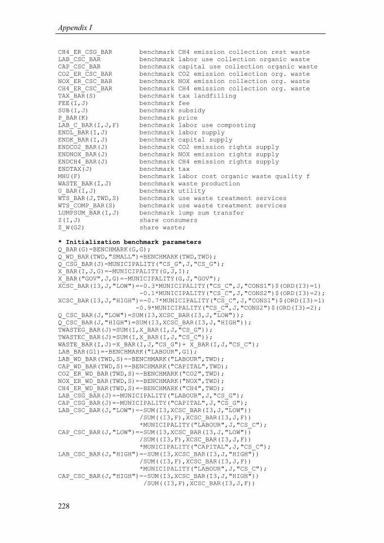
Appendix I
228
CH4_ER_CSG_BAR benchmark CH4 emission collection rest waste LAB_CSC_BAR benchmark labor use collection organic waste CAP_CSC_BAR benchmark capital use collection organic waste CO2_ER_CSC_BAR benchmark CO2 emission collection org. waste NOX_ER_CSC_BAR benchmark NOX emission collection org. waste CH4_ER_CSC_BAR benchmark CH4 emission collection org. waste TAX_BAR(S) benchmark tax landfilling FEE(I,J) benchmark fee SUB(I,J) benchmark subsidy P_BAR(K) benchmark price LAB_C_BAR(I,J,F) benchmark labor use composting ENDL_BAR(I,J) benchmark labor supply ENDK_BAR(I,J) benchmark capital supply ENDCO2_BAR(J) benchmark CO2 emission rights supply ENDNOX_BAR(J) benchmark NOX emission rights supply ENDCH4_BAR(J) benchmark CH4 emission rights supply ENDTAX(J) benchmark tax MHU(F) benchmark labor cost organic waste quality f WASTE_BAR(I,J) benchmark waste production U_BAR(I,J) benchmark utility WTS_BAR(J,TWD,S) benchmark use waste treatment services WTS_COMP_BAR(S) benchmark use waste treatment services LUMPSUM_BAR(I,J) benchmark lump sum transfer Z(I,J) share consumers Z_W(G2) share waste; * Initialization benchmark parameters
Q_BAR(G)=BENCHMARK(G,G); Q_WD_BAR(TWD,"SMALL")=BENCHMARK(TWD,TWD); Q_CSG_BAR(J)=MUNICIPALITY("CS_G",J,"CS_G"); X_BAR(I,J,G)=-MUNICIPALITY(G,J,I); X_BAR("GOV",J,G)=-MUNICIPALITY(G,J,"GOV"); XCSC_BAR(I3,J,"LOW")=-0.3*MUNICIPALITY("CS_C",J,"CONS1")$(ORD(I3)=1) -0.1*MUNICIPALITY("CS_C",J,"CONS2")$(ORD(I3)=2); XCSC_BAR(I3,J,"HIGH")=-0.7*MUNICIPALITY("CS_C",J,"CONS1")$(ORD(I3)=1) -0.9*MUNICIPALITY("CS_C",J,"CONS2")$(ORD(I3)=2); Q_CSC_BAR(J,"LOW")=SUM(I3,XCSC_BAR(I3,J,"LOW")); Q_CSC_BAR(J,"HIGH")=SUM(I3,XCSC_BAR(I3,J,"HIGH")); TWASTEG_BAR(J)=SUM(I,X_BAR(I,J,"CS_G")); TWASTEC_BAR(J)=SUM(I,X_BAR(I,J,"CS_C")); WASTE_BAR(I,J)=X_BAR(I,J,"CS_G")+ X_BAR(I,J,"CS_C"); LAB_BAR(G1)=-BENCHMARK("LABOUR",G1); LAB_WD_BAR(TWD,S)=-BENCHMARK("LABOUR",TWD); CAP_WD_BAR(TWD,S)=-BENCHMARK("CAPITAL",TWD); CO2_ER_WD_BAR(TWD,S)=-BENCHMARK("CO2",TWD); NOX_ER_WD_BAR(TWD,S)=-BENCHMARK("NOX",TWD); CH4_ER_WD_BAR(TWD,S)=-BENCHMARK("CH4",TWD); LAB_CSG_BAR(J)=-MUNICIPALITY("LABOUR",J,"CS_G"); CAP_CSG_BAR(J)=-MUNICIPALITY("CAPITAL",J,"CS_G"); LAB_CSC_BAR(J,"LOW")=-SUM(I3,XCSC_BAR(I3,J,"LOW")) /SUM((I3,F),XCSC_BAR(I3,J,F)) *MUNICIPALITY("LABOUR",J,"CS_C"); CAP_CSC_BAR(J,"LOW")=-SUM(I3,XCSC_BAR(I3,J,"LOW")) /SUM((I3,F),XCSC_BAR(I3,J,F)) *MUNICIPALITY("CAPITAL",J,"CS_C"); LAB_CSC_BAR(J,"HIGH")=-SUM(I3,XCSC_BAR(I3,J,"HIGH")) /SUM((I3,F),XCSC_BAR(I3,J,F)) *MUNICIPALITY("LABOUR",J,"CS_C"); CAP_CSC_BAR(J,"HIGH")=-SUM(I3,XCSC_BAR(I3,J,"HIGH")) /SUM((I3,F),XCSC_BAR(I3,J,F))

Specification of the model in GAMS
229
*MUNICIPALITY("CAPITAL",J,"CS_C"); CAP_BAR(G1)=-BENCHMARK("CAPITAL",G1); CO2_ER_BAR(G1)=-BENCHMARK("CO2",G1); NOX_ER_BAR(G1)=-BENCHMARK("NOX",G1); CH4_ER_BAR(G1)=-BENCHMARK("CH4",G1); TAX_BAR(S)=-BENCHMARK("TAX","CS_G"); FEE(I,J)=-MUNICIPALITY("FEE",J,I); SUB(I,J)=ABS(MUNICIPALITY("SUBSIDY",J,I)); P_BAR(K)=BENCHMARK(K,"PRICE"); MHU(F)=LABOUR_COMP("MHU",F); LAB_C_BAR(I3,J,F)=XCSC_BAR(I3,J,F)/MHU(F); ENDL_BAR(I4,J)=MUNICIPALITY("LABOUR",J,I4) +SUM(F,LAB_C_BAR("CONS1A",J,F))$(ORD(I4)=1) +SUM(F,LAB_C_BAR("CONS2A",J,F))$(ORD(I4)=2); ENDK_BAR(I,J)=MUNICIPALITY("CAPITAL",J,I); ENDCO2_BAR(J)=MUNICIPALITY("CO2",J,"GOV"); ENDNOX_BAR(J)=MUNICIPALITY("NOX",J,"GOV"); ENDCH4_BAR(J)=MUNICIPALITY("CH4",J,"GOV"); ENDTAX(J)=MUNICIPALITY("TAX",J,"GOV"); U_BAR(I3,J)=SUM(F,XCSC_BAR(I3,J,F)); WTS_BAR(J,TWD,"SMALL")=-MUNICIPALITY(TWD,J,"CS_G"); WTS_BAR(J,"COMP_L","SMALL")=-MUNICIPALITY("COMP_L",J,"CS_C"); WTS_BAR(J,"COMP_H","SMALL")=-MUNICIPALITY("COMP_H",J,"CS_C"); WTS_COMP_BAR(S)=-SUM(J,MUNICIPALITY("INCIN",J,"COMP_L")); *LUMPSUM_BAR(C,J)=CONSUMER("LUMPSUM",C,J); LUMPSUM_BAR(I,J)=ABS(MUNICIPALITY("LUMPSUM",J,I)); Z(I,J)=SHARE_CONSUMERS(J,I); Z_W(G2)=SHARE_WASTE("SHARE_W",G2); BETA(I4,J,G2)=Z_W(G2)*WASTE_BAR(I4,J)/SUM(G2A,X_BAR(I4,J,G2A)); * Definition parameters substitution elasticity
PARAMETERS RHO(G) subs. parameter labor versus capital and emission RHO2(G) subs. parameter capital versus emission RHO3 subs. parameter incineration versus landfilling RHO_C(I,J) subs. parameter rest waste versus organic waste RHO_F(I,J) subs. parameter low versus high quality org. waste RHO_U(I,J) subs. parameter consumption costs SIGMA_BAR(G) subs. elas. labor versus capital emission rights SIGMA2_BAR(G) subs. elas. capital versus emission rights SIGMA3_BAR subs. elas. incineration versus landfilling SIGMA_C_BAR(I,J) subs. elas. rest versus org. waste SIGMA_F_BAR(I,J) subs. elas. low versus high quality org. waste SIGMA_U_BAR(I,J) subs. elas. low versus high quality org. waste; * Initialization parameters substitution elasticity utility
SIGMA_BAR(G)=ELASTICITY_PROD("SIGMA_P",G); SIGMA2_BAR(G)=ELASTICITY_PROD("SIGMA_P2",G); SIGMA3_BAR=ELASTICITY_PROD("SIGMA_P3","CS_G"); SIGMA_C_BAR(I4,J)=ELASTICITY_CONS(I4,J,"SIGMA_C"); SIGMA_F_BAR(I3,J)=ELASTICITY_CONS("CONS1",J,"SIGMA_F")$(ORD(I3)=1) +ELASTICITY_CONS("CONS2",J,"SIGMA_F")$(ORD(I3)=2); SIGMA_U_BAR(I2,J)=ELASTICITY_CONS(I2,J,"SIGMA_U"); RHO(G)=(1-SIGMA_BAR(G))/SIGMA_BAR(G); RHO2(G1)=(1-SIGMA2_BAR(G1))/SIGMA2_BAR(G1); RHO2(TWD)=(1-SIGMA2_BAR(TWD))/SIGMA2_BAR(TWD); RHO3=(1-SIGMA3_BAR)/SIGMA3_BAR; RHO_C(I4,J)=(1-SIGMA_C_BAR(I4,J))/SIGMA_C_BAR(I4,J); RHO_F(I3,J)=(1-SIGMA_F_BAR(I3,J))/SIGMA_F_BAR(I3,J); RHO_F(I4,J)=RHO_F("CONS1A",J)$(ORD(I4)=1)+RHO_F("CONS2A",J)

Appendix I
230
$(ORD(I4)=2); RHO_U(I2,J)=(1-SIGMA_U_BAR(I2,J))/SIGMA_U_BAR(I2,J); U_BAR(I2,J)=SUM(G2,0.5*X_bar(I2,J,G2)**(-RHO_U(I2,J))) **(-1/RHO_U(I2,J)); * Definition parameters necessary for model
PARAMETERS THETA(*,K) value share of factor input THETA_U(I,J,G) value share consumption goods THETA_C(I,J,G) value share of waste THETA_F(I,J,F) value share quality organic waste THETA_CS(J,S) value share waste treatment options THETA_CSG(K,J) value share collection rest waste THETA_CSC(K,J,F) value share collection organic waste THETA_WD(*,TWD,S) value share waste treatment options MHU(F) labor cost quality organic waste Y(I,J) income Y_SUB(I,J) income Y0_SUB(I,J) benchmark income GAP(I,J) gap between income and expenditure TAU(G) tax rate XI(G,*) tax wedge rest waste XI_C(G,J,F) tax wedge organic waste NWT(I,J) Negishi weight NWTSUM sum Negishi weight NWTNORM normalization Negishi weight TRANS_CSG(J) transfer rest waste TRANS_CSC(J) transfer organic waste TRANS_WD transfer landfilling Y0(I,J) initial income RHOn parameter Negishi adjustment SMALL_P parameter iteration SCALE scaling parameter PT_CSG(J) price including subsidy rest waste PT_CSC(J,F) price including subsidy org. waste P(K) price P_CSG(J) price collection rest waste P_CSC(J,F) price collection organic waste P_WD(TWD,S) price waste disposal P_WD_BAR(TWD,S) benchmark price waste disposal P0(K) initial price TRANS_C(J) transfer SUMVAR parameter for iteration TAU(G) subsidy rate TRANS(I,J) transfers A(G) technology parameter A_WD(TWD,S) technology parameter waste disposal A_COMP(Tcomp) technology parameter composting A_CSC(J) technology parameter waste collection ITER iteration count SENSI sensitivity parameter SOLVES parameter needed for two scenarios PT price including subsidy; * Initialization technology parameter and prizes
A(G)=TECHNOLOGY("A",G); A_WD(TWD,S)=TECHNOLOGY_WD("A_WD",TWD,S); A_COMP("COMP_L")=0.8; A_COMP("COMP_H")=1.0; A_CSC(J)=1;
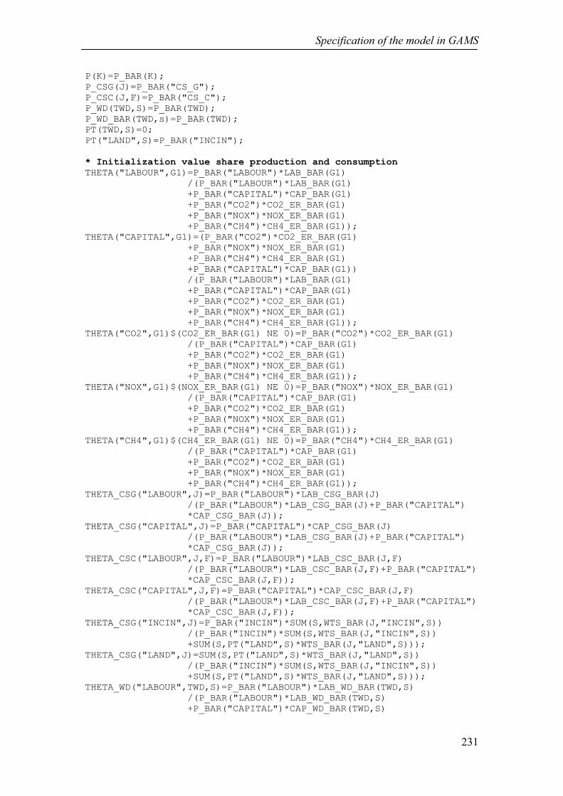
Specification of the model in GAMS
231
P(K)=P_BAR(K); P_CSG(J)=P_BAR("CS_G"); P_CSC(J,F)=P_BAR("CS_C"); P_WD(TWD,S)=P_BAR(TWD); P_WD_BAR(TWD,s)=P_BAR(TWD); PT(TWD,S)=0; PT("LAND",S)=P_BAR("INCIN"); * Initialization value share production and consumption
THETA("LABOUR",G1)=P_BAR("LABOUR")*LAB_BAR(G1) /(P_BAR("LABOUR")*LAB_BAR(G1) +P_BAR("CAPITAL")*CAP_BAR(G1) +P_BAR("CO2")*CO2_ER_BAR(G1) +P_BAR("NOX")*NOX_ER_BAR(G1) +P_BAR("CH4")*CH4_ER_BAR(G1)); THETA("CAPITAL",G1)=(P_BAR("CO2")*CO2_ER_BAR(G1) +P_BAR("NOX")*NOX_ER_BAR(G1) +P_BAR("CH4")*CH4_ER_BAR(G1) +P_BAR("CAPITAL")*CAP_BAR(G1)) /(P_BAR("LABOUR")*LAB_BAR(G1) +P_BAR("CAPITAL")*CAP_BAR(G1) +P_BAR("CO2")*CO2_ER_BAR(G1) +P_BAR("NOX")*NOX_ER_BAR(G1) +P_BAR("CH4")*CH4_ER_BAR(G1)); THETA("CO2",G1)$(CO2_ER_BAR(G1) NE 0)=P_BAR("CO2")*CO2_ER_BAR(G1) /(P_BAR("CAPITAL")*CAP_BAR(G1) +P_BAR("CO2")*CO2_ER_BAR(G1) +P_BAR("NOX")*NOX_ER_BAR(G1) +P_BAR("CH4")*CH4_ER_BAR(G1)); THETA("NOX",G1)$(NOX_ER_BAR(G1) NE 0)=P_BAR("NOX")*NOX_ER_BAR(G1) /(P_BAR("CAPITAL")*CAP_BAR(G1) +P_BAR("CO2")*CO2_ER_BAR(G1) +P_BAR("NOX")*NOX_ER_BAR(G1) +P_BAR("CH4")*CH4_ER_BAR(G1)); THETA("CH4",G1)$(CH4_ER_BAR(G1) NE 0)=P_BAR("CH4")*CH4_ER_BAR(G1) /(P_BAR("CAPITAL")*CAP_BAR(G1) +P_BAR("CO2")*CO2_ER_BAR(G1) +P_BAR("NOX")*NOX_ER_BAR(G1) +P_BAR("CH4")*CH4_ER_BAR(G1)); THETA_CSG("LABOUR",J)=P_BAR("LABOUR")*LAB_CSG_BAR(J) /(P_BAR("LABOUR")*LAB_CSG_BAR(J)+P_BAR("CAPITAL") *CAP_CSG_BAR(J)); THETA_CSG("CAPITAL",J)=P_BAR("CAPITAL")*CAP_CSG_BAR(J) /(P_BAR("LABOUR")*LAB_CSG_BAR(J)+P_BAR("CAPITAL") *CAP_CSG_BAR(J)); THETA_CSC("LABOUR",J,F)=P_BAR("LABOUR")*LAB_CSC_BAR(J,F) /(P_BAR("LABOUR")*LAB_CSC_BAR(J,F)+P_BAR("CAPITAL") *CAP_CSC_BAR(J,F)); THETA_CSC("CAPITAL",J,F)=P_BAR("CAPITAL")*CAP_CSC_BAR(J,F) /(P_BAR("LABOUR")*LAB_CSC_BAR(J,F)+P_BAR("CAPITAL") *CAP_CSC_BAR(J,F)); THETA_CSG("INCIN",J)=P_BAR("INCIN")*SUM(S,WTS_BAR(J,"INCIN",S)) /(P_BAR("INCIN")*SUM(S,WTS_BAR(J,"INCIN",S)) +SUM(S,PT("LAND",S)*WTS_BAR(J,"LAND",S))); THETA_CSG("LAND",J)=SUM(S,PT("LAND",S)*WTS_BAR(J,"LAND",S)) /(P_BAR("INCIN")*SUM(S,WTS_BAR(J,"INCIN",S)) +SUM(S,PT("LAND",S)*WTS_BAR(J,"LAND",S))); THETA_WD("LABOUR",TWD,S)=P_BAR("LABOUR")*LAB_WD_BAR(TWD,S) /(P_BAR("LABOUR")*LAB_WD_BAR(TWD,S) +P_BAR("CAPITAL")*CAP_WD_BAR(TWD,S)

Appendix I
232
+P_BAR("CO2")*CO2_ER_WD_BAR(TWD,S) +P_BAR("NOX")*NOX_ER_WD_BAR(TWD,S)+P_BAR("CH4") *CH4_ER_WD_BAR(TWD,S)); THETA_WD("ER_CAP",TWD,S)=(P_BAR("CAPITAL")*CAP_WD_BAR(TWD,S) +P_BAR("CO2")*CO2_ER_WD_BAR(TWD,S)+P_BAR("NOX") *NOX_ER_WD_BAR(TWD,S)+P_BAR("CH4") *CH4_ER_WD_BAR(TWD,S)) /(P_BAR("LABOUR")*LAB_WD_BAR(TWD,S) +P_BAR("CAPITAL")*CAP_WD_BAR(TWD,S) +P_BAR("CO2")*CO2_ER_WD_BAR(TWD,S) +P_BAR("NOX")*NOX_ER_WD_BAR(TWD,S)+P_BAR("CH4") *CH4_ER_WD_BAR(TWD,S)); THETA_WD("CAPITAL",TWD,S)=P_BAR("CAPITAL")*CAP_WD_BAR(TWD,S) /(P_BAR("CAPITAL")*CAP_WD_BAR(TWD,S) +P_BAR("CO2")*CO2_ER_WD_BAR(TWD,S) +P_BAR("NOX")*NOX_ER_WD_BAR(TWD,S)+P_BAR("CH4") *CH4_ER_WD_BAR(TWD,S)); THETA_WD("CO2",TWD,S)=P_BAR("CO2")*CO2_ER_WD_BAR(TWD,S) /(P_BAR("CAPITAL")*CAP_WD_BAR(TWD,S) +P_BAR("CO2")*CO2_ER_WD_BAR(TWD,S) +P_BAR("NOX")*NOX_ER_WD_BAR(TWD,S)+P_BAR("CH4") *CH4_ER_WD_BAR(TWD,S)); THETA_WD("NOX",TWD,S)=P_BAR("NOX")*NOX_ER_WD_BAR(TWD,S) /(P_BAR("CAPITAL")*CAP_WD_BAR(TWD,S) +P_BAR("CO2")*CO2_ER_WD_BAR(TWD,S) +P_BAR("NOX")*NOX_ER_WD_BAR(TWD,S)+P_BAR("CH4") *CH4_ER_WD_BAR(TWD,S)); THETA_WD("CH4",TWD,S)=P_BAR("CH4")*CH4_ER_WD_BAR(TWD,S) /(P_BAR("CAPITAL")*CAP_WD_BAR(TWD,S) +P_BAR("CO2")*CO2_ER_WD_BAR(TWD,S) +P_BAR("NOX")*NOX_ER_WD_BAR(TWD,S)+P_BAR("CH4") *CH4_ER_WD_BAR(TWD,S)); THETA_C(I4,J,"CS_G")=P_BAR("CS_G")*X_BAR(I4,J,"CS_G") /(P_BAR("CS_G")*X_BAR(I4,J,"CS_G")+P_BAR("CS_C") *X_BAR(I4,J,"CS_C")); THETA_C(I4,J,"CS_C")=P_BAR("CS_C")*X_BAR(I4,J,"CS_C") /(P_BAR("CS_G")*X_BAR(I4,J,"CS_G")+P_BAR("CS_C") *X_BAR(I4,J,"CS_C")); THETA_F(I3,J,F)=P_BAR("LABOUR")*LAB_C_BAR(I3,J,F)/(P_BAR("LABOUR") *SUM(F1,LAB_C_BAR(I3,J,F1))); THETA_F(I4,J,F)=(P_BAR("CS_C")*XCSC_BAR("CONS1A",J,F) /SUM(F1,P_BAR("CS_C")*XCSC_BAR("CONS1A",J,F1))) $(ORD(I4)=1) +(P_BAR("CS_C")*XCSC_BAR("CONS2A",J,F) /SUM(F1,P_BAR("CS_C")*XCSC_BAR("CONS2A",J,F1))) $(ORD(I4)=2); THETA_U(I2,J,"GOOD_WE")=P_BAR("GOOD_WE")*X_BAR(I2,J,"GOOD_WE") /(P_BAR("GOOD_WE")*X_BAR(I2,J,"GOOD_WE") +P_BAR("GOOD_WI")*X_BAR(I2,J,"GOOD_WI")); THETA_U(I2,J,"GOOD_WI")=P_BAR("GOOD_WI")*X_BAR(I2,J,"GOOD_WI") /(P_BAR("GOOD_WE")*X_BAR(I2,J,"GOOD_WE") +P_BAR("GOOD_WI")*X_BAR(I2,J,"GOOD_WI"));
* Definition parameters transport costs
PARAMETERS transport T(J,TWD,S) transport matrix TC transport costs TS_BAR(J,TWD,S) benchmark demand transport services;

Specification of the model in GAMS
233
* Initialization parameters transport costs
T(J,TWD,S)=TRANSPORT(TWD,S,J); TC=P("TRANS"); TS_BAR(J,TWD,S)=T(J,TWD,S)*WTS_BAR(J,TWD,S)/1000; * Initialization income and Negishi weights
Y(C,J)=P_BAR("CAPITAL")*ENDK_BAR(C,J)+P_BAR("LABOUR")*(ENDL_BAR(C,J)) -FEE(C,J)-LUMPSUM_BAR(C,J) -(P_BAR("LABOUR")*SUM(F,LAB_C_BAR("CONS1A",J,F))) $(ORD(C)=1) -(P_BAR("LABOUR")*SUM(F,LAB_C_BAR("CONS2A",J,F))) $(ORD(C)=2); Y("GOV",J)=P("TAX")*ENDTAX(J)+P_BAR("CO2")*ENDCO2_BAR(J) +P_BAR("NOX")*ENDNOX_BAR(J) +P_BAR("CH4")*ENDCH4_BAR(J)+SUM((C),FEE(C,J)) -SUB("GOV",J)+SUM((C),LUMPSUM_BAR(C,J)); Y("CONS1A",J)=P_BAR("LABOUR")*SUM(F,LAB_C_BAR("CONS1A",J,F)); Y("CONS2A",J)=P_BAR("LABOUR")*SUM(F,LAB_C_BAR("CONS2A",J,F)); FEE("GOV",J)=0; NWT(I,J)=Y(I,J)/SUM((I1,J1),Y(I1,J1)); XI("CS_G","M1")=-((P_BAR("CS_G")/P_BAR("GOOD_WE")) *NWT("GOV","m1")*100) /(X_BAR("GOV","m1","GOOD_WE") -(3*P_BAR("LAND")/P_BAR("CS_G") *3-16*P_BAR("CS_C")/P_BAR("CS_G")-4)*(P_BAR("CS_G") /P_BAR("GOOD_WE"))*NWT("GOV","m1")); XI("CS_G",J)=XI("CS_G","M1"); XI_C("CS_C",J,F)=P_BAR("CS_C")/P_BAR("CS_G")*XI("CS_G","M1"); XI("LAND",S)=-3*P_BAR("LAND")/P_BAR("CS_G")*XI("CS_G","M1"); TRANS_CSG(J)=XI("CS_G",J)*SUM(I,X_BAR(I,J,"CS_G")); TRANS_CSC(J)=XI("CS_C",J)*SUM(I,X_BAR(I,J,"CS_C")); TRANS_WD("LAND",J)=-MUNICIPALITY("TAX",J,"CS_G"); NWTNORM=100+SUM(J,XI("CS_G",J))+SUM(S,XI("LAND",S)) +SUM((J,F),XI_C("CS_C",J,F)); NWTSUM=SUM((I,J),NWT(I,J)); NWT(I,J)=NWT(I,J)*NWTNORM/NWTSUM; TAU("CS_C")=-1; TAU("CS_G")=-1; TAU("LAND")=3; ITER=0; * Definition of dummy parameter to ensure that inaction of waste
* treatment unit is possible
PARAMETER M(K,TWD,S) dummy
* Initialization of dummy parameter
M("CAPITAL",TWD,S)=0.0001*CAP_WD_BAR(TWD,S) /(CAP_WD_BAR(TWD,S)+LAB_WD_BAR(TWD,S)); M("LABOUR",TWD,S)=0.0001*LAB_WD_BAR(TWD,S) /(CAP_WD_BAR(TWD,S)+LAB_WD_BAR(TWD,S)); * Initialization of benchmark waste treatment middle and large units
CAP_WD_BAR(TWD,"MIDDLE")=0; LAB_WD_BAR(TWD,"MIDDLE")=0; WTS_COMP_BAR("MIDDLE")=0; TAX_BAR("MIDDLE")=0; CAP_WD_BAR(TWD,"B")=0; LAB_WD_BAR(TWD,"B")=0; WTS_COMP_BAR("B")=0;

Appendix I
234
TAX_BAR("B")=0; * Definition variables
POSITIVE VARIABLES Q(G) production Q_CSG production collection services rest waste Q_CSC(J,F) production collection services organic waste Q_WD(TWD,S) production waste disposal services X(I2,J,G) consumption CAP(G) capital use CAP_CSG capital use collection rest waste CAP_CSC capital use collection organic waste CAP_WD(TWD,S) capital use waste treatment LAB(G) labor use LAB_CSG labor use collection rest waste LAB_CSC labor use collection organic waste LAB_WD(TWD,S) labor use waste treatment TAX(S) tax landfilling U(I,J) utility TWG total supply rest waste TWC total supply organic waste ENDOWL(I4,J) labor supply WASTE(I,J) generation waste XCSC(I,J,F) quality organic waste LAB_C(I,J,F) labor use composting WTS(J,TWD,S) use waste treatment services WTS_COMP(S) use waste treatment services TS(J,TWD,S) transport services X_R_WASTE(I,J) rest waste X_O_WASTE(I,J,F) organic waste O_WASTE total organic waste Tland total demand landfilling services; VARIABLES WELFARE total welfare; * Definition equations
EQUATIONS QWELFARE equation total welfare QUTIL(I,J) utility function QUTIL2(I,J) utility function QPROD(G) production function goods QPRODWD(TWD,S) production function waste disposal services QPRODWD2(S) production function waste disposal services QPRODCSG_1 production function collection rest waste QPRODCSG_2 production function collection rest waste QPRODCSG_2B production function collection rest waste QPRODCSG_3 production function collection rest waste QPRODCSC_1 production function collection organic waste QPRODCSC_2 production function collection organic waste QPRODCSC_2B production function collection organic waste QPRODCSC_3 production function collection organic waste QPRODCSC_3B production function collection organic waste QPRODCSC_3C(J,S) production function collection organic waste QBALFACL balance equation labor QBALFACK balance equation capital QBALFACCO2 balance equation CO2 QBALFACNOX balance equation NOX QBALFACCH4 balance equation CH4 QBALWTS_INCIN balance equation incineration

Specification of the model in GAMS
235
QBALWTS_INCIN2 balance equation incineration QBALWTS2 balance equation composting services QBALLAND1 balance equation landfilling QBALLAND2 balance equation landfilling QBALTRANS balance function transportation services QBALGOOD balance equation demand good QPRODW1 production function waste QPRODW2 production function waste QBALCSG1 balance equation collection rest waste flat fee QBALCSG2 balance equation collection rest waste flat fee QBALCSG3 balance equation collection rest waste unit price QBALCSC1 balance equation collection compost flat fee QBALCSC2 balance equation collection compost flat fee QPRODENDL calculation labor availability QPRODXCSC production organic waste QBALCOMPOST balance compost virtual consumer QBALTS_1(J,TWD,S) balance equation demand transport services QPRODWASTE1 equation calculating rest waste in tons QPRODWASTE2 equation calculating organic waste in tonnes QPRODWASTE2A(I3,J,F) equation calculating organic waste in tonnes QPRODWASTE3 equation calculating organic waste in tonnes; * Total welfare function
QWELFARE.. WELFARE=E=SUM(J,NWT("GOV",J)*LOG(U("GOV",J))) +SUM((C,J),NWT(C,J)*LOG(U(C,J))) -SUM(J,XI("CS_G",J)*TWG(J)) -SUM((J,F),XI_C("CS_C",J,F)*TWC(J,F)) -SUM(S,XI("LAND",S)*TLAND(S)); * Calculation utility consumer
QUTIL(I2,J).. U(I2,J)=L=U_BAR(I2,J)*(THETA_U(I2,J,"GOOD_WE") *(X(I2,J,"GOOD_WE")/X_BAR(I2,J,"GOOD_WE")) **(-RHO_U(I2,J)) +(THETA_U(I2,J,"GOOD_WI") *(X(I2,J,"GOOD_WI")/X_BAR(I2,J,"GOOD_WI")) **(-RHO_U(I2,J))) $(THETA_U(I2,J,"GOOD_WI") NE 0)) **(-1/RHO_U(I2,J)); QUTIL2(I3,J).. U(I3,J)=L=U_BAR(I3,J)*(THETA_F(I3,J,"LOW") *(LAB_C(I3,J,"LOW")/LAB_C_BAR(I3,J,"LOW")) **(-RHO_F(I3,J)) + THETA_F(I3,J,"HIGH") *(LAB_C(I3,J,"HIGH") /LAB_C_BAR(I3,J,"HIGH")) **(-RHO_F(I3,J)))**(-1/RHO_F(I3,J)); * Production function consumption good and transport services
QPROD(G1).. Q(G1)=L=A(G1)*Q_BAR(G1)* (THETA("LABOUR",G1)*(LAB(G1)/LAB_BAR(G1)) **(-RHO(G1)) +THETA("CAPITAL",G1)*(CAP(G1)/CAP_BAR(G1)) **(-RHO(G1)))**(-1/RHO(G1)); * Nested CES Leontief production function collection rest waste
QPRODCSG_1(J).. Q_CSG(J)=L=A("CS_G")*Q_CSG_BAR(J) *(THETA_CSG("CAPITAL",J) *(CAP_CSG(J)/CAP_CSG_BAR(J)) **(-RHO("CS_G")) +THETA_CSG("LABOUR",J) *(LAB_CSG(J)/LAB_CSG_BAR(J)) **(-RHO("CS_G"))) **(-1/RHO("CS_G")); QPRODCSG_2(J).. Q_CSG(J)=L=Q_CSG_BAR(J)
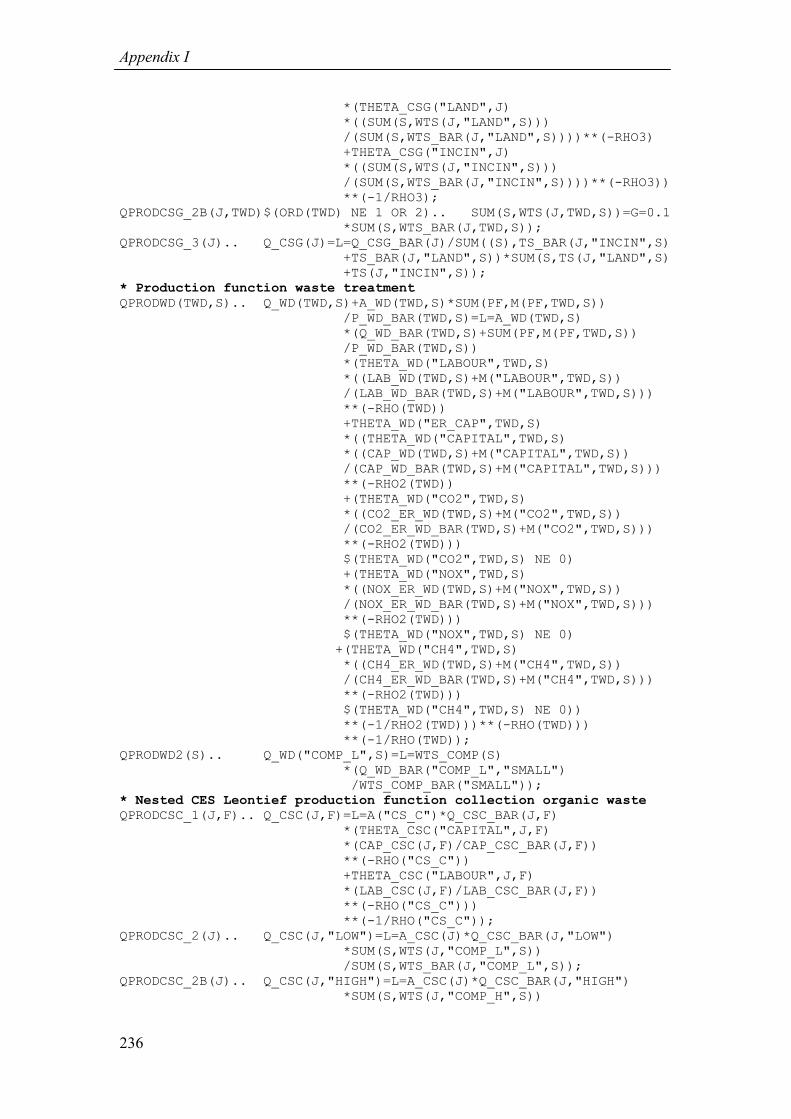
Appendix I
236
*(THETA_CSG("LAND",J) *((SUM(S,WTS(J,"LAND",S))) /(SUM(S,WTS_BAR(J,"LAND",S))))**(-RHO3) +THETA_CSG("INCIN",J) *((SUM(S,WTS(J,"INCIN",S))) /(SUM(S,WTS_BAR(J,"INCIN",S))))**(-RHO3)) **(-1/RHO3); QPRODCSG_2B(J,TWD)$(ORD(TWD) NE 1 OR 2).. SUM(S,WTS(J,TWD,S))=G=0.1 *SUM(S,WTS_BAR(J,TWD,S)); QPRODCSG_3(J).. Q_CSG(J)=L=Q_CSG_BAR(J)/SUM((S),TS_BAR(J,"INCIN",S) +TS_BAR(J,"LAND",S))*SUM(S,TS(J,"LAND",S) +TS(J,"INCIN",S)); * Production function waste treatment
QPRODWD(TWD,S).. Q_WD(TWD,S)+A_WD(TWD,S)*SUM(PF,M(PF,TWD,S)) /P_WD_BAR(TWD,S)=L=A_WD(TWD,S) *(Q_WD_BAR(TWD,S)+SUM(PF,M(PF,TWD,S)) /P_WD_BAR(TWD,S)) *(THETA_WD("LABOUR",TWD,S) *((LAB_WD(TWD,S)+M("LABOUR",TWD,S)) /(LAB_WD_BAR(TWD,S)+M("LABOUR",TWD,S))) **(-RHO(TWD)) +THETA_WD("ER_CAP",TWD,S) *((THETA_WD("CAPITAL",TWD,S) *((CAP_WD(TWD,S)+M("CAPITAL",TWD,S)) /(CAP_WD_BAR(TWD,S)+M("CAPITAL",TWD,S))) **(-RHO2(TWD)) +(THETA_WD("CO2",TWD,S) *((CO2_ER_WD(TWD,S)+M("CO2",TWD,S)) /(CO2_ER_WD_BAR(TWD,S)+M("CO2",TWD,S))) **(-RHO2(TWD))) $(THETA_WD("CO2",TWD,S) NE 0) +(THETA_WD("NOX",TWD,S) *((NOX_ER_WD(TWD,S)+M("NOX",TWD,S)) /(NOX_ER_WD_BAR(TWD,S)+M("NOX",TWD,S))) **(-RHO2(TWD))) $(THETA_WD("NOX",TWD,S) NE 0) +(THETA_WD("CH4",TWD,S) *((CH4_ER_WD(TWD,S)+M("CH4",TWD,S)) /(CH4_ER_WD_BAR(TWD,S)+M("CH4",TWD,S))) **(-RHO2(TWD))) $(THETA_WD("CH4",TWD,S) NE 0)) **(-1/RHO2(TWD)))**(-RHO(TWD))) **(-1/RHO(TWD)); QPRODWD2(S).. Q_WD("COMP_L",S)=L=WTS_COMP(S) *(Q_WD_BAR("COMP_L","SMALL") /WTS_COMP_BAR("SMALL")); * Nested CES Leontief production function collection organic waste
QPRODCSC_1(J,F).. Q_CSC(J,F)=L=A("CS_C")*Q_CSC_BAR(J,F) *(THETA_CSC("CAPITAL",J,F) *(CAP_CSC(J,F)/CAP_CSC_BAR(J,F)) **(-RHO("CS_C")) +THETA_CSC("LABOUR",J,F) *(LAB_CSC(J,F)/LAB_CSC_BAR(J,F)) **(-RHO("CS_C"))) **(-1/RHO("CS_C")); QPRODCSC_2(J).. Q_CSC(J,"LOW")=L=A_CSC(J)*Q_CSC_BAR(J,"LOW") *SUM(S,WTS(J,"COMP_L",S)) /SUM(S,WTS_BAR(J,"COMP_L",S)); QPRODCSC_2B(J).. Q_CSC(J,"HIGH")=L=A_CSC(J)*Q_CSC_BAR(J,"HIGH") *SUM(S,WTS(J,"COMP_H",S))

Specification of the model in GAMS
237
/SUM(S,WTS_BAR(J,"COMP_H",S)); QPRODCSC_3(J).. Q_CSC(J,"LOW")=L=A_CSC(J)*Q_CSC_BAR(J,"LOW") /SUM((S),TS_BAR(J,"COMP_L",S)) *SUM((S),TS(J,"COMP_L",S)); QPRODCSC_3B(J).. Q_CSC(J,"HIGH")=L=A_CSC(J)*Q_CSC_BAR(J,"HIGH") /SUM((S),TS_BAR(J,"COMP_H",S)) *SUM((S),TS(J,"COMP_H",S)); QPRODCSC_3C(J,S).. WTS(J,"COMP_L",S)/Q_CSC(J,"LOW")=E= WTS(J,"COMP_H",S)/Q_CSC(J,"HIGH"); * Balance equation labor, capital, and emission rights
QBALFACL.. SUM(G1,LAB(G1))+SUM(J,LAB_CSG(J)) +SUM((J,F),LAB_CSC(J,F)) +SUM((TWD,S),LAB_WD(TWD,S))=L= SUM((I4,J),ENDOWL(I4,J)); QBALFACK.. SUM(G1,CAP(G1))+SUM(J,CAP_CSG(J)) +SUM((J,F),CAP_CSC(J,F)) +SUM((TWD,S),CAP_WD(TWD,S))=L= SUM((I,J),ENDK_BAR(I,J)); * Balance equation demand incineration services
QBALWTS_INCIN.. SUM((J),WTS(J,"INCIN","SMALL")) +SUM((S),WTS_COMP(S))=L=Q_WD("INCIN","SMALL"); QBALWTS_INCIN2(S)$(ORD(S) NE 1).. SUM((J),WTS(J,"INCIN",S)) =L=Q_WD("INCIN",S); * Balance equation demand composting services
QBALWTS2(TCOMP,S).. SUM((J),WTS(J,TCOMP,S))=L=Q_WD(TCOMP,S); * Balance equation demand waste treatment
QBALLAND1(S).. SUM(J,WTS(J,"LAND",S))=E=TLAND(S); QBALLAND2(S).. TLAND(S)=E=Q_WD("LAND",S); * Demand transport services
QBALTS_1(J,TWD,S).. TS(J,TWD,S)=E=T(J,TWD,S)*WTS(J,TWD,S)/1000; * Balance equation demand transport services
QBALTRANS.. SUM((J,TWD,S),TS(J,TWD,S))=L=Q("TRANS"); * Balance equation demand consumption good
QBALGOOD(G2).. SUM((I2,J),X(I2,J,G2))=L=Q(G2); * Generation waste as function consumption
QPRODW1(I4,J).. WASTE(I4,J)=E=SUM(G2,BETA(I4,J,G2)*X(I4,J,G2)); * Demand collection services
QPRODW2(I4,J).. WASTE(I4,J)=E=WASTE_BAR(I4,J) *(THETA_C(I4,J,"CS_G") *(X(I4,J,"CS_G")/X_BAR(I4,J,"CS_G")) **(-RHO_C(I4,J)) +THETA_C(I4,J,"CS_C")* ((THETA_F(I4,J,"LOW") *(((XCSC(I4,J,"LOW") +XCSC("CONS1A",J,"LOW")) /XCSC_BAR("CONS1A",J,"LOW"))$(ORD(I4)=1) + (((XCSC(I4,J,"LOW") +XCSC("CONS2A",J,"LOW")) /XCSC_BAR("CONS2A",J,"LOW"))) $(ORD(I4)=2))**(-RHO_F(I4,J)) +THETA_F(I4,J,"HIGH") *((((XCSC(I4,J,"HIGH") +XCSC("CONS1A",J,"HIGH")) /XCSC_BAR("CONS1A",J,"HIGH"))) $(ORD(I4)=1) + (((XCSC(I4,J,"HIGH") +XCSC("CONS2A",J,"HIGH")) /XCSC_BAR("CONS2A",J,"HIGH"))) $(ORD(I4)=2)) **(-RHO_F(I4,J)))**(-1/RHO_F(I4,J)))

Appendix I
238
**(-RHO_C(I4,J)))**(-1/RHO_C(I4,J)); * Calculation demand collection services in tonnes
QPRODWASTE1(I4,J).. X_R_WASTE(I4,J)=E=X(I4,J,"CS_G"); QPRODWASTE2(I4,J,F).. X_O_WASTE(I4,J,F)=E=(XCSC(I4,J,F) +XCSC("CONS1A",J,F)$(ORD(I4)=1) +XCSC("CONS2A",J,F)$(ORD(I4)=2)) /SUM(F1,XCSC(I4,J,f1) +XCSC("CONS1A",J,F1)$(ORD(I4)=1) +XCSC("CONS2A",J,F1)$(ORD(I4)=2)) *(WASTE(I4,J)-X(I4,J,"CS_G")); QPRODWASTE2A(I3,J,F).. X_O_WASTE(I3,J,F)=E=XCSC(I3,J,F) /(SUM(F1,XCSC(I3,J,F1) +XCSC("CONS1",J,F1)$(ORD(I3)=1) +XCSC("CONS2",J,F1)$(ORD(I3)=2))) *((WASTE("CONS1",J) -X("CONS1",J,"CS_G"))$(ORD(I3)=1) +(WASTE("CONS2",J) -X("CONS2",J,"CS_G"))$(ORD(I3)=2)); QPRODWASTE3(I4,J).. X_R_WASTE(I4,J)+SUM(F,X_O_WASTE(I4,J,F)) =E=WASTE(I4,J); * Balance equation demand collection rest waste
QBALCSG1(J)$(SOLVES=0).. SUM(I4,X_R_WASTE(I4,J))=E=TWG(J); QBALCSG2(J)$(SOLVES=0).. TWG(J)=E=Q_CSG(J); QBALCSG3(J)$(SOLVES=1).. SUM(I4,X_R_WASTE(I4,J))=L=Q_CSG(J); * Balance equation demand collection organic waste
QBALCSC1(J,F).. SUM((I4),X_O_WASTE(I4,J,F))=E=TWC(J,F); QBALCSC2(J,F).. TWC(J,F)=E=Q_CSC(J,F); *QBALCSC3$(SOLVES=1).. SUM((C,F),XCSC(I,J,F))=L=Q("CS_C"); * Calculation labor supply endogenously determined in model
QPRODENDL(I4,J).. ENDOWL(I4,J)=L=ENDL_BAR(I4,J) -SUM(F,LAB_C(I4,J,F)) -(SUM(F,LAB_C("CONS1A",J,F)))$(ORD(I4)=1) -(SUM(F,LAB_C("CONS2A",J,F))) $(ORD(I4)=2); * Labor input generation organic waste
QPRODXCSC(C,J,F).. XCSC(C,J,F)=E=MHU(F)*LAB_C(C,J,F); * Equation ensuring that organic waste is generated in benchmark
QBALCOMPOST(I3,J).. SUM(F,LAB_C(I3,J,F))=L= SUM(F,Lab_C_BAR(I3,J,F)); * Definition of model
MODEL QUALITY /ALL/; QUALITY.SCALEOPT=1; * Defining lower and upper bounds variables
Q.LO(G1)=0.1*Q_BAR(G1); Q.UP(G1)=10*Q_BAR(G1); Q_CSC.LO(J,F)=0.1*Q_CSC_BAR(J,F); Q_CSC.UP(J,F)=10*Q_CSC_BAR(J,F); Q_CSG.LO(J)=0.1*Q_CSG_BAR(J); Q_CSG.UP(J)=10*Q_CSG_BAR(J); Q_WD.UP(TWD,S)=10*Q_WD_BAR(TWD,"SMALL"); X.LO(I4,J,"GOOD_WE")=0.1*X_BAR(I4,J,"GOOD_WE"); X.LO(I4,J,"GOOD_WI")=0.1*X_BAR(I4,J,"GOOD_WI"); X.LO(I4,J,"CS_G")=0.1*X_BAR(I4,J,"CS_G"); X.LO("GOV",J,"GOOD_WE")=0.1*X_BAR("GOV",J,"GOOD_WE"); X.FX("GOV",J,"GOOD_WI")=0; X.UP(I2,J,G)=10*X_BAR(I2,J,G); CAP.LO(G1)=0.1*CAP_BAR(G1);

Specification of the model in GAMS
239
LAB.LO(G1)=0.1*LAB_BAR(G1); CAP.UP(G1)=10*CAP_BAR(G1); LAB.UP(G1)=10*LAB_BAR(G1); CAP_WD.UP(TWD,S)=10*CAP_WD_BAR(TWD,"SMALL"); LAB_WD.UP(TWD,S)=10*LAB_WD_BAR(TWD,"SMALL"); WTS_COMP.UP(S)=10*WTS_COMP_BAR("SMALL"); CAP_CSG.LO(J)=0.1*CAP_CSG_BAR(J); LAB_CSG.LO(J)=0.1*LAB_CSG_BAR(J); CAP_CSG.UP(J)=10*CAP_CSG_BAR(J); LAB_CSG.UP(J)=10*LAB_CSG_BAR(J); CAP_CSC.LO(J,F)=0.1*CAP_CSC_BAR(J,F); LAB_CSC.LO(J,F)=0.1*LAB_CSC_BAR(J,F); CAP_CSC.UP(J,F)=10*CAP_CSC_BAR(J,F); LAB_CSC.UP(J,F)=10*LAB_CSC_BAR(J,F); U.LO(I,J)=0.1*U_BAR(I,J); TWG.LO(J)=0.1*TWASTEG_BAR(J); TWC.LO(J,F)=0.1*TWASTEC_BAR(J); TWG.UP(J)=10*TWASTEG_BAR(J); TWC.UP(J,F)=10*TWASTEC_BAR(J); ENDOWL.LO(I4,J)=0.9*ENDL_BAR(I4,J); ENDOWL.UP(I4,J)=ENDL_BAR(I4,J); WASTE.LO(I4,J)=0.1*WASTE_BAR(I4,J); WASTE.UP(I4,J)=10*WASTE_BAR(I4,J); XCSC.LO(I3,J,F)=0.9*XCSC_BAR(I3,J,F); XCSC.UP(I3,J,F)=1.5*XCSC_BAR(I3,J,F); XCSC.UP(I4,J,F)=10*XCSC_BAR("CONS1A",J,F)$(ORD(I4)=1) +10*XCSC_BAR("CONS2A",J,F)$(ORD(I4)=2); X.LO(I4,J,"CS_G")=0.1*X_BAR(I4,J,"CS_G"); X.UP(I4,J,"CS_G")=10*X_BAR(I4,J,"CS_G"); X_O_WASTE.LO(C,J,F)=0.1*XCSC_BAR(C,J,F); X_O_WASTE.UP(I3,J,F)=10*XCSC_BAR(I3,J,F); X_O_WASTE.UP(I4,J,F)=10*XCSC_BAR("CONS1A",J,F)$(ORD(I4)=1) +10*XCSC_BAR("CONS2A",J,F)$(ORD(I4)=2); XCSC.FX("GOV",J,F)=0; LAB_C.UP(I4,J,F)=0.02*ENDL_BAR(I4,J); LAB_C.LO(I3,J,F)=0.5*LAB_C_BAR(I3,J,F); LAB_C.UP(I3,J,F)=1.5*LAB_C_BAR(I3,J,F); WTS.UP(J,TWD,S)=10*WTS_BAR(J,TWD,"SMALL"); TS.UP(J,TWD,S)=10*TS_BAR(J,TWD,"SMALL"); U.UP(I,J)=10*U_BAR(I,J); TLAND.UP(S)=10*Q_WD_BAR("LAND","SMALL"); * Defining initial levels of variables Q.L(G)=Q_BAR(G); Q.L("TRANS")=Q_BAR("TRANS"); Q_WD.L(TWD,S)=Q_WD_BAR(TWD,S); Q_WD.L(TWD,"MIDDLE")=0; Q_WD.L(TWD,"B")=0; Q_CSG.L(J)=Q_CSG_BAR(J); Q_CSC.L(J,F)=Q_CSC_BAR(J,F); X.L(I2,J,G)=X_BAR(I2,J,G); X.L("GOV",J,G)=X_BAR("GOV",J,G); CAP.L(G1)=CAP_BAR(G1); LAB.L(G1)=LAB_BAR(G1); CO2_ER.L(G1)=CO2_ER_BAR(G1); NOX_ER.L(G1)=NOX_ER_BAR(G1); CH4_ER.L(G1)=CH4_ER_BAR(G1); CAP_WD.L(TWD,"SMALL")=CAP_WD_BAR(TWD,"SMALL"); LAB_WD.L(TWD,"SMALL")=LAB_WD_BAR(TWD,"SMALL"); WTS_COMP.L("SMALL")=WTS_COMP_BAR("SMALL");
Appendix I
240
CO2_ER_WD.L(TWD,"SMALL")=CO2_ER_WD_BAR(TWD,"SMALL"); NOX_ER_WD.L(TWD,"SMALL")=NOX_ER_WD_BAR(TWD,"SMALL"); CH4_ER_WD.L(TWD,"SMALL")=CH4_ER_WD_BAR(TWD,"SMALL"); WTS.L(J,"LAND",S)=WTS_BAR(J,"LAND",S); WTS.L(J,"INCIN",S)=WTS_BAR(J,"INCIN",S); WTS.L(J,TCOMP,S)=WTS_BAR(J,TCOMP,S); TS.L(J,TWD,S)=TS_BAR(J,TWD,S); CAP_CSG.L(J)=CAP_CSG_BAR(J); LAB_CSG.L(J)=LAB_CSG_BAR(J); CAP_CSC.L(J,F)=CAP_CSC_BAR(J,F); LAB_CSC.L(J,F)=LAB_CSC_BAR(J,F); U.L(I2,J)=U_BAR(I2,J); U.L("GOV",J)=U_BAR("GOV",J); U.L(I3,J)=U_BAR(I3,J); TWG.L(J)=TWASTEG_BAR(J); TWC.L(J,"LOW")=SUM(I3,XCSC_BAR(I3,J,"LOW")) /SUM((I3,F),XCSC_BAR(I3,J,F))*TWASTEC_BAR(J); TWC.L(J,"HIGH")=SUM(I3,XCSC_BAR(I3,J,"HIGH")) /SUM((I3,F),XCSC_BAR(I3,J,F))*TWASTEC_BAR(J); ENDOWL.L("CONS1",J)=ENDL_BAR("CONS1",J) -SUM(F,LAB_C_BAR("CONS1A",J,F)); ENDOWL.L("CONS2",J)=ENDL_BAR("CONS2",J) -SUM(F,LAB_C_BAR("CONS2A",J,F)); WASTE.L(I,J)=X_BAR(I,J,"CS_G")+X_BAR(I,J,"CS_C"); XCSC.L(I,J,F)=XCSC_BAR(I,J,F); X_R_WASTE.L(I4,J)=X_BAR(I4,J,"CS_G"); X_O_WASTE.L(I4,J,F)=XCSC_BAR("CONS1A",J,F)$(ORD(I4)=1) +XCSC_BAR("CONS2A",J,F)$(ORD(I4)=2); X_O_WASTE.L(I3,J,F)=XCSC_BAR(I3,J,F); LAB_C.L(I,J,F)=LAB_C_BAR(I,J,F); TLAND.L(S)=Q_WD_BAR("LAND",S); * Defining parameters for iteration
RHOn = 0.030; SMALL_P = 0.000018; SUMVAR=1000; GAP(I,J)=0; * Include files for report writing
$INCLUDE "PARAMETER_IO_TABLE_S10.GMS"; $INCLUDE "BENCHMARK_IO_TABLE_S10.GMS"; $INCLUDE "EMISSION_TABLE_S10.GMS"; * Start loop for finding equilibrium solution for flat fee and unit-
based price
LOOP(SCEN, * Parameter value in flat fee scenario
IF(FLAT(scen), solves = 0; * Change values parameters in unit-based price scenario
ELSE solves = 1; TWG.FX(J)=0; TWC.L(J,F)=TWASTEC_BAR(J); FEE("CONS1",J)=-MUNICIPALITY("CS_C",J,"CONS1") *P_BAR("CS_C")/1.06; FEE("CONS2",J)=-MUNICIPALITY("CS_C",J,"CONS2") *P_BAR("CS_C")/1.06;

Specification of the model in GAMS
241
SUB("GOV",J)=1.06*SUM(I4,FEE(I4,J)); XI("CS_G",J)=0; TAU("CS_G")=0; SUMVAR=1000; ITER=0; TRANS(I,J)=0; TRANS_CSG(J)=0; ); * Start loop for determining optimal Negishi weights
LOOP (ITWEL $(SUMVAR GT SMALL_P), ITER = ITER+1; * Solve model
SOLVE QUALITY USING DNLP MAXIMIZING WELFARE; * Calculate prices, income and budget constraint
P0(K)=P(K); P("CAPITAL")=ABS(QBALFACK.M); P("LABOUR")=ABS(QBALFACL.M); P(G2)=ABS(QBALGOOD.M(G2)); PT_CSG(J)=ABS(QBALCSG1.M(J))$(SOLVES=0)+0$(SOLVES=1); P_CSG(J)=ABS(QBALCSG2.M(J))$(SOLVES=0) +ABS(QBALCSG3.M(J))$(SOLVES=1); PT_CSC(J,F)=ABS(QBALCSC1.M(J,F)); P_CSC(J,F)=ABS(QBALCSC2.M(J,F)); P("TRANS")=ABS(QBALTRANS.M); P_WD("INCIN",S)$(ORD(S)=1)=ABS(QBALWTS_INCIN.M); P_WD("INCIN",S)$(ORD(S) NE 1)=ABS(QBALWTS_INCIN2.M(S)); P_WD(TCOMP,S)=ABS(QBALWTS2.M(TCOMP,S)); P("CO2")=ABS(QBALFACCO2.M); P("NOX")=ABS(QBALFACNOX.M); P("CH4")=ABS(QBALFACCH4.M); PT("LAND",S)=ABS(QBALLAND1.M(S)); P_WD("LAND",S)=ABS(QBALLAND2.M(S)); SCALE=P("CAPITAL"); XI("CS_G",J)=TAU("CS_G")*P_CSG(J); XI_C("CS_C",J,F)=TAU("CS_C")*P_CSC(J,F); XI("LAND",S)=TAU("LAND")*P_WD("LAND",S); P(K)=P(K)/SCALE; P("CS_G")=0; P("CS_C")=0; P_CSC(J,F)=P_CSC(J,F)/SCALE; P_CSG(J)=P_CSG(J)/SCALE; P_WD(TWD,S)=P_WD(TWD,S)/SCALE; P(TWD)=P_WD(TWD,"SMALL"); TRANS_CSG(J)=SUM((I4),XI("CS_G",J)/SCALE*X_R_WASTE.L(I4,J)); TRANS_CSC(J)=SUM((I4,F),XI_C("CS_C",J,F)/SCALE *X_O_WASTE.L(I4,J,F)); TRANS_WD("LAND",J)=SUM((S),XI("LAND",S)/SCALE*WTS.L(J,"LAND",S)); PT_CSG(J)=PT_CSG(J)/SCALE; PT_CSC(J,F)=PT_CSC(J,F)/SCALE; PT("LAND",S)=PT("LAND",S)/SCALE; p("tax")=p0("tax"); TRANS("GOV",J)=TRANS_CSG(J)+TRANS_CSC(J)+TRANS_WD("LAND",J); Y0(I,J)=Y(I,J); Y("GOV",J)=P("CO2")*ENDCO2_BAR(J)+P("NOX")*ENDNOX_BAR(J) +P("CH4")*ENDCH4_BAR(J) +SUM((I4),FEE(I4,J))+SUM((I4),LUMPSUM_BAR(I4,J)) +TRANS("GOV",J); TRANS_C(J)=Y0("GOV",J)-Y("GOV",J); Y("CONS1",J)=P("CAPITAL")*ENDK_BAR("CONS1",J)+P("LABOUR") *ENDOWL.L("CONS1",J)

Appendix I
242
-FEE("CONS1",J)-LUMPSUM_BAR("CONS1",J) -Z("CONS1",J)*TRANS_C(J); Y("CONS2",J)=P("CAPITAL")*ENDK_BAR("CONS2",J)+P("LABOUR") *ENDOWL.L("CONS2",J) -FEE("CONS2",J)-LUMPSUM_BAR("CONS2",J) -Z("CONS2",J)*TRANS_C(J); Y("GOV",J)=Y0("GOV",J); GAP("CONS1",J)=Y("CONS1",J)-SUM(G2,P(G2)*X.L("CONS1",J,G2)) -(PT_CSG(J)+P_CSG(J)$(SOLVES=1)) *X_R_WASTE.L("CONS1",J) -SUM(F,PT_CSC(J,F)*X_O_WASTE.L("CONS1",J,F)); GAP("CONS2",J)=Y("CONS2",J)-SUM(G2,P(G2)*X.L("CONS2",J,G2)) -(PT_CSG(J)+P_CSG(J)$(SOLVES=1)) *X_R_WASTE.L("CONS2",J) -SUM(F,PT_CSC(J,F)*X_O_WASTE.L("CONS2",J,F)); GAP("GOV",J)=Y("GOV",J)-P("GOOD_WE")*X.L("GOV",J,"GOOD_WE"); * Calculate new Negishi weights
SUMVAR = SUM((I,J), ABS(GAP(I,J)))/SUM((I,J), Y(I,J)); SUMVAR = SUMVAR + (ABS(P("CAPITAL") -P0("CAPITAL"))*SUM((I,J),ENDK_BAR(I,J)) +ABS(P("LABOUR")-P0("LABOUR")) *SUM((I4,J),ENDOWL.L(I4,J)) +ABS(P("CO2")-P0("CO2"))*SUM(J,ENDCO2_BAR(J)) +ABS(P("NOX")-P0("NOX"))*SUM(J,ENDNOX_BAR(J)) +ABS(P("CH4")-P0("CH4"))*SUM(J,ENDCH4_BAR(J))) /(P0("CAPITAL")*SUM((I,J),ENDK_BAR(I,J)) +P0("LABOUR")*SUM((I4,J),ENDOWL.L(I4,J)) +P0("CO2")*SUM(J,ENDCO2_BAR(J)) +P0("NOX")*SUM(J,ENDNOX_BAR(J)) +P0("CH4")*SUM(J,ENDCH4_BAR(J))); NWT(I,J)$(Y(I,J) NE 0) = NWT(I,J)/NWTNORM + RHON*GAP(I,J)/Y(I,J); NWT(I,J)$(Y(I,J) EQ 0)=0; NWT(I,J) = MAX(NWT(I,J),0); NWTNORM = 100+SUM((J),XI("CS_G",J))+SUM((J,F),XI_C("CS_C",J,F)) +SUM(S,XI("LAND",S)); NWTSUM = SUM((I,J), NWT(I,J)); NWT(I,J) = NWT(I,J)*NWTNORM/NWTSUM; * Stop iterations if income or Negishi weights equal zero
LOOP(I, loop(j, IF (NWT(I,J) EQ 0 OR Y(I,j) LE 0, SUMVAR=0; DISPLAY "NEGISHI WEIGHT OF ONE CONSUMER EQUALS ZERO, SOLVER STOPPED"; * ERRORMESS=1; ););); DISPLAY ITER; * End of iterative loop (ITWEL)
); * Include files for report writing
$INCLUDE "PERCENTAGE_S10.GMS"; $INCLUDE "ABS_RESULTS_S10.GMS"; $INCLUDE "PRICE_s10.GMS"; $INCLUDE "EMISSIONS.GMS"; $INCLUDE "RESULTS_IO_TABLE_S10.GMS"; * End of scenario loop (SCEN)
); * Display warning messages if model did not find equilibrium solution
IF (ITER=CARD(ITWEL), DISPLAY "WARNING: MAXIMUM AMOUNT OF ITERATIONS REACHED");

243
Curriculum Vitae
Heleen Bartelings was born May 23, 1975 in Veldhoven, the Netherlands. In 1993,
she completed the secondary school (VWO) at Eindhoven Protestants Lyceum in
Eindhoven. She then started the Msc study Agricultural and Environmental
Economics at Wageningen University, with a specialization in Environmental
Economics. She graduated in September 1998 and started her PhD-research in
October 1998 on the topic ‘Optimization models and life cycle analysis for
agricultural, industrial and domestic waste management’ at the Environmental
Economics and Natural Resources Group at Wageningen University. This project was
part of Materials Use and Spatial Scales in Industrial Metabolism (MUSSIM) research
program financed by the Netherlands Organization for Scientific Research (NWO).
Results of this project have been presented at national and international conferences,
including the Second World Congress of Environmental and Resource Economics in
Monterey, the 7th
International Conference on Solid Waste Technology and
Management in Philadelphia, the International Workshop on Empirical Modeling of
the Economy and the Environment in Mannheim, and the Science and Culture of
Industrial Ecology ISIE 2001 Meeting in Leiden. In 2002, she received the diploma of
the Netherlands Network of Economics (NAKE) research school and in 2003 she
received the diploma of the Socio-Economic and Natural Sciences of the Environment
(SENSE) research school. Since May 2003, she has been working as a consultant at
the consultancy and research bureau: Aarts, de Jong, Wilms and Goudriaan Public
Economics BV (APE) in The Hague, The Netherlands.

Printed by Grafisch Bedrijf Ponsen & Looijen B.V., Wageningen
Related Documents