Munich Personal RePEc Archive Informality in Non-Cultivation Labour market in India with Special Reference to North-East India Bhaskar Jyoti Neog and Bimal Sahoo IIT Kharagpur, IIT Kharagpur 1. September 2015 Online at https://mpra.ub.uni-muenchen.de/68138/ MPRA Paper No. 68138, posted 1. December 2015 00:18 UTC

Welcome message from author
This document is posted to help you gain knowledge. Please leave a comment to let me know what you think about it! Share it to your friends and learn new things together.
Transcript
MPRAMunich Personal RePEc Archive
Informality in Non-Cultivation Labourmarket in India with Special Referenceto North-East India
Bhaskar Jyoti Neog and Bimal Sahoo
IIT Kharagpur, IIT Kharagpur
1. September 2015
Online at https://mpra.ub.uni-muenchen.de/68138/MPRA Paper No. 68138, posted 1. December 2015 00:18 UTC
Informality in Non-Cultivation Labour market in India with
Special Reference to North-East India
Bhaskar Jyoti Neog1 Dr Bimal Kishore Sahoo
2
Abstract: Recent estimate of central statistics office for 2014-15 indicates that
share of agriculture in GDP (market price) is about only 14.9 per cent, whereas
it employs about 49.5 per cent of India‟s total workforce. So moving out of
agriculture is itself a desirable outcome for improving productivity in
agriculture and also of the economy. But the question is “where will the workers
of agriculture sector move to?” given the fact that Indian labour market is
becoming more and more informal. Therefore, creation of decent jobs outside
agriculture is one of the biggest challenges that confront policymakers. The
present paper examines the trend and patterns of informal and formal
employment in organised and unorganised non-agriculture sectors with special
reference to North-East India. The paper, following National Commission for
Enterprises in the Unorganized Sector (NCEUS) defined organised and
unorganised sector by taking into account enterprise type and number of
workers in enterprise. However, where both these information are missing,
social security was taken as a yard stick to measure organised or unorganised
sector.
We applied logit regressions to find out what are the personal
characteristics, household characteristics, and sectoral characteristics to
determine the participation in informal sector, and examine whether these
determinants are changing over time or not. The study is based on NSSO 2004-
05 and 2011-12 employment and unemployment unit level data. The initial
result suggests that in the non-agriculture sector, informal employment in
unorganised sectors has declined from about 87 per cent to 85 per cent. Thereby
it is suggesting, a rise in formal employment within non-cultivation sector. In
addition, it is interesting to note that within informal employment in 2004-05
about 29 per cent are female but the corresponding figure for 2011-12 is about
24 per cent. This indicates that proportion of female participation in the
informal economy has declined over the years. Similarly it is observed that
informality for poorer household has declined for the study period. The logit
regression result indicated that being a male reduced the odd of informality by
more than 20 per cent in both the periods. Given the slow economic growth in
the first half of the new millennium, married female labours were forced to join
the informal sector; however, because of rising income in recent past they are
not so keen to join the informal employment. Looking at the sectors, it is
observed that, being a worker in construction sector and trade, hotel and
1 Research Scholar, IIT Kharagpur, Kharagpur. Email: [email protected] 2 Assistant Professor, IIT Kharagpur, Kharagpur. Email: [email protected]
transport sector increased the odd of joining informal sector many fold. This
paper also examines these trends, patterns and determinants, with special
reference to North-East region. Finally, the paper looks at the determinants of
informality at the macro-level using panel data of the Indian states. The study
finds a multitude of factors driving informality thereby implying that a multi-
pronged strategy would be required to tackle the problem.
Keywords: Labour, Informality, Manufacturing, Social Security, Gender.
1. INTRODUCTION
Labour informality is a very pertinent issue in the current development
debate. Its importance is even more in a developing country like India with a
significant section of the population living below the poverty line and meagre
public provisions for unemployment insurance. This makes unemployment a
very unviable alternative for a common man and he is forced take up whatever
opportunities that comes his way. In such a scenario looking at the overall
unemployment rates doesn‟t provide a very informative picture of the labour
market in the country as a large section of such employment is likely to be of a
bare subsistence nature. Hence, it is important to look at the quality of work of
the employed which brings to the forefront the issue of labour informality.
The present study examines the trends and determinants of informality in
India. Labour informality as a concept has a history going back to the 1970s.
Keith Hart, a British ethnographer is credited with discovering the phenomenon
and it was he who coined the term „informal sector‟. At about the same time,
International Labour Organisation (ILO) launched a number of studies on the
phenomenon in Africa (Jütting, Parlevliet, & Xenogiani, 2008). The early
conceptualisation of the concept highlighted the informal economy as a residual
sector distinct from the formal economy. In the late 1980s, the structuralist
school highlighted the close relation between the formal and the informal
economy. Still others have emphasized on the role of institutional bottlenecks in
creating the incentives to work informally(Chen, 2012). Although there is
diversified opinion on the drivers of informality, we can put the different views
under two broad groups- informality by choice and informality as exclusion
(Perry, Maloney, Arias, Fajnzylber, & Saavedra-chanduvi, 2010). The former
premise emphasize the voluntary nature of informality as workers engage in
informal work to escape burdensome government taxes and regulations
involved in working formally (Maloney, 2004). On the other hand, the later
premise stress the marginal nature of the phenomenon as workers in the absence
of decent jobs and unemployment protection are forced to take up job in the
informal sector (Chen, Vanek, Lund, Heintz, & Christine, 2005). Some authors
take a more nuanced view contending that both the forms of informality may
persist in an economy in varying degrees (Perry et al., 2010). Given the
diverging views on the drivers of informality, the present study examines the
determinants of the phenomenon over time which can provide us with more
information on the factors contributing to the phenomenon.
Although the earlier conceptualisation of informality relies on dividing
workers on a dichotomous; workers in reality face varying degrees of
informality, the most formal of which enjoy multiple degrees of protection, the
least formal none at all (ILO 2004). In line with the above argument, the study
develops an informality index emphasizing the phenomenon in a continuous
scale.
Finally, we study the macro determinants of informality by exploring the
variation in the rates of informality across states with respect to various state
specific macro variables. The literature on informality ascribes various causes to
its prevalence and rise. On the one hand, the proponents of the dualist school
highlight the marginal nature of informality associated with poverty and
underdevelopment; on the other hand, the neo-liberal school emphasize the role
of excessive government regulations and taxes for the rising incidence of
informality. Similarly, the structuralist school sees rising contractualization,
casualization of employment relationships along with a declining role of the
public sector associated with the increasing spread of globalisation as one of the
drivers of informality (Chen 2012). Several other studies have also highlighted
the role of other factors such as inequality, quality of government services as
well as GDP growth in driving informality(Oviedo, Thomas, & Karakurum-
Özdemir, 2009; Perry et al., 2010). We investigate the validity of these
contradictory hypotheses in India using various state level macro variables.
The paper is divided into four Sections. Section 2 discusses the data and the
methodology of the paper. Section three discusses the results of the study
including the descriptive statistics, multinomial logistic analysis and panel
econometrics. Section 4 provides the conclusions.
2. DATA SOURCES AND METHODOLOGY
The study uses unit level data from the National Sample Survey
Organization (NSSO) Employment-Unemployment Survey (EUS) for two time
periods 2004-05 and 2011-12. The EUS for the two rounds contains information
on the enterprise size and the availability of social security benefits of the
workers. It also has information on other variables depicting quality of work
such as union membership, regularity of job etc. We utilise this information to
distinguish workers into the formal and informal economy. Further, it provides
individual and household level information which we utilize for further
analysis. The study also uses data on state-level macro variables like Gross
State Domestic Product (GSDP), total tax revenue, total government
expenditure etc. from the Reserve Bank of India (RBI). Similarly, we use data
on electricity demand, road infrastructure, and crime statistics from the Reports
of respective departments.
The study defines informality in two ways-
1. a sector based definition considering the size of the enterprise as a
criterion, and
2. an employment based definition considering the presence of social
security benefits as a criterion.
Efforts to generate statistics on the informal economy at a national level led
to the definition of the informal sector by the 15th International Conference on
Labour Statisticians (ICLS) as consisting of small-scale unincorporated units
with low level of capital and organization and characterised by non-contractual
employment arrangements without formal protection. However, such an
enterprise based definition of the informal economy was criticised on the
ground that it excluded a large and growing section of precarious employment
engaged in formal enterprises. Hence, the Delhi Group along with „Women in
Informal Employment: Globalizing & Organizing‟ (WIEGO) concluded that the
enterprise based definition needs to be complemented by an employment based
criterion. In line with these efforts, the ILO as part of its Report „Decent Work
and the Informal Economy‟ suggested a conceptual framework for defining and
measuring the informal economy which was finally ratified by the 17th ICLS
(ILO, 2002). The 17th ICLS defined informal employment as the total number
of informal jobs, whether carried out in formal sector enterprises, informal
sector enterprises, or households, during a given reference period. A pioneering
study on the definitional and statistical issues relating to the informal economy
in India was conducted by the „National Commission for Enterprises in the
Unorganized Sector‟ (NCEUS) using NSSO data (NCEUS, 2008). We have
used the NCEUS methodology modifying it suitably for our purpose of
classifying workers into the formal and informal economy. We discuss this
methodology further in the Appendix I to this paper. We carry out our analysis
excluding the workers engaged in the cultivation of crops in agriculture as
information on availability of social security benefits as well as enterprise type
or number of workers in the enterprise is not available for such workers. Hence,
our analysis is for the non-cultivation workforce in the economy.
The study also develops a labour informality index which helps us to study
informality in a continuum. The methodology to develop our labour informality
index has been borrowed extensively from ILO, 2004 although we make slight
modifications to it to suit our data. The labour informality index has been
developed based on five criterions as follows:-
i. Regularity Status- A value of 1 is given if a person is in regular wage
labour or registered self-employment in the organised sector; 0
otherwise.
ii. Contract status: A value of 1 if the person has a written employment
contract (more than 12 months); 0 otherwise.
iii. Workplace status: A value of 1 if the person works in or around a
fixed workplace, be it an enterprise, factory, office or shop; 0
otherwise.
iv. Employment protection status: Under this criterion we consider
whether a worker is protected against arbitrary dismissal. Due to lack
of availability of suitable data, we take eligibility for paid leave as a
proxy for this variable. Hence, we impute a value of 1 if the worker is
eligible for paid leave; 0 otherwise.
v. Social protection status: A value of 1 if entitled to paid medical care,
whether paid by the employer or by medical insurance; 0 otherwise.
The labour informality continuum, obtained by summing up the values of the
five criterions, has a range of values from 0 to 5. Each element is given the
same weight. The resultant labour informality spectrum is defined as follows:
totally informal = 0 (no criteria met); highly informal =1; moderately informal
=2; moderately formal = 3; highly formal = 4; totally formal =5 (all criteria
met).
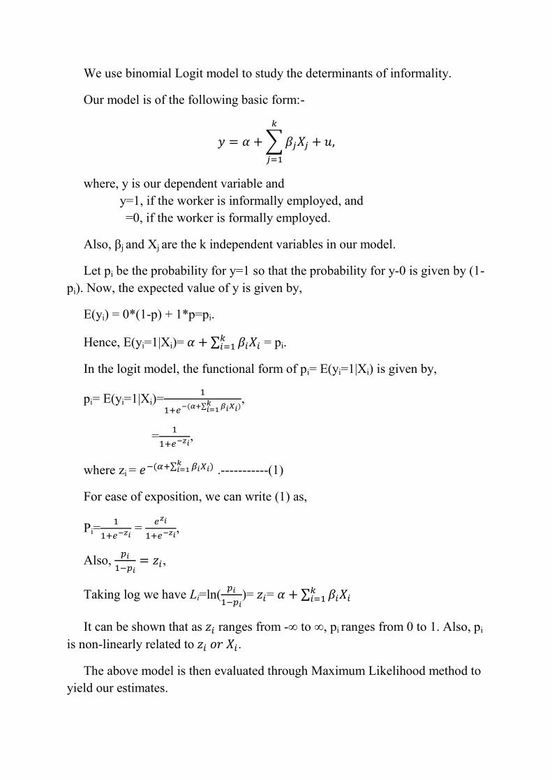
We use binomial Logit model to study the determinants of informality.
Our model is of the following basic form:-
∑
where, y is our dependent variable and
y=1, if the worker is informally employed, and
=0, if the worker is formally employed.
Also, βj and Xj are the k independent variables in our model.
Let pi be the probability for y=1 so that the probability for y-0 is given by (1-
pi). Now, the expected value of y is given by,
E(yi) = 0*(1-p) + 1*p=pi.
Hence, E(yi=1|Xi)= ∑ = pi.
In the logit model, the functional form of pi= E(yi=1|Xi) is given by,
pi= E(yi=1|Xi)=
∑
,
=
,
where zi = ∑ .-----------(1)
For ease of exposition, we can write (1) as,
Pi=
=
,
Also,
,
Taking log we have Li=ln(
)= = ∑
It can be shown that as ranges from -∞ to ∞, pi ranges from 0 to 1. Also, pi
is non-linearly related to .
The above model is then evaluated through Maximum Likelihood method to
yield our estimates.
The literature suggests a number of determinants of informality among them
being age, years of education, technical education, household income, religion,
social group, gender, marital status, sector and industry (Bairagya, 2012;
Henley, Arabsheibani, & Carneiro, 2009; Yu, 2012). We consider the impact of
these variables on informality in our model. We include both age and its square
in our model as we hypothesize a quadratic relation of age with informality.
However, taking both age and its square creates the problem with
multicollinearity. Hence, we deduct from age its mean and take the demean age
and its square in our model which solves our multicollinearity problem.
Similarly, in order to bring out the effect of education we utilise the information
on the education status of workers. However, rather than taking dummies for
different educational levels we derive a continuous variable depicting the mean
years of education of the workers. The methodology used to arrive at this
variable is discussed in the Appendix II to the paper. In order to capture the
effect of technical education on informality, we take a dummy for the presence
or absence of technical education in our model. Monthly Per Capita
Consumption Expenditure (MPCE) of the household is taken as a proxy for
household income in our model. Rather than taking absolute MPCE levels, we
take the natural logarithm of MPCE in our model as it helps to reduce the scale
and dispersion of the variable and makes it normally distributed. We also look
at the incidence of poverty across various poverty groups. The derivation of
poverty groups is discussed in the Appendix III to the paper.
Among the socio-economics variables included in our model are religion and
social group. We consider three broad religions for our study- Hindu, Islam and
„Others‟ which includes all other religions. We include separate dummies for all
the religions except Hindus which we take as the reference category. Similarly,
we create separate dummies for the social groups excluding „Others‟ which we
consider as the reference category. We also have separate dummies for gender
(male/female) and sector (rural/urban) our study. We interpret our results taking
females and urban as the reference categories respectively. Similarly, for marital
status we divide the workforce into two groups- never married and married
where all currently married, divorced and widowed workers are clubbed
together into a single category. We interpret our results against the base
category of never married workers. Finally, we also include dummies for the
industrial affiliation of the workers. The industrial affiliation of the workers can
be obtained from the National Industrial Classification (NIC) code of the
respective workers available in the NSSO data. We divide workers into 7 broad
industries viz. „Agriculture‟ (excluding Cultivation workers); „Mining,
Electricity & Water Supply‟; „Manufacturing‟; „Construction‟; „Trade, Hotels &
Transportation‟; and „Finance, Insurance & Real Estate‟. We create separate
dummies for all the above industries except for „Trade, Hotels &
Transportation‟ which we consider as our reference category.
Finally, we examine the determinants of informality at the macro level
using panel econometrics. The incidence of informality across states is
measured by the proportion of the non-cultivation workforce informally
employed in each state. We use various macro level variables as determinants of
informality across states. In doing so, the study makes an attempt to examine
the strength of alternative hypotheses of different schools of thought in
explaining the occurrence of informality in the country. Similar studies have
tried to study the relative weight of alternative theories in explaining the cross-
country variation in informality(Hazans, 2011; ILO, 2012; Perry et al., 2010;
Williams, 2013, 2015). These studies have found do not favour any particular
hypothesis but find multiple factors driving informality. The various macro
level variables used in our study are discussed below:-
a. In order to examine the argument of the dualist school that informality
is associated with high poverty and underdevelopment, we consider
per capita Gross State Domestic Product (GSDP) as well as Poverty
rates at the state level.
b. In order to examine the soundness of the neo-liberal school that
informality is associated with burdensome governmental regulations
and taxes, we take into account the Tax-GSDP ratio of the state.
c. Similarly, the validity of the structuralist view of rising informality
associated with lower governmental intervention is examined taking
into consideration the Expenditure-GSDP ratio of the state.
d. Lastly, we also consider the state level Gini co-efficient, last 3-year
growth rate as well as an index of government quality to measure the
impact of inequality, growth and quality of public services
respectively on informality rates.
We collect data on all the variables for the years 2004-05 and 2011-12. We
have excluded the Union Territories from our analysis. We also merge the six
geographically contagious North-Eastern states of Manipur, Meghalaya,
Mizoram, Nagaland, Sikkim and Arunachal Pradesh as these states have
individually small sample sizes. In all we have data on 23 state regions for two
time periods. The calculation of the different variables used in our macro study
is discussed in Appendix IV. Finally, we discuss our panel econometric
methodology:-
Breusch-Pagan test as well as Hausman test applied on our model suggests
that fixed-effects model would be appropriate for our data. Our fixed-effects
panel data model is then given by,
∑ ------------(2)
where, i indexes individuals, t indexes time periods and βj‟s and Xj‟s are the
k independent variables in our model.
In the fixed effects model, we allow the intercept term to vary across
individuals so that would capture the unobserved heterogeneity across
individuals. Also, we allow to be correlated with the . Averaging (2) over
time yields,
∑ ------------(3)
Subtracting (3) from (2), we get,
∑
-----------(4)
The individual-specific effects captured by terms cancel each other as
they are invariant over time. Applying OLS to the final model in (3), we arrive
at our fixed-effects estimates.
3. RESULTS AND DISCUSSION
A. TRENDS OF INFORMALITY
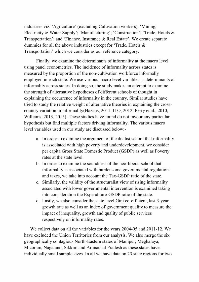
We first take a look at the overall rates of informality in the country-
Table 1: Labour Informality in India
2004-05 2011-12 Formal Informal Total Formal Informal Total
Organised 49.93 50.07 24.82 43.05 56.95 31.58
Unorganised 1.01 98.99 75.18 1.57 98.43 68.42 Total 13.15 86.85 100 14.68 85.32 100
Source: Authors’ calculation based on NSSO data
Labour Informality seems to be quite high in the Indian scenario with
around 87 per cent of the non-cultivation workers being employed under
informal working conditions in 2004-05. Although this figure fell to around 85
per cent in 2011-12, labour informality is still significant. Similarly, percentage
of non-cultivation workers working in the unorganized sector is also substantial
at 75 per cent in 2004-05 which fell down significantly to 68 per cent in 2011-
12. Looking at the composition of employment within the organised sector, we
find that around half of the organised sector workers are informally employed in
2004-05, a figure which rose to 57 per cent in 2011-12. These figures highlight
the rising informalisation of the workforce within the formal sector. Although,
the proportion of unorganised sector workers engaged informally is
insignificant at around 6 per cent in 2004-05, it still rose slightly to around 7 per
cent in 2011-12. (Table 1)
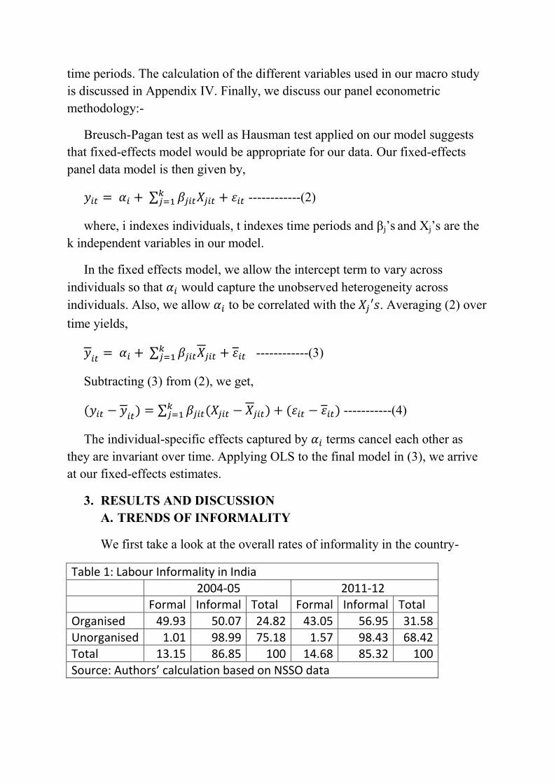
Table 2: Informality across Usual Status Year 2004-05 2011-12
Usual Status Formal Informal Formal Informal Own-account workers 0 100 0 100
Employers 13.98 86.02 12.99 87.01
Unpaid family worker 0 100 0 100 Regular Workers 43.97 56.03 44.32 55.68
Casual Workers (Public Works)
4.02 95.98 1.87 98.13
Casual Workers (Other Works)
1.39 98.61 1.21 98.79
Total 13.15 86.85 14.68 85.32 Source: Authors’ calculation based on NSSO data
If we look at the composition of informality across usual status we find
that own-account employees, unpaid family workers and casual workers consist
entirely of the informally employed in both the periods. Around 87 per cent of
the self-employed employers are informally employed, whereas around 55 per
cent of the regular workers are informally employed. The picture is similar for
2011-12 with no significant changes in the rates of informality. (Table 2)
Table 3: Informality across educational levels
2004-05 2011-12
Years of Education Formal Informal Formal Informal
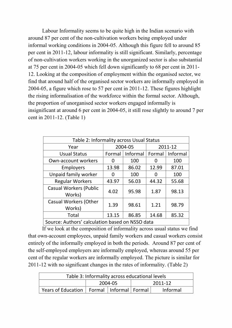
Below 6 Years 3.74 96.26 3.41 96.59
6 to 12 Years 15.06 84.94 13.11 86.89 13 Years & above 46.1 53.9 48.86 51.14
Total 13.15 86.85 14.68 85.32 Source: Authors’ calculation based on NSSO data
Table 4: Informality across Technical Education Year 2004-05 2011-12
Technical Education
Formal Informal Formal Informal
Have 47.58 52.42 55.37 44.63 Don’t Have 11.36 88.64 12.54 87.46
Total 13.15 86.85 14.67 85.33
Source: Authors’ calculation based on NSSO data Similarly, the analysis of educational levels of informality can give us
some idea on the skills of the workers in the different groups. Looking across
educational levels, we find the prevalence of informality falling drastically as
one move towards higher educational levels with informality rates falling from
a high of above 95 per cent for those with primary education or below to a low
of around 50 per cent for those with at least a diploma. Over the period, we see
stagnant or rising informality in the lower or intermediate educational levels
whereas informality is seen to fall at the higher educational levels. (Table 3)
Informality is also found to be significantly higher among workers without
technical education. There is also an evident decline in informality among all
workers over the period, especially among those without a technical education.
(Table 4)
Table 5: Informality across Age
Year 2004-05 2011-12 Age Formal Informal Formal Informal
Below 15 0.58 99.42 0.28 99.72 16-25 4.12 95.88 7.86 92.14
26-35 12.12 87.88 14.56 85.44
36-45 18.68 81.32 16.75 83.25 46-60 24.88 75.12 22.61 77.39
61 & above 1.64 98.36 2.66 97.34 Total 13.15 86.85 14.68 85.32
Source: Authors’ calculation based on NSSO data
Next, we try to look at the dynamics of informality across ages. Here, we
may consider age as an amalgam of the on-the-job-skills of the workers, his
experience over the years as well as his social contacts accumulated. Hence, the
relation of informality with age might give us an inkling of the possible
lifecycle dynamics of the workers as workers move between jobs over the
lifetime. The incidence of informality across age groups shows a distinct U-
shaped pattern with informality falling from a high level with rising age before
rising among the elderly. Probing on it further, we find that the U-shaped patter
is evident only for the wage employment category which makes the overall
pattern U-shaped. Hence, we presume that the U-shaped pattern may reflect the
aggregation of the internal heterogeneity within the informal economy. We
hypothesize that informality is higher in lower ages as people queue in the
informal sector for better jobs. As they accumulate skills, experience and
contacts they get employed in the formal sector. However as age rise beyond a
certain point, informality tends to which may reflect the weight of rising
probability of informality among the employers and own-account workers in the
higher ages. The incidence of informality is also found to have declined over the
period across all age groups. (Table 5)
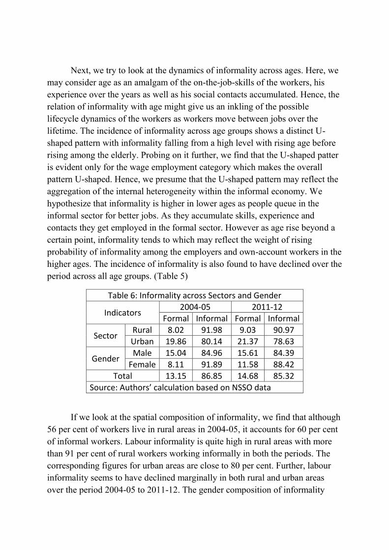
Table 6: Informality across Sectors and Gender
Indicators 2004-05 2011-12
Formal Informal Formal Informal
Sector Rural 8.02 91.98 9.03 90.97 Urban 19.86 80.14 21.37 78.63
Gender Male 15.04 84.96 15.61 84.39
Female 8.11 91.89 11.58 88.42 Total 13.15 86.85 14.68 85.32
Source: Authors’ calculation based on NSSO data
If we look at the spatial composition of informality, we find that although
56 per cent of workers live in rural areas in 2004-05, it accounts for 60 per cent
of informal workers. Labour informality is quite high in rural areas with more
than 91 per cent of rural workers working informally in both the periods. The
corresponding figures for urban areas are close to 80 per cent. Further, labour
informality seems to have declined marginally in both rural and urban areas
over the period 2004-05 to 2011-12. The gender composition of informality
shows that informality among women to be higher than men in both the the
periods. We also see a marginal decline in informality among women, even
though it is more or less stagnant among men. (Table 6)
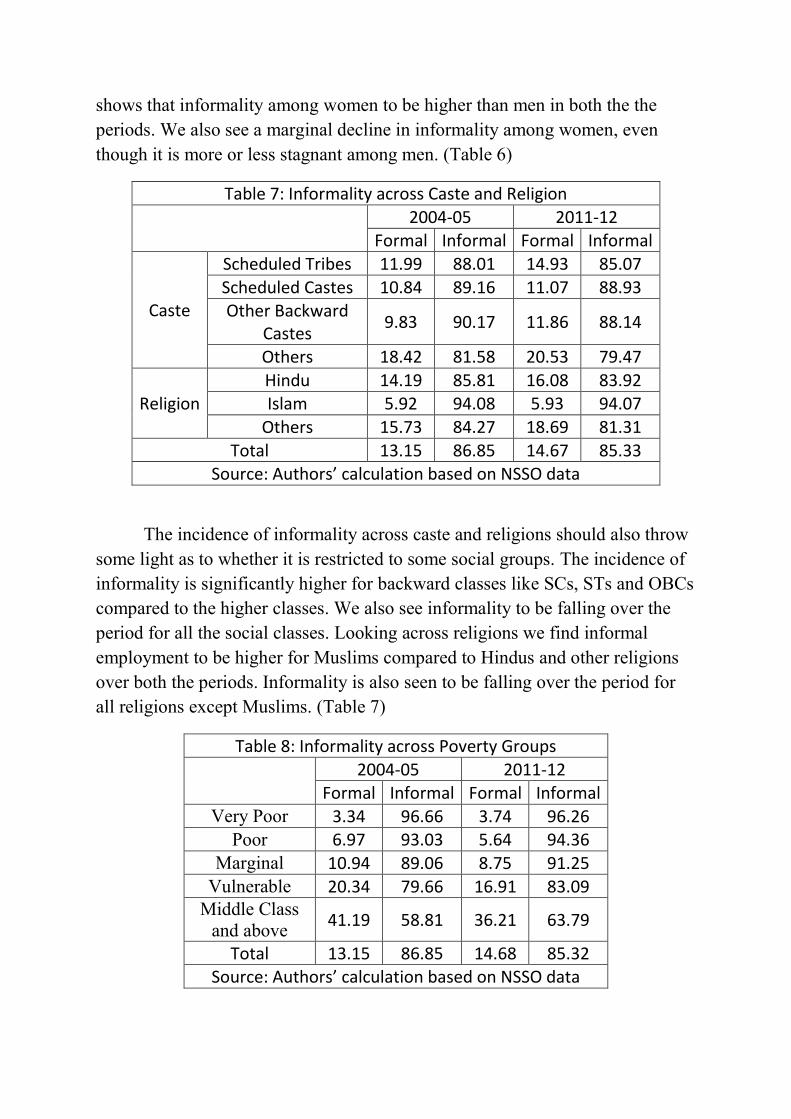
Table 7: Informality across Caste and Religion
2004-05 2011-12
Formal Informal Formal Informal
Caste
Scheduled Tribes 11.99 88.01 14.93 85.07
Scheduled Castes 10.84 89.16 11.07 88.93 Other Backward
Castes 9.83 90.17 11.86 88.14
Others 18.42 81.58 20.53 79.47
Religion Hindu 14.19 85.81 16.08 83.92 Islam 5.92 94.08 5.93 94.07
Others 15.73 84.27 18.69 81.31
Total 13.15 86.85 14.67 85.33 Source: Authors’ calculation based on NSSO data
The incidence of informality across caste and religions should also throw
some light as to whether it is restricted to some social groups. The incidence of
informality is significantly higher for backward classes like SCs, STs and OBCs
compared to the higher classes. We also see informality to be falling over the
period for all the social classes. Looking across religions we find informal
employment to be higher for Muslims compared to Hindus and other religions
over both the periods. Informality is also seen to be falling over the period for
all religions except Muslims. (Table 7)
Table 8: Informality across Poverty Groups
2004-05 2011-12
Formal Informal Formal Informal Very Poor 3.34 96.66 3.74 96.26
Poor 6.97 93.03 5.64 94.36 Marginal 10.94 89.06 8.75 91.25
Vulnerable 20.34 79.66 16.91 83.09 Middle Class
and above 41.19 58.81 36.21 63.79
Total 13.15 86.85 14.68 85.32 Source: Authors’ calculation based on NSSO data
Many authors consider informality and poverty as synonymous. On the
other hand, others consider incomes to be significantly higher for informal
workers especially the self-employed relative to the formal economy. Hence,
looking at the poverty rates of the workers across informal categories may give
us some insight into the nature of the sector. The incidence of informality is
seen to fall drastically as we move towards higher income classes in both
periods. However, the incidence of informality is seen to rise marginally over
the period in all MPCE classes except in the lowest group where it is more or
less stagnant. (Table 8)
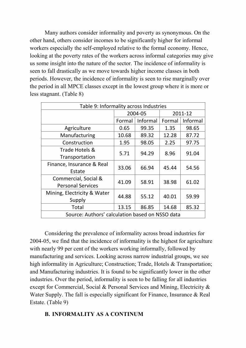
Table 9: Informality across Industries
2004-05 2011-12 Formal Informal Formal Informal
Agriculture 0.65 99.35 1.35 98.65 Manufacturing 10.68 89.32 12.28 87.72
Construction 1.95 98.05 2.25 97.75 Trade Hotels & Transportation
5.71 94.29 8.96 91.04
Finance, Insurance & Real Estate
33.06 66.94 45.44 54.56
Commercial, Social & Personal Services
41.09 58.91 38.98 61.02
Mining, Electricity & Water Supply
44.88 55.12 40.01 59.99
Total 13.15 86.85 14.68 85.32
Source: Authors’ calculation based on NSSO data
Considering the prevalence of informality across broad industries for
2004-05, we find that the incidence of informality is the highest for agriculture
with nearly 99 per cent of the workers working informally, followed by
manufacturing and services. Looking across narrow industrial groups, we see
high informality in Agriculture; Construction; Trade, Hotels & Transportation;
and Manufacturing industries. It is found to be significantly lower in the other
industries. Over the period, informality is seen to be falling for all industries
except for Commercial, Social & Personal Services and Mining, Electricity &
Water Supply. The fall is especially significant for Finance, Insurance & Real
Estate. (Table 9)
B. INFORMALITY AS A CONTINUM
So far we have discussed informality as the presence or absence of
particular work related benefits such as pensions or medical benefits. The
enterprise-based definition which hinges on the size of the enterprise also
divides the workers in a dichotomous scale. However, as discussed earlier,
informality can be seen in a continuous scale of the presence of a number of
considerations such as job contact, location of workplace, eligibility for paid
leave apart from pensions and social security benefits. Considering all these
measures we created a scale of informality which measures the magnitude of
informality so that lower the value in the scale, higher is the informality.
Looking at this informality scale we find that the more informal a worker
is the more likely he is to be working in the unorganised sector. Further, higher
informality is more likely to be associated with women and workers from rural
areas. Interestingly however, totally informal workers are disproportionally
male. Higher informality is also more likely to be associated with lower levels
of education. Further, higher castes and Hindus are considerably more formal
compared to the other groups. Looking across poverty groups, we find that the
more informal groups are markedly more poor compared to the formal groups.
Finally, we find that the informal groups have a significantly younger
workforce. Moreover, these groups also have a sizeable proportion of elderly
among them. The results show that the Informality Continuum Index closely
corresponds with other dichotomous measures of informality.
C. DETERMINANTS OF INFORMALITY
We finally discuss the binomial logit results of our study-
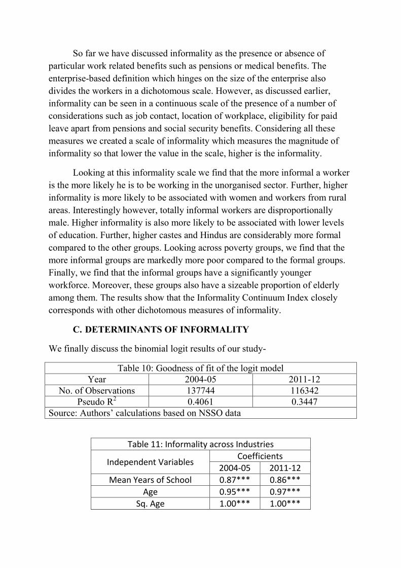
Table 10: Goodness of fit of the logit model
Year 2004-05 2011-12
No. of Observations 137744 116342
Pseudo R2 0.4061 0.3447
Source: Authors‟ calculations based on NSSO data
Table 11: Informality across Industries
Independent Variables Coefficients
2004-05 2011-12
Mean Years of School 0.87*** 0.86***
Age 0.95*** 0.97*** Sq. Age 1.00*** 1.00***
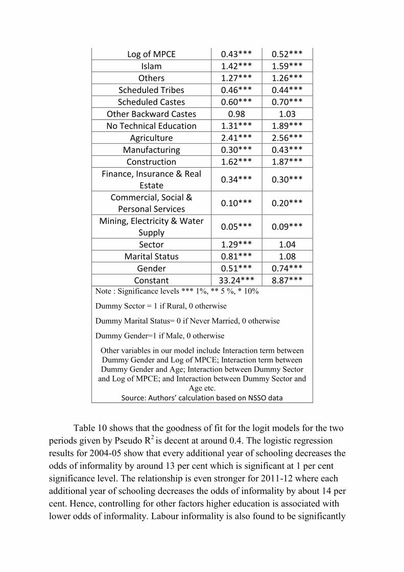
Log of MPCE 0.43*** 0.52***
Islam 1.42*** 1.59*** Others 1.27*** 1.26***
Scheduled Tribes 0.46*** 0.44*** Scheduled Castes 0.60*** 0.70***
Other Backward Castes 0.98 1.03 No Technical Education 1.31*** 1.89***
Agriculture 2.41*** 2.56***
Manufacturing 0.30*** 0.43*** Construction 1.62*** 1.87***
Finance, Insurance & Real Estate
0.34*** 0.30***
Commercial, Social & Personal Services
0.10*** 0.20***
Mining, Electricity & Water Supply
0.05*** 0.09***
Sector 1.29*** 1.04 Marital Status 0.81*** 1.08
Gender 0.51*** 0.74***
Constant 33.24*** 8.87*** Note : Significance levels *** 1%, ** 5 %, * 10%
Dummy Sector = 1 if Rural, 0 otherwise
Dummy Marital Status= 0 if Never Married, 0 otherwise
Dummy Gender=1 if Male, 0 otherwise
Other variables in our model include Interaction term between
Dummy Gender and Log of MPCE; Interaction term between
Dummy Gender and Age; Interaction between Dummy Sector
and Log of MPCE; and Interaction between Dummy Sector and
Age etc. Source: Authors’ calculation based on NSSO data
Table 10 shows that the goodness of fit for the logit models for the two
periods given by Pseudo R2 is decent at around 0.4. The logistic regression
results for 2004-05 show that every additional year of schooling decreases the
odds of informality by around 13 per cent which is significant at 1 per cent
significance level. The relationship is even stronger for 2011-12 where each
additional year of schooling decreases the odds of informality by about 14 per
cent. Hence, controlling for other factors higher education is associated with
lower odds of informality. Labour informality is also found to be significantly
higher for those with no technical education. On average, having no technical
education raises the odds of informality by about 31 per cent and 88 per cent in
2004-05 and 2011-12 respectively. (Table 11)
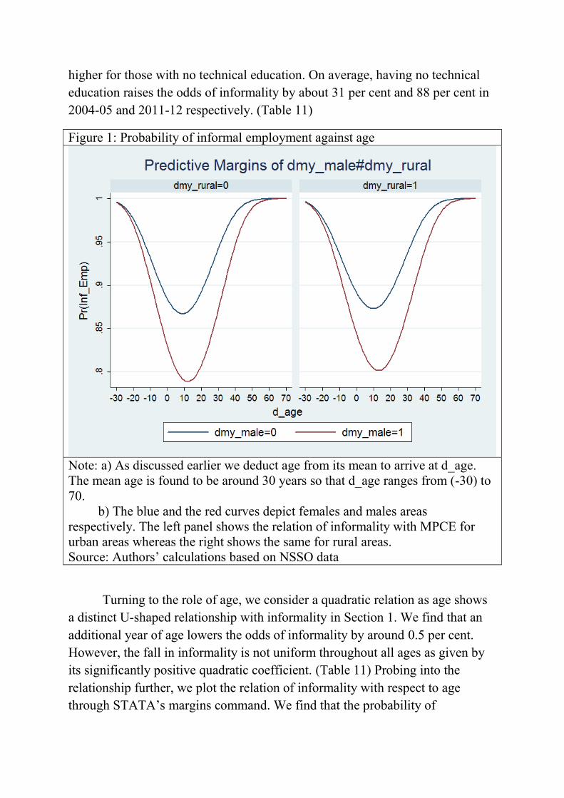
Figure 1: Probability of informal employment against age
Note: a) As discussed earlier we deduct age from its mean to arrive at d_age.
The mean age is found to be around 30 years so that d_age ranges from (-30) to
70.
b) The blue and the red curves depict females and males areas
respectively. The left panel shows the relation of informality with MPCE for
urban areas whereas the right shows the same for rural areas.
Source: Authors‟ calculations based on NSSO data
Turning to the role of age, we consider a quadratic relation as age shows
a distinct U-shaped relationship with informality in Section 1. We find that an
additional year of age lowers the odds of informality by around 0.5 per cent.
However, the fall in informality is not uniform throughout all ages as given by
its significantly positive quadratic coefficient. (Table 11) Probing into the
relationship further, we plot the relation of informality with respect to age
through STATA‟s margins command. We find that the probability of
informality fall from a very high level with increasing age until around the age
of 45 years. Beyond that age, rising age is associated with lower informality.
Looking from a gender perspective, the fall in informality with respect to age is
not much significant for females compared to males. There is not much
difference in the behaviour of informality between rural and urban areas for
both males and females. (Figure 1)
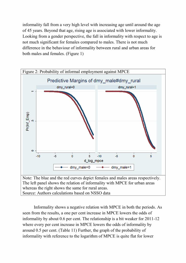
Figure 2: Probability of informal employment against MPCE
Note: The blue and the red curves depict females and males areas respectively.
The left panel shows the relation of informality with MPCE for urban areas
whereas the right shows the same for rural areas.
Source: Authors calculations based on NSSO data
Informality shows a negative relation with MPCE in both the periods. As
seen from the results, a one per cent increase in MPCE lowers the odds of
informality by about 0.6 per cent. The relationship is a bit weaker for 2011-12
where every per cent increase in MPCE lowers the odds of informality by
around 0.5 per cent. (Table 11) Further, the graph of the probability of
informality with reference to the logarithm of MPCE is quite flat for lower
MPCE levels, which becomes steeper as MPCE rises. Hence we postulate that
informality falls marginally with rising MPCE at lower levels of MPCE, but this
relation becomes much steeper at higher MPCE levels. Further, informality is
also found to be higher among females compared to males for all MPCE levels
in both rural and urban areas. (Figure 2)
Looking at informality for different religions, we find that for 2004-05
compared to the reference category of Hindus, informality is higher for Muslims
and Others for both the periods. Comparing across social groups, we see that
informality is significantly lower for STs and SCs against the reference category
of the „Others‟ group. The relationship is not found to be significant in the case
of OBCs. (Table 11)
Further, we find that informality is significantly higher in rural areas
compared to urban areas. For 2004-05, being from a rural area increases the
odds of informality by about 30 per cent. However, this relationship weakens
down considerably for 2011-12, where the coefficient for rural areas is
insignificant. Hence, the odds of informality in rural areas compared to urban
areas have fallen considerably over the period. We similarly find a statistically
significant negative relationship between being male and being informal. Being
male decreases the odds of informality by about 50 per cent and 26 per cent for
2004-05 and 2011-12 respectively. The fall in the coefficient for 2011 implies
falling odds of informality among women over the period. Further, being
married decreases the odds of informality by about 20 per cent in 2004-05.
However, this relation dissipates in 2011-12 as we don‟t find a statistically
significant relationship between informality and being married. (Table 11)
Looking at informality across industries we find that in 2004-05.
Informality is found to be significantly higher in the Agriculture and
Construction industries with reference to the Trade, Hotels & Transportation
industry. Similarly, compared to the base category of Trade, Hotels &
Transportation industry, informality is found to be significantly lower in
Manufacturing; Finance, Insurance & Real Estate; Commercial, Social &
Personal Services as well as Mining, Electricity & Water Supply. The results
are similar for 2011-12. (Table 11)
D. INFORMALITY ACROSS THE STATES
The investigation of the determinants of informality at the individual
level has given us crucial inputs on its nature at the micro level. However, in
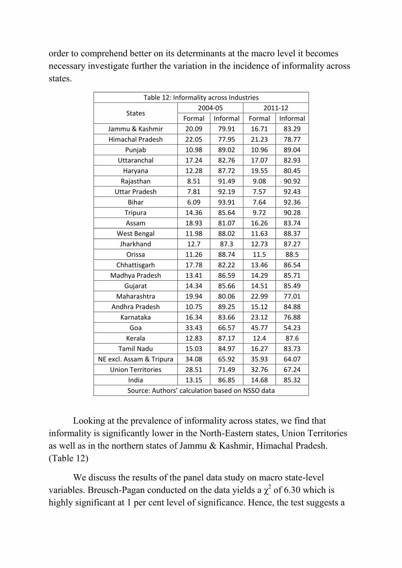
order to comprehend better on its determinants at the macro level it becomes
necessary investigate further the variation in the incidence of informality across
states.
Table 12: Informality across Industries
States 2004-05 2011-12
Formal Informal Formal Informal
Jammu & Kashmir 20.09 79.91 16.71 83.29
Himachal Pradesh 22.05 77.95 21.23 78.77
Punjab 10.98 89.02 10.96 89.04
Uttaranchal 17.24 82.76 17.07 82.93
Haryana 12.28 87.72 19.55 80.45
Rajasthan 8.51 91.49 9.08 90.92
Uttar Pradesh 7.81 92.19 7.57 92.43
Bihar 6.09 93.91 7.64 92.36
Tripura 14.36 85.64 9.72 90.28
Assam 18.93 81.07 16.26 83.74
West Bengal 11.98 88.02 11.63 88.37
Jharkhand 12.7 87.3 12.73 87.27
Orissa 11.26 88.74 11.5 88.5
Chhattisgarh 17.78 82.22 13.46 86.54
Madhya Pradesh 13.41 86.59 14.29 85.71
Gujarat 14.34 85.66 14.51 85.49
Maharashtra 19.94 80.06 22.99 77.01
Andhra Pradesh 10.75 89.25 15.12 84.88
Karnataka 16.34 83.66 23.12 76.88
Goa 33.43 66.57 45.77 54.23
Kerala 12.83 87.17 12.4 87.6
Tamil Nadu 15.03 84.97 16.27 83.73
NE excl. Assam & Tripura 34.08 65.92 35.93 64.07
Union Territories 28.51 71.49 32.76 67.24
India 13.15 86.85 14.68 85.32
Source: Authors’ calculation based on NSSO data
Looking at the prevalence of informality across states, we find that
informality is significantly lower in the North-Eastern states, Union Territories
as well as in the northern states of Jammu & Kashmir, Himachal Pradesh.
(Table 12)
We discuss the results of the panel data study on macro state-level
variables. Breusch-Pagan conducted on the data yields a χ2 of 6.30 which is
highly significant at 1 per cent level of significance. Hence, the test suggests a
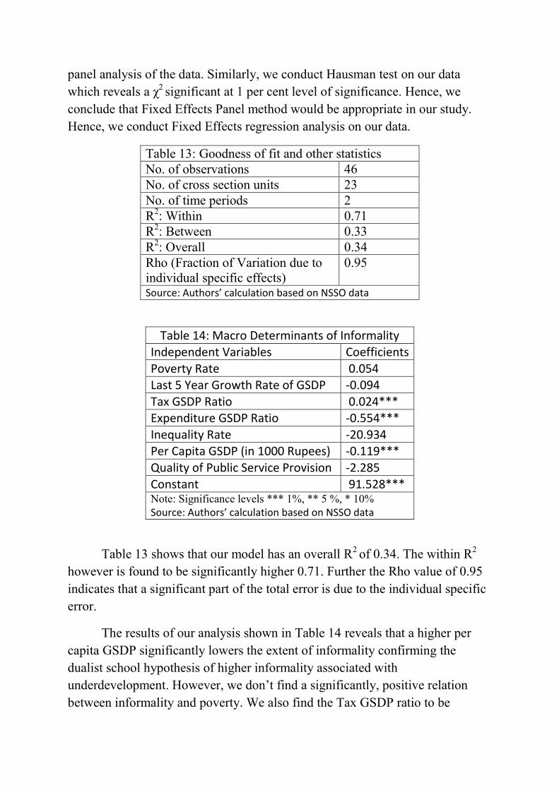
panel analysis of the data. Similarly, we conduct Hausman test on our data
which reveals a χ2 significant at 1 per cent level of significance. Hence, we
conclude that Fixed Effects Panel method would be appropriate in our study.
Hence, we conduct Fixed Effects regression analysis on our data.
Table 13: Goodness of fit and other statistics
No. of observations 46
No. of cross section units 23
No. of time periods 2
R2: Within 0.71
R2: Between 0.33
R2: Overall 0.34
Rho (Fraction of Variation due to
individual specific effects)
0.95
Source: Authors’ calculation based on NSSO data
Table 14: Macro Determinants of Informality
Independent Variables Coefficients
Poverty Rate 0.054 Last 5 Year Growth Rate of GSDP -0.094
Tax GSDP Ratio 0.024*** Expenditure GSDP Ratio -0.554***
Inequality Rate -20.934 Per Capita GSDP (in 1000 Rupees) -0.119***
Quality of Public Service Provision -2.285
Constant 91.528*** Note: Significance levels *** 1%, ** 5 %, * 10%
Source: Authors’ calculation based on NSSO data
Table 13 shows that our model has an overall R2 of 0.34. The within R
2
however is found to be significantly higher 0.71. Further the Rho value of 0.95
indicates that a significant part of the total error is due to the individual specific
error.
The results of our analysis shown in Table 14 reveals that a higher per
capita GSDP significantly lowers the extent of informality confirming the
dualist school hypothesis of higher informality associated with
underdevelopment. However, we don‟t find a significantly, positive relation
between informality and poverty. We also find the Tax GSDP ratio to be
positively related to informality at 1 per cent level of significance. This
vindicates the neo-liberal hypothesis of informality rising with higher
government taxes and regulations. Similarly, Expenditure GSDP ratio is also
found to have a significantly positive relation with informality rates. This result
favours the structuralist view that informality is rising due to falling
governmental presence to protect workers from poverty. However, other
independent factors such as inequality rate, growth as well quality of public
services is not found to have any significant impact on informality. On the
whole, our results shows that informality is not driven by any single set of
macro factors but rather there are multiple factors leading to its rising incidence.
4. CONCLUSION
The study makes an attempt to examine the trends and determinants of
informality in India. The paper finds informality to be significantly higher
among the illiterates, youth, females and the poor. It also finds informality to be
lower among the Hindus, STs and SCs. Its incidence is also found to be higher
in Agriculture and Construction relative to other industries. Although rural
dwellers and the married are found to be significantly more prone to be informal
in 2004-05, this relation dissipates in 2011-12.
The paper also finds informality to be driven by a multitude of
macroeconomic factors such as per capita incomes, tax-GDP ratio as well as
expenditure-GSDP ratio highlighting the significance of different schools of
thought in explaining the phenomenon. Hence, we conclude that efforts to
reduce the incidence of informality would need a multi-pronged strategy rather
than working on a single front.
REFERENCES
ILO. (2004). Economic Security for a Better World (1st ed.). Geneva: ILO. Retrieved from:
http://www.social-
protection.org/gimi/gess/RessourcePDF.action;jsessionid=ba5695c9f7bbc9a3a30c5d398
728626619fcdcfb08ee9b6437707cd5e3e60929.e3aTbhuLbNmSe34MchaRahaKch90?re
ssource.ressourceId=8670
Chen, M. A. (2012). The Informal Economy : Definitions , Theories and Policies.
Chen, M., Vanek, J., Lund, F., Heintz, J., & Christine, J. (2005). PROGRESS OF THE WORLD ’ S
WOMEN WOMEN WORK & POVERTY.
Hazans, M. (2011). What Explains Prevalence of Informal Employment in What Explains Prevalence
of Informal Employment in European Countries: The Role of Labor Institutions , Governance,
Immigrants, and Growth. IZA Discussion Papers, (5872).
ILO. (2012). Statistical update on employment in the informal economy, (June).
Jütting, J., Parlevliet, J., & Xenogiani, T. (2008). Informal Employment Re-loaded DEVELOPMENT
CENTRE WORKING PAPERS.
Maloney, W. F. (2004). Informality revisited. World Development, 32(7), 1159–1178.
http://doi.org/10.1016/j.worlddev.2004.01.008
Oviedo, A., Thomas, M., & Karakurum-Özdemir, K. (2009). Economic informality: causes, costs, and
policies: a literature survey. Retrieved from http://www-
wds.worldbank.org/external/default/WDSContentServer/WDSP/IB/2009/09/16/000333037_200
90916010012/Rendered/PDF/503600PUB0Box3101OFFICIAL0USE0ONLY1.pdf
Perry, G. E., Maloney, W. F., Arias, O. S., Fajnzylber, P., & Saavedra-chanduvi, A. D. M. J. (2010).
Exit and Exclusion. World (Vol. 57). http://doi.org/10.1596/978-0-8213-7092-6
Williams, C. C. (2013). Evaluating cross-national variations in the extent and nature of informal
employment in the European Union. Industrial Relations Journal, n/a–n/a.
http://doi.org/10.1111/irj.12030
Williams, C. C. (2015). Cross-national variations in the scale of informal employment. International
Journal of Manpower, 36(2), 118–135. http://doi.org/10.1108/IJM-01-2014-0021
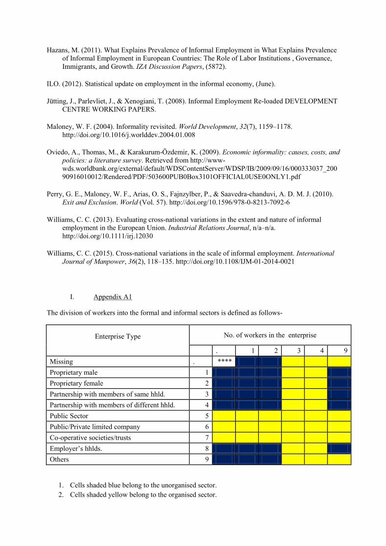
I. Appendix A1
The division of workers into the formal and informal sectors is defined as follows-
Enterprise Type
No. of workers in the enterprise
. 1 2 3 4 9
Missing . ****
Proprietary male 1
Proprietary female 2
Partnership with members of same hhld. 3
Partnership with members of different hhld. 4
Public Sector 5
Public/Private limited company 6
Co-operative societies/trusts 7
Employer‟s hhlds. 8
Others 9
1. Cells shaded blue belong to the unorganised sector.
2. Cells shaded yellow belong to the organised sector.
3. Cells marked with * belongs to the informal sector for all Usual Status except regular and
casual workers in government works. Casual workers in public works belong to the organised
sector. Similarly, Regular workers belong to the informal sectors if they have Social Security
benefits or information on the variable is missing.
The division of workers into the formal and informal employment is done on the basis of
presence of social security benefits and informal sector status as follows-
1. Own account workers and unpaid family workers as categorised into informal employment.
2. Casual workers in public works and other works as well as Regular workers are categorised
into the formal or informal employment based on the presence or absence of social security
benefits.
3. Employers are categorised into formal or informal employment based on whether they belong
to the organised or unorganised sector.
II. Appendix A2
The general educational level of a worker is coded as follows in the NSSO data-
not literate -01, literate without formal schooling: EGS/ NFEC/ AEC -02, TLC -03, others -04;
literate: below primary -05, primary -06, middle -07, secondary -08, higher secondary -10,
diploma/certificate course -11, graduate -12, postgraduate and above -13
The above Education levels refer to the highest level successfully completed. For example, if
a person has failed in his graduate examination, then his level will be treated only as „higher
secondary‟. This is the method followed by NSS.
We derive the mean level of education for a worker as follows-
a. All persons for who code for education level are from 01 will be allotted 0 years of
schooling.
b. All persons for who code for education level are from 02 to 04 will be allotted 1 year of
schooling.
c. All persons for whom code for education level is 05 will be allotted 2 years of schooling.
Below primary means up to Std. 4 (max), so we assume that persons falling under this
category will have on an average 2 years of schooling.
d. All persons for whom code for education level is 06 will be allotted 5 years of schooling.
e. All persons for whom code for education level is 07 will be allotted 8 years of schooling.
f. All persons for whom code for education level is 08 will be allotted 10 years of schooling.
g. All persons for whom code for education level is 10 will be allotted 12 years of schooling.
h. All persons for whom code for education level is 11 will be allotted 14 years of schooling.
Diploma courses are usually for 2 years after completion of Std. 12, so we assume that
persons falling under this category will have 14 years of schooling.
i. All persons for whom code for education level is 12 will be allotted 15 years of schooling.
Graduate courses are usually for 3 years after completion of Std. 12, so we assume that
persons falling under this category will have 15 years of schooling.
j. All persons for whom code for education level is 14 will be allotted 17 years of schooling.
Postgraduate courses are usually for 2 years after completion of Graduate programme, so
we assume that persons falling under this category will have 17 years of schooling.
III. APPENDIX A3
Our poverty lines are based on the Rangarajan Committee methodology for the year 2011-12.
For 2004-05 we deflate the poverty lines from the 2011-12 poverty lines for rural and urban areas
using Consumer Price Index for Agricultural Workers and Consumer Price Index for Industrial
Workers respectively. We borrow the methodology proposed by Sengupta, Kannan & Raveendran
(2008) in classifying households into various poverty categories. Our poverty categories are given as
follows-
Poverty Category Criterion
Very Poor If MPCE <= 0.75 times poverty line (PL)
Poor If 0.75 < MPCE <= 1 PL
Marginal If 1 PL < MPCE <= 1.25 PL
Vulnerable If 1.25 PL < MPCE <= 2 PL
Middle Class and above If MPCE > 2 PL
It is worth noting that our poverty rates do not coincide with the Rangarajan
Committee Report as our poverty rates are based on the Consumer Expenditure
information from the Employment-Unemployment Survey rather than Consumer
Expenditure Survey data of NSSO as is the norm. Since consumer expenditure derived
from the latter is always greater than that obtained from the former, our poverty rates are
likely to be larger than the Rangarajan Committee poverty rates.
IV. Appendix A4
The computation of the different variables used in our study is discussed as follows:-
i. For calculation of GSDP per capita we divide GSDP at constant prices of the
particular state by its population.
ii. Calculation of the poverty rates of different states have used the official state level
poverty rates given by the Tendulkar methodology.
iii. In order to calculate the tax-GSDP ratio and the expenditure-GSDP ratio we divide
the total tax revenue and total expenditure of the state by its GSDP at current prices to
arrive at the figures the tax-GSDP ratio and the expenditure-GSDP ratio respectively.
iv. For calculating the inequality rate we have used the Lorenz ratio (or Gini coefficient)
available from NSSO Reports. Since, these figures are available for rural and urban
areas separately we multiply the rural and urban figures by the appropriate rural and
urban population weights to arrive at the inequality rate for a particular state.
v. Calculation of growth rates for the last 5-year period uses the following formula:-
gt=(yt-yt-5)/yt,
where yt is GSDP for year t and yt-5 is the GSDP 5 years earlier.
vi. In order to calculate the index for quality of public services we have used three
broad indicators for Crime, Road and Electricity Infrastructure. For the
calculation of Road Infrastructure Index we have divided the Total Surfaced
Roads of a state by its respective population. Similarly, for Electricity
Infrastructure Index we have used Peak Power Deficit measure for the particular
state. Finally for calculating the Crime Index we have used various measures
such as Rate of IPC Crimes, Rate of Violent Crimes, Rate of Cases Completed by
Police and Percentage of cases completed by Courts in 0-3 years. We normalize
the variable by using the formula-

Normalized Value = (Max. Value - Actual Value) / (Max. Value - Min. Value),
for positive indicators like Roads per population, Rate of cases completed by
police and courts etc.
= (Actual Value – Min. Value) / (Max. Value - Min. Value),
for negative values like Rate of IPC and Violent crimes, Peak Power deficit etc.
We take simple Arithmetic Mean of the indicators of Crime to arrive at
our Crime index. Finally, simple Arithmetic Mean of the Crime Index, Road and
Electricity Infrastructure yields us the Index for Quality of Public Services.
Related Documents