Multivariate Statistics in Ecology and Quantitative Genetics Redundancy analysis Dirk Metzler & Martin Hutzenthaler http://evol.bio.lmu.de/_statgen Summer semester 2011

Welcome message from author
This document is posted to help you gain knowledge. Please leave a comment to let me know what you think about it! Share it to your friends and learn new things together.
Transcript
Multivariate Statistics in Ecology andQuantitative Genetics
Redundancy analysis
Dirk Metzler & Martin Hutzenthaler
http://evol.bio.lmu.de/_statgen
Summer semester 2011
1 Redundancy analysisSettingExample: Artificial fish dataTriplotsExample: Height weight dataExample: Species richness on sandy beaches (RIKZ data)The order of importance
Redundancy analysis Setting
Contents
1 Redundancy analysisSettingExample: Artificial fish dataTriplotsExample: Height weight dataExample: Species richness on sandy beaches (RIKZ data)The order of importance
Redundancy analysis Setting
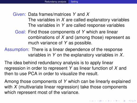
Given: Data frames/matrices Y and XThe variables in X are called explanatory variablesThe variables in Y are called response variables
Goal: Find those components of Y which are linearcombinations of X and (among those) represent asmuch variance of Y as possible.
Assumption: There is a linear dependence of the responsevariables in Y on the explanatory variables in X .
The idea behind redundancy analysis is to apply linearregression in order to represent Y as linear function of X andthen to use PCA in order to visualize the result.
Among those components of Y which can be linearly explainedwith X (multivariate linear regression) take those componentswhich represent most of the variance.
Redundancy analysis Setting
Before applying RDA:
Is Y increasing with increasing values of X?If the variables in X are twice as high, are the variables in Yalso approximately twice as high?
These questions are to check the assumption of lineardependence.

Redundancy analysis Example: Artificial fish data
Contents
1 Redundancy analysisSettingExample: Artificial fish dataTriplotsExample: Height weight dataExample: Species richness on sandy beaches (RIKZ data)The order of importance
Redundancy analysis Example: Artificial fish data
To illustrate the output of redundancy analysis (RDA)we consider an artificial example from p. 590 of
P. Legendre and L. Legendre.Numerical Ecology
(We will not go into the maths of RDA)
Redundancy analysis Example: Artificial fish data
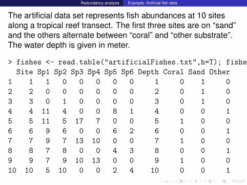
The artificial data set represents fish abundances at 10 sitesalong a tropical reef transect. The first three sites are on “sand”and the others alternate between “coral” and “other substrate”.The water depth is given in meter.
> fishes <- read.table("artificialFishes.txt",h=T); fishes
Site Sp1 Sp2 Sp3 Sp4 Sp5 Sp6 Depth Coral Sand Other
1 1 1 0 0 0 0 0 1 0 1 0
2 2 0 0 0 0 0 0 2 0 1 0
3 3 0 1 0 0 0 0 3 0 1 0
4 4 11 4 0 0 8 1 4 0 0 1
5 5 11 5 17 7 0 0 5 1 0 0
6 6 9 6 0 0 6 2 6 0 0 1
7 7 9 7 13 10 0 0 7 1 0 0
8 8 7 8 0 0 4 3 8 0 0 1
9 9 7 9 10 13 0 0 9 1 0 0
10 10 5 10 0 0 2 4 10 0 0 1
Redundancy analysis Example: Artificial fish data
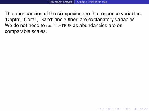
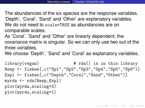
The abundancies of the six species are the response variables.’Depth’, ’Coral’, ’Sand’ and ’Other’ are explanatory variables.We do not need to scale=TRUE as abundancies are oncomparable scales.
As ’Coral’, ’Sand’ and ’Other’ are linearly dependent, thecovariance matrix is singular. So we can only use two out of thethree variables.We choose ’Depth’, ’Sand’ and ’Coral’ as explanatory variables.
library(vegan) # rda() is in this library
Resp <- fishes[,c("Sp1","Sp2","Sp3","Sp4","Sp5","Sp6")]
Expl <- fishes[,c("Depth","Coral","Sand","Other")]
myrda <- rda(Resp,Expl)
plot(myrda,scaling=2)
plot(myrda,scaling=1)
Redundancy analysis Example: Artificial fish data
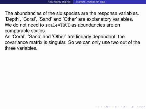
The abundancies of the six species are the response variables.’Depth’, ’Coral’, ’Sand’ and ’Other’ are explanatory variables.We do not need to scale=TRUE as abundancies are oncomparable scales.As ’Coral’, ’Sand’ and ’Other’ are linearly dependent, thecovariance matrix is singular. So we can only use two out of thethree variables.
We choose ’Depth’, ’Sand’ and ’Coral’ as explanatory variables.
library(vegan) # rda() is in this library
Resp <- fishes[,c("Sp1","Sp2","Sp3","Sp4","Sp5","Sp6")]
Expl <- fishes[,c("Depth","Coral","Sand","Other")]
myrda <- rda(Resp,Expl)
plot(myrda,scaling=2)
plot(myrda,scaling=1)
Redundancy analysis Example: Artificial fish data
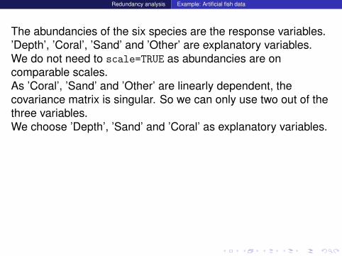
The abundancies of the six species are the response variables.’Depth’, ’Coral’, ’Sand’ and ’Other’ are explanatory variables.We do not need to scale=TRUE as abundancies are oncomparable scales.As ’Coral’, ’Sand’ and ’Other’ are linearly dependent, thecovariance matrix is singular. So we can only use two out of thethree variables.We choose ’Depth’, ’Sand’ and ’Coral’ as explanatory variables.
library(vegan) # rda() is in this library
Resp <- fishes[,c("Sp1","Sp2","Sp3","Sp4","Sp5","Sp6")]
Expl <- fishes[,c("Depth","Coral","Sand","Other")]
myrda <- rda(Resp,Expl)
plot(myrda,scaling=2)
plot(myrda,scaling=1)
Redundancy analysis Example: Artificial fish data
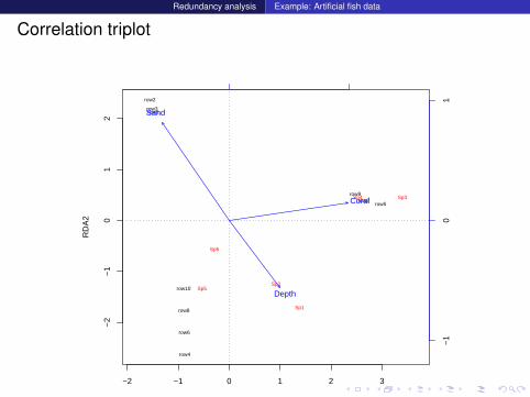
Correlation triplot
−2 −1 0 1 2 3
−2
−1
01
2
RDA1
RD
A2
Sp1
Sp2
Sp3Sp4
Sp5
Sp6
row1
row2
row3
row4
row5
row6
row7
row8
row9
row10Depth
Coral
Sand
−1
01
Redundancy analysis Example: Artificial fish data
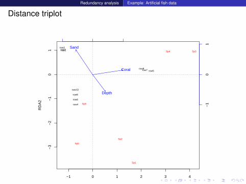
Distance triplot
−1 0 1 2 3 4
−3
−2
−1
01
RDA1
RD
A2
Sp1
Sp2
Sp3Sp4
Sp5
Sp6
row1row2row3
row4
row5
row6
row7
row8
row9
row10
Depth
Coral
Sand
−1
01
Redundancy analysis Example: Artificial fish data
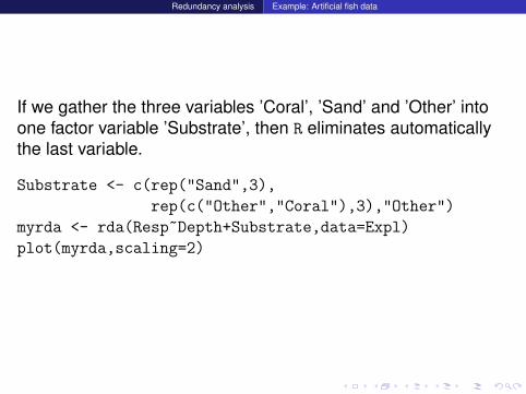
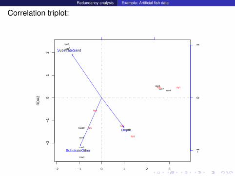
If we gather the three variables ’Coral’, ’Sand’ and ’Other’ intoone factor variable ’Substrate’, then R eliminates automaticallythe last variable.
Substrate <- c(rep("Sand",3),
rep(c("Other","Coral"),3),"Other")
myrda <- rda(Resp~Depth+Substrate,data=Expl)
plot(myrda,scaling=2)
Redundancy analysis Example: Artificial fish data
Correlation triplot:
−2 −1 0 1 2 3
−2
−1
01
2
RDA1
RD
A2
Sp1
Sp2
Sp3Sp4
Sp5
Sp6
row1
row2
row3
row4
row5
row6
row7
row8
row9
row10Depth
SubstrateOther
SubstrateSand
−1
01
Redundancy analysis Triplots
Contents
1 Redundancy analysisSettingExample: Artificial fish dataTriplotsExample: Height weight dataExample: Species richness on sandy beaches (RIKZ data)The order of importance

Redundancy analysis Triplots
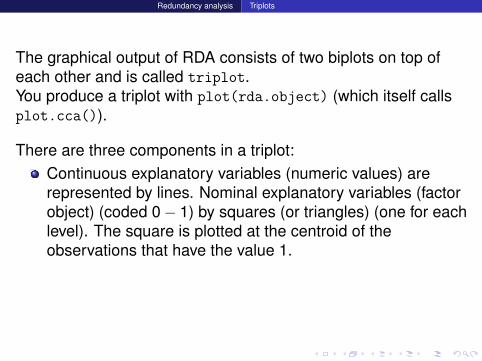
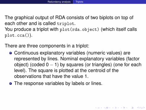
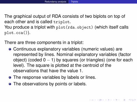
The graphical output of RDA consists of two biplots on top ofeach other and is called triplot.You produce a triplot with plot(rda.object) (which itself callsplot.cca()).
There are three components in a triplot:Continuous explanatory variables (numeric values) arerepresented by lines. Nominal explanatory variables (factorobject) (coded 0 − 1) by squares (or triangles) (one for eachlevel). The square is plotted at the centroid of theobservations that have the value 1.The response variables by labels or lines.The observations by points or labels.
Redundancy analysis Triplots
The graphical output of RDA consists of two biplots on top ofeach other and is called triplot.You produce a triplot with plot(rda.object) (which itself callsplot.cca()).
There are three components in a triplot:Continuous explanatory variables (numeric values) arerepresented by lines. Nominal explanatory variables (factorobject) (coded 0 − 1) by squares (or triangles) (one for eachlevel). The square is plotted at the centroid of theobservations that have the value 1.
The response variables by labels or lines.The observations by points or labels.
Redundancy analysis Triplots
The graphical output of RDA consists of two biplots on top ofeach other and is called triplot.You produce a triplot with plot(rda.object) (which itself callsplot.cca()).
There are three components in a triplot:Continuous explanatory variables (numeric values) arerepresented by lines. Nominal explanatory variables (factorobject) (coded 0 − 1) by squares (or triangles) (one for eachlevel). The square is plotted at the centroid of theobservations that have the value 1.The response variables by labels or lines.
The observations by points or labels.
Redundancy analysis Triplots
The graphical output of RDA consists of two biplots on top ofeach other and is called triplot.You produce a triplot with plot(rda.object) (which itself callsplot.cca()).
There are three components in a triplot:Continuous explanatory variables (numeric values) arerepresented by lines. Nominal explanatory variables (factorobject) (coded 0 − 1) by squares (or triangles) (one for eachlevel). The square is plotted at the centroid of theobservations that have the value 1.The response variables by labels or lines.The observations by points or labels.
Redundancy analysis Triplots
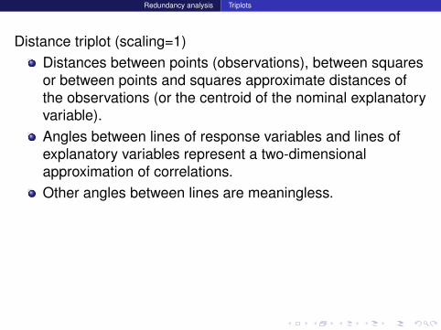
Distance triplot (scaling=1)Distances between points (observations), between squaresor between points and squares approximate distances ofthe observations (or the centroid of the nominal explanatoryvariable).Angles between lines of response variables and lines ofexplanatory variables represent a two-dimensionalapproximation of correlations.Other angles between lines are meaningless.
The projection of a point onto the line of a response variableat right angle approximates the position of thecorresponding object along the corresponding variable.Squares/triangles cannot be compared with lines ofqualitatively explanatory variables.

Redundancy analysis Triplots
Distance triplot (scaling=1)Distances between points (observations), between squaresor between points and squares approximate distances ofthe observations (or the centroid of the nominal explanatoryvariable).Angles between lines of response variables and lines ofexplanatory variables represent a two-dimensionalapproximation of correlations.Other angles between lines are meaningless.The projection of a point onto the line of a response variableat right angle approximates the position of thecorresponding object along the corresponding variable.Squares/triangles cannot be compared with lines ofqualitatively explanatory variables.
Redundancy analysis Triplots
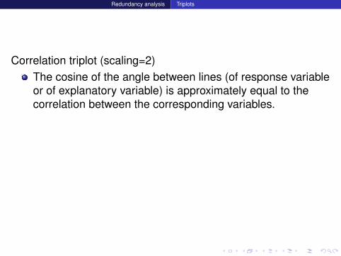
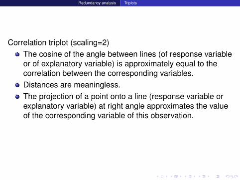
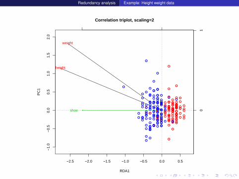
Correlation triplot (scaling=2)The cosine of the angle between lines (of response variableor of explanatory variable) is approximately equal to thecorrelation between the corresponding variables.
Distances are meaningless.The projection of a point onto a line (response variable orexplanatory variable) at right angle approximates the valueof the corresponding variable of this observation.The length of lines are not important.
Redundancy analysis Triplots
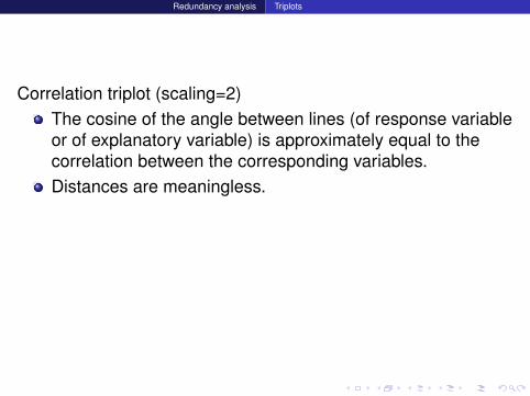
Correlation triplot (scaling=2)The cosine of the angle between lines (of response variableor of explanatory variable) is approximately equal to thecorrelation between the corresponding variables.Distances are meaningless.
The projection of a point onto a line (response variable orexplanatory variable) at right angle approximates the valueof the corresponding variable of this observation.The length of lines are not important.
Redundancy analysis Triplots
Correlation triplot (scaling=2)The cosine of the angle between lines (of response variableor of explanatory variable) is approximately equal to thecorrelation between the corresponding variables.Distances are meaningless.The projection of a point onto a line (response variable orexplanatory variable) at right angle approximates the valueof the corresponding variable of this observation.
The length of lines are not important.
Redundancy analysis Triplots
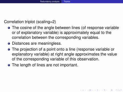
Correlation triplot (scaling=2)The cosine of the angle between lines (of response variableor of explanatory variable) is approximately equal to thecorrelation between the corresponding variables.Distances are meaningless.The projection of a point onto a line (response variable orexplanatory variable) at right angle approximates the valueof the corresponding variable of this observation.The length of lines are not important.
Redundancy analysis Example: Height weight data
Contents
1 Redundancy analysisSettingExample: Artificial fish dataTriplotsExample: Height weight dataExample: Species richness on sandy beaches (RIKZ data)The order of importance

Redundancy analysis Example: Height weight data
Recall hsw and fm.col from the slides on PCA.
Expl <- hsw[,c(1,2,3)]
Resp <- hsw[,c(1,2,3)]
myrda <- rda(Resp~shoe,scale=TRUE,data=Expl)
# Distance triplot
# The following command does not plot (type=None)
plot(myrda,scaling=1,type="n",main="Distance triplot")
segments(x0=0,y0=0,
x1=scores(myrda, display="species", scaling=1)[,1],
y1=scores(myrda, display="species", scaling=1)[,2])
text(myrda, display="sp", scaling=1, col=2)
text(myrda, display="bp", scaling=1,
row.names(scores(myrda, display="bp")), col=3)
points(myrda,display=c("sites"),scaling=1,pch=1,col=fm.col)
Redundancy analysis Example: Height weight data
−4 −3 −2 −1 0 1
−4
−3
−2
−1
0
Distance triplot, scaling=1
RDA1
PC
1
height
shoe
weight
−1
0shoe ●
●●
●
●● ●
●●
●
●●
●●
●
●
●
●●
●
●
●
●●●
●●●
●●
●
●●
●
●
● ●● ●● ●
●●
● ●●
●● ●
●
●
●●
●
●● ●
●
●●●
●●●
●
●●● ●
● ● ●●
●
●
●
●●
●
●●●
●● ●●●
● ●●
●●
● ●
●
●
● ●
●
●
●
● ●
●
●●
●
●●
● ●
●●
●● ●● ●
●●● ●●
●
●
●
●●
●●
●●●
● ● ●●
● ●●●● ●●
● ●●● ●
●
●●
●
●●●
●
●
●●●● ●
●
●
●●●
●
●
●
●●●
●● ●
●●
●
●
●●
●
●
●
●●●
●●●
●
●
● ●●
●
●● ●
●
● ●●●
●
●
●●
●●●
●
●
●
●●
●●
●●
Redundancy analysis Example: Height weight data
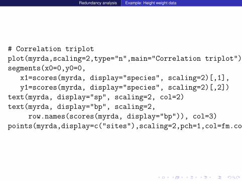
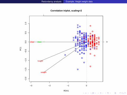
# Correlation triplot
plot(myrda,scaling=2,type="n",main="Correlation triplot")
segments(x0=0,y0=0,
x1=scores(myrda, display="species", scaling=2)[,1],
y1=scores(myrda, display="species", scaling=2)[,2])
text(myrda, display="sp", scaling=2, col=2)
text(myrda, display="bp", scaling=2,
row.names(scores(myrda, display="bp")), col=3)
points(myrda,display=c("sites"),scaling=2,pch=1,col=fm.col)
Redundancy analysis Example: Height weight data
−3 −2 −1 0
−2.
0−
1.5
−1.
0−
0.5
0.0
0.5
1.0
Correlation triplot, scaling=2
RDA1
PC
1
height
shoe
weight
0shoe ●
●
●
●
●●
●
●
●
●
●
●
●
●
●
●
●
●
●
●
●
●
●
●
●
●
●●
●
●
●
●●
●
●
● ●
● ●●
●
●
●
●
●●
●
●
●
●
●
●
●
●
●
●
●
●
●
●
●
●●
●
●
●●
●●
●
●●
●
●
●
●
●
●
●
●●
●
●
●
●●
●
● ●
●
●
●
● ●
●
●
●
●
●
●
●
● ●
●
●
●
●
●
●
● ●
●
●
●
●●
●
●
●
●●
●
●
●
●
●
●
●
●
●
●
●
●
●●
●
●
●
●●
●●
●●
●
●
●●
●
●
●
●
●
●●
●
●
●
●●
●●
●
●
●
●●
●
●
●
●
●
●
●
●
●●
●
●
●
●
●
●
●
●
●
●
●
●
●
●
●
●
●
● ●●
●
●
●●
●
●●●
●
●
●
●
●
●
●●
●
●
●
●
●
●
●
●
●
Redundancy analysis Example: Height weight data
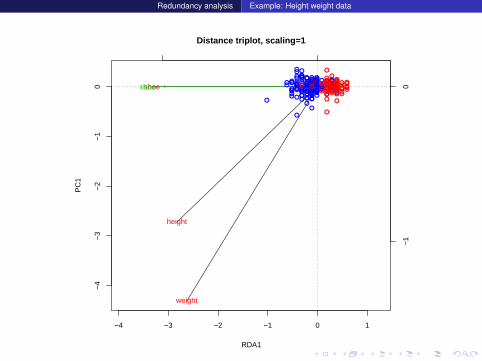
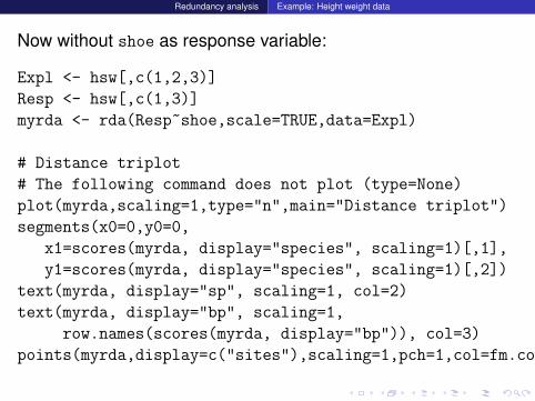
Now without shoe as response variable:
Expl <- hsw[,c(1,2,3)]
Resp <- hsw[,c(1,3)]
myrda <- rda(Resp~shoe,scale=TRUE,data=Expl)
# Distance triplot
# The following command does not plot (type=None)
plot(myrda,scaling=1,type="n",main="Distance triplot")
segments(x0=0,y0=0,
x1=scores(myrda, display="species", scaling=1)[,1],
y1=scores(myrda, display="species", scaling=1)[,2])
text(myrda, display="sp", scaling=1, col=2)
text(myrda, display="bp", scaling=1,
row.names(scores(myrda, display="bp")), col=3)
points(myrda,display=c("sites"),scaling=1,pch=1,col=fm.col)
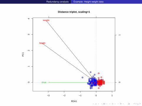
Redundancy analysis Example: Height weight data
−3 −2 −1 0 1
01
23
4
Distance triplot, scaling=1
RDA1
PC
1
height
weight
01
shoe ●
●●
●
●●●
●●
●
●●
●
●
●
●
●
●●
●
●
●
●●●
●●●
●●
●
●●
●
●
● ●● ●● ●
●
●
●●●
●●
●
●
●
●●
●
●● ●
●
●●●
●●
●
●
●●
●●● ● ●●
●
●
●
●
●
●
●●●
●● ●●●
● ●●
●
●●●
●
●
●●
●
●
●
● ●
●
●●
●
●●
●●
●●
●● ●
● ●●●●●●
●
●
●
●●
●
●●●
●● ●
●●
●●●●● ●●
● ●●● ●
●
●●
●
●●
●
●
●
●●●● ●
●
●
●●
●
●
●
●
●●
●●
● ●
●●
●
●
●●
●
●
●
●●●
●●●
●
●
● ●●
●
●●●
●
●●●●
●
●
●●
●●●
●
●
●
●●
●●
●●

Redundancy analysis Example: Height weight data
# Correlation triplot
plot(myrda,scaling=2,type="n",main="Correlation triplot")
segments(x0=0,y0=0,
x1=scores(myrda, display="species", scaling=2)[,1],
y1=scores(myrda, display="species", scaling=2)[,2])
text(myrda, display="sp", scaling=2, col=2)
text(myrda, display="bp", scaling=2,
row.names(scores(myrda, display="bp")), col=3)
points(myrda,display=c("sites"),scaling=2,pch=1,col=fm.col)
Redundancy analysis Example: Height weight data
−2.5 −2.0 −1.5 −1.0 −0.5 0.0 0.5
−1.
0−
0.5
0.0
0.5
1.0
1.5
2.0
Correlation triplot, scaling=2
RDA1
PC
1
height
weight
01
shoe ●
●
●
●
●●
●
●
●
●
●
●
●
●
●
●
●
●
●
●
●
●
●
●
●
●
●●
●
●
●
●●
●
●
● ●
● ●●
●
●
●
●
●●
●
●
●
●
●
●
●
●
●
●●
●
●
●
●
●●
●
●
●●
●●
●
●●
●
●
●
●
●
●
●
●●
●
●
●
●●
●
● ●
●
●
●
● ●
●
●
●
●
●
●
●
● ●
●
●
●
●
●
●
● ●
●
●
●
●●
●
●
●
●●
●
●
●
●
●
●
●
●
●
●
●
●
●●
●
●
●
●●
●●
●●
●
●
●● ●
●
●
●
●
●●
●
●
●
●●
●●
●
●
●
●●
●
●
●
●
●
●
●
●
●●
●
●
●
●
●
●
●
●
●
●
●
●
●
●
●
●
●
● ●●
●
●
●●
●
●●●
●
●
●
●
●
●
●●
●
●
●
●
●
●
●
●
●
Redundancy analysis Example: Species richness on sandy beaches (RIKZ data)
Contents
1 Redundancy analysisSettingExample: Artificial fish dataTriplotsExample: Height weight dataExample: Species richness on sandy beaches (RIKZ data)The order of importance
Redundancy analysis Example: Species richness on sandy beaches (RIKZ data)
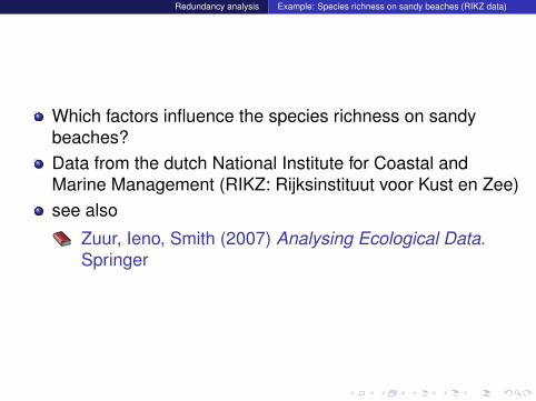
Which factors influence the species richness on sandybeaches?Data from the dutch National Institute for Coastal andMarine Management (RIKZ: Rijksinstituut voor Kust en Zee)see also
Zuur, Ieno, Smith (2007) Analysing Ecological Data.Springer
Redundancy analysis Example: Species richness on sandy beaches (RIKZ data)
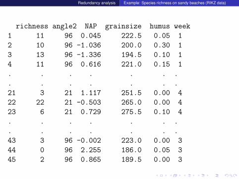
richness angle2 NAP grainsize humus week
1 11 96 0.045 222.5 0.05 1
2 10 96 -1.036 200.0 0.30 1
3 13 96 -1.336 194.5 0.10 1
4 11 96 0.616 221.0 0.15 1
. . . . . . .
. . . . . . .
21 3 21 1.117 251.5 0.00 4
22 22 21 -0.503 265.0 0.00 4
23 6 21 0.729 275.5 0.10 4
. . . . . . .
. . . . . . .
43 3 96 -0.002 223.0 0.00 3
44 0 96 2.255 186.0 0.05 3
45 2 96 0.865 189.5 0.00 3
Redundancy analysis Example: Species richness on sandy beaches (RIKZ data)
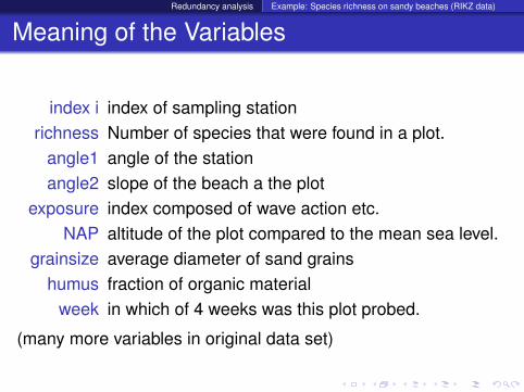
Meaning of the Variables
index i index of sampling stationrichness Number of species that were found in a plot.
angle1 angle of the stationangle2 slope of the beach a the plot
exposure index composed of wave action etc.NAP altitude of the plot compared to the mean sea level.
grainsize average diameter of sand grainshumus fraction of organic material
week in which of 4 weeks was this plot probed.
(many more variables in original data set)
Redundancy analysis Example: Species richness on sandy beaches (RIKZ data)
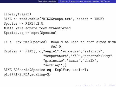
library(vegan)
RIKZ <- read.table("RIKZGroups.txt", header = TRUE)
Species <- RIKZ[,2:5]
#Data were square root transformed
Species.sq <- sqrt(Species)
I1 <- rowSums(Species) #Could be used to drop sites with a total
#of 0.
ExplVar <- RIKZ[, c("angle1","exposure","salinity",
"temperature","NAP","penetrability",
"grainsize","humus","chalk",
"sorting1")]
RIKZ_RDA<-rda(Species.sq, ExplVar, scale=T)
plot(RIKZ_RDA,scaling=2)
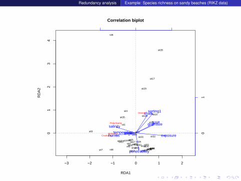
Redundancy analysis Example: Species richness on sandy beaches (RIKZ data)
−3 −2 −1 0 1 2
01
23
4
Correlation biplot
RDA1
RD
A2
Polychaeta
CrustaceaMollusca
Insecta
sit1
sit2sit3
sit4
sit5
sit6
sit7 sit8
sit9
sit10
sit11
sit12sit13
sit14sit15
sit16
sit17
sit18sit19
sit20
sit21
sit22sit23
sit24
sit25sit26sit27
sit28
sit29
sit30sit31
sit32
sit33
sit34
sit35
sit36
sit37
sit38
sit39
sit40
sit41
sit42 sit43
sit44sit45
angle1 exposure
salinity
temperature
NAP
penetrability
grainsize
humus
chalksorting1
01
Redundancy analysis Example: Species richness on sandy beaches (RIKZ data)
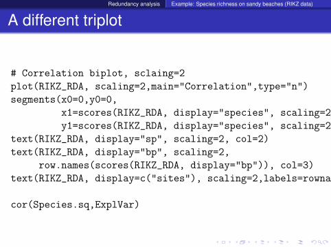
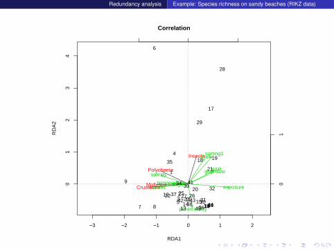
A different triplot
# Correlation biplot, sclaing=2
plot(RIKZ_RDA, scaling=2,main="Correlation",type="n")
segments(x0=0,y0=0,
x1=scores(RIKZ_RDA, display="species", scaling=2)[,1],
y1=scores(RIKZ_RDA, display="species", scaling=2)[,2])
text(RIKZ_RDA, display="sp", scaling=2, col=2)
text(RIKZ_RDA, display="bp", scaling=2,
row.names(scores(RIKZ_RDA, display="bp")), col=3)
text(RIKZ_RDA, display=c("sites"), scaling=2,labels=rownames(Species.sq))
cor(Species.sq,ExplVar)
Redundancy analysis Example: Species richness on sandy beaches (RIKZ data)
−3 −2 −1 0 1 2
01
23
4
Correlation
RDA1
RD
A2
Polychaeta
CrustaceaMollusca
Insecta
01
angle1 exposure
salinity
temperature
NAP
penetrability
grainsize
humus
chalksorting1
1
23
4
5
6
7 8
9
1011
121314 15
16
17
18 19
20
21
2223
24
25 2627
28
29
3031
32
33
34
35
36
37
38
39
40
41
42 4344
45
Redundancy analysis The order of importance
Contents
1 Redundancy analysisSettingExample: Artificial fish dataTriplotsExample: Height weight dataExample: Species richness on sandy beaches (RIKZ data)The order of importance
Redundancy analysis The order of importance
Anova on RDA objects
Which of the explanatory variables is the most important?Which are the least important or even irrelevant?
As RDA is based on linear regression, the same methods apply.Due to time constraint, this is not part of the lecture.
Have a try for yourself:
anova(RIKZ_RDA)
step(RIKZ_RDA)
dropterm(RIKZ_RDA)
Redundancy analysis The order of importance
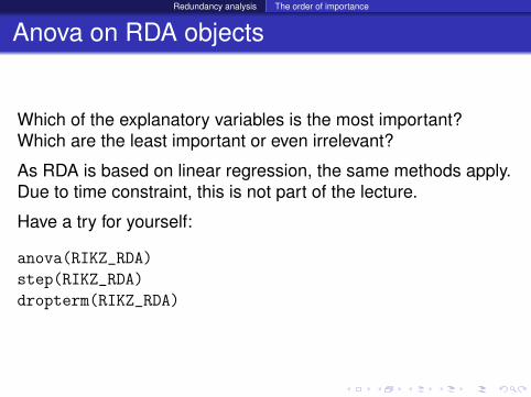
Anova on RDA objects
Which of the explanatory variables is the most important?Which are the least important or even irrelevant?
As RDA is based on linear regression, the same methods apply.Due to time constraint, this is not part of the lecture.
Have a try for yourself:
anova(RIKZ_RDA)
step(RIKZ_RDA)
dropterm(RIKZ_RDA)
Related Documents