Multivariate statistical image processing for molecular specific imaging in organic and bio-systems

Multivariate Statistical Image Processing for Molecular

Specific Imaging in Organic and Bio-systems

Bonnie J. Tyler

Dept. of Chemical Eng., University of Utah, 50 S Central Campus Dr. Rm. 3290, Salt Lake City, Utah 84112, USA

Abstract

Processing TOF-SIMS images to obtain clear contrast between chemically distinct regions,

distinguish between chemical and topographic effects and identify chemical species can be a

formidable challenge, particularly when working with organic and biological molecules that have

similar spectral features. Three multivariate statistical techniques, including principal components

analysis (PCA), multivariate curve resolution (MCR), and maximum auto-correlation factors

(MAF) have been explored to determine their utility for processing TOF-SIMS images. The

methods have been exhaustively tested on synthetic images to allow quantitative assessment of their

utility. The methods are compared here based on enhancement of image contrast, enhancement of

image resolution, and isolation of pure component spectra. MAF, which includes information on the

nearest neighbors to each pixel, shows clear advantages over PCA and MCR for enhancing image

contrast and identifying sparse components in the matrix. However, MCR is better suited to

identification of unknown compounds. No single method proves superior for all of these objectives

so a simple strategy is presented for combining these methods to obtain optimal results.

Keywords: spectral imaging, principal component analysis, multivariate statistical analysis, Poisson statistics,

maximum auto- correlation factors, multivariate curve resolution

Introduction In 1975, J.F. Lovering of the US National Bureau of Standards wrote, “Clearly the elegant

capabilities of the SIMS microanalytical technique, when fully developed, should provide . . . a

single instrument which approaches the concept of an “ultimate weapon” as far as in situ

microanalytical capability is concerned”. Thirty years later, despite enormous progress in

instrumental performance, SIMS imaging has not yet achieved the full potential foreseen by

Lovering. Although TOF-SIMS images contain a huge array of data about the identity and

distribution of chemical species on a surface, processing these TOF-SIMS images to obtain concise

chemical information can be a formidable challenge.

The currently available TOF-SIMS instrumentation is capable of rapidly collecting and storing

images which contain the full mass spectrum at every image pixel. These images represent a huge

assembly of data. One 256 x 256 pixel image contains 65,536 distinct mass spectra, each of which

may contain hundreds of ion peaks. The challenge for the TOF-SIMS analyst is to use this mind-

boggling array of data to identify all of the chemical species present in an image and their patterns

on the surface. These analytical goals are further complicated by the difficulties in isolating pure

component spectra, interference from topographic and matrix effects and the low signal to noise

ratio typical of static SIMS images.

Identifying compounds and distinguishing between chemical and topographical features typically

requires simultaneous analysis of multiple ion images. As a result multivariate statistical techniques,

including principal components analysis (PCA), multivariate curve resolution (MCR), maximum

auto-correlation factors (MAF), neural networks (NN) and mixture models (MM) have been used to

aid in the interpretation of SIMS images 1-6. The goal of this work is to provide a quantitative

comparison of three of these techniques: PCA, MAF and MCR. This comparison is based on

results, for the three techniques, on a series of synthetic images with a known spatial distribution of

each chemical component and known pure component spectra. The techniques are compared on the

basis of three principal criteria: image contrast, image compression, and the reconstruction of pure

component spectra. Definitions for these criteria will be presented in the theory section of this

paper.

Theory

A SIMS image, of dimension n by m pixels, can be considered as a stack of images for individual

peaks within the spectra. If the spectrum contains p discrete peaks, the SIMS image will be an n by

m by p array of data. For image analysis, this data array is typically rearranged into a matrix, X,

where each row in the matrix contains the spectra for an individual pixel and each column in the

matrix contains an ion image for an individual peak.

Factor Analysis

PCA, MAF, and MCR are all variants of factor analysis. The goals of any type of factor analysis

are 1) to reduce the number of variables used to represent a complex data set with minimal loss of

information, 2) to identify relationships between variables, and 3) to identify relationships between

samples. In the case of SIMS image analysis, the ion peak areas will be considered as variables and

the image pixels as samples. The underlying concept, in all forms of factor analysis, is to identify a

small set of new variable (factors) which effectively describe the differences between the samples

(image pixels). For each factor, we will obtain a set of loadings, which are the contribution of each

of the original ion peak areas to the new variables, and a set of scores, which will be the value of the

new variable at each pixel. Scores reveal latent images in the original data matrix and loadings

group peaks with strong covariance which are likely to arise due to the same chemical or physical

phenomenon.

In PCA, the data matrix, X, is decomposed such that

XUS T= (1)

where U is the loadings matrix and S is the scores matrix. The loadings matrix, U, is obtained via

an eigenvector rotation of the covariance matrix of X. The eigenvectors with the largest

eigenvalues will identify the linear combination of ion peak areas which describe the maximum

possible variation in the original image array X. By eliminating the factors with small eigenvalues,

one can compress the image stack while retaining the characteristics that contribute most to

differences between the pixels.7,8

In MAF, the data matrix X is decomposed, as described in equation one, by the loadings matrix, U,

obtained by an eigenvector rotation of the matrix B.

VAB 1−= (2)

where V is the covariance matrix of X and A is the covariance matrix of the shift images. The shift

images are obtained by subtracting the X matrix from a copy of itself that has been shifted by one

pixel horizontally or one pixel vertically. The eigenvectors of matrix B which have the largest

eigenvalues will identify linear combinations of ion peaks which maximize the variation across the

entire image while minimizing the variation between neighboring pixels.9

MCR assumes that the SIMS image array can be described by the additive linear model shown in

equation 3

ECFX T += (3)

where F is a matrix containing the spectra of pure components that are present in the image, C is a

matrix containing the concentration of each component at each pixel, E is random error and X is the

measured data. Finding a solution to the MCR model requires first that the number of pure

components in the image be determined by some alternate technique (such as PCA) and then

estimates of C and F are obtained by least squares minimization of E.

( ) ( )( )∑∑∑∑ −=22 minmin TCFXE (4)

C and F are calculated from an initial guess for either C or F using an alternating least squares

approach. Due to rotational ambiguity there are infinitely many solutions to equation 4. The PCA

factors are one solution. In order to reduce the ambiguity in the solution, C and F are constrained

to be non-negative. This constraint not only reduces the ambiguity of the solution, it restricts the

outcome to the physically realistic solutions since neither negative concentrations or negative peak

intensities are physically meaningful. Unfortunately, the non-negativity constraint is insufficient to

assure a unique solution to equation 4 so the outcome may be dependent on the initial guess.10 For

this work, we began with a guess for the pure component spectra because we found this to be more

reliable than beginning with a guess for the

image profiles. Initial guesses derived

from PCA, MAF and the known pure

component spectra have been evaluated.

Image Contrast and Spatial Resolution

Obtaining clear image contrast in SIMS

often eludes the analyst because of the low

signal to noise ratio achievable under

typical imaging conditions 8. Because

SIMS is a destructive technique, there is an

absolute limit to the number of ions that

can be generated from a given number of

atoms or molecules. As spatial resolution

increases, the number of molecules in the

area of a single image pixel decreases, and

consequently the number of ions that can

be generated and detected from the area

decreases as well. For most materials, the

total primary-ion dose must be kept below

1013 ions cm

-2 to remain within the static

limit 9. For a given ion yield, the static ion

limit determines the upper limit for count

rates in TOF-SIMS images. Because of the

very low count rate per pixel, the

distributions in static SIMS (SSIMS)

images are characterized by Poisson

statistics of small integers. This results in

signal to noise ratios in the range from 1 to

10, which is low even for imaging

applications. The high noise content in the

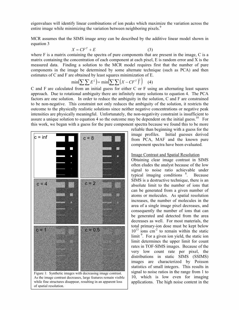
c = 4

c = inf c = 8

c = 2

c = 1 c = 0.5

Figure 1: Synthetic images with decreasing image contrast.

As the image contrast decreases, large features remain visible

while fine structures disappear, resulting in an apparent loss

of spatial resolution.

images makes both the visual interpretation of the results and the application of many statistical

image processing methods like histograms and thresholding problematic.

For the purposes of this paper, contrast between two regions in an image, c1,2 , is defined by

equation 1

2,1

21

2,1σ

IIc

−= (5)

where I1 is the average intensity in region 1, I2 is the average intensity in region 2 and σ1,2 is the

pooled standard deviation of the intensity within the two regions. The relevant value for c1,2 is the

threshold at which the boundaries between the two regions can be clearly seen with the human eye.

Precise values of the threshold are subjective and will vary from viewer to viewer. In figure 1, it

can be seen that the threshold is a function of the size (in pixels) of structures within the region. For

large features, this threshold is surprisingly low, <1. For 4x4 pixel features, the threshold occurs at

c ≈ 2. For 2x2 pixel features, the threshold occurs at c ≈ 4. Note that the image contrast can be

increased by either increasing the average difference between the two regions or decrease the

standard deviation within the regions. As a result, any form of de-noising will tend to increase the

image contrast.

For low count/pixel SIMS images, spatial resolution and image contrast are inherently linked.

Spatial resolution will ultimately be limited by the contrast threshold. In this paper, we will not

directly explore resolution but will

instead rely on image contrast as an

indicator of this feature.

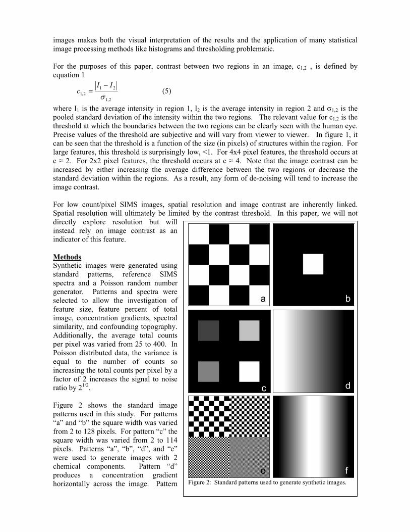
Methods Synthetic images were generated using

standard patterns, reference SIMS

spectra and a Poisson random number

generator. Patterns and spectra were

selected to allow the investigation of

feature size, feature percent of total

image, concentration gradients, spectral

similarity, and confounding topography.

Additionally, the average total counts

per pixel was varied from 25 to 400. In

Poisson distributed data, the variance is

equal to the number of counts so

increasing the total counts per pixel by a

factor of 2 increases the signal to noise

ratio by 21/2.

Figure 2 shows the standard image

patterns used in this study. For patterns

“a” and “b” the square width was varied

from 2 to 128 pixels. For pattern “c” the

square width was varied from 2 to 114

pixels. Patterns “a”, “b”, “d”, and “e”

were used to generate images with 2

chemical components. Pattern “d”

produces a concentration gradient

horizontally across the image. Pattern

a b

c d

e fFigure 2: Standard patterns used to generate synthetic images.

a b

c d

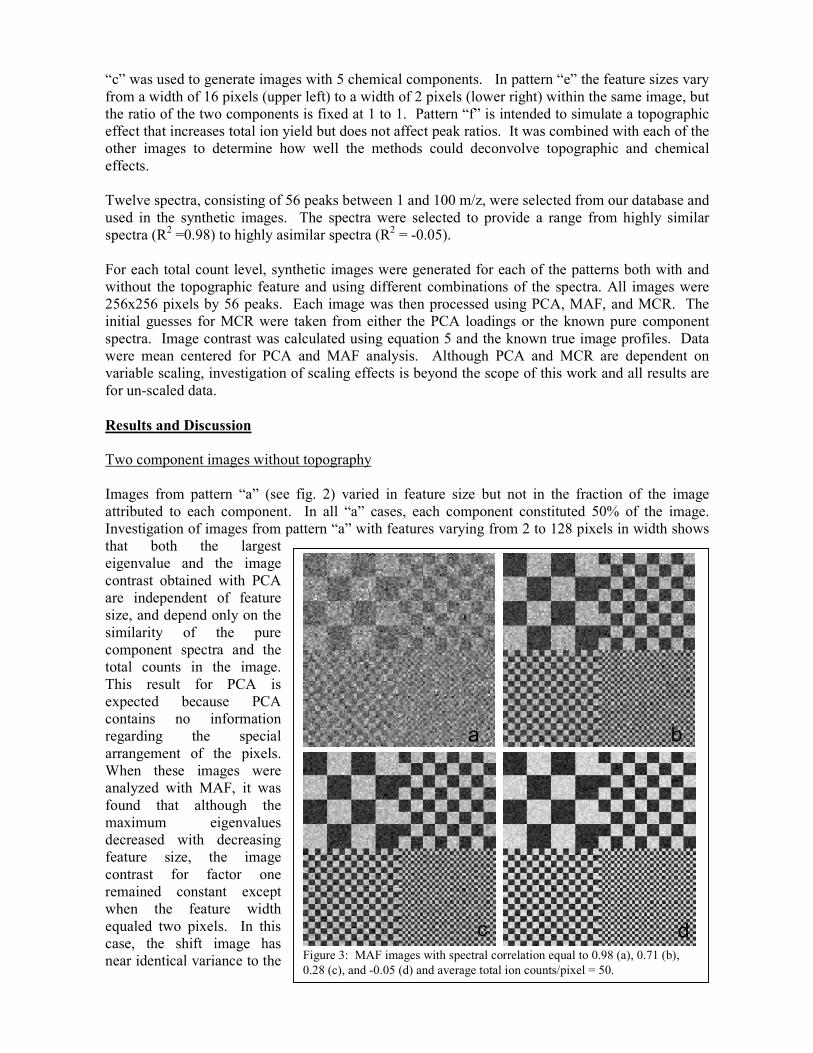
Figure 3: MAF images with spectral correlation equal to 0.98 (a), 0.71 (b),

0.28 (c), and -0.05 (d) and average total ion counts/pixel = 50.

“c” was used to generate images with 5 chemical components. In pattern “e” the feature sizes vary

from a width of 16 pixels (upper left) to a width of 2 pixels (lower right) within the same image, but

the ratio of the two components is fixed at 1 to 1. Pattern “f” is intended to simulate a topographic

effect that increases total ion yield but does not affect peak ratios. It was combined with each of the

other images to determine how well the methods could deconvolve topographic and chemical

effects.

Twelve spectra, consisting of 56 peaks between 1 and 100 m/z, were selected from our database and

used in the synthetic images. The spectra were selected to provide a range from highly similar

spectra (R2 =0.98) to highly asimilar spectra (R

2 = -0.05).

For each total count level, synthetic images were generated for each of the patterns both with and

without the topographic feature and using different combinations of the spectra. All images were

256x256 pixels by 56 peaks. Each image was then processed using PCA, MAF, and MCR. The

initial guesses for MCR were taken from either the PCA loadings or the known pure component

spectra. Image contrast was calculated using equation 5 and the known true image profiles. Data

were mean centered for PCA and MAF analysis. Although PCA and MCR are dependent on

variable scaling, investigation of scaling effects is beyond the scope of this work and all results are

for un-scaled data.

Results and Discussion

Two component images without topography

Images from pattern “a” (see fig. 2) varied in feature size but not in the fraction of the image

attributed to each component. In all “a” cases, each component constituted 50% of the image.

Investigation of images from pattern “a” with features varying from 2 to 128 pixels in width shows

that both the largest

eigenvalue and the image

contrast obtained with PCA

are independent of feature

size, and depend only on the

similarity of the pure

component spectra and the

total counts in the image.

This result for PCA is

expected because PCA

contains no information

regarding the special

arrangement of the pixels.

When these images were

analyzed with MAF, it was

found that although the

maximum eigenvalues

decreased with decreasing

feature size, the image

contrast for factor one

remained constant except

when the feature width

equaled two pixels. In this

case, the shift image has

near identical variance to the

-0.2 0 0.2 0.4 0.6 0.8 1 1.20

2

4

6

8

10

12

14

spectral correlation

image contrast

MAFPCAMCRBest Peak

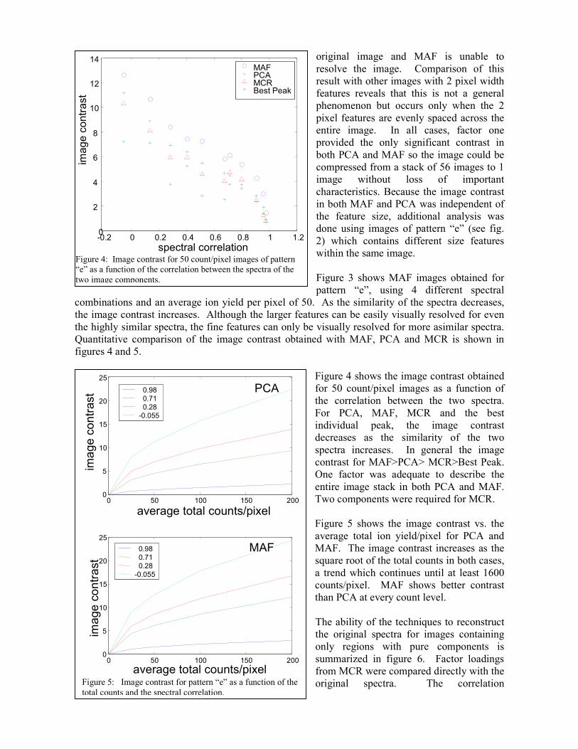
Figure 4: Image contrast for 50 count/pixel images of pattern

“e” as a function of the correlation between the spectra of the

two image components.

0 50 100 150 2000

5

10

15

20

25

average total counts/pixel

image contrast

0 50 100 150 2000

5

10

15

20

25

average total counts/pixel

image contrast

0.98

0.71

0.28

-0.055

0.98

0.71

0.28

-0.055

PCA

MAF

Figure 5: Image contrast for pattern “e” as a function of the

total counts and the spectral correlation.

original image and MAF is unable to

resolve the image. Comparison of this

result with other images with 2 pixel width

features reveals that this is not a general

phenomenon but occurs only when the 2

pixel features are evenly spaced across the

entire image. In all cases, factor one

provided the only significant contrast in

both PCA and MAF so the image could be

compressed from a stack of 56 images to 1

image without loss of important

characteristics. Because the image contrast

in both MAF and PCA was independent of

the feature size, additional analysis was

done using images of pattern “e” (see fig.

2) which contains different size features

within the same image.

Figure 3 shows MAF images obtained for

pattern “e”, using 4 different spectral

combinations and an average ion yield per pixel of 50. As the similarity of the spectra decreases,

the image contrast increases. Although the larger features can be easily visually resolved for even

the highly similar spectra, the fine features can only be visually resolved for more asimilar spectra.

Quantitative comparison of the image contrast obtained with MAF, PCA and MCR is shown in

figures 4 and 5.

Figure 4 shows the image contrast obtained

for 50 count/pixel images as a function of

the correlation between the two spectra.

For PCA, MAF, MCR and the best

individual peak, the image contrast

decreases as the similarity of the two

spectra increases. In general the image

contrast for MAF>PCA> MCR>Best Peak.

One factor was adequate to describe the

entire image stack in both PCA and MAF.

Two components were required for MCR.

Figure 5 shows the image contrast vs. the

average total ion yield/pixel for PCA and

MAF. The image contrast increases as the

square root of the total counts in both cases,

a trend which continues until at least 1600

counts/pixel. MAF shows better contrast

than PCA at every count level.

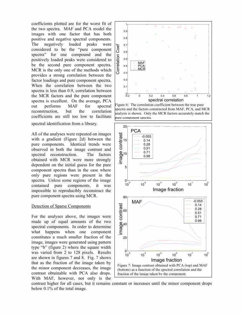
The ability of the techniques to reconstruct

the original spectra for images containing

only regions with pure components is

summarized in figure 6. Factor loadings

from MCR were compared directly with the

original spectra. The correlation

-0.2 0 0.2 0.4 0.6 0.8 1 1.20

0.1

0.2

0.3

0.4

0.5

0.6

0.7

0.8

0.9

1

spectral correlation

Correlation Coef

MAFPCAMCR

Figure 6: The correlation coefficient between the true pure

spectra and the factors constructed from MAF, PCA, and MCR

analysis is shown. Only the MCR factors accurately match the

pure component spectra.

10-5

10-4

10-3

10-2

10-1

100

0

20

40

60

80

Image fraction

image contrast -0.055

0.14

0.28

0.51

0.71

0.98

10-5

10-4

10-3

10-2

10-1

100

0

5

10

15

20

Image fraction

image contrast

-0.055

0.14

0.28

0.51

0.71

0.98

PCA

MAF

Figure 7: Image contrast obtained with PCA (top) and MAF

(bottom) as a function of the spectral correlation and the

fraction of the image taken by the component.

coefficients plotted are for the worst fit of

the two spectra. MAF and PCA model the

images with one factor that has both

positive and negative spectral components.

The negatively loaded peaks were

considered to be the “pure component

spectra” for one compound and the

positively loaded peaks were considered to

be the second pure component spectra.

MCR is the only one of the methods which

provides a strong correlation between the

factor loadings and pure component spectra.

When the correlation between the two

spectra is less than 0.9, correlation between

the MCR factors and the pure component

spectra is excellent. On the average, PCA

out performs MAF for spectral

reconstruction, but the correlation

coefficients are still too low to facilitate

spectral identification from a library.

All of the analyses were repeated on images

with a gradient (Figure 2d) between the

pure components. Identical trends were

observed in both the image contrast and

spectral reconstruction. The factors

obtained with MCR were more strongly

dependent on the initial guess for the pure

component spectra than in the case where

only pure regions were present in the

spectra. Unless some regions of the image

contained pure components, it was

impossible to reproducibly reconstruct the

pure component spectra using MCR.

Detection of Sparse Components

For the analyses above, the images were

made up of equal amounts of the two

spectral components. In order to determine

what happens when one component

constitutes a much smaller fraction of the

image, images were generated using pattern

type “b” (figure 2) where the square width

was varied from 2 to 128 pixels. Results

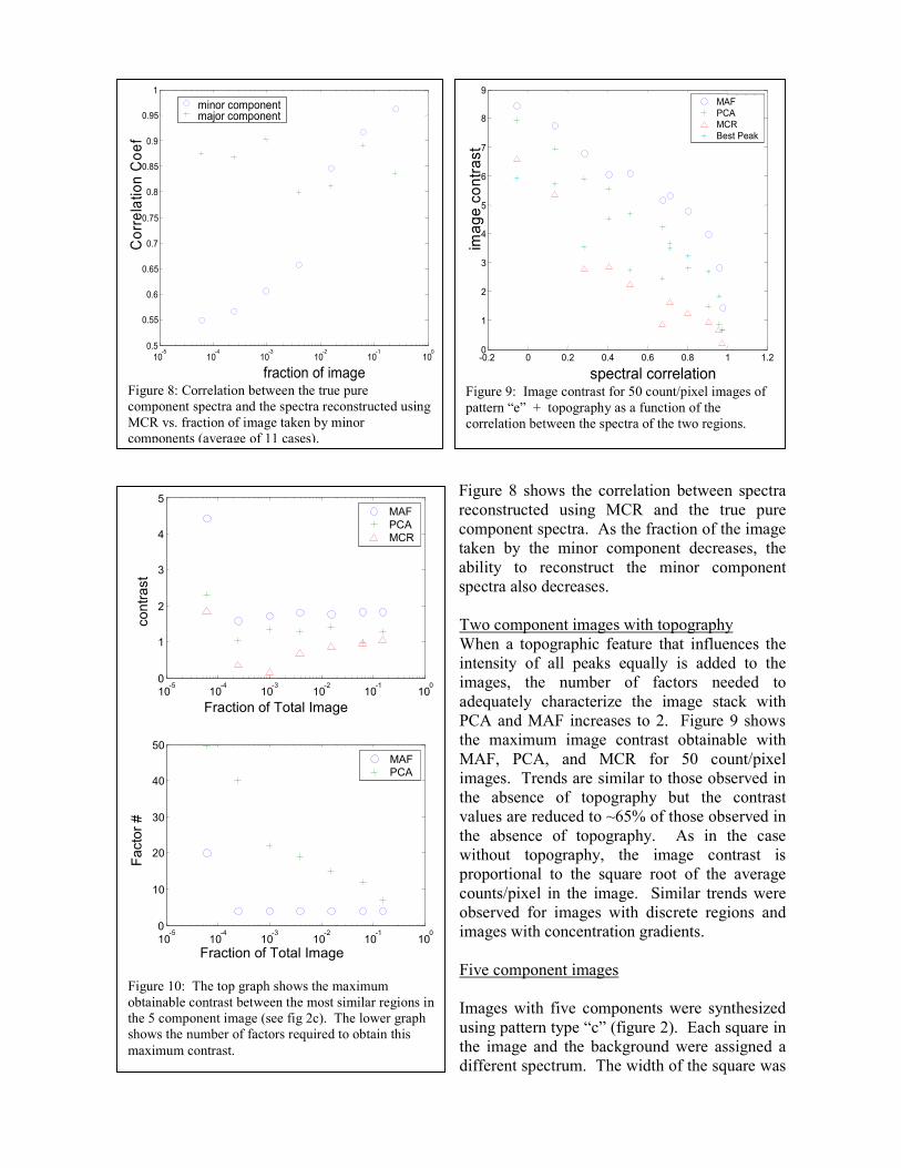
are shown in figures 7 and 8. Fig. 7 shows

that as the fraction of the image taken by

the minor component decreases, the image

contrast obtainable with PCA also drops.

With MAF, however, not only is the

contrast higher for all cases, but it remains constant or increases until the minor component drops

below 0.1% of the total image.

10-5

10-4

10-3

10-2

10-1

100

0.5

0.55

0.6

0.65

0.7

0.75

0.8

0.85

0.9

0.95

1

fraction of image

Correlation Coef

minor componentmajor component

Figure 8: Correlation between the true pure

component spectra and the spectra reconstructed using

MCR vs. fraction of image taken by minor

components (average of 11 cases).

-0.2 0 0.2 0.4 0.6 0.8 1 1.20

1

2

3

4

5

6

7

8

9

spectral correlation

image contrast

MAF

PCA

MCR

Best Peak

Figure 9: Image contrast for 50 count/pixel images of

pattern “e” + topography as a function of the

correlation between the spectra of the two regions.

10-5

10-4

10-3

10-2

10-1

100

0

1

2

3

4

5

Fraction of Total Image

contrast

MAF

PCA

MCR

10-5

10-4

10-3

10-2

10-1

100

0

10

20

30

40

50

Fraction of Total Image

Factor #

MAF

PCA

Figure 10: The top graph shows the maximum

obtainable contrast between the most similar regions in

the 5 component image (see fig 2c). The lower graph

shows the number of factors required to obtain this

maximum contrast.

Figure 8 shows the correlation between spectra

reconstructed using MCR and the true pure

component spectra. As the fraction of the image

taken by the minor component decreases, the

ability to reconstruct the minor component

spectra also decreases.

Two component images with topography

When a topographic feature that influences the

intensity of all peaks equally is added to the

images, the number of factors needed to

adequately characterize the image stack with

PCA and MAF increases to 2. Figure 9 shows

the maximum image contrast obtainable with

MAF, PCA, and MCR for 50 count/pixel

images. Trends are similar to those observed in

the absence of topography but the contrast

values are reduced to ~65% of those observed in

the absence of topography. As in the case

without topography, the image contrast is

proportional to the square root of the average

counts/pixel in the image. Similar trends were

observed for images with discrete regions and

images with concentration gradients.

Five component images

Images with five components were synthesized

using pattern type “c” (figure 2). Each square in

the image and the background were assigned a

different spectrum. The width of the square was

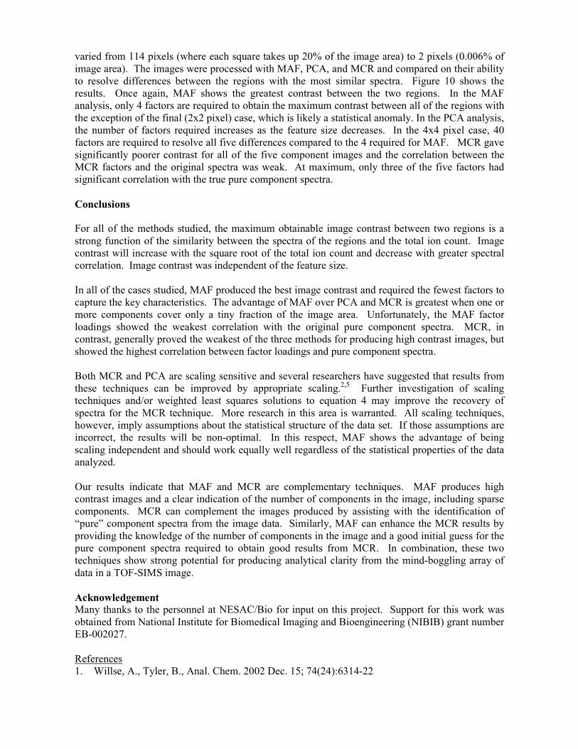
varied from 114 pixels (where each square takes up 20% of the image area) to 2 pixels (0.006% of

image area). The images were processed with MAF, PCA, and MCR and compared on their ability

to resolve differences between the regions with the most similar spectra. Figure 10 shows the

results. Once again, MAF shows the greatest contrast between the two regions. In the MAF

analysis, only 4 factors are required to obtain the maximum contrast between all of the regions with

the exception of the final (2x2 pixel) case, which is likely a statistical anomaly. In the PCA analysis,

the number of factors required increases as the feature size decreases. In the 4x4 pixel case, 40

factors are required to resolve all five differences compared to the 4 required for MAF. MCR gave

significantly poorer contrast for all of the five component images and the correlation between the

MCR factors and the original spectra was weak. At maximum, only three of the five factors had

significant correlation with the true pure component spectra.

Conclusions

For all of the methods studied, the maximum obtainable image contrast between two regions is a

strong function of the similarity between the spectra of the regions and the total ion count. Image

contrast will increase with the square root of the total ion count and decrease with greater spectral

correlation. Image contrast was independent of the feature size.

In all of the cases studied, MAF produced the best image contrast and required the fewest factors to

capture the key characteristics. The advantage of MAF over PCA and MCR is greatest when one or

more components cover only a tiny fraction of the image area. Unfortunately, the MAF factor

loadings showed the weakest correlation with the original pure component spectra. MCR, in

contrast, generally proved the weakest of the three methods for producing high contrast images, but

showed the highest correlation between factor loadings and pure component spectra.

Both MCR and PCA are scaling sensitive and several researchers have suggested that results from

these techniques can be improved by appropriate scaling.2,5 Further investigation of scaling

techniques and/or weighted least squares solutions to equation 4 may improve the recovery of

spectra for the MCR technique. More research in this area is warranted. All scaling techniques,

however, imply assumptions about the statistical structure of the data set. If those assumptions are

incorrect, the results will be non-optimal. In this respect, MAF shows the advantage of being

scaling independent and should work equally well regardless of the statistical properties of the data

analyzed.

Our results indicate that MAF and MCR are complementary techniques. MAF produces high

contrast images and a clear indication of the number of components in the image, including sparse

components. MCR can complement the images produced by assisting with the identification of

“pure” component spectra from the image data. Similarly, MAF can enhance the MCR results by

providing the knowledge of the number of components in the image and a good initial guess for the

pure component spectra required to obtain good results from MCR. In combination, these two

techniques show strong potential for producing analytical clarity from the mind-boggling array of

data in a TOF-SIMS image.

Acknowledgement Many thanks to the personnel at NESAC/Bio for input on this project. Support for this work was

obtained from National Institute for Biomedical Imaging and Bioengineering (NIBIB) grant number

EB-002027.

References

1. Willse, A., Tyler, B., Anal. Chem. 2002 Dec. 15; 74(24):6314-22

2. Keenan, M.R., Kotula, P.G., Surface and Interface Analysis, Volume 36, Issue 3 , Pages 203 -

212

3. Nygren, H. and Malmberg, P., Journal of Microscopy, Vol. 215, Pt 2, (2004), pp. 156-161

4. Biesinger, M. C, Paepegaey, P.-Y., McIntyre, N. S., Harbottle, R. R., Petersen, N. O.,

Anal. Chem. , 2002; 74(22); 5711-5716

5. Smentkowski, V. S.; Keenan, M. R.; Ohlhausen, J. A.; Kotula, P. G.;

Anal. Chem.; (Technical Note); 2005; 77(5); 1530-1536

6. Wolkenstein, M., Hutter, H.; Mittermayr, C.; Schiesser, W.; Grasserbauer, M., Anal. Chem.

1997, 69, 777-782

7. McLachIan, G. J., Discriminant Analysis and Statistical Pattern Recognition; Wiley: New

York, 1992; Chapter 13

8. McCuliagh, P., Nelder, J. A., Generalized Linear Models, 2nd ed.; Chapman & Hall: London,

1989; Chapter 6

9. R. Larsen, J. of Chemometrics, 16(8-10), 427-435 (2002)

10. Haaland, D. M., Timlin, J. A., Sinclair, M. B., Van Benthem, M. H., Martinez, M. J., Aragon,

A. D. & Werner-Washburne, M. (2003) in Spectral Imaging: Instrumentation, Applications,

and Analysis, (Publisher: International Society for Optical Engineering, San Jose, CA), Vol.

4959, paper 06