multivariate notes r1 - College of Education | U of I

Version: June 19, 2007

Notes for Applied MultivariateAnalysis with MATLAB

These notes were written for use within Quantitative Psychology

courses at the University of Illinois, Champaign. The expectation is

that for Psychology 406/7 (Statistical Methods I and II), the mate-

rial up through Section 0.1.12 be available to a student. For Mul-

tivariate Analysis (Psychology 594) and Covariance Structure and

Factor Models (Psychology 588), the remainder of the notes are rel-

evant, with particular emphasis on Singular Value Decomposition

(SVD) and Eigenvector/Eigenvalue Decomposition (Spectral Decom-

position).

1

Contents

0.1 Necessary Matrix Algebra Tools . . . . . . . . . . . . 5

0.1.1 Preliminaries . . . . . . . . . . . . . . . . . . 5

0.1.2 The Data Matrix . . . . . . . . . . . . . . . . 12

0.1.3 Inner Products . . . . . . . . . . . . . . . . . 13

0.1.4 Determinants . . . . . . . . . . . . . . . . . . 17

0.1.5 Linear Independence/Dependence of Vectors . 19

0.1.6 Matrix Inverses . . . . . . . . . . . . . . . . . 20

0.1.7 Matrices as Transformations . . . . . . . . . . 23

0.1.8 Matrix and Vector Orthogonality . . . . . . . 25

0.1.9 Matrix Rank . . . . . . . . . . . . . . . . . . 25

0.1.10 Using Matrices to Solve Equations . . . . . . 29

0.1.11 Quadratic Forms . . . . . . . . . . . . . . . . 30

0.1.12 Multiple Regression . . . . . . . . . . . . . . 31

0.2 Eigenvectors and Eigenvalues . . . . . . . . . . . . . 33

0.3 The Singular Value Decomposition of a Matrix . . . . 41

0.4 Common Multivariate Methods in Matrix Terms . . . 42

0.4.1 Principal Components . . . . . . . . . . . . . 42

0.4.2 Discriminant Analysis . . . . . . . . . . . . . 43

0.4.3 Canonical Correlation . . . . . . . . . . . . . 44

0.4.4 Algebraic Restrictions on Correlations . . . . . 46

0.4.5 The Biplot . . . . . . . . . . . . . . . . . . . 47

2

0.4.6 The Procrustes Problem . . . . . . . . . . . . 49

0.4.7 Matrix Rank Reduction . . . . . . . . . . . . 50

0.4.8 Torgerson Metric Multidimensional Scaling . . 50

0.4.9 A Guttman Multidimensional Scaling Result . 52

0.4.10 A Few General MATLAB Routines to Know

About . . . . . . . . . . . . . . . . . . . . . . 53

3

List of Figures

1 Two vectors plotted in two-dimensional space . . . . 15

2 Illustration of projecting one vector onto another . . . 16

4

0.1 Necessary Matrix Algebra Tools

The strategies of multivariate analysis tend to be confusing unless

specified compactly in matrix terms. Therefore, we will spend some

significant amount of time on these topics because, in fact, most of

multivariate analysis falls out directly once we have these tools under

control. Remember the old Saturday Night Live skit with Hans and

Franz, “listen to me now, and believe me later”. I have a goal in mind

of where I would like you all to be — at the point of understanding

and being able to work with what is called the Singular Value De-

composition (SVD) of a matrix, and to understand the matrix topics

that lead up to the SVD. Very much like teaching how to use some

word-processing program, where we need to learn all the various com-

mands and what they do, an introduction to the matrix tools can

seem a little disjointed. But just like word-processing comes together

more meaningfully when required to do your own manuscripts from

beginning to end, once we proceed into the techniques of multivariate

analysis per se, the wisdom of this preliminary matrix excursion will

be apparent.

0.1.1 Preliminaries

A matrix is merely an array of numbers; for example,⎛⎜⎜⎜⎜⎜⎝

4 −1 3 1

4 6 0 2

7 2 1 4

⎞⎟⎟⎟⎟⎟⎠

is a matrix. In general, we denote a matrix by an uppercase (capi-

tal) boldface letter such as A (or using a proofreader representation

5

on the blackboard, a capital letter with a wavy line underneath to

indicate boldface):

A =

⎛⎜⎜⎜⎜⎜⎜⎜⎜⎝

a11 a12 a13 · · · a1V

a21 a22 a23 · · · a2V... ... ... . . . ...

aU1 aU2 aU3 · · · aUV

⎞⎟⎟⎟⎟⎟⎟⎟⎟⎠

This matrix has U rows and V columns and is said to have order

U × V . An arbitrary element auv refers to the element in the uth

row and vth column, with the row index always preceding the column

index (and therefore, we might use the notation of A = {auv}U×V

to indicate the matrix A as well as its order).

A 1× 1 matrix such as (4)1×1 is just an ordinary number, called a

scalar. So without loss of any generality, numbers are just matrices.

A vector is a matrix with a single row or column; we denote a column

vector by a lowercase boldface letter, e.g., x, y, z, and so on. The

vector

x =

⎛⎜⎜⎜⎜⎜⎝

x1...

xU

⎞⎟⎟⎟⎟⎟⎠

U×1

is of order U×1; the column indices are typically omitted since there

is only one. A row vector is written as

x′ = (x1, . . . , xU)1×U

with the prime indicating the transpose of x, i.e., the interchange of

row(s) and column(s). This transpose operation can be applied to

any matrix; for example,

6

A =

⎛⎜⎜⎜⎜⎜⎝

1 −1

3 7

4 1

⎞⎟⎟⎟⎟⎟⎠

3×2

A′ =

⎛⎜⎝ 1 3 4

−1 7 1

⎞⎟⎠

2×3

If a matrix is square, defined by having the same number of rows

as columns, say U , and if the matrix and its transpose are equal, the

matrix is said to be symmetric. Thus, in A = {auv}U×U , auv = avu

for all u and v. As an example,

A = A′ =

⎛⎜⎜⎜⎜⎜⎝

1 4 3

4 7 −1

3 −1 3

⎞⎟⎟⎟⎟⎟⎠

For a square matrix AU×U , the elements auu, 1 ≤ u ≤ U , lie along

the main or principal diagonal. The sum of main diagonal entries

of a square matrix is called the trace ; thus,

trace(AU×U ) ≡ tr(A) = a11 + · · · + aUU

A number of special matrices appear periodically in the notes to

follow. A U×V matrix of all zeros is called a null matrix, and might

be denoted by

∅ =

⎛⎜⎜⎜⎜⎜⎝

0 · · · 0... . . . ...

0 · · · 0

⎞⎟⎟⎟⎟⎟⎠

7

Similarly, we might at times need an U × V matrix of all ones, say

E:

E =

⎛⎜⎜⎜⎜⎜⎝

1 · · · 1... . . . ...

1 · · · 1

⎞⎟⎟⎟⎟⎟⎠

A diagonal matrix is square with zeros in all the off main-diagonal

positions:

DU×U =

⎛⎜⎜⎜⎜⎜⎝

a1 · · · 0... . . . ...

0 · · · aU

⎞⎟⎟⎟⎟⎟⎠

U×U

Here, we again indicate the main diagonal entries with just one index

as a1, a2, . . . , aU . If all of the main diagonal entries in a diagonal

matrix are 1s, we have the identity matrix denoted by I:

I =

⎛⎜⎜⎜⎜⎜⎜⎜⎜⎝

1 0 · · · 0

0 1 · · · 0... ... . . . ...

0 0 · · · 1

⎞⎟⎟⎟⎟⎟⎟⎟⎟⎠

To introduce some useful operations on matrices, suppose we have

two matrices A and B of the same U × V order:

A =

⎛⎜⎜⎜⎜⎜⎝

a11 · · · a1V... . . . ...

aU1 · · · aUV

⎞⎟⎟⎟⎟⎟⎠

U×V

B =

⎛⎜⎜⎜⎜⎜⎝

b11 · · · b1V... . . . ...

bU1 · · · bUV

⎞⎟⎟⎟⎟⎟⎠

U×V

8

As a definition for equality of two matrices of the same order (and

for which it only makes sense to talk about equality), we have:

A = B if and only if auv = buv for all u and v.

Remember, the “if and only if” statement (sometimes abbreviated

as “iff”) implies two conditions:

if A = B, then auv = buv for all u and v;

if auv = buv for all u and v, then A = B.

Any definition by its very nature implies an “if and only if” state-

ment.

To add two matrices together, they first have to be of the same

order (referred to as conformal for addition); we then do the addition

component by component:

A + B =

⎛⎜⎜⎜⎜⎜⎝

a11 + b11 · · · a1V + b1V... . . . ...

aU1 + bU1 · · · aUV + bUV

⎞⎟⎟⎟⎟⎟⎠

U×V

To preform scalar multiplication of a matrix A by, say, a constant

c, we again do the multiplication component by component:

cA =

⎛⎜⎜⎜⎜⎜⎝

ca11 · · · ca1V... . . . ...

caU1 · · · caUV

⎞⎟⎟⎟⎟⎟⎠ = c

⎛⎜⎜⎜⎜⎜⎝

a11 · · · a1V... . . . ...

aU1 · · · aUV

⎞⎟⎟⎟⎟⎟⎠

Thus, if one wished to define the difference of two matrices, we could

proceed rather obviously as follows:

A − B ≡ A + (−1)B = {auv − buv}One of the more important matrix operations is multiplication

where two matrices are said to be conformal for multiplication if the

9

number of rows in one matches the number of columns in the second.

For example, suppose A is U×V and B is V ×W ; then, because the

number of columns in A matches the number of rows in B, we can

define AB as CU×W , where {cuw} = {∑Vk=1 aukbkw}. This process

might be referred to as row (of A) by column (of B) multiplication;

the following simple example should make this clear:

A3×2 =

⎛⎜⎜⎜⎜⎜⎝

1 4

3 1

−1 0

⎞⎟⎟⎟⎟⎟⎠ , B2×4 =

⎛⎜⎝ −1 2 0 1

1 0 1 4

⎞⎟⎠ ;

AB = C3×4 =⎛⎜⎜⎜⎜⎜⎝

1(−1) + 4(1) 1(2) + 4(0) 1(0) + 4(1) 1(1) + 4(4)

3(−1) + 1(1) 3(2) + 1(0) 3(0) + 1(1) 3(1) + 1(4)

−1(−1) + 0(1) −1(2) + 0(0) −1(0) + 0(1) −1(1) + 0(4)

⎞⎟⎟⎟⎟⎟⎠ =

⎛⎜⎜⎜⎜⎜⎝

3 2 4 17

−2 6 1 7

1 −2 0 −1

⎞⎟⎟⎟⎟⎟⎠

Some properties of matrix addition and multiplication follow, where

the matrices are assumed conformal for the operations given:

(A) matrix addition is commutative:

A + B = B + A

(B) matrix addition is associative:

A + (B + C) = (A + B) + C

10

(C) matrix multiplication is right and left distributive over matrix

addition:

A(B + C) = AB + AC

(A + B)C = AC + BC

(D) matrix multiplication is associative:

A(BC) = (AB)C

In general, AB �= BA even if both products are defined. Thus,

multiplication is not commutative as the following simple example

shows:

A2×2 =

⎛⎜⎝ 0 1

1 0

⎞⎟⎠ ; B2×2 =

⎛⎜⎝ 1 1

0 1

⎞⎟⎠ ; AB =

⎛⎜⎝ 0 1

1 1

⎞⎟⎠ ; BA =

⎛⎜⎝ 1 1

1 0

⎞⎟⎠

In the product AB, we say that B is premultiplied by A and A

is postmultiplied by B. Thus, if we pre- or postmultiply a matrix

by the identity, the same matrix is retrieved:

IU×UAU×V = AU×V ; AU×V IV ×V = AU×V

If we premultiply A by a diagonal matrix D, then each row of A is

multiplied by a particular diagonal entry in D:

DU×UAU×V =

⎛⎜⎜⎜⎜⎜⎝

d1a11 · · · d1a1V... . . . ...

dUar1 · · · dUaUV

⎞⎟⎟⎟⎟⎟⎠

If A is post-multiplied by a diagonal matrix D, then each column of

A is multiplied by a particular diagonal entry in D:

11

AU×V DV ×V =

⎛⎜⎜⎜⎜⎜⎝

d1a11 · · · dV a1V... . . . ...

d1aU1 · · · dV aUV

⎞⎟⎟⎟⎟⎟⎠

Finally, we end this section with a few useful results on the transpose

operation and matrix multiplication and addition:

(AB)′ = B′A′; (ABC)′ = C′B′A′; . . .

(A′)′ = A; (A + B)′ = A′ + B′

0.1.2 The Data Matrix

A very common type of matrix encountered in multivariate analysis

is what is referred to as a data matrix containing, say, observations

for N subjects on P variables. We will typically denote this matrix

by XN×P = {xij}, with a generic element of xij referring to the

observation for subject or row i on variable or column j (1 ≤ i ≤ N

and 1 ≤ j ≤ P ):

XN×P =

⎛⎜⎜⎜⎜⎜⎜⎜⎜⎝

x11 x12 · · · x1P

x21 x22 · · · x2P... ... . . . ...

xN1 xN2 · · · xNP

⎞⎟⎟⎟⎟⎟⎟⎟⎟⎠

All right-thinking people always list subjects as rows and variables

as columns, conforming also to the now-common convention for com-

puter spreadsheets.

Any matrix in general, including a data matrix, can be viewed

either as a collection of its row vectors or of its column vectors,

12

and these interpretations can be generally useful. For a data matrix

XN×P , let x′i = (xi1, . . . , xiP )1×P denote the row vector for subject

i, 1 ≤ i ≤ N , and let vj denote the N ×1 column vector for variable

j:

vj =

⎛⎜⎜⎜⎜⎜⎝

x1j...

xNj

⎞⎟⎟⎟⎟⎟⎠

N×1

Thus, each subject could be viewed as providing a vector of coordi-

nates (1 × P ) in P -dimensional “variable space”, where the P axes

correspond to the P variables; or each variable could be viewed as

providing a vector of coordinates (N × 1) in “subject space”, where

the N axes correspond to the N subjects:

XN×P =

⎛⎜⎜⎜⎜⎜⎜⎜⎜⎝

x′1

x′2...

x′N

⎞⎟⎟⎟⎟⎟⎟⎟⎟⎠

=(v1 v2 · · · vP

)

0.1.3 Inner Products

The inner product (also called the dot or scalar product) of two

vectors , xU×1 and yU×1, is defined as

x′y = (x1, . . . , xU)

⎛⎜⎜⎜⎜⎜⎝

y1...

yU

⎞⎟⎟⎟⎟⎟⎠ =

U∑u=1

xuyu

Thus, the inner product of a vector with itself is merely the sum of

squares of the entries in the vector: x′x =∑U

u=1 x2u. Also, because

13

an inner product is a scalar and must equal it own transpose (i.e.,

x′y = (x′y)′ = y′x), we have the end result that

x′y = y′x

If there is an inner product, there should also be an outer product

defined as the U × U matrices given by xy′ or as yx′. As indicated

by the display equations below, xy′ is the transpose of yx′:

xy′ =

⎛⎜⎜⎜⎜⎜⎝

x1...

xU

⎞⎟⎟⎟⎟⎟⎠ (y1, . . . , yN) =

⎛⎜⎜⎜⎜⎜⎝

x1y1 · · · x1yU... . . . ...

xUy1 · · · xUyU

⎞⎟⎟⎟⎟⎟⎠

yx′ =

⎛⎜⎜⎜⎜⎜⎝

y1...

yU

⎞⎟⎟⎟⎟⎟⎠ (x1, . . . , xU) =

⎛⎜⎜⎜⎜⎜⎝

y1x1 · · · y1xU... . . . ...

yUx1 · · · yUxU

⎞⎟⎟⎟⎟⎟⎠

A vector can be viewed as a geometrical vector in U dimensional

space. Thus, the two 2 × 1 vectors

x =

⎛⎜⎝ 3

4

⎞⎟⎠ ; y =

⎛⎜⎝ 4

1

⎞⎟⎠

can be represented in the two-dimensional Figure 1 below, with the

entries in the vectors defining the coordinates of the endpoints of the

arrows.

The Euclidean distance between two vectors, x and y, is given

as: √√√√√ U∑u=1

(xu − yu)2 =√(x − y)′(x − y)

and the length of any vector is the Euclidean distance between the

vector and the origin. Thus, in Figure 1, the distance between x and

y is√

10 with respective lengths of 5 and√

17.

14

�

�

�������������

������

�������

(3,4)

(4,1)

(0,0)

θ

.

...............................

...............................

...............................

..............................

............................

.............................

1 2 3 4

1

2

3

4

Figure 1: Two vectors plotted in two-dimensional space

The cosine of the angle between the two vectors x and y if defined

by:

cos(θ) =x′y

(x′x)1/2(y′y)1/2

Thus, in the figure we have

cos(θ) =

(3 4

) ⎛⎜⎝ 4

1

⎞⎟⎠

5√

17=

16

5√

17= .776

The cosine value of .776 corresponds to an angle of 39.1 degrees or

.68 radians; these later values can be found with the inverse (or arc)

cosine function (on, say, a hand calculator, or using MATLAB as we

suggest in the next section).

When the means of the entries in x and y are zero (i.e., deviations

from means have been taken), then cos(θ) is the correlation between

15

�������������

���

c2b2

a2........................

.......................

........................

.......................

.......................

......................

x

y

dy

θ

Figure 2: Illustration of projecting one vector onto another

the entries in the two vectors. Vectors at right angles have cos(θ) = 0,

or alternatively, the correlation is zero.

Figure 2 shows two generic vectors, x and y, where without loss

of any real generality, y is drawn horizontally in the plane and x

is projected at a right angle onto the vector y resulting in a point

defined as a multiple d of the vector y. The formula for d that

we demonstrate below is based on the Pythagorean theorem that

c2 = b2 + a2:

c2 = b2 + a2 ⇒ x′x = (x − dy)′(x − dy) + d2y′y ⇒

x′x = x′x − dx′y − dy′x + d2y′y + d2y′y ⇒

0 = −2dx′y + 2d2y′y ⇒16

d =x′yy′y

The diagram in Figure 2 is somewhat constricted in the sense that the

angle between the vectors shown is less than 90 degrees; this allows

the constant d to be positive. Other angles might lead to negative d

when defining the projection of x onto y, and would merely indicate

the need to consider the vector y oriented in the opposite (negative)

direction. Similarly, the vector y is drawn with a larger length than

x which gives a value for d that is less than 1.0; otherwise, d would

be greater than 1.0 indicating a need to stretch y to represent the

point of projection onto it.

There are other formulas possible based on this geometric infor-

mation: the length of the projection is merely d times the length of

y; and cos(θ) can be given as the length of dy divided by the length

of x, which is d√

y′y/√

x′x = x′y/(√

x′x√

y′y).

0.1.4 Determinants

To each square matrix, AU×U , there is an associated scalar called the

determinant of A that is denoted by |A| or det(A). Determinants

up to a 3 × 3 can be given by formula:

det((

a)1×1

) = a; det(

⎛⎜⎝ a b

c d

⎞⎟⎠

2×2

) = ad − bc;

det(

⎛⎜⎜⎜⎜⎜⎝

a b c

d e f

g h i

⎞⎟⎟⎟⎟⎟⎠

3×3

) = aei + dhc + gfb − (ceg + fha + idb)

17

Beyond a 3×3 we can use a recursive process illustrated below. This

requires the introduction of a few additional matrix terms that we

now give: for a square matrix AU×U , define Auv to be the (n −1) × (n − 1) submatrix of A constructed by deleting the uth row

and vth column of A. We call det(Auv) the minor of the entry auv;

the signed minor of (−1)u+v det(Auv) is called the cofactor of auv.

The recursive algorithm would chose some row or column (rather

arbitrarily), and find the cofactors for the entries in it; the cofactors

would then be weighted by the relevant entries and summed.

As an example, consider the 4 × 4 matrix⎛⎜⎜⎜⎜⎜⎜⎜⎜⎝

1 −1 3 1

−1 1 0 −1

3 2 1 2

1 2 4 3

⎞⎟⎟⎟⎟⎟⎟⎟⎟⎠

and choose the second row. The expression below involves the weighted

cofactors for 3×3 submatrices that can be obtained by formulas. Be-

yond a 4 × 4 there will be nesting of the processes:

(−1)((−1)2+1) det(

⎛⎜⎜⎜⎜⎜⎝

−1 3 1

2 1 2

2 4 3

⎞⎟⎟⎟⎟⎟⎠) + (1)((−1)2+2) det(

⎛⎜⎜⎜⎜⎜⎝

1 3 1

3 1 2

1 4 3

⎞⎟⎟⎟⎟⎟⎠)+

(0)((−1)2+3) det(

⎛⎜⎜⎜⎜⎜⎝

1 −1 1

3 2 2

1 2 3

⎞⎟⎟⎟⎟⎟⎠) + (−1)((−1)2+4) det(

⎛⎜⎜⎜⎜⎜⎝

1 −1 3

3 2 1

1 2 4

⎞⎟⎟⎟⎟⎟⎠) =

5 + (−15) + 0 + (−29) = −39

Another strategy to find the determinant of a matrix is to reduce it

a form in which we might note the determinant more or less by simple

18

inspection. The reductions could be carried out by operations that

have a known effect on the determinant; the form which we might

seek is a matrix that is either upper-triangular (all entries below the

main diagonal are all zero), lower-triangular (all entries above the

main diagonal are all zero), or diagonal. In these latter cases, the

determinant is merely the product of the diagonal elements. Once

found, we can note how the determinant might have been changed

by the reduction process and carry out the reverse changes to find

the desired determinant.

The properties of determinants that we could rely on in the above

iterative process are as follows:

(A) if one row of A is multiplied by a constant c, the new determinant

is c det(A); the same is true for multiplying a column by c;

(B) if two rows or two columns of a matrix are interchanged, the sign

of the determinant is changed;

(C) if two rows or two columns of a matrix are equal, the determinant

is zero;

(D) the determinant is unchanged by adding a multiple of some row

to another row; the same is true for columns;

(E) a zero row or column implies a zero determinant;

(F) det(AB) = det(A) det(B)

0.1.5 Linear Independence/Dependence of Vectors

Suppose I have a collection of K vectors each of size U×1, x1, . . . ,xK .

If no vector in the set can be written as a linear combination of the

remaining ones, the set of vectors is said to be linearly indepen-

dent ; otherwise, the vectors are linearly dependent. As an example,

19

consider the three vectors:

x1 =

⎛⎜⎜⎜⎜⎜⎝

1

4

0

⎞⎟⎟⎟⎟⎟⎠ ; x2 =

⎛⎜⎜⎜⎜⎜⎝

1

−1

1

⎞⎟⎟⎟⎟⎟⎠ ; x3 =

⎛⎜⎜⎜⎜⎜⎝

3

7

1

⎞⎟⎟⎟⎟⎟⎠

Because 2x1+x2 = x3, we have a linear dependence among the three

vectors; however, x1 and x2, or, x2 and x3, are linearly independent.

If the U vectors (each of size U × 1), x1,x2, . . . ,xU , are linearly

independent, then the collection defines a basis, i.e., any vector can

be written as a linear combination of x1,x2, . . . ,xU . For example,

using the standard basis, e1, e2, . . . , eU , where eu is a vector of all

zeros except for a single one in the uth position, any vector x′ =

(x1, . . . , xU) can be written as:⎛⎜⎜⎜⎜⎜⎜⎜⎜⎝

x1

x2...

xU

⎞⎟⎟⎟⎟⎟⎟⎟⎟⎠

= x1

⎛⎜⎜⎜⎜⎜⎜⎜⎜⎝

1

0...

0

⎞⎟⎟⎟⎟⎟⎟⎟⎟⎠

+ x2

⎛⎜⎜⎜⎜⎜⎜⎜⎜⎝

0

1...

0

⎞⎟⎟⎟⎟⎟⎟⎟⎟⎠

+ · · · + xU

⎛⎜⎜⎜⎜⎜⎜⎜⎜⎝

0

0...

1

⎞⎟⎟⎟⎟⎟⎟⎟⎟⎠

=

x1e1 + x2e2 + · · · + xUeU

Bases that consist of orthogonal vectors (where all inner products are

zero) are important later in what is known as principal components

analysis. The standard basis involves orthogonal vectors, and any

other basis may always be modified by what is called the Gram-

Schmidt orthogonalization process to produce a new basis that does

contain all orthogonal vectors.

0.1.6 Matrix Inverses

Suppose A and B are both square and of size U × U . If AB = I,

then B is said to be an inverse of A and is denoted by A−1(≡ B).

20

Also, if AA−1 = I, then A−1A = I holds automatically. If A−1

exists, the matrix A is said to be nonsingular ; if A−1 does not

exist, A is singular.

An example:⎛⎜⎝ 1 3

2 1

⎞⎟⎠

⎛⎜⎝ −1/5 3/5

2/5 −1/5

⎞⎟⎠ =

⎛⎜⎝ 1 0

0 1

⎞⎟⎠

⎛⎜⎝ −1/5 3/5

2/5 −1/5

⎞⎟⎠

⎛⎜⎝ 1 3

2 1

⎞⎟⎠ =

⎛⎜⎝ 1 0

0 1

⎞⎟⎠

Given a matrix A, the inverse A−1 can be found using the follow-

ing four steps:

(A) form a matrix of the same size as A containing the minors for

all entries of A;

(B) multiply the matrix of minors by (−1)u+v to produce the

matrix of cofactors;

(C) divide all entries in the cofactors matrix by det(A);

(D) the transpose of the matrix found in (C) gives A−1.

As a mnemonic device to remember these four steps, we have the

phrase “My Cat Does Tricks” for Minor, Cofactor, Determinant Di-

vision, Transpose” (I tried to work “my cat turns tricks” into the

appropriate phrase but failed with the second to the last “t”). Ob-

viously, an inverse exists for a matrix A if det(A) �= 0, allowing the

division in step (C) to take place.

An example: for

A =

⎛⎜⎜⎜⎜⎜⎝

1 3 2

0 1 1

0 2 1

⎞⎟⎟⎟⎟⎟⎠ ; det(A) = −1

21

Step (A), the matrix of minors:⎛⎜⎜⎜⎜⎜⎝

−1 0 0

−1 1 2

1 1 1

⎞⎟⎟⎟⎟⎟⎠

Step (B), the matrix of cofactors:⎛⎜⎜⎜⎜⎜⎝

−1 0 0

1 1 −2

1 −1 1

⎞⎟⎟⎟⎟⎟⎠

Step (C), determinant division:⎛⎜⎜⎜⎜⎜⎝

1 0 0

−1 −1 2

−1 1 −1

⎞⎟⎟⎟⎟⎟⎠

Step (D), matrix transpose:

A−1 =

⎛⎜⎜⎜⎜⎜⎝

1 −1 −1

0 −1 1

0 2 −1

⎞⎟⎟⎟⎟⎟⎠

We can easily verify that AA−1 = I:⎛⎜⎜⎜⎜⎜⎝

1 3 2

0 1 1

0 2 1

⎞⎟⎟⎟⎟⎟⎠

⎛⎜⎜⎜⎜⎜⎝

1 −1 −1

0 −1 1

0 2 −1

⎞⎟⎟⎟⎟⎟⎠ =

⎛⎜⎜⎜⎜⎜⎝

1 0 0

0 1 0

0 0 1

⎞⎟⎟⎟⎟⎟⎠

As a very simple instance of the mnemonic in the case of a 2 × 2

matrix with arbitrary entries:

A =

⎛⎜⎝ a b

c d

⎞⎟⎠

22

the inverse exists if det(A) = ad − bc �= 0:

A−1 =1

ad − bc

⎛⎜⎝ d −b

−c a

⎞⎟⎠

Several properties of inverses are given below that will prove useful

in our continuing presentation:

(A) if A is symmetric, then so is A−1;

(B) (A′)−1 = (A−1)′; or, the inverse of a transpose is the transpose

of the inverse;

(C) (AB)−1 = B−1A−1; (ABC)−1 = C−1B−1A−1; or, the in-

verse of a product is the product of inverses in the opposite order;

(D) (cA)−1 = (1c)A−1; or, the inverse of a scalar times a matrix

is the scalar inverse times the matrix inverse;

(E) the inverse of a diagonal matrix, is also diagonal with the

entries being the inverses of the entries from the original matrix (as-

suming none are zero):⎛⎜⎜⎜⎜⎜⎝

a1 · · · 0... . . . ...

0 · · · aU

⎞⎟⎟⎟⎟⎟⎠

−1

=

⎛⎜⎜⎜⎜⎜⎝

1a1

· · · 0... . . . ...

0 · · · 1aU

⎞⎟⎟⎟⎟⎟⎠

0.1.7 Matrices as Transformations

Any U × V matrix A can be seen as transforming a V × 1 vector

xV ×1 to another U × 1 vector yU×1:

yU×1 = AU×V xV ×1

or,

23

⎛⎜⎜⎜⎜⎜⎝

y1...

yU

⎞⎟⎟⎟⎟⎟⎠ =

⎛⎜⎜⎜⎜⎜⎝

a11 · · · a1V... . . . ...

aU1 · · · aUV

⎞⎟⎟⎟⎟⎟⎠

⎛⎜⎜⎜⎜⎜⎝

x1...

xV

⎞⎟⎟⎟⎟⎟⎠

where yu = au1x1 + au2x2 + · · · + auV xV . Alternatively, y can be

written as a linear combination of the columns of A with weights

given by x1, . . . , xV :⎛⎜⎜⎜⎜⎜⎝

y1...

yU

⎞⎟⎟⎟⎟⎟⎠ = x1

⎛⎜⎜⎜⎜⎜⎝

a11...

aU1

⎞⎟⎟⎟⎟⎟⎠ + x2

⎛⎜⎜⎜⎜⎜⎝

a12...

aU2

⎞⎟⎟⎟⎟⎟⎠ + · · · + xV

⎛⎜⎜⎜⎜⎜⎝

a1V...

aUV

⎞⎟⎟⎟⎟⎟⎠

To indicate one common usage for matrix transformation in a data

context, suppose we consider our data matrix X = {xij}N×P , where

xij represents an observation for subject i on variable j. We would

like to use matrix transformations to produce a standardized matrix

Z = {(xij − xj)/sj}N×P , where xj is the mean of the entries in

the jth column and sj is the corresponding standard deviation; thus,

the columns of Z all have mean zero and standard deviation one. A

matrix expression for this transformation could be written as follows:

ZN×P = (IN×N − (1

N)EN×N )XN×PDP×P

where I is the identity matrix, E contains all ones, and D is a diagonal

matrix containing 1s1

, 1s2

, . . . , 1sP

, along the main diagonal positions.

Thus, (IN×N − ( 1N )EN×N)XN×P produces a matrix with columns

deviated from the column means; a postmultiplication by D carries

out the within column division by the standard deviations. Finally, if

we define the expression ( 1N )(Z′Z)P×P ≡ RP×P , we have the familiar

correlation coefficient matrix among the P variables.

24

0.1.8 Matrix and Vector Orthogonality

Two vectors, x and y, are said to be orthogonal if x′y = 0, and

would lie at right angles when graphed. If, in addition, x and y are

both of unit length (i.e.,√

x′x =√

y′y = 1), then they are said to

be orthonormal. A square matrix TU×U is said to be orthogonal

if its rows form a set of mutually orthonormal vectors. An example

(called a Helmert matrix of order 3) follows:

T =

⎛⎜⎜⎜⎜⎜⎝

1/√

3 1/√

3 1/√

3

1/√

2 −1/√

2 0

−1/√

6 −1/√

6 2/√

6

⎞⎟⎟⎟⎟⎟⎠

There are several nice properties of orthogonal matrices that we

will see again in our various discussions to follow:

(A) TT′ = T′T = I;

(B) the columns of T are orthonormal;

(C) det(T) = ±1;

(D) if T and R are orthogonal, then so is TR;

(E) vectors lengths do not change under an orthogonal transfor-

mation: to see this, let y = Tx; then

y′y = (Tx)′(Tx) = x′T′Tx = x′Ix = x′x

0.1.9 Matrix Rank

An arbitrary matrix, A, of order U×V can be written either in terms

of its U rows, say, r′1, r′2, . . . , r

′U or its V columns, c1, c2, . . . , cV ,

where

25

r′u =(

au1 · · · auV

); cv =

⎛⎜⎜⎜⎜⎜⎝

a1v...

aUv

⎞⎟⎟⎟⎟⎟⎠

and

AU×V =

⎛⎜⎜⎜⎜⎜⎜⎜⎜⎝

r′1r′2...

r′U

⎞⎟⎟⎟⎟⎟⎟⎟⎟⎠

=(c1 c2 · · · cV

)

The maximum number of linearly independent rows of A and the

maximum number of linearly independent columns is the same; this

common number is defined to be the rank of A. A matrix is said to

be of full rank is the rank is equal to the minimum of U and V .

Matrix rank has a number of useful properties:

(A) A and A′ have the same rank;

(B) A′A, AA′, and A have the same rank;

(C) the rank of a matrix is unchanged by a pre- or postmultipli-

cation by a nonsingular matrix;

(D) the rank of a matrix is unchanged by what are called elemen-

tary row and column operations: (a) interchange of two rows or two

columns; (2) multiplication or a row or a column by a scalar; (3) ad-

dition of a row (or column) to another row (or column). This is true

because any elementary operation can be represented by a premul-

tiplication (if the operation is to be on rows) or a postmultiplication

(if the operation is to be on columns) of a nonsingular matrix.

To give a simple example, suppose we wish to perform some ele-

mentary row and column operations on the matrix

26

⎛⎜⎜⎜⎜⎜⎝

1 1 1

1 0 2

3 2 4

⎞⎟⎟⎟⎟⎟⎠

To interchange the first two rows of this latter matrix, interchange the

first two rows of an identity matrix and premultiply; for the first two

columns to be interchanged, carry out the operation on the identity

and post-multiply:⎛⎜⎜⎜⎜⎜⎝

0 1 0

1 0 0

0 0 1

⎞⎟⎟⎟⎟⎟⎠

⎛⎜⎜⎜⎜⎜⎝

1 1 1

1 0 2

3 2 4

⎞⎟⎟⎟⎟⎟⎠ =

⎛⎜⎜⎜⎜⎜⎝

1 0 2

1 1 1

3 2 4

⎞⎟⎟⎟⎟⎟⎠

⎛⎜⎜⎜⎜⎜⎝

1 1 1

1 0 2

3 2 4

⎞⎟⎟⎟⎟⎟⎠

⎛⎜⎜⎜⎜⎜⎝

0 1 0

1 0 0

0 0 1

⎞⎟⎟⎟⎟⎟⎠ =

⎛⎜⎜⎜⎜⎜⎝

1 1 1

0 1 2

2 3 4

⎞⎟⎟⎟⎟⎟⎠

To multiply a row of our example matrix (e.g., the second row by 5),

multiply the desired row of an identity matrix and premultiply; for

multiplying a specific column (e.g., the second column by 5), carry

out the operation of the identity and post-multiply:⎛⎜⎜⎜⎜⎜⎝

1 0 0

0 5 0

0 0 1

⎞⎟⎟⎟⎟⎟⎠

⎛⎜⎜⎜⎜⎜⎝

1 1 1

1 0 2

3 2 4

⎞⎟⎟⎟⎟⎟⎠ =

⎛⎜⎜⎜⎜⎜⎝

1 1 1

5 0 10

3 2 4

⎞⎟⎟⎟⎟⎟⎠

⎛⎜⎜⎜⎜⎜⎝

1 1 1

1 0 2

3 2 4

⎞⎟⎟⎟⎟⎟⎠

⎛⎜⎜⎜⎜⎜⎝

1 0 0

0 5 0

0 0 1

⎞⎟⎟⎟⎟⎟⎠ =

⎛⎜⎜⎜⎜⎜⎝

1 5 1

1 0 2

3 10 4

⎞⎟⎟⎟⎟⎟⎠

27

To add one row to a second (e.g., the first row to the second), carry

out the operation on the identity and premultiply; to add one column

to a second (e.g., the first column to the second), carry out the

operation of the identity and post-multiply:⎛⎜⎜⎜⎜⎜⎝

1 0 0

1 1 0

0 0 1

⎞⎟⎟⎟⎟⎟⎠

⎛⎜⎜⎜⎜⎜⎝

1 1 1

1 0 2

3 2 4

⎞⎟⎟⎟⎟⎟⎠ =

⎛⎜⎜⎜⎜⎜⎝

1 1 1

2 1 3

3 2 4

⎞⎟⎟⎟⎟⎟⎠

⎛⎜⎜⎜⎜⎜⎝

1 1 1

1 0 2

3 2 4

⎞⎟⎟⎟⎟⎟⎠

⎛⎜⎜⎜⎜⎜⎝

1 0 0

1 1 0

0 0 1

⎞⎟⎟⎟⎟⎟⎠ =

⎛⎜⎜⎜⎜⎜⎝

1 2 1

1 1 2

3 5 4

⎞⎟⎟⎟⎟⎟⎠

In general, by performing elementary row and column operations,

any U × V matrix can be reduced to a canonical form :⎛⎜⎜⎜⎜⎜⎜⎜⎜⎜⎜⎜⎜⎜⎜⎜⎜⎝

1 · · · 0 0 · · · 0... . . . ... ... . . . ...

0 · · · 1 0 · · · 0

0 · · · 0 0 · · · 0... . . . ... ... . . . ...

0 · · · 0 0 · · · 0

⎞⎟⎟⎟⎟⎟⎟⎟⎟⎟⎟⎟⎟⎟⎟⎟⎟⎠

The rank of a matrix can then be found by counting the number of

ones in the above matrix.

Given an U × V matrix, A, there exist s nonsingular elementary

row operation matrices, R1, . . . ,Rs, and t nonsingular elementary

column operation matrices, C1, . . . ,Ct such that Rs · · ·R1AC1 · · ·Ct

is in canonical form. Moreover, if A is square (U × U) and of full

rank (i.e., det(A) �= 0), then there are s nonsingular elementary row

28

operation matrices, R1, . . . ,Rs, and t nonsingular elementary col-

umn operation matrices, C1, . . . ,Ct, such that Rs · · ·R1A = I or

AC1 · · ·Ct = I. Thus, A−1 can be found either as Rs · · ·R1 or as

C1 · · ·Ct. In fact, a common way in which an inverse is calculated

“by hand” starts with both A and I on the same sheet of paper;

when reducing A step-by-step, the same operations are then applied

to I, building up the inverse until the canonical form is reached in

the reduction of A.

0.1.10 Using Matrices to Solve Equations

Suppose we have a set of U equations in V unknowns:

a11x1 + · · · + a1V x1 = c1... ... · · · ... ... ... ...

aU1x1 + · · · + aUV xV = cU

If we let

A =

⎛⎜⎜⎜⎜⎜⎝

a11 · · · a1V... . . . ...

aU1 · · · aUV

⎞⎟⎟⎟⎟⎟⎠ ; x =

⎛⎜⎜⎜⎜⎜⎝

x1...

xV

⎞⎟⎟⎟⎟⎟⎠ ; c =

⎛⎜⎜⎜⎜⎜⎝

c1...

cU

⎞⎟⎟⎟⎟⎟⎠

then the equations can be written as follows: AU×V xV ×1 = cU×1.

In the simplest instance, A is square and nonsingular, implying that

a solution may be given simply as x = A−1c. If there are fewer (say,

S ≤ min(U, V ) linearly independent) equations than unknowns (so,

S is the rank of A), then we can solve for S unknowns in terms of the

constants c1, . . . , cU and the remaining V − S unknowns. We will

see how this works in our discussion of obtaining eigenvectors that

correspond to certain eigenvalues in a section to follow. Generally,

29

the set of equations is said to be consistent if a solution exists, i.e., a

linear combination of the column vectors of A can be used to define

c:

x1

⎛⎜⎜⎜⎜⎜⎝

a11...

aU1

⎞⎟⎟⎟⎟⎟⎠ + · · · + xV

⎛⎜⎜⎜⎜⎜⎝

a1V...

aUV

⎞⎟⎟⎟⎟⎟⎠ =

⎛⎜⎜⎜⎜⎜⎝

c1...

cU

⎞⎟⎟⎟⎟⎟⎠

or the augmented matrix (A c) has the same rank as A; otherwise no

solution exists and the system of equations is said to be inconsistent.

0.1.11 Quadratic Forms

Suppose AU×U is symmetric and let x′ = (x1, . . . , xU). A quadratic

form is defined by

x′Ax =U∑

u=1

U∑v=1

auvxuxv =

a11x21+a22x

22+· · ·+aUUx2

U+2a12x1x2+· · ·+2a1Ux1xU+· · ·+2a(U−1)UxU−1xU

For example,∑U

u=1(xu − x)2, where x is the mean of the entries in x,

is a quadratic form since it can be written as⎛⎜⎜⎜⎜⎜⎜⎜⎜⎝

x1

x2...

xU

⎞⎟⎟⎟⎟⎟⎟⎟⎟⎠

′ ⎛⎜⎜⎜⎜⎜⎜⎜⎜⎝

(U − 1)/U −1/U · · · −1/U

−1/U (U − 1)/U · · · −1/U... ... . . . ...

−1/U −1/U · · · (U − 1)/U

⎞⎟⎟⎟⎟⎟⎟⎟⎟⎠

⎛⎜⎜⎜⎜⎜⎜⎜⎜⎝

x1

x2...

xU

⎞⎟⎟⎟⎟⎟⎟⎟⎟⎠

Because of the ubiquity of sum-of-squares in statistics, it should be

no surprise that quadratic forms play a central role in multivariate

analysis.

A symmetric matrix A (and associated quadratic form) are called

positive definite(p.d.) if x′Ax > 0 for all x �= 0 (the zero vector);

30

if x′Ax ≥ 0 for all x, then A is positive semi-definite(p.s.d). We

could have negative definite, negative semi-definite, and indefinite

forms as well. Note that a correlation or covariance matrix is at

least positive semi-definite, and satisfies the stronger condition of

being positive definite if the vectors of the variables on which the

correlation or covariance matrix is based, are linearly independent.

0.1.12 Multiple Regression

One of the most common topics in any beginning statistics class is

multiple regression that we now formulate (in matrix terms) as the

relation between a dependent random variable Y and a collection

of K independent variables, X1, X2, . . . , XK . Suppose we have N

subjects on which we observe Y , and arrange these values into an

N × 1 vector:

Y =

⎛⎜⎜⎜⎜⎜⎜⎜⎜⎝

Y1

Y2...

YN

⎞⎟⎟⎟⎟⎟⎟⎟⎟⎠

The observations on the K independent variables are also placed in

vectors:

X1 =

⎛⎜⎜⎜⎜⎜⎜⎜⎜⎝

X11

X21...

XN1

⎞⎟⎟⎟⎟⎟⎟⎟⎟⎠

; X2 =

⎛⎜⎜⎜⎜⎜⎜⎜⎜⎝

X12

X22...

XN2

⎞⎟⎟⎟⎟⎟⎟⎟⎟⎠

; . . . ; XK =

⎛⎜⎜⎜⎜⎜⎜⎜⎜⎝

X1K

X2K...

XNK

⎞⎟⎟⎟⎟⎟⎟⎟⎟⎠

It would be simple if the vector Y were linearly dependent on X1,X2, . . . ,XK

since then

31

Y = b1X1 + b2X2 + · · · + bKXK

for some values b1, . . . , bK. We could always write for any values of

b1, . . . , bK :

Y = b1X1 + b2X2 + · · · + bKXK + e

where

e =

⎛⎜⎜⎜⎜⎜⎝

e1...

eN

⎞⎟⎟⎟⎟⎟⎠

is an error vector. To formulate our task as an optimization problem

(least-squares), we wish to find a good set of weights, b1, . . . , bK , so

the length of e is minimized, i.e., e′e is made as small as possible.

As notation, let

YN×1 = XN×KbK×1 + eN×1

where

X =(X1 . . . XK

); b =

⎛⎜⎜⎜⎜⎜⎝

b1...

bK

⎞⎟⎟⎟⎟⎟⎠

To minimize e′e = (Y − Xb)′(Y − Xb), we use the vector b that

satisfies what are called the normal equations:

X′Xb = X′Y

If X′X is nonsingular (i.e., det(X′X) �= 0; or equivalently, X1, . . . ,XK

are linearly independent), then

32

b = (X′X)−1X′Y

The vector that is “closest” to Y in our least-squares sense, is Xb;

this is a linear combination of the columns of X (or in other jargon,

Xb defines the projection of Y into the space defined by (all linear

combinations of) the columns of X.

In statistical uses of multiple regression, the estimated variance-

covariance matrix of the regression coefficients, b1, . . . , bK , is given as

( 1N−K )e′e(X′X)−1, where ( 1

N−K )e′e is an (unbiased) estimate of the

error variance for the distribution from which the errors are assumed

drawn. Also, in multiple regression instances that usually involve an

additive constant, the latter is obtained from a weight attached to

an independent variable defined to be identically one.

In multivariate multiple regression where there are, say, T depen-

dent variables (each represented by an N × 1 vector), the dependent

vectors are merely concatenated together into an N × T matrix,

YN×T ; the solution to the normal equations now produces a matrix

BK×T = (X′X)−1X′Y of regression coefficients. In effect, this gen-

eral expression just uses each of the dependent variables separately

and adjoins all the results.

0.2 Eigenvectors and Eigenvalues

Suppose we are given a square matrix, AU×U , and consider the poly-

nomial det(A−λI) in the unknown value λ, referred to as Laplace’s

expansion:

det(A−λI) = (−λ)U +S1(−λ)U−1 + · · ·+SU−1(−λ)−1 +SU(−λ)0

33

where Su is the sum of all u × u principal minor determinants. A

principal minor determinant is obtained from a submatrix formed

from A that has u diagonal elements left in it. Thus, S1 is the trace

of A and SU is the determinant.

There are U roots, λ1, . . . , λU , of the equation det(A − λI) = 0,

given that the left-hand-side is a Uth degree polynomial. The roots

are called the eigenvalues of A. There are a number of properties

of eigenvalues that prove generally useful:

(A) det A =∏U

u=1 λu; trace(A) =∑U

u=1 λu;

(B) if A is symmetric with real elements, then all λu are real;

(C) if A is positive definite, then all λu are positive (strictly greater

than zero); if A is positive semi-definite, then all λu are nonnegative

(greater than or equal to zero);

(D) if A is symmetric and positive semi-definite with rank R, then

there are R positive roots and U − R zero roots;

(E) the nonzero roots of AB are equal to those of BA; thus, the

trace of AB is equal to the trace of BA;

(F) eigenvalues of a diagonal matrix are the diagonal elements

themselves;

(G) for any U × V matrix B, the ranks of B, B′B, and BB′

are all the same. Thus, because B′B (and BB′) are symmetric and

positive semi-definite (i.e., x′(B′B)x ≥ 0 because (Bx)′(Bx) is a

sum-of-squares which is always nonnegative), we can use (D) to find

the rank of B by counting the positive roots of B′B.

We carry through a small example below:

34

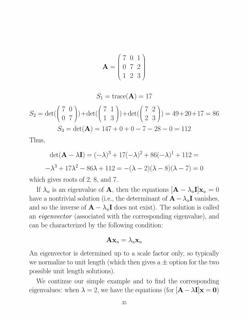
A =

⎛⎜⎜⎜⎜⎜⎝

7 0 1

0 7 2

1 2 3

⎞⎟⎟⎟⎟⎟⎠

S1 = trace(A) = 17

S2 = det(

⎛⎜⎝ 7 0

0 7

⎞⎟⎠)+det(

⎛⎜⎝ 7 1

1 3

⎞⎟⎠)+det(

⎛⎜⎝ 7 2

2 3

⎞⎟⎠) = 49+20+17 = 86

S3 = det(A) = 147 + 0 + 0 − 7 − 28 − 0 = 112

Thus,

det(A− λI) = (−λ)3 + 17(−λ)2 + 86(−λ)1 + 112 =

−λ3 + 17λ2 − 86λ + 112 = −(λ − 2)(λ − 8)(λ − 7) = 0

which gives roots of 2, 8, and 7.

If λu is an eigenvalue of A, then the equations [A − λuI]xu = 0

have a nontrivial solution (i.e., the determinant of A−λuI vanishes,

and so the inverse of A− λuI does not exist). The solution is called

an eigenvector (associated with the corresponding eigenvalue), and

can be characterized by the following condition:

Axu = λuxu

An eigenvector is determined up to a scale factor only, so typically

we normalize to unit length (which then gives a ± option for the two

possible unit length solutions).

We continue our simple example and to find the corresponding

eigenvalues: when λ = 2, we have the equations (for [A−λI]x = 0)

35

⎛⎜⎜⎜⎜⎜⎝

5 0 1

0 5 2

1 2 1

⎞⎟⎟⎟⎟⎟⎠

⎛⎜⎜⎜⎜⎜⎝

x1

x2

x3

⎞⎟⎟⎟⎟⎟⎠ =

⎛⎜⎜⎜⎜⎜⎝

0

0

0

⎞⎟⎟⎟⎟⎟⎠

with an arbitrary solution of⎛⎜⎜⎜⎜⎜⎝

−15a

−25a

a

⎞⎟⎟⎟⎟⎟⎠

Choosing a to be + 5√30

to obtain one of the two possible normalized

solutions, we have as our final eigenvector for λ = 2:⎛⎜⎜⎜⎜⎜⎜⎝

− 1√30

− 2√305√30

⎞⎟⎟⎟⎟⎟⎟⎠

For λ = 7 we will use the normalized eigenvector of⎛⎜⎜⎜⎜⎜⎝

− 2√5

1√5

0

⎞⎟⎟⎟⎟⎟⎠

and for λ = 8,⎛⎜⎜⎜⎜⎜⎜⎝

1√6

2√6

1√6

⎞⎟⎟⎟⎟⎟⎟⎠

One of the interesting properties of eigenvalues/eigenvectors for a

symmetric matrix A is that if λu and λv are distinct eigenvalues,

36

then the corresponding eigenvectors, xu and xv, are orthogonal (i.e.,

x′uxv = 0). We can show this in the following way: the defining

conditions of

Axu = λuxu

Axv = λvxv

lead to

x′vAxu = x′

vλuxu

x′uAxv = x′

uλvxv

Because A is symmetric and the left-hand-sides of these two expres-

sions are equal (they are one-by-one matrices and equal to their own

transposes), the right-hand-sides must also be equal. Thus,

x′vλuxu = x′

uλvxv ⇒

x′vxuλu = x′

uxvλv

Due to the equality of x′vxu and x′

uxv, and by assumption, λu �= λv,

the inner product x′vxu must be zero for the last displayed equality

to hold.

In summary of the above discussion, for every real symmetric ma-

trix AU×U , there exists an orthogonal matrix P (i.e., P′P = PP′ =

I) such that P′AP = D, where D is a diagonal matrix containing

the eigenvalues of A, and

P =(p1 . . . pU

)

37

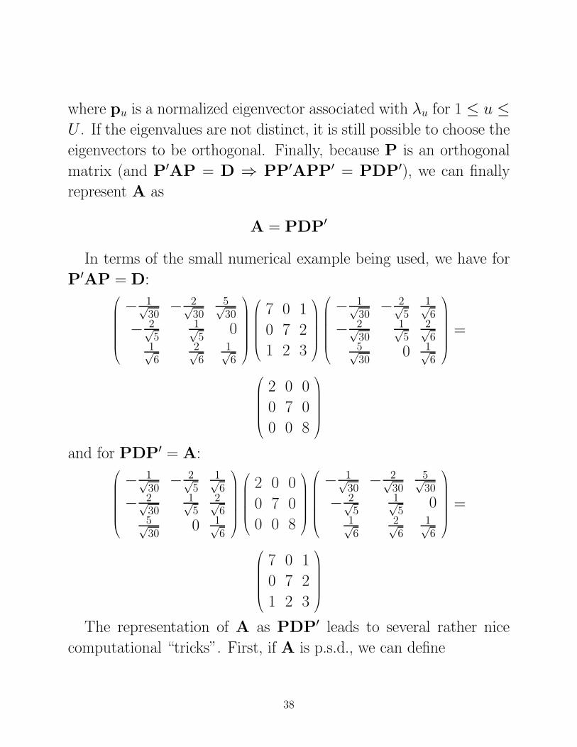
where pu is a normalized eigenvector associated with λu for 1 ≤ u ≤U . If the eigenvalues are not distinct, it is still possible to choose the

eigenvectors to be orthogonal. Finally, because P is an orthogonal

matrix (and P′AP = D ⇒ PP′APP′ = PDP′), we can finally

represent A as

A = PDP′

In terms of the small numerical example being used, we have for

P′AP = D:⎛⎜⎜⎜⎜⎜⎜⎝

− 1√30

− 2√30

5√30

− 2√5

1√5

01√6

2√6

1√6

⎞⎟⎟⎟⎟⎟⎟⎠

⎛⎜⎜⎜⎜⎜⎝

7 0 1

0 7 2

1 2 3

⎞⎟⎟⎟⎟⎟⎠

⎛⎜⎜⎜⎜⎜⎜⎝

− 1√30

− 2√5

1√6

− 2√30

1√5

2√6

5√30

0 1√6

⎞⎟⎟⎟⎟⎟⎟⎠

=

⎛⎜⎜⎜⎜⎜⎝

2 0 0

0 7 0

0 0 8

⎞⎟⎟⎟⎟⎟⎠

and for PDP′ = A:⎛⎜⎜⎜⎜⎜⎜⎝

− 1√30

− 2√5

1√6

− 2√30

1√5

2√6

5√30

0 1√6

⎞⎟⎟⎟⎟⎟⎟⎠

⎛⎜⎜⎜⎜⎜⎝

2 0 0

0 7 0

0 0 8

⎞⎟⎟⎟⎟⎟⎠

⎛⎜⎜⎜⎜⎜⎜⎝

− 1√30

− 2√30

5√30

− 2√5

1√5

01√6

2√6

1√6

⎞⎟⎟⎟⎟⎟⎟⎠

=

⎛⎜⎜⎜⎜⎜⎝

7 0 1

0 7 2

1 2 3

⎞⎟⎟⎟⎟⎟⎠

The representation of A as PDP′ leads to several rather nice

computational “tricks”. First, if A is p.s.d., we can define

38

D1/2 ≡⎛⎜⎜⎜⎜⎜⎝

√λ1 . . . 0... . . . ...

0 . . .√

λU

⎞⎟⎟⎟⎟⎟⎠

and represent A as

A = PD1/2D1/2P′ = PD1/2(PD1/2)′ = LL′, say.

In other words, we have “factored” A into LL′, for

L = PD1/2 =( √

λ1p1

√λ2p2 . . .

√λUpU

)

Secondly, if A is p.d., we can define

D−1 ≡⎛⎜⎜⎜⎜⎜⎝

1λ1

. . . 0... . . . ...

0 . . . 1λU

⎞⎟⎟⎟⎟⎟⎠

and represent A−1 as

A−1 = PD−1P′

To verify,

AA−1 = (PDP′)(PD−1P′) = I

Thirdly, to define a “square root” matrix, let A1/2 ≡ PD1/2P′. To

verify, A1/2A1/2 = PDP′ = A.

There is a generally interesting way to represent the multiplication

of two matrices considered as collections of column and row vectors,

respectively, where the final answer is a sum of outer products of

vectors. This view will prove particularly useful in our discussion of

39

principal component analysis. Suppose we have two matrices BU×V ,

represented as a collection of its V columns:

B =(b1 b2 . . . bV

)

and CV ×W , represented as a collection of its V rows:

C =

⎛⎜⎜⎜⎜⎜⎜⎜⎜⎝

c′1c′2...

c′V

⎞⎟⎟⎟⎟⎟⎟⎟⎟⎠

The product BC = D can be written as

BC =(b1 b2 . . . bV

)⎛⎜⎜⎜⎜⎜⎜⎜⎜⎝

c′1c′2...

c′V

⎞⎟⎟⎟⎟⎟⎟⎟⎟⎠

=

b1c′1 + b2c

′2 + · · · + bV c′V = D

As an example, consider the spectral decomposition of A consid-

ered above as PDP′, and where from now on, without loss of any gen-

erality, the diagonal entries in D are ordered as λ1 ≥ λ2 ≥ · · · ≥ λU .

We can represent A as

AU×U =( √

λ1p1 . . .√

λUpU

)⎛⎜⎜⎜⎜⎜⎝

√λ1p

′1

...√λUp′

U

⎞⎟⎟⎟⎟⎟⎠ =

λ1p1p′1 + · · · + λUpUp′

U

If A is p.s.d. and of rank R, then the above sum obviously stops at

R components. In general, the matrix BU×U that is a rank K (≤ R)

40

least-squares approximation to A can be given by

B = λ1p1p′1 + · · · + λkpKp′

K

and the value of the loss function:U∑

v=1

U∑u=1

(auv − buv)2 = (λ2

K+1 + · · · + λ2U)

12

0.3 The Singular Value Decomposition of a Matrix

The singular value decomposition (SVD) or the basic structure

of a matrix refers to the representation of any rectangular U × V

matrix, say, A, as a triple product:

AU×V = PU×RΔR×RQ′R×V

where the R columns of P are orthonormal; the R rows of Q′ are

orthonormal; Δ is diagonal with ordered positive entries, δ1 ≥ δ2 ≥· · · ≥ δR > 0; and R is the rank of A. Or, alternatively, we can “fill

up” this decomposition as

AU×V = P∗U×UΔ∗

U×V Q∗′V ×V

where the columns of P∗ and rows of Q∗′ are still orthonormal, and

the diagonal matrix Δ forms the upper-left-corner of Δ∗:

Δ∗ =

⎛⎜⎝ Δ ∅

∅ ∅⎞⎟⎠

here, ∅ represents an appropriately dimensioned matrix of all zeros.

In analogy to the least-squares result of the last section, if a rank K

(≤ R) matrix approximation to A is desired, say BU×V , the first K

ordered entries in Δ are taken:

41

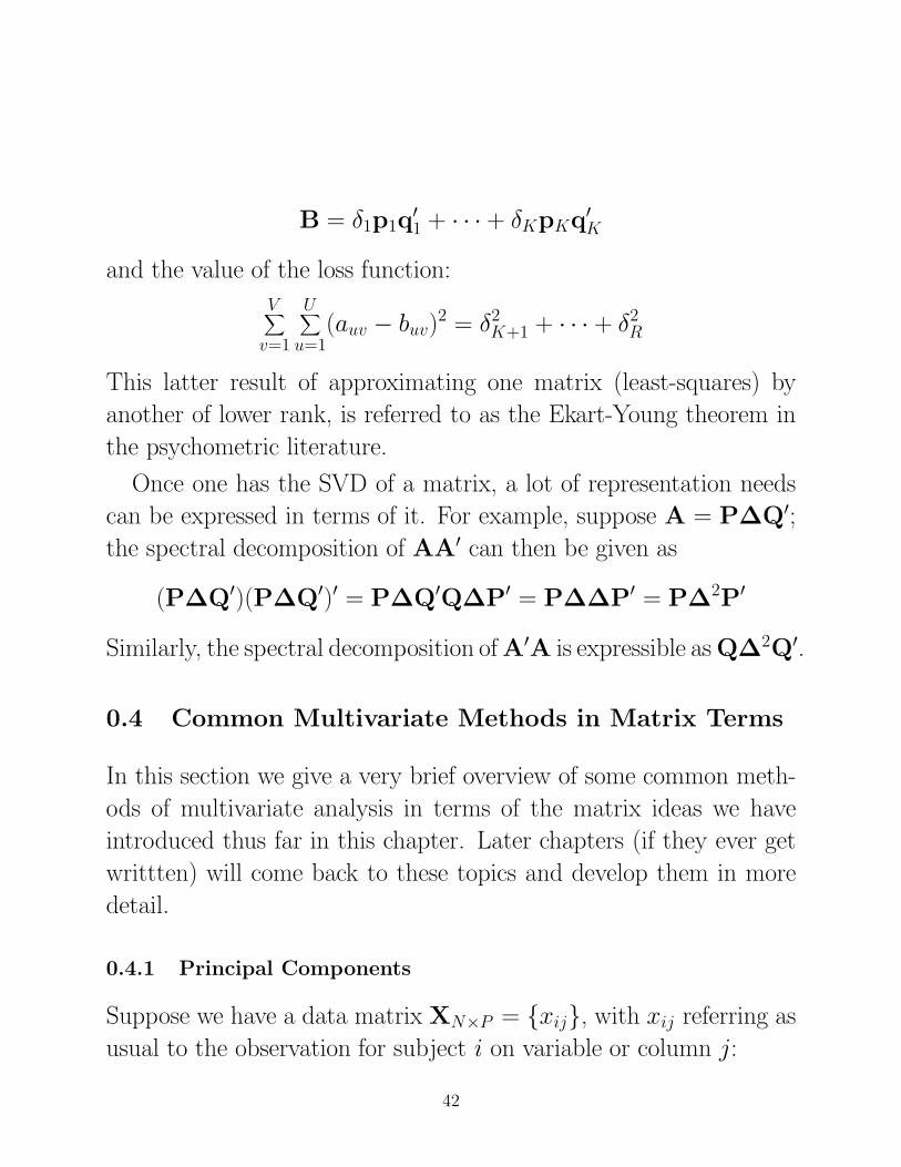
B = δ1p1q′1 + · · · + δKpKq′

K

and the value of the loss function:

V∑v=1

U∑u=1

(auv − buv)2 = δ2

K+1 + · · · + δ2R

This latter result of approximating one matrix (least-squares) by

another of lower rank, is referred to as the Ekart-Young theorem in

the psychometric literature.

Once one has the SVD of a matrix, a lot of representation needs

can be expressed in terms of it. For example, suppose A = PΔQ′;the spectral decomposition of AA′ can then be given as

(PΔQ′)(PΔQ′)′ = PΔQ′QΔP′ = PΔΔP′ = PΔ2P′

Similarly, the spectral decomposition of A′A is expressible as QΔ2Q′.

0.4 Common Multivariate Methods in Matrix Terms

In this section we give a very brief overview of some common meth-

ods of multivariate analysis in terms of the matrix ideas we have

introduced thus far in this chapter. Later chapters (if they ever get

writtten) will come back to these topics and develop them in more

detail.

0.4.1 Principal Components

Suppose we have a data matrix XN×P = {xij}, with xij referring as

usual to the observation for subject i on variable or column j:

42

XN×P =

⎛⎜⎜⎜⎜⎜⎜⎜⎜⎝

x11 x12 · · · x1P

x21 x22 · · · x2P... ... . . . ...

xN1 xN2 · · · xNP

⎞⎟⎟⎟⎟⎟⎟⎟⎟⎠

The columns can be viewed as containing N observations on each of

P random variables that we denote generically by X1, X2, . . . , XP .

We let A denote the P×P sample covariance matrix obtained among

the variables from X, and let λ1 ≥ · · · ≥ λP ≥ 0 be its P eigenvalues

and p1, . . . ,pP the corresponding normalized eigenvectors. Then,

the linear combination

p′k

⎛⎜⎜⎜⎜⎜⎝

X1...

XP

⎞⎟⎟⎟⎟⎟⎠

is called the kth (sample) principal component.

There are (at least) two interesting properties of principal compo-

nents to bring up at this time:

A) The kth principal component has maximum variance among

all linear combinations defined by unit length vectors orthogonal to

p1, . . . ,pk−1; also, it is uncorrelated with the components up to k−1;

B) A ≈ λ1p1p′1 + · · · + λKpKp′

K gives a least-squares rank K

approximation to A (a special case of the Ekart-Young theorem for

an arbitrary symmetric matrix).

0.4.2 Discriminant Analysis

Suppose we have a one-way analysis-of-variance (ANOVA) layout

with J groups (nj subjects in group j, 1 ≤ j ≤ J), and P measure-

43

ments on each subject. If xijk denotes person i, in group j, and the

observation of variable k (1 ≤ i ≤ nj; 1 ≤ j ≤ J ; 1 ≤ k ≤ P ), then

define the Between-Sum-of-Squares matrix

BP×P = { J∑j=1

nj(x·jk − x··k)(x·jk′ − x··k′)}P×P

and the Within-Sum-of-Squares matrix

WP×P = { J∑j=1

nj∑i=1

(xijk − x·jk)(xijk′ − x·jk′)}P×P

For the matrix product W−1B, let λ1, . . . , λT ≥ 0 be the eigen-

vectors (T = min(P, J − 1), and p1, . . . ,pT the corresponding nor-

malized eigenvectors. Then, the linear combination

p′k

⎛⎜⎜⎜⎜⎜⎝

X1...

XP

⎞⎟⎟⎟⎟⎟⎠

is called the kth discriminant function. It has the valuable property

of maximizing the univariate F -ratio subject to being uncorrelated

with the earlier linear combinations. A variety of applications of

discriminant functions exists in classification that we will come back

to later. Also, standard multivariate ANOVA significance testing is

based on various functions of the eigenvalues λ1, . . . , λT and their

derived sampling distributions.

0.4.3 Canonical Correlation

Suppose the collection of P random variables that we have observed

over the N subjects is actually in the form of two “batteries”, X1, . . . , XQ

44

and XQ+1, . . . , XP , and the observed covariance matrix AP×P is par-

titioned into four parts:

AP×P =

⎛⎜⎝ A11 A12

A′12 A22

⎞⎟⎠

where A11 is Q×Q and represents the observed covariances among

the variables in the first battery; A22 is (P − Q) × (P − Q) and

represents the observed covariances among the variables in the second

battery; A12 is Q× (P −Q) and represents the observed covariances

between the variables in the first and second batteries. Consider the

following two equations in unknown vectors a and b, and unknown

scalar λ:

A−111 A12A

−122 A′

12a = λa

A−122 A′

12A−111 A12b = λb

There are T solutions to these expressions (for T = min(Q, (P −Q))), given by normalized unit-length vectors, a1, . . . , aT and b1, . . . ,bT ;

and a set of common λ1 ≥ · · · ≥ λT ≥ 0.

The linear combinations of the first and second batteries defined

by ak and bk are the kth canonical variates and have squared cor-

relation of λk; they are uncorrelated with all other canonical variates

(defined either in the first or second batteries). Thus, a1 and b1

are the first canonical variates with squared correlation of λ1; among

all linear combinations defined by unit-length vectors for the vari-

ables in the two batteries, this squared correlation is the highest it

can be. (We note that the coefficient matrices A−111 A12A

−122 A′

12 and

A−122 A′

12A−111 A12 are not symmetric; thus, special symmetrizing and

45

equivalent equation systems are typically used to obtain the solutions

to the original set of expressions.)

0.4.4 Algebraic Restrictions on Correlations

A matrix AP×P that represents a covariance matrix among a collec-

tion of random variables, X1, . . . , XP is p.s.d.; and conversely, any

p.s.d. matrix represents the covariance matrix for some collection of

random variables. We partition A to isolate its last row and column

as

A =

⎛⎜⎝ B(P−1)×(P−1) g(P−1)×1

g′ aPP

⎞⎟⎠

B is the (P − 1) × (P − 1) covariance matrix among the variables

X1, . . . , XP−1; g is (P − 1) × 1 and contains the cross-covariance

between the the first P −1 variables and the P th; aPP is the variance

for the P th variable.

Based on the observation that determinants of p.s.d. matrices are

nonnegative, and a result on expressing determinants for partitioned

matrices (that we do not give here), it must be true that

g′B−1g ≤ aPP

or if we think correlations rather than merely covariances (so the

main diagonal of A consists of all ones):

g′B−1g ≤ 1

Given the correlation matrix B, the possible values the correlations

in g could have are in or on the ellipsoid defined in P −1 dimensions

by g′B−1g ≤ 1. The important point is that we do not have a “box”

46

in P − 1 dimensions containing the correlations with sides extending

the whole range of ±1; instead, some restrictions are placed on the

observable correlations that gets defined by the size of the correlation

in B. For example, when P = 3, a correlation between variables

X1 and X2 of r12 = 0 gives the “degenerate” ellipse of a circle for

constraining the correlation values between X1 and X2 and the third

variable X3 (in a two-dimensional r13 versus r23 coordinate system);

for r12 = 1, the ellipse flattens to a line in this same two-dimensional

space.

Another algebraic restriction that can be seen immediately is based

on the formula for the partial correlation between two variables,

“holding the third constant”:

r12 − r13r23√(1 − r2

13)(1 − r223)

Bounding the above by ±1 (because it is a correlation) and “solving”

for r12, gives the algebraic upper and lower bounds of

r12 ≤ r13r23 +√(1 − r2

13)(1 − r223)

r13r23 −√(1 − r2

13)(1 − r223) ≤ r12

0.4.5 The Biplot

Let A = {aij} be an n × m matrix of rank r. We wish to find a

second matrix B = {bij} of the same size, n × m, but of rank t,

where t ≤ r, such that the least squares criterion,∑

i,j(aij − bij)2, is

as small as possible overall all matrices of rank t.

47

The solution is to first find the singular value decomposition of A

as UDV′, where U is n × r and has orthonormal columns, V is

m× r and has orthonormal columns, and D is r× r, diagonal, with

positive values d1 ≥ d2 ≥ · · · ≥ dr > 0 along the main diagonal.

Then, B is defined as U∗D∗V∗′, where we take the first t columns of

U and V to obtain U∗ and V∗, respectively, and the first t values,

d1 ≥ · · · ≥ dt, to form a diagonal matrix D∗.The approximation of A by a rank t matrix B, has been one mech-

anism for representing the row and column objects defining A in a

low-dimensional space of dimension t through what can be generi-

cally labeled as a biplot (the prefix “bi” refers to the representation

of both the row and column objects together in the same space).

Explicitly, the approximation of A and B can be written as

B = U∗D∗V∗′ = U∗D∗αD(1−α)V∗′ = PQ′ ,

where α is some chosen number between 0 and 1, P = U∗D∗α and

is n × t, Q = (D(1−α)V∗′)′ and is m × t.

The entries in P and Q define coordinates for the row and column

objects in a t-dimensional space that, irrespective of the value of α

chosen, have the following characteristic:

If a vector is drawn from the origin through the ith row point and

the m column points are projected onto this vector, the collection of

such projections is proportional to the ith row of the approximating

matrix B. The same is true for projections of row points onto vectors

from the origin through each of the column points.

48

0.4.6 The Procrustes Problem

Procrustes (the subduer), son of Poseidon, kept an inn benefiting

from what he claimed to be a wonderful all-fitting bed. He lopped off

excessive limbage from tall guests and either flattened short guests by

hammering or stretched them by racking. The victim fitted the bed

perfectly but, regrettably, died. To exclude the embarrassment of an

initially exact-fitting guest, variants of the legend allow Procrustes

two, different-sized beds. Ultimately, in a crackdown on robbers

and monsters, the young Theseus fitted Procrustes to his own bed.

(Gower and Dijksterhuis, 2004)

Suppose we have two matrices, X1 and X2, each considered (for

convenience) to be of the same size, n × p. If you wish, X1 and

X2 can be interpreted as two separate p-dimensional coordinate sets

for the same set of n objects. Our task is to match these two con-

figurations optimally, with the criterion being least-squares: find a

transformation matrix, Tp×p, such that ‖ X1T−X2 ‖ is minimized,

where ‖ · ‖ denotes the sum-of-squares of the incorporated matrix,

i.e., if A = {auv}, then ‖ A ‖ = trace(A′A) =∑

u,v a2uv. For conve-

nience, assume both X1 and X2 have been normalized so ‖ X1 ‖ =

‖ X2 ‖ = 1, and the columns of X1 and X2 have sums of zero.

Two results are central:

(a) When T is unrestricted, we have the multivariate multiple

regression solution

T∗ = (X′1X1)

−1X1X2 ;

(b) When T is orthogonal, we have the Schonemann solution done

for his thesis in the Quantitative Division at Illinois in 1965 (pub-

lished in Psychometrika in 1966):

49

for the SVD of X′2X1 = USV′, we let T∗ = VU′.

0.4.7 Matrix Rank Reduction

Lagrange’s Theorem (as inappropriately named by C. R. Rao, be-

cause it should really be attributed to Guttman) can be stated as

follows:

Let G be a nonnegative-definite (i.e., a symmetric positive semi-

definite) matrix of order n×n and of rank r > 0. Let B be of order

n×s and such that B′GB is non-singular. Then the residual matrix

G1 = G − GB(B′GB)−1B′G (1)

is of rank r − s and is nonnegative definite.

Intuitively, this theorem allows you to “take out” “factors” from a

covariance (or correlation) matrix.

0.4.8 Torgerson Metric Multidimensional Scaling

Let A be a symmetric matrix of order n × n. Suppose we want

to find a matrix B of rank 1 (of order n × n) in such a way that

the sum of the squared discrepancies between the elements of A and

the corresponding elements of B (i.e.,∑n

j=1∑n

i=1(aij − bij)2) is at a

minimum. It can be shown that the solution is B = λkk′ (so all

columns in B are multiples of k), where λ is the largest eigenvalue of

A and k is the corresponding normalized eigenvector. This theorem

can be generalized. Suppose we take the first r largest eigenvalues

and the corresponding normalized eigenvectors. The eigenvectors are

collected in an n×r matrix K = {k1, . . . ,kr} and the eigenvalues in

a diagonal matrix Λ. Then KΛK′ is an n× n matrix of rank r and

50

is a least-squares solution for the approximation of A by a matrix of

rank r. It is assumed, here, that the eigenvalues are all positive. If

A is of rank r by itself and we take the r eigenvectors for which the

eigenvalues are different from zero collected in a matrix K of order

n × r, then A = KΛK′. Note that A could also be represented by

A = LL′, where L = KΛ1/2 (we factor the matrix), or as a sum of

r n × n matrices — A = λ1k1k′1 + · · · + λrkrk

′r.

Metric Multidimensional Scaling – Torgerson’s Model (Gower’s

Principal Coordinate Analysis)

Suppose I have a set of n points that can be perfectly repre-

sented spatially in r dimensional space. The ith point has coordi-

nates (xi1, xi2, . . . , xir). If dij =√∑r

k=1(xik − xjk)2 represents the

Euclidean distance between points i and j, then

d∗ij =r∑

k=1xikxjk, where

d∗ij = −1

2(d2

ij − Ai − Bj + C); (2)

Ai = (1/n)n∑

j=1d2

ij;

Bj = (1/n)n∑

i=1d2

ij;

C = (1/n2)n∑

i=1

n∑j=1

d2ij.

Note that {d∗ij}n×n = XX′, where X is of order n × r and the

entry in the ith row and kth column is xik.

51

So, the Question: If I give you D = {dij}n×n, find me a set of

coordinates to do it. The Solution: Find D∗ = {d∗ij}, and take its

Spectral Decomposition. This is exact here.

To use this result to obtain a spatial representation for a set of

n objects given any “distance-like” measure, pij, between objects i

and j, we proceed as follows:

(a) Assume (i.e., pretend) the Euclidean model holds for pij.

(b) Define p∗ij from pij using (1).

(c) Obtain a spatial representation for p∗ij using a suitable value

for r, the number of dimensions (at most, r can be no larger than

the number of positive eigenvalues for {p∗ij}n×n):

{p∗ij} ≈ XX′

(d) Plot the n points in r dimensional space.

0.4.9 A Guttman Multidimensional Scaling Result

I. If B is a symmetric matrix of order n, having all its elements non-

negative, the following quadratic form defined by the matrix A must

be positive semi-definite:

∑i,j

bij(xi − xj)2 =

∑i,j

xiaijxj,

where

aij =

⎧⎪⎨⎪⎩

∑nk=1;k �=i bik (i = j)

−bij (i �= j)

If all elements of B are positive, then A is of rank n − 1, and has

one smallest eigenvalue equal to zero with an associated eigenvector

52

having all constant elements. Because all (other) eigenvectors must

be orthogonal to the constant eigenvector, the entries in these other

eigenvectors must sum to zero.

This Guttman result can be used for a method of multidimensional

scaling (mds), and is one that seems to get reinvented periodically

in the literature. Generally, this method has been used to provide

rational starting points in iteratively-defined nonmetric mds.

0.4.10 A Few General MATLAB Routines to Know About

For Eigenvector/Eigenvalue Decompositions:

[V,D] = eig(A), where A = VDV′, for A square; V is or-

thogonal and contains eigenvectors (as columns); D is diagonal and

contains the eigenvalues (ordered from smallest to largest).

For Singular Value Decompositions:

[U,S,V] = svd(B), where B = USV′; the columns of U and

the rows of V′ are orthonormal; S is diagonal and contains the non-

negative singular values (ordered from largest to smallest).

The help comments for the Procrustes routine in the Statistics

Toolbox are given verbatim below. Note the very general transfor-

mation provided in the form of a MATLAB Structure that involves

optimal rotation, translation, and scaling.

>> help procrustesPROCRUSTES Procrustes Analysis

D = PROCRUSTES(X, Y) determines a linear transformation (translation,reflection, orthogonal rotation, and scaling) of the points in thematrix Y to best conform them to the points in the matrix X. The"goodness-of-fit" criterion is the sum of squared errors. PROCRUSTESreturns the minimized value of this dissimilarity measure in D. D isstandardized by a measure of the scale of X, given by

53

sum(sum((X - repmat(mean(X,1), size(X,1), 1)).^2, 1))

i.e., the sum of squared elements of a centered version of X. However,if X comprises repetitions of the same point, the sum of squared errorsis not standardized.

X and Y are assumed to have the same number of points (rows), andPROCRUSTES matches the i’th point in Y to the i’th point in X. Pointsin Y can have smaller dimension (number of columns) than those in X.In this case, PROCRUSTES adds columns of zeros to Y as necessary.

[D, Z] = PROCRUSTES(X, Y) also returns the transformed Y values.

[D, Z, TRANSFORM] = PROCRUSTES(X, Y) also returns the transformationthat maps Y to Z. TRANSFORM is a structure with fields:

c: the translation componentT: the orthogonal rotation and reflection componentb: the scale component

That is, Z = TRANSFORM.b * Y * TRANSFORM.T + TRANSFORM.c.

Examples:

% Create some random points in two dimensionsn = 10;X = normrnd(0, 1, [n 2]);

% Those same points, rotated, scaled, translated, plus some noiseS = [0.5 -sqrt(3)/2; sqrt(3)/2 0.5]; % rotate 60 degreesY = normrnd(0.5*X*S + 2, 0.05, n, 2);

% Conform Y to X, plot original X and Y, and transformed Y[d, Z, tr] = procrustes(X,Y);plot(X(:,1),X(:,2),’rx’, Y(:,1),Y(:,2),’b.’, Z(:,1),Z(:,2),’bx’);

% Compute a procrustes solution that does not include scaling:trUnscaled.T = tr.T;trUnscaled.b = 1;trUnscaled.c = mean(X) - mean(Y) * trUnscaled.T;ZUnscaled = Y * trUnscaled.T + repmat(trUnscaled.c,n,1);dUnscaled = sum((ZUnscaled(:)-X(:)).^2) ...

/ sum(sum((X - repmat(mean(X,1),n,1)).^2, 1));

54