Multivariate Geostatistical Simulation using Principal ...

Annual Report 2019 Paper 2019-07

© Predictive Geometallurgy and Geostatistics Lab, Queen’s University 94

Multivariate Geostatistical Simulation using Principal Component Analysis1

Maria Bolgkoranou ([email protected])

Julian M. Ortiz ([email protected])

Abstract Multivariate geostatistical simulation is aimed at reproducing the statistical relationships between variables and their spatial distribution. We present a methodology whereby grades and a filler variable are transformed to log-ratios, to impose the sum to 100%. Then, these log-ratios are linearly transformed to Principal Components (PCs). Sequential Gaussian Simulation is performed and the simulated factors are then back-transformed to simulated log-ratios, and these are back-transformed to grades. An application to a Nickel laterite deposit is presented. Spatial dependences are checked by use of cross-variograms. This confirms that PCA tends to spatially decorrelate the factors, allowing for the independent simulation of each PCs, instead of requiring a co-simulation. The results of SGS showed that the simulated grades resulting from the proposed approach reproduce reasonably well the spatial and statistical relationships between the grades. Co-simulation of the log-ratios considering the spatial cross relationships between the variables using a linear model of coregionalization was performed and the results were compared with the back-transformed grades after Principal Component Analysis.

1. Introduction Multivariate geostatistics is used to take advantage of spatial relationships between variables, in order to improve the estimation of a variable using secondary variables, or to jointly simulate a set of correlated variables, preserving their relationships in the models.

There are many methods available to create multivariate models. Sequential Gaussian cosimulation requires a linear model of coregionalization (Verly, 1993), which imposes constraints into the modeling of the direct and cross-variograms, making it inflexible. Other approaches try to avoid this burden by simplifying the cross correlation model by using collocated co-kriging to infer the conditional distributions during simulation (Almeida and Journel, 1994), or by attempting to decorrelate the data through the use of minimum/maximum autocorrelation factors (Desbarats and Dimitrakopoulos, 2000), stepwise conditional transformation (Leuangthong and Deutsch, 2003), or diagonalization approximation (Mueller and Ferreira, 2012).

1 Cite as: Bolgkoranou M, Ortiz JM (2019) Multivariate geostatistical simulation using Principal Component Analysis, Predictive Geometallurgy and Geostatistics Lab, Queen’s University, Annual Report 2019, paper 2019-07, 94-117.


Principal Component Analysis (PCA) is one of the most commonly used methods for multivariate data analysis, due to its mathematical simplicity and to its simple interpretation (Wackernagel, 2003). A linear transformation takes place, in which a set of correlated variables are transformed into uncorrelated (orthogonal) factors (Hotelling 1933; Johnson and Wichern, 1982). The factorization occurs with collocated data, which does not necessarily remove the spatial correlation that may exist between non-collocated data, either from a single variable or between variables (Suro-Perez and Journel, 1991). PCA has been used in geology and soil science before and is a well-established technique in statistical analysis (Davis, 1986; Webster and Oliver, 1990; Goovaerts, 1997).

PCA can be used to reduce the co-kriging of N variables, into the kriging of N uncorrelated principal components (Davis and Greenes, 1983; Goovaerts, 1997). Furthermore, PCA can be used as a compression tool, if only the first few principal components are retained, reproducing most of the variability of the original variables (Wackernagel, 2003).

In this paper, we present a detailed methodology to apply PCA, as a simple decorrelation approach of a compositional dataset, and show its application and performance in a Nickel laterite deposit. The back-transformed grades after the simulation of the Principal Component Analysis were compared to the ones coming from the simulation of the log-ratios. Further validation of the results is performed by comparing the back-transformed grades coming from the simulation of the Principal Components with the back-transformed grades coming from the co-simulation of the log-ratios.

2. Notation In this paper, the original variable is successively transformed several times, so, we provide notation to help the reader:

𝑝 − 1 is the dimension of the original vector variable. 𝑝 is the dimension of the vector variable after adding the filler to complete 100%. 𝑛 is the number of data samples. 𝑋 is the (𝑝 − 1) dimensional vector with the original variable. 𝑋 is the (𝑝) dimensional vector with the original variable, including the filler variable. 𝑍 is the (𝑝 − 1) dimensional vector of additive log-ratios. 𝐹 is the (𝑝 − 1) dimensional vector of principal components computed from the log-ratios. 𝑌 is the (𝑝 − 1) dimensional vector of normal scores of the principal components computed from

the log-ratios.

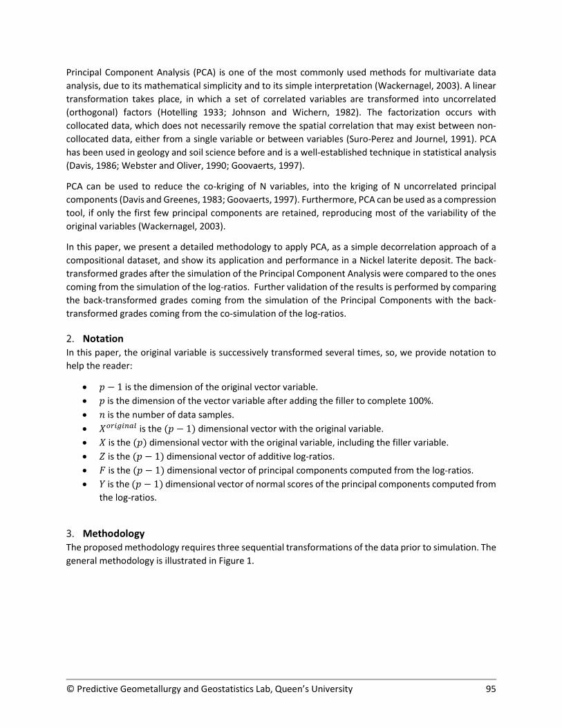
3. Methodology The proposed methodology requires three sequential transformations of the data prior to simulation. The general methodology is illustrated in Figure 1.


Figure 1: Flowchart of the proposed methodology.

The original variables are the grades (in %) from chemical analyses for a number of samples over the domain of interest. The original grades are noted as:

𝑋 (𝑢 ) = 𝑋 (𝑢 ), 𝑋 (𝑢 ), … , 𝑋 (𝑢 ) ∀𝛼 = 1, … , 𝑛 (1)

Since the grades form a composition, we need to complete the vector with a filler variable, to have the set of variables that sum to 100%:

𝑅(𝑢 ) = 100% − 𝑋 (𝑢 ) ∀𝛼 = 1, … , 𝑛 (2)

The vector needs to be updated, by adding the filler variable:

𝑋(𝑢 ) = 𝑋 (𝑢 ), 𝑋 (𝑢 ), … , 𝑋 (𝑢 ), 𝑅(𝑢 ) ∀𝛼 = 1, … , 𝑛 (3)

Notice that this approach requires all variables to be informed at all locations, that is, the dataset must be homotopic. Samples with missing variables are common in geological data sets for many reasons. The missing data must be imputed (inferred) to permit the measured data to be used to their full extent. Imputation methods for geological data should address spatial structure and multivariate complexity. If some variables are missing, an imputation process should be applied (Silva and Deutsch, 2016).

The methodology is general so that the transformation of log-ratios into factors can be done with any method. This opens possibilities to use diverse transformations available and check their effect. In this paper, we present the straightforward use of Principal Component Analysis (PCA) to perform a linear transformation, which significantly decorrelates the data.

3.1. Log-ratio transform Geological data are frequently reported in terms of the grades of different elements or the mineralogical proportions present in the rock. These sets of variables form a closed array or a composition, as their sum must add to the whole of the material. If all elements are considered, they should sum to 100%. If mineralogical proportions are used, they should add up to 1. This translates in a dependence between the variables, as there is always one less degree of freedom in the system, than variables available. Correlations are also distorted by this dependence, and this can lead to wrong inference and interpretations (Pawlowsky-Glahn and Olea, 2004). This also occurs with sub-compositions, that is when


only a subset of all the variables that form the composition are used (Pawlowsky-Glahn and Egozcue, 2006).

Considering the data {𝑋(𝑢 ), 𝛼 = 1, … , 𝑛} form a composition, compositional data analysis solves this closure problem by applying a log-ratio transformation of the data, so that any further statistical manipulation respects the constraint that the sum adds to 100% (Pawlowsky-Glahn and Egozcue, 2006).

The three most important transformations are:

1. Additive log-ratio (alr): it is the logarithm of the ratio between each component and one of the variables, in our case, the filler variable, and was introduced by Aitchison (1982) (see also Pawlowsky and Egozcue, 2006; Aitchison, 1986);

2. Centered log-ratio (clr): it is the logarithm of the ratio between each component and the geometric mean of the parts, and was also introduced by Aitchison (1982); and

3. Isometric log-ratio (ilr): it is obtained by projecting the composition over an orthonormal basis with (𝑝 − 1) dimensions. It was introduced by Egozcue et al. (2003).

In our methodology, we used the alr transform, therefore, the data are transformed to a new vector variable, as follows:

𝑍(𝑢 ) = 𝑙𝑜𝑔𝑋 (𝑢 )

𝑅(𝑢 ), 𝑙𝑜𝑔

𝑋 (𝑢 )

𝑅(𝑢 ), … , 𝑙𝑜𝑔

𝑋 (𝑢 )

𝑅(𝑢 ) ∀𝛼 = 1, … , 𝑛 (4)

The 𝑝 dimensional vector 𝑋(𝑢 ), becomes a (𝑝 − 1) dimensional vector 𝑍(𝑢 ).

3.2. Principal Component Transform The next step is to transform the log-ratios obtained in the previous step to linearly uncorrelated factors by using Principal Component Analysis. This principal component transformation finds a set of orthogonal linear axes that passes through the multivariate mean of the log-ratio transformed variables, and is such that the variance of the projections of the original log-ratios onto the first axis (called first principal component) is maximized. Axes corresponding to subsequent principal components are determined orthogonal to the previous ones, and with maximum variance (Howarth, 2017).

Principal components are found after an eigen-decomposition of the covariance matrix of the variable of interest (Wackernagel, 2003). The steps required are:

Compute the mean vector of the variables in vector 𝑍:

𝑚 = 𝑚 , 𝑚 , … , 𝑚 (5)

where:

𝑚 =1

𝑛𝑍 (𝑢 ) ∀𝑖 = 1, … , 𝑝 − 1 (6)

Calculate the covariance matrix:


𝐶 =1

𝑛(𝑍 − 𝑚) ∙ (𝑍 − 𝑚) (7)

Decompose the covariance through an eigen-decomposition: 𝐶 = 𝑄 ∙ Λ ∙ 𝑄 (8)

where 𝑄 is a matrix where the columns correspond to the eigen-vectors of 𝐶 , Λ is a diagonal matrix where the terms in the diagonal are the eigen-values of 𝐶 , sorted in decreasing order.

Determine the factors (principal components) 𝐹: the principal components are obtained by multiplying the data matrix by the eigen-vectors:

𝐹 = (𝑍 − 𝑚) ∙ 𝑄 (9)

Although the goal of PCA is to decompose the original variable into decorrelated components, notice that the data can be reconstructed from these principal components:

𝑍 = 𝐹 ∙ 𝑄 + 𝑚 (10)

The (𝑝 − 1) dimensional vector 𝑍(𝑢 ) becomes a (𝑝 − 1) dimensional vector 𝐹(𝑢 ). Data compression can be achieved in the last step of the process described above, by retaining only the first 𝑘 < (𝑝 − 1) principal components, that is, an approximate reconstruction is obtained as: 𝑍 = 𝐹 ∙ (𝑄 ) + 𝑚, where 𝐹 are the first 𝑘 principal components, and 𝑄 corresponds to the first 𝑘 columns of the matrix of eigen-vectors, hence, these are the eigen-vectors corresponding to the first 𝑘 highest eigen-values. In our case, compression was not used.

3.3. Normal Score Transform In order to spatially simulate the principal components, and assuming these are independent from each other, a multigaussian geostatistical simulation method can be used (Chiles and Delfiner, 2012). These methods require a normal score transformation to satisfy the requirement of gaussianity. Although in theory a multigaussian assumption is needed, in practice only the univariate condition is imposed through a quantile or polynomial transform.

For each component of the vector of principal component factors, a univariate transformation is performed as follows:

𝑌 = 𝜑 (𝐹 ) ∀𝑖 = 1, … , 𝑝 − 1 (11)

where 𝜑 is the transformation function for variable 𝑖.

3.4. Gaussian Simulation Variables transformed to normal scores can now be simulated using any of the available multigaussian simulation methods available in the geostatistical toolbox. The simulation can proceed independently for each variable 𝑌 , 𝑖 = 1, … , 𝑝 − 1, under the assumption that the normal scores of the principal components are independent, that is, their collocated values are linearly decorrelated and they do not show spatial correlation or non-linear correlation. This can be easily checked by plotting scatterplots and displaying the experimental direct and cross-variograms.

The simulation process will return as output a suite of 𝐿 realizations of the normal scores of the principal components, over a lattice of locations 𝑢 defined over the simulation domain 𝐷:


𝑌 , (𝑢), 𝑢 ∈ 𝐷 ∀𝑖 = 1, … , 𝑝 − 1; ∀𝑙 = 1, … , 𝐿 (12)

These realizations reproduce a histogram following a standard normal distribution, honor the normally-transformed data at sample locations (𝑌 (𝑢 ), ∀𝑖 = 1, … , 𝑝 − 1; ∀𝛼 = 1, … , 𝑛), and reproduce the spatial continuity imposed by the variogram model (Deutsch and Journel, 1998).

3.5. Back-transformations The resulting simulated values need to be brought back to their original units by applying the corresponding normal score, principal component and log-ratio back-transformations.

The first back-transformation brings the Gaussian simulated values back to principal components, by using the inverse of the transformation function for each principal component.

𝐹 , (𝑢) = 𝜑 𝑌 , (𝑢) (13)

The second back-transformation reconstructs simulated log-ratios, from the simulated principal component variables, at every location in the simulation lattice. These are obtained by multiplying the vector of simulated principal components by the transposed matrix of eigen-vectors and adding back the vector of means of the log-ratios.

𝑍 (𝑢) = 𝐹 (𝑢) ∙ 𝑄 + 𝑚 (14)

Finally, the third back-transformation brings the simulated vector of log-ratios, which is a 𝑝 − 1 dimensional vector, to the original grades, including the filler variable. This is achieved by determining the closure of the exponentials of the simulated log-ratios.

𝑋 (𝑢) = 𝑎𝑙𝑟 𝑍 (𝑢) = 𝒞 exp 𝑍 ; 0 (15)

4. Application to a Nickel-Laterite deposit

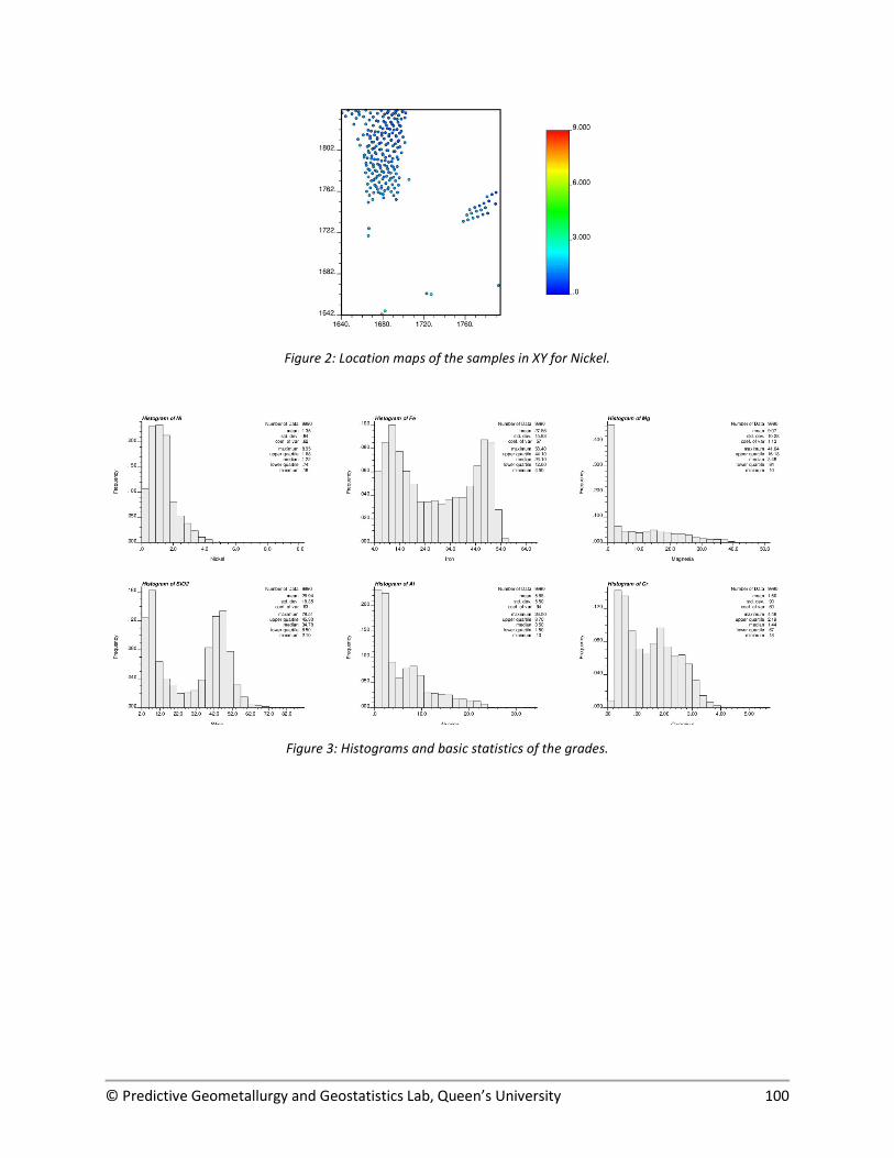
4.1. Proposed methodology: simulating PC transformed log-ratios Six geochemical variables corresponding to grades in % of a Nickel laterite deposit are available at 9990 locations in the database: 𝑋 = 𝑁𝑖; 𝑋 = 𝐹𝑒; 𝑋 = 𝑀𝑔𝑂; 𝑋 = 𝑆𝑖𝑂 ; 𝑋 = 𝐴𝑙 𝑂 ; 𝑋 = 𝐶𝑟. A filler variable 𝑅 = 100% − ∑ 𝑋 is calculated to ensure closure. Then, the additive log-ratios (alr) are computed with respect to the filler variable. Location maps of the samples are presented in Figure 2, as well as the basic statistics of the grades (Figure 3). Scatterplots between the log-ratios (for collocated locations) are shown in Figure 4.

Given that the data are preferentially sampled in specific areas, declustering is required to obtain the representative distribution of the grades (Pyrcz and Deutsch, 2003). Cell declustering is used to determine the weights associated to each sample, based on their location.

Principal component analysis is applied over the log-ratios.


Figure 2: Location maps of the samples in XY for Nickel.

Figure 3: Histograms and basic statistics of the grades.


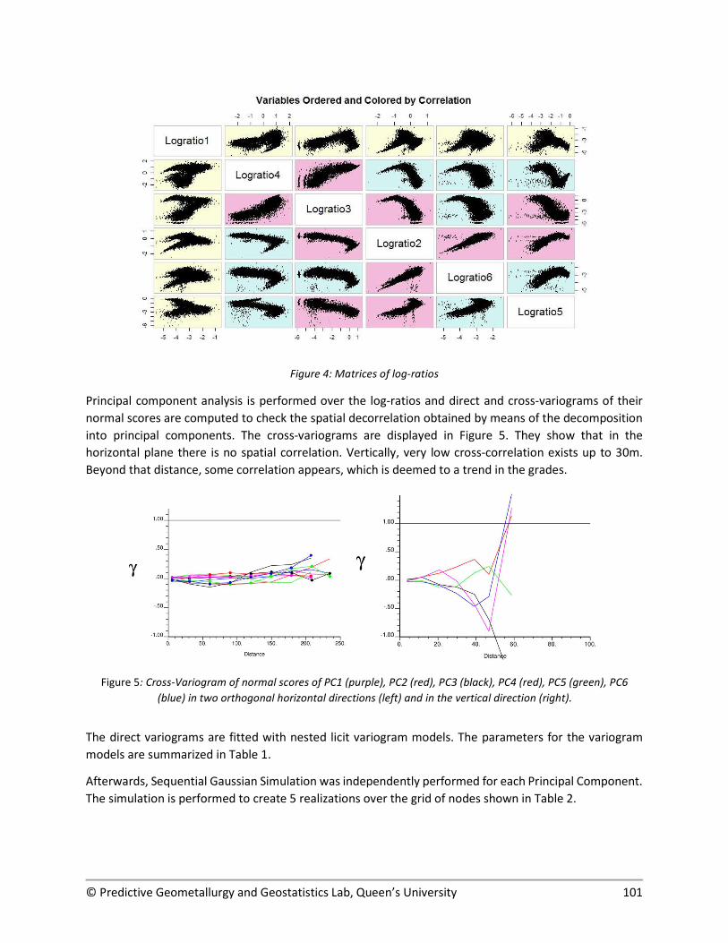
Figure 4: Matrices of log-ratios

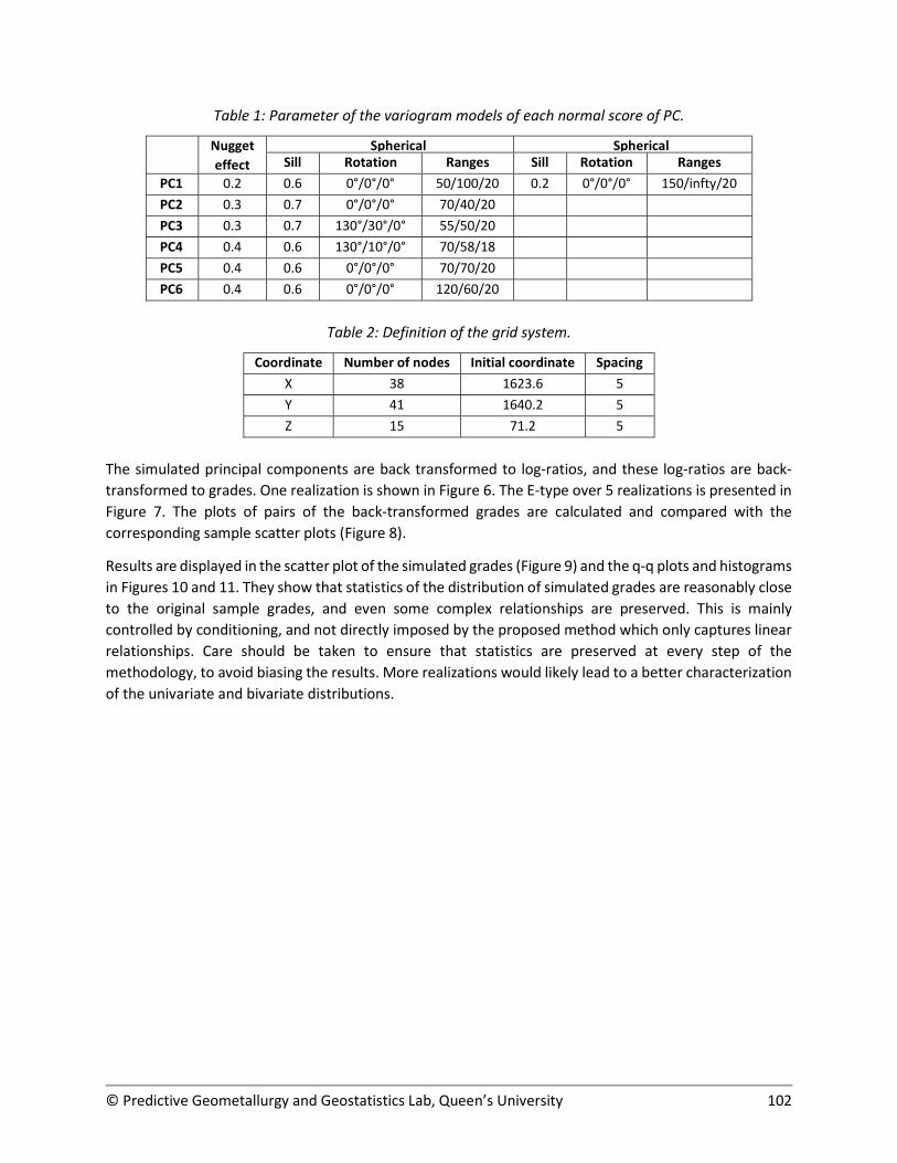
Principal component analysis is performed over the log-ratios and direct and cross-variograms of their normal scores are computed to check the spatial decorrelation obtained by means of the decomposition into principal components. The cross-variograms are displayed in Figure 5. They show that in the horizontal plane there is no spatial correlation. Vertically, very low cross-correlation exists up to 30m. Beyond that distance, some correlation appears, which is deemed to a trend in the grades.

Figure 5: Cross-Variogram of normal scores of PC1 (purple), PC2 (red), PC3 (black), PC4 (red), PC5 (green), PC6 (blue) in two orthogonal horizontal directions (left) and in the vertical direction (right).

The direct variograms are fitted with nested licit variogram models. The parameters for the variogram models are summarized in Table 1.

Afterwards, Sequential Gaussian Simulation was independently performed for each Principal Component. The simulation is performed to create 5 realizations over the grid of nodes shown in Table 2.


Table 1: Parameter of the variogram models of each normal score of PC.

Nugget effect

Spherical Spherical Sill Rotation Ranges Sill Rotation Ranges

PC1 0.2 0.6 0°/0°/0° 50/100/20 0.2 0°/0°/0° 150/infty/20 PC2 0.3 0.7 0°/0°/0° 70/40/20 PC3 0.3 0.7 130°/30°/0° 55/50/20 PC4 0.4 0.6 130°/10°/0° 70/58/18 PC5 0.4 0.6 0°/0°/0° 70/70/20 PC6 0.4 0.6 0°/0°/0° 120/60/20

Table 2: Definition of the grid system.

Coordinate Number of nodes Initial coordinate Spacing X 38 1623.6 5 Y 41 1640.2 5 Z 15 71.2 5

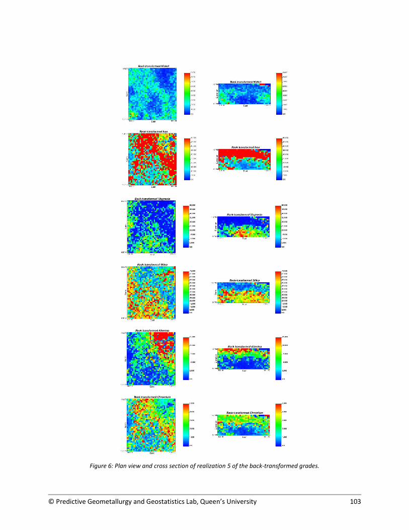
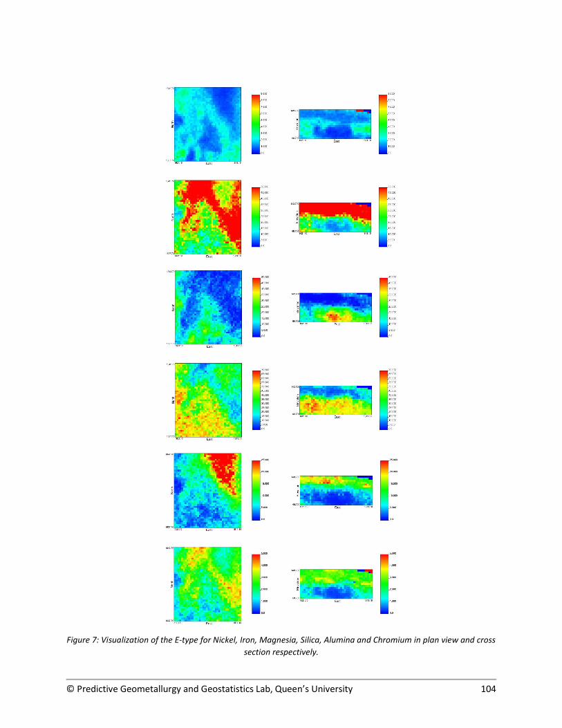
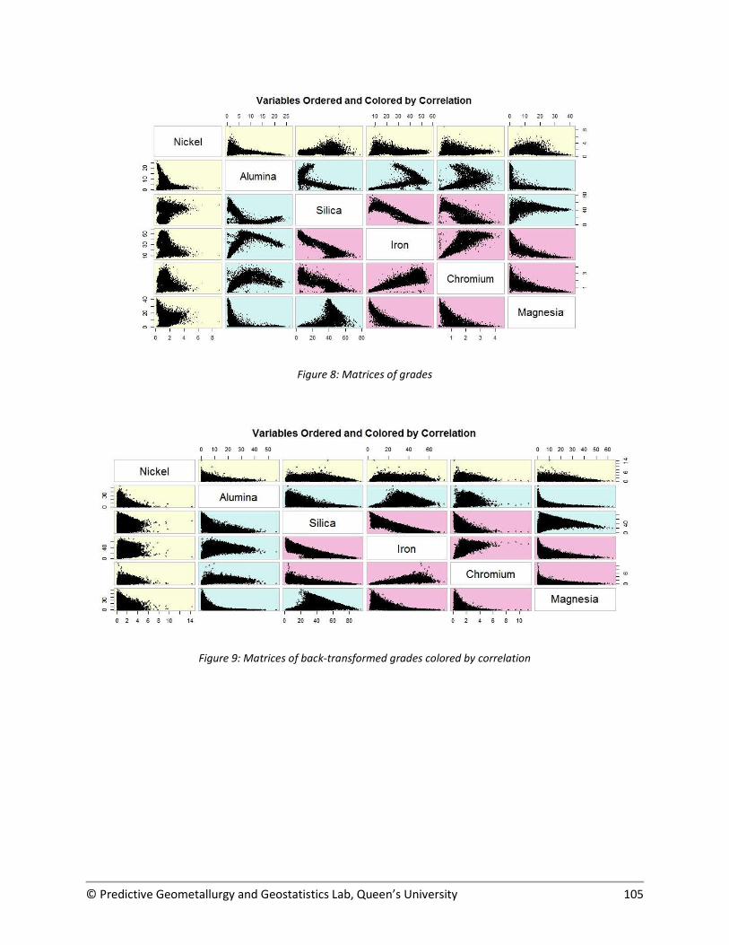
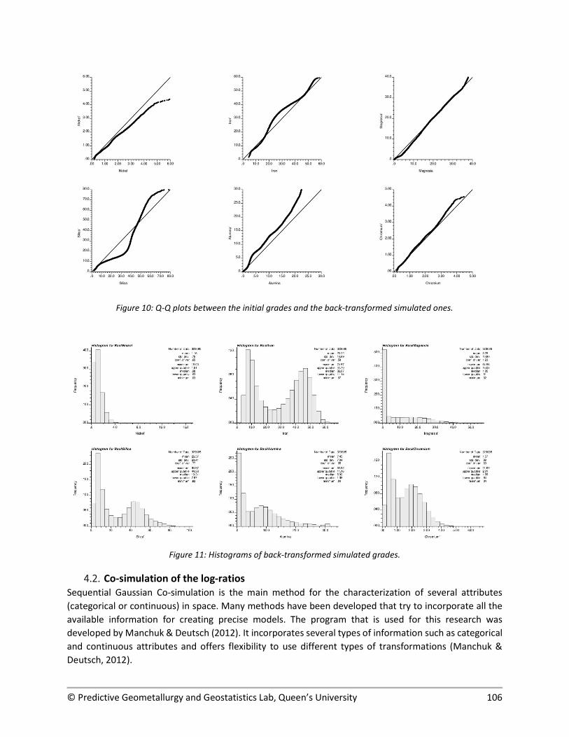
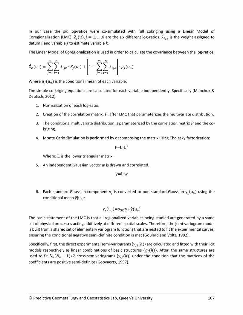
The simulated principal components are back transformed to log-ratios, and these log-ratios are back-transformed to grades. One realization is shown in Figure 6. The E-type over 5 realizations is presented in Figure 7. The plots of pairs of the back-transformed grades are calculated and compared with the corresponding sample scatter plots (Figure 8).

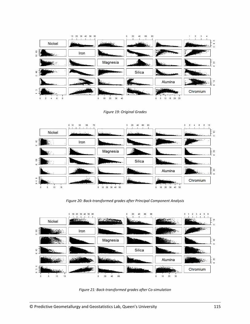
Results are displayed in the scatter plot of the simulated grades (Figure 9) and the q-q plots and histograms in Figures 10 and 11. They show that statistics of the distribution of simulated grades are reasonably close to the original sample grades, and even some complex relationships are preserved. This is mainly controlled by conditioning, and not directly imposed by the proposed method which only captures linear relationships. Care should be taken to ensure that statistics are preserved at every step of the methodology, to avoid biasing the results. More realizations would likely lead to a better characterization of the univariate and bivariate distributions.


Figure 6: Plan view and cross section of realization 5 of the back-transformed grades.


Figure 7: Visualization of the E-type for Nickel, Iron, Magnesia, Silica, Alumina and Chromium in plan view and cross section respectively.


Figure 8: Matrices of grades

Figure 9: Matrices of back-transformed grades colored by correlation


Figure 10: Q-Q plots between the initial grades and the back-transformed simulated ones.

Figure 11: Histograms of back-transformed simulated grades.

4.2. Co-simulation of the log-ratios Sequential Gaussian Co-simulation is the main method for the characterization of several attributes (categorical or continuous) in space. Many methods have been developed that try to incorporate all the available information for creating precise models. The program that is used for this research was developed by Manchuk & Deutsch (2012). It incorporates several types of information such as categorical and continuous attributes and offers flexibility to use different types of transformations (Manchuk & Deutsch, 2012).


In our case the six log-ratios were co-simulated with full cokriging using a Linear Model of Coregionalization (LMC). 𝑍 (𝑢), 𝑗 = 1, … ,6 are the six different log-ratios. 𝜆 is the weight assigned to datum 𝑖 and variable 𝑗 to estimate variable 𝑘.

The Linear Model of Coregionalization is used in order to calculate the covariance between the log-ratios.

𝑍 (𝑢 ) = 𝜆 ∙ 𝑍 (𝑢 ) + 1 − 𝜆 ∙ 𝜇 (𝑢 )

Where 𝜇 (𝑢 ) is the conditional mean of each variable.

The simple co-kriging equations are calculated for each variable independently. Specifically (Manchuk & Deutsch, 2012):

1. Normalization of each log-ratio.

2. Creation of the correlation matrix, 𝑃, after LMC that parameterizes the multivariate distribution.

3. The conditional multivariate distribution is parameterized by the correlation matrix 𝑃 and the co-kriging.

4. Monte Carlo Simulation is performed by decomposing the matrix using Cholesky factorization:

P=L∙LT

Where: L is the lower triangular matrix.

5. An independent Gaussian vector 𝑤 is drawn and correlated.

y=L∙w

6. Each standard Gaussian component ys is converted to non-standard Gaussian ys(uo) using the conditional mean y(uo):

ys(uo)=σSK∙y+y(uo)

The basic statement of the LMC is that all regionalized variables being studied are generated by a same set of physical processes acting additively at different spatial scales. Therefore, the joint variogram model is built from a shared set of elementary variogram functions that are nested to fit the experimental curves, ensuring the conditional negative semi-definite condition is met (Goulard and Voltz, 1992).

Specifically, first, the direct experimental semi-variograms (𝛾 (ℎ)) are calculated and fitted with their licit models respectively as linear combinations of basic structures (𝑔 (ℎ)). After, the same structures are used to fit 𝑁 (𝑁 − 1)/2 cross-semivariograms (𝛾 (ℎ)) under the condition that the matrices of the coefficients are positive semi-definite (Goovaerts, 1997).


Table 1: Parameter of the direct variogram models of each normal score of log-ratio:

Nugget Effect

Spherical

Sill Rotation Ranges

Log-ratio1 0.4 0.6 140°/-20°/0° 70/90/20

Log-ratio2 0.2 0.8 140°/-20°/0° 70/90/20

Log-ratio3 0.2 0.8 140°/-20°/0° 70/90/20

Log-ratio4 0.3 0.7 140°/-20°/0° 70/90/20

Log-ratio5 0.3 0.7 140°/-20°/0° 70/90/20

Log-ratio6 0.3 0.7 140°/-20°/0° 70/90/20

Table 2: Parameter of the cross-variogram models of each normal score of log-ratio:

Nugget Effect

Spherical

Sill Rotation Ranges

Log-ratio1-Log-ratio2 0 0.2 140°/-20°/0° 70/90/20



Log-ratio1-Log-ratio5 0 -0.15 140°/-20°/0° 70/90/20





Log-ratio2-Logratio6 0.2 0.7 140°/-20°/0° 70/90/20


Log-ratio3-Log-ratio5 -0.1 -0.7 140°/-20°/0° 70/90/20

Log-ratio3-Log-ratio6 -0.1 -0.5 140°/-20°/0° 70/90/20



Log-ratio5-Log-ratio6 0.15 0.6 140°/-20°/0° 70/90/20


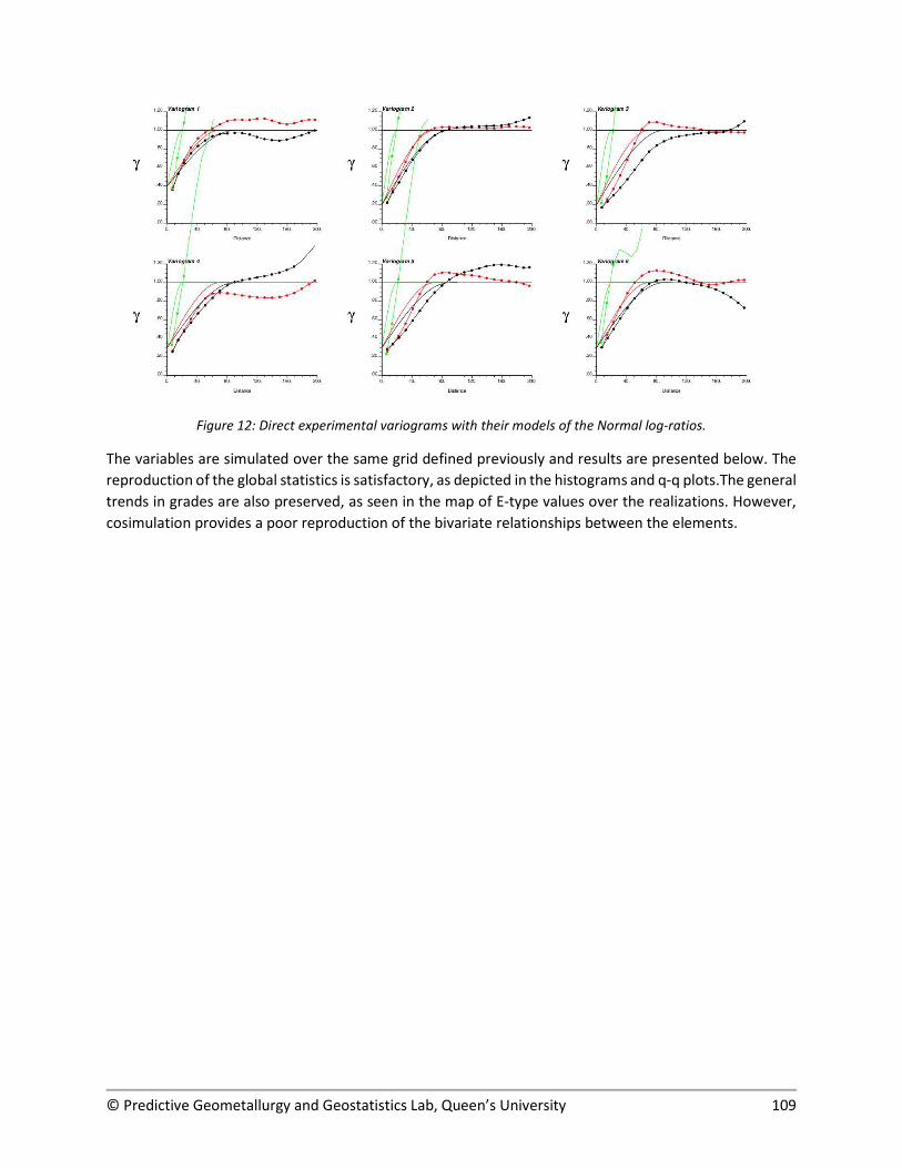
Figure 12: Direct experimental variograms with their models of the Normal log-ratios.

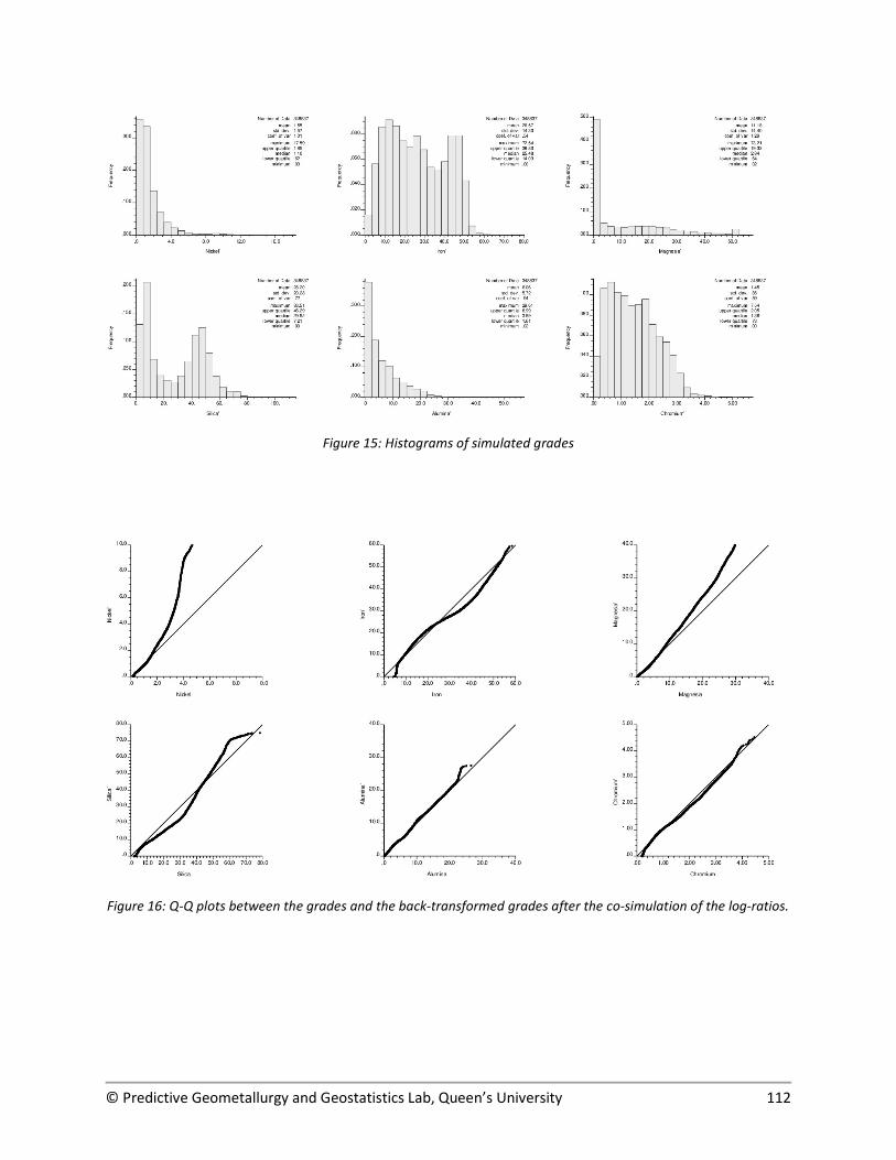
The variables are simulated over the same grid defined previously and results are presented below. The reproduction of the global statistics is satisfactory, as depicted in the histograms and q-q plots.The general trends in grades are also preserved, as seen in the map of E-type values over the realizations. However, cosimulation provides a poor reproduction of the bivariate relationships between the elements.


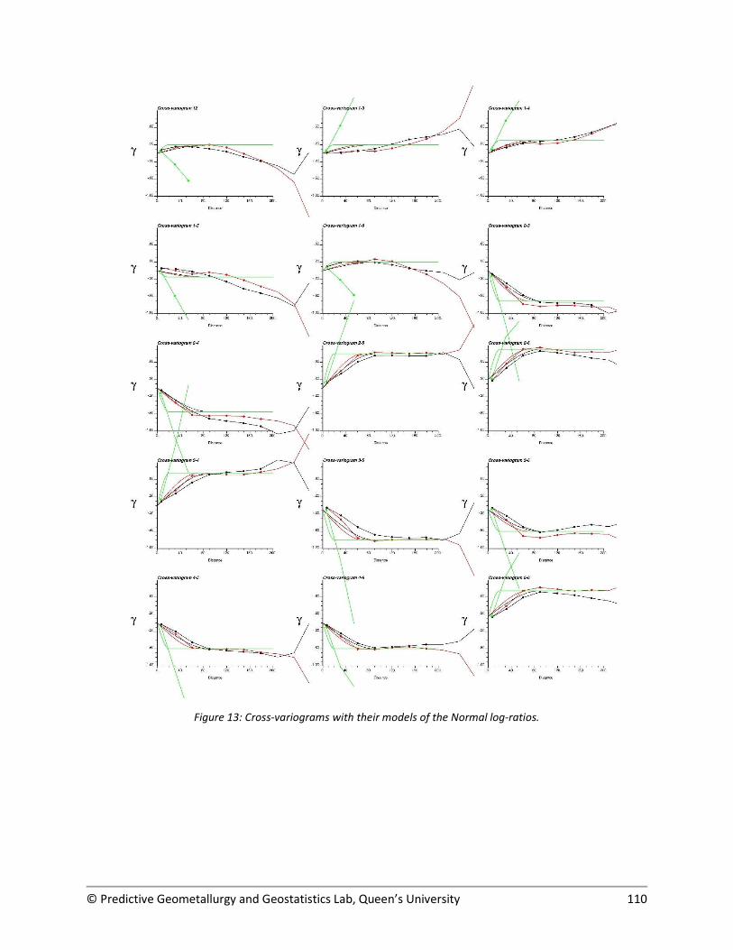
Figure 13: Cross-variograms with their models of the Normal log-ratios.


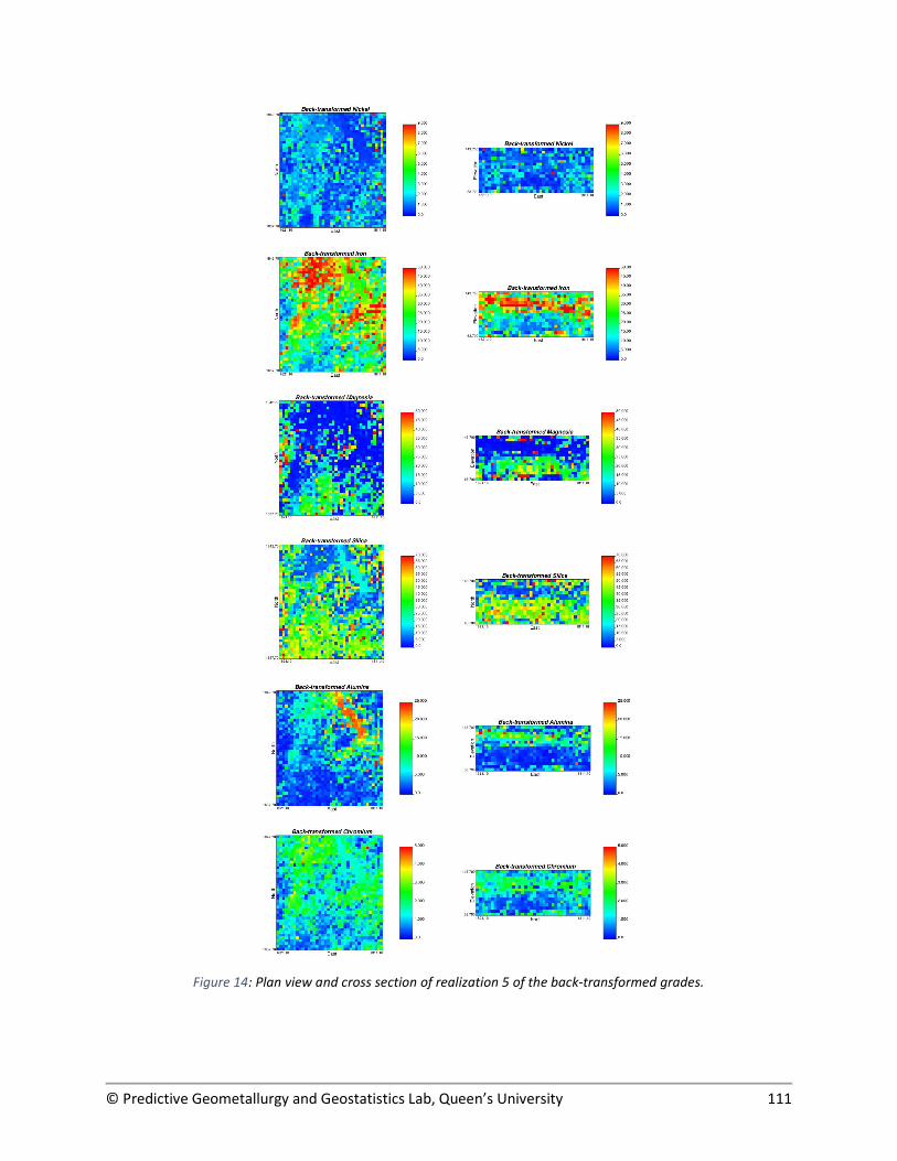
Figure 14: Plan view and cross section of realization 5 of the back-transformed grades.


Figure 15: Histograms of simulated grades

Figure 16: Q-Q plots between the grades and the back-transformed grades after the co-simulation of the log-ratios.


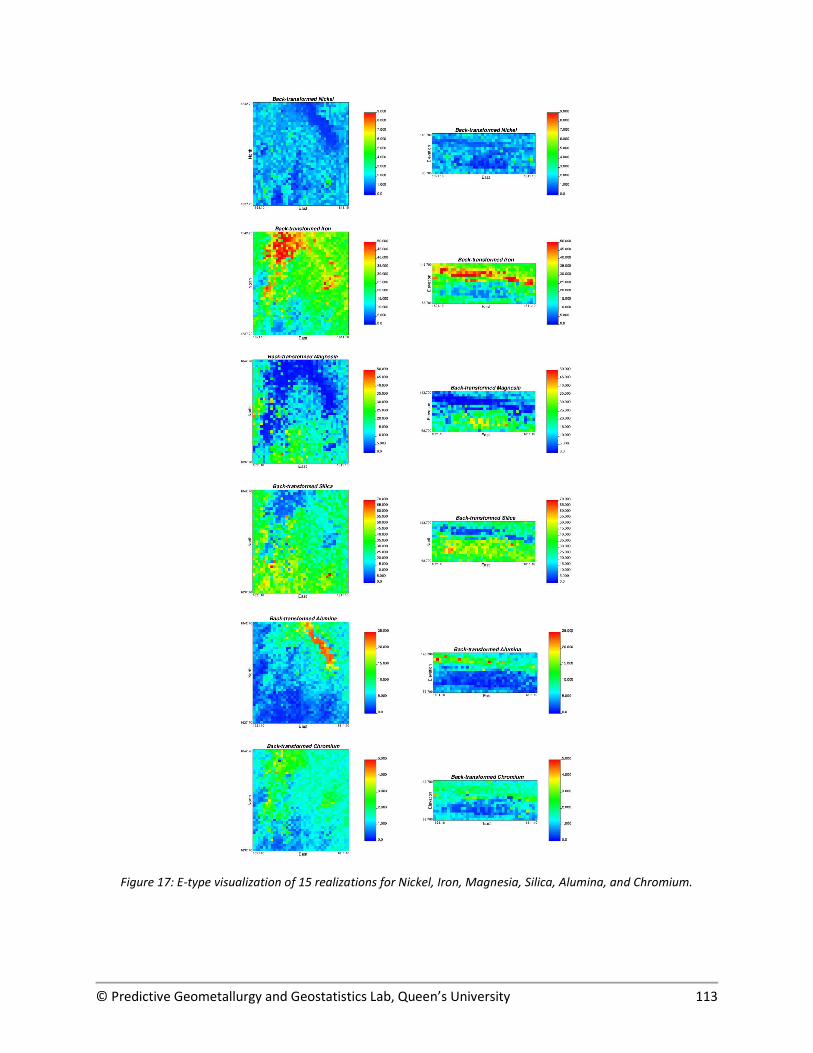
Figure 17: E-type visualization of 15 realizations for Nickel, Iron, Magnesia, Silica, Alumina, and Chromium.


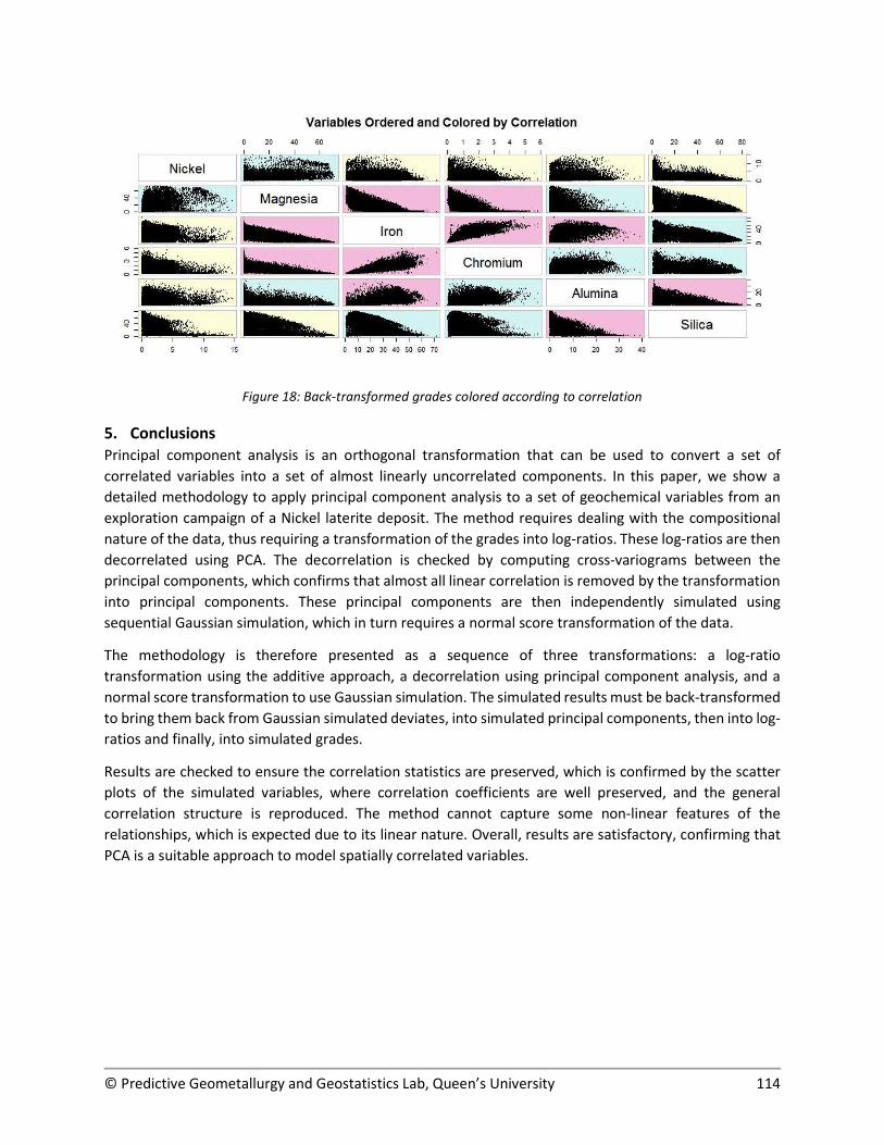
Figure 18: Back-transformed grades colored according to correlation

5. Conclusions Principal component analysis is an orthogonal transformation that can be used to convert a set of correlated variables into a set of almost linearly uncorrelated components. In this paper, we show a detailed methodology to apply principal component analysis to a set of geochemical variables from an exploration campaign of a Nickel laterite deposit. The method requires dealing with the compositional nature of the data, thus requiring a transformation of the grades into log-ratios. These log-ratios are then decorrelated using PCA. The decorrelation is checked by computing cross-variograms between the principal components, which confirms that almost all linear correlation is removed by the transformation into principal components. These principal components are then independently simulated using sequential Gaussian simulation, which in turn requires a normal score transformation of the data.

The methodology is therefore presented as a sequence of three transformations: a log-ratio transformation using the additive approach, a decorrelation using principal component analysis, and a normal score transformation to use Gaussian simulation. The simulated results must be back-transformed to bring them back from Gaussian simulated deviates, into simulated principal components, then into log-ratios and finally, into simulated grades.

Results are checked to ensure the correlation statistics are preserved, which is confirmed by the scatter plots of the simulated variables, where correlation coefficients are well preserved, and the general correlation structure is reproduced. The method cannot capture some non-linear features of the relationships, which is expected due to its linear nature. Overall, results are satisfactory, confirming that PCA is a suitable approach to model spatially correlated variables.


Figure 19: Original Grades

Figure 20: Back-transformed grades after Principal Component Analysis

Figure 21: Back-transformed grades after Co-simulation


Principal Component Analysis reproduces decorrelated factors. The simulation of the PCs and the back-transformation to the original grades achieves better reproduction of the relationship between the variables comparing to the co-simulation, although care has to be taken to ensure a good reproduction of the global statistical distributions. Transformations need to be thoroughly tested to ensure histograms are reproduced at every step.

The approach was compared with cosimulation. Cosimulation is difficult to implement because the LMC constrains the modeling of direct and cross variograms. As a result, cosimulation performance is deteriorated, which is reflected in poor reproduction of the multivariate distribution (reflected in the bivariate scatter plots). PCA tends to better reproduce the bivariate relationships.

6. Acknowledgments We acknowledge the support of the Natural Sciences and Engineering Research Council of Canada (NSERC), funding reference number RGPIN-2017-04200 and RGPAS-2017-507956.

7. References Aitchison, J. (1982) The statistical analysis of compositional data (with discussion). Journal of the Royal

Statistical Society, Series B (Statistical Methodology) 44 (2): 139-177.

Aitchison, J. (1986) The statistical analysis of compositional data. Monographs on Statistics and Applied Probability, London, Chapman & Hall Ltd., 416 p.

Almeida, A.S., Journel, A.G. (1994) Joint simulation of multiple variables with a Markov-type coregionalization model. Mathematical Geology 26(5): 565-588.

Chiles, J-P, Delfiner, P. (2012) Geostatistics – Modeling Spatial Uncertainty, Second Edition. Willey, 699 p.

Davis, B.M., Greenes, K.A. (1983) Estimating using spatially distributed multivariate data: An example with coal quality. Mathematical Geology, 15(2): 287-300. https://doi.org/10.1007/BF01036071

Davis, J.C. (1986) Statistics and Data Analysis in Geology, 2nd Edition, John Wiley & Sons, New York, 646 p.

Desbarats, A.J., Dimitrakopoulos, R. (2000) Geostatistical simulation of regionalized pore-size distributions using min/max autocorrelation factors. Mathematical Geology 32(8): 919–942.

Deutsch, C.V., Journel, A.G. (1998) GSLIB: Geostatistical Software Library and User’s Guide, Oxford University Press, New York, 2nd edition.

Egozcue, J.J., Pawlowsky-Glahn, V., Mateu-Figueras, G. Barcelo-Vidal C (2003) Isometric Logratio Transformations for Compositional Data Analysis, Mathematical Geology 35 (3): 279-300 https://doi.org/10.1023/A:1023818214614

Goovaerts, P. (1997) Geostatistics for natural resources evaluation. New York, N.Y.: Oxford University Press.

Goulard, M., Voltz, M. (1992). Linear coregionalization model: Tools for estimation and choice of cross-variogram matrix. Mathematical Geology, 24(3), pp.269-286.


Hotelling, H. (1933) Analysis of a complex of statistical variables into principal components. Journal of Educational Psychology, 24: 417-441, 498-520.

Howarth, R.J. (2017) Dictionary of Mathematical Geosciences – With Historical Notes, Springer, 893 pages. DOI 10.1007/978-3-319-57315-1.

Johnson, R. A., Wichern, D. W. (1982) Applied multivariate statistical analysis. Englewood Cliffs, NJ, Prentice-Hall.

Leuangthong, O., Deutsch, C.V. (2003) Stepwise conditional transformation for simulation of multiple variables, Mathematical Geology 35(2):155–173.

Manchuk, J., Deutsch, C.V. (2012). A flexible sequential Gaussian simulation program: USGSIM. Computers & Geosciences, 41, pp.208-216.

Mueller, U.A., Ferreira, J. (2012) The U-WEDGE transformation method for multivariate geostatistical simulation, Mathematical Geosciences 44(4): 427-448.

Pawlowsky-Glahn, V., Egozcue, J. (2006) Compositional data and their analysis: an introduction. Geological Society, London, Special Publications, pp.Geological Society, London, Special Publications 2006, v.264; p1-10.

Pawlowsky-Glahn, V., Olea, R.A. (2004) Geostatistical Analysis of Compositional Data, Oxford University Press, 181 p.

Pyrcz, M., Deutsch, C.V. (2003) Declustering and debiasing, downloaded from http://www.gaa.org.au/pdf/DeclusterDebias-CCG.pdf (February, 2019).

Silva, D.S.F., Deutsch, C.V. (2016). Multivariate data imputation using Gaussian mixture models.Spatial Statistics 27: 74-90.

Suro-Perez, V., Journel, A.G. (1991) Indicator Principal Component Kriging, Mathematical Geology, 23(5): 759-788. https://doi.org/10.1007/BF02082535

Verly, G. (1993) Sequential Gaussian co-simulation: a simulation method integrating several types of information, Geostatistics Troia ’92, A. Soares (ed.), volume 1, 543-554, Kluwer Academic Publishers, Dordrecht.

Wackernagel, H. (2003) Multivariate geostatistics. Third Edition. Berlin, Springer. 387 p.

Webster, R., Oliver, M.A. (1990) Statistical methods in soil and land resource survey, Oxford University Press, New York, 316 p.

Multivariate Geostatistical Simulation using Principal ...

Documents