Multivariate characterization of differences between ...eric.univ-lyon2.fr/~ricco/cours/slides/en/analyse_discriminante... · Ricco Rakotomalala Tutoriels Tanagra - 1 Ricco RAKOTOMALALA

Ricco Rakotomalala

Tutoriels Tanagra - http://tutoriels-data-mining.blogspot.fr/ 1

Ricco RAKOTOMALALA

Multivariate characterization of differences between groups

http://tutoriels-data-mining.blogspot.fr/





Ricco Rakotomalala


Outline

1. Problem statement

2. Determination of the latent variables (dimensions)

3. Reading the results

4. A case study

5. Classification of a new instance

6. Statistical tools (Tanagra, lda of R, proc candisc of SAS)

7. Conclusion

8. References






Ricco Rakotomalala







Ricco Rakotomalala


Descriptive Discriminant Analysis (DDA) - Goal

A population is subdivided in K groups (using a categorical variable, a label);

the instances are described by J continuous descriptors.

E.g. Bordeaux wine (Tenenhaus,

2006; page 353). The rows of the

dataset correspond to the year of

production (1924 to 1957)

Goal(s) :

(1) Descriptive (explanation): highlighting the characteristics which enable to

explain the differences between groups main objective in our context

(2) Predictive (classification): assign a group to an unseen instance secondary

objective in our context (but this is the main objective in the predictive

discriminant analysis [PDA] context)

Descriptors Group membership

Annee Temperature Soleil Chaleur Pluie Qualite

1924 3064 1201 10 361 medium

1925 3000 1053 11 338 bad

1926 3155 1133 19 393 medium

1927 3085 970 4 467 bad

1928 3245 1258 36 294 good

1929 3267 1386 35 225 good

Sun Heat Rain Quality






Ricco Rakotomalala


Descriptive Discriminant Analysis - Approach

Aim: Determining the most parsimonious way to explain the differences between groups

by computing a set of orthogonal linear combinations (canonical variables, factors) from

the original descriptors. Canonical Discriminant Analysis.

850

950

1050

1150

1250

1350

1450

1550

1650

1750

2800 3000 3200 3400 3600 3800

Sole

il

Temperature

1er axe AFD sur les var. Temp et Soleil

bad

good

medium

)()( 222111 xxaxxaz iii The conditional centroids must be as widely

separated as possible on the factors.

i k k i

kikkki zzzznzz222

v = b + w Total (variation) = Between class (variation) + Within class (variation)






Ricco Rakotomalala


Descriptive Discriminant Analysis – Approach (continued)

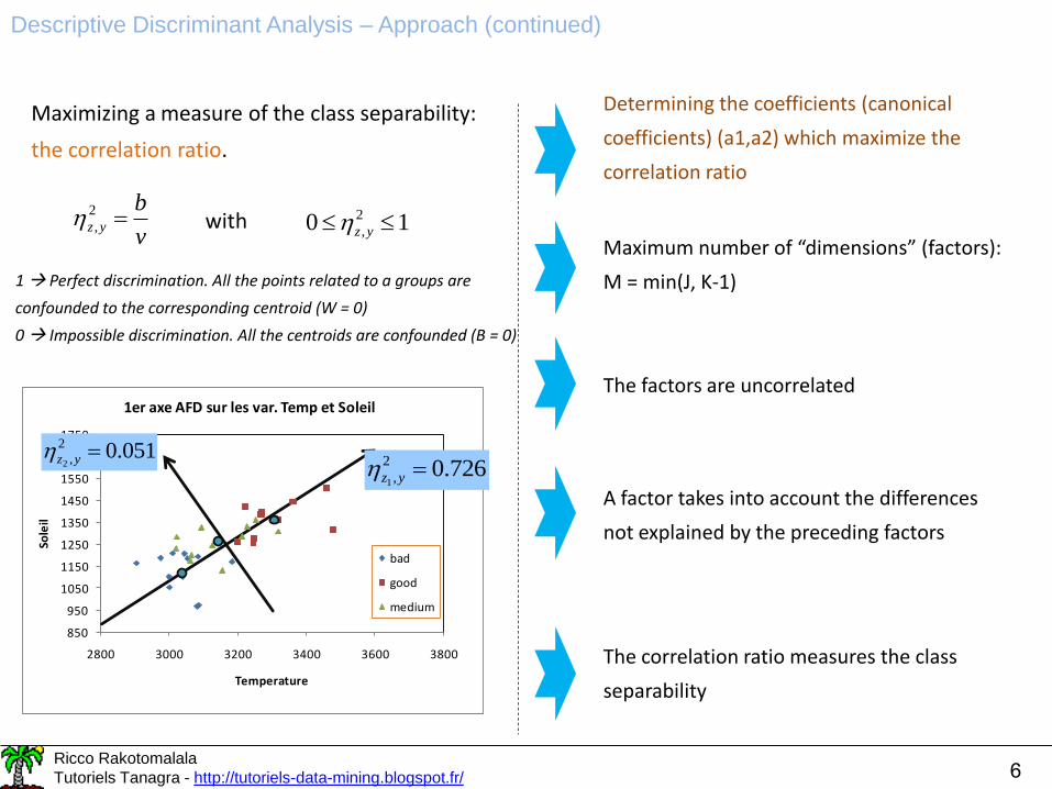
v

byz 2

, 10 2

, yzwith

1 Perfect discrimination. All the points related to a groups are

confounded to the corresponding centroid (W = 0)

0 Impossible discrimination. All the centroids are confounded (B = 0)

Maximizing a measure of the class separability:

the correlation ratio.

Determining the coefficients (canonical

coefficients) (a1,a2) which maximize the

correlation ratio

Maximum number of “dimensions” (factors):

M = min(J, K-1)

The factors are uncorrelated

The correlation ratio measures the class

separability

850

950

1050

1150

1250

1350

1450

1550

1650

1750

2800 3000 3200 3400 3600 3800

Sole

il

Temperature

1er axe AFD sur les var. Temp et Soleil

bad

good

medium

726.02

,1yz

051.02

,2yz

A factor takes into account the differences

not explained by the preceding factors






Ricco Rakotomalala







Ricco Rakotomalala


Descriptive Discriminant Analysis

Mathematical formulation

Total covariance matrix

i

ciclillc xxxxn

vV1

Ja

a

a 1

« a » is the vector of coefficients

which enables to define the

canonical variable Z i.e.

VaaTSS '

Within groups covariance matrix

k kyi

kckicklkillc

i

xxxxn

wW:

,,,,

1

Between groups covariance matrix

WaaRSS '

k

ckclklk

lc xxxxn

nbB ,,

BaaESS '

Huyghens’ theorem V = B + W

The aim of DDA is to calculate the coefficients of the canonical

variable which maximizes the correlation ratio

2

,max'

'max yz

aa Vaa

Baa

)()( 111 JJJ xxaxxaz

[ignoring a multiplication

factor (1/n)]

Total sum of squares






Ricco Rakotomalala


Vaa

Baa

a '

'max is equivalent to

Baaa

'max

Under the constraint 1' Vaa (“a” is a unit vector)

Solution: using the Lagrange function ( is the Lagrange multiplier)

1'')( VaaBaaaL

aBaV

VaBaa

aL

1

0)(

is the first eigenvalue of V-1B

“a” is the corresponding eigenvector

The successive canonical variables are obtained from the eigenvalues and the eigenvectors of V-1B.

2 The eigenvalue is equal to the square of the correlation ratio (0 ≤ ≤ 1)

is the canonical correlation

The number of non-zero eigenvalue is M = min(K-1, J) i.e. M canonical variables

Descriptive Discriminant Analysis

Solution






Ricco Rakotomalala


Discriminant descriptive analysis

Bordeaux wine (X1 : Temperature and X2 : Sun)

852.0726.0

0075.00075.0

1

22111

xxxxZ iii

225.0051.0

0105.00092.0

2

22112

xxxxZ iii

The differences between the centroids

are high on this factor.

The differences between the centroids are

lesser on this factor.

Number of factors

M = min (J = 2; K-1 = 2) = 2

-2.5

-2.0

-1.5

-1.0

-0.5

0.0

0.5

1.0

1.5

2.0

-4.0 -3.0 -2.0 -1.0 0.0 1.0 2.0 3.0 4.0 5.0

bad

good

medium

good

medium

bad

(2.91; -2.22): the coordinates of the

individuals in the new representation

space are called “factor scores” (SAS,

SPSS, R…)






Ricco Rakotomalala


Discriminant descriptive analysis

Alternative solution – English-speaking tools and references

Waa

Baa

a '

'max

is equivalent

to

Baaa

'max

w.r.t. 1' Waa

Since V = B + W, we can formulate the problem in other way:

The factors are obtained from the eigenvalues and eigenvector of W-1B.

The eigenvectors of W-1B are the same as those of V-1B the factors are identical.

The eigenvalues are related with the following formula:

= ESS / RSS m

mm

1

E.g. Bordeaux wine

With only the variables “temperature” and “sun”

Root Eigenvalue Proportion Canonical R

1 2.6432 0.9802 0.8518

2 0.0534 1 0.2251

7255.01

7255.0

8518.01

8518.06432.2

2

2

we can state also the explained variation in

percentage

E.g. The first factor explains 98% of the global between-class variation: 98%

= 2.6432 / (2.6432 + 0.0534).

The two factors explain 100% of this variation [M = min(2, 3-1) = 2]

The first factor is enough here!

(“a” is a unit vector)






Ricco Rakotomalala







Ricco Rakotomalala


Descriptive Discriminant Analysis – Determining the right number of factors

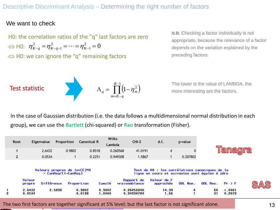
In the case of Gaussian distribution (i.e. the data follows a multidimensional normal distribution in each

group), we can use the Bartlett (chi-squared) or Rao transformation (Fisher).

H0: the correlation ratios of the "q" last factors are zero

H0:

H0: we can ignore the “q” remaining factors

02

1

2

1

2 KqKqK

We want to check

N.B. Checking a factor individually is not

appropriate, because the relevance of a factor

depends on the variation explained by the

preceding factors.

Test statistic

1

21K

qKm

mq The lower is the value of LAMBDA, the

more interesting are the factors.

Root Eigenvalue Proportion Canonical RWilks

LambdaCHI-2 d.f. p-value

1 2.6432 0.9802 0.8518 0.260568 41.0191 4 0

2 0.0534 1 0.2251 0.949308 1.5867 1 0.207802

The two first factors are together significant at 5% level; but the last factor is not significant alone.






Ricco Rakotomalala


H0: all the correlation ratio are zero

H0:

H0: we cannot distinguish the groups

centroid in the global representation space

02

1

2

1 K

MANOVA test i.e. comparing multivariate

means (centroids) of several groups

KJ

K

J

H

,

,1

1,

1,1

0 :

simultaneously

1

1

21K

m

mTest statistic:

Wilks’ LAMBDA

The lower is the value of LAMBDA, the more

different are the centroids (0 ≤ ≤ 1).

950

1050

1150

1250

1350

1450

1550

2800 3000 3200 3400 3600

Sole

il

Temperature

Moyennes conditionnelles

Temperature vs. Soleil

bad

good

medium

LAMBDA de Wilks = 0.26

Bartlett transformation

CHI-2 = 41.02 ; p-value < 0.0001

Rao transformation

F = 14.39 ; p-value < 0.0001

Conclusion: At least

one centroid is

different to the others.

Descriptive Discriminant Analysis – Checking all the factors






Ricco Rakotomalala


Descriptive discriminant analysis – Interpreting the canonical variables (factors)

Standardized and unstandardized canonical coefficients

JJ

JJJ

xaxaa

xxaxxaZ

110

111 )()(

Unstandardized coefficients

These coefficients enables to calculate the

canonical scores of the individuals (coordinates

of the individuals, discriminant scores) The unstandardized canonical coefficients do not allow to compare the

influence of the variables because they are not defined on the same unit.

Standardized coefficients

These are the coefficients of the DDA on standardized

variables. We can obtain the same values by

multiplying the unstandardized coefficients with the

pooled within-class standard deviation of the

variables. The coefficients (influence) of the variables

become comparable.

jjj a

k

n

kyi

kjkijj

k

i

xxKn :

2

,,

2 1

The pooled within class variance of

the variable Xj

Standardized coefficients show the variable's contribution to calculating the discriminant score. Two

correlated variables share their contribution, their true influence may be hidden (W.R. Klecka, “Discriminant

Analysis”, 1980 ; page 33).

We must complete this analysis by studying the structure coefficients table.

Quality = DDA (Temperature, Sun) >>

Canonical Discriminant FunctionCoefficients

Attribute Root n°1 Root n°2 Root n°1 Root n°2

Temperature 0.007465 -0.009214 -0.653736 -0.806832

Sun 0.007479 0.010459 -0.604002 0.844707

constant 32.903185 16.049255

Unstandardized Standardized

-






Ricco Rakotomalala


These are the bivariate correlation between the variables and the canonical variables.

We can visualize the correlation circle such as for PCA (principal component analysis).

Correlation scatterplot (CDA_1_Axis_1 vs. CDA_1_Axis_2)

CDA_1_Axis_1

10.90.80.70.60.50.40.30.20.10-0.1-0.2-0.3-0.4-0.5-0.6-0.7-0.8-0.9-1

CD

A_1_A

xis

_2

1

0.9

0.8

0.7

0.6

0.5

0.4

0.3

0.2

0.1

0

-0.1

-0.2

-0.3

-0.4

-0.5

-0.6

-0.7

-0.8

-0.9

-1

Soleil

Temperature

-2.5

-2.0

-1.5

-1.0

-0.5

0.0

0.5

1.0

1.5

2.0

-4.0 -3.0 -2.0 -1.0 0.0 1.0 2.0 3.0 4.0 5.0

bad

good

medium

The 1st factor corresponds to the combination of high

temperature and high periods of sunshine.

The combination of high temperature and high

periods of sunshine correspond to "good" wine.

These correlation coefficients allow to interpret easily the factors.

If the sign are different to the standardized canonical coefficients collinearity between the variables.

Descriptors Total

Temperature 0.9334

Sun 0.9168


Total structure coefficients






Ricco Rakotomalala


2 800

2 900

3 000

3 100

3 200

3 300

3 400

3 500

3 600

-4.00 -2.00 0.00 2.00 4.00 6.00

Tem

pé

ratu

re

Axe 1

bad

good

medium

-150

-100

-50

0

50

100

150

200

Tem

pé

ratu

re

Axe 1

bad

good

medium

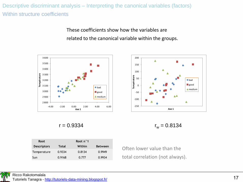
These coefficients show how the variables are

related to the canonical variable within the groups.

r = 0.9334 rw = 0.8134

Often lower value than the

total correlation (not always).

Root

Descriptors Total Within Between

Temperature 0.9334 0.8134 0.9949

Sun 0.9168 0.777 0.9934

Root n°1


Within structure coefficients






Ricco Rakotomalala


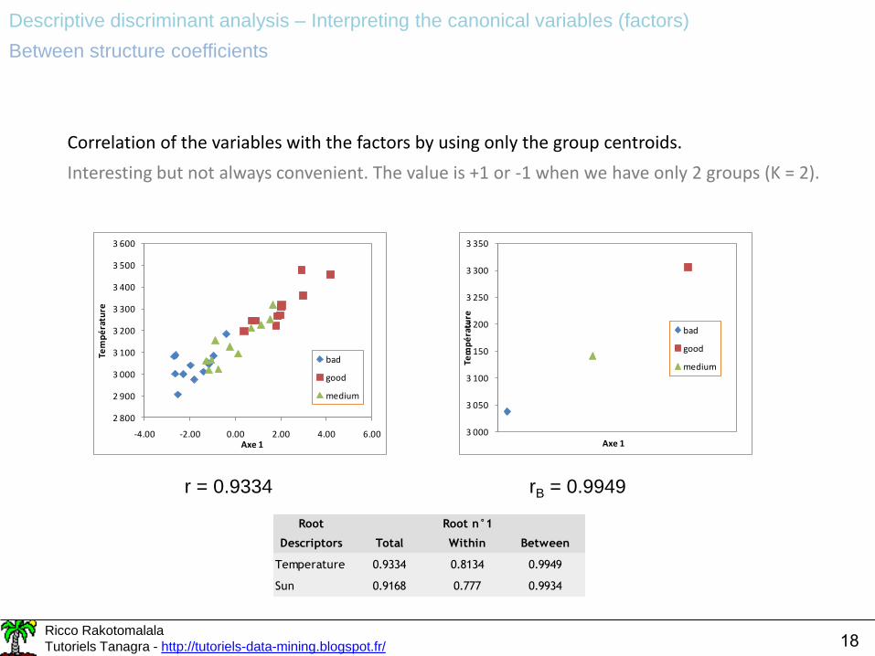
Correlation of the variables with the factors by using only the group centroids.

Interesting but not always convenient. The value is +1 or -1 when we have only 2 groups (K = 2).

2 800

2 900

3 000

3 100

3 200

3 300

3 400

3 500

3 600

-4.00 -2.00 0.00 2.00 4.00 6.00

Tem

pé

ratu

re

Axe 1

bad

good

medium

3 000

3 050

3 100

3 150

3 200

3 250

3 300

3 350

Tem

pé

ratu

re

Axe 1

bad

good

medium

r = 0.9334 rB = 0.9949

Root

Descriptors Total Within Between

Temperature 0.9334 0.8134 0.9949

Sun 0.9168 0.777 0.9934

Root n°1


Between structure coefficients






Ricco Rakotomalala


Calculating the coordinates of the centroids in the new representation space.

This allows to identify the groups which are well highlighted.

(X1) CDA_1_Axis_1 vs. (X2) CDA_1_Axis_2 by (Y) TYPE

KIRSCH POIRE MIRAB

43210-1-2-3

3

2

1

0

-1

-2

TYPE Root n°1 Root n°2

KIRSCH 3.440412 0.031891

POIRE -1.115293 0.633275

MIRAB -0.981677 -0.674906

Sq Canonical corr. 0.789898 0.2544

(X1) CDA_1_Axis_1 vs. (X2) CDA_1_Axis_2 by (Y) Qualite

medium bad good

210-1-2-3-4

1

0

-1

-2

Qualite Root n°1 Root n°2

bad -1.804187 0.153917

good 1.978348 0.151489

medium -0.01015 -0.3194


The three groups are quite separate on the first factor

Nothing interesting on the second factor (low canonical correlation)

KIRSCH vs. the two other groups on the 1st factor

POIRE vs. MIRAB on the 2nd factor (significant canonical correlation)


Group centroids into the discriminant representation space






Ricco Rakotomalala







Ricco Rakotomalala


Bordeaux wine - Description of the dataset

Temperature

1000 1200 1400 300 500

2900

3100

3300

3500

1000

1200

1400

Sun

Heat

10

20

30

40

2900 3100 3300 3500

300

500

10 20 30 40

Rain

Some of the descriptors are correlated

(see the correlation matrix)

(Red : Bad ; blue : Medium ; green : Good).

The groups are discernible, especially for

some combination of variables.

The influence on the quality is not the

same according to the variables.

There are outliers...

Correlation matrix






Ricco Rakotomalala


Bordeaux wine – Univariate analysis of the variables

Conditional distribution and correlation ratio

bad good medium

2900

3100

3300

3500

Temperature

bad good medium

1000

1200

1400

Sun

bad good medium

10

20

30

40

Heat

bad good medium

300

400

500

600

Rain

64.02

, yx 62.02

, yx

50.02

, yx 35.02

, yx

“Temperature”, “Sun” and “Heat”

enable to well distinguish the

groups. "Rain" seems less decisive.

For all the variables, the univariate

one-way ANOVA (the class means

are equal or not) is significant at

5% level.






Ricco Rakotomalala


Bordeaux wine – DDA results


medium bad good

3210-1-2-3-4

1

0

-1

-2

Roots and Wilks' Lambda

Root Eigenvalue Proportion Canonical RWilks

LambdaCHI-2 d.f. p-value

1 3.27886 0.95945 0.875382 0.205263 46.7122 8 0

2 0.13857 1 0.348867 0.878292 3.8284 3 0.280599

Group centroids on the canonical variables

Qualite Root n°1 Root n°2

medium -0.146463 0.513651

bad 2.081465 -0.22142

good -2.124227 -0.272102


On the first factor, we observe the 3 groups. From

the left to the right, we have the centroids of

“good”, “medium” and “bad”.

The square of the correlation ratio for this factor is

0.766. This is higher than any univariate correlation

ratio of the variables (the higher is "temperature"

with ² = 0.64).

(a) The difference between

groups is significant. (b) 96% of

between-class variation is

explained by the first factor. (c)

The 2nd factor is not significant

at 5% level, we can ignore it.






Ricco Rakotomalala



medium bad good

3210-1-2-3-4

1

0

-1

-2

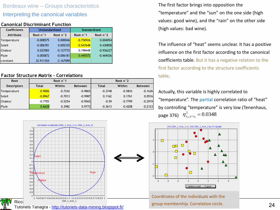
Canonical Discriminant FunctionCoefficients

Attribute Root n°1 Root n°2 Root n°1 Root n°2

Temperature -0.008575 0.000046 -0.750926 0.004054

Soleil -0.006781 0.005335 -0.547648 0.430858

Chaleur 0.027083 -0.127772 0.198448 -0.936227

Pluie 0.005872 -0.006181 0.445572 -0.469036

constant 32.911354 -2.167589

Factor Structure Matrix - CorrelationsRoot

Descriptors Total Within Between Total Within Between

Temperature -0.9006 -0.7242 -0.9865 -0.3748 -0.5843 -0.1636

Soleil -0.8967 -0.7013 -0.9987 0.1162 0.1761 0.0516

Chaleur -0.7705 -0.5254 -0.9565 -0.59 -0.7799 -0.2919

Pluie 0.6628 0.3982 0.9772 -0.3613 -0.4208 -0.2123

Unstandardized Standardized

-

Root n°1 Root n°2

The first factor brings into opposition the

“temperature” and the “sun” on the one side (high

values: good wine), and the “rain” on the other side

(high values: bad wine).

The influence of “heat” seems unclear. It has a positive

influence on the first factor according to the canonical

coefficients table. But it has a negative relation to the

first factor according to the structure coefficients

table.

Actually, this variable is highly correlated to

“temperature”. The partial correlation ratio of “heat”

by controlling “temperature” is very low (Tenenhaus,

page 376) 0348.02

/, 13xyx


CDA_1_Axis_1

10.90.80.70.60.50.40.30.20.10-0.1-0.2-0.3-0.4-0.5-0.6-0.7-0.8-0.9-1

CD

A_1_A

xis

_2

1

0.9

0.8

0.7

0.6

0.5

0.4

0.3

0.2

0.1

0

-0.1

-0.2

-0.3

-0.4

-0.5

-0.6

-0.7

-0.8

-0.9

-1

Temperature

Soleil

Chaleur

Pluie

Coordinates of the individuals with the

group membership. Correlation circle.

Bordeaux wine – Groups characteristics

Interpreting the canonical variables






Ricco Rakotomalala







Ricco Rakotomalala


Classification rule

Preamble

The linear (predictive) discriminant analysis (PDA) offers a more attractive theoretical framework

for prediction, with explicit probabilistic assumptions.

Nevertheless, we can use the results of the DDA to classify individuals based on geometric rules.

-2.5

-2.0

-1.5

-1.0

-0.5

0.0

0.5

1.0

1.5

2.0

2.5

-2.5 -2.0 -1.5 -1.0 -0.5 0.0 0.5 1.0 1.5 2.0 2.5

AFD sur Température et SoleilBarycentres conditionnels

bad

good

mediumWhich group?

Steps:

1. As from the description of the individual,

its coordinates in the discriminant

dimensions are computed.

2. The distance to the conditional centroids

is computed.

3. The instance is assigned to the group of

which the centroid is the closest.






Ricco Rakotomalala


DDA from Temperature (X1) and Sun (X2)

X1 = 3000 – X2 = 1100 – Year 1958 (based on the weather forecast )

0862.0

032152.161100010448.03000009204.0

032152.16010448.0009204.0

2780.2

868122.321100007471.03000007457.0

868122.32007471.0007457.0

212

211

xxz

xxz

1. Calculating the coordinates

2. Calculating the distance to the centroids

3075.5)(

1031.18)(

2309.0

))1538.0(0832.0())8023.1(2780.2()(

2

2

222

mediumd

goodd

badd

3. Conclusion

The vintage 1958 has a high probability to

be “bad”. It has a very low probability to be

“good”.

-2.5

-2.0

-1.5

-1.0

-0.5

0.0

0.5

1.0

1.5

2.0

2.5

-2.5 -2.0 -1.5 -1.0 -0.5 0.0 0.5 1.0 1.5 2.0 2.5

AFD sur Température et SoleilBarycentres conditionnels

bad

good

medium

0.2309 18.1031

5.3075






Ricco Rakotomalala


Classifying an new instance

Euclidian distance into the discriminant dimensions = Mahalanobis distance into the initial representation space

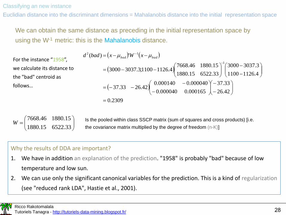
We can obtain the same distance as preceding in the initial representation space by

using the W-1 metric: this is the Mahalanobis distance.

2309.0

42.26

33.37

000165.0000040.0

000040.0000140.042.2633.37

4.11261100

3.30373000

33.652215.1880

15.188046.76684.11261100;3.30373000

')(

1

12

badbad xWxbadd

33.652215.1880

15.188046.7668W

For the instance “1958”,

we calculate its distance to

the "bad" centroid as

follows…

Is the pooled within class SSCP matrix (sum of squares and cross products) [i.e.

the covariance matrix multiplied by the degree of freedom (n-K)]

Why the results of DDA are important?

1. We have in addition an explanation of the prediction. "1958" is probably "bad" because of low

temperature and low sun.

2. We can use only the significant canonical variables for the prediction. This is a kind of regularization

(see "reduced rank LDA", Hastie et al., 2001).






Ricco Rakotomalala


Q

m

kmimkmim

Q

m

kmimi

zzzz

zzkd

1

,

2

,

2

1

2

,

2

2

)(

For an instance “i”, we calculate as follows its distance

to the centroid of the group “k”. We take into account Q

canonical variables (Q = M if we treat all the factors). k

iik

kfkkdk )(maxarg*)(minarg* 2

Q

m

km

Q

m

imkm

Q

m

kmimkmi

zzz

zzzkf

1

2

,

1

,

1

2

,,

2

1

2

1)(

Finding the closest centroid (minimization). We

can transform it in a maximization problem by

multiplying with -0.5

JJmmmmm xaxaxaaz 22110

Discriminant function

for the factor “m”

We have a linear classification function.

E.g. Bordeaux wine with “temperature” (x1)

and “sun” (x2) – Only one factor (Q = 1)

3331.00001.00001.0)(

9081.660148.00147.0)(

6129.570135.00134.0

8023.12

1868122.32007471.0007457.08023.1)(

21

21

21

2

21

xxmediumf

xxgoodf

xx

xxbadf

For the instance (x1 = 3000; x2 = 1100) 0230.0)(

5447.6)(

4815.2)(

mediumf

goodf

badfConclusion: the vintage “1958” will

be probably « bad »


Specifying an explicit model






Ricco Rakotomalala


The parametric linear discriminant analysis makes assumptions about the distribution

and the dispersion of the observations (normal distribution, homogeneity of

variances/covariances)

'2

1'ln),( 11

kkkkk XyYPXYd Classification

function from PDA

Classification rule from the DDA when

we handle all the factors (M factors)

Equivalence

In conclusion, the classification rule of DDA is equivalent to

the one of PDA if we have balanced class distribution i.e.

KyYPyYP K

11

Some tools make this assumption by default (e.g. default settings for the SAS PROC DISCRIM)

Introducing the correction derived from the estimated class distribution will improve the

error rate (Hastie et al., 2001 ; page 95).


What is the connection with the linear (predictive) discriminant analysis (PDA)?






Ricco Rakotomalala







Ricco Rakotomalala


DDA with TANAGRA

CANONICAL DISCRIMINANT ANALYSIS tool

The main results, usable for the interpretation, are

available.

We can obtain the graphical representation of the

individuals and the correlation circle for the variables

(based on the total structure correlation).

French references use (1/n) for the estimation of the

covariance.






Ricco Rakotomalala


DDA with TANAGRA

Graphical representation


CDA_1_Axis_1

10.90.80.70.60.50.40.30.20.10-0.1-0.2-0.3-0.4-0.5-0.6-0.7-0.8-0.9-1

CD

A_1_A

xis

_2

1

0.9

0.8

0.7

0.6

0.5

0.4

0.3

0.2

0.1

0

-0.1

-0.2

-0.3

-0.4

-0.5

-0.6

-0.7

-0.8

-0.9

-1

Temperature

Sun

Heat

Rain

(X1) CDA_1_Axis_1 vs. (X2) CDA_1_Axis_2 by (Y) Quality

medium bad good

3210-1-2-3-4

1

0

-1

-2

Plotting the individuals into the

discriminant dimensions

Correlation circle






Ricco Rakotomalala


-4 -2 0 2

-3-2

-10

12

3

LD1

LD

2

medium

bad

medium

bad

good

good

bad

bad

bad

medium

good

bad

badgood

medium

medium

medium

bad

medium

good

mediumgood

medium

good

medium

good

medium bad

good

good

bad

good

bad

bad

DDA with R

The “lda” procedure from the MASS package

The output is concise.

But with some programming instructions,

we can obtain better. This is one of the

main advantages of R.

English-speaking references use [1/(n-1)]

for the estimation of the covariance.






Ricco Rakotomalala


DDA with R

-4 -2 0 2 4

-3-2

-10

12

3

Carte factorielle

Axe.1

Axe

.2

badgood

mediumWith some programming instructions,

the result is worth it …






Ricco Rakotomalala


DDA with SAS

The CANDISC procedure

Comprehensive results.

The “ALL” option allows to

obtain all the intermediate

results (matrices V, W, B ; etc.).

English-speaking references use

[1/(n-1)] for the estimation of the

covariance (such as R).






Ricco Rakotomalala







Ricco Rakotomalala


Conclusion

DDA: multivariate method for groups’ description and characterization

Tools for the interpretation of the results (test for significance of canonical variables,

canonical coefficients, structure coefficients...)

Tools for the visualization of the results (individuals, variables)

The approach is related to other factorial methods (principal component analysis,

canonical correlation)

The approach is in nature descriptive, but it can be implemented in a predictive

framework easily.

The approach provides a white-box prediction (we can understand for which reason

an unseen instance is assigned to such group).






Ricco Rakotomalala


References

M. Tenenhaus, “Statistique – Méthodes pour décrire, expliquer et prévoir” (Statistics - Methods

to describe, explain and predict), Dunod, 2007. Chapter 10, pages 351 to 386.

W.R. Klecka, “Discriminant Analysis”, Sage University Paper series on Quantitative

Applications in the Social Sciences, n°07-019, 1980.

C.J. Huberty, S. Olejnik, “Aplied MANOVA and Dscriminant Analysis”, 2nd Edition, Wiley, 2006.






Multivariate characterization of differences between ...eric.univ-lyon2.fr/~ricco/cours/slides/en/analyse_discriminante... · Ricco Rakotomalala Tutoriels Tanagra - 1 Ricco RAKOTOMALALA

Documents