Multivariate Bayesian Regression Approach to Forecast Releases from a System of Multiple Reservoirs

Water Resour Manage (2011) 25:523–543DOI 10.1007/s11269-010-9712-y

Multivariate Bayesian Regression Approach to ForecastReleases from a System of Multiple Reservoirs

Andres M. Ticlavilca · Mac McKee

Received: 17 January 2010 / Accepted: 14 September 2010 /Published online: 28 September 2010© Springer Science+Business Media B.V. 2010

Abstract This research presents a model that simultaneously forecasts requiredwater releases 1 and 2 days ahead from two reservoirs that are in series. In practice,multiple reservoir system operation is a difficult process that involves many decisionsfor real-time water resources management. The operator of the reservoirs has torelease water from more than one reservoir taking into consideration different waterrequirements (irrigation, environmental issues, hydropower, recreation, etc.) in atimely manner. A model that forecasts the required real-time releases in advancefrom a multiple reservoir system could be an important tool to allow the operatorof the reservoir system to make better-informed decisions for releases neededdownstream. The model is developed in the form of a multivariate relevance vectormachine (MVRVM) that is based on a sparse Bayesian regression model approach.With this Bayesian approach, a predictive confidence interval is obtained from themodel that captures the uncertainty of both the model and the data. The model isapplied to the multiple reservoir system located in the Lower Sevier River Basinnear Delta, Utah. The results show that the model learns the input–output patternswith high accuracy. Computing multiple-time-ahead predictions in real-time wouldrequire a model which guarantees not only good prediction accuracy but also robust-ness with respect to future changes in the nature of the inputs data. A bootstrapanalysis is used to guarantee good generalization ability and robustness of theMVRVM. Test results demonstrate good performance of predictions and statisticsthat indicate robust model generalization abilities. The MVRVM is compared interms of performance and robustness with another multiple output model such asArtificial Neural Network (ANN).

A. M. Ticlavilca (B) · M. McKeeUtah Water Research Laboratory and Department of Civil and Environmental Engineering,Utah State University, 8200 Old Main Hill, Logan, UT 84322-8200, USAe-mail: [email protected]

M. McKeee-mail: [email protected]

524 A.M. Ticlavilca, M. McKee

Keywords Forecasting · Reservoir · Water management · Bayesian ·Machine learning

1 Introduction

The per capita availability of water resource is decreasing worldwide due to popu-lation growth, climate change, rapidly increasing demands (for irrigation, domesticsupply, recreation, etc.), and pollution. In order to achieve greater operationalefficiency in meeting these increasing demands and decreasing relative supplies,water managers must have better information about future conditions of their watersystems. The purpose of this paper is to use a real-time model that can providevaluable information to the operator of a multiple reservoir system in the form ofmulti-time-ahead release predictions with predictive confidence intervals.

Techniques based on physical modeling have been developed to characterize cur-rent and future states of water resources systems. However, the lack of required dataand the expense of data acquisition can limit the practical applications of physicalbased models (Khalil et al. 2005a). To overcome these limitations, researchers haveused data-driven modeling as an alternative, or a complement, to physically basedmodels (Lobbrecht and Solomatine 2002; Khalil et al. 2005a). Examples of suchmodels include artificial neural network (ANNs), support vector machines (SVMs),and relevance vector machines (RVMs). These types of models are derived from theemerging area of machine-learning theory. They are characterized by their abilityto capture the underlying physics of the system simply by examination of the inputsand outputs of the system. They can be used to provide predictions of the systembehavior using only historical data; they “let the data speak” (Khalil et al. 2005d).

Machine learning models have often been applied in water resources manage-ment. Sivapragasam and Muttil (2005) used SVMs in the extrapolation of stage-discharge rating curves. Their results showed that a SVM model was better suited forextrapolation than a comparable ANN. El-Shafie et al. (2007) proposed an adaptiveneuro-fuzzy inference system (ANFIS) to forecast the monthly inflow from theNile River to a dam. Their results demonstrated that the ANFIS model was moreaccurate than an ANN model. Nourani et al. (2009) presented a multivariate ANN-wavelet model to predict short- and long-term runoff discharges. Their ANN-waveletconjunction model performed better when compared with an Auto Regressive Inte-grated Moving Average (ARIMA) model. Guldal and Tongal (2010) compared fourmodels to predict lake-level changes in Turkey: Recurrent neural network (RNN),ANFIS, auto regressive (AR) and auto-regressive moving average (ARMA). Theirresults indicated that RNN and ANFIS models were more accurate than AR andARMA models.

Dams and reservoir systems have been built to regulate storage and manage waterdistribution. However, many of theses systems are not producing benefits that wouldeconomically justify their development (World Commission on Dams 2000; Labadie2004). As a result, we must focus on improving the operational effectiveness ofexisting reservoir systems to maximize their value (Labadie 2004). Providing a modelthat forecasts releases from a system of multiple reservoirs could be an importanttool in integrated reservoir operation and management. Information on predicted

Multivariate Bayesian Regression Approach to Forecast Multi-Reservoir Releases 525

releases can allow the operator of the multiple reservoir system to make better-informed decisions for releases needed downstream.

The multiple reservoir system operation depends on physical behavior of thewatershed (hydrologic, climatic, environmental, etc.) and human behavior. Humanbehavior takes the form of the reservoir operator who has to release water frommore than one reservoir to fulfill different water requirements. The combinationof all these behaviors may cause unexpected future changes in the reservoir systemoperation which could be extremely difficult to predict. Therefore, it is necessary todevelop predictive models which have the ability to guarantee robustness towardsfutures changes in the system behavior.

Khalil et al. (2005a) applied RVM, which is based on Bayesian learning theory,to predict the real-time operation of a single reservoir. The target output of theirmodel is the hourly prediction of the quantity of water to be released from a singlereservoir in order to meet downstream diversion requirements. Their performanceresults showed that the RVM model was able to predict future system states(generalization ability) and had the capability to estimate the uncertainty of thepredictions (predictive confidence intervals). The research reported here extends thiscapability to a multiple-day-ahead for multi reservoir setting.

In order to obtain multiple-time-ahead predictions with (predictive) confidenceintervals, the model exploits the capability of the Multivariate Relevance VectorMachine (MVRVM) (Thayananthan 2005). The model forecasts the water releasesof two reservoirs simultaneously having as inputs recent historical data on reservoirreleases, diversions into canals, weather, and streamflows. The target outputs are thepredictions of the required water releases from two reservoirs. These predictionsare made 1 and 2 days ahead, simultaneously for each reservoir. Therefore, themodel recognizes the patterns between future reservoir releases and historical datacollected from the system.

The MVRVM is a Bayesian regression tool extension of the RVM algorithmdeveloped by Tipping and Faul (2003) to produce multivariate outputs when given aset of inputs. In addition to its ability to predict multiple outputs, the MVRVM hasthe same properties of the conventional RVM: high prediction accuracy, robustnessand characterization of uncertainty in the predictions. Therefore, developing a modelwith all these properties can work as a practical decision support tool in real-timewater resources management by providing multiple predictions that are difficult (ornot practical) to obtain from traditional modeling approaches.

The remainder of the paper describes the MVRVM learning model, the area ofstudy where the model has been applied, how the model has been developed for amultiple reservoir system, the results of the MVRVM application, the comparisonwith the performance of an ANN model, and conclusions that can be drawn.

2 Model Description

Thayananthan (2005) proposed the Multivariate Relevance Vector Machine(MVRVM) to provide a regression tool capable of generating multivariate outputs.This model is an extension of the sparse Bayesian model developed by Tipping andFaul (2003). It is developed as follows.


Given a training data set of input-target vector pairs {x(n), t(n)}Nn=1, where N is the

number of observations, x ε RD is a D-dimensional input vector, t ε RM is a M-dimensional output target vector; the model has to “learn” the dependency betweeninput and output target with the purpose of making accurate predictions of t forpreviously unseen values of x:

t = W� (x) + ε (1)

where W is a M × Q weight matrix and Q = N + 1. A fixed kernel func-tion K(x, x j) is used to create a vector of basis functions of the form �(x) =[1, K

(x, x(1), . . . K

(x, x(N)

)). The error εεε is conventionally assumed to be zero-mean

Gaussian with diagonal covariance matrix S = diag(σ2

1, ..., σ2M

).

Let t = [τττ1, ...,τττr, ...,τττM]T and W = [w1, ..., wr, ..., wM]T. A likelihood distributionof the weight matrix can be written as a product of Gaussians of the weight vectors(wr) corresponding to each target output (τττr) (Thayananthan et al. 2008):

p({

t(n)}N

n=1

∣∣W, S)

=N∏

n=1

N(t(n)

∣∣W�(x(n)

), S

) =M∏

r=1

N(τ r

∣∣wr�,σ2r

)(2)

where �� = [1, �(x1),�(x2), ..., �(xN)]. Equation 2 contains several parameters. Asa result, there is a danger that the maximum likelihood estimation of wr andσ2

r will suffer from severe over-fitting. To avoid this, Tipping (2001) proposedconstraining the selection of parameters by applying a Bayesian perspective anddefining an explicit zero-mean Gaussian prior probability distribution over theweights (Thayananthan et al. 2008):

p (W|A) =M∏

r=1

Q∏

j=1

N(

wrj|0,α−2j

)=

M∏

r=1

N (wr|0, A) (3)

where A = diag(α−21 , ..., α−2

Q )T is a hyperparameter matrix and wrj is the (r,j)thelement of the weight matrix W. Each αj controls the strength of the prior over itsassociated weight (Tipping and Faul 2003).

Bayesian inference considers the posterior distribution of the model parameters,which is proportional to the product of the likelihood and prior distributions:

p(W

∣∣ {t}Nn=1 , S, A

) ∝ p({t}N

n=1

∣∣W, S)

p(W

∣∣A)

(4)

The posterior parameter distribution conditioned on the data can be written asthe product of Gaussians for the weight vectors of each target output dimension(Thayananthan et al. 2008):

p(W

∣∣ {t}N

n=1 , S, A) ∝ p

({t}Nn=1

∣∣W, S

)p

(W

∣∣A

) ∝M∏

r=1

N(wr

∣∣μμμr,�r

)(5)

The posterior distribution of the weights is Gaussian N(ur,��r) with the covarianceand mean, ��r = (A + σσσ−2

r ��T��)−1 and μμμr = σσσ−2r ��r��

Tτττr, respectively. Given thisposterior, we can obtain an optimal weight matrix by getting a set of hyperparameters


that maximizes the data likelihood over the weights in Eq. 5. The marginal likelihoodis then:

p({t}N

n=1

∣∣A, S) =

∫p

({t}Nn=1

∣∣W, S)

p(W

∣∣A)

dW,

=M∏

r=1

∫N

(τττr

∣∣wr��,σσσ2r

)N

(w

∣∣0, A) =

M∏

r=1

∣∣Hr∣∣− 1

2 exp(

−12τττT

r H−1r τττr

)(6)

where Hr = σ 2r I + ��A−1��T. Then, we can obtain an optimal set of hyperparameters

αααopt = {ααα

optj

}Qj=1 and noise parameters (σσσ opt.)2 = {

σσσoptr

}Mr=1 by maximizing the mar-

ginal likelihood using the fast marginal likelihood maximization algorithm proposedby Tipping and Faul (2003). During the optimization process, many elements ofααα go to infinity, for which the posterior probability of the weight becomes zero.The few nonzero weights are the relevance vectors (RVs) which generate a sparserepresentation. Inducing sparsity can be an effective method to control modelcomplexity, avoid over-fitting and control computational characteristics of modelperformance (Tipping and Faul 2003). Tipping (2001) and Tipping and Faul (2003)used synthetic and benchmark datasets as model examples to prove that the Bayesianlearning procedure is capable of producing highly sparse models. Also, Thayanan-than et al. (2008) showed the sparse properties of the MVRVM when modeling themotion of the hand and the whole human body from a single camera. Moreover,Khalil et al. (2005a, b, c) and Ghosh and Mujumdar (2007) used RVMs to modelreservoir releases, lake volumes, groundwater contaminant levels, and streamflow,respectively. Their papers demonstrated that the RVM approach results in sparsemodels.

The optimal parameters are used to obtain the optimal weight matrix with optimalcovariance ��opt = {

��optr

}Mr=1 and meanμμμopt = {

μμμoptr

}Mr=1.

In order to make predictions we can compute the predictive distribution for a newinput x*:

p(

t∗∣∣t,αααopt,

(σσσopt)2

)=

∫p

(t∗

∣∣W,(σσσopt)2

).p

(W

∣∣t,αααopt,(σσσopt)2

)dW (7)

Taking into consideration that both terms in the integrand are Gaussian, Eq. 7 iscomputed as:

p(

t∗∣∣t,αααopt,

(σσσopt)2

)= N

(t∗

∣∣y∗,

(σσσ∗)2

)(8)

where y∗ = [y∗

1, ..., y∗r , ...y

∗M

]T is the predictive mean with y∗r = (

μμμoptr

)T��(x∗); and

(σσσ∗)2 = [(σ∗

1)2,... (σ∗

r )2,..., (σ∗

M)2]T is the predictive variance with

(σ∗

r

)2 = (σ

optr

)2 +��(x∗)T��

optr ��(x∗) which contains the sum of two variance terms: the noise on the

data and the uncertainty in the prediction of the weight parameters (Tipping 2001).Readers interested in greater detail regarding multivariate sparse Bayesian regres-

sion, its mathematical formulation and the optimization procedures of the model arereferred to Thayananthan (2005), Thayananthan et al. (2008), Tipping (2001) andTipping and Faul (2003). A MATLAB code developed by Thayananthan (2005) isavailable from http://mi.eng.cam.ac.uk/∼at315/MVRVM.

http://mi.eng.cam.ac.uk/~at315/MVRVM


3 Study Area

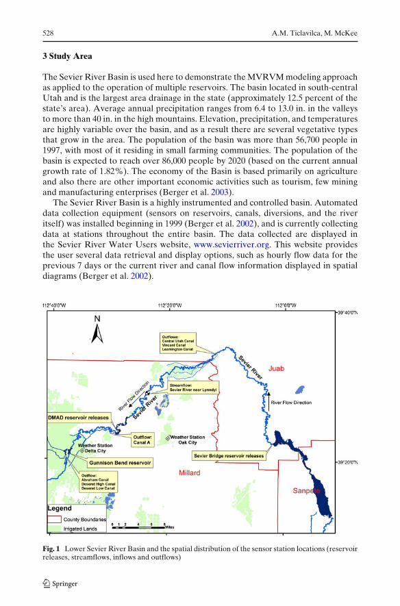
The Sevier River Basin is used here to demonstrate the MVRVM modeling approachas applied to the operation of multiple reservoirs. The basin located in south-centralUtah and is the largest area drainage in the state (approximately 12.5 percent of thestate’s area). Average annual precipitation ranges from 6.4 to 13.0 in. in the valleysto more than 40 in. in the high mountains. Elevation, precipitation, and temperaturesare highly variable over the basin, and as a result there are several vegetative typesthat grow in the area. The population of the basin was more than 56,700 people in1997, with most of it residing in small farming communities. The population of thebasin is expected to reach over 86,000 people by 2020 (based on the current annualgrowth rate of 1.82%). The economy of the Basin is based primarily on agricultureand also there are other important economic activities such as tourism, few miningand manufacturing enterprises (Berger et al. 2003).

The Sevier River Basin is a highly instrumented and controlled basin. Automateddata collection equipment (sensors on reservoirs, canals, diversions, and the riveritself) was installed beginning in 1999 (Berger et al. 2002), and is currently collectingdata at stations throughout the entire basin. The data collected are displayed inthe Sevier River Water Users website, www.sevierriver.org. This website providesthe user several data retrieval and display options, such as hourly flow data for theprevious 7 days or the current river and canal flow information displayed in spatialdiagrams (Berger et al. 2002).

Fig. 1 Lower Sevier River Basin and the spatial distribution of the sensor station locations (reservoirreleases, streamflows, inflows and outflows)

http://www.sevierriver.org


In this paper we focus on the Lower Sevier River Basin, which is regulated bythree reservoirs: Sevier Bridge (or Yuba) Reservoir, the Delta-Millard AssociationDam (DMAD) Reservoir, and Gunnison Bend Reservoir (Fig. 1).

4 Model Application to Multiple Reservoir System

The MVRVM previously described is applied to the multiple reservoir systemlocated in the Lower Sevier River Basin. Monitoring data are posted hourly tothe Sevier River website. This information enables real-time operations of reservoirreleases and canal diversions. Daily averages taken from the Sevier River databaseand the United States Geological Survey (USGS) website (http://waterdata.usgs.gov/nwis) from 2001 to 2007 were used to build the MVRVM reservoir model. Dailydata from the irrigation seasons of 2001 through 2006 were used to train the MVRVMand find the model parameters. Daily data from the 2007 irrigation season were usedto test the model.

The inputs are available past daily data collected by sensors on the reservoirs,canals, diversions, weather and the river itself. The multiple output target vectors arethe predictions of water releases 1 and 2 days ahead from Sevier Bridge and DMADreservoirs.

The USGS gauging station located on the Sevier River near Juab measures thereleases from Sevier Bridge Reservoir into the Sevier River, and the station locatedon the Sevier River bellow DMAD Reservoir measures the releases from DMADreservoir into the Sevier River (Fig. 1).

Four sensor stations are located between Sevier Bridge and DMAD reservoirs:three measure diversions to irrigation canals, and one USGS gauging station mea-sures streamflow on the Sevier River near Lynndyl. One measure diversion is madefrom DMAD reservoir to an irrigation canal called canal A. Three diversions fromGunnison Bend reservoir are measured, corresponding to irrigation releases to servethe Abraham canal, the Deseret High canal, and the Deseret Low canal.

Daily maximum and minimum temperature from Delta city wais obtained fromThe Community Environmental Monitoring Program (CEMP) website, and dailymaximum and minimum temperature from Oak City was obtained from The Na-tional Oceanic and Atmospheric Administration (NOAA).

Inputs to the MVRVM model also include past data on daily Sevier Bridgereservoir releases and data for DMAD Reservoir releases.

The inputs used in the model to predict reservoir releases are expressed as:

x = [X1d−nd, X2d−nd, X3d−nd, X4d−nd, X5d−nd

]T (9)

where,

d day of predictionnd number of days previous to the prediction timeX1d−nd diversions to the Central Utah canal, Vincent canal, Leamington canal,

canal A, Abraham canal, Deseret High canal, and Deseret Low canal.X2d−nd streamflow on the Sevier River near Lynndyl.X3d−nd Sevier Bridge reservoir releases.X4d−nd DMAD reservoir releases.X5d−nd maximum and minimum daily Temperature from Oak City and Delta City.

http://waterdata.usgs.gov/nwis

http://waterdata.usgs.gov/nwis


The multiple output target vector of the model is expressed as:

t = [R1d, R1d+1, R2d, R2d+1

]T (10)

where,

R1d prediction of Sevier Bridge reservoir release 1 day aheadR1d+1 prediction of Sevier Bridge reservoir release 2 days aheadR2d prediction of DMAD reservoir releases 1 day aheadR2d+1 prediction of DMAD reservoir releases 2 day ahead

Finally, the model can be defined as in Eq. 1 with a data set of input–output pairs{x(n), t(n)

}Nn=1, where N is the number of observations.

5 Results and Discussion

5.1 Model Selection

In Eq. 1, the basis function (��) is defined in terms of a fixed kernel function.It is necessary to choose the type of kernel function and also to determine thevalues for its associated parameter, the kernel width (Tipping 2001). As mentionedpreviously, the MVRVM model automatically sets the majority of its parameters(i.e., hyperparameters ααα and noise parameters σσσ2). The kernel width is the onlymodel parameter that must be set by the user. This is an important advantage ifwe want to compare the proposed MVRVM model with a SVM model where threeparameters (the kernel width, cost parameter and the error-insensitive parameter)must be determined by using additional procedures. For example, Hong and Pai(2007) used a simulated annealing algorithm (SA) to optimize the SVM parametersfor rainfall forecasting. Also, Pal and Goel (2007) carried out a large number of trialsto find suitable values of SVM parameters to estimate discharge and end depth in atrapezoidal channel.

The statistics used for the selection of the model are the coefficient of efficiency(E) and the correlation coefficient (R). E is equal to 1 minus the ratio of the meansquare error to the variance in the observed data. This statistic ranges from minusinfinity (poor model) to 1.0 (a perfect model) (Legates and McCabe 1999). TheR value measures the correlation between observed and predicted reservoir release.

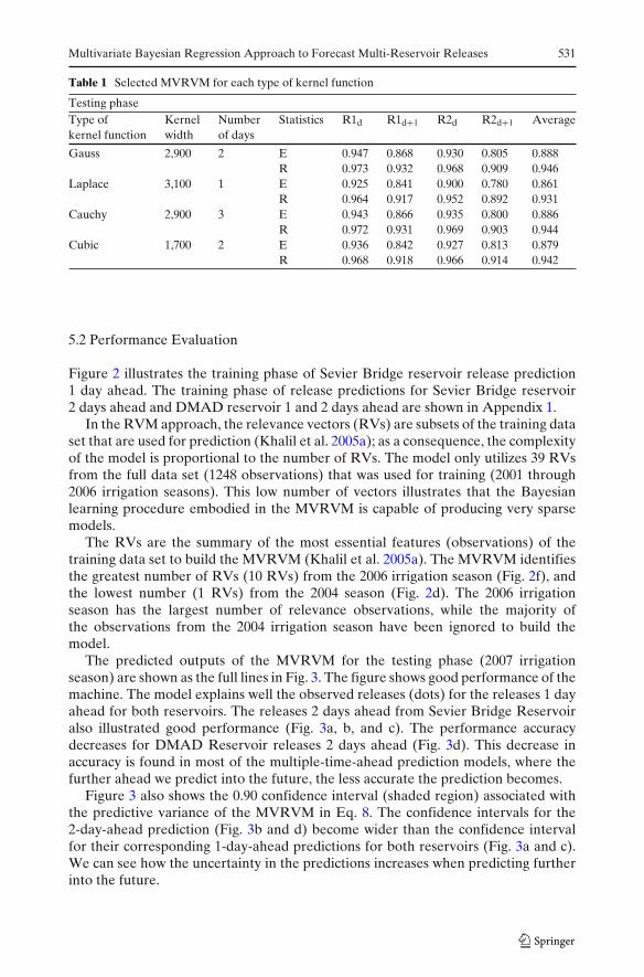
Several MVRVM models were built with variation in the type of kernel, kernelwidth and the number of days previous to the prediction time (from 1 to 5 days).The selected model was the one with the maximum E of the average outputscorresponding to the testing phase. Table 1 shows the model selected for each typeof kernel. The average results from the four kernels are equally good. The modelwith the Gaussian kernel shows slightly higher accuracy of the average results thanthe others with different kernel types. Also, the Gaussian kernel has been used byThayananthan et al. (2008) and several authors in water resources and hydrologyapplications (Khalil et al. 2005b; Tripathi and Govindaraju 2006). Therefore this typeof kernel was selected for the MVRVM model.


Table 1 Selected MVRVM for each type of kernel function

Testing phaseType of Kernel Number Statistics R1d R1d+1 R2d R2d+1 Averagekernel function width of days

Gauss 2,900 2 E 0.947 0.868 0.930 0.805 0.888R 0.973 0.932 0.968 0.909 0.946

Laplace 3,100 1 E 0.925 0.841 0.900 0.780 0.861R 0.964 0.917 0.952 0.892 0.931

Cauchy 2,900 3 E 0.943 0.866 0.935 0.800 0.886R 0.972 0.931 0.969 0.903 0.944

Cubic 1,700 2 E 0.936 0.842 0.927 0.813 0.879R 0.968 0.918 0.966 0.914 0.942

5.2 Performance Evaluation

Figure 2 illustrates the training phase of Sevier Bridge reservoir release prediction1 day ahead. The training phase of release predictions for Sevier Bridge reservoir2 days ahead and DMAD reservoir 1 and 2 days ahead are shown in Appendix 1.

In the RVM approach, the relevance vectors (RVs) are subsets of the training dataset that are used for prediction (Khalil et al. 2005a); as a consequence, the complexityof the model is proportional to the number of RVs. The model only utilizes 39 RVsfrom the full data set (1248 observations) that was used for training (2001 through2006 irrigation seasons). This low number of vectors illustrates that the Bayesianlearning procedure embodied in the MVRVM is capable of producing very sparsemodels.

The RVs are the summary of the most essential features (observations) of thetraining data set to build the MVRVM (Khalil et al. 2005a). The MVRVM identifiesthe greatest number of RVs (10 RVs) from the 2006 irrigation season (Fig. 2f), andthe lowest number (1 RVs) from the 2004 season (Fig. 2d). The 2006 irrigationseason has the largest number of relevance observations, while the majority ofthe observations from the 2004 irrigation season have been ignored to build themodel.

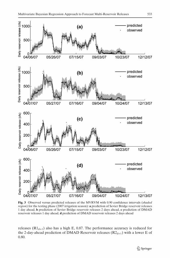
The predicted outputs of the MVRVM for the testing phase (2007 irrigationseason) are shown as the full lines in Fig. 3. The figure shows good performance of themachine. The model explains well the observed releases (dots) for the releases 1 dayahead for both reservoirs. The releases 2 days ahead from Sevier Bridge Reservoiralso illustrated good performance (Fig. 3a, b, and c). The performance accuracydecreases for DMAD Reservoir releases 2 days ahead (Fig. 3d). This decrease inaccuracy is found in most of the multiple-time-ahead prediction models, where thefurther ahead we predict into the future, the less accurate the prediction becomes.

Figure 3 also shows the 0.90 confidence interval (shaded region) associated withthe predictive variance of the MVRVM in Eq. 8. The confidence intervals for the2-day-ahead prediction (Fig. 3b and d) become wider than the confidence intervalfor their corresponding 1-day-ahead predictions for both reservoirs (Fig. 3a and c).We can see how the uncertainty in the predictions increases when predicting furtherinto the future.


Fig. 2 Plot of observed versus predicted releases of Sevier Bridge reservoir 1 day ahead, and RVs ofthe MVRVM. Training phase (2001 (a)–2006 (f) irrigation seasons)

Table 2 shows some statistics to measure MVRVM performance for both thetraining and testing phases. Again, we can see good performance of the machinein the testing phase for the 1-day-ahead prediction for both reservoir releases(R1d and R2d) with a high E, 0.95 and 0.93, respectively, for Sevier Bridge andDMAD reservoirs; and the 2-day-ahead prediction for Sevier Bridge Reservoir


Fig. 3 Observed versus predicted releases of the MVRVM with 0.90 confidence intervals (shadedregion) for the testing phase (2007 irrigation season): a prediction of Sevier Bridge reservoir releases1 day ahead, b prediction of Sevier Bridge reservoir releases 2 days ahead, c prediction of DMADreservoir releases 1 day ahead, d prediction of DMAD reservoir releases 2 days ahead

releases (R1d+1) also has a high E, 0.87. The performance accuracy is reduced forthe 2-day-ahead prediction of DMAD Reservoir releases (R2d+1) with a lower E of0.80.


Table 2 MVRVM performance using different statistics

Statistics Multivariate relevance vector machineTraining TestingR1d R1d+1 R2d R2d+1 R1d R1d+1 R2d R2d+1

Coefficient of efficiency E 0.95 0.87 0.89 0.77 0.95 0.87 0.93 0.80Correlation coefficient R 0.97 0.93 0.94 0.88 0.97 0.93 0.97 0.91Root mean square error 64.42 99.24 34.84 49.66 59.45 93.82 32.55 54.49

RMSE, cfs

5.3 Bootstrap Analysis

In order to avoid overfitting and evaluate the performance of machine learn-ing models, several authors in hydrology and water resources modeling research(El-Shafie et al. 2009; Rezaeian Zadeh et al. 2010; Shirsath and Singh 2010; Trichakiset al. 2010) calibrated their models with one training data set and evaluated theperformance of their models with a different unseen test data set. However, it isnecessary to develop models to guarantee not only high accuracy during the testperiod but also good generalization and robustness of model parameter estimationwith respect to future changes on the nature of the input data. Changes in thetraining data used to build a model may give different test results. Different sets oftraining data may produce models with very different generalization accuracies. Thebootstrap method (Efron and Tibshirani 1998) was used to explore the implicationsof the change in the nature of input data and to guarantee good generalization abilityand robustness of the MVRVM (Khalil et al. 2005b).

The bootstrap data set was generated by randomly selecting (with replacement)from the whole training data set. Because the selection is from the whole trainingdata set, there is nearly always duplication of individual points in a bootstrap dataset. In this paper, this selection process was independently repeated 1,000 times toyield 1,000 bootstrap training data sets, which are treated as independent sets (Dudaet al. 2001). For each of the bootstrap training data sets, a model was trained andevaluated over the original test data set. Figure 4 shows the bootstrap histogramsbased on 1,000 bootstrap training data sets of the E and RMSE test.

Efron and Tibshirani (1998) emphasized that it is always wise to look at thebootstrap data graphically, rather than relying entirely on a single summary statisticestimator. The bootstrap method provides information on the uncertainty in the sta-tistics estimator evaluated in the model. The width of the bootstrapping confidenceintervals provides information on the uncertainty in the model parameters. A narrowconfidence interval implies low variability of the statistics with respect to possiblefuture changes in the nature of the input data, which indicates that the model isrobust (Khalil et al. 2005b). According to Khalil et al. (2005b) a robust model isone that shows narrow confidence bounds in the bootstrap histogram, such as thoseillustrated in Fig. 4.

5.4 Comparison Between MVRVM and ANN

ANNs have been widely applied in hydrology and water resources modeling (ASCETask Committee on the Application of ANNs in Hydrology 2000a, b; Khalil et al.


Fig. 4 Bootstrap histogram of the MVRVM model for the RMSE and E test

2005d; Adeloye 2009). A comparative analysis between the developed MVRVM andANNs is performed in terms of performance and robustness. Readers interested ingreater detail regarding ANNs and their training functions are referred to Demuthet al. (2009).

The ANN model selection is similar to the MVRVM model selection describedin Section 5.1. Several feed-forward ANN models were built using different types

Table 3 Selected ANN model for each type of training function

Testing phaseType of training function Size Number Statistics R1d R1d+1 R2d R2d+1 Average

of layer of days

Quasi-Newton 3 2 E 0.942 0.867 0.898 0.777 0.871R 0.971 0.932 0.952 0.891 0.936

Conjugate gradient with 3 4 E 0.928 0.846 0.922 0.821 0.879Powell-Beale restarts R 0.964 0.922 0.961 0.908 0.939

Levenberg-Marquardt 3 5 E 0.917 0.860 0.923 0.811 0.878R 0.959 0.929 0.963 0.908 0.940

Scaled conjugate gradient 4 2 E 0.943 0.856 0.928 0.834 0.890R 0.972 0.929 0.966 0.917 0.946


of training function, sizes of layer, and numbers of days previous to the predictiontime (from 1 to 5 days). The selected model was the one with the maximum E of theaverage outputs corresponding to the testing phase. Table 3 shows the selected model

Fig. 5 Observed versus predicted releases of the ANN for the testing phase (2007 irrigation season):a prediction of Sevier Bridge reservoir releases 1 day ahead, b prediction of Sevier Bridge reservoirreleases 2 days ahead, c prediction of DMAD reservoir releases 1 day ahead, d prediction of DMADreservoir releases 2 days ahead


Table 4 ANN Performance using different Statistics

Statistics Artificial neural networkTraining TestingR1d R1d+1 R2d R2d+1 R1d R1d+1 R2d R2d+1

Coefficient of efficiency E 0.96 0.90 0.89 0.79 0.94 0.86 0.93 0.83Correlation coefficient R 0.98 0.95 0.94 0.89 0.97 0.93 0.97 0.92Root mean square error 55.47 88.21 34.50 48.29 61.77 98.11 33.02 50.29

RMSE, cfs

for each type of training function. The ANN model with the scaled-conjugated-gradient-training function shows slightly higher E and R of the average results thando the other ANN models with different training functions. Therefore this trainingfunction was chosen for the ANN model.

The observed (dots) and predicted (full lines) outputs of the ANN for thetesting phase (2007 irrigation season) are shown in Fig. 5. Table 4 shows the ANNperformance for both the training and testing phases. From Table 4 we can see thatthe performance results are fairly similar to the MVRVM performance (Table 2).

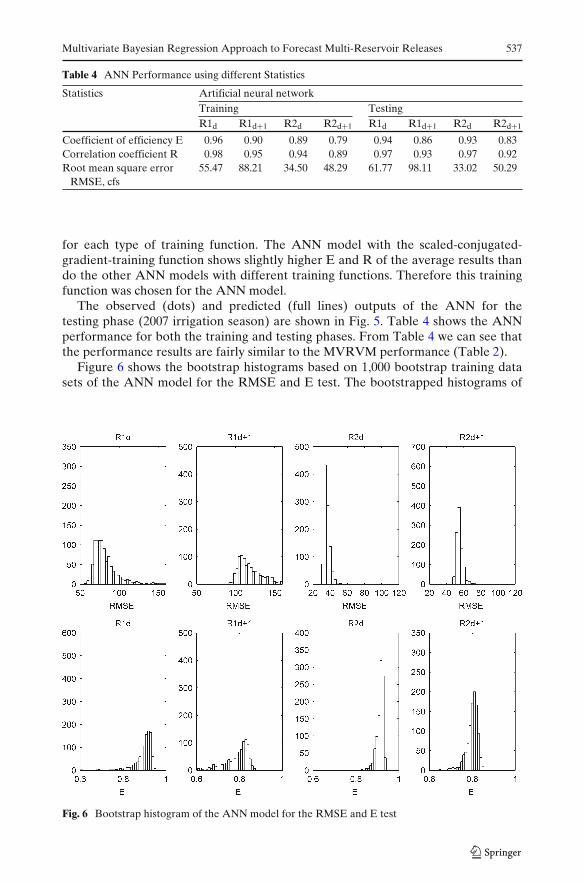
Figure 6 shows the bootstrap histograms based on 1,000 bootstrap training datasets of the ANN model for the RMSE and E test. The bootstrapped histograms of

Fig. 6 Bootstrap histogram of the ANN model for the RMSE and E test


the MVRVM model (Fig. 4) show very narrow confidence bounds in comparison tothe histograms of the ANN model (Fig. 6). Therefore, the MVRVM appears to bemore robust.

6 Summary and Conclusions

This paper presents a first attempt to use a MVRVM model to develop multiple-time-ahead predictions of daily releases from a multiple reservoir system. TheMVRVM is a regression tool extension of the RVM algorithm to produce multi-variate outputs (with predictive confidence intervals) when given a set of inputs. Themodel is illustrated by application to the Lower Sevier River near Delta, Utah. Thepredictions are water releases 1 and 2 days ahead from Sevier Bridge and DMADreservoirs.

The results show that the model learns the input–output patterns with highaccuracy consistent with the statistics for the test results. The statistical resultsindicate good performance of the model for the 1-day prediction for the releasesof Sevier Bridge and DMAD reservoirs. The performance decreased slightly for the2-day prediction of DMAD reservoir release.

The MVRVM model has the property of sparse formulation. The model onlyutilizes 39 RVs from the full data set (out of a possible 1248 observations) that wasused for training. The parsimonious structure of this empirical model is sufficientto explain the data and to avoid data over-fitting. Therefore, we can see an impor-tant advantage of the Bayesian learning procedure, which is the capability of theMVRVM to produce very sparse models.

Another important advantage of utilizing MVRVM is its generalization capabil-ities while achieving sparse representation. Generalization ability is associated withthe capability of the model to predict future system states when presented with arange of input vectors. Multiple reservoir system operation could become a difficultprocess to predict since this involves many decisions for real-time water resourcesmanagement. The model presented here ensures good generalization providingrobustness with new oncoming data.

The performance results are fairly similar by both the MVRVM and ANN. Boot-strap analysis is used to explore the robustness of the models. Narrow confidencebounds in the bootstrap histograms imply low variability of the test statistics whenpresented with a range of input vectors, which indicates that the model is robust. Thebootstrap histograms show that the MVRVM model is more robust than the ANNmodel.

In summary, the results presented in this paper have demonstrated the successfulperformance and robustness of MVRVM for multiple reservoir release forecasts.Simultaneous multiple-time-ahead release predictions from a multiple reservoirsystem have potential value to assist the reservoir operator in efficiently selectingthe real-time operation and management decisions for available water resources.

Acknowledgements The authors would like to thank the Utah Water Research Laboratory(UWRL) and the Utah Center for Water Resources Research (UCWRR) for support for thisresearch. We also thank Inga Maslova, David Stevens, Wynn Walker and Abedalrazq Khalil forhelpful comments and discussions. The authors also are grateful to Roger Hansen of the Provo,Utah, office of the U.S. Bureau of Reclamation, Bret Berger of StoneFly Technology, Inc., and JimWalker of the Sevier River Water Users Association.


Appendix 1

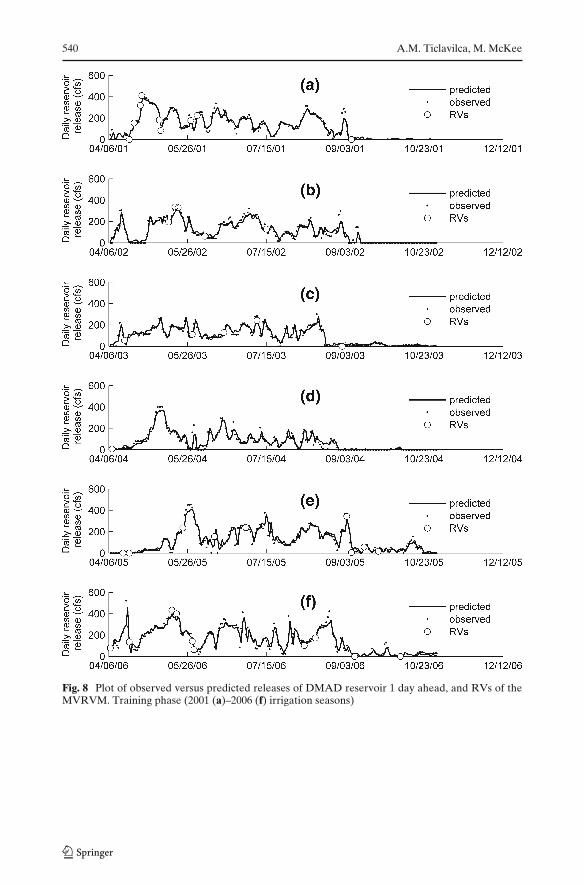
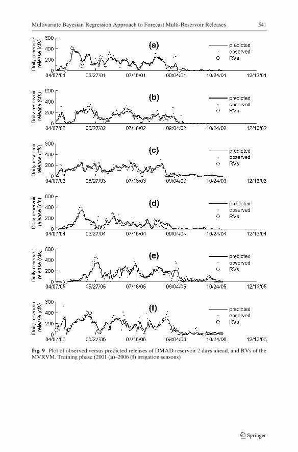
The Appendix 1 gives the training phase plots of release predictions for Sevier Bridgereservoir 1 day ahead (Fig. 7), and DMAD reservoir 1 and 2 days ahead (Figs. 8 and 9,respectively).

Fig. 7 Plot of observed versus predicted releases of Sevier Bridge reservoir 2 days ahead, and RVsof the MVRVM. Training phase (2001 (a)–2006 (f) irrigation seasons)


Fig. 8 Plot of observed versus predicted releases of DMAD reservoir 1 day ahead, and RVs of theMVRVM. Training phase (2001 (a)–2006 (f) irrigation seasons)


Fig. 9 Plot of observed versus predicted releases of DMAD reservoir 2 days ahead, and RVs of theMVRVM. Training phase (2001 (a)–2006 (f) irrigation seasons)


References

Adeloye AJ (2009) Multiple linear regression and artificial neural networks models for generalizedreservoir storage-yield-reliability function for reservoir planning. J Hydrol Eng 14(6):731–738

ASCE Task Committee on the Application of ANNs in Hydrology (2000a) Artificial neural networksin hydrology, I: preliminary concepts. J Hydrol Eng 5(2):115–123

ASCE Task Committee on the Application of ANNs in Hydrology (2000b) Artificial neural networksin hydrology, II: hydrologic application. J Hydrol Eng 5(2):124–137

Berger B, Hansen R, Hilton A (2002) Using the world-wide-web as a support system to enhancewater management. Paper presented at the 18th ICID Congress and 53rd IEC Meeting, IntComm on Irrig and Drain, Montreal, Quebec, Canada

Berger B, Hansen R, Jensen R (2003) Sevier river basin system description. Sevier River WaterUsers Association, Delta

Demuth H, Beale M, Hagan M (2009) Neural network toolbox user’s guide. The MathWorks Inc,MA

Duda RO, Hart P, Stork D (2001) Pattern classification, 2nd edn. Edited by Wiley Interscience, NYEfron B, Tibshirani R (1998) An introduction of the bootstrap, monographs on statistics and applied

probability 57. CRC Press LLC, Boca RatonEl-Shafie A, Reda Taha M, Noureldin A (2007) A neuro-fuzzy model for inflow forecasting of the

Nile river at Aswan high dam. Water Resour Manage 21:533–556El-Shafie A, Abdin AE, Noureldin A, Taha MR (2009) Enhancing inflow forecasting model at

Aswan high dam utilizing radial basis neural network and upstream monitoring stations mea-surements. Water Resour Manage 23:2289–2315

Ghosh S, Mujumdar PP (2007) Statistical downscaling of GCM simulations to streamflow usingrelevance vector machine. Adv Water Resour 31:132–146

Guldal V, Tongal H (2010) Comparison of recurrent neural network, adaptive neuro-fuzzy inferencesystem and stochastic models in Egirdir lake level forecasting. Water Resour Manage 24:105–128

Hong WC, Pai PF (2007) Potential assessment of the support vector regression technique in rainfallforecasting. Water Resour Manage 21:495–513

Khalil A, McKee M, Kemblowski MW, Asefa T (2005a) Sparse Bayesian learning machine for real-time management of reservoir releases. Water Resour Res 41:W11401

Khalil A, McKee M, Kemblowski MW, Asefa T, Bastidas L (2005b) Multiobjective analysis ofchaotic dynamic systems with sparse learning machines. Adv Water Resour 29:72–88

Khalil A, Almasari M, McKee M, Kemblowski MW, Kaluarachchi J (2005c) Applicability of statisti-cal learning algorithms in groundwater quality modeling. Water Resour Res 41:W05010

Khalil A, McKee M, Kemblowski M, Asefa T (2005d) Basin-scale water management and forecastingusing neural networks. J Am Water Resour Res 41(1):195–208

Labadie JW (2004) Optimal operation of multireservoir systems: state-of-the-art review. J WaterResour Plan Manage 130(2):93–111

Legates DR, McCabe GJ (1999) Evaluating the use of “goodness-of-fit” measures in hydrologic andhydroclimatic model validation. Water Resour Res 35(1):233–241

Lobbrecht AH, Solomatine DP (2002) Machine learning in real-time control of water systems. UrbanWater 4:283–289

Nourani V, Mehdi K, Akira M (2009) A multivariate ANN-wavelet approach for rainfall–runoffmodeling. Water Resour Manage 23:2877–2894

Pal M, Goel A (2007) Estimation of discharge and end depth in trapezoidal channel by support vectormachines. Water Resour Manage 21:1763–1780

Rezaeian Zadeh M, Amin S, Khalili D, Singh VP (2010) Daily outflow prediction by multi layerperceptron with logistic sigmoid and tangent sigmoid activation functions. Water Resour Manage24:2673–2688

Shirsath PB, Singh AK (2010) A comparative study of daily pan evaporation estimation using ANN,regression and climate based models. Water Resour Manage 24:1571–1581

Sivapragasam C, Muttil N (2005) Discharge rating curve extension—a new approach. Water ResourManage 19:505–550

Thayananthan A (2005) Template-based pose estimation and tracking of 3D hand motion. PhDthesis, Department of Engineering, University of Cambridge, Cambridge, United Kingdom

Thayananthan A, Navaratnam R, Stenger B, Torr PHS, Cipolla R (2008) Pose estimation andtracking using multivariate regression. Pattern Recogn Lett 29(8):1302–1310


Tipping ME (2001) Sparse Bayesian learning and the relevance vector machine. J Mach Learn1:211–244

Tipping M, Faul A (2003) Fast marginal likelihood maximization for sparse Bayesian models. Paperpresented at Ninth International Workshop on Artificial Intelligence and Statistics, Soc for ArtifIntel Stat, Key West, FL

Trichakis IC, Nikolos IK, Karatzas GP (2010) Artificial neural network (ANN) based modeling forkarstic groundwater level simulation. Water Resour Manage

Tripathi S, Govindaraju R (2006) On selection of kernel parameters in relevance vector machinesfor hydrologic applications. Stoch Eviron Res Risk Assess 21:747–764

World Commission on Dams (2000) Dams and development: a new framework for decision-making.Earthscan Publications Ltd, London and Sterling

Multivariate Bayesian Regression Approach to Forecast Releases from a System of Multiple Reservoirs

Documents