Multivariable direct adaptive decoupling controller using multiple models and a case study

www.scichina.cominfo.scichina.com

www.springerlink.com

Special Focus

Multivariable direct adaptive decoupling

controller using multiple models and a case study

WANG Xin1,2†, YANG Hui2 & ZHENG YiHui1

1 Center of Electrical & Electronic Engineering, Shanghai Jiao Tong University, Shanghai 200240, China;2 School of Electrical & Electronic Engineering, East China Jiao Tong University, Jiangxi 330013, China

In this paper, a multivariable direct adaptive controller using multiple models without minimum phaseassumption is presented to improve the transient response when the parameters of the system jumpabruptly. The controller is composed of multiple fixed controller models, a free-running adaptive con-troller model and a re-initialized adaptive controller model. The fixed controller models are derivedfrom the corresponding fixed system models directly. The adaptive controller models adopt the directadaptive algorithm to reduce the design calculation. At every instant, the optimal controller is chosenout according to the switching index. The interaction of the system is viewed as the measured distur-bance which is eliminated by the choice of the weighing polynomial matrix. The global convergenceis obtained. Finally, several simulation examples in a wind tunnel experiment are given to show botheffectiveness and practicality of the proposed method. The significance of the proposed method is thatit is applicable to a non-minimum phase system, adopting direct adaptive algorithm to overcome thesingularity problem during the matrix calculation and realizing decoupling control for a multivariablesystem.

multivariable, multiple models, decoupling, non-minimum phase, direct adaptive

1 Introduction

The control of a dynamic system with large uncer-tainties attracts great attention from both controltheorists and engineers. It is known that a systemwith unknown time invariant or slowly time vary-ing parameters can achieve good performance byusing conventional adaptive control[1]. However,when system boundary condition changes, a sub-system fails or a large external disturbance occurs,the parameters of the system will jump abruptly,

which always results in large parameter errors, slowreaction, slow convergence, poor transient responseand even unstable system behavior[2]. To solvethese problems, a multiple models adaptive con-troller (MMAC) is proposed.

The earliest MMAC appeared in the 1970s whenmultiple Kalman filter-based models were studiedto improve the accuracy of state estimation[3,4].However, no switching and stability results werepresented. In the 1980s two kinds of MMAC were

Received October 14, 2008; accepted May 31, 2009

doi: 10.1007/s11432-009-0128-3†Corresponding author (email: [email protected])

Supported by the National Natural Science Foundation of China (Grant Nos. 60504010, 60864004), the National High-Tech Research and

Development Program of China (Grant No. 2008AA04Z129), the Key Project of Chinese Ministry of Education (Grant No. 208071), and the

Natural Science Foundation of Jiangxi Province (Grant No. 0611006)

Citation: Wang X, Yang H, Zheng Y H. Multivariable direct adaptive decoupling controller using multiple models and a case study. Sci

China Ser F-Inf Sci, 2009, 52(7): 1165–1176, doi: 10.1007/s11432-009-0128-3

developed. One named direct switching MMACwas introduced by Fu[5], where multiple state feed-back controllers were employed to guarantee thestability of the closed loop system by the use ofswitching strategy. But the switching sequencewas predetermined and the transient response waspoor. The other named indirect switching MMACwas constructed by Middleton et al.[6], in whichmultiple convex region parameter estimators wereutilized to overcome the problem of stablizabilityof the estimated model. The choice of when andto which controller switching arises was only deter-mined by the switching index. In order to improvethe transient response, Narendra et al.[7] advancedmultiple adaptive models to identify the unknownsystem simultaneously. At any instant one bestmodel was chosen out according to the switchingindex and the corresponding controller was fired.Unfortunately, after some instants, multiple adap-tive models would converge to a neighborhood,lossing the power of multiple models when the pa-rameters jumped abruptly again. Later multiplefixed models with two adaptive models were usedto solve this problem[8,9]. The above results wereextended to the discrete-time system in ref. [10].However, all of these are dealt with a single-inputsingle-output (SISO) system and adopt the indirectadaptive algorithm based on the system parameterset, which results in the singularity problem of thematrix especially in a multivariable system[11]. Inour early work, a multiple models adaptive decou-pling controller (MMADC) is proposed for a multi-input multi-output (MIMO) system[12]. It adopteda direct adaptive algorithm to reduce the compu-tational burden and avoid the singularity prob-lem during the matrix calculation. Furthermoreit realized dynamically decoupling control by thechoice of the polynomial matrices. Unfortunatelythe system must be assumed to be of minimumphase, which has little practical utility since mostpractical processes exhibit some form of nonmini-mum phase behavior particularly when controlleddigitally[13]. For most processes, a continuousminimum phase system can be transformed intoa discrete-time nonminimum phase system whenthe sampling period is selected to be small

enough[13].In this paper, a new multiple models direct adap-

tive decoupling controller (MMDADC) without theminimum phase system assumption is presented.The control structure includes a set of multiplefixed optimal controllers, a free-running adaptivecontroller and a re-initialized adaptive controller.The effect of the fixed controllers is to provideinitial control actions to the process if its modellies in the corresponding region. The re-initializedadaptive controller utilizes the parameters of theselected controller as its initial value for the adap-tation algorithm to improve the transient response.As the value of the re-initialized controller is veryclose to that of the true optimal one, it has fasteradaptation speed than the conventional adaptivecontroller with other initial values. Therefore there-initialized adaptive controller can be used to re-place the selected ones at later stage accordingto a switching criterion in which the value of acontroller nearest to the true optimal one is se-lected. A free-running adaptive controller usingsingle model structure is also added to guaranteethe overall system stability. The main contribu-tions of this paper are: 1) the proposed methodis applicable to nonminimum phase system whichcan be extended to the computer controlled systemdirectly; 2) the interaction in the MIMO processesis viewed as measured disturbance and removed bythe choice of the weighing polynomial matrix to re-alize the decoupling control; 3) it adopts the directadaptive algorithm to reduce both computationalburden and the chances of singular matrix duringthe process of determining controller parameters;4) the global stability of the overall system and theconvergence of the tracking error to zero using thiscontrol method are theoretically proved. Severalsimulation examples in an injector driven transonicwind tunnel process show that the MMDADC canimprove the overall system performances comparedwith conventional adaptive control method and canmeet the strict requirements.

2 Description of the system

The system is a linear MIMO discrete-time system,

1166 WANG X et al. Sci China Ser F-Inf Sci | Jul. 2009 | vol. 52 | no. 7 | 1165-1176

which admits DARMA representation of the form

A(t, z−1)y(t) = B(t, z−1)u(t − k) + d(t), (1)

where u(t),y(t) are the n×1 input, output vectorsrespectively, d(t) is an n × 1 vector denoting thesteady state output response for a zero input signal.k, z−1 are time delay and unit delay operator, re-spectively, A(t, z−1),B(t, z−1) are polynomial ma-trices with comparable dimensions as follows:

A(t, z−1) = I + A1(t)z−1 + · · · + Ana(t)z−na , (2)

B(t, z−1) = B0(t) + B1(t)z−1 + · · · + Bnb(t)z−nb ,

(3)where Ai(t) and Bi(t) are time-varying parametermatrices with infrequent large jumps, B0(t) is anonsingular known matrix for any t and I is a unitmatrix. Here A(t, z−1) is assumed to be a diagonalpolynomial matrix without loss of generality.

The system satisfies the assumptions as follows:1) The system parameters are time variant with

infrequent large jumps. The period between twoadjacent jumps is large enough to keep the jump-ing parameters constant.

2) Φ(t) = [−A1(t), · · · ;B0(t), · · · ;d(t)] is thesystem model which changes in a compact set Σ .

3) The upper bounds of the orders na, nb ofA(t, z−1),B(t, z−1), and the time delay k areknown a prior.

From assumption 1), Ai(t),Bj(t),d(t) are piece-wise constant (time variant system with infrequentlarge jumping parameters). During the periodwhen no jumps happen, eq. (1) can be rewrittenas

A(z−1)y(t + k) = B(z−1)u(t) + d. (4)

To decouple the system, the interaction causedby the input uj(t) to the output yi(t), (i �= j) isviewed as the measurable disturbance and is elim-inated by the feedforward decoupling strategy. Sosystem (4) can be rewritten as

A(z−1)y(t + k) = B(z−1)u(t) + ¯B(z−1)u(t) + d,

(5)where B(z−1) = B(z−1) + ¯B(z−1). Here B(z−1)is a diagonal polynomial matrix with B(z−1) =diag[Bii(z−1)] with B0 nonsingular and ¯B(z−1) =[Bij(z−1)] with ¯Bii(z−1) = 0.

Remark 1. The u(t) in the B(z−1)u(t) isviewed as the control input to the system while theu(t) in the ¯B(z−1)u(t) is viewed as the measureddisturbance, which is eliminated by the choice ofthe weighing polynomial matrices under feedfor-ward decoupling strategy.

3 Multiple models adaptive controller

An MMAC is extended from the conventionaladaptive controller using single model. To improvethe transient response, the region where the sys-tem parameters vary is partitioned into multiplesub-regions. In every sub-region one fixed systemmodel is set up and all these models constitutethe fixed system models. The overall control sys-tem includes multiple fixed controllers, one free-running adaptive controller and one re-initializedadaptive controller. The multiple fixed controllersand the re-initialized adaptive controller are em-ployed to improve the transient response, while thefree-running adaptive controller is used to guaran-tee the stability (see Figure 1).

3.1 Foundation of the fixed system models

Definition 1. The matrix Φ, which is com-posed of the coefficient matrix of the matrix poly-nomial A(z−1), B(z−1), d, is called the systemmodel. As t changes, all of Φ(t) make up the sys-tem parameter set Σ .

Σ is partitioned into m subsets Σ ss =(1, · · · ,m) and each Σ s has the following proper-ties:

1)⋃m

s=1 Σ s ⊇ Σ , Σ s is a compact set which isnot empty, s = (1, · · · ,m).

2) For any Φ ∈ Σ s, s = 1, · · · ,m, there ex-ists a Φs ∈ Σ s and 0 � rs < ∞, satisfying‖Φ −Φs‖ � rs. Φs is called the center of the sub-set Σ s, and rs is called its radius. The existenceof rs is guaranteed by assumption 2).

From 1) and 2), it is known that the system pa-rameter set Σ is covered by multiple subsets Σ s

and every subset is covered by the center Φs andits neighbor entirely. So the centers of all subsetsare chosen out as the fixed system models to coverthe system parameter set entirely.

WANG X et al. Sci China Ser F-Inf Sci | Jul. 2009 | vol. 52 | no. 7 | 1165-1176 1167

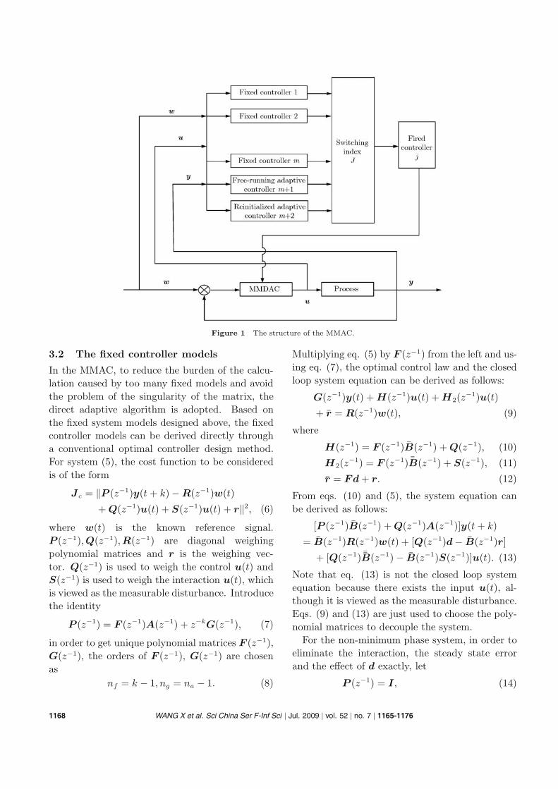
Figure 1 The structure of the MMAC.

3.2 The fixed controller models

In the MMAC, to reduce the burden of the calcu-lation caused by too many fixed models and avoidthe problem of the singularity of the matrix, thedirect adaptive algorithm is adopted. Based onthe fixed system models designed above, the fixedcontroller models can be derived directly througha conventional optimal controller design method.For system (5), the cost function to be consideredis of the form

Jc = ‖P (z−1)y(t + k) − R(z−1)w(t)

+ Q(z−1)u(t) + S(z−1)u(t) + r‖2, (6)

where w(t) is the known reference signal.P (z−1),Q(z−1),R(z−1) are diagonal weighingpolynomial matrices and r is the weighing vec-tor. Q(z−1) is used to weigh the control u(t) andS(z−1) is used to weigh the interaction u(t), whichis viewed as the measurable disturbance. Introducethe identity

P (z−1) = F (z−1)A(z−1) + z−kG(z−1), (7)

in order to get unique polynomial matrices F (z−1),G(z−1), the orders of F (z−1), G(z−1) are chosenas

nf = k − 1, ng = na − 1. (8)

Multiplying eq. (5) by F (z−1) from the left and us-ing eq. (7), the optimal control law and the closedloop system equation can be derived as follows:

G(z−1)y(t) + H(z−1)u(t) + H2(z−1)u(t)

+ r = R(z−1)w(t), (9)

where

H(z−1) = F (z−1)B(z−1) + Q(z−1), (10)

H2(z−1) = F (z−1) ¯B(z−1) + S(z−1), (11)

r = Fd + r. (12)

From eqs. (10) and (5), the system equation canbe derived as follows:

[P (z−1)B(z−1) + Q(z−1)A(z−1)]y(t + k)

= B(z−1)R(z−1)w(t) + [Q(z−1)d − B(z−1)r]

+ [Q(z−1) ¯B(z−1) − B(z−1)S(z−1)]u(t). (13)

Note that eq. (13) is not the closed loop systemequation because there exists the input u(t), al-though it is viewed as the measurable disturbance.Eqs. (9) and (13) are just used to choose the poly-nomial matrices to decouple the system.

For the non-minimum phase system, in order toeliminate the interaction, the steady state errorand the effect of d exactly, let

P (z−1) = I, (14)

1168 WANG X et al. Sci China Ser F-Inf Sci | Jul. 2009 | vol. 52 | no. 7 | 1165-1176

Q(z−1) = λI, (15)

R(z−1) = I + λB−1(1)A(1), (16)

S(z−1) = λB−1(1) ¯B(1), (17)

r = λB−1(1)d. (18)

Then, from eq. (9), another control law can bederived as

G(z−1)y(t) + [H(z−1) + H2(z−1)]u(t) + r

= R(z−1)w(t). (19)

From eqs. (19) and (5), the closed loop systemequation can be derived as

[B(z−1)B−1(1)B(1) + λA(z−1)]y(t + k)

= [B(z−1)B−1(1)B(1) + λA(1)]w(t), (20)

where λ is a constant value and decided by the de-signer to guarantee the stability of the closed loopsystem. So the forth assumption is as follows:

4) For the polynomial matrices A(z−1),B(z−1)of system (4), there must exist a constant value λ

satisfying

det[B(z−1) + λA(z−1)] �= 0, |z| � 1. (21)

From eq. (20), it is concluded that by the choice ofthe weighing polynomial matrices, the closed loopsystem can be decoupled statically.

Definition 2. The matrix Θ composed of thecoefficient matrices of G(z−1),H(z−1), r, whichis derived from system model Φ by using eqs.(21), (14)–(18), (10)–(12), is called the controllermodel. All of Θ(t) derived from Φ(t) make upthe controller parameter set Ω . The set Σ s,which is composed of the Θ(t) derived from theΦ(t) ∈ Σ s, (s = 1, · · · m), is called controller pa-rameter subset and Θs, which is derived from theΦs ∈ Σ s, (s = 1, · · · m), is called the center of thesubset Σ s.

3.3 Free-running adaptive controller

For the free-running direct adaptive controller, therecursive estimation algorithm is described as

y(t + k) = G(z−1)y(t) + H ′(z−1)u(t)

+ H ′2(z

−1)u(t) + r′, (22)

θi(t) = θi(t − 1) + a(t)X(t − k)

1 + X(t − k)T X(t − k)

× [yi(t)T − X(t − k)Tθi(t − 1)] (23)

with

H ′(z−1) = F (z−1)B(z−1), (24)

H ′2(z

−1) = F (z−1) ¯B(z−1), (25)

r′ = F (1)d, (26)

where X(t) = [y(t)T, · · · ;u(t)T, · · · ; 1]T is thedata vector, Θ = [θ1, · · · , θn] is the controller par-ameter matrix and θi = [g0

i1, · · · , g0in; g1

i1, · · · , g1in,

· · · ;h0i1, · · · , h0

in; · · · ]T, i = 1, 2, · · · , n, respectively.The scalar a(t) is set to avoid the singularity prob-lem of the estimation H(0), i.e. B(0). If H(0)is singular and u(t) cannot be achieved, let a(t)be equal to another constant value in the intervalσ < a(t) < 2 − σ, 0 < σ < 1 to estimate H(0)again[14].

3.4 Re-initialized direct adaptivecontroller

For the re-initialized direct adaptive controller, ifit is not the optimal controller chosen out accord-ing to the switching index, its initial value shouldbe re-initialized as the optimal controller parame-ter to improve the transient response, otherwise itshould be estimated using eqs. (22) and (23) likethe free-running one.

3.5 Multiple models direct adaptivecontrollers

Definition 3. The multiple controller mod-els are composed of m fixed controller models Θs,s = 1, · · · ,m, one free-running adaptive controllermodel Θm+1 and one re-initialized adaptive con-troller model Θm+2. The free-running adaptivecontroller model Θm+1 is used to guarantee thestability of the system and the re-initialized adap-tive controller model Θm+2 is used to improve thetransient response substantially.

To an MMDADC, the switching index is as fol-lows:

Js = ‖es(t)‖2 = ‖y(t) − ys(t)‖2, (27)

where ys(t) = ΘTs X(t − k) is the output of the

model s, es(t) is output error between the real sys-tem and the model s. Let j = argmin(Js), s =1, · · · ,m,m + 1,m + 2 corresponds to the modelwhose output error is minimum . Then Θ j is cho-sen to be the optimal controller.

WANG X et al. Sci China Ser F-Inf Sci | Jul. 2009 | vol. 52 | no. 7 | 1165-1176 1169

The optimal control law can be obtained from

G(z−1)y(t)+ ˆH(z−1)u(t)+ˆr = R(z−1)w(t) (28)

with H(z−1) = F (z−1)B(z−1) + Q(z−1)S(z−1).The weighing polynomial matrices R(z−1),Q(z−1),S(z−1), r are chosen as

Q(z−1) = λI, (29)

R(z−1) = I + λH ′−1(1)[I − G(1)], (30)

S(z−1) = λH ′−1(1)H ′2(1), (31)

r = λH ′−1(1)r′. (32)

Algorithm 1.1) Partition the system model into m fixed mod-

els as in section 3.1.2) Design the corresponding fixed controllers by

eq. (9).3) Form the data vector X(t) as in eq. (23).4) Estimate Θm+1 and Θm+2 by (23);5) Choose the best controller j based on the

switching index (27).6) Initialize Θm+2 as Θm+2(t) = Θ j if j �= m+2.7) Set the fired controller at Θ(t) = Θ j and

obtain u(t) as in eq. (28) accordingly.8) For t = t + 1, go to Step 3).

Remark 2. To a minimum phase system,a multivariable MMAC is designed to decouplethe system with arbitrary poles placement in ref.[12]. Accordingly the SISO MMAC for a minimumphase system can be found in ref. [10].

4 Global convergence analysis

Lemma 1. Define the generalized output er-ror vector as

e(t + k) = P (z−1)y(t + k) − R(z−1)w(t)

+ Q(z−1)u(t) + S(z−1)u(t) + r. (33)

For any model s ∈ (1, · · · ,m,m + 1,m + 2), wehave

[B(z−1)B−1(1)B(1) + λA(z−1)]y(t + k)

= B(z−1)B−1(1)B(1)e(t + k)

+ B(z−1)B−1(1)B(1)R(z−1)w(t), (34)

[B(z−1) + λA(z−1)B−1(1)B(1)]u(t)

= A(z−1)e(t + k) + A(z−1)R(z−1)w(t)

− [Ar + d]. (35)

Proof. For any model, it has the same de-scription of the system and the generalized outputerror. Substituting eq. (5) into eq. (33), we get

e(t + k) = y(t + k) − R(z−1)w(t)

+ [Q(z−1) + S(z−1)]u(t) + r

= y(t + k) − R(z−1)w(t)

+ [λB−1(1)B(1)]u(t) + r. (36)

From weighing polynomial matrices (14)–(18), eq.(34) follows. Similarly, substituting eq. (5) into eq.(35) and using weighing polynomial matrix (14)–(18), we have eq. (35).

Theorem 1. Under assumptions 1)–3), if al-gorithm (22) is applied to the system (5), then{y(t)}, {u(t)} are bounded and limt→∞ ‖e(t)‖ = 0.

Proof.1) If limt→∞ esi

(t)2 �= 0, s = 1, · · · ,m, meaningthat whenever a fixed model is adopted, the conver-gence property cannot be guaranteed, then theremust exist a constant value εi = min1�s�m esi

(t).For the adaptive controller m+1, recursive esti-

mation algorithm (20) has the property

limt→∞

em+1i

(t)2

1 + X(t − k)TX(t − k)= 0. (37)

Then there must exist an instant ts. When t > ts,we have

em+1i

(t)2

1 + X(t − k)TX(t − k)

� εi(t)2

1 + X(t − k)TX(t − k),

i = 1, · · · , n. (38)

According to the switching index, considering allmodels have the same data vector X(t − k), wehave

ei(t)2

1 + X(t − k)TX(t − k)

�e

m+1i

(t)2

1 + X(t − k)TX(t − k), (39)

so

limt→∞

ei(t)2

1 + X(t − k)TX(t − k)= 0, i = 1, · · · , n.

(40)

1170 WANG X et al. Sci China Ser F-Inf Sci | Jul. 2009 | vol. 52 | no. 7 | 1165-1176

By Lemma 1, the stability of [B(z−1)B−1(1)B(1)+λA(z−1)] and wi(t), di is bounded; thus[14]

|yi(t)| � K1 + K2 max1�τ�t1�j�n

|ej(τ)|,

0 < K1,K2 < ∞,

1 � t � N, i = 1, · · · , n, (41)

|ui(t − k)| � K3 + K4 max1�τ�t1�j�n

|ej(τ)|,

0 < K3,K4 < ∞,

1 � t � N, i = 1, · · · , n. (42)

According to Lemma 3.1 in ref. [14], {y(t)}, {u(t)}are bounded and limt→∞ ‖e(t)‖ = 0.

2) If limt→∞ esi(t)2 = 0, s = 1, · · · ,m, which

means that there exists at least one fixed con-troller model whose controller parameter matrixΘs equals the real value of the system Θ0 orΘs−Θ0 is orthogonal to the data vector X(t−k).At that moment, Js = 0 and Θs is chosen to bethe controller parameter matrix. Then it reducesto the single model case and switching stops. Us-ing a similar argument above, by Lemma 1, thestability of [B(z−1)B−1(1)B(1) + λA(z−1)] andwi(t), di is bounded, and by Lemma 3.1 in ref. [14],{y(t)}, {u(t)} are bounded and ‖e(t)‖=‖es(t)‖=0.

Considering the above cases together, the resultfollows.

Remark 3. For a minimum system in ref.[12], because B(z−1) is stable, eq. (42) can bederived from eqs. (5) and (41) directly. However,for a nonminimum system, the conclusion cannotbe derived directly and Lemma 1 must be used.

5 Verification by the wind tunnel experi-ment

The 2.4 m×2.4 m injector driven transonic windtunnel in the China Aerodynamics Research andDevelopment Center (CARDC) is the biggest windtunnel in Asia[15]. It is a very important device fornational defense and civil aviation. The wind tun-nel requires that 1) in the initial stage, the responsetime should be no longer than 7.0 s; 2) in the ex-periment stage, the steady state tracking errors arewithin 0.2% in 0.8 s and the overshoot should beavoided[16]. In a 1.5 m wind tunnel (FFA-T1500)

in Sweden, several separate SISO models are usedfor controlling[17]. A 1.6 m×2 m wind tunnel inNetherlands is regarded as a second-order systemand a PID controller is adopted[18], whose Machnumber is controlled by a predictive controller[19].In the USA, a system of self-organization neuralnetworks has been developed and tested to clus-ter, predict and control the Mach number of a 16-foot wind tunnel in NASA[20]. However, the sizeand mechanism of the above wind tunnels are alldifferent from that in China, so the controller de-sign method cannot be applied directly. For the2.4 m×2.4 m transonic wind tunnel in CARDC,two SISO stable linear reduced order models areestablished and two PID controllers are designedto control the Mach number and the stagnationtotal pressure respectively[16]. But when the Machnumber in the test section is larger than 0.8, the in-teraction becomes stronger and a multivariable de-coupling controller is needed[21]. In ref. [15], a mul-tivariable feedforward decoupler with four fixed PIcontrollers was designed to solve this problem. Butwhen the Mach number ranges from 0.8 to 0.9, 1.0,1.2, the parameters of the wind tunnel will jumpaccordingly. The poor transient response cannotsatisfy the high requirements of the wind tunnelabove. So some special controller structures andcontrol algorithms are needed.

The 2.4 m×2.4 m injector driven transonic windtunnel is the biggest intermittent wind tunnel inAsia. It is constructed for the aeronautical re-search aim of the CARDC and has many operationcases[16]. In one of the wind tunnel experiments,the Mach number in test section and the stagnationtotal pressure were required to track some desiredvalues. After the stable flowing field is established,the Mach number in test section was required tovary from 0.8 to 1.2 with ΔM = 0.1 using theplenum exhaust valve, while the stagnation totalpressure was set at 1.5 constantly using the mainexhaust hydraulic servo valve, as shown in Figure2.

Because the experiment time of the wind tunnelis limited, the control objective is to ensure that[15]

1) In the initial stage, the time to establish thestable flowing field at the beginning of the initial

WANG X et al. Sci China Ser F-Inf Sci | Jul. 2009 | vol. 52 | no. 7 | 1165-1176 1171

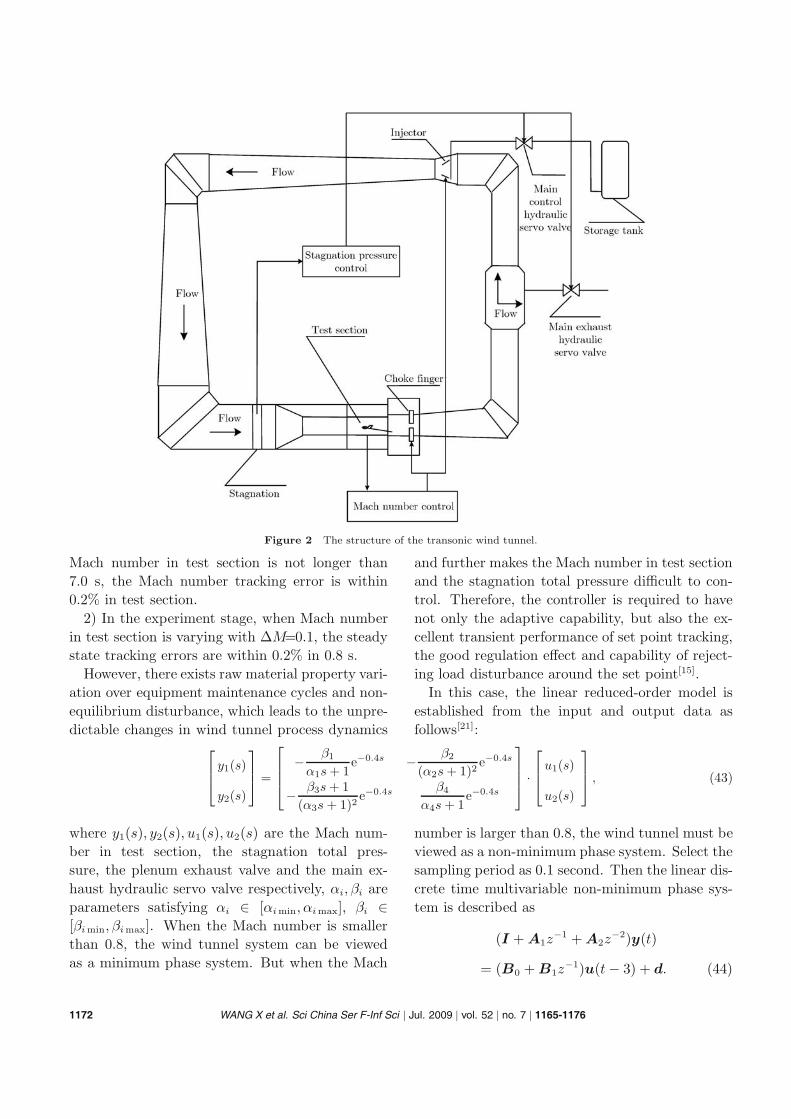
Figure 2 The structure of the transonic wind tunnel.

Mach number in test section is not longer than7.0 s, the Mach number tracking error is within0.2% in test section.

2) In the experiment stage, when Mach numberin test section is varying with ΔM=0.1, the steadystate tracking errors are within 0.2% in 0.8 s.

However, there exists raw material property vari-ation over equipment maintenance cycles and non-equilibrium disturbance, which leads to the unpre-dictable changes in wind tunnel process dynamics

and further makes the Mach number in test sectionand the stagnation total pressure difficult to con-trol. Therefore, the controller is required to havenot only the adaptive capability, but also the ex-cellent transient performance of set point tracking,the good regulation effect and capability of reject-ing load disturbance around the set point[15].

In this case, the linear reduced-order model isestablished from the input and output data asfollows[21]:

⎡

⎢⎣

y1(s)

y2(s)

⎤

⎥⎦ =

⎡

⎢⎢⎣

− β1

α1s + 1e−0.4s − β2

(α2s + 1)2e−0.4s

− β3s + 1(α3s + 1)2

e−0.4s β4

α4s + 1e−0.4s

⎤

⎥⎥⎦ ·

⎡

⎢⎣

u1(s)

u2(s)

⎤

⎥⎦ , (43)

where y1(s), y2(s), u1(s), u2(s) are the Mach num-ber in test section, the stagnation total pres-sure, the plenum exhaust valve and the main ex-haust hydraulic servo valve respectively, αi, βi areparameters satisfying αi ∈ [αi min, αi max], βi ∈[βi min, βi max]. When the Mach number is smallerthan 0.8, the wind tunnel system can be viewedas a minimum phase system. But when the Mach

number is larger than 0.8, the wind tunnel must beviewed as a non-minimum phase system. Select thesampling period as 0.1 second. Then the linear dis-crete time multivariable non-minimum phase sys-tem is described as

(I + A1z−1 + A2z

−2)y(t)

= (B0 + B1z−1)u(t − 3) + d. (44)

1172 WANG X et al. Sci China Ser F-Inf Sci | Jul. 2009 | vol. 52 | no. 7 | 1165-1176

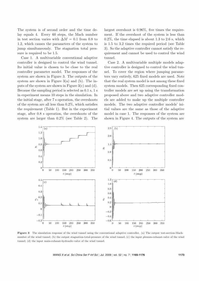
The system is of second order and the time de-lay equals 4. Every 60 steps, the Mach numberin test section varies with ΔM = 0.1 from 0.8 to1.2, which causes the parameters of the system tojump simultaneously. The stagnation total pres-sure is required to be 1.5.

Case 1. A multivariable conventional adaptivecontroller is designed to control the wind tunnel.Its initial value is chosen to be close to the realcontroller parameter model. The responses of thesystem are shown in Figure 3. The outputs of thesystem are shown in Figure 3(a) and (b). The in-puts of the system are shown in Figure 3(c) and (d).Because the sampling period is selected as 0.1 s, 1 sin experiment means 10 steps in the simulation. Inthe initial stage, after 7 s operation, the overshootsof the system are all less than 0.2%, which satisfiesthe requirement (Table 1). But in the experimentstage, after 0.8 s operation, the overshoots of thesystem are larger than 0.2% (see Table 2). The

largest overshoot is 0.96%, five times the require-ment. If the overshoot of the system is less than0.2%, the time elapsed is about 1.3 to 2.6 s, whichis 1.5 to 3.2 times the required period (see Table3). So the adaptive controller cannot satisfy the re-quirement and cannot be used to control the windtunnel.

Case 2. A multivariable multiple models adap-tive controller is designed to control the wind tun-nel. To cover the region where jumping parame-ters vary entirely, 625 fixed models are used. Notethat the real system model is not among these fixedsystem models. Then 625 corresponding fixed con-troller models are set up using the transformationproposed above and two adaptive controller mod-els are added to make up the multiple controllermodels. The two adaptive controller models’ ini-tial values are the same as those of the adaptivemodel in case 1. The responses of the system areshown in Figure 4. The outputs of the system are

Figure 3 The simulation response of the wind tunnel using the conventional adaptive controller. (a) The output test-section-Mach-

number of the wind tunnel; (b) the output stagnation-total-pressure of the wind tunnel; (c) the input plenum-exhaust-valve of the wind

tunnel; (d) the input main-exhaust-hydraulic-valve of the wind tunnel.

WANG X et al. Sci China Ser F-Inf Sci | Jul. 2009 | vol. 52 | no. 7 | 1165-1176 1173

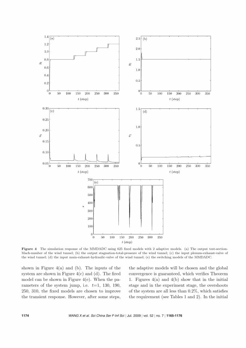
Figure 4 The simulation response of the MMDADC using 625 fixed models with 2 adaptive models. (a) The output test-section-

Mach-number of the wind tunnel; (b) the output stagnation-total-pressure of the wind tunnel; (c) the input plenum-exhaust-valve of

the wind tunnel; (d) the input main-exhaust-hydraulic-valve of the wind tunnel; (e) the switching models of the MMDADC.

shown in Figure 4(a) and (b). The inputs of thesystem are shown in Figure 4(c) and (d). The firedmodel can be shown in Figure 4(e). When the pa-rameters of the system jump, i.e. t=1, 130, 190,250, 310, the fixed models are chosen to improvethe transient response. However, after some steps,

the adaptive models will be chosen and the globalconvergence is guaranteed, which verifies Theorem1. Figures 4(a) and 4(b) show that in the initialstage and in the experiment stage, the overshootsof the system are all less than 0.2%, which satisfiesthe requirement (see Tables 1 and 2). In the initial

1174 WANG X et al. Sci China Ser F-Inf Sci | Jul. 2009 | vol. 52 | no. 7 | 1165-1176

stage, when the overshoot of the system is less than0.2%, the time is about 1 s, which is much shorterthan that in case 1 and 6 s can be saved (see Table4).

Table 1 The overshoot after 7 s operation (%)

Mach number in test Stagnation total pressure

section y1 y2

Case 1 5 × 10−2 1 × 10−2

Case 2 2 × 10−7 8 × 10−8

Table 2 The overshoot after 0.8 s operation (%)

Mach=0.9 Mach=1.0 Mach=1.1 Mach=1.2

y1 y2 y1 y2 y1 y2 y1 y2

Case 1 0.93 0.77 0.6 0.91 0.18 0.96 0.26 0.91

Case 2 0.19 0.0893 0.18 0.0874 0.15 0.0221 0.16 0.0678

Table 3 The time elapsed when the overshoot is less than 0.2%

(s)

Mach=0.9 Mach=1.0 Mach=1.1 Mach=1.2

y1 y2 y1 y2 y1 y2 y1 y2

Case 1 2.6 1.7 1.8 1.3 1.4 1.4 1.3 2.4

Case 2 0.8 0.3 0.8 0.5 0.7 0.5 0.7 0.6

Table 4 The time elapsed when the overshoot is less than 0.2%

(s)

Mach number in test Stagnation total pressure

section y1 y2

Case 1 5.3 4.0

Case 2 1.0 0.9

The results show that the transient response inFigure 4 is much better than that in Figure 3 es-pecially when the parameters jump abruptly. The

MMAC algorithm works quite satisfactorily.

6 Conclusion

In this paper, an MMDADC was designed on theMIMO discrete-time LTV system without the as-sumption of non-minimum phase system. In MM-DADC design, the interactions in the MIMO sys-tem were viewed as measured disturbance andeliminated by the use of feedforward strategy. Thecontroller was composed of multiple fixed controllermodels, a free-running adaptive controller modeland a re-initialized adaptive controller model. Thefixed controller models were derived from the corre-sponding fixed system models directly and provedto cover the controller parameter set with theirneighborhoods. A free-running adaptive controllerwas added to guarantee the overall system stabil-ity while the re-initialized adaptive controller wasutilized to improve the convergence speed. Basedon the switching index, the optimal controller waschosen out, which guaranteed the global conver-gence of the system. The applications of thismethod to the 2.4 m×2.4 m injector driven tran-sonic wind tunnel process had demonstrated its ef-fectiveness and practicality. It is noted, however,both Schemes 2 and 3 had 625 fixed controllers toguarantee the system performances that may posea big obstacle to the application of the method tovarious industry processes. The work to reduce thenumber of the fixed controllers plus the extensionof the method to the nonlinear system would bereported later.

1 Astrom K J, Wittenmark B. On self-tuning regulators. Auto-

matica, 1973, 9(2): 195–199

2 Goodwin G C, Hill D J, Palaniswami M. A perspective on con-

vergence of adaptive control algorithms. Automatica, 1984,

20(5): 519–531

3 Lainiotis D G. Partitioning a unifying framework for adaptive

system. I: Estimation. Proc IEEE, 1976, 64(8): 1126–1143

4 Athans M, Castanon D, Dunn K, et al. The stochastic control

of the F-8C aircraft using a multiple model adaptive control

(MMAC) method part I: Equilibrium flight. IEEE Trans Au-

tom Control, 1977, 22(5): 768–780

5 Fu M Y, Barmish B R. Adaptive stabilization of linear sys-

tems via switching control. IEEE Trans Autom Control, 1986,

31(12): 1097–1103

6 Middleton R H, Goodwin G C, Hilland D J, et al. Design

issues in adptive control. IEEE Trans Autom Control, 1988,

33(1): 50–58

7 Narendra K S, Balakrishnan J. Improving transient response of

adaptive control systems using multiple models and switching.

IEEE Trans Autom Control, 1994, 39(9): 1861–1866

8 Narendra K S, Balakrishnan J, Ciliz M K. Adaptation and

learning using multiple models, switching and tuning. IEEE

Control Syst Mag, 1995, 15(3): 37–51

9 Narendra K S, Balakrishnan J. Adaptive control using multiple

models. IEEE Trans Autom Control, 1997, 42(2): 171–187

10 Narendra K S, Xiang C. Adaptive control of discrete-time

WANG X et al. Sci China Ser F-Inf Sci | Jul. 2009 | vol. 52 | no. 7 | 1165-1176 1175

systems using multiple models. IEEE Trans Autom Control,

2000, 45(9): 1669–1686

11 Wittenmark B, Astrom K J. Practical issues in the implemen-

tation of self-tuning control. Automatica, 1984, 20(5): 595–

605

12 Wang X, Li S Y, Cai W J, et al. Multi-model direct adaptive

decoupling control with application to the wind tunnel. ISA

Trans, 2005, 44(1): 131–143

13 Clark D W. Self-tuning control of nonminimum-phase systems.

Automatica, 1984, 20(3): 501–517

14 Goodwin G C, Ramadge P J, Caines P E. Discrete-time mul-

tivariable adaptive control. IEEE Trans Autom Control, 1980,

25(3): 449–456

15 Zhang G J, Chai T Y, Shao C. A synthetic approach for control

of intermittent wind tunnel. In: Proceedings of the American

Control Conference, New Mexico, 1997. 203–207

16 Yu W, Zhang G J. Modelling and controller design for 2.4 m

injector powered transonic wind tunnel. In: Proceedings of

the American Control Conference, New Mexico, 1997. 1544–

1545

17 Nelson D M. Wind tunnel computer control system and in-

strumentation. In: The 35th International Instrumentation

Symposium, Orlando. 1989. 87–101

18 Pels A F. Closed-loop Mach number control in a transonic

wind tunnel. Journal A, 1989, 30(1): 25–32

19 Soeterboek R A M, Pels A F, Verbruggen H B, et al. A pre-

dictive controller for the Mach number in a transonic wind

tunnel. IEEE Control Syst Mag, 1991, 11(1): 63–72

20 Motter M A, Principe J C. Neural control of the NASA Lang-

ley 16-foot transonic tunnel. In: Proceedings of the American

Control Conference, New Mexico, 1997. 662–663

21 CARDC. Measurement and Control System Design in High

and Low Speed Wind Tunnel (in Chinese). Beijing: National

Defence Industry Press, 2002

1176 WANG X et al. Sci China Ser F-Inf Sci | Jul. 2009 | vol. 52 | no. 7 | 1165-1176