Multitasking network with fast noise

Multitasking network with fast noise.

Elena Agliari ∗, Adriano Barra †, Andrea Galluzzi ‡, Marco Isopi §

April 17, 2013

Abstract

We consider the multitasking associative network in the low-storagelimit and we study its phase diagram with respect to the noise level Tand the degree d of dilution in pattern entries. We find that the sys-tem is characterized by a rich variety of stable states, among which purestates, parallel retrieval states, hierarchically organized states and sym-metric mixtures (remarkably, both even and odd), whose complexity in-creases as the number of patterns P grows. The analysis is performedboth analytically and numerically: Exploiting techniques based on par-tial differential equations, allows us to get the self-consistencies for theorder parameters. Such self-consistence equations are then solved and thesolutions are further checked through stability theory to catalog their or-ganizations into the phase diagram, which is completely outlined at theend. This is a further step toward the understanding of spontaneous par-allel processing in associative networks.

1 Introduction

The paradigm, introduced almost three decades ago by Amit, Gutfreund andSompolinsky [1, 2], of analyzing neural networks through techniques stemmedfrom statistical mechanics of disordered systems (mainly the celebrated ReplicaTrick [3] for the Hopfield model [4]) has been so prolific that its applications wentfar beyond Artificial Intelligence and Robotics, overlapping Statistical Inference[5], System Biology [6], Financial Market planning [7], Theoretical Immunology[8] and much more.As a result, research in this field is under continuous development, ranging fromthe diverse applications outlined above, to an ever deeper understanding ofthe core-theory behind. For the sake of reaching results closer to experimentalneuroscience outcomes, scientists involved in the field tried to bypass the rathercrude mean field description of a fully connected network of interacting neurons,embedding them in diluted topologies as Erdos-Renyi graphs [9], small-worlds[10] or even finitely connected graphs [11]. The main point was showing ro-bustness of the mean-field paradigm even in these diluted, and in some sense‘closer to biology”, versions and this was indeed successfully achieved (with the

∗Universita di Parma, Dipartimento di Fisica and INFN Gruppo di Parma, Italy†Sapienza Universita di Roma, Dipartimento di Fisica and GNFM Gruppo di Roma, Italy‡Sapienza Universita di Roma, Dipartimento di Matematica, Italy§Sapienza Universita di Roma, Dipartimento di Matematica, Italy

1

arX

iv:1

304.

4488

v1 [

cond

-mat

.dis

-nn]

16

Apr

201

3

exception of too extreme degrees of dilution, where the associative capacities ofthe network trivially break down).

Recently, a mapping between Hopfield networks and Boltzmann machines[12, 13] allowed the introduction of dilution into associative networks from a dif-ferent perspective with respect to standard link removal a la Sompolinsky [9] ora la Coolen [10, 11]. In fact, while in their papers these authors perform dilutiondirectly on the Hopfield network, through the equivalence with Boltzmann ma-chine, one may perform link dilution on the Boltzmann machine and then mapback the latter into the associative Hopfield-like network checking for its emerg-ing properties [14]. Remarkably, the resulting model still works as an associativeperformer, as the Hebbian structure is preserved, but its capabilities are quitedifferent from the standard scenario. In particular, the resulting associative net-work may still be fully-connected but the stored patterns of information displayentries which, beyond coding information through digital values ±1, can alsobe blank [14, 15]. In fact, any missing link in the bipartite Boltzmann machinecorresponds to a blank entry in the related pattern of the associative network.Now, while standard (i.e., performed directly on the Hopfield network) dilu-tion does not change qualitatively the system performances, the behavior of thesystem resulting from hidden (i.e., performed on the underlying Boltzmann ma-chine) dilution becomes ‘multitasking” because retrieval of a single pattern, sayξ1, does not exhaust the whole neurons, and the ones coupled with the ξ1 blankentries are free to align with ξ2, whose entries will partially be blank as well,hence eliciting, in turn, the retrieval of ξ3 and so on up to a parallel logarithmic(with respect to the volume of the network N) load of all the stored patterns.As a consequence, by tuning the degree of dilution in the hidden Boltzmannnetwork and the level of noise in the directed network, the system exhibits avery rich phase diagram, whose investigation is the subject of the present work.

The paper is organized as follows. In section 2, we review the multitaskingnetworks introduced in [14] highlighting their main features and providing arigorous solution for their thermodynamics through a novel technique basedon mapping the statistical mechanical problem into a diffusion problem andthen solving the latter through standard partial differential equation methods.In section 3 solutions obtained in the previous section are investigated. Inparticular, we discuss the emergence of spurious states for these multitaskingnetworks. Then, in section 4 we describe the analytical technique used to studythe stability of the retrieval states, which are found to be solutions of the system.Exact analytical investigations and numerical results are presented in section5 and a very rich phase diagram, where different emergent behaviors in theorganization of the neural states are proved. Finally, section 6 is devoted to asummary and a discussion of the results which are successfully checked againstMonte Carlo simulations.

2 The multitasking associative network

In the conventional Hopfield model (see, e.g., [1, 16]), one considers a network ofN neurons, where each neuron σi can take two states, namely, σi = +1 (firing)and σi = −1 (quiescent). Neuronal states are given by the set of variablesσσσ = (σ1, ..., σN ). Each neuron is located on a node of a complete graph and thesynaptic connection between two arbitrary neurons, say, σi and σj , is defined

2

by the following Hebb rule [1]:

Jij =1

N

P∑µ=1

ξµi ξµj , (1)

where ξξξµ = (ξ1, ..., ξN ) denotes the set of memorized patterns, each specifiedby a label µ = 1, ..., P . The entries are dichotomic, i.e., ξµi ∈ {+1,−1}, chosenrandomly and independently with equal probability, namely, for any i and µ,

P (ξµi ) =1

2(δξµi −1 + δξµi +1), (2)

where the Kronecker delta δx equals 1 iff x = 0, otherwise it is zero. Patternsare assumed as quenched, that is, the performance of the network is analyzedkeeping the synaptic values fixed.

The Hamiltonian describing this system is

HN (σ, ξσ, ξσ, ξ) = −N∑i=1

N∑i>j=1

Jijσiσj = − 1

2N

N,N∑i,j=1j 6=i

P∑µ=1

ξµi ξµj σiσj , (3)

so that the signal (i.e. the field) acting on neuron i is

hi(σ, ξσ, ξσ, ξ) =

N∑j=1j 6=i

Jijσj . (4)

The evolution of the system is ruled by a stochastic dynamics, according towhich the probability that the activity of a neuron i assumes the value σi is

P (σi;σ, ξσ, ξσ, ξ, β) =1

2[1 + tanh(βhiσi)], (5)

where β tunes the level of noise such that for β → 0 the system behaves com-pletely randomly, while for β →∞ it becomes noiseless and deterministic; noticethat the noiseless limit of Eq. (5) is σi(t+ 1) = sign [hi(t)].

The main feature of the model described by Eqs. (3) and (5) is its abilityto work as an associative memory. More precisely, the patterns are said tobe memorized if each of the network configurations σi = ξµi for i = 1, ..., N ,for everyone of the P patterns labeled by µ, is a fixed point of the dynamics.Introducing the overlap mµ between the state of neurons σσσ and one of thepatterns ξξξµ, as

mµ =1

N(σ · ξµσ · ξµσ · ξµ) =

1

N

N∑i=1

σiξµi , (6)

such a pattern is said to be retrieved if, in the thermodynamic limit, mµ = O(1).Given the definition (6), the Hamiltonian (3) can also be written as

HN (σ, ξσ, ξσ, ξ) = −NP∑µ=1

(mµ)2 + P = −Nmmm2 + P. (7)

3

The analytical investigation of the system is usually carried out in the ther-modynamic limit N → ∞, consistently with the fact that real networks arecomprised of a very large number of neurons. Dealing with this limit, it is con-venient to specify the relative number of stored patterns, namely P/N and todefine the ratio α = limN→∞ P/N . The case α = 0, corresponding to a numberP of stored patterns scaling sub-linearly with respect to the amount of perform-ing neurons N , is often referred to as “low storage”. Conversely, the case offinite α is often referred to as “high storage”. In particular, in the former case(α = 0), the overall behavior of the standard Hopfield model is ruled only bythe noise T ≡ 1/β and the so-called pure-state ansatz

mmm = (m, 0, ..., 0), (8)

always corresponds to a stable solution for T < 1; the order in the entriesis purely conventional and here we assume that the first pattern is the onestimulated.

Let us now move on and generalize the system described above in order toaccount for the existence of blank entries in the patterns ξ’s. More precisely, wereplace Eq. (2) by

P (ξµi ) =1− d

2δξµi −1 +

1− d2

δξµi +1 + dδξµi , (9)

where d encodes the degree of “dilution” in pattern entries. Patterns are stillassumed as quenched and, of course, the definitions of the Hamiltonian (3) andof the overlaps (6), with the dynamics provided by (5) still hold.

As discussed in [14, 15, 17], this kind of extension has strong biologicalmotivations and also yields highly non-trivial thermodynamic outcomes. Infact, the distribution in Eq. (2) necessarily implies that the retrieval of a uniquepattern does employ all the available neurons, so that no resources are left forfurther tasks. Conversely, with Eq. (9) the retrieval of one pattern still allowsavailable neurons (i.e., those corresponding to the blank entries of the retrievedpattern), which can be used to recall other patterns up to the exhaustion ofall neurons. The resulting network is therefore able to process several patternssimultaneously.

In particular, in the low-storage regime, it was shown both analytically (viadensity of states analysis) and numerically (via Monte Carlo simulations) [14,17], that the system evolves toward an equilibrium state where several patternsare simultaneoussly retrieved. In the noiseless limit T = 0 and for d not toolarge, the equilibrium state is characterized by a hierarchical overlap

mmm = (1− d)(1, d, d2, ..., 0), (10)

hereafter referred to as “parallel ansatz”. On the other hand, in the presenceof noise or for large degrees of dilution in pattern entries, this state ceasesto be a stable solution for the system and different states, possibly spurious,emerge. Aim of this work is to highlight the equilibrium states of this systemas a function of the parameters d and T , and finally build a phase diagram; tothis task we develop, at first, a rigorous mathematical treatment for calculatingthe free energy of the model and then obtain the self-consistencies constrainingthe phase-diagram; then, we solve these equations both numerically and witha stability analysis. In this way we are able to draw the phase diagram, whose

4

peculiarities lie in the stability of both even and odd mixture of spurious states(in proper regions of the parameters) and the formation of parallel spuriousstate. Both these results generalize the standard counterpart of classical Hop-field networks.Findings are double-checked through Monte Carlo runs that are in excellentagreement with the picture we obtained.

2.1 Statistical mechanics analysis through Fourier tech-nique

We solve the general model described by the Hamiltonian (3), with patternsdiluted according to (9), in the low storage regime P ∼ logN , such that thelimit α = limN→∞ P/N = 0 holds1. Due to the formal analogy with statistical-mechanics models for magnetic systems [1], in the following neurons will be alsoreferred to as spins.

As standard in disordered statistical mechanics, we introduce three typesof average for an average observable o(σσσ,ξξξ): i. the Boltzmann average ω(o) =∑σ o(σσσ,ξξξ) exp[−βH(σσσ;ξξξ)]/ZN,P (β, d), where

ZN,P (β, d) =∑{σ}

exp [−βHN (σσσ,ξξξ)]

is called “partition function”, ii. the average E performed over the quencheddisordered couplings ξ, iii. the global expectation Eω(o) defined by the brackets〈o〉ξ.Given these definitions, for the average energy of the system E we can writeE ≡ limN→∞(〈HN (σσσ,ξξξ)〉/N).Also, we are interested in finding an explicit expression for the order parametersof the model, namely the averaged P Mattis magnetizations

〈mµ〉 = limN→∞

Eω(1

N

N∑j

ξµj σj). (11)

To this task we need to introduce the statistical pressure

α(β, d) = limN→∞

1

Nln(ZN,P (β, d)),

which is immediately related to the free energy per site f(β, d) by the relationf(β, d) = −α(β, d)/β because, by maximizing α(β, d) with respect to the Pmagnetizations 〈mµ〉, we get exactly the self consistence equations for theseorder parameters, whose solutions will give us a picture of the phase diagram.

In the past decades, scientists involved in disordered statistical mechanicsinvestigations, even beyond Artificial Intelligence, paved several strands for solv-ing this kind of problems, and nowadays a plethora of techniques is available.We extend early ideas of Guerra [19], on the line developed in [20], consistingin modeling disordered statistical mechanics through dynamical system theoryand in particular, here, we are going to proceed as follows:

1Results outlined within this scaling can be extended with little effort to the whole regionP ∼ Nγ , with γ < 1, such that the constraint α = 0 is preserved, as realized in the Willshawmodel [18] concerning neural sparse coding.

5

Our statistical-mechanics problem is mapped into a diffusive problem embed-ded in a P -dimensional space and with given, known, boundaries. We solve thediffusive problem via standard Green-propagator technique, and then we willmap back the obtained solutions in terms of their original statistical mechanicsmeaning.To this task, let us introduce and consider a generalized Boltzmann factorBN (x, t) depending on P + 1 parameters x, t (which we think of as general-ized P dimensional Euclidean space and time)

BN (x, t;ξξξ,σσσ) = exp

(t

2N

N∑i 6=j

σiσj

P∑µ

ξµi ξµj +

P∑µ

xµ

N∑j

ξµj σj

), (12)

and the generalized statistical pressure

αN (x, t) =1

Nln

∑{σ}

BN (x, t;ξξξ,σσσ)

. (13)

Notice that, for proper values of x, t, namely x = 0 and t = β, classical statisticalmechanics is recovered as

α(β) = limN→∞

αN (x = 0, t = β) = limN→∞

1

Nln

∑{σ}

BN (x = 0, t = β;ξξξ,σσσ)

.(14)

In the same way, the average 〈·〉(x,t) will be denoted by 〈·〉, wherever evaluatedin the sense of statistical mechanics, namely

〈o〉(x,t) =

∑{σ} o(σσσ,ξξξ)BN (x, t;ξξξ,σσσ)∑{σ}BN (x, t;ξξξ,σσσ)

, (15)

〈o〉 =

∑{σ} o(σσσ,ξξξ) exp[−βH(σσσ,ξξξ)]∑{σ} exp[−βH(σσσ,ξξξ)]

= 〈o〉(x=0,t=β). (16)

It is immediate to see that the following equations hold:

∂tαN (x, t) = 12

∑µ〈m2

µ〉(x,t),∂xµαN (x, t) = 〈mµ〉(x,t),

(17)

and, defining a vector ΓN (x, t) of elements ΓµN (x, t) ≡ −∂xµαN (x, t), by con-struction ΓµN (x, t) obeys the following equation:

∂tΓµN (x, t) +

P∑ν=1

ΓνN (x, t)[∂xνΓµN (x, t)] =1

2N

P∑ν=1

∂2x2νΓµN (x, t), (18)

which happens to be in the form of a Burgers’ equation for the vector ΓN (x, t)with a kinematic viscosity (2N)−1. As it is well-known, the Burger equationcan be mapped into a P -dimensional diffusive problem using the Cole-Hopftransformation [20] as follow:

ψN (x, t) = exp

[−N

∫dxµΓµN (x, t)

]= exp[NαN (x, t)], (19)

6

and its t and x streaming read off as

∂tψN (x, t) = N(∂tαN (x, t))ψ(x, t),∂xµψN (x, t) = N(∂xµαN (x, t))ψ(x, t),

(20)

in such a way that

∂2xµxνψN (x, t) = NψN (x, t)

{∂2xµxναN (x, t) +N [∂xµαN (x, t)][∂xναN (x, t)]

}.

(21)Now, from equations (20), (21) we get

∂tψN (x, t)− 1

2N

∑µ

[∂2x2µψN (x, t)

]= 0. (22)

Therefore, we established a reformulation of the problem of calculating thethermodynamic potential α(β, d) over the equilibrium configuration of the or-der parameters for an attractors network model in terms of a diffusion equationfor the function ψN (x, t), namely the Cole-Hopf transform of the Mattis mag-netizations, with a diffusion coefficient D = (2N)−1, that is

∂tψN (x, t)−D∇2ψN (x, t) = 0,

ψN (x, 0) =∑{σ}

exp

(∑µ

xµ∑j

ξµj σj

). (23)

We solve this Cauchy problem (23) through standard techniques: first, we mapthe diffusive equation in the Fourier space, then we calculate the Green prop-agator for the homogenous configuration, and finally we will inverse-transformthe solution.Let us consider the Fourier transform:

ψN (k, t) =∫RP d

Px exp(− i∑µ xµkµ

)ψN (x, t),

ψN (x, t) = 1(2π)P

∫RP d

P k exp(i∑µ xµkµ

)ψN (k, t),

(24)

and the related Green problem:

∂tG(k, t) +Dk2G(k, t) = δ(t), (25)

where G(k, t) is the Green propagator in the k-space, which can be decomposedas

G(k, t) = GR(k, t) + GS(k, t), (26)

being GR(k, t) the general solution of the homogeneous problem and GS(k, t)a particular solution of the non-homogeneous problem. Hence, the full solutionwill be

ψN (x, t) =

∫RPdPx′GR(x− x′, t)ψN (x′, 0), (27)

where the function GR(k, t) fulfills

∂tGR(k, t)−Dk2GR(k, t) = 0,

GR(k, 0) = 1,(28)

7

henceG(k, t) = exp(−Dk2t),

G(x, t) = 1(2√πDt)P

exp(−x2

4Dt ).(29)

Therefore, we get

ψN (x, t) =

(N

2πt

)P2∫

(∏µ

dx′µ) exp [−NΦ(x′,x, t)] , (30)

Φ(x′,x, t) =

∑Pµ (xµ − x′µ)2

2t− ln 2− 1

N

N∑j=1

ln

[cosh

(∑µ

x′µξµj

)](31)

and

αN (x, t) =1

Nln [ψN (x, t)] . (32)

We can solve now the saddle-point equation

α(x, t) = limN→∞

αN (x, t) = Extr{Φ}, (33)

where we neglected O(N−1) terms, as we performed the thermodynamic limit.Finally, by replacing t = β and x = 0 and x′ν = β〈mν〉 (hence the originalstatistical mechanics framework), we obtain the following expressions for thestatistical pressure

α(β) =β

2

∑µ

〈mµ〉2 − ln(2)−⟨

ln

[cosh

(β∑µ

〈mµ〉ξµ)]⟩

ξ

, (34)

whose extremization offers immediately the P desired self-consistency equationsfor all the 〈mν〉,

〈mν〉 =

⟨ξν tanh

(β∑µ

ξµ〈mµ〉

)⟩ξ

∀µ ∈ [1, P ], (35)

where with the index ξ we emphasized once more that the disorder average overthe quenched patterns is performed as well.

Of course, the self-consistence equations (35) recover those obtained in [14,17] via different analytical techniques, where they were also shown to yield tothe parallel ansatz (10), which, in turn, can be formally written as

σi = ξ1i +

P∑ν=2

ξνi

ν−1∏µ=1

δ(ξµi ), (36)

and it will be referred to as σ(P ).The parallel ansatz (10) can be understood rather intuitively. To fix ideas

let us assume zero noise level and that one pattern, say µ = 1, is perfectlyretrieved. This means that the related average magnetization is m1 = (1 − d),while a fraction d of spins is still available and they can arrange to retrieve afurther pattern, say µ = 2. Again, not all of them can match non-null entries inpattern ξ2 and the related average magnetization is m2 = d(1− d). Proceeding

8

in the same way, for all spins, we get the parallel state. Notice that, the numberK of patterns which are, at least partially, retrieved does not necessarily equalP . In fact, due to discreteness, it must be dK−1(1− d) ≤ 1/N , namely at leastone spin must be aligned with ξK , and this implies K . logN .

Such a hierarchical, parallel, fashion for alignment, providing an overall en-ergy (see Eq. 7)

E(P) = −NP∑k=1

[(1− d)dk−1]2 + P = −N (1− d2P )(1− d)

1 + d+ P, (37)

is more optimal than a uniform alignment of spins amongst the available pat-terns, as this case would yield mk = (1− d)/P for any k and an overall energy

E(U) = −NP∑k=1

(1− dP

)2

+ P = − (1− d)2N

P+ P, (38)

being (1− d2+2P ) > (1− d2)/P .On the other hand, as we will see in Sec. 3.1, when d > dc ≈ 1/2, the state (10)is no longer stable and spurious states do emerge.

Before proceeding, it is worth stressing that, although the parallel state (10)displays non-zero overlap with several patterns, it is deeply different, and mustnot be confused with, a spurious state in standard Hopfield networks. In fact, inthe former case, at least one pattern is completely retrieved, while in spuriousstates, the overlap with each memory pattern involved is only partial.Moreover, in standard Hopfield networks, spurious states are somehow unde-sirable because they provide corrupted information with respect to the bestretrieval achievable where one, and only one, pattern is exactly retrieved. Con-versely, in our model, the retrieval of more-than-one pattern is unavoidable (forfinite d and β → ∞) and the quality of retrieval may be excellent (perfect) inthe case of patterns poorly (not) overlapping.Finally, and most importantly, for β →∞ and in a wide region of dilution, theparallel state σ(P ) corresponds to a global minimum for the energy. This is notthe case for an arbitrary mixture of states.

3 The emergence of spurious states

In Sec. 2.1, we explained why we expect the parallel state (36) to occur, ex-ploiting the fact that each pattern tends to align as many spins among thosestill available. Actually, this intuitive approach yealds the correct picture forT = 0 (no fast noise) and not-too-large d, while when either T or the degreeof dilution are large enough, the system can relax to a state where only onepattern is retrieved or falls into a spurious state where several patterns are par-tially retrieved, but none exactly. These states are discussed in the followingsubsections and in Sec. 4 the analysis will be made quantitative.

3.1 The failure of parallel retrieval

Let us start from the noiseless case and consider the state (36) correspondingto the parallel ansatz (10): we notice that, on average, there exists a fraction

9

2[(1−d)/2]P of spins σi corresponding to the entries ξ1i = 1, ξki = −1,∀k ∈ [1, P ]

(and analogously for the “gauged” case ξ1i = −1, ξki = +1) and expected to be

aligned with the first entry ξ1i , in such a way that the overall field insisting on

each of them is hi = m1−m2−m3−....−mP . Of course, such spins are the mostunstable, and, at zero noise level, they flip whenever hi happens to be negative,that is, when m1 <

∑Pk=2mk. Exploiting the ansatz mk = dk−1(1 − d), this

can be written as

hi = (1− d)

[1− d− dP

1− d

]= 1− 2d+ dP , (39)

which becomes negative for a value of dilution dc(P ), which converges expo-nentially from above to 1/2 as P gets large. From this point onwards, thefirst pattern is no longer completely retrieved and the system fails to parallelretrieve (according to the definition in Eq. 36). Therefore, when d ≥ dc(P ), gen-uine spurious states emerge and the system relaxes to states which correspondto mixture of p ≤ P patterns, but none of them is completely retrieved (at leastup to extreme values of dilution). As we will see in Sec. 4.4, the transition atdc(P ) is first order.

Moreover, from Eq. 39 we find that the case P = 2 has no solution in therange d ∈ [0, 1], meaning that the parallel-retrieval state is always a stablesolution in the zero noise limit; on the other hand, dc(3) ≈ 0.62, dc(4) ≈ 0.54and so on.

Such phenomenology concerns relatively large degrees of dilution, yet, thepresence of noise can also destabilize the true parallel-retrieval state (10) in theregime of small degrees of dilution. In fact, we expect that the spins alignedaccording to the k-th pattern associated to a magnetization mk = dk−1(1 − d)will loose stability at noise levels T > dk−1(1−d). In particular, at T > d(1−d),only one pattern will be retrieved and the pure state is somehow recovered. Aswe will see in Sec. 4.4, such estimates are correct for small d.

3.2 Symmetric mixtures

Typical spurious states emerging in standard associative networks are the so-called symmetric mixtures of p ≤ P states, which can be described as

σi = sign

(p∑

µ=1

ξµi

), (40)

and it will be referred to as σ(S). We anticipate that the symmetric mixtureturns out to emerge also in the diluted model under investigation.Now, in the standard Hopfield model, odd mixtures of p patterns, are metastable,i.e. their energies are higher than those of the pure patterns, and, moreover,the smaller p and the more energetically favorable the mixture. On the otherhand, even mixtures of p patterns are unstable (they are saddle-points of theenergy). The instability of even mixtures is often associated to the fact that, fora macroscopic fraction of spins, σ(S) is not defined due to the ambiguity of thesign. For instance, when p = 2,

∑pµ=1 ξ

µi occurs to be null for half of the spins

and the related values are defined stochastically according to the distribution

P (σi) =1

2(δσi+1 + δσi+1). (41)

10

However, as we will show in Sec. 4.3, this is not the case for this diluted modelas it displays wide regions in the parameter space (d, T ) where even and/or oddsymmetric mixtures are stable.

3.3 A “hybrid” spurious state

As we will see in Sec. 4.3, the symmetric mixture σ(S) can become unstableand relax to a different spurious state which is a “hybrid” state between thesymmetric mixture σ(S) and the parallel state σ(P ).

To begin and fix ideas, let us set P = 3 and start from the state σi =sign(ξ1

i + ξ2i + ξ3

i ). In the presence of dilution the argument ξ1i + ξ2

i + ξ3i can be

zero and in that situation one can adopt the following hierarchical rule: takeσi = ξ1

i provided that ξ1i 6= 0; otherwise, if ξ1

i = 0, then take σi = ξ2i provided

that ξ2i 6= 0; otherwise, if also ξ2

i = 0, then take σi = ξ3i provided that ξ3

i 6= 0;otherwise, if also ξ3

i 6= 0, then put σi = ±1 with probability 1/2. In this waywe can built a state, generally defined for any P , and, being Ξ =

∑µ ξ

µi , it can

written as

σi = (1− δΞ,0)sign(Ξ) + δΞ,0[ξ1i + δξ1i ,0ξ

2i + δξ1i ,0δξ2i ,0ξ

3i + ...], (42)

which will be referred to as σ(H).The related average Mattis magnetizations can be calculated as the sum of

one contribution m0 (the same for any µ) deriving from the spins correspond-ing to non ambiguous sign function (i.e., Ξ 6= 0), and another contributionaccounting for hierarchical corrections (i.e., Ξ = 0). Let us focus on the firstterm:

m0 = 〈ξµsign(Ξ)〉ξ =1− d

2

⟨sign(1 +

P∑ν 6=µ

ξµ)− sign(−1 +

P∑ν 6=µ

ξµ)

⟩ξ

(43)

= (1− d)

P(

P∑ν 6=µ

ξν < 1)− P(

P∑ν 6=µ

ξν > 1)

, (44)

where, in the last step, we exploited the implicit symmetry in pattern entriesand P(

∑Pν 6=µ ξ

ν ≷ 1) represents the probability that the specified inequality isverified over the distribution (9). The latter quantity can also be looked at asthe probability for a symmetric random walk with holding probability d to beat distance ≷ 1 from its origin after a time span P − 1. Hence, we get

m0 = (1− d)[P(0→ 0, P − 1) + P(0→ 1, P − 1)], (45)

where P(x0 → x, t) is the probability for a symmetric random walk with stop-ping probability d to move from site x0 to site x in t steps, namely

P(x0 → x, t) =

t−(x−x0)∑s=0

t!

s!(t−s−(x−x0)

2

)!(t−s+(x−x0)

2

)!ds(

1− d2

)t−s. (46)

The second contribution to the magnetization is (1−d)∑P−1k=1 P(0→ 1, P −

k)dk−1.

11

Finally, by summing the two contributions we find the following expressionsfor P = 3

m1 =1

2(1 + d− 3d2 + d3), (47)

m2 =1

2(1− d)(1 + d2), (48)

m3 =1

2(1− 3d+ 5d2 − 3d3), (49)

and for P = 5

m1 =1

8(3 + 9d− 42d2 + 74d3 − 65d4 + 21d5), (50)

m2 =1

8(1− d)(3 + 6d2 − d4), (51)

m3 =1

8(1− d)(3− 4d+ 18d2 − 20d3 + 11d4), (52)

m4 =1

8(1− d)(3− 4d+ 18d2 − 28d3 + 19d4), (53)

m5 =1

8(1− d)(3− 4d+ 18d2 − 36d3 + 27d4). (54)

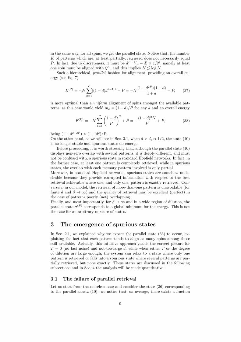
The expressions for arbitrary P can be analogously calculated exactly and someexamples are shown in Fig. 1.

Figure 1: Mattis magnetizations m versus dilution d, according to the analyticalexpression derived in Sec. 3.3. Each panel refers to a different value of P , asspecified.

We expect σH to become globally stable in the region of very large dilutions(d > dH(P )); intuitively, dilution must be large enough to make magnetizationsrather close to each other in such a way that the least signalled spins cor-responding to (−,−, ...,−,+,+, ...,+) (overall (P − 1)/2 negative entries and(P + 1)/2 positive entries) are stable. This means

∑i(1− δΞ,0)sign(Ξ)ξµi /N >∑(P−1)/2

k=1 ϕk(P + 1)/(P − k), where ϕk = 2∑l[(1− d)/2]2ldP−2l(P − k)!/[l!(l−

1)!(P − k − 2l + 1)!] and P is odd. This condition is fulfilled for values of dilu-tion larger than dH(P ), which converges to 1 as P gets larger, hence, in order to

12

tackle this limit, dilution must become a function of the system size d→ d(N).In this case the network itself becomes diluted as well and different techniquesare required; this will not be discussed in this paper.

4 Stability analysis on the organization of thestates

The set of solutions for self-consistent equations (35) describes states whosestability may vary strongly. In fact, provided the network has reached them, inthe noiseless limit (of whatever kind) it would persist in those states. However,the equations do not contain any information about whether the solutions willbe stable against small perturbations, that is to say if the system will indeedreally thermalize on these states or will fall apart more or less quickly. In orderto evaluate their stability we need to check the second derivative of the free-energy [1]. More precisely, we further need to build up the so called “stabilitymatrix” A with elements

Aµν =∂2fβ(−→m)

∂mµ∂mν. (55)

Then, we evaluate and diagonalize A at a point m, representing a particularsolution of the self-consistence equations (35), in order to determine whether mis stable or not. Being {Eµ}µ=1,...,P , the set of related eigenvalues, m is stablewhenever all of them are positive.

Now, from Eq. 34 and 55, remembering that α(β, d) = −βf(β, d), we findstraightforwardly

Aµν = [1− β(1− d)]δµν + βQµν , (56)

whereQµν = 〈ξµξν tanh2(β

−→ξ · −→m)〉ξ. (57)

Of course when d = 0 we recover Aµν = (1−β)δµν + 〈ξµξν tanh2(β−→ξ ·−→m)〉ξ,

namely the result known for the standard Hopfield model.We now consider several states, known to be solutions of self-consistence

equations (35) and check their stability. In this way we will find constraints inthe region (T, d) where those states are stable and then we will build up thephase diagram.

4.1 Paramagnetic state

Let us start with the paramagnetic state, which is described by

−→m =−→0 ; (58)

this state trivially fulfills Eq. 35.By replacing this expression in Eq.s 56 and 57 we find

Aµν = δµν [1− β(1− d)]. (59)

Therefore, in this case, A is diagonal and its eigenvalues are directly Eµ =Aµµ = 1− β(1− d),∀ν ∈ [1, P ]. We can conclude the paramagnetic state existsand is stable in the region 1−β(1−d) > 0, that is (remembering that T = β−1)

PM stability ⇒ T > 1− d. (60)

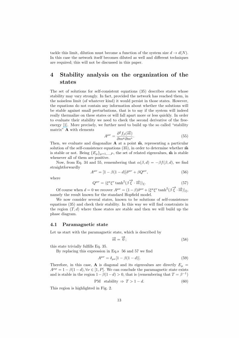
This region is highlighted in Fig. 2.

13

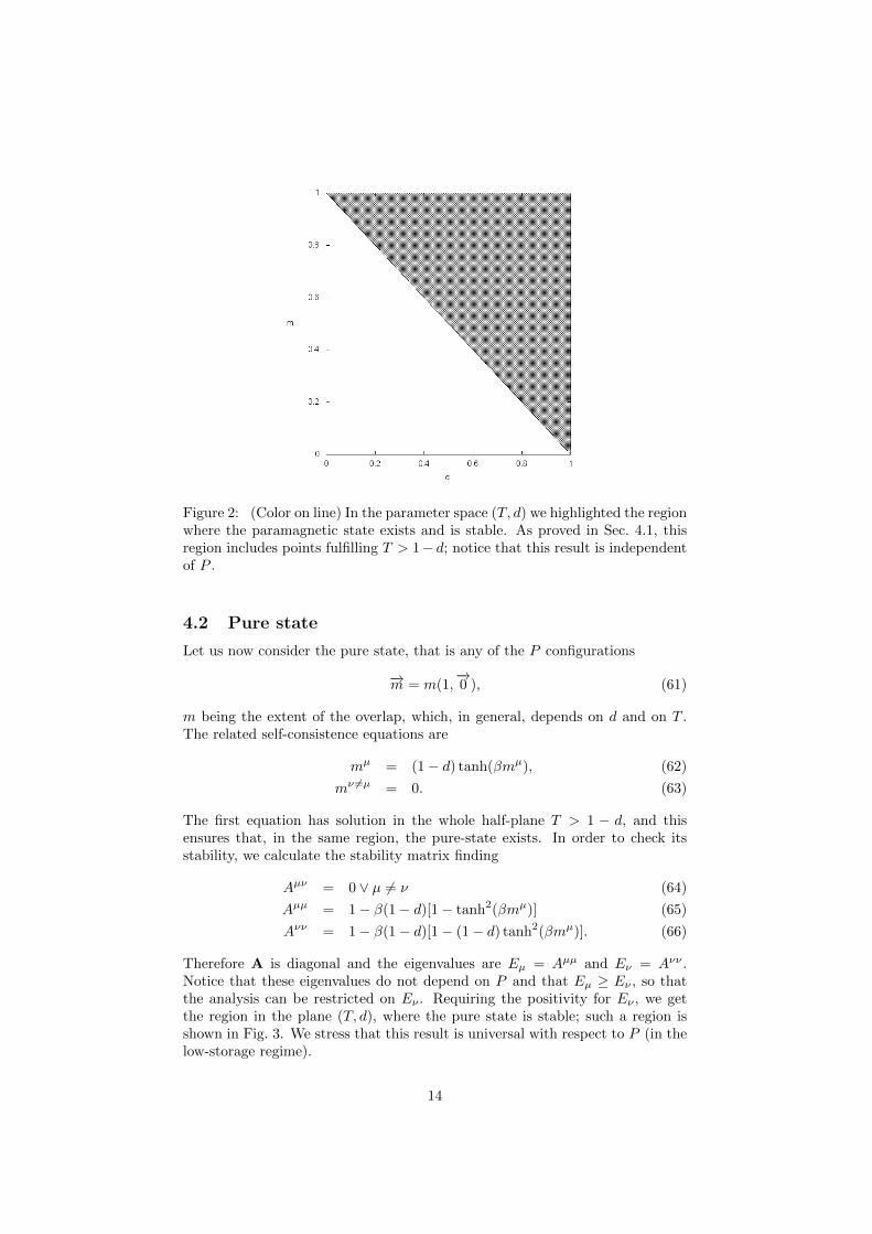
Figure 2: (Color on line) In the parameter space (T, d) we highlighted the regionwhere the paramagnetic state exists and is stable. As proved in Sec. 4.1, thisregion includes points fulfilling T > 1− d; notice that this result is independentof P .

4.2 Pure state

Let us now consider the pure state, that is any of the P configurations

−→m = m(1,−→0 ), (61)

m being the extent of the overlap, which, in general, depends on d and on T .The related self-consistence equations are

mµ = (1− d) tanh(βmµ), (62)

mν 6=µ = 0. (63)

The first equation has solution in the whole half-plane T > 1 − d, and thisensures that, in the same region, the pure-state exists. In order to check itsstability, we calculate the stability matrix finding

Aµν = 0 ∨ µ 6= ν (64)

Aµµ = 1− β(1− d)[1− tanh2(βmµ)] (65)

Aνν = 1− β(1− d)[1− (1− d) tanh2(βmµ)]. (66)

Therefore A is diagonal and the eigenvalues are Eµ = Aµµ and Eν = Aνν .Notice that these eigenvalues do not depend on P and that Eµ ≥ Eν , so thatthe analysis can be restricted on Eν . Requiring the positivity for Eν , we getthe region in the plane (T, d), where the pure state is stable; such a region isshown in Fig. 3. We stress that this result is universal with respect to P (in thelow-storage regime).

14

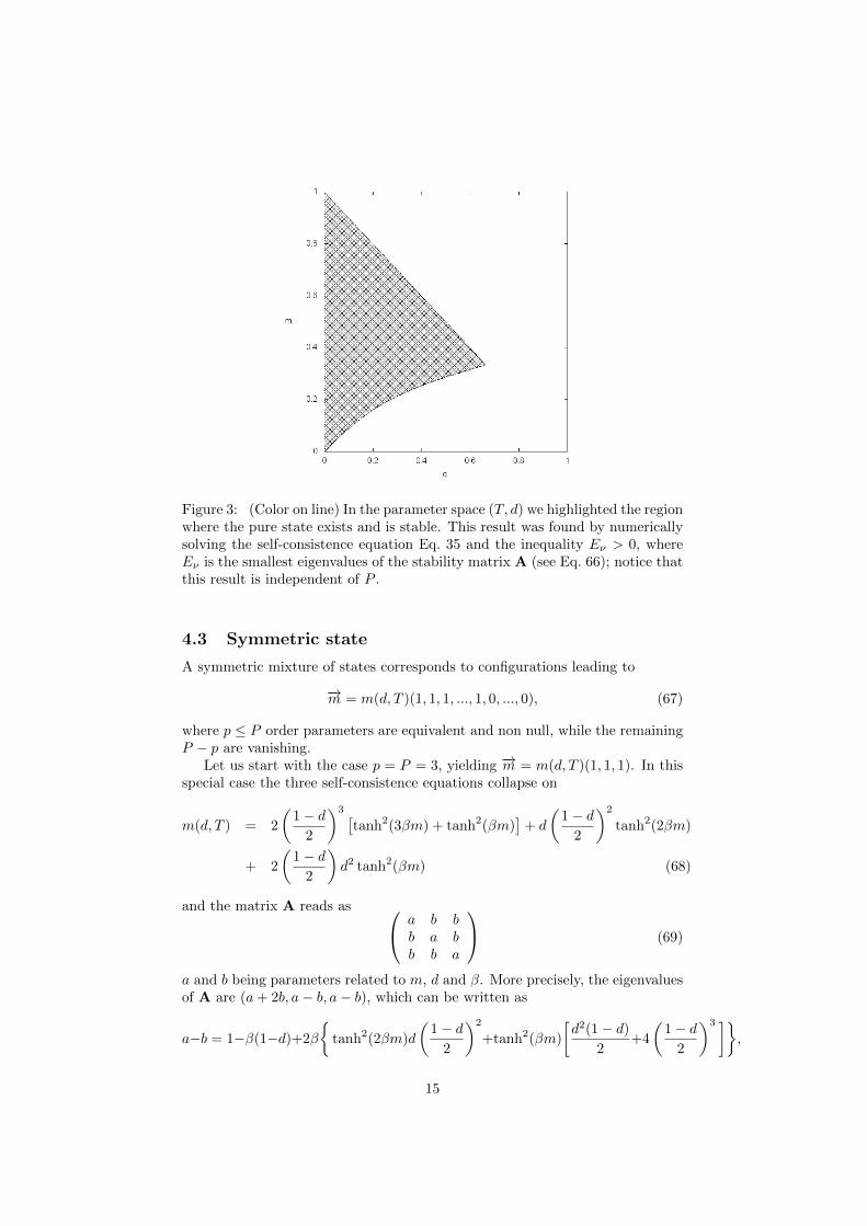
Figure 3: (Color on line) In the parameter space (T, d) we highlighted the regionwhere the pure state exists and is stable. This result was found by numericallysolving the self-consistence equation Eq. 35 and the inequality Eν > 0, whereEν is the smallest eigenvalues of the stability matrix A (see Eq. 66); notice thatthis result is independent of P .

4.3 Symmetric state

A symmetric mixture of states corresponds to configurations leading to

−→m = m(d, T )(1, 1, 1, ..., 1, 0, ..., 0), (67)

where p ≤ P order parameters are equivalent and non null, while the remainingP − p are vanishing.

Let us start with the case p = P = 3, yielding −→m = m(d, T )(1, 1, 1). In thisspecial case the three self-consistence equations collapse on

m(d, T ) = 2

(1− d

2

)3 [tanh2(3βm) + tanh2(βm)

]+ d

(1− d

2

)2

tanh2(2βm)

+ 2

(1− d

2

)d2 tanh2(βm) (68)

and the matrix A reads as a b bb a bb b a

(69)

a and b being parameters related to m, d and β. More precisely, the eigenvaluesof A are (a+ 2b, a− b, a− b), which can be written as

a−b = 1−β(1−d)+2β

{tanh2(2βm)d

(1− d

2

)2

+tanh2(βm)

[d2(1− d)

2+4

(1− d

2

)3 ]},

15

a+ 2b = 1− β(1− d) + 2β

{tanh2(3βm)3

(1− d

2

)3

+ tanh2(βm)

[d2(1− d)

2

+

(1− d

2

)3 ]}+ 8dβ tanh2(2βm)

(1− d

2

)2

. (70)

The conditions for the existance and the stability of the symmetric, odd mixturewith p = P = 3, yield a system of equations which was solved numerically andthe region were such conditions are all fulfilled is shown in Fig. 4. Notice that theregion is actually made up of two disconnected parts, each displaying peculiarfeatures, as explained later.This result is robust with respect to P , being P odd and p = P .

Figure 4: (Color on line) In the parameter space (T, d) we highlighted the regionwhere the symmetric state σ(S), for the special case p = P = 3, exists and isstable. Notice that two disconnected regions emerge: the one correspondingto lower values of dilution derives from the fact that p is odd, while the onecorresponding to larger values of dilution from the fact that p = P .

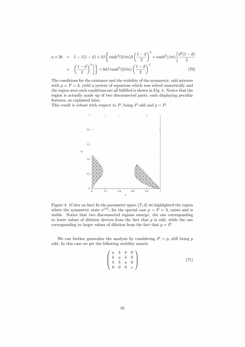
We can further generalize the analysis by considering P > p, still being podd. In this case we get the following stability matrix

a b b 0b a b 0b b a 00 0 0 c

(71)

16

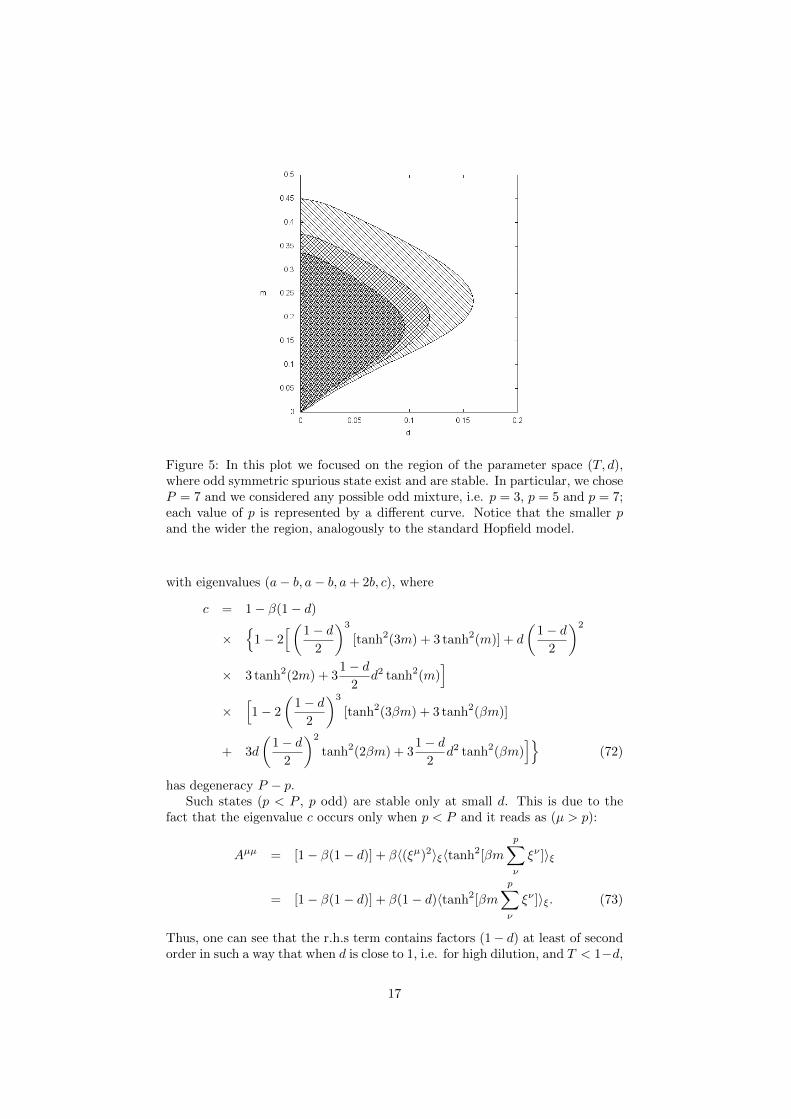
Figure 5: In this plot we focused on the region of the parameter space (T, d),where odd symmetric spurious state exist and are stable. In particular, we choseP = 7 and we considered any possible odd mixture, i.e. p = 3, p = 5 and p = 7;each value of p is represented by a different curve. Notice that the smaller pand the wider the region, analogously to the standard Hopfield model.

with eigenvalues (a− b, a− b, a+ 2b, c), where

c = 1− β(1− d)

×{

1− 2[(1− d

2

)3

[tanh2(3m) + 3 tanh2(m)] + d

(1− d

2

)2

× 3 tanh2(2m) + 31− d

2d2 tanh2(m)

]×

[1− 2

(1− d

2

)3

[tanh2(3βm) + 3 tanh2(βm)]

+ 3d

(1− d

2

)2

tanh2(2βm) + 31− d

2d2 tanh2(βm)

]}(72)

has degeneracy P − p.Such states (p < P , p odd) are stable only at small d. This is due to the

fact that the eigenvalue c occurs only when p < P and it reads as (µ > p):

Aµµ = [1− β(1− d)] + β〈(ξµ)2〉ξ〈tanh2[βm

p∑ν

ξν ]〉ξ

= [1− β(1− d)] + β(1− d)〈tanh2[βm

p∑ν

ξν ]〉ξ. (73)

Thus, one can see that the r.h.s term contains factors (1− d) at least of secondorder in such a way that when d is close to 1, i.e. for high dilution, and T < 1−d,

17

such term becomes negative. On the other hand, in the case µ ≤ p, we get

Aµµ = [1− β(1− d)] + β〈(ξµ)2 tanh2[βm

p∑ν=1

ξν ]〉ξ

and therefore the r.h.s term contains even first order term (1 − d), which arecomparable with β(1− d).

Moreover, we find that the p-component, odd symmetric state exists andis stable in a region of the space (T, d), which gets smaller and smaller as pgrows (see Fig. 5). The emergence of such states can be seen as a feature ofrobustness of the standard Hopfield model with respect to dilution.

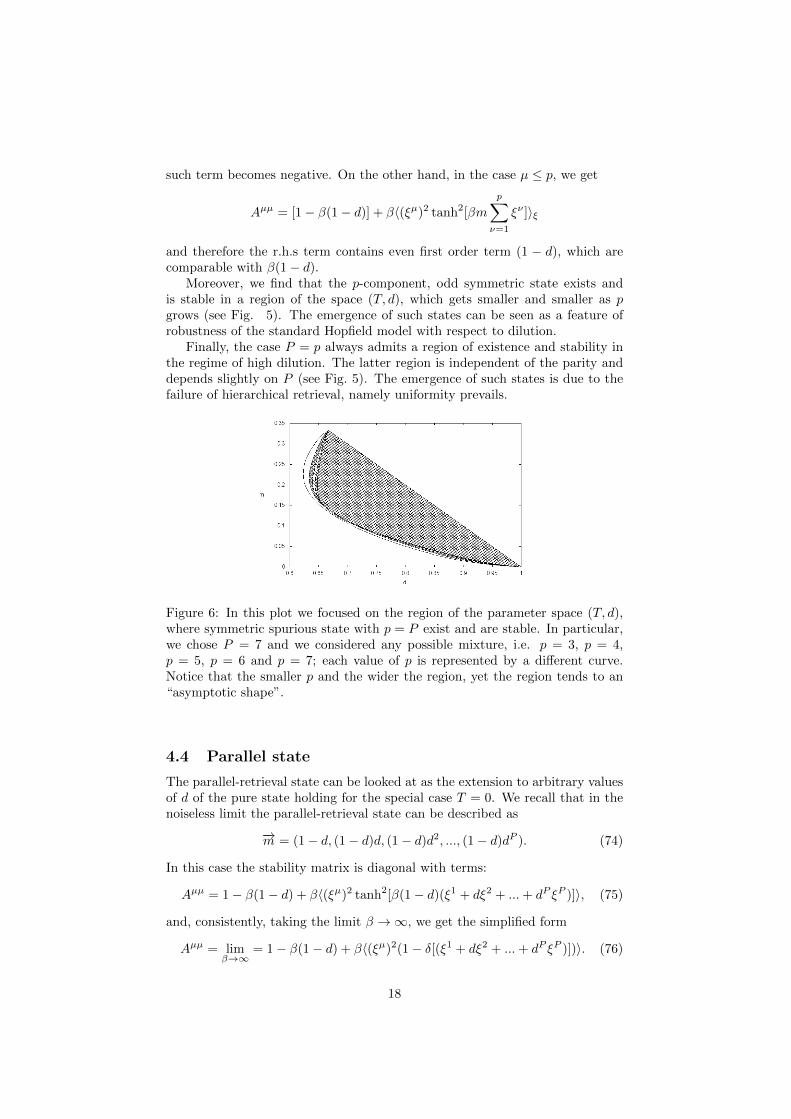
Finally, the case P = p always admits a region of existence and stability inthe regime of high dilution. The latter region is independent of the parity anddepends slightly on P (see Fig. 5). The emergence of such states is due to thefailure of hierarchical retrieval, namely uniformity prevails.

Figure 6: In this plot we focused on the region of the parameter space (T, d),where symmetric spurious state with p = P exist and are stable. In particular,we chose P = 7 and we considered any possible mixture, i.e. p = 3, p = 4,p = 5, p = 6 and p = 7; each value of p is represented by a different curve.Notice that the smaller p and the wider the region, yet the region tends to an“asymptotic shape”.

4.4 Parallel state

The parallel-retrieval state can be looked at as the extension to arbitrary valuesof d of the pure state holding for the special case T = 0. We recall that in thenoiseless limit the parallel-retrieval state can be described as

−→m = (1− d, (1− d)d, (1− d)d2, ..., (1− d)dP ). (74)

In this case the stability matrix is diagonal with terms:

Aµµ = 1− β(1− d) + β〈(ξµ)2 tanh2[β(1− d)(ξ1 + dξ2 + ...+ dP ξP )]〉, (75)

and, consistently, taking the limit β →∞, we get the simplified form

Aµµ = limβ→∞

= 1− β(1− d) + β〈(ξµ)2(1− δ[(ξ1 + dξ2 + ...+ dP ξP )])〉. (76)

18

Now, the third term in the r.h.s. is either β〈(ξµ)2〉 = β(1 − d) (when thepolynomial of order P is zero) or 0; the latter case would trivially yield Aµµ < 0.Therefore, in the limit β → ∞ the stability of the parallel-retrieval state isconstrained by the smallest real root ∈ [0, 1] of the polynomial ξ1+dξ2+...+dP ξP

with ξi = 1, 0,−1. This corresponds to ξ1 = 1 and ξi = −1,∀i > 1, under gaugesymmetry and returns the same result found, from a more empirical point ofview, in Sec. 3.1. More precisely, the critical dilution converges exponentiallyto 1/2 as P grows.

In particular, for P = 3 we find that the parallel-retrieval state exists and

is stable in the interval d ∈ (0,√

5−12 ) ' (0, 0.618). The point dc(3) =

√5−12

corresponds to the unique real root in (0, 1).When noise is introduced, the critical dilution dc, separating the parallel-

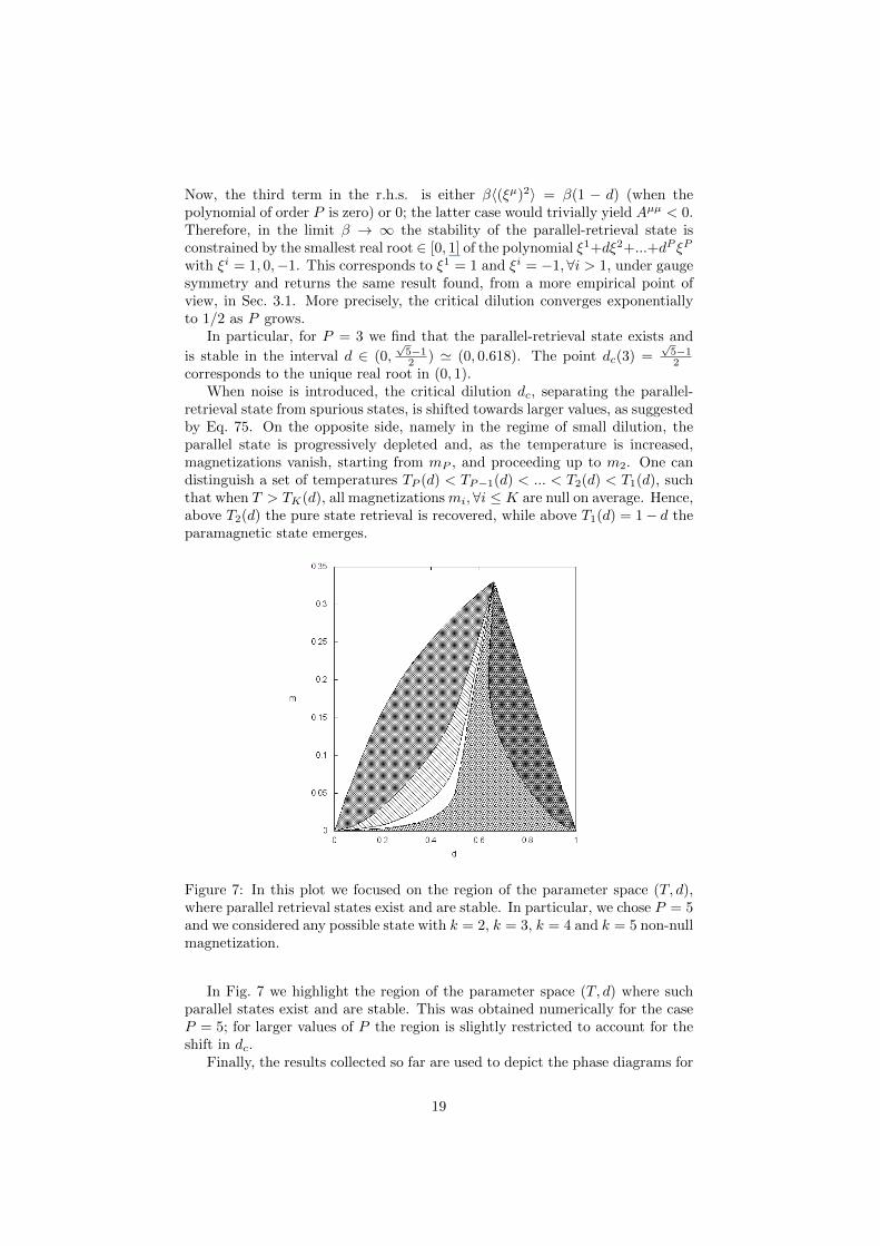
retrieval state from spurious states, is shifted towards larger values, as suggestedby Eq. 75. On the opposite side, namely in the regime of small dilution, theparallel state is progressively depleted and, as the temperature is increased,magnetizations vanish, starting from mP , and proceeding up to m2. One candistinguish a set of temperatures TP (d) < TP−1(d) < ... < T2(d) < T1(d), suchthat when T > TK(d), all magnetizationsmi,∀i ≤ K are null on average. Hence,above T2(d) the pure state retrieval is recovered, while above T1(d) = 1− d theparamagnetic state emerges.

Figure 7: In this plot we focused on the region of the parameter space (T, d),where parallel retrieval states exist and are stable. In particular, we chose P = 5and we considered any possible state with k = 2, k = 3, k = 4 and k = 5 non-nullmagnetization.

In Fig. 7 we highlight the region of the parameter space (T, d) where suchparallel states exist and are stable. This was obtained numerically for the caseP = 5; for larger values of P the region is slightly restricted to account for theshift in dc.

Finally, the results collected so far are used to depict the phase diagrams for

19

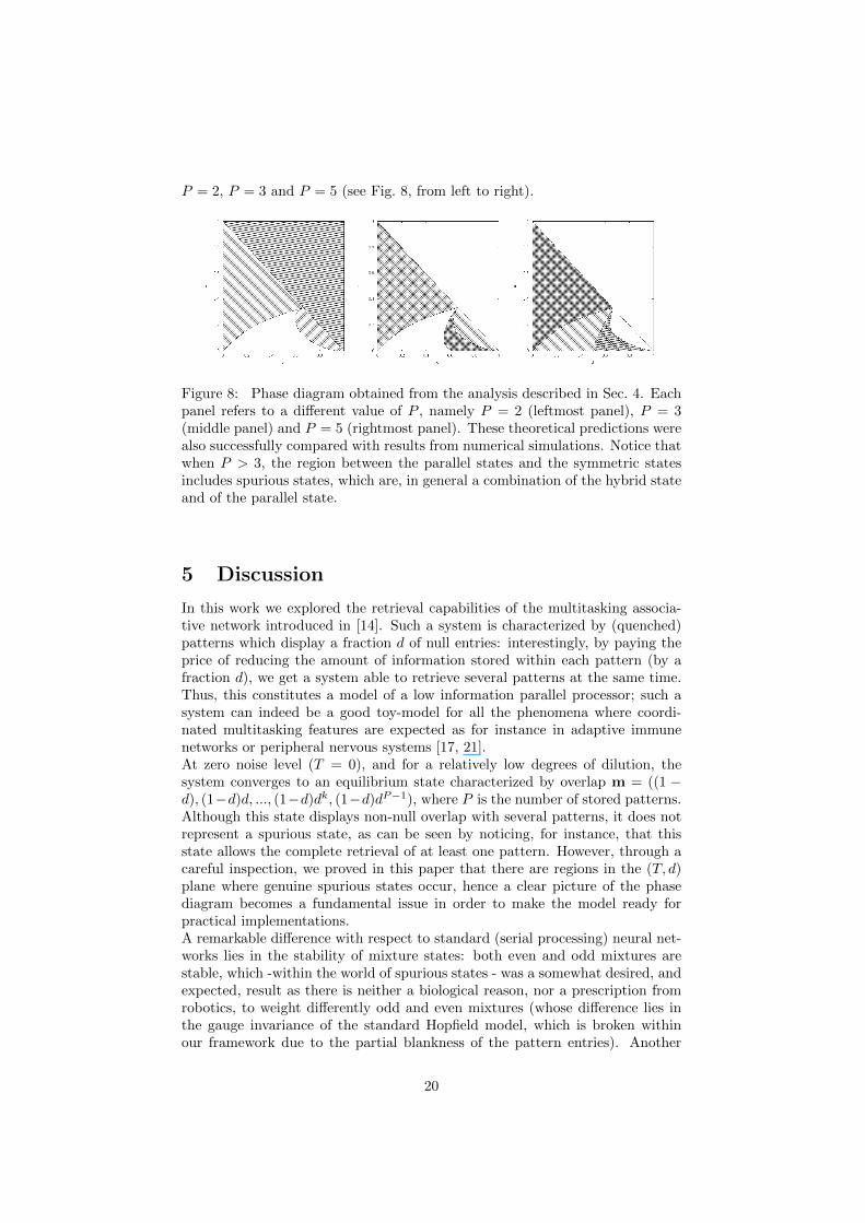
P = 2, P = 3 and P = 5 (see Fig. 8, from left to right).

Figure 8: Phase diagram obtained from the analysis described in Sec. 4. Eachpanel refers to a different value of P , namely P = 2 (leftmost panel), P = 3(middle panel) and P = 5 (rightmost panel). These theoretical predictions werealso successfully compared with results from numerical simulations. Notice thatwhen P > 3, the region between the parallel states and the symmetric statesincludes spurious states, which are, in general a combination of the hybrid stateand of the parallel state.

5 Discussion

In this work we explored the retrieval capabilities of the multitasking associa-tive network introduced in [14]. Such a system is characterized by (quenched)patterns which display a fraction d of null entries: interestingly, by paying theprice of reducing the amount of information stored within each pattern (by afraction d), we get a system able to retrieve several patterns at the same time.Thus, this constitutes a model of a low information parallel processor; such asystem can indeed be a good toy-model for all the phenomena where coordi-nated multitasking features are expected as for instance in adaptive immunenetworks or peripheral nervous systems [17, 21].At zero noise level (T = 0), and for a relatively low degrees of dilution, thesystem converges to an equilibrium state characterized by overlap m = ((1 −d), (1−d)d, ..., (1−d)dk, (1−d)dP−1), where P is the number of stored patterns.Although this state displays non-null overlap with several patterns, it does notrepresent a spurious state, as can be seen by noticing, for instance, that thisstate allows the complete retrieval of at least one pattern. However, through acareful inspection, we proved in this paper that there are regions in the (T, d)plane where genuine spurious states occur, hence a clear picture of the phasediagram becomes a fundamental issue in order to make the model ready forpractical implementations.A remarkable difference with respect to standard (serial processing) neural net-works lies in the stability of mixture states: both even and odd mixtures arestable, which -within the world of spurious states - was a somewhat desired, andexpected, result as there is neither a biological reason, nor a prescription fromrobotics, to weight differently odd and even mixtures (whose difference lies inthe gauge invariance of the standard Hopfield model, which is broken withinour framework due to the partial blankness of the pattern entries). Another

20

expected feature, which we confirmed in this paper, is the emergence of parallelspurious states beyond standard ones from classical neural network theory: Thisis the natural generalization of the latter when moving from serial to parallelprocessing.

Beyond these somehow attended results, the phase diagram of the model isstill very rich and composed by several not-overlapping regions where the re-trieval states are deeply differently structured: Beyond the paramagnetic stateand the pure state, the system is able to achieve both a hierarchical organiza-tion of pattern retrievals (for intermediate values of dilution) and a completelysymmetric parallel state (for high values of dilution), which act as the basis forthe outlined mixtures when raising the noise level above thresholds whose valuedepends on the load of the network P .These findings have been obtained developing a new strategy for computing thefree energy of the model by which, imposing thermodynamic principles (henceextremizing the latter over the order parameters of the model), self-consistencyhas been obtained. The whole procedure has been strongly based on techniquesstemmed from partial differential equation theory. In particular, the key ideais showing that the noise-derivatives of the statistical pressure obey Burgers’equations, which can be solved through the Cole-Hopf transformation. The lat-ter maps the evolution of the free energy over the noise into a diffusion problemwhich can be addressed through standard Green integration in momenta spaceand then pushed back in the original framework.In the future, effort must still be spent in order to achieve a clear scenario inthe hyper-diluted regime, namely where the dilution scales as a function of thevolume (the amount of neurons), which can not be accomplished through thetechniques we presented here as saddle point integration is no longer useful. Weplan to report on this research soon.

This work is supported by FIRB grant RBFR08EKEV.Sapienza Universita’ di Roma and INFN are acknowledged too for partial finan-cial support.

References

[1] D. Amit. Modeling Brain Function. Cambridge University Press, 1989.

[2] D.J. Amit, H. Gutfreund, and H. Sompolinsky. Storing infinite numbers ofpatterns in a spin-glass model of neural networks. Physical Review Letters,55:1530–1533, 1985.

[3] M. Mezard, G. Parisi, and M. A. Virasoro. Spin glass theory and beyond.World Scientific, Singapore, 1987.

[4] J.J. Hopfield. Neural networks and physical systems with emergent col-lective computational abilities. Proc. Natl. Acad. Sc. USA, 79:2554–2558,1982.

[5] B. Cheng and D. M. Titterington. Neural networks: A review from astatistical perspective. Statistical Science, 9(1):2–30, 1994.

21

[6] S. Nolfi and D. Floreano. Evolutionary robotics: The biology, intelligence,and technology of self-organizing machines. 2000.

[7] R.R. Trippi and E. Turban. Neural Networks in Finance and Investing:Using Artificial Intelligence to Improve Real World Performance. McGraw-Hill, Inc. New York, NY, USA, 1992.

[8] E. Agliari, A. Barra, F. Guerra, and F. Moauro. A thermodynamic per-spective of immune capabilities. J. Theor. Biol., 287:48–63, 2011.

[9] H. Sompolinsky. Neural networks with non-linear synapses and a staticnoise. Physical Review A, 34:2571, 1986.

[10] T. Nikoletopoulos, A.C.C. Coolen, I. Perez-Castillo, N.S. Skantzos, J.P.L.Hatchett, and B Wemmenhove. Replicated transfer matrix analysis of isingspin models on ’small world’ lattices. Journal of Physics A: Mathematicaland General, 37:6455, 2004.

[11] B. Wemmenhove and A.C.C. Coolen. Finite connectivity attractor neuralnetworks. Journal of Physics A Mathematical and Theoretical, 36(9617),2003.

[12] A. Barra, F. Guerra, and G. Genovese. The replica symmetric approx-imation of the analogical neural network. Journal of Statistical Physics,140(4):784, 2010.

[13] A. Barra, A. Bernacchia, E. Santucci, and P. Contucci. On the equivalenceof hopfield networks and boltzmann machines. Neural Networks, 2012.

[14] E. Agliari, A. Barra, A. Galluzzi, F. Guerra, and F. Moauro. MultitaskingAssociative Networks. Physical Review Letters, 109:268101, 2012.

[15] E. Agliari, A. Barra, A. De Antoni, and A. Galluzzi. Parallel retrievalof correlated patterns: From Hopfield networks to Boltzmann machines.Neural Networks, 38:52–63, 2012.

[16] A.C.C. Coolen, R. Kuhn, and P. Sollich. Theory of Neural InformationProcessing Systems. Oxford University Press, 2005.

[17] E. Agliari, A. Barra, S. Bartolucci, A. Galluzzi, F. Guerra, and F. Moauro.Parallel processing in immune networks. submitted, 2012.

[18] D.J. Willshaw and C. von der Malsburg. How patterned neural connectionscan be set up by self-organization. Proc. R. Soc. Lond. B, 194:431–445,1976.

[19] A. Barra, A. Di Biasio, and F. Guerra. Replica symmetry breaking inmean-field spin glasses through the hamilton–jacobi technique. Journal ofStatistical Mechanics: Theory and Experiment, 2010:P09006, 2010.

[20] G. Genovese and A. Barra. A mechanical approach to mean field models.Journal of Mathematical Physics, 50:053303, 2009.

[21] E. Agliari, A. Annibale, A. Barra, A.C.C. Coolen, and D. Tantari. Immunenetworks: Multitasking properties at medium load. submitted, 2013.

22