Multistable solitons in higher-dimensional cubic–quintic nonlinear Schrödinger lattices

arX

iv:0

804.

0497

v1 [

nlin

.PS]

3 A

pr 2

008

Multistable Solitons in Higher-Dimensional Cubic-Quintic Nonlinear

Schrodinger Lattices

C. Chong a,∗ , R. Carretero-Gonzalez b, B.A. Malomed c, and P.G. Kevrekidis d

aInstitut fur Analysis, Dynamik und Modellierung, Universitat Stuttgart, Stuttgart 70178, GermanybNonlinear Dynamical Systems Group1, Computational Sciences Research Center, and

Department of Mathematics and Statistics, San Diego State University, San Diego, CA 92182-7720, USAcDepartment of Interdisciplinary Studies, Faculty of Engineering, Tel Aviv University, Tel Aviv 69978, Israel

dDepartment of Mathematics and Statistics, University of Massachusetts, Amherst MA 01003-4515, USA

Abstract

We study the existence, stability, and mobility of fundamental discrete solitons in two- and three-dimensional nonlinear Schrodingerlattices with a combination of cubic self-focusing and quintic self-defocusing onsite nonlinearities. Several species of stationarysolutions are constructed, and bifurcations linking their families are investigated using parameter continuation starting from theanti-continuum limit, and also with the help of a variational approximation. In particular, a species of hybrid solitons, intermediatebetween the site- and bond-centered types of the localized states (with no counterpart in the 1D model), is analyzed in 2D and3D lattices. We also discuss the mobility of multi-dimensional discrete solitons that can be set in motion by lending them kineticenergy exceeding the appropriately crafted Peierls-Nabarro barrier; however, they eventually come to a halt, due to radiation loss.

Key words: Nonlinear Schrodinger equation; solitons; bifurcations; nonlinear lattices; higher-dimensionalPACS: 52.35.Mw, 42.65.-k, 05.45.a, 52.35.Sb

1. Introduction

A large number of models relevant to various fields ofphysics is based on discrete nonlinear Schrodinger (DNLS)equations [1]. A realization of the one-dimensional (1D)DNLS model in arrays of parallel optical waveguides waspredicted in Ref. [2], and later demonstrated experimen-tally, using an array mounted on a common substrate [3].Multi-channel waveguiding systems can also be created asphotonic lattices in bulk photorefractive crystals [4]. Dis-crete solitons are fundamental self-supporting modes in theDNLS system [1]. The mobility [5,6] and collisions [6,7] ofdiscrete solitons have been studied in 1D systems of theDNLS type with the simplest self-focusing cubic (Kerr)nonlinearity. The DNLS equation with the cubic onsite non-linearity is also a relevant model for the Bose-Einstein con-densate (BEC) trapped in deep optical lattices [8].

∗ Corresponding authorURL:

http://www.iadm.uni-stuttgart.de/LstAnaMod/Chong/home.html

(C. Chong).1 URL: http://nlds.sdsu.edu/

A more general discrete cubic nonlinearity appears in theSalerno model [9], which combines the onsite cubic termsand nonlinear coupling between adjacent sites. A modifi-cation of the Salerno model, with opposite signs in front ofthe onsite and inter-site cubic terms, makes it possible tostudy the competition between self-focusing and defocus-ing discrete nonlinearities. This has been done in both 1D[10] and 2D [11] settings.

Lattice models with saturable onsite nonlinear termshave been studied too. The first model of that type was in-troduced by Vinetskii and Kukhtarev in 1975 [12]. Brightsolitons in this model were predicted in 1D [13] and 2D [14]geometries. Lattice solitons supported by saturable self-defocusing nonlinearity were created in an experiment con-ducted in an array of optical waveguides built in a photo-voltaic medium [15]. Dark discrete solitons were also con-sidered experimentally [16] and theoretically [17] in the lat-ter model.

The experimental observation of optical nonlinearitiesthat may be fitted by a combination of self-focusing cu-bic and self-defocusing quintic terms [18] suggests to studythe dynamics of solitons in the NLS equation with cubic-quintic (CQ) nonlinearity. A family of stable exact soliton

Preprint submitted to Physica D 3 April 2008

solutions to the 1D continuum NLS equation of this type iswell known [19]. The possibility to build an array of parallelwaveguides using optical materials with the CQ nonlinear-ity lends relevance to the consideration of the DNLS equa-tion with the onsite nonlinearity of the CQ type. In particu-lar, this DNLS equation arises as a limit case of the contin-uum CQ-NLS equation which includes a periodic potentialin the form of periodic array of rectangular channels, i.e.,the Kronig-Penney lattice. Families of stable bright soli-tons were found in 1D [20] and 2D [21] versions of the lattermodel (the latter one with a “checkerboard” 2D potentialsupports both fundamental and vortical solitons).

The findings of a CQ-DNLS model may also be relevantto the case of a self-attractive BECs confined in a 2D planeby a “pancake”-shaped trap combined with a sufficientlystrong 2D optical-lattice potential (although quantum ef-fects such as a superfluid to Mott insulator transition arealso relevant in the latter [22]). The condensate trapped ineach individual potential well of this configuration is de-scribed by the Gross-Pitaevskii equation with an extra self-attractive quintic term which accounts for the deviation ofthe well’s shape from one-dimensionality [23]. The tunnel-ing of atoms between adjacent potential wells in this set-ting is approximated by the linear coupling between sitesof the respective lattice.

The simplest stationary bright solitons, of the unstag-

gered type (without spatial oscillations in the solitons’tails), have been studied in the 1D version of the CQ-DNLSmodel in Ref. [24]. It was demonstrated that this classof solitons includes infinitely many families with distinctsymmetries. The stability of the basic families was ana-lyzed, and bifurcations between them were explored in anumerical form, and by means of a variational approxima-tion (VA). Dark solitons in the same model were recentlystudied [25] and, in another very recent work, staggered1D bright solitons as well as the mobility of unstaggeredones have been investigated [26].

The aim of the present work is to study the existence,stability, and mobility of bright discrete solitons in two-and three-dimensional (2D and 3D) NLS lattices with thenonlinearity of the CQ type. As suggested by the previ-ous works, especially Ref. [24], the competition of the self-focusing cubic and self-defocusing quintic nonlinearities inthe setting of the discrete model may readily give rise tomulti-stability of discrete solitons, which is not possible inthe ordinary cubic DNLS model [27], nor in the discrete CQmodel where both nonlinear terms are self-focusing [28]. Inaddition to that, one may expect that the CQ model sharesmany features with those including saturable nonlinearity[29,14], such as enhanced mobility of multidimensional dis-crete solitons (as mentioned above, mobile discrete solitonscan be readily found in the 1D CQ-DNLS equation [26]).

The paper is organized as follows: in the next section,we introduce the model and outline the method used toconstruct the multi-dimensional discrete solitons. In Sec. 3,we focus on stability and existence regions for 2D discretesolitons, and the respective bifurcations. Mobility of the 2D

solitons on the lattice is studied in Sec. 4. Section 5 reportsextensions of these results to 3D latices. In Sec. 6 we reportanalytical results obtained by means of a VA, and Sec. 7concludes the paper.

2. The model

In dimensionless form, the 2D DNLS equation with theonsite nonlinearity of the CQ type has the following form:

iψn,m+C∆(2)ψn,m+2|ψn,m|2ψn,m−|ψn,m|4ψn,m = 0, (1)

where ψn,m is the complex field at site {n,m} (the ampli-tude of the electromagnetic field in an optical fiber, or localmean-field wave function in BEC), ψ ≡ dψ/dt, and C > 0is the coupling constant of the lattice model. We assume anisotropic medium, hence the discrete Laplacian is taken as

∆(2)ψn,m ≡ ψn+1,m +ψn−1,m +ψn,m+1 +ψn,m−1−4ψn,m.(2)

The CQ nonlinearity is represented by the last two termsin Eq. (1).

Equation (1) conserves two dynamical invariants: norm(or power, in terms of optics),

M =∑

n,m

|ψn,m|2, (3)

and energy (Hamiltonian),

H =∑

n,m

[

C(|ψn+1,m − ψn,m|2 + |ψn,m+1 − ψn,m|2)

−|ψn,m|4 +1

3|ψn,m|6

]

. (4)

The conserved quantities play an important role in the anal-ysis of the mobility of discrete solitons, see Sec. 4 below.

Steady state solutions are sought for in the usual form,ψn,m = un,m exp(−iµt), where µ is the real frequency, andthe real stationary lattice field un,m satisfies the followingdiscrete equation:

µun,m + C∆(2)un,m + 2u3n,m − u5

n,m = 0. (5)

More general solutions carrying topological charge, forwhich stationary field un,m is complex, fall outside of thescope of the present work, and will be considered elsewhere.

In one dimension, bright-soliton solutions of Eq. (5) canbe found as homoclinic orbits of the corresponding two-dimensional discrete map [30]. This technique was used toconstruct 1D soliton solutions to the CQ-DNLS model inRef. [24]. Since this method is not available in higher di-mensions, we construct the solutions starting from the anti-continuum limit, C → 0, and perform parameter continu-ation to C > 0. A multidimensional version of the VA canalso be used to construct solutions for small values of C,see Sec. 6 below.

In Ref. [24], two fundamental types of solutions werestudied: site-centered and bond-centered solitons. Each

2

−5 0 5

0

0.5

1

u n

−5 0 5

0

0.5

1

−5 0 5

0

0.5

1

u n

n−5 0 5

0

0.5

1

n

Fig. 1. (Color online) Solutions to Eq. (1) for (µ, C) = (−0.7, 0),which are used as seeds to find nontrivial solutions at C > 0 (only a1D slice is shown, see Fig. 3 for profiles in two dimensions). Top left:“Tall” (blue cross markers) and “short” (red plus markers) site-cen-tered solutions. Top right: “Tall” and “short” bond-centered solu-tions. Bottom: wider extensions of the “tall” site-centered solution.

−5 0 5

0

0.5

1

u n

−5 0 5

0

0.5

1

−5 0 5

0

0.5

1

u n

n−5 0 5

0

0.5

1

n

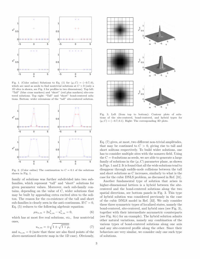
Fig. 2. (Color online) The continuation to C = 0.1 of the solutionsshown in Fig. 1.

family of solutions was further subdivided into two sub-families, which represent “tall” and “short” solutions forgiven parameter values. Moreover, each sub-family con-tains, depending on the value of C, wider solutions thatmay be built by appending extra excited sites to the soli-ton. The reason for the co-existence of the tall and shortsub-families is clearly seen in the anti-continuum. If C = 0,Eq. (5) reduces to the following algebraic equation:

µun,m + 2u3n,m − u5

n,m = 0, (6)

which has at most five real solutions, viz., four nontrivialones,

un,m = ±

√

1 ±√

1 + µ, (7)

and un,m = 0 (note that these are also fixed points of theabove-mentioned discrete map in the 1D case). Obviously,

−50

5

−50

50

0.5

1

nm

u n,m

−50

5

−50

50

0.5

1

nm

u n,m

−50

5

−50

50

0.5

1

nm

u n,m

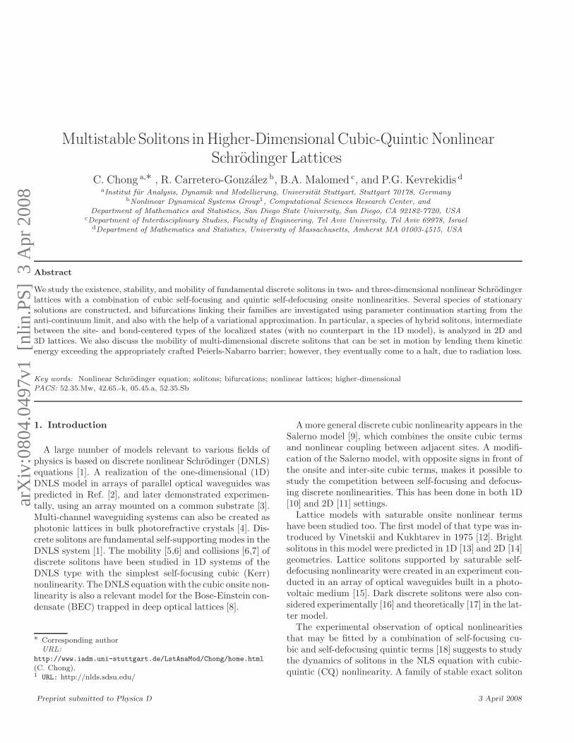
Fig. 3. Left (from top to bottom): Contour plots of solu-tions of the site-centered, bond-centered, and hybrid types for(µ, C) = (−0.7, 0.1). Right: The corresponding 3D plots.

Eq. (7) gives, at most, two different non-trivial amplitudes,that may be continued to C > 0, giving rise to tall andshort solitons respectively. To build wider solutions, onehas to consider multiple sites with the nonzero field. Usingthe C = 0 solutions as seeds, we are able to generate a largefamily of solutions in the (µ,C) parameter plane, as shownin Figs. 1 and 2. It is found that all the wide solutions tend todisappear through saddle-node collisions between the talland short solutions as C increases, similarly to what is thecase for the cubic DNLS problem, as discussed in Ref. [31].

Another fundamental type of solution that arises inhigher-dimensional lattices is a hybrid between the site-centered and the bond-centered solutions along the twospatial directions, see bottom panels in Fig. 3. This typeof hybrid solution was considered previously in the caseof the cubic DNLS model in Ref. [32]. We only considerthese three symmetric types of localized states, namely thebond-centered, site-centered, and hybrid ones (see Fig. 3),together with their intermediate asymmetric counterparts(see Fig. 8(c) for an example). The hybrid solution admitsother natural variations, namely any combination of thevarious types of bond-centered solutions along one axisand any site-centered profile along the other. Since theirbehaviors are very similar, we consider only one such typeof solutions.

3

−1 −0.8 −0.6 −0.4 −0.2 00

2

4

6

8

10

µ

M

(a)

−50

5

−50

50

0.5

1

−50

5

−50

50

0.5

1

−50

5

−50

50

0.5

1

−50

5

−50

50

0.5

1

−50

5

−50

50

0.5

1

−50

5

−50

50

0.5

1

−50

5

−50

50

0.5

1

−50

5

−50

50

0.5

1

−1 −0.8 −0.6 −0.4 −0.2 00

2

4

6

8

10

µ

M

(b)

−1 −0.8 −0.6 −0.4 −0.2 00

2

4

6

8

10

µ

M

(c)

−1 −0.8 −0.6 −0.4 −0.2 00

10

20

30

40

50

60

70

µ

M

(d)

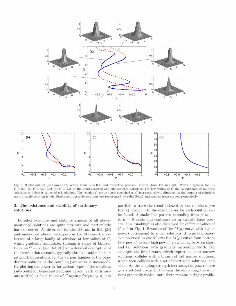
Fig. 4. (Color online) (a) Power (M) versus µ for C = 0.1, and respective profiles. Bottom (from left to right): Power diagrams, for (b)C = 0.3, (c) C = 0.4, and (d) C = 2.0, of the bond-centered and site-centered solutions. For low values of C the co-existence of multiplesolutions at different values of µ is obvious. The “snaking” pattern gets stretched as C increases, slowly diminishing the number of solutionsuntil a single solution is left. Stable and unstable solutions are represented by solid (blue) and dashed (red) curves, respectively.

3. The existence and stability of stationary

solutions

Detailed existence and stability regions of all above-mentioned solutions are quite intricate and particularlyhard to detect. As described for the 1D case in Ref. [24]and mentioned above, we expect in the 2D case the ex-istence of a large family of solutions at low values of C,which gradually annihilate, through a series of bifurca-tions, as C → ∞ (see Ref. [31] for a detailed description ofthe termination scenaria, typically through saddle-node orpitchfork bifurcations, for the various families of the basicdiscrete solitons as the coupling parameter is increased).By plotting the power M for various types of the solutions(site-centered, bond-centered, and hybrid, each with vari-ous widths) at fixed values of C against frequency µ, it is

possible to trace the trend followed by the solutions (seeFig. 4). For C = 0, the exact power for each solution canbe found. A snake like pattern extending from µ = −1to µ = 0 exists and continues for arbitrarily large pow-ers. This “snaking” is also displayed for different values ofC > 0 in Fig. 4. Branches of the M(µ) curve with higherpowers correspond to wider solutions. A typical progres-sion observed as one follows the M(µ) curve from bottom(low power) to top (high power) is switching between shortand tall solutions with gradually increasing width. Forexample, the first branch, which represents short narrowsolutions, collides with a branch of tall narrow solutions,which then collides with a set of short wide solutions, andso on. As the coupling strength increases, the power curvegets stretched upward. Following the stretching, the solu-tions gradually vanish, until there remains a single profile.

4

−0.5 −0.4 −0.3 −0.2 −0.12

4

6

8

10

µ

M

Site−centered

Bond−centered

Asymmetric

−0.32 −0.3 −0.28 −0.26 −0.24 −0.223.2

3.4

3.6

3.8

4

4.2

4.4

µ

M

Site−centered

Bond−centered

Asymmetric

Fig. 5. (Color online) Top: Pitchfork bifurcations of the bond-cen-tered solutions and site-centered solutions for lattice coupling con-stant C = 0.5. Hybrid solutions are omitted here for clarity. Bottom:Zoom of the bifurcation scenario depicted by the rectangular regionin the top panel.

Similar to what was found in cubic DNLS equation inRef. [33] the bright stationary solutions in the CQ modelalso bifurcate from plane waves (near µ ≈ 0 for the CQmodel). It is worthwhile to highlight here the increasedlevel of complexity of the relevant M(µ) curves in thecubic-quintic model (due to the interplay of short and tallsolution branches) in comparison to its cubic counterpartof Ref. [32], which features a single change of monotonicity(and correspondingly of stability) between narrow and tall(stable) and wide and short (unstable) solutions.

Reference [33] provides heuristic arguments for the exis-tence of energy thresholds for a large class of discrete sys-tems with dimension higher than some critical value. Thisclaim was proved in Ref. [34] for DNLS models with thenonlinearities of the form |ψn|

2σ+1ψn and for chains of NLSequations. As can be discerned in Fig. 4, such thresholdsalso exist in the case of the cubic-quintic nonlinearity.

In Ref. [24] a stability diagram for the discrete solitons inthe 1D model was presented in the (µ,C) plane, which gavea clear overview of the situation. However, in the presentsituation, the M(µ) curves for various fixed values of C,such as those displayed in Fig. 4, provide for a better under-standing of relationships between different solutions. Forexample, in the (µ,C) diagram, it would appear that thetaller solutions cease to exist at (µ,C) ≈ (−0.6, 0.4). How-ever, the respective M(µ) curve shows that narrow and

−0.42 −0.4 −0.38 −0.36 −0.34 −0.32 −0.3 −0.282.5

3

3.5

4

4.5

5

µ

M

Bond−centered

Asymmetric

Site−centered

Hybrid

Asymmetric

a b

c

d

Fig. 6. (Color online) Bifurcations for C = 0.4 showing that all threefundamental modes (site-centered, bond-centered, and hybrid) areall connected to each other via stability exchange with asymmetricsolutions. Two asymmetric solutions are created where the bond–centered solution loses stability at the bifurcation point labeled by‘a’ in the diagram. One of these asymmetric solutions is connectedto the hybrid solution at ‘b’ and the other is connected to the site–centered solution at point ‘c’. A third type of asymmetric solutionalso emanates from the bifurcation point ‘c’ which is connected tothe hybrid solution at ‘d’.

wide solitons become indistinguishable at this point, anddeciding which solution, short or tall, is annihilated be-comes quite arbitrary.

A numerical linear stability analysis was performed inthe usual way (see Ref. [24] for details) to investigate thestability of each of the solution branches. As one follows aM(µ) curve from bottom to top, the stability is typicallyswapped around each turning point, as seen in Fig. 4. How-ever, the stability is not switched exactly at these points,as this happens via asymmetric solutions (see below).

Similar to the 1D model, a pitchfork-like bifurcation oc-curs between the site- and bond-centered discrete solitons.This is more clearly seen in Fig. 5. For C = 0.5, the bond-centered solution loses its stability in a neighborhood of µ ≈−0.53, and asymmetric solutions are created there. Thereare multiple asymmetric solutions in this case, but only onecurve appears in Fig. 5, since each one is just a rotationof the other, hence they have the same power. The bond-centered solution loses its stability before the site-centeredsolution regains its stability; in fact, the site-centered soli-ton regains the stability exactly when the asymmetric solu-tions collide with it. This sort of stability exchange occursthroughout the M(µ) curve. The top panel of Fig. 5 showstwo such bifurcations, with a zoom of one of them shownin the bottom panel.

Figure 6 shows again a site-centered solution connectedto a bond-centered solution but also features a connectionof the site- and bond-centered solutions via the hybrid so-lution. So not only are all variations (tall, short, narrow,etc) within each mode connected, as shown by the snakelike power curves, but all the fundamental modes (bond-

5

centered, site-centered, hybrid) are also connected.We stress that the stability regions of the above men-

tioned fundamental modes are disjoint in regions wherethey each have roughly the same power and, unlike the 1Dmodel, the asymmetric solutions are unstable. These fea-tures can be seen in Figs. 5 and 6. Note that the multi-stability of symmetric solutions still occurs in this case dueto the existence of arbitrarily wide solutions at fixed valuesof C (see Fig. 4). As a general comment, it should be notedthat many of the features of the 2D cubic-quintic model(such as e.g., the existence of unstable asymmetric solu-tions, and their connecting the fundamental modes) canalso be observed in the case of the saturable model [14], al-though in the present case of the cubic-quintic model, therelevant phenomenology is even richer due to, for instance,the existence of multiple (i.e., tall and short) steady states.

4. The mobility

In one dimension, traveling solutions can be found in theform

ψn = u(n− vt)eiµt, (8)

where v is a real velocity. Substitution of this expressionin the 1D DNLS model yields the following advance-delaydifferential equation

0 =−i[vu(z) + iµu(z)] + 2|u(z)|2u(z) − |u(z)|4u(z)

+C [u(z + 1) + u(z − 1) − 2u(z)] , (9)

where z = n−vt. Stationary solutions are said to be transla-

tionally invariant if the function un = u(nh), where h is thelattice spacing, can be extended to a one-parameter fam-ily of continuous solutions, u(z − s), of the advance-delayequation (9) with v = 0. Solutions of this type have beenfound in other lattice models (see Ref. [35,36] and referencestherein). Localized solutions with non-oscillatory tails insimilar models for v 6= 0, have been found in Ref. [29,37]by solving a respective counterpart of Eq. (9). If transla-tionally invariant solutions exist, then the sundry modes(bond-centered, site-centered, etc.) are generated by thesame continuous function u(z−s), each with a correspond-ing value of s. The translationally invariant solutions occur(i) at transparency points, which are points in the parame-ter space where solutions exchange their stability, and (ii)if the Peierls-Nabarro (PN) barrier vanishes; the barrierbeing defined as the difference in energy between the site-centered and bond-centered solutions. Note that (i) and(ii) are necessary but not sufficient conditions for the ex-istence of translationally invariant solutions. For higher-dimensional lattices, translationally invariant solutions forDNLS-like models have not been found yet. However, effec-tively mobile lattice solitons have been found in 2D modelsin regions of the parameter space where the PN barrier islow (enhanced mobility). This has been the case both forquadratic nonlinearities [38] and in the vicinity of stabilityexchanges for saturable models [14]. The resulting mobile

n

t

10 20

100

200

300(a)

n10 20

(b)

n10 20

(c)

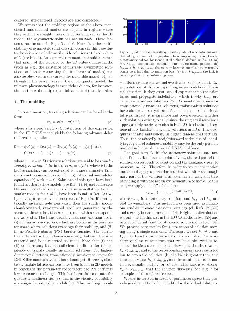
Fig. 7. (Color online) Resulting density plots, of a one-dimensionalslice along the axis of propagation, from imprinting momentum toa stationary soliton by means of the “kick” defined in Eq. 10. (a)k < kdepin: the solution remains pinned at its initial position. (b)kdepin < kn < kdisperse: the solution becomes mobile, but eventuallycomes to a halt due to radiation loss. (c) k > kdisperse: the kick isso strong that the solution disperses.

solutions radiate energy and eventually come to a halt. Ex-act solutions of the corresponding advance-delay differen-tial equation, if they exist, would experience no radiationlosses and propagate indefinitely, which is why they arecalled radiationless solutions [29]. As mentioned above fortranslationally invariant solutions, radiationless solutionshave also not been yet been found in higher-dimensionallattices. In fact, it is an important open question whethersuch solutions exist typically, since the single tail resonanceappropriately made to vanish in Ref. [29] to obtain such ex-ponentially localized traveling solutions in 1D settings, ac-quires infinite multiplicity in higher dimensional settings.Thus, the admittedly straightforward technique of identi-fying regions of enhanced mobility may be the only possiblemethod in higher dimensional DNLS problems.

The goal is to “kick” the stationary solutions into mo-tion. From a Hamiltonian point of view, the real part of thesolution corresponds to position and the imaginary part tomomentum [27]. Therefore, in order to set it into motionone should apply a perturbation that will alter the imagi-nary part of the solution in an asymmetric way, and thusproviding it with the necessary momentum to move. To thisend, we apply a “kick” of the form

un,m(0) = un,mei(knn+kmm), (10)

where un,m is a stationary solution, and kn, and km arereal wavenumbers. This method has been used in numer-ous studies in one-dimensional settings (cf. Refs. [27,39])and recently in two-dimensions [14]. Brightmobile solutionswere studied in this way in the 1D CQ model in Ref. [28] andin greater detail (and for staggered solutions) in Ref. [26].We present here results for a site-centered solution mov-ing along a single axis only. Therefore we set kn 6= 0 andkm = 0. Results for other solutions are similar. There arethree qualitative scenarios that we have observed as re-sult of the kick: (a) the kick is below some threshold value,kn < kdepin, and so the corresponding energy increase is toolow to depin the solution, (b) the kick is greater than thisthreshold value, kn > kdepin, and the solution is set in mo-tion eventually halting, or (c) the initial kick is so strong,kn > kdisperse, that the solution disperses. See Fig. 7 forexamples of these three scenaria.

We are interested in areas of parameter space that pro-vide good conditions for mobility for the kicked solutions.

6

2 4 6 8 10

24

68

100

0.5

1

nm

|u| 2

(a)

2 4 6 8 10

24

68

100

0.5

1

nm

|u| 2

(b)(b)(b)(b)(b)(b)

2 4 6 8 10

24

68

100

0.5

1

nm

|u| 2

(c)(c)(c)(c)(c)(c)(c)

2 4 6 8 10

24

68

100

0.5

1

nm

|u| 2

(d)(d)(d)(d)(d)(d)(d)(d)(d)(d)

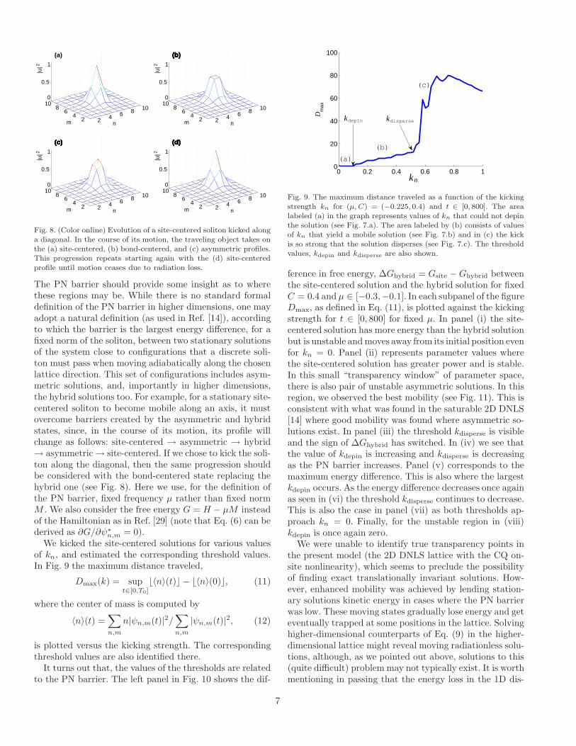
Fig. 8. (Color online) Evolution of a site-centered soliton kicked alonga diagonal. In the course of its motion, the traveling object takes onthe (a) site-centered, (b) bond-centered, and (c) asymmetric profiles.This progression repeats starting again with the (d) site-centeredprofile until motion ceases due to radiation loss.

The PN barrier should provide some insight as to wherethese regions may be. While there is no standard formaldefinition of the PN barrier in higher dimensions, one mayadopt a natural definition (as used in Ref. [14]), accordingto which the barrier is the largest energy difference, for afixed norm of the soliton, between two stationary solutionsof the system close to configurations that a discrete soli-ton must pass when moving adiabatically along the chosenlattice direction. This set of configurations includes asym-metric solutions, and, importantly in higher dimensions,the hybrid solutions too. For example, for a stationary site-centered soliton to become mobile along an axis, it mustovercome barriers created by the asymmetric and hybridstates, since, in the course of its motion, its profile willchange as follows: site-centered → asymmetric → hybrid→ asymmetric → site-centered. If we chose to kick the soli-ton along the diagonal, then the same progression shouldbe considered with the bond-centered state replacing thehybrid one (see Fig. 8). Here we use, for the definition ofthe PN barrier, fixed frequency µ rather than fixed normM . We also consider the free energy G = H − µM insteadof the Hamiltonian as in Ref. [29] (note that Eq. (6) can bederived as ∂G/∂ψ∗

n,m = 0).We kicked the site-centered solutions for various values

of kn, and estimated the corresponding threshold values.In Fig. 9 the maximum distance traveled,

Dmax(k) = supt∈[0,T0]

⌊〈n〉(t)⌋ − ⌊〈n〉(0)⌋, (11)

where the center of mass is computed by

〈n〉(t) =∑

n,m

n|ψn,m(t)|2/∑

n,m

|ψn,m(t)|2, (12)

is plotted versus the kicking strength. The correspondingthreshold values are also identified there.

It turns out that, the values of the thresholds are relatedto the PN barrier. The left panel in Fig. 10 shows the dif-

0 0.2 0.4 0.6 0.8 10

20

40

60

80

100

k n

Dm

ax

kdepin

(b)

kdisperse

(c)

(a)

Fig. 9. The maximum distance traveled as a function of the kickingstrength kn for (µ, C) = (−0.225, 0.4) and t ∈ [0, 800]. The arealabeled (a) in the graph represents values of kn that could not depinthe solution (see Fig. 7.a). The area labeled by (b) consists of valuesof kn that yield a mobile solution (see Fig. 7.b) and in (c) the kickis so strong that the solution disperses (see Fig. 7.c). The thresholdvalues, kdepin and kdisperse are also shown.

ference in free energy, ∆Ghybrid = Gsite −Ghybrid betweenthe site-centered solution and the hybrid solution for fixedC = 0.4 and µ ∈ [−0.3,−0.1]. In each subpanel of the figureDmax, as defined in Eq. (11), is plotted against the kickingstrength for t ∈ [0, 800] for fixed µ. In panel (i) the site-centered solution has more energy than the hybrid solutionbut is unstable and moves away from its initial position evenfor kn = 0. Panel (ii) represents parameter values wherethe site-centered solution has greater power and is stable.In this small “transparency window” of parameter space,there is also pair of unstable asymmetric solutions. In thisregion, we observed the best mobility (see Fig. 11). This isconsistent with what was found in the saturable 2D DNLS[14] where good mobility was found where asymmetric so-lutions exist. In panel (iii) the threshold kdisperse is visibleand the sign of ∆Ghybrid has switched. In (iv) we see thatthe value of kdepin is increasing and kdisperse is decreasingas the PN barrier increases. Panel (v) corresponds to themaximum energy difference. This is also where the largestkdepin occurs. As the energy difference decreases once againas seen in (vi) the threshold kdisperse continues to decrease.This is also the case in panel (vii) as both thresholds ap-proach kn = 0. Finally, for the unstable region in (viii)kdepin is once again zero.

We were unable to identify true transparency points inthe present model (the 2D DNLS lattice with the CQ on-site nonlinearity), which seems to preclude the possibilityof finding exact translationally invariant solutions. How-ever, enhanced mobility was achieved by lending station-ary solutions kinetic energy in cases where the PN barrierwas low. These moving states gradually lose energy and geteventually trapped at some positions in the lattice. Solvinghigher-dimensional counterparts of Eq. (9) in the higher-dimensional lattice might reveal moving radiationless solu-tions, although, as we pointed out above, solutions to this(quite difficult) problem may not typically exist. It is worthmentioning in passing that the energy loss in the 1D dis-

7

−0.25 −0.2 −0.15−0.01

−0.005

0

0.005

0.01

µ

∆ G

i

ii

iii

iv

vvi

vii

viii

0 0.2 0.4 0.6 0.8 10

20

40

60

80

100

k

D m

ax

i

0 0.2 0.4 0.6 0.8 10

20

40

60

80

100

k

ii

0 0.2 0.4 0.6 0.8 10

20

40

60

80

100

k

iii

0 0.2 0.4 0.6 0.8 10

20

40

60

80

100

k

iv

0 0.2 0.4 0.6 0.8 10

20

40

60

80

100

k

D m

ax

v

0 0.2 0.4 0.6 0.8 10

20

40

60

80

100

k

vi

0 0.2 0.4 0.6 0.8 10

20

40

60

80

100

k

vii

0 0.2 0.4 0.6 0.8 10

20

40

60

80

100

k

viii

Fig. 10. (Color online) Left: Plot of ∆Ghybrid for various values of µ and fixed C = 0.4. The remaining panels (i)–(viii) correspond to themaximum distance traveled versus kicking strength plots. See text for more details.

n5 10 15 20 25 30 35 40

100

200

300

400

500

600

700

800

−0.2835 −0.2825 −0.2815 −0.2805

−2

−1

0

1

2

x 10−4

µ

∆ G

∆ Ghybrid

∆ G asymm 1

∆ G asymm 2

Fig. 11. (Color online) Top: density plot for the site-centered solitonset in motion along the lattice axis for (µ, C) = (−0.282, 0.4) andkn = 0.5. The choice of parameters fall in a “transparency window”where good mobility is observed, possibly due to the existence of apair of asymmetric solutions. A one-dimensional slice along the axisof propagation (at m = 10) is shown here. Bottom: zoom of the leftpanel of Fig. 10 near the “transparency window”. The difference offree energy of the site-centered solution and the pair of asymmetricsolutions ∆Gasymm = Gsite − Gasymm is also shown. The energyadded from the kick exceeds both of these differences.

crete sine-Gordon lattice has been recently described usingan averaged Lagrangian approach in Ref. [40].

5. Three-dimensional solutions

We will now briefly consider a 3D version of the CQDNLS model. The respective counterpart of Eq. (5) is

iψn,m,l +C∆(3)ψn,m,l + 2|ψn,m,l|2ψn,m,l

− |ψn,m,l|4ψn,m,l = 0, (13)

where ψn,m,l is the complex field at site {n,m, l}. In anisotropic medium, the discrete Laplacian is

∆(3)ψn,m,l ≡ ψn+1,m,l + ψn−1,m,l + ψn,m+1,l + ψn,m−1,l

+ψn,m,l+1 + ψn,m,l−1 − 6ψn,m,l. (14)

We search for stationary solutions,ψn,m,l = un,m,l exp(−iµt),using the same method as in Sec. 2. The 2D soliton specieshave their natural 3D counterparts. As shown in Fig. 12,the extra dimension admits an additional type of a hybridsoliton.

Fig. 12. (Color online) Plot of the basic configurations in the 3Dlattices using iso-contours. Top: plot of 3D site-centered (left) andbond-centered (right) solitons. Larger diamonds correspond to largerlocal amplitudes. Bottom: Two different types of 3D hybrid solutions.The different colors (arranged in a 3D check-board pattern) are solelyused for clarity of presentation.

Figure 13 shows M(µ) curves for 3D bond-centered andsite-centered solitons for C = 0.1 and C = 0.7. The figureillustrates that in the 3D case, similarly to the 2D case, thesnake-like patterns are present for small values of coupling

8

−1 −0.8 −0.6 −0.4 −0.2 00

2

4

6

8

10

12

µ

M

−1 −0.8 −0.6 −0.4 −0.2 00

20

40

60

80

100

µ

M

Fig. 13. (Color online) The power of the site- and bond-centeredsolitons versus the frequency for C = 0.1 (top) and C = 0.7 (bottom)in the 3D lattice.

constant C and are stretched as C is increased. Similarresults were obtained for the 3D hybrid solutions (resultsnot shown here).

6. Variational approximation

Following the pattern of the VA developed in Ref. [24]for 1D discrete solitons in the CQ-DNLS model, it is possi-ble to construct analytical approximations for the discretesolitons, and compare them to the numerical solutions de-scribed above. We present this approach for the 2D model,but the procedure is essentially the same in three dimen-sions. It is relevant to mention that the VA for 1D discretesolitons in models of the DNLS type was first developed inRef. [41].

Solutions to the stationary version Eq. (1) are local ex-trema of the corresponding Lagrangian,

L=

∞∑

n,m=−∞

µu2n,m + u4

n,m −1

3u6

n,m (15)

−C[

(un+1,m − un,m)2 + (un,m+1 − un,m)2]

[recall ψn,m = un,m exp(−iµt)]. We approximate each soli-ton by a localized ansatz which makes it possible to evaluatethe infinite sums in Eq. (15) in an explicit form. First, thefollowing ansatz is used for the site-centered (sc) solution:

−1 −0.8 −0.6 −0.4 −0.2 00

2

4

6

8

10

µ

M

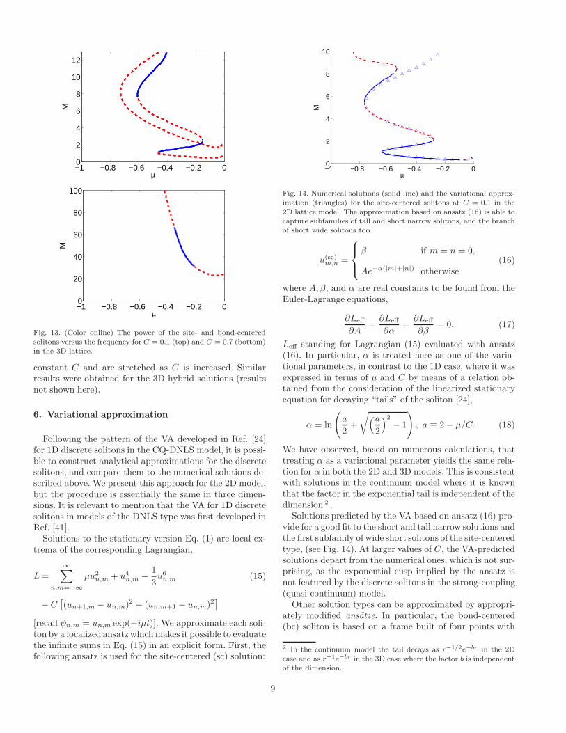
Fig. 14. Numerical solutions (solid line) and the variational approx-imation (triangles) for the site-centered solitons at C = 0.1 in the2D lattice model. The approximation based on ansatz (16) is able tocapture subfamilies of tall and short narrow solitons, and the branchof short wide solitons too.

u(sc)m,n =

β if m = n = 0,

Ae−α(|m|+|n|) otherwise(16)

where A, β, and α are real constants to be found from theEuler-Lagrange equations,

∂Leff

∂A=∂Leff

∂α=∂Leff

∂β= 0, (17)

Leff standing for Lagrangian (15) evaluated with ansatz(16). In particular, α is treated here as one of the varia-tional parameters, in contrast to the 1D case, where it wasexpressed in terms of µ and C by means of a relation ob-tained from the consideration of the linearized stationaryequation for decaying “tails” of the soliton [24],

α = ln

(

a

2+

√

(a

2

)2

− 1

)

, a ≡ 2 − µ/C. (18)

We have observed, based on numerous calculations, thattreating α as a variational parameter yields the same rela-tion for α in both the 2D and 3D models. This is consistentwith solutions in the continuum model where it is knownthat the factor in the exponential tail is independent of thedimension 2 .

Solutions predicted by the VA based on ansatz (16) pro-vide for a good fit to the short and tall narrow solutions andthe first subfamily of wide short solitons of the site-centeredtype, (see Fig. 14). At larger values of C, the VA-predictedsolutions depart from the numerical ones, which is not sur-prising, as the exponential cusp implied by the ansatz isnot featured by the discrete solitons in the strong-coupling(quasi-continuum) model.

Other solution types can be approximated by appropri-ately modified ansatze. In particular, the bond-centered(bc) soliton is based on a frame built of four points with

2 In the continuum model the tail decays as r−1/2e−br in the 2Dcase and as r−1e−br in the 3D case where the factor b is independentof the dimension.

9

−1 −0.8 −0.6 −0.4 −0.2 00

2

4

6

8

µ

M

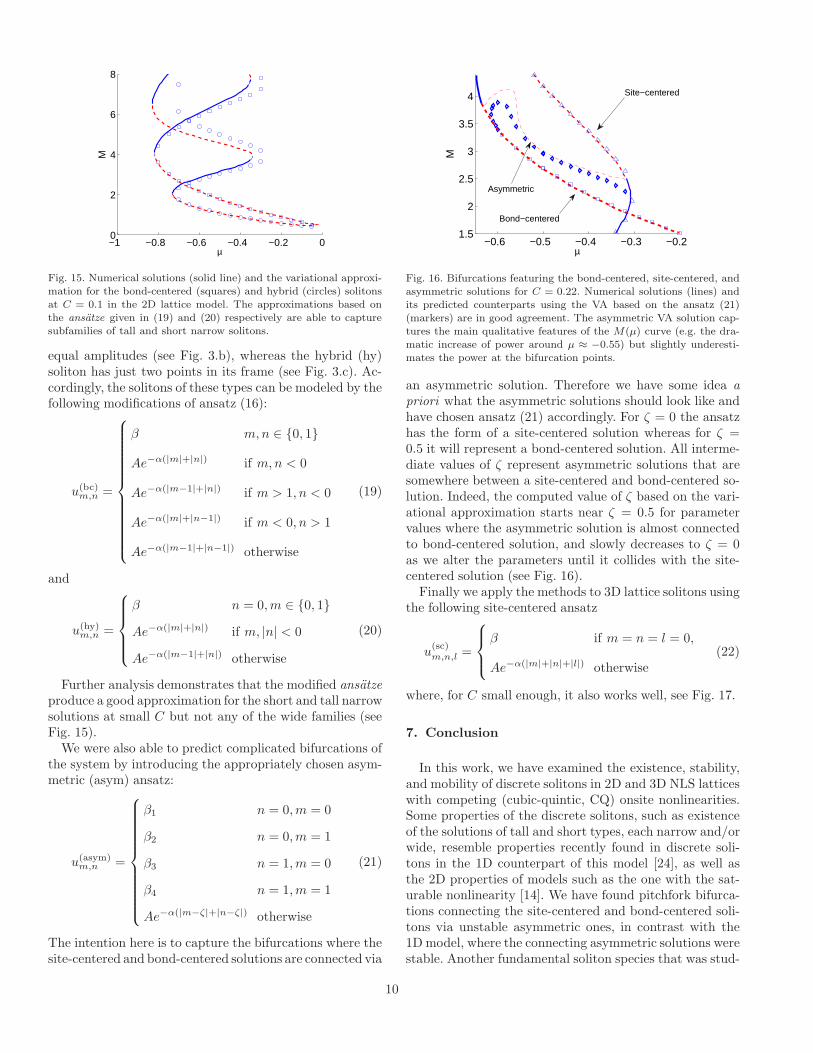
Fig. 15. Numerical solutions (solid line) and the variational approxi-mation for the bond-centered (squares) and hybrid (circles) solitonsat C = 0.1 in the 2D lattice model. The approximations based onthe ansatze given in (19) and (20) respectively are able to capturesubfamilies of tall and short narrow solitons.

equal amplitudes (see Fig. 3.b), whereas the hybrid (hy)soliton has just two points in its frame (see Fig. 3.c). Ac-cordingly, the solitons of these types can be modeled by thefollowing modifications of ansatz (16):

u(bc)m,n =

β m, n ∈ {0, 1}

Ae−α(|m|+|n|) if m,n < 0

Ae−α(|m−1|+|n|) if m > 1, n < 0

Ae−α(|m|+|n−1|) if m < 0, n > 1

Ae−α(|m−1|+|n−1|) otherwise

(19)

and

u(hy)m,n =

β n = 0,m ∈ {0, 1}

Ae−α(|m|+|n|) if m, |n| < 0

Ae−α(|m−1|+|n|) otherwise

(20)

Further analysis demonstrates that the modified ansatze

produce a good approximation for the short and tall narrowsolutions at small C but not any of the wide families (seeFig. 15).

We were also able to predict complicated bifurcations ofthe system by introducing the appropriately chosen asym-metric (asym) ansatz:

u(asym)m,n =

β1 n = 0,m = 0

β2 n = 0,m = 1

β3 n = 1,m = 0

β4 n = 1,m = 1

Ae−α(|m−ζ|+|n−ζ|) otherwise

(21)

The intention here is to capture the bifurcations where thesite-centered and bond-centered solutions are connected via

−0.6 −0.5 −0.4 −0.3 −0.21.5

2

2.5

3

3.5

4

µ

M

Bond−centered

Site−centered

Asymmetric

Fig. 16. Bifurcations featuring the bond-centered, site-centered, andasymmetric solutions for C = 0.22. Numerical solutions (lines) andits predicted counterparts using the VA based on the ansatz (21)(markers) are in good agreement. The asymmetric VA solution cap-tures the main qualitative features of the M(µ) curve (e.g. the dra-matic increase of power around µ ≈ −0.55) but slightly underesti-mates the power at the bifurcation points.

an asymmetric solution. Therefore we have some idea a

priori what the asymmetric solutions should look like andhave chosen ansatz (21) accordingly. For ζ = 0 the ansatzhas the form of a site-centered solution whereas for ζ =0.5 it will represent a bond-centered solution. All interme-diate values of ζ represent asymmetric solutions that aresomewhere between a site-centered and bond-centered so-lution. Indeed, the computed value of ζ based on the vari-ational approximation starts near ζ = 0.5 for parametervalues where the asymmetric solution is almost connectedto bond-centered solution, and slowly decreases to ζ = 0as we alter the parameters until it collides with the site-centered solution (see Fig. 16).

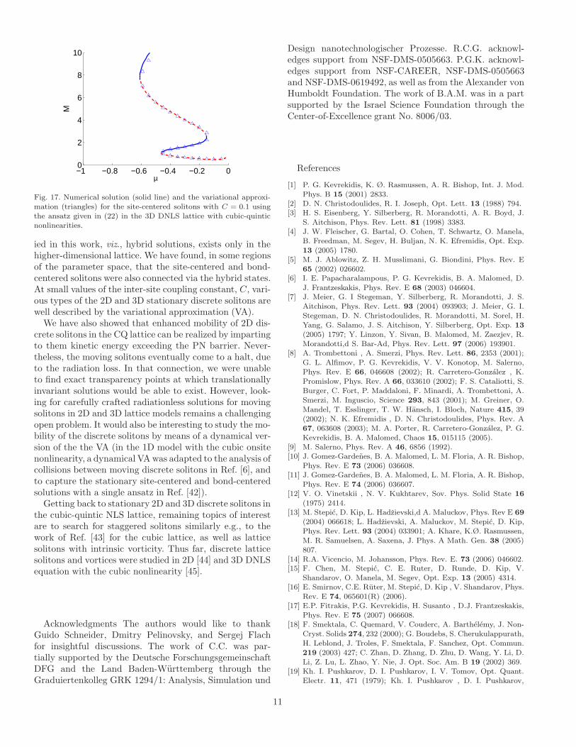
Finally we apply the methods to 3D lattice solitons usingthe following site-centered ansatz

u(sc)m,n,l =

β if m = n = l = 0,

Ae−α(|m|+|n|+|l|) otherwise(22)

where, for C small enough, it also works well, see Fig. 17.

7. Conclusion

In this work, we have examined the existence, stability,and mobility of discrete solitons in 2D and 3D NLS latticeswith competing (cubic-quintic, CQ) onsite nonlinearities.Some properties of the discrete solitons, such as existenceof the solutions of tall and short types, each narrow and/orwide, resemble properties recently found in discrete soli-tons in the 1D counterpart of this model [24], as well asthe 2D properties of models such as the one with the sat-urable nonlinearity [14]. We have found pitchfork bifurca-tions connecting the site-centered and bond-centered soli-tons via unstable asymmetric ones, in contrast with the1D model, where the connecting asymmetric solutions werestable. Another fundamental soliton species that was stud-

10

−1 −0.8 −0.6 −0.4 −0.2 00

2

4

6

8

10

µ

M

Fig. 17. Numerical solution (solid line) and the variational approxi-mation (triangles) for the site-centered solitons with C = 0.1 usingthe ansatz given in (22) in the 3D DNLS lattice with cubic-quinticnonlinearities.

ied in this work, viz., hybrid solutions, exists only in thehigher-dimensional lattice. We have found, in some regionsof the parameter space, that the site-centered and bond-centered solitons were also connected via the hybrid states.At small values of the inter-site coupling constant, C, vari-ous types of the 2D and 3D stationary discrete solitons arewell described by the variational approximation (VA).

We have also showed that enhanced mobility of 2D dis-crete solitons in the CQ lattice can be realized by impartingto them kinetic energy exceeding the PN barrier. Never-theless, the moving solitons eventually come to a halt, dueto the radiation loss. In that connection, we were unableto find exact transparency points at which translationallyinvariant solutions would be able to exist. However, look-ing for carefully crafted radiationless solutions for movingsolitons in 2D and 3D lattice models remains a challengingopen problem. It would also be interesting to study the mo-bility of the discrete solitons by means of a dynamical ver-sion of the the VA (in the 1D model with the cubic onsitenonlinearity, a dynamical VA was adapted to the analysis ofcollisions between moving discrete solitons in Ref. [6], andto capture the stationary site-centered and bond-centeredsolutions with a single ansatz in Ref. [42]).

Getting back to stationary 2D and 3D discrete solitons inthe cubic-quintic NLS lattice, remaining topics of interestare to search for staggered solitons similarly e.g., to thework of Ref. [43] for the cubic lattice, as well as latticesolitons with intrinsic vorticity. Thus far, discrete latticesolitons and vortices were studied in 2D [44] and 3D DNLSequation with the cubic nonlinearity [45].

Acknowledgments The authors would like to thankGuido Schneider, Dmitry Pelinovsky, and Sergej Flachfor insightful discussions. The work of C.C. was par-tially supported by the Deutsche ForschungsgemeinschaftDFG and the Land Baden-Wurttemberg through theGraduiertenkolleg GRK 1294/1: Analysis, Simulation und

Design nanotechnologischer Prozesse. R.C.G. acknowl-edges support from NSF-DMS-0505663. P.G.K. acknowl-edges support from NSF-CAREER, NSF-DMS-0505663and NSF-DMS-0619492, as well as from the Alexander vonHumboldt Foundation. The work of B.A.M. was in a partsupported by the Israel Science Foundation through theCenter-of-Excellence grant No. 8006/03.

References

[1] P. G. Kevrekidis, K. Ø. Rasmussen, A. R. Bishop, Int. J. Mod.Phys. B 15 (2001) 2833.

[2] D. N. Christodoulides, R. I. Joseph, Opt. Lett. 13 (1988) 794.[3] H. S. Eisenberg, Y. Silberberg, R. Morandotti, A. R. Boyd, J.

S. Aitchison, Phys. Rev. Lett. 81 (1998) 3383.[4] J. W. Fleischer, G. Bartal, O. Cohen, T. Schwartz, O. Manela,

B. Freedman, M. Segev, H. Buljan, N. K. Efremidis, Opt. Exp.13 (2005) 1780.

[5] M. J. Ablowitz, Z. H. Musslimani, G. Biondini, Phys. Rev. E65 (2002) 026602.

[6] I. E. Papacharalampous, P. G. Kevrekidis, B. A. Malomed, D.

J. Frantzeskakis, Phys. Rev. E 68 (2003) 046604.[7] J. Meier, G. I Stegeman, Y. Silberberg, R. Morandotti, J. S.

Aitchison, Phys. Rev. Lett. 93 (2004) 093903; J. Meier, G. I.Stegeman, D. N. Christodoulides, R. Morandotti, M. Sorel, H.Yang, G. Salamo, J. S. Aitchison, Y. Silberberg, Opt. Exp. 13

(2005) 1797; Y. Linzon, Y. Sivan, B. Malomed, M. Zaezjev, R.Morandotti,d S. Bar-Ad, Phys. Rev. Lett. 97 (2006) 193901.

[8] A. Trombettoni , A. Smerzi, Phys. Rev. Lett. 86, 2353 (2001);G. L. Alfimov, P. G. Kevrekidis, V. V. Konotop, M. Salerno,Phys. Rev. E 66, 046608 (2002); R. Carretero-Gonzalez , K.Promislow, Phys. Rev. A 66, 033610 (2002); F. S. Cataliotti, S.Burger, C. Fort, P. Maddaloni, F. Minardi, A. Trombettoni, A.Smerzi, M. Inguscio, Science 293, 843 (2001); M. Greiner, O.Mandel, T. Esslinger, T. W. Hansch, I. Bloch, Nature 415, 39(2002); N. K. Efremidis , D. N. Christodoulides, Phys. Rev. A67, 063608 (2003); M. A. Porter, R. Carretero-Gonzalez, P. G.Kevrekidis, B. A. Malomed, Chaos 15, 015115 (2005).

[9] M. Salerno, Phys. Rev. A 46, 6856 (1992).[10] J. Gomez-Gardenes, B. A. Malomed, L. M. Floria, A. R. Bishop,

Phys. Rev. E 73 (2006) 036608.[11] J. Gomez-Gardenes, B. A. Malomed, L. M. Floria, A. R. Bishop,

Phys. Rev. E 74 (2006) 036607.[12] V. O. Vinetskii , N. V. Kukhtarev, Sov. Phys. Solid State 16

(1975) 2414.[13] M. Stepic, D. Kip, L. Hadzievski,d A. Maluckov, Phys. Rev E 69

(2004) 066618; L. Hadzievski, A. Maluckov, M. Stepic, D. Kip,Phys. Rev. Lett. 93 (2004) 033901; A. Khare, K.Ø. Rasmussen,M. R. Samuelsen, A. Saxena, J. Phys. A Math. Gen. 38 (2005)807.

[14] R.A. Vicencio, M. Johansson, Phys. Rev. E. 73 (2006) 046602.[15] F. Chen, M. Stepic, C. E. Ruter, D. Runde, D. Kip, V.

Shandarov, O. Manela, M. Segev, Opt. Exp. 13 (2005) 4314.[16] E. Smirnov, C.E. Ruter, M. Stepic, D. Kip , V. Shandarov, Phys.

Rev. E 74, 065601(R) (2006).[17] E.P. Fitrakis, P.G. Kevrekidis, H. Susanto , D.J. Frantzeskakis,

Phys. Rev. E 75 (2007) 066608.[18] F. Smektala, C. Quemard, V. Couderc, A. Barthelemy, J. Non-

Cryst. Solids 274, 232 (2000); G. Boudebs, S. Cherukulappurath,H. Leblond, J. Troles, F. Smektala, F. Sanchez, Opt. Commun.219 (2003) 427; C. Zhan, D. Zhang, D. Zhu, D. Wang, Y. Li, D.Li, Z. Lu, L. Zhao, Y. Nie, J. Opt. Soc. Am. B 19 (2002) 369.

[19] Kh. I. Pushkarov, D. I. Pushkarov, I. V. Tomov, Opt. Quant.Electr. 11, 471 (1979); Kh. I. Pushkarov , D. I. Pushkarov,

11

Rep. Math. Phys. 17, 37 (1980); S. Cowan, R. H. Enns, S. S.Rangnekar, S. S. Sanghera, Can. J. Phys. 64, 311 (1986); J.Herrmann, Opt. Commun. 87, 161 (1992).

[20] I. M. Merhasin, B. V. Gisin, R. Driben, B. A. Malomed,Phys. Rev. E 71, 016613 (2005); see also works in which thecubic-quintic nonlinearity is combined with a sinusoidal one-dimensional potential: J. Wang, F. Ye, L. Dong, T. Cai, Y.-P. Li,Phys. Lett. A 339, 74 (2005); F. Abdullaev, A. Abdumalikov,R. Galimzyanov, Phys. Lett. A 367, 149 (2007).

[21] R. Driben, B. A. Malomed, A. Gubeskys, J. Zyss, Phys. Rev. E76 (2007) 066604.

[22] I. Bloch, Nature Phys. 1 (2005) 23.[23] A. E. Muryshev, G. V. Shlyapnikov, W. Ertmer, K. Sengstock,

M. Lewenstein, Phys. Rev. Lett. 89, 110401 (2002); L. D. Carr, J.Brand, ibid. 92, 040401 (2004); Phys. Rev. A 70, 033607 (2004);L. Khaykovich , B. A. Malomed, ibid. A 74, 023607 (2006).

[24] R. Carretero-Gonzales, J. D. Talley, C. Chong, B. A. Malomed,Physica D 216, 77 (2006).

[25] A. Maluckov, L. Hadzievski, B. A. Malomed, Phys. Rev. E 76,046605 (2007).

[26] A. Maluckov, L. Hadzievski, B.A. Malomed, submitted forpublication.

[27] M. Oster, M. Johansson, A. Eriksson, Phys. Rev. E. 67 (2003)056606.

[28] C. Chong, M.S. Thesis, San Diego State University (2006).[29] T.R.O. Melvin, P.G. Kevrekidis, J. Cuevas Phys. Rev. Lett.

97 (2006) 124101; T.R.O. Melvin, A.R. Champneys, P.G.Kevrekidis , J. Cuevas, Travelling solitary waves in the discrete

Schrodinger equation with saturable nonlinearity: Existence,

stability and dynamics, Physica D (2008) in press.[30] T. Bountis, H. W. Capel, M. Kollmann, J. C. Ross, J. M.

Bergamin, J.P. van der Weele, Phys. Lett. A 268 (2000) 50.[31] G. L. Alfimov, V. A. Brazhnyi, V. V. Konotop. Physica D 194

(2004) 127.[32] P.G. Kevrekidis, K.Ø. Rasmussen, A.R. Bishop, Phys. Rev. E

61 (2000) 2006.[33] S. Flach, K. Kladko, R. S. MacKay 78 (1997) 1207.[34] M.I. Weinstein, Nonlinearity 12 (1999) 673.[35] P.G. Kevrekidis, Physica D 183 (2003) 68.[36] D.E. Pelinovsky, Nonlinearity 19 (2006) 2695.[37] D.E. Pelinovsky, T.R.O. Melvin, A.R. Champneys, Physica D

236 (2007) 22.[38] H. Susanto, P. G. Kevrekidis, R. Carretero-Gonzalez, B. A.

Malomed, D. J. Frantzeskakis, Phys. Rev. Lett. 99 (2007)214103.

[39] O. Bang, P.D. Miller, Phys. Scr. T67 (2003) 26.[40] L.A. Cisneros , A.A. Minzoni, Physcia D 237 (2008) 50.[41] B. Malomed , M.I. Weinstein, Phys. Lett. A 220 (1996) 91.[42] D.J. Kaup, Math. Comput. Simulat. 69 (2005) 322.[43] P.G. Kevrekidis, H. Susanto , Z. Chen, Phys. Rev. E 74, 066606

(2006).[44] For a compendium of relevant solutions, see e.g., D.E. Pelinovsky,

P.G. Kevrekidis , D.J. Frantzeskakis, Physica D 212, 20 (2005).[45] P.G. Kevrekidis, B.A. Malomed, D.J. Frantzeskakis, R.

Carretero-Gonzalez, Phys. Rev. Lett. 93 (2004) 080403; R.Carretero-Gonzalez, P.G. Kevrekidis, B.A. Malomed, D.J.Frantzeskakis, ibid. 94 (2005) 203901; M. Lukas, D. Pelinovsky,P.G. Kevrekidis, Physica D 237, 339 (2008).

12