Multiscale Simulations Using Generalized Interpolation Material Point ... · ized interpolation material point (GIMP) method, Bar-denhagen and Kober (2004), ... ρw·bsdΩ, (1) where

Copyright c© 2005 Tech Science Press CMES, vol.8, no.2, pp.135-152, 2005

Multiscale Simulations Using Generalized Interpolation Material Point (GIMP)Method And SAMRAI Parallel Processing

J. Ma1, H. Lu1, B. Wang1, S. Roy1, R. Hornung2, A. Wissink2 and R. Komanduri1,3

Abstract: In the simulation of a wide range of mechan-ics problems including impact/contact/penetration andfracture, the material point method (MPM), Sulsky, Zhouand Shreyer (1995), demonstrated its computational ca-pabilities. To resolve alternating stress sign and insta-bility problems associated with conventional MPM, Bar-denhagen and Kober (2004) introduced recently the gen-eralized interpolation material point (GIMP) method andimplemented for one-dimensional simulations. In thispaper we have extended GIMP to 2D and applied to sim-ulate simple tension and indentation problems. For sim-ulations spanning multiple length scales, based on thecontinuum mechanics approach, we present a parallelGIMP computational method using the Structured Adap-tive Mesh Refinement Application Infrastructure (SAM-RAI). SAMRAI is used for multi-processor distributedmemory computations, as a platform for domain decom-position, and for multi-level refinement of the computa-tional domain. Nested computational grid levels (withsuccessive spatial and temporal refinements) are used inGIMP simulations to improve the computational accu-racy and to reduce the overall computational time. Thedomain of each grid level is divided into multiple rect-angular patches for parallel processing. This domain de-composition embedded in SAMRAI is very flexible whenapplied to GIMP. As an example to validate the parallelGIMP computing scheme under SAMRAI parallel com-puting environment, numerical simulations with multi-ple length scales from nanometer to millimeter were con-ducted on a 2D nanoindentation problem. A contact al-

1 School of Mechanical and Aerospace Engineering, OklahomaState University, Stillwater, OK 74078, U.S.A2 Center for Applied Scientific Computing, Lawrence LivermoreNational Laboratory, Livermore, CA 94551, U.S.A3 Correspondence author, e-mail: [email protected]; Tel:405-744-5900; Fax: 405-744-7873.This work was performed under the auspices of the U.S. Depart-ment of Energy by University of California, Lawrence LivermoreNational Laboratory under Contract W-7405-Eng-48. UCRL-JRNL-208241.

gorithm in GIMP has also been developed for the treat-ment of contact pair between a rigid indenter and a de-formable workpiece. GIMP results are compared withfinite element results on indentation for validation. AGIMP nanoindentation problem with five levels of refine-ment was modeled using multi-processors to demonstratethe potential capability of the parallel GIMP computa-tion.

keyword: Material point method (MPM), Generalizedinterpolation material point method (GIMP), Tension,Nanoindentation, Parallel computing, SAMRAI, Multi-level refinement, Contact problem.

1 Introduction

The material point method (MPM) has demonstrated itscapabilities in addressing such problems as impact, up-setting, penetration, and contact (e.g. Sulsky, Zhou andSchreyer (1995); Sulsky and Schreyer (1996)). In MPM,two descriptions are used – one based on a collection ofmaterial points (Lagrangian) and the other based on acomputational background grid (Eulerian), as proposedby Sulsky, Zhou and Schreyer (1995). A fixed struc-tured mesh is generally used in the background through-out the MPM simulations. The material points are fol-lowed throughout the deformation of a solid to providea Lagrangian description and the governing field equa-tions are solved at the background grid nodes so thatMPM is not subject to mesh entanglement. Comparedto the finite element method (FEM), MPM takes ad-vantage of both Eulerian and Lagrangian descriptionsand possesses the capability of handling large defor-mations in a more natural manner so that mesh lock-up problems present in FEM are avoided. Addition-ally, for problems involving contact, MPM provides anaturally non-slip contact algorithm to avoid the pene-tration between two bodies based on a common back-ground mesh (Sulsky, Zhou and Schreyer (1995), Sul-

136 Copyright c© 2005 Tech Science Press CMES, vol.8, no.2, pp.135-152, 2005

sky and Schreyer (1996)). One drawback of the con-ventional MPM is that when the material points moveacross the cell boundaries during deformation, some nu-merical noise/errors can be generated, Bardenhagen andKober (2004). To solve the instability problems asso-ciated with the conventional MPM simulations, Barden-hagen and Kober recently proposed the generalized inter-polation material point method (GIMP) and implementedfor one-dimensional simulations.

The present investigation extends the GIMP presentedby Bardenhagen-Kober to two-dimensional simulationsand applies it to simple tension and indentation problems.Furthermore, a refinement technique and a parallel pro-cessing scheme are developed so that the serial GIMP al-gorithm and code can be extended for parallel computa-tion of large scale computations based on the continuummechanics approach.

Parallel processing has been used successfully in nu-merical analysis using different methods, such as FEMand boundary element method (BEM), Mackerle (2003)and molecular dynamics (MD), Kalia and Nakano(1993). The computational time on parallel processorscan be reduced to a small fraction of the time con-sumed by a single processor at the same speed. Par-allel processing generally involves issues, such as do-main decomposition/partitioning, load balancing, par-allel solver/algorithms, parallel mesh generation, andmulti-grid, Mackerle (2003). Domain decomposition hasbeen widely applied in parallel processing in FEM, Hsien(1997). With partitioning of the overall computationaldomain, sequential FEM algorithm usually cannot beused directly in parallel processing without some modifi-cation, primarily due to the coupling of a large number ofsimultaneous linear equations. Remeshing is sometimesneeded in each sub-domain. The interfaces of neighbor-ing sub-domains must be meshed identically for subse-quent communications, Mackerle (2003). These prob-lems are intrinsic to certain numerical methods, such asFEM; however, they can be totally or partially avoided ifother appropriate computational methods are used. Forexample, the domain decomposition is more straightfor-ward for structured meshes, and large systems of coupledequations can be avoided, if explicit time integration isused.

Recently a platform for parallel computation, namely, thestructured adaptive mesh refinement application infras-tructure (SAMRAI), Hornung and Kohn (2002), has been

developed by the Center for Applied Scientific Com-puting at the Lawrence Livermore National Laboratory.SAMRAI has provided interfaces for user-defined datatypes so that material points carrying physical variables(mass, displacement, velocity, acceleration, stress, strain,etc.) can be readily defined. As a result, SAMRAI is verysuitable for handling material points and their physicalvariables in MPM or its variant, GIMP. In this investi-gation SAMRAI is used for parallelizing GIMP. SAM-RAI has also provided a foundation for parallel adap-tive mesh refinement (AMR) with the use of either dy-namic or static load balancing, Wissink, Hysom and Hor-nung (2003). This function allows SAMRAI to processboth spatial and temporal refinements in areas of inter-est, typically with high gradients in some physical vari-ables (e.g., strains), and to use coarse mesh in the remain-ing areas. With the appropriate use of fine and coarsemeshes in different regions, multiscale simulations us-ing MPM can provide desired computational accuracywith reduced costs associated with computer memoryand computational time.

Material multiscale simulations span from elec-tronic structure, atomistic scale, crystal scale, tomacro/continuum scale, Horstemeyer, Baskes, Prantil,Philliber and Vonderheide (2003); Komanduri, Lu,Roy, Wang and Raff (2004). Appropriate simulationalgorithms can be used at various scales, e.g., abinitio computation for electronic structure, moleculardynamics at the atomistic scale, crystal plasticity ormesoplasticity at the crystal scale, and continuum me-chanics at the macro scale, Horstemeyer, Baskes, Prantil,Philliber and Vonderheide (2003). At the continuumscale, FEM is generally used. Recently, the meshlesslocal Petrov-Galerkin (MLPG) method (Shen and Atluri(2004a, 2005)) and the continuum/lattice Green functionmethod (Tewary and Read (2004)) have been used tocouple with molecular dynamics seamlessly. The MLPGmethod is a simple, less-costly alternative approachto FEM, Atluri and Shen (2002). For the purposes ofproviding the insights into the discrete atomistic systemand coupling with continuum, an equivalent continuumwas defined in the MD region to compute the atomicstress based on the Smoothed Particle Hydrodynamics(SPH) method, Shen and Atluri (2004b). The atomicstress tensor computed using the SPH method is morenatural than other atomic stress formulations becauseit is in the nonvolume-averaged form and rigorously

Multiscale Simulations Using Generalized Interpolation Material Point (GIMP) Method And SAMRAI Parallel Processing137

satisfies the conservation of linear momentum. Hence, itis applicable to both homogeneous and inhomogeneousdeformations. A tangent stiffness formulation wasdeveloped for both MLPG and MD regions and thedisplacements of the nodes and atoms are solved in onecoupled set of linear equations. The MLPG/MD cou-pling has been demonstrated to be capable of enforcingthe local balance equations in the handshaking regionbetween continuum mechanics and molecular dynamics,Shen and Atluri (2005).

The simulation using parallel GIMP computing schemein this investigation will focus on multiscales, e.g., fromnanometer to millimeter, based on the continuum me-chanics approach, namely, 2D GIMP. An example usedfor validating the simulation at several length scales atthe continuum level is nanoindentation. It involves thecontact issue between a rigid indenter and a deformableworkpiece. A contact algorithm, which allows the con-tact interface to be located in a few computational do-mains, is introduced in this study. The contact pressure isdetermined from solving a set of equations from multipleprocessors. Parallel GIMP results on nanoindentation arecompared with FEM results using the ABAQUS/Explicitcode. A nanoindentation model with five levels will beused; this model allows simulation from nanometer tomillimeter scales.

2 Generalized Interpolation Material Point (GIMP)Method

The governing equations in both conventional materialpoint method (MPM), Sulsky, Zhou and Sheryer (1995),Hu and Chen (2003), Bardenhagen (2002) and general-ized interpolation material point (GIMP) method, Bar-denhagen and Kober (2004), are briefly summarized inthis section. The weak form of the momentum conserva-tion equation in the conventional MPM is given by∫

Ωρw ·adΩ = −

∫Ω

ρss : ∇wdΩ

+∫

∂Ωρcs ·wdS +

∫Ω

ρw ·bsdΩ, (1)

where w is the test function, a is the acceleration, andss, cs and bs are the specific stress, specific traction, andspecific body force, respectively. Ω is the current con-figuration and ∂Ω is the surface with applied traction.The material density, ρ, can be approximated as the sumof material point masses using a Dirac delta function

ρ(x, t) =Np

∑p=1

Mpδ(x−xtp), where Np is the total num-

ber of material points and Mp is the mass of the ma-terial point. Upon discretization of Eq. (1) using theshape functions Ni(xt

p), the governing equations at thebackground grid nodes become (see Sulsky, Zhou andSchreyer (1995))

mtia

ti = (ft

i)int +(ft

i)ext . (2)

where the lumped mass matrix is given by

mti =

Np

∑p=1

MpNi(xtp), (3)

and the internal and external forces are given by

(fti)

int = −Np

∑p=1

Mpss,tp · ∇Ni|xt

p, (4)

(fti)

ext = −Np

∑p=1

Mpcs,tp h−1Ni(xt

p)+Np

∑p=1

MpbtpNi(xt

p), (5)

where h is the thickness of a boundary layer. At each timestep, all variables for each material point, such as mass,velocity, and force are extrapolated to the grid nodes ofthe cell in which the material point resides. New nodalmomenta are computed and used to update the physi-cal variables carried by the material points. Thus, ma-terial points move relative to each other to represent de-formation in a solid. A spatially fixed background gridis used throughout the MPM computation. MPM hasalready demonstrated its capabilities in solving a num-ber of problems involving impact/contact/penetration. Incase of large deformation, however, numerical noise,or errors have been observed, especially when materialpoints have just crossed cell boundaries resulting in insta-bility problems in the MPM simulations (see, e.g., Sul-sky, Zhou and Schreyer (1995), Hu and Chen (2003),Bardenhagen and Kober (2004)). The primary cause forthe problem has been attributed to the discontinuity ofthe gradient of the shape functions across the cell bound-aries (see, e.g., Hu and Chen (2003), Bardenhagen andKober (2004)). To resolve this problem, Bardenhagenand Kober (2004) proposed a generalized interpolationmaterial point (GIMP) method. In GIMP, the interpola-tion between node i and material point p is given by thevolume averaged weighting function

Sip =1

Vp

∫

Ω∩Ωp

χp(x)Si(x)dx, (6)


where Vp is the current volume of the material point,χp(x) is the characteristic function of the material point,and Si(x) is the node shape function. The role of theweighting function is the same as the shape function inconventional MPM. The modified equation of momen-tum conservation, Bardenhagen and Kober (2004), canbe written as

∑p

∫

Ω∩Ωp

ppχp

Vp·δvdx+∑

p

∫

Ω∩Ωp

σpχp : δvdx

= ∑p

∫

Ω∩Ωp

mpχp

Vpb ·δvdx+

∫

∂Ω

c ·δvdx, (7)

where δv is an admissible velocity field, pp is the rate ofchange of the material point momentum. Eq. (7) can befurther discretized and solved at the grid nodes, Barden-hagen and Kober (2004). Herein, the weighting functionSip is C1 continuous under the spatially fixed backgroundgrid. Consequently the noises associated with materialpoint crossing cell boundaries in the conventional MPMcan be minimized.

In this paper, we have implemented GIMP presentedby Bardenhagen-Kober for two-dimensional simulations.We have also developed a refinement technique and a par-allel processing scheme to extend the serial GIMP algo-rithm to code large scale parallel computing. The ca-pability of parallel GIMP computing has been demon-strated by modeling nanoindentation problem. A con-tact algorithm has been developed to address the contactproblem between the rigid indenter and the deformableworkpiece. We proceed next to describe the contact al-gorithm developed in this investigation.

2.1 Contact Algorithm in GIMP

Nanoindentation involves a contact pair of a rigid inden-ter and a deformable workpiece. The contact interac-tion between these two surfaces is governed by the New-ton’s third law and Coulomb’s friction law as well as theboundary compatibility condition at the contact interface,Oden and Pires (1983), Zhong (1993). While MPM canprevent the penetration at the interface automatically, ituses a single mesh for the two bodies. At the contact sur-face, all components of the variables are interpolated tothe nodes from both bodies using Eqs. (3)-(5). As a re-sult, MPM using a single mesh tends to induce early con-tact in approaching and late separation when two partsmove away from each other. So, MPM cannot model

the contact behavior between two parts correctly. Hu andChen (2003) proposed a multi-mesh MPM algorithm torelease the no-slip constraint inherent in the MPM usinga single mesh. In the multi-mesh MPM, in addition to acommon mesh for all objects, there is an individual meshfor each of the objects under consideration. All meshesare identical, i.e. nodal locations are the same. The multi-mesh can be generated by creating multiple nodal fieldsfor each node. Each nodal field corresponds to an ob-ject. In multi-mesh MPM scheme, the nodal masses andforces are mapped from the material points of each ob-ject to its own mesh. The nodal values are transferredto the corresponding nodes in the common mesh. Whenthe values at a node of the common background mesh in-volve contributions from two parts, the contact betweentwo parts occurs so that this node is defined as an over-lapped node. Otherwise, two parts move independently.This multi-mesh algorithm can handle sliding and sepa-ration for the contact pair. However, in using the multi-mesh for contact problem in GIMP, the interaction at theoverlapped nodes is still activated too early before theactual contact of the material points occurs.

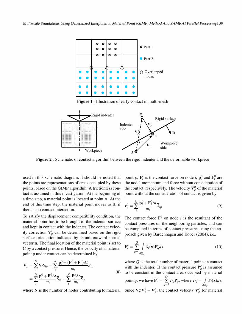
Fig. 1 is an example illustrating early contact when Part1 is moving toward Part 2. The four bottom particles ofPart 1, labeled in hollow circles, have come into the cellsof Part 2, the nodes of which cells are labeled in threedashed circles. Physical variables (e.g., normal force,and velocity component normal to the contact surface)in Part 1 will be interpolated onto these three overlappednodes. The physical variables in the three overlappednodes will be further interpolated into material pointswithin the top layer of cells in Part 2, and contributeto the stress and deformation in the entire Part 2. Withthis treatment in the previous multi-mesh algorithm, eventhough Parts 1 and 2 are not in physical contact, the par-ticles in Part 2 will contribute to the physical variables ofparticles in Part 1, leading to numerical early contact, andvice versa, through the overlapped nodes. Similar situa-tion occurs when Part 1 is retracting from Part 2, resultingin late separation of two parts. Unless other measures aretaken to prevent these physically incorrect early contactand late separation problems, they could cause large er-rors in GIMP and must be corrected in contact problems.

In this paper, a new contact algorithm is developed forGIMP simulations. Fig. 2 illustrates the contact algo-rithm for the contact pair between a rigid indenter anda deformable workpiece. Although circular points are


Part 1

Part 2

Overlapped nodes

Figure 1 : Illustration of early contact in multi-mesh

A

C

B

n

D

0pV

cpV

pV

Rigid surface Rigid indenter

Indenter side

Workpiece side

Workpiece

Figure 2 : Schematic of contact algorithm between the rigid indenter and the deformable workpiece

used in this schematic diagram, it should be noted thatthe points are representations of areas occupied by thesepoints, based on the GIMP algorithm. A frictionless con-tact is assumed in this investigation. At the beginning ofa time step, a material point is located at point A. At theend of this time step, the material point moves to B, ifthere is no contact interaction.

To satisfy the displacement compatibility condition, thematerial point has to be brought to the indenter surfaceand kept in contact with the indenter. The contact veloc-ity correction Vc

p can be determined based on the rigidsurface orientation indicated by its unit outward normalvector n. The final location of the material point is set toC by a contact pressure. Hence, the velocity of a materialpoint p under contact can be determined by

Vp =N

∑i

ViSip =N

∑i

p0i +(F0

i +Fci )∆t

miSip

=N

∑i

p0i +F0

i ∆tmi

Sip +N

∑i

Fci ∆tmi

Sip

(8)

where N is the number of nodes contributing to material

point p, Fci is the contact force on node i, p0

i and F0i are

the nodal momentum and force without consideration ofthe contact, respectively. The velocity V0

p of the materialpoint without the consideration of contact is given by

v0p =

N

∑i

p0i +F0

i ∆tmi

Sip (9)

The contact force Fci on node i is the resultant of the

contact pressures on the neighboring particles, and canbe computed in terms of contact pressures using the ap-proach given by Bardenhagen and Kober (2004), i.e.,

Fci =

Q

∑q=1

∫

∂Ωq

Si(x)Pcqds, (10)

where Q is the total number of material points in contactwith the indenter. If the contact pressure Pc

q is assumedto be constant in the contact area occupied by material

point q, we have Fci =

Q∑

q=1TiqPc

q, where Tiq =∫

∂Ωq

Si(x)ds.

Since V=p V0

p + Vcp, the contact velocity Vc

p for material


point p is given by

Vcp = ∆t

N

∑i

Sip

mi

Q

∑q

TiqPcq (11)

Eq. (11) can be established for each material point incontact. At each material point there is an unknowncontact pressure Pc

q. Therefore, the number of unknownpressures, Pc

q, is equal to the number of points in contact.In parallel computing, points in contact might be locatedin different domains processed by different processors.Consequently, a parallel solver is needed to solve Eq.(11) in this investigation. Since contact can only occuron the outer surface of an object, Eq. (11) is solved ana-lytically under the physical contact condition Pc

q ·n < 0 tofind the contact pressure at all material points in contactwith the indenter. The contact pressure is then extrap-olated to the nodes from the contact material points toupdate the total nodal forces.

2.2 Numerical Implementation

We consider the case where initially there are four mate-rial points in a cell for which the 2D weighting functionis depicted in Fig. 3. To compute the weighting function,we take χp(x) to be one in the current region occupiedby the material point p and zero elsewhere. In this figure,one node is at the origin and the horizontal axes give ma-terial point positions normalized by the cell size. Fig. 3 isbased on the same material point characteristic functionand node shape function as in Bardenhagen and Kober(2004). It is noted that the computation of the weightingfunction in the deformed state involves some practicaldifficulties because the integration boundaries in Eq. (7)can be difficult to obtain. To circumvent this problem, weassume that the shape of the region occupied by the fourmaterial points remains rectangular without rotation, sothat Eq. (6) can be evaluated analytically. This assump-tion leads to significant saving in the computational timewhile introducing only small errors. Using this assump-tion, GIMP is extended to 2D simulations and the resultsare presented in Section 4.

3 Parallel Computing Scheme Using GIMP withSAMRAI

3.1 Structured Adaptive Mesh Refinement Applica-tion Infrastructure (SAMRAI)

The Structured Adaptive Mesh Refinement Applica-tion Infrastructure (SAMRAI), a scientific computationalpackage for structured adaptive mesh refinement and par-allel computation, is used with the GIMP for parallelcomputation of large-scale simulations. SAMRAI is cho-sen because of its similarity in grid structure with GIMP.In GIMP, the computation is usually independent of thebackground grid mesh so that a structured spatially-fixedmesh can be used throughout the entire simulation pro-cess. This advantage makes GIMP highly suitable forparallel computation, as the domain decomposition forstructured mesh can be easily performed and no remesh-ing is required. Thus the complexity and inefficiency as-sociated with parallel processing can be avoided.

In SAMRAI, the computational domain is defined asa hierarchy of nested grid levels of mesh refinement,Berger and Oliger (1984), as shown in Fig. 4. Eachgrid level is divided into non-overlapping, logically-rectangular patches, each of which is a cluster of compu-tational cells. Indices are used extensively in SAMRAI tomanage grid levels and patches. For example, patch con-nectivity is managed by the cell indices. The organiza-tion of the computational mesh into a hierarchy of levelsof patches allows data communication and computationto be expressed in geometrically-intuitive box calculusoperations. Communication patterns for data dependen-cies among patches can be computed in parallel withoutinter-processor communications, since the mesh config-uration is replicated readily across processor memories.Inter-processor communications, i.e., data communica-tions between patches on the same as well as neighbor-ing levels, are pre-defined by SAMRAI communicationschedules. Problem-specific communication interfacesare also provided by SAMRAI.

SAMRAI supports several data types defined in a patch,such as cell-centered data, node-centered data, and face-centered data. These data are stored as arrays to allownumerical subroutines to be separated easily from the im-plementation of mesh data structures. User-defined datastructures over a patch, which can be accessed throughcell index, are supported by SAMRAI. These charac-teristics make SAMRAI a very flexible parallel com-


-1-0.5

00.5

11.5

-1.5 -1 -0.5 0 0.5 1 1.5

0

0.2

0.4

0.6

0.8

Figure 3 : Material points in cells and the weighting function in 2D GIMP

Level 1

Level 2

Level 3

Figure 4 : Illustration of a hierarchy of three nested grid levels of mesh refinement

puting environment for numerous physics applications,Wissink, Hysom, and Hornung (2003).

3.2 Spatial and Temporal Refinements

In the application of SAMRAI to large-scale GIMP sim-ulations, the techniques for refinement, both spatial andtemporal, have to be developed to achieve high accu-racy in areas of high stress/strain gradients while reduc-ing the overall computational time by using coarse meshin regions of low stress/strain gradients. Since a struc-tured mesh is used in GIMP, the refinement can be im-plemented by imposing fine levels of sub-grids at loca-tions of interest, using the approach adopted by Bergerand Oliger (1984) in SAMRAI. The scheme for the struc-tured grid refinement is illustrated in Fig. 4. The cell sizeratio, also called the refinement ratio, of two neighboringlevels is always an integer for convenience. The advan-

tage of this refinement technique is that nesting relation-ships between different levels can be handled. A mate-rial point in GIMP can be split into several small materialpoints. Tan and Nairn (2004) proposed a criterion to splitmaterial points based on local deformation gradient. Ifthe refinement ratio is two in each direction, one coarsematerial point can be split into four material points in thenext fine level in 2D case. However, this splitting tech-nique can become complicated when conservation of en-ergy and momentum have to be enforced. In this paper, amore natural refinement approach is developed to avoiddirect splitting and merging processes by using materialpoints of the same size and mass in overlapped region(called ghost region) between two neighboring levels.

Fig. 5 shows two neighboring coarse and fine grid lev-els in 2D GIMP computations with a refinement ratioof two. The thick line represents the physical bound-


Coarse Fine

Figure 5 : Two neighboring coarse and fine grid levelsin 2D GIMP computations

ary of the fine level with four layers of ghost cells. Ini-tially, four material points are assigned to each cell atthe fine level. At the coarse level, the portion overlappedby the fine level is assigned with 16 material points percell. Hence, these material points have the same size andinitial positions as those at the fine level. The rest ofthe coarse level is assigned with four material points percell. GIMP provides a natural coupling of the materialpoints with different sizes at the same grid level. Thisis because the weighting function depends on the char-acteristic size of the material points and cell length andthe interpolation between the nodes and material pointsis weighed by the mass of the material point. In GIMPcomputation, each level is computed independently withthe physical variables communicated through the ghostregions between neighboring levels. Two data exchangeprocesses, namely, refinement and coarsening are usedin the communication. Refinement process passes infor-mation from the coarse level to the immediate fine level,while coarsening process will pass information from finelevel to the next coarse level. In the refinement process,physical variables at the fine material points inside thethick lines in Fig. 5 are copied directly to replace thematerial points at the coarse level. In the coarsening pro-cess, the physical variables at coarse material points arecopied to the ghost cells of the immediate fine level.

In the refinement, the material points located in the ghostcells at the fine level are eliminated first, and the mate-rial points in the corresponding region of the coarse level(with the same size as points in the immediate fine level)are copied to ghost cells at the fine level. In the copy-ing process, if some (small) material points in the coarse

level fall into the interior (inside the square on the right ofFig. 5) of the immediate fine level, these points will notbe copied to this fine level, as points in the fine level willbe able to carry over all computations in the interior ofthe fine level already. In coarsening, the material pointsof the coarse level located in the region overlapped bythe fine level (inside the square on the left of Fig. 5) areeliminated first, and the material points in the fine levelare then copied to the immediate coarse level. With theserefinement/coarsening operations, the material points canmove around freely, including moving outside the origi-nal level in large deformations. To ensure that this coars-ening process can still be performed reliably during de-formation, sufficiently wide region of cells should be as-signed with refined material points at the coarse level sothat the ghost cells of the fine level always stay withinthe region with fine material points on the coarse level.At the coarse level, the interior cells covered by the finelevel do not participate in the computation and there areno material points inside (see Fig. 5).

The refinement techniques can be applied for multipletimes at the regions of interest, such as the stress concen-tration regions. A fixed refinement ratio of two betweentwo neighboring levels is very effective in reducing thetotal number of computational cells. Fig. 5 shows nestedmulti-level refinement and its corresponding relation be-tween the total number of cells and the number of gridlevels. The cell percentage represents the ratio of the totalnumber of cells with multi-level refinement mesh to thetotal number of cells with one-level finest mesh. If eachfine level occupies one quarter of the neighboring coarserlevel, as shown in Fig. 6 (a), the cell percentage as a


Level 1

Level 2

3

(a)

0

20

40

60

80

100

1 2 3 4 5 6 7Number of levels

Ce

ll p

erce

nta

ge

(%

)

(b)

Figure 6 : Nested multi-level refinement and reductionin the number of cells with number of levels

function of the number of grid levels can be calculated,as shown in Fig. 6 (b). For example, when totally fourlevels of successive refinements are used the total num-ber of cells is about 8% of that of one uniform fine mesh.A reduction in the number of computational cells leadsto a reduction in the number of material points. Hence,the total amount of computational time can be reducedsignificantly. However, refinement and coarsening com-munications will cost additional computational time, aswill be discussed in Section 4.

Another advantage of the multi-level refinement is that itallows for temporal refinement. Since the computation ateach grid level is conducted independently, different timestep increments can be used for computation at differentlevels. For example, a smaller time step increment canbe used for the fine level to improve computational accu-racy, while a larger time step increment can be used forthe coarse level. Since the refinement ratio is an integer,the time step increment ratio should also be an integer

for convenience in the computation and data communi-cation/synchronization. For example, in Fig. 5, when therefinement ratios in both directions are fixed at two, thetime step increment ratio should be set to two as well. Asa result, two time step computations are performed at thefine level, and results are passed over to the immediatecoarse level to couple with the results at the coarse level.

3.3 Domain Decomposition

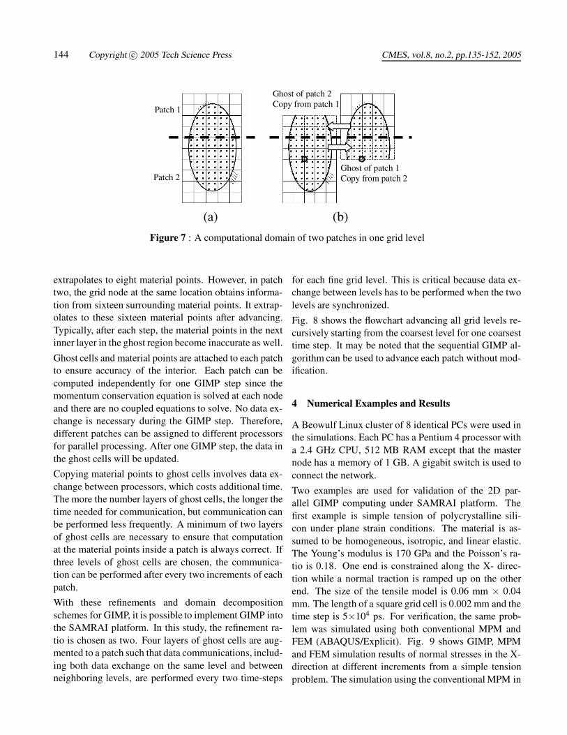
GIMP uses structured mesh, consistent with SAMRAI,so that domain decomposition is straightforward and noremeshing, in general, is necessary. Fig. 7 (a) showsa two-dimensional computational domain decomposedinto two patches separated by a horizontal dash line. Theelliptical solid object with different boundary conditionsapplied at different regions is inside this domain/grid.After discretization, there are a certain number of ma-terial points and part of the boundary in a patch, whichwill be computed individually. It may be noted that patchboundary does not have to coincide with the boundary ofthe material continuum. The patch boundary is alwayschosen to be larger than the region occupied by the mate-rial continuum so that there is extra space for the materialto deform. This will not cause any additional computa-tional burden as the GIMP computation is only carriedout on material points inside the patch. Each patch canbe processed by a single processor and the conveniencein creating patches will provide great flexibility in paral-lel processing.

Communication between two neighboring patches is re-alized through information sharing in the region over-lapped by the two patches. The overlapped regions arealso called ‘ghost’ regions, as shown in Fig. 7 (b). Theghost cells are denoted by dash lines. For ease of vi-sualization, only the ghost cells overlapped by the otherpatch are shown and the ghost cells along the other threesides of a patch are not shown. On one grid level, patchescan communicate with each other by simply copying datafrom one patch to another at the same computation time(Fig. 7 (b)). Using the material point information fromthe previous time step, and the physical boundary condi-tions, each patch is ready to advance one more time step.At this time, the material point information in the outer-most layer of the ghost cells becomes inaccurate. For in-stance, one outermost grid node in patch one, marked bythe circle, obtains information from eight material pointsbefore advancing to the next step. After advancing, it


Patch 2

Patch 1

Ghost of patch 1 Copy from patch 2

Ghost of patch 2 Copy from patch 1

(a) (b)

Figure 7 : A computational domain of two patches in one grid level

extrapolates to eight material points. However, in patchtwo, the grid node at the same location obtains informa-tion from sixteen surrounding material points. It extrap-olates to these sixteen material points after advancing.Typically, after each step, the material points in the nextinner layer in the ghost region become inaccurate as well.

Ghost cells and material points are attached to each patchto ensure accuracy of the interior. Each patch can becomputed independently for one GIMP step since themomentum conservation equation is solved at each nodeand there are no coupled equations to solve. No data ex-change is necessary during the GIMP step. Therefore,different patches can be assigned to different processorsfor parallel processing. After one GIMP step, the data inthe ghost cells will be updated.

Copying material points to ghost cells involves data ex-change between processors, which costs additional time.The more the number layers of ghost cells, the longer thetime needed for communication, but communication canbe performed less frequently. A minimum of two layersof ghost cells are necessary to ensure that computationat the material points inside a patch is always correct. Ifthree levels of ghost cells are chosen, the communica-tion can be performed after every two increments of eachpatch.

With these refinements and domain decompositionschemes for GIMP, it is possible to implement GIMP intothe SAMRAI platform. In this study, the refinement ra-tio is chosen as two. Four layers of ghost cells are aug-mented to a patch such that data communications, includ-ing both data exchange on the same level and betweenneighboring levels, are performed every two time-steps

for each fine grid level. This is critical because data ex-change between levels has to be performed when the twolevels are synchronized.

Fig. 8 shows the flowchart advancing all grid levels re-cursively starting from the coarsest level for one coarsesttime step. It may be noted that the sequential GIMP al-gorithm can be used to advance each patch without mod-ification.

4 Numerical Examples and Results

A Beowulf Linux cluster of 8 identical PCs were used inthe simulations. Each PC has a Pentium 4 processor witha 2.4 GHz CPU, 512 MB RAM except that the masternode has a memory of 1 GB. A gigabit switch is used toconnect the network.

Two examples are used for validation of the 2D par-allel GIMP computing under SAMRAI platform. Thefirst example is simple tension of polycrystalline sili-con under plane strain conditions. The material is as-sumed to be homogeneous, isotropic, and linear elastic.The Young’s modulus is 170 GPa and the Poisson’s ra-tio is 0.18. One end is constrained along the X- direc-tion while a normal traction is ramped up on the otherend. The size of the tensile model is 0.06 mm × 0.04mm. The length of a square grid cell is 0.002 mm and thetime step is 5×104 ps. For verification, the same prob-lem was simulated using both conventional MPM andFEM (ABAQUS/Explicit). Fig. 9 shows GIMP, MPMand FEM simulation results of normal stresses in the X-direction at different increments from a simple tensionproblem. The simulation using the conventional MPM in


AdvanceLevel (level_number)

Advance each patch in level by level time step

Start level_number=0

Next finer level exists AND level time > next

finer level time?

level_number = level_number+1

Data communication for level

YES

NO

End

Figure 8 : Flowchart showing advancement of grid levels recursively starting from the coarsest to the finest level inGIMP

Fig. 9 (a) shows material separation close to the free endwith severe numerical instability after 275 increments.Fig. 9 (b) and (c) show the normal stress distributionin the tensile direction and deformation after 500 incre-ments from FEM and GIMP. It may be noted that FEMresults show a stress contour plot on the deformed meshwhile the GIMP results show a discrete scattered plot ofmaterial points. These two results are in good agreementwith the difference in the maximum value being less than10%.

In the second example, indentation on the same siliconmaterial is simulated. The workpiece is subjected to apressure applied in the middle of the top surface (Fig.10 (a)) under plain strain conditions with a thickness of0.001 mm for computing the mass and forces. The mag-nitude of the pressure increases linearly with time for thefirst 1500 increments, and is then kept constant (see Fig.10 (b)). The cell size is 0.001 mm in both directions andthe time step is 20 ps for both FEM and GIMP simu-lations. Due to symmetry, only one half of the work-piece is modeled. This simulation is performed with twopatches in one uniform grid level. Two processors areused and one patch is assigned to each processor. Fig. 11

shows GIMP and FEM results of normal stresses in theY-direction at different increments. The dashed line inFig. 11 (a) is the boundary between the two patches. Fig.11 (a) and (b) are plots of normal stresses in Y-directionat 500 time increments for GIMP and FEM simulations.The difference in stress values in Fig. 11 (a) and (b) isless than 5%. It should be noted that the FEM simula-tion aborted at 1348 increments due to excessive elementdistortion. The GIMP simulation did not encounter thisproblem. Fig. 11 (c) shows the GIMP stress result af-ter 2000 increments. This demonstrates the capability ofGIMP in handling excessive distortions.

In order to validate the multi-level refinement algorithmand parallel communication, as well as the proposed con-tact algorithm, a simulation of nanoindentation with awedge indenter was conducted under 2D plane strainconditions. The workpiece is aluminum and the inden-ter is assumed to be rigid. Fig. 11 shows the indentationmodel. The area below the indenter where high stressgradients are expected is refined, as shown in Fig. 12(a). A prescribed velocity was applied on the indenter,as shown in Fig. 12 (b). The work piece dimensionsare 60 µm × 40 µm. It is fixed in the Y-direction at the


(a) Conventional MPM

(b) GIMP

(c) FEM

Figure 9 : Simulation results of tensile stress contoursfor a simple tension problem

bottom. Only half of the model is simulated because ofsymmetry. The cell sizes are 500 nm, 250 nm and 125 nmfor levels 1, 2 and 3, respectively. Each level is dividedinto four patches with approximately the same size. Themaximum indentation depth in the simulation is about450 nm. The dotted lines in Fig. 12 (a) illustrate the fourpatches in level 1. For comparison, an explicit FEM sim-ulation (using ABAQUS/Explicit) was carried out under

X

Y

(a)

Time

Pres

sure

st 8103 −×=

60 GPa

(b)

Figure 10 : Loading conditions for a simple indentationproblem

the same conditions. The FEM element size is uniformand is the same size as the finest GIMP background gridsize. In this example, the maximum indentation depth(450 nm) is relatively small compared to the finest cellsize, so that FEM simulation has not encountered exces-sive mesh distortion.

Fig. 13 shows a comparison of contours of normalstresses in the Y-direction at the maximum depth for bothFEM and parallel GIMP simulations. The axis of sym-metry of the workpiece is located at X=0.03 mm. ForFEM, the plot is the contour of nodal stresses with de-formed positions, and for GIMP, it is a discrete scatteredplot of stress at deformed material points. The area be-low the indenter with high stress gradients is refined asshown in Fig. 12 (a) for parallel GIMP computation. Theborders of grid levels 2 and 3 can barely be seen in Fig.13 (b) due to the use of high material point density. Fig.14 is a close-up view of shear stresses in which the threegrid levels are shown. Results show that the normal andshear stresses from both parallel GIMP and FEM sim-ulations agree very well. The difference of the normalstresses in the Y-direction for the material point in con-tact with the indenter tip and the stress of the FEM nodeat the same location is 4.4%. It may be noted that somenon-smoothness in the GIMP stresses around the levelboarders can be seen. This non-smoothness is caused bythe refinement and coarsening and the error associatedwith this is negligible for these simulations.

GIMP simulations using a uniform cell size of 500 nmand 125 nm were performed under the same conditions asin Fig. 12 to further verify the refinement/coarsening al-gorithm. Fig. 15 shows normal stresses in the Y-direction


(a) GIMP at 500 increments

(b) FEM at 500 increments

(c) GIMP at 2000 increments

Figure 11 : GIMP and FEM results of normal stress vari-ation in the Y-direction at different increments

V

Level 1

Level 2

3

X

Y

(a)

Time

V

20 m/s

(b)

Figure 12 : Schematic of 2D indentation showing (a)three levels of refinement and (b) the indenter velocityhistory

and shear stresses in GIMP simulations using 500 nmuniform cells. In this case the material points in contactwith the indenter are 16 times (4 times in each direction)larger than those with two levels of refinements. In gen-eral, the stress magnitudes agree with those in Fig. 13and Fig. 14.

Fig. 16 (a) shows indentation load versus depth curvesfrom FEM and GIMP with different grid sizes. FromGIMP computations, the load versus depth curves withthree levels of refinement agree very well with the re-sults from a uniform finest mesh. The load versus depthcurve from the FEM simulation with a uniform cell sizeof 125 nm under the same boundary conditions is plot-ted for comparison. It can be seen from Fig. 16 (a) thatthe trend of the load versus depth plots from FEM andGIMP simulations are similar. The difference in inden-tation load at the end of loading, which corresponds to450 nm of indentation depth, is 5.9% between FEM andGIMP with 3 grid levels. When the depth is less than100 nm, there is only one material point in contact withthe rigid indenter. The assumption of constant pressurecauses large differences under this circumstance. How-


(a) FEM

(b) GIMP

Figure 13 : Comparison of normal stresses in Y-directionfrom FEM and GIMP

ever, if the GIMP cell size is further refined to 62.5 nmand the size of the material point is 31.25 nm, the differ-ence between GIMP and FEM becomes smaller, as canbe seen in Fig. 16 (b).

Other simulations were conducted for the same problem

(a) FEM

(b) GIMP

Figure 14 : Comparison of shear stresses from FEM andGIMP

with three levels of refinement using different number ofprocessors to test the efficiency of parallel computing.The number of patches at each level is the same as thenumber of processors and the size of each patch is ap-proximately the same. The resultant stress distributionand indentation load versus depth plots are the same asthe previous results. The average time per computationalstep is 7.14 sec. when one processor is used and is re-duced to 4.26, 3.40, 2.18 sec., respectively when two,three, and four processors are used. When four proces-sors are used, the CPU time per step is only 30.5% ofthat of one processor. This gives a speed-up by a factor


(a) Normal Stress

(b) Shear Stress

Figure 15 : Normal and shear stresses of GIMP simula-tions with a uniform cell size of 500 nm

of 3.28. In the ideal case without communication over-head, the speed-up would be 4. The reduction in speed-

up from the ideal number is because of the time involvedin data communication between processors. It has beenobserved that the refinement and coarsening algorithmconsume most of the communication time. Moreover,in refinement and coarsening, most of the time is takento search for the corresponding material point in anothergrid level. This portion of the computational time can bereduced, if improved searching algorithm or more opti-mized algorithm for the storage of material points can beimplemented.

The manual refinement for the indentation problem is ad-equate since the region of high stress gradient is knownto occur below the indenter. The finest level covers theindenter and part of the specimen. With the same ini-tial condition, the results at the finest level is identical tothe results in the same area if a uniform fine mesh is usedfor the entire domain that requires much longer computa-tional time. The computational load of each processor isbalanced statically by assigning approximately the samenumber of material points to each processor. Dynamicload balance is supported by SAMRAI and can poten-tially improve the efficiency of the simulation.

To demonstrate the capability of the algorithm developedin this investigation for multiscale simulation, an indenta-tion model with multiple length scales is simulated witheight processors. The dimensions of the workpiece are0.25 mm × 0.125 mm. Initially, the velocity of the in-denter increases from 0 to 150 m/s linearly with timeand is then kept constant. Five successive levels of re-finement are used in this simulation. The smallest ma-terial point represents an area of 64 nm × 64 nm, andthe largest material point covers an area of 1 µm × 1µm. Each level is divided into 8 equal-sized patches forbest load balance. Since the contact surface can evolveinto several patches, a parallel solver is implemented tosolve Eq. (11) to find the contact pressure based on thePortable, Extensible Toolkit for Scientific Computation(PETSc). An aluminum workpiece is chosen with theYoung’s modulus and Poisson’s ratio of 70 GPa and 0.33,respectively. The maximum indentation depth was 9.8µm in this simulation (i.e., 153 times the size of the finestmaterial point). It took nine hours to simulate this prob-lem with eight processors. Fig. 17 (a) gives the normalstress distributions and Fig. 17 (b) shows normal stressdistribution for the finest two levels. The relative largedeformation in this multiscale nanoindentation problemcould not be handled by FEM due to excessive distortion


0

1

2

3

4

5

6

0 100 200 300 400 500

Depth (nm)

Lo

ad (

mN

)

GIMP-coarse (500 nm)

GIMP-fine (125 nm)

GIMP-3 levels FEM-fine (125 nm)

(a) FEM

0

0.5

1

1.5

2

2.5

0 40 80 120 160

Depth (nm )

Load (mN)

GIM P-500 nm

GIM P-125 nm

GIM P-62.5 nm

FEM -62.5 nm

(b) GIMP

Figure 16 : Indentation load versus depth curves fromFEM and GIMP with different grid sizes

in the FEM mesh. However, the parallel GIMP code wasable to complete the entire loading/unloading processeswithout any difficulty. This example shows clearly theadvantage of GIMP for multiscale simulations over FEM.

5 Conclusions

The following are specific conclusions based on the re-sults of this investigation:

1. A 2D generalized interpolation material point (GIMP)method has been implemented to address problems, suchas particle flying-off and alternating stress sign associ-ated with conventional MPM in case of relatively large

(a) FEM

(b) GIMP

Figure 17 : Multiscale simulation of nanoindentationwith five levels of refinement

deformation.

2. To conduct multiple length scale simulations, aparallel computing scheme has been presented usingGIMP under SAMRAI parallel computing environmentin which multi-level grids are used for spatial and tem-poral refinements.

3. A refinement/coarsening algorithm, based on materialpoints of GIMP in two grid levels, has been developed


for communication between neighboring grid levels ofdifferent refinements. With increase in the refinementlevels, as well as decrease in the time step increments,the computational accuracy is greatly improved in the re-gion of interest while the overall computational time isreduced. The computation at each grid level is performedrecursively to ensure that the refinement and coarseningare performed when the two neighboring levels are syn-chronized.

4. 2D MPM and GIMP were applied to simple ten-sion and indentation problems to validate the GIMP al-gorithm. GIMP results agree very well with FEM resultsfor these two examples provided that the deformationsare small. The noise and instability problems present inconventional MPM are not observed in the GIMP simu-lations.

5. As the deformation is increased, GIMP continued toexecute while FEM aborted due to element distortion.Also GIMP results are stable. Thus GIMP is able to han-dle relatively large deformation problems.

6. For the nanoindentation problem, a GIMP algorithmfor the contact between a rigid indenter and a deformableworkpiece was developed. A reasonably good agreementbetween GIMP and FEM results was reached, validatingthe contact algorithm presented in this investigation.

7. Another nanoindentation example with multiplelength scales from a few nanometers to sub-millimeterswas simulated and numerical results validated the paral-lel GIMP computing with the use of SAMRAI.

Acknowledgement: The work was supported by agrant from the Air Force Office of Scientific Research(AFOSR) through a DEPSCoR grant (No. F49620-03-1-0281). The authors would like to thank Dr. Craig S. Hart-ley, Program Manager for Metallic Materials Program atAFOSR for his interest and support of this work. Theauthors also acknowledge Dr. Scott Bardenhagen for hisintroduction to the GIMP algorithm and valuable com-ments, and Dr. John A. Nairn for providing the 2D MPMcode.

Disclaimer

This document was prepared as an account of work spon-sored by an agency of the United States Government.Neither the United States Government nor the Univer-sity of California nor any of their employees, makes any

warranty, express or implied, or assumes any legal li-ability or responsibility for the accuracy, completeness,or usefulness of any information, apparatus, product, orprocess disclosed, or represents that its use would not in-fringe privately owned rights. Reference herein to anyspecific commercial product, process, or service by tradename, trademark, manufacturer, or otherwise, does notnecessarily constitute or imply its endorsement, recom-mendation, or favoring by the United States Governmentor the University of California. The views and opinionsof authors expressed herein do not necessarily state orreflect those of the United States Government or the Uni-versity of California, and shall not be used for advertisingor product endorsement purposes.

References

Atluri, S.N.; Shen, S. (2002): The meshless localPetrov-Galerkin (MLPG) method: a simple & less-costlyalternative to the finite element and boundary elementmethods.CMES: Computer Modeling in Engineering &Sciences, vol. 3, no. 1, pp. 11-51.

Bardenhagen, S.G. (2002): Energy conservation errorin the material point method for solid mechanics. Journalof Computational Physics, vol. 180, pp. 383-403.

Bardenhagen, S.G.; Kober, E.M. (2004): The gener-alized interpolation material point method.CMES: Com-puter Modeling in Engineering & Sciences, vol. 5, no. 6,pp. 477-496.

Berger, M.J.; Oliger, J. (1984): Adaptive mesh refine-ment for hyperbolic partial differential equations. Jour-nal of Computational Physics, vol. 82, pp. 484-512.

Hornung, R.D.; Kohn, S.R. (2002): Managing applica-tion complexity in the SAMRAI object-oriented frame-work. Concurrency and Computation: Practice and Ex-perience, vol. 14, pp. 347-368.

Horstemeyer, M.F.; Baskes, M.I.; Prantil, V.C.;Philliber, J.; Vonderheide, S. (2003): A multiscale anal-ysis of fixed-end simple shear using molecular dynamics,crystal plasticity, and a macroscopic internal state vari-able theory. Modelling and Simulation in Materials Sci-ence and Engineering, vol. 11, pp. 265-286l.

Hsien, S.H. (1997): Evaluation of automatic domain par-titioning algorithms for parallel finite element analysis.International Journal for Numerical Methods in Engi-neering, vol. 40, pp. 1025-1051.


Hu, W.; Chen, Z. (2003): A multi-mesh MPM for sim-ulating the meshing process of spur gears. Computers &Structures, vol. 81, pp. 1991-2002.

Kalia, R.K.; Nakano, A.; Greenwell, D.L.; Vashishta,P. (1993): Parallel algorithms for molecular dynamicssimulations on distributed memory MIMD machines. Su-percomputer, vol. 54, pp. 11-25.

Komanduri, R.; Lu, H.; Roy, S.; Wang, B.; Raff, L.M.(2004): Multiscale modeling and simulation for materi-als processing. Proceedings of the AFOSR Metallic Ma-terials (2306 AX) Grantees Meeting, VA, USA.

Mackerle, J. (2003): FEM and BEM parallel process-ing: theory and applications-a bibliography. EngineeringComputation, vol. 20, no. 4, pp. 436-484.

Oden, J.T.; Pires, E.B. (1983): Numerical analysis ofcertain contact problems in elasticity with non-classicalfriction laws. Computers & Structures, vol. 16, no. 1-4,pp. 481-485.

Shen, S.; Atluri, S. N. (2004a): Computational nano-mechanics and multi-scale simulation. CMC: Comput-ers, Materials, & Continua, vol. 1, no. 1, pp. 59-90.

Shen, S.; Atluri, S. N. (2004b): Atomic-level stress cal-culation and continuum-molecular system equivalence.CMES: Computer Modeling in Engineering & Sciences,vol. 6, no. 1, pp. 91-104.

Shen, S.; Atluri, S. N. (2005): A tangent stiffnessMLPG method for atom/continuum multiscale simula-tion. CMES: Computer Modeling in Engineering & Sci-ences, vol. 7, no. 1, pp. 49-67.

Sulsky, D.; Zhou, S.J.; Schreyer, H.L. (1995): Appli-cation of a particle-in-cell method to solid mechanics.Computer Physics Communications, vol. 87, pp. 236-252.

Sulsky, D.; Schreyer, H.L. (1996): Axisymmetric formof the material point method with applications to up-setting and Taylor impact problems. Comput. MethodsAppl. Mech. Eng., vol. 139, pp. 409-429.

Tan, H.; Nairn, J.A. (2002): Hierarchical, adaptive, ma-terial point method for dynamic energy release rate cal-culations. Computer Methods in Applied Mechanics andEngineering, vol. 191, pp. 2095-2109.

Tewary, V. K.; Read D. T. (2004): Integrated Green’sfunction molecular dynamics method for multiscalemodeling of nanostructures: application to Au nanois-land in Cu. CMES: Computer Modeling in Engineering

& Sciences, vol. 6, no. 4, pp. 359-371.

Wissink, A.M.; Hysom, D.; Hornung, R.D. (2003):Enhancing scalability of parallel structured AMRA cal-culations. Proc. 17th ACM International Conference onSupercomputing (ICS03), San Francisco, CA, pp. 336-347.

Zhong, Z.H. (1993): Finite Element Procedures forContact-Impact Problems, Oxford University Press, NewYork.

Multiscale Simulations Using Generalized Interpolation Material Point ... · ized interpolation material point (GIMP) method, Bar-denhagen and Kober (2004), ... ρw·bsdΩ, (1) where

Documents