Multiscale simulation of complex fluid flow using … · Multiscale simulation of complex fluid flow using coupled models Rafael Delgado Buscalioni Universidad de Educaci´on

Multiscale simulation of complex fluid flowusing coupled models

Rafael Delgado Buscalioni

Universidad de Educacion a DistanciaMadrid

collaboration with:

Gianni De Fabritiis (University College London)

Jens Harting (Stuttgart University). HPC-Europa funding @ HLRS

1

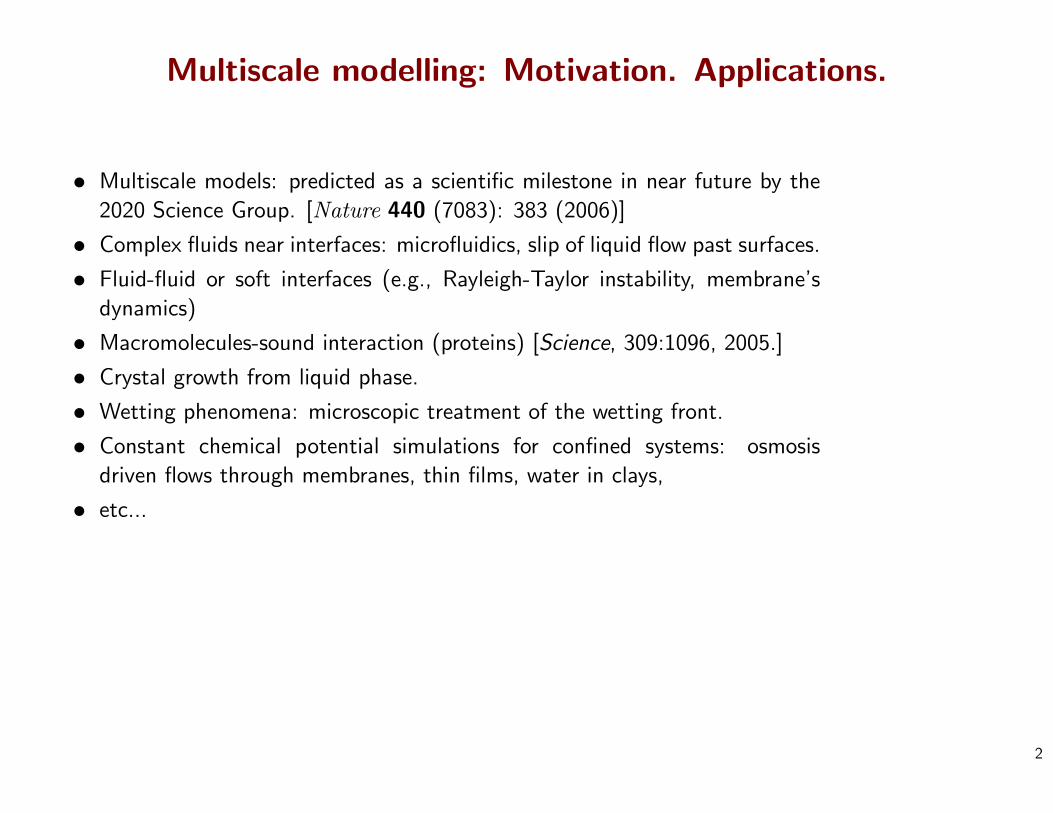
Multiscale modelling: Motivation. Applications.

• Multiscale models: predicted as a scientific milestone in near future by the

2020 Science Group. [Nature 440 (7083): 383 (2006)]

• Complex fluids near interfaces: microfluidics, slip of liquid flow past surfaces.

• Fluid-fluid or soft interfaces (e.g., Rayleigh-Taylor instability, membrane’s

dynamics)

• Macromolecules-sound interaction (proteins) [Science, 309:1096, 2005.]

• Crystal growth from liquid phase.

• Wetting phenomena: microscopic treatment of the wetting front.

• Constant chemical potential simulations for confined systems: osmosis

driven flows through membranes, thin films, water in clays,

• etc...

2

Mulstiscale techniques

the art of inventing a wise...

TrickAstuceTruco

ScherzzoZaubern

τεχνασµα = technasma

3

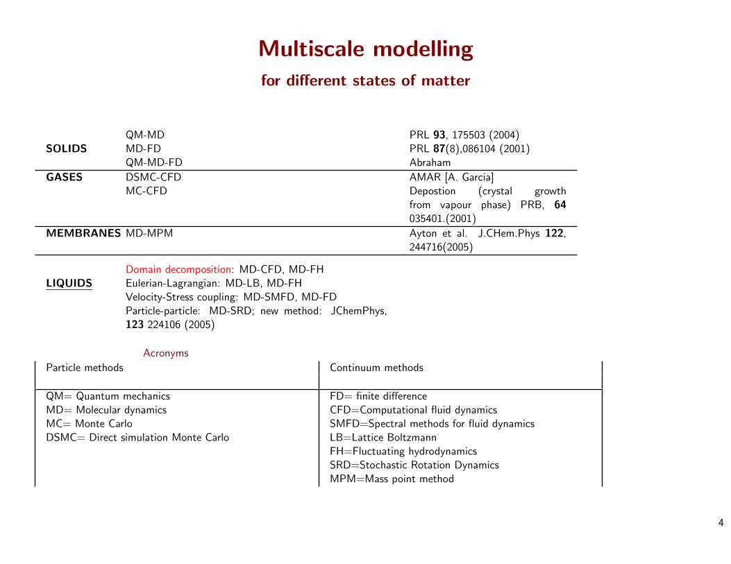
Multiscale modellingfor different states of matter

QM-MD PRL 93, 175503 (2004)SOLIDS MD-FD PRL 87(8),086104 (2001)

QM-MD-FD Abraham

GASES DSMC-CFD AMAR [A. Garcia]MC-CFD Depostion (crystal growth

from vapour phase) PRB, 64035401.(2001)

MEMBRANES MD-MPM Ayton et al. J.CHem.Phys 122,244716(2005)

Domain decomposition: MD-CFD, MD-FHLIQUIDS Eulerian-Lagrangian: MD-LB, MD-FH

Velocity-Stress coupling: MD-SMFD, MD-FDParticle-particle: MD-SRD; new method: JChemPhys,123 224106 (2005)

Acronyms

Particle methods Continuum methods

QM= Quantum mechanicsMD= Molecular dynamicsMC= Monte CarloDSMC= Direct simulation Monte Carlo

FD= finite differenceCFD=Computational fluid dynamicsSMFD=Spectral methods for fluid dynamicsLB=Lattice BoltzmannFH=Fluctuating hydrodynamicsSRD=Stochastic Rotation DynamicsMPM=Mass point method

4

Multiscale modelling:Complications with liquids

• Large intermolecular potential energy, cohesion.

• Large mobility. Open systems, particle insertion, etc...

• Fluctuations are important at molecular scales:

– Fluctuating-deterministic coupling (how to reduce effect of particle fluctuations in the continuum

region).

– Use of stochastic fluid models: fluctuating hydrodynamics

• Soft matter: self-assembly process (eg,. water+surfactants)

• Wide gap between time-scales: time decoupling. Coarse-grained models with specific molecular properties.

5

Multiscale modelling of liquids: different scenarios.

Domain decomposition

Eulerian-Lagrangianhybrid:

Stokes force couplingVelocity-Stressmesh coupling

Ccontinuum fluid dynamics

P

MD simulations in periodic boxes (MD nodes) evaluate the local stress

for the Continuum solver.

The Continuum field provides the local velocity gradient imposed at each MD node.

Particles: MD Continuum: LB or FH.

Fluctuations in C model needed. Explicit solvent-solute interaction

interfases, surfaces,single macromole-fluid interaction

Molecularregion

Bestmethod

localized in bulk concentrated solution or melt

hydrodynamics of semidilute solutions

MD

Highly non-Newtonian fluid flow

applications

LB

6

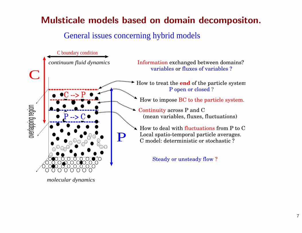
Mulsticale models based on domain decompositon.

General issues concerning hybrid models

continuum fluid dynamics

molecular dynamics

C

C boundary condition

P

How to impose BC to the particle system.

How to treat the end of the particle systemP open or closed ?

Continuity across P and C (mean variables, fluxes, fluctuations)

How to deal with fluctuations from P to C ? Local spatio-temporal particle averages. C model: deterministic or stochastic ?

Information exchanged between domains? variables or fluxes of variables ?

P --> C

C --> P

Steady or unsteady flow ?

overlap

ping re

gion

7

Hybrids based on domain decomposition

ModelInformationexchanged

P: open or closedBoundaryconditionsimposed to P

.Continuity

C Deterministicor Stochastic

Steady orUnsteady

Schwartzcoupling

Variables:transversal velocity(shear)

closed:shear,incompressiblefluids)

Maxwell daemonto velocity

Variable (YES),Fluxes (NO),Fluctuations (NO)

Deterministic Steady

Fluxcoulping

Fluxes ofconservedquantities (mass,momentum,energy)

open:sound+energy

External forces Variables (YES)...(via relaxation)Fluxes (YES)Fluctuations (YES)

Stochastic orDeterministic

Unsteady

8

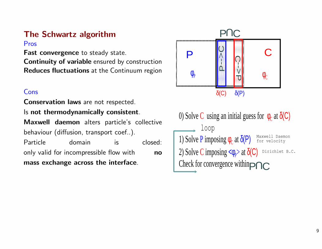
The Schwartz algorithmPros

Fast convergence to steady state.

Continuity of variable ensured by construction

Reduces fluctuations at the Continuum region

Cons

Conservation laws are not respected.

Is not thermodynamically consistent.

Maxwell daemon alters particle’s collective

behaviour (diffusion, transport coef..).

Particle domain is closed:

only valid for incompressible flow with no

mass exchange across the interface.

P C

CP

UC

P--

>

PC

-->δ(C) δ(P)

0) Solve C using an initial guess for φC at δ(C) loop1) Solve P imposing φC at δ(P) 2) Solve C imposing <φP> at δ(C)Check for convergence within CP

U

Dirichlet B.C.

Maxwell Daemon for velocity

φP φC

9

The Flux coupling scheme

PCHp

HcJ

Hc

φ_CJ

Hc

φ_P=

JHp

φ_CJ

Hp

φ_P=

overlapping region

C-P P--C

Flux continuity

Previous flux based schemes

Total system : ??Continuum sudomain: COverlapping region: ? Particle subdomain: P

Flekkoy et al.RDB & P. Coveney

Nie, et al.

The total system was not well defined

10

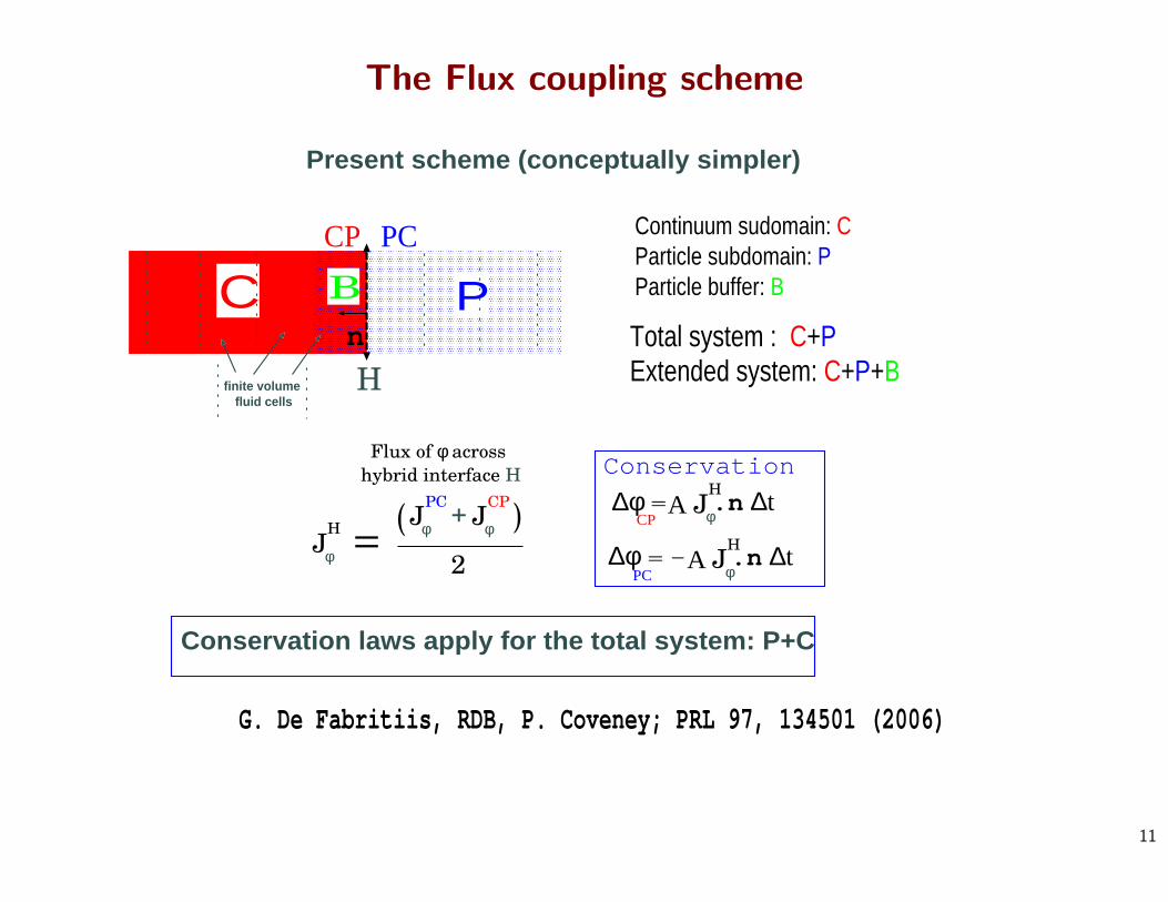
The Flux coupling scheme

Present scheme (conceptually simpler)

Total system : C+PExtended system: C+P+B

Continuum sudomain: CParticle subdomain: PParticle buffer: B

G. De Fabritiis, RDB, P. Coveney; PRL 97, 134501 (2006)

Conservation laws apply for the total system: P+C

B

H

PCCP

nC P

finite volume fluid cells

Flux of φ across hybrid interface H

JPC

φ=JH

φ

JCP

φ+( )2

JH

φA ∆t∆φCP

.n=

∆φPC= J

H

φA ∆t.n-

Conservation

11

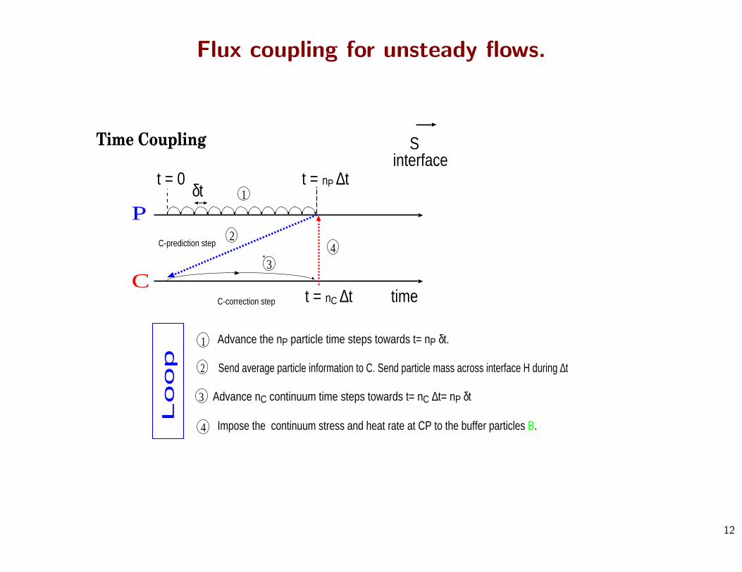
Flux coupling for unsteady flows.

1

42

3

P

Ctime

t = 0 t = nP ∆tδt

C-prediction step

C-correction step

Time Coupling Sinterface

t = nC ∆t

4 Impose the continuum stress and heat rate at CP to the buffer particles B.

2 Send average particle information to C. Send particle mass across interface H during ∆t

1 Advance the nP particle time steps towards t= nP δt.

3 Advance nC continuum time steps towards t= nC ∆t= nP δt

Loop

12

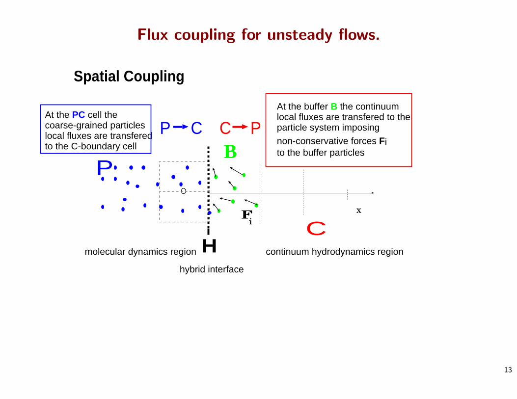
Flux coupling for unsteady flows.

Spatial Coupling

At the PC cell the coarse-grained particles local fluxes are transfered to the C-boundary cell

P C C PAt the buffer B the continuum local fluxes are transfered to the particle system imposing non-conservative forces Fi to the buffer particles

Cx

B

Hhybrid interface

molecular dynamics region continuum hydrodynamics region

P

Fi

13

The particle buffer B

• Objective: Impose momentum and energy (C → P )

• Requirement: Control the buffer’s mass MB = m NB

• Method: The buffer is always filled with particles via a simplerelaxation algorithm.

dNB

dt=

1τB

(αNCP −NB)

with τB ' [10 − 100]fs (faster than any hydrodynamic time)and α ' 0.75.

• Particle evaporating out of the buffer B are removed. If∆NB > 0, particles are inserted using the usher algorithm(insertion energy equal to the mean energy/particle)

14

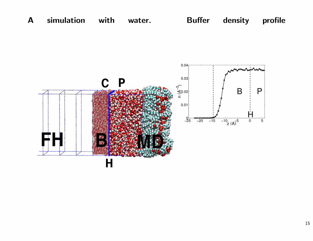
A simulation with water. Buffer density profile

−25 −20 −15 −10 −5 0 50

0.01

0.02

0.03

0.04

n (A

−3)

z (A)

B P

H

15

Fast particle insertionwith controlled release of potential energyusher J. Chem. Phys 119, 978 (2003); J. Chem. Phys. 121, 12139 (2004)

(water)

-15 -10 -5 0 5 1010

1

102

103

104

105

10 6

107

E (Kcal/mol)

Number of insertion trials (or iterations) required to insert a water molecule in water, at a potential energy E

Random insertion

USHER algorithmfor water

water chemical potential at 300Κ

average potential energy per molecule at 300Κ

numb

er of

energ

y eva

luatio

ns

0.4 0.5 0.6 0.7 0.8 0.9 1ρ [σLJ

-3]

2

2.5

3

3.5

4

Tot

al e

nerg

y pe

r pa

rtic

le [ε

LJ]

0.3 0.4 0.5 0.6 0.7 0.8 0.9 1ρ [σLJ

-3]

0

5

10

15

20

25

30

Pres

sure

[ε L

J/σL

J3 ]

0.3 0.4 0.5 0.6 0.7 0.8 0.9 1ρ [σLJ

-3]

2

2.5

3

3.5

4

4.5

5

Tem

pera

ture

[εL

J/kB]

0.3 0.4 0.5 0.6 0.7 0.8 0.9 1ρ [σLJ

-3]

-4

-3.5

-3

-2.5

-2

-1.5

-1

Exc

ess

ener

gy p

er p

artic

le [ε

LJ]

< ε > = 0.001

Density increases with time, dρ/dt = 0.01 σ-3τ-1

Insertion process at constant energy per particledashed line thermodynamic analytical solution (Lennard-Jones fluid)

16

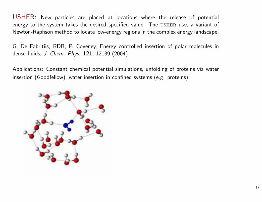
USHER: New particles are placed at locations where the release of potential

energy to the system takes the desired specified value. The usher uses a variant of

Newton-Raphson method to locate low-energy regions in the complex energy landscape.

G. De Fabritiis, RDB, P. Coveney, Energy controlled insertion of polar molecules in

dense fluids, J. Chem. Phys. 121, 12139 (2004)

Applications: Constant chemical potential simulations, unfolding of proteins via water

insertion (Goodfellow), water insertion in confined systems (e.g. proteins).

17

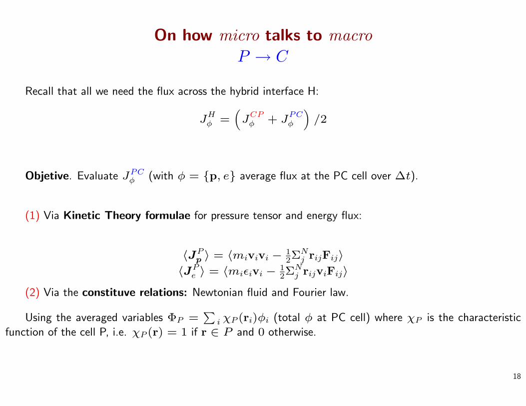
On how micro talks to macroP → C

Recall that all we need the flux across the hybrid interface H:

JHφ =

(J

CPφ + J

PCφ

)/2

Objetive. Evaluate JPCφ (with φ = {p, e} average flux at the PC cell over ∆t).

(1) Via Kinetic Theory formulae for pressure tensor and energy flux:

〈JPp 〉 = 〈mivivi − 1

2ΣNj rijFij〉

〈JPe 〉 = 〈miεivi − 1

2ΣNj rijviFij〉

(2) Via the constituve relations: Newtonian fluid and Fourier law.

Using the averaged variables ΦP =∑

i χP (ri)φi (total φ at PC cell) where χP is the characteristic

function of the cell P, i.e. χP (r) = 1 if r ∈ P and 0 otherwise.

18

On how macro talks to micro:C → P

[Flekkoy, RDB, Coveney, Phys. Rev. E, 72, 026703 (2005)]

Objective: To impose into the P system the desired (exact) energy and momentum flux across the

interface H: that is JHe and JH

p , respectively.

Method: By adding an external force Fi to the particles at the B reservoir.

Momentum and energy added to P+ B over one (long) time step dt = ∆t

Momentum JpA∆t =∑

i∈CP Fi∆t +∑

i′ ∆(mvi′)

Energy JeA∆t︸ ︷︷ ︸Total input

=∑i∈B

Fi · vi∆t︸ ︷︷ ︸External force

+∑

i′∆εi′︸ ︷︷ ︸

Particle insertion/removal

where A is the H-interface area and the index i′ runs only over added/removed particles during ∆t.

19

On how macro talks to micro: C → P (cont.)

Decomposition of the external particle force: Fi = F + F′i

The mean value 〈Fi〉 = F provides the desired input of momentum

F =A

NB

jp where jp ≡ Jp −∑

i′ ∆(mvi′)

A dt. (1)

The fluctuating part F′i provides the desired energy input via dissipative work

(note that F′i gives no net momentum input because

∑NBi=1 F′

i = 0).

F′i =

Av′i∑NBi=1 v′2i

[je − jp · 〈v〉

]with je ≡ Je −

∑i′ ∆εi′

Adt. (2)

Under equilibrium, the second law of thermodynamics is respected and the particle system behaveslike an open system at constant chemical potential, µ = µ(P C, T C), given by the pressure P C andtemperature T C imposed at the B reservoir.

20

Molecular dynamics at various ensembles

[Flekkoy, RDB, Coveney, Phys. Rev. E, 72, 026703 (2005)]

Amount of heat and work into the MD system is exactly controlled.

Enabling

• Grand-canonical ensemble. µVT. Where µ = µ(pC, T C) is the chemical potential at the reservoir B.

• Isobaric ensemble NPT. Jp = pn.

• Constant enthalpy HPT. JHe = M〈v〉·F and ∆N = 0. ∆E+p∆V = ∆H = 0. (Joule-Thompson)

• Constant heat flux. Je = cte. (growth of solid phase -ice-, heat exchange at complex surfaces.)

with further benefits

• The system comunicates with the exterior at its boundaries (B), as a real system does.

• Dynamic properties are measurable. Inside the interest region, MD is not altered by any artifact

(thermostat, manostat, etc...).

21

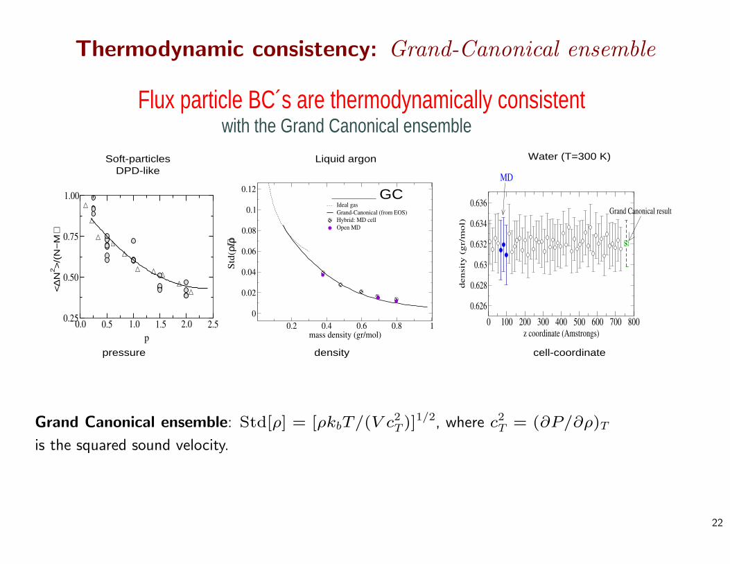
Thermodynamic consistency: Grand-Canonical ensemble

0.0 0.5 1.0 1.5 2.0 2.5p

0.25

0.50

0.75

1.00

<∆

Ν2 >

/(Ν

−Μ

)

0.2 0.4 0.6 0.8 1mass density (gr/mol)

0

0.02

0.04

0.06

0.08

0.1

0.12

Std(

ρ)/ρ

Ideal gasGrand-Canonical (from EOS)Hybrid: MD cellOpen MD

0 100 200 300 400 500 600 700 800z coordinate (Amstrongs)

0.626

0.628

0.63

0.632

0.634

0.636

dens

ity

(gr/

mol

)

Grand Canonical result

MD

Soft-particlesDPD-like

Liquid argon Water (T=300 K)

pressure density cell-coordinate

Flux particle BC´s are thermodynamically consistent

GC

with the Grand Canonical ensemble

Grand Canonical ensemble: Std[ρ] = [ρkbT/(V c2T )]1/2, where c2

T = (∂P/∂ρ)T

is the squared sound velocity.

22

Variable continuity: On how macro and micro finally agree.Important question: In case of disagreement, who is right, P or C?

C is right P is right

Authors Nie et al Present work (and Garcia DSMC-CFD)

velocitycontinuity: (a) Contraint particle dynamics (b) Relaxation term in NS eqs. for CP cell

mass flux imposed by C to P Given by the particle flux across H

(ruled by pressure)

(a) Constrained dynamics: [Thompson and O’Connel, PRE, (1995); Nie et al. J. Fluid Mech. (2004)].

dx2i

dt= Fi/m +

1

τr

(v

CCP − 〈v〉P

CP

)(b) Relaxation of first C cell: [RDB, Flekkoy, P.Coveney, EuroPhys. Lett. (2005)]

[ρv]CCP

dt= NS +

1

τr

(〈[ρv]

P〉CP − [ρv]CCP

)Note: Constraining the particle dynamics affects the particle collective properties. It also destroys energy

balance. Relaxation of the Continuum cell (CP) is simple and efficient, τr << τhydro.

23

Fluctuations are important at the nanometer and micron scales

MD Stress fluctuations are consistent withLandau Theory for fluctuating hydrodynamics.

Numerical Theoretical

Fluid VPC T η Var[jPxy] Landau theory or (Zwanzig and Mountain, 1965)

WCA 81 1 1.75 0.51 0.60

WCA 173 1 1.75 0.40 0.41

WCA 138 1 1.75 0.33 0.38

WCA 338 1 1.75 0.25 0.24

WCA 2778 1 1.75 0.08 0.06

WCA 2778 1 1.75 0.04 0.03

LJ 121.5 4.0 2.12 1.09 1.08 (1.19)

LJ 121.5 2.0 1.90 0.66 0.72 (0.71)

LJ 121.5 1.0 1.75 0.39 0.49 (0.43)

Density ρ = 0.8 (all in LJ units)

24

Fluctuations are important at the nanometer and micron scales

Thus it is possible to couple

molecular dynamics with fluctuating hydrodynamics

MD-FH hybridFor liquid phase: water, argon...

25

Fluctuating hydrodynamics solver based on Landau Theory

Conservative stochastic equations, solved using an Eulerian Finite Volume method with an

explicit time integration scheme (Euler).

∂

∂t

Variables, Φ

ρρuρe

= −∇

Fluxes, J

ρuρuu + Π

ρue + Π : u + Q

−∇

Fluctuations, J

0

Π

Q

massmomentum

energy

(3)

Finite Volume: space is discretized using control cells of volume Vc

ddt

∫Vk

φ(x, t)dx =∑

l

AklJφkl · ekl,

26

[G. De Fabritiis,RDB,preprint, 2006; GDF, Mar Serrano, RDB, preprint, 2006 ] The value of any quantity at the surface kl is approximated asφkl = (φl + φk)/2. We then obtain the following formal stochastic equations,

dMtk =

∑l

gkl · eklAkldt, (4)

dPtk =

∑l

[Πl2· ekl + gkl · eklvkl

]Akldt + dPt

k, (5)

where gkl = 12(ρk + ρl)

12(vk + vl).

Discretization of the gradients satisfying the fluctuation-dissipation theorem.

Παβk

=ηkVk

∑l

[1

2Akl(e

αklv

βl

+ eβkl

vαl )−

δαβ

DAkle

γkl

vγl

],

πk =ζkVk

∑l

1

2Akle

βkl

vβl

. (6)

The fluctuating component of the momentum is

dPtk =

∑l

1

2Akl

(4kbTl

ηlVl

)1/2

dWSl · ekl +

∑l

1

2Akl

(2DkbTl

ζlVl

)1/2tr[dWl]

Dekl, (7)

where dWSl = (dWl + dWT

l )/2− tr[dWl]/D1 is a traceless symmetric random matrix and dWl is a D × D matrix (D = 3 in three dimensions)

of independent Wiener increments satisfying < dWα,βk

dWγ,δl

>= δk,lδα,γδβ,δδt.

27

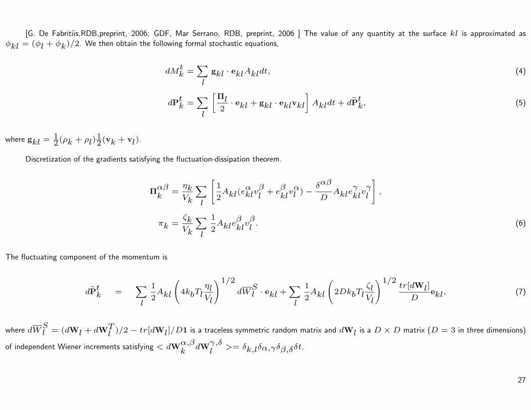
Hybrid MD-FH at equilibrium

0 100 200 300 400 500 600 700 800z coordinate (Amstrongs)

0.626

0.628

0.63

0.632

0.634

0.636

densit

y (

gr/

mol)

Grand Canonical resultMD cells

FH cells (white)

Thermal fluctuations thresholds

0.1 1

0.0001

0.001

Erro

r per

mas

s

10 100

0.0001

0.001

Std(P)/M

Std(M)/M

τ−1/2

(transversal)

(longitudinal)

Mass

τ (ps)

Py

Pz

Global mass & momentum conservation(isothermal case, water, T=300 K)

Density-pressure consistency(isothermal case, water, T=300 K)

isothermal simulations: DPD thermostat for MD [(Dunweg et al.)]

28

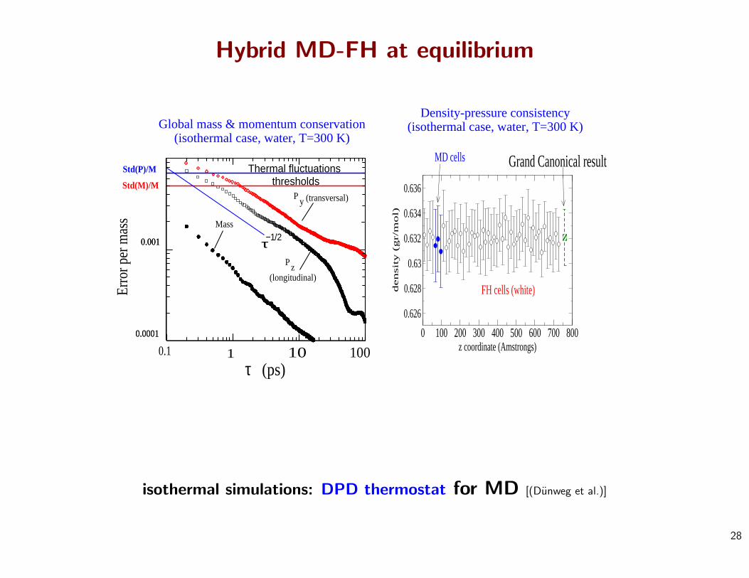
Hybrid MD-FH under non-equilibrium: unsteady shear flow

0 50 100 150 200z (Amstrongs)

-0.01

0

0.01

0.02

0.03

0.04

0.05

0.06

x-ve

loci

ty (N

AM

D u

nits) HYDRO

HYBRID

y = -0.009043 + 0.0003012 z

29

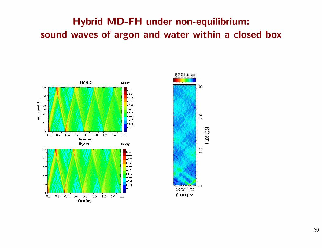
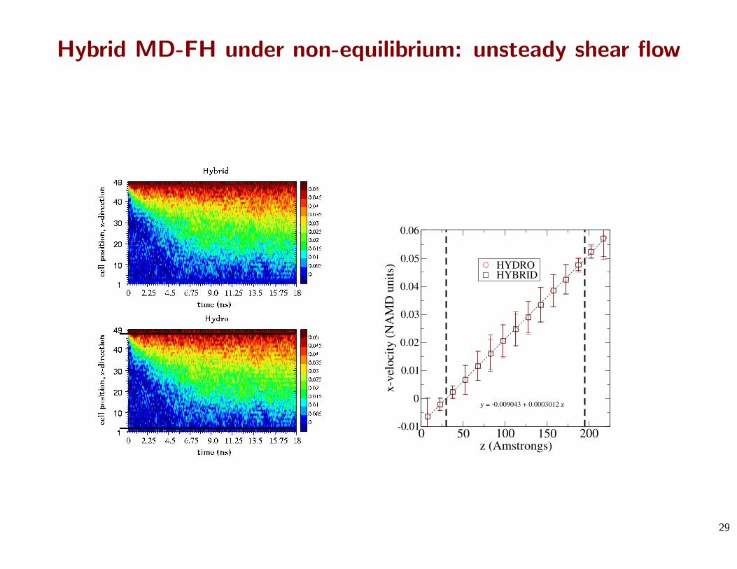
Hybrid MD-FH under non-equilibrium:sound waves of argon and water within a closed box

30

0.625

0.63

0.635

0.64

0.645

0.65

0.655

0 20 40 60 80

100

200

300

400

500

600

700

t (ps)

z (A

)

MD

FH

FH

g/mol/A3

(a)

31

32

Water wave reflecting against a DMPC monolayer

33

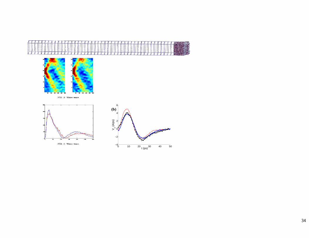
0 10 20 30 40 50−4

−2

0

2

4

6

t (ps)

Vz (

A/p

s)(b)

34

Conclusions

• Overview of the multiscale methods for liquid phase.

• Previous hybrid models for liquid phase were not mature enough for many problems: restricted to shear

flow, deterministic continuum and Lennard Jones atoms:

• In this work we generalize the hybrid scheme for liquids and include:

– Sound and energy (mass transport)

– fluctuating hydrodynamics (FH)

– Realistic MD potentials: water as solvent, complex molecules as solutes (using MINDY).

The model

• Respect conservation laws by construction (flux-exchange).

• MD is an open system and its mass fluctuation is consistent with the Grand-Canonical ensemble.

• MD velocity and pressure fluctuations are consitent with FH.

• Applied problem (1): Slippage of water over hydrophobic surfaces (DMPC monolayer); effect of

including small ammount of dissolved argon.

• Applied problem (2): Macromolecule sound interaction (resonance under high-frequency perturbation).

35