Multiscale Morse theory for science discovery

This content has been downloaded from IOPscience. Please scroll down to see the full text.

Download details:

IP Address: 54.224.135.207

This content was downloaded on 04/06/2016 at 00:16

Please note that terms and conditions apply.

Multiscale Morse theory for science discovery

View the table of contents for this issue, or go to the journal homepage for more

2008 J. Phys.: Conf. Ser. 125 012098

(http://iopscience.iop.org/1742-6596/125/1/012098)

Home Search Collections Journals About Contact us My IOPscience

Multiscale Morse theory for science ciscovery

Valerio Pascucci1 and Ajith Mascarenhas2

1 Scientific Computing and Imaging Institute, School of Computing, University of Utah, SaltLake City, UT 84112, USA2 Center for Applied Scientific Computing, Lawrence Livermore National Laboratory,Livermore, CA 94551, USA

E-mail: [email protected]

Abstract. Computational scientists employ increasingly powerful parallel supercomputers tomodel and simulate fundamental physical phenomena. These simulations typically producemassive amounts of data easily running into terabytes and petabytes in the near future. Thefuture ability of scientists to analyze such data, validate their models, and understand thephysics depends on the development of new mathematical frameworks and software tools thatcan tackle this unprecedented complexity in feature characterization and extraction problems.We present recent advances in Morse theory and its use in the development of robust dataanalysis tools. We demonstrate its practical use in the analysis of two large scale scientificsimulations: (i) a direct numerical simulation and a large eddy simulation of the mixing layer ina hydrodynamic instability and (ii) an atomistic simulation of a porous medium under impact.Our ability to perform these two fundamentally di!erent analyses using the same mathematicalframework of Morse theory demonstrates the flexibility of our approach and its robustness inmanaging massive models.

1. IntroductionAccurate analysis of massive space-time scientific simulation data introduces unique algorithmicchallenges due to the impossibility of fitting all data into main memory and the multiscale natureand complexity of the features in such data. In this papers we focus on the latter challenge. Inparticular, we study the development of a sound mathematical framework for feature definitionand design robust e!cient algorithms for discovering and quantifying trends in the data. Wealso aim at algorithms that provide the user with the flexibility to control the scale of interestand to produce visualizations and collect statistics on the data.

In this paper, we describe ideas from Morse theory that enable e"ective featurecharacterization using the powerful language of topology. In addition, our approach is based ona set of combinatorial constructs that are implemented exactly (no numerical approximations)yielding a highly robust data analysis framework that can segment and quantify features atseveral scales for massive datasets.

We illustrate the e"ectiveness of our analysis techniques with two applications. In thefirst application, we enable the discovery and quantification of four major mixing trends ina fundamental hydrodynamic instability simulation. Our techniques also allowed for the firsttime a feature-based comparison and validation of simulations developed with two di"erenttechniques. The hydrodynamic instability (a Rayleigh-Taylor simulation) was developed atLawrence Livermore National Laboratory [8, 9]. This analysis is described in greater detail in

SciDAC 2008 IOP PublishingJournal of Physics: Conference Series 125 (2008) 012098 doi:10.1088/1742-6596/125/1/012098

c© 2008 IOP Publishing Ltd 1

(a) (b) (c) (d) (e)

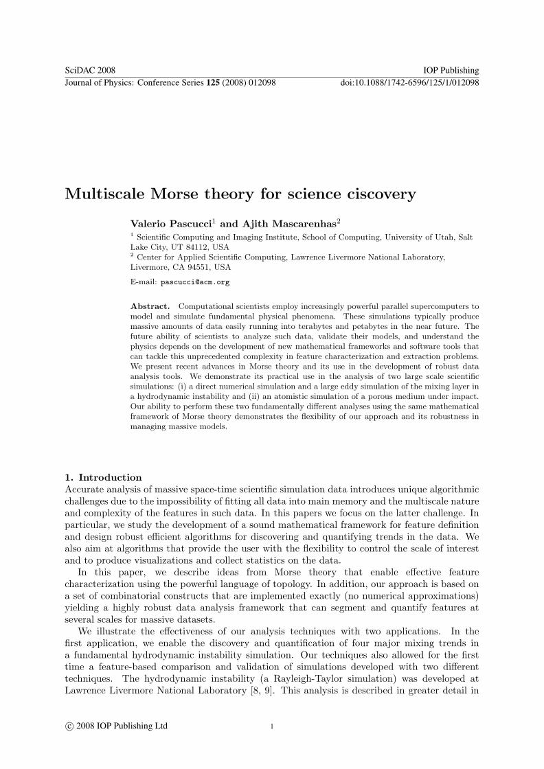
Figure 1. MS-complex construction, simplification and topologically valid approximation: (a)Morse function with critical points shown; (b) stable manifolds; (c) unstable manifolds; (d)MS-complex; (e) MS-complex and manifold after simplification. Maxima are solid blue, minimaare solid white, and saddles are mixed.

[15, 17]. In the second application, we enable the detection of core structures in the atomisticsimulation of a porous medium and their tracking in time as a projectile impacts the mediumcausing structural failures. This analysis is described in detail in [12]. For a more detaileddescription of Morse-theory based analysis see [7, 10, 11, 3, 4, 20].

2. Morse theory for robust multi-scale feature analysisTo begin, we present some background from Morse theory [16, 18] and from combinatorial andalgebraic topology [1, 19].

Smooth maps on manifolds. Let f : M! R be a smooth map. A point x "M is a critical pointof f if the gradient of f vanishes at x, and the value f(x) is a critical value. Noncritical pointsand noncritical values are called regular points and regular values, respectively. A critical pointx is nondegenerate if the Hessian (matrix of second-order partial derivatives) at x is nonsingular.The index of a critical point x, denoted by indexx, is the number of negative eigenvalues of theHessian. For d = 3 there are four types of nondegenerate critical points: the minima (index0), the 1-saddles (index 1), the 2-saddles (index 2), and the maxima (index 3). A function f isMorse if all critical points are nondegenerate with distinct values.

Morse-Smale complex. An integral line is a maximal path on M whose tangent vectors agreewith the gradient of f . The stable manifold of a critical point x is the union of x and allintegral lines that end at x. The unstable manifold of x is defined symmetrically as the unionof a critical point x and all integral lines that start at x. One can superimpose the stable andunstable manifolds of all critical points to create the Morse-Smale complex (or MS complex) off [10, 4], see figure 1(a)–(d). The nodes of this complex are the critical points of f , its arcs areintegral lines starting or ending at saddles, and its regions are the nonempty intersections ofstable and unstable 2-manifolds. More details on the definition of the MS-complex on 2-manifoldtriangle meshes and algorithms to compute it are given by Bremer et al. [4].

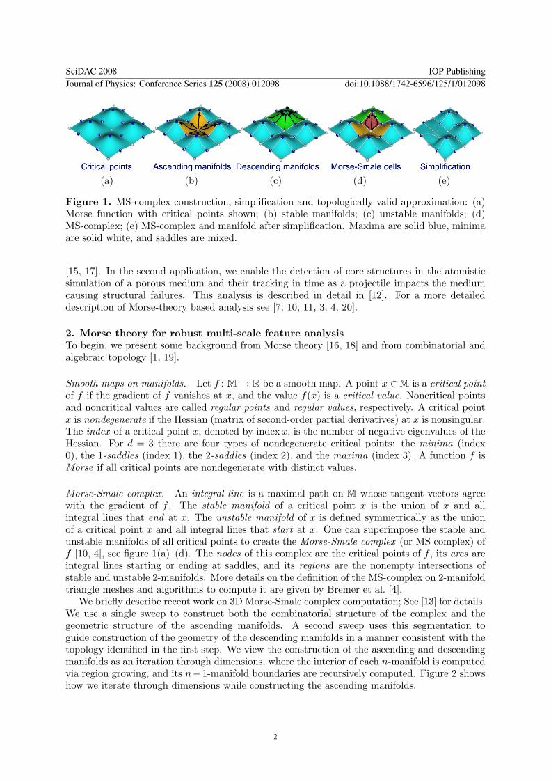
We briefly describe recent work on 3D Morse-Smale complex computation; See [13] for details.We use a single sweep to construct both the combinatorial structure of the complex and thegeometric structure of the ascending manifolds. A second sweep uses this segmentation toguide construction of the geometry of the descending manifolds in a manner consistent with thetopology identified in the first step. We view the construction of the ascending and descendingmanifolds as an iteration through dimensions, where the interior of each n-manifold is computedvia region growing, and its n# 1-manifold boundaries are recursively computed. Figure 2 showshow we iterate through dimensions while constructing the ascending manifolds.

SciDAC 2008 IOP PublishingJournal of Physics: Conference Series 125 (2008) 012098 doi:10.1088/1742-6596/125/1/012098

2

(a) (b) (c) (d) (e)

Figure 2. (a) The algorithm at each iteration identifies interior and boundary vertices of anascending n-manifold. (b) Using minima as seed points, we grow ascending 3-manifolds, findingvertices that are interior (blue) to a single 3-manifold. The grey region depicts the boundarybetween ascending 3-manifolds. (c) We next compute ascending 2-manifolds by first identifyinginterior points. An ascending 2-manifold (green) separates exactly two ascending 3-manifolds.(d) Ascending 1-manifolds (yellow) separate a unique set of ascending 2-manifolds. (e) Finally,the maxima (red) are found as the separating sets between ascending 1-manifolds.

Simplification. It is often useful to simplify an MS-complex to remove noise and to performmulti-scale function analysis. Following [4] we perform cancellations of arc-connected maximum-saddle and minimum-saddle critical point pairs to simplify an MS-complex. Cancellations areranked by their persistence —the absolute di"erence in function value between the canceledcritical point pair. Figure 1(e) and (f) shows an example of a topological simplification and acorresponding approximation of f .

Computation. In practice, one usually deals with piecewise linear (PL)-functions given at thevertices of a triangulation. See [4, 5] for a detailed discussion on how to translate concepts fromthe generic smooth functions discussed above to PL-functions.

Starting from saddles, we compute the arcs of the MS-complex as steepest non-crossingmonotone lines. Because we avoid mesh refinement to handle degeneracies, and instead directlyhandle merged lines and multi-saddles we can use e!cient static data structures to store thetriangulation and can compute MS-complexes of large data sets common in simulation.

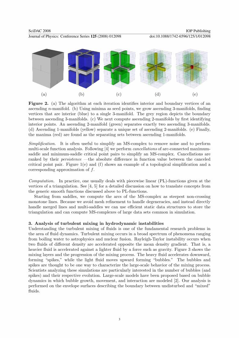
3. Analysis of turbulent mixing in hydrodynamic instabilitiesUnderstanding the turbulent mixing of fluids is one of the fundamental research problems inthe area of fluid dynamics. Turbulent mixing occurs in a broad spectrum of phenomena rangingfrom boiling water to astrophysics and nuclear fusion. Rayleigh-Taylor instability occurs whentwo fluids of di"erent density are accelerated opposite the mean density gradient. That is, aheavier fluid is accelerated against a lighter fluid by a force such as gravity. Figure 3 shows themixing layers and the progression of the mixing process. The heavy fluid accelerates downward,forming “spikes,” while the light fluid moves upward forming “bubbles.” The bubbles andspikes are thought to be one way to characterize the large-scale behavior of the mixing process.Scientists analyzing these simulations are particularly interested in the number of bubbles (andspikes) and their respective evolution. Large-scale models have been proposed based on bubbledynamics in which bubble growth, movement, and interaction are modeled [2]. Our analysis isperformed on the envelope surfaces describing the boundary between undisturbed and “mixed”fluids.

SciDAC 2008 IOP PublishingJournal of Physics: Conference Series 125 (2008) 012098 doi:10.1088/1742-6596/125/1/012098

3

!"#$%&'()*+

(*,!-&'()*+

,.#$*-#-*/0#(

'/.1"&+.*$"2

3*4*0,5".-).6"+&

*0-".'#1"

-&7&8 -&7&988 -&7&:88 -&7&;88

Figure 3. An overview of the 11523 simulation (periodic in x and y) of the Rayleigh-Taylorinstability at start (t = 0), early (t = 200), middle (t = 400), and late (t = 700) time. Thelight fluid has a density of 1.0, the heavy fluid has a density of 3.0. Two envelope surfaces (atdensities 1.02 and 2.98) capture the mixing region. The boundaries of the box show the densityfield in pseudocolor. heavy fluid is red and the light fluid is blue. Totally mixed fluid and themidplanes to study mixing trends.

Segmentation of bubbles. One of the challenges in analyzing the mixing behavior is that thereexists no prevalent mathematical definition for what constitutes a bubble/spike. In general,a bubble can be understood as a three dimensional feature composed of lighter density fluidmoving upwards (in the Z-direction) into a heavier density fluid. We use the topological conceptsintroduced in Section 2 to define bubbles, spikes and other features of interest. Consider theimages of the segmented mixing envelope surface at di"erent times shown to the left, bottom,and right of the plot in figure 4. During early time steps (figure 4 upper left and middle left) it isnatural to consider the mixing envelope as a time-varying functional surface defined over the XY -plane and associate local maxima with bubbles. This analogy fails at later time steps becausethe surface becomes non-functional. However, we can generalize this approach by treating theenvelope surface as the domain of a function whose value at a point x is the Z-coordinate of x.It is natural to connect the maxima of this function to bubbles and compute the stable manifoldof each maximum as a segmentation of the surface into bubbles. As can be seen in figure 4,this segmentation corresponds very well to the human notion of a bubble. Symmetrically, weuse the unstable manifolds of minima to define spikes. Potentially, other functions could bedefined on the envelope surface that would result in a robust segmentation as well. For example,the Z-velocity at all of the points on the envelope surface could be incorporated to capture thefact that bubbles should be moving upwards into the heavy fluid. Given the complexity of theproblem, it has been determined to use the simplest most intuitive segmentation.

In general, topological-based segmentations are often linked to important features: maximaland minimal Z-velocities on the midplanes correspond to cores of rising and falling sections offluids; density extrema correspond to pockets of unmixed fluids. Topological methods are flexibleand enable analysis of a variety of phenomena using the same methodology. Furthermore, theMS-complex can be computed combinatorially [10, 4] which translates into provably correct andstable algorithms which are crucial when dealing with large and complex data.

Multiscale analysis and persistence selection. The MS-complex, just as any other segmentation,captures noise as well as features. A simplification scheme can be used to remove noise andconstruct a series of approximations at decreasing resolution. Unlike many other techniques,topological segmentations allow a simplification scheme that is optimal in the L!-norm. One canformulate the problem of coarsening a segmentation in the following manner: given a functionf and a segmentation S of the domain of f , what is the minimal change on f such thatS is coarsened? If the segmentation one considers is the MS-complex of f , then it can beshown [4] that canceling a critical point pair with persistence p in f requires an approximationf̂ with ||f # f̂ ||! $ p/2. Therefore, canceling critical points in order of increasing persistencecorresponds to an L!-optimal simplification.

SciDAC 2008 IOP PublishingJournal of Physics: Conference Series 125 (2008) 012098 doi:10.1088/1742-6596/125/1/012098

4

100

1000

10000

100000

10 100 1000

00.93%

02.39%

04.84%

Persistence

Threshold

53.0 353 503 700400

slope -0.65

slope -1.72

slope -0.75

Over-segmented

Under-segmented

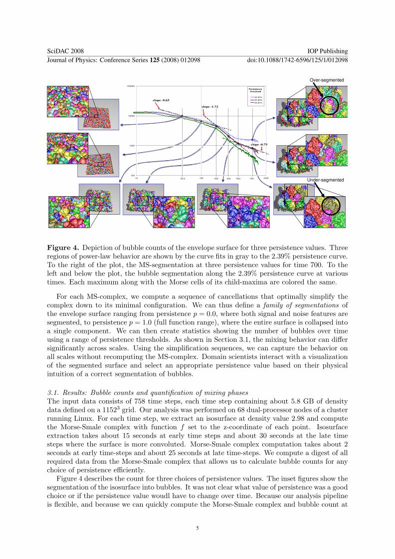
Figure 4. Depiction of bubble counts of the envelope surface for three persistence values. Threeregions of power-law behavior are shown by the curve fits in gray to the 2.39% persistence curve.To the right of the plot, the MS-segmentation at three persistence values for time 700. To theleft and below the plot, the bubble segmentation along the 2.39% persistence curve at varioustimes. Each maximum along with the Morse cells of its child-maxima are colored the same.

For each MS-complex, we compute a sequence of cancellations that optimally simplify thecomplex down to its minimal configuration. We can thus define a family of segmentations ofthe envelope surface ranging from persistence p = 0.0, where both signal and noise features aresegmented, to persistence p = 1.0 (full function range), where the entire surface is collapsed intoa single component. We can then create statistics showing the number of bubbles over timeusing a range of persistence thresholds. As shown in Section 3.1, the mixing behavior can di"ersignificantly across scales. Using the simplification sequences, we can capture the behavior onall scales without recomputing the MS-complex. Domain scientists interact with a visualizationof the segmented surface and select an appropriate persistence value based on their physicalintuition of a correct segmentation of bubbles.

3.1. Results: Bubble counts and quantification of mixing phasesThe input data consists of 758 time steps, each time step containing about 5.8 GB of densitydata defined on a 11523 grid. Our analysis was performed on 68 dual-processor nodes of a clusterrunning Linux. For each time step, we extract an isosurface at density value 2.98 and computethe Morse-Smale complex with function f set to the z-coordinate of each point. Isosurfaceextraction takes about 15 seconds at early time steps and about 30 seconds at the late timesteps where the surface is more convoluted. Morse-Smale complex computation takes about 2seconds at early time-steps and about 25 seconds at late time-steps. We compute a digest of allrequired data from the Morse-Smale complex that allows us to calculate bubble counts for anychoice of persistence e!ciently.

Figure 4 describes the count for three choices of persistence values. The inset figures show thesegmentation of the isosurface into bubbles. It was not clear what value of persistence was a goodchoice or if the persistence value woudl have to change over time. Because our analysis pipelineis flexible, and because we can quickly compute the Morse-Smale complex and bubble count at

SciDAC 2008 IOP PublishingJournal of Physics: Conference Series 125 (2008) 012098 doi:10.1088/1742-6596/125/1/012098

5

VP 2CASC

Mode-Normalized

Bubble Count

Derivative

Bubble Count

-3

-2.5

-2

-1.5

-1

-0.5

0

1

0.01

0.1

1 10 20 303 4 52 6 7 8 9 40

slop

e 1.

536

slop

e 2.

575

slop

e 1.

949

t/! (log scale)

Derivative of

Bubble Count9524 bubbles

linear growth

weak turbulence strong turbulence

mixing transition

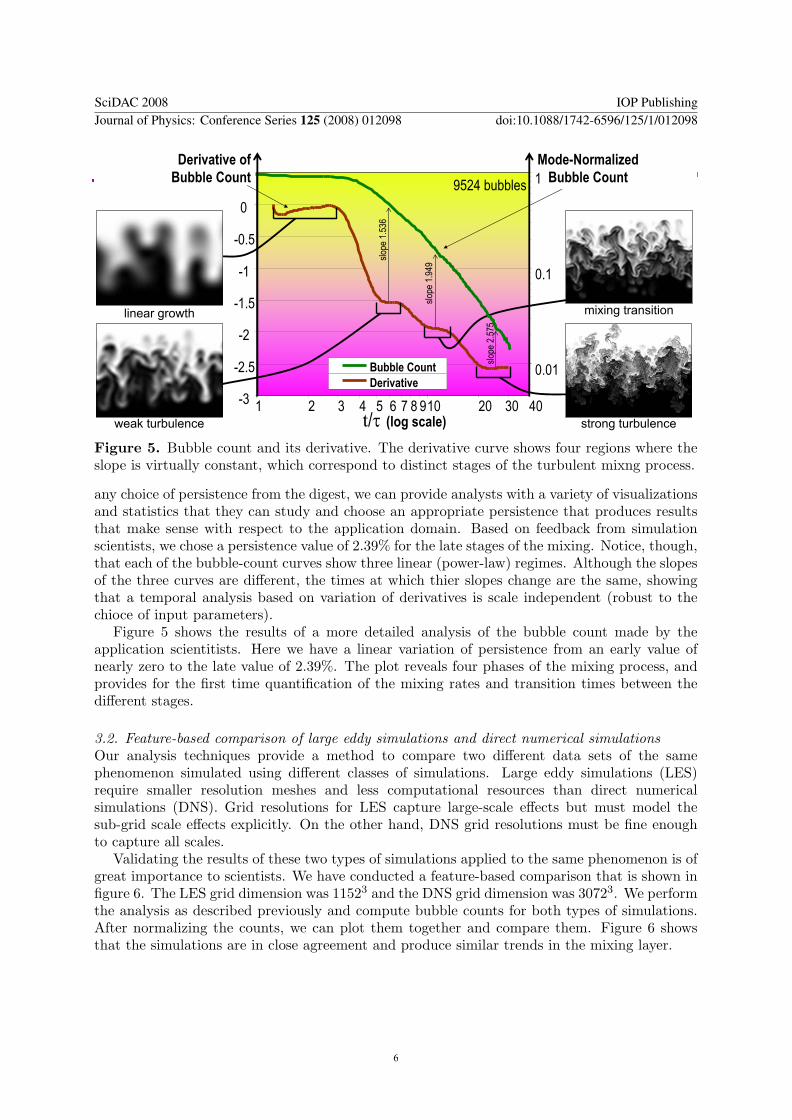
Figure 5. Bubble count and its derivative. The derivative curve shows four regions where theslope is virtually constant, which correspond to distinct stages of the turbulent mixng process.

any choice of persistence from the digest, we can provide analysts with a variety of visualizationsand statistics that they can study and choose an appropriate persistence that produces resultsthat make sense with respect to the application domain. Based on feedback from simulationscientists, we chose a persistence value of 2.39% for the late stages of the mixing. Notice, though,that each of the bubble-count curves show three linear (power-law) regimes. Although the slopesof the three curves are di"erent, the times at which thier slopes change are the same, showingthat a temporal analysis based on variation of derivatives is scale independent (robust to thechioce of input parameters).

Figure 5 shows the results of a more detailed analysis of the bubble count made by theapplication scientitists. Here we have a linear variation of persistence from an early value ofnearly zero to the late value of 2.39%. The plot reveals four phases of the mixing process, andprovides for the first time quantification of the mixing rates and transition times between thedi"erent stages.

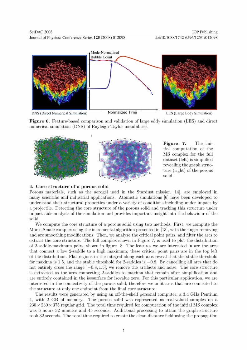
3.2. Feature-based comparison of large eddy simulations and direct numerical simulationsOur analysis techniques provide a method to compare two di"erent data sets of the samephenomenon simulated using di"erent classes of simulations. Large eddy simulations (LES)require smaller resolution meshes and less computational resources than direct numericalsimulations (DNS). Grid resolutions for LES capture large-scale e"ects but must model thesub-grid scale e"ects explicitly. On the other hand, DNS grid resolutions must be fine enoughto capture all scales.

Validating the results of these two types of simulations applied to the same phenomenon is ofgreat importance to scientists. We have conducted a feature-based comparison that is shown infigure 6. The LES grid dimension was 11523 and the DNS grid dimension was 30723. We performthe analysis as described previously and compute bubble counts for both types of simulations.After normalizing the counts, we can plot them together and compare them. Figure 6 showsthat the simulations are in close agreement and produce similar trends in the mixing layer.

SciDAC 2008 IOP PublishingJournal of Physics: Conference Series 125 (2008) 012098 doi:10.1088/1742-6596/125/1/012098

6

VP 1CASC

2 5 10 20 50

0.005

0.01

0.05

0.1

0.5

1

Normalized Time

Mode-Normalized

Bubble Count

DNS (Direct Numerical Simulation)DNS (Direct Numerical Simulation) LES (Large Eddy Simulation)

Figure 6. Feature-based comparison and validation of large eddy simulation (LES) and directnumerical simulation (DNS) of Rayleigh-Taylor instabilities.

Figure 7. The ini-tial computation of theMS complex for the fulldataset (left) is simplifiedrevealing the graph struc-ture (right) of the poroussolid.

4. Core structure of a porous solidPorous materials, such as the aerogel used in the Stardust mission [14], are employed inmany scientific and industrial applications. Atomistic simulations [6] have been developed tounderstand their structural properties under a variety of conditions including under impact bya projectile. Detecting the core structure of the porous solid and tracking this structure underimpact aids analysis of the simulation and provides important insight into the behaviour of thesolid.

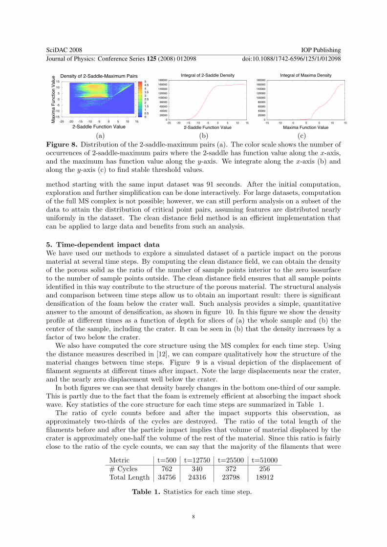
We compute the core structure of a porous solid using two methods. First, we compute theMorse-Smale complex using the incremental algorithm presented in [13], with the finger removingand arc smoothing modifications. Then, we analyze the critical point pairs, and filter the arcs toextract the core structure. The full complex shown in Figure 7, is used to plot the distributionof 2-saddle-maximum pairs, shown in figure 8. The features we are interested in are the arcsthat connect a low 2-saddle to a high maximum; these critical point pairs are in the top leftof the distribution. Flat regions in the integral along each axis reveal that the stable thresholdfor maxima is 1.5, and the stable threshold for 2-saddles is #0.8. By cancelling all arcs that donot entirely cross the range [#0.8, 1.5], we remove the artifacts and noise. The core structureis extracted as the arcs connecting 2-saddles to maxima that remain after simplification andare entirely contained in the isosurface for isovalue zero. For this particular application, we areinterested in the connectivity of the porous solid, therefore we omit arcs that are connected tothe structure at only one endpoint from the final core structure.

The results were generated by using an o"-the-shelf personal computer, a 3.4 GHz Pentium4, with 2 GB of memory. The porous solid was represented as real-valued samples on a230% 230% 375 regular grid. The total time required for computation of the initial MS complexwas 6 hours 32 minutes and 45 seconds. Additional processing to attain the graph structuretook 32 seconds. The total time required to create the clean distance field using the propagation

SciDAC 2008 IOP PublishingJournal of Physics: Conference Series 125 (2008) 012098 doi:10.1088/1742-6596/125/1/012098

7

0 0.5 1 1.5 2 2.5 3 3.5 4 4.5 5

Density of 2-Saddle-Maximum Pairs

-25 -20 -15 -10 -5 0 5 10 15

2-Saddle Function Value

-15

-10

-5

0

5

10

15

Maxim

a F

unction V

alu

e

0

20000

40000

60000

80000

100000

120000

140000

160000

180000

-25 -20 -15 -10 -5 0 5 10 15

2-Saddle Function Value

Integral of 2-Saddle Density

0

20000

40000

60000

80000

100000

120000

140000

160000

180000

-15 -10 -5 0 5 10 15

Maxima Function Value

Integral of Maxima Density

(a) (b) (c)Figure 8. Distribution of the 2-saddle-maximum pairs (a). The color scale shows the number ofoccurrences of 2-saddle-maximum pairs where the 2-saddle has function value along the x-axis,and the maximum has function value along the y-axis. We integrate along the x-axis (b) andalong the y-axis (c) to find stable threshold values.

method starting with the same input dataset was 91 seconds. After the initial computation,exploration and further simplification can be done interactively. For large datasets, computationof the full MS complex is not possible; however, we can still perform analysis on a subset of thedata to attain the distribution of critical point pairs, assuming features are distributed nearlyuniformly in the dataset. The clean distance field method is an e!cient implementation thatcan be applied to large data and benefits from such an analysis.

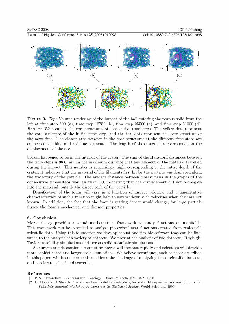
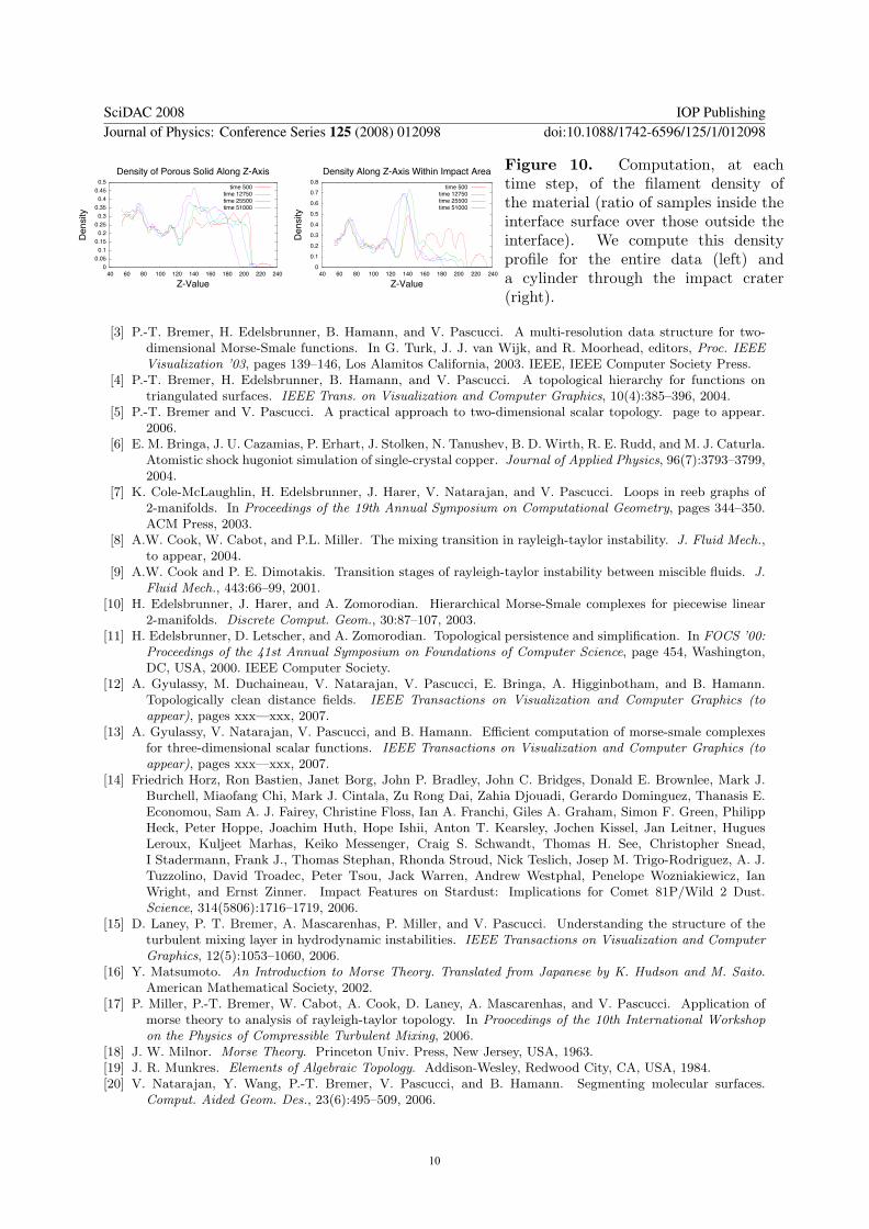
5. Time-dependent impact dataWe have used our methods to explore a simulated dataset of a particle impact on the porousmaterial at several time steps. By computing the clean distance field, we can obtain the densityof the porous solid as the ratio of the number of sample points interior to the zero isosurfaceto the number of sample points outside. The clean distance field ensures that all sample pointsidentified in this way contribute to the structure of the porous material. The structural analysisand comparison between time steps allow us to obtain an important result: there is significantdensification of the foam below the crater wall. Such analysis provides a simple, quantitativeanswer to the amount of densification, as shown in figure 10. In this figure we show the densityprofile at di"erent times as a function of depth for slices of (a) the whole sample and (b) thecenter of the sample, including the crater. It can be seen in (b) that the density increases by afactor of two below the crater.

We also have computed the core structure using the MS complex for each time step. Usingthe distance measures described in [12], we can compare qualitatively how the structure of thematerial changes between time steps. Figure 9 is a visual depiction of the displacement offilament segments at di"erent times after impact. Note the large displacements near the crater,and the nearly zero displacement well below the crater.

In both figures we can see that density barely changes in the bottom one-third of our sample.This is partly due to the fact that the foam is extremely e!cient at absorbing the impact shockwave. Key statistics of the core structure for each time steps are summarized in Table 1.

The ratio of cycle counts before and after the impact supports this observation, asapproximately two-thirds of the cycles are destroyed. The ratio of the total length of thefilaments before and after the particle impact implies that volume of material displaced by thecrater is approximately one-half the volume of the rest of the material. Since this ratio is fairlyclose to the ratio of the cycle counts, we can say that the majority of the filaments that were

Metric t=500 t=12750 t=25500 t=51000# Cycles 762 340 372 256Total Length 34756 24316 23798 18912

Table 1. Statistics for each time step.

SciDAC 2008 IOP PublishingJournal of Physics: Conference Series 125 (2008) 012098 doi:10.1088/1742-6596/125/1/012098

8

(a) (b) (c) (d)& ' & ' & '

Figure 9. Top: Volume rendering of the impact of the ball entering the porous solid from theleft at time step 500 (a), time step 12750 (b), time step 25500 (c), and time step 51000 (d).Bottom: We compare the core structures of consecutive time steps. The yellow dots representthe core structure of the initial time step, and the teal dots represent the core structure ofthe next time. The closest arcs between in the core structures at the di"erent time steps areconnected via blue and red line segments. The length of these segments corresponds to thedisplacement of the arc.

broken happened to be in the interior of the crater. The sum of the Hausdor" distances betweenthe time steps is 98.6, giving the maximum distance that any element of the material travelledduring the impact. This number is surprisingly high, corresponding to the entire depth of thecrater; it indicates that the material of the filaments first hit by the particle was displaced alongthe trajectory of the particle. The average distance between closest pairs in the graphs of theconsecutive timemsteps was less than 5.0, indicating that the displacement did not propagateinto the material, outside the direct path of the particle.

Densification of the foam will vary as a function of impact velocity, and a quantitativecharacterization of such a function might help to narrow down such velocities when they are notknown. In addition, the fact that the foam is getting denser would change, for large particlefluxes, the foam’s mechanical and thermal properties.

6. ConclusionMorse theory provides a sound mathematical framework to study functions on manifolds.This framework can be extended to analyze piecewise linear functions created from real-worldscientific data. Using this foundation we develop robust and flexible software that can be fine-tuned to the analysis of a variety of datasets. We present the analysis of two datasets: Rayleigh-Taylor instability simulations and porous solid atomistic simulations.

As current trends continue, computing power will increase rapidly and scientists will developmore sophisticated and larger scale simulations. We believe techniques, such as those describedin this paper, will become crucial to address the challenge of analyzing these scientific datasets,and accelerate scientific discoveries.

References[1] P. S. Alexandrov. Combinatorial Topology. Dover, Mineola, NY, USA, 1998.[2] U. Alon and D. Shvarts. Two-phase flow model for rayleigh-taylor and richtmeyer-meshkov mixing. In Proc.

Fifth International Workshop on Compressible Turbulent Mixing. World Scientific, 1996.

SciDAC 2008 IOP PublishingJournal of Physics: Conference Series 125 (2008) 012098 doi:10.1088/1742-6596/125/1/012098

9

0

0.05

0.1

0.15

0.2

0.25

0.3

0.35

0.4

0.45

0.5

40 60 80 100 120 140 160 180 200 220 240

De

nsity

Z-Value

Density of Porous Solid Along Z-Axis

time 500time 12750time 25500time 51000

0

0.1

0.2

0.3

0.4

0.5

0.6

0.7

0.8

40 60 80 100 120 140 160 180 200 220 240

De

nsity

Z-Value

Density Along Z-Axis Within Impact Area

time 500time 12750time 25500time 51000

Figure 10. Computation, at eachtime step, of the filament density ofthe material (ratio of samples inside theinterface surface over those outside theinterface). We compute this densityprofile for the entire data (left) anda cylinder through the impact crater(right).

[3] P.-T. Bremer, H. Edelsbrunner, B. Hamann, and V. Pascucci. A multi-resolution data structure for two-dimensional Morse-Smale functions. In G. Turk, J. J. van Wijk, and R. Moorhead, editors, Proc. IEEEVisualization ’03, pages 139–146, Los Alamitos California, 2003. IEEE, IEEE Computer Society Press.

[4] P.-T. Bremer, H. Edelsbrunner, B. Hamann, and V. Pascucci. A topological hierarchy for functions ontriangulated surfaces. IEEE Trans. on Visualization and Computer Graphics, 10(4):385–396, 2004.

[5] P.-T. Bremer and V. Pascucci. A practical approach to two-dimensional scalar topology. page to appear.2006.

[6] E. M. Bringa, J. U. Cazamias, P. Erhart, J. Stolken, N. Tanushev, B. D. Wirth, R. E. Rudd, and M. J. Caturla.Atomistic shock hugoniot simulation of single-crystal copper. Journal of Applied Physics, 96(7):3793–3799,2004.

[7] K. Cole-McLaughlin, H. Edelsbrunner, J. Harer, V. Natarajan, and V. Pascucci. Loops in reeb graphs of2-manifolds. In Proceedings of the 19th Annual Symposium on Computational Geometry, pages 344–350.ACM Press, 2003.

[8] A.W. Cook, W. Cabot, and P.L. Miller. The mixing transition in rayleigh-taylor instability. J. Fluid Mech.,to appear, 2004.

[9] A.W. Cook and P. E. Dimotakis. Transition stages of rayleigh-taylor instability between miscible fluids. J.Fluid Mech., 443:66–99, 2001.

[10] H. Edelsbrunner, J. Harer, and A. Zomorodian. Hierarchical Morse-Smale complexes for piecewise linear2-manifolds. Discrete Comput. Geom., 30:87–107, 2003.

[11] H. Edelsbrunner, D. Letscher, and A. Zomorodian. Topological persistence and simplification. In FOCS ’00:Proceedings of the 41st Annual Symposium on Foundations of Computer Science, page 454, Washington,DC, USA, 2000. IEEE Computer Society.

[12] A. Gyulassy, M. Duchaineau, V. Natarajan, V. Pascucci, E. Bringa, A. Higginbotham, and B. Hamann.Topologically clean distance fields. IEEE Transactions on Visualization and Computer Graphics (toappear), pages xxx—xxx, 2007.

[13] A. Gyulassy, V. Natarajan, V. Pascucci, and B. Hamann. E"cient computation of morse-smale complexesfor three-dimensional scalar functions. IEEE Transactions on Visualization and Computer Graphics (toappear), pages xxx—xxx, 2007.

[14] Friedrich Horz, Ron Bastien, Janet Borg, John P. Bradley, John C. Bridges, Donald E. Brownlee, Mark J.Burchell, Miaofang Chi, Mark J. Cintala, Zu Rong Dai, Zahia Djouadi, Gerardo Dominguez, Thanasis E.Economou, Sam A. J. Fairey, Christine Floss, Ian A. Franchi, Giles A. Graham, Simon F. Green, PhilippHeck, Peter Hoppe, Joachim Huth, Hope Ishii, Anton T. Kearsley, Jochen Kissel, Jan Leitner, HuguesLeroux, Kuljeet Marhas, Keiko Messenger, Craig S. Schwandt, Thomas H. See, Christopher Snead,I Stadermann, Frank J., Thomas Stephan, Rhonda Stroud, Nick Teslich, Josep M. Trigo-Rodriguez, A. J.Tuzzolino, David Troadec, Peter Tsou, Jack Warren, Andrew Westphal, Penelope Wozniakiewicz, IanWright, and Ernst Zinner. Impact Features on Stardust: Implications for Comet 81P/Wild 2 Dust.Science, 314(5806):1716–1719, 2006.

[15] D. Laney, P. T. Bremer, A. Mascarenhas, P. Miller, and V. Pascucci. Understanding the structure of theturbulent mixing layer in hydrodynamic instabilities. IEEE Transactions on Visualization and ComputerGraphics, 12(5):1053–1060, 2006.

[16] Y. Matsumoto. An Introduction to Morse Theory. Translated from Japanese by K. Hudson and M. Saito.American Mathematical Society, 2002.

[17] P. Miller, P.-T. Bremer, W. Cabot, A. Cook, D. Laney, A. Mascarenhas, and V. Pascucci. Application ofmorse theory to analysis of rayleigh-taylor topology. In Proocedings of the 10th International Workshopon the Physics of Compressible Turbulent Mixing, 2006.

[18] J. W. Milnor. Morse Theory. Princeton Univ. Press, New Jersey, USA, 1963.[19] J. R. Munkres. Elements of Algebraic Topology. Addison-Wesley, Redwood City, CA, USA, 1984.[20] V. Natarajan, Y. Wang, P.-T. Bremer, V. Pascucci, and B. Hamann. Segmenting molecular surfaces.

Comput. Aided Geom. Des., 23(6):495–509, 2006.

SciDAC 2008 IOP PublishingJournal of Physics: Conference Series 125 (2008) 012098 doi:10.1088/1742-6596/125/1/012098

10