Multiscale Methods for Porous Media Flow - SINTEF · Outline 1 Introduction to Reservoir Simulation Flow in Porous Media Upscaling 2 Multiscale Methods From Upscaling to Multiscale

Multiscale Methods for Porous Media Flow

Knut–Andreas LieVegard Kippe, Stein Krogstad, Jørg E. Aarnes

SINTEF ICT, Dept. Applied Mathematics

NSCM-18, November 28-29, 2005

Applied Mathematics NSCM-18 1/36

Outline

1 Introduction to Reservoir SimulationFlow in Porous MediaUpscaling

2 Multiscale MethodsFrom Upscaling to Multiscale MethodsMultiscale Mixed Finite Elements

3 Numerical ExamplesMultiscale Methods versus UpscalingComputational ComplexityStrongly Heterogeneous StructuresFlexibility wrt Grids

4 Concluding Remarks


Two-Phase Flow in Porous Media

Pressure equation:

−∇(K(x)λ(S)∇p) = q, v = −K(x)λ(S)∇p,

Fluid transport:

φ∂tS +∇ · (vf(S)) = ε∇(D(S,x)∇S

)Applied Mathematics NSCM-18 3/36

Flow in Porous Media, cont’d

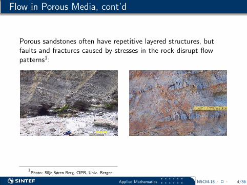
Porous sandstones often have repetitive layered structures, butfaults and fractures caused by stresses in the rock disrupt flowpatterns1:

1Photo: Silje Søren Berg, CIPR, Univ. Bergen


Scales in Porous Media Flow

The scales that impact fluid flow in oil reservoirs range from

the micrometer scale of pores and pore channels

via dm–m scale of well bores and laminae sediments

to sedimentary structures that stretch across entire reservoirs.


Geological ModelsThe knowledge database in the oil company

Geomodels consist of geometry androck parameters (permeability K andporosity φ):

K spans many length scales andhas multiscale structure

maxK/minK ∼ 103–1010

Details on all scales impact flow

Gap between simulation models and geomodels:

High-resolution geomodels may have 107 − 109 cells

Conventional simulators are capable of about 105 − 106 cells

Traditional solution: upscaling of parameters


Geological ModelsThe knowledge database in the oil company

Geomodels consist of geometry androck parameters (permeability K andporosity φ):

K spans many length scales andhas multiscale structure

maxK/minK ∼ 103–1010

Details on all scales impact flow

Gap between simulation models and geomodels:

High-resolution geomodels may have 107 − 109 cells

Conventional simulators are capable of about 105 − 106 cells

Traditional solution: upscaling of parameters


Upscaling Geomodels

Upscaling a geomodel to acoarser simulation grid:

Combine cells to derivecoarse grid

Derive new efficient cellproperties

Fewer cells ⇒ fastersimulation/less storage

However:

Robust upscaling can bedifficult and work-intensive

⇑


Upscaling the Pressure Equation

Assume that u satisfies theelliptic PDE:

−∇(a(x)∇u

)= f.

Upscaling amounts to finding anew field a∗(x) on a coarser gridsuch that

−∇(a∗(x)∇u∗

)= f ,

u∗ ∼ u, q∗ ∼ q .10 20 30 40 50 60

20

40

60

80

100

120

140

160

180

200

220

2 4 6 8 10

2

4

6

8

10

12

14

16

18

20

22

Here the overbar denotes averaged quantities on a coarse grid.


Upscaling the Pressure Equation, cont’d

How do we represent fine-scale heterogeneities on a coarse scale?

Arithmetic, geometric, harmonic, or power averaging(1|V |

∫V a(x)

p dx)1/p

Equivalent permeabilities ( a∗xx = −QxLx/∆Px )

V’

p=1 p=0

u=0

u=0

V

p=1

p=0

u=0 u=0V

V’

Lx

Ly


State-of-the-art in Industry10th SPE Comparative Solution Project

Producer A

Producer B

Producer C

Producer D

Injector

Tarbert

UpperNess

Geomodel: 60× 220× 85 ≈ 1, 1 million grid cells

Simulation: 2000 days of production


10th SPE Comparative Solution ProjectUpscaling results reported by industry

0 200 400 600 800 1000 1200 1400 1600 1800 20000

0.1

0.2

0.3

0.4

0.5

0.6

0.7

0.8

0.9

1

Time (days)

Wat

ercu

t

Fine GridTotalFinaElfGeoquestStreamsimRoxarChevron

0 200 400 600 800 1000 1200 1400 1600 1800 20000

0.1

0.2

0.3

0.4

0.5

0.6

0.7

0.8

0.9

1

Time (days)W

ater

cut

Fine GridLandmarkPhillipsCoats 10x20x10


Developing an Alternative to Upscaling

Observation:

Variations on small scale can have large impact on large-scaleflow patterns

We therefore seek a methodology which:

gives a detailed image of the flow pattern on the fine scale,without having to solve the full fine-scale system

is robust and flexible with respect to the coarse grid

is robust and flexible with respect to the fine grid and thefine-grid solver

is accurate and conservative

is fast and easy to parallelise


From Upscaling to Multiscale Methods

Standard methodUpscaled model:

⇓

⇑

Building blocks:

Two-scale methodGeomodel:

⇓

⇑

Building blocks:

⇓

⇑




⇓

⇑

Building blocks:


⇓

⇑

Building blocks:

⇓

⇑




⇓ ⇑Building blocks:


⇓

⇑

Building blocks:

⇓

⇑






⇓

⇑

Building blocks:

⇓

⇑






⇓

⇑

Building blocks:

⇓

⇑






⇓

⇑

Building blocks:

⇓

⇑






⇓

⇑

Building blocks:

⇓ ⇑







⇓ ⇑


From Upscaling to Multiscale Methods, cont’d

1 Global upscaling methods (Nielsen, Holden, Tveito)

global boundary conditions, minimization of error functional

2 Local-global upscaling methods (Durlofsky et al.)

global boundary conditions + iterative improvement

3 Nested gridding (Gautier, Blunt & Christie)

Upscaling + local reconstruction of fine-scale velocities

4 Multiscale finite elements

basis functions with subscale resolutionfinite elements (Hou & Wu) – pressuremixed elements (Chen & Hou; Aarnes et al.) — velocityfinite volumes (Jenny et al.) — pressure

5 Variatonal multiscale methods (Hughes et al.; Arbogast;Larson & Malqvist; Juanes)

direct decomposition of the solution, V = Vc ⊕ Vf


Multiscale Mixed Finite ElementsFormulation

Mixed formulation:

Find (v, p) ∈ H1,div0 × L2 such that∫

(λK)−1u · v dx−∫p∇ · u dx = 0, ∀u ∈ H1,div

0 ,∫`∇ · v dx =

∫q` dx, ∀` ∈ L2.

Multiscale discretisation:

Seek solutions in low-dimensional subspaces

Ums ⊂ H1,div0 and V ∈ L2,

where local fine-scale properties are incorporated into the basisfunctions.


Multiscale Mixed Finite ElementsGrids and Basis Functions

We assume we are given a fine grid with permeability and porosityattached to each fine-grid block.

We construct a coarse grid, and choose the discretisation spaces Vand Ums such that:

For each coarse block Ti, there is a basis function φi ∈ V .

For each coarse edge Γij , there is a basis function ψij ∈ Ums.










Ti







TiTj





Multiscale Mixed Finite ElementsBasis for the Velocity Field

For each coarse edge Γij , define a basisfunction

ψij : Ti ∪ Tj → R2

with unit flux through Γij and no flowacross ∂(Ti ∪ Tj).

Homogeneous medium Heterogeneous medium

We use ψij = −λK∇φij with

∇ · ψij =

{wi(x), for x ∈ Ti,

−wj(x), for x ∈ Tj ,

with boundary conditions ψij · n = 0 on ∂(Ti ∪ Tj).


Multiscale Mixed Finite ElementsBasis for Velocity Field, cont’d

Homogeneous coefficients and rectangular support domain:basis function = lowest order Raviart-Thomas basis

MsMFEM = extension to cases with subscale variation incoefficients and non-rectangular support domain

Homogeneous medium Heterogeneous medium


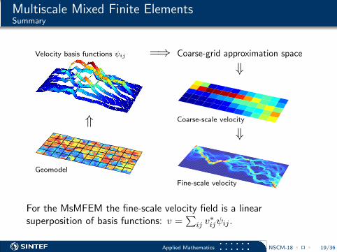
Multiscale Mixed Finite ElementsSummary

Velocity basis functions ψij

⇑

Geomodel

=⇒ Coarse-grid approximation space

⇓

Coarse-scale velocity

⇓

Fine-scale velocity

For the MsMFEM the fine-scale velocity field is a linearsuperposition of basis functions: v =

∑ij v

∗ijψij .


Properties of the MsMFEM

Multiscale:Incorporates small-scale effects into coarse-scale solution

Conservative:Mass conservative on coarse grid and on the subgrid scale

Scalable:Well suited for parallel implementation since basis functions areprocessed independently

Flexible:No restrictions on subgrids and subgrid numerical method. Fewrestrictions on the shape of the coarse blocks

Fast:The method is fast when avoiding regeneration of (most of) thebasis functions at every time step


Examples: AccuracySPE10 Revisited (5× 11× 17 Coarse Grid)

0 500 1000 1500 20000

0.2

0.4

0.6

0.8

1

Time (days)

Wat

ercu

tProducer A

0 500 1000 1500 20000

0.2

0.4

0.6

0.8

1

Time (days)

Wat

ercu

t

Producer B

0 500 1000 1500 20000

0.2

0.4

0.6

0.8

1

Time (days)

Wat

ercu

t

Producer C

0 500 1000 1500 20000

0.2

0.4

0.6

0.8

1

Time (days)

Wat

ercu

t

Producer D

ReferenceMsMFEM Nested Gridding




Nested gridding: upscaling + downscaling


Multiscale vs. UpscalingSPE10, Layer 85 (15× 55 Grid)

0 100 200 300 400 500 6000

50

100

150

200

250

300

350

0.1

0.2

0.3

0.4

0.5

0.6

0.7

0.8

0.9

0 100 200 300 400 500 6000

50

100

150

200

250

300

350

0.1

0.2

0.3

0.4

0.5

0.6

0.7

0.8

0.9

reference (240× 880) MsMFEM MsFVM

0 100 200 300 400 500 6000

50

100

150

200

250

300

350

0.1

0.2

0.3

0.4

0.5

0.6

0.7

0.8

0.9

0 100 200 300 400 500 6000

50

100

150

200

250

300

350

0.1

0.2

0.3

0.4

0.5

0.6

0.7

0.8

0.9

0 100 200 300 400 500 6000

50

100

150

200

250

300

350

0.1

0.2

0.3

0.4

0.5

0.6

0.7

0.8

0.9

ALGU-NG pressure method harmonic-arithmetic


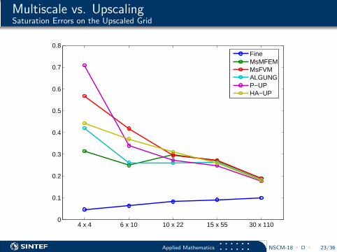
Multiscale vs. UpscalingSaturation Errors on the Upscaled Grid

4 x 4 6 x 10 10 x 22 15 x 55 30 x 1100

0.1

0.2

0.3

0.4

0.5

0.6

0.7

0.8FineMsMFEMMsFVMALGUNGP−UPHA−UP


Multiscale vs. Upscaling/Downscaling

0 100 200 300 400 500 6000

50

100

150

200

250

300

350

0.1

0.2

0.3

0.4

0.5

0.6

0.7

0.8

0.9

reference (240× 880) MsMFEM

0 100 200 300 400 500 6000

50

100

150

200

250

300

350

0.1

0.2

0.3

0.4

0.5

0.6

0.7

0.8

0.9

0 100 200 300 400 500 6000

50

100

150

200

250

300

350

0.1

0.2

0.3

0.4

0.5

0.6

0.7

0.8

0.9

MsFVM ALGU-NG


Multiscale vs. UpscalingSaturation Errors on the Fine Grid

4 x 4 6 x 10 10 x 22 15 x 55 30 x 1100

0.1

0.2

0.3

0.4

0.5

0.6

0.7FineMsMFEMMsFVMALGUNGP−UPHA−UP


RobustnessSPE10, Layer 85 (60× 220 Grid)


Computational ComplexityOrder of Magnitude Argument

Example: 3D (128x128x128), α = 1.2 and m = 3

8^3 16^3 32^3 64^30

0.5

1

1.5

2

2.5

3

3.5

4

4.5 x 108

Fine scale sol. ↓

MsFVMMsMFEMLGNGALGNG


Computational ComplexityComments

Direct solution more efficient, so why bother with multiscale?

Full simulation: O(102) steps.

Basis functions need not be recomputed

2^3 4^3 8^3 16^3 32^3 64^3 128^30

1

2

3

4

5

6

7

8

9

10 x 109

LocalGlobal

Also:

Possible to solve very large problems

Easy parallelization


Strongly Heterogeneous Structures

Logarithm of kx

0 20 40 60 80 100 1200

20

40

60

80

100

120

−7

−6

−5

−4

−3

−2

−1

0

1

2

3

kred = 104

kyellow = 1kblue = 10−8

Coarse grid = 8× 8.

0 20 40 60 80 100 1200

20

40

60

80

100

120

0.1

0.2

0.3

0.4

0.5

0.6

0.7

0.8

0.9

Reference

0 20 40 60 80 100 1200

20

40

60

80

100

120

0.1

0.2

0.3

0.4

0.5

0.6

0.7

0.8

0.9

MsMFEM


Problem: Traversing Barriers

Problems occur when a basis function forces flow through a barrier:

Potential problem No problem

Problem-cases can be detected automatically through the indicator

υij = ψij · (λK)−1ψij .

If υij(x) > C for some x ∈ Ti, then split Ti, and generate basisfunctions for the new faces.


Problem: Traversing Barriers

Problems occur when a basis function forces flow through a barrier:

Potential problem No problem

Problem-cases can be detected automatically through the indicator

υij = ψij · (λK)−1ψij .

If υij(x) > C for some x ∈ Ti, then split Ti, and generate basisfunctions for the new faces.


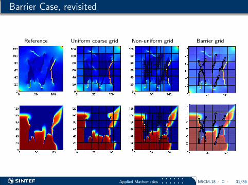
Barrier Case, revisited

Reference Uniform coarse grid Non-uniform grid Barrier grid


Flexibility wrt. Grids


Flexibility wrt. GridsAround Flow Barriers


Flexibility wrt. GridsAround Wells


Flexibility wrt. GridsFracture Networks

2

2Courtesy of M. Karimi-Fard, Stanford


Concluding Remarks

Upscaling is and will be an important part of the reservoirmodelling workflow

Multiscale methods may replace upscaling/downscaling forsimulation purposes, because they:

give better resolution

are more flexible

may be faster

However, a lot of (exciting) research needs to be done..


Multiscale Methods for Porous Media Flow - SINTEF · Outline 1 Introduction to Reservoir Simulation Flow in Porous Media Upscaling 2 Multiscale Methods From Upscaling to Multiscale

Documents