Multiscale Damage Modeling for Composite Materials - SCoReC

1

Multiscale Damage Modeling for Composite Materials: Theory and Computational Framework

Jacob Fish and Qing YuDepartments of Civil, Mechanical and Aeronautical Engineering

Rensselaer Polytechnic InstituteTroy, NY 12180

Abstract

A nonlocal multiscale continuum damage model is developed for brittle composite materials.A triple-scale asymptotic analysis is generalized to account for the damage phenomena occur-ring at micro-, meso- and macro- scales. A closed form expressions relating microscopic,mesoscopic and overall strains and damage is derived. The damage evolution is stated on thesmallest scale of interest and nonlocal weighted phase average fields over micro- and meso-phases are introduced to alleviate the spurious mesh dependence. Numerical simulation con-ducted on a composite beam made of Blackglas/Nextel 2D weave is compared with the testdata.

1.0 Introduction

Damage phenomena in composite materials are very complex due to significant heterogene-

ities and interactions between microconstituents. Typically, damage can be either discrete or

continuous and described on at least three different scales: discrete for atomistic voids and lat-

tice defects; and continuous for micromechanical and macromechanical scales, which

describe either distributed microvoids and microcracks or discrete cracks whose size is com-

parable to the structural component. Here, attention is restricted to continuum scales only. On

the micromechanical scale, the Representative Volume Element (RVE) is introduced to model

the initiation and growth of microscopic damage and their effects on the material behavior.

The RVE is defined to be small enough to distinguish microscopic heterogeneities, but suffi-

ciently large to represent the overall behavior of the heterogeneous medium. Most research in

this area is focused on the two-scale micro-macro problems with homogeneous microconstitu-

ents. For certain composite materials systems, such as woven composites [43], the two-scale

model might be insufficient due to strong heterogeneities in one of the microphases. The ques-

tion arises as to how to account for damage effects in these heterogeneous phases. Most com-

monly, macroscopic-like point of view [12], [30], [32], [34], [39] is adopted by idealizing the

2

heterogeneous phases as anisotropic homogeneous media. Anisotropic continuum damage

theory is then employed to model damage evolution in each phase. As an alternative, which is

explored here, is to define smaller scale RVE(s) for the heterogeneous phases and then to carry

out multiple scale damage analysis with various RVEs at different length scales.

The objective of this paper is to extend the two-scale (macro-micro) nonlocal damage theory

developed in [22] to three scales in attempt to account for evolution of damage in heteroge-

neous microphases. Throughout the manuscript we term the larger scale RVE(s) as mesos-

copic while RVE(s) comprising heterogeneous meso-phases as microscopic. In Section 2, the

three-scale (macro-, meso- and micro-) damage theory within the framework of the mathemat-

ical homogenization theory is developed. The triple-scale asymptotic expansions of damage

and displacements lead to closed form expressions relating local (microscopic and mesos-

copic) fields to overall (macroscopic) strains and damage. In Section 3, the nonlocal phase

fields for multi-phase composites are defined as weighted averages over each phase in the

mesoscopic and microscopic characteristic volumes with piecewise constant weight functions.

A more general case of weight functions is discussed in [22]. In Section 4, a simplified variant

of the nonlocal damage model for the two-phase composite materials is developed. The com-

putational framework including stress update procedure and consistent tangent stiffness are

presented in Section 5. In Section 6, we first study the axial loading capacity of the Blackglas/

Nextel 2-D woven composite [11][43]. Numerical results obtained by the present three-scale

formulation are compared with those obtained by the two-scale model [22]. We then consider

a 4-point bending test conducted on the composite beam made of Blackglas/Nextel 2-D

woven composite and compare the simulation results with the experiments data provided by

[11]. Discussion and future research directions conclude the manuscript.

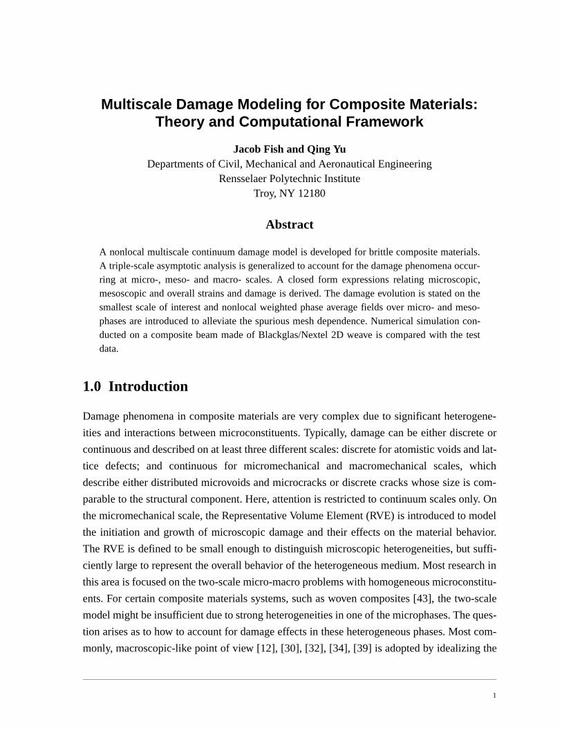
2.0 Mathematical Homogenization for Damaged Composites

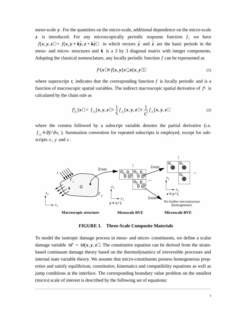
As shown in Figure 1 , the composite material is represented by two locally periodic RVEs on

the meso-scale (Y-periodic) and the micro-scale (Z-periodic), denoted by and , respec-

tively. Let be the macroscopic coordinate vector in the macro domain ; be the

mesoscopic position vector in and be the microscopic position vector in .

Here, denotes a very small positive number; and are regarded as the

stretched local coordinate vectors. When a solid is subjected to some load and boundary con-

ditions, the resulting deformation, stresses, and internal variables may vary from point to point

within the RVE(s) due to a high level of heterogeneity. We assume that all quantities on the

meso-scale have two explicit dependences: one on the macro-scale and the other on the

Θy Θz

x Ω y x ς⁄≡Θy z y ς⁄≡ Θz

ς y x ς⁄≡ z y ς⁄≡

x

3

meso-scale . For the quantities on the micro-scale, additional dependence on the micro-scale

is introduced. For any microscopically periodic response function , we have

in which vectors and are the basic periods in the

meso- and micro- structures and is a 3 by 3 diagonal matrix with integer components.

Adopting the classical nomenclature, any locally periodic function can be represented as

(1)

where superscript indicates that the corresponding function is locally periodic and is a

function of macroscopic spatial variables. The indirect macroscopic spatial derivative of is

calculated by the chain rule as

(2)

where the comma followed by a subscript variable denotes the partial derivative (i.e.

). Summation convention for repeated subscripts is employed, except for sub-

scripts , and .

FIGURE 1. Three-Scale Composite Materials

To model the isotropic damage process in meso- and micro- constituents, we define a scalar

damage variable . The constitutive equation can be derived from the strain-

based continuum damage theory based on the thermodynamics of irreversible processes and

internal state variable theory. We assume that micro-constituents possess homogeneous prop-

erties and satisfy equilibrium, constitutive, kinematics and compatibility equations as well as

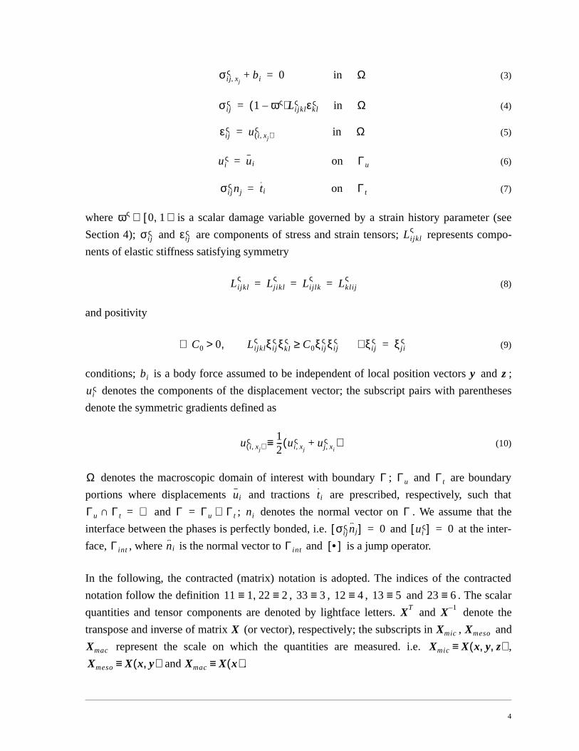
jump conditions at the interface. The corresponding boundary value problem on the smallest

(micro) scale of interest is described by the following set of equations:

y

z f

f x y z, ,( ) f x y ky+ z kz+, ,( )= y z

k

f

fς x( ) f x y x( ) z x y,( ), ,( )≡

ς f

fς

f,xi

ς x( ) f,xix y z, ,( ) 1

ς--- f,yi

x y z, ,( ) 1

ς2---- f,zi

x y z, ,( )+ +=

f,xi∂f ∂xi⁄≡

x y z

z1

z2

Ω

tZoom

ΘyΓt

Γu

y x ς⁄≡

Macroscopic structure

b

...

...

Θz

ΘyΘy

Θz

Θz...

...Zoom

ZoomNo further microstructure

(homogenous)x1

x2

y1

y2

z y ς⁄≡

Mesoscale RVE Microscale RVE

ως ω x y z, ,( )=

4

(3)

(4)

(5)

(6)

(7)

where is a scalar damage variable governed by a strain history parameter (see

Section 4); and are components of stress and strain tensors; represents compo-

nents of elastic stiffness satisfying symmetry

(8)

and positivity

(9)

conditions; is a body force assumed to be independent of local position vectors and ;

denotes the components of the displacement vector; the subscript pairs with parentheses

denote the symmetric gradients defined as

(10)

denotes the macroscopic domain of interest with boundary ; and are boundary

portions where displacements and tractions are prescribed, respectively, such that

and ; denotes the normal vector on . We assume that the

interface between the phases is perfectly bonded, i.e. and at the inter-

face, , where is the normal vector to and is a jump operator.

In the following, the contracted (matrix) notation is adopted. The indices of the contracted

notation follow the definition , , , and . The scalar

quantities and tensor components are denoted by lightface letters. and denote the

transpose and inverse of matrix (or vector), respectively; the subscripts in , and

represent the scale on which the quantities are measured. i.e. ,

and .

σi j x j,ς bi+ 0 in Ω=

σ i jς 1 ως–( )Lijkl

ς εklς in Ω=

εi jς u i x, j( )

ς in Ω=

uiς ui on Γu=

σi jς nj ti on Γt=

ως 0 1),[∈σi j

ς εi jς Lijkl

ς

Lijklς Ljikl

ς Lijlkς Lklij

ς= = =

C0 0 Lijklς ξi j

ς ξklς C0ξi j

ς ξi jς ξi j

ς∀≥,>∃ ξj iς=

bi y z

uiς

u i x, j( )ς 1

2--- ui x, j

ς uj x, i

ς+( )≡

Ω Γ Γu Γt

ui ti

Γu Γt∩ ∅= Γ Γu Γt∪= ni Γσi j

ς nj[ ] 0= uiς[ ] 0=

Γint ni Γint •[ ]

11 1 22 2≡,≡ 33 3≡ 12 4≡ 13 5≡ 23 6≡XT X 1–

X Xmic Xmeso

Xmac Xmic X x y z, ,( )≡Xmeso X x y,( )≡ Xmac X x( )≡

5

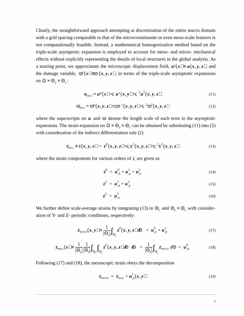
Clearly, the straightforward approach attempting at discretization of the entire macro domain

with a grid spacing comparable to that of the microconstituents or even meso-scale features is

not computationally feasible. Instead, a mathematical homogenization method based on the

triple-scale asymptotic expansion is employed to account for meso- and micro- mechanical

effects without explicitly representing the details of local structures in the global analysis. As

a starting point, we approximate the microscopic displacement field, , and

the damage variable, , in terms of the triple-scale asymptotic expansions

on :

(11)

(12)

where the superscripts on and denote the length scale of each term in the asymptotic

expansions. The strain expansion on can be obtained by substituting (11) into (5)

with consideration of the indirect differentiation rule (2)

(13)

where the strain components for various orders of are given as

(14)

(15)

(16)

We further define scale-average strains by integrating (13) in and with consider-

ation of Y- and Z- periodic conditions, respectively:

(17)

(18)

Following (17) and (18), the mesoscopic strain obeys the decomposition

(19)

uς x( ) u x y z, ,( )≡ως x( ) ω x y z, ,( )≡

Ω Θy Θz××

umic u0 x( ) ςu1 x y,( ) ς2u2 x y z, ,( )+ +≈

ωmic ω0 x y z, ,( ) ςω1 x y z, ,( ) ς2ω2 x y z, ,( )+ +≈

u ωΩ Θy Θz××

εmic ε x y z, ,( )≡ ε0 x y z, ,( ) ςςε1 x y z, ,( ) ςς2ε2 x y z, ,( )+ +=

ς

ε0 u,x0 u,y

1 u,z2+ +=

ε1 u,x1 u,y

2 +=

ε2 u,x2 =

Θz Θy Θz×

εmeso x y,( ) 1Θz--------- ε0 x y z, ,( ) Θd

Θz

∫≡ u,x0 u,y

1+=

εmac x( ) 1Θy---------

1Θz--------- ε0 x y z, ,( ) Θ Θdd

Θz

∫Θy

∫≡ 1Θy--------- εmeso Θd

Θy

∫ u,x0= =

εmeso εmac u,y1 x y,( )+=

6

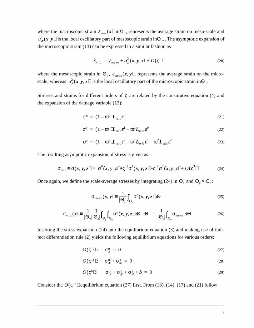
where the macroscopic strain in , represents the average strain on meso-scale and

is the local oscillatory part of mesoscopic strain in . The asymptotic expansion of

the microscopic strain (13) can be expressed in a similar fashion as

(20)

where the mesoscopic strain in , , represents the average strain on the micro-

scale, whereas is the local oscillatory part of the microscopic strain in .

Stresses and strains for different orders of are related by the constitutive equation (4) and

the expansion of the damage variable (12):

(21)

(22)

(23)

The resulting asymptotic expansion of stress is given as

(24)

Once again, we define the scale-average stresses by integrating (24) in and :

(25)

(26)

Inserting the stress expansion (24) into the equilibrium equation (3) and making use of indi-

rect differentiation rule (2) yields the following equilibrium equations for various orders:

(27)

(28)

(29)

Consider the equilibrium equation (27) first. From (13), (14), (17) and (21) follow

εmac x( ) Ωu,y

1 x y,( ) Θy

εmic εmeso u,z2 x y z, ,( ) O ς( )+ +=

Θy εmeso x y,( )u,z

2 x y z, ,( ) Θz

ς

σ0 1 ω0–( )Lmicε0=

σ1 1 ω0–( )Lmicε1 ω1Lmicε0–=

σ2 1 ω0–( )Lmicε2 ω1Lmicε

1– ω2Lmicε0–=

σmic σ x y z, ,( )≡ σ0 x y z, ,( ) ς1σ1 x y z, ,( ) ς2σ2 x y z, ,( ) O ς3( )+ + +=

Θz Θy Θz×

σmeso x y,( ) 1Θz--------- σ0 x y z, ,( ) Θd

Θz

∫≡

σmac x( ) 1Θy---------

1Θz--------- σ0 x y z, ,( ) Θ Θdd

Θz

∫Θy

∫≡ 1Θy--------- σmeso Θd

Θy

∫=

O ς 2–( ): σ,z0 0=

O ς 1–( ): σ,y0 σ,z

1+ 0=

O ς0( ): σ,x0 σ,y

1 σ,z2+ + b+ 0=

O ς 2–( )

7

(30)

(31)

where is a history-dependent microscopic stiffness.

To solve for (30) we introduce the following decomposition:

(32)

where the third order tensor is symmetric with respect to indices and

[19][22] and Z-periodic in . We assume that is mesoscopic damage-induced

strain driven by mesoscopic strain . More specifically, we can state that if

, then and . However, vice versa is not true, i.e., if or

, the mesoscopic strain may not be necessarily zero.

Based on the decomposition given in (32), equilibrium equation takes the following

form:

(33)

where is identity matrix and

(34)

is a micro-scale polarization function. The integrals of the polarization function in vanish

due to periodicity conditions. Since equation (33) should be valid for arbitrary mesoscopic

fields, we may first consider the case of (and ) but , which

yields:

(35)

Equation (35) together with the Z-periodic boundary conditions comprise a linear boundary

value problem for in . The weak form of (35) is solved for three right hand side vectors

in 2-D and six in 3-D (see for example [21][26]). In absence of damage, the strain asymptotic

expansions (13) and (20) can be expressed in terms of the mesoscopic strain as

(36)

Lmicεmic ,z Lmic εmeso u,z2+( ) ,z 0 in Θz= =

Lmic 1 ω0 x y z, ,( )– Lmic=

Lmic

u2 x y z, ,( ) H z( ) εmeso x y,( ) dmeso x y,( )+ =

H z( ) Hikl z( )≡ k l

Θz dmeso x y,( )εmeso x y,( )

εmeso 0= dmeso 0= ω0 0= dmeso 0=

ω0 0= εmeso

O ς 2–( )

Lmic I Gz+( )εmeso Gzdmeso+ ,z 0 in Θz=

I

Gz z( ) H,z z( ) H i ,zj( )kl z( )≡=

Θz

dmeso 0= ω0 0= εmeso 0≠

Lmic I Gz+( ) ,z 0=

H Θz

εmeso

εmic Az εmeso O ς( )+=

8

where is elastic strain concentration function in defined as

(37)

After solving (35) for , we proceed to finding from (33). Premultiplying it by and

integrating it by parts in with consideration of Z-periodic boundary conditions yields

(38)

and the expression for the mesoscopic damage induced strain becomes

(39)

Let and be the two sets of

continuous functions, then the damage variable is assumed to have the fol-

lowing decomposition

(40)

where is the macroscopic damage variable; is a damage distribution function

on the meso-scale RVE; represents the damage distribution function in the micro-

scale RVE corresponding to phase in the meso-scale RVE. Rewriting (39) in terms of

and yields

(41)

where

(42)

(43)

(44)

(45)

Az Θz

Az I Gz+=

H dmeso H

Θz

GzTLmic Azεmeso Gzdmeso+( ) Θd

Θz

∫ 0=

dmeso GzTLmicGz Θd

Θz

∫

–1–

= GzTLmicAz Θd

Θz

∫

εmeso

f f α( ) y( ) α 1 2 …, ,=; ≡ g g αβ( ) z( ) α β, 1 2 …, ,=; ≡C 1– ω0 x y z, ,( )

ω0 x y z, ,( ) ω x( )f α( ) y( ) g αβ( ) z( )β∑

α∑=

ω x( ) f α( ) y( )g αβ( ) z( )

β αAmic ω0 x y z, ,( )

dmeso Dmesoεmeso=

Dmeso I ω x( )f α( ) y( ) B αβ( )

β∑

α∑–

1–

ω x( )f α( ) y( ) C αβ( )

β∑

α∑

=

B αβ( ) 1Θz--------- Lmeso Lmeso–( )

1–g αβ( ) z( )Gz

TLmicGz ΘdΘz

∫=

C αβ( ) 1Θz--------- Lmeso Lmeso–( )

1–g αβ( ) z( )Gz

TLmicAz ΘdΘz

∫=

Lmeso1

Θz--------- Lmic Θd

Θz

∫=

9

(46)

where is the overall stiffness on ; is the elastic homogenized stiffness

[19][22]; denotes the volume of the micro-scale RVE. Note that the integrals in

and are history-independent and thus can be precomputed. This provides one of the

main motivations for the decomposition given in (40).

Based on (32) and (41), the asymptotic expansion of the strain field (13) can be finally cast as

(47)

where is a local damage strain distribution function in . Note that the asymptotic expan-

sion of the strain field is given as a sum of mechanical fields induced by the mesoscopic strain

via elastic strain concentration function and thermodynamical fields governed by the dam-

age-induced strain through the distribution function .

We now consider the equilibrium equation (28). By integrating (28) over , making

use of the Z-periodicity condition and the definition of the mesoscopic stress in (25), we get

(48)

which represents the mesomechanical equilibrium equation in . Based on the asymptotic

expansion of the strain field in (13) and (19), the constitutive equation in (21) and the decom-

position (47) we can rewrite (48) as

(49)

(50)

where is a history-dependent mesoscopic stiffness matrix.

To solve for the mesomechanical equilibrium equation, we first note that (49) is similar to its

microscopic counterpart in (30). Thus, a similar procedure can be employed by introducing

the decomposition:

(51)

Lmeso1

Θz--------- LmicAz Θd

Θz

∫ 1Θz--------- Az

TLmicAz ΘdΘz

∫= =

Lmeso Θz Lmeso

Θz B αβ( )

C αβ( )

εmic Az GzDmeso+( )εmeso O ς( ) +=

Gz Θz

Az

dmeso Dmesoεmeso= Gz

O ς 1–( ) Θz

σmeso( ),y1

Θz--------- σ0 x y z, ,( ) Θd

Θz

∫

,y

0 in Θy= =

Θy

Lmesoεmeso ,y Lmeso εmac u,y1+( ) ,y 0 in Θy= =

Lmeso1

Θz--------- Lmic Az GzDmeso+( ) Θd

Θz

∫=

Lmeso

u1 x y,( ) H y( ) εmac x( ) dmac x( )+ =

10

where is a Y-periodic third order tensor on the meso-scale, symmetric with

respect to indices and ; is the macroscopic damage-induced strain driven by the

macroscopic strain . Based on this decomposition, (49) becomes:

(52)

where

(53)

is a polarization function on the meso-scale whose integral in vanishes due to Y-periodic-

ity conditions. Once again, since (53) is valid for arbitrary macroscopic fields, we first con-

sider the case of damage-free, i.e. and but , which yields:

(54)

Equation (54) comprise a linear boundary value problem for in the meso-scale domain

subjected to Y-periodic boundary conditions. Based on the decomposition in (51) and in

absence of damage, the mesoscopic strain in (19) can be expressed in terms of the macro-

scopic strain as:

(55)

where is the mesoscopic elastic strain concentration function defined as

(56)

After obtaining , can be obtained from (52) by premultiplying it with and integrat-

ing it by parts in with consideration of Y-periodic boundary conditions, which yields

(57)

(58)

where in (50) is a history-dependent stiffness matrix. Based on the decomposition of

the damage variable in (40), is given as

H y( ) Hikl y( )≡k l dmac x( )εmac x( )

Lmeso I Gy+( )εmac Gydmac+ ,y 0 in Θy=

Gy y( ) H,y y( ) H i ,yj( )kl y( )≡=

Θy

dmac 0= ω0 0= εmac 0≠

Lmeso I Gy+( ) ,y 0=

H Θy

εmac

εmeso Ay εmac=

Ay

Ay I Gy+=

H dmac H

Θy

dmac Dmac= εmac

Dmac GyTLmesoGy Θd

Θy

∫

–1–

GyTLmesoAy Θd

Θy

∫

=

Lmeso

Lmeso

11

(59)

where

(60)

(61)

To this end, the mesoscopic strain (19) and the asymptotic expansion of the microscopic strain

field (13) can be directly linked to the macroscopic strain as

(62)

(63)

where , the counterpart of in , is a local distribution function of the damage-induced

strain in .

Finally, we integrate the equilibrium equation (29) over . The and

terms in the integral vanish due to periodicity and we obtain:

(64)

Substituting the constitutive relation (21), the asymptotic expansion of the strain field (63), the

microscopic and mesoscopic instantaneous stiffnesses in (31) and (50) into (64) yields the

macroscopic equilibrium equation

(65)

where

(66)

is a macroscopic instantaneous secant stiffness.

Lmeso Lmeso ω x( )f α( ) y( ) Lmesoαβ( )

β∑

α∑–

I D meso+( )

Lmeso ω x( )f α( ) y( ) Lmesoαβ( )

β∑

α∑–

Dmeso–

=

Lmesoαβ( ) 1

Θz--------- g αβ( ) z( )Lmic Θd

Θz

∫=

Lmesoαβ( ) 1

Θz--------- g αβ( ) z( )LmicAz Θd

Θz

∫=

εmeso Ay GyDmac+( )εmac =

εmic Az GzDmeso+( ) Ay GyDmac+( )εmac O ς( ) +=

Gy Gz Θz

Θy

O ς0( ) Θy Θz× σ,y1 Θd

Θy

∫σ,z

2 ΘdΘz

∫1

Θy---------

1Θz--------- σ0 x y z, ,( ) Θ Θdd

Θz

∫Θy

∫

,x

b+ 0= in Ω

σmac( ),x b+ 0 and = Lmacεmac( ),x b+ 0=

Lmac1

Θy--------- Lmeso Ay GyDmac+( ) Θd

Θy

∫=

12

3.0 Nonlocal Piecewise Constant Damage Model for Multi-Phase Materials

Accumulation of damage leads to strain softening and loss of ellipticity in quasi-static prob-

lems. The local approach, stating that in absence of thermal effects, stresses at a material point

are completely determined by the deformation and the deformation history at that point, may

result in a physically unacceptable localization of the deformation [4]-[7], [13], [24]. A num-

ber of regularization techniques have been developed to limit strain localization and to allevi-

ate mesh sensitivity associated with strain softening [4]-[10], [13], [14], [15]. One of these

approaches is based on smearing solution variables causing strain softening over the charac-

teristic volume of the material [4][6]. Following [6] and [22], the nonlocal damage variable

is defined as:

(67)

where and are weight functions on micro- and meso-scale, respectively; and

are the characteristic volumes on the micro- and meso- scales with characteristic length

and , respectively. The characteristic length is defined (for example) as a radius of the

largest inscribed sphere in a characteristic volume, which is related to the size of the material

inhomogeneties [6]. and are the radii of the largest inscribed spheres in the Statistically

Homogeneous Volumes (SHV), which is the smallest volume for which the corresponding

local periodicity assumptions are valid. Several guidelines for determining the value of char-

acteristic length have been provided in [5] and [24]. The characteristic lengths, and , as

indicated in [6], are usually smaller than the corresponding and in particular for ran-

dom local structures. Following the two-scale nonlocal damage model in [22], we redefine the

Representative Volume Element (RVE) as the maximum between Statistically Homogeneous

Volume and the characteristic volume. Schematically, this can be expressed as

(68)

(69)

where and denote the radii of the largest inscribed spheres in the mesoscopic

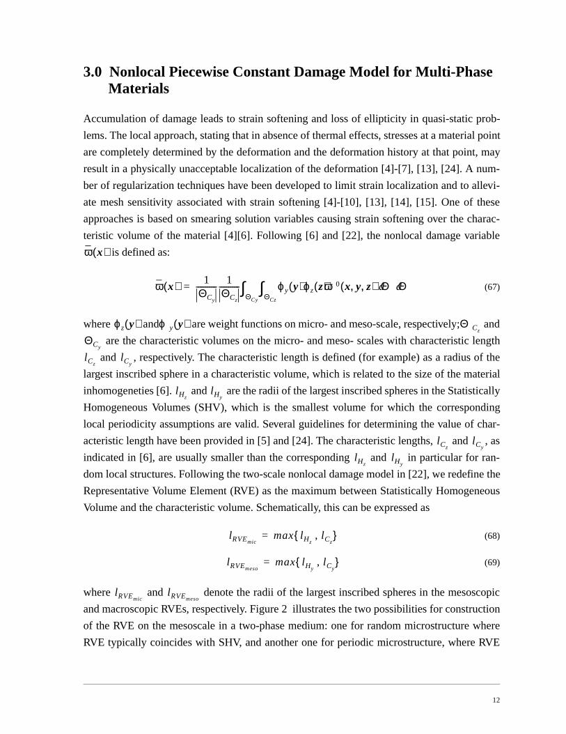
and macroscopic RVEs, respectively. Figure 2 illustrates the two possibilities for construction

of the RVE on the mesoscale in a two-phase medium: one for random microstructure where

RVE typically coincides with SHV, and another one for periodic microstructure, where RVE

ω x( )

ω x( ) 1ΘCy

-----------1

ΘCz

----------- ϕy y( )ΘCz

∫ ϕz z( )ω0 x y z, ,( ) Θ ΘddΘCy

∫=

ϕz y( ) ϕy y( ) ΘCz

ΘCy

lCzlCy

lHzlHy

lCzlCy

lHzlHy

lRVEmicmax lHz

, lCz =

lRVEmesomax lHy

, lCy =

lRVEmiclRVEmeso

13

and SHV are of the same order of magnitude. Figure 2 is also applicable to the definition of

the microscopic RVE.

FIGURE 2. Selection of the Representative Volume Element

In particular, we assume that the microscopic and mesoscopic damage distribution functions,

and in (40), are both piecewise constant; is assumed to be unity

within the domain of the mesoscopic phase which satisfies , and to van-

ish elsewhere, i.e.

(70)

where and ; is a product

of the number of different mesoscopic phases and the number of mesoscopic characteristic

volumes in the mesoscopic RVE ; is unity within the microphase , such that

, but vanish elsewhere, i.e.

(71)

where and ; is the

product of the number of different microphases and the number of microscopic characteristic

volumes in .

Θy

lCy

lHy

Θy

lCy ( lHy

)≈

Characteristic Volumes ΘCy

g αβ( ) z( ) f α( ) y( ) f α( ) y( )Θy

α( ) Θyα( ) ΘCy

Θy⊂ ⊂

f α( ) y( ) 1 if y Θy

α( )∈

0 otherwise

=

Θyα( )

α 1=

kα

∪ Θy= Θyi( ) Θy

j( )∩ ∅ for i j and i j, 1= 2 … kα, , ,≠= kα

Θy g αβ( ) z( ) Θzαβ( )

Θzαβ( ) ΘCz

α( ) Θzα( )⊂ ⊂

g αβ( ) z( ) 1 if z Θz

αβ( )∈

0 otherwise

=

Θzαβ( )

β 1=

kαβ

∪ Θzα( )= Θy

i( ) Θyj( )∩ ∅ for i j and i j, 1= 2 … kαβ, , ,≠= kαβ

Θzα( )

14

We further define the weight function in (67) as

and (72)

where the constants and are determined by the orthogonality conditions

(73)

(74)

and are the Kronecker deltas. Substituting (40) and (70)-(74) into (67) shows that

coincides with the nonlocal phase average damage variable:

(75)

The average strains in each microphase, termed as microscopic phase average strain, are

obtained by integrating (63) over

(76)

where represents the domain of phase in

and (77)

and (78)

(79)

and following (43)-(46) and (71) yields

(80)

(81)

ϕy y( ) µyα( )f α( ) y( )= ϕz z( ) µz

αβ( )g αβ( ) z( )=

µyα( ) µz

αβ( )

µyα( )

ΘCy

----------- f α( ) y( )f α( ) y( ) Θ δαα , α α,=dΘCy

∫ 1 2 … kα, , ,=

µzαβ( )

ΘCz

α( )------------- g αβ( ) z( )g αβ( ) z( ) Θ δββ , β β,=d

ΘCzα( )∫ 1 2 … kαβ, , ,=

δαα δββ

ω αβ( )

ω x( )µy

α( )

ΘCy

-----------µz

αβ( )

ΘCz

α( )------------- ω x( ) f α( ) y( )g αβ( ) z( ) 2

ΘCzα( )∫ Θ Θdd

ΘCy

∫ ω αβ( ) x( )≡=

Θzαβ( )

εmesoαβ( ) 1

Θzαβ( )

--------------- εmic ΘdΘz

αβ( )∫ Azαβ( ) Gz

αβ( )Dmesoα( )+( ) Ay

α( ) Gyα( )Dmac+( )εmac = =

Θzαβ( ) β Θz

α( )

Gyα( ) Gy y Θy

α( )∈( )≡ Ayα( ) I G+ y

α( )=

Gzαβ( ) 1

Θzαβ( )

--------------- Gz z( ) ΘdΘz

αβ( )∫= Az

αβ( ) I G+ zαβ( )

=

Dmesoα( ) Dmeso x y Θy

α( )∈,( )≡ I ω αβ( )B αβ( )

α∑–

1–

ω αβ( )C αβ( )

β∑

=

B αβ( ) 1

Θzα( )

------------- Lmesoα( )

Lmesoα( )

–( )1–

GzTLmicGz Θd

Θzαβ( )

∫=

C αβ( ) 1

Θzα( )

------------- Lmesoα( )

Lmesoα( )

–( )1–

GzTLmicAz Θd

Θzαβ( )

∫=

15

(82)

(83)

We denote the volume fractions for phase in by such that

. It can be readily seen that

(84)

Similarly, the phase average strain in the mesoscopic RVE can be obtained by integrating

(62) over , which yields

(85)

where the mesoscopic phase average strain concentration function is defined as

and (86)

Also, we have the relation

(87)

where is the volume fraction of phase in satisfying

To construct the nonlocal constitutive relation between phase averages, we define the local

average stress in as:

(88)

By combining (88) with microscopic constitutive equation (21), the asymptotic expansion of

strain in (13) and (47) and the piecewise constant damage variable defined in (40), (70) and

(71), we get

(89)

Lmesoα( ) 1

Θzα( )------------- Lmic Θd

Θzα( )∫=

Lmesoα( ) 1

Θzα( )------------- LmicAz Θd

Θzα( )∫ 1

Θzα( )------------- Az

TLmicAz ΘdΘz

α( )∫= =

β Θzα( ) v αβ( ) Θz

αβ( ) Θzα( )⁄≡

vβ∑αβ( )

1=

εmesoα( ) εmeso x y Θy

α( )∈,( )≡ v αβ( )εmesoαβ( )

β∑=

Θy

Θyα( )

εmacα( ) 1

Θyα( )

------------- εmeso ΘdΘy

α( )∫ Ayα( ) Gy

α( )Dmac+( )εmac = =

Ayα( )

Gyα( ) 1

Θyα( )

------------- Gy y( ) ΘdΘy

α( )∫= Ay

α( ) I G+ yα( )

=

εmac v α( )εmacα( )

α∑=

v α( ) Θyα( ) Θy⁄≡ α Θy vα∑

α( )1=

Θzα( )

σmesoαβ( ) 1

Θzαβ( )--------------- σ0 x y z, ,( ) Θd

Θzαβ( )∫≡

σmesoαβ( ) 1 ω αβ( )–( )Lmseo

αβ( ) εmesoαβ( )=

16

where . Here, we assume that each phase in the micro-

scale RVE is homogeneous, i.e. is assumed to be independent of the position vector

within each phase .

The phase average stress in the mesoscopic RVE is defined in a similar fashion to (88) as:

(90)

With the definition of in (25), the microscopic constitutive equation (21), equations (31)

and (50), the definition in (90) can be restated as

(91)

where the macroscopic phase average instantaneous secant stiffness in is given as

(92)

and

and (93)

which follows from (26) and (91). The mesoscopic instantaneous stiffness can be

obtained from (59) in conjunction with the definition of the piecewise constant damage so that

(94)

where the phase average stiffness and the homogenized stiffness are obtained

from (60) and (61):

and (95)

The constitutive equations (89) and (91) have a nonlocal character in the sense that they relate

between phase averages in the microscopic and mesoscopic RVEs, respectively. The response

characteristics between the phases are not smeared as the damage evolution law and thermo-

Lmesoαβ( ) Lmic x y Θy

α( )∈ z Θzαβ( )∈, ,( )≡

Lmesoαβ( ) z

Θzαβ( )

Θy

σmacα( ) 1

Θyα( )------------- σmeso Θd

Θyα( )∫≡

σmeso

σmacα( ) Lmac

α( ) εmac =

Lmacα( ) Θy

α( )

Lmacα( ) 1

Θyα( )------------- Lmeso

α( ) Ay GyDmac+( ) ΘdΘy

α( )∫=

σmac vα∑

α( )σmac

α( )= Lmac vα∑

α( )Lmac

α( )=

Lmesoα( )

Lmesoα( ) Lmeso x y Θy

α( )∈,( )

≡

Lmeso v αβ( )ω αβ( )Lmesoαβ( )

β∑–

I D mesoα( )+( ) Lmeso v αβ( )ω αβ( )Lmeso

αβ( )

β∑–

Dmesoα( )–=

Lmesoαβ( ) Lmeso

αβ( )

Lmesoαβ( ) 1

Θzαβ( )--------------- Lmic Θd

Θzαβ( )∫= Lmeso

αβ( ) 1

Θzαβ( )--------------- LmicAz Θd

Θzαβ( )∫=

17

mechanical properties of phases might be significantly different, in particular when damage

occurs in a single phase. In the next section we focus on the multiscale damage modeling in

woven composites.

4.0 Damage Evolution for Two-Phase Composites

As a special case depicted in Figure 1, we consider a three-scale composite whose mesoscopic

structure is composed of reinforcement phase and matrix phase such that

and the volume fractions satisfy . We assume that the

matrix phase in the mesoscopic RVE is homogeneous and isotropic, i.e. the stiffness

of matrix is independent of any position vectors such that

(96)

Since the matrix phase in is homogeneous, there are no microscopic structures for ,

and therefore and in . From (79)-(83), follows that

(97)

For the reinforcement phase , we assume that it consists of a two-phase composite (rein-

forcement and matrix ) characterized by the microscopic RVE , such that

and .

For simplicity, we further assume that damage occurs in the matrix only. The expression of the

damage variable (40), (70) and (71) can be further simplified for this special case as

(98)

Accordingly, the mesoscopic instantaneous stiffness for and in (94) becomes

(99)

(100)

where

α F=( ) α M=( )Θy Θy

F( ) ΘyM( )∪= v F( ) v M( )+ 1=

ΘyM( ) Θy

LmesoM( ) Lmeso

M( )Lmac

M( )≡ ≡ constant=

Θy ΘyM( )

Gz 0≡ Az I≡ ΘyM( )

DmesoM( ) 0≡

ΘyF( )

β f= β m= ΘzF( )

ΘzF( ) Θz

Ff( ) ΘzFm( )∪= v Ff( ) v Fm( )+ 1=

ω0 x y z, ,( )

ω M( ) x( ) y ΘyM( ) ∈

ω Fm( ) x( ) y ΘyF( ) and z Θz

Fm( )∈∈

0 otherwise

=

ΘyF( ) Θy

M( )

LmesoF( ) Lmeso

F( )v Fm( )ω Fm( )Lmeso

Fm( )– I D meso

F( )+( ) LmesoF( )

v Fm( )ω Fm( )LmesoFm( )

– DmesoF( )–=

LmesoM( ) 1 ω M( )–( )Lmac

M( )=

18

(101)

The macroscopic phase average instantaneous stiffness ( ) given in (92) takes

the following form:

(102)

(103)

The expression of can be further modified by substituting (99) and (100)

(104)

The damage variable is assumed to be a monotonically increasing func-

tion of nonlocal phase deformation history parameter (see, for example, [12], [22], [24],

[27], [28] and [38]) which characterizes the maximum deformation experienced throughout

the loading history. In general, the evolution of phase damage at time can be expressed as

(105)

where ; the operator denotes the positive part, i.e.

; the phase deformation history parameter is determined by the

evolution of the nonlocal phase damage equivalent strain, denoted by

(106)

where represents the threshold value of the damage equivalent strain prior to the initia-

tion of phase damage. Based on the strain-based damage theory [38] we defined the damage

equivalent strain as

(107)

DmesoF( ) I ω Fm( )B Fm( )–( ) 1– ω Fm( )C Fm( )=

Lmacα( ) α F M,=

LmacF( ) 1

ΘyF( )------------- Lmeso

F( ) Ay GyDmac+( ) ΘdΘy

F( )∫=

LmacM( ) Lmeso

M( ) AyM( ) Gy

M( )Dmac+( )=

Dmac

Dmac GyTLmeso

F( ) Gy ΘdΘy

F( )∫ GyTLmeso

M( ) Gy ΘdΘy

M( )∫+

–1–

GyTLmeso

F( ) Ay ΘdΘy

F( )∫ GyTLmeso

M( ) Ay ΘdΘy

M( )∫+

=

ω η( ) η M Fm,=( )κ η( )

t

ω η( ) x t,( ) f < κ η( ) x t,( ) ϑiniη( ) >+–( ) and

f κ η( ) x t,( )( )∂κ η( )∂

------------------------------- 0≥=

η M Fm,= < >+

< >• + sup 0 , •= κ η( )

ϑη( )

κ η( ) x t,( ) max ϑ η( ) x τ,( ) τ t≤( ) , ϑini

η( ) =

ϑini

η( )

ϑη( )

ϑ η( ) 12--- F η( )εmac

η( )( )

TLmac

M( ) F η( )εmacη( )

( ) η M Fm,=,=

19

where represents the principal nonlocal phase strain vector, i.e.

and is the mapping of in the corresponding principal

strain directions; denotes the weighting matrix aimed at accounting for different damage

accumulation in tension and compression

(108)

(109)

where and are constants selected to represent the contributions of each component of

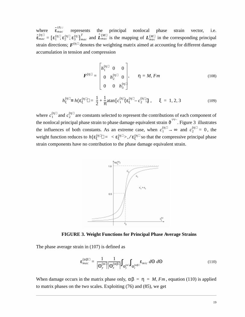
the nonlocal principal phase strain to phase damage equivalent strain . Figure 3 illustrates

the influences of both constants. As an extreme case, when and , the

weight function reduces to so that the compressive principal phase

strain components have no contribution to the phase damage equivalent strain.

FIGURE 3. Weight Functions for Principal Phase Average Strains

The phase average strain in (107) is defined as

(110)

When damage occurs in the matrix phase only, , equation (110) is applied

to matrix phases on the two scales. Exploiting (76) and (85), we get

εmac

η( )

εmacη( )

ε1η( ) ε2

η( ) ε3η( ), ,[ ]= mac

TLmac

M( )Lmac

M( )

F η( )

F η( )

h1η( ) 0 0

0 h2η( ) 0

0 0 h3η( )

η M Fm,=,=

hξη( ) h εξ

η( )( )≡ 12---

1π--- c1

η( ) εξη( ) c2

η( )–( )[ ]atan , ξ+ 1 2 3, ,= =

c1η( ) c2

η( )

ϑη( )

c1η( ) ∞→ c2

η( ) 0=

h εξη( )( ) < εξ

η( ) >+ εξη( )⁄=

εmacαβ( ) 1

Θyα( )-------------

1

Θzαβ( )--------------- εmic

Θzαβ( )∫ Θ Θdd

Θyα( )∫=

αβ η M Fm,= =

20

(111)

(112)

The arctangent form evolution law [22]

(113)

is adopted, in which are material parameters; denotes the critical value of thestrain history parameter beyond which the damage will develop very quickly.

Based on the definition of the phase damage equivalent strain in (107), the damage evo-lution conditions can be expressed as

(114)

(115)

where denotes the rate of damage.

5.0 Computational issues

In this section, we describe the computational aspects of the nonlocal piecewise constant dam-

age model for the two-phase material developed in Section 4.0. Due to the nonlinear character

of the problem an incremental analysis is employed. Prior to the nonlinear analysis elastic

strain concentration factors, and , are computed in the mesoscopic and micro-

scopic RVEs, respectively, using the finite element method. Subsequently, the phase average

elastic strain concentration factor and the damage distribution factor are precom-

puted using (86), (78) and subsequently and are evaluated.

εmacFm( ) 1

ΘyF( )

------------- AzFm( ) Gz

Fm( )DmesoF( )+( ) Ay GyDmac+( ) Θ εmacd

ΘyF( )∫=

εmacM( ) Ay

M( ) GyM( )Dmac+( )εmac =

Φ η( )

a η( ) < ϑ η( ) ϑini

η( ) >+–

ϑ0

η( )----------------------------------------

b η( )–

b η( )( )atan+atan

π2--- b η( )( )atan+

---------------------------------------------------------------------------------------------------------------------- ω η( )–≡ 0 η, M Fm,= =

a η( ) b η( ), ϑ0

η( )

ϑ η( )

if ϑ η( ) κ η( )– 0, κ· η( )0 damage process: ⇒ ω· η( )

0>>=

if ϑ η( ) κ η( )– 0<or

if ϑ η( ) κ η( )– 0, κ·η( )

0== elastic process: ⇒ ω· η( )

0=

ω·η( )

Gy y( ) Gz z( )

AyM( )

GyM( )

AzFM( )

GzFm( )

21

5.1 Stress update (integration) procedure

Given: displacement vector ; overall strain ; strain history parameters and

; phase damage variables and ; and displacement increment calcu-

lated from the finite element analysis for the global problem. The left subscript denotes the

increment step, i.e., is the variables in the current increment, whereas is a con-

verged variable from the last increment. For simplicity, we will omit the left subscript for the

current increment, i.e., , and use superscript to denote the matrix

phases in both mesoscopic and microscopic RVEs.

Find: overall strain ; nonlocal strain history parameters and ; nonlocal phase

damage variables and ; overall stress and nonlocal phase stresses and

.

The stress update procedure consists of the following steps:

step i.) Calculate the macroscopic strain increment, , and update macroscopic

strains through .

step ii.) Compute the damage equivalent strain defined by (111) and (112) in terms of

and .

step iii.) Check the damage evolution conditions (114) and (115). Note that is defined by

(106) and is integrated as . The procedure for strain and damage

variable updates is given as:

IF: elastic process, and , THEN

set and with

ELSE: damage process,

update for and by solving the system of nonlinear equations (113);

set

IF: elastic process in mesoscopic matrix phase, i.e. , THEN

set and ;

update for and by solving (113) with only;

set

ENDIF

IF: elastic process in microscopic matrix phase, i.e. , THEN

ut mac εt mac κ M( )t

κ Fm( )t ω M( )

t ω Fm( )t ∆umac

t t∆+ t

t t∆+≡ η M Fm,=( )

εmac κ M( ) κ Fm( )

ω M( ) ω Fm( ) σmac σmacF( )

σmacM( )

∆εεmac ∆= u,x

εmac εt mac ∆εmac+=

ϑ η( )

ω η( )t εmac

κ η( )

κ· η( ) κ η( )∆ κ η( ) κ η( )t–=

ϑ M( ) κ M( )t≤ ϑ Fm( ) κ Fm( )

t≤ω η( ) ω η( )

t= κ η( ) κ η( )t= η M Fm,≡

ϑ η( ) ω η( )

κ η( ) ϑ η( )=

ϑ M( ) κ M( )t<

ω M( ) ω M( )t= κ M( ) κ M( )

t=

ϑ Fm( ) ω Fm( ) η Fm=

κ Fm( ) ϑ Fm( )=

ϑ Fm( ) κ Fm( )t<

22

set and ;

update for and by solving (113) with only;

set

ENDIF

ENDIF

Since is determined by the current phase average strains in the meso- and micro-scale

matrix phases, which in turn depend on the current damage variable, it follows that the dam-

age evolution laws in (113) comprise a set of nonlinear equations for . Using the New-

ton’s method we construct an iterative process for the damage variables on both scales:

(116)

The derivatives with respect to and in (116) can be evaluated by differentiating

(113) with provided that the damage processes occur on both

scales, such that

, (117)

, (118)

where and are given as

(119)

The derivatives of the nonlocal damage equivalent strain and with respect to the

damage variables are presented in Appendix.

When damage process occurs only on one scale, either micro- or meso-scale, the set of nonlin-

ear equations (113) reduces to a single nonlinear function and the Newton’s iterative method

gives

ω Fm( ) ω Fm( )t= κ Fm( ) κ Fm( )

t=

ϑ M( ) ω M( ) η M=

κ M( ) ϑ M( )=

ϑ η( )

ω η( )

ω M( )k 1+

ω Fm( )k 1+

ω M( )k

ω Fm( )k

Φ M( )∂ω M( )∂

--------------Φ M( )∂ω Fm( )∂

----------------

Φ Fm( )∂ω M( )∂

----------------Φ Fm( )∂ω Fm( )∂

----------------ω η( )k

1–

Φ M( )

Φ Fm( )ω η( )k

–=

ω M( ) ω Fm( )

κ η( ) ϑη( )

= η M Fm,=( )

Φ M( )∂ω M( )∂

-------------- γ M( ) ϑ M( )∂ω M( )∂

------------- 1–=Φ M( )∂ω Fm( )∂

---------------- γ M( ) ϑ M( )∂ω Fm( )∂

----------------=

Φ Fm( )∂ω M( )∂

---------------- γ Fm( ) ϑ Fm( )∂ω M( )∂

---------------=Φ Fm( )∂ω Fm( )∂

---------------- γ Fm( ) ϑ Fm( )∂ω Fm( )∂

---------------- 1–=

γ M( ) γ Fm( )

γ η( ) a η( )κ0η( ) π 2⁄ b η( )( )atan+ ⁄

κ0η( )( )2 a η( ) ϑ η( ) ϑini

η( )–( ) b η( )κ0

η( )– 2

+------------------------------------------------------------------------------------------------ η M Fm,=,=

ϑM( )

ϑFm( )

23

(120)

where is given in (117) for and in (118) for .

step vi.) Update the nonlocal phase stresses, and , using (91) with macroscopic

instantaneous stiffness and defined in (102) and (103), respectively. The macro-

scopic stress can be finally obtained from (93).

5.2 Consistent tangent stiffness

To this end we focus on the computation of the consistent tangent stiffness matrix on the

macro level. We start by taking material derivative of the incremental form of the constitutive

equation (91)

, (121)

where can be obtained by taking time derivative of (102) and (103), which yields

(122)

(123)

Following (99) and (100), the rate form of the mesoscopic stiffness is given as

, (124)

where

(125)

(126)

and in (125) is obtained by taking time derivative of (101)

(127)

ω η( )k 1+ ω η( )k Φ η( )∂ω η( )∂

-------------

1–

Φ η( )

ω η( )k η, M or Fm=–=

Φ η( )∂ ω η( )∂⁄ η M= η Fm=

σmacF( ) σmac

M( )

LmacF( ) Lmac

M( )

σmac

σ· macF( )

L·

macF( ) εmac Lmac

F( ) ε·mac+= σ· macM( )

L·

macM( ) εmac Lmac

M( ) ε·mac+=

L·

macα( )

L·

macF( ) 1

ΘyF( )------------- L

·mesoF( )

Ay GyDmac+( ) LmesoF( ) GyD

·mac+ Θd

ΘyF( )∫=

L·

macM( )

L·

mesoM( )

AyM( ) Gy

M( )Dmac+( ) LmesoM( ) Gy

M( )D·

mac+=

L·

mesoF( ) Lmeso

F( ) ω· Fm( )= L

·mesoM( ) Lmeso

M( ) ω· M( )=

LmesoF( )

LmesoF( )

LmesoF( )

–( ) v Fm( )ω Fm( ) LmesoFm( )

LmesoFm( )

–( )– DmesoF( )

v Fm( ) LmesoFm( )

LmesoFm( )

LmesoFm( )

–( )DmesoF( )+ –

=

LmesoM( )

LmacM( )–=

DmesoF( )

DmesoF( )

DmesoF( ) Dmeso

F( ) ω· Fm( )≡ I ω Fm( )B Fm( )–( ) 2–C Fm( )ω· Fm( )=

24

From (124)-(127), the time derivative of defined in (104) can be expressed as

(128)

where

(129)

(130)

Substituting (124) and (128) into (122) and (123), the rate form of the macroscopic phase

stiffness becomes

(131)

(132)

where

(133)

(134)

(135)

(136)

To this end, the rate form of the constitutive equation (121) takes the following form

(137)

Dmac

D·

mac DmacM( ) ω· M( ) Dmac

Fm( )ω· Fm( )+=

DmacM( ) Gy

TLmesoF( ) Gy Θd

ΘyF( )∫ Gy

TLmesoM( ) Gy Θd

ΘyM( )∫+

–1–

GyTLmeso

M( ) Gy ΘDmacdΘy

M( )∫ GyTLmeso

M( ) Ay ΘdΘy

M( )∫+

=

DmacFm( )

GyTLmeso

F( ) Gy ΘdΘy

F( )∫ GyTLmeso

M( ) Gy ΘdΘy

M( )∫+

–1–

GyTLmeso

F( ) Gy ΘDmacdΘy

F( )∫ GyTLmeso

F( ) Ay ΘdΘy

F( )∫+

=

L·macF( )

LmacFM( )ω· M( )

LmacFF( )ω· Fm( )

+=

L·macM( )

LmacMM( )ω· M( )

LmacMF( )ω· Fm( )

+=

LmacFM( ) 1

ΘyF( )

------------- LmesoF( ) Gy ΘDmac

M( )d

ΘyF( )∫=

LmacFF( ) 1

ΘyF( )

------------- LmesoF( ) Ay GyDmac+( ) Θd

ΘyF( )∫ Lmeso

F( ) Gy ΘDmacB( )

dΘy

F( )∫+

=

LmacMM( ) Lmeso

M( ) AyM( ) Gy

M( )Dmac+( ) LmesoM( ) Gy

M( )DmacM( )+=

LmacMF( ) Lmeso

M( ) GyM( )Dmac

B( )=

σ· macF( )

LmacFM( )εmacω·

M( ) Lmac

FF( )εmacω·Fm( )

LmacF( ) ε·mac+ +=

25

(138)

In order to obtain and , we make use of damage cumulative law (113) with consid-

eration of damage/elastic processes as described in Section 5.1. In the case of elastic process,

and/or . For damage process, and are obtained by taking

time derivatives of (113). The derivation is detailed in Appendix and the final expressions can

be summarized as

, (139)

Substituting (139) into (137) and (138), we get the following relations between the rate of the

overall strain and the nonlocal phase average stresses in the matrix phases:

, (140)

where

(141)

(142)

The overall consistent tangent stiffness is constructed by substituting (140) into the rate form

of the overall stress-strain relation (93)

(143)

(144)

Finally, we remark that the integrals in the mesoscopic RVE, (129) and (130), have to be eval-

uated at each Gaussian point in the global finite element mesh and for every load increment.

This may lead to enormous computational complexity, especially when the finer mesh is used

for mesoscopic RVE. A close look at the above formulations reveals that the source of the

computational complexity stems from the history-dependent form of . To remedy the

situation, we make use of Taylor expansion in (101) with respect to so that the history-

dependent variable can be moved out of the integrals.

6.0 Numerical Examples

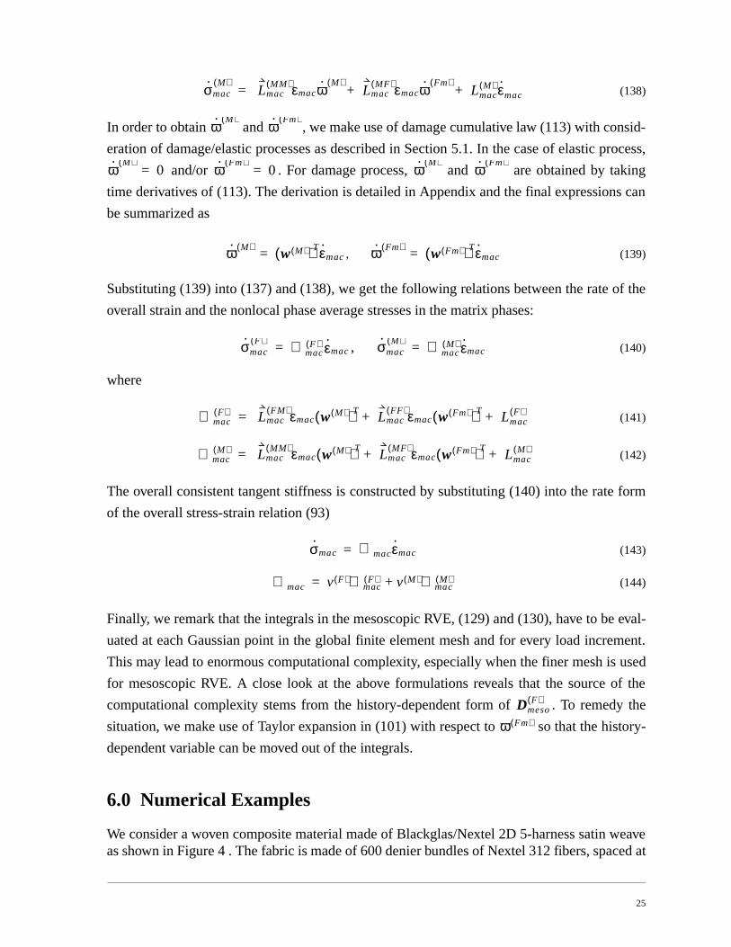
We consider a woven composite material made of Blackglas/Nextel 2D 5-harness satin weaveas shown in Figure 4 . The fabric is made of 600 denier bundles of Nextel 312 fibers, spaced at

σ· macM( )

LmacMM( )εmacω·

M( ) Lmac

MF( )εmacω·Fm( )

LmacM( ) ε·mac+ +=

ω· M( )ω· Fm( )

ω· M( )0= ω· Fm( )

0= ω· M( )ω· Fm( )

ω· M( ) w M( )( )Tε·mac= ω· Fm( ) w Fm( )( )Tε·mac=

σ· macF( ) ℘mac

F( ) ε·mac= σ· macM( ) ℘mac

M( ) ε·mac=

℘macF( ) Lmac

FM( )εmac w M( )( )T LmacFF( )εmac w Fm( )( )T Lmac

F( )+ +=

℘macM( ) Lmac

MM( )εmac w M( )( )T LmacMF( )εmac w Fm( )( )T Lmac

M( )+ +=

σ· mac ℘macε·

mac=

℘mac v F( )℘macF( ) v M( )℘mac

M( )+=

DmesoF( )

ω Fm( )

26

46 threads per inch, and surrounded by Blackglas 493C matrix material. We will refer to thismaterial system as AF10. The micrograph in Figure 4 was produced at Northrop-Gruman.

FIGURE 4. BlackglasTM/Nextel 5-harness Satin Weave

In this set of numerical examples, the mesoscopic RVE is defined as a two-phase material

(bundle/Blackglas 493C), while bundles consist of unidirectional fibrous composite (micro-

scopic RVE). The phase properties of RVEs on both scales are summarized below:

Microscopic (bundle) RVE:

Blackglas 493C Matrix: volume fraction ; Young’s modulus

; Poisson’s ratio .

NextelTM 312 Fiber: volume fraction ; Young’s modulus

; Poisson’s ratio .

Mesoscopic RVE (AF10 woven composite architecture, Figure 4 ):

Blackglas 493C Matrix (with reduce stiffness): volume fraction ; Young’s

modulus ; Poisson’s ratio = .

Bundle: volume fraction ; properties determined by the homogenized stiff-

ness of the microscopic RVE.

Note that the matrix phase in both RVEs is made of the same material. The stiffness reductionof matrix phase in the mesoscopic RVE is due to initial inter-bundle cracks. The parameters of

v Fm( ) 0.733=

E Fm( ) 82.7GPa= 0.26

v Ff( ) 0.267=

E Ff( ) 151.7GPa= 0.24

v M( ) 0.548=

E M( ) 26.2GPa= 0.26

v F( ) 0.452=

27

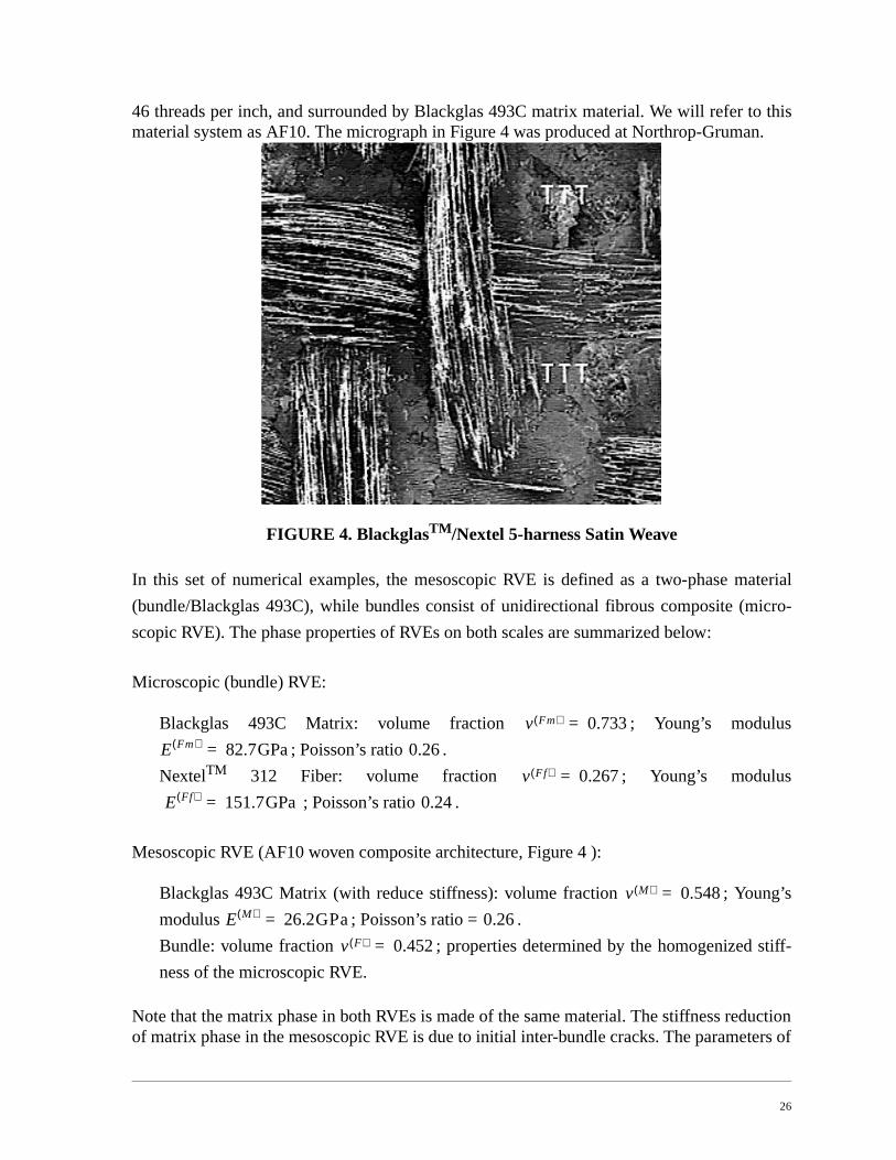
the damage evolution laws are chosen as , and with

. For the matrix phase in the mesoscopic RVE, we choose . For the

matrix phase in the microscopic RVE we define .

We assume that the two matrix phases reach the critical value at the same time under the

equal uniaxial strains, i.e. with

where . The damage evolution laws are depicted

in Figure 5 .

FIGURE 5. Damage Evolution Law on Micro- and Meso- Scales

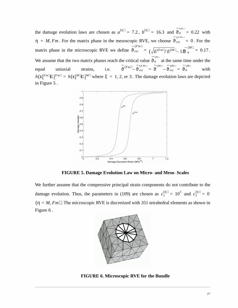
We further assume that the compressive principal strain components do not contribute to the

damage evolution. Thus, the parameters in (109) are chosen as and

. The microscopic RVE is discretized with 351 tetrahedral elements as shown in

Figure 6 .

FIGURE 6. Microscopic RVE for the Bundle

a η( ) 7.2= b η( ) 16.3= ϑ0

η( )0.22=

η M Fm,= ϑini

Fm( )0=

ϑini

Fm( )

E Fm( ) E M( )⁄ 1–( )ϑ0

M( )0.17= =

ϑ0

η( )

ϑ Fm( ) ϑini

Fm( )– ϑ

M( )ϑini

M( )– ϑ0

M( )= =

h εξFm( )( )εξ

Fm( ) h εξM( )( )εξ

M( )= ξ 1 2 or 3, ,=

c1η( ) 105= c2

η( ) 0=

η M Fm,=( )

28

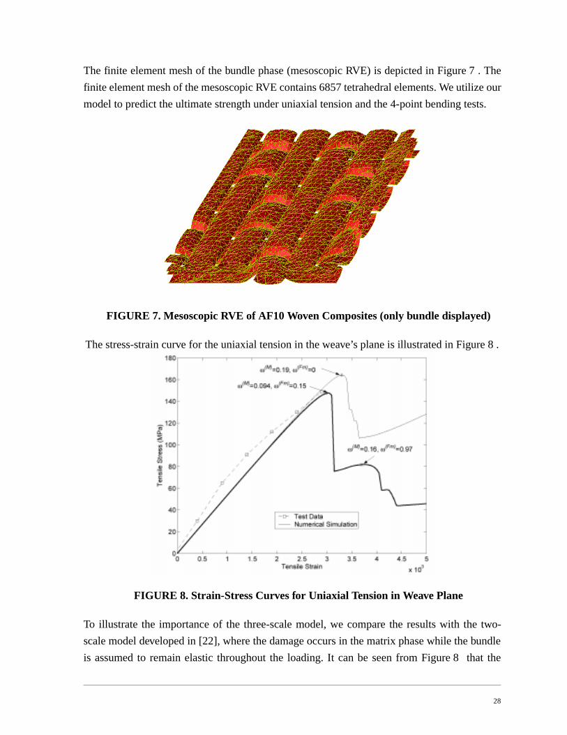
The finite element mesh of the bundle phase (mesoscopic RVE) is depicted in Figure 7 . The

finite element mesh of the mesoscopic RVE contains 6857 tetrahedral elements. We utilize our

model to predict the ultimate strength under uniaxial tension and the 4-point bending tests.

FIGURE 7. Mesoscopic RVE of AF10 Woven Composites (only bundle displayed)

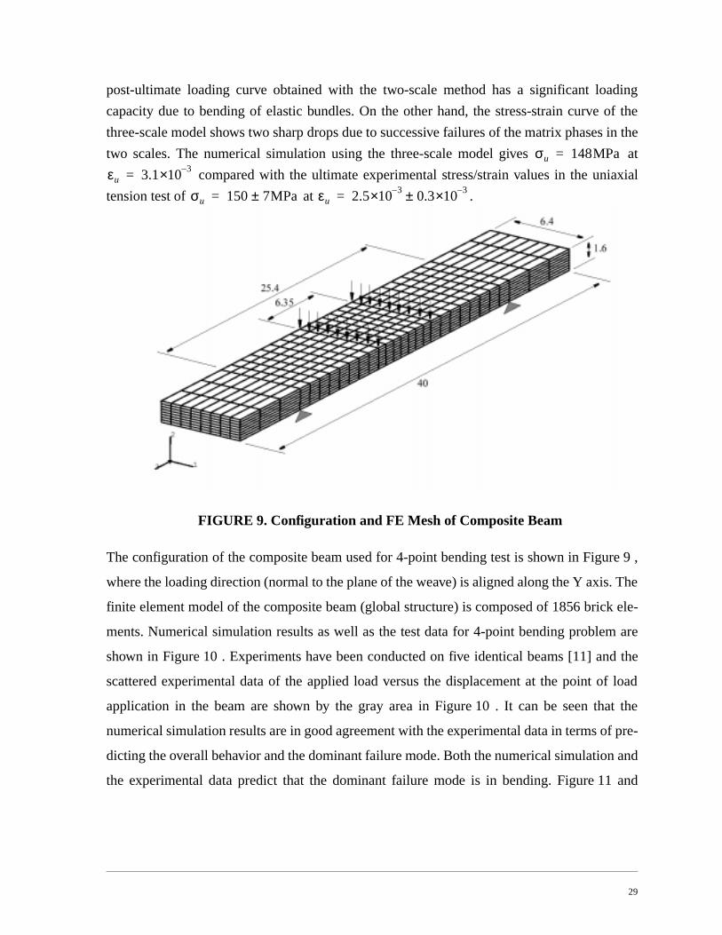
The stress-strain curve for the uniaxial tension in the weave’s plane is illustrated in Figure 8 .

FIGURE 8. Strain-Stress Curves for Uniaxial Tension in Weave Plane

To illustrate the importance of the three-scale model, we compare the results with the two-

scale model developed in [22], where the damage occurs in the matrix phase while the bundle

is assumed to remain elastic throughout the loading. It can be seen from Figure 8 that the

29

post-ultimate loading curve obtained with the two-scale method has a significant loading

capacity due to bending of elastic bundles. On the other hand, the stress-strain curve of the

three-scale model shows two sharp drops due to successive failures of the matrix phases in the

two scales. The numerical simulation using the three-scale model gives at

compared with the ultimate experimental stress/strain values in the uniaxial

tension test of at .

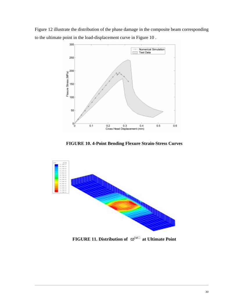
FIGURE 9. Configuration and FE Mesh of Composite Beam

The configuration of the composite beam used for 4-point bending test is shown in Figure 9 ,

where the loading direction (normal to the plane of the weave) is aligned along the Y axis. The

finite element model of the composite beam (global structure) is composed of 1856 brick ele-

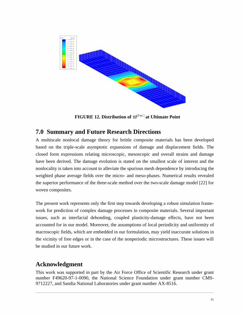
ments. Numerical simulation results as well as the test data for 4-point bending problem are

shown in Figure 10 . Experiments have been conducted on five identical beams [11] and the

scattered experimental data of the applied load versus the displacement at the point of load

application in the beam are shown by the gray area in Figure 10 . It can be seen that the

numerical simulation results are in good agreement with the experimental data in terms of pre-

dicting the overall behavior and the dominant failure mode. Both the numerical simulation and

the experimental data predict that the dominant failure mode is in bending. Figure 11 and

σu 148MPa=

εu 3.1 3–×10=

σu 150 7MPa±= εu 2.5 3–×10 0.3 3–×10±=

30

Figure 12 illustrate the distribution of the phase damage in the composite beam corresponding

to the ultimate point in the load-displacement curve in Figure 10 .

FIGURE 10. 4-Point Bending Flexure Strain-Stress Curves

FIGURE 11. Distribution of at Ultimate Pointω M( )

31

FIGURE 12. Distribution of at Ultimate Point

7.0 Summary and Future Research DirectionsA multiscale nonlocal damage theory for brittle composite materials has been developed

based on the triple-scale asymptotic expansions of damage and displacement fields. The

closed form expressions relating microscopic, mesoscopic and overall strains and damage

have been derived. The damage evolution is stated on the smallest scale of interest and the

nonlocality is taken into account to alleviate the spurious mesh dependence by introducing the

weighted phase average fields over the micro- and meso-phases. Numerical results revealed

the superior performance of the three-scale method over the two-scale damage model [22] for

woven composites.

The present work represents only the first step towards developing a robust simulation frame-

work for prediction of complex damage processes in composite materials. Several important

issues, such as interfacial debonding, coupled plasticity-damage effects, have not been

accounted for in our model. Moreover, the assumptions of local periodicity and uniformity of

macroscopic fields, which are embedded in our formulation, may yield inaccurate solutions in

the vicinity of free edges or in the case of the nonperiodic microstructures. These issues will

be studied in our future work.

AcknowledgmentThis work was supported in part by the Air Force Office of Scientific Research under grantnumber F49620-97-1-0090, the National Science Foundation under grant number CMS-9712227, and Sandia National Laboratories under grant number AX-8516.

ω Fm( )

32

References

1 Allen, D.H., Jones, R.H. and Boyd, J.G. (1994). Micromechanical analysis of a continu-ous fiber metal matrix composite including the effects of matrix viscoplasticity and evolv-ing damage. J. Mech. Phys. Solids 42(3), 505-529.

2 Babuska, I., Anderson, B., Smith, P. and Levin, K. (1999). Damage analysis of fiber com-posites.Part I: Statistical analysis on fiber scale. Comput. Methods Appl.Mech. Engrg. 127,

3 Bakhvalov, A. and Panassenko, G.P., Homogenization: Averaging Processes in PeriodicMedia. Kluwer Academic Publisher, 1989.

4 Bazant, Z.P. (1991). Why continuum damage is nonlocal: micromechanical arguments. J.Engrg. Mech. 117(5), 1070-1087.

5 Bazant, Z.P. and Pijaudier-Cabot, G. (1989). Measurement of characteristic length of non-local continuum. J. Engrg. Mech. 115(4), 755-767.

6 Bazant, Z.P. and Pijaudier-Cabot, G. (1988). Nonlocal continuum damage, localizationinstability and convergence. J. Appl. Mech. 55, 287-293.

7 Belytschko, T., and Lasry, D. (1989). A study of localization limiters for strain softeningin statics and dynamics. Computers and Structures, Vol. 33, pp. 707-715.

8 Belytschko, T., Fish, J. and Engelman, B.E. (1988), “A finite element with embedded localization zones,” Comp. Meth. Appl. Mech. Engrg. 70, 59 - 89.

9 Belytschko, T., and Fish, J. (1989). Embedded hinge lines for plate elements. Comp.Meth. Appl. Mech. Engrg. 76(1), 67-86.

10 Belytschko, T., Fish, J. and Bayliss, A. (1990). The spectral overlay on the finite elementsolutions with high gradients. Comp. Meth. Appl. Mech. Engrg. 81, 71-89.

11 Butler, E.P., Danforth, S.C., Cannon, W.R. and Ganczy, S.T. (1996). Technical Report forthe ARPA LC3 program, ARPA Agreement No. MDA 972-93-0007.

12 Chaboche, J.L. (1988). Continuum damage mechanics I: General concepts. J. Appl. Mech.55, 59-64.

13 deVree, G.H.P., Brekelmans, W.A.J. and Van Gils, M.A.J. (1995). Comparison of nonlo-cal approaches in continuum damage mechanics. Comput. Structures. 55(4), 581-588.

14 Fish, J. and Belytschko, T. (1988). Elements with embedded localization zones for largedeformation problems. Computers and Structures 30(1/2), 247-256.

15 Fish, J. and Belytschko, T. (1990). A finite element with a unidirectionally enrichedstrain field for localization analysis. Comp. Meth. Appl. Mech. Engrg. 78(2), 181-200.

16 Fish, J. and Belytschko, T. (1990). A general finite element procedure for problems withhigh gradients. Computers and Structures 35(4), 309-319.

17 Fish, J. and Belsky, V. (1995). Multigrid method for a periodic heterogeneous medium.Part I: Convergence studies for one-dimensional case. Comp. Meth. Appl. Mech. Engrg.

33

126, 1-16.

18 Fish, J. and Belsky, V. (1995). Multigrid method for a periodic heterogeneous medium.Part 2: Multiscale modeling and quality control in multidimensional case. Comp. Meth.Appl. Mech. Engrg. 126, 17-38.

19 Fish, J., Nayak, P. and Holmes, M.H. (1994). Microscale reduction error indicators andestimators for a periodic heterogeneous medium. Comput. Mech. 14, 323-338.

20 Fish, J., Shek, K., Pandheeradi, M., and Shephard, M.S. (1997). Computational plasticityfor composite structures based on mathematical homogenization: Theory and practice.Comput. Meth. Appl. Mech. Engrg. 148, 53-73.

21 Fish, J. and Wagiman, A. (1993). Multiscale finite element method for locally nonperi-odic heterogeneous medium. Comput. Mech. 12, 164-180.

22 Fish, J. and Yu, Q. and Shek, K. (1999). Computational damage mechanics for compositematerials based on mathematical homogenization. Int. J. Num. Methods in Engrg. 45,1657-1679

23 Fish, J., and Yu, Q. (2000). Computational mechanics of fatigue and life predictions forcomposite materials and structures, submitted to Comp. Meth. Appl. Mech. Engrg.

24 Geers, M.G.D., Experimental and Computational Modeling of Damage and Fracture.Ph.D Thesis. Technische Universiteit Eindhoven, The Netherlands, 1997.

25 Geers, M.G.D., Peerlings, R.H.J., de Borst, R. and Brekelmans, W.A.M. (1998), Higher-order damage models for the analysis of fracture in quasi-brittle materials, In: MaterialInstabilities in Solids, (Edited by R. deBorst and E. van der Giessen), pp 405~423, JohnWiley & Sons, Chichester, UK.

26 Guedes, J.M. and Kikuchi, N. (1990). Preprocessing and postprocessing for materials based on the homogenization method with adaptive finite element methods. Comput. Methods Appl. Mech. Engrg. 83, 143-198.

27 Ju, J.W. (1989) On energy-based coupled elastoplastic damage theories: Constitutivemodeling and computational aspects. Int. J. Solids Structures 25(7), 803-833.

28 Krajcinovic, D. (1996). Damage Mechanics. Elsevier Science.

29 Kruch, S., Chaboche, J. L. and Pottier, T. (1996). Two-scale viscoplastic and damageanalysis of metal matrix composite. In: Damage and Interfacial Debonding in Composites(Edited by G. Z. Voyiadjis and D. H. Allen), pp. 45-56, Elsevier Science.

30 Ladeveze, P. and Le-Dantec, E. (1992). Damage modeling of the elementary ply for lami-nated composites. Composites Science and Technology. 43, 257-267.

31 Lee, K., Moorthy, S. and Ghosh, S. (1999). Multiple-scale adaptive computational modelfor damage in composite materials”. Comput. Methods Appl. Mech. Engrg.

32 Lemaitre, J (1984). How to use damage mechanics. Nucl. Engrg. Design. 80, 233-245

33 Lene, F. (1986). Damage constitutive relations for composite materials. Engrg. Fract.

34

Mech. 25, 713-728.

34 Matzenmiller, A., Lubliner, J. and Taylor, R.L. (1995). A constitutive model for anisotro-pic damage in fiber-composites. Mech. Mater. 20, 125-152

35 Oden, J.T., Vemaganti, K. and Mo s, N. (1998). Hierarchical modeling of heterogeneoussolids. Special Issue of Comput. Methods Appl. Mech. Engrg. on Computational Advancesin Modeling Composites and Heterogeneous Materials (edited by J. Fish).

36 Oden, J.T. and Zohdi, T.I. (1996). Analysis and adaptive modeling of highly heteroge-neous elastic structures, TICAM Report 56, University of Texas at Austin.

37 Peerling, R.H.J., de Borst, R., Brekelmans, W.A.M. and de Vree, J.H.P. (1996). Gradientenhanced damage for quasi-brittle materials. Int. J. Num. Methods Engrg. 39, 3391-3403.

38 Simo, J.C. and Ju, J.W. (1987) Strain- and stress-based continuum damage models - I.Formulation. Int. J. Solids Structures 23(7), 821-840.

39 Talreja, R. (1989). Damage development in composite: Mechanism and modeling. J.Strain Analysis 24, 215-222.

40 Voyiadjis, G.Z. and Park, T. (1992). A plasticity-damage theory for large deformation ofsolids-I: Theoretical Formulation. Int. J. Engrg. Sci. 30(9), 1089-1106.

41 Voyiadjis, G.Z. and Kattan, P. (1993). Micromechanical characterization of damage-plas-ticity in metal matrix composites. In: Damage in Composite Materials (Edited by G. Z.Voyiadjis), pp67-102, Elsevier Science.

42 Voyiadjis, G.Z. and Park, T.(1996). Elasto-plastic stress and strain concentration tensorsfor damaged fibrous composites. In: Damage and Interfacial Debonding in Composites(Edited by G. Z. Voyiadjis and D. H. Allen), pp81-106, Elsevier Science.

43 Wentorf, R., Collar, R., Shephard, M.S. and Fish, J. (1999). Automated Modeling for complex woven mesostructures, Comput. Methods Appl. Mech. Engrg. 172, 273-291.

Appendix

In this section we present detailed derivations for in (117) and

(118), and in (139). We start with the first derivative by differentiating (107) with respect

to

(A1)

where the vector takes following form

(A2)

e··

ϑ λ( ) ω η( )∂⁄∂ λ η, M Fm,=

ω· η( )

ω λ( )

ϑη( )

∂ω λ( )∂

------------ e η( )( )T F η( )εmac

η( )( )∂

ω λ( )∂---------------------------- λ η, M Fm,=,=

e η( ) e1η( ) e2

η( ) e3η( ), ,[ ]T≡

e η( )( )T 1

2ϑm( )------------- F η( )εmac

η( )( )

TLmac

η( )=

35

With the definition of in (108), the derivative in (A1) can be expressed as

(A3)

Since the three components of the vector in (A3) have a similar form, we simply denote them

by with and then by using (109) we have

(A4)

where

(A5)

To this end we need to compute the derivative of each component of principal strain with

respect to the damage variable . The principal components of a second order tensor sat-

isfy Hamilton’s Theorem, i.e.

(A6)

where and are three invariants of (or ) which can be expressed as

(A7)

(A8)

(A9)

where the tensorial notations are adopted for , i.e . Differentiating (A6) with

respect to gives

(A10)

F η( )

F η( )εmacη( )( )∂

ω λ( )∂---------------------------- h1

η( )ε1η( )( )∂

ω λ( )∂-------------------------

h2η( )ε2

η( )( )∂ω λ( )∂

------------------------- h3

η( )ε3η( )( )∂

ω λ( )∂-------------------------

T

=

hξη( )εξ

η( )( ) ω λ( )∂( )⁄∂ ξ 1 2 3, ,=

hξη( )εξ

η( )( )∂

ω λ( )∂-------------------------

hξη( )∂

εξη( )

∂----------- εξ

η( )hξ

η( )+ εξ

η( )∂ω λ( )∂

------------ ; ξ 1 2 3, ,==

hξη( )∂

εξη( )

∂-----------

c1η( ) π⁄

1 c1η( ) εξ

η( )c2

η( )–( ) 2+

-------------------------------------------------------=

εmacη( )

ω λ( )

εξη( )

( )3

I1 εξη( )

( )2

– I2εξη( )

I3–+ 0=

I1 I2, I3 εmacη( ) εmac

η( )

I1 εi iη( ) ε1

η( )ε2

η( )ε3

η( )+ += =

I212--- εi i

η( )εj jη( ) εi j

η( )εj iη( )–( )⋅ ε1

η( )ε2

η( )ε2

η( )ε3

η( )ε3

η( )ε1

η( )+ += =

I316--- 2εi j

η( )εjkη( )εki

η( ) 3εi jη( )εj i

η( )εkkη( )– εi i

η( )εj jη( )εkk

η( )+( )⋅ ε1η( )

ε2η( )

ε3η( )

= =

εmacη( ) εmac

η( ) εi jη( )≡

ω λ( )

εξη( )

∂ω λ( )∂

------------ 3 εξη( )

( )2

2I1εξη( )

– I2+ 1– I∂ 1

ω λ( )∂------------ εξ

η( )( )

2 I∂ 2

ω λ( )∂------------ εξ

η( )–

I∂ 3

ω λ( )∂------------+

⋅=

36

where the derivative of the invariants with respect to can be obtained by using (A7)-(A9)

such that

(A11)

(A12)

(A13)

Substituting (A10)-(A13) into (A4), gives

(A14)

where is given as

(A15)

Finally, in (A1) can be written in a concise form by using (A3) and (A14),

which yields

(A16)

where

(A17)

and the derivative on right hand side of (A16) can be evaluated by differentiating (111) and

(112) such that

(A18)

ω λ( )

I∂ 1

ω λ( )∂------------ p1

η( )( )T εmac

η( )∂ω λ( )∂

-------------≡ δ jkδik

εi jη( )∂

ω λ( )∂------------=

I∂ 2

ω λ( )∂------------ p2

η( )( )T εmac

η( )∂ω λ( )∂

-------------≡ εmmη( ) δjkδik εj i

η( )–( )εi j

η( )∂ω λ( )∂

------------=

I∂ 3

ω λ( )∂------------ p3

η( )( )T εmac

η( )∂ω λ( )∂

-------------

≡

εjkη( )εki

η( ) εmmη( ) εj i

η( )–12---εmn

η( )εnmη( )δjkδik

12---εmm

η( ) εnnη( )δjkδik+–

εi jη( )∂

ω λ( )∂------------=

hξη( )εξ

η( )( )∂

ω λ( )∂------------------------- qξ

η( )( )T εmac

η( )∂ω λ( )∂

------------- , ξ 1 2 3, ,==

qξη( )

qξη( ) hξ

η( )∂

εξη( )

∂----------- εξ

η( )hξ

η( )+

3 εξη( )

( )2

2I1εξη( )

– I2+ 1–

p1η( ) εξ

η( )( )

2p2

η( )εξη( )

– p3η( )+ =

ϑη( )

ω λ( )∂⁄∂

ϑη( )

∂ω λ( )∂

------------ ℵ η( )( )T

εmacη( )∂

ω λ( )∂-------------

λ η, M Fm,=,=

ℵ η( ) eξη( )qξ

η( )

ξ 1=

3

∑ η M Fm,=,=

εmacM( )d s1

M( ) ω M( )d s2M( ) ω Fm( )d S M( ) εmacd+ +=

37

(A19)

where for (A18)

(A20)

(A21)

(A22)

and for (A19)

(A23)

(A24)

(A25)

The time derivatives of the phase damage variable, and , can be obtained by taking

time derivatives of damage evolution law (113) and making use of (A18) and (A19). From

(113) and assuming that damage processes occur on both scales, i.e.

, we have

(A26)

(A27)

where and are given in (119); and can be derived in a similar way as

for , which yields:

(A28)

εmacFn( )d s1

F( ) ω M( )d s2F( ) ω Fm( )d S F( ) εmacd+ +=

εmacM( )∂

ω M( )∂------------- s1

M( )≡ GyM( )Dmac

M( ) εmac=

εmacM( )∂

ω Fm( )∂---------------- s2

M( )≡ GyM( )Dmac

F( ) εmac=

εmacM( )∂

εmac∂------------- S M( )≡ Ay

M( ) GyM( )Dmac+=

εmacFm( )∂

ω M( )∂--------------- s1

Fm( )≡ 1

ΘyF( )

------------- AzFm( ) Gz

Fm( )DmesoF( )+( )GyDmac

M( ) Θ εmacdΘy

F( )∫=

εmacFm( )∂

ω Fm( )∂---------------- s2

Fm( )≡ 1

ΘyF( )

------------- GzFm( )

DmesoF( )

Ay GyDmac+( )

AzFm( )

GzFm( )

DmesoF( )+( )GyDmac

F( )+

Θd

ΘyF( )∫

εmac

=

εmacFm( )∂

εmac∂--------------- S Fm( )≡ 1

ΘyF( )

------------- AzFm( ) Gz

Fm( )DmesoF( )+( ) Ay GyDmac+( ) Θd

ΘyF( )∫=

ω· M( ) ω· Fm( )

κ η( ) ϑ η( )=

η M Fm,=( )

ω· M( ) γ M( )ϑ· M( )

=

ω· Fm( ) γ Fm( )ϑ· Fm( )

=

γ M( ) γ Fm( ) ϑ· M( )

ϑ· Fm( )

ϑη( )

ω λ( )∂⁄∂

ϑ· η( )

ℵ η( )( )Tε·macη( )

η M Fm,=,=

38

where can be evaluated by using (A18) and (A19). From (A26) and (A18), we can get

(A29)

where and are given as

(A30)

(A31)

(A32)

Similarly, from (A28) and (A19), we have

(A33)

where and are given as

(A34)

(A35)

(A36)

Finally, solving for (A29) and (A33) yields

, (A37)

where

(A38)

(A39)

The Jacobian matrix (116)-(118) follows from (A16), (A20), (A21), (A23), (A24), (A30),

(A31), (A34) and (A35):

(A40)

ε·macη( )

n1M( )ω· M( ) n2

M( )ω· Fm( )r M( )( )Tε·mac+ + 0=

n1M( ) n2

M( ), r M( )

n1M( ) ℵ M( )( )T

s1M( ) 1 γ M( )⁄–=

n2M( ) ℵ M( )( )T

s2M( )=

r M( )( )T ℵ M( )( )TS M( )=

n1Fm( )ω· M( ) n2

Fm( )ω· Fm( )r Fm( )( )Tε·mac+ + 0=

n1Fm( ) n2

Fm( ), r Fm( )

n1Fm( ) ℵ Fm( )( )T

s1Fm( )=

n2Fm( ) ℵ Fm( )( )T

s2Fm( ) 1 γ Fm( )⁄–=

sFm( )( )T ℵ Fm( )( )TS Fm( )=

ω· M( ) w M( )( )Tε·mac= ω· Fm( ) w Fm( )( )Tε·mac=

w M( ) n2M( )r Fm( ) n2

Fm( )r M( )–

n1M( )n2

Fm( ) n2M( )n

1Fm( )–

--------------------------------------------------=

w Fm( ) n1Fm( )r M( ) n1

M( )r Fm( )–

n1M( )n2

Fm( ) n2M( )n

1Fm( )–

--------------------------------------------------=

Jγ M( )n1

M( ) γ M( )n2M( )

γ Fm( )n1Fm( ) γ Fm( )n2

Fm( )=