JID:PLREV AID:465 /REV [m3SC+; v 1.188; Prn:4/03/2014; 13:24] P.1(1-59) Available online at www.sciencedirect.com ScienceDirect Physics of Life Reviews ••• (••••) •••–••• www.elsevier.com/locate/plrev Review Multiscale approach to pest insect monitoring: Random walks, pattern formation, synchronization, and networks Sergei Petrovskii a,∗ , Natalia Petrovskaya b , Daniel Bearup a a Department of Mathematics, University of Leicester, University Road, Leicester LE1 7RH, UK b School of Mathematics, University of Birmingham, Birmingham B15 2TT, UK Received 18 July 2013; accepted 4 February 2014 Communicated by J. Fontanari Abstract Pest insects pose a significant threat to food production worldwide resulting in annual losses worth hundreds of billions of dollars. Pest control attempts to prevent pest outbreaks that could otherwise destroy a sward. It is good practice in integrated pest management to recommend control actions (usually pesticides application) only when the pest density exceeds a certain threshold. Accurate estimation of pest population density in ecosystems, especially in agro-ecosystems, is therefore very important, and this is the overall goal of the pest insect monitoring. However, this is a complex and challenging task; providing accurate information about pest abundance is hardly possible without taking into account the complexity of ecosystems’ dynamics, in particular, the existence of multiple scales. In the case of pest insects, monitoring has three different spatial scales, each of them having their own scale-specific goal and their own approaches to data collection and interpretation. In this paper, we review recent progress in mathematical models and methods applied at each of these scales and show how it helps to improve the accuracy and robustness of pest population density estimation. © 2014 Elsevier B.V. All rights reserved. Keywords: Insect monitoring; Trapping; Diffusion; Levy walk; Numerical integration; Dispersal Contents 1. Introduction ......................................................................... 2 2. Single trap problem .................................................................... 4 2.1. Individual-based approach ........................................................... 4 2.2. Mean-field approach: Diffusion equation ................................................. 10 2.3. Boundary forcing ................................................................. 19 2.4. Random walk of non-identical dispersers ................................................. 22 2.5. Trapping of Levy-walking insects: time-dependent diffusion as an alternative framework? ................ 25 * Corresponding author. http://dx.doi.org/10.1016/j.plrev.2014.02.001 1571-0645/© 2014 Elsevier B.V. All rights reserved.

Welcome message from author
This document is posted to help you gain knowledge. Please leave a comment to let me know what you think about it! Share it to your friends and learn new things together.
Transcript
JID:PLREV AID:465 /REV [m3SC+; v 1.188; Prn:4/03/2014; 13:24] P.1 (1-59)
Available online at www.sciencedirect.com
ScienceDirect
Physics of Life Reviews ••• (••••) •••–•••www.elsevier.com/locate/plrev
Review
Multiscale approach to pest insect monitoring: Random walks,pattern formation, synchronization, and networks
Sergei Petrovskii a,∗, Natalia Petrovskaya b, Daniel Bearup a
a Department of Mathematics, University of Leicester, University Road, Leicester LE1 7RH, UKb School of Mathematics, University of Birmingham, Birmingham B15 2TT, UK
Received 18 July 2013; accepted 4 February 2014
Communicated by J. Fontanari
Abstract
Pest insects pose a significant threat to food production worldwide resulting in annual losses worth hundreds of billions ofdollars. Pest control attempts to prevent pest outbreaks that could otherwise destroy a sward. It is good practice in integrated pestmanagement to recommend control actions (usually pesticides application) only when the pest density exceeds a certain threshold.Accurate estimation of pest population density in ecosystems, especially in agro-ecosystems, is therefore very important, and thisis the overall goal of the pest insect monitoring. However, this is a complex and challenging task; providing accurate informationabout pest abundance is hardly possible without taking into account the complexity of ecosystems’ dynamics, in particular, theexistence of multiple scales. In the case of pest insects, monitoring has three different spatial scales, each of them having theirown scale-specific goal and their own approaches to data collection and interpretation. In this paper, we review recent progress inmathematical models and methods applied at each of these scales and show how it helps to improve the accuracy and robustnessof pest population density estimation.© 2014 Elsevier B.V. All rights reserved.
Keywords: Insect monitoring; Trapping; Diffusion; Levy walk; Numerical integration; Dispersal
Contents
1. Introduction . . . . . . . . . . . . . . . . . . . . . . . . . . . . . . . . . . . . . . . . . . . . . . . . . . . . . . . . . . . . . . . . . . . . . . . . . 22. Single trap problem . . . . . . . . . . . . . . . . . . . . . . . . . . . . . . . . . . . . . . . . . . . . . . . . . . . . . . . . . . . . . . . . . . . . 4
2.1. Individual-based approach . . . . . . . . . . . . . . . . . . . . . . . . . . . . . . . . . . . . . . . . . . . . . . . . . . . . . . . . . . . 42.2. Mean-field approach: Diffusion equation . . . . . . . . . . . . . . . . . . . . . . . . . . . . . . . . . . . . . . . . . . . . . . . . . 102.3. Boundary forcing . . . . . . . . . . . . . . . . . . . . . . . . . . . . . . . . . . . . . . . . . . . . . . . . . . . . . . . . . . . . . . . . . 192.4. Random walk of non-identical dispersers . . . . . . . . . . . . . . . . . . . . . . . . . . . . . . . . . . . . . . . . . . . . . . . . . 222.5. Trapping of Levy-walking insects: time-dependent diffusion as an alternative framework? . . . . . . . . . . . . . . . . 25
* Corresponding author.
http://dx.doi.org/10.1016/j.plrev.2014.02.0011571-0645/© 2014 Elsevier B.V. All rights reserved.

JID:PLREV AID:465 /REV [m3SC+; v 1.188; Prn:4/03/2014; 13:24] P.2 (1-59)
2 S. Petrovskii et al. / Physics of Life Reviews ••• (••••) •••–•••
3. Single field problem: multiple traps . . . . . . . . . . . . . . . . . . . . . . . . . . . . . . . . . . . . . . . . . . . . . . . . . . . . . . . . . . 303.1. Evaluation of pest insect abundance from discrete data . . . . . . . . . . . . . . . . . . . . . . . . . . . . . . . . . . . . . . . . 313.2. Evaluation of population abundance on coarse grids . . . . . . . . . . . . . . . . . . . . . . . . . . . . . . . . . . . . . . . . . . 343.3. Integration of high-aggregation density distributions . . . . . . . . . . . . . . . . . . . . . . . . . . . . . . . . . . . . . . . . . 40
4. Landscape scale: synchronization and self-organization . . . . . . . . . . . . . . . . . . . . . . . . . . . . . . . . . . . . . . . . . . . . 425. Discussion . . . . . . . . . . . . . . . . . . . . . . . . . . . . . . . . . . . . . . . . . . . . . . . . . . . . . . . . . . . . . . . . . . . . . . . . . . 50
Acknowledgements . . . . . . . . . . . . . . . . . . . . . . . . . . . . . . . . . . . . . . . . . . . . . . . . . . . . . . . . . . . . . . . . . . . . . . . . . 54References . . . . . . . . . . . . . . . . . . . . . . . . . . . . . . . . . . . . . . . . . . . . . . . . . . . . . . . . . . . . . . . . . . . . . . . . . . . . . . . 54
1. Introduction
The structure and functioning of ecosystems have long been paradigms of complexity [26,86]. In particular, ithas been increasingly recognized that ecosystem properties arise as a result of coupling between processes goingon different spatial scales [61,75,84,169]. The notion of multiple scales applies to virtually all aspects of ecosystemfunctioning and to ecosystem monitoring, in particular, to pest insect monitoring. Pest monitoring is an issue of hugepractical importance, especially in agricultural ecosystems or ‘agro-ecosystems’. Indeed, pests are a sustained andsignificant problem in the production of food across the globe. Crops are vulnerable to attack from pests both duringthe growing process and after they have been harvested. Estimates of the annual worldwide loss due to pests at thepre-harvest stage lie between 35 and 42% [106,133]. In particular, the pre-harvest loss of 14–15% of the world’s cropshas been attributed to harmful insects [136,134].
Effective and reliable ecological monitoring is required in order to provide detailed and timely information aboutpest species. In agro-ecosystems, monitoring is usually a part of the integrated pest management (IPM) [28,82]. Thebasic principle of the IPM is that a control action is only used if and when it is necessary. The decision of whether ornot to implement a control action is made by comparing the abundance of pests against some threshold level, i.e. thelimit at which intervening becomes worth the effort and expense. Such threshold values can be decided upon by takinga variety of factors into consideration. Economic thresholds are most commonly used [162] as the overriding concernis that the pest management program is financially viable (e.g. see [63]).
Once the pest abundance exceeds the threshold, the IPM decision is to intervene and implement a control action,usually application of chemical pesticides. However, use of chemical pesticides has many drawbacks. The first ofthese is the damage caused to the environment. It has been estimated that around 3 · 109 kg are used across the globeper year [134]. As a result, pesticides significantly contribute to air, soil and water pollution, and there is growingevidence linking their use to human illnesses [4,135]. Note that the per capita efficiency of chemical pesticides isestimated to be quite low as, on average, less than 0.1% of them reach their targeted pest [132].
Secondly, use of chemical pesticides results in significant additional costs added to the agricultural product. Indeed,it is estimated that around $40 billion per year is spent on pesticides [134]. Hence a reduction in the amount ofpesticides used would be clearly desirable from the economic perspective.
Finally, indiscriminate or preemptive use of pesticides can make them less efficient. For instance, regular use ofpesticides can result in the pest becoming resistant, thus making future management a more difficult task [8]. Anotherunwanted side effect is that the pesticide can have lethal or sub-lethal effects on natural enemies [157] which cancause a resurgence in the pest population or a secondary pest to emerge.
Thus, accurate monitoring is key to the decision process [28,92]. There is an urgent need for reliable methods toestimate the pest population size in order to avoid unjustified pesticides application and yet to prevent pest outbreaks.In this paper, we review some of the recent research in pest monitoring models and methods applied on differentspatial scales.
Two essential components of monitoring are data collection and data processing and/or interpretation. These are notindependent as a reliable estimate of the population density resulting from data processing can only be obtained if thecollected data contain sufficient information. The latter can be achieved if the spatial arrangement of the data is madeconsistent with the spatial structure of the agro-ecosystem as given by the self-organized spatiotemporal patterns inthe pest species distribution and by the environmental forcing through heterogeneous landscape and weather patterns.
JID:PLREV AID:465 /REV [m3SC+; v 1.188; Prn:4/03/2014; 13:24] P.3 (1-59)
S. Petrovskii et al. / Physics of Life Reviews ••• (••••) •••–••• 3
A common method to collect field data regarding insect abundance is trapping. A number of traps are installedacross the monitored area, e.g. in a field or grassland. They are emptied on a regular basis, their content is analyzed,different species identified and counted. The trap counts are then used to estimate the population density of harmfulspecies at the positions of the traps. Correspondingly, there are three basic spatial scales in the pest monitoring prob-lem. The research approaches depend on the spatial scale where the data are collected, and in this paper we discussrelevant physical/biological mechanisms and an adequate mathematical framework for each spatial scale involved.
The first and smallest spatial scale is related to a single trap. The relevant biological process is individual insectmovement and the corresponding theoretical framework is a random walk [127]. The main challenge here is to sep-arate the effects of population density from the effects of movement,1 in particular, to reveal how the trap counts(and, consequently, the estimate of population density in the vicinity of the trap) may be affected by the type ofstochastic process, i.e. whether it is Brownian motion or a Levy flight. The problem is made more difficult by theinherent stochastic variation of individual traits that sometimes can make it impossible to distinguish between Brow-nian motion and Levy flights [124]. Also, the presence of other movement modes (cf. “composite Brownian motion”)or the discretization of continuous individual movement on an inadequate time-scale may result in “superficial Levyflights” [69,78].
The next spatial scale arises when the information about pest density obtained at several different locations(e.g. from several traps) has to be used in order to estimate the average pest density over a certain area, e.g. overa large agricultural field. A standard approach used in ecology is based on calculating the arithmetic average of localdensities. This approach, although efficient in the case of an approximately uniform spatial population distribution,becomes ineffective and inaccurate if the distribution is heterogeneous, e.g. due to pattern formation. However, patternformation in ecological populations is a phenomenon commonly seen in ecological data [47] and explained by well-developed theories [110,88]. To address this, a new approach to estimate the average population density from sparsediscrete spatial data (e.g. trap counts collected in the nodes of a spatial grid) has recently been developed [116,117]and was shown to be effective even in case of very coarse spatial data and a very patchy population distribution [119].In the case of ‘extreme aggregation’, i.e. where the population density forms a sharp narrow peak, it was shown thatthe system attains probabilistic properties: the average population density becomes a stochastic variable and the sys-tem is quantified by the probability that its value lies in a pre-defined range [44]. A general conclusion is that, at thisspatial scale, a robust estimate of the population size can be possible even on a very coarse grid if some properties ofthe population distribution are known, thus linking this problem to the problem of pattern formation [118].
The largest spatial scale in the problem of pest monitoring is the landscape scale that may include many agriculturalfields as well as non-farmed habitats and non-agricultural areas. The main problems here are to reveal long-distancecross-correlations between the pest abundance in different fields or habitats, the phenomenon known as synchroniza-tion, and to identify the mechanisms resulting in synchronization. Two main mechanisms that can synchronize thepopulation dynamics in different fields are known to be coupling by inter-habitat dispersal and the effect of spatiallycorrelated noise. Whilst synchronization by noise is usually isotropic, synchronization by dispersal can exhibit cleardirectional preference [15]. Having revisited some recent results, we show that dispersal between different habitatscan occur through a certain self-organized network. Such a network can arise as a result of the interplay betweenlandscape properties, weather conditions and the behavioral response of the dispersing insects. As a result, close fieldscan be virtually uncorrelated but some fields as far away from each other as a few hundred kilometers can be almostperfectly synchronized.
The paper is structured according to the three spatial scales outlined above; see Sections 2 to 4, respectively. Afterthe scale-specific problems and research approaches are discussed, we then consider the coupling between these scales(Section 5). In particular, we discuss how the processes acting on these different spatial scales can be related, whatare the mechanisms and the relevant modeling approaches, and how the information obtained on one scale can betranslated to the other scales in order to increase the robustness and effectiveness of pest insect monitoring acrossspatial scales.
1 This problem is also known as the “activity-density paradigm” [165]: clearly, a similar increase in the trap counts may result either from anincrease in the pest population density or from an increase in the intensity of the individual movement.
JID:PLREV AID:465 /REV [m3SC+; v 1.188; Prn:4/03/2014; 13:24] P.4 (1-59)
4 S. Petrovskii et al. / Physics of Life Reviews ••• (••••) •••–•••
2. Single trap problem
In pest insect monitoring, as well as in insect studies in general, information about the local abundance of a givenspecies is usually obtained by installing traps and analyzing trap counts. Depending on the traits of the target species,the traps can be of different designs. In the case of walking or crawling insects, a trap is essentially just a hole in theground, often with a cup or bowl inserted inside in order to make it easier to empty. They can be of different shape.Traps of a circular shape are most common, although a variety of other shapes and design are used as well [130,49].The size of the trap is usually much larger (by the factor of ∼102) than the typical body size of the monitored insects.Traps are escape-proof; once an insect gets inside, it is held captive and is eventually killed. Also, traps can be eitherbaited, i.e. using a certain agent that attracts insects to the trap such as light or pheromone, or non-baited. Becausebaited traps alter the insect behavior, they are much more difficult to model and the corresponding theory is largelyabsent. Here we mostly consider non-baited traps.
In this section, we revisit two different (albeit related) approaches to trap counts modeling and interpretation: theindividual-based approach, where the movement of each individual is followed explicitly, and the mean-field approach,where trap counts are described in term of the population density in the vicinity of the trap. We will show that, in orderto achieve a good understanding of trap counts, the two approaches should be used together.
Interpretation of trap counts aiming to estimate the population abundance in the vicinity of a trap is not at allstraightforward. The essence of the challenge is readily seen from the following example. Consider a trap of radius r
that has caught C1 insects after having been exposed for time T . This simple situation brings to the fore a number ofquestions concerning whether we can obtain the population density U0 from this information. (i) If this information issufficient, how do we actually calculate U0? (ii) If this information is insufficient, then what else (e.g. how many morecounts) do we need to know in order to get a reasonably accurate estimate of the population density? (iii) How theadditional information can be used in order to improve the accuracy of the estimate? Further in the text, we will referto it as the ‘single trap problem’. Existing semi-empirical approaches suggest that U0 = κC1/(DT ) where D is thediffusion coefficient and κ is a certain numerical coefficient, thus regarding DT as the effective ‘catchment area’ [30,165]. However, this approach does not work in the case of repeated trap counts because it does not take into accountthe perturbation to the spatial distribution of the insects introduced by the trap. Moreover, a consistent theory androbust computational algorithms only exist in the case where insects perform Brownian motion. There is increasingevidence that animals may perform non-Brownian motion such as Levy flights, but a theory relating the correspondingtrap counts to population density is lacking. Note that the problem of trapping has been studied extensively in physics(e.g. see [50]) including the case of anomalous diffusion [93], but most of the studies are concerned with large-timeasymptotics while for insect monitoring short-time dynamics is of primary interest.
2.1. Individual-based approach
It is common knowledge that animals move in space. Such motion is regarded as an essential feature of animal life.Through their individual movement, animals make better use of the environment, e.g. by foraging, by searching fora mating partner, by avoiding predators, etc. Once a trap is installed, it introduces a perturbation into the movement;when an animal (e.g. insect) encounters the trap on its way, it will fall into it with a certain probability. This probabilitycan depend on the trap design (e.g. it is larger for baited traps than for non-baited ones) and on the species traits. Forwell-designed traps, it is close to one, and this is what we are going to assume throughout the text without a loss ofgenerality.
Before the animal will have a chance to fall into the trap, it has to get close to the trap boundary. Therefore, wefirst need to consider the movement in a more formal way. For the sake of clarity, here we focus on movement intwo spatial dimensions, i.e. in the plane (x, y). Our analysis therefore immediately applies to trapping of walking orcrawling insects in a field. Reduction of the approach to a simpler 1D case or its extension onto a slightly more general3D case are relatively straightforward.
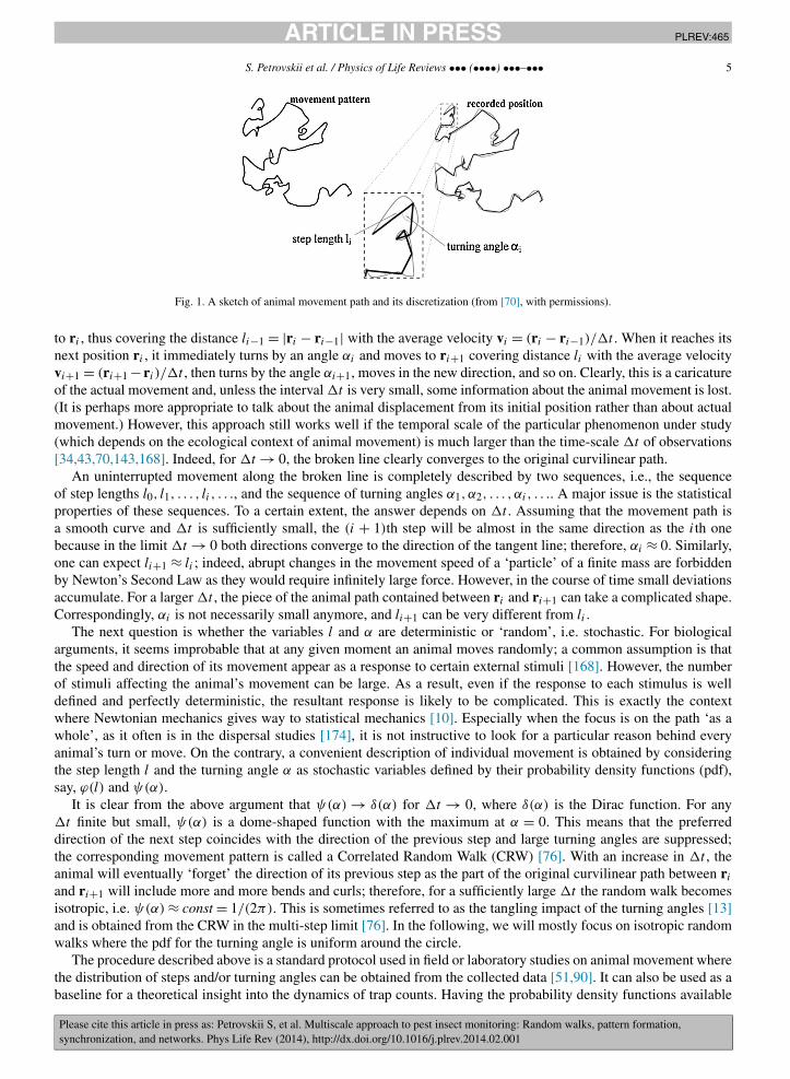
Generally, movement of an individual animal takes place along a certain curvilinear path or trajectory. In obser-vations, the animal’s position is usually recorded not continuously but at certain moments (say, t0, t1, . . . , ti , . . .), forinstance, by taking snapshots of the movement arena. Correspondingly, the curvilinear path is mapped into a brokenline defined by the positions ri = r(ti), i = 0,1, . . . , of the animal [168]; see Fig. 1. For the sake of simplicity, weassume that ti+1 − ti = �t = const for all i. Over the interval �t , the animal moves along the straight line from ri−1
JID:PLREV AID:465 /REV [m3SC+; v 1.188; Prn:4/03/2014; 13:24] P.5 (1-59)
S. Petrovskii et al. / Physics of Life Reviews ••• (••••) •••–••• 5
Fig. 1. A sketch of animal movement path and its discretization (from [70], with permissions).
to ri , thus covering the distance li−1 = |ri − ri−1| with the average velocity vi = (ri − ri−1)/�t . When it reaches itsnext position ri , it immediately turns by an angle αi and moves to ri+1 covering distance li with the average velocityvi+1 = (ri+1 −ri )/�t , then turns by the angle αi+1, moves in the new direction, and so on. Clearly, this is a caricatureof the actual movement and, unless the interval �t is very small, some information about the animal movement is lost.(It is perhaps more appropriate to talk about the animal displacement from its initial position rather than about actualmovement.) However, this approach still works well if the temporal scale of the particular phenomenon under study(which depends on the ecological context of animal movement) is much larger than the time-scale �t of observations[34,43,70,143,168]. Indeed, for �t → 0, the broken line clearly converges to the original curvilinear path.
An uninterrupted movement along the broken line is completely described by two sequences, i.e., the sequenceof step lengths l0, l1, . . . , li , . . ., and the sequence of turning angles α1, α2, . . . , αi, . . .. A major issue is the statisticalproperties of these sequences. To a certain extent, the answer depends on �t . Assuming that the movement path isa smooth curve and �t is sufficiently small, the (i + 1)th step will be almost in the same direction as the ith onebecause in the limit �t → 0 both directions converge to the direction of the tangent line; therefore, αi ≈ 0. Similarly,one can expect li+1 ≈ li ; indeed, abrupt changes in the movement speed of a ‘particle’ of a finite mass are forbiddenby Newton’s Second Law as they would require infinitely large force. However, in the course of time small deviationsaccumulate. For a larger �t , the piece of the animal path contained between ri and ri+1 can take a complicated shape.Correspondingly, αi is not necessarily small anymore, and li+1 can be very different from li .
The next question is whether the variables l and α are deterministic or ‘random’, i.e. stochastic. For biologicalarguments, it seems improbable that at any given moment an animal moves randomly; a common assumption is thatthe speed and direction of its movement appear as a response to certain external stimuli [168]. However, the numberof stimuli affecting the animal’s movement can be large. As a result, even if the response to each stimulus is welldefined and perfectly deterministic, the resultant response is likely to be complicated. This is exactly the contextwhere Newtonian mechanics gives way to statistical mechanics [10]. Especially when the focus is on the path ‘as awhole’, as it often is in the dispersal studies [174], it is not instructive to look for a particular reason behind everyanimal’s turn or move. On the contrary, a convenient description of individual movement is obtained by consideringthe step length l and the turning angle α as stochastic variables defined by their probability density functions (pdf),say, ϕ(l) and ψ(α).
It is clear from the above argument that ψ(α) → δ(α) for �t → 0, where δ(α) is the Dirac function. For any�t finite but small, ψ(α) is a dome-shaped function with the maximum at α = 0. This means that the preferreddirection of the next step coincides with the direction of the previous step and large turning angles are suppressed;the corresponding movement pattern is called a Correlated Random Walk (CRW) [76]. With an increase in �t , theanimal will eventually ‘forget’ the direction of its previous step as the part of the original curvilinear path between ri
and ri+1 will include more and more bends and curls; therefore, for a sufficiently large �t the random walk becomesisotropic, i.e. ψ(α) ≈ const = 1/(2π). This is sometimes referred to as the tangling impact of the turning angles [13]and is obtained from the CRW in the multi-step limit [76]. In the following, we will mostly focus on isotropic randomwalks where the pdf for the turning angle is uniform around the circle.
The procedure described above is a standard protocol used in field or laboratory studies on animal movement wherethe distribution of steps and/or turning angles can be obtained from the collected data [51,90]. It can also be used as abaseline for a theoretical insight into the dynamics of trap counts. Having the probability density functions available
JID:PLREV AID:465 /REV [m3SC+; v 1.188; Prn:4/03/2014; 13:24] P.6 (1-59)
6 S. Petrovskii et al. / Physics of Life Reviews ••• (••••) •••–•••
(e.g. from a previous study on the given species), one can simulate the movement of each individual in the field [31,70]and calculate the trap counts straightforwardly [127,179].
Consider an individual that is situated at a position ri = (xi, yi) at time ti . Its position ri+1 = (xi + ξi, yi + ηi)
at the next moment ti+1 can be written down as ri+1 = ri + (�r)i where (�r)i is the ith step along the path. Inthe local polar coordinates, �ri = (li , αi) where li is the step length and αi is the turning angle. Alternatively, inCartesian coordinates (�r)i = (ξi, ηi) and the path is defined by the pdfs for the random variables ξi and ηi , and canbe simulated accordingly.
Consider the case of insects performing Brownian motion defined by the following pdfs:
�(ξ) = 1
δ√
2πexp
[− ξ2
2δ2
], �(η) = 1
δ√
2πexp
[− η2
2δ2
]. (1)
Note that our choice of zero mean and the same variance δ2 for �(ξ) and �(η) implicitly assumes that the movementdoes not have any directional bias and hence it occurs in an isotropic environment, e.g. it is not affected by the wind.
The distribution of steps and turning angles can be easily obtained from (1). Indeed, consider an animal positionedat the origin. The probability that it will move into an (infinitesimally) small vicinity of the point (ξ, η) = (l, α) overthe next time step is:
dP = �(ξ)�(η) dσ, (2)
where dσ is the area of the vicinity. For an infinitesimally small vicinity, the details of its geometry do not matter andtherefore dσ = dξ dη = l dl dα. Taking into account Eqs. (1) and recalling that ξ2 +η2 = l2, from (2) we then obtain:
dP = 1
2πδ2exp
(− l2
2δ2
)l dl dα. (3)
However, in polar coordinates, the probability dP is
dP = ϕ(l)ψ(α)dl dα (4)
(assuming that l and α are mutually independent) where ϕ(l) and ψ(α) are the probability density functions for l
and α, respectively. Comparing the right-hand sides of (3) and (4), we obtain the expression for ψ(α):
ψ(α) = 1
2π. (5)
Indeed, in the absence of a preferred direction, all directions are equivalent and therefore α must be distributeduniformly over the circle.
As for the distribution of step length, we obtain:
ϕ(l) = l
δ2exp
(− l2
2δ2
). (6)
Obviously, the description of the movement path in terms of pdfs (5)–(6) for the step and turning angle is equivalentto the description with pdfs for ξ and η as given by Eqs. (1). Interestingly, in a more general case this is not necessarilytrue. Indeed, for any probability density function other than the normal distribution, ξ2 and η2 do not fold into l2. Inparticular, in the case of a Levy flight, the increments in x and y are not independent [77]. Considering them asindependent may result in an artificial movement path where all long jumps are aligned with either axis x or y,cf. Fig. 3 from [77]. Correspondingly, in order to simulate a sample path, one should either use another procedure ofgenerating the increments that is considerably more complicated [77] or use the alternative description of the steps inthe polar coordinates.
We also mention here that the properties of individual animal movement can be considerably different for differentϕ(l), in particular depending on whether the rate of decay of ϕ at large l is fast enough to ensure the existence of themean and the variance or not; the latter is often referred to as a “fat-tailed” distribution [174]. In Section 2.5, we willconsider this issue in more detail.
A trap introduces a perturbation to the movement. Once the animal’s path crosses the trap boundary, the animal istrapped and the path terminates. Consider a trap of circular shape with radius R and its center at (x, y). In mathematicalterms, a given animal is caught at moment ti if:
JID:PLREV AID:465 /REV [m3SC+; v 1.188; Prn:4/03/2014; 13:24] P.7 (1-59)
S. Petrovskii et al. / Physics of Life Reviews ••• (••••) •••–••• 7
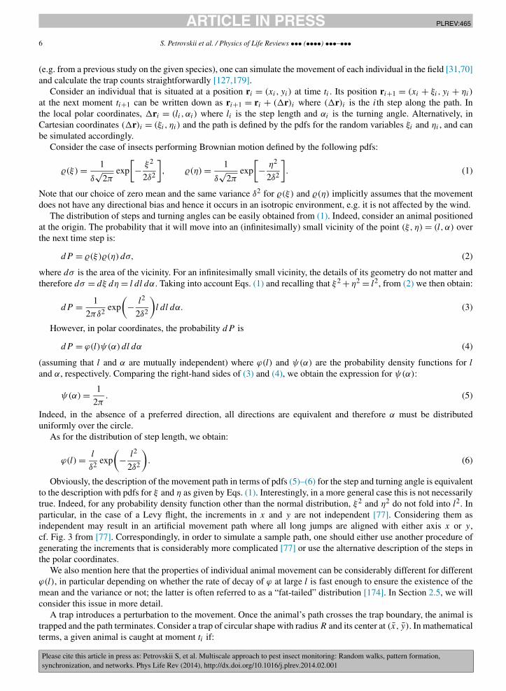
Fig. 2. Population of insects performing Brownian motion as defined by (1) with δ2 = 0.02; snapshots are shown at t = 0 (left) and t = 15 (right),i.e. after 1500 steps with a hypothetical value �t = 0.01. Only a part of the computational domain is shown, the total size is 100 × 100. The initialpopulation density is U0 = 1 which corresponds to the total initial population size of K = 104.
(xi − x)2 + (yi − y)2 < R2. (7)
In ecological applications, there is not just one insect wandering in the field but many of them, say, K . Corre-spondingly, when the population dynamics are simulated using the individual-based approach, at each time step thenew positions for all K animals are calculated using the same probability density functions.2 At each time step, afterthe new position for each of the insects has been simulated, the condition (7) is applied. The trap counts are obtainedaccordingly: when the position of an animal is first observed to be inside the trap, the corresponding path is terminatedand the trap count increases by one.
Fig. 2 shows snapshots of the population distribution simulated using the above procedure in a square arena ordomain L × L (with L = 100, in abstract units) and a circular trap of radius R = 5 installed in the center of thedomain. For the initial condition (Fig. 2, left), we first took K insects and distributed them randomly across the wholedomain, and then removed those whose position appeared to be inside the trap. This results in the average populationdensity of U0 = KL−2. Fig. 2 (right) shows the distribution obtained after 1500 steps, the probability density functionsof the random walk being given by the normal distributions (1) with variance δ2 = 0.02.
Note that this individual-based modeling procedure does not contain the time intervals explicitly. For a given pdf,the evolution of the population distribution in discrete time depends on the number of steps i but not on �t . However,here we recall that, in studies on individual animal movement, the time-discrete random walk is not inherent but isintroduced as a theoretical framework to describe time-continuous movement (e.g. see the beginning of this section).The time thus appears implicitly through the value of the variance: the larger the time interval �t between the twosubsequent fixations of the animal position, the larger is the variance of the step size distribution. Moreover, timebecomes explicit when the time-discrete random walk is linked to its time-continuous mean-field counterpart (seeSection 2.2). With this idea in mind, we can chose a certain value of �t ; in particular, for the simulation results shownin Fig. 2 we consider �t = 0.01.
In agreement with intuitive expectations, the trap introduces a spatially inhomogeneous perturbation into the popu-lation distribution. A visual inspection of Fig. 2 immediately reveals that the population density near the trap boundaryis smaller than the density far away from the trap. This is shown more explicitly in Fig. 3. Due to the finite populationsize, the density fluctuates stochastically around its average value U0 = 1. Considering the evolution of the populationdensity profile, we observe that the radius of the perturbed area grows with time; as will be further explained in thenext section, this transient behavior is a principle property of the system dynamics that determines the pattern in thetrap counts sequence over time.
It is readily seen that this emerging spatial pattern affects the trap counts. For any given level of insects movementactivity (i.e. for any given δ), the number of insects caught per unit time increases with the population density inthe vicinity of the trap. Therefore, on average (up to fluctuations of stochastic origin), the number of insects caught
2 Here we neglect the inter-individual interactions that can potentially lead to a variety of collective phenomena in movement and behavior,e.g. see [36,163].

JID:PLREV AID:465 /REV [m3SC+; v 1.188; Prn:4/03/2014; 13:24] P.8 (1-59)
8 S. Petrovskii et al. / Physics of Life Reviews ••• (••••) •••–•••
Fig. 3. Insect density as a function of the radial distance from the center of the trap corresponding to the snapshot shown in Fig. 2, right. The verticalline shows the position of the trap boundary.
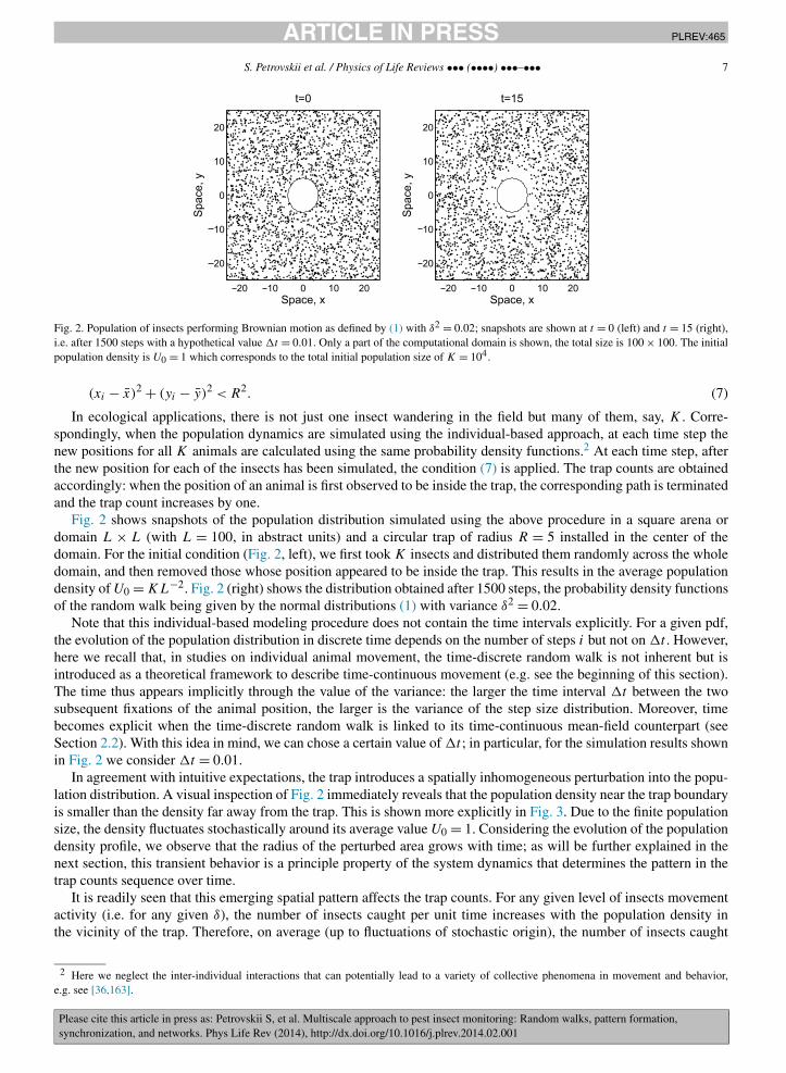
per unit time should gradually decrease with time. This heuristic argument appears to be in full agreement withsimulation results. Fig. 4 (top) shows the daily trap count C vs time over 3000 steps (100 steps = 1 day) obtained forinitial population density U0 = 0.1. The general tendency of daily counts to decrease with time can be readily seen,although the strong effect of stochasticity obscures the details of this pattern.
The pattern in the trap counts sequence is seen more clearly if, instead of daily counts, we consider a cumulativetrap count Jn defined as the sum of all daily counts up to the given day n:
Jn = J (tn) =n∑
i=1
Ci, (8)
where Ci is the trap count obtained in day i. The cumulative trap count obtained from the simulated daily countsshown in Fig. 4 (top) is shown in Fig. 4, bottom.
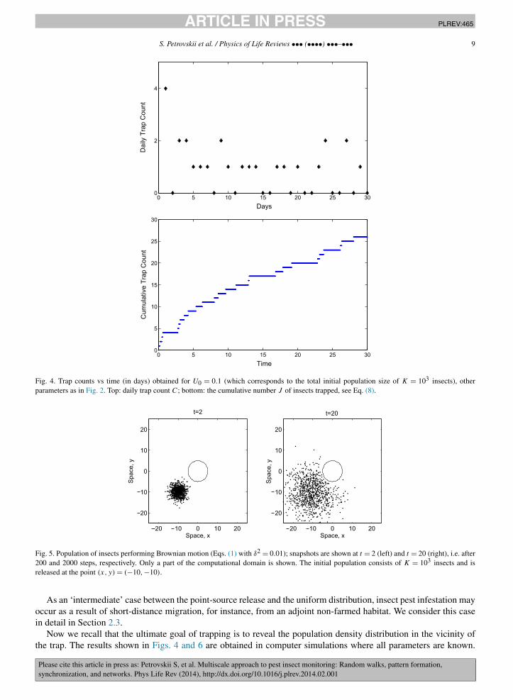
For a different initial distribution of the insects, both the emerging distribution and the pattern of trap counts canbe completely different. Fig. 5 shows the snapshots of the insect distribution at two moments of time obtained in thecase of a point-source release at the position x = −10, y = −10. Although the area occupied by the insects eventuallygrows in time, only very few insects reach the position of the trap boundary until approximately t = 5; see Fig. 6. Forany earlier time, the obtained trap counts are zero.
Note that, from the mathematical point of view, the choice of the initial conditions is likely to affect only theearly, transient stage of the dynamics before the system approaches some kind of ‘equilibrium state’. However, inapplications to pest monitoring and control, it is the transient stage – not the equilibrium state! – that is the focus ofinterest. Indeed, different initial population distributions correspond to different ecological situations that may requiredifferent control strategies. In particular, population aggregation (cf. Fig. 5) can arise for a variety of reasons such as apopulation response to environmental heterogeneity (when a favorable ‘patch’ has a much higher population densitythan the less favorable environment around it), self-organization due to spatiotemporal interspecific interactions [88],or swarming behavior [107]. The latter is especially important in the context of insect pest monitoring. Indeed, insectpest infestation often starts when an invasive or migrating swarm of pest insects lands in a small area inside anagricultural field. In this paper, we will refer to this situation as a ‘point-source release’. From this initial source, thepopulation then starts spreading over space. An early detection of the location of the population source, as well as theestimation of population size of the landed swarm, are therefore tasks of high practical importance for pest monitoringand control [58].
However, not all insect species migrate or disperse over long distances. Correspondingly, the uniform initialdistribution may arise naturally from the residual pest population (e.g. over-wintered or remaining after pesticidesapplication) dwelling in a relatively homogeneous environment.
JID:PLREV AID:465 /REV [m3SC+; v 1.188; Prn:4/03/2014; 13:24] P.9 (1-59)
S. Petrovskii et al. / Physics of Life Reviews ••• (••••) •••–••• 9
Fig. 4. Trap counts vs time (in days) obtained for U0 = 0.1 (which corresponds to the total initial population size of K = 103 insects), otherparameters as in Fig. 2. Top: daily trap count C; bottom: the cumulative number J of insects trapped, see Eq. (8).
Fig. 5. Population of insects performing Brownian motion (Eqs. (1) with δ2 = 0.01); snapshots are shown at t = 2 (left) and t = 20 (right), i.e. after200 and 2000 steps, respectively. Only a part of the computational domain is shown. The initial population consists of K = 103 insects and isreleased at the point (x, y) = (−10,−10).
As an ‘intermediate’ case between the point-source release and the uniform distribution, insect pest infestation mayoccur as a result of short-distance migration, for instance, from an adjoint non-farmed habitat. We consider this casein detail in Section 2.3.
Now we recall that the ultimate goal of trapping is to reveal the population density distribution in the vicinity ofthe trap. The results shown in Figs. 4 and 6 are obtained in computer simulations where all parameters are known.

JID:PLREV AID:465 /REV [m3SC+; v 1.188; Prn:4/03/2014; 13:24] P.10 (1-59)
10 S. Petrovskii et al. / Physics of Life Reviews ••• (••••) •••–•••
Fig. 6. Trap counts vs time (in days) obtained for a point-source release with parameters as in Fig. 5. Top: daily trap count C; bottom: the cumulativenumber J of insects trapped, see Eq. (8).
However, sequences of trap counts similar to Figs. 4 and 6 are routinely obtained in pest monitoring. How can weestimate the underlying population density or the location of point-source release, especially when the effects ofstochasticity are so strong that they make it almost impossible to distinguish any pattern in the counts sequences?In the next section, we will show that this can be done (often with surprisingly good accuracy, sometimes using adataset consisting of just several trap counts) by considering the stochastic trap counts together with their deterministicmean-field counterpart.
2.2. Mean-field approach: Diffusion equation
The individual-based approach considered in the previous section makes it possible to simulate the trap countsdirectly for any chosen initial distribution of insects and for any particular movement pattern as given by the prob-ability distributions of the step length and turning angle. This makes it possible to mimic various specific situationsin real-world pest control. However, a problem with the individual-based approach is that, since it is essentiallysimulation-based, it does not allow us to draw general conclusions about trap counts for different parameter values.
There is, however, another way to describe the trap counts. It is well known [17,33,34,107,160,168] that the pop-ulation density of a system of particles performing Brownian motion is a solution of the diffusion equation. Belowwe give a heuristic derivation of the diffusion equation; a rigorous derivation with a detailed discussion of all subtleissues arising on the way can be found, for instance, in [52,145].
Let us consider a single insect or ‘particle’ randomly browsing in an infinite space. For the sake of simplicity, herewe focus on the 1D case. Let G(x, t) be the probability density for this random walker to be found at the position x
at time t . Correspondingly, the probability to find the walker at time t in a small vicinity of x, i.e. in (x, x + dx), isPdx(x, t) = G(x, t) dx.

JID:PLREV AID:465 /REV [m3SC+; v 1.188; Prn:4/03/2014; 13:24] P.11 (1-59)
S. Petrovskii et al. / Physics of Life Reviews ••• (••••) •••–••• 11
The evolution of the probability density is described by the master equation [10,33,160]:
G(x, t + �t) =∞∫
−∞G(x − ξ, t)�(ξ,�t) dξ. (9)
In the context of the previous section, we consider Eq. (9) as a discrete-time model of an inherently continuousinsect movement, �t being the timescale of (discrete) observations. The kernel �(ξ,�t) is the probability density ofthe next position of the walker after time �t , i.e. after one step in time, if its position at time t is at the origin. Inecological studies, �(ξ,�t) defined as above is often called the dispersal kernel. Function � obviously depends on�t : increasing the time interval between the two subsequent fixations of the insect position, increases (on average) thecorresponding displacement. We consider the motion to be stationary (in the statistical sense) and to be taking placein a homogeneous space, so that � does not depend on x or t .
Eq. (9) is complemented by the initial condition:
G(x,0) = δ(x − x0), (10)
where x0 is the position of the walker at t = 0.Eq. (9) is very general and, as such, describes a variety of different stochastic processes. The type of the random
walk can be specified by assuming certain properties of the function �(ξ,�t). In particular, under certain constraints,the continuous-time limit �t → 0 of Eq. (9) turns into the Fokker–Planck equation, of which the diffusion equationis a special case.
With the continuous limit in mind, we consider �t to be sufficiently small and apply the Taylor expansion to theleft-hand side of (9) keeping explicitly only the first two terms, so that:
G(x, t + �t) = G(x, t) + ∂G(x, t)
∂t�t + o(�t), (11)
where the notation o(�t) is used to refer to all small terms of a higher order, so that o(�t)/�t → 0 when �t → 0.Since �(ξ,�t) is the probability density:
∞∫−∞
�(ξ,�t) dξ = 1, (12)
hence � must decay sufficiently fast at large ξ . Correspondingly, we assume that only small values of ξ contributesignificantly to the right-hand side of (9) and apply the Taylor expansion to G(x − ξ, t):
G(x − ξ, t) = G(x, t) − ∂G(x, t)
∂xξ + · · · + (−1)k
k!∂kG(x, t)
∂xkξk + · · · . (13)
An important property of � that distinguishes between different type of the random walk is its rate of decay atlarge ξ . In particular, if the rate of decay is exponential or faster, then, having substituted (11) and (13) into (9),Eq. (9) takes the following form:
∂G(x, t)
∂t�t + o(�t) =
∞∑k=1
(−1)k
k!∂kG(x, t)
∂xk
⟨ξk
⟩, (14)
where 〈ξk〉 is the kth moment of the probability distribution �:
⟨ξk
⟩ =∞∫
−∞ξk�(ξ) dξ < ∞, k = 1,2, . . . . (15)
We now restrict our analysis to the case where random movement is isotropic so that there is no directional bias.Correspondingly, �(ξ) = �(−ξ) and all odd moments disappear, 〈ξ2m+1〉 = 0 (m = 0,1, . . .). From (14), we thenobtain:

JID:PLREV AID:465 /REV [m3SC+; v 1.188; Prn:4/03/2014; 13:24] P.12 (1-59)
12 S. Petrovskii et al. / Physics of Life Reviews ••• (••••) •••–•••
∂G(x, t)
∂t+ o(�t)
�t=
∞∑m=1
(−1)k〈ξ2m〉k!�t
∂2mG(x, t)
∂x2m. (16)
Since � depends on �t , the moments depend on �t as well. Their dependence on the timescale differentiatesbetween different movement scenarios. Here we assume that the variance 〈ξ2〉 of the distribution � does not have asingularity at �t = 0 and that its Taylor expansion has a non-zero linear term:⟨
ξ2⟩ = 2D�t + o(�t), (17)
where the numerical coefficient 2D has the meaning of variance per unit time.A further standard assumption [10,52] is that, increasing the moment’s order increases the power of the first non-
zero term in the corresponding Taylor expansion, so that:⟨ξ2m
⟩ = o(�t) for m � 2. (18)
The random walk that satisfies conditions (15) and (17)–(18) is called Brownian motion.From (16)–(18), considering the limit �t → 0, we obtain the diffusion equation:
∂G(x, t)
∂t= D
∂2G(x, t)
∂x2, (19)
where D is the diffusion coefficient:
D = lim�t→0
〈ξ2〉2�t
.
Here the existence of the limit is guaranteed by (17).The solution of the diffusion equation corresponding to initial condition (10) is well known [37]:
G(x − x0, t) = 1√4πDt
exp
[− (x − x0)
2
4Dt
]. (20)
It is readily seen that the corresponding mean squared displacement of the walker is 〈(x − x0)2〉 ∼ Dt . This property
is widely regarded as a ‘fingerprint’ of the Brownian motion.Note that in the special case where the dispersal kernel is given by the normal distribution:
�(ξ,�t) = 1√4πD�t
exp
[− ξ2
4D�t
], (21)
the probability density for the single walker at t = n�t , i.e. after n steps, can be found from Eq. (9) by direct cal-culation. The mathematical fact that the convolution of two normal distributions is also a normal distribution is usedhere.
An important assumption made above is that � decays sufficiently fast at large ξ to ensure the existence of allmoments of the distribution, see (15). It is readily seen that this is true if �(ξ,�t) is the normal distribution. Fur-thermore, this holds for any kernel with the rate of decay exponential or faster. A question arises naturally as to howthe random walk properties may change if this constraint is relaxed and the kernel �(ξ,�t) is fat-tailed, so that someof the moments do not exist. An immediate example is given by the case where � decays as an inverse power law,i.e. � ∼ ξ−α for ξ → ∞ with α > 1. The corresponding pattern of movement is often referred to as “superdiffusion”[173] or, more broadly, as anomalous diffusion [81,174]. A detailed discussion of this phenomenon lies beyond thescope of this paper. Here we only very briefly mention some of its properties.
The situation appears to be different for α > 3 where the kernel possesses a finite variance and for 1 < α � 3where a finite variance does not exist. In the former case, the Central Limit Theorem applies [46], which predicts thatthe probability density G(x,n�t) of the walker after n steps (i.e. the sum of n independent identically distributedrandom values) converges to the normal distribution for n → ∞; see Fig. 7. Interestingly, the convergence occursnon-homogeneously in space, so that, for any finite n, the rate of decay at the tail of the probability distributionG(x,n�t) coincides with the rate of decay of the kernel [83], that is G ∼ (x − x0)
−α . Therefore, the tail of theevolving distribution remains fat. Thus, in spite of the normal distribution arising in the large-time limit, at any finite
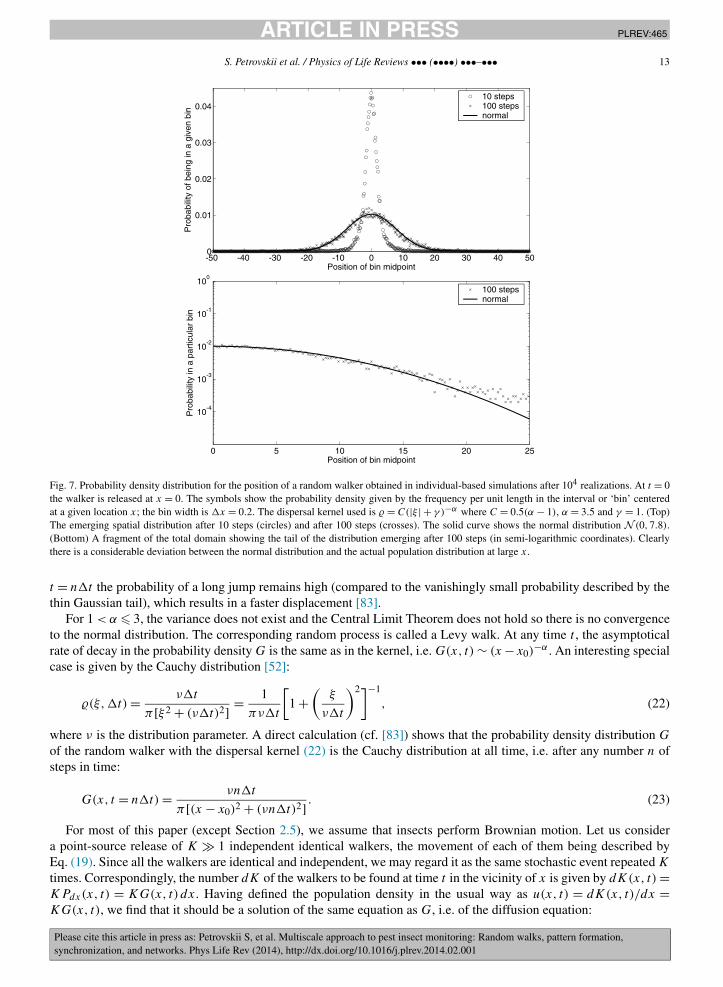
JID:PLREV AID:465 /REV [m3SC+; v 1.188; Prn:4/03/2014; 13:24] P.13 (1-59)
S. Petrovskii et al. / Physics of Life Reviews ••• (••••) •••–••• 13
Fig. 7. Probability density distribution for the position of a random walker obtained in individual-based simulations after 104 realizations. At t = 0the walker is released at x = 0. The symbols show the probability density given by the frequency per unit length in the interval or ‘bin’ centeredat a given location x; the bin width is �x = 0.2. The dispersal kernel used is � = C(|ξ | + γ )−α where C = 0.5(α − 1), α = 3.5 and γ = 1. (Top)The emerging spatial distribution after 10 steps (circles) and after 100 steps (crosses). The solid curve shows the normal distribution N (0,7.8).(Bottom) A fragment of the total domain showing the tail of the distribution emerging after 100 steps (in semi-logarithmic coordinates). Clearlythere is a considerable deviation between the normal distribution and the actual population distribution at large x.
t = n�t the probability of a long jump remains high (compared to the vanishingly small probability described by thethin Gaussian tail), which results in a faster displacement [83].
For 1 < α � 3, the variance does not exist and the Central Limit Theorem does not hold so there is no convergenceto the normal distribution. The corresponding random process is called a Levy walk. At any time t , the asymptoticalrate of decay in the probability density G is the same as in the kernel, i.e. G(x, t) ∼ (x −x0)
−α . An interesting specialcase is given by the Cauchy distribution [52]:
�(ξ,�t) = ν�t
π[ξ2 + (ν�t)2] = 1
πν�t
[1 +
(ξ
ν�t
)2]−1
, (22)
where ν is the distribution parameter. A direct calculation (cf. [83]) shows that the probability density distribution G
of the random walker with the dispersal kernel (22) is the Cauchy distribution at all time, i.e. after any number n ofsteps in time:
G(x, t = n�t) = νn�t
π[(x − x0)2 + (νn�t)2] . (23)
For most of this paper (except Section 2.5), we assume that insects perform Brownian motion. Let us considera point-source release of K 1 independent identical walkers, the movement of each of them being described byEq. (19). Since all the walkers are identical and independent, we may regard it as the same stochastic event repeated K
times. Correspondingly, the number dK of the walkers to be found at time t in the vicinity of x is given by dK(x, t) =KPdx(x, t) = KG(x, t) dx. Having defined the population density in the usual way as u(x, t) = dK(x, t)/dx =KG(x, t), we find that it should be a solution of the same equation as G, i.e. of the diffusion equation:
JID:PLREV AID:465 /REV [m3SC+; v 1.188; Prn:4/03/2014; 13:24] P.14 (1-59)
14 S. Petrovskii et al. / Physics of Life Reviews ••• (••••) •••–•••
∂u(x, t)
∂t= D
∂2u(x, t)
∂x2. (24)
The diffusion equation (19) for the probability density of a single walker is precise in the continuous limit �t → 0.However, one can expect that it remains valid, at least approximately, for a small but finite value of �t . In the corre-sponding approximate expression for the diffusion coefficient:
D ≈ δ2
2�t, (25)
δ2 is the variance of the probability density � of the next step’s length for the given value of �t . This is obviouslythe same δ2 that was used in the individual-based simulations in Section 2.1. Therefore, the diffusion coefficientlinks the “microscale” of an individual walker to the “macroscale” of the population density. We mention here thatthe diffusion equation for the population density could be derived in a completely different way based on Fick’s lawrelating population flux to the density gradient [17,37]. However, in that case the relationship between micro- andmacro-scales would remain obscure.
We mention here that, in mathematical terms, Eq. (19) (or (24)) should be classified as deterministic because it doesnot contain any random values. Although the random walk is a paradigm of stochastic dynamics, it is described bya purely deterministic diffusion equation. Therefore, the stochastic nature of the process does not necessarily requirean explicitly stochastic model. This observation is well known in physics3 but it is less commonly appreciated inbiological applications.
In fact, an explicitly stochastic model may only be required if we are interested in fluctuations, i.e. the devia-tions from the mean. In the particular case of Brownian motion, by virtue of the Central Limit Theorem the relativemagnitude of the fluctuations is:
�u
u∼ 1√
u.
Hence fluctuations are negligible for large population densities but may become important at small densities.In the case of a point-source release, the initial condition for Eq. (24) is given by u(x,0) = Kδ(x − x0) and the
spatial distribution of the population density is immediately obtained from (20) as u(x, t, x0) = KG(x − x0, t). In amore general case, u(x,0) = u0(x) where u0(x) is a certain function, it is straightforward to see (cf. [37]) that thesolution of the diffusion equation is
u(x, t) =∞∫
−∞G(x − ξ, t)u0(ξ) dξ. (26)
In practical applications concerned with trapping of walking or crawling insects, the diffusion equation should beconsidered on a 2D domain (on a 3D domain for flying insects). However, it is instructive to begin with a 1D casewhen the population density depends on one spatial coordinate only. Moreover, the traps used in pest monitoring oftenhave the shape of a long narrow slot ([21]; also [49]) and in that case 1D approximation can be expected to providenot only a qualitative but also a quantitative insight into the problem.
When the trap is installed, the movement space is not infinite anymore and the diffusion equation must be comple-mented with the boundary conditions. Let us consider a population of randomly walking insects in a field of size L. Forthe moment, we assume L is very large, DT L−2 � 1 where T is the characteristic trapping time. Correspondingly,we consider the diffusion equation in the semi-infinite domain 0 < x < ∞ (the effects of finiteness will be addressedlater) where the trap is installed at the left-hand side so that x = 0 corresponds to the trap boundary. Since there areno live insects in the trap, the relevant boundary condition is:
u(0, t) = 0. (27)
The corresponding solution of the diffusion equation is:
3 The Schrödinger equation would be another good example.

JID:PLREV AID:465 /REV [m3SC+; v 1.188; Prn:4/03/2014; 13:24] P.15 (1-59)
S. Petrovskii et al. / Physics of Life Reviews ••• (••••) •••–••• 15
Fig. 8. Population density vs space as given by the solution (33) of the diffusion equation (24) at t = 0.1 (solid curve 1), t = 1 (dashed-and-dottedcurve 2) and t = 10 (dashed curve 3) for parameters D = 1 and U0 = 10. From [127], with permissions.
u(x, t) =∞∫
0
[G(x − ξ, t) − G(x + ξ, t)
]u0(ξ) dξ (28)
(e.g. see [37]) where G is given by (20).Once the solution is known, the cumulative trap count over time t can be calculated as:
J (t) =t∫
0
∣∣j (τ )∣∣dτ, (29)
where:
j (t) = −D∂u(x, t)
∂x
∣∣∣∣x=0
(30)
is, according to Fick’s law, the diffusive flux of population density through the trap boundary.Considering (29)–(30) together with (28), after some standard calculations we obtain:
J (t) =∞∫
0
u0(ξ)
[1 − erf
(ξ√4Dt
)]dξ, (31)
where erf(z) is the error function.The properties of J as a function of time can therefore be different for different initial population distributions. In
the special but ecologically meaningful case of a homogeneous distribution u0(x) = U0 = const, from Eq. (31) wereadily obtain:
J (t) = 2U0√π
√Dt. (32)
The corresponding solution of the diffusion equation is given by:
u(x, t) = U0 erf
(x√4Dt
)(33)
and is shown in Fig. 8. Note that the size of the spatial perturbation induced by the trap grows with time as ∼ √Dt .
JID:PLREV AID:465 /REV [m3SC+; v 1.188; Prn:4/03/2014; 13:24] P.16 (1-59)
16 S. Petrovskii et al. / Physics of Life Reviews ••• (••••) •••–•••
Another relevant case is given by a distribution with constant gradient U1, i.e. u0(ξ) = U0 + U1ξ . This type ofinitial distribution may account for the migration of the pest species through the domain boundary; see Section 2.3. Inthis case, from (31) we obtain:
J (t) = 2U0√π
√Dt + U1Dt. (34)
A somewhat different case is given by the initial condition where the population is aggregated at a certain positionin space (‘point source release’, cf. Section 2.1), i.e. u0(x) = Kδ(x − x0) with K the total number of insects releasedat t = 0 at location x0 and δ is the Dirac function. In this case, Eq. (31) becomes:
J (t) = K
[1 − erf
(x0√4Dt
)]= K erfc
(x0√4Dt
). (35)
Recall that in the pest monitoring problem we are mostly interested in small time dynamics. Also, the position x0of the insects’ release is unlikely to be in close vicinity of the trap, so x0 can be regarded as large. Correspondingly, ofparticular interest is the limiting case where the argument z of erfc(z) is large. We can then make use of the followingasymptotic expansion [1]:
erfc(z) � 1√π
e−z2[
1
z+ o
(1
z
)]. (36)
Retaining only the leading term, from (35) and (36), we obtain:
J (t) � K√π
√4Dt
x0exp
(− x2
0
4Dt
). (37)
Eq. (37) gives the small-time dependence of the cumulative trap count in the case of a point-source release.Coming back to the main goal of the single-trap scale of pest monitoring, now we are going to consider how
Eqs. (31)–(35) can be used for the estimation of the population density or size of the monitored species. Indeed,predictions obtained from the diffusion equation result in smooth, continuous, deterministic curves while the trapcount data are given by a discrete/discontinuous set often wildly oscillating due to stochastic effects, e.g. see Fig. 4.In order to answer this question, we recall that, given that the individual insect movement can be regarded (at leaston a certain time scale) as a Brownian walk, the oscillations seen in the data occur around the value predicted by thediffusion equation. The unknown population density or total population size can be obtained by looking for the bestfit between theory and data [127]. This best fit can be found by using appropriate statistical tools.
The choice of the statistical tools is a controversial issue. The recent trend is to calculate the maximum likelihoodfunction and Akaike weights [29,56] as they are regarded as more reliable than other approaches. In this paper,however, in order to avoid unnecessary complexity, we use a simpler method of nonlinear regression [41] and theparameter estimation is done by using NLREG statistical software.4 Also, since our goal here is more to justify theconcept rather than to develop a ready-to-use practical toolkit, we restrict the analysis to a 1D case. Extension of theresults onto a more realistic 2D case is discussed at the end of this section.
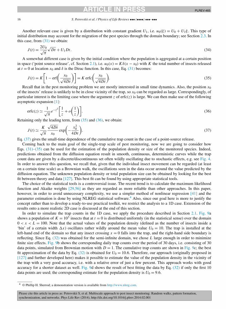
In order to simulate the trap counts in the 1D case, we apply the procedure described in Section 2.1. Fig. 9ashows a population of K = 103 insects that at t = 0 is distributed uniformly (in the statistical sense) over the domain0 < x < L = 100. Note that the actual values of the population density (defined as the number of insects inside a‘bin’ of a certain width �x) oscillates rather wildly around the mean value U0 = 10. The trap is installed at theleft-hand end of the domain so that any insect crossing x = 0 falls into the trap, and the right-hand side boundary isreflecting. Since Eq. (32) was obtained for the semi-infinite domain, we chose L large enough in order to minimizefinite size effects. Fig. 9b shows the corresponding daily trap counts over the period of 30 days, i.e. consisting of 30data points, simulated from Brownian motion with D = 1. The cumulative trap counts are shown in Fig. 9c; the bestfit approximation of the data by Eq. (32) is obtained for U0 = 10.6. Therefore, our approach (originally proposed in[127] and further developed here) makes it possible to estimate the value of the population density in the vicinity ofthe trap with a very good accuracy, i.e. with a relative error of just a few percent. This approach works with goodaccuracy for a shorter dataset as well. Fig. 9d shows the result of best fitting the data by Eq. (32) if only the first 10data points are used; the corresponding estimate for the population density is U0 = 9.6.
4 © Phillip H. Sherrod; a demonstration version is available from http://www.nlreg.com.
JID:PLREV AID:465 /REV [m3SC+; v 1.188; Prn:4/03/2014; 13:24] P.17 (1-59)
S. Petrovskii et al. / Physics of Life Reviews ••• (••••) •••–••• 17
Fig. 9. (a) The initial statistically-uniform distribution of the population of size K = 103: the circles show the number of insects per unit lengthafter they are binned with the width �x = 2, the dotted curve shows the mean value of the population density U0 = 10; (b) the daily trap counts;(c) the corresponding cumulative trap counts (shown by crosses) and their best-fit by the mean-field model (32) (shown by the solid curve), the bestfit is obtained for U0 = 10.6; (d) the results of data fitting in case of a smaller dataset, the best fit is obtained for U0 = 9.6.
Use of the more general formula (34) also allows the parameters (in this case, U0 and U1) to be obtained withreasonable accuracy. In particular, having applied it to the data shown in Fig. 9d (i.e. the trap counts after the first tendays), we find that the best fit is reached for U0 = 9.5 and U1 = 0.04 where the latter is not significantly differentfrom 0. In general, data fitting with a two-parameter formula is more demanding and, in order to reach a good accuracy,application of (34) may require a longer dataset compared to the one-parameter fit.
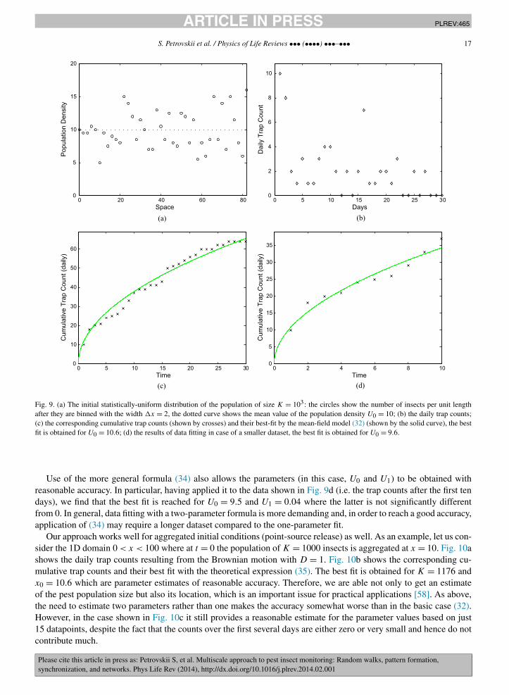
Our approach works well for aggregated initial conditions (point-source release) as well. As an example, let us con-sider the 1D domain 0 < x < 100 where at t = 0 the population of K = 1000 insects is aggregated at x = 10. Fig. 10ashows the daily trap counts resulting from the Brownian motion with D = 1. Fig. 10b shows the corresponding cu-mulative trap counts and their best fit with the theoretical expression (35). The best fit is obtained for K = 1176 andx0 = 10.6 which are parameter estimates of reasonable accuracy. Therefore, we are able not only to get an estimateof the pest population size but also its location, which is an important issue for practical applications [58]. As above,the need to estimate two parameters rather than one makes the accuracy somewhat worse than in the basic case (32).However, in the case shown in Fig. 10c it still provides a reasonable estimate for the parameter values based on just15 datapoints, despite the fact that the counts over the first several days are either zero or very small and hence do notcontribute much.

JID:PLREV AID:465 /REV [m3SC+; v 1.188; Prn:4/03/2014; 13:24] P.18 (1-59)
18 S. Petrovskii et al. / Physics of Life Reviews ••• (••••) •••–•••
Fig. 10. (a) The daily trap counts obtained for a point-source release of K = 1000 insects at a distance of x0 = 10 from the trap; (b) the correspondingcumulative trap counts (shown by crosses) and their best-fit by the mean-field model (35) (shown by the solid curve), the best fit is obtained forK = 1176 and x0 = 10.6; (d) the results of data fitting in case of a smaller dataset, the best fit is obtained for K = 848 and x0 = 9.8.
The domain used above was assumed to be large enough that the effect of the ‘external’ domain’s boundary at x = L
could be neglected. If this does not hold, one needs to define the boundary condition and consider the solution of thecorresponding boundary problem. Here we assume that there is no migration through the external field boundary:

JID:PLREV AID:465 /REV [m3SC+; v 1.188; Prn:4/03/2014; 13:24] P.19 (1-59)
S. Petrovskii et al. / Physics of Life Reviews ••• (••••) •••–••• 19
∂u(L, t)
∂x= 0. (38)
Applying the method of variable separation [37] to diffusion equation (24) with boundary conditions (27) and (38),we obtain the solution u in the form of an infinite series:
u(x, t) = 4U0
π
∞∑k=1
1
(2k − 1)sin
((2k − 1)πx
2L
)exp
(− (2k − 1)2π2Dt
4L2
). (39)
From (30) and (39), we arrive at the expression for the diffusion flux at the trap boundary:
j (t) = −D∂u(0, t)
∂x= −2DU0
L
∞∑k=1
exp
(− (2k − 1)2π2Dt
4L2
), (40)
so that the number of insects trapped over time t is then obtained using (29):
J (t) = 8LU0
π2
∞∑k=1
1
(2k − 1)2
[1 − exp
(− (2k − 1)2π2Dt
4L2
)], (41)
where LU0 is the total initial number of insects in the domain.Expression (41) is valid for any t . The more compact expressions obtained above for the semi-infinite domain
still apply, albeit approximately, if the observation time is not very large. In particular, in the case of a homogeneousinitial distribution, we find that the same formula (32) works with a good accuracy until the perturbation from the trapreaches the outside boundary, i.e. unless t becomes very large or else L is small [127].
The above results were obtained for a 1D system. A straightforward consideration of the diffusion equation inthe 2D case poses considerable technical difficulties; the corresponding solution is given by a series of the Besselfunctions where an explicit expression for the coefficients is not known. An extension of the 1D results onto the 2Dcase was done in [127] based on scaling and dimensions analysis and a relatively simple, semi-empirical formula forthe trap counts was obtained. The formula predicts that, in an infinitely large domain, the cumulative trap count J (t)
should become a linear function of time in the large-time limit. However, in a general case where the finiteness ofthe system cannot be neglected, J appears to be a linear combination of the small-time (∼ √
t ) and large-time (∼ t )asymptotics. The use of the formula to best-fit simulation data using nonlinear regression was shown to return anestimate of the corresponding population density with a reasonable accuracy of about 20% [127].
2.3. Boundary forcing
The goal of insect pest monitoring is to obtain information about pest abundance, in particular, with the purpose todetect signs of the pest population growth and hence to provide timely advice on pesticide application. An increasein the pest population size in a given agricultural field can occur because of the within-field population dynamicssuch as population multiplication due to reproduction. However, an increase in the pest density can also occur dueto migration of the species to the field from the outside areas. This leads to the questions of (i) how this effect ofpest immigration can affect the trap counts, (ii) whether it may be possible to distinguish between the effects of thenative and immigrating populations, and (iii) what is the relevant timescale of trap counts collection? Mathematically,immigration can be taken into account by imposing relevant conditions at the domain boundary, e.g. by defining thevalue of the in-flowing flux of the population density. Correspondingly, we will refer to the effect of pest immigrationas boundary forcing.
In Sections 2.1 and 2.2, pest immigration was taken into account indirectly by considering a point source release,i.e. the spatially aggregated initial population distribution. However, that only accounts for one possible ecologicalscenario where a swarm of insects arrives and lands at a certain location in the field. Another typical scenario occurswhen the given agricultural field adjoins a non-farmed area such as grassland or meadow. Non-farmed areas are rarelytreated against pests; as a result, such areas often become a refuge for pest species. The insects may then start spreadingfrom their refuge into the neighboring field(s).
Spreading can take place in different ways. If individual insects move around in a random manner, the migrationfrom the refuge to an adjoint farm-field goes against the population density gradient as described by Fick’s law.
JID:PLREV AID:465 /REV [m3SC+; v 1.188; Prn:4/03/2014; 13:24] P.20 (1-59)
20 S. Petrovskii et al. / Physics of Life Reviews ••• (••••) •••–•••
Alternatively, there can be a directed movement towards the farm-field, for instance due to the transport with thefavorable wind (for airborne species) or as a response to an odor emanating from the culture grown in the field.
We first consider the case where immigration occurs due to a directed movement. Transport through the fieldboundary is then described by the population flux jb = vUb where v is the velocity of the advection/migration and Ub
is the population density outside (i.e. in the non-farmed habitat). Assuming that inside the field the insects move in adiffusive manner, the corresponding boundary condition is:
−D∂u(r, t)
∂n
∣∣∣∣Λ
= (jb,n), (42)
where Λ is the field boundary and n is a unit normal vector pointing outside.In the analysis below, we focus on a 1D case where the field is described by the domain 0 < x < L. The trap is
installed at x = 0 and x = L is the external boundary where immigration occurs. Condition (42) then turns into thefollowing Neumann-type boundary condition at x = L:
∂u(L, t)
∂x= G, (43)
where G is the value of the density gradient. For the sake of simplicity, here we assume that both v and Ub areconstant, and hence G is constant as well.
Using the method of variable separation [37], it is relatively straightforward to obtain the solution of the diffusionequation with the boundary conditions (43) and (27) and to calculate the trap counts accordingly:
J (t)Neu = DGt + 16GL2
π3
∞∑k=1
(−1)k
(2k − 1)3
[1 − exp
(−D(2k − 1)2π2t
4L2
)]
+ 8U0L
π2
∞∑k=1
1
(2k − 1)2
[1 − exp
(−D(2k − 1)2π2t
4L2
)], (44)
where the product DG is the population density flux through the external boundary of the domain at x = L. In thespecial case of an impenetrable boundary, i.e. for G = 0, (44) coincides with (41).
Note that the first term in Eq. (44) corresponds to the large-time asymptotics. The linear increase of the trap countindicates the steady-state behavior. Indeed, it is readily seen that the large-time, steady-state limit of the diffusionequation,
d2us(x)
dx2= 0 where us(x) = lim
t→∞u(x, t), (45)
considered together with the boundary conditions (43) and (27), has the solution us(x) = Gx and hence the densitygradient dus/dx is constant and equal to G over the whole domain. The second and third terms in (44) thus describethe transient phase of the system. Here the third term describes the impact of the initial conditions (as it contains U0but not G) and the second term describes the transient boundary forcing (as it contains G but not U0).
Recall that, for t sufficiently small, the third term in (44) behaves like√
t (see the end of Section 2.2 and also[127] for more details) and hence is the leading term. Thus, the dynamics of the trap counts is a transition betweenthe two different asymptotics, i.e. between the small-time behavior J (t)Neu � √
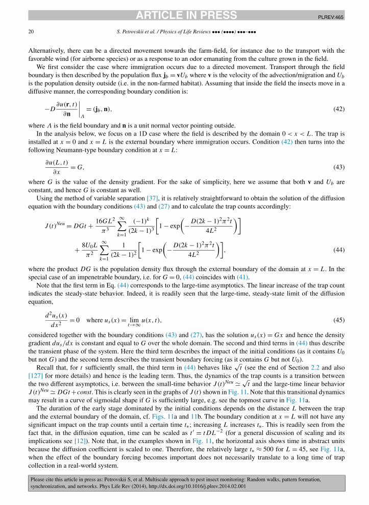
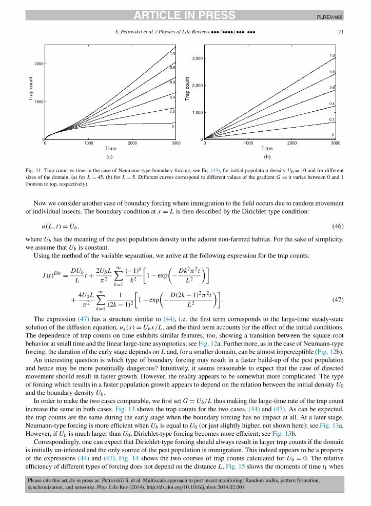
t and the large-time linear behaviorJ (t)Neu � DGt +const. This is clearly seen in the graphs of J (t) shown in Fig. 11. Note that this transitional dynamicsmay result in a curve of sigmoidal shape if G is sufficiently large, e.g. see the topmost curve in Fig. 11a.
The duration of the early stage dominated by the initial conditions depends on the distance L between the trapand the external boundary of the domain, cf. Figs. 11a and 11b. The boundary condition at x = L will not have anysignificant impact on the trap counts until a certain time t∗; increasing L increases t∗. This is readily seen from thefact that, in the diffusion equation, time can be scaled as t ′ = tDL−2 (for a general discussion of scaling and itsimplications see [12]). Note that, in the examples shown in Fig. 11, the horizontal axis shows time in abstract unitsbecause the diffusion coefficient is scaled to one. Therefore, the relatively large t∗ ≈ 500 for L = 45, see Fig. 11a,when the effect of the boundary forcing becomes important does not necessarily translate to a long time of trapcollection in a real-world system.
JID:PLREV AID:465 /REV [m3SC+; v 1.188; Prn:4/03/2014; 13:24] P.21 (1-59)
S. Petrovskii et al. / Physics of Life Reviews ••• (••••) •••–••• 21
Fig. 11. Trap count vs time in the case of Neumann-type boundary forcing, see Eq. (43), for initial population density U0 = 10 and for differentsizes of the domain, (a) for L = 45, (b) for L = 5. Different curves correspond to different values of the gradient G as it varies between 0 and 1(bottom to top, respectively).
Now we consider another case of boundary forcing where immigration to the field occurs due to random movementof individual insects. The boundary condition at x = L is then described by the Dirichlet-type condition:
u(L, t) = Ub, (46)
where Ub has the meaning of the pest population density in the adjoint non-farmed habitat. For the sake of simplicity,we assume that Ub is constant.
Using the method of the variable separation, we arrive at the following expression for the trap counts:
J (t)Dir = DUb
Lt + 2UbL
π2
∞∑k=1
(−1)k
k2
[1 − exp
(−Dk2π2t
L2
)]
+ 4U0L
π2
∞∑k=1
1
(2k − 1)2
[1 − exp
(−D(2k − 1)2π2t
L2
)]. (47)
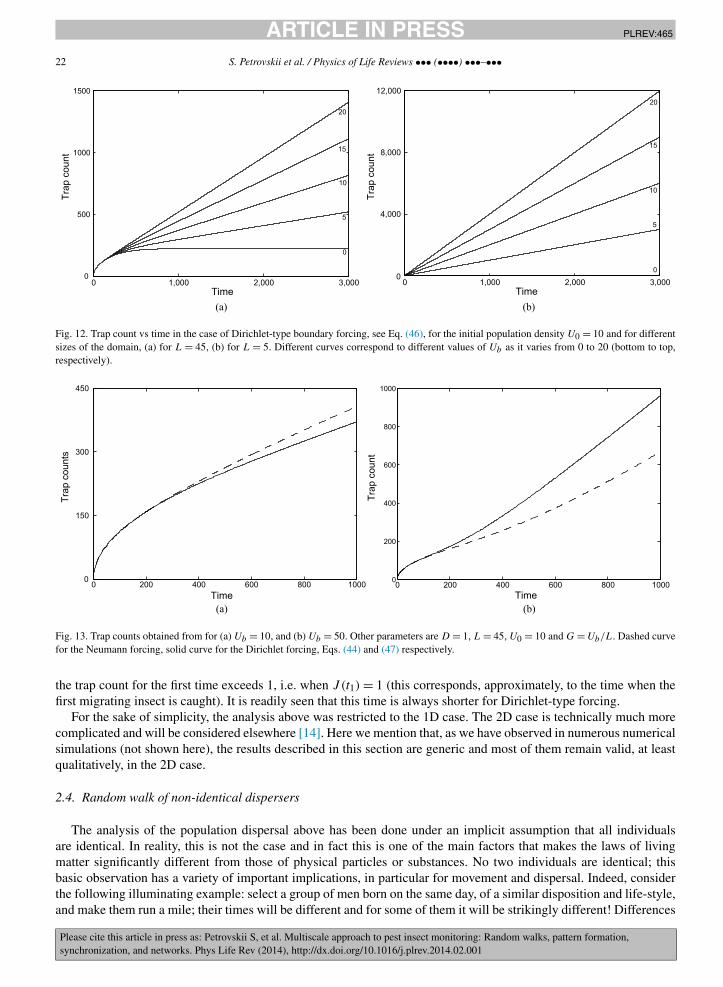
The expression (47) has a structure similar to (44), i.e. the first term corresponds to the large-time steady-statesolution of the diffusion equation, us(x) = Ubx/L, and the third term accounts for the effect of the initial conditions.The dependence of trap counts on time exhibits similar features, too, showing a transition between the square-rootbehavior at small time and the linear large-time asymptotics; see Fig. 12a. Furthermore, as in the case of Neumann-typeforcing, the duration of the early stage depends on L and, for a smaller domain, can be almost imperceptible (Fig. 12b).
An interesting question is which type of boundary forcing may result in a faster build-up of the pest populationand hence may be more potentially dangerous? Intuitively, it seems reasonable to expect that the case of directedmovement should result in faster growth. However, the reality appears to be somewhat more complicated. The typeof forcing which results in a faster population growth appears to depend on the relation between the initial density U0and the boundary density Ub .
In order to make the two cases comparable, we first set G = Ub/L thus making the large-time rate of the trap countincrease the same in both cases. Fig. 13 shows the trap counts for the two cases, (44) and (47). As can be expected,the trap counts are the same during the early stage when the boundary forcing has no impact at all. At a later stage,Neumann-type forcing is more efficient when Ub is equal to U0 (or just slightly higher, not shown here); see Fig. 13a.However, if Ub is much larger than U0, Dirichlet-type forcing becomes more efficient; see Fig. 13b.
Correspondingly, one can expect that Dirichlet-type forcing should always result in larger trap counts if the domainis initially un-infested and the only source of the pest population is immigration. This indeed appears to be a propertyof the expressions (44) and (47). Fig. 14 shows the two courses of trap counts calculated for U0 = 0. The relativeefficiency of different types of forcing does not depend on the distance L. Fig. 15 shows the moments of time t1 when
JID:PLREV AID:465 /REV [m3SC+; v 1.188; Prn:4/03/2014; 13:24] P.22 (1-59)
22 S. Petrovskii et al. / Physics of Life Reviews ••• (••••) •••–•••
Fig. 12. Trap count vs time in the case of Dirichlet-type boundary forcing, see Eq. (46), for the initial population density U0 = 10 and for differentsizes of the domain, (a) for L = 45, (b) for L = 5. Different curves correspond to different values of Ub as it varies from 0 to 20 (bottom to top,respectively).
Fig. 13. Trap counts obtained from for (a) Ub = 10, and (b) Ub = 50. Other parameters are D = 1, L = 45, U0 = 10 and G = Ub/L. Dashed curvefor the Neumann forcing, solid curve for the Dirichlet forcing, Eqs. (44) and (47) respectively.
the trap count for the first time exceeds 1, i.e. when J (t1) = 1 (this corresponds, approximately, to the time when thefirst migrating insect is caught). It is readily seen that this time is always shorter for Dirichlet-type forcing.
For the sake of simplicity, the analysis above was restricted to the 1D case. The 2D case is technically much morecomplicated and will be considered elsewhere [14]. Here we mention that, as we have observed in numerous numericalsimulations (not shown here), the results described in this section are generic and most of them remain valid, at leastqualitatively, in the 2D case.
2.4. Random walk of non-identical dispersers
The analysis of the population dispersal above has been done under an implicit assumption that all individualsare identical. In reality, this is not the case and in fact this is one of the main factors that makes the laws of livingmatter significantly different from those of physical particles or substances. No two individuals are identical; thisbasic observation has a variety of important implications, in particular for movement and dispersal. Indeed, considerthe following illuminating example: select a group of men born on the same day, of a similar disposition and life-style,and make them run a mile; their times will be different and for some of them it will be strikingly different! Differences
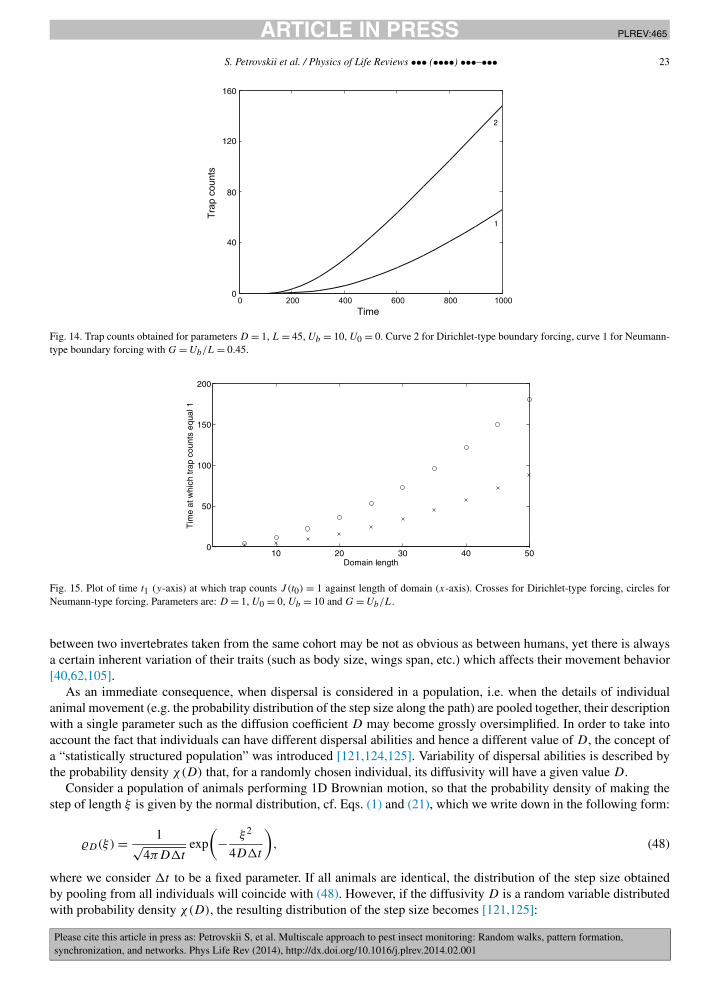
JID:PLREV AID:465 /REV [m3SC+; v 1.188; Prn:4/03/2014; 13:24] P.23 (1-59)
S. Petrovskii et al. / Physics of Life Reviews ••• (••••) •••–••• 23
Fig. 14. Trap counts obtained for parameters D = 1, L = 45, Ub = 10, U0 = 0. Curve 2 for Dirichlet-type boundary forcing, curve 1 for Neumann-type boundary forcing with G = Ub/L = 0.45.
Fig. 15. Plot of time t1 (y-axis) at which trap counts J (t0) = 1 against length of domain (x-axis). Crosses for Dirichlet-type forcing, circles forNeumann-type forcing. Parameters are: D = 1, U0 = 0, Ub = 10 and G = Ub/L.
between two invertebrates taken from the same cohort may be not as obvious as between humans, yet there is alwaysa certain inherent variation of their traits (such as body size, wings span, etc.) which affects their movement behavior[40,62,105].
As an immediate consequence, when dispersal is considered in a population, i.e. when the details of individualanimal movement (e.g. the probability distribution of the step size along the path) are pooled together, their descriptionwith a single parameter such as the diffusion coefficient D may become grossly oversimplified. In order to take intoaccount the fact that individuals can have different dispersal abilities and hence a different value of D, the concept ofa “statistically structured population” was introduced [121,124,125]. Variability of dispersal abilities is described bythe probability density χ(D) that, for a randomly chosen individual, its diffusivity will have a given value D.
Consider a population of animals performing 1D Brownian motion, so that the probability density of making thestep of length ξ is given by the normal distribution, cf. Eqs. (1) and (21), which we write down in the following form:
�D(ξ) = 1√4πD�t
exp
(− ξ2
4D�t
), (48)
where we consider �t to be a fixed parameter. If all animals are identical, the distribution of the step size obtainedby pooling from all individuals will coincide with (48). However, if the diffusivity D is a random variable distributedwith probability density χ(D), the resulting distribution of the step size becomes [121,125]:
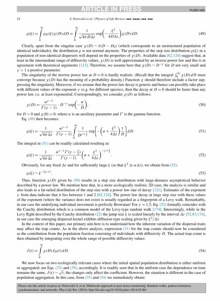
JID:PLREV AID:465 /REV [m3SC+; v 1.188; Prn:4/03/2014; 13:24] P.24 (1-59)
24 S. Petrovskii et al. / Physics of Life Reviews ••• (••••) •••–•••
�(ξ) =∞∫
0
�D(ξ)χ(D)dD =∞∫
0
1√4πD�t
exp
(− ξ2
4D�t
)χ(D)dD. (49)
Clearly, apart from the singular case χ(D) ∼ δ(D − D0) (which corresponds to an unstructured population ofidentical individuals), the distribution � is not normal anymore. The properties of the step size distribution �(ξ) in apopulation of non-identical dispersers will depend on the properties of χ(D). Available data [62,124] suggest that, atleast in the intermediate range of diffusivity values, χ(D) is well approximated by an inverse power law and this is inagreement with theoretical arguments [121]. Therefore, we assume here that χ(D) ∼ D−γ for D not very small andγ > 1 a positive parameter.
The singularity of the inverse power law at D = 0 is hardly realistic. (Recall that the integral∫ ∞
0 χ(D)dD mustconverge because χ(D) has the meaning of a probability density.) Function χ should therefore include a factor sup-pressing the singularity. Moreover, if we assume that the power law decay is generic and hence can possibly take placewith different values of the exponent γ (e.g. for different species), then the decay at D = 0 should be faster than anypower law, i.e. at least exponential. Correspondingly, we consider χ(D) as follows:
χ(D) = αγ−1
Γ (γ − 1)· D−γ exp
(− α
D
), (50)
for D > 0 and χ(0) = 0, where α is an auxiliary parameter and Γ is the gamma function.Eq. (49) then becomes:
�(ξ) = 1√4π�t
· αγ−1
Γ (γ − 1)
∞∫0
1
Dγ+ 12
exp
[−
(α + ξ2
4�t
)1
D
]dD. (51)
The integral in (51) can be readily calculated resulting in:
�(ξ) = 1√4π�t
· αγ−1Γ (γ − 12 )
Γ (γ − 1)
(α + ξ2
4�t
)−γ+ 12
. (52)
Obviously, for any fixed �t and for sufficiently large ξ (so that ξ2 α�t), we obtain from (52):
�(ξ) ∼ ξ−2γ+1. (53)
Thus, function χ(D) given by (50) results in a step size distribution with large-distance asymptotical behaviordescribed by a power law. We mention here that, in a more ecologically realistic 2D case, the analysis is similar andalso leads to a fat-tailed distribution of the step size with a power law rate of decay [121]. Estimates of the exponentγ from data indicate that it lies between 1 and 2 [62,124]. The power law decay at large step size with these valuesof the exponent (where the variance does not exist) is usually regarded as a fingerprint of a Levy walk. Remarkably,in our case the underlying individual movement is perfectly Brownian! For γ = 1.5, Eq. (52) formally coincides withthe Cauchy distribution which is a common model of the Levy-type random walk [174]. Interestingly, while in theLevy flight described by the Cauchy distribution (22) the jump size ξ is scaled linearly by the interval �t [52,83,174],in our case the emerging dispersal kernel exhibits diffusion-type scaling given by ξ2/�t .
In the context of this paper, our primary aim here is to understand how the inherent variation of the dispersal traitsmay affect the trap counts. As in the above analysis, expression (31) for the trap counts should now be consideredas the contribution from the population fraction consisting of individuals with diffusivity D. The actual trap count isthen obtained by integrating over the whole range of possible diffusivity values:
J (t) =∞∫
0
χ(D)JD(t) dD. (54)
We now focus on two ecologically relevant cases where the initial spatial population distribution is either uniformor aggregated; see Eqs. (32) and (35), accordingly. It is readily seen that in the uniform case the dependence on timeremains the same, J (t) ∼ √
t , the changes only affect the coefficient. However, the situation is different in the case ofpopulation aggregation. In this case, from (35) and (54) we immediately obtain:

JID:PLREV AID:465 /REV [m3SC+; v 1.188; Prn:4/03/2014; 13:24] P.25 (1-59)
S. Petrovskii et al. / Physics of Life Reviews ••• (••••) •••–••• 25
J (t) = K
∞∫0
χ(D) erfc
(x0√4Dt
)dD, (55)
where K is the initial population size. With χ(D) given by (50), Eq. (55) becomes:
J (t) = Kαγ−1
Γ (γ − 1)
∞∫0
D−γ exp
(− α
D
)erfc
(x0√4Dt
)dD. (56)
Having introduced a new variable as z = x0/√
4Dt , Eq. (56) takes the following form:
J (t) = 2Kαγ−1
Γ (γ − 1)·(
4t
x20
)γ−1 ∞∫0
z2γ−3 exp
(−4αt
x20
z2)
erfc(z) dz. (57)
Unfortunately, integral (57) can only be calculated analytically if 2γ − 3 = 1, i.e. for γ = 2. In this case, from (57)we obtain:
J (t) = K
[1 −
(1 + 4αt
x20
)− 12]. (58)
In the small-time limit (and/or for large x0), Eq. (58) becomes:
J (t) � 2αK
x20
t, (59)
which is completely different from the time dependence expected in the corresponding unstructured population,cf. Eq. (37).
2.5. Trapping of Levy-walking insects: time-dependent diffusion as an alternative framework?
In the previous sections, we presented a theory that allows the estimation of the parameters of a monitored popula-tion such as the population density in the vicinity of a trap (or the population size and the position of the point-sourcerelease) from trap counts. A presumption of our analysis is that the insects perform Brownian motion. Although thisis in many cases true [74,76,109,124], there has also been growing evidence that, under certain conditions, animalsof some species can follow a different movement pattern, such as Levy flight or walk5 [143,172,173]. An essentialdifference between the two patterns is that the relative frequency of long steps along the movement path is muchhigher in a Levy walk than in Brownian motion. Correspondingly, it can result in a faster dispersal, the phenomenonthat is known as “superdiffusion” [81,154].
In mathematical terms, a higher frequency of long steps means a lower rate of probability density decay at largedistances, a property often referred to as a ‘fat tail’ (in contrast to the ‘thin tail’ of the normal distribution). Note thathaving a probability density distribution with a fat tail is not by itself sufficient for having a Levy walk. Due to theCentral Limit Theorem [46], a sum of independent identical distributions, the first three moments of which are finite,converges to a normal distribution when the number of steps n tends to infinity (but preserving the power law decayat the distribution’s tail for any finite n, see Fig. 7 and also [83]). Therefore, in a 1D case, a genuine Levy walk onlyoccurs if the probability density �(ξ) of the step size ξ behaves at large ξ as � ∼ ξ−α with α � 3. Obviously such astochastic process is fat tailed and has no variance; random walks with this property are usually referred to as being‘scale-free’, although this terminology can be confusing [78].
Whether animals really perform Levy walk or not remains a highly controversial issue [16,167]. Some cases thatwere originally branded as evidence of Levy walk [172] were later re-classified as Brownian motion [43] and thenhave recently been re-classified as Levy walk again [142]. Standard statistical tools may sometimes fail to distinguishbetween power law and exponential rate of decay in the step size distribution [137]. The ‘observed’ movement type
5 Due to a long-standing confusion that has almost turned into a tradition, what is called a Levy walk in ecology often corresponds to what isknown as a Levy flight in physics [154].
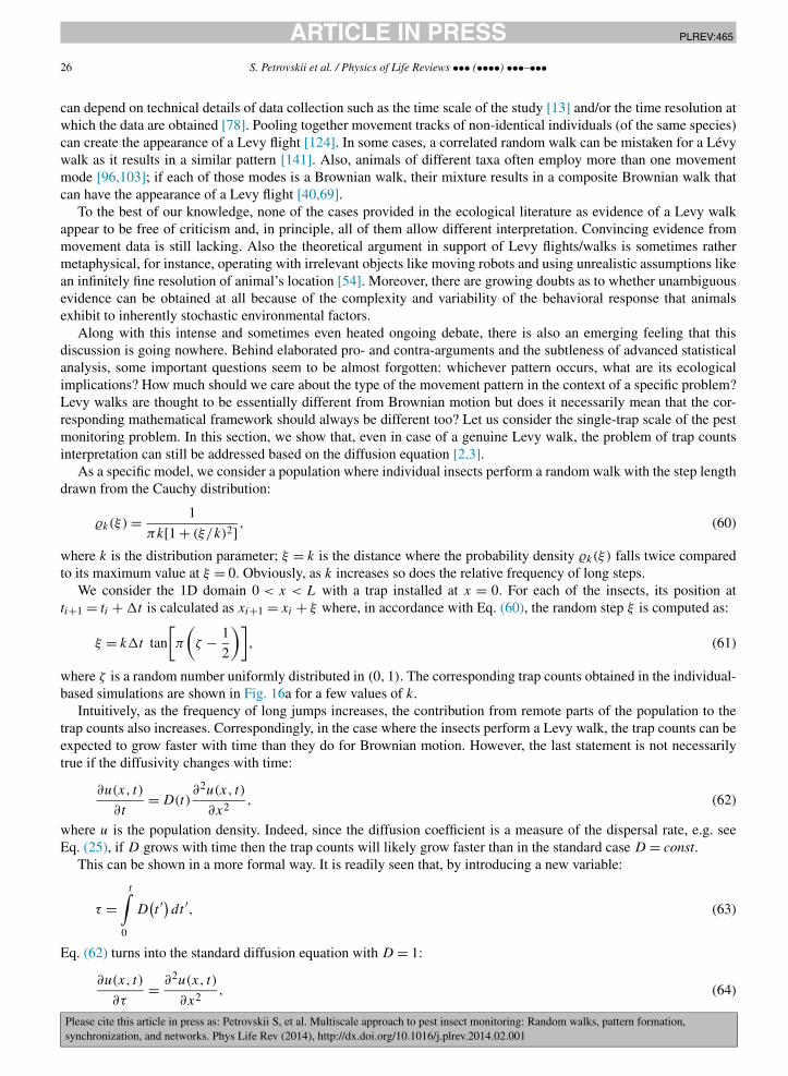
JID:PLREV AID:465 /REV [m3SC+; v 1.188; Prn:4/03/2014; 13:24] P.26 (1-59)
26 S. Petrovskii et al. / Physics of Life Reviews ••• (••••) •••–•••
can depend on technical details of data collection such as the time scale of the study [13] and/or the time resolution atwhich the data are obtained [78]. Pooling together movement tracks of non-identical individuals (of the same species)can create the appearance of a Levy flight [124]. In some cases, a correlated random walk can be mistaken for a Lévywalk as it results in a similar pattern [141]. Also, animals of different taxa often employ more than one movementmode [96,103]; if each of those modes is a Brownian walk, their mixture results in a composite Brownian walk thatcan have the appearance of a Levy flight [40,69].
To the best of our knowledge, none of the cases provided in the ecological literature as evidence of a Levy walkappear to be free of criticism and, in principle, all of them allow different interpretation. Convincing evidence frommovement data is still lacking. Also the theoretical argument in support of Levy flights/walks is sometimes rathermetaphysical, for instance, operating with irrelevant objects like moving robots and using unrealistic assumptions likean infinitely fine resolution of animal’s location [54]. Moreover, there are growing doubts as to whether unambiguousevidence can be obtained at all because of the complexity and variability of the behavioral response that animalsexhibit to inherently stochastic environmental factors.
Along with this intense and sometimes even heated ongoing debate, there is also an emerging feeling that thisdiscussion is going nowhere. Behind elaborated pro- and contra-arguments and the subtleness of advanced statisticalanalysis, some important questions seem to be almost forgotten: whichever pattern occurs, what are its ecologicalimplications? How much should we care about the type of the movement pattern in the context of a specific problem?Levy walks are thought to be essentially different from Brownian motion but does it necessarily mean that the cor-responding mathematical framework should always be different too? Let us consider the single-trap scale of the pestmonitoring problem. In this section, we show that, even in case of a genuine Levy walk, the problem of trap countsinterpretation can still be addressed based on the diffusion equation [2,3].
As a specific model, we consider a population where individual insects perform a random walk with the step lengthdrawn from the Cauchy distribution:
�k(ξ) = 1
πk[1 + (ξ/k)2] , (60)
where k is the distribution parameter; ξ = k is the distance where the probability density �k(ξ) falls twice comparedto its maximum value at ξ = 0. Obviously, as k increases so does the relative frequency of long steps.
We consider the 1D domain 0 < x < L with a trap installed at x = 0. For each of the insects, its position atti+1 = ti + �t is calculated as xi+1 = xi + ξ where, in accordance with Eq. (60), the random step ξ is computed as:
ξ = k�t tan
[π
(ζ − 1
2
)], (61)
where ζ is a random number uniformly distributed in (0,1). The corresponding trap counts obtained in the individual-based simulations are shown in Fig. 16a for a few values of k.
Intuitively, as the frequency of long jumps increases, the contribution from remote parts of the population to thetrap counts also increases. Correspondingly, in the case where the insects perform a Levy walk, the trap counts can beexpected to grow faster with time than they do for Brownian motion. However, the last statement is not necessarilytrue if the diffusivity changes with time:
∂u(x, t)
∂t= D(t)
∂2u(x, t)
∂x2, (62)
where u is the population density. Indeed, since the diffusion coefficient is a measure of the dispersal rate, e.g. seeEq. (25), if D grows with time then the trap counts will likely grow faster than in the standard case D = const.
This can be shown in a more formal way. It is readily seen that, by introducing a new variable:
τ =t∫
0
D(t ′)dt ′, (63)
Eq. (62) turns into the standard diffusion equation with D = 1:
∂u(x, t) = ∂2u(x, t)
2, (64)
∂τ ∂x
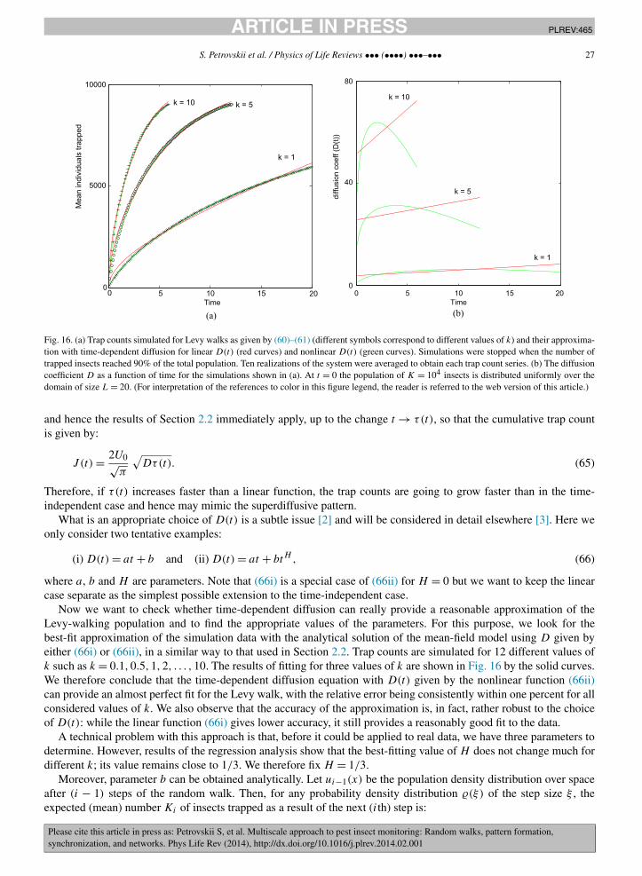
JID:PLREV AID:465 /REV [m3SC+; v 1.188; Prn:4/03/2014; 13:24] P.27 (1-59)
S. Petrovskii et al. / Physics of Life Reviews ••• (••••) •••–••• 27
Fig. 16. (a) Trap counts simulated for Levy walks as given by (60)–(61) (different symbols correspond to different values of k) and their approxima-tion with time-dependent diffusion for linear D(t) (red curves) and nonlinear D(t) (green curves). Simulations were stopped when the number oftrapped insects reached 90% of the total population. Ten realizations of the system were averaged to obtain each trap count series. (b) The diffusioncoefficient D as a function of time for the simulations shown in (a). At t = 0 the population of K = 104 insects is distributed uniformly over thedomain of size L = 20. (For interpretation of the references to color in this figure legend, the reader is referred to the web version of this article.)
and hence the results of Section 2.2 immediately apply, up to the change t → τ(t), so that the cumulative trap countis given by:
J (t) = 2U0√π
√Dτ(t). (65)
Therefore, if τ(t) increases faster than a linear function, the trap counts are going to grow faster than in the time-independent case and hence may mimic the superdiffusive pattern.
What is an appropriate choice of D(t) is a subtle issue [2] and will be considered in detail elsewhere [3]. Here weonly consider two tentative examples:
(i) D(t) = at + b and (ii) D(t) = at + btH , (66)
where a, b and H are parameters. Note that (66i) is a special case of (66ii) for H = 0 but we want to keep the linearcase separate as the simplest possible extension to the time-independent case.
Now we want to check whether time-dependent diffusion can really provide a reasonable approximation of theLevy-walking population and to find the appropriate values of the parameters. For this purpose, we look for thebest-fit approximation of the simulation data with the analytical solution of the mean-field model using D given byeither (66i) or (66ii), in a similar way to that used in Section 2.2. Trap counts are simulated for 12 different values ofk such as k = 0.1,0.5,1,2, . . . ,10. The results of fitting for three values of k are shown in Fig. 16 by the solid curves.We therefore conclude that the time-dependent diffusion equation with D(t) given by the nonlinear function (66ii)can provide an almost perfect fit for the Levy walk, with the relative error being consistently within one percent for allconsidered values of k. We also observe that the accuracy of the approximation is, in fact, rather robust to the choiceof D(t): while the linear function (66i) gives lower accuracy, it still provides a reasonably good fit to the data.
A technical problem with this approach is that, before it could be applied to real data, we have three parameters todetermine. However, results of the regression analysis show that the best-fitting value of H does not change much fordifferent k; its value remains close to 1/3. We therefore fix H = 1/3.
Moreover, parameter b can be obtained analytically. Let ui−1(x) be the population density distribution over spaceafter (i − 1) steps of the random walk. Then, for any probability density distribution �(ξ) of the step size ξ , theexpected (mean) number Ki of insects trapped as a result of the next (ith) step is:
JID:PLREV AID:465 /REV [m3SC+; v 1.188; Prn:4/03/2014; 13:24] P.28 (1-59)
28 S. Petrovskii et al. / Physics of Life Reviews ••• (••••) •••–•••
Fig. 17. Time dependent diffusion curves fitted to Levy walk trap counts, where H = 1/3, and b is determined from the first datapoint (at t = 0.1).Other parameters are the same as in Fig. 16a. Ten realizations of the system were averaged to obtain each trap count series.
Ki =L∫
0
dx · ui−1(x)
0∫−∞
dx′ �(x − x′). (67)
Since ui−1(x) is unknown, an explicit analytical expression for Ki for an arbitrary i does not seem possible toobtain. However, it is not difficult to find the number of insects caught after the first step because u0(x) is given by theinitial condition. Here we focus on the case u0(x) = U0 = const. Applying Eq. (67) to the Levy walk with the Cauchydistributed step size (60), we obtain:
K(L)1 =
(U0
πk
) L∫0
dx
0∫−∞
dx′
1 + ((x − x′)/k)2, (68)
where we add the superscript (L) in order to emphasize that (68) is obtained for the Levy walk. By calculating theintegral, (68) is simplified to:
K(L)1 = U0L
2− U0L
πarctan
(L
k
)+ U0k
2πlog
(1 + L2
k2
). (69)
On the other hand, the number of insects trapped after the first step can be obtained from the diffusion equation:
K(D)1 = 2U0√
π
[ �t∫0
D(t ′)dt ′
]1/2
= 2U0√π
[a
2(�t)2 + b
1 + H(�t)1+H
]1/2
, (70)
cf. Eq. (65), where we have assumed that L is not very small so that the effect of domain finiteness can still beneglected at time �t .
Setting K(L)1 = K
(D)1 , from (70) we obtain the expression for b:
b = π(1 + H)
4
(K
(L)1
U0L
)2
· L2
(�t)1+H− a(1 + H)
2· (�t)1−H . (71)
Here K(L)1 /(U0L) is the fraction of the total population trapped at the first step.
Correspondingly, the diffusion equation with D given by (66ii) has now only one parameter to be determined,i.e. a. Note that, with just one free parameter instead of three, the accuracy of the best-fitting approximation of theLevy walk data with time-dependent diffusion remains very good; see Fig. 17.
Therefore, we have a one-parameter solution of the diffusion equation which, for an appropriate choice of a,approximates very well the one-parameter stochastic model (60)–(61). We hypothesize that there is a relation betweena and k, i.e. a = a(k). Indeed, the existence of such relation seems obvious from Fig. 18a that shows the best-fittingvalues of a obtained for different k. Although we cannot calculate this relation analytically, the data shown in Fig. 18a
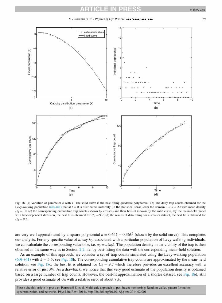
JID:PLREV AID:465 /REV [m3SC+; v 1.188; Prn:4/03/2014; 13:24] P.29 (1-59)
S. Petrovskii et al. / Physics of Life Reviews ••• (••••) •••–••• 29
Fig. 18. (a) Variation of parameter a with k. The solid curve is the best-fitting quadratic polynomial. (b) The daily trap counts obtained for theLevy-walking population (60)–(61) that at t = 0 is distributed uniformly (in the statistical sense) over the domain 0 < x < 20 with mean densityU0 = 10; (c) the corresponding cumulative trap counts (shown by crosses) and their best-fit (shown by the solid curve) by the mean-field modelwith time-dependent diffusion, the best fit is obtained for U0 = 9.7; (d) the results of data fitting for a smaller dataset, the best fit is obtained forU0 = 9.3.
are very well approximated by a square polynomial a = 0.64k − 0.36k2 (shown by the solid curve). This completesour analysis. For any specific value of k, say k0, associated with a particular population of Levy walking individuals,we can calculate the corresponding value of a, i.e. a0 = a(k0). The population density in the vicinity of the trap is thenobtained in the same way as in Section 2.2, i.e. by best-fitting the data with the corresponding mean-field solution.
As an example of this approach, we consider a set of trap counts simulated using the Levy-walking population(60)–(61) with k = 5.5; see Fig. 18b. The corresponding cumulative trap counts are approximated by the mean-fieldsolution, see Fig. 18c, the best fit is obtained for U0 = 9.7 which therefore provides an excellent accuracy with arelative error of just 3%. As a drawback, we notice that this very good estimate of the population density is obtainedbased on a large number of trap counts. However, the best-fit approximation of a shorter dataset, see Fig. 18d, stillprovides a good estimate of U0 with a relative error of about 7%.

JID:PLREV AID:465 /REV [m3SC+; v 1.188; Prn:4/03/2014; 13:24] P.30 (1-59)
30 S. Petrovskii et al. / Physics of Life Reviews ••• (••••) •••–•••
3. Single field problem: multiple traps
In the previous section, we showed how the population density of a pest insect can be evaluated based on thetrap counts obtained by a single trap. However, the information obtained in this way is local in the sense that it onlyreflects the pest abundance in a certain vicinity of the trap. Indeed, typical dispersal distances for walking insects areestimated to be on the order of 1 meter or less per day [171], which obviously corresponds to the diffusion coefficientD ∼ 1 m2 day−1. Assume that counts are collected daily. It was shown in Section 2.2 that ten trap counts are usuallyenough to obtain a population density estimate of good accuracy. Therefore, consider the total time T of trap exposureto be ten days. The mean squared displacement over this time is 〈x2〉 = 2DT ∼ 20 m2, thus giving the characteristicradius of the catchment area as 4.5 m. Agricultural fields rarely have area less than 1 ha, which gives a typical linearsize of around 100 m or more, whereas the spatial scale of variations in the population density distribution for walkinginsects is known to be 30–40 meters [47,65]. Therefore, an accurate monitoring may require more than one trap.
Correspondingly, we now consider the situation where the data are collected with several traps that are installed atcertain locations ri , i = 1, . . . ,N . That gives N values of the population density, u1, . . . , uN , where ui = u(ri ). Thequestion is how to estimate the average population density based on this information. The approach that is usuallyemployed in ecology suggests that it can be calculated by the arithmetic mean [38,159]:
m(N) = 1
N
N∑i=1
ui. (72)
An approximate value of the pest population size I can then be found by multiplying the sample mean by the area ofthe field A, that is:
I ≈ m(N)A. (73)
For convenience, below we will refer to (72)–(73) as the statistical rule.Reliability of the estimate (72) remains a disputable issue though [24,27]. One way to improve the accuracy is to
ensure that the size of the data set is large enough, i.e. that enough traps are installed. In theory, the sample mean valuegiven by Eq. (72) is known to converge to the exact value of the population size when N tends to infinity (cf. [46]).Hence we can expect better accuracy of the estimate when N gets larger. In practice, however, there is a trade-offbetween the number of traps needed to achieve sufficient accuracy and the number that can be afforded. If trappingis used in ecological research, the number N of traps per given area can be made quite large, e.g. on the order ofhundreds. Meanwhile, in routine pest monitoring programs N rarely exceeds twenty [91] and, in some cases, it can beas small as just one or a few traps per field [104]. There are several reasons why the number of traps cannot be madelarge. An increase in the number of traps or samples equates to an increase in the amount of labour and hence financesrequired. In any real-world situation, such resources are limited. Besides, traps introduce a disturbance into the fieldand installing a large number of them can damage the corresponding agricultural product.
Another problem with Eq. (72) is that it is spatially implicit, i.e. it takes into account neither the spacing betweenthe traps (which, generally speaking, can be variable) nor any information about the properties of the populationspatial distribution. Clearly, a spatially-explicit generalization of (72) is likely to provide, for the same number oftraps, a better quality estimate of the average population density.
The essence of the problem can be seen from Fig. 19. For the sake of simplicity, we show it in a hypothetical1D domain. Five traps are installed over the field. However, their location misses the high-density peak betweenthe second and third traps. As a result, the estimate obtained with (72) is going to underestimate the actual averagedensity considerably. The questions therefore arise as to (i) whether the existence of the peak could possibly be betteraccounted for if a more advanced approach is used instead of Eq. (72) and (ii) how the number of the traps and/ortheir location can be optimized with respect to the population spatial distribution. These two issues will be the mainfocus of this section.
Interestingly, the problem of evaluation of the average population density based on local density values, if addressedformally, almost coincides with the problem of numerical integration. One important difference is that, for the reasonsmentioned above, the number of the grid nodes (i.e. traps) cannot be made large as is usually assumed in the numericalintegration theory. This brings to the fore the challenging problem of integration on coarse grids. In recent years,intensive study of numerical integration methods for ecological applications has been carried out [44,45,114–116,118,119] and here we briefly summarize our experience and highlight the main results obtained.

JID:PLREV AID:465 /REV [m3SC+; v 1.188; Prn:4/03/2014; 13:24] P.31 (1-59)
S. Petrovskii et al. / Physics of Life Reviews ••• (••••) •••–••• 31
Fig. 19. A sketch of data collection with multiple traps. The diamonds gives the value of the density at the location of the traps X1, . . . ,X5 whilstthe dashed curve shows the actual population distribution.
3.1. Evaluation of pest insect abundance from discrete data
In this section, we briefly revisit the basics of numerical integration. Consider the domain Ω where the pest insectmonitoring is carried out (e.g. a farm-field). Let N be the total number of traps installed across the field Ω . Let usassume that we have already reconstructed the pest population density ui ≡ u(ri ) at the trap locations ri , i = 1, . . . ,N
(e.g. using the approaches described in Section 2). Hence our next goal is to evaluate pest abundance I from the pestpopulation density values ui ≡ u(ri ).
If we had a continuous pest population density function u(r) defined at any point r = (x, y) of the domain Ω , thenthe pest abundance I in the field would, by the definition of density, be given by the following integral:
I =∫ ∫
Ω
u(r) dr. (74)
However, the pest population density is only available to us at a discrete set of points ri , i = 1, . . . ,N . Conse-quently the above integral cannot be evaluated exactly and is instead approximated by means of numerical integration.A generic numerical integration formula is given by (e.g. see [39]):
I ≈ Ia(N) =N∑
i=1
ωiui, (75)
where Ia(N) is an approximation of the exact integral I , and ωi , i = 1, . . . ,N , are weight coefficients that definea particular method of integration. Correspondingly, in the context of numerical integration, the set of points {ri} iscalled the numerical grid.
For any chosen method of numerical integration and any fixed number of traps N used to collect the data, theaccuracy of an approximation Ia(N) is assessed by analyzing the integration error. Let us assume that the exact valueI of the pest abundance (74) is known to us. The relative integration error e(N) is defined as:
e(N) = |I − Ia(N)|I
. (76)
The integration error e(N) (also known as the approximation error) emerges because we replace a continuousfunction u(r) with a discrete function ui , i = 1, . . . ,N . The less data we use in the approximation (75), the bigger theintegration error we should expect. The aim of pest monitoring is to obtain a reliable estimate of the pest abundance;therefore, large values of the approximation error are unacceptable. The largest acceptable value of the error e is calledthe tolerance τ of the estimate. In other words, the relative error (76) should satisfy the following condition:
e(N)� τ, (77)
where τ is a specified tolerance. In ecological applications, the tolerance of τ ∼ 0.2–0.5 is usually considered asacceptable accuracy [111,152].
The integration error (76) depends on the number of the grid nodes N (i.e. the number of traps) but it also dependson the definition of weight coefficients in the formula (75). For a given N , different methods of numerical integration
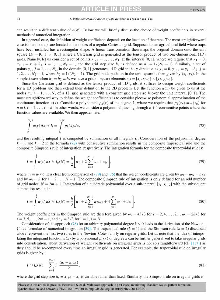
JID:PLREV AID:465 /REV [m3SC+; v 1.188; Prn:4/03/2014; 13:24] P.32 (1-59)
32 S. Petrovskii et al. / Physics of Life Reviews ••• (••••) •••–•••
can result in a different value of e(N). Below we will briefly discuss the choice of weight coefficients in severalmethods of numerical integration.
In a general case, the definition of weight coefficients depends on the location of the traps. The most straightforwardcase is that the traps are located at the nodes of a regular Cartesian grid. Suppose that an agricultural field where trapshave been installed has a rectangular shape. A linear transformation then maps the original domain onto the unitsquare Ω1 = [0,1] × [0,1] where a Cartesian grid is generated as the tensor product of two one-dimensional (1D)grids. Namely, let us consider a set of points xi , i = 1, . . . ,N1, at the interval [0,1], where we require that x1 = 0,xi+1 = xi + h1, i = 1, . . . ,N1 − 1, and the grid step size h1 is defined as h1 = 1/(N1 − 1). Similarly, a set ofpoints yj , j = 1, . . . ,N2, in the domain [0,1] generates a 1D grid in the y-direction as y1 = 0, yj+1 = yj + h2, j =1,2, . . . ,N2 − 1, where h2 = 1/(N2 − 1). The grid node position in the unit square is then given by (xi, yj ). In thesimplest case when h1 = h2 ≡ h, we have a grid of square elements cij = [xi, xi+1] × [yj , yj+1].
Since the Cartesian grid is defined as the tensor product of 1D grids, it suffices to design weight coefficientsfor a 1D problem and then extend their definition to the 2D problem. Let the function u(x) be given to us at thenodes xi , i = 1, . . . ,N , of a 1D grid generated with a constant grid step size h over the unit interval [0,1]. Themost straightforward way to define the weight coefficients is to consider piecewise polynomial approximation of thecontinuous function u(x). Consider a polynomial pk(x) of the degree k, where we require that pk(xn) = u(xn) forn = i, i + 1, . . . , i + k. In other words, we consider a polynomial passing through k + 1 consecutive points where thefunction values are available. We then approximate:
xi+k∫xi
u(x) dx ≈ Ii =xi+k∫xi
pk(x) dx, (78)
and the resulting integral I is computed by summation of all integrals Ii . Consideration of the polynomial degreek = 1 and k = 2 in the formula (78) with consecutive summation results in the composite trapezoidal rule and thecomposite Simpson’s rule of integration, respectively. The integration formula for the composite trapezoidal rule is:
I =1∫
0
u(x)dx ≈ Ia(N) = h
2
[u1 + 2
N−1∑i=2
ui + uN
], (79)
where ui ≡ u(xi). It is clear from comparison of (79) and (75) that the weight coefficients are given by ω1 = ωN = h/2and by ωi = h for i = 2, . . . ,N − 1. The composite Simpson rule of integration is only defined for an odd numberof grid nodes, N = 2m + 1. Integration of a quadratic polynomial over a sub-interval [xi, xi+2] with the subsequentsummation results in:
I =1∫
0
u(x)dx ≈ Ia(N) = h
3
[u1 + 2
m−1∑i=1
u2i+1 + 4m∑
i=1
u2i + uN
]. (80)
The weight coefficients in the Simpson rule are therefore given by ωi = 4h/3 for i = 2,4, . . . ,2m, ωi = 2h/3 fori = 3,5, . . . ,2m − 1, and ωi = h/3 for i = 1, i = N .
Consideration of the approach (78) for an arbitrary polynomial degree k > 0 leads to the derivation of the Newton–Cotes formulae of numerical integration [39]. The trapezoidal rule (k = 1) and the Simpson rule (k = 2) discussedabove represent the first two rules in the Newton–Cotes family on regular grids. Let us note that the idea of interpo-lating the integrand function u(x) by a polynomial pk(x) of degree k can be further generalized to take irregular gridsinto consideration, albeit derivation of weight coefficients on irregular grids is not so straightforward (cf. [117]) asthey should be re-computed every time an irregular grid is generated. For example, the trapezoidal rule on irregulargrids is given by:
I ≈ Ia(N) =N−1∑i=1
hi
(ui + ui+1)
2, (81)
where the grid step size hi = xi+1 − xi is variable rather than fixed. Similarly, the Simpson rule on irregular grids is:
JID:PLREV AID:465 /REV [m3SC+; v 1.188; Prn:4/03/2014; 13:24] P.33 (1-59)
S. Petrovskii et al. / Physics of Life Reviews ••• (••••) •••–••• 33
I ≈ Ia(N) =N−1
2∑i=1
h2i−1 + h2i
6(u2i−1 + 4u2i + u2i+1), (82)
which also relies on the variable grid step size hi = xi+1 −xi . As with the conventional Simpson rule (80), the numberof grid nodes N is required to be odd.
Once the integration techniques have been designed in the 1D case, they can be extended to the two-dimensional(2D) case. Namely:
I =1∫
0
1∫0
u(x, y) dx dy =∑i,j
Iij , (83)
where:
Iij =xi+1∫xi
yj+1∫yj
u(x, y) dx dy. (84)
Hence, the integration problem is reduced to the evaluation of the integral in each sub-domain cij = [xi, xi+1] ×[yj , yj+1] of the Cartesian grid. Integration on rectangular elements cij can, in turn, be further reduced to consecutiveapplication of the 1D formulae. Consider, for example, the simplest case of a regular grid with a constant grid stepsize h in both directions x and y. The integration technique is as follows. First, the integral (84) is re-written as:
Iij =yj+1∫yj
U(y)dy, (85)
where U(y) = ∫ xi+1xi
u(x, y) dx. We then employ 1D Newton–Cotes formulae in order to evaluate the function U(y)
in the square cell cij . Once the values of U(y) have been computed, the same integration rule can be applied toapproximate the 1D integral (85). For example, the trapezoidal rule of integration implies the approximation of u(x, y)
by a linear function on each sub-domain cij . Correspondingly, the integral Iij is evaluated as:
Iij ≈ h2
4[uij + ui+1,j + ui,j+1 + ui+1,j+1], (86)
where uij ≡ u(xi, yj ). The application of the Simpson rule in the cell cij requires that the data u(x, y) are availableat points (xi+q, yj+r ), where q = 0,1,2 and r = 0,1,2. The function u(x, y) is then integrated in the cell cij as:
Iij ≈ h2
36
[uij + ui,j+2 + ui+2,j + ui+2,j+2
+ 4(ui,j+1 + ui+1,j + ui+2,j+1 + ui+1,j+2) + 16ui+1,j+1]. (87)
Note that, like in the 1D case, integration by the Simpson rule requires an odd number of nodes N in each direction x
and y of the 2D regular grid.For irregular grids, numerical integration in the 2D case can be significantly more difficult compared to 1D integra-
tion. If the irregular grid is of Cartesian type (with a variable grid step size in each direction) then an approach similarto the one described above for regular grids (cf. Eq. (85)) can still be applied. However, the situation becomes muchmore complicated when the traps are located arbitrarily so that the grid of traps cannot be mapped onto a regularCartesian grid in the unit square. In scientific computing, such ‘truly irregular’ grids are called unstructured grids.An unstructured grid normally appears in a 2D problem as a set of non-overlapping triangles that covers the entiredomain [32]. There are two situations when such grids may be needed. First, the domain can in some cases have asophisticated geometry so that installation of traps at nodes of a Cartesian grid may not well resolve a curvilinearboundary of the domain. Second, an irregular grid may be required in order to avoid a bias in the trap counts [5,91]if there is a reason to believe that such a bias can significantly affect the data, e.g. when the environment has its ownregular structure as would an orchard or plantation.

JID:PLREV AID:465 /REV [m3SC+; v 1.188; Prn:4/03/2014; 13:24] P.34 (1-59)
34 S. Petrovskii et al. / Physics of Life Reviews ••• (••••) •••–•••
On an unstructured 2D grid, Eq. (85) obviously does not apply and a different approach should be used. After thetriangulation of the domain, the vertices of each triangle are considered as grid nodes where the function u(x, y) isdefined (i.e. where the traps are installed). One can then use local polynomial reconstruction of the integrand u(x, y)
by a least-squares method and integrate the resulting polynomial in each triangle. The least-squares technique forpolynomial reconstruction of the integrand function has been discussed in our previous work [119].
Numerical integration on an unstructured grid is, in principle, an efficient technique to evaluate the populationsize from discrete data collected with any random spatial distribution of traps. However, to the best of our knowledgeirregular grids remain relatively rare in ecological applications, even when used or considered in a broader context [64,67,166,177]. One problem with the use of unstructured grids, in particular in the pest abundance evaluation problem,is that the accuracy of polynomial reconstruction on such grids can depend heavily on the grid geometry [112,113].The issue of accuracy of numerical integration on unstructured grids therefore requires further careful investigationbefore they can be employed for numerical integration of the pest population density. For these reasons, in this paperwe mostly focus on the application of regular grids.
Our discussion in this section has mostly been concerned with the definition of the weight coefficients based onthe idea that the integrand function u(x, y) is replaced with a polynomial. It is worth mentioning here that there existsa big class of alternative methods of numerical integration, Gauss quadrature being perhaps the most well-known ofthem [39]. However, we are not aware of any cases where those methods have been applied to ecological problemsand hence we do not discuss them in this paper.
3.2. Evaluation of population abundance on coarse grids
Application of numerical integration methods to the problem of insect pest abundance evaluation was first consid-ered in [116] and then further developed in [44,114,115,118,119]. Examples of numerical integration of either fielddata or ecologically meaningful simulation data can be found in [115–117,119] where a detailed discussion of thenumerical procedure and the related issues has been provided. Several methods of numerical integration have beenconsidered. In particular, the trapezoidal rule and the Simpson rule of integration have been discussed thoroughly bothin the 1D and 2D cases. Also, methods based on reconstruction of the integrand function by higher order polynomialswere studied in [116,117] for a 1D problem and were briefly discussed in [119] in the 2D case. Given the variety ofavailable numerical integration techniques, questions arise with regard to their relative accuracy and efficiency: aresome methods better than others and, if yes, what is a criterion for the selection of the best one?
The standard theory of numerical integration is based on the concept of convergence rate. The key requirement ofany method of numerical integration is that weight coefficients should satisfy the following condition:
Ia(N) → I for N → ∞, (88)
where N is the number of the grid nodes. The design of weight coefficients in any method of numerical integrationis based on this condition. Meanwhile, apart from the convergence as such, it is also important to understand howfast the approximate value Ia(N) actually approaches the exact value of the integral I when N increases. Differentmethods of numerical integration can have different convergence rates.
In order to illustrate the concept, let us consider a 1D problem on a regular grid. The idea of convergence rate canbe broadly described by the following relation:
e(N) � Chp = O(hp
), (89)
where h is the distance between grid nodes, and the coefficient C and the exponent p depend on the method ofnumerical integration used in the problem. In particular, p is fully determined by the choice of weight coefficients. Ona regular Cartesian grid h = 1/(N − 1) and Eq. (88) can be re-written in terms of the grid step size h as Ia(h) → I forh → 0. Eq. (89) described how the integration error e(h) tends to zero for a particular method of numerical integration,and in particular the speed of this process. We emphasize here that the theory of numerical integration normally dealswith asymptotic convergence so that, strictly speaking, Eqs. (88)–(89) are only valid when h is sufficiently small.
The theory states [39] that the statistical rule (72)–(73) has convergence rate O(h) while the convergence of thecomposite Simpson rule (80) is O(h4); see Fig. 20. This means that doubling the number of grid nodes will decreasethe error of the Simpson method by a factor of 16, while the error of the statistical rule is only halved. Therefore,a much bigger number of grid nodes (i.e. much larger number of traps) is required to achieve the same accuracy τ
JID:PLREV AID:465 /REV [m3SC+; v 1.188; Prn:4/03/2014; 13:24] P.35 (1-59)
S. Petrovskii et al. / Physics of Life Reviews ••• (••••) •••–••• 35
Fig. 20. Comparison of convergence rates. The relative integration error (76) is calculated as a function of the number of the grid nodes N in aregular grid with h = 1/(N − 1). The open circles (dashed line) and the closed squares (solid line) show the error (on the logarithmic scale) for thestatistical rule (72)–(73) and the Simpson rule (80), respectively.
(cf. Eq. (77)) if the statistical rule is employed in the evaluation of insect abundance compared to the Simpson rule. Inother words, for the same number of grid nodes, the Simpson rule will give a much better accuracy.
The above consideration clearly leads to the conclusion that, when choosing from available methods of numericalintegration with which to evaluate the total pest population size, the method with the fastest convergence rate (89) mustbe employed and other methods should simply be ignored. If we approximate the integrand function by a polynomial,the convergence rate will depend on the polynomial degree, higher order polynomial approximation having fasterconvergence [39]. For example, the 1D composite Simpson method with the convergence O(h4) should always bemore accurate than the 1D composite trapezoidal rule with the convergence O(h2), and both Simpson and trapezoidalrules are superior to the statistical rule (72)–(73) which has the convergence rate as O(h). Similar conclusions aboutthe convergence rate can also be drawn in the 2D case [39].
The convergence criterion is conventionally used whenever several methods of numerical integration are compared.Other factors such as the complexity of a numerical integration algorithm, speed of computation of the weight coef-ficients in the method etc. should be taken into account too, especially in multi-dimensional problems. However, theconvergence rate remains the most important requirement that ultimately guarantees the best accuracy of numericalintegration.
Unfortunately, the convergence rate criterion does not always work in ecological applications. This is because,strictly speaking, the error estimate (89) only holds if the grid step size h is sufficiently small, i.e. if the number ofgrid nodes (traps) N is sufficiently large. In this case we can say that we have a fine grid where we can rely uponthe error estimate (89). Meanwhile, if N is small, Eq. (89) may become invalid and we cannot readily tell whichintegration method is better based on their convergence rate (89). Correspondingly, a coarse grid is defined as a gridwhere the error estimate (89) is not valid because h is not small enough (or N is not large enough). The questiontherefore arises as to how to evaluate the accuracy of integration on such grids.
The failure of the criterion (89) is a serious problem of pest abundance evaluation as coarse grids are common inpest monitoring, for the reasons that are explained at the beginning of Section 3. Here we want to emphasize that thisdifficulty arises not only for more advanced methods like the trapezium rule or the Simpson rule but also for the base-line method (72)–(73) as the latter effectively coincides with the simplest ‘mid-point rule’ of numerical integration.Note that, if we are not happy with accuracy of the original estimate, we cannot just increase the number of traps andrepeat trapping. A repeated trapping would be done under different environmental conditions and would be subject toa different (unknown) population density distribution. This difficulty is, in fact, related to a more fundamental problemwith replicated experiments in ecology, e.g. see [119]. Hence in the pest abundance evaluation problem we normallyhave to deal with a coarse grid of traps where we cannot readily draw any conclusions about the accuracy of theintegration method.
The issue of accuracy of pest abundance evaluation from sparse sampled data has been the focus of ecologicalresearch for a long time [42,175,176]. Some recommendations have been provided for the minimum number of trapsrequired to obtain a reliable estimate. However, those recommendations are heavily based on the assumption that

JID:PLREV AID:465 /REV [m3SC+; v 1.188; Prn:4/03/2014; 13:24] P.36 (1-59)
36 S. Petrovskii et al. / Physics of Life Reviews ••• (••••) •••–•••
the population density distribution is approximately homogeneous [18,73,161]. While the above assumption is oftentrue, there are also many cases where the pest density is strongly heterogeneous and can be aggregated into severalpatches [11,48]. In the latter case there are no recommendations about the minimum number of traps required toachieve desirable accuracy. For a heterogeneous spatial population distribution, it is very likely that a small numberof traps (as is normally used in the routine monitoring) may be insufficient to resolve highly localized sub-domains(or “patches”) of high population density, and we can anticipate an inaccurate estimate of the total pest populationsize. This generic problem of accuracy control on grids of traps where the error estimate (89) does not apply has beendubbed as a “coarse grid” problem in [116] and then further investigated in [116,119,117]. Below we provide severalexamples illustrating the challenges of insect abundance evaluation on coarse grids.
Let us first consider the problem in the 1D case [116]. Although our final goal is to develop a method of evaluationof the pest population size from spatially discrete data, in order to reveal the properties of the course grid problem,we now consider a hypothetical case where the population density u(x) is continuous. The value of u is then availablefor any x, so that we can compare the accuracy obtained on different grids. For this purpose, a continuous populationdensity can be obtained from a relevant model. Figs. 21a and 21c show the population density versus space obtainedfrom a spatially explicit predator–prey model with the Allee effect [88,101,169]. The equations of the model havebeen solved numerically on a very fine spatial grid; details of the model and the numerical procedure as well asparameter values and the initial and boundary conditions used in simulations can be found in [116]. The propertiesof the spatial distribution u(x) obtained from this model6 are known to be determined by the diffusion coefficient D
[88,118,123]. For D ∼ 1 or larger, the initial density distribution normally evolves to a monotone function, e.g. asshown in Fig. 21a. For D � 1, the model describes pattern formation: the initial conditions evolve to a function with acomplicated, multi-peak structure (see Fig. 21c), smaller values of D result in a larger number of peaks in the domain[122,123].
In order to look into the issue of accuracy, the two population density distributions shown at the left-hand side ofFig. 21 are integrated numerically on a sequence of regular grids with different (increasing) N using the statisticalrule (72)–(73) and the Simpson rule (80); the corresponding integration error (76) is shown at the right-hand side ofFig. 21. For the monotone distribution of Fig. 21a, the error of the statistical rule exhibits its asymptotical behavioralready for a very small number of grid nodes (Fig. 21b). In contrast, for the same range of N between 3 and 17, theerror of the Simpson rule behaves quite erratically, having nothing to do with the prediction of Eq. (89). In spite ofthis, integration by the Simpson rule gives very accurate results even on a grid with a very small number of grid nodes(N = 3), while the statistical rule (72)–(73) generates a much bigger error.
The situation becomes very different for the population density distribution u(x) shown in Fig. 21c. The conver-gence curves for the statistical rule and the Simpson rule are shown in Fig. 21d. It is readily seen that, regardless ofwhich integration rule is used, we have a coarse grid problem where the density u(x) is not well approximated on agrid with the number of nodes in the considered range. In particular, the Simpson rule appears to have a bigger error incomparison with the method (72)–(73) on grids with 3, 5 and 9 nodes. Only when the number of grid nodes increasesto N = 17 does the error of the Simpson rule become smaller than the error of the statistical rule.
One important observation that can be drawn from the above example is that the accuracy of integration dependson the properties of the spatial density distribution. For the same number of grid nodes, the same method can provide agood accuracy in one case and a very poor accuracy in another. Correspondingly, the same grid can appear to be a finegrid in one case, i.e. for a spatial population distribution with simple properties (for instance, for a smooth monotonefunction, see Fig. 21a) but a coarse grid in another case, i.e. for a population distribution with a more complicatedstructure, cf. Fig. 21c. Indeed, in the former case the error of the statistical rule (72)–(73) is already close to asymptoticbehavior (89) on the grid with just 3–5 nodes, whilst in the latter case it only approaches its asymptotics for N = 17.
This observation is further confirmed by considering numerical integration in the 2D case. The 2D examples shownin Fig. 22 are generated from the same mathematical model (see also [119]). Again, we consider two spatial densitydistributions with qualitatively different properties. The population density u(x, y) shown in Fig. 22a consists of asingle wide peak with a steep gradient at one side but a shallow gradient at all other sides. In contrast, the populationdensity shown in Fig. 22c consists of many narrow peaks separated by areas where the population density is verysmall; this type of the spatial pattern is characteristic of the late stage of patchy invasion [126,128].
6 The spatial population density distribution obtained from this model depends also on time; here by u(x) we denote the population densityobtained at a certain moment of time.
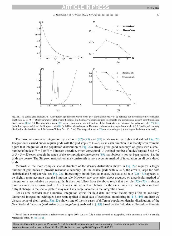
JID:PLREV AID:465 /REV [m3SC+; v 1.188; Prn:4/03/2014; 13:24] P.37 (1-59)
S. Petrovskii et al. / Physics of Life Reviews ••• (••••) •••–••• 37
Fig. 21. The coarse grid problem. (a) A monotone spatial distribution of the pest population density u(x) obtained for the dimensionless diffusioncoefficient D = 10−4. Other parameters along with the initial and boundary conditions used to generate one-dimensional density distributions arediscussed in [116]. (b) The integration error (76) arising from numerical integration of the distribution in (a) using the statistical rule (72)–(73)(solid line, open circle) and the Simpson rule (80) (solid line, closed square). The error is shown on the logarithmic scale. (c) A ‘multi-peak’ densitydistribution obtained for the diffusion coefficient D = 10−5. (d) The integration error (76) corresponding to (c), the legend is the same as in (b).
The error of numerical integration by methods (72)–(73) and (87) is shown in the right-hand side of Fig. 22.Integration is carried out on regular grids with the grid step size h = const in each direction. It is readily seen from thefigure that integration of the population distribution of Fig. 22a already gives good accuracy7 on grids with a smallnumber of nodes (N = 3 or N = 5 in each direction, which corresponds to the total number of nodes/traps as 3×3 = 9or 5×5 = 25) even though the range of the asymptotical convergence (89) has obviously not yet been reached, i.e. thegrids are coarse. The Simpson method remains consistently a more accurate method of integration on all consideredgrids.
Meanwhile, the more complex spatial structure of the density distribution shown in Fig. 22c requires a largernumber of grid nodes to provide reasonable accuracy. On the coarse grids with N = 3, the error is large for bothstatistical and Simpson rule; see Fig. 22d. Interestingly, in this particular case, the statistical rule (72)–(73) appears tobe slightly more accurate than the Simpson rule. However, any conclusion about accuracy on a particular method ofintegration is not reliable on coarse girds. It does not follow from the above result that the rule (72)–(73) is alwaysmore accurate on a coarse grid of 3 × 3 nodes. As we will see below, for the same numerical integration method,a slight change in the spatial pattern may result in a large increase in the integration error.
Let us now consider how numerical integration works for field data and what factors may affect its accuracy.Numerical integration techniques have been applied to field data of ecological monitoring in [115,119] and here wediscuss some of their results. Fig. 23a shows one of the six cases of different population density distributions of theNew Zealand flatworm (Arthurdendyus triangulatus) analyzed in [119] based on the field data collected by Murchie
7 Recall that in ecological studies a relative error of up to 50% (i.e. e ∼ 0.5) is often deemed as acceptable, while an error e < 0.3 is usuallyregarded as small, cf. [111,152].

JID:PLREV AID:465 /REV [m3SC+; v 1.188; Prn:4/03/2014; 13:24] P.38 (1-59)
38 S. Petrovskii et al. / Physics of Life Reviews ••• (••••) •••–•••
Fig. 22. The coarse grid problem in the 2D case. (a, c) Population density u(x, y) obtained from a mathematical model of population dynamics (seedetails in the text), (b, d) the corresponding integration error (76) shown on the logarithmic scale, N is the number of nodes in each direction x andy of a regular Cartesian grid. (a) A single peak population distribution typical for the values of the diffusion coefficient D ∼ 1 or larger. (b) Theintegration error for the statistical rule (solid line, open circle) and the Simpson rule (solid line, closed square) corresponding to (a). (c) A snapshotof a patchy population density distribution typical for D � 1. (d) The integration error corresponding to (c), the legend is the same as in (b).
Fig. 23. Numerical integration of field data on a coarse regular grid of 3 × 3 nodes, the nodes are shown as large black dots. (a) The populationdensity u(x, y) based on the field data collected in [100] (see also [119]). The two circled grid nodes fall into small patches of lower density. Sincethe density values at those locations are not representative (“outliers”), 2/9 of the total information is lost and hence numerical integration results ina large integration error. (b) The density function u(x, y) based on the field data by [5]; see details in the text. (For interpretation of the referencesto color in this figure, the reader is referred to the web version of this article.)
and Harrison [100]. The original data were collected with 121 traps installed at the nodes of a regular grid of 11 × 11nodes. First, the values of the population density available at the nodes of this fine grid were integrated in order toobtain the ‘true’ value of the population size. (In Fig. 23a, the population density is shown as a continuous function

JID:PLREV AID:465 /REV [m3SC+; v 1.188; Prn:4/03/2014; 13:24] P.39 (1-59)
S. Petrovskii et al. / Physics of Life Reviews ••• (••••) •••–••• 39
Table 1The approximated value Ia of the total population size and the integration error e on a regular grid of 3 × 3 nodes for the field data. The rowsmarked (a) and (b) correspond to the population density distributions shown in Figs. 23a and 23b, respectively. Ia and e are computed by thestatistical rule (72)–(73) (the columns I stat
a and estat) and by the Simpson rule (87) (the columns ISRa and eSR).
Case I I stata estat ISR
a eSR
(a) 544 289 0.469 247 0.545(b) 1980 1507 0.239 2332 0.178
u(x, y) using linear interpolation.) Then, a coarse grid of 3 × 3 = 9 nodes was generated by picking the first, sixthand eleventh nodes in each direction. The locations of those selected 9 traps on a coarse grid is shown in Fig. 23a bylarge black dots, the values of the population density at those locations were taken from the original grid. Finally, theapproximate value Ia of the population size was obtained by numerical integration over that coarse grid.
The values of Ia obtained with different integration rules [see case (a) in Table 1] were compared to the ‘true’ valueI in order to estimate the accuracy of the approach. Here we want to mention that the case shown in Fig. 23a wasthe one with the worst accuracy. For the other five population distributions analyzed in [119], the integration error onthe coarse 3 × 3 grid was consistently less than 35% and the Simpson rule was shown to be more accurate (with theintegration error less than 10% in three our of six cases). However, here we deliberately focus on the most difficultcase shown in Fig. 23a as it is instructive to understand the reasons resulting in the relatively large integration errorshown in Table 1.
First, we note that the larger error of the Simpson rule compared to the statistical rule (see Table 1, row (a)) clearlyindicates that the 3 × 3 integration grid is indeed coarse as on a fine grid it should have been otherwise; see Fig. 20.Secondly, consistent with our analysis above, the accuracy of integration is determined by the properties of the spatialpattern in the density distribution [119]. After a careful visual examination of Fig. 23a, it becomes clear that, on thecoarse grid, some information about the density function u(x, y) is lost as two out of nine grid nodes are located insidesmall patches where the density is significantly different (lower) from the density in the surrounding areas; those nodesare circled in the figure. Hence two out of the nine available local density values used for numerical integration willmake a misleading contribution to the integral Ia , no matter what integration technique is used. As a result, we have arelative integration error e ∼ 0.5 for both statistical and Simpson rules.
For the second example, Fig. 23b presents the field data from [5] where the insect species Pterostichus melanariuswas monitored with pitfall traps installed at the nodes of 15 × 15 regular Cartesian grid. The corresponding densitydistribution u(x, y) obtained as a linear interpolation of the local density values is shown in Fig. 23b. The idea ofour analysis is similar to the previous example, i.e. we obtain the ‘true’ value I of the population size by integratingthe data on the original fine grid, construct a coarse 3 × 3 grid as a relevant subset of grid nodes, and then obtain anapproximate value Ia by integrating the data on the coarse grid. Note that, in this case, the population distribution hasnot just one but several small patches of high density. Obviously, these small patches are unlikely to be well resolvedon a 3 × 3 grid. Hence the poor resolution of the pattern can be expected to contribute to the integration error. On theother hand, there is a large area inside the domain where the density, while rather low, is approximately homogeneous(shown in various shades of blue in Fig. 23b). The population density in this area is well-resolved on the grid of 3 × 3nodes and hence the contribution to the integral from this sub-domain is expected to be sufficiently accurate. Sincethe number of high-density patches is not large, we can therefore expect a reasonably small integration error on thecoarse grid. This heuristic argument is in agreement with the results of numerical integration; case (b) of Table 1shows that the relative error is less than 25%. Interestingly, as was shown in [115], an increase in the number of trapsfrom 3 × 3 to 9 × 9 does not significantly increase the accuracy of integration because small patches of high densityremain unresolved on those grids.
The above results lead us to the conclusion that, on a grid with a given number of nodes (traps), the accuracy of pestabundance evaluation is to a large extent determined by the properties of the spatial pattern in the density distribution.Therefore, the following simple classification can be offered:
(A) N (the number of nodes in each direction) is sufficiently large to make the grid fine for the given spatial densitydistribution, so the asymptotic error estimate (89) holds and the integration error is small.
(B) N is not large enough for the given spatial density distribution, so the grid is coarse and the asymptotic errorestimate (89) does not hold, however the integration error appears to be small.
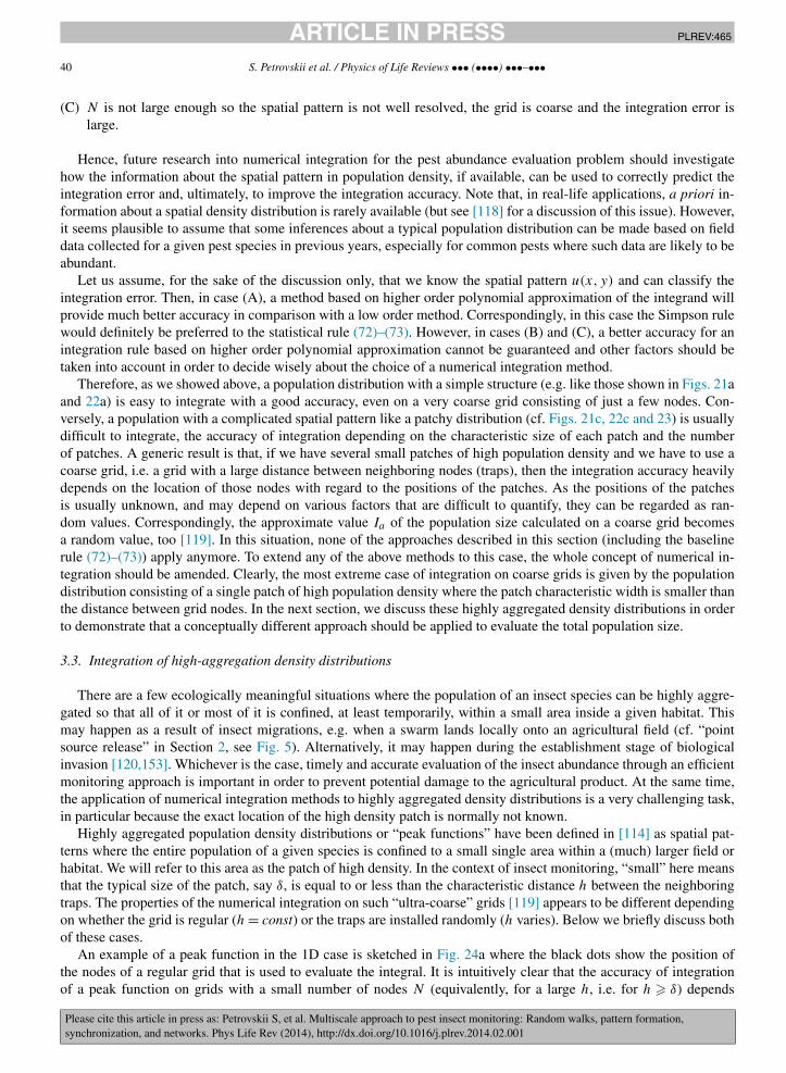
JID:PLREV AID:465 /REV [m3SC+; v 1.188; Prn:4/03/2014; 13:24] P.40 (1-59)
40 S. Petrovskii et al. / Physics of Life Reviews ••• (••••) •••–•••
(C) N is not large enough so the spatial pattern is not well resolved, the grid is coarse and the integration error islarge.
Hence, future research into numerical integration for the pest abundance evaluation problem should investigatehow the information about the spatial pattern in population density, if available, can be used to correctly predict theintegration error and, ultimately, to improve the integration accuracy. Note that, in real-life applications, a priori in-formation about a spatial density distribution is rarely available (but see [118] for a discussion of this issue). However,it seems plausible to assume that some inferences about a typical population distribution can be made based on fielddata collected for a given pest species in previous years, especially for common pests where such data are likely to beabundant.
Let us assume, for the sake of the discussion only, that we know the spatial pattern u(x, y) and can classify theintegration error. Then, in case (A), a method based on higher order polynomial approximation of the integrand willprovide much better accuracy in comparison with a low order method. Correspondingly, in this case the Simpson rulewould definitely be preferred to the statistical rule (72)–(73). However, in cases (B) and (C), a better accuracy for anintegration rule based on higher order polynomial approximation cannot be guaranteed and other factors should betaken into account in order to decide wisely about the choice of a numerical integration method.
Therefore, as we showed above, a population distribution with a simple structure (e.g. like those shown in Figs. 21aand 22a) is easy to integrate with a good accuracy, even on a very coarse grid consisting of just a few nodes. Con-versely, a population with a complicated spatial pattern like a patchy distribution (cf. Figs. 21c, 22c and 23) is usuallydifficult to integrate, the accuracy of integration depending on the characteristic size of each patch and the numberof patches. A generic result is that, if we have several small patches of high population density and we have to use acoarse grid, i.e. a grid with a large distance between neighboring nodes (traps), then the integration accuracy heavilydepends on the location of those nodes with regard to the positions of the patches. As the positions of the patchesis usually unknown, and may depend on various factors that are difficult to quantify, they can be regarded as ran-dom values. Correspondingly, the approximate value Ia of the population size calculated on a coarse grid becomesa random value, too [119]. In this situation, none of the approaches described in this section (including the baselinerule (72)–(73)) apply anymore. To extend any of the above methods to this case, the whole concept of numerical in-tegration should be amended. Clearly, the most extreme case of integration on coarse grids is given by the populationdistribution consisting of a single patch of high population density where the patch characteristic width is smaller thanthe distance between grid nodes. In the next section, we discuss these highly aggregated density distributions in orderto demonstrate that a conceptually different approach should be applied to evaluate the total population size.
3.3. Integration of high-aggregation density distributions
There are a few ecologically meaningful situations where the population of an insect species can be highly aggre-gated so that all of it or most of it is confined, at least temporarily, within a small area inside a given habitat. Thismay happen as a result of insect migrations, e.g. when a swarm lands locally onto an agricultural field (cf. “pointsource release” in Section 2, see Fig. 5). Alternatively, it may happen during the establishment stage of biologicalinvasion [120,153]. Whichever is the case, timely and accurate evaluation of the insect abundance through an efficientmonitoring approach is important in order to prevent potential damage to the agricultural product. At the same time,the application of numerical integration methods to highly aggregated density distributions is a very challenging task,in particular because the exact location of the high density patch is normally not known.
Highly aggregated population density distributions or “peak functions” have been defined in [114] as spatial pat-terns where the entire population of a given species is confined to a small single area within a (much) larger field orhabitat. We will refer to this area as the patch of high density. In the context of insect monitoring, “small” here meansthat the typical size of the patch, say δ, is equal to or less than the characteristic distance h between the neighboringtraps. The properties of the numerical integration on such “ultra-coarse” grids [119] appears to be different dependingon whether the grid is regular (h = const) or the traps are installed randomly (h varies). Below we briefly discuss bothof these cases.
An example of a peak function in the 1D case is sketched in Fig. 24a where the black dots show the position ofthe nodes of a regular grid that is used to evaluate the integral. It is intuitively clear that the accuracy of integrationof a peak function on grids with a small number of nodes N (equivalently, for a large h, i.e. for h � δ) depends
JID:PLREV AID:465 /REV [m3SC+; v 1.188; Prn:4/03/2014; 13:24] P.41 (1-59)
S. Petrovskii et al. / Physics of Life Reviews ••• (••••) •••–••• 41
Fig. 24. (a) An example of a 1D highly aggregated distribution of the population density u(x) (high density patch, peak function), black dots showthe position of the grid nodes. (b) The probability of obtaining an accurate estimate of the pest population size if traps are installed at nodes of aregular grid. (c) The probability of obtaining an accurate estimate of the pest population size using the integration rule (72)–(73) on a random gridof traps under the constraint that only a single trap falls into the high density patch.
on the peak width and peak location with respect to the grid nodes. In the worst case scenario, a narrow peak canfall entirely between two neighboring nodes of the grid and then the integration gives exactly zero, which is grosslymisrepresentative of the true population size. On the other hand, it is equally possible to find a peak location such thatintegration of the population density u(x) on the same regular grid would provide a very accurate answer [118].
Correspondingly, the following issues arise: (i) what is the minimum ‘critical’ number Nc of nodes/traps requiredto achieve desirable accuracy if a highly aggregated population density distribution u(x) of a given width δ is inte-grated on a 1D regular grid, and (ii) what is an appropriate measure of integration accuracy on a regular grid of trapswhere N < Nc? Following [114,119], we address these issues by introducing the concept of an ultra-coarse grid. Anultra-coarse grid is defined as a grid where the integration error is essentially a random variable because of insuffi-cient information (uncertainty) about the integrand function. When numerical integration is performed on ultra-coarsegrids, the integration error as such does not have much meaning as it can be very different for a slightly differentposition of the peak (which is unknown). Instead, one can calculate the probability p that the value of the error willremain smaller than the given tolerance τ , cf. Eq. (77).
It does not seem possible to calculate p analytically for an arbitrary population density u(x). However, we re-call that the spatial distribution of the population density appears as a result of movement of individual insects; seeSection 2.2. Depending on the type of the movement (e.g. diffusion or superdiffusion), that will add up to either thenormal distribution or the Cauchy distribution. Both distributions are dome-shaped so that the density profile aroundits maximum value (located at a certain x = xm) is obviously described as u(x) = u(xm) − u′′(xm)x2 + o(x2). Corre-spondingly, by neglecting the tail of the density profile (which does not affect the accuracy much, see [118]), we canapproximate u(x) with a square polynomial.
Based on the quadratic approximation of the peak function, the probability p(h) that the value of the integrationerror does not exceed τ was obtained in [114]. The exact shape of the graph p(h) depends on the chosen integrationrule, on δ and on τ ; the generic shape is shown in Fig. 24b. The probability p(h) appears to be a piecewise function ofthe grid step h; there exists a critical, threshold value hc such that p(h) ≡ 1 for any h� hc , and p(h) is a monotonouslydecreasing function for h > hc. It was also shown in [114] that the critical grid step size hc is a linear function of thepeak function’s width:
hc = αc(τ )δ, (90)
where the coefficient αc depends on the tolerance τ .In order to illustrate how this approach works, we consider a hypothetical aggregated population density distribu-
tion u(x) with the width δ, so that the corresponding probability p(h) is given by the curve shown in Fig. 24b. If thedata on local abundance are collected on a regular grid with the step size h0 > hc , for example, then our chance toevaluate the integral within the acceptable accuracy range τ is p(h0) ≈ 0.15. Therefore, for this grid with N0 ≈ 1/h0nodes, there is an 85% chance that the error of our evaluation will be larger than the maximum affordable error τ . Inother words, if this grid of traps is installed in ten similar fields, it is likely that in 8 cases out of 10 the obtained esti-mate of the pest population size will have little to do with reality. Clearly, this is a very low quality monitoring system.

JID:PLREV AID:465 /REV [m3SC+; v 1.188; Prn:4/03/2014; 13:24] P.42 (1-59)
42 S. Petrovskii et al. / Physics of Life Reviews ••• (••••) •••–•••
Consider now a regular grid with h1 < hc and the number of nodes N1 ≈ 1/h1. The error of integral evaluation isnow smaller than τ , no matter where the peak is located. The probability p(h) of getting the error within the accuracyrange e(N1) < τ is p(h1) = 1. In this case, in all ten fields the pest population size is evaluated meaningfully.
If the grid is not regular, e.g. some of the traps are misplaced, the integration accuracy may become worse [118].Let us consider the integration of a peak function on an irregular grid where the position of all the traps across thedomain is chosen randomly (according to a certain rule to ensure that the traps are distributed uniformly – now in thestatistical sense – across the whole area). Integration of a highly aggregated population density on random grids usingthe statistical rule (72)–(73) was studied in [44] both in 1D and 2D cases under an assumption that the total number oftraps is small, so that only one trap falls within the high density patch. Note that this assumption is very important inthe context of the real-life monitoring as it describes the existing typical constraints; see the beginning of Section 3.Under this assumption, in a similar way to the regular case, the grid is ultra-coarse because of the uncertainty of thepeak location, and an estimate of the total population size is a random variable.
The probability p to obtain an estimate with the error e < τ was calculated in [44] basing on the quadratic ap-proximation of the population density profile. An example of the probability p as a function of the number N of gridnodes is shown in Fig. 24c. Note that the function p(N) consists of two branches. The increasing branch reflects thebetter averaging of the error with an increase in N . The decreasing branch of the graph p(N) shows the (decreasing)probability to have exactly one trap inside the patch [44]; this range of N should therefore be regarded as unrealisticbecause of the constraints mentioned above. Correspondingly, under the assumption of a single trap within the highdensity patch, there is an optimum number Nmax of traps that provides the maximum probability pmax of obtaining anaccurate estimate. Interestingly, it appears that the maximum probability is always pmax < 1 [44].
The results revisited in this section demonstrate that the conventional conclusions that ecologists make about accu-racy of pest abundance evaluation should be regarded with care. Ecologists are well aware that there is uncertainty inthe estimation of the pest abundance, which may become worse as the number of samples decreases [18]. However, tothe best of our knowledge, the idea of handling the error of the evaluation as a random variable has not been discussedin the ecological literature so far. Under the conditions that only a small number of traps are available per field and ahighly aggregated population distribution is likely to occur, our results may eventually lead to a paradigm shift wherethe traditional ways to estimate the population abundance in individual fields give way to “probabilistic integration”across a group of fields or habitats with similar properties.
4. Landscape scale: synchronization and self-organization
The largest spatial scale in the problem of pest monitoring is the landscape scale that may include many agricul-tural fields as well as non-farmed habitats. Pest monitoring programs are usually region-wide or even nation-wide.For instance, aphids have been the focus of an intensive monitoring program in the U.K. Aphids rarely cause anysignificant damage by themselves but they are regarded as harmful species because of their high potential to transmitviruses to crops. In order to monitor aphid abundance, the U.K. Food and Environment Research Agency created amonitoring system consisting of dozens of traps installed at various locations across the country [104]. The systemwas set up in 2002, and for the first two years consisted of around a dozen traps in 4 geographically distinct regions(Scotland, North Yorkshire, East Anglia and Wiltshire). From 2004 onwards, the system has consisted of around 100traps in 8 regions; see Fig. 25.
Good understanding of trends and peculiarities in the trap counts is clearly important for providing timely andreliable information about pest abundance to crops growers. A visual inspection of the map shown in Fig. 25 imme-diately reveals that the trap counts at different locations do not seem to be independent as the date of the first catchof the pest insect appears to be correlated across a certain area. This indicates that aphid population numbers are notentirely independent either. A question thus arises as to how typical this situation is and whether it originates in thelandscape properties, in the weather conditions (e.g. seasonality) or in some inherent density-dependent populationself-regulation.
Environment is known to affect the population dynamics in space and time through a variety of specific factors suchas landscape structure [71,131], seasonality and solar cycles [155], weather conditions on both global and regionalscales [9,138,139], etc. In many cases, the population fluctuations in different habitats appear to be, to a certainextent, correlated; the phenomenon known as synchronization [85,87]. The example of aphids considered above istherefore by no means unique. There is increasing recognition that an efficient and reliable insect pest monitoring
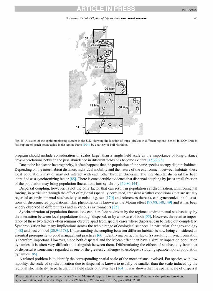
JID:PLREV AID:465 /REV [m3SC+; v 1.188; Prn:4/03/2014; 13:24] P.43 (1-59)
S. Petrovskii et al. / Physics of Life Reviews ••• (••••) •••–••• 43
Fig. 25. A sketch of the aphid monitoring system in the U.K. showing the location of traps (circles) in different regions (boxes) in 2009. Date isfirst capture of peach potato aphid in the region. From [104], by courtesy of Phil Northing.
program should include consideration of scales larger than a single field scale as the importance of long-distancecross-correlations between the pest abundance in different fields has become evident [15,22,23].
Due to the landscape heterogeneity, it often happens that the population of the same species occupy disjoint habitats.Depending on the inter-habitat distance, individual mobility and the nature of the environment between habitats, theselocal populations may or may not interact with each other through dispersal. The inter-habitat dispersal has beenidentified as a synchronizing factor [85]. There is considerable evidence that dispersal coupling by just a small fractionof the population may bring population fluctuations into synchrony [59,80,144].
Dispersal coupling, however, is not the only factor that can result in population synchronization. Environmentalforcing, in particular through the effect of regional (spatially correlated) transient weather conditions (that are usuallyregarded as environmental stochasticity or noise; e.g. see [170] and references therein), can synchronize the fluctua-tions of disconnected populations. This phenomenon is known as the Moran effect [97,98,140,149] and it has beenwidely observed in different taxa and in various environments [85].
Synchronization of population fluctuations can therefore be driven by the regional environmental stochasticity, bythe interaction between local populations through dispersal, or by a mixture of both [55]. However, the relative impor-tance of these two factors often remains obscure apart from special cases where dispersal can be ruled out completely.Synchronization has many implications across the whole range of ecological sciences, in particular, for agro-ecology[148] and pest control [20,94,178]. Understanding the coupling between different habitats is now being considered anessential prerequisite to good management practices [66]. Identifying particular factor(s) resulting in synchronizationis therefore important. However, since both dispersal and the Moran effect can have a similar impact on populationdynamics, it is often very difficult to distinguish between them. Differentiating the effects of stochasticity from thatof dispersal is sometimes regarded as one of the greatest challenges to ecologists studying spatiotemporal populationdynamics [85].
A related problem is to identify the corresponding spatial scale of the mechanisms involved. For species with lowmobility, the scale of synchronization due to dispersal is known to usually be smaller than the scale induced by theregional stochasticity. In particular, in a field study on butterflies [164] it was shown that the spatial scale of dispersal
JID:PLREV AID:465 /REV [m3SC+; v 1.188; Prn:4/03/2014; 13:24] P.44 (1-59)
44 S. Petrovskii et al. / Physics of Life Reviews ••• (••••) •••–•••
coupling is on the order of 5 km while population synchrony can be observed on much larger distances of up to200 km. The larger spatial scale of synchronization is therefore likely to be linked to regional stochasticity, althoughthis may not necessarily be true if insect dispersal is assisted by the wind [15].
Note that the large, landscape spatial scale of the insect monitoring problem allows for a different level of detailin the description of local populations. We no longer consider trap counts (like in Section 2) or population densitiesat particular locations (like in Section 3). Instead, each monitored unit, e.g. an agricultural field, is now describedby a single variable such as the total population size or the average density of a given pest species. In terms of themathematical framework, it means that we consider a discrete space – a lattice [7,95,146] or a network [68,150] –rather than a continuous one.
Let us consider the populations of a certain species dwelling in two fields, say, X and Y . The population cen-sus takes place at certain times, t1, . . . , tn (e.g. weekly, monthly or annually), and results in the two time-courses,X1, . . . ,Xn and Y1, . . . , Yn where Xi and Yi are the population sizes of the monitored species in fields X and Y , re-spectively, at time ti . The degree of synchronization between the two populations is usually quantified by the Pearsonproduct moment correlation coefficient:
r0(X,Y ) =∑n
i=1(Xi − μX)(Yi − μY )√(∑n
i=1(Xi − μX)2)(∑n
i=1(Yi − μY )2)
, (91)
where n is the length of the monitoring time-course and μX and μY are the sample means of the two time series, i.e.:
μX = 1
n
n∑i=1
Xi, μY = 1
n
n∑i=1
Yi. (92)
In order to demonstrate a practical application of this technique,8 to reveal its limitations and to discuss its pos-sible extension and/or modification, we now consider a case study [15]. The population of T. paludosa, a commonagricultural insect pest in the British Isles, was monitored over 15 years between 1980 and 1994 across a region inSouth-Western Scotland; see Fig. 26. The study covered the area of approximately 200 × 200 km2 with the inter-fielddistances varying between 2 and 200 km (Fig. 27).
Tipula paludosa is a univoltine insect species with adult emergence, under the typical U.K. weather conditions,between mid-August and mid-September. Adult T. paludosa are flying insects; however, their dispersal is thought tobe limited as females are poor fliers, emerging gravid and laying eggs within one day. The larval stages of T. paludosa,known as leatherjackets, are soil dwelling and relatively lacking in mobility.
An annual census of the population abundance was taken in mid-winter (when the species is in the larval stage)in each of 38 fields shown in the map. This resulted in 38 time-courses, each containing 15 datapoints, i.e. values ofthe average population density over 15 years. The correlation coefficient r0 was then calculated for all possible pairsof these time-courses. The results are shown in Fig. 28. We observe that the dependence of r0 on distance betweenfields exhibits a clear intermittent behavior with: some fields being strongly positively correlated (synchronized) up todistance of 150–170 km, some fields being significantly negatively correlated, and some fields (including cases wherethe fields are situated very close to each other) being not correlated at all. A general trend in correlation strengthvs distance can be revealed using linear regression analysis (solid line in Fig. 28), which shows a slow decay. Wetherefore conclude that, as such, the distance between fields does not provide sufficient information to decide whetherthe populations of two fields are likely to be synchronized.
A better understanding of the system’s properties can be achieved if the correlation strength is linked to the actualposition of the fields. Fig. 29 shows the location of all 38 fields where those that are significantly correlated, in thestatistical sense, are connected by a line. Interestingly, the observed network exhibits anisotropic properties with morecorrelated pairs situated along the North-West to South-East direction than on other bearings. Since the terrain doesnot seem to possess any clear directional structure, one can hypothesize that the asymmetry in the network shown inFig. 29 may have appeared because of the impact of the wind. Indeed, having considered the weather data (location ofthe weather stations is shown in Fig. 26 by the flag), a considerable similarity between the structure of the inter-fieldcorrelations and the prevailing wind directions was discovered [15].
8 Sometimes it may be necessary first to remove the effects of density dependence from the original data before calculating the cross-correlationcoefficient (91) in order to make sure that the individual time series are serially independent.
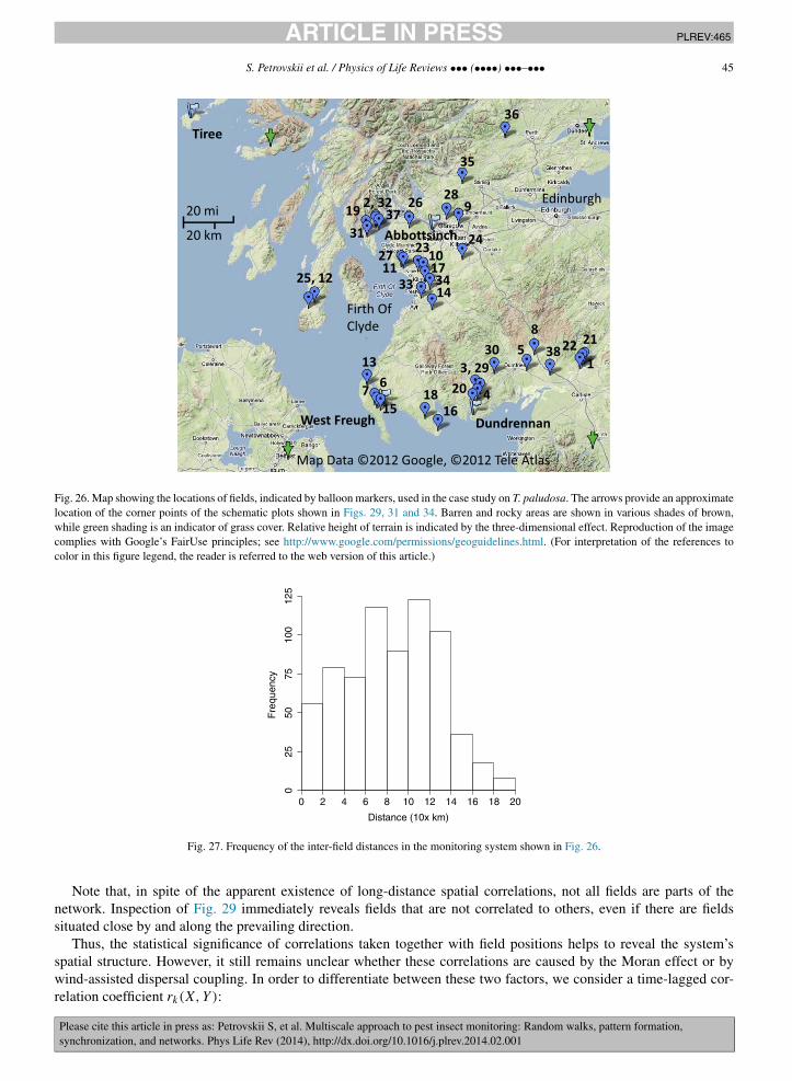
JID:PLREV AID:465 /REV [m3SC+; v 1.188; Prn:4/03/2014; 13:24] P.45 (1-59)
S. Petrovskii et al. / Physics of Life Reviews ••• (••••) •••–••• 45
Fig. 26. Map showing the locations of fields, indicated by balloon markers, used in the case study on T. paludosa. The arrows provide an approximatelocation of the corner points of the schematic plots shown in Figs. 29, 31 and 34. Barren and rocky areas are shown in various shades of brown,while green shading is an indicator of grass cover. Relative height of terrain is indicated by the three-dimensional effect. Reproduction of the imagecomplies with Google’s FairUse principles; see http://www.google.com/permissions/geoguidelines.html. (For interpretation of the references tocolor in this figure legend, the reader is referred to the web version of this article.)
Fig. 27. Frequency of the inter-field distances in the monitoring system shown in Fig. 26.
Note that, in spite of the apparent existence of long-distance spatial correlations, not all fields are parts of thenetwork. Inspection of Fig. 29 immediately reveals fields that are not correlated to others, even if there are fieldssituated close by and along the prevailing direction.
Thus, the statistical significance of correlations taken together with field positions helps to reveal the system’sspatial structure. However, it still remains unclear whether these correlations are caused by the Moran effect or bywind-assisted dispersal coupling. In order to differentiate between these two factors, we consider a time-lagged cor-relation coefficient rk(X,Y ):
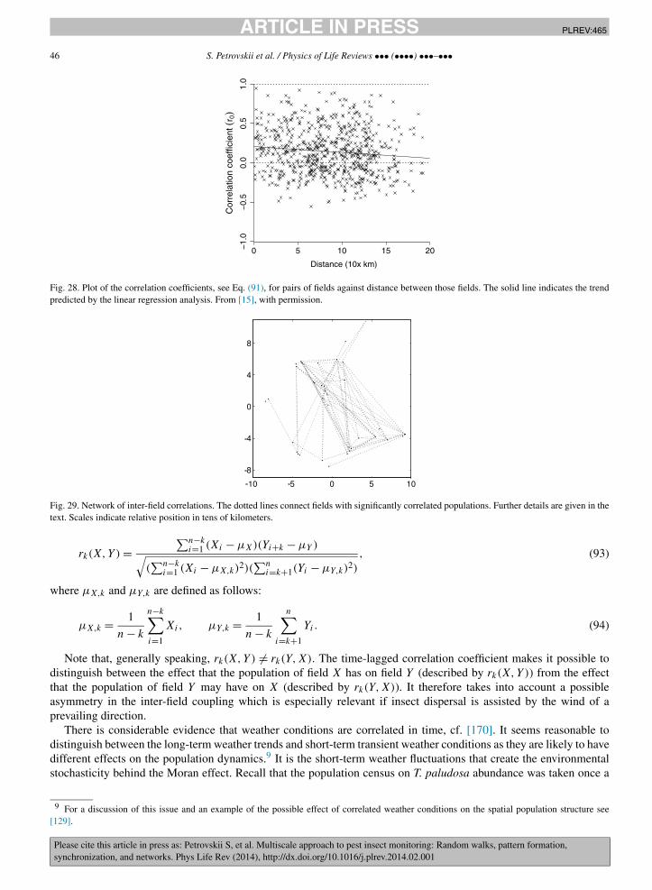
JID:PLREV AID:465 /REV [m3SC+; v 1.188; Prn:4/03/2014; 13:24] P.46 (1-59)
46 S. Petrovskii et al. / Physics of Life Reviews ••• (••••) •••–•••
Fig. 28. Plot of the correlation coefficients, see Eq. (91), for pairs of fields against distance between those fields. The solid line indicates the trendpredicted by the linear regression analysis. From [15], with permission.
Fig. 29. Network of inter-field correlations. The dotted lines connect fields with significantly correlated populations. Further details are given in thetext. Scales indicate relative position in tens of kilometers.
rk(X,Y ) =∑n−k
i=1 (Xi − μX)(Yi+k − μY )√(∑n−k
i=1 (Xi − μX,k)2)(∑n
i=k+1(Yi − μY,k)2)
, (93)
where μX,k and μY,k are defined as follows:
μX,k = 1
n − k
n−k∑i=1
Xi, μY,k = 1
n − k
n∑i=k+1
Yi. (94)
Note that, generally speaking, rk(X,Y ) �= rk(Y,X). The time-lagged correlation coefficient makes it possible todistinguish between the effect that the population of field X has on field Y (described by rk(X,Y )) from the effectthat the population of field Y may have on X (described by rk(Y,X)). It therefore takes into account a possibleasymmetry in the inter-field coupling which is especially relevant if insect dispersal is assisted by the wind of aprevailing direction.
There is considerable evidence that weather conditions are correlated in time, cf. [170]. It seems reasonable todistinguish between the long-term weather trends and short-term transient weather conditions as they are likely to havedifferent effects on the population dynamics.9 It is the short-term weather fluctuations that create the environmentalstochasticity behind the Moran effect. Recall that the population census on T. paludosa abundance was taken once a
9 For a discussion of this issue and an example of the possible effect of correlated weather conditions on the spatial population structure see[129].

JID:PLREV AID:465 /REV [m3SC+; v 1.188; Prn:4/03/2014; 13:24] P.47 (1-59)
S. Petrovskii et al. / Physics of Life Reviews ••• (••••) •••–••• 47
Fig. 30. Plots of correlation coefficients r1 for pairs of distinct fields against distance between those fields calculated using a time-lag of 1 year,cf. Eq. (93) with k = 1. The solid line indicates the trend as predicted by linear regression analysis. From [15], with permission.
Fig. 31. Network of inter-field correlations subject to a one year delay. The lines connect fields between which significant relationships exist. Thered section of each line emanates from the influencing field, the blue section terminates at the influenced field. Further details are given in the text.Scales indicate relative position in tens of kilometers. (For interpretation of the references to color in this figure legend, the reader is referred to theweb version of this article.)
year. It is unlikely that synchronization due to the impact of stochasticity is subject to such a long delay. Therefore, ifthe synchronization pattern seen in Figs. 28 and 29 is caused by stochasticity, it is unlikely to be seen in the behaviorof the time-lagged correlation coefficient rk even for the shortest lag of k = 1.
In contrast, if the synchronization pattern is caused by dispersal coupling, it is likely to be captured by the coeffi-cient rk . The annual population census was taken in mid-winter. Dispersal is primarily associated with the flying stageof the insect species that occurs in late August/early September. Therefore, the effect of dispersal will not be seen inthe census until the next year. The effect of delay is likely to be felt more strongly if dispersal is asymmetric (whichis clearly the case of wind-assisted dispersal), i.e. field X delegates a fraction of its population to field Y but not viceversa.
We begin with the case where the time-lag is one year, k = 1, which seems to be justified by the species traits,i.e. by the fact that it produces exactly one generation per year. The correlation coefficient r1 vs inter-field distancecalculated for all pairs of fields used in the study is shown in Fig. 30. Time-lagged correlation strength vs distancetherefore exhibits an intermittent behavior roughly similar to that observed on the non-lagged case (cf. Fig. 28). Oneimportant difference, however, is that the number of fields that are negatively correlated is considerably larger in thetime-lagged case.
The spatial structure of the correlations is shown in Fig. 31. It is readily seen that all correlated fields are connectedinto a network. Since, as we have argued above, in the time-lagged case the correlations are likely to be the result ofinter-field coupling by dispersal, the structure shown in Fig. 31 is the network of T. paludosa dispersal over the study
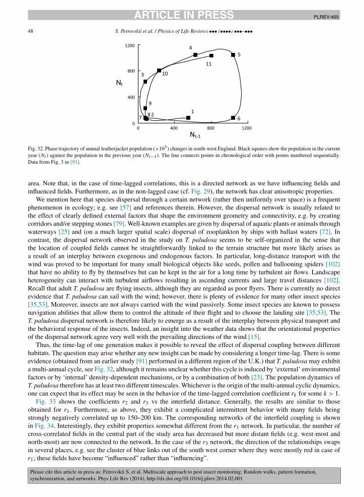
JID:PLREV AID:465 /REV [m3SC+; v 1.188; Prn:4/03/2014; 13:24] P.48 (1-59)
48 S. Petrovskii et al. / Physics of Life Reviews ••• (••••) •••–•••
Fig. 32. Phase trajectory of annual leatherjacket population (×103) changes in south-west England. Black squares show the population in the currentyear (Nt ) against the population in the previous year (Nt−1). The line connects points in chronological order with points numbered sequentially.Data from Fig. 3 in [91].
area. Note that, in the case of time-lagged correlations, this is a directed network as we have influencing fields andinfluenced fields. Furthermore, as in the non-lagged case (cf. Fig. 29), the network has clear anisotropic properties.
We mention here that species dispersal through a certain network (rather then uniformly over space) is a frequentphenomenon in ecology; e.g. see [57] and references therein. However, the dispersal network is usually related tothe effect of clearly defined external factors that shape the environment geometry and connectivity, e.g. by creatingcorridors and/or stepping stones [79]. Well-known examples are given by dispersal of aquatic plants or animals throughwaterways [25] and (on a much larger spatial scale) dispersal of zooplankton by ships with ballast waters [72]. Incontrast, the dispersal network observed in the study on T. paludosa seems to be self-organized in the sense thatthe location of coupled fields cannot be straightforwardly linked to the terrain structure but more likely arises asa result of an interplay between exogenous and endogenous factors. In particular, long-distance transport with thewind was proved to be important for many small biological objects like seeds, pollen and ballooning spiders [102]that have no ability to fly by themselves but can be kept in the air for a long time by turbulent air flows. Landscapeheterogeneity can interact with turbulent airflows resulting in ascending currents and large travel distances [102].Recall that adult T. paludosa are flying insects, although they are regarded as poor flyers. There is currently no directevidence that T. paludosa can sail with the wind; however, there is plenty of evidence for many other insect species[35,53]. Moreover, insects are not always carried with the wind passively. Some insect species are known to possessnavigation abilities that allow them to control the altitude of their flight and to choose the landing site [35,53]. TheT. paludosa dispersal network is therefore likely to emerge as a result of the interplay between physical transport andthe behavioral response of the insects. Indeed, an insight into the weather data shows that the orientational propertiesof the dispersal network agree very well with the prevailing directions of the wind [15].
Thus, the time-lag of one generation makes it possible to reveal the effect of dispersal coupling between differenthabitats. The question may arise whether any new insight can be made by considering a longer time-lag. There is someevidence (obtained from an earlier study [91] performed in a different region of the U.K.) that T. paludosa may exhibita multi-annual cycle, see Fig. 32, although it remains unclear whether this cycle is induced by ‘external’ environmentalfactors or by ‘internal’ density-dependent mechanisms, or by a combination of both [23]. The population dynamics ofT. paludosa therefore has at least two different timescales. Whichever is the origin of the multi-annual cyclic dynamics,one can expect that its effect may be seen in the behavior of the time-lagged correlation coefficient rk for some k > 1.
Fig. 33 shows the coefficients r2 and r3 vs the interfield distance. Generally, the results are similar to thoseobtained for r1. Furthermore, as above, they exhibit a complicated intermittent behavior with many fields beingstrongly negatively correlated up to 150–200 km. The corresponding networks of the interfield coupling is shownin Fig. 34. Interestingly, they exhibit properties somewhat different from the r1 network. In particular, the number ofcross-correlated fields in the central part of the study area has decreased but more distant fields (e.g. west-most andnorth-most) are now connected to the network. In the case of the r3 network, the direction of the relationships swapsin several places, e.g. see the cluster of blue links out of the south west corner where they were mostly red in case ofr1; these fields have become “influenced” rather than “influencing”.
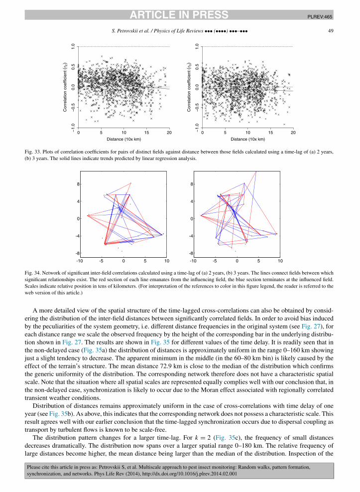
JID:PLREV AID:465 /REV [m3SC+; v 1.188; Prn:4/03/2014; 13:24] P.49 (1-59)
S. Petrovskii et al. / Physics of Life Reviews ••• (••••) •••–••• 49
Fig. 33. Plots of correlation coefficients for pairs of distinct fields against distance between those fields calculated using a time-lag of (a) 2 years,(b) 3 years. The solid lines indicate trends predicted by linear regression analysis.
Fig. 34. Network of significant inter-field correlations calculated using a time-lag of (a) 2 years, (b) 3 years. The lines connect fields between whichsignificant relationships exist. The red section of each line emanates from the influencing field, the blue section terminates at the influenced field.Scales indicate relative position in tens of kilometers. (For interpretation of the references to color in this figure legend, the reader is referred to theweb version of this article.)
A more detailed view of the spatial structure of the time-lagged cross-correlations can also be obtained by consid-ering the distribution of the inter-field distances between significantly correlated fields. In order to avoid bias inducedby the peculiarities of the system geometry, i.e. different distance frequencies in the original system (see Fig. 27), foreach distance range we scale the observed frequency by the height of the corresponding bar in the underlying distribu-tion shown in Fig. 27. The results are shown in Fig. 35 for different values of the time delay. It is readily seen that inthe non-delayed case (Fig. 35a) the distribution of distances is approximately uniform in the range 0–160 km showingjust a slight tendency to decrease. The apparent minimum in the middle (in the 60–80 km bin) is likely caused by theeffect of the terrain’s structure. The mean distance 72.9 km is close to the median of the distribution which confirmsthe generic uniformity of the distribution. The corresponding network therefore does not have a characteristic spatialscale. Note that the situation where all spatial scales are represented equally complies well with our conclusion that, inthe non-delayed case, synchronization is likely to occur due to the Moran effect associated with regionally correlatedtransient weather conditions.
Distribution of distances remains approximately uniform in the case of cross-correlations with time delay of oneyear (see Fig. 35b). As above, this indicates that the corresponding network does not possess a characteristic scale. Thisresult agrees well with our earlier conclusion that the time-lagged synchronization occurs due to dispersal coupling astransport by turbulent flows is known to be scale-free.
The distribution pattern changes for a larger time-lag. For k = 2 (Fig. 35c), the frequency of small distancesdecreases dramatically. The distribution now spans over a larger spatial range 0–180 km. The relative frequency oflarge distances become higher, the mean distance being larger than the median of the distribution. Inspection of the
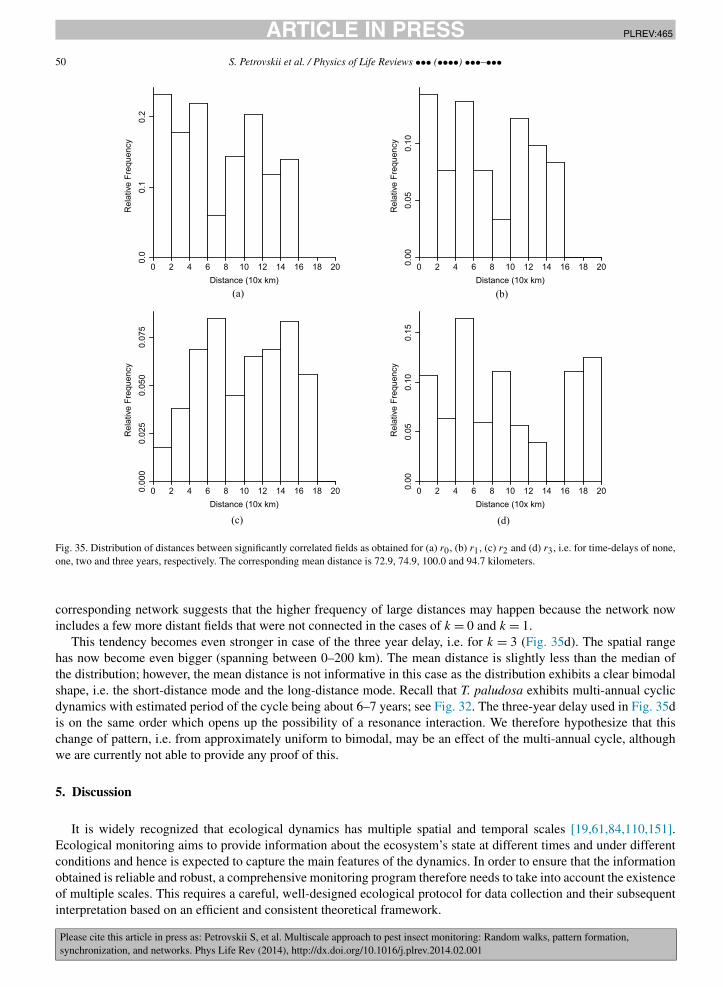
JID:PLREV AID:465 /REV [m3SC+; v 1.188; Prn:4/03/2014; 13:24] P.50 (1-59)
50 S. Petrovskii et al. / Physics of Life Reviews ••• (••••) •••–•••
Fig. 35. Distribution of distances between significantly correlated fields as obtained for (a) r0, (b) r1, (c) r2 and (d) r3, i.e. for time-delays of none,one, two and three years, respectively. The corresponding mean distance is 72.9, 74.9, 100.0 and 94.7 kilometers.
corresponding network suggests that the higher frequency of large distances may happen because the network nowincludes a few more distant fields that were not connected in the cases of k = 0 and k = 1.
This tendency becomes even stronger in case of the three year delay, i.e. for k = 3 (Fig. 35d). The spatial rangehas now become even bigger (spanning between 0–200 km). The mean distance is slightly less than the median ofthe distribution; however, the mean distance is not informative in this case as the distribution exhibits a clear bimodalshape, i.e. the short-distance mode and the long-distance mode. Recall that T. paludosa exhibits multi-annual cyclicdynamics with estimated period of the cycle being about 6–7 years; see Fig. 32. The three-year delay used in Fig. 35dis on the same order which opens up the possibility of a resonance interaction. We therefore hypothesize that thischange of pattern, i.e. from approximately uniform to bimodal, may be an effect of the multi-annual cycle, althoughwe are currently not able to provide any proof of this.
5. Discussion
It is widely recognized that ecological dynamics has multiple spatial and temporal scales [19,61,84,110,151].Ecological monitoring aims to provide information about the ecosystem’s state at different times and under differentconditions and hence is expected to capture the main features of the dynamics. In order to ensure that the informationobtained is reliable and robust, a comprehensive monitoring program therefore needs to take into account the existenceof multiple scales. This requires a careful, well-designed ecological protocol for data collection and their subsequentinterpretation based on an efficient and consistent theoretical framework.
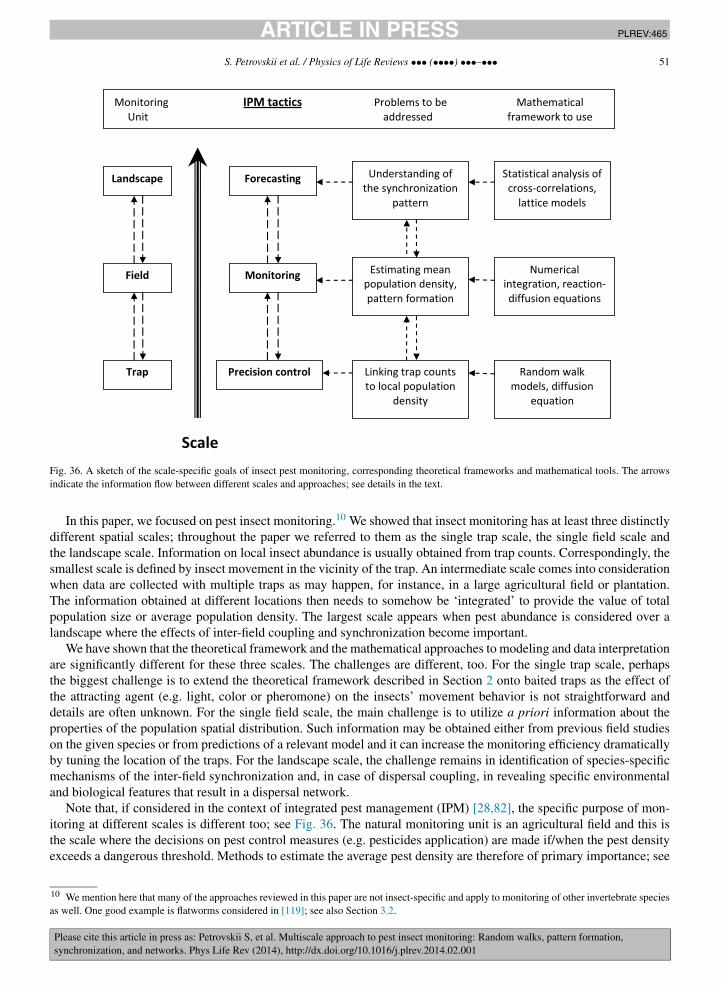
JID:PLREV AID:465 /REV [m3SC+; v 1.188; Prn:4/03/2014; 13:24] P.51 (1-59)
S. Petrovskii et al. / Physics of Life Reviews ••• (••••) •••–••• 51
Fig. 36. A sketch of the scale-specific goals of insect pest monitoring, corresponding theoretical frameworks and mathematical tools. The arrowsindicate the information flow between different scales and approaches; see details in the text.
In this paper, we focused on pest insect monitoring.10 We showed that insect monitoring has at least three distinctlydifferent spatial scales; throughout the paper we referred to them as the single trap scale, the single field scale andthe landscape scale. Information on local insect abundance is usually obtained from trap counts. Correspondingly, thesmallest scale is defined by insect movement in the vicinity of the trap. An intermediate scale comes into considerationwhen data are collected with multiple traps as may happen, for instance, in a large agricultural field or plantation.The information obtained at different locations then needs to somehow be ‘integrated’ to provide the value of totalpopulation size or average population density. The largest scale appears when pest abundance is considered over alandscape where the effects of inter-field coupling and synchronization become important.
We have shown that the theoretical framework and the mathematical approaches to modeling and data interpretationare significantly different for these three scales. The challenges are different, too. For the single trap scale, perhapsthe biggest challenge is to extend the theoretical framework described in Section 2 onto baited traps as the effect ofthe attracting agent (e.g. light, color or pheromone) on the insects’ movement behavior is not straightforward anddetails are often unknown. For the single field scale, the main challenge is to utilize a priori information about theproperties of the population spatial distribution. Such information may be obtained either from previous field studieson the given species or from predictions of a relevant model and it can increase the monitoring efficiency dramaticallyby tuning the location of the traps. For the landscape scale, the challenge remains in identification of species-specificmechanisms of the inter-field synchronization and, in case of dispersal coupling, in revealing specific environmentaland biological features that result in a dispersal network.
Note that, if considered in the context of integrated pest management (IPM) [28,82], the specific purpose of mon-itoring at different scales is different too; see Fig. 36. The natural monitoring unit is an agricultural field and this isthe scale where the decisions on pest control measures (e.g. pesticides application) are made if/when the pest densityexceeds a dangerous threshold. Methods to estimate the average pest density are therefore of primary importance; see
10 We mention here that many of the approaches reviewed in this paper are not insect-specific and apply to monitoring of other invertebrate speciesas well. One good example is flatworms considered in [119]; see also Section 3.2.

JID:PLREV AID:465 /REV [m3SC+; v 1.188; Prn:4/03/2014; 13:24] P.52 (1-59)
52 S. Petrovskii et al. / Physics of Life Reviews ••• (••••) •••–•••
Section 3. However, these methods use the information obtained locally from trap counts collected by a given trap;therefore, accurate estimation of the local density is an essential prerequisite. The forecasting done on the landscapescale aims to observe the regional tendencies in pest development. It also helps to identify the location of fields wherepotentially dangerous pest development is likely to take place (as well as, in principle, the timing of those events; seeFig. 25).
It is clear from the above that the information obtained at different scales is not independent. There are certain‘information flows’ between the scales. Precision of the local density estimate affects the field-scale accuracy ofthe average density estimate. In turn, as the information on average population density is used to reveal regionalcross-field correlations, it can affect the conclusions drawn on the landscape scale. Understanding of the processesand phenomena that can affect the accuracy of monitoring at the single-field scale is therefore crucial for insect pestmonitoring as a whole. One such phenomenon is pattern formation where the distribution of the pest populationdensity over space can become prominently heterogeneous due to the impact of some environmental and/or biologicalfactors. For instance, a heterogeneous insect distribution can be expected to emerge as a likely response to spatiallysynchronized fruit production observed in large orchards [148]. In Section 3, we showed that the accuracy of theaverage density estimate in the single field problem can be improved significantly (or the number of traps can bedecreased) if some a priori information is available about the spatial pattern. In other words, once the properties ofthe spatial pattern are known, it often becomes possible to draw conclusions about the population density at particularlocations. This additional information can then be used to significantly increase the accuracy of the local densityestimate at the single trap scale.
Thus, pattern formation at the intermediate, single-field level provides coupling between different spatial scales.Pattern formation in population dynamics is a complicated phenomenon that has been a focus of intensive researchfor a few decades [107,110,88]. It can be of different origins and controlled by different factors [6,60,89,108,147].One factor that seems to be particularly relevant to pattern formation in the agricultural context is the geometry of thedomain but the effects of the field shape seem to be largely overlooked in standard agricultural practices. Indeed, thevalue of a farm field often depends on its area but rarely on its shape. However, theory predicts (see below) that theproperties of the pattern can depend both on the size and shape of the domain. Hence, the efficiency of pest monitoring(which, in its turn, can greatly affect costs of crops growing, cf. Section 1) can be significantly different in fields ofdifferent shape, or else fields of different shape may require a different monitoring protocol.
In the theoretical perspective, there are a few situations where the effects of shape either are known or can bereadily seen. For the simplest example, let us consider a single-species population U(r, t) that multiplies according tothe logistic growth, f (U) = αU(1 − U
K), and diffuses inside a 2D domain of rectangular shape:
∂U(r, t)∂t
= D∇2U(r, t) + f (U) ≈ D∇2U(r, t) + αU(r, t),
r = (x, y), 0 < x < Lx, 0 < y < Ly, (95)
where we have assumed, for the sake of simplicity, that U � K and hence the growth rate is approximately linear,f (U) ≈ αU . We also assume that the environment outside of the domain is hostile so that the condition at the domainboundary Λ is of Dirichlet type, U(r ∈ Λ, t) = 0.
The linearized equation (95) can be readily solved by the method of variable separation [37]. Interestingly, thesolution appears to have different properties depending on how large the domain is in the x and y directions. Namely,the solution is decreasing for:
α − Dπ2(
1
L2x
+ 1
L2y
)< 0, (96)
which will eventually lead to population extinction, and is increasing otherwise. Obviously, for fixed values of α andD, it means that the population can only survive if both Lx and Ly are large enough. In particular, it means that thepopulation will survive in a square domain L × L for:
L > Lcr = π
(2D
)1/2
, (97)
α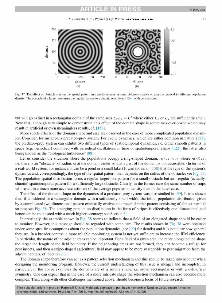
JID:PLREV AID:465 /REV [m3SC+; v 1.188; Prn:4/03/2014; 13:24] P.53 (1-59)
S. Petrovskii et al. / Physics of Life Reviews ••• (••••) •••–••• 53
Fig. 37. The effect of obstacle size on the spatial pattern in a predator–prey system. Different shades of grey correspond to different populationdensity. The obstacle of a larger size turns the regular pattern to a chaotic one. From [158], with permissions.
but will go extinct in a rectangular domain of the same area LxLy = L2 where either Lx or Ly are sufficiently small.Note that, although very simple to demonstrate, this effect of the domain shape is sometimes overlooked which mayresult in artificial or even meaningless results, cf. [156].
More subtle effects of the domain shape and size are observed in the case of more complicated population dynam-ics. Consider, for instance, a predator–prey system. For cyclic dynamics, which are rather common in nature [152],the predator–prey system can exhibit two different types of spatiotemporal dynamics, i.e. either smooth patterns inspace (e.g. periodical) combined with periodical oscillations in time or spatiotemporal chaos [122], the latter alsobeing known as the “biological turbulence” [88].
Let us consider the situation where the populations occupy a ring-shaped domain, r0 < r < r1 where r0 � r1,i.e. there is an “obstacle” of radius r0 at the domain center so that a part of the domain is not accessible. (In terms ofa real-world system, for instance, it can be a pond or a small lake.) It was shown in [158] that the type of the system’sdynamics and, correspondingly, the type of the spatial pattern then depends on the radius of the obstacle; see Fig. 37.The population spatial distribution forms a regular target-like pattern for a small obstacle but an irregular (actually,chaotic) spatiotemporal pattern for a sufficiently large obstacle. Clearly, in the former case the same number of trapswill result in a much more accurate estimate of the average population density than in the latter case.
The effect of the domain shape on the dynamics of a predator–prey system was also studied in [99]. It was shownthat, if considered in a rectangular domain with a sufficiently small width, the initial population distribution givenby a complicated two-dimensional pattern eventually evolves to a much simpler pattern consisting of almost parallelstripes; see Fig. 38. The emerging population distribution in the form of stripes is effectively one-dimensional andhence can be monitored with a much higher accuracy; see Section 3.
Interestingly, the example shown in Fig. 38 seems to indicate that a field of an elongated shape should be easierto monitor. However, this message should be regarded with some care. The results shown in Fig. 38 were obtainedunder some specific assumptions about the population dynamics (see [99] for details) and it is not clear how generalthey are. In a broader context, a more reliable monitoring system is not yet sufficient to increase the IPM efficiency.In particular, the nature of the adjoint areas can be important. For a field of a given area, the more elongated the shapethe larger the length of the field boundary. If the neighboring areas are not farmed, they can become a refuge forpest insects, and then a stripe-shaped agricultural field may appear to be more susceptible to pest migration from theadjoint habitats, cf. Section 2.3.
The domain shape therefore can act as a pattern selection mechanism and this should be taken into account whendesigning the monitoring program. However, the current understanding of this issue is meager and incomplete. Inparticular, in the above examples the domains are of a simple shape, i.e. either rectangular or with a cylindricalsymmetry. One can expect that in the case of a more intricate shape the selection mechanism can also become morecomplex. That, along with other challenges mentioned above, should become a focus of future research.

JID:PLREV AID:465 /REV [m3SC+; v 1.188; Prn:4/03/2014; 13:24] P.54 (1-59)
54 S. Petrovskii et al. / Physics of Life Reviews ••• (••••) •••–•••
Fig. 38. The population density of prey in a predator–prey system shown for three equidistant moments. Different shades of grey correspond todifferent population density. As the time increases (from left to right), the irregular 2D pattern converges to an effectively 1D system of planewaves. From [99], with permissions.
Acknowledgements
The authors are thankful to Rod Blackshaw (Plymouth) for fruitful and stimulating discussions of the topic. Helpfuldiscussions with Larissa Collins (FERA, Sand Hutton) are appreciated. The authors also acknowledge useful discus-sions of Sections 1 and 3 with Nina Embleton (Birmingham) and Section 2.5 with Danish Ahmed (Leicester). ThiloGross (Bristol) read the manuscript and made many comments aimed to improve the manuscript clarity. This workwas supported by The Leverhulme Trust through grant F/00-568/X. S.P. gratefully acknowledges the support given bythe University of Leicester in granting an academic study leave which was essential for completion of this work.
References
[1] Abramowitz M, Stegun IA. Handbook of mathematical functions. Washington: National Bureau of Standards; 1972.[2] Ahmed DA. Stochastic and mean-field approaches for trap counts modelling and interpretation. PhD thesis, Leicester: University of Leicester;
2014.[3] Ahmed DA, Bearup D, Petrovskii SV. Time-dependent diffusion as a mean-field counterpart of Levy-type random walk. Math Model Nat
Phenom 2014 [submitted for publication].[4] Alavanja MCR, Ross MK, Bonner MR. Increased cancer burden among pesticide applicators and others due to pesticide exposure. CA
Cancer J Clin 2013;62(2):120–42.[5] Alexander CJ, Holland JM, Winder L, Woolley C, Perry JN. Performance of sampling strategies in the presence of known spatial patterns.
Ann Appl Biol 2005;146:361–70.[6] Alonso D, Bartumeus F, Catalan J. Mutual interference between predators can give rise to Turing spatial patterns. Ecology 2002;83:28–34.[7] Allen JC, Schaffer WM, Rosko D. Chaos reduces species extinction by amplifying local population noise. Nature 1993;364:229–32.[8] Alyokhin A, Baker M, Mota-Sanchez D, Dively G, Grafius E. Colorado potato beetle resistance to insecticides. Am J Potato Res
2008;85:395–413.[9] Baars MA, Van Dijk TS. Population dynamics of two carabid beetles at a Dutch heathland. I. Subpopulation fluctuations in relation to weather
and dispersal. J Anim Ecol 1984;53:375–88.[10] Balescu R. Equilibrium and nonequilibrium statistical mechanics. New York: John Wiley; 1975.[11] Barclay HJ. Modelling the effects of population aggregation on the efficiency of insect pest control. Res Popul Ecol 1992;34:131–41.[12] Barenblatt GI. Scaling, self-similarity, and intermediate asymptotics. Cambridge: Cambridge University Press; 1996.[13] Bartumeus F, Catalan J, Viswanathan GM, Raposo EP, da Luz MGE. The influence of turning angles on the success of non-oriented animal
searches. J Theor Biol 2008;252:43–55.

JID:PLREV AID:465 /REV [m3SC+; v 1.188; Prn:4/03/2014; 13:24] P.55 (1-59)
S. Petrovskii et al. / Physics of Life Reviews ••• (••••) •••–••• 55
[14] Bearup D, Petrovskaya NB, Petrovskii SV. Some analytical and numerical approaches to understanding trap counts resulting from pest insectimmigration. Math Biosci 2014 [submitted for publication].
[15] Bearup D, Petrovskii SV, Blackshaw R, Hastings A. Synchronized dynamics of Tipula paludosa metapopulation in a South-Western Scotlandagroecosystem: linking pattern to process. Am Nat 2013;182:393–409.
[16] Benhamou S. How many animals really do the Lévy walk?. Ecology 2007;88:1962–9.[17] Berg HC. Random walks in biology. Princeton: Princeton University Press; 1983.[18] Binns MR, Nyrop JP, Van Der Werf W. Sampling and monitoring in crop protection: the theoretical basis for designing practical decision
guides. Wallingford: CABI Publishing; 2000.[19] Bisigato AJ, Villagra PE, Ares JO, Rossi BE. Vegetation heterogeneity in Monte Desert ecosystems: a multi-scale approach linking patterns
and processes. J Arid Environ 2009;73:182–91.[20] Blackshaw RP. The annual leatherjacket survey in Northern Ireland 1965–1982, and some factors affecting populations. Plant Pathol
1983;32:345–9.[21] Blackshaw RP. Personal communication.[22] Blackshaw RP, Vernon RS. Spatiotemporal stability of two beetle populations in non-farmed habitats in an agricultural landscape. J Appl
Ecol 2006;43:680–9.[23] Blackshaw RP, Petrovskii SV. Limitation and regulation of ecological populations: a meta-analysis of Tipula paludosa field data. Math Model
Nat Phenom 2007;2(4):46–62.[24] Boag B, Mackenzie K, McNicol JW, Neilson R. Sampling for the New Zealand flatworm. In: Proceedings crop protection in Northern Britain
2010. 2010. p. 45–50.[25] Bobeldyk AM, Bossenbroek JM, Evans-White MA, Lodge DM, Lamberti GA. Secondary spread of zebra mussels (Dreissena polymorpha)
in coupled lake–stream systems. EcoScience 2005;12:339–46.[26] Brown JH. Complex ecological systems. In: Cowan GA, Pines D, Melzer D, editors. Complexity: metaphors, models, and reality. Santa Fe
Institute studies in the Science of Complexity, proceedings, vol. XVIII. Reading, MA: Addison-Wesley; 1994. p. 419–49.[27] Buntin GD. Developing a primary sampling program. In: Pedigo LP, Buntin GD, editors. Handbook of sampling methods for arthropods in
agriculture. Boca Raton: CRC Press; 1994. p. 99–115.[28] Burn AJ. Integrated pest management. New York: Academic Press; 1987.[29] Burnham KP, Anderson DR. Model selection and multimodel inference: a practical information-theoretic approach. 2nd edition. New York:
Springer; 2002.[30] Byers JA. Simulation and equation models of insect population control by pheromone-based traps. J Chem Ecol 1993;19:1939–56.[31] Byers JA. Wind-aided dispersal of simulated bark beetles flying through forests. Ecol Model 2000;125:231–43.[32] Carey GF. Computational grids: generation, adaptation, and solution strategies. Washington, DC: Taylor & Francis; 1997.[33] Chorin AJ, Hald OH. Stochastic tools in mathematics and science. New York: Springer; 2006.[34] Codling EA, Plank MJ, Benhamou S. Random walk models in biology. J R Soc Interface 2008;5:813–34.[35] Compton SG. Sailing with the wind: dispersal by small flying insects. In: Bullock JM, Kenward RE, Hails RS, editors. Dispersal ecology.
Oxford: Blackwell; 2002. p. 113–33.[36] Couzin ID, Krause J, Franks NR, Levin SA. Effective leadership and decision-making in animal groups on the move. Nature 2005;433:513–6.[37] Crank J. The mathematics of diffusion. 2nd edition. Oxford: Oxford University Press; 1975.[38] Davis PM. Statistics for describing populations. In: Pedigo LP, Buntin GD, editors. Handbook of sampling methods for arthropods in agri-
culture. Boca Raton: CRC Press; 1994. p. 33–54.[39] Davis PJ, Rabinowitz P. Methods of numerical integration. New York: Academic Press; 1975.[40] De Jager M, Weissing FJ, Herman PMJ, Nolet BA, van de Koppel J. Response to Comment on “Lévy walks evolve through interaction
between movement and environmental complexity”. Science 2012;335:918.[41] Dennis JE, Gay DM, Welsch RE. An adaptive nonlinear least-squares algorithm. ACM Trans Math Softw 1981;7(3).[42] Dent D. Insect pest management. Wallingford: CABI Publishing; 2000.[43] Edwards AM, Phillips RA, Watkins NW, Freeman MP, Murphy EJ, Afanasyev V, et al. Revisiting Lévy flight search patterns of wandering
albatrosses, bumblebees and deer. Nature 2007;449:1044–8.[44] Embleton NL, Petrovskaya NB. On numerical uncertainty in evaluation of pest population size. Ecol Complex 2013;14:117–31.[45] Embleton NL, Petrovskaya NB. A novel approach to evaluation of pest insect abundance in the presence of noise. Bull Math Biol 2014.
http://dx.doi.org/10.1007/s11538-014-9940-z [in press].[46] Feller W. Introduction to probability theory and its applications, vol. 1. 3rd edition. New York: John Wiley & Sons; 1968.[47] Ferguson AW, Klukowski Z, Walczak B, Perry JN, Mugglestone MA, Clark SJ, et al. The spatio-temporal distribution of adult Ceutorhynchus
assimilis in a crop of winter oilseed rape in relation to the distribution of their larvae and that of the parasitoid Trichomalus perfectus. EntomolExp Appl 2000;95(2):161–71.
[48] Ferguson AW, Klukowski Z, Walczak B, Clark SJ, Mugglestone MA, Perry JN, et al. Spatial distribution of pest insects in oilseed rape:implications for integrated pest management. Agric Ecosyst Environ 2003;95:509–21.
[49] Flechtmann CA, Ottati AL, Berisford CW. Comparison of four trap types for ambrosia beetles (Coleoptera, Scolytidae) in Brazilian Euca-lyptus stands. J Econ Entomol 2000;93:1701–7.
[50] Gallos LK, Argyrakis P, Kehr KW. Trapping and survival probability in two dimensions. Phys Rev E 2001;63:021104.[51] Garcia R, Moss F, Nihongi A, Strickler JR, Göller S, Erdmann U, et al. Optimal foraging by zooplankton within patches: the case of Daphnia.
Math Biosci 2007;207:165–88.[52] Gardiner CW. Handbook of stochastic methods. Springer series in synergetics, vol. 13. Berlin: Springer; 1985.[53] Gatehouse AG. Behavior and ecological genetics of wind-borne migration by insects. Annu Rev Entomol 1997;42:475–502.
JID:PLREV AID:465 /REV [m3SC+; v 1.188; Prn:4/03/2014; 13:24] P.56 (1-59)
56 S. Petrovskii et al. / Physics of Life Reviews ••• (••••) •••–•••
[54] Gautestad AO. Lévy meets Poisson: a statistical artifact may lead to erroneous recategorization of Lévy walk as Brownian motion. Am Nat2013;181:440–50.
[55] Goldwyn EE, Hastings A. The roles of the Moran effect and dispersal in synchronizing oscillating populations. J Theor Biol2011;289:237–46.
[56] Gotelli NJ, Ellison AM. A primer of ecological statistics. Sunderland: Sinauer Associates; 2004.[57] Grant EH, Lowe WH, Fagan WF. Living in the branches: population dynamics and ecological processes in dendritic networks. Ecol Lett
2007;10:165–75.[58] Guichard S, Kriticos DJ, Leriche A, Kean JM, Worner SP. Individual-based modelling of moth dispersal to improve biosecurity incursion
response. J Appl Ecol 2012;49:287–96.[59] Haydon D, Steen H. The effects of large and small-scale random events on the synchrony of metapopulation dynamics: a theoretical analysis.
Proc R Soc Lond B 1997;264:1375–81.[60] Hastings A, Harrison S, McCann K. Unexpected spatial patterns in an insect outbreak match a predator diffusion model. Proc R Soc Lond B
1997;264:1837–40.[61] Hastings A, Petrovskii SV, Morozov A. Spatial ecology across scales. Biol Lett 2011;7:163–5.[62] Hapca S, Crawford JW, Young IM. Anomalous diffusion of heterogeneous populations characterized by normal diffusion at the individual
level. J R Soc Interface 2009;6:111–22.[63] Higley LG, Pedigo LP. Economic thresholds for integrated pest management. Omaha: University of Nebraska Press; 1996.[64] Holland EP, Aegerter JN, Dytham C, Smith GC. Landscape as a model: the importance of geometry. PLoS Comput Biol 2007;3(10):e200.[65] Holland JM, Perry JN, Winder L. The within-field spatial and temporal distribution of arthropods in winter wheat. Bull Entomol Res
1999;89:499–513.[66] Holland JM, Thomas CFG, Birkett S, Southway S, Oaten H. Farm-scale spatiotemporal dynamics of predatory beetles in arable crops. J Appl
Ecol 2005;42:1140–52.[67] Huret M, Runge JA, Chen C, Cowles G, Xu Q, Pringle JM. Dispersal modeling of fish early life stages: sensitivity with application to Atlantic
cod in the western Gulf of Maine. Mar Ecol Prog Ser 2007;347:261–74.[68] Jacoby DMP, Brooks EJ, Croft DP, Sims DW. Developing a deeper understanding of animal movements and spatial dynamics through novel
application of network analyses. Methods Ecol Evol 2012;3:574–83.[69] Jansen VAA, Mashanova A, Petrovskii SV. Model selection and animal movement: comment on “Levy walks evolve through interaction
between movement and environmental complexity”. Science 2012;335:918.[70] Jopp F, Reuter H. Dispersal of carabid beetles – emergence of distribution patterns. Ecol Model 2005;186:389–405.[71] Kaitala V, Ranta E, Lundberg P. Self-organized dynamics in spatially structured populations. Proc R Soc Lond B 2001;268:1655–60.[72] Kaluza P, Kölzsch A, Gastner MT, Blasius B. The complex network of global cargo ship movements. J R Soc Interface 2010;7:1093–103.[73] Karandinos MG. Optimum sample size and comments on some published formulae. Bull Entomol Soc Am 1976;22:417–21.[74] Kareiva PM. Local movement in herbivorous insecta: applying a passive diffusion model to mark-recapture field experiments. Oecologia
1983;57:322–7.[75] Kareiva PM. Population dynamics in spatially complex environments: theory and data. Philos Trans R Soc Lond B 1990;330:175–90.[76] Kareiva PM, Shigesada N. Analyzing insect movement as a correlated random walk. Oecologia 1983;56:234–8.[77] Kawai R. Sampling rate of spatial stochastic processes with independent components in modeling random search paths. Phys Rev E
2012;85:021907.[78] Kawai R, Petrovskii SV. Multi-scale properties of random walk models of animal movement: lessons from statistical inference. Proc R Soc
A 2012;468:1428–51.[79] Keitt TH, Urban DL, Milne BT. Detecting critical scales in fragmented landscapes. Conserv Ecol 1997;1(1):4 [online]. Available from
http://www.consecol.org/vol1/iss1/art4/.[80] Kendall BE, Bjornstad ON, Bascompte J, Keitt TH, Fagan WF. Dispersal, environmental correlation, and spatial synchrony in population
dynamics. Am Nat 2000;155:628–36.[81] Klafter J, Sokolov IM. Anomalous diffusion spreads its wings. Phys World 2005;18:29–32.[82] Kogan M. Integrated pest management: historical perspectives and contemporary developments. Annu Rev Entomol 1998;43:243–70.[83] Kot M, Lewis MA, van der Driessche P. Dispersal data and the spread of invading organisms. Ecology 1996;77:2027–42.[84] Lewis M, Maini P, Petrovskii SV. Dispersal, individual movement, and spatial ecology: a mathematical perspective. Lecture notes in mathe-
matics, vol. 2071. Berlin: Springer; 2013.[85] Liebhold A, Koenig WD, Bjornstad ON. Spatial synchrony in population dynamics. Annu Rev Ecol Evol Syst 2004;35:467–90.[86] Loehle C. Challenges of ecological complexity. Ecol Complex 2004;1:3–6.[87] Lundberg P, Ranta E, Ripa J, Kaitala V. Population variability in space and time. Trees 2000;15:460–4.[88] Malchow H, Petrovskii SV, Venturino E. Spatiotemporal patterns in ecology and epidemiology: theory, models, simulations. Boca Raton:
Chapman & Hall/CRC Press; 2008.[89] Maron JL, Harrison S. Spatial pattern formation in an insect host-parasitoid system. Science 1997;278:1619–21.[90] Mashanova A, Oliver TH, Jansen VAA. Evidence for intermittency and a truncated power law from highly resolved aphid movement data.
J R Soc Interface 2010;7:199–208.[91] Mayor JG, Davies MH. A survey of leatherjacket populations in south-west England, 1963–1974. Plant Pathol 1976;25:121–8.[92] Metcalf RL. Introduction to insect pest management. London: Wiley; 1982.[93] Metzler R, Klafter J. The random walk’s guide to anomalous diffusion: a fractional dynamics approach. Phys Rep 2000;339:1–77.[94] Milne A, Laughlin R, Coggins RE. The 1955 and 1959 population crashes of the leatherjacket, Tipula paludosa Meigen, in Northumberland.
J Anim Ecol 1965;34:529–34.
JID:PLREV AID:465 /REV [m3SC+; v 1.188; Prn:4/03/2014; 13:24] P.57 (1-59)
S. Petrovskii et al. / Physics of Life Reviews ••• (••••) •••–••• 57
[95] Mistro DC, Rodrigues LAD, Petrovskii SV. Spatiotemporal complexity of biological invasion in a space- and time-discrete predator–preysystem with the strong Allee effect. Ecol Complex 2012;9:16–32.
[96] Morales JM, Haydon DT, Frair J, Holsinger KE, Fryxell JM. Extracting more out of relocation data: building movement models as mixturesof random walks. Ecology 2004;85:2436–45.
[97] Moran PAP. The statistical analysis of the Canadian lynx cycle. I. Structure and prediction. Aust J Zool 1953;1:163–73.[98] Moran PAP. The statistical analysis of the Canadian lynx cycle II. Synchronization and meteorology. Aust J Zool 1953;1:291–8.[99] Morozov A, Li BL. On the importance of dimensionality of space in models of space-mediated population persistence. Theor Popul Biol
2007;71:278–89.[100] Murchie AK, Harrison AJ. Mark-recapture of ‘New Zealand flatworms’ in grassland in Northern Ireland. In: Proceedings crop protection in
Northern Britain 2004. 2004. p. 63–7.[101] Murray JD. Mathematical biology. Berlin: Springer; 1989.[102] Nathan R, Sapir N, Trakhtenbrot A, Katul GG, Bohrer G, Otte M, et al. Long-distance biological transport processes through the air: can
nature’s complexity be unfolded in silico?. Divers Distrib 2005;11:131–7.[103] Newlands NK, Lutcavage ME, Pitcher TJ. Analysis of foraging movements of Atlantic bluefin tuna (Thunnus thynnus): individuals move
with two modes of searching. Popul Ecol 2004;46:39–53.[104] Northing P. Extensive field based aphid monitoring as an information tool for the UK seed potato industry. Asp Appl Biol 2009;94:31–4.[105] Nottingham SF, Hardie J. Migratory and targeted flight in seasonal forms of the black bean aphid, Aphis fabae. Physiol Entomol
1989;14:451–8.[106] Oerke EC. Crop losses to pests. J Agric Sci 2006;144:31–43.[107] Okubo A. Diffusion and ecological problems: mathematical models. Berlin: Springer; 1980.[108] Okubo A. Dynamical aspects of animal grouping: swarms, schools, flocks and herds. Adv Biophys 1986;22:1–94.[109] Okubo A, Chiang HC. An analysis of the kinematics of swarming of Anarete pritchardi Kim (Diptera: Cecidomyiidae). Res Popul Ecol
1974;16:1–42.[110] Okubo A, Levin SA. Diffusion and ecological problems: modern perspectives. Berlin: Springer; 2001.[111] Pascual MA, Kareiva P. Predicting the outcome of competition using experimental data: maximum likelihood and Bayesian approaches.
Ecology 1996;77:337–49.[112] Petrovskaya NB. The accuracy of least-squares approximation on highly stretched meshes. Int J Comput Methods 2008;5:449–62.[113] Petrovskaya NB. Quadratic least-squares solution reconstruction in a boundary layer region. Commun Numer Methods Eng
2010;26:1721–35.[114] Petrovskaya NB, Embleton NL. Evaluation of peak functions on ultra-coarse grids. Proc R Soc A 2013;469:20120665. http://dx.doi.org/
10.1098/rspa.2012.0665.[115] Petrovskaya NB, Embleton NL. Computational methods for accurate evaluation of pest insect population size. In: Godoy WAC, Ferreira CP,
editors. Ecological modelling applied to entomology. Berlin: Springer; 2014 [in press].[116] Petrovskaya NB, Petrovskii SV. The coarse-grid problem in ecological monitoring. Proc R Soc A 2010;466:2933–53.[117] Petrovskaya NB, Venturino E. Numerical integration of sparsely sampled data. Simul Model Pract Theory 2011;19:1860–72.[118] Petrovskaya NB, Embleton NL, Petrovskii SV. Numerical study of pest population size at various diffusion rates. In: Lewis M, Maini P,
Petrovskii SV, editors. Dispersal, individual movement, and spatial ecology: a mathematical perspective. Berlin: Springer; 2013. p. 355–86.[119] Petrovskaya NB, Petrovskii SV, Murchie AK. Challenges of ecological monitoring: estimating population abundance from sparse trap counts.
J R Soc Interface 2012;9:420–35.[120] Petrovskii SV, Li BL. Exactly solvable models of biological invasion. Boca Raton: Chapman & Hall/CRC Press; 2006.[121] Petrovskii SV, Morozov AY. Dispersal in a statistically structured population: fat tails revisited. Am Nat 2009;173:278–89.[122] Petrovskii SV, Malchow H. Wave of chaos: new mechanism of pattern formation in spatio-temporal population dynamics. Theor Popul Biol
2001;59:157–74.[123] Petrovskii SV, Li BL, Malchow H. Quantification of the spatial aspect of chaotic dynamics in biological and chemical systems. Bull Math
Biol 2003;65:425–46.[124] Petrovskii SV, Mashanova A, Jansen VAA. Variation in individual walking behavior creates the impression of a Lévy flight. Proc Natl Acad
Sci USA 2011;108:8704–7.[125] Petrovskii S, Morozov A, Li BL. On a possible origin of the fat-tailed dispersal in population dynamics. Ecol Complex 2008;5:146–50.[126] Petrovskii SV, Morozov A, Venturino E. Allee effect makes possible patchy invasion in a predator–prey system. Ecol Lett 2002;5:345–52.[127] Petrovskii SV, Bearup D, Ahmed DA, Blackshaw R. Estimating insect population density from trap counts. Ecol Complex 2012;10:69–82.[128] Petrovskii SV, Malchow H, Hilker FM, Venturino E. Patterns of patchy spread in deterministic and stochastic models of biological invasion
and biological control. Biol Invasions 2005;7:771–93.[129] Petrovskii SV, Morozov A, Malchow H, Sieber M. Noise can prevent onset of chaos in spatiotemporal population dynamics. Eur Phys J B
2010;78:253–64.[130] Phillips ADG, Wyatt TD. Beyond origami: using behavioural observations as a strategy to improve trap design. Entomol Exp Appl
1992;62:67–74.[131] Pickett S, Thompson J. Patch dynamics and the design of nature reserves. Biol Conserv 1978;13:27–37.[132] Pimentel D. Amounts of pesticides reaching target pests: environmental impacts and ethics. J Agric Environ Ethics 1995;8:17–29.[133] Pimentel D. Techniques for reducing pesticide use: economic and environmental benefits. New York: John Wiley & Sons; 1997.[134] Pimentel D. Pesticides and pest control. In: Peshin R, Dhawan AK, editors. Integrated pest management: innovation-development process,
vol. 1. Berlin: Springer; 2009. p. 83–8.[135] Pimentel D, Greiner A. Environmental and socio-economic costs of pesticide use. In: Pimentel D, editor. Techniques for reducing pesticide
use: economic and environmental benefits. New York: John Wiley & Sons; 1997.
JID:PLREV AID:465 /REV [m3SC+; v 1.188; Prn:4/03/2014; 13:24] P.58 (1-59)
58 S. Petrovskii et al. / Physics of Life Reviews ••• (••••) •••–•••
[136] Pimentel D, Pimentel M. Food, energy and society. Boca Raton: CRC Press; 2008.[137] Plank MJ, Codling EA. Sampling rate and misidentification of Lévy and non-Lévy movement paths. Ecology 2009;90:3546–53.[138] Post E, Forchhammer MC. Synchronization of animal population dynamics by large scale climate. Nature 2002;420:168–71.[139] Raimondo S, Liebhold AM, Strazanac JS, Butler L. Population synchrony within and among Lepidoptera species in relation to weather,
phylogeny, and larval phenology. Environ Entomol 2004;29:96–105.[140] Ranta E, Kaitala V, Lindstrom K, Helle E. Moran effect and synchrony in population dynamics. Oikos 1997;78:136–42.[141] Reynolds AM. Bridging the gulf between correlated random walks and Lévy walks: autocorrelation as a source of Lévy walk movement
patterns. J R Soc Interface 2010;7:1753–8.[142] Reynolds AM. Olfactory search behaviour in the wandering albatross is predicted to give rise to Lévy flight movement patterns. Anim Behav
2012;83:1225–9.[143] Reynolds AM, Smith AD, Menzel R, Greggers U, Reynolds DR, Riley JR. Displaced honey bees perform optimal scale-free search flights.
Ecology 2007;88:1955–61.[144] Ripa J. Analysing the Moran effect and dispersal: their significance and interaction in synchronous population dynamics. Oikos
2000;89:175–87.[145] Risken H. The Fokker–Planck equation: methods of solution and applications. 2nd edition. Berlin: Springer; 1989.[146] Rodrigues LAD, Mistro DC, Petrovskii SV. Pattern formation in a space- and time-discrete predator–prey system with a strong Allee effect.
Theor Ecol 2011;7:77–88.[147] Rohani P, Lewis TJ, Grünbaum D, Ruxton GD. Spatial self-organization in ecology: pretty patterns or reality?. Trends Ecol Evol
1997;12:70–4.[148] Rosenstock TS, Hastings A, Koenig WD, Lyles DJ, Brown PH. Testing Moran’s theorem in an agroecosystem. Oikos 2011;120:1434–40.[149] Royama T. Analytical population dynamics. London: Chapman & Hall; 1992.[150] Sander LM, Warren CP, Sokolov IM, Simon C, Koopman J. Percolation on heterogeneous networks as a model for epidemics. Math Biosci
2002;180:293–305.[151] Schweiger O, Maelfait JP, Van Wingerden W, Hendrickx F, Billeter R, Speelmans M, Augenstein I, et al. Quantifying the impact of
environmental factors on arthropod communities in agricultural landscapes across organisational levels and spatial scales. J Appl Ecol2005;42:1129–39.
[152] Sherratt JA, Smith MJ. Periodic travelling waves in cyclic populations: field studies and reaction–diffusion models. J R Soc Interface2008;5:483–505.
[153] Shigesada N, Kawasaki K. Biological invasions: theory and practice. Oxford: Oxford University Press; 1997.[154] Shlesinger MF, Zaslavsky GM, Klafter J. Strange kinetics. Nature 1993;363:31–7.[155] Sinclair ARE, Gosline JM. Solar activity and mammal cycles in the Northern hemisphere. Am Nat 1997;149:776–84.[156] Soboleva TK, Shorten PR, Pleasants AB, Rae AL. Qualitative theory of the spread of a new gene into a resident population. Ecol Model
2003;163:33–44.[157] Sohrabi F, Shishehbor P, Saber M, Mosaddegh MS. Lethal and sublethal effects of imidacloprid and buprofezin on the sweetpotato whitefly
parasitoid Eretmocerus mundus (Hymenoptera: Aphelinidae). Crop Prot 2013;45:98–103.[158] Smith MJ, Sherratt JA, Armstrong NJ. The effects of obstacle size on periodic travelling waves in oscillatory reaction–diffusion equations.
Proc R Soc A 2008;464:365–90.[159] Snedecor GW, Cochran WG. Statistical methods. Ames: The Iowa State University Press; 1980.[160] Sornette D. Critical phenomena in natural sciences. 2nd edition. Berlin: Springer; 2004.[161] Southwood TRE, Henderson PA. Ecological methods. 3rd edition. Blackwell Science; 2000.[162] Stern VM. Economic thresholds. Annu Rev Entomol 1973;18:259–80.[163] Sumpter DJT. Collective animal behavior. Princeton: Princeton University Press; 2010.[164] Sutcliffe OL, Thomas CD, Moss D. Spatial synchrony and asynchrony in butterfly population dynamics. J Anim Ecol 1996;65:85–95.[165] Thomas CFG, Parkinson L, Marshall EJP. Isolating the components of activity-density for the carabid beetle Pterostichus melanarius in
farmland. Oecologia 1998;116:103–12.[166] Tischendorf L. Modelling individual movements in heterogeneous landscapes: potentials of a new approach. Ecol Model 1997;103:33–42.[167] Turchin P. Fractal analyses of animal movement: a critique. Ecology 1996;77:2086–90.[168] Turchin P. Quantitative analysis of movement. Sunderland: Sinauer; 1998.[169] Turchin P. Complex population dynamics: a theoretical/empirical synthesis. Princeton: Princeton University Press; 2003.[170] Vasseur DA, Yodzis P. The color of environmental noise. Ecology 2004;85:1146–52.[171] Vinatier F, Chailleux A, Duyck PF, Salmon F, Lescourret F, Tixier P. Radiotelemetry unravels movements of a walking insect species in
heterogeneous environments. Anim Behav 2010;80:221–9.[172] Viswanathan GM, Afanasyev V, Buldyrev SV, Murphy EJ, Prince PA, Stanley HE. Lévy flight search patterns of wandering albatrosses.
Nature 1996;381:413–5.[173] Viswanathan GM, Raposo EP, da Luz MGE. Lévy flights and superdiffusion in the context of biological encounters and random searches.
Phys Life Rev 2008;5:133–50.[174] Viswanathan GM, da Luz MGE, Raposo EP, Stanley HE. The physics of foraging: an introduction to random searches and biological
encounters. Cambridge, UK: Cambridge University Press; 2011.[175] Vlug HJ, Paul H. Sampling leatherjackets. Meded Fac Landbouwwet Rijksuniv Gent 1986;51:939–42.[176] Ward SA, Rabbinge R, Mantel WP. The use of incidence counts for estimation of aphid populations. 1. Minimum sample size for required
accuracy. Eur J Plant Pathol 1985;91:93–9.[177] Wiegand K, Jeltsch F, Ward D. Analysis of the population dynamics of Acacia trees in the Negev desert, Israel with a spatially-explicit
computer simulation model. Ecol Model 1999;117:203–24.

JID:PLREV AID:465 /REV [m3SC+; v 1.188; Prn:4/03/2014; 13:24] P.59 (1-59)
S. Petrovskii et al. / Physics of Life Reviews ••• (••••) •••–••• 59
[178] Williams DW, Liebhold AM. Influence of weather on the synchrony of gypsy moth (Lepidoptera: Lymantriidae) outbreaks in New England.Environ Entomol 1995;24:987–95.
[179] Yamanaka T, Tatsuki S, Shimada M. An individual-based model for sex-pheromone-oriented flight patterns of male moths in a local area.Ecol Model 2003;161:35–51.
Related Documents