Multiple-soliton Solutions for Nonlinear Partial ...

Journal of Mathematics Research; Vol. 7, No. 3; 2015

ISSN 1916-9795 E-ISSN 1916-9809

Published by Canadian Center of Science and Education

75

Multiple-soliton Solutions for Nonlinear Partial Differential Equations

Yaning Tang1, & Weijian Zai

1

1Department of Applied Mathematics, Northwestern Polytechnical University, Xi’an, China

Correspondence: Yaning Tang, Department of Applied Mathematics, Northwestern Polytechnical University,

Xi’an, China. E-mail: [email protected]

Received: May 20, 2015 Accepted: June 10, 2015 Online Published: July 11, 2015

doi:10.5539/ijsp.v4n3p75 URL: http://dx.doi.org/10.5539/ijsp.v4n3p75

Abstract

Based on the scale transformation and the multiple exp-function method, the (3+1)-dimensional

Boiti-Leon-Manna-Pempinelli (BLMP) equation and a generalized Shallow Water Equation have been solved.

The exponential wave solutions which include one-wave, two-wave and three-wave solutions have been

obtained. In addition, by comparing the solutions obtained in this paper with those solved in the references, we

find that our results are more general.

Keywords: Multiple exp-function method, BLMP equation, generalized Shallow Water Equation,

multiple-soliton solutions

1. Introduction

Nonlinear partial differential equations (NLPDEs) have a vital role in almost all the branches of physics, for

example optical waveguide fibers, fluid mechanics and plasma physics. What’s more, NLPDEs are very

significant in applied mathematics and chemistry. If we need to know the essence of phenomena that have

showed by NLPDEs, exact solutions of these equations have to be studied. The study of solutions of NLPDEs

plays a major part in soliton theory and nonlinear science.

The solutions can explain various phenomena in many scientific fields. In recent years, many approaches for

solving exact traveling and solitary wave solutions to NLPDEs have been investigated. Among these methods,

the Painlevé analysis (Hong, 2010), the Darboux transformation (DT) (Gu & Zhou, 1994), the inverse scattering

transformation (Vakhnenko, Parkes, & Morrison, 2003), the sine–cosine method (Yan, 1996), the Bäcklund

transformation (BT) (Nimmo, 1983), the extended tanh method (Fan, 2000), the variable separation approach

(Hu, Tang, Lou, & Liu, 2004), the homogeneous balance method (HBM) (Fan, 1998), the Wronskian technique

(Ma, 2004) are effective and general. However, these methods are mostly involved traveling wave solutions for

NLPDEs. As we all know, there are multiple wave solutions to NLPDEs, for example, multiple periodic wave

solutions for the Hirota bilinear equations (Ma, Zhou, & Gao, 2009) and so on. The multiple exp-function

method (Ma, Huang, & Zhang, 2010) has been proposed and it offers a straightforward and efficient way to

solve multiple wave solutions of NLPDEs (Ma et al., 2010, Su, Tang, & Zhao, 2013, Ma & Zhu, 2012). In this

paper, based on the scale transformation and this method, the multiple soliton solutions to the (3+1)-dimensional

BLMP equation and a generalized Shallow Water Equation are investigated. It is worth pointing out that a

calculator program really helps in the process of solving the intricate resulting algebraic equations.

The rest of this work is planned as follow: at the beginning, a brief explanation of the multiple exp-function

method is made. In Section 3, we solve the (3+1)-dimensional BLMP equation by the multiple exp-function

method. In Section 4, we apply the multiple exp-function method on a generalized Shallow Water Equation. In

the final section, we conclude the paper.

2. Methodology

The authors summarized the procedure of this method (Ma et al., 2010). In a word, the processes can be

summarized as: Defining NLPDEs, Transforming NLPDEs and then we solve the algebraic equations. The

emphasis of the method is to find rational solutions in new variables defining individual waves. We apply the

method to solve specific one-wave, two-wave and three-wave solutions for high-dimensional nonlinear equations.

The main steps are shown as follow, Ma et al., (2010) give more details on steps 1-3.

Step 1. Defining solvable NLPDEs.

www.ccsenet.org/jmr Journal of Mathematics Research Vol. 7, No. 3; 2015

76

To formulate our solution steps in the method, consider a nonlinear evolution equation as

( , , , , , , , , ) 0x y z tf x y z t u u u u . (1)

We introduce new variables ( , , , )i i x y z t , 1 i n , by solvable NLPDEs, for example, the linear partial

differential equations

,i x i ik ,

,i y i il , ,i z i im ,

,i t i i , 1 i n . (2)

where ik , are the angular wave numbers and i , are the wave frequencies. Solving Eq. (2) leads to the

following results

i

i ic e ,

i i i i ik x l y m z t , 1 i n , (3)

where ic

are arbitrary constants. Each of i , 1 i n describes a single wave.

Step 2. Transforming NLPDEs

We consider rational solutions in ( , , , )i i x y z t , 1 i n :

1 2

1 2

( , , , )( , , , )

( , , , )n

n

u x y z tp

q

, (4)

1 2

,1 2, , 1 , , 0

,, , 1 , , 0

, , ,

,( , , , )

( , )n

n Ni j

n r s i j r sr s i j

n Mji

r sr s i jr s i j

q q

p p

(5)

where ,r s i jp ,

,r s i jq are constants to be determined from the Eq.(1). We substitute Eq. (3) into Eq. (4), and

the obtain the solution

1 1 1 1 2 2 2 2

1 1 1 1 2 2 2 2

2

1 2

1( , , , )( , , , )

( , , , ).

n n n n

n n n n

n

n

tk x l y m z t k x l y m z t k x l y m z

k x l y m z t k x l y m z t k x l y m z t

p c e c e c eu x y z t

q c e c e c e

(6)

Substituting Eq. (6) into Eq. (1), we obtain the equation

1( , , , , , , ) 0ng x y z t . (7)

These transformations make it possible to solve solutions for differential equations directly by computer algebra

systems.

Step 3. Solving algebraic systems

Finally, we assume the numerator of 1( , , , , , , )ng x y z t to zero. By solving these equations with the aid of

Maple, we determine two polynomials ,r s i jp , ,r s i jq and i , 1 i n , and then, the multi-wave solutions

( , , , )u x y z t is computed and given by Eq. (6). In the following sections we solve the (3+1)-dimensional

Boiti-Leon-Manna-Pempinelli equation and a (3+1)-dimensional generalized Shallow Water equation by the

multiple exp-function method.

3. Application to the (3+1)-dimensional BLMP Equation

The (2+1)-dimensional BLMP equation

3 3 0yt xxxy xy x xx yu u u u u u ,

(8)

www.ccsenet.org/jmr Journal of Mathematics Research Vol. 7, No. 3; 2015

77

was derived by Gilson, Nimmo, and Willox (1993). Ma and Fang (2009) derived the variable separable solutions

of Eq. (8) and investigate a lot of new localized excitations for example asmulti dromion-solitoffs and

fractal-solitons.

The (3+1)-dimensional BLMP equation

3 ( ) 3 ( ) 0yt zt xxxy xxxz x xy xz xx y zu u u u u u u u u u , (9)

was proposed by Darvishi, Najafi, Kavitha, and Venkatesh, (2012) and some exact solutions were obtained.

Wronskian determinant solutions of Eq. (9) were obtained by Ma and Bai (2013).

In this paper, in order to use the multiple exp-function approach to solve Eq. (9), we firstly make a scale

transformation x x , then the Eq. (9) is reduced equivalently to

3 ( ) 3 ( ) 0yt zt xxxy xxxz x xy xz xx y zu u u u u u u u u u . (10)

We use the multiple exp-function method to solve the Eq. (10), and then substitute x for x in the obtained

results. The new solutions have checked in Eq. (9) and all solutions satisfy in the equation. Next, we will solve

one-wave, two-wave and three-wave solutions for Eq. (9).

3.1 One-wave Solutions

Let’s assume the linear conditions to get one-wave solution as

1, 1 1x k , 1, 1 1y l ,

1, 1 1z m , 1, 1 1t , (11)

where 1k , 1l , 1m and 1 are constants. Based on the Eq. (3), we can obtain the exponential function solutions

1 1 1 1

1 1

k x l y m z tc e

. (12)

We try the polynomials of degree one,

1 0 1 1

1 0 1 1

( ) ,

( ) .

p a a

q b b

(13)

where0a ,

1a ,0b and

1b are constants. Substituting Eq. (12) and Eq. (13) into Eq. (4), we obtain the equation

1 1 1 1

1 1 1 1

0 1 1

0 1 1

( , , , )k x l y m z t

k x l y m z t

a a c eu x y z t

b b c e

. (14)

Solving the above polynomials with Eq. (11), we obtain the following relations for the algebraic equations.

1 0 1 01

0

(2 )b b k aa

b

, 3

1 1k , (15)

where0a ,

0b ,1b ,

1k and 1l are constants and1a ,

1 are defined by (15). Substituting Eq. (15) into Eq. (14), we

obtain the one-wave solutions of Eq. (10). By the scale transformation x x , we can obtain the one-wave

solutions of Eq. (9).

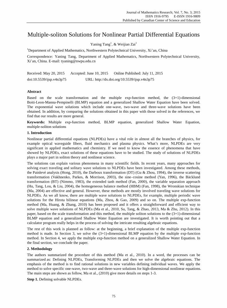
We have plotted the one-wave solution with 0 1a ,

0 2b , 1 2b ,

1 1k , 1 1l ,

1 1m , 1z and

1t , in Figure 1.

www.ccsenet.org/jmr Journal of Mathematics Research Vol. 7, No. 3; 2015

78

Figure 1. The one-wave solution with0 1a ,

0 2b ,1 2b ,

1 1k ,1 1l ,

1 1m , 1z and 1t .

3.2 Two-wave Solutions

Similarly, we require the linear conditions

,i x i ik , ,i y i il ,

,i z i im , ,i t i i , 1 2i , (16)

whereik ,

il ,im and

i , 1 2i , are constants. Based on the Eq. (3), we can obtain the exponential function

solutions

i i i ik x l y m z t

i ic e

, 1 2i . (17)

We then suppose the polynomials,

1 2 1 1 2 2 12 1 2 1 2

1 2 1 1 12 1 1

( , ) 2[ ( ) ],

( , ) 1 ,

p k k a k k

q a

(18)

where 12a are constants to be determined. Substituting Eq. (17) and Eq. (18) into Eq. (4), we obtain the equation

1 2 1 2

1 2 1 2

1 1 2 2 12 1 2 1 2

1 2 12 1 2

2[ ( ) ]( , , , ) ,

1

, 1,2.i i i i i

k c e k c e a k k c e c eu x y z t

c e c e a c e c e

k x l y m z t i

(19)

By the multiple exp-function method and the Eq. (16), we can get the following solutions

1 2 1 1 2 212

1 2 1 1 2 2

3

( )( ),

( )( )

, 1 2.i i

k k m l l ma

k k m l l m

k i

(20)

whereik ,

il andim ,1 2i , are constants. Substituting Eq. (20) into Eq. (19), we obtain the two-wave solutions

of Eq. (10). By the scale transformation x x , we can obtain the two-wave solutions of Eq. (9).

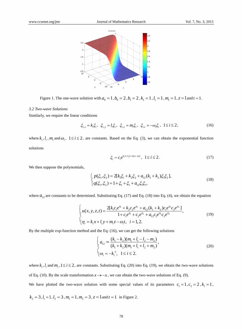
We have plotted the two-wave solution with some special values of its parameters 1 1c ,

2 2c ,1 1k ,

2 3k ,1 1l ,

2 3l ,1 1m ,

2 3m , 1z and 1t in Figure 2.

-10

-5

0

5

10

-10

-5

0

5

100.5

1

1.5

2

2.5

x

z=1,t=1

y

0.6

0.8

1

1.2

1.4

1.6

1.8

2

2.2

2.4

www.ccsenet.org/jmr Journal of Mathematics Research Vol. 7, No. 3; 2015

79

Figure 2. The two-wave solution with1 1c ,

2 2c ,1 1k ,

2 3k ,1 1l ,

2 3l ,1 1m ,

2 3m , 1z and

1t .

3.3 Three-wave Solutions

Again similarly, let’s consider the linear conditions

,i x i ik , ,i y i il ,

,i z i im , ,i t i i

, 1 3i , (21)

whereik ,

il ,im and

i , 1 3i , are constants. Based on the Eq. (3), we can obtain the exponential function

solutions

i i i ik x l y m z t

ii c e

, 1 3i . (22)

In this condition, we set the polynomials as

1 2 3 1 1 2 2 3 3 12 1 2 1 2 13 1 3 1 3

23 2 3 2 3 12 13 23 1 2 3 1 2 3

1 2 3 1 2 3 12 1 2 13 1 3 23 2 3 12 13 23 1 2 3

( , , ) 2[ ( ) ( )

( ) ( ) ],

( , , ) 1 .

p k k k a k k a k k

a k k a a a k k k

q a a a a a a

(23)

where12a ,

13a and23a are constants to be determined. Substituting Eq. (22) and Eq. (23) into Eq. (4), we obtain

the equation

31 2 1 2

3 31 2

31 2 1

1 1 2 2 3 3 12 1 2 1 2

13 1 3 1 3 23 2 3 2 3

12 13 23 1 2 3 1 2 3 1

( , , , ) 2[ ( )

( ) ( )

( ) ] / (1

u x y z t k c e k c e k c e a k k c e c e

a k k c e c e a k k c e c e

a a a k k k c e c e c e c e

3 32 1 2 1

3 32 1 2

2 3 12 1 2 13 1 3

23 2 3 12 13 23 1 2 3

),

, 1, 2,3. i i i i i

c e c e a c e c e a c e c e

a c e c e a a a c e c e c e

k x l y m z t i

(24)

Solving the above polynomials with Eq. (21), we obtain the following relations for the algebraic equations.

3

( )( ),

( )( )

,

i j i j i j

i j i j i j

i i

ij

k k l l m m

k k l l m m

k

a

1 3i ，1 3j ， (25)

-10

-5

0

5

10

-10

-5

0

5

100

2

4

6

8

x

z=1,t=1

y

1

2

3

4

5

6

7

www.ccsenet.org/jmr Journal of Mathematics Research Vol. 7, No. 3; 2015

80

where ik ,

il and im , 1 3i , are constants. Substituting Eq. (25) into Eq. (24), we can get the three-wave

solutions for Eq. (10). By the scale transformation x x , we solve the solutions to Eq. (9). The determination

of three-wave solutions confirms the fact that N -wave solutions exist for any order. The higher level wave

solutions, for 4N , can be obtained in a parallel manner and do not contain any new free parameters other than

ija derived for the three-wave solutions.

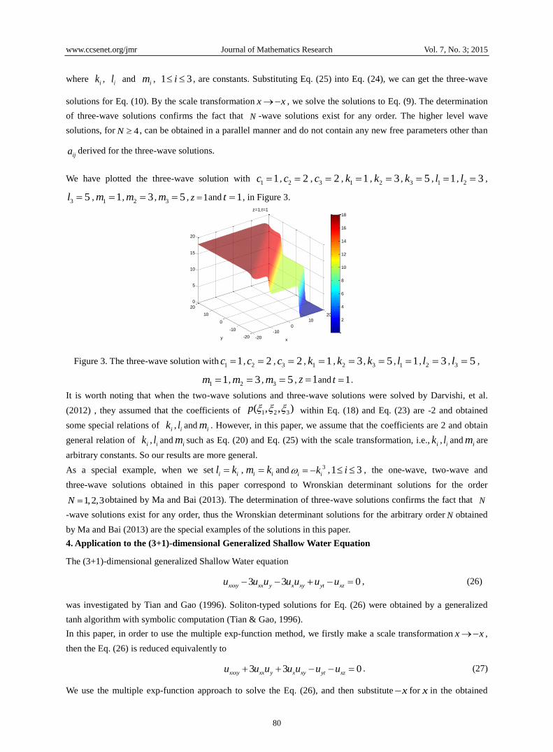
We have plotted the three-wave solution with 1 1c ,

2 2c ,3 2c ,

1 1k ,2 3k ,

3 5k ,1 1l ,

2 3l ,

3 5l ,1 1m ,

2 3m ,3 5m , 1z and 1t , in Figure 3.

Figure 3. The three-wave solution with1 1c ,

2 2c ,3 2c ,

1 1k ,2 3k ,

3 5k ,1 1l ,

2 3l ,3 5l ,

1 1m ,2 3m ,

3 5m , 1z and 1t .

It is worth noting that when the two-wave solutions and three-wave solutions were solved by Darvishi, et al.

(2012) , they assumed that the coefficients of 1 2 3( , , )p within Eq. (18) and Eq. (23) are -2 and obtained

some special relations of ik ,

il andim . However, in this paper, we assume that the coefficients are 2 and obtain

general relation of ik ,

il andim such as Eq. (20) and Eq. (25) with the scale transformation, i.e.,

ik ,il and

im are

arbitrary constants. So our results are more general.

As a special example, when we seti il k ,

i im k and 3

i ik ,1 3i , the one-wave, two-wave and

three-wave solutions obtained in this paper correspond to Wronskian determinant solutions for the order

1,2,3N obtained by Ma and Bai (2013). The determination of three-wave solutions confirms the fact that N

-wave solutions exist for any order, thus the Wronskian determinant solutions for the arbitrary order N obtained

by Ma and Bai (2013) are the special examples of the solutions in this paper.

4. Application to the (3+1)-dimensional Generalized Shallow Water Equation

The (3+1)-dimensional generalized Shallow Water equation

3 3 0xxxy xx y x xy yt xzu u u u u u u , (26)

was investigated by Tian and Gao (1996). Soliton-typed solutions for Eq. (26) were obtained by a generalized

tanh algorithm with symbolic computation (Tian & Gao, 1996).

In this paper, in order to use the multiple exp-function method, we firstly make a scale transformation x x ,

then the Eq. (26) is reduced equivalently to

3 3 0xxxy xx y x xy yt xzu u u u u u u .

(27)

We use the multiple exp-function approach to solve the Eq. (26), and then substitute x for x in the obtained

-20

-10

0

10

20

-20

-10

0

10

20

0

5

10

15

20

x

z=1,t=1

y

2

4

6

8

10

12

14

16

18

www.ccsenet.org/jmr Journal of Mathematics Research Vol. 7, No. 3; 2015

81

solutions. The new solutions have checked in Eq. (26) and all solutions satisfy in the equation. Next, we will

solve one-wave, two-wave and three-wave solutions for Eq. (26).

4.1 One-wave Solutions

By using the approach and the Eq. (11) as well as BLMP equation, we obtain that

2

1 0 1 0 1 1 1 11 1

0 1

(2 ) ( ),

b b k a k m k la

b l

, (28)

where0a ,

0b ,1b ,

1k ,1l and

1m are constants. Substituting Eq. (28) into Eq. (14), we obtain the one-wave

solutions of Eq. (27). By the scale transformation x x , we can obtain the one-wave solutions of Eq. (26).

We have plotted the above result for 0 1a ,

0 1b ,1 1b ,

1 1k ,1 1l ,

1 2m , 1z and 0t , as shown in

Figure 4.

Figure 4. The one-wave solution with 0 1a ,

0 1b ,1 1b ,

1 1k ,1 1l ,

1 2m , 1z and 0t .

4.2 Two-wave Solutions

Similarly, by applying the method and Eq. (16) as well as BLMP equation, we get that

2 2 2 2 2 2 2 2 2

1 2 2 1 1 1 2 2 1 2 1 2 1 2 2 1 1 2 2 1 1 2 1

2 2 2 2 2 2 2

1 1 2 2 2 2 1 1 2 2 1 1 1 2 2 1 2 1 2 1 2 2 1

2 2 2 2

1 2 2 1 1 2 1 1 1 2 2 2 2 1

1 11

12 ( 3 3 3 3

) / (3 3 3

3 ),

(

k k l l k l k l k k l l l l m k k k l l k l m

m l l k m k l k k l l k l k l k k l l l l m k

k k l l k l m m l l k m k l

k k

a

2 2

1 1 2 2 2 22

1 2

) ( ), .

l m k k l m

l l

(29)

whereik ,

il andim , 1 2i , are constants. Substituting Eq. (29) into Eq. (19), we obtain the two-wave solutions

of Eq. (27). By the scale transformation x x , we can obtain the two-wave solutions of Eq. (26).

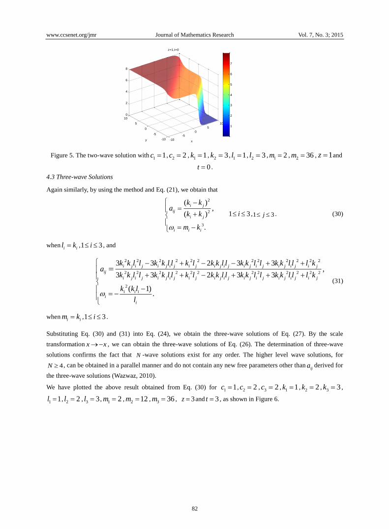
We have plotted the above result for 1 1c ,

2 2c ,1 1k ,

2 3k ,1 1l ,

2 3l ,1 2m ,

2 36m , 1z and

0t , as shown in Figure 5.

-10

-5

0

5

10

-10

-5

0

5

101

1.5

2

2.5

3

x

z=1,t=0

y

1.2

1.4

1.6

1.8

2

2.2

2.4

2.6

2.8

www.ccsenet.org/jmr Journal of Mathematics Research Vol. 7, No. 3; 2015

82

Figure 5. The two-wave solution with1 1c ,

2 2c ,1 1k ,

2 3k ,1 1l ,

2 3l ,1 2m ,

2 36m , 1z and

0t .

4.3 Three-wave Solutions

Again similarly, by using the method and Eq. (21), we obtain that

2

2

3

( ),

( )

.

i j

ij

i j

i i i

k ka

k k

m k

1 3i ,1 3j . (30)

wheni il k ,1 3i , and

2 2 2 2 2 2 2 2 2 2 2 2

2 2 2 2 2 2 2 2 2 2 2 2

2

3 3 2 3 3,

3 3 2 3 3

( 1).

i j i j i j i j i j i j i j i j i j i j i j i j

ij

i j i j i j i j i j i j i j i j i j i j i j i j

i i ii

i

k k l l k k l l k l k k l l k k l l k k l l l ka

k k l l k k l l k l k k l l k k l l k k l l l k

k k l

l

(31)

wheni im k ,1 3i .

Substituting Eq. (30) and (31) into Eq. (24), we obtain the three-wave solutions of Eq. (27). By the scale

transformation x x , we can obtain the three-wave solutions of Eq. (26). The determination of three-wave

solutions confirms the fact that N -wave solutions exist for any order. The higher level wave solutions, for

4N , can be obtained in a parallel manner and do not contain any new free parameters other thanija derived for

the three-wave solutions (Wazwaz, 2010).

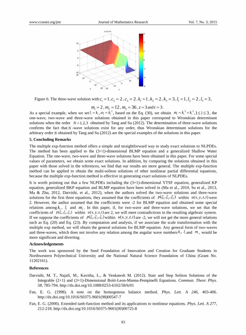
We have plotted the above result obtained from Eq. (30) for 1 1c ,

2 2c ,3 2c ,

1 1k ,2 2k ,

3 3k ,

1 1l ,2 2l ,

3 3l ,1 2m ,

2 12m ,3 36m , 3z and 3t , as shown in Figure 6.

-10

-5

0

5

10

-10

-5

0

5

100

2

4

6

8

x

z=1,t=0

y

1

2

3

4

5

6

7

www.ccsenet.org/jmr Journal of Mathematics Research Vol. 7, No. 3; 2015

83

Figure 6. The three-wave solution with1 1c ,

2 2c ,3 2c ,

1 1k ,2 2k ,

3 3k ,1 1l ,

2 2l ,3 3l ,

1 2m ,2 12m ,

3 36m , 3z and 3t .

As a special example, when we set i il k ,2

i ik , based on the Eq. (30), we obtain 2 3

i i im k k ,1 3i , the

one-wave, two-wave and three-wave solutions obtained in this paper correspond to Wronskian determinant

solutions when the order 1,2,3N obtained by Tang and Su (2012). The determination of three-wave solutions

confirms the fact that N -wave solutions exist for any order, thus Wronskian determinant solutions for the

arbitrary order N obtained by Tang and Su (2012) are the special examples of the solutions in this paper.

5. Concluding Remarks

The multiple exp-function method offers a simple and straightforward way to study exact solutions to NLPDEs.

The method has been applied to the (3+1)-dimensional BLMP equation and a generalized Shallow Water

Equation. The one-wave, two-wave and three-wave solutions have been obtained in this paper. For some special

values of parameters, we obtain some exact solutions. In addition, by comparing the solutions obtained in this

paper with those solved in the references, we find that our results are more general. The multiple exp-function

method can be applied to obtain the multi-soliton solutions of other nonlinear partial differential equations,

because the multiple exp-function method is effective in generating exact solutions of NLPDEs.

It is worth pointing out that a few NLPDEs including the (3+1)-dimensional YTSF equation, generalized KP

equation, generalized BKP equation and BLMP equation have been solved in (Ma et al., 2010, Su et al., 2013,

Ma & Zhu, 2012, Darvishi, et al., 2012), when the authors solved the two-wave solutions and three-wave

solutions for the first three equations, they assumed that the coefficients of 1 2 3( , , )p within ( , , , )u x y z t were

2. However, the author assumed that the coefficients were -2 for BLMP equation and obtained some special

relations amongik ,

il and im . In this paper, if, for two-wave and three-wave solutions, we set that the

coefficients of 1 2 3( , , )p within ( , , , )u x y z t are 2, we will meet contradictions in the resulting algebraic system.

If we suppose the coefficients of 1 2 3( , , )p within ( , , , )u x y z t are -2, we will not get the more general relations

such as Eq. (20) and Eq. (23). By computation and analysis, if we associate the scale transformation with the

multiple exp method, we will obtain the general solutions for BLMP equation. Any general form of two-waves

and three-waves, which does not involve any relation among the angular wave numbers , i ik l and im , would be

more significant and diverting.

Acknowledgements

The work was sponsored by the Seed Foundation of Innovation and Creation for Graduate Students in

Northwestern Polytechnical University and the National Natural Science Foundation of China (Grant No.

11202161).

References

Darvishi, M. T., Najafi, M., Kavitha, L., & Venkatesh M. (2012). Stair and Step Soliton Solutions of the

Integrable (2+1) and (3+1)-Dimensional Boiti-Leon-Manna-Pempinelli Equations. Commun. Theor. Phys.

58, 785-794. http://dx.doi.org/10.1088/0253-6102/58/6/01

Fan, E. G. (1998). A note on the homogenous balance method. Phys. Lett. A 246, 403-406.

http://dx.doi.org/10.1016/S0375-9601(98)00547-7

Fan, E. G. (2000). Extended tanh-function method and its applications to nonlinear equations. Phys. Lett. A 277,

212-218. http://dx.doi.org/10.1016/S0375-9601(00)00725-8

-20

-10

0

10

20

-20

-10

0

10

20

-10

-5

0

5

10

x

z=3,t=3

y -6

-4

-2

0

2

4

6

www.ccsenet.org/jmr Journal of Mathematics Research Vol. 7, No. 3; 2015

84

Gilson, C. R., Nimmo, J. J. C. & Willox R. (1993). A (2+1)-dimensional generalization of the AKNS shallow

water wave equation. Phys. Lett. A 180, 337-345 (1993). http://dx.doi.org/10.1016/0375-9601(93)91187-A

Gu, C. H., & Zhou, Z. X. (1994). On Darboux transformations for soliton equations in high-dimensional

spacetime. Letters in mathematical physics. 32, 1-10. http://dx.doi.org/10.1007/BF00761119

Hong, L. I. (2010). Painlevé analysis and Darboux transformation for a variable-coefficient Boussinesq system

in fluid dynamics with symbolic computation. Commun. Theor. Phys. 53, 831-836. http://dx.doi.org/

10.1088/0253-6102/53/5/08

Hu, H. C., Tang, X. Y., Lou, S. Y., & Liu Q. P. (2004). Variable separation solutions obtained from Darboux

transformations for the asymmetric Nizhnik–Novikov–Veselov system. Chaos Solitons Fract. 22, 327-334.

http://dx.doi.org/10.1016/j.chaos.2004.02.002

Ma, H. C., & Bai, Y. B. (2013). Wronskian Determinant Solutions for the (3+1)-Dimensional

Boiti-Leon-Manna-Pempinelli Equation. Journal of Applied Mathematics and Physics. 1, 18-24.

http://dx.doi.org/10.4236/jamp.2013.15004

Ma, S. H., & Fang, J. P. (2009). Multi dromion-solitoff and fractal excitations for (2+1)-dimensional

Boiti–Leon–Manna–Pempinelli system. Commun. Theor. Phys. 52, 641-645.

http://www.cnki.com.cn/Article/CJFDTotal-CITP200910021.htm

Ma, W. X. (2004). Wronskians, generalized Wronskians and solutions to the Korteweg–de Vries equation. Chaos

Solitons Fract. 19, 163-170. http://dx.doi.org/10.1016/S0960-0779(03)00087-0

Ma, W. X., & Zhu, Z. N. (2012). Solving the (3+1)-dimensional generalized KP and BKP equations by the

multiple exp-function algorithm. Appl. Math. Comput. 218, 11871-11879.

http://dx.doi.org/ 10.1016/j.amc.2012.05.049

Ma, W. X., Huang, T. W., & Zhang, Y. (2010). A multiple exp-function method for nonlinear differential

equations and its application. Phys. Scr. 82, 065003. http://dx.doi.org/10.1088/0031-8949/82/06/065003

Ma, W. X., Zhou, R. G., & Gao, L. (2009). Exact one-periodic and two-periodic wave solutions to Hirota bilinear

equations in (2+1) dimensions. Mod. Phys. Lett. A 24, 1677-1688.

http://dx.doi.org/10.1142/S0217732309030096

Nimmo, J. J. C. (1983). A bilinear Backlund transformation for the nonlinear Schrodinger equation. Phys. Lett. A

99, 279-280. http://dx.doi.org/10.1016/0375-9601(83)90884-8

Su, P. P., Tang, Y. N., & Zhao, Y. (2013). Multiple exp-function Method for Two Kinds of (3+1)-dimensional

Generalized BKP Equations. Chinese Journal of Engineering Mathematics. 30, 890-900.

http://www.cqvip.com/qk/91079x/201306/48091642.html

Tang, Y. N., & Su, P. P. (2012). Two Different Classes of Wronskian Conditions to a (3+1)-Dimensional

Generalized Shallow Water Equations. International Scholarly Research Notices. 2012, 384906.

http://dx.doi.org/10.5402/2012/384906

Tian, B., & Gao, Y. T. (1996). Beyond travelling waves: a new algorithm for solving nonlinear evolution

equations. Comput. Phys. Commun. 95, 139-142. http://dx.doi.org/10.1016/0010-4655(96)00014-8

Vakhnenko, V. O., Parkes, E. J. & Morrison, A. J. (2003). A Bäcklund transformation and the inverse scattering

transform method for the generalised Vakhnenko equation. Chaos Solitons Fract. 17, 683-692.

http://dx.doi.org/10.1016/S0960-0779(02)00483-6

Wazwaz, A. M. (2010). Multiple-Soliton Solutions for Extended Shallow Water Wave Equations. Studies in

Mathematical Sciences. 1, 21–29. http://dx.doi.org/10.3968%2Fj.sms.1923845220120101.003

Yan, C. T. (1996). A simple transformation for nonlinear waves. Phys. Lett. A 224, 77–84 (1996).

http://dx.doi.org/ 10.1016/S0375-9601(96)00770-0

Copyrights

Copyright for this article is retained by the author(s), with first publication rights granted to the journal.

This is an open-access article distributed under the terms and conditions of the Creative Commons Attribution

license (http://creativecommons.org/licenses/by/3.0/).