Multiple Regression Analysis PowerPoint

Multiple Regression Analysis

Example: Housing Prices in Boston CRIM per capita crime rate by town

ZN proportion of residential land zoned for lots over 25,000 ft2

INDUS proportion of non-retail business acres per town

CHASCharles River dummy variable (=1 if tract bounds river; 0 otherwise)

NOX Nitrogen oxide concentration (parts per 10 million)

RM average number of rooms per dwelling

AGE proportion of owner-occupied units built prior to 1940

DIS weighted distances to five Boston employment centres

RAD index of accessibility to radial highways

TAX full-value property-tax rate per $10,000

PTRATIO pupil-teacher ratio by town

B 1000(Bk - 0.63)2 where Bk is the proportion of blacks by town

LSTAT % lower status of the population

MEDV Median value of owner-occupied homes in $1000's

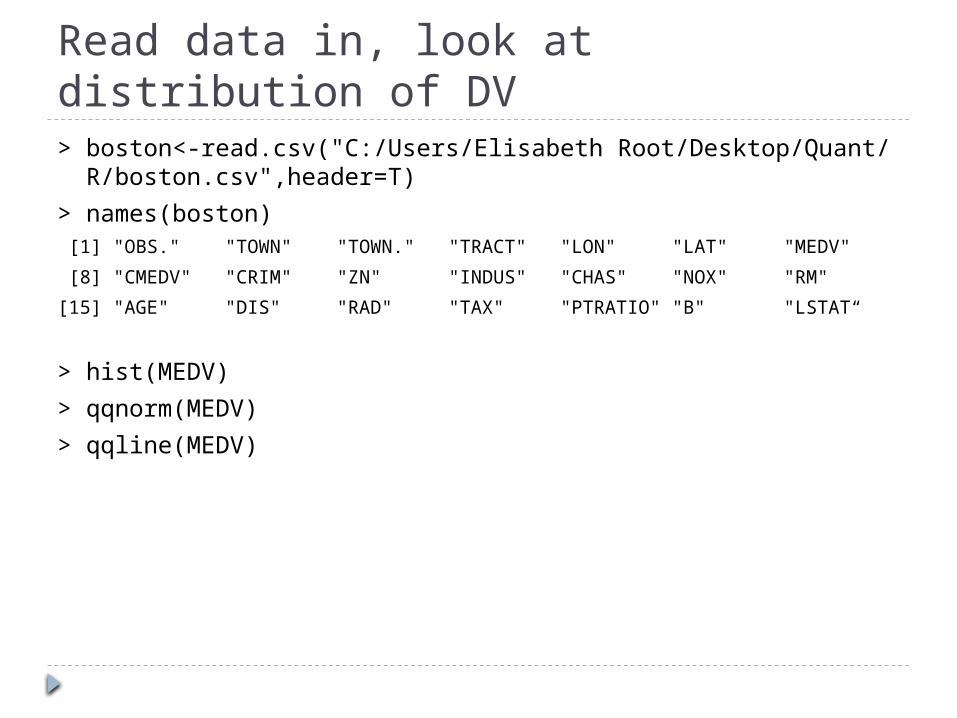
Read data in, look at distribution of DV> boston<-read.csv("C:/Users/Elisabeth Root/Desktop/Quant/ R/boston.csv",header=T)

> names(boston) [1] "OBS." "TOWN" "TOWN." "TRACT" "LON" "LAT" "MEDV"

[8] "CMEDV" "CRIM" "ZN" "INDUS" "CHAS" "NOX" "RM"

[15] "AGE" "DIS" "RAD" "TAX" "PTRATIO" "B" "LSTAT“

> hist(MEDV)> qqnorm(MEDV)> qqline(MEDV)

Histogram and QQPlot

Histogram transformed> boston$LMEDV<-log(boston$MEDV)> hist(LMEDV)

The basic call for linear regression> bost<-lm(LMEDV ~ RM + LSTAT + CRIM + ZN + CHAS + DIS, data=boston)

> summary(bost)

Why do we need data=? Why do we need summary()?

R outputCall:lm(formula = LMEDV ~ RM + LSTAT + CRIM + ZN + CHAS + DIS, data = boston)

Residuals: Min 1Q Median 3Q Max -0.73869 -0.11122 -0.02076 0.10735 0.92643

Coefficients: Estimate Std. Error t value Pr(>|t|) (Intercept) 2.8483185 0.1334153 21.349 < 2e-16 ***RM 0.1177250 0.0175147 6.721 4.93e-11 ***LSTAT -0.0340898 0.0019931 -17.104 < 2e-16 ***CRIM -0.0115538 0.0012645 -9.137 < 2e-16 ***ZN 0.0019266 0.0005587 3.449 0.000611 ***CHAS 0.1349921 0.0375525 3.595 0.000357 ***DIS -0.0294607 0.0067124 -4.389 1.39e-05 ***---Signif. codes: 0 ‘***’ 0.001 ‘**’ 0.01 ‘*’ 0.05 ‘.’ 0.1 ‘ ’ 1

Residual standard error: 0.2109 on 499 degrees of freedomMultiple R-squared: 0.7369, Adjusted R-squared: 0.7337 F-statistic: 232.9 on 6 and 499 DF, p-value: < 2.2e-16

How to use residuals for diagnostics Residual analysis is usually done graphically

using: Quantile plots: to assess normality Histograms and boxplots Scatterplots: to assess model assumptions, such

as constant variance and linearity, and to identify potential outliers

Cook’s D: to check for influential observations

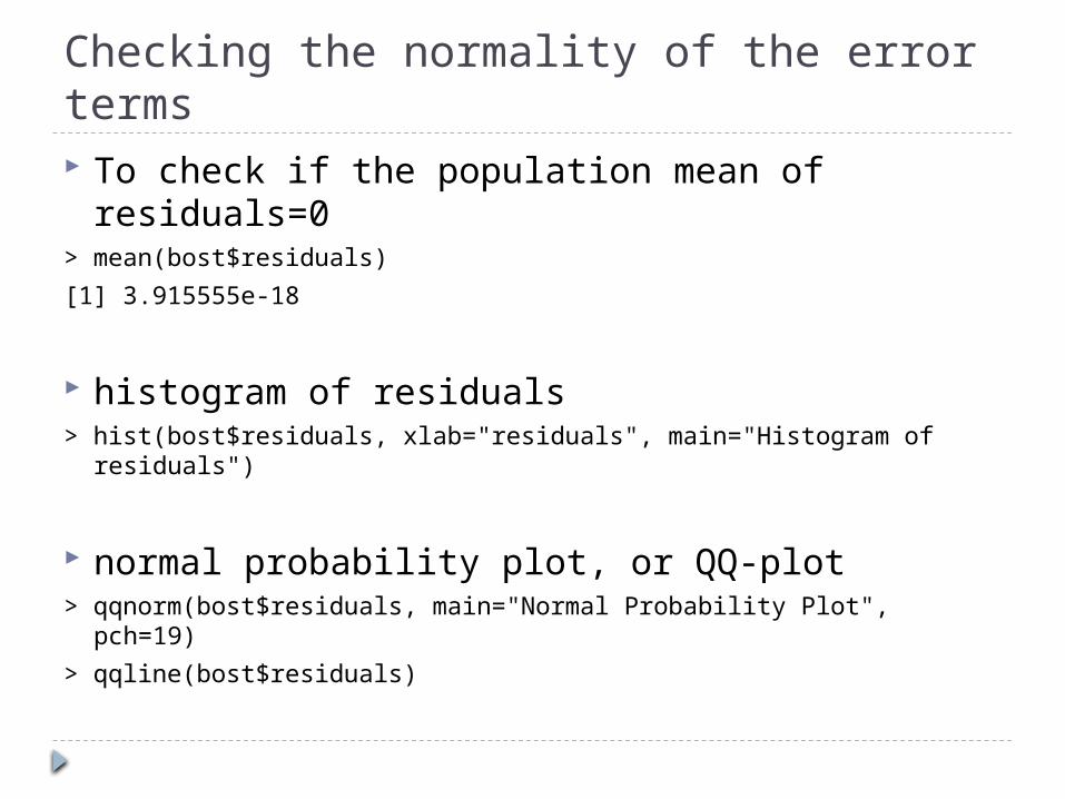
Checking the normality of the error terms To check if the population mean of residuals=0> mean(bost$residuals)[1] 3.915555e-18

histogram of residuals > hist(bost$residuals, xlab="residuals", main="Histogram of

residuals")

  normal probability plot, or QQ-plot> qqnorm(bost$residuals, main="Normal Probability Plot",

pch=19)> qqline(bost$residuals)

Result

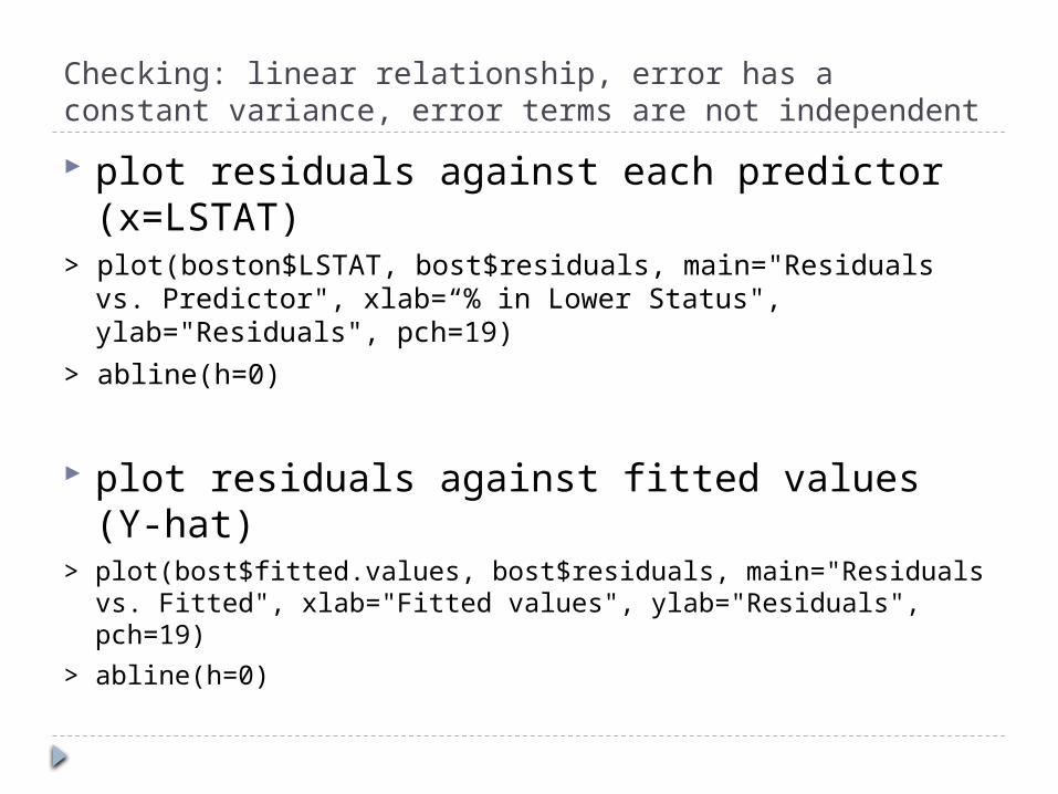
Checking: linear relationship, error has a constant variance, error terms are not independent plot residuals against each predictor

(x=LSTAT)> plot(boston$LSTAT, bost$residuals, main="Residuals vs. Predictor", xlab=“% in Lower Status", ylab="Residuals", pch=19)

> abline(h=0)

  plot residuals against fitted values (Y-hat)> plot(bost$fitted.values, bost$residuals, main="Residuals vs. Fitted", xlab="Fitted values", ylab="Residuals", pch=19)

> abline(h=0)

Result

May need to transform this variable

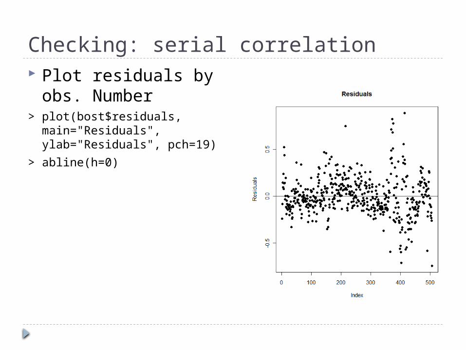
Checking: serial correlation Plot residuals by obs.

Number> plot(bost$residuals, main="Residuals", ylab="Residuals", pch=19)

> abline(h=0)

Checking: influential observations Cook’s D measures the influence of the ith

observation on all n fitted values The magnitude of Di is usually assessed as:

if the percentile value is less than 10 or 20 % than the ith observation has little apparent influence on the fitted values

if the percentile value is greater than 50%, we conclude that the ith observation has significant effect on the fitted values

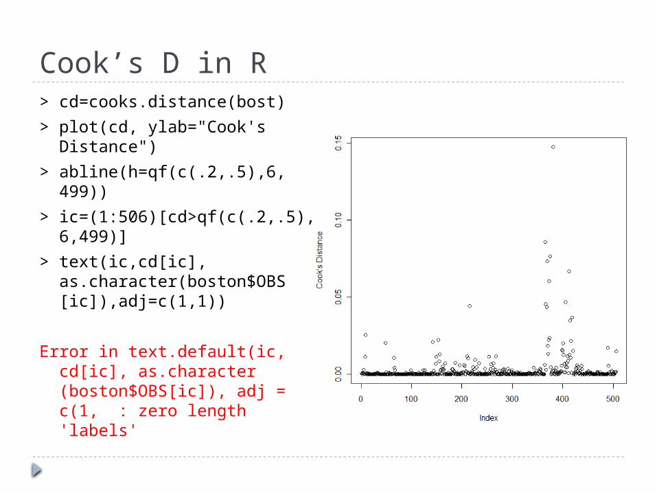
Cook’s D in R> cd=cooks.distance(bost)> plot(cd, ylab="Cook's Distance")

> abline(h=qf(c(.2,.5),6, 499))

> ic=(1:506)[cd>qf(c(.2,.5), 6,499)]

> text(ic,cd[ic], as.character(boston$OBS [ic]),adj=c(1,1))

Error in text.default(ic, cd[ic], as.character (boston$OBS[ic]), adj = c(1, : zero length 'labels'

Stepwise Regression General stepwise regression techniques are

usually a combination of backward elimination and forward selection, alternating between the two techniques at different steps

Typically uses the AIC at each step to select the “next” variable to add

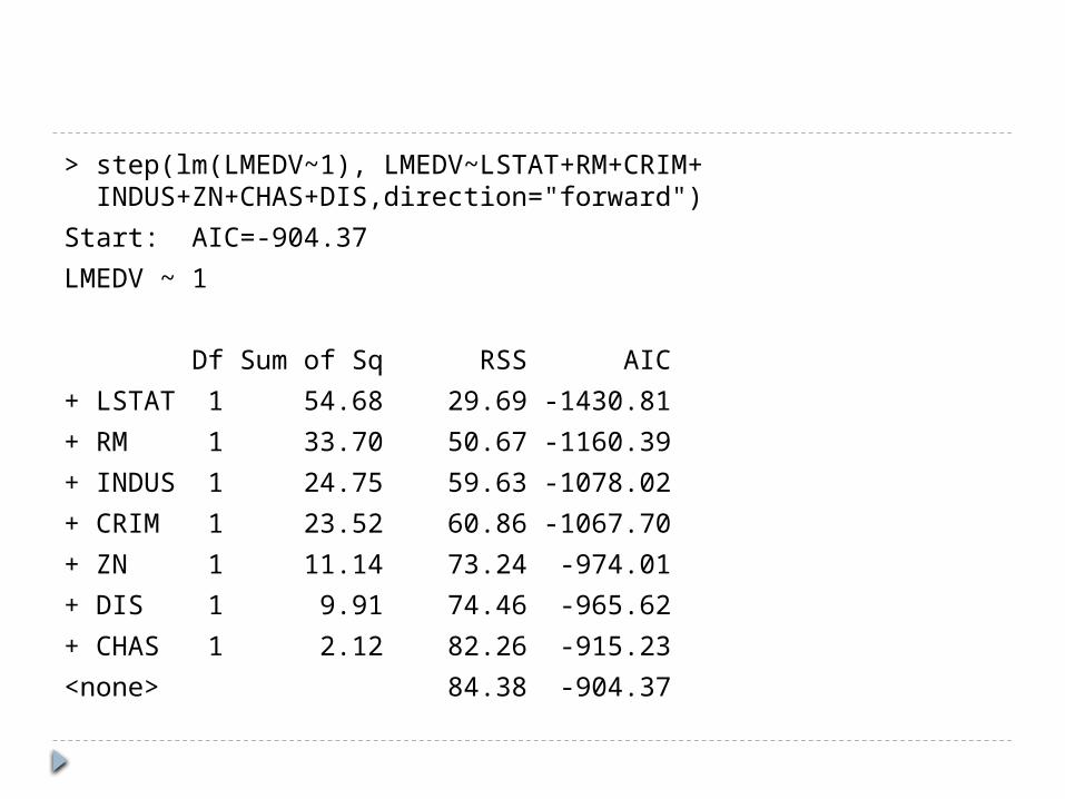
> step(lm(LMEDV~1), LMEDV~LSTAT+RM+CRIM+ INDUS+ZN+CHAS+DIS,direction="forward")

Start: AIC=-904.37LMEDV ~ 1

Df Sum of Sq RSS AIC+ LSTAT 1 54.68 29.69 -1430.81+ RM 1 33.70 50.67 -1160.39+ INDUS 1 24.75 59.63 -1078.02+ CRIM 1 23.52 60.86 -1067.70+ ZN 1 11.14 73.24 -974.01+ DIS 1 9.91 74.46 -965.62+ CHAS 1 2.12 82.26 -915.23<none> 84.38 -904.37

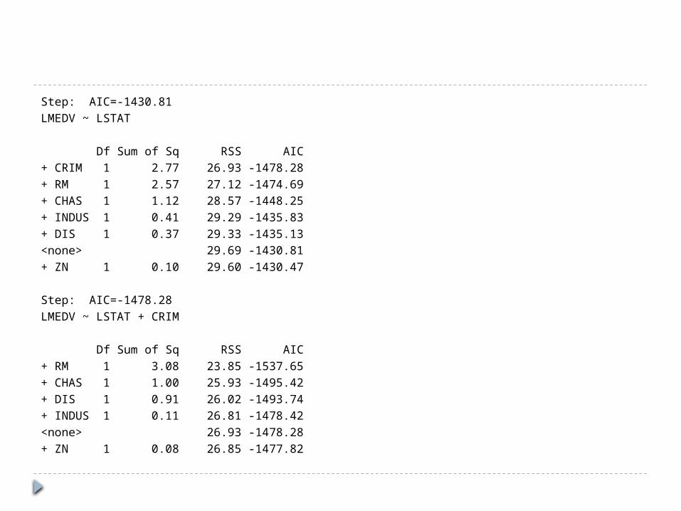
Step: AIC=-1430.81LMEDV ~ LSTAT

Df Sum of Sq RSS AIC+ CRIM 1 2.77 26.93 -1478.28+ RM 1 2.57 27.12 -1474.69+ CHAS 1 1.12 28.57 -1448.25+ INDUS 1 0.41 29.29 -1435.83+ DIS 1 0.37 29.33 -1435.13<none> 29.69 -1430.81+ ZN 1 0.10 29.60 -1430.47

Step: AIC=-1478.28LMEDV ~ LSTAT + CRIM

Df Sum of Sq RSS AIC+ RM 1 3.08 23.85 -1537.65+ CHAS 1 1.00 25.93 -1495.42+ DIS 1 0.91 26.02 -1493.74+ INDUS 1 0.11 26.81 -1478.42<none> 26.93 -1478.28+ ZN 1 0.08 26.85 -1477.82

Step: AIC=-1537.65LMEDV ~ LSTAT + CRIM + RM

Df Sum of Sq RSS AIC+ CHAS 1 0.75 23.10 -1551.86+ DIS 1 0.53 23.32 -1547.11<none> 23.85 -1537.65+ INDUS 1 0.06 23.79 -1536.97+ ZN 1 0.02 23.83 -1536.07

Step: AIC=-1551.86LMEDV ~ LSTAT + CRIM + RM + CHAS

Df Sum of Sq RSS AIC+ DIS 1 0.37 22.73 -1558.08+ INDUS 1 0.14 22.97 -1552.83<none> 23.10 -1551.86+ ZN 1 0.04 23.06 -1550.83

Step: AIC=-1558.08LMEDV ~ LSTAT + CRIM + RM + CHAS + DIS

Df Sum of Sq RSS AIC+ INDUS 1 0.78 21.95 -1573.75+ ZN 1 0.53 22.20 -1568.00<none> 22.73 -1558.08

Step: AIC=-1573.75LMEDV ~ LSTAT + CRIM + RM + CHAS + DIS + INDUS

Df Sum of Sq RSS AIC+ ZN 1 0.46 21.49 -1582.44<none> 21.95 -1573.75

Step: AIC=-1582.44LMEDV ~ LSTAT + CRIM + RM + CHAS + DIS + INDUS + ZN

Model improvement?> bost1<-lm(LMEDV ~ RM + LSTAT + CRIM + ZN + CHAS + DIS)> bost2<-lm(LMEDV ~ RM + LSTAT + CRIM + CHAS + DIS)> anova(bost1,bost2)

Analysis of Variance Table

Model 1: LMEDV ~ RM + LSTAT + CRIM + ZN + CHAS + DISModel 2: LMEDV ~ RM + LSTAT + CRIM + CHAS + DIS Res.Df RSS Df Sum of Sq F Pr(>F) 1 499 22.1993 2 500 22.7284 -1 -0.5291 11.893 0.0006111 ***