Multiple Regression

Multiple Regression

What Techniques Can Tell Us

• Chi Square- • Do groups differ (nominal data)?• T Test• Do Groups/Variables differ?• Gamma/Lambda/Kendall’s Tau etc• Are variables related to each other? (nominal

data)• Correlation• Are variables related to each other?

(ratio/interval data)

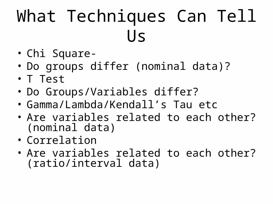
Interpreting Correlations

• 3 questions we can answer

1. Is there a relationship between 2 variables?

2. What is the direction of the relationship?

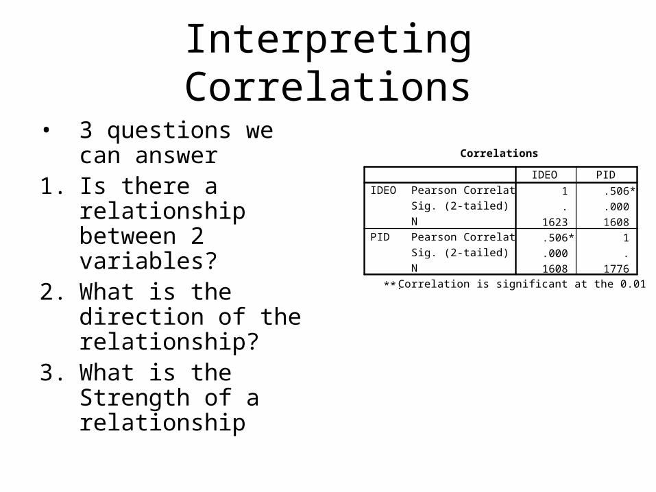
3. What is the Strength of a relationship

Correlations

1 .506**

. .000

1623 1608

.506** 1

.000 .

1608 1776

Pearson Correlation

Sig. (2-tailed)

N

Pearson Correlation

Sig. (2-tailed)

N

IDEO

PID

IDEO PID

Correlation is significant at the 0.01 level(2-tailed).

**.

Interpreting Correlations

• Are there limitations here? And if so, what?

• Don’t know amount of effect of one variable on other

• Don’t know impact of other variables

Correlations

1 .506**

. .000

1623 1608

.506** 1

.000 .

1608 1776

Pearson Correlation

Sig. (2-tailed)

N

Pearson Correlation

Sig. (2-tailed)

N

IDEO

PID

IDEO PID

Correlation is significant at the 0.01 level(2-tailed).

**.

VAR00002

3020100

VA

R8

80

60

40

20

0

-20

-40

-60

RND2

403020100-10-20-30-40

RN

D1

40

30

20

10

0

-10

-20

-30

-40

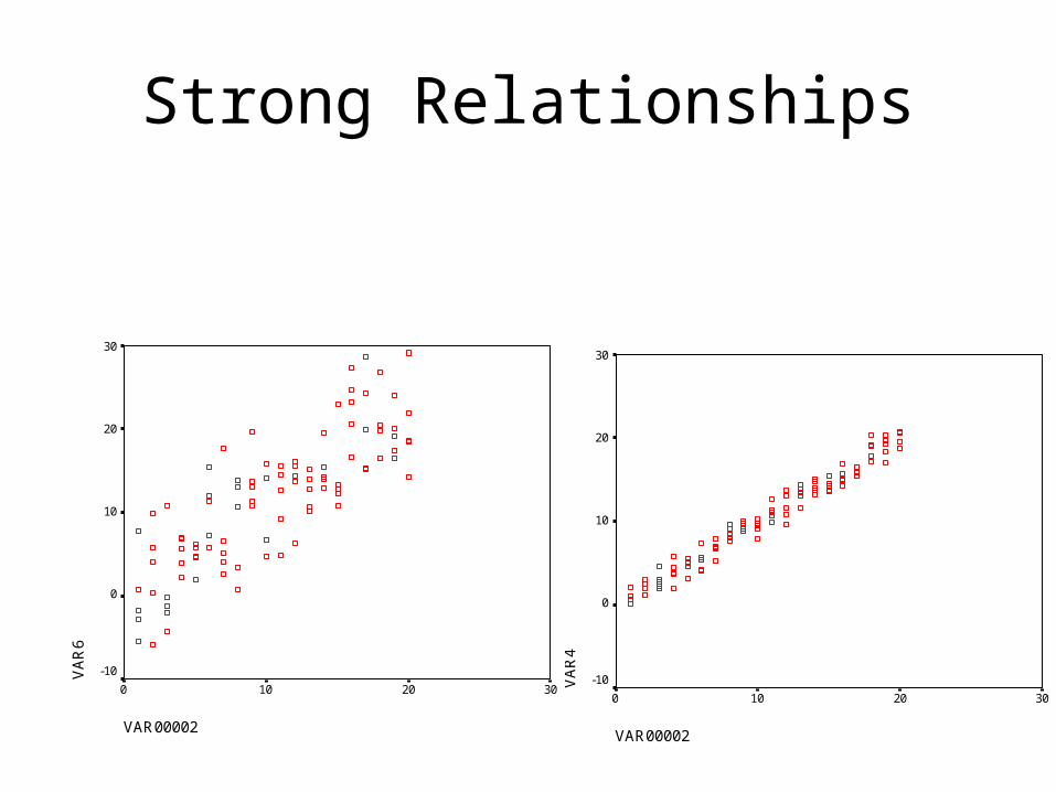
Strength

VAR00002

3020100

VA

R4

30

20

10

0

-10

VAR00002

3020100

VA

R6

30

20

10

0

-10

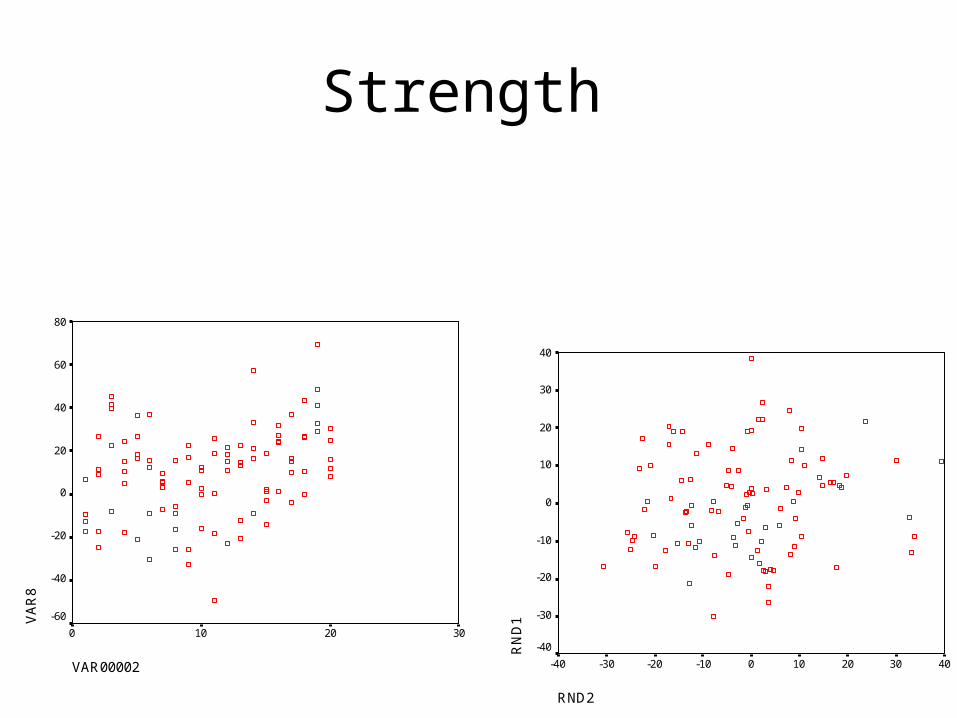
Strong Relationships

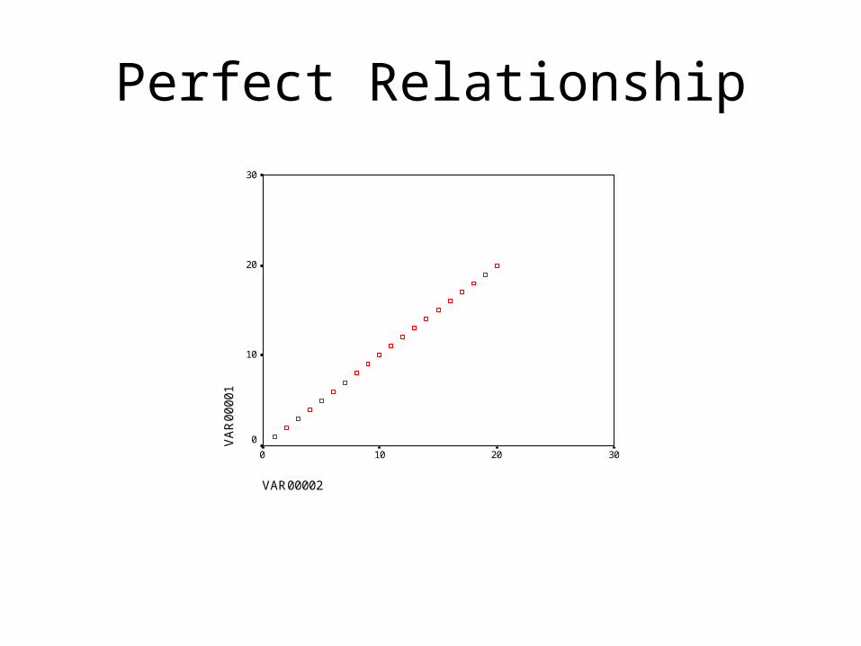
Perfect Relationship

VAR00002

3020100

VA

R0

00

01

30

20

10

0

Basic Equations

• Let your DV (Y)= total cost of bananas• Suppose you buy X lbs of bananas at $.49 a lb• How would you express this as an equation to

figure out how much your bananas are worth?• Y=.49 X• Can use for prediction• 10lbs=$4.90• 2lbs=$.98

Multivariate Equations

• Suppose you have a phone plan that charges – $5.95 a month– $.10 a minute instate long distance– $.08 a minute interstate long distance– $.01 a minute Local Calls

• How would you represent?

• Total=.1x1+.08x2+.01x3+5.95

Regression Analysis

• Lets you work the problem Backwards

• How much do different IVs contribute to a DV

• How do different IVs relate to DV

• Lets you build a model of more complicated relationships

• In addition to existence, direction, strength, gives you the amount of change

Expressing A regression equation

• Y=b1x1+b2x2+…..bixi+constant+error

• Error is part of probabilistic nature of social science

• Constant- what Y would equal if all Xs=0

• Estimation process- fit a line to data that minimizes the distance to all observed data points

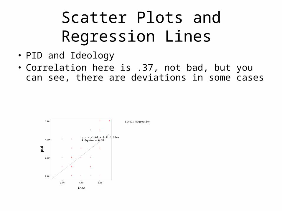
Scatter Plots and Regression Lines

• PID and Ideology • Correlation here is .37, not bad, but you can see,

there are deviations in some cases

Linear Regression

2.00 4.00 6.00

ideo

0.00

2.00

4.00

6.00

pid

pid = -1.05 + 0.81 * ideoR-Square = 0.37

Fitting the Regression Line

• Goal: Minimize the squared distances (error) between predicted values of Y and observed values.

• Goal, explain the variance in Y in terms of X

• Error in prediction is unexplained variance

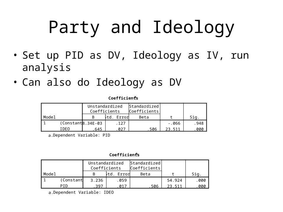
Party and Ideology

• Set up PID as DV, Ideology as IV, run analysis• Can also do Ideology as DV

Coefficientsa

-8.34E-03 .127 -.066 .948

.645 .027 .506 23.511 .000

(Constant)

IDEO

Model1

B Std. Error

UnstandardizedCoefficients

Beta

StandardizedCoefficients

t Sig.

Dependent Variable: PIDa.

Coefficientsa

3.236 .059 54.924 .000

.397 .017 .506 23.511 .000

(Constant)

PID

Model1

B Std. Error


Beta


t Sig.

Dependent Variable: IDEOa.

Goodness of Fit

• Measure of how much variance is explained by model you build

• R2= correlation coefficient squared • R2= proportion of variance explained• R2 is symetrical• In previous example R2 = .256• R2 ranges from 0-1• Adjusted R2 takes into account the degrees of

freedom, more appropriate measure

Run for the Border Using Multiple Regression

• Suppose that you and some friends ate at Taco bell every week for a year.

• For each meal, you know the total amount spent, and the number of each item, but not what each item cost.

• You could use multiple regression to get parameter estimates of the true values.

• Data set was constructed by choosing a random number (Between 0 and 4) of Bean Burritos, Tacos, Chalupas, Chicken Tacos, Beef Burritos, 7 Layer Burritos, and Soft drinks

• Data matrix includes a variable for number of each

Border Model 1

• We’ll look at impact of bean burritos on total

Model Summaryb

.039a .002 -.018 3.74743Model1

R R SquareAdjustedR Square

Std. Error ofthe Estimate

Predictors: (Constant), BEANBURa.

Dependent Variable: TOTAL2b.

Coefficientsa

21.561 1.165 18.507 .000

-.131 .476 -.039 -.276 .784 1.000 1.000

(Constant)

BEANBUR

Model1

B Std. Error


Beta


t Sig. Tolerance VIF

Collinearity Statistics

Dependent Variable: TOTAL2a.

Border Model 2

• Bean Burritos and Tacos

Model Summaryb

.257a .066 .028 3.66072Model1



Predictors: (Constant), TACO, BEANBURa.


Coefficientsa

19.655 1.538 12.781 .000

-.185 .466 -.055 -.397 .693 .996 1.004

.842 .457 .255 1.843 .071 .996 1.004

(Constant)

BEANBUR

TACO

Model1

B Std. Error


Beta





Border Model 3Model Summaryb

.298a .089 .032 3.65375Model1



Predictors: (Constant), CHICKTAC, BEANBUR, TACOa.


Coefficientsa

18.032 2.139 8.432 .000

-.160 .465 -.047 -.343 .733 .994 1.006

.891 .458 .270 1.945 .058 .986 1.014

.554 .508 .151 1.090 .281 .987 1.013

(Constant)

BEANBUR

TACO

CHICKTAC

Model1

B Std. Error


Beta





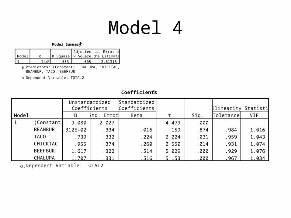
Model 4Model Summaryb

.744a .553 .505 2.61316Model1



Predictors: (Constant), CHALUPA, CHICKTAC,BEANBUR, TACO, BEEFBUR

a.


Coefficientsa

9.080 2.027 4.479 .000

5.312E-02 .334 .016 .159 .874 .984 1.016

.739 .332 .224 2.224 .031 .959 1.043

.955 .374 .260 2.550 .014 .931 1.074

1.617 .322 .514 5.029 .000 .929 1.076

1.707 .331 .516 5.153 .000 .967 1.034

(Constant)

BEANBUR

TACO

CHICKTAC

BEEFBUR

CHALUPA

Model1

B Std. Error


Beta





Linear Regression

16.00 20.00 24.00 28.00

total2

16.00000

20.00000

24.00000

28.00000U

nst

and

ard

ized

Pre

dic

ted

Val

ue

Unstandardized Predicted Value = 9.50 + 0.55 * total2R-Square = 0.55

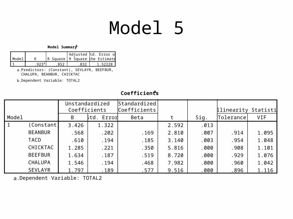
Model 5Model Summaryb

.923a .852 .832 1.52228Model1



Predictors: (Constant), SEVLAYR, BEEFBUR, TACO,CHALUPA, BEANBUR, CHICKTAC

a.


Coefficientsa

3.426 1.322 2.592 .013

.568 .202 .169 2.810 .007 .914 1.095

.610 .194 .185 3.140 .003 .954 1.048

1.285 .221 .350 5.816 .000 .908 1.101

1.634 .187 .519 8.720 .000 .929 1.076

1.546 .194 .468 7.982 .000 .960 1.042

1.797 .189 .577 9.516 .000 .896 1.116

(Constant)

BEANBUR

TACO

CHICKTAC

BEEFBUR

CHALUPA

SEVLAYR

Model1

B Std. Error


Beta





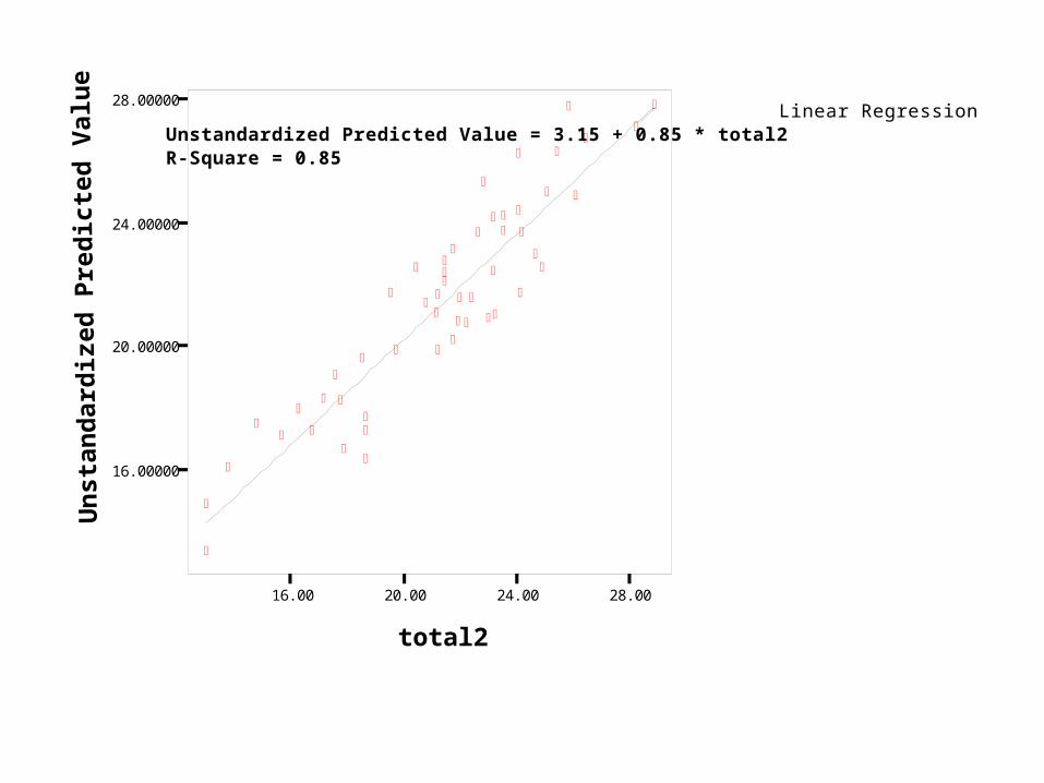
Linear Regression

16.00 20.00 24.00 28.00

total2

16.00000

20.00000

24.00000

28.00000U

nst

and

ard

ized

Pre

dic

ted

Val

ue


Full ModelModel Summaryb

1.000a 1.000 1.000 .00000Model1



Predictors: (Constant), DRINK, SEVLAYR, BEEFBUR,TACO, BEANBUR, CHICKTAC, CHALUPA

a.


Coefficientsa

2.269E-15 .000 . .

.690 .000 .205 . . .906 1.104

.790 .000 .239 . . .936 1.069

1.390 .000 .379 . . .904 1.107

1.590 .000 .505 . . .928 1.078

1.190 .000 .360 . . .893 1.120

1.890 .000 .607 . . .891 1.122

1.290 .000 .404 . . .909 1.100

(Constant)

BEANBUR

TACO

CHICKTAC

BEEFBUR

CHALUPA

SEVLAYR

DRINK

Model1

B Std. Error


Beta





Linear Regression

16.00 20.00 24.00 28.00

total2

16.00000

20.00000

24.00000

28.00000

Un

stan

dar

diz

ed P

red

icte

d V

alu

e


Model 4 Revisited

• Bean Burrito- .69,Taco .79, Chalupa 1.19, Chicken taco 1.39, Beef Burrito 1.59,7 layer 1.89, Drink 1.29

Coefficientsa

9.080 2.027 4.479 .000

5.312E-02 .334 .016 .159 .874 .984 1.016

.739 .332 .224 2.224 .031 .959 1.043

.955 .374 .260 2.550 .014 .931 1.074

1.617 .322 .514 5.029 .000 .929 1.076

1.707 .331 .516 5.153 .000 .967 1.034

(Constant)

BEANBUR

TACO

CHICKTAC

BEEFBUR

CHALUPA

Model1

B Std. Error


Beta





Some Data Requirements for Regression

• DV must be interval or ratio, and continuous

• IVs should not be correlated with each other

• Error should be constant at high and low predicted value (homoschedasticity)

• Relationship must be linear• Errors of subsequent observations should

not be correlated (no serial correlation)

For Next time

• Multicolinearity

• Heteroskedasticity

• Interaction terms

• Pass out Stat Assignment II

Multiple Regression

Documents

totalborder model

tacosborder model

number of eachborder

layer burritos

beef burritos

impact of bean burritos

predicted values of

regression analysislets