Multiple Objective Spanning Trees ... - Optimization Online · where the optimization of several problems is based on spanning trees, factors like the maintenance and communication

1

MOST – Multiple Objective Spanning TreesRepository Project♣

(Technical Report)

Pedro Cardoso♠ and Mario Jesus♥ and Alberto Marquez♦

Abstract

This article presents the Multiple Objective Spanning Trees repository – MOST –Project. As the name suggests, the MOST Project intends to maintain a repositoryof tests for the MOST related problems, mainly addressing real-life situations.

MOST is motivated by the scarcity of repositories for the problems in the referredfield. This entails difficulty in test and classify the proposed algorithms based ontheir performance.

At present, the problems are expressed as networks classified according to their in-trinsic properties, namely nodes, edges, and weights. Different generators were de-veloped, which upon combinations, allow a large number of problems with distinctfeatures like, large sets of solutions, concave fronts, and fronts with gaps.

This repository is open to the general participation of the interested communities,mainly in terms of original contributions, approximation improvements, and prob-lem variations (besides the unconstrained cases).

MOST Project can be found at http://est.ualg.pt/adec/csc/most.

Keywords:Multiobjective optimization, minimum cost spanningtree, libraries.

∗♣ – The authors thank the Centro de Simulacao e Calculo (CsC) from Department of Civil Engineering, EST,University of Algarve, for the computational resources made available.♠ – Department of Electrical EngineeringEST, University of Algarve, Faro, [email protected]♥ – Department of Civil EngineeringEST, University of Algarve, Faro, [email protected]♦ – Department of Applied Math IUniversity of Seville, Seville, Spain [email protected]

1 Introduction

The use of heuristics and meta-heuristics in optimization requires thatthose methods are tested with known problems and solutions to pre-dict their overall performance. The use of large sets of problems reducesthe risk of overfitting in the tested methods although, even in an exten-sive collection, some classes of features may be rare or absent (Gent andWalsh, 1999; Deb et al., 2002).

When we try to focus on some specific problem often a number ofdifficulties arise, like, the need to find repositories for the problems incontext (or possibly similar), the need to know the optimums or quasi-optimums of the problems and, in the majority of the cases, the lack ofdiversity of the so far studied instances. This situation implies that gen-erally the proposed algorithms are first tested with classical problems,as for example, some libraries of functions for the continuous cases, orthe travelling salesman problem for the discrete ones. This proves tobe a touchstone to many meta-heuristics (Johnson and McGeoch, 1997;Cirasella et al., 2001).

It should be noted that this lack of choices is even more pertinent inthe multiple objective combinatorial optimization, where only a few dis-perse sets of results are available. Therefore, in this article we proposethe Multiple Objective Spanning Tree repository – MOST – Project. Thisproject will serve as an archive for the large number of multidisciplinaryapplications problems of the multiple objective spanning trees. The ob-jective of the MOST Project is to establish, maintain, and successivelyimprove an intuitive and large set of problems along with their optimalor quasi-optimal solutions, on which different algorithms can quickly betested and classified relative to their performance, with respect to pro-cessing time and accuracy.

Therefore, MOST Project is meant to be a dynamic platform that theinterested community can make use of and contribute as well to main-tain a helpful repository for the types of problems already mentioned.MOST can be accessed via Internet at http://est.ualg.pt/adec/csc/most.

Relative to the groundwork of the MOST Project, the spanning treesoptimization problem is one of the most well-studied areas in the combi-natorial optimization, with practical applications in distinct areas like,VLSI layout, electricity, water, telecommunication or traffic networks(Sack and Urrutia, 2000), biology and medicine (such as cancer detection– medical imaging(An et al., 2000)), dependency parsing (Hajic et al.,

2

2005), and also as a basic step in some other graph problems.

In the multiple objective minimum spanning tree problems, similarto the generalized multiple objective optimization cases, improving oneof the weights of a good solution will worsen at least one of the others,which implies that there rarely exists an over performing response thatis preferable to all others. Therefore, the answer to these problems isa set of trade-off compromises between all concurring weights, result-ing in a set of solutions. For example, in a telecommunication network,where the optimization of several problems is based on spanning trees,factors like the maintenance and communication costs, communicationdelays, reliability, bandwidth, and profitability, compete among them-selves (Pinto et al., 2005). This intricacy implies that the multiple objec-tive minimum spanning trees problem is NP -complete (Camerini et al.,1984), and Hamacher and Ruhe proved that it is also NP −#(Hamacherand Ruhe, 1994).

Problems in NP -hard class of complexity have attracted for the at-tention of several researchers in that they used ever-increasing compu-tational capacities to shape and develop a large number of heuristicsand meta-heuristics, like the Genetic Algorithms (Vose, 1999; Aarts andLenstra, 1997; Deb, 2001), Tabu Search (Glover and Laguna, 1997), Simu-lated Annealing (Kirkpatrick et al., 1983), and Ant Colony Optimization(Dorigo et al., 1999; Dorigo and Stutzle, 2004). These methods proved tobe excellent working tools and are being adopted as first-choice proce-dures to obtain suitable approximations to many solutions of problems.Although some of these algorithms have the guaranty of convergencethrough the optimum solutions (see for example (Dorigo and Stutzle,2004) for the Ant Colony Optimization or (Coello-Coello et al., 2005) forthe Simulated Annealing, an Artificial Immune System and a GeneralEvolutionary Algorithm for multiple objective optimization problems),most of the times they cannot exactly predict the quality of the approx-imations computed within a limited time. Therefore, if with these tech-niques we look for an extensive problem solver, then we should at leasttest them in greatest possible number of different problems, to estimatetheir performance in several effective measures and rank the algorithms’utility as practical tools. This has been mentioned in the beginning of thearticle: it is exactly here that the MOST Project has to prove its usefulnessby providing a variety of problems and their exact solutions or knowngood approximations.

In the present implementation stage of MOST Project, problems are

3

classified according to three types of generators: nodes, edges, andweights generators. For each of the types, we have defined a set of in-stances, as follows:

• For the nodes we consider five generators: the Grid Nodes Genera-tor, the Triangular Nodes Generator, the Uniform Nodes Generator,the Normal Nodes Generators, and the Clusters Nodes Generator.

• For the edges, six generators are considered: the Grid Edges Gener-ator, the Delaunay Edges Generator, the k-Convex Edges Generator,the Complete Edges Generator, the Voronoi Edges Generator, andthe Clusters Edges Generator.

• Finally, for the edge weights, we consider three generators: the Ran-dom Weights Generator, the ρ-Correlated Weights Generator, andthe Concave Weights Generator.

Therefore, this article is organized as follows. In the next section,some preliminary concepts about multiple objective optimization andnetworks are introduced. Section 3 describes the methods to generatethe networks, namely: the nodes, the edges, and the weights generators.In sections 4 and 5, we suggest the use of three reference metrics anddiscuss the methods used to compute the approximations (in small in-stances the exact solutions). Some examples along with conclusions andfuture work are presented in the last sections.

2 Preliminaries

Mathematically, a multiple objective or criteria optimization problem canbe stated as

mins∈SW(s), (1)

where S is the feasible set and

W : S → IRm

s 7→ W(s) = (w1(s), w2(s), . . . , wm(s))(2)

is them-objective (vector) function, for which all objectives are to be min-imized. Note that if some of the objectives was to be maximized, wecould use the dual principle and therefore still use (1) (Deb, 2001).

The optimization process requires the definition of an order relation.The prevailing relation, in the multiple objective optimization area, is de-fined as follows: in a minimization process, a vector x = (x1, x2, . . . , xm)

4

is said to dominate a vector y = (y1, y2, . . . , ym), and we write x ≺ y, ifxi ≤ yi for all i ∈ {1, 2, . . . ,m}, and for at least one j ∈ {1, 2, . . . ,m} wehave xj < yj . A solution is said to be Pareto optimal if it is not dominatedby any other solution of the feasible set. The set of all the Pareto optimalsolutions is called Pareto(-optimal) set or efficient set.

A network is a structure defined as

N = (V , E ,Z) , (3)

where V is the set of nodes or vertices, E is the set of edges and Z : E →IRm is the weight vector function associating to each edge, e ∈ E , valuesZ(e) = (z1(e), z2(e), . . . , zm(e)). Throughout this article, we will considerthat N is undirected.

For a sub-network T of N , it is considered the sum weight functionas

W(T ) = (w1(T ), w2(T ), . . . , wm(T )) =

=

(∑e∈T

z1(e), . . . ,∑e∈T

zm(e)

)= (4)

=∑e∈T

Z(e),

where e ∈ T means that e is an edge that belongs to T .

3 Network Generators

The network-generating process is divided into three phases that we willdescribe in this section. The method starts by generating a set of nodes,followed by the computation of a set of edges. The network constructionis concluded by setting the edges weights. There will be a single ex-ception to this sequence, as we will see in Section 3.2.5, when a Voronoidiagram is used to set up the edges, since the original set of nodes isreplaced by the one induced by the diagram.

3.1 Nodes generators

One of the main objectives of the MOST Project is to start with a num-ber of networks that could reproduce practical problems, as much aspossible. After a previous analysis, we decided to start with five typesof nodes generators, namely: Grid, Triangular, Uniform, Normal, and

5

Cluster Nodes Generator. The first two generators can be classified asregular since they return regular clouds of nodes. The third and forthcases are examples of a generator that uses pseudo-random numbers as-sociated with statistical distributions. In particular, we use the Uniformand Normal distributions. Finally, the previous generators are appliedto create a set of nodes clusters. First, we calculate a set of centers, whichis followed by the generation of a set of nodes located in the neighbor-hood of those centers. Next, we give a detailed description of each oneof these methods.

3.1.1 Grid Nodes Generator (GNG)

The simplest case is that of a Grid Node Generator. The set of nodesproduced here is distributed over an m × n lattice. To simplify the text,GNGm,n will represent an instance of that generator, with m lines and ncolumns of nodes,

V = GNGm,n = {(x, y) : x ∈ {1, 2, . . . , n}, y ∈ {1, 2, . . . ,m}}.

In Figure 1(b) we can see an example of a GNG10,10.

HdL HeL HfL

HaL

l�!!!!!3 l

������������������

2

l

HbL HcL

Figure 1: (a) Height of an equilateral triangle with side l. Graphicalrepresentation of nodes distribution according to the nodes generator:(b)GNG10,10; (c) TNG10,10; (d) UNG1000; (e) NNG1000; and (f) ClNG50,50.

6

3.1.2 Triangular Nodes Generator (TNG)

Like GNG, the Triangle Nodes Generator also sets m lines with n nodesper line, TNGm,n, distributed according to Algorithm 1. In Figure 1(c),we can see the nodes distribution for a TNG10,10.

Algorithm 1 Triangular Nodes Generator

input: m, n, l, h = l√

32

. m, n – Number of lines and number of nodesby line; l – distance between neighbor nodes; h - distance between lines (seeFigure 1(a))

output: V . set of nodes1: V = ∅2: for all (x, y) ∈ {1, 2, ..., n} × {1, 2, ...,m} do3: if x is odd then4: V = V ∪ {(x× l, y × h)}5: else6: V = V ∪ {(x× l + l

2, y × h)}

7: return V

3.1.3 Statistical Nodes Generator

The Statistical Nodes Generator uses (pseudo) random number gener-ators defined by two statistical distributions, ZX and ZY (associated tox and y coordinates, respectively), to yield as much nodes as necessary.Algorithm 2 describes the process, where random(Z) is a function thatreturns a (pseudo) random number with specified distribution Z.

We considered two instances of the Statistical Nodes Generator ob-tained with the Uniform and the Normal distributions.

Uniform Nodes Generator (UNG) As stated, the Uniform Nodes Gen-erator is a particular case of the Statistical Nodes Generator and UNGn

represents an instance of UNG with n nodes. In this case, ZX ∼

Algorithm 2 Statistical Nodes Generatorinput: ZX , ZY , n . ZX , ZY – statistical distributions; n – number of nodesoutput: V . set of nodes

1: V = ∅2: for i = 1, 2, ..., n do3: V = V ∪ {(random(ZX), random(ZY ))}4: return V

7

U [xmin, xmax] and ZY ∼ U [ymin, ymax], where U [a, b] is the Uniform distri-bution over the interval [a, b], and xmin, xmax, ymin, and ymax are generatorparameters. This produces a cloud of nodes uniformly distributed overthe rectangle [xmin, xmax]× [ymin, ymax].

In Figure 1(d) we can see an example of the distribution for n = 1000nodes, UNG1000, with xmin = ymin = 0, and xmax = ymax = 1000.

Normal Nodes Generator (NNG) The Normal Nodes Generator is alsoa particular case of the Statistical Nodes Generator andNNGn representsan instance with n nodes. Here, ZX ∼ N(µX , σX) and ZY ∼ N(µY , σY ),where N(µ, σ) is the Normal distribution with mean µ and standard de-viation σ, and µX , µY , σX and σY are generator parameters.

In this case, the cloud of nodes is distributed around (µX , µY ) withhorizontal and vertical deviations associated with the values of σX andσY , respectively.

In Figure 1(e) we can see the cloud of nodes for NNG1000, with µx =µy = 10000 and σx = σy = 100.

3.1.4 Clusters Nodes Generator (ClNG)

The last nodes generator that we will consider is the Clusters Nodes Gen-erator. The ClNG uses, in two steps, the previous generators, to producea set of m clusters with n nodes each. In the first phase, m nodes aregenerated, c = (cx, cy), around which, in the second phase, the clustersare completed by the addition of the remaining n− 1 nodes. An instancewith m clusters of n nodes each will be represented by ClNGm,n. In thiscase, that obviously depends on the location of the centers and the di-mensions of the clusters, we usually obtain a set of separated sub-cloudsof nodes.

Figure 1(f) shows an example of 50 clusters with 50 nodes each,ClNG50,50. We used a UNG50 to generate the centers with xmin = ymin =0 and xmax = ymax = 1000. Then each cluster is completed using a UNG49

in the neighbors of the centers defined by the parameters xmin = cx − δx,xmax = cx+ δx, ymin = cy− δy, and ymax = cy + δy, where δx = δy =

√1000.

Although, in the example the result is a set of perfectly balanced clus-ters with similar complexity among all, other combinations of the gener-ators can produce very distinct cases.

8

Figure 2: Graphical representation of a network obtained with GEG7,7

3.2 Edge generators

In this section, we describe the six methods used to generate the net-works’ edges, E . The first, the Grid Edges Generator, is only applica-ble to GNG instances and returns a Manhattan-like topology. The nexttwo are called Delaunay and k-Convex Edge Generator since they usea Delaunay triangulation and an onion triangulation, respectively. Thisone is based on layered k-convex hulls, to generate the edges. Fourth,we consider the complete networks case. It follows the definition of theVoronoi Edges Generator, based on the Voronoi diagram, which has thepecularity of replacing the set of nodes by the ones induced by the dia-gram. Finally, the Cluster Edge Generator uses a set of nodes obtainedwith the ClNG and uses some of the previous methods to generate theedges. Next, we outline each of these generators.

3.2.1 Grid Edges Generator (GEG)

The Grid Edges Generator uses the nodes obtained with the GNG. Anedge epq defined by nodes p and q with coordinates (px, py) and (qx, qy),respectively, belongs to E if

(|px − qx| = 1 ∧ py = qy) ∨ (px = qx ∧ |py − qy| = 1) . (5)

This network topology appear, for instance, in problems related toManhattan-like cities networks and VLSI circuits problems where manytimes the components must be connect over a grid arrangement. Figure2 shows an example for GEG over a GNG7,7.

3.2.2 Delaunay Edges Generator (DEG)

The Delaunay Edges Generator uses a Delaunay triangulation to definethe edges. Starting from a set of nodes V , the Delaunay triangulation is

9

HaL HbL HcL HdL

Figure 3: Graphical representation of networks obtained with the DEGfrom the set of nodes obtained with: (a)GND7×7; (b) TNG7×7; (c)UNG50;and (d) NNG50.

the decomposition of the convex-hull defined by V in triangles, such thattwo nodes are connected if and only if they lie on a circle whose interiorcontains no other node of V (see for example (de Berg et al., 1997) formore details). This triangulation is the one that maximizes the minimumangle of the triangles that compose it and is used in various problems likemesh generation and finite elements. It is also known that the Euclideanminimum spanning tree of a set of nodes is a subset of the Delaunaytriangulation for these same set of nodes.

In Figure 3(a)∼(d), we see examples of four networks obtained witha GNG7,7, a TNG7,7, a UNG50, and an NNG50, respectively. It is obviousthat for the first two cases the triangulation is not unique. For the othertwo cases, it depends on whether the points are in general position (nothree nodes are in the same line and no four in the same circle).

Triangle Edges Generator (TEG) The Triangle Edges Generator is aparticular case of DEG when applied to TNG. Figure 3(b) shows anexample of the TEG for a TNG7,7.

3.2.3 k-Convex Edges Generator (k − CEG)

A convex hull of a set of nodes is the boundary of the smallest convexset that contains those nodes (see, for example, (de Berg et al., 1997) formore details). If after the computation of a convex hull some unusedinterior nodes still remain then the process can be recursively repeated,to obtain a set of k-convex hulls. This is known as onion peeling or onionlayer and has been studied in areas like computational geometry (Sackand Urrutia, 2000), search algorithms (Chang et al., 2000), and patternrecognition (Poulos et al., 2004). In Figure 4, we can see the resultingk-convex hulls for an UNG50.

10

Figure 4: k-convex hulls or onion peeling of a UNG50.

Any triangulation that includes the k-convex hulls is called an oniontriangulation. We specifically used a very simple and elegant methodthat uses the rotating callipers to complete the triangulation (Toussaint,1983; Pirzadeh, 1999).

The k-Convex Edges Generator (k − CEG) uses this onion triangu-lation, described above, to naturally define the edges of the network.Figure 5 depicts four networks obtained with k − CEG.

This k-hull kind of topology can also be found in many city trafficsnetworks.

HaL HbL HcL HdL

Figure 5: Graphical representations of networks obtained with k−CEGfor nodes generated with: (a) GNG7,7; (b) TNG7,7; (c) UNG50; and (d)NNG50.

3.2.4 Complete Edges Generator (CEG)

As the name suggests, the Complete Edges Generator (CEG) defines the(|V|2

)edges between each pair of nodes. Most of the real-life problems do

not allow every node to be connected to each other. However, from amore academic point of view, it is usual to consider and test this kind ofnetwork as a worse case scenario(Knowles and Corne, 2001).

11

3.2.5 Voronoi Edges Generator (V EG)

The Voronoi Edges Generator (VEG) uses the Voronoi diagram, dualof the Delaunay triangulation, to generate a network (see, for example,(Sack and Urrutia, 2000)). In this case, we can use any of the nodes gen-erators to start the process. However, as we can see from example inFigure 6(a), the final set of nodes does not coincide with the starting setV , since the edges of the Voronoi diagram are not directly defined by V .Therefore, in this case, V is replaced by the set of nodes induced by theVoronoi diagram. Note that this set need not necessarily have the samecardinality of the original V .

In Figures 6(b)∼(c) we can see examples of networks obtained with aUNG50 and a NNG50. The Voronoi diagram is associated with problemslike the Post Office problem (see, for example, (de Berg et al., 1997)) andthis kind of topology is very often present as the frontiers of geopoliticalmaps.

Hexagonal Edges Generator (HEG) The Hexagonal Edges Generatoris particular case of V EGwhen applied to a TNG. In Figure 6(d), we cansee an example for a TNG7,7.

HaL HbL HcL HdL

Figure 6: (a) Voronoi diagram for a set of ten points; Graphical repre-sentation of the networks obtained with the Voronoi Generator for: (b)NNG50; (c) UNG50; and (d) TNG7,7.

3.2.6 Clusters Edges Generator (ClEG)

The Clusters Edges Generator uses the previous edges generators in twophases. First, the center nodes of the clusters (see Section 3.1.4) are con-nected. Then, the process is repeated now over the nodes of each cluster(including their respective centers). In Figure 7, we see two examples forthe same set of nodes, ClNG10,15. For Figure 7(a), DEG was used bothto connect the centers and the nodes of the clusters. In the case of Fig-ure 7(b), k − CEG was adopted to connect the centers and the CEG for

12

the clusters. It is easy to identify real applications where this topologyappears, like power, phone or cable distribution networks, and countrytraffic maps (where each cluster may represent a village and each villageis connected to neighbor villages).

HaL HbL

Figure 7: Graphical representation of networks obtained with the ClEGfor ClNG10,15 with: (a) DEG to connect the centers and the clustersnodes; (b) k−CEG to connect the centers andCEG to generate the edgesfor the clusters.

3.3 Weights generators

Another important aspect of the networks are the edge weights. Inthis section we present three types of weights generators: RandomWeights Generator, the ρ–Correlated Weights Generator, and the Con-cave Weights Generator. The first case, for instance, is important in thestudy of non-Euclidean networks. The second one, has networks withinteresting characteristics as in the Pareto front varies from a large car-dinality for ρ ≈ −1 (where for two objectives, the graphical Pareto frontrepresentation assumes an almost straight line shape), to a very smallcardinality when ρ ≈ 1. The Concave Weights Generator has othervery important characteristic: it can produce large concave Pareto fronts,known to be hard to tackle by classical algorithms like the weighted sum(Deb, 2001).

3.3.1 Random Weights Generator (RWG)

The Random Weights Generator is the simplest case to generate sincethe weights are set using a discrete integer Uniform random distribu-tion over a predefined set. In Figure 8(a), we see the cloud of weightsproduced by the RWG for a complete network with 50 nodes.

13

0 100 200 300 400 5000

100

200

300

400

500

HdL

0 100 200 300 400 5000

100

200

300

400

500

HeL

0 20 40 60 80 1000

20

40

60

80

100HfL

0 20 40 60 80 1000

20

40

60

80

100HaL

0 100 200 300 400 5000

100

200

300

400

500

HbL

0 100 200 300 400 5000

100

200

300

400

500

HcL

Figure 8: Cloud of weights for a complete network of 50 nodes using:(a) RWG; (b) (−0.9) − CWG; (c) (−0.1) − CWG; (d) (0.3) − CWG; (e)(0.99)− CWG; and (f) CWG5,10,100

3.3.2 ρ−Correlated Weights Generator (ρ− CWG)

In the ρ−Correlated Weights Generator case, the objective is to set theedges weights, such that the correlation between them is some prede-fined value ρ ∈ [−1, 1]. Except for the cases where the edges are gener-ated using GEG or TEG, we considered the first weight of the edge e asthe (integer) Euclidean length of e. For the exceptions, the first weightis a random integer in [1,Md], where Md is the maximum Euclidean dis-tance between every par of nodes. Those two cases have this specialtreatment since they are regular networks, which imply that the prob-lem could just be reduced to the single objective case (the first weightwould be equal in all edges).

In Algorithm 3, we can see a description of the process used to es-tablish the weights vector, where |e| is the Euclidean length of e andrandom(U [−1, 1]) is a function that returns a (pseudo) random numberwith Uniform distribution in interval [−1, 1].

In Figure 8(b)∼(e), we can see four examples of the clouds of weightsobtained with ρ equal to−0.9,−0.1, 0.3, and 0.99 for a complete network

14

Algorithm 3 Setting edges with ρ-correlated weightsinput: ρ, E = {e1, e2, . . . , ep} . ρ - desired correlationoutput: Z . Z : E → IRm

1: Set W =

1 |e1| random(U [−1, 1])1 |e2| random(U [−1, 1])

...1 |ep| random(U [−1, 1])

and X =

|e1||e2|

...|ep|

2: Do the QR decompositions of W : W = QR3: Set Y =

[1 ρ

√1− ρ2

]×QT

4: Normalize Y5: Set ∀ei∈E : z1(ei) = bXic6: Set ∀ei∈E : z2(ei) = bYic

with 50 nodes.

3.3.3 Concave Weights Generator (CWG)

In the Concave Weight Generator(CWG), the weights are generated toproduce a large concave Pareto front. This case is an adaptation from theone presented in (Knowles and Corne, 2001) for the k–degree minimumspanning trees problem.

The generator needs two small integers ξ and η, such that ξ < η �M − ξ, where M is the maximum weight admitted. It also needs threespecial nodes n1, n2, n3. These nodes have an important roll in the gener-ation of the concave front and should have a degree as large as possible.Heuristically, we defined n1, n2, and n3 as follows. The selection processstarts by setting n1 as the node with highest degree. The second node,n2, is chosen from the nodes adjacent to n1 with higher degree. Finally,if adjacent nodes exist simultaneously to n1 and n2 we choose the onewith higher degree to be n3. Otherwise, the same choice is made fromthe nodes adjacent to n1 or n2. If nodes with the same degree exist in anyof the three steps, then one of them is randomly selected.

Finally, the weights of the edges e ∈ E are set according to Algorithm4.

In Figure 8(f), we can see the cloud of weights obtained for a com-plete network with 50 nodes, ξ = 20, η = 40, and M = 100.

15

Algorithm 4 Setting edges weights with the CWGinput: eij ∈ E , M , ξ, η, N = {n1, n2, n3}, . eij

is the edge defined by nodes i and j; M is the maximum weight; ξ and η aresmall integers, such that ξ < η � M − ξ; n1, n2, n3 are the special nodes;and Ud(a, b) - discrete integer Uniform over {a, a+ 1, . . . , b}.

output: z(eij) = (z1, z2) . eij weight vector1: if i, j 6∈ N then return z(eij) = (Ud(ξ, η), Ud(ξ, η))

2: if i ∈ N•∨ j ∈ N then return z(eij) = (Ud(M − ξ,M), Ud(M − ξ,M))

3: if i = n1 ∧ j = n2 then return z(eij) = (ξ, ξ)4: if i = n1 ∧ j = n3 then return z(eij) = (1,M − ξ)5: if i = n2 ∧ j = n3 then return z(eij) = (M − ξ, 1)

3.4 File Format

In Figure 9, we can see the text file format. The class of the problems isimplicit in the name that follows the sequence: [<nodes generator>]<|V|>

[<edges generators>]<|E|>[<weights generator>]<parameters>[NST]<number of spanning

trees>.net. For example, [ClNG]100[ClEG][DEG][k-CEG]227[ro-CWG]0.5[NST]49.net isa network with 100 nodes and 227 edges generated using the ClNGfor the nodes and ClEG with DEG and k − CEG to connect inter- andintra- clusters, respectively. The weights were set using the 0.5 − CWGand the number of distinct spanning trees of N is of the order of 1049.

10 #n = |V| – number of nodes20 #m = |E| – number of edges2 #c – number of weights407 73 #x1 y1 – node 1 coordinates298 758 #x2 y2 – node 2 coordinates...470 685 #xn yn – node n coordinates0 1 89 35 #i1 j1 z1i1,j1

. . . zci1,j1

– Z (ei1,j1 ) =(z1i1,j1

, . . . , zci1,j1

)0 4 34 54 #i2 j2 z1i2,j2

. . . zci2,j2

– Z (ei2,j2 ) =(z1i2,j2

, . . . , zci2,j2

)...6 8 27 95 #im jm z1im,jm

. . . zcim,jm

– Z (eim,jm ) =(z1im,jm

, . . . , zcim,jm

)Figure 9: MOST file format example.

3.5 Summary

To summarize, the process of generating the networks is divided intothree parts: first, generate the nodes; second, generate the edges; andthird, generate the weights. In Table 1 we see the possible combinations

16

of the generators. Some of the possible combination obviously take themeaningfulness of the sub-adjacent concept, like for instance, the use ofa DEG over a ClNG.

GNG TNG UNG NNG ClNGGEG X × × × ×DEG X X X X X

k − CEG X X X X XCEG X X X X XV EG X X X X XClEG × × × × X

Table 1: Summary table of the possible combinations of the nodes andedges generators (X).

4 Performance Metrics

The approximations to the solution of a multiple objective optimizationproblem should satisfy some desirable aspect, as for example to be asclose as possible to the real Pareto front, uniform distribution, and hav-ing spread solutions all along the Pareto front. Various metrics for setsof non-dominated solutions have been proposed (Zitzler et al., 2003).As in (Knowles and Corne, 2002) we recommend the use of R1, R2 andR3, three of the metrics suggested in (Jaszkiewicz, 2001) for the multipleobjective maximization continuous case. These metrics have the advan-tage of providing comparisons based on probabilities, are adaptable tovarious utility functions, are non-cardinal metrics, independent of a ref-erence set (although they induce three other metrics that depend on areference set – R1R, R2R, and R3R) and satisfy the complete, the strong,and the weak outperformance relations. On the other hand, the com-putational overhead can be high and there is the need to set a family ofutility functions (which for some cases, like the Tchebycheff utility, canalso introduce some other difficulties like the computation of an idealpoint).

Next, we shortly describe those metrics adapted for the discrete min-imization case.

R1 Metric For the pair of approximations to the Pareto set P1 and P2, R1is defined as

R1(P1,P2, U, p) =

∫u∈U

C(P1,P2, u)p(u)du (6)

17

where U is a set of utility functions, u : IRm → IR, which map eachapproximation to a utility measure, p(u) is the probability of the util-ity u and

C(P1,P2, u) =

1 if u∗(P1) < u∗(P2)12

if u∗(P1) = u∗(P2)0 if u∗(P1) > u∗(P2)

, (7)

withu∗(P ′) = min

q∈P ′u(q). (8)

To define U , we can use a family of Tchebycheff utility function de-fined as

uλ(q, r) = maxj=1,2,...,m

{λj(qj − rj)}, (9)

where λ = (λ1, λ2, . . . , λm) is a weight vector, q is a solution forwhich we want to measure the utility and r is a reference point.Therefore, in formula (6) we set

U =

{uλ(q, r) : λ = (λ1, λ2, . . . , λm) ∈]0, 1[m∧

m∑i=1

λi = 1

}. (10)

The R1 metric measures the probability that P1 is better that P2

over the set of utility functions. If R1(P1,P2, U, p) > 12

then, ac-cording to this measure, P1 is better than P2 and it will be notworse if R1(P1,P2, U, p) ≥ 1

2. R1R is defined by considering one

of the sets as a reference set. For example, if Pr is the reference set,R1R(P1, U, p) = R1(Pr,P1, U, p) and, therefore, the close the valueof R1R(P1, U, p) is to 0.5, more is the probability that P1 is a goodapproximation.

R2 Metric The R2 metric is defined as

R2(P1,P2, U, p) =

∫u∈U

(u∗(P1)− u∗(P2))p(u)du. (11)

R2 returns the difference between the expected values of the utilitiesof two approximations. Therefore, P1 is expected to be better thanP2 if R2(P1,P2, U, p) < 0 and not worse if R2(P1,P2, U, p) ≤ 0.

Similar to the previous case, we can use a reference set Pr to defineR2R(P1, U, p) = R2(Pr,P1, U, p) which implies that P1 is expected tobe a good approximation for values of R2R(P1, U, p) near 0.

18

R3 Metric Finally, R3 is defined as the ratio

R3(P1,P2, U, p) =

∫u∈U

u∗(P1)− u∗(P2)

u∗(P1)p(u)du. (12)

and R3R(P1, U, p) = R3(Pr,P1, U, p).

In practice, the computation of formulae (6), (11), and (12) can be ap-proximated by replacing the integrals by a Riemann sum over U ′ where

U ′ =

{uλ(q, r) : λi ∈

{1

k,2

k, . . . ,

k − 1

k

}∧

m∑i=1

λi = 1

}, (13)

for some large k.

5 Algorithms

In this section, we briefly present the methods used to compute thePareto front approximations for the multiple objective minimum span-ning trees problems. In particular, we used a brute force method thatcomputes the exact Pareto front (applicable only to the smaller net-works), the classical weighted sum, and an algorithm called MONACO.We need to remember that, in this case an important time-consumingfactor is the update of the nondominated set, particularly in large frontswhere several comparisons have to be performed for each solution orapproximation(Mostaghim et al., 2002).

5.1 Brute Force Method

The first method uses a brute force algorithm to enumerate the exactPareto set (Shioura et al., 1997). Due to the O(|V| + |E| + M) time com-plexity to enumerate all spanning trees, where M is the number of span-ning trees in N , in practice this method can only be used for the smallernetwork instances.

5.2 Weighted Sum Method

The weighted sum method transforms the multiple objective optimiza-tion problem into a single objective problem that can be stated as

minT∈T

m∑i=1

liwi(T ), (14)

19

where l1, l2, . . . , lm ∈ IR+ are parameters usually such that∑m

i=1 li = 1,T is the set of all spanning trees in N , and w1, w2, . . . , wm are definedin (4). The weighted sum is specially used when a significance can beestimated to each objective (reflected in the ratio between the values ofl1, l2, . . . , lm).

Consequently, the solution of (14) is obtained by the application ofa single objective algorithm that, for the case in study, is known to havepolynomial complexity (see, for example, (Jungnickel, 1999)). The singleobjective method returns an optimal solution for each set of parametersli. Therefore, we can run it with several combinations of those param-eters to produce a set of solutions. However, reaching a representativefront can, in some cases, be difficult or impossible, since different com-binations of the parameter do not necessarily return different solutions(Hamacher and Ruhe, 1994). Difficulties can also arise from the fact thatthis method cannot return solutions from a concave region of the Paretofront(Deb, 2001).

5.3 MONACO Algorithm

The third method used is the Multiple Objective Network optimizationsbased on an ACO (MONACO) algorithm(Cardoso et al., 2004). As the namesuggests, this method is based on the same paradigm of the Ant ColonyOptimization (ACO) metaheuristic (Dorigo et al., 1999; Dorigo and Stut-zle, 2004). The ACO mimics the foraging behavior common to almostall ants’ colonies. This behavior is supported by a communication pro-cess that relies on a chemical pheromone trail, signaling a good path tosome supply location. Similar, associated to the possible parts of the so-lutions, is defined a numerical value that represents the suitability of thatelement in the construction of good outcomes.

MONACO’s basic procedure also uses a set of agents. However, oneof the main differences between ACO and MONACO, is the fact that theMONACO process uses a pheromone vector (like if there were several lay-ers of pheromone) associated to each atomic piece. Each element of thevector is associated with a weight and, as described previously, repre-sents how worthy the elements were, for some time-window, in the con-struction of the solutions relative to the associated weight.

Algorithm 5 describes MONACO’s basic procedure. Initially, the pro-cess starts by setting the approximation set P = ∅ and initializing thepheromone vectors. Then a set of cycles are run. In each cycle, a collec-tion of solutions is built using the pheromone vectors and some possible

20

Algorithm 5 MONACO’s high level descriptionoutput: P . Approximation to the Pareto set

1: Initialize the pheromone vectors and set P = ∅2: Do pre-computation . optional3: while stopping criteria is not met do4: for all agents do5: Construct a new solution using the pheromone vectors6: Apply local operators . optional7: Evaluate the solution and update P8: Update the pheromone vectors.9: return P

heuristics, followed by the update of P with those new solutions. Eachcycle ends with the pheromone vectors update, based on the known so-lutions. Some extra steps can be performed, namely, doing some pre-computation work before the main cycle or optimizing the solutions ob-tained using the pheromone vectors with some other local operators. Amore detailed description can be found in (Cardoso et al., 2005).

6 Examples

6.1 Computational Environment and Parameters

6.1.1 Brute Force Method

The brute force method was implemented in C++ and the tests wererun on a set of LINUX OS workstations with Intel R© PIII 533Mhz pro-cessors and 128Mb of RAM. Due to time consumption, the use of thismethod was restricted to the cases were there were less the 1012 distinctnetworks. To maintain the Pareto set, we used a quadtree data struc-ture(Mostaghim et al., 2002).

6.1.2 Weighted Sum Method

In the weighted sum case, for each problem we considered the distinctsolutions of the 1000 runs for the single objective minimum spanningtree problem, defined in (14), with l1 = k

1001(for k = 1, 2, . . . , 1000) and

l2 = 1− l1.

21

6.1.3 MONACO

The codification of MONACO’s algorithm was made in C++ and tests wererun on the same environment of the brute force case. The running timewas limited to |E| log |E| seconds, and we also kept the last update timefor reference. To maintain the Pareto set, we used a quadtree data struc-ture.

6.2 Network examples

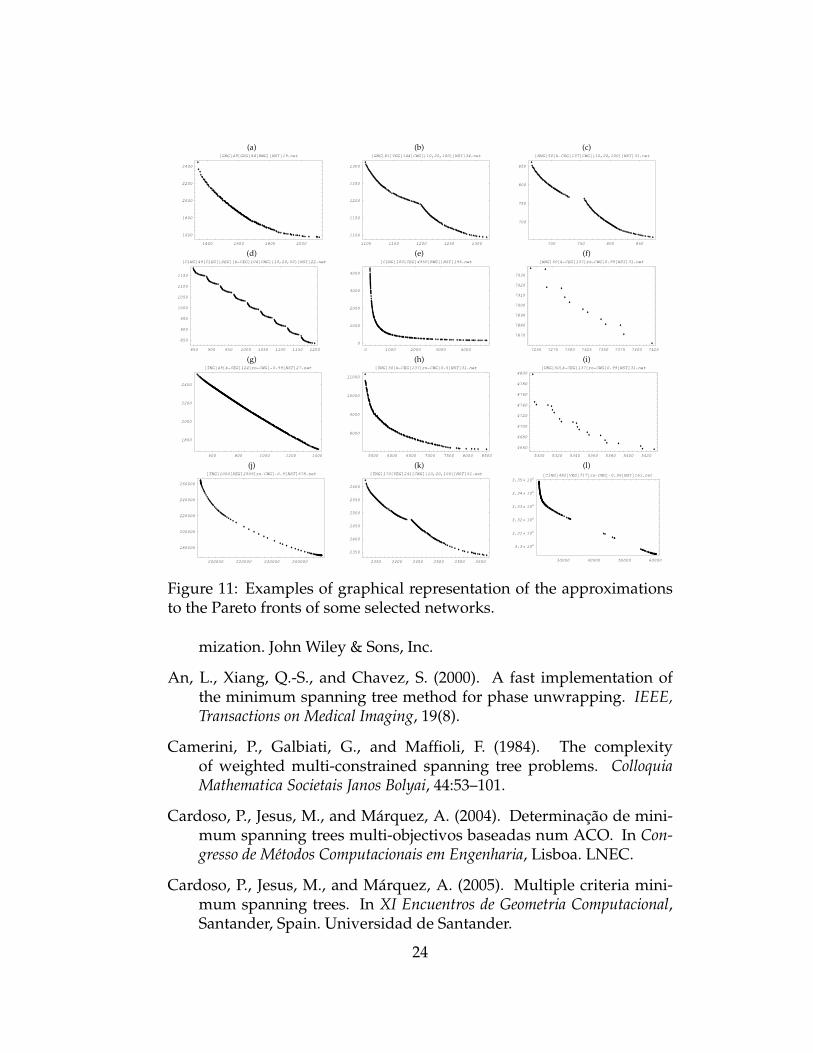
Figures 10 and 11 present the graphical representations of the Paretofronts (obtained with the brute force method) and the approximationssets of some examples. The Pareto approximations are the nondomi-nated set of the union of the solutions returned by the weighted sumand MONACO.

For instance, in Figures 10 (a), (b), (d), (e), (h), and Figures 11 (b), (c),(d) we see sketches of eight concave fronts. In Figures 10 (c), (g), and Fig-ure 11 (g) the solutions of three networks that used the ρ−CWG (with ρequal to −0.99 and −0.9) are depicted. In these cases, the nondominatedset has a relatively large cardinality and the graphical representation isan almost straight line.

7 Conclusions and Future Work

The MOST Project intends to maintain a repository for spanning-tree-related problems. In this installation phase, we considered only the un-constrained minimum spanning trees problem with two objectives. Infuture, and taking into account the pretension of providing real-life prob-lems, this library must contain some other features like, undirected net-works, networks with a larger number of objectives and nodes, differenttopologies, and different instances of the spanning trees problem.

We have established a set of network generators, that are combina-tions of three types: nodes, edges, and weights generators. These net-work generators produce a diversified set of fronts, capable of definingan also diversified number of difficulties in the optimization process. Ac-companying the problem instances, the results obtained using a bruteforce method (whenever the dimension of the problem makes it pos-sible), a weighted sum method or a meta-heuristics are presented. Inparticular, we used the MONACO meta-heuristic.

On our behalf, improvements to the MONACO’s algorithm and other

22

(a)* (b)* (c)

350 400 450 500

350

400

450

500

@ClNGD20@ClEGD@DEGD@CEGD45@CWGD810,20,50<@NSTD9.net

1400 1600 1800 2000 2200 2400

14800

15000

15200

15400

15600

15800

16000

16200

@ClNGD20@ClEGD@DEGD@[email protected]@NSTD7.net

0 2500 5000 7500 10000 12500 15000

0

2000

4000

6000

8000

10000

12000

14000

@ClNGD20@[email protected]@NSTD23.net

(d) (e)* (f)

275 300 325 350 375 400 425

275

300

325

350

375

400

425

@TNGD20@CEGD190@CWGD810,20,100<@NSTD23.net

350 360 370 380 390 400

350

360

370

380

390

400

410

@GNGD25@GEGD40@CWGD810,20,50<@NSTD8.net

0 200 400 600 800 1000

0

200

400

600

800

1000

@GNGD20@CEGD190@[email protected]

(g) (h) (i)

4000 6000 8000 10000 12000

12000

14000

16000

18000

@NNGD20@[email protected]@NSTD10.net

320 340 360 380 400 420 440

320

340

360

380

400

420

440

@NNGD20@DEGD50@CWGD810,20,100<@NSTD11.net

4200 4400 4600 4800 5000

6100

6200

6300

6400

6500

6600

6700

6800

@NNGD20@[email protected]@NSTD10.net

(j) (k) (l)

4000 6000 8000 10000 12000

4000

6000

8000

10000

12000

14000

@UNGD20@[email protected]@NSTD23.net

2840 2860 2880 2900

3060

3062.5

3065

3067.5

3070

3072.5

3075

@UNGD20@[email protected]@NSTD11.net

3000 3200 3400 3600 3800 4000

3500

3750

4000

4250

4500

4750

5000

5250

@UNGD20@[email protected]@NSTD11.net

Figure 10: Examples of graphical representation of the approximationsto Pareto fronts and exact fronts(*), for some selected networks.

meta-heuristical approaches are being studied in order to compute betterPareto approximations as well as to deal with larger networks.

Finally, we reinforce the ideas:

• MOST Project must be a dynamic venture, open to the free utiliza-tion of the enclosed problems;

• MOST is also open to the spanning trees investigators commu-nity contributions (new problems, solutions improvements, site im-provements,...).

References

Aarts, E. and Lenstra, J. (1997). Local Search in Combinatorial Optimiza-tion. Wiley-Interscience Series in Discrete Mathematics and Opti-

23

(a) (b) (c)

1400 1600 1800 2000

1600

1800

2000

2200

2400

@GNGD49@GEGD84@[email protected]

1100 1150 1200 1250 1300

1100

1150

1200

1250

1300

@GNGD81@VEGD144@CWGD810,20,100<@NSTD34.net

700 750 800 850

700

750

800

850

@NNGD50@k-CEGD137@CWGD810,20,100<@NSTD31.net

(d) (e) (f)

850 900 950 1000 1050 1100 1150 1200

850

900

950

1000

1050

1100

1150

@ClNGD49@ClEGD@DEGD@k-CEGD104@CWGD810,20,50<@NSTD22.net

0 1000 2000 3000 4000

0

1000

2000

3000

4000

@ClNGD100@CEGD4950@[email protected]

7250 7275 7300 7325 7350 7375 7400 7425

7870

7880

7890

7900

7910

7920

7930

@NNGD50@[email protected]@NSTD31.net

(g) (h) (i)

600 800 1000 1200 1400

1800

2000

2200

2400

@TNGD49@[email protected]@NSTD27.net

5500 6000 6500 7000 7500 8000 8500

8000

9000

10000

11000

@UNGD50@[email protected]@NSTD31.net

5300 5320 5340 5360 5380 5400 5420

4660

4680

4700

4720

4740

4760

4780

4800

@UNGD50@[email protected]@NSTD31.net

(j) (k) (l)

200000 220000 240000 260000

180000

200000

220000

240000

260000

@TNGD1000@[email protected]@NSTD678.net

2350 2400 2450 2500 2550 2600

2350

2400

2450

2500

2550

2600

@TNGD170@VEGD241@CWGD810,20,100<@NSTD51.net

30000 40000 50000 60000

3.3 ´ 106

3.31 ´ 106

3.32 ´ 106

3.33 ´ 106

3.34 ´ 106

3.35 ´ 106

@ClNGD482@[email protected]@NSTD161.net

Figure 11: Examples of graphical representation of the approximationsto the Pareto fronts of some selected networks.

mization. John Wiley & Sons, Inc.

An, L., Xiang, Q.-S., and Chavez, S. (2000). A fast implementation ofthe minimum spanning tree method for phase unwrapping. IEEE,Transactions on Medical Imaging, 19(8).

Camerini, P., Galbiati, G., and Maffioli, F. (1984). The complexityof weighted multi-constrained spanning tree problems. ColloquiaMathematica Societais Janos Bolyai, 44:53–101.

Cardoso, P., Jesus, M., and Marquez, A. (2004). Determinacao de mini-mum spanning trees multi-objectivos baseadas num ACO. In Con-gresso de Metodos Computacionais em Engenharia, Lisboa. LNEC.

Cardoso, P., Jesus, M., and Marquez, A. (2005). Multiple criteria mini-mum spanning trees. In XI Encuentros de Geometria Computacional,Santander, Spain. Universidad de Santander.

24

Chang, Y., Bergman, L., Castelli, V., Li, C., Lo, M., and Smith, J. (2000).The onion technique: indexing for linear optimization queries. SIG-MOD Rec., 29(2):391–402.

Cirasella, J., Johnson, D., McGeoch, L., and Zhang, W. (2001). The asym-metric traveling salesman problem: Algorithms, instance genera-tors, and tests. Lecture Notes in Computer Science, 2153.

Coello-Coello, C., Hernandez-Lerma, O., and Villalobos-Arias, M.(2005). Foundations of Genetic Algorithms: 8th International Workshop.Lecture Notes in Computer Science. Springer.

de Berg, M., van Kreveld, M., Overmars, M., and Schwarzkopf, O. (1997).Computational Geometry - Algorithms and Applications. Springer-Verlag, Berlin.

Deb, K. (2001). Multi-objective Optimization using Evolutionary Algorithms.John Wiley & sons.

Deb, K., Thiele, L., Laumanns, M., and Zitzler, E. (2002). Scalable multi-objective optimization test problems. In In Congress on EvolutionaryComputation (CEC’2002), volume 1, pages 825–830, Piscataway, NewJersey.

Dorigo, M., Bonabeau, E., and Theraulaz, G. (1999). Swarm Intelligence:From Natural to artificial Systems. Oxford University Press.

Dorigo, M. and Stutzle, T. (2004). Ant Colony Optimization. MIT Press.

Gent, I. and Walsh, T. (1999). Principles and Practice of Constraint Program-ming - CP99, chapter CSPlib: A Benchmark Library for Constraints.Lecture Notes in Computer Science. Springer.

Glover, F. and Laguna, M. (1997). Tabu Search. Kluwer Academic Pub-lishers.

Hajic, J., McDonald, R., Pereira, F., and Ribarov, K. (2005). Non-projectivedependency parsing using spanning tree algorithms. In Human Lan-guage Technology Conference, Vancouver, Canada.

Hamacher, H. and Ruhe, G. (1994). On spanning tree problems withmultiple objective. Annals of operation research, 52:2309–230.

25

Jaszkiewicz, A. (2001). Multiple Objective Metaheuristic Algorithms forCombinatorial Optimization. PhD thesis, Poznan University of Tech-nology.

Johnson, D. and McGeoch, L. (1997). Local Search in Combinatorial Opti-misation, chapter The Traveling Salesman Problem: A Case Study inLocal Optimization, pages 215–310. E. Aarts and J. Lenstra (editors).John Wiley and Sons Ltd.

Jungnickel, D. (1999). Graphs, Networks and Algorithms, volume 5 of Algo-rithms and Computation in Mathematics. Springer-Verlag, Berlin.

Kirkpatrick, S., Gelatt, C., and Vecchi, M. (1983). Optimization by simu-lated annealing. Science, 220, 4598(4598):671–680.

Knowles, J. and Corne, D. (2001). Benchmark problem generators and re-sults for the multiobjective degree-constrained minimum spanningtree problem. In Proceedings of the Genetic and Evolutionary Compu-tation Conference (GECCO-2001), pages 424–431. Morgan KaufmannPublishers, San Francisco, California.

Knowles, J. and Corne, D. (2002). On metrics for comparing non-dominated sets. In Congress on Evolutionary Computation (CEC 2002),volume 1.

Mostaghim, S., Teich, J., and Tyagi, A. (2002). Comparison of data struc-tures for storing Pareto-sets in MOEAs. In Evolutionary Computation(CEC’2002), volume 1, IEEE Service Center, Piscataway, New Jersey.

Pinto, D., Barn, B., and Fabregat, R. (2005). Multi-objective multicastrouting based on Ant Colony Optimization. In CCIA 2005, L’Alguer.

Pirzadeh, H. (1999). Computational geometry with the rotating callipers.Master’s thesis, McGill University, Canada.

Poulos, M., Evangelou, A., Magkos, E., and Papavlasopoulos, S. (2004).Fingerprint verification based on image processing segmentationusing an onion algorithm of computational geometry. In Sixth Int.Conf. on Mathematics Methods in Scattering Theory and Biomedical Tech-nology (BIOTECH’6).

Sack, J.-R. and Urrutia, J. (2000). Handbook of Computational Geometry.Elsevier Science, North-Holland.

26

Shioura, A., Tamura, A., and Uno, T. (1997). An optimal algorithm forscanning all spanning trees of undirected graphs. SIAM Journal onComputing, 26(3).

Toussaint, G. (1983). Solving geometric problems with the rotatingcalipers. In Proceedings of IEEE MELECON’83, Athens, Greece.

Vose, M. (1999). The Simple Genetic Algorithm: Foundations and Theory.MIT Press,.

Zitzler, E., Thiele, L., Laumanns, M., Fonseca, C., and Fonseca, V. (2003).Performance assessment of multiobjective optimizers: An analysisand review. IEEE Transactions on Evolutionary computation, 7(2).

27