MULTIPLE IMPUTATION METHODS FOR STATISTICAL DISCLOSURE CONTROL by Di An A dissertation submitted in partial fulfillment of the requirements for the degree of Doctor of Philosophy (Biostatistics) in the University of Michigan 2008 Doctoral committee: Professor Roderick J.A. Little, Chair Professor Myron P. Gutmann Professor Trivellore E. Raghunathan Assistant Professor Michael R. Elliott

Welcome message from author
This document is posted to help you gain knowledge. Please leave a comment to let me know what you think about it! Share it to your friends and learn new things together.
Transcript

MULTIPLE IMPUTATION METHODS FOR STATISTICAL DISCLOSURE CONTROL
by
Di An
A dissertation submitted in partial fulfillment of the requirements for the degree of
Doctor of Philosophy (Biostatistics)
in the University of Michigan 2008
Doctoral committee: Professor Roderick J.A. Little, Chair Professor Myron P. Gutmann Professor Trivellore E. Raghunathan Assistant Professor Michael R. Elliott

© Di An 2008

ii
To my husband, my parents, aunt Junfu and aunt Yuan
And in loving memory of my grandmother

iii
Acknowledgements
I would like to express my appreciation to those people who helped me with my doctoral
study and my dissertation. First I would like to thank my advisor Dr. Roderick Little for
everything he has taught me. I would never have accomplished this dissertation without
his support and guidance. I thank Dr. Trivellore Raghunathan for his advice and
comments on various aspects in my research, thank Dr. Michael Elliott and Dr. Myron
Gutmann for serving on my dissertation committee and dedicating their time and effort to
my dissertation, and thank Dr. James W. McNally for his contribution to one of our
papers. I also thank the faculty, staff and my fellow students in Biostatistics.
Personally, I would like to thank my husband Feilong Chen, who has always been
devoted and supportive. His love and encouragement helped me through every step of
my doctoral study. I am especially grateful to my father Shuyuan An for sacrificing so
much for my education; without him I would never have the opportunity to complete the
doctoral study. I also thank my mother Ying Yao, who always has faith in me. At last, I
want to thank my aunt Junfu and aunt Yuan, who gave me a lot of support and comfort
when I was having a hard time.

iv
Table of Contents
Dedication………………………………………………………………………………...ii
Acknowledgements……….………………………………………………………....…...iii
List of Tables………………………………………………………………………..........vi
List of Figures…………………………………………………………………………..viii
Chapter I Introduction.........................................................................................................................1
I.1 Statistical disclosure control..................................................................................1 I.2 Multiple imputation methods of SDC ...................................................................2 I.3 Disclosure limitation of extreme values in microdata ...........................................3
Chapter II Multiple Imputation: An Alternative to Top-coding for Statistical Disclosure Control.....6
Abstract .......................................................................................................................6 II.1 Introduction ..........................................................................................................6 II.2 Methods of statistical disclosure control..............................................................9 II.3 Methods of inference for the mean ....................................................................10 II.4 Simulation study.................................................................................................13
II.4.1 Study design ............................................................................................13 II.4.2 Results .....................................................................................................14
II.5 Application .........................................................................................................16 II.5.1 Data analysis ...........................................................................................17 II.5.2 Results .....................................................................................................17
II.6 Study of SDC methods with covariates..............................................................18 II.6.1 Simulation Study.....................................................................................18 II.6.2 Application in Chinese income data........................................................19
II.7. Discussion .........................................................................................................20 Acknowledgments.....................................................................................................25 Appendix II.1: PMI method for log-normal model and power-transformed normal model.........................................................................................................................33 Appendix II.2: EM algorithm for log-normal model ................................................34
Chapter III Extensions of Multiple Imputation Methods as Disclosure Control Procedure for Multivariate Data ..............................................................................................................36
Abstract .....................................................................................................................36 III.1 Introduction.......................................................................................................36

v
III.2 Methods of statistical disclosure control...........................................................38 III.2.1 Previous SDC methods ..........................................................................39 III.2.2 Extensions of MI methods for multivariate data....................................40
III.3 Methods of inference ........................................................................................41 III.4 Simulation study ...............................................................................................43
III.4.1 Study design...........................................................................................43 III.4.2 Results....................................................................................................45 III.4.3 Results from regression of X1 on X2 and imputed X3 ...........................49
III.5 Application........................................................................................................50 III.5.1 Data analysis ..........................................................................................51 III.5.2 Results....................................................................................................51
III.6 Discussion .........................................................................................................52 Acknowledgments.....................................................................................................55 Appendix III.1: Regression-based parametric MI methods for log-normal model and power-transformed normal model.............................................................................71
Chapter IV A Multiple Imputation Approach to Disclosure Limitation for High-age Individuals in Longitudinal Studies .........................................................................................................73
Abstract .....................................................................................................................73 IV.1 Introduction.......................................................................................................74 IV.2 Methods ............................................................................................................77
IV.2.1 SDC methods for longitudinal data .......................................................77 IV.2.2 Methods of inference .............................................................................79
IV.3 Simulation study ...............................................................................................80 IV.3.1 Study design...........................................................................................80 IV.3.2 Results....................................................................................................81
IV.4 Application in Charleston Heart Study data .....................................................83 IV.4.1 Primary data analysis.............................................................................83 IV.4.2 Results from SDC methods ...................................................................84
IV.5 Discussion.........................................................................................................85 Acknowledgments.....................................................................................................87
Chapter V Conclusion and Discussion ...............................................................................................93
Bibliography……………………………………………………………………………..98
List of Tables
Table
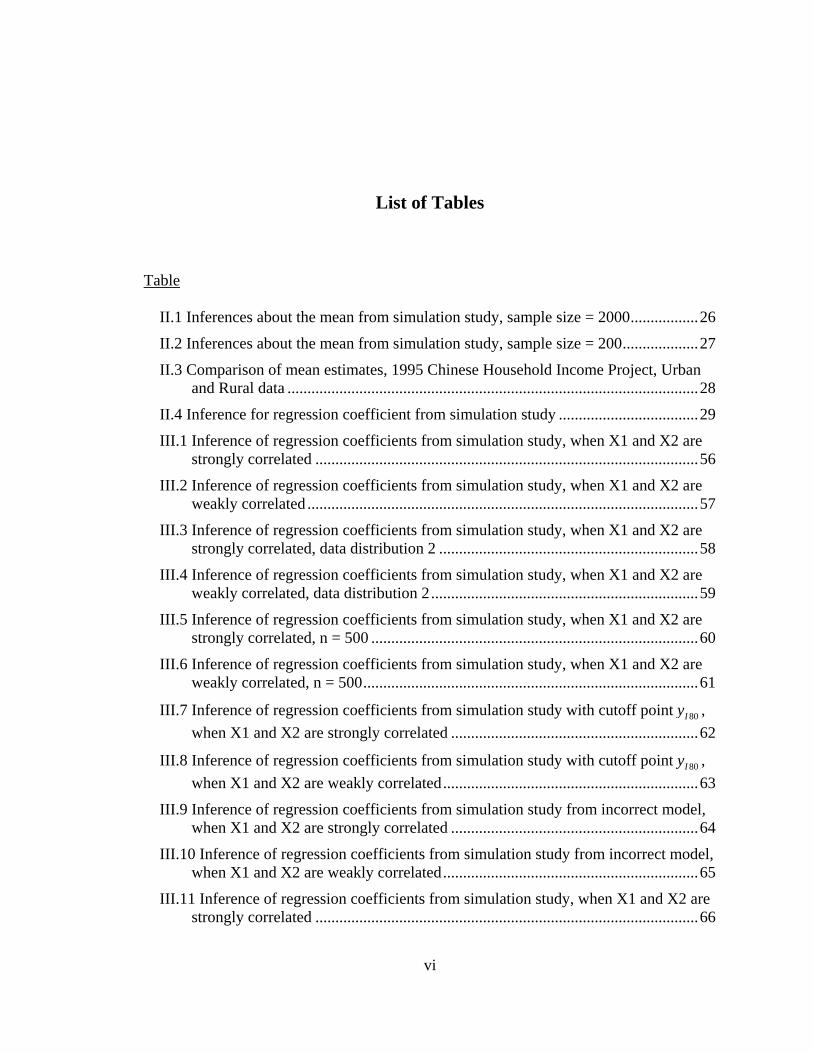
II.1 Inferences about the mean from simulation study, sample size = 2000.................26
II.2 Inferences about the mean from simulation study, sample size = 200...................27
II.3 Comparison of mean estimates, 1995 Chinese Household Income Project, Urban and Rural data .......................................................................................................28
II.4 Inference for regression coefficient from simulation study ...................................29
III.1 Inference of regression coefficients from simulation study, when X1 and X2 are strongly correlated ................................................................................................56
III.2 Inference of regression coefficients from simulation study, when X1 and X2 are weakly correlated ..................................................................................................57
III.3 Inference of regression coefficients from simulation study, when X1 and X2 are strongly correlated, data distribution 2 .................................................................58
III.4 Inference of regression coefficients from simulation study, when X1 and X2 are weakly correlated, data distribution 2...................................................................59
III.5 Inference of regression coefficients from simulation study, when X1 and X2 are strongly correlated, n = 500 ..................................................................................60
III.6 Inference of regression coefficients from simulation study, when X1 and X2 are weakly correlated, n = 500....................................................................................61
III.7 Inference of regression coefficients from simulation study with cutoff point 80Iy , when X1 and X2 are strongly correlated ..............................................................62
III.8 Inference of regression coefficients from simulation study with cutoff point 80Iy , when X1 and X2 are weakly correlated................................................................63
III.9 Inference of regression coefficients from simulation study from incorrect model, when X1 and X2 are strongly correlated ..............................................................64
III.10 Inference of regression coefficients from simulation study from incorrect model, when X1 and X2 are weakly correlated................................................................65
III.11 Inference of regression coefficients from simulation study, when X1 and X2 are strongly correlated ................................................................................................66
vi

vii
III.12 Inference of regression coefficients from simulation study, when X1 and X2 are weakly correlated ..................................................................................................67
IV.1 Hazard rate for simulation study, scenario I and II ..............................................88
IV.2 Hazard rate for simulation study, scenario III ......................................................88
IV.3 Simulation study scenario I: inferences of regression coefficients from PH model...............................................................................................................................89
IV.4 Simulation study scenario II: inferences of regression coefficients from PH model...............................................................................................................................89
IV.5 Simulation study scenario III: inferences of regression coefficients from PH model.....................................................................................................................90
IV.6 Estimates of regression coefficients from PH model, original CHS data.............91
IV.7 Estimates of regression coefficients from PH model, CHS data after SDC.........92

viii
List of Figures
Figure
II.1 Tails of the Data Distributions in Simulation Study ..............................................30
II.2 Deleted and imputed values for square-root-normal data (n=2000) ......................30
II.3 Deleted and imputed values for 1995 Chinese household income project, urban data........................................................................................................................31
II.4 Deleted and imputed values for 1995 Chinese household income project, rural data...............................................................................................................................31
II.5 Standardized regression coefficients, after versus before imputation....................32
III.1 Standardized regression coefficients, after versus before unconditional imputation...............................................................................................................................68
III.2 Standardized regression coefficients, after versus before stratified imputation. ..69
III.3 Standardized regression coefficients, after versus before regression-based imputation. ............................................................................................................70

Chapter I
Introduction
I.1 Statistical disclosure control
The explosion of collection on private data raises concerns about guarding the privacy of
survey respondents now more than ever. Statistical disclosure control (SDC) is a class of
procedures that deliberately alter data collected by statistical agencies before release to
the public, to prevent the identity of survey respondents from being revealed. These
methods have increased in importance, with the extensive use of computers and the
internet. Inevitably, statistical agencies are confronted with the trade-off between data
protection and data utility. The goal of SDC methods is to find a balance for this
dilemma, by reducing the risk of disclosure to acceptable levels, while releasing a dataset
that provides as much useful information as possible for researchers. One aspect of this is
the ability to draw valid statistical inferences from the altered data.
Various SDC techniques have been established to preserve confidentially,
including global recoding and local suppression, swapping data values for randomly
selected units (Dalenius and Reiss, 1982), or adding random noise (Fuller 1993). These
methods involve perturbing and masking of the original data. Though the model-free
nature makes them easy to apply, these methods somewhat distort the statistical structure
of the data and make analysis difficult for data user.
1

I.2 Multiple imputation methods of SDC
Rubin (1993) proposes to release fully synthetic data based on multiple imputation (MI)
methods. In his proposal, an imputation model is built from the original survey data and
data values in the population are imputed by draws from the predictive distribution based
on the model. The imputation process is repeated several times and a random sample
drawn from each imputed dataset is released to the public. A major attraction of this
method is that full protection of confidentiality is achieved, since no actual values from
the original data are released. Besides, under well-specified imputation model, valid
inference for variant estimands can be obtained with simple combining rules
(Raghunathan 2003, Reiter 2002, 2005a). Fully synthetic data also have benefit for data
utility, as geographic information for small area can be released, which enables data user
to perform analysis in small area. However, model specification is challenging for this
method, as it requires building a statistical model for the whole population. Moreover,
since the synthetic data need to preserve the same relationship as the original data, the
accuracy of the statistical model is crucial to valid inferences from synthetic data, and a
mis-specified model leads to distorted results from data users’ analyses.
Little (1993) suggests limiting imputation to a set of key variables that contain
identification information and releasing partially synthetic data as a mixture of actual and
multiply-imputed data values. This method retains the advantage of synthetic data but is
more practical than simulating the entire data set, since model mis-specification is less of
an issue for simulating certain variables than simulating the entire population. Some other
approaches to partial synthesis method are described in Kennickell (1997), Little, Liu and
Raghunathan, (2004), and Abowd and Woodcock (2004). Reiter (2003) specifies MI
2

combining rule for partially synthetic data, with estimate of variance calculated
differently from the original formula for missing data in Little and Rubin (2002). Inspired
by this approach, this dissertation targets the imputation of a small number (one or two)
of variables subject to disclosure limitation.
I.3 Disclosure limitation of extreme values in microdata
A number of confidentiality concerns are raised by extreme values of a variable. For
example, in surveys that include income, extremely high income values are considered to
have the potential to reveal the identity of respondents. These values are generally
referred to as sensitive values and require modification before release to the public. The
Health Insurance Portability and Accountability Act (HIPAA) privacy rule also restricts
release of all age values over 89 in health survey data. Top-coding is a simple and
common SDC method for handling this situation. It prevents disclosure on the basis of
extreme values of a variable, by censoring values above a pre-chosen “top-code”. For
example, in the Survey of Income and Program Participation, the U.S. Census Bureau
top-codes monthly income at $8,333 in the 1990-1993 panels, such that all values $8,333
or more are now represented by $8,333.
Data analyst can apply several approaches to analyze top-coded data, such as
categorizing the top-coded variable to pool top-coded cases into one category, or treating
the top-coded values as the true values. In addition, the data user can treat the extreme
values as censored; and calculate estimates (e.g., maximum likelihood estimate) under the
assumed statistical model, or apply an imputation method to the top-coded dataset and fill
in the censored values. These procedures all have limitations for data user: they more or
3

less distort data distributions, require complicated custom algorithms, or are sensitive to
model assumption about the right tail of the distribution.
Another limitation of top-coding lies in the treatment of high-age individuals in
longitudinal datasets, where disclosure limitation is particularly challenging, since
information about an individual accumulates with repeated measures over time. Because
of the risk of disclosure, ages of very old respondents can often not be released; in
particular this is a specific stipulation of HIPAA privacy rule for the release of health
data for individuals. Top-coding of individuals beyond a certain age (say 80) is a standard
way of dealing with this issue, and it may be adequate for cross-sectional data, since the
number of cases affected may be modest. However, this approach seriously limits the
ability to do longitudinal analysis, particularly survival analyses with chronological age
being a key variable of interest.
This problem arises in the Charleston Heart Study (Nietert et al., 2000), a
longitudinal study that collects data over 40 years (1960-2000). For longitudinal data
from this study to be included in the data archive at the University of Michigan,
individual ages beyond age 80 cannot be disclosed, given the geographic specificity of
the respondents. Also, given the longitudinal nature of the data, a top-coding approach
would need to be applied to all individuals aged 40 or older in 1960, which makes
survival analyses almost impossible.
In this dissertation, I develop MI alternatives to top-coding that allow better
inferences for the data user using simple MI combining rules, while preserving the SDC
benefits of top-coding. Adjusting the partially synthetic approach to our specific problem,
we delete the data values greater than a cutoff point, which is chosen to be smaller than
4

the top-code to achieve a mixing of sensitive and non-sensitive values, and apply MI to
fill in these values. We then release multiple imputed datasets to the public. Data users
can apply MI combining rules (Reiter 2003) to obtain valid inferences.
I propose non-parametric and parametric MI methods. The non-parametric
method is a hot-deck procedure, where we replace the deleted values with values
randomly drawn with replacement from the set of deleted values. The parametric method
is Bayesian, and assumes a model for the data, draws model parameters from their
posterior distribution and then imputes the deleted values with random draws from the
posterior predictive distribution.
This dissertation is organized as follows. Chapter II presents our SDC approaches
and describes corresponding methods of inference for a population mean. We compare
estimates calculated from our imputed datasets with estimates from the original and top-
coded dataset in simulation study and application in the 1995 Chinese household income
project. Chapter III provides extension of the MI methods in Chapter II in regression
analysis, where the outcome is subject to top-coding and assesses inferences of estimates
of regression coefficients. Chapter IV describes SDC approaches for longitudinal data
and applies these methods in survival analysis of simulated data and data from the
Charleston Heart Study. Chapter V presents conclusions and discusses future work.
5

Chapter II Multiple Imputation: An Alternative to Top-coding for Statistical
Disclosure Control
Abstract
Top-coding of extreme values of variables like income is a common method of statistical
disclosure control, but it creates problems for the data analyst. This article proposes two
alternative methods to top-coding for SDC based on multiple imputation (MI). We show
in simulation studies that the MI methods provide better inferences of the publicly-
released data than top-coding, using straightforward MI methods of analysis, while
maintaining good SDC properties. We illustrate the methods on data from the 1995
Chinese household income project.
Keywords: confidentiality, disclosure protection, multiple imputation
II.1 Introduction
Statistical disclosure control (SDC) is a class of procedures that deliberately alter data
collected by statistical agencies before release to the public, to prevent the identity of
survey respondents from being revealed. These methods have increased in importance,
with the extensive use of computers and the internet. The goal of SDC methods is to
reduce the risk of disclosure to acceptable levels, while releasing a dataset that provides
as much useful information as possible for researchers. One aspect of this is the ability to
draw valid statistical inferences from the altered data.
6

Top-coding is a simple and common SDC method that seeks to prevent disclosure
on the basis of extreme values of a variable, by censoring values above a pre-chosen
“top-code”. For example, in surveys that include income, extremely high income values
are considered to be sensitive and have the potential to reveal the identity of respondents.
By recoding income values greater than a selected “top-code” value to that value,
respondents with very high income have reduced risk of disclosure.
It is left to the analyst to decide how top-coded data are analyzed. One approach is
to categorize the variable so that top-coded cases all fall in one category – this is sensible,
but precludes analyses that treat the variable as continuous. Another approach is to ignore
the fact of top-coding and treat the top-coded values as the truth. This method is
straightforward, but clearly the data distribution is distorted and biased estimates will be
obtained. A better method is to treat the extreme values as censored. Under an assumed
statistical model, maximum likelihood (ML) estimates can be obtained using algorithms
such as the Expectation-Maximization (EM) algorithm (Dempster, Laird and Rubin,
1977). This method is model-based, and should yield good inferences if the model is
correctly specified. But we expect this method to be quite sensitive to model
misspecification, especially when the upper tail of the assumed distribution differs
markedly from that of the true distribution. The data users can also apply an imputation
method to the top-coded dataset and fill in the censored values. A limitation is that the
imputed data fail to reflect imputation uncertainty, and imputations are sensitive to
assumptions about the right tail of the distribution. We propose alternatives to top-coding
that allow better inferences for the data user using simple multiple imputation (MI)
combining rules, while preserving the SDC benefits of top-coding.
7

Multiple imputation has been proposed as a method of SDC (Little, 1993; Rubin,
1993; Little, Liu and Raghunathan, 2004; Reiter, 2003, 2005a, 2005b). An imputation
model is built from the original data and observed values are replaced by draws from the
predictive distribution based on the model. The imputation process is repeated several
times and the imputed datasets are then released to the public. Applying this approach to
our problem, we delete the data values greater than a cutoff point, which is chosen to be
smaller than the top-code to achieve a mixing of sensitive and non-sensitive values, and
apply MI to fill in these values. We then release multiple imputed datasets to the public.
Data users can apply MI combining rules (Reiter 2003) to obtain valid inferences, as
described in Section II.3.
We propose non-parametric and parametric MI methods. The non-parametric
method is a hot-deck procedure, where we replace the deleted values with values
randomly drawn with replacement from the set of deleted values. The parametric method
is Bayesian, and assumes a model for the data, draws model parameters from their
posterior distribution and then imputes the deleted values with random draws from the
posterior predictive distribution.
We compare estimates of the mean of the data from our methods with two
estimates from top-coded data. The first, as described previously, is to treat the top-coded
values as the true values. The second is to treat those values greater than top-code as
censored and apply ML estimation under an assumed model.
We also investigate situations where covariates are present. We use the proposed
MI methods to fill in for deleted values without conditioning on covariates. We then
perform regression analysis on the imputed dataset and compare regression coefficients
8

with those from original and top-coded data. Extensions of our methods that condition on
covariate data are also outlined.
The rest of this paper is organized as follows. Section II.2 presents SDC
approaches, and Section II.3 describes corresponding methods of inference for a
population mean. Section II.4 describes a simulation study to evaluate the approaches in
Section 3, and Section II.5 applies the methods to data from the 1995 Chinese household
income project. Section II.6 considers estimates of regression coefficients for a regression
where the outcome is subject to our disclosure control methods. Section II.7 gives
conclusions and discusses future work.
II.2 Methods of statistical disclosure control
Let Y denote a survey variable (e.g. income) and suppose that values of Y greater than a
particular value are considered too sensitive for release to the public. We consider
the following approaches to SDC.
Ty
(a) Top-coding. Treat as a top-code value, that is, replace values of Y greater than
by . The resulting sample is referred to as “top-coded”.
Ty
Ty Ty
(b) Hot-deck MI (HDMI). Choose a value smaller than . Delete the values of
greater than and replace them with random draws from the set of deleted values. We
choose to achieve a mixing of sensitive and non-sensitive values. We refer to
as the cutoff point.
Iy Ty Y
Iy
TI yy < Iy
(c) Parametric MI (PMI). The HDMI method provides disclosure protection by
scrambling sensitive and non-sensitive values, but it is arguably limited from the point of
view of SDC, since actual sensitive data values are released. The PMI methods address
this concern by releasing data simulated from a parametric model. First, values greater
9

than are deleted, as with HDMI. The model – we consider log-normal model and
power-transformed normal model (the power normal model for short) – is fitted to the
data. Parameters are drawn from their posterior distribution under the assumed model,
and deleted values are imputed with draws from their predictive distribution. See
Appendix II.1 for details.
Iy
Write the complete data as ret del( , )Y Y Y= , where denotes the retained values
and denotes the deleted values beyond the cut-off. We consider two versions of PMI,
labeled PMIC and PMID. For PMIC, we draw the parameter
retY
delY
φ of the model for the data
Y from its posterior distribution given the complete data Y, that is:
PMIC: . * ~ ( | )P Yφ φ
We then draw deleted values from the truncated predictive distribution
* *del ~ ( | , )IY P Y Y y φ> .
For PMID, we apply the parametric model to the deleted data , and draw delY φ from its
posterior distribution given : delY
PMID: *del~ ( | )P Yφ φ
The next step is similar to PMIC method, except that we draw deleted values from the
non-truncated predictive distribution. PMID is less efficient than PMIC since it models
the deleted data and fails to exploit fully the information in Y when drawing values of
parameters. However, modeling the deleted data only as in PMID provides useful
robustness to model misspecification, as we shall see below.
II.3 Methods of inference for the mean
We first consider the properties of these SDC methods for inferences about the mean of a
variable Y subject to top-coding. Some comments concerning inference for other
10

parameters are provided in Sections II.6 and II.7. The following estimates and associated
standard errors are considered:
(1) Before Deletion (BD): The sample mean of original data 1 2( , ,..., )ny y y prior to SDC
is
∑=
=n
iiy
n 11
1θ̂ . (1)
This estimate is used as a benchmark for comparing SDC methods.
(2) Top-coding (TC): The sample mean of top-coded dataset, namely
21
1ˆn
iti
yn
θ=
= ∑ , (2)
where it iy y= when i Ty y< and it Ty y= when i Ty y≥ . This approach is obviously
biased, and our objective is to improve on it with other methods.
(3) Log-normal ML (LNML): The ML estimate based on the log-normal model,
computed by the EM algorithm (Appendix II.2). The log-normal is chosen as a
convenient model for right-skewed data, but we emphasize that other models could be
considered.
The standard errors for methods (1) – (3) are computed by the bootstrap, with B =
100 bootstrap samples.
The five remaining methods are all based on MI, and create D sets of imputations
for values beyond the chosen cut-point Iy ; D imputed datasets are thus created, where
for the d th imputed dataset , where ( ) ( ) ( ) ( )1 2( , ,..., )d d d d
nY y y y= ( )di iy y= if i Iy y< and
is the d th MI draw if
( )diy
i Iy y≥ . The MI estimate is then
∑=
=D
d
dMI D 1
)(ˆ1ˆ θθ , (3)
11

where ( )ˆ dθ is the sample mean of d th dataset. The MI estimate of variance is
ˆ( ) /MI MIT Var W Bθ= = + D , (4)
where ( )1
/D dd
W W=
=∑ D is the average of the within-imputation variances for
imputed dataset d, and is the between-imputation
variance. The formula (4) differs from the original MI formula for missing data (where B
is multiplied by a factor (D+1)/D, see e.g. Little and Rubin, 2002, p86), for reasons
discussed in Reiter (2003). Imputations for these MI methods are created as follows:
( )dW
)1/()ˆˆ(1
2)( −−= ∑ =DB D
d MId θθ
(4) Hot-deck MI (HDMI): Imputations are drawn randomly with replacement from the set
of values beyond the cut-off Iy .
(5) Log-normal MIC (LNMIC): Imputations are posterior predictions from a log-normal
model fitted to the complete data before deletion.
(6) Log-normal MID (LNMID): Imputations are posterior predictions from a log-normal
model fitted to the deleted data beyond the cut-off.
(7) Power-normal MIC (PNMIC): Imputations are posterior predictions from the power-
normal model, the power-transformed normal distribution fitted to the full data before
deletion. For convenience the power transformation is estimated by ML, and parameters
are drawn from the full-data posterior distribution treating the power transformation as
known. An alternative approach is to draw the power from its posterior distribution as
well, but we made use of the widely available ML routine box.cox.powers( ) in R (R
project, 2007) in our calculations.
(8) Power-normal MID (PNMID): Imputations are posterior predictions from the power-
normal model, fitted to the deleted data beyond the cut-off.
12

II.4 Simulation study
A simulation study was carried out to evaluate and compare the SDC methods in Section
II.3. We computed point estimates of means and the corresponding variances and
confidence intervals from the imputed datasets, and compared them with those calculated
from the original dataset prior to SDC.
II.4.1 Study design
Datasets were generated from the following four distributions, all with mean 1:
Exponential (1), gamma (1.25, 0.8), lognormal (-0.2, 0.4) and square-root normal (0.9,
0.19) (variances of these distributions are 1, 0.8, 0.49 and 0.69, respectively). Figure II.1
shows the form of these distributions beyond their approximate upper 10th percentile. For
each simulated dataset, we calculated the eight mean estimates and their corresponding
variances as discussed in Section II.3. To assess the validity of inferences, we calculated
the 95% confidence intervals (CI’s) based on the usual normal approximation, and
computed the proportion of CI’s that contain the true mean. For parametric estimates in
Section II.3, the simulated data distributions are allowed to differ from those assumed in
the statistical models, in order to provide an assessment of sensitivity to model
misspecification.
In our simulations we chose the 95th percentile of the population distribution as
the top-code value . Denote by the number of sensitive sample values greater
than . We studied two alternative values for the cutoff point :
Ty Sn
Ty Iy 90Iy , the value with
larger values in the sample, and 2 Sn 80Iy , the value with larger values in the sample.
These values correspond approximately to the 90th and 80th percentile values of the
4 Sn
13

distribution, and for this reason we label the version of a method * that uses cutoff 90Iy
“*90” and the version that uses cutoff 80Iy “*80”.
Clearly the disclosure risk is reduced by increasing the fraction of non-sensitive
values that are imputed. A simple measure of the risk of disclosure is the proportion of
multiple-imputed values beyond the top-code value Ty . For all the MI methods, this is
approximately 50% when the cutoff point is 90Iy , and approximately 25% when the
cutoff point is 80Iy .
II.4.2 Results
Tables II.1 and II.2 present simulation results for sample sizes 2000 and 200,
respectively. Results are based on 500 data sets for each model. We set B = 100 for the
number of bootstrap samples. For both NPMI and PMI methods, we created D = 5
imputed datasets. As expected, TC underestimates the mean and has poor confidence
coverage, particularly for the n = 2000 sample size where bias is a relatively large
component of the RMSE. The HDMI methods (HDMI90 and HDMI80) have minimal
bias and close to nominal coverage for all the simulated populations, with small increases
in RMSE and CI width compared with the BD estimate. LNML dominates other methods
for lognormal data, but has serious bias and very poor confidence coverage for the other
data sets, suggesting marked sensitivity to model specification. The LNMIC methods
have similar properties, although they are less biased and have somewhat better
confidence coverage than LNML when the model is mis-specified. The LNMID methods
are much more robust than their LNMIC counterparts, yielding minimal bias and good
confidence coverage for all problems simulated.
14

The PNMIC methods do consistently well in terms of RMSE. Confidence
coverage is close to the nominal value, except for exponential data with n = 2000 where
coverage is a little low. This suggests that the power normal model yields good fits to the
range of models simulated. The PNMID methods also perform well in terms of bias and
confidence coverage, but they are less efficient than the PNMIC methods.
When lowering the cutoff point from 90Iy to 80Iy , we observe minor increases in
RMSE for HDMI, LNMID and PNMIC, and LNMIC when correctly specified. More
substantial increases in RMSE are seen for PNMID, and LNMIC when mis-specified.
The losses in efficiency for HDMI80, LNMID80 and PNMIC80 may be acceptable given
the increase in disclosure protection.
To provide a visual illustration of the imputation methods under potentially mis-
specified models, Figure II.2 shows the original deleted data values and the imputed
values from the HDMI and four PMI methods, with cutoff 90Iy , for one of the simulated
square-root normal data sets with n =2000. Note that the mean of the deleted values is
2.78. The HDMI predictions look similar to the deleted values and have a similar mean,
2.80.
The LNMIC predictions are too severely skewed and have some extreme
predictions, reflecting the damaging effect on predictions in the tail of applying a mis-
specified model to the full data set. The LNMIC predictions average 5.68, a marked
overestimate. In contrast, when the lognormal model is correctly specified, the
predictions track the deleted values well (data not shown). The LNMID predictions have
the shape of a normal distribution, reflecting effects of model misspecification, but their
mean, 2.72, matches the mean of the deleted values well.
15

The PNMIC predictions match the deleted values quite well and have a similar
mean (2.87), reflecting that this model is correctly specified, since the power normal
model includes the square-root normal as a particular case. The PNMID predictions are
more skewed than the deleted values, a reflection that the power normal model does not
fit that well when applied to the deleted values; however these predictions average 2.79,
very close to the mean of the deleted values.
In summary, we see that for inference about the mean, the HDMI method
performs best overall, but has the limitations in terms of SDC noted above. Among the
parametric imputations, LNMID has the best performance and it works almost as well as
HDMI. In particular it gives good estimates of the mean even when the log-normal model
is mis-specified and LNMIC is biased, reflecting the fact that the impact of mis-
specification on the mean is limited when the model is fit to the deleted data. (On the
other hand this method will work less well for large percentiles under mis-specification,
since the imputed distribution in the upper tail is distorted). PNMIC also does quite well,
reflecting that the power-normal model fits the simulated distributions well. The PNMID
method is satisfactory in terms of bias and confidence coverage, but it is considerably
less efficient than PNMIC or LNMIC since it is fitting the larger power-normal model to
the small set of deleted values. The risk of disclosure is reduced when we increase the set
of value being mixed with the sensitive cases, at the expense of some loss of efficiency of
the estimate.
II.5 Application
We applied the above SDC methods to a subset of data from the 1995 Chinese Household
Income Project (Riskin et al.2000). This project was designed to measure the personal
16

income distribution in the People’s Republic of China in 1995. Income information on
both household and individual were recorded for rural and urban areas. Since SDC was
not applied to the released data set, the effectiveness of the various SDC methods can be
readily assessed.
II.5.1 Data analysis
We illustrated application of the SDC methods to both urban and rural individual income
values. After deletion of missing and zero income values, the urban dataset included
15,983 individuals and the rural dataset had 6,296 individuals. We applied the top-
coding, HDMI and PMI methods to the data and compute estimates (1) – (8) described in
Section II.3. The power transformation parameter estimated by the R function was 0.13
for the rural data and 0.45 for the urban data.
II.5.2 Results
Table II.3 displays the results from the data analysis. We plot the original deleted data
values and the imputed values from PMI and HDMI methods using cutoff point 90Iy in
Figure II.3 and II.4 for urban and rural data, respectively.
Predictably, in both urban and rural cases, TC underestimates the mean and yields
an underestimate of standard error because of the reduction in standard deviation from
top-coding. HDMI90 provides the estimate of the mean closest to the BD mean, with a
16% increase in standard error. LNML has a large positive bias, indicating sensitivity to
the lack of fit of the log-normal model for these data. LNMIC90 is also quite biased,
although it performs better than LNML. LNMID90 has negligible bias and a slightly
smaller standard error than BD in both urban and rural data. The power-normal model
estimates PNMIC90 and PNMID90 also have small bias. For urban data, PNMIC90 has
17

relative CI widths less than that from BD, which seems anti-conservative; for the rural
data it has standard error very similar to BD. PNMID90 shows a slight increase in CI
width for urban data but a large increase in CI width for rural data, reflecting difficulties
in fitting this complex model to the deleted data. Changing the cutoff point to 80Iy results
in some increases in bias and standard error for LNMIC80 estimates. Estimates from
HDMI80, LNMID80 and PNMIC80 are still acceptable, as are PNMID80 estimates in the
urban sample. For the rural data, PNMID80 yields an estimate with strikingly large bias
and standard error, the result of some very extreme outliers from imputation. It is
important to check that the method is not creating extreme outliers as in this illustration.
II.6 Study of SDC methods with covariates
To make the situation more complicated and realistic, we now introduce covariates into
our analysis. We use the previous MI methods to impute deleted values, apply a linear
regression model to the imputed data set, calculate estimates of regression coefficients
and compare them with those from the original data. Since the MI methods do not
condition on the covariates, we expect some bias from this procedure; our interest is in
the size of the bias and resulting distortions in confidence coverage.
II.6.1 Simulation Study
Datasets were generated from the following two distributions:
High correlation distribution: ~ Bivariate Normal ⎟⎟⎠
⎞⎜⎜⎝
⎛)log(Y
X⎟⎟⎠
⎞⎜⎜⎝
⎛⎟⎟⎠
⎞⎜⎜⎝
⎛⎟⎟⎠
⎞⎜⎜⎝
⎛38.05593
,6.8
38
Low correlation distribution: ~ Bivariate Normal ⎟⎟⎠
⎞⎜⎜⎝
⎛)log(Y
X⎟⎟⎠
⎞⎜⎜⎝
⎛⎟⎟⎠
⎞⎜⎜⎝
⎛⎟⎟⎠
⎞⎜⎜⎝
⎛38.05.25.293
,6.8
38
Here X is considered as independent variable and Y is dependent variable. For each
simulated dataset, we applied the SDC methods to impute for deleted values and
18

performed linear regression of log(Y) on X. We then calculated the estimates of
regression coefficient, their corresponding variances and confidence coverage, as we did
for the estimates of the mean in Section II.4.
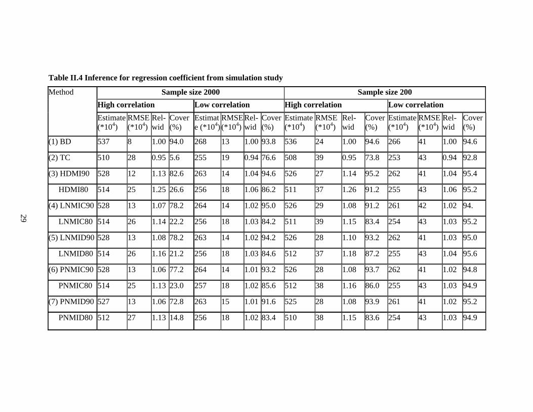
Table II.4 displays results for sample sizes 2000 and 200. For data from the high
correlation distribution, TC underestimates the regression coefficient, with large RMSE
and very poor confidence coverage. HDMI90 also underestimates the coefficient, as is to
be expected since the relationship between the outcome and covariate is attenuated by
randomly “shuffling” the values beyond top-code. Nevertheless it is less biased and has
better coverage than TC. The other PMI90 methods yield almost the same result as
HDMI90. When changing the cutoff point to 80Iy , all MI methods yield estimates with
more bias and RMSE, reduced efficiency and worse confidence coverage. When the data
are from the low correlation distribution, all methods have similar properties, but the MI
methods have satisfactory properties. This suggests that for more moderately correlated
data, the attenuating effect from imputing without conditioning on X is relatively minor.
For the smaller sample size of 200, all methods are improved in terms of confidence
coverage.
II.6.2 Application in Chinese income data
We also consider the impact of the SDC methods on a multiple regression, estimated on a
subset of the urban data in the 1995 Chinese Household Income Project. Our sample
included 10,752 individuals and 10 variables, with the logarithm of income treated as the
dependent variable. The covariates were age, gender, marital status, education level,
occupation, work environment, work intensity, years of work experience and logarithm of
hours worked per week. To simplify the analysis, we only investigate the scenario where
19

the covariates are complete. We applied the top-coding, HDMI and PMI methods to the
data, where the PMI methods were applied to the marginal distribution of the dependent
variable. We again computed estimates of regression coefficients.
We plot standardized regression coefficients after imputation against those from
the original dataset in Figure II.5. We choose HDMI, LNMID and PNMIC as
representations of the MI methods and use the 90th, 80th, 60th and 40th percentiles of the
outcome variable as cutoff points, to assess the effect of increasingly severe imputation.
We observe that with 90Iy , the regression coefficients from the imputed dataset are very
close to those from the dataset before imputation; and imputation with 80Iy also has a
minor effect on the coefficients. This particular case is similar to the low correlation
scenario from simulation study. We conclude that in a situation where the outcome and
covariates are not strongly associated, the proposed MI methods are robust to the failure
of the imputation model to condition on covariates. Lowering cutoff points results in
larger deviation from original coefficients, leading to greater attenuation of the
relationship between outcome and covariates.
II.7. Discussion
Why should the secondary data analyst prefer our proposed MI methods for SDC to top-
coding? First, appropriate treatment of the top-coded data, using methods like maximum
likelihood for censored data, requires custom algorithms that are not widely available in
standard statistical software; as a result we believe that analysts often treat the top-codes
as true values and assume the bias introduced by this will be small. In contrast, MI
inferences only require complete-data methods and simple MI combining rules. Second,
the MI methods tend to be less sensitive than top-coding to model misspecification, as
20

seen in our simulation studies. There are two reasons for this – the random draws from
the predictive distribution provide variability even if the model is wrong, and the MI’s
are based on parameter estimates that use information in the original data that is not
available in the top-coded data. The data producer is also in a better position to assess and
limit model misspecification, since (s)he can compare analyses based on the MI data with
analyses based on the original data. In particular, the imputations from the model can be
compared with the true values.
For the data producer, MI has the advantage that the balance between disclosure
protection and information loss can be controlled by the choice of cut-off and number of
MI’s released. The use of MI allows imputation uncertainty to be propagated, and the
multiple imputations of a particular value enhance disclosure protection by making clear
to a potential snooper that these values are not real.
For inference about the mean, the HDMI, PNMIC and LNMID methods were
decisively superior to top-coding in our simulations. It is clear that treating the top-coded
data as the observed data yields bias, the size of which depends on the fraction of cases
top-coded and the extremity of the top-code. The ML methods based on top-coded data
are harder to implement for the data user, and are vulnerable to model misspecification.
Of our preferred MI methods, the HDMI method produces excellent inferences, but has
limitations as an SDC method, since original values in the data set are retained. The
PNMIC and LNMID methods both yield good inferences for the mean, with the PNMIC
yielding imputations that match well the distribution of the deleted values. The LNMIC
method is vulnerable to misspecification, and the PNMID yields good conference
coverage but tends to be less efficient than LNMID and PNMIC.
21

We chose the log-normal and power normal models to illustrate parametric MI,
since they are commonly used to model skewed data; they are not universal, and the MI
approach could be applied by the data producer with other models that are more suitable
for the data at hand. MI based on a model fit to all the data (as in the “C” methods) is
efficient, but vulnerable to model misspecification. Hence if this approach is adopted,
attention to good model specification is needed – in particular, it is important to check
that the distribution of the imputed values in the tail is similar to the distribution of the
deleted values.
MI based on a model fitted to the deleted values alone (the “D” methods) involves
some loss of efficiency, but is more robust to model misspecification, since the model is
being fitted to the data that are being deleted. Here simpler models worked well for the
mean, but more refined models may still be needed to get the shape of the distribution in
the tail right. We note that while TC is generally inferior, it is better than MI when
estimating percentiles below the top-code but above the cutoff point, since the MI
methods delete values in this range that are retained by TC.
Our results clearly demonstrate the tradeoff between reducing the risk of
disclosure by allowing a larger pool of non-sensitive values for mixing with the sensitive
cases, and reduced efficiency of the estimates. The MI technology is very helpful in
propagating the increased uncertainty from the disclosure control method, resulting in
good confidence coverage.
MI of deleted values should in principle condition on the observed information,
and hence a refinement of the proposed methods is to condition the predictive distribution
of the deleted values on observed covariates. Our preliminary assessment of inferences
22

for regression coefficients in Section II.6 confirms that failure to condition on covariates
leads to an attenuation of relationships between these covariates and Y. The bias was
serious for highly correlated covariates and large samples, but in other situations was
surprisingly minor. This suggests that when applying the MI method to multivariate data,
it may suffice to condition on a relatively small set of covariates that are strongly
associated with the variable subject to SDC. A simple way of doing this for a small set of
categorical covariates is to apply the methods presented here within strata defined by the
covariates, as in the urban and rural strata in the application in Section II.5. More
generally, regression-based extensions of the PNMIC and PNMID can be readily defined
by including the key covariates in the mean function. We plan to develop and assess these
refinements in future work.
We have confined attention here to inferences from top-coding and MI methods;
other alternatives to top-coding are also of interest. One such alternative is to add random
noise (e.g., normal noise as in Fuller 1993) to the values beyond top-code. This method
may yield satisfactory (if less efficient) inferences for the mean, but noise with
substantial variance needs to be added to yield reductions of disclosure risk comparable
to those of MI, and adding such noise potentially distorts the distribution. Also custom
adjustments are needed for inferences about other parameters, such as regression
coefficients. Note that if multiple imputes are created by adding noise to the true value,
the average of these imputations converges to the true value as the number of imputations
increases, an undesirable property from the perspective of disclosure protection. Our MI
methods do not have this property: the average of the MI imputed values converges to the
conditional mean of the predictive distribution, not the true deleted value. Thus
23

increasing the number of MI’s improves efficiency of inferences without compromising
gains in disclosure protection. This is a major attraction of MI as an SDC method.
24

25
Acknowledgments
This work was supported by National Institute of Child and Human Development grant
(P01 HD045753). The authors thank Trivellore Raghunathan and three referees for useful
comments.

Table II.1 Inferences about the mean from simulation study, sample size = 2000
Exponential Data Gamma Data Log-normal Data Square-root-normal Data Method*
Bias (*103)
RMSE** (*103)
Rel- wid
Cover
(%) Bias (*103)
RMSE(*103)
Rel- wid
Cover (%)
Bias (*103)
RMSE(*103)
Rel- wid
Cover (%)
Bias (*103)
RMSE(*103)
Rel- wid
Cover (%)
(1) BD -2 24 1.00 93.8 -0 19 1.00 96.2 1 16 1.00 94.0 -0 18 1.00 94.4
(2) TC -51 55 0.84 23.2 -42 45 0.85 30.0 -39 41 0.80 13.6 -33 37 0.89 45.6
(3) LNML 359 363 2.40 0 213 216 1.81 0 1 16 1.01 93.8 823 836 7.99 0
(4) HDMI90 -2 24 1.05 94.8 -0 19 1.05 97.4 1 16 1.09 96.6 -0 19 1.04 95.4
HDMI80 -2 24 1.12 95.8 -0 19 1.10 98.2 1 17 1.14 96.2 -0 18 1.08 96.8
(5) LNMIC90 206 212 2.41 1.0 130 134 1.85 1.0 0 17 1.02 94.8 354 362 4.19 0.6
LNMIC80 317 322 2.80 0 202 206 2.09 0 1 17 1.04 94.4 594 606 5.24 0.2
(6) LNMID90 -2 24 1.00 93.8 -1 19 1.01 95.8 -0 16 1.00 94.4 -1 19 1.01 93.8
LNMID80 -4 24 1.00 93.4 -2 19 1.01 95.8 -1 17 0.99 93.2 -1 19 1.01 94.4
(7) PNMIC90 11 27 1.08 89.6 7 21 1.05 95.2 0 17 1.02 95.0 9 21 1.05 93.0
PNMIC80 14 29 1.10 89.0 9 22 1.07 93.8 1 17 1.03 94.6 15 24 1.07 88.6
(8) PNMID90 2 27 1.18 95.0 2 21 1.15 97.2 0 17 1.15 94.0 1 19 1.08 95.2
PNMID80 21 61 2.29 97.4 14 34 1.72 98.0 5 27 1.65 96.2 8 24 1.40 96.8
26
* BD = before deletion, TC = top-coded, LNML = Censored ML for lognormal model, HDMI = hot deck MI, LNMIC = lognormal MI fitted to complete data, LNMID = lognormal MI fitted to deleted data, PNMIC = power normal MI fitted to complete data, PNMID = power normal MI fitted to deleted data ** Here “RMSE” refers to root mean squared error. “Rel-wid” refers to “relative width”, which is fraction of 95 CI % width comparing to estimate 1. “Cover” refers to the 95% CI coverage.

27
Method
Exponential Data Gamma Data Log-normal Data Square-root-Normal Data
Bias (*103)
RMSE (*103)
Rel-wid
Cover (%)
Bias (*103)
RMSE(*103)
Rel-wid
Cover (%)
Bias (*103)
RMSE(*103)
Rel-wid
Cover (%)
Bias (*103)
RMSE(*103)
Rel- wid
Cover (%)
(1) BD 5 71 1.00 94.2 -5 60 1.00 95.2 -6 50 1.00 93.2 -1 55 1.00 94.8
(2) TC -45 75 0.84 84.6 -47 69 0.86 86.4 -45 60 0.81 77.2 -34 59 0.89 90.4
(3) LNML 384 424 2.56 38.0 207 232 1.80 58.2 -5 50 1.02 95.0 833 961 9.39 40.8
(4) HDMI90 5 72 1.06 96.0 -5 60 1.06 95.4 -6 51 1.08 94.4 -1 55 1.04 96.2
HDMI80 5 71 1.11 96.4 -5 62 1.11 95.8 -5 52 1.14 95.8 -2 55 1.08 97.6
(5) LNMIC90 227 277 2.42 87.4 126 165 1.84 92.2 -7 52 1.03 93.4 364 447 4.17 80.8
LNMIC80 338 395 2.85 70.2 192 232 2.08 78.0 -5 53 1.06 93.6 608 732 5.22 46.8
(6) LNMID90 8 73 1.03 94.8 -4 61 1.03 94.8 -4 51 1.03 95.6 -0 57 1.02 94.4
LNMID80 6 73 1.02 94.4 -6 62 1.02 95.2 -7 52 1.01 94.4 -1 57 1.03 95.6
(7) PNMIC90 18 79 1.09 94.8 0 65 1.05 95.8 -6 51 1.05 95.0 8 58 1.06 95.6
PNMIC80 23 83 1.12 94.6 5 65 1.08 95.8 -4 53 1.07 95.4 17 63 1.09 95.4
(8) PNMID90 15 94 1.22 94.8 4 69 1.23 96.4 -2 55 1.19 95.2 3 60 1.10 96.6
PNMID80 73 407 2.83 96.0 23 222 1.85 95.8 3 67 1.40 95.0 16 112 1.57 96.4
Table II.2 Inferences about the mean from simulation study, sample size = 200

28
Table II.3 Comparison of mean estimates, 1995 Chinese Household Income Project, Urban and Rural data
Urban data Rural data Method
Estimate Fraction (%)
SE Rel- wid
Estimate Fraction (%)
SE Rel- wid
(1) BD 6196 0 36 1.0 2196 0 339 1.0
(2) TC 5895 -4.86 25 0.70 1969 -10.36 25 0.65
(3) LNML 7732 25.8 85 2.38 2675 21.8 59 1.53
(4) HDMI90
6196 -0 41 1.16 2196 0 45 1.16
HDMI80
6196 -0 43 1.19 2197 0.01 47 1.22
(5) LNMIC90
6760 9.10 58 1.61 2512 14.39 70 1.80
LNMIC80
7320 18.14 69 1.92 2653 20.80 77 1.98
(6) LNMID90
6174 -0.35 33 0.92 2179 -0.81 36 0.93
LNMID80
6162 -0.55 32 0.90 2164 -1.46 35 0.90
(7) PNMIC90
6035 -2.60 29 0.80 2205 0.39 39 1.01
PNMIC80
6089 -1.73 30 0.83 2223 1.21 41 1.05
(8) PNMID90
6135 -1.98 37 1.03 2196 -0.02 70 1.80
PNMID80
6108 -1.41 39 1.09 2378 8.26 338 8.74
** Here “SE” refers to standard error of the estimate. “Fraction” refers to fractional deviation from BD mean. “Rel-wid” refers to “relative width”, which is fraction of 95 CI % width comparing to estimate 1.
29
Sample size 2000 Sample size 200 High correlation Low correlation High correlation Low correlation
Method
Estimate (*104)
RMSE (*104)
Rel-wid
Cover (%)
Estimate (*104)
RMSE(*104)
Rel-wid
Cover (%)
Estimate (*104)
RMSE (*104)
Rel-wid
Cover (%)
Estimate (*104)
RMSE (*104)
Rel-wid
Cover (%)
(1) BD 537 8 1.00 94.0 268 13 1.00 93.8 536 24 1.00 94.6 266 41 1.00 94.6
(2) TC 510 28 0.95 5.6 255 19 0.94 76.6 508 39 0.95 73.8 253 43 0.94 92.8
(3) HDMI90 528 12 1.13 82.6 263 14 1.04 94.6 526 27 1.14 95.2 262 41 1.04 95.4
HDMI80 514 25 1.25 26.6 256 18 1.06 86.2 511 37 1.26 91.2 255 43 1.06 95.2
(4) LNMIC90 528 13 1.07 78.2 264 14 1.02 95.0 526 29 1.08 91.2 261 42 1.02 94.
LNMIC80 514 26 1.14 22.2 256 18 1.03 84.2 511 39 1.15 83.4 254 43 1.03 95.2
(5) LNMID90 528 13 1.08 78.2 263 14 1.02 94.2 526 28 1.10 93.2 262 41 1.03 95.0
LNMID80 514 26 1.16 21.2 256 18 1.03 84.6 512 37 1.18 87.2 255 43 1.04 95.6
(6) PNMIC90 528 13 1.06 77.2 264 14 1.01 93.2 526 28 1.08 93.7 262 41 1.02 94.8
PNMIC80 514 25 1.13 23.0 257 18 1.02 85.6 512 38 1.16 86.0 255 43 1.03 94.9
(7) PNMID90 527 13 1.06 72.8 263 15 1.01 91.6 525 28 1.08 93.9 261 41 1.02 95.2
PNMID80 512 27 1.13 14.8 256 18 1.02 83.4 510 38 1.15 83.6 254 43 1.03 94.9
Table II.4 Inference for regression coefficient from simulation study
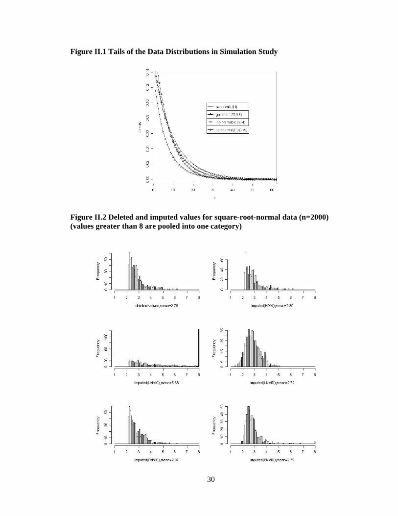
Figure II.1 Tails of the Data Distributions in Simulation Study
Figure II.2 Deleted and imputed values for square-root-normal data (n=2000) (values greater than 8 are pooled into one category)
30

Figure II.4 Deleted and imputed values for 1995 Chinese household income project, rural data (values greater than 60,000 are pooled into one category)
Figure II.3 Deleted and imputed values for 1995 Chinese household income project, urban data (values greater than 85,000 are pooled into one category)
31

32
Figure II.5 Standardized regression coefficients, after versus before imputation. 1995 Chinese household income project, urban data. (Top row, HDMI, with cutoff points being 90, 80, 60, 40 percentiles, from left to right. Middle row, LNMID. Bottom row, PNMIC. Line: y = x)

Appendix II.1: PMI method for log-normal model and power-transformed normal model For X from log-normal 2( , )μ σ distribution, 2log( ) ~ ( , )Y X N μ σ= . If X is from the
power-transformed normal ( 2, ,μ σ λ ) distribution with 0λ ≠ ,
( ) 21 / ~ ( , )Y X Nλ λ μ σ= − . To apply the PMI method we estimate λ by its ML
estimate λ̂ using the widely available routine box.cox.powers( ) in R (see Fox 2006), and
then assume ( )ˆ 2ˆ1 / ~ ( , )Y X Nλ λ μ σ= − . (A more principled approach would also
simulate λ from its posterior distribution).
Given data from the1( ,... )nY y y= 2( , )N μ σ distribution, the posterior distribution
of parameters is as follows,
2
22
1
( 1)| ~n
n SYσχ −
− , where 2
1
1 (1
n
ii
S yn =
=− ∑ 2)y− (IIA1)
and
2| , ~ ( , / )Y N y nμ σ σ 2 . (IIA2)
We draw parameters * *2,μ σ from their posterior distribution and then draw deleted
values for normal data from the predictive distribution
. (IIA3) * * *2del ~ ( , | log )IY N Y yμ σ >
We then transform the draws of normal data back to log-normal and power-transformed
normal data:
log-normal: * *del delexp( )X Y= (IIA4)
power-transformed normal: ˆ* *del del
ˆ(X Yλ λ 1)= + (IIA5)
33

Appendix II.2: EM algorithm for log-normal model If X is log-normal( 2,μ σ ), then log( )Y X= is 2( , )N μ σ and .
Let be a random sample from
2' ( ) exp( / 2)E Xμ μ= = +σ
1( ,... )nY y y= 2( , )N μ σ , and suppose iy is treated as
missing if and only if iy c> , where c is a known censored value. Without loss of
generality, we assume iy is observed for 1, 2,...,i r= and missing for . The
complete-data likelihood is
1,...,i r n= +
2 2 2 2
1 1
( , | ) exp{ log /(2 ) /(2 ) / }n n
i ii i
L Y n y n y 2μ σ σ σ μ σ μ= =
∝ − − − +∑ ∑ σ .
(IIA6)
The complete-data sufficient statistics are
2
1 1( ) ( , )
n n
i ii i
S Y y y= =
= ∑ ∑ . (IIA7)
We write , where denotes the observed values and denotes the
missing values. Given parameter estimates , the ( )th iteration of EM
method is as follows:
obs del( ,Y Y Y= )
)t
obsY misY
( ) ( ) ( )( ,t tθ μ σ= 1t +
E-step:
( ) 2 ( )2 ( ) 2 ( )2
( 1) ( )0 obs
1
( )
1 11
( ) /(2 ) ( ) /(2 )
( )2 ( )21
( | , )
( | , )
1 1( ) e e2 2
t t t t
nt t
ii
r nt
i i ii i r
ry y
i t tc ci
s E y Y
y E y y c
y n r y dy dyμ σ μ σ
θ
θ
πσ πσ
+
=
= = +
−∞ ∞− − − −
=
=
= + >
⎛ ⎞= + − ⎜ ⎟
⎝ ⎠
∑
∑ ∑
∑ ∫ ∫
(IIA8)
34

( ) 2 ( )2 ( ) 2 ( )2
( 1) 2 ( )1 obs
11
2 2 ( ) /(2 ) ( ) /(2 )
( )2 ( )2
( | , )
1 1( ) e et t t t
nt t
ii
ry y
i t tc c
s E y Y
y n r y dy dyμ σ μ σ
θ+
=
1 2 2i πσ πσ
−∞ ∞− − − −
=
⎛ ⎞= + − ⎜ ⎟
∑
∑ ∫ ∫= ⎝ ⎠
(IIA9)
M-step:
(IIA10)
Once the sequence of
( 1) ( 1)0
( 1)2 ( 1) ( 1)2 21 0
/
/ /
t t
t t t
s n
s n s n
μ
σ
+ +
+ + +
=
= −
( )tθ has converged to a stable value ( ,μ σ% % ), we calculate the ML
estimate of 'μ as
. (IIA11) 24̂ ' exp( / 2)θ μ μ σ= = +% % %
35

Chapter III Extensions of Multiple Imputation Methods as Disclosure Control
Procedure for Multivariate Data
Abstract
Multiple imputation (MI) has been proved to be effective statistical disclosure control
(SDC) method for data with extreme values. Previous studies demonstrate MI methods
provide better inference of the publicly-released data than the commonly-used top-coding
procedure, while maintaining good SDC properties. We propose stratified and regression-
based extensions of these MI methods for multivariate analysis. We show in simulation
studies that our proposed methods work well in preserving relationship within
multivariate data and provide results from regression analysis close to those obtained
before imputation. We illustrate the methods on data from the 1995 Chinese household
income project.
Keywords: confidentiality, disclosure protection, multiple imputation
III.1 Introduction
Statistical disclosure control (SDC) is a class of procedures that deliberately alter data
collected by statistical agencies before release to the public, to prevent the identity of
survey respondents from being revealed. These methods have increased in importance,
with the extensive use of computers and the internet. The goal of SDC methods is to
reduce the risk of disclosure to acceptable levels, while releasing a dataset that provides
36

as much useful information as possible for researchers. One aspect of this is the ability to
draw valid statistical inferences from the altered data.
A great number of confidentiality concerns are raised by extreme values of
variable. For example, in surveys that include income, extremely high income values are
considered to have the potential to reveal the identity of respondents. Top-coding is a
simple SDC procedure in this situation. A “top-code” is defined, and values greater than
the top-code are recoded to that value. Top-coding is easy to implement, and widely used
in surveys.
We have proposed multiple imputation as an alternative to top-coding for
disclosure limitation (An and Little, 2007a). Data values greater than a cutoff point,
which is chosen to be smaller than the top-code, are deleted. These values are replaced
either by random draws from the set of deleted values (the hot-deck procedure), or by
draws from the posterior predictive distribution based on the imputation model (the
Bayesian procedure). The imputation process is repeated several times and the imputed
datasets are then released to the public. Inferences can be calculated with MI combining
rules (Reiter 2003). An and Little (2007a) show that MI methods provide better
inferences than top-coding, while maintaining good SDC properties.
An and Little (2007a) focus mainly on inference for a population mean, yet most
uses of publicly-released data files concern multivariate analysis. That paper also shows
that in situation where the outcome variable is subject to top-coding, failure of the
imputation model to condition on covariates leads to attenuation of relationships between
outcome and covariates. The goal of this article is to propose extensions of MI methods
37
for multivariate data that preserve the associations between variables and yield valid
estimate of regression coefficients.
We propose two extensions, stratified MI and regression-based MI. For the
stratified method, we calculate predicted values of the outcome variable from regression
model and create strata based on the predicted values. We then apply previous MI
methods within each stratum to fill in deleted values. The regression method is based on a
regression of the outcome on the set of fully observed covariates. We condition the
predictive distribution of the deleted values on covariates for imputation, by including the
covariates in the mean function of the outcome.
We compare estimates of regression coefficients from our methods with estimates
from the original data, and with two estimates from top-coded data. The first treats the
top-coded values as the true values. The second treats values greater than top-code as
censored, and bases inferences on a model fitted to the censored data.
The rest of this paper is organized as follows. Section III.2 presents our SDC
approaches and extensions. Section III.3 describes corresponding methods of inference
for regression coefficients. Section III.4 describes a simulation study to evaluate the
approaches in Section III.3, and Section III.5 applies the methods to data from the 1995
Chinese household income project. Section III.6 concludes with discussion.
III.2 Methods of statistical disclosure control
Let Y denote a survey variable (e.g. income) and suppose that values of Y greater than a
particular value are considered too sensitive for release to the public. Let X denote a
set of fully observed variables that are not subject to disclosure limitation methods. Our
goal is to develop SDC methods that preserve relationship between Y and the X’s .
Ty
38

III.2.1 Previous SDC methods
For inference about the marginal mean of Y without covariates, An and Little (2007a)
distinguish the following methods.
(A) Top-coding. Treat as a top-code value, that is, replace values of Y greater than
by . The resulting sample is referred to as “top-coded”.
Ty
Ty Ty
(B) Hot-deck MI (HDMI). Choose a value smaller than . Delete the values of Y
greater than and replace them with random draws from the set of deleted values. We
choose to achieve a mixing of sensitive and non-sensitive values. We refer to
as the cutoff point.
Iy Ty
Iy
TI yy < Iy
(C) Parametric MI (PMI). The HDMI method is arguably limited from the point of
view of SDC, since actual sensitive data values are released. The PMI methods address
this concern by releasing data simulated from a parametric model. As with HDMI, we
delete values greater than . Fit a statistical model (e.g. lognormal model) to the data.
Parameters are drawn from their posterior distribution under the assumed model, and
deleted values are imputed with draws from their predictive distribution.
Iy
Write the complete data as ret del( , )Y Y Y= , where denotes the retained values
and denotes the deleted values beyond the cut-off. We consider two versions of PMI,
labeled as PMIC and PMID. For PMIC, we draw the parameter
retY
delY
φ of the model for the
data Y from its posterior distribution given the complete data Y. For PMID, we apply the
parametric model to the deleted data , and draw delY φ from its posterior distribution
given . For inference about a population mean, PMID is less efficient than PMIC
because it models the deleted data and fails to exploit fully the information in Y when
delY
39

drawing values of parameters. However, modeling the deleted data only as in PMID
provides useful robustness to model misspecification, since the model is being fitted to
the data that are being deleted. See An and Little (2007a) for more details.
III.2.2 Extensions of MI methods for multivariate data
The methods in Section III.2.1 do not condition on covariates and potentially attenuate
relationships between the variables. We propose methods that condition imputation of
deleted values on the observed X’s. From this section we refer to (Y, X) as the complete
data prior to SDC; and refer to the deleted values of Y and their corresponding values of
X’s as the deleted data.
(a) Stratified HDMI method. Assign the deleted data into strata based on predicted
values of Y from regression of Y on X. Apply HDMI within each stratum to impute for
deleted values.
(b) Stratified PMI method. Again create strata based on predicted values of Y. For
PMIC methods, we stratify the complete data. For PMID methods, we stratify the deleted
data as in (a). We then apply statistical models to the values of Y in each stratum and
impute deleted values with draws from predictive distribution.
(c) Regression PMI method. Instead of fitting models to the marginal distribution of
variable Y, we include covariates in the mean function of the model for Y. We draw
parameters from their posterior distribution under the assumed model, and draw deleted
values from predictive distribution. We fit the model to the complete data (for PMIC
method) and the deleted data (for PMID). See Appendix III.1 for details for log-normal
and power-transformed-normal model.
40

(d) Regression MI method based on top-coded data set. Fit a statistical (e.g., log-
normal) model to the data with values of Y below the top-code. We obtain draws of
parameter using a Gibbs sampler (Little and Rubin, 2002), and impute deleted values
with draws from predictive distribution.
The stratified and regression versions of HDMI and PMI methods in (a)-(c) will
be later referred to as “S*” and “R*” methods, respectively.
III.3 Methods of inference
We study the properties of these SDC methods for inferences about regression coefficient
with Y being outcome (or covariate). The regression model is fitted to the dataset before
and after imputation. The following estimates and associated standard errors are
considered:
(1) Before Deletion (BD) – the estimate of regression coefficient calculated from original
data prior to SDC. This estimate is used as a benchmark for comparing SDC methods.
(2) Top-coding (TC) – the estimate of regression coefficient from the top-coded sample,
where we treat the top-coded values as the true values.
The standard errors for methods BD and TC are computed by the bootstrap, with
B = 100 bootstrap samples.
(3) Log-normal MI from top-coded data (LNMIT) – the estimates from D imputed
datasets, where we draw imputations for values beyond the top-code from the posterior
distributions with a log-normal model fitted to the top-coded data. The MI estimate is
calculated using the standard MI combining rule for missing data (Little and Rubin,
2002). In particular, the MI estimate of variance from this method is calculated as
DDBWVarT MIMI /)1()ˆ( +∗+== θ . (1)
41
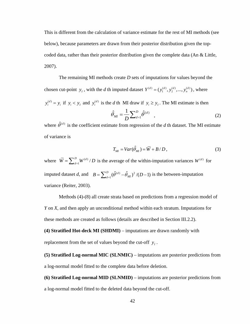
This is different from the calculation of variance estimate for the rest of MI methods (see
below), because parameters are drawn from their posterior distribution given the top-
coded data, rather than their posterior distribution given the complete data (An & Little,
2007).
The remaining MI methods create D sets of imputations for values beyond the
chosen cut-point Iy , with the d th imputed dataset , where
if
( ) ( ) ( ) ( )1 2( , ,..., )d d d d
nY y y y=
( )di iy y= i Iy y< and is the d th MI draw if ( )d
iy i Iy y≥ . The MI estimate is then
, (2) ∑ θ̂
where ( )ˆ dθ is the coefficient estimate from regression of the d th dataset. The MI estimate
of variance is
==
D
dd
MI D 1)(1θ̂
ˆ( ) /MI MIT Var W Bθ= = + D , (3)
where ( )1
/D dd
W W=
=∑ D is the average of the within-imputation variances for
imputed dataset d, and is the between-imputation
variance (Reiter, 2003).
( )dW
∑ =−−=
D
d MId DB
12)( )1/()ˆˆ( θθ
Methods (4)-(8) all create strata based on predictions from a regression model of
Y on X, and then apply an unconditional method within each stratum. Imputations for
these methods are created as follows (details are described in Section III.2.2).
(4) Stratified Hot-deck MI (SHDMI) – imputations are drawn randomly with
replacement from the set of values beyond the cut-off Iy .
(5) Stratified Log-normal MIC (SLNMIC) – imputations are posterior predictions from
a log-normal model fitted to the complete data before deletion.
(6) Stratified Log-normal MID (SLNMID) – imputations are posterior predictions from
a log-normal model fitted to the deleted data beyond the cut-off.
42

(7) Stratified Power-normal MIC (SPNMIC) – imputations are posterior predictions
from a power-transformed normal model fitted to the full data before deletion. For
convenience the power transformation is estimated by ML, and parameters are drawn
from the full-data posterior distribution treating the power transformation as known.
(8) Stratified Power-normal MID (SPNMID) – imputations are posterior predictions
from the power-normal model, fitted to the deleted data beyond the cut-off.
Methods (9)-(12) are based on predictions from a regression model that includes
the covariates linearly in the mean structure of the model. Details of these methods are
described in Appendix III.1. Imputations for these methods are created in a similar
manner as their counterparts of stratified methods.
(9) Regression Log-normal MIC (RLNMIC)
(10) Regression Log-normal MID (RLNMID)
(11) Regression Power-normal MIC (RPNMIC)
(12) Regression Power-normal MID (RPNMID)
III.4 Simulation study
A simulation study was carried out to evaluate and compare the SDC methods in Section
III.3. We computed estimates of regression coefficients, the corresponding variances and
confidence intervals from the imputed datasets, and compared them with those calculated
from the original dataset prior to SDC.
III.4.1 Study design
Datasets were generated from the following two distributions. For each distribution, we
simulated data where the covariates are strongly or weakly correlated.
Data distribution 1:
43

When X1 and X2 are strongly correlated,
X1 ~ Normal (0, 1); X2|X1 ~ Normal (0.9*X1, 0.19); X3|X1, X2 ~ Normal (0.2*X1+X2,
0.16)
When X1 and X2 are weakly correlated,
X1 ~ Normal (0, 1); X2|X1 ~ Normal (0.3*X1, 0.91); X3|X1, X2 ~ Normal (0.2*X1+X2,
0.13)
Data distribution 2:
When X1 and X2 are strongly correlated,
X1~ Normal (0, 1); X2|X1~ Normal (0.9*X1, 0.19); X3|X1, X2~ Normal (X1+X2, 0.42)
When X1 and X2 are weakly correlated,
X1 ~ Normal (0,1); X2|X1 ~ Normal (0.3*X1, 0.91); X3|X1, X2 ~ Normal (X1+X2, 0.29)
Here X3 is logarithm of variable Y subject to disclosure control. For regression
purpose we treated X3 as dependent variable and X1 and X2 as independent variables.
Data distributions 1 and 2 have different proportions of contribution from the two
covariates. To assess sensitivity of SDC methods to model misspecification, we also
investigate situation where X3 was generated from a different distribution with the same
mean function.
For each simulated dataset, we applied top-coding, stratified and regression MI
methods to impute the deleted values of Y and performed linear regression on imputed
dataset. We then calculated estimates of regression coefficients, the corresponding
variances, 95% confidence intervals (CI’s) based on normal approximation and the
coverage of confidence intervals. For comparison, we also considered MI methods that
failed to condition on the covariates (referred to as unconditional methods).
44

In our simulations we chose the 95th percentile of the population distribution as
the top-code value . Denote by the number of sensitive sample values greater
than . We studied two alternative values for the cutoff point :
Ty Sn
Ty Iy 90Iy , the value with
larger values in the sample, and 2 Sn 80Iy , the value with larger values in the sample.
These values correspond approximately to the 90th and 80th percentiles of the distribution,
and for this reason we label the version of a method * that uses cutoff
4 Sn
90Iy “*90” and the
version that uses cutoff 80Iy “*80”.
Clearly the disclosure risk is reduced by increasing the fraction of non-sensitive
values that are imputed. A simple measure of the risk of disclosure is the proportion of
multiple-imputed values beyond the top-code value Ty . For all the MI methods, this is
approximately 50% when the cutoff point is 90Iy , and approximately 25% when the
cutoff point is 80Iy .
III.4.2 Results
Unless specified otherwise, the results from simulation are based on 500 data sets
generated from data distribution 1, with sample sizes 2000. We set B = 100 for the
number of bootstrap samples. For MI methods, we created D = 5 imputed datasets for
values beyond 90Iy . For stratified MI methods, we created strata with stratum size around
40.
Table III.1 and III.2 show estimates of regression coefficients for X1, X2, and the
intercept term, when X1 and X2 are strongly correlated and weakly correlated,
respectively. Results are calculated from top-coding, unconditional and conditional MI
methods. TC in Table III.1 underestimates the regression coefficients for both covariates.
45

The estimates of the coefficient of X2 have larger bias and less coverage, since top-
coding the outcome results in greater attenuation of the relationship between outcome and
covariate when they are more associated. TC also provides underestimates of the
intercept term with poor coverage, suggesting inadequate estimation of the marginal
mean of X3. When X1 and X2 are weakly correlated, TC estimates for X1 and X2 have
reduced coverage. The impact is more severe with X2, suggesting that the attenuation
effect has been reduced by the high correlation between the covariates.
All unconditional MI methods behave similarly and underestimate coefficients of
both covariates, with larger bias for estimate of the coefficient of X2. Though most of the
estimates have acceptable confidence coverage (except that estimates of the coefficient of
X2 have low coverage when X1 and X2 are not strongly associated), it is worth noticing
that these estimates have a 20-30% increase (or 30-40% in some cases) in CI width
compared with BD. As a result, some over coverage is observed for the intercept term.
Stratified HDMI produces negligible bias and close to nominal coverage for all
three estimates. SLNMID and SPNMID methods also work quite well, with small
increases in RMSE and CI width compared to BD estimates. Estimates from SLNMIC
and SPNMIC methods have good confidence coverage, though they tend to be more
biased and less efficient than those from stratified HD and PMID methods. There is a
minor increase in bias for estimate of the coefficient of X2 from all MI methods, as for
the TC method. Results in Table III.2 show some loss of efficiency in the estimate of
coefficient of X2. We observe that increasing number of strata results in better inference,
especially for the S-PMIC method (result not shown).
46

All regression PMI methods yield inferences close to those before deletion.
LNMIT works almost as well as the R-PMI methods; and appears to be a reasonable
approach to the analysis of the top-coded dataset. LNMIT and RPNMID have slightly
less efficient estimates of the coefficient of X2 when X1 and X2 are weakly correlated.
Regression PMI methods (especially RLNMIC and RPNMIC) are more efficient than
stratified PMI methods, and produce less bias for the coefficient of X2. Overall, estimates
from stratified and regression methods are less biased and more efficient than those from
unconditional MI methods.
When the data are from the second distribution with X1 and X2 contributing
evenly in regression (Table III.3 and III.4), we observe similar properties of stratified and
regression methods as from the first data distribution, except that here estimates of the
coefficients of X1 and X2 have very similar inferential properties.
For the smaller sample size of 500 (Table III.5 and III.6), estimates from the
stratified methods have larger RMSE and relative CI width. Regression methods also
result in larger RMSE and RPNMID shows some increases in CI width; but in general
they produce better inferences than stratified methods.
When changing the cutoff point from 90Iy to 80Iy (Table III.7 and III.8), stratified
HDMI almost has same performance. SLNMID and SPNMID methods have minor
increases in bias, RMSE and CI width. More substantial increases are seen with SLNMIC
and SPNMIC. In situation where there is low correlation between two covariates, these
two methods do not provide full coverage. Results from all regression methods remain
somewhat unchanged, whereas RPNMID yields less efficient estimates. Unlike stratified
and regression methods, lowering cutoff point for unconditional MI methods results in
47
larger bias and RMSE, and major increase in CI width. Estimates of coefficient of X1 still
have satisfactory coverage, while for intercept some over coverage occurs. With X2 the
estimates of the coefficient have low coverage, which gets worse when X1 and X2 are
weakly correlated.
Table III.9 and III.10 display results in situation where X3 was generated from an
exponential distribution instead of normal distribution, to evaluate method performance
when model is mis-specified for the outcome. TC again underestimates the regression
coefficients for X1 and X2, yielding serious bias and low coverage for estimate of the
coefficient of X2. Estimate of intercept is even more biased and has worse coverage. All
TC estimates have 20% less of CI width than BD estimates. Unconditional HDMI and
LNMID, as well as PN methods for strongly correlated covariates, yield satisfactory
results, though they are in general more biased and less efficient than stratified and
regression methods. Among stratified MI methods, SHDMI and SLNMID have the best
performances. They work consistently well and produce estimates with minimal bias and
good coverage. SLNMIC method has very similar properties as TC, though it is
somewhat less biased and has better confidence coverage. Stratified PNMIC and PNMID
methods have larger bias than SLNMID, otherwise they work quite well. For regression
methods, estimates from LNMIT have sizable bias and reduced CI width, and have
acceptable coverage except for the intercept term. RLNMIC has even worse performance
than LNMIT, and has lower coverage for estimate of the coefficient of X2, as X2
associates more with the outcome. RLNMID works best with inferences close to before
deletion, and seems to be robust to model misspecification of X3. RPNMIC is more
biased than RLNMID but also works well. RPNMID produces satisfactory results for X1
48

and X2, whereas for intercept it is more biased and does not provide full coverage (even
unconditional PNMID method has better results in this case). In a word, regression based
MI methods are no better than the stratified versions of these methods.
In summary, stratified HDMI and PMID methods perform well overall. Stratified
PMIC methods are less satisfactory in some situations, indicating that stratification on
deleted data is adequate and efficient. Among regression methods, RLNMID has the best
performance. RPNMIC also works quite well. RPNMID produces satisfactory inferences
under correct model; and with incorrect model it yields biased estimates for the marginal
mean of the outcome. LNMIT only imputes values beyond top-code, which may be one
reason for its close performance as other MI methods. LNMIT and S/RLNMIC methods
are all sensitive to model misspecification. LNMIT has less impact with tail of
distribution being mis-specified, due to the fact that it conditions only on values below
top-code. This could also explain why LNMIT works almost as well as other R-PMI
methods under correct model, as fewer values are being imputed. On the other hand,
LNMIT presents higher risk of disclosure than other MI methods.
III.4.3 Results from regression of X1 on X2 and imputed X3
We further investigate the impact of SDC methods on regressions where the sensitive
variable subject to top-coding is a covariate. We applied previous SDC approaches to
impute for deleted values of X3 as before. We then regressed X1 on X2 and X3 and
computed coefficients from regression.
Simulation setting is the same as described in Section III.4.1. Table III.11 and
III.12 present results from situation where X1 is strongly and weakly correlated with X2,
respectively. TC results in biased estimates with poor confidence coverage.
49

Unconditional MI methods provide poor results for coefficients of X2 and X3. Estimates
from these methods have serious bias and much lower coverage than TC estimates.
Table III.11 shows SHDMI has minimal bias and confidence coverage close to
before deletion. SLNMID and SPNMID methods work nearly as well. SLNMIC produces
good estimate for intercept; and estimates of the coefficients of X2 and X3 have less CI
width and less coverage than BD, yet they behave better than TC estimates. SPNMIC
yields estimate with similar inferences to those from the SLNMIC method. When X1 and
X2 are weakly correlated (Table III.12), SHDMI maintains same properties except for
some minor increase in bias and RMSE. All estimates of the coefficients of X2 and X3
from stratified PMI methods have larger bias and lower coverage than in Table III.11;
especially with MIC methods.
All regression methods yield estimates with good inferences. Result from LNMIT
method is close to those from RLNMIC and RPNMIC methods. RPNMID has slightly
higher bias especially when correlation between X1 and X2 is weak. Overall, these
methods have reduced bias and RMSE comparing with their stratified counterparts. We
conclude that in situations where imputations are carried out on a covariate, regression
MI methods are obviously advantageous to stratified methods for inference about
regression coefficient; and they definitely outdo unconditional methods.
III.5 Application
We also consider the properties of the SDC methods on a multiple regression, estimated
on a subset of the urban data in the 1995 Chinese Household Income Project (Riskin et
al.2000). This project was designed to measure the personal income distribution in the
People’s Republic of China in 1995. Income information on both household and
50

individual were recorded for rural and urban areas. This dataset is a good example to
assess the effectiveness of the various SDC methods, since SDC was not applied to the
released dataset.
III.5.1 Data analysis
Our sample included 10,752 individuals and 10 variables, with the logarithm of income
treated as the dependent variable. The covariates involved were age, gender, marital
status, education level, occupation, work environment, work intensity, years of work
experience and logarithm of hours worked per week. To simplify the analysis, we only
investigate the situation where the covariates are complete.
We applied the stratified and regression HDMI and PMI methods to the data as
previously described and computed estimates of regression coefficients from imputed
dataset. As in simulation study, we also calculated estimates from the unconditional MI
methods (i.e., imputation does not condition on covariates) for comparison.
III.5.2 Results
We plot estimates of the standardized regression coefficients after imputation against
those from the original dataset (Fig. III.1-III.3). We choose HDMI, LNMID and PNMIC
as representations of the MI methods and use the 90th, 80th, 60th and 40th percentiles of the
outcome variable as cutoff points, to assess the effect of increasingly severe imputation.
Figure III.1 shows the result from unconditional imputation. We observe that
with 90Iy , the regression coefficients from the imputed dataset are quite close to those
from the dataset before imputation; and imputation with 80Iy also has a minor effect on
the coefficients. Lower cutoff points result in larger deviation from original coefficients.
Figure III.2 displays result from stratified MI methods. Imputations with 90Iy , as well
51

as 80Iy , yield regression coefficients very close to those from original data. Coefficients
computed from RLNMID and RPNMIC (Figure III.3) present very similar properties as
in Figure III.2. Comparing to Figure III.1, coefficients from Figure III.2 and Figure III.3
show some minor improvements, especially with lower cutoff point. But overall, they are
not much different from those in Figure III.1.
This particular case is similar to the scenario from simulation study where the
outcome and covariates have low correlation (as the case with X1). We conclude that in
such situation, the unconditional MI methods are robust to the failure of the imputation
model to condition on covariates. Lowering cutoff points results in larger deviation from
original coefficients, leading to greater attenuation of the relationship between outcome
and covariates. This impact is less severe with stratified and regression methods.
III.6 Discussion
When applying the MI method to multivariate data, we should condition the predictive
distribution of the deleted values on observed covariates. Our previous assessment of
inferences for regression coefficients from unconditional MI methods confirms that
failure to condition on covariates leads to an attenuation of relationships between
outcome and covariates. In simple situation where a small set of categorical covariates
associate strongly with the outcome, it may suffice to apply the MI methods within strata
defined by these covariates. We base our stratified method on this idea and consider more
general application with presence of continuous covariates. Since we are interested in
preserving association between outcome and covariates, we define strata with the
predicted values from regression.
52

Of our proposed methods, the stratified methods are easy to apply and involve
only a limited amount of computation. The regression-based methods are potentially
more efficient, but a bit more complicated computationally. As for method performance,
these stratified and regression extensions of MI methods are in general superior to top-
coding and unconditional MI methods for inference about regression coefficient. It is
clear that treating the top-coded data as the observed data yields bias, the size of which
depends on the fraction of cases top-coded and the extremity of the top-code. The
LNMIT method based on top-coded data works quite well under correct model, but is
vulnerable to model misspecification. Regression LNMID has the best performance and
yields results close to before deletion. SHDMI, SLNMID and RPNMIC methods also
produce good inferences. RPNMID method works well except when estimating the
marginal mean of outcome, with mis-specified model. SPNMIC and SPNMID methods
work well when the outcome is subject to SDC. When the imputations are performed on a
covariate, they (SPNMIC in particular) yield less satisfactory results. Both stratified and
regression versions of LNMIC method are vulnerable to misspecification.
We chose the log-normal and power normal models to illustrate parametric MI,
since they are commonly used to model skewed data; they are not universal, and the MI
approach could applied by the data producer with other models that are more suitable for
the data at hand.
We have confined attention here to inferences from top-coding and MI methods;
other alternatives to top-coding are also of interest. One such alternative is to add random
noise (e.g., normal noise as in Fuller 1993) to the values beyond top-code. This method
may yield satisfactory (if less efficient) inferences for the mean, but noise with
53

substantial variance needs to be added to yield reductions of disclosure risk comparable
to those of MI, and adding such noise potentially distorts the distribution. Also custom
adjustments are needed for inferences about other parameters, such as regression
coefficients. Note that if multiple imputes are created by adding noise to the true value,
the average of these imputations converges to the true value as the number of imputations
increases, an undesirable property from the perspective of disclosure protection. Our MI
methods do not have this property: the average of the MI imputed values converges to the
conditional mean of the predictive distribution, not the true deleted value. Thus
increasing the number of MI’s improves efficiency of inferences without compromising
gains in disclosure protection. This is a major attraction of MI as an SDC method.
54

55
Acknowledgments
This work was supported by National Institute of Child and Human Development grant
(P01 HD045753). The authors thank Trivellore Raghunathan, Michael Elliott, and Myron
Gutmann for useful comments.
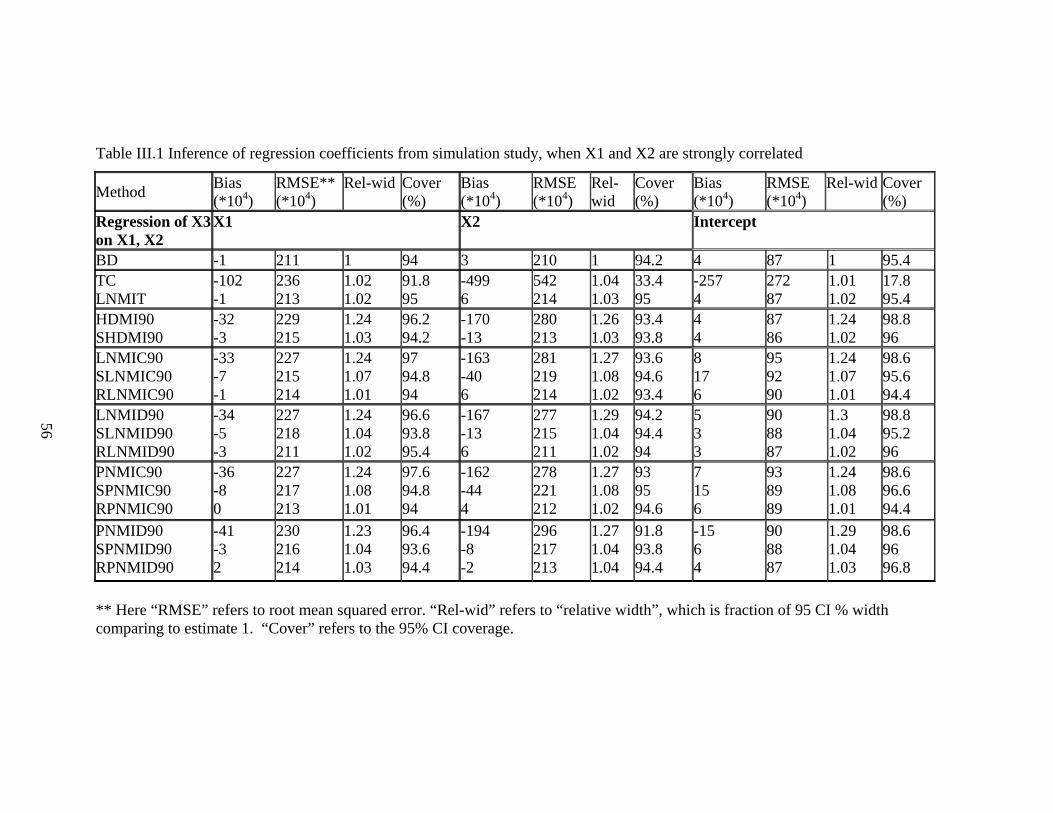
Table III.1 Inference of regression coefficients from simulation study, when X1 and X2 are strongly correlated
Method Bias (*104)
RMSE** (*104)
Rel-wid Cover (%)
Bias (*104)
RMSE (*104)
Rel-wid
Cover (%)
Bias (*104)
RMSE (*104)
Rel-wid Cover (%)
Regression of X3 on X1, X2
X1 X2 Intercept
BD -1 211 1 94 3 210 1 94.2 4 87 1 95.4 TC LNMIT
-102 -1
236 213
1.02 1.02
91.8 95
-499 6
542 214
1.04 1.03
33.4 95
-257 4
272 87
1.01 1.02
17.8 95.4
HDMI90 SHDMI90
-32 -3
229 215
1.24 1.03
96.2 94.2
-170 -13
280 213
1.26 1.03
93.4 93.8
4 4
87 86
1.24 1.02
98.8 96
LNMIC90 SLNMIC90 RLNMIC90
-33 -7 -1
227 215 214
1.24 1.07 1.01
97 94.8 94
-163 -40 6
281 219 214
1.27 1.08 1.02
93.6 94.6 93.4
8 17 6
95 92 90
1.24 1.07 1.01
98.6 95.6 94.4
LNMID90 SLNMID90 RLNMID90
-34 -5 -3
227 218 211
1.24 1.04 1.02
96.6 93.8 95.4
-167 -13 6
277 215 211
1.29 1.04 1.02
94.2 94.4 94
5 3 3
90 88 87
1.3 1.04 1.02
98.8 95.2 96
PNMIC90 SPNMIC90 RPNMIC90
-36 -8 0
227 217 213
1.24 1.08 1.01
97.6 94.8 94
-162 -44 4
278 221 212
1.27 1.08 1.02
93 95 94.6
7 15 6
93 89 89
1.24 1.08 1.01
98.6 96.6 94.4
PNMID90 SPNMID90 RPNMID90
-41 -3 2
230 216 214
1.23 1.04 1.03
96.4 93.6 94.4
-194 -8 -2
296 217 213
1.27 1.04 1.04
91.8 93.8 94.4
-15 6 4
90 88 87
1.29 1.04 1.03
98.6 96 96.8
56
** Here “RMSE” refers to root mean squared error. “Rel-wid” refers to “relative width”, which is fraction of 95 CI % width comparing to estimate 1. “Cover” refers to the 95% CI coverage.

Table III.2 Inference of regression coefficients from simulation study, when X1 and X2 are weakly correlated
Method Bias (*104)
RMSE (*104)
Rel-wid Cover (%)
Bias (*104)
RMSE (*104)
Rel-wid
Cover (%)
Bias (*104)
RMSE (*104)
Rel-wid Cover (%)
Regression of X3 on X1, X2
X1 X2 Intercept
BD 2 86 1 96.2 1 91 1 93.8 4 79 1 94.8 TC LNMIT
-100 1
133 87
1.02 1.02
78.2 94.8
-498 1
509 93
1.13 1.09
0.2 93.8
-225 4
240 80
1.01 1.03
19.8 95.4
HDMI90 SHDMI90
-34 -1
96 86
1.22 1.02
96.4 95.4
-166 -13
193 91
1.33 1.05
74.8 94
4 4
79 79
1.22 1.03
98.8 95.8
LNMIC90 SLNMIC90 RLNMIC90
-33 -6 2
96 86 87
1.23 1.07 1.01
96.8 96.6 94
-158 -37 4
197 97 92
1.36 1.11 1.04
73.2 94 93
9 17 6
85 81 80
1.24 1.08 1.01
97.2 96.6 95.4
LNMID90 SLNMID90 RLNMID90
-33 -1 1
96 86 86
1.23 1.03 1.02
96.4 94.6 94.8
-163 -10 -0
192 93 89
1.46 1.08 1.05
78 94.4 94.2
5 5 3
82 80 80
1.29 1.04 1.02
97.8 96 95.8
PNMIC90 SPNMIC90 RPNMIC90
-33 -8 3
97 86 87
1.22 1.07 1.01
97 96.4 94.2
-161 -44 4
195 101 92
1.35 1.13 1.04
72.2 93.4 92.4
7 14 6
83 81 80
1.23 1.08 1.01
98.4 96.2 95.2
PNMID90 SPNMID90 RPNMID90
-39 -1 2
100 86 87
1.22 1.04 1.03
95.6 95.2 95.6
-193 -11 1
218 93 92
1.43 1.08 1.08
69.6 93.6 93.8
-13 5 5
83 80 80
1.28 1.04 1.03
98.4 96.2 95.8
57
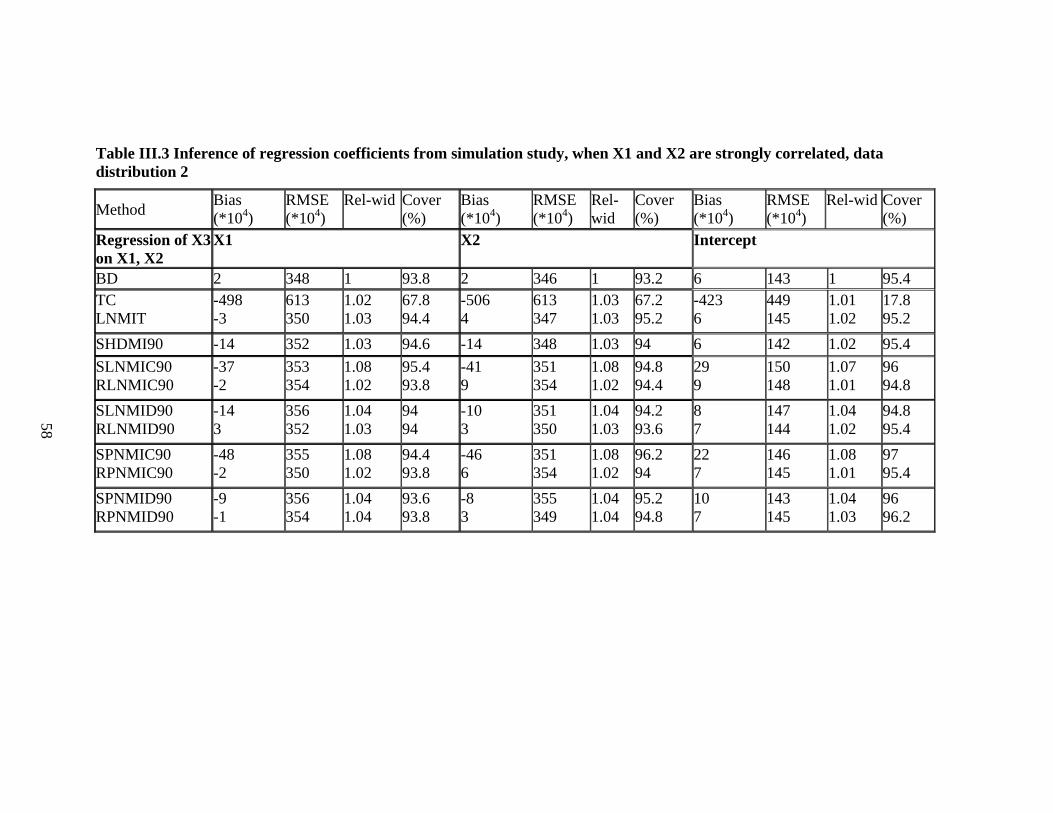
Table III.3 Inference of regression coefficients from simulation study, when X1 and X2 are strongly correlated, data distribution 2
Method Bias (*104)
RMSE (*104)
Rel-wid Cover (%)
Bias (*104)
RMSE (*104)
Rel-wid
Cover (%)
Bias (*104)
RMSE (*104)
Rel-wid Cover (%)
Regression of X3 on X1, X2
X1 X2 Intercept
BD 2 348 1 93.8 2 346 1 93.2 6 143 1 95.4 TC LNMIT
-498 -3
613 350
1.02 1.03
67.8 94.4
-506 4
613 347
1.03 1.03
67.2 95.2
-423 6
449 145
1.01 1.02
17.8 95.2
SHDMI90 -14 352 1.03 94.6 -14 348 1.03 94 6 142 1.02 95.4 SLNMIC90 RLNMIC90
-37 -2
353 354
1.08 1.02
95.4 93.8
-41 9
351 354
1.08 1.02
94.8 94.4
29 9
150 148
1.07 1.01
96 94.8
SLNMID90 RLNMID90
-14 3
356 352
1.04 1.03
94 94
-10 3
351 350
1.04 1.03
94.2 93.6
8 7
147 144
1.04 1.02
94.8 95.4
SPNMIC90 RPNMIC90
-48 -2
355 350
1.08 1.02
94.4 93.8
-46 6
351 354
1.08 1.02
96.2 94
22 7
146 145
1.08 1.01
97 95.4
SPNMID90 RPNMID90
-9 -1
356 354
1.04 1.04
93.6 93.8
-8 3
355 349
1.04 1.04
95.2 94.8
10 7
143 145
1.04 1.03
96 96.2
58

Table III.4 Inference of regression coefficients from simulation study, when X1 and X2 are weakly correlated, data distribution 2
Method Bias (*104)
RMSE (*104)
Rel-wid Cover (%)
Bias (*104)
RMSE (*104)
Rel-wid
Cover (%)
Bias (*104)
RMSE (*104)
Rel-wid Cover (%)
Regression of X3 on X1, X2
X1 X2 Intercept
BD 3 128 1 95 2 131 1 93.6 6 118 1 95.6 TC LNMIT
-502 1
521 133
1.08 1.05
5.4 94
-499 2
517 134
1.08 1.05
4 95.2
-349 6
370 119
1.02 1.03
18.2 95.6
SHDMI90 -13 133 1.03 94.4 -11 137 1.04 93.8 6 118 1.03 95.8 SLNMIC90 RLNMIC90
-38 3
138 135
1.08 1.02
94.8 93.4
-38 5
139 137
1.09 1.02
95.2 93.2
25 8
122 123
1.08 1.02
96.4 94.6
SLNMID90 RLNMID90
-16 3
135 128
1.05 1.03
94.8 95.4
-14 1
138 132
1.06 1.03
94.4 93.4
4 9
120 118
1.04 1.02
95.4 95.8
SPNMIC90 RPNMIC90
-47 5
141 131
1.09 1.02
95.6 94
-46 5
144 134
1.1 1.02
94 93.2
19 9
123 119
1.09 1.02
95.6 95.4
SPNMID90 RPNMID90
-9 2
134 133
1.05 1.05
95.4 95.8
-6 -1
137 134
1.06 1.06
93.6 95.2
9 6
120 119
1.05 1.04
96.4 96
59

Table III.5 Inference of regression coefficients from simulation study, when X1 and X2 are strongly correlated, n = 500
Method Bias (*104)
RMSE (*104)
Rel-wid Cover (%)
Bias (*104)
RMSE (*104)
Rel-wid
Cover (%)
Bias (*104)
RMSE (*104)
Rel-wid Cover (%)
Regression of X3 on X1, X2
X1 X2 Intercept
BD -3 425 1 93.2 -0 422 1 92.6 4 185 1 93.2 TC LNMIT
-89 -2
437 429
1.02 1.03
92.8 93.8
-513 1
674 432
1.04 1.04
76.4 94
-255 4
320 186
1.02 1.03
68.4 93.4
SHDMI90 -2 447 1.04 92.4 -16 447 1.04 93.6 3 185 1.04 93.8 SLNMIC90 RLNMIC90
2 -7
444 457
1.15 1.03
95.8 90.8
-34 12
444 450
1.16 1.03
95.8 91.6
71 10
197 191
1.16 1.03
94.8 92.8
SLNMID90 RLNMID90
-3 -3
458 441
1.13 1.05
95.2 93
-20 -1
455 437
1.14 1.05
95.2 94.2
-0 3
190 188
1.14 1.04
95.2 94.4
SPNMIC90 RPNMIC90
-3 -6
439 452
1.16 1.03
96.2 91.8
-31 3
440 447
1.17 1.04
95.4 92.4
71 5
194 190
1.17 1.03
94.8 93
SPNMID90 RPNMID90
-0 -2
452 440
1.13 1.07
95 93.8
-24 18
455 442
1.14 1.08
95.4 93
-4 12
190 190
1.14 1.07
94.4 95.2
60

Table III.6 Inference of regression coefficients from simulation study, when X1 and X2 are weakly correlated, n = 500
Method Bias (*104)
RMSE (*104)
Rel-wid Cover (%)
Bias (*104)
RMSE (*104)
Rel-wid
Cover (%)
Bias (*104)
RMSE (*104)
Rel-wid Cover (%)
Regression of X3 on X1, X2
X1 X2 Intercept
BD -1 176 1 93 -1 176 1 93 4 168 1 93.6 TC LNMIT
-107 -0
206 180
1.02 1.03
89.8 94.8
-500 5
538 188
1.14 1.09
25 93.4
-233 6
291 168
1.02 1.03
70.2 93.6
SHDMI90 -6 185 1.03 92.6 -18 185 1.05 93.4 1 168 1.03 94 SLNMIC90 RLNMIC90
-10 -0
183 189
1.15 1.02
96 93.2
-33 8
197 190
1.2 1.05
94.6 91
60 10
184 173
1.15 1.02
95 93
SLNMID90 RLNMID90
-2 -2
188 178
1.13 1.04
94.2 94
-12 -1
198 187
1.2 1.07
93.8 93.2
4 4
175 168
1.14 1.04
94.8 93.6
SPNMIC90 RPNMIC90
-7 1
185 186
1.16 1.02
95.6 93
-27 9
190 188
1.22 1.05
96 92.8
66 11
184 172
1.17 1.03
95.2 94.2
SPNMID90 RPNMID90
-4 -0
188 184
1.12 1.07
94.4 94.6
-20 15
200 196
1.2 1.13
94 93.6
-2 10
171 169
1.13 1.07
96.8 95
61

Table III.7 Inference of regression coefficients from simulation study with cutoff point 80Iy , when X1 and X2 are strongly correlated
Method Bias (*104)
RMSE (*104)
Rel-wid Cover (%)
Bias (*104)
RMSE (*104)
Rel-wid
Cover (%)
Bias (*104)
RMSE (*104)
Rel-wid Cover (%)
Regression of X3 on X1, X2
X1 X2 Intercept
BD -1 211 1 94 3 210 1 94.2 4 87 1 95.4 TC LNMIT
-102 -1
236 213
1.02 1.02
91.8 95
-499 2
542 213
1.04 1.03
33.4 94.4
-257 4
272 86
1.01 1.02
17.8 95.4
HDMI80 SHDMI80
-90 -5
263 224
1.53 1.04
98.2 93.4
-434 -10
498 221
1.55 1.04
77.6 93.8
5 5
88 88
1.52 1.03
99.6 95.8
LNMIC80 SLNMIC80 RLNMIC80
-90 -15 -4
261 218 219
1.53 1.12 1.02
97.4 96 93.6
-429 -88 6
495 233 217
1.56 1.13 1.03
77.4 93.4 94.2
9 18 5
105 90 92
1.58 1.13 1.02
98.6 97 93.6
LNMID80 SLNMID80 RLNMID80
-89 -6 -0
261 222 216
1.53 1.05 1.04
97.4 94.6 93.6
-439 -7 1
501 224 215
1.58 1.06 1.04
77.8 93.2 93.6
4 5 3
96 90 87
1.67 1.06 1.03
99.8 95.4 94.8
PNMIC80 SPNMIC80 RPNMIC80
-91 -15 -2
263 217 218
1.53 1.12 1.02
97 96 93.4
-431 -86 5
497 229 217
1.57 1.13 1.03
77.4 96.6 93.2
8 20 5
100 91 88
1.58 1.13 1.02
99.4 96.8 94.6
PNMID80 SPNMID80 RPNMID80
-98 -4 -1
260 220 216
1.53 1.05 1.06
97.6 94.4 94
-472 -3 19
528 220 222
1.58 1.06 1.07
72.2 94.6 93.6
-28 8 9
100 91 90
1.66 1.06 1.06
99.2 95.4 96
62

Table III.8 Inference of regression coefficients from simulation study with cutoff point 80Iy , when X1 and X2 are weakly correlated
Method Bias (*104)
RMSE (*104)
Rel-wid Cover (%)
Bias (*104)
RMSE (*104)
Rel-wid
Cover (%)
Bias (*104)
RMSE (*104)
Rel-wid Cover (%)
Regression of X3 on X1, X2
X1 X2 Intercept
BD 2 86 1 96.2 1 91 1 93.8 4 79 1 94.8 TC LNMIT
-100 1
133 86
1.02 1.02
78.2 95.2
-498 1
509 92
1.13 1.09
0.2 93.4
-225 4
240 80
1.01 1.03
19.8 96
HDMI80 SHDMI80
-85 -2
131 87
1.5 1.03
94.4 94.4
-435 -14
447 92
1.6 1.06
6.6 94.2
4 4
80 80
1.5 1.03
99.6 96
LNMIC80 SLNMIC80 RLNMIC80
-85 -16 2
133 88 88
1.5 1.12 1.02
95.4 96.4 94.8
-429 -86 5
448 127 95
1.69 1.17 1.05
14 86.8 93.2
9 17 7
94 84 82
1.55 1.13 1.03
99.2 96.6 95.2
LNMID80 SLNMID80 RLNMID80
-88 -1 3
133 88 88
1.5 1.05 1.03
95.4 94.8 94
-440 -15 1
454 94 94
1.8 1.11 1.07
14.4 95 94
1 4 4
88 82 80
1.64 1.06 1.04
99.6 95.6 95.4
PNMIC80 SPNMIC80 RPNMIC80
-84 -17 3
133 89 88
1.49 1.12 1.02
94.8 96.6 94
-431 -83 2
447 123 93
1.7 1.18 1.05
11.6 89 93.6
7 19 6
89 83 83
1.55 1.13 1.02
99.6 96.6 94.2
PNMID80 SPNMID80 RPNMID80
-93 -1 3
137 88 89
1.5 1.05 1.06
93.6 94.2 95.4
-469 -7 12
483 92 94
1.79 1.11 1.13
10.2 94.4 94.8
-22 7 8
91 82 82
1.63 1.07 1.06
99 95.8 95.2
63

Table III.9 Inference of regression coefficients from simulation study from incorrect model, when X1 and X2 are strongly correlated
Method Bias (*104)
RMSE (*104)
Rel-wid Cover (%)
Bias (*104)
RMSE (*104)
Rel-wid
Cover (%)
Bias (*104)
RMSE (*104)
Rel-wid Cover (%)
Regression of X3 on X1, X2
X1 X2 Intercept
BD 37 3229 1 94.6 -93 3224 1 93.8 -69 1412 1 92.8 TC LNMIT
-393 -326
2703 3748
0.82 0.88
93 94.2
-1964 -1527
3308 4020
0.82 0.88
86.4 92.6
-3369 -3116
3637 3610
0.82 0.88
18.2 49.6
HDMI90 SHDMI90
-238 -57
3124 3383
1.08 1.02
96 92.6
-876 -61
3233 3380
1.08 1.02
95.4 94.4
-80 -67
1427 1424
1.08 1.02
95.4 94.8
LNMIC90 SLNMIC90 RLNMIC90
-463 -391 -440
2691 2750 3654
0.84 0.86 0.84
93.6 93.6 93.8
-2148 -1796 -2012
3405 3268 4154
0.84 0.86 0.84
86 88.8 89
-3584 -2967 -4561
3830 3275 4903
0.84 0.87 0.84
15.2 30.6 18.6
LNMID90 SLNMID90 RLNMID90
-270 -72 45
3074 3380 4324
1.08 1.03 1.03
96.6 92.6 95
-830 -48 -88
3186 3335 4321
1.08 1.03 1.03
96.2 94.2 94.4
-81 -62 -103
1434 1470 1874
1.14 1.05 1.03
95.6 92.8 94
PNMIC90 SPNMIC90 RPNMIC90
-273 -218 -187
3005 3088 4158
1.07 1.04 1.02
96.8 95.4 94.8
-1059 -874 -935
3196 3187 4258
1.07 1.03 1.02
95.4 95 93.6
-624 -275 -546
1593 1510 2007
1.07 1.04 1.02
92.2 93.2 92.4
PNMID90 SPNMID90 RPNMID90
-271 -89 -151
3043 3290 4014
1.03 1 0.97
96 93.2 95.2
-1073 -286 -720
3216 3271 4062
1.02 0.99 0.97
95 94.2 94.6
-654 -523 -1135
1582 1508 2157
1.06 1 0.97
91.6 92.2 88.6
64
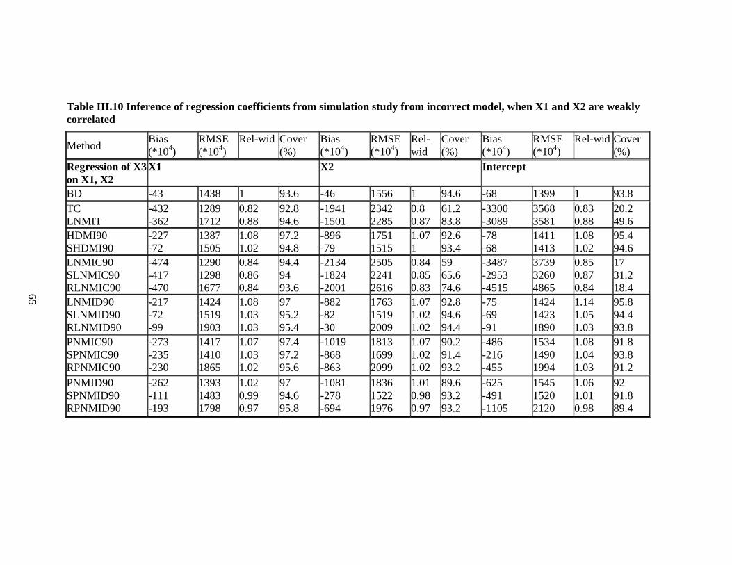
Table III.10 Inference of regression coefficients from simulation study from incorrect model, when X1 and X2 are weakly correlated
Method Bias (*104)
RMSE (*104)
Rel-wid Cover (%)
Bias (*104)
RMSE (*104)
Rel-wid
Cover (%)
Bias (*104)
RMSE (*104)
Rel-wid Cover (%)
Regression of X3 on X1, X2
X1 X2 Intercept
BD -43 1438 1 93.6 -46 1556 1 94.6 -68 1399 1 93.8 TC LNMIT
-432 -362
1289 1712
0.82 0.88
92.8 94.6
-1941 -1501
2342 2285
0.8 0.87
61.2 83.8
-3300 -3089
3568 3581
0.83 0.88
20.2 49.6
HDMI90 SHDMI90
-227 -72
1387 1505
1.08 1.02
97.2 94.8
-896 -79
1751 1515
1.07 1
92.6 93.4
-78 -68
1411 1413
1.08 1.02
95.4 94.6
LNMIC90 SLNMIC90 RLNMIC90
-474 -417 -470
1290 1298 1677
0.84 0.86 0.84
94.4 94 93.6
-2134 -1824 -2001
2505 2241 2616
0.84 0.85 0.83
59 65.6 74.6
-3487 -2953 -4515
3739 3260 4865
0.85 0.87 0.84
17 31.2 18.4
LNMID90 SLNMID90 RLNMID90
-217 -72 -99
1424 1519 1903
1.08 1.03 1.03
97 95.2 95.4
-882 -82 -30
1763 1519 2009
1.07 1.02 1.02
92.8 94.6 94.4
-75 -69 -91
1424 1423 1890
1.14 1.05 1.03
95.8 94.4 93.8
PNMIC90 SPNMIC90 RPNMIC90
-273 -235 -230
1417 1410 1865
1.07 1.03 1.02
97.4 97.2 95.6
-1019 -868 -863
1813 1699 2099
1.07 1.02 1.02
90.2 91.4 93.2
-486 -216 -455
1534 1490 1994
1.08 1.04 1.03
91.8 93.8 91.2
PNMID90 SPNMID90 RPNMID90
-262 -111 -193
1393 1483 1798
1.02 0.99 0.97
97 94.6 95.8
-1081 -278 -694
1836 1522 1976
1.01 0.98 0.97
89.6 93.2 93.2
-625 -491 -1105
1545 1520 2120
1.06 1.01 0.98
92 91.8 89.4
65

Table III.11 Inference of regression coefficients from simulation study, when X1 and X2 are strongly correlated
Method Bias (*104)
RMSE (*104)
Rel-wid Cover (%)
Bias (*104)
RMSE (*104)
Rel-wid
Cover (%)
Bias (*104)
RMSE (*104)
Rel-wid Cover (%)
Regression of X1 on X2, X3
X2 X3 Intercept
BD 2 295 1 94.2 1 239 1 93.6 0 94 1 96.2 TC LNMIT
331 3
438 298
0.97 1.02
78.8 94.6
-169 0
294 241
1 1.02
89.6 94.8
56 -0
110 93
1 1.01
90.4 96
HDMI90 SHDMI90
684 75
733 305
0.97 1
30.2 93.6
-547 -58
586 245
0.98 1
32.4 94.2
-0 -1
93 93
1.01 1.01
96.2 96
LNMIC90 SLNMIC90 RLNMIC90
685 290 2
730 401 301
0.97 0.97 1.01
30.6 84.4 94.2
-548 -234 1
584 324 244
0.98 0.97 1.01
32.8 82.8 94.8
-1 -3 -1
93 93 94
1.01 1.01 1.01
95.8 96.2 95.8
LNMID90 SLNMID90 RLNMID90
689 107 10
737 314 295
0.97 1 1.02
28 92.4 94.6
-551 -84 -5
590 252 238
0.98 1 1.02
31.4 93.4 95.2
-0 -0 -0
93 93 93
1.02 1.01 1.01
96.2 96 95.8
PNMIC90 SPNMIC90 RPNMIC90
689 307 1
735 415 302
0.97 0.97 1.01
27.8 82.4 94.2
-551 -245 1
589 335 243
0.98 0.97 1.01
31.4 82.2 95.2
-1 -3 -1
93 93 93
1.01 1.01 1.01
96.4 96.2 96
PNMID90 SPNMID90 RPNMID90
681 112 58
730 312 297
1 1 1.01
34 92.8 95
-538 -90 -46
580 253 241
1.02 1 1.02
36.8 93 94.8
3 -1 -0
93 93 94
1.02 1.01 1.01
96 96.2 96.2
66

Table III.12 Inference of regression coefficients from simulation study, when X1 and X2 are weakly correlated
Method Bias (*104)
RMSE (*104)
Rel-wid Cover (%)
Bias (*104)
RMSE (*104)
Rel-wid
Cover (%)
Bias (*104)
RMSE (*104)
Rel-wid Cover (%)
Regression of X1 on X2, X3
X2 X3 Intercept
BD -26 511 1 95.2 19 451 1 95.6 4 182 1 95.2 TC LNMIT
1128 -23
1245 513
1.04 1.02
48.8 96.2
-548 16
726 452
1.05 1.02
79.8 95.6
250 3
311 184
1.01 1.01
74.4 95.8
HDMI90 SHDMI90
2611 226
2667 558
1.06 1
0.4 95
-2110 -203
2163 492
1.1 1.01
1.4 94.2
4 4
182 183
1.05 1.01
96.8 95.2
LNMIC90 SLNMIC90 RLNMIC90
2631 991 -25
2678 1111 510
1.06 0.99 1.01
0.2 55.2 96
-2135 -901 16
2179 1004 450
1.1 1.02 1.01
0.6 50 95.8
-1 -9 1
185 183 184
1.05 1.02 1.01
96.8 95.6 95
LNMID90 SLNMID90 RLNMID90
2621 326 -4
2678 607 514
1.06 1.01 1.01
0.2 91.4 96
-2122 -300 0
2176 542 453
1.08 1.01 1.01
1 91.4 95.8
2 2 4
184 182 184
1.06 1.01 1.01
96.6 95.6 95.6
PNMIC90 SPNMIC90 RPNMIC90
2618 1061 -27
2668 1180 518
1.06 0.99 1.01
0.2 48.4 96
-2122 -961 17
2168 1064 457
1.1 1.02 1.01
1 45.2 96.2
1 -6 1
183 184 184
1.05 1.02 1.01
96.4 95.6 94.6
PNMID90 SPNMID90 RPNMID90
2592 363 188
2649 638 560
1.16 1.02 1.03
0.4 89.8 94
-2066 -335 -182
2122 569 502
1.24 1.02 1.03
3 90.4 95.2
19 3 3
184 184 183
1.06 1.02 1.01
97.4 95.6 95.4
67

Figure III.1 Standardized regression coefficients, after versus before unconditional imputation. 1995 Chinese household income project, urban data. (Top row, HDMI, with cutoff points being 90, 80, 60, 40 percentiles, from left to right. Middle row, LNMID. Bottom row, PNMIC. Line: y = x)
68

Figure III.2 Standardized regression coefficients, after versus before stratified imputation. 1995 Chinese household income project, urban data. (Top row, SHDMI, with cutoff points being 90, 80, 60, 40 percentiles, from left to right. Middle row, SLNMID. Bottom row, SPNMIC. Line: y = x)
69

70
Figure III.3 Standardized regression coefficients, after versus before regression-based imputation. 1995 Chinese household income project, urban data. (Top row, RLNMID, with cutoff points being 90, 80, 60, 40 percentiles, from left to right. Bottom row, RPNMIC. Line: y = x)

Appendix III.1: Regression-based parametric MI methods for log-normal model and power-transformed normal model As described in the paper, let Y denote the variable subject to disclosure limitation and X
denote the covariate matrix. Let Z be a normal variable transformed from Y. To be
specific, if Y is from a log-normal distribution, let )log(YZ = . If Y is from a power-
transformed-normal distribution with 0≠λ , let . Here we estimateλλ /)1( −= YZ λ by its
ML estimate using the widely available routine boxcox ( ) in R (see Fox(2006)) and
then assume that .
λ̂
λλ ˆ/)1( ˆ−= YZ
Let Xi denote the vector of covariates for the i th observation,
),(~| 2σβ∑ j jijii xNXZ . (IIIA1)
Write , without loss of generality, assume ),( delret ZZZ = ),...,( 1 rret zzZ = and
. ),...,( 1 nrdel zzZ +=
For PMIC method, the posterior distribution of parameters is
2
22 ˆ)(~|*
pn
pnZ−
−χ
σσ (IIIA2)
and
)*)(,ˆ(~,*|* 212 σβσβ −XXMVNZ T , (IIIA3)
where
ZXXX TT 1)(ˆ −=β (IIIA4)
pn
xzn
j jiji
−
−=∑ ∑1
22
)ˆ(ˆ
βσ . (IIIA5)
71

We draw parameters *β and from their posterior distribution and draw deleted values
for normal data from the predictive distribution
2*σ
2 nrizZxNXZ Ij jijiidel ,...,1),|*,*(~|* )( +=>∑ σβ , (IIIA6)
where for log-normal distribution; or for power-normal
distribution.
)log( II yz = λλ /)1( −= II yz
We then transform the draws of normal data back to log-normal,
)*exp(* )()( idelidel ZY = , (IIIA7)
and power-transformed normal data,
λ λˆ)()( )1*ˆ(* += idelidel ZY . (IIIA8)
For PMID method the calculations are quite similar as above, except that the model is
fitted to the deleted data instead of the complete data.
72

Chapter IV A Multiple Imputation Approach to Disclosure Limitation for High-age
Individuals in Longitudinal Studies
Abstract Disclosure limitation is an important consideration in the release of public use data sets.
It is particularly challenging for longitudinal data sets, since information about an
individual accumulates with repeated measures over time. Despite the challenges,
research on disclosure limitation methods for longitudinal data has been very limited. We
consider here problems created by high ages in cohort studies. Because of the risk of
disclosure, ages of very old respondents can often not be released; in particular this is a
specific stipulation of the Health Insurance Portability and Accountability Act (HIPAA)
for the release of health data for individuals. Top-coding of individuals beyond a certain
age is a standard way of dealing with this issue, and it may be adequate for cross-
sectional data, given that a modest number of cases are likely to be affected. However,
this approach has severe limitations in longitudinal studies, when individuals have been
in the study for many years. We propose and evaluate an alternative to top-coding for this
situation based on multiple imputation (MI). This MI method is applied to a survival
analysis of simulated data and data from the Charleston Heart Study (CHS), and is shown
to work well in preserving the relationship between hazard and covariates.
73

Keywords: confidentiality, disclosure protection, longitudinal data, multiple imputation,
survival analysis
IV.1 Introduction
Statistical disclosure control is a class of procedures that deliberately alter data collected
by statistical agencies before release to the public, to prevent the identity of survey
respondents from being revealed. These methods have increased in importance, with the
extensive use of computers and the internet. The goal of SDC methods is to reduce the
risk of disclosure to acceptable levels, while releasing a dataset that provides as much
useful information as possible for researchers. One aspect of this is the ability to draw
valid statistical inferences from the altered data.
Top-coding is a simple and common SDC method that seeks to prevent disclosure
on the basis of extreme values of a variable, by censoring values above a pre-chosen
“top-code”. For example, in surveys that include income, extremely high income values
are considered to be sensitive and to have the potential to reveal the identity of
respondents. By recoding income values greater than a selected “top-code” value to that
value, respondents with very high income have reduced risk of disclosure.
It is left to the analyst to decide how top-coded data are analyzed. One approach is
to categorize the variable so that top-coded cases all fall in one category – this is sensible,
but precludes analyses that treat the variable as continuous. Another approach is to ignore
the fact of top-coding and treat the top-coded values as the truth. This method is
straightforward, but clearly the data distribution is distorted and biased estimates will be
obtained. A better method is to treat the extreme values as censored. Under an assumed
statistical model, maximum likelihood (ML) estimates can be obtained using algorithms
74

such as the Expectation-Maximization (EM) algorithm (Dempster, Laird and Rubin,
1977). This method is model-based, and should yield good inferences if the model is
correctly specified. But we expect this method to be quite sensitive to model
misspecification, especially when the upper tail of the assumed distribution differs
markedly from that of the true distribution. The data users can also apply an imputation
method to the top-coded dataset and fill in the censored values. A limitation is that the
imputed data fail to reflect imputation uncertainty, and imputations are sensitive to
assumptions about the right tail of the distribution. An and Little (2007a) propose an
alternative to top-coding based on multiple imputation (MI), which allows valid
inferences to be created based on applying multiple imputation combining rules described
by Reiter (2003), while preserving the SDC benefits of top-coding; for other discussions
of MI in the disclosure control setting, see Little (1993); Rubin (1993); Little, Liu and
Raghunathan (2004); Reiter(2005a, 2005b). The methods in An and Little (2007a) are
extended to handle covariate information in An and Little (2007b).
We propose here MI for disclosure control in the context of the treatment of age
in longitudinal data sets. Because of the risk of disclosure, ages of very old respondents
can often not be released; in particular this is a specific stipulation of HIPAA regulations
for the release of health data for individuals. Top-coding of individuals beyond a certain
age (say 80) is a standard way of dealing with this issue, and it may be adequate for
cross-sectional data, since the number of cases affected may be modest. However, this
approach has severe limitations in longitudinal studies, when individuals have been in the
study for many years; for example, consider an individual in a 40-year longitudinal study,
who enters the study at age 42 at time t and is still in the study at age 82 at time t+40. The
75

age at time t+40 cannot simply be replaced by a top code of 80, since age at time t+40
can be inferred by simply adding 40 to the age at time t. A strict application of top-coding
would replace all individuals aged 40 or older at time t by a top code of 40, but this
strategy seriously limits the ability to do longitudinal analysis, particularly survival
analyses where chronological age is a key variable of interest. In particular, since age at
entry is a marker for cohorts, differences in outcomes between cohorts aged 40 or greater
at entry can no longer be estimated, since these cohorts are all top-coded to the same
value.
This problem arises in the Charleston Heart Study (Nietert et al., 2000), a
longitudinal study that collects data over 40 years (1960-2000). The study was originally
conducted to understand the natural aging process in a community-based cohort. The data
include baseline characteristics such as age, race, gender, occupation, education; as well
as death information for respondents. For longitudinal data from this study to be included
in the data archive at the University of Michigan, individual ages beyond age 80 cannot
be disclosed because of HIPAA regulation, given the geographic specificity of the
respondents. Also, given the longitudinal nature of the data, a top-coding approach would
need to be applied to all individuals aged 40 or older in 1960, which has the limitation
discussed above.
The goal of this research is to develop MI methods that suffice to limit disclosure
risk and preserve the relationship between hazard and covariates in survival analysis. We
propose a non-parametric MI method, specifically a stratified hot-deck procedure, where
we create strata and draw deleted ages with replacement from each stratum. Our method
76

concerns MI of two age variables – entry age and final age (age at death or age at last
contact).
To assess the proposed method, we apply a proportional hazard (PH) model to the
multiply-imputed datasets, calculate estimates of regression coefficients for putative risk
factors, and compare these estimates, and corresponding estimates from top-coded data,
with estimates from the PH model applied to the original data prior to SDC. We also
present simulation studies where data are simulated according to a known survival model,
and inferences for parameters of this model are compared with the true values.
The rest of this paper is organized as follows. Section IV.2 presents our SDC
approaches for longitudinal data and describes corresponding methods of inference for
regression coefficients. Section IV.3 describes a simulation study to evaluate the
approaches in Section IV.2, and Section IV.4 applies the methods to CHS data. Section
IV.5 gives discussion and future work.
IV.2 Methods
IV.2.1 SDC methods for longitudinal data
An and Little (2007a) propose SDC methods for a single variable with extreme values. In
this paper, we investigate a more complicated situation with longitudinal data, where two
age variables are subject to top-coding.
Let Yend denote participants’ age at the end of study (referred to as final age) and
Ystart denote their entry age. Let C be the censoring indicator. Let L represent the length of
study and S denote time of survival. Individuals with are treated as censored (C =
1), and otherwise died (C = 0). We consider individuals with values of Yend greater than a
particular value
LS ≥
0y to be at risk of disclosure, and refer to these individuals as sensitive
77

cases. Thus values of Yend and Ystart of the sensitive cases are treated as sensitive values.
We consider the following approaches to SDC.
(a) Top-coding. Replace values of Yend greater than 0y by 0y and replace values of Ystart
greater than 0y L− by 0y L− . The resulting dataset is referred to as “top-coded” data.
(b) Hot-deck MI (HDMI). Classify sensitive and non-sensitive values into strata, to be
defined below. Then delete the values of Yend , Ystart, and C for sensitive cases and replace
them with random draws from the set of deleted values in the same stratum. Our stratified
HDMI method is similar to the approach described in An and Little (2007b), where we
assign the deleted data into strata based on predicted values of either age variables from
regression on other variables, and apply HDMI within each stratum to impute deleted
values. The following choices of strata are considered here:
(i) HD1. Strata are defined by predicted values of the logarithm of hazard computed from
the proportional hazard model.
(ii) HD2. Strata are defined by predicted values of entry-age, from the regression of
entry-age on other variables involved.
(iii) HD3. We develop a two-way stratification, where strata are defined by both
predicted values of the logarithm of hazard, and predicted values of entry-age.
(iv) HD4. Stratification depends on the value of C. For individuals that are censored,
strata are defined by predicted values of entry-age; and for those not censored, strata are
defined by both predicted values of the logarithm of hazard and predicted values of entry-
age.
(v) HD5. We directly apply HDMI method without stratification, for comparison with the
stratified methods.
78

Note that for methods HD1 – HD3, we delete values of Yend, Ystart, and C of
sensitive cases and jointly impute these values. HD4 retains values of C and imputes Yend
and Ystart only.
It is worth mentioning that for above stratified methods, we perform regression
only on the deleted cases to obtain predicted values. We also consider an alternative way
of stratification, where we perform regression on the complete data, and then stratify the
sensitive cases for imputation. Results from these methods are briefly described in
Section IV.3.
IV.2.2 Methods of inference
We consider the properties of the SDC methods for inferences about the regression
coefficient, where a PH model is fitted to the dataset before and after imputation. The
following estimates and associated standard errors are considered:
(1) Before Deletion (BD) – the estimates of regression coefficients calculated from
original data prior to SDC, used as a benchmark for comparing SDC methods.
(2) Top-coding (TC) – the estimates of regression coefficients calculated from top-coded
dataset.
The standard errors for methods (1) and (2) are computed by the bootstrap.
The five remaining methods HD1 – HD5 are as described in Section IV.2.1,
yielding D MI datasets. The MI estimate is calculated as
, (1)
where ( )ˆ dθ is the parameter estimate from d th data set. The MI estimate of variance is
ˆ( ) /MI MIT Var W Bθ= = + D , (2)
∑ ==
D
dd
MI D 1)(ˆ1 θθ̂
79

where ( )1
/D dd
W W=
=∑ D is the average of the within-imputation variances for
imputed data set d, and is the between-imputation
variance. The formula (2) differs from the original MI formula for missing data (where B
is multiplied by a factor (D+1)/D, see e.g. Little and Rubin, 2002, p86), for reasons
discussed in Reiter (2003).
( )dW
∑ =−−=
D
d MId DB
12)( )1/()ˆˆ( θθ
IV.3 Simulation study
A simulation study was carried out to evaluate the top-coding and MI methods in Section
IV.2. We computed estimates of regression coefficients, their corresponding variances
and confidence intervals from the imputed and top-coded datasets, and compared them
with those calculated from the original dataset prior to SDC.
IV.3.1 Study design
For simplicity we simulated survival data with just two binary covariates, representing
gender (male and female) and entry age (say 30 - 40 and 40 - 50). Datasets were
simulated from multinomial distribution in four categories defined by these variables.
Values of entry-age were generated from uniform distribution. Survival times (in years)
were generated from piece-wise exponential distributions with hazard rates specified in
Table IV.1 and IV.2. An individual was treated as censored if (s)he survived more than
40 years from age at entry. We investigated the following three scenarios.
Scenario I Distributions of entry age do not depend on gender; both male and female
have same entry-age distributions.
Scenario II Distributions of entry age are different for males and females.
Scenario III Distributions of entry age are the same for males and females, and there is
interaction between entry age and gender.
80

In this study we considered individuals with final age greater than or equal to 75
years to be at risk of disclosure, and refer to these individuals as sensitive cases. For each
simulated dataset, we applied the stratified HDMI methods to both final age and entry
age variables for sensitive cases as described in Section IV.2. We also applied the top-
coding method, with top-code being 75 for final age and 35 for entry age (as the length of
study is 40 years). We then calculated estimates of regression coefficients from the PH
model, the corresponding variances of the estimates, as well as 95% confidence intervals
(CI’s) based on normal approximation, and the confidence coverage of these intervals.
IV.3.2 Results
Simulation results are based on 500 datasets of sample size 2000. We set the number of
bootstraps B to be 100 for calculating standard errors of BD and TC estimates; and create
D = 5 imputed datasets. For stratified HDMI methods, we create strata with stratum size
around 25.
Table IV.3 presents results from scenario I, where distributions of entry-age are
the same for male and female. TC yields estimate of regression coefficient with serious
bias and RMSE, and zero confidence coverage for the entry-age variable. As for gender,
TC estimate has relatively better properties, yet it still has sizable bias and low coverage.
All stratified HDMI methods produce quite satisfactory results for the entry-age variable,
with negligible bias and confidence coverage close to before deletion. HD5 also work
well in terms of bias and coverage, but it is somewhat less efficient than the stratified HD
methods. HD4 method works best for gender variable, yielding estimate of regression
coefficient with minimal bias and good confidence coverage. Estimates from other HD
methods are also acceptable, though they are in general more biased and have less
81

coverage. When male and female have different entry-age distributions as in scenario II
(Table IV.4), most methods behave similarly as in the first scenario, except that HD3
yields larger bias, RMSE and less coverage for estimate of the regression coefficient of
gender. In fact, it has even worse results than TC method.
Table IV.5 displays results from scenario III, where there is interaction between
the age and gender variables. TC yields estimates with considerable bias and poor
coverage for regression coefficients of age, gender and the interaction between these two
variables. Among stratified HD methods, HD4 has the best performance and yields
estimates with good inferences for both variables and the age-gender interaction. HD2
also has satisfactory results for all three terms, though it is more biased than HD4.
Estimates from HD1 and HD3 methods have similar properties as from HD2, except that
they have less sufficient coverage for the interaction term. Estimates from HD5 have
larger bias and less confidence coverage than those from the stratified HD methods.
We also applied the alternative stratified method described in Section IV.2.1,
where we obtained predicted values from regression on the complete data, and then
stratified the sensitive cases for imputation. Estimates from these methods (not shown)
are more biased and have less confidence coverage compared to the methods above. This
suggests that when a regression model is fitted to the data that are being deleted, it makes
the method more robust to model mis-specification and yield better result (see Section
IV.5 for more discussion).
In summary, HD4 performs best under all circumstances. Other stratified HD
methods yield estimates of regression coefficient with good inferential properties for the
entry-age variable. These methods also provide satisfactory results for gender, except for
82

HD3 in scenario II. With presence of interaction between age and gender, estimates for
the interaction term from HD1 and HD3 methods do not have sufficient coverage. HD5
tends to be slightly less efficient than the stratified HD methods, but it works surprisingly
well in the first two scenarios, indicating stratification may not be necessary in such data
setting. For more complicated situation (scenario III), it yields biased estimates with low
confidence coverage.
IV.4 Application in Charleston Heart Study data
We chose a subset of the CHS data and studied the relationship between hazard rate and
certain risk factors. Since an intact data file prior to disclosure control was available to
us, the effectiveness of our SDC methods can be readily assessed.
IV.4.1 Primary data analysis
After deletion of missing values and recoding on some variables, our sample included
1344 individuals, of which 303 survived the study. The variables involved were entry-
age, final-age, censoring indicator, race/gender, education level, current cigarette
smoking status, history of myocardial infraction (MI), history of diabetes, history of
hypertension, electro-cardiographic interpretation (EKG), living place between age 20 to
65 and body mass index (BMI). For the PH regression model, final-age instead of
survival time was treated as the time-scale variable.
To examine effects of our chosen risk factors, we applied the PH model to the
dataset prior to SDC. Table IV.6 displays results from the regression. All factors have
significant effect on participant’s hazard ratio except BMI and entry-age (overall).
Comparing to individuals that enter the study between 35 and 40 years old, those with
entry-age greater than 50 have about a 30% increase in risk of death. White females tend
83

to have 34% less of risk than white males. Achieving education after high school reduces
hazard by 30% comparing to non-high school education. Smoking cigarette increases
death risk by 76%. Participants with definite history of myocardial infraction have twice
the risk of death as those without a history. History of diabetes as well as EKG problems
increases the hazard by over 50%, while history of hypertension increases risk of death
by 17%. Rural residents have 25 % less of hazard than urban residents. Most of these
coefficients are in the expected direction.
IV.4.2 Results from SDC methods
As described earlier, variables subject to disclosure limitation are entry-age and final-age
variables. Respondents with final-age greater than or equal to 80 years are considered to
be sensitive cases, which intuitively leads to top-code values of 40 for entry-age and 80
for final-age. For this dataset, top-coding the age variables has great impact on the
analysis, since the entry-age variable is recoded into only two categories (40 or below
40), in contrast to the five categories for entry-age in the original data. We applied HDMI
methods to the data and computed estimates of regression coefficient from a PH model.
Table IV.7 shows results from original, top-coded and imputed datasets based on
500 replications. Predictably, TC considerably alters the relationship between hazard and
covariates and yields estimates of the regression coefficients with serious bias, especially
for the entry-age variable. Of the stratified HDMI methods, HD3 and HD4 yield
estimates of coefficients of entry-age close to those from BD. HD1 provides better
estimates of regression coefficients than other methods for the gender variable. For the
rest of covariates, none of the stratified HD methods seems to have an obvious advantage,
with HD2 being slightly inferior. HD5 has less satisfactory results, though it still yields
84

better estimates than TC for some covariates. Overall, the stratified HD methods all work
better than top-coding in preserving the relationship between risk of death and the
covariates on this dataset.
IV.5 Discussion
Longitudinal data raise particular confidential concerns with potentially extensive
longitudinal information gathered over time. We consider a specific application
concerning disclosure risk caused by some participants attaining high ages because of
prolonged participation in a longitudinal study, as in the Charleston Heart Study. One of
the authors (McNally) has the responsibility to prepare a public use version of this data
set at the Data Archive at Michigan that meets HIPAA regulations. As discussed earlier,
the standard approach of top-coding age has severe limitations in this longitudinal setting,
especially for survival analyses with age being a key variable of interest. We develop MI-
based SDC methods for this particular data setting. Similar to the methods in An and
Little (2007b), our proposed MI methods are based on stratification, with strata defined
by the predicted values of the age variables from a regression model.
Regarding the longitudinal nature of dataset in this study, we have focused on
inference about regression coefficients from Cox’s proportional hazard model. As
expected, top-coding method yields seriously biased estimate especially for the entry-age
variable. Among our stratified HDMI methods, HD4 has the best performance and yields
results close to before deletion in simulation studies. The other stratified methods also
work well overall, except that sometimes they do not quite attain the nominal confidence
coverage. When there are fewer censored cases, as with the CHS data (number of
censored cases is one fourth the total sample size), HD4 does not have obvious advantage
85

over other methods, though it still yields satisfactory results. The no-stratification method
HD5 works almost as well as stratified HD methods in simple data settings. In situations
with more covariates and a larger number of sensitive cases, it yields biased estimates
with low confidence coverage.
An and Little (2007a) present two versions of MI methods, the “C” method which
is based on a model fitted to the complete data; and the “D” method based on a model
fitted to the deleted values alone. The “D” method is somewhat less efficient than the “C”
method, but it is more robust to model misspecification, since the model is fitted to the
data that are being deleted.
Similarly, we develop two alternatives in this study. The first method calculates
predicted values from regression on the deleted data; and the second one utilizes the
complete data for regression. Results show the first method yield estimates with better
inferential properties. This finding supports the justification in An and Little (2007a), as
regression on deleted data tends to be more robust to model mis-specification.
Our stratified HDMI methods produce excellent inferences, but they arguably
have the limitation as SDC methods that original values in the dataset are retained,
although not attached to the right records. Moreover, we have confined attention to
individuals with high age values. The whole field of SDC methods raised by other
variables (e.g. geographic) in longitudinal health data like the CHS data remains rather
unexplored. We plan to rise to these challenges and develop suitable SDC methods in
future work.
86

Acknowledgments
This work was supported by National Institute of Child and Human Development grant
(P01 HD045753). The authors thank Trivellore Raghunathan, Michael Elliott, and Myron
Gutmann, for useful comments.
87
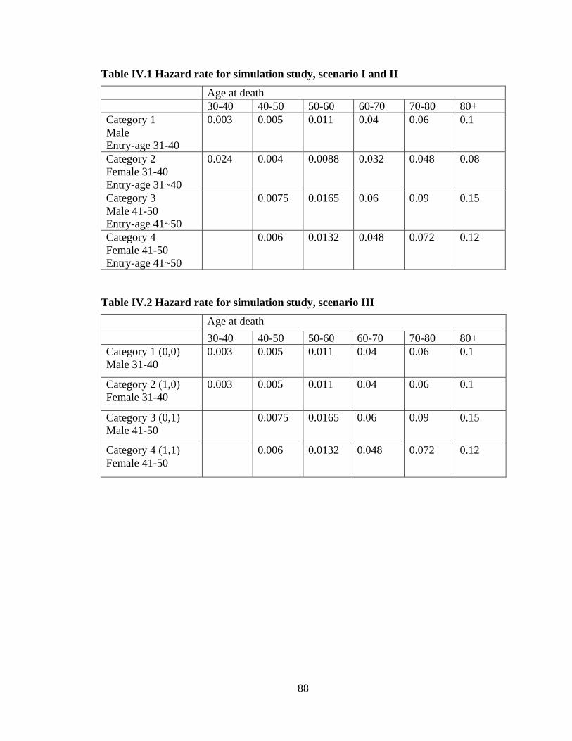
Table IV.1 Hazard rate for simulation study, scenario I and II
Age at death 30-40 40-50 50-60 60-70 70-80 80+ Category 1 Male Entry-age 31-40
0.003 0.005 0.011 0.04 0.06 0.1
Category 2 Female 31-40 Entry-age 31~40
0.024 0.004 0.0088 0.032 0.048 0.08
Category 3 Male 41-50 Entry-age 41~50
0.0075 0.0165 0.06 0.09 0.15
Category 4 Female 41-50 Entry-age 41~50
0.006 0.0132 0.048 0.072 0.12
Table IV.2 Hazard rate for simulation study, scenario III
Age at death 30-40 40-50 50-60 60-70 70-80 80+ Category 1 (0,0) Male 31-40
0.003 0.005 0.011 0.04 0.06 0.1
Category 2 (1,0) Female 31-40
0.003 0.005 0.011 0.04 0.06 0.1
Category 3 (0,1) Male 41-50
0.0075 0.0165 0.06 0.09 0.15
Category 4 (1,1) Female 41-50
0.006 0.0132 0.048 0.072 0.12
88

89
Table IV.3 Simulation study scenario I: inferences of regression coefficients from PH model
Entry-age (40~50) Gender (female) method Bias (*104)
RMSE** (*104)
Rel-wid
Cover
(%) Bias (*104)
RMSE (*104)
Rel-wid
Cover (%)
BD 38 570 1 95.2 -38 582 1 92.6 TC 11501 11513 0.94 0 486 746 0.99 84.8 HD1 8 574 1.01 94.6 183 623 1.01 93 HD2 25 571 1.01 95.4 257 622 1.01 91.8 HD3 7 569 1.01 95.2 276 645 1.01 91.2 HD4 36 573 1.01 94.8 -17 585 1 93.6 HD5 7 581 1.03 94.2 325 648 1.01 91
Table IV.4 Simulation study scenario II: inferences of regression coefficients from PH model
Entry-age (40~50) Gender (female) method Bias (*104)
RMSE (*104)
Rel-wid
Cover
(%) Bias (*104)
RMSE (*104)
Rel-wid
Cover
(%) BD 36 583 1 93.6 -15 580 1 93.6 TC 11463 11475 0.94 0 486 737 0.99 83.8 HD1 6 578 1.01 93.8 204 609 1.01 93.2 HD2 13 582 1.01 93.8 346 652 1.01 91.2 HD3 13 582 1.01 93.4 560 884 1.01 78.6 HD4 30 581 1.01 93.6 -7 577 1.01 94.2 HD5 96 599 1.03 93.6 225 588 1.02 94.2
** Here “RMSE” refers to root mean squared error. “Rel-wid” refers to “relative width”, which is fraction of 95 CI % width comparing to estimate 1. “Cover” refers to the 95% CI coverage.

90
Entry-age (40~50) Gender (female) Interaction method Bias (*104)
RMSE (*104)
Rel-width
Cover (%) Bias (*104)
RMSE (*104)
Rel-width
Cover (%) Bias (*104)
RMSE (*104)
Rel-width
Cover (%)
BD 28 781 1 94.2 -39 810 1 94.4 13 1094 1 95 TC 10383 10411 0.95 0 -710 1129 1.07 84.6 2423 2646 0.97 38.6 HD1 -217 836 1.01 92.8 -128 839 1.01 93 501 1277 1.01 90.2 HD2 -244 803 1.02 94.8 -53 803 1 93.8 568 1166 1.01 93.6 HD3 -241 823 1.01 94 -123 850 1.01 92.8 550 1298 1.01 89.4 HD4 -20 760 1.01 96.4 -67 798 1 94.6 104 1070 1.01 95.4 HD5 -706 985 1.04 88.8 -437 854 1.01 91 1452 1646 1.03 81.4
Table IV.5 Simulation study scenario III: inferences of regression coefficients from PH model

Table IV.6 Estimates of regression coefficients from PH model, original CHS data
Parameter Estimate (*10^4)
Standard Error (*10^4)
Pr > Chisq.
Hazard Raito
Entry-age 1 (40~44)
1977 1128 0.08 1.22
Entry-age 2 (45~49)
1814 1151 0.1 1.2
Entry-age 3 (50~59)
2786 1072 0.009 1.32
Entry-age 4 (60+)
2878 1242 0.02 1.33
Race/Gender 2 (white woman)
-4171 955 <0.0001 0.66
Race/Gender 3 (black man)
-241 949 0.8 0.98
Race/Gender 4 (black woman)
-1870 1031 0.07 0.83
Education 1 (some high school)
-1100 832 0.2 0.9
Education 2 (after high school)
-3761 1000 0.0002 0.69
Current cigarette smoking 1 (Yes)
5677 701 <0.0001 1.76
History of MI 1 (possible)
3741 3416 0.3 1.45
History of MI 2 (definite)
6949 1889 0.0002 2
History of diabetes 1 (Yes)
4330 1602 0.007 1.54
History of hypertension 1 (Yes)
1547 750 0.04 1.17
EKG 1 (with problem)
4644 947 <0.0001 1.59
Living place 20~65 2 (rural)
-2947 1028 0.004 0.75
Living place 20~65 3 ( mix of rural and urban )
-1361 1467 0.4 0.87
BMI 28 74 0.7 1
91

Table IV.7 Estimates of regression coefficients from PH model, CHS data after SDC
Estimate (SE) (*10^4)
BD TC HD1 HD2 HD3 HD4 HD5
Entry-age 1 (40~44)
1992 (1154)
2597 (1164)
2129 (1155)
1962 (1157)
1977 (1152)
1801 (1173)
Entry-age 2 (45~49)
1815 (1153)
1817 (1181)
2429 (1173)
1872 (1180)
1999 (1178)
2269 (1187)
Entry-age 3 (50~59)
2711 (1056)
1640 (1097)
2658 (1094)
2371 (1098)
2706 (1090)
2638 (1095)
Entry-age 4 (60+)
2799 (1254)
Entry- age 1 (<40) -792 (975)
2393 (1240)
3446 (1268)
2922 (1262)
3099 (1262)
3716 (1230)
Race/Gender 2 (white woman)
-4200 (913)
-3813 (1189)
-4724 (1002)
-2667 (953)
-3798 (979)
-3971 (965)
-2177 (960)
Race/Gender 3 (black man)
-205 (1004)
982 (1142)
-248 (966)
723 (960)
54 (975)
16 (963)
845 (971)
Race/Gender 4 (black woman)
-1876 (1073)
-1734 (1346)
-1984 (1036)
-1596 (1055)
-1771 (1054)
-1660 (1054)
-1267 (1043)
Education 1 (some high school)
-1127 (829)
-1347 (1029)
-996 (841)
-1108 (843)
-1224 (843)
-1257 (846)
-924 (847)
Education 2 (after high school)
-3806 (963)
-4958 (1257)
-3559 (1024)
-3081 (1003)
-3721 (1027)
-3793 (1013)
-3290 (1025)
Current cigarette smoking 1 (Yes)
5785 (718)
7328 (891)
5763 (714)
5463 (709)
5874 (724)
5596 (711)
4875 (706)
History of MI 1 (possible)
4211 (4548)
5360 (6113)
3397 (3515)
2702 (3483)
2467 (3516)
2946 (3599)
3863 (3552)
History of MI 2 (definite)
7080 (1936)
5622 (2766)
4678 (1980)
3392 (2027)
5029 (1979)
5280 (1954)
4716 (2017)
History of diabetes 1 (Yes)
4616 (2158)
6234 (2189)
4013 (1681)
3426 (1685)
3695 (1676)
4414 (1674)
4744 (1677)
History of hypertension 1 (Yes)
1637 (840)
2581 (977)
2006 (775)
1976 (769)
1877 (778)
1678 (777)
1823 (778)
EKG 1 (with problem)
4754 (1091)
4717 (1197)
4129 (982)
2421 (992)
3936 (982)
3754 (974)
3327 (992)
Living place 20~65 2 (rural)
-3042 (1029)
-3719 (1299)
-3297 (1054)
-2741 (1040)
-3189 (1058)
-3162 (1047)
-2522 (1039)
Living place 20~65 3 ( mix of rural and urban )
-1296 (1887)
-594 (1969)
-1375 (1545)
-397 (1474)
-1239 (1500)
-559 (1480)
-410 (1519)
BMI 28 (81)
20 (98)
57 (76)
40 (76)
61 (76)
13 (75)
10 (76)
92

Chapter V
Conclusion and Discussion
Statistical disclosure control is a field with increasing attention and interest nowadays.
Though progress has been made in implementing a variety of SDC techniques, these
methods are not totally satisfactory in providing sufficient protection while reducing
information loss. In this dissertation I propose both non-parametric and parametric MI
methods for disclosure limitation problems caused by extreme values of variable.
In Chapter II, I describe an approach to SDC of extreme values based on multiple
imputation of values beyond a cut-off. I illustrate the performance of these methods for
inference about the mean of a variable subject to SDC, by simulations and application to
data from the Chinese income project. We conclude that our hot-deck MI method, as well
as the MI methods with log-normal model fitted to the deleted data, and with power-
normal model fitted to the complete data, are decisively superior to top-coding in our
simulations. They all produce excellent inferences for the mean, with the method based
on power-normal model yielding imputations that match well the distribution of the
deleted values. The “D” method based on power-normal model also yields good
conference coverage but tends to be less efficient than the former methods; and the
93

method based on log-normal model fitted to the complete data is vulnerable to model
misspecification. I further introduce covariates into the analysis and assess impact of the
SDC methods on a regression where outcome is subject to top-coding. Our results prove
that when applying the MI method to multivariate data, we should condition the
predictive distribution of the deleted values on observed covariates, as failure to
condition on covariates leads to an attenuation of relationships between outcome and
covariates. I address this situation in Chapter III, by proposing stratified and regression-
based extensions of our MI methods.
The regression-based methods are potentially more efficient, but a bit more
complicated computationally than stratified methods. As for method performance, the
stratified and regression extensions of MI methods are in general superior to top-coding
and unconditional MI methods for inference about regression coefficient. Regression
method with log-normal model fitted to the deleted data has the best performance and
yield results close to before deletion. Stratified hot-deck method and the “D” method
based on log-normal model, and regression method with power-normal model fitted to
the complete data also produce good inferences. Regression method with power-normal
model fitted to the deleted data works well except when estimating the marginal mean of
outcome, with mis-specified model. Stratified MI methods based on power-normal model
work well when the outcome is subject to SDC. When the imputations are performed on a
covariate, they yield less satisfactory results. Both stratified and regression methods with
log-normal model fitted to the complete data vulnerable to misspecification.
94

Longitudinal data raise particular confidential concerns with potentially extensive
longitudinal information gathered over time, yet research on SDC method for
longitudinal study is very limited. In Chapter IV I consider a specific application
concerning disclosure risk caused by some participants attaining high ages because of
prolonged participation in a longitudinal study, and develop nonparametric, stratified MI
methods for this particular data setting.
I have focused on inference about regression coefficients from Cox’s proportional
hazard model. Among our stratified hot-deck MI methods, the method that retains the
censoring indicator (HD4) has the best performance and yields results close to before
deletion in simulation studies. The other stratified methods also work well overall, except
that sometimes they do not quite attain the nominal confidence coverage. The no-
stratification method works almost as well as stratified HD methods in simple data
settings. In situations with more covariates and a larger number of sensitive cases, it
yields biased estimates with low confidence coverage.
In this dissertation I present two different versions of parametric MI methods, the
“C” method which is based on a model fitted to the complete data; and the “D” method
based on a model fitted to the deleted values alone. The “C” method is efficient, but
vulnerable to model misspecification. The “D” method involves some loss of efficiency,
but is more robust to model misspecification, since the model is being fitted to the data
that are being deleted. This finding is further confirmed in Chapter IV, with two
alternative stratification methods. The first method calculates predicted values from
95

regression on the deleted data; and the second one utilizes the complete data for
regression. Results show the first method yields estimates with better inferential
properties, since regression on deleted data tends to be more robust to model mis-
specification.
Our MI methods have the following advantages over the standard approach, top-
coding. First, appropriate treatment of the top-coded data, using methods like maximum
likelihood for censored data, requires custom algorithms that are not widely available in
standard statistical software. In contrast, MI inferences only require complete-data
methods and simple MI combining rules. Second, the MI methods tend to be less
sensitive than top-coding to model mis-specification, as seen in our simulation studies.
For the data producer, MI has the advantage that the balance between disclosure
protection and information loss can be controlled by the choice of cut-off and number of
MI’s released. The use of MI allows imputation uncertainty to be propagated, and the
multiple imputations of a particular value enhance disclosure protection by making clear
to a potential snooper that these values are not real.
Overall, our proposed MI methods for SDC are relatively easy to implement, and
yield valid inferences close to those from the data before deletion in the situations
investigated. Thus, we expect these methods will prove valuable to practitioners.
On the other hand, the research in this dissertation is limited to a single variable
that needs disclosure protection and considered inference of the marginal mean of a
variable, or regression coefficient from a regression model. Future work should
96

investigate our SDC methods in multivariate analysis involving a set of variables that are
subject to disclosure limitation procedure.
Moreover, I have confined attention to the comparison of our methods with top-
coding. Other alternatives to top-coding, such as adding random noise to the values
beyond top-code are also of interest. More simulation studies that compare our MI
methods with these alternatives would be of interest.
Finally, my research of disclosure limitation methods for longitudinal data has
been limited to individuals with high age values. The whole field of SDC methods raised
by other variables (e.g. geographic) in longitudinal health data remains rather unexplored.
I also plan to consider other possible confidential concerns for longitudinal data and
develop suitable SDC methods for these problems.
97

Bibliography
98

Bibliography
Abowd, J.M. and Woodcock S.D. (2004). Multiply-imputing Confidential Characteristics and File Links in Longitudinal Linked Data. In “Privacy in Statistical Databases”. Domingo-Ferrer J. and Torra, V. (Eds.), Springer-Verlag, pp. 290-297.
An, D. and Little, R.J. (2007a). Multiple imputation: an alternative to top coding for statistical disclosure control. Journal of the Royal Statistical Society, Series A, 170, pp. 923-940.
An, D. and Little, R.J. (2007b). Extensions of multiple imputation methods as disclosure control procedure for multivariate data. In preparation.
Dalenius, T. and Reiss, S.P. (1982). Data-Swapping: A Technique for Disclosure Control. Journal of Statistical Planning and Inferences, 6, pp. 73-85.
Dempster, A.P., Laird, N. and Rubin, D.B. (1977). Maximum Likelihood from Incomplete Data via the EM Algorithm. Journal of the Royal Statistical Society, Series B, 39, pp. 1-37.
Fuller, W.A. (1993). Masking procedures for microdata disclosure limitation. Journal of Official Statistics, 2, pp. 383-406.
Kennickell, A.B. (1997). Multiple imputation and disclosure protection: The case of the 1995 Survey of Consumer Finances. Survey of Consumer Finances Working Papers.
Little, R.J.A. (1993). Statistical analysis of masked data. Journal of Official Statistics 9, pp. 407-426.
Little, R.J.A. and Rubin, DB (2002). Statistical Analysis with Missing Data. Wiley: New York.
Little, R.J., Liu, F. and Raghunathan, T. (2004). Statistical Disclosure Techniques Based on Multiple Imputation. In “Applied Bayesian Modeling and Causal Inference from Incomplete-Data Perspectives”, A. Gelman and X.-L. Meng, eds., pp. 141-152. Wiley: New York.
Nietert P.J., Sutherland S.E., Bachman D.L., Keil J.E., Gazes P., and Boyle E. (2000). CHARLESTON HEART STUDY [Computer file]. ICPSR version. Charleston, SC: Medical University of South Carolina [producer], 2000. Ann Arbor, MI: Inter-university Consortium for Political and Social Research [distributor], 2004.
R Project (2007). The R project for statistical computing. See http://www.r-project.org/.
99

Raghunathan, T.E., Reiter J.P., and Rubin, D.B. (2003). Multiple imputation for statistical disclosure limitation. Journal of Official Statistics, 19, pp. 1-16.
Reiter, J.P. (2002). Satisfying disclosure restrictions with synthetic data sets. Journal of Official Statistics, 18, pp. 531-544.
Reiter, J.P. (2003). Inference for partially synthetic, public use microdata sets. Survey Methodology, 29, pp. 181-188.
Reiter, J.P. (2005a). Releasing multiply-imputed, synthetic public use microdata: An illustration and empirical study. Journal of the Royal Statistical Society, Series A, 168, pp. 185 - 205.
Reiter, J.P. (2005b). Significance tests for multi-component estimands from multiply-imputed, synthetic microdata. Journal of Statistical Planning and Inference, 131 (2), pp. 365 - 377.
Riskin, C., Zhao R. and Li S. (2000). Chinese Household Income Project, 1995 [Computer file]. ICPSR version. Amherst, MA: University of Massachusetts, Political Economy Research Institute [producer]. Ann Arbor, MI: Inter-university Consortium for Political and Social Research [distributor]. http://webapp.icpsr.umich.edu/cocoon/ICPSR-STUDY/03012.xml
Rubin, D.B. (1993). Satisfying confidentiality constraints through use of synthetic multiply-imputed microdata. Journal of Official Statistics, 9, pp. 461-468.
U.S. Department of Commerce, U.S. Census Bureau. Survey of Income and Program Participation (2001).
U.S. Department of Health and Human Services. The Health Insurance Portability and Accountability Act (HIPAA) of 1996.
U.S. Department of Health and Human Services. Standards for Privacy of Individually Identifiable Health Information (the Privacy Rule).
100
Related Documents

![[MI] Multiple Imputation - Data Analysis and Statistical ... · Estimation using previously saved estimation results 68 ... imputation, which originated in early 1970 in application](https://static.cupdf.com/doc/110x72/5b05addf7f8b9a41528e029e/mi-multiple-imputation-data-analysis-and-statistical-using-previously-saved.jpg)


![[MI] Multiple Imputation - Duke Universitypublic.econ.duke.edu/stata/Stata-13-Documentation/mi.pdf · 2013-06-12 · Multiple imputation (MI) is a flexible, simulation-based statistical](https://static.cupdf.com/doc/110x72/5eb947f7f1f4b4048d5334ef/mi-multiple-imputation-duke-2013-06-12-multiple-imputation-mi-is-a-iexible.jpg)


