Multiple criteria aggregation procedure for mixed evaluations

European Journal of Operational Research 181 (2007) 1506–1515

www.elsevier.com/locate/ejor

Multiple criteria aggregation procedure for mixed evaluations

Sarah Ben Amor a,*, Khaled Jabeur b, Jean-Marc Martel a

a Departement des Operations et Systemes de Decision, F.S.A., Universite Laval, Que., Canada G1K 7P4b Recherche et Developpement pour la defense Canada – Valcartier, 2459 boulevard Pie-XI Nord, Val-Belair, Que., Canada G3J 1X5

Received 1 December 2004; accepted 1 November 2005Available online 12 May 2006

Abstract

Most of the existing multiple criteria decision-making methods handle one kind of the information imperfections at thesame time. Stochastic methods and fuzzy methods constitute typical examples of these methods. However, several multiplecriteria modelizations include simultaneously many kinds of the information imperfections. In this work, we propose amultiple criteria aggregation procedure which accepts mixed evaluations, i.e. evaluations which contain different naturesof imperfections. It is based on an adaptation of the stochastic dominance results.� 2006 Elsevier B.V. All rights reserved.

Keywords: Decision analysis; Multiple criteria analysis; Uncertainty modeling

1. Introduction

The majority of the existing discrete multiple cri-teria methods, which consider the informationimperfections, treat only one type of imperfectionat the time [1]. Let us note that most of theseprocedures are based on a probabilistic or a fuzzymodelization. However, many multiple criteriamodelizations imply often the presence of differentforms of imperfection at the same time. The multiplecriteria methods accepting mixed evaluations (punc-tual, stochastic, fuzzy or else) are rather rare. Wefind in the literature at least two: NAIADE [17]and PAMSSEM [14,6].

0377-2217/$ - see front matter � 2006 Elsevier B.V. All rights reserved

doi:10.1016/j.ejor.2005.11.048

* Corresponding author.E-mail addresses: [email protected] (S.B. Amor),

[email protected] (K. Jabeur), [email protected] (J.-M. Martel).

Multiple criteria methods are based on the(A,X,E) model, where A is a set of potential alterna-tives, X is a finite set of attributes (or criteria) and E

is a performances table or an evaluation matrix.Some methods associate to each attribute/criterionj a coefficient of relative importance (or weight) wj,where

Pnj¼1wj ¼ 1. We have

.

Operational Research 181 (2007) 1506–1515 1507

It should be observed that the information imper-

Table 1Performance matrix for the attribute j

Alternatives Xj

xj1 � � � xj

h � � � xjH

a1... ..

.

ai . . . xhij . . .

..

. ...

am

Table 2Performance matrix for the attribute j integrating the a prioriinformation

Alternatives Any focal elements

Bj1 . . . Bj

h0 . . . Bj2H

a1 C11j . . . Ch0

1j . . . C2H

1j... ..

. ... ..

.

ai C1ij . . . Ch0

ij . . . C2H

ij... ..

. ... ..

.

am C1mj . . . Ch0

mj . . . C2H

mjA priori belief masses mðBj

1Þ . . . mðBjh0 Þ . . . mðBj

2H Þ

fection would notably appear in the evaluations eij.The aim of the NAIADE and PAMSSEM meth-

ods is to establish binary relations between the dif-ferent pairs of alternatives according to eachcriterion. These relations are then aggregated toproduce ‘‘global’’ relations between the pairs ofalternatives, which are exploited afterwards.

Since the evaluations are mixed (different naturesof the imperfections), the aggregation of the valuedlocal relations for all the pairs of alternatives issometimes difficult. In fact, the signification of thenumerical values at the local level could be unclearbecause of the heterogeneity of the measurementscales and the natures of the evaluations. Conse-quently, conciliating the results of the pair compar-isons according to the criteria could be difficult.This observation led us to use all available infor-mation to establish ‘‘crisp’’ relations locally betweenall the pairs of alternatives, then, to aggregatethem.

In the beginning of this paper, a general model-ing framework will be presented to clarify the con-text in which the proposed procedure is applied(Section 2). Our multiple criteria procedure formixed evaluations comprises two main phases. Thefirst phase (Section 3) consists of constructing thelocal preference relations. This construction is basedon an extension of the stochastic dominance con-cept to the mixed evaluations context; the stochasticdominance providing a uniform treatment in thiscontext. The second phase (Section 4) consists ofaggregating these local binary relations into globalbinary relations using an algorithm developed in agroup decision context and adapted to the multicri-teria aggregation [7]. The global preference relationsare then exploited (Section 5) using original proce-dures [7]. Finally, in Section 6, we conclude and dis-cuss future work.

2. General modeling framework

The adopted framework accepts, in the uncertaindecision-making situations, stochastic, possibilisticor ‘‘evidential’’ evaluations. It also includes fuzzyor ordinal evaluations. We think that among allincertitude-modeling languages (evidence theory,possibility theory and probability theory), the evi-dence theory presents the more general frameworkwhere possibilities and probabilities are proposedas particular cases. We exploit this property to settleour modelization.

S.B. Amor et al. / European Journal of

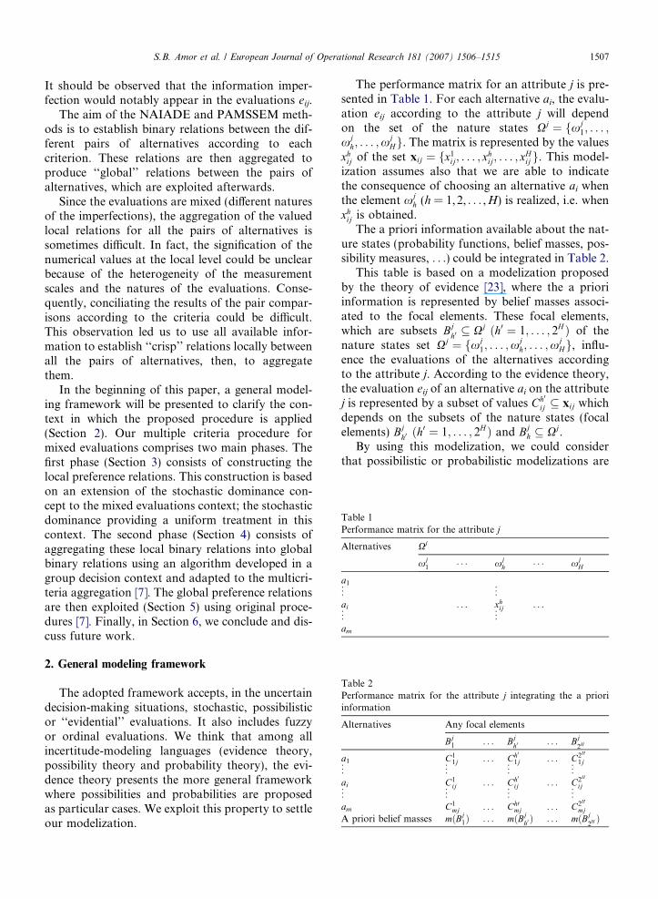
The performance matrix for an attribute j is pre-sented in Table 1. For each alternative ai, the evalu-ation eij according to the attribute j will dependon the set of the nature states Xj ¼ fxj

1; . . . ;xj

h; . . . ;xjHg. The matrix is represented by the values

xhij of the set xij ¼ fx1

ij; . . . ; xhij; . . . ; xH

ij g. This model-ization assumes also that we are able to indicatethe consequence of choosing an alternative ai whenthe element xj

h (h = 1,2, . . . ,H) is realized, i.e. whenxh

ij is obtained.The a priori information available about the nat-

ure states (probability functions, belief masses, pos-sibility measures, . . .) could be integrated in Table 2.

This table is based on a modelization proposedby the theory of evidence [23], where the a prioriinformation is represented by belief masses associ-ated to the focal elements. These focal elements,which are subsets Bj

h0 � Xj ðh0 ¼ 1; . . . ; 2H Þ of thenature states set Xj ¼ fxj

1; . . . ;xjh; . . . ;xj

Hg, influ-ence the evaluations of the alternatives accordingto the attribute j. According to the evidence theory,the evaluation eij of an alternative ai on the attributej is represented by a subset of values Ch0

ij � xij whichdepends on the subsets of the nature states (focalelements) Bj

h0 ðh0 ¼ 1; . . . ; 2H Þ and Bj

h � Xj.By using this modelization, we could consider

that possibilistic or probabilistic modelizations are

1508 S.B. Amor et al. / European Journal of Operational Research 181 (2007) 1506–1515

particular cases when the a priori information isrepresented by possibility or probability distribu-tions respectively. In fact, when the attribute is apossibilistic one, the a priori information relatedto the evaluation eij is characterized by possibilitydistributions p. In such a context, the correspondingbelief masses are associated with focal elements thatare embedded Bj

1 � � � � � Bjh0 � � � � � Bj

H 0 . The possi-bility measures coincide with the plausibilities of theembedded focal elements. When the attribute j isstochastic, the focal elements Bj

h0 are reduced tothe singletons {xj

h} and the corresponding beliefmasses correspond to probability measures. In thiscase, the evaluations are characterized by randomvariables X h

ij with a priori probability distributionsf h

ij . We have then the a priori (subjective) probabil-ities P h

j for each state of the nature xjh ðh ¼ 1;

2; . . . ;HÞ.

3. Local preference relations

The first phase of our procedure consists ofestablishing the local preference relations betweentwo alternatives. Let Hj be the local relationbetween two alternatives ai and ak on a criterion j.We have: ai Hj ak, where Hj = {�,��1,�, ?} with� is the indifference relation, � is the strict prefer-ence relation, ��1 is the inverse strict preferencerelation and ? is the incomparability relation.

In order to construct these relations, we privilegethe approach based on the extension of the stochas-tic dominance concept. The use of the stochasticdominance concept has the advantage of providinga uniform treatment for the different languageswhich express the information imperfections.Notice that stochastic dominance allows to con-clude about the preference of an alternative ai overan alternative ak for a decision-maker whose atti-tude towards risk corresponds to DARA (Decreas-ing Absolute Risk Aversion) utility functions [15].This type of risk aversion is observed for severaleconomic phenomena. The link between stochasticdominance and the preference is well known forthis class of utility functions. It is not always easyto make the decision-maker’s preferences explicitand we can often conclude that ai is preferred toak if some stochastic dominance conditions areverified.

In the case where the evaluation eij is a randomvariable, the results of stochastic dominance couldbe directly applied in order to establish preferencerelations. For instance, we could say that

eij �j ekj () jH 1ðxÞj ¼ jF ijðxÞ � F kjðxÞj 6 sj;

8x 2 ½xj�; x�j �;

where xj� and x�j are, respectively, the inferior andsuperior limits of the evaluation scale of attribute/criterion j, sj P 0 is a predetermined threshold, Fij

and Fkj are the cumulated probability distributionsfor the evaluations of alternatives ai and ak throughan attribute j and x is a modality of this attribute.

Otherwise, i.e. for the cases where jH1(x)j > sj

(Fij 5 Fkj), we can say that

eij �j ekj () eij FSDj or SSDj or TSDjekj;

eij ?j ekj () eij non SDj ekj;

where SD* means that one of the three dominancetypes is verified. The definitions of the dominancefor first order, second order and third order (FSD,SSD and TSD) can be found in [15] and AppendixA.

These concepts can be extended to ambiguousprobabilities [13]. For fuzzy, possibilistic or eviden-tial criteria, we propose the use of some transforma-tions which provide to the functions characterizingthe evaluation of an alternative on a given criterion(fuzzy membership functions, possibility distribu-tions, belief masses, . . .) properties similar to thoseof a probability density function.

For evidential criteria we use the pignistic trans-formation justified by Smets [24,25]

BetPðxhÞ ¼X

Bjb0 :x

jh2Bj

h0 �PðXÞ

mðBjh0 Þ

jBjh0 jð1� mð;ÞÞ

;

8Bjh0 2 PðXÞ; mð;Þ 6¼ 1;

where jBjh0 j is the cardinality of X in Bj

h0 andBetP(xh) is the pignistic probability of xh.

For possibilistic criteria we use the relation pro-posed by Dubois et al. [5]. This relation is equivalentto the pignistic transformation when applied to pos-sibility measures. The probability ph correspondingto xh is given by

ph ¼XH

t¼h

1

t� mt ¼

XH

t¼h

1

tðPt �Ptþ1Þ;

where mh is the belief mass m(Bh) (h = 1,2, . . . ,H),Bh are embedded and organized in sequence, i.e.B1 = {x1}, B2 = {x1,x2}, . . . , Bh = {x1,x2, . . . ,xh}, . . . , BH = X such that "B 5 Bh, m(B) = 0and it is possible for a certain h that m(Bh) = 0,

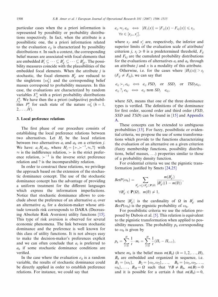
Table 3Numerical values associated to the D measure of distance

ai � ak ai � ak ai ? ak ai ��1 ak

ai � ak 0 4/3 1 4/3ai � ak 4/3 0 1 5/3ai ? ak 1 1 0 1ai ��1 ak 4/3 5/3 1 0

S.B. Amor et al. / European Journal of Operational Research 181 (2007) 1506–1515 1509

Ph = P({xh}) and P is the possibility measure de-fined for {xh}: PðfxhgÞ ¼ p‘ðfxhgÞ ¼

PHt¼hmt.

For fuzzy criteria we use the rescaling approachas proposed in Munda [17]

fijðxijÞ ¼ kijlijðeijÞ where

Z 1

�1fijðxijÞdxij ¼ 1:

Let us note that the construction of local preferencerelations for deterministic criteria can be carried outby using discrimination thresholds to distinguish be-tween strict preference and indifference situations(quasi-criterion notion) in the context of punctualevaluations. In this case, locally there is no incom-parability. It is one of the characteristics of a crite-rion [20].

4. Aggregating local preference relations

Once the local preference relations are estab-lished, the second stage of our procedure aims ataggregating n binary relations Hj (ai Hj ak) in orderto obtain a global binary relation H (ai H ak) byconsidering the relative importance of the criteria.

To achieve this, the algorithm (AL3) developedby Jabeur and Martel [8] in a group decision-mak-ing context was adapted. AL3 starts by defining,for each pair of alternatives (ai,ak), an indexUH(ai,ak) where H 2 {�,��1,�, ?}. This index mea-sures the divergence between the global relation H

and the local binary relations relating this pair ofalternatives on each criterion. This divergence willbe quantified by using the distance measure Dbetween binary relations relating two pairs of alter-natives [12].

The index UH(ai,ak) is determined as follows:

UHðai; akÞ ¼Xn

j¼1

wjDðH ;Rjðai; akÞÞ;

where

Rjðai; akÞ ¼

� if ai �j ak;

� if ai �j ak;

? if ai ?j ak;

��1 if ak �j ai:

8>>><>>>:

wj is the normalized coefficient of the relative impor-tance of criterion j, Rj(ai,ak) represents the local bin-ary relation comparing ai to ak on criterion j, D is adistance measure between the binary relations relat-ing the pairs of alternatives and H 2 {�,��1,�, ?}is the global relation. In the literature, some meth-ods are proposed to establish the relative impor-

tance of the criteria wj. Regarding this issue, onecan refer to Mousseau [16] and Roy and Mousseau[21].

In order to build the D distance measure, Jabeuret al. [12] proposed first a set of five ‘‘logic’’ condi-tions (an axiomatic) in which they compared the dis-tance between each pair of binary relations{�,��1,�, ?}. Then, they prove that D is a metric,i.e. it verifies the non-negativity, the symmetry andthe triangular inequality axioms. Finally, Jabeuret al. [12] chose the centroid of the variation domainof these pairwise comparisons to associate numeri-cal values to D (see Table 3). According to theseauthors, their distance measure brings someimprovements to the distance measures proposedby Roy and Slowinski [22] and Ben Khelifa andMartel [2].

Once the divergence indexes have been com-puted, we identify, for each pair of alternatives(ai,ak), the set of the global relations H* that mini-mize the indexes of divergence UH(ai,ak), that is

H� ¼ H �=UH� ¼ minH2f�;��1;�;?g

UHðai; akÞ� �

:

Therefore, if the set H* is reduced to a singleton, i.e.there is only one global relation H* that minimizesthe indexes of divergence UH(ai,ak), then H* willbe retained for the pair of alternatives (ai,ak) glob-ally. In the opposite case, i.e. where 2, 3 or 4 distinctrelations minimize the indexes of divergenceUH(ai,ak), priority rules have to be applied betweenthe binary relations {�,��1,�, ?}. We adopt thetwo priority rules proposed by Jabeur [7]. The firstone points out that the preference relation priorityis higher than that of the indifference relation andthe second rule indicates that the indifference rela-tion priority is higher than that of the incomparabil-ity relation.

Once the priority rules are applied, we analyzethe cardinality of H*. If H* contains a unique rela-tion H*, then H* will be retained for the pair ofalternatives (ai,ak) globally. In the opposite case,i.e. when H* contains two relations of the same

Table 4Performance matrices for X1, X2, X3 and X4

ai X1 X2 X3 X4 Associated fuzzy numbers

x11 x1

2 x13 x1

4 x15 x2

1 x22 x2

3 x31 x3

2 x33

a1 3 1 2 6 4 90 90 110 35 70 45 Weak (0, .1,0, .2)a2 1 3 4 6 3 120 90 100 45 30 45 Fair (.5, .5, .2, .2)a3 2 1 2 3 5 110 130 80 45 60 25 High (.9,1, .2,0)a4 6 1 4 4 2 80 110 120 40 70 30 More or less weak (.2, .2, .2, .2)

Fig. 1. Membership function for fuzzy trapezoidal number(a,b,c,d).

Table 5A priori information for X1

x11 x1

2 x13 x1

4 x15

P ðx1hÞ 0.28 0.23 0.10 0.28 0.11

1510 S.B. Amor et al. / European Journal of Operational Research 181 (2007) 1506–1515

priority (necessarily the preference (�) and theinverse preference (��1) relations), we apply theintersection rule used by Roy [19] to combine twocomplete orders, and therefore, the incomparabilityrelation (H* ?) will be retained for the pair ofalternatives (ai,ak) globally.

The algorithm AL3 could be summarized asfollows:

Step 1: Let B = {(ai,ak)/(ai,ak) 2 A · A} the set ofthe alternatives pairs. Compute for all alter-natives pairs of B and for eachH 2 {�,��1,�, ?} the divergence indexUH(ai,ak).

Step 2: Identify for each alternatives pair of B theset of global relations H*. If H* contains aunique relation, then this relation wouldbe retained for the alternatives pair (ai,ak)globally. If not, go to step 3.

Step 3: Apply the priority rules. If H* contains aunique relation, then this relation wouldbe retained for the pair of alternatives(ai,ak) globally. If not, go to step 4.

Step 4: Apply the intersection rule to retain theincomparability relation for the alternativespair (ai,ak) globally.

Notice that this algorithm requires n(n � 1)/2iterations to establish a global preference relationalsystem (p.r.s) from local preference relational sys-tems. Moreover, this algorithm guarantees the inde-pendence towards the irrelevant alternatives. Then,adding or removing an irrelevant alternative at willnot modify in any case the type of the relationbetween ai and ak globally. Once the global p.r.s isdetermined, it could be exploited according to differ-ent decisional problematics (e.g., the choice prob-lematic, the ranking problematic, or the sortingproblematic). In the literature, several exploitationprocedures can be found. One can quote the worksof Roy [18], Colson [4] and Jabeur and Martel [9]for the choice problematic; the works of Roy [19],Brans and Vincke [3], Colson [4] and Jabeur and

Martel [10] for the ranking problematic; and theworks of Yu [26] and Jabeur and Martel [11] forthe sorting problematic.

4.1. Numerical example

Let us consider the following illustrative examplefor the proposed multiple criteria aggregation pro-cedure: A = {a1,a2,a3,a4} and X = {X1,X2,X3,X4}where X1 is a stochastic attribute, X2 is an evidentialattribute, X3 is a possibilistic attribute and X4 is afuzzy attribute. For each attribute, the inputs con-sist of the performance matrix, the a priori informa-tion, and the indifference threshold.

Table 4 gives the performance matrices for thefour attributes. The evaluations according to X4

are linguistic variables represented by trapezoidalfuzzy numbers (a,b,c,d) (see Fig. 1).

Table 5 gives the a priori information for attri-bute X1, while Table 6 gives the a priori informationfor X2 and X3. For attribute X4, the a priori infor-mation is implicitly contained in the performancematrix. We consider the same indifference thresholdfor all the attributes, i.e. s1 = s2 = s3 = s4 = s =0.05.

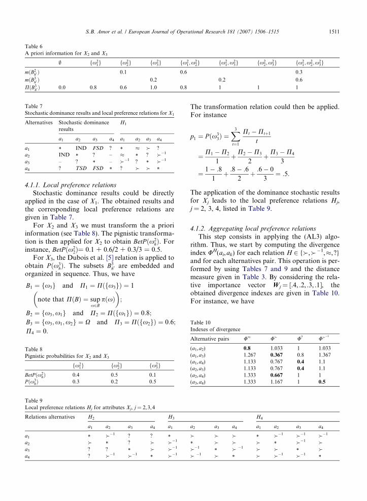
Table 7Stochastic dominance results and local preference relations for X1

Alternatives Stochastic dominanceresults

H1

a1 a2 a3 a4 a1 a2 a3 a4

a1 * IND FSD ? * � � ?a2 IND * ? – � * ? ��1

a3 – ? * – ��1 ? * ��1

a4 ? TSD FSD * ? � � *

Table 10Indexes of divergence

Alternative pairs U� U� U? U��1

Table 6A priori information for X2 and X3

; fx21g fx2

2g fx23g fx2

1;x22g fx2

1;x23g fx2

2;x23g fx2

1;x22;x

23g

mðB2h0 Þ 0.1 0.6 0.3

mðB3h0 Þ 0.2 0.2 0.6

PðB3h0 Þ 0.0 0.8 0.6 1.0 0.8 1 1 1

S.B. Amor et al. / European Journal of Operational Research 181 (2007) 1506–1515 1511

4.1.1. Local preference relations

Stochastic dominance results could be directlyapplied in the case of X1. The obtained results andthe corresponding local preference relations aregiven in Table 7.

For X2 and X3 we must transform the a prioriinformation (see Table 8). The pignistic transforma-tion is then applied for X2 to obtain BetP ðx2

hÞ. Forinstance, BetP ðx2

2Þ= 0.1 + 0.6/2 + 0.3/3 = 0.5.For X3, the Dubois et al. [5] relation is applied to

obtain P ðx3hÞ. The subsets B3

h0 are embedded andorganized in sequence. Thus, we have

B1 ¼ fx3g and P1 ¼ Pðfx3gÞ ¼ 1

note that PðBÞ ¼ supx2B

pðxÞ� �

;

B2 ¼ fx3;x1g and P2 ¼ Pðfx1gÞ ¼ 0:8;

B3 ¼ fx3;x1;x2g ¼ X and P3 ¼ Pðfx2gÞ ¼ 0:6;

P4 ¼ 0:

Table 8Pignistic probabilities for X2 and X3

fx21g fx2

2g fx23g

BetPðx2hÞ 0.4 0.5 0.1

P ðx3hÞ 0.3 0.2 0.5

Table 9Local preference relations Hj for attributes Xj, j = 2,3,4

Relations alternatives H2 H3

a1 a2 a3 a4 a1

a1 * ��1 ? ? *a2 � * ? � ��1

a3 ? ? * � ��1

a4 ? ��1 ��1* ��1

The transformation relation could then be applied.For instance

p1 ¼ P ðx33Þ ¼

X3

t¼1

Pt �Ptþ1

t

¼ P1 �P2

1þP2 �P3

2þP3 �P4

3

¼ 1� :81þ :8� :6

2þ :6� 0

3¼ :5:

The application of the dominance stochastic resultsfor Xj leads to the local preference relations Hj,j = 2, 3, 4, listed in Table 9.

4.1.2. Aggregating local preference relations

This step consists in applying the (AL3) algo-rithm. Thus, we start by computing the divergenceindex UH(ai,ak) for each relation H 2 {�,��1,�, ?}and for each alternatives pair. This operation is per-formed by using Tables 7 and 9 and the distancemeasure given in Table 3. By considering the rela-tive importance vector Wj = [.4, .2, .3, .1], theobtained divergence indexes are given in Table 10.For instance, we have

H4

a2 a3 a4 a1 a2 a3 a4

� � � * ��1 ��1 ��1

* � � � * ��1 ���1

* � �1 � � * �� �1 � * � ��1 ��1

*

(a1,a2) 0.8 1.033 1 1.033(a1,a3) 1.267 0.367 0.8 1.367(a1,a4) 1.133 0.767 0.4 1.1(a2,a3) 1.133 0.767 0.4 1.1(a2,a4) 1.333 0.667 1 1(a3,a4) 1.333 1.167 1 0.5

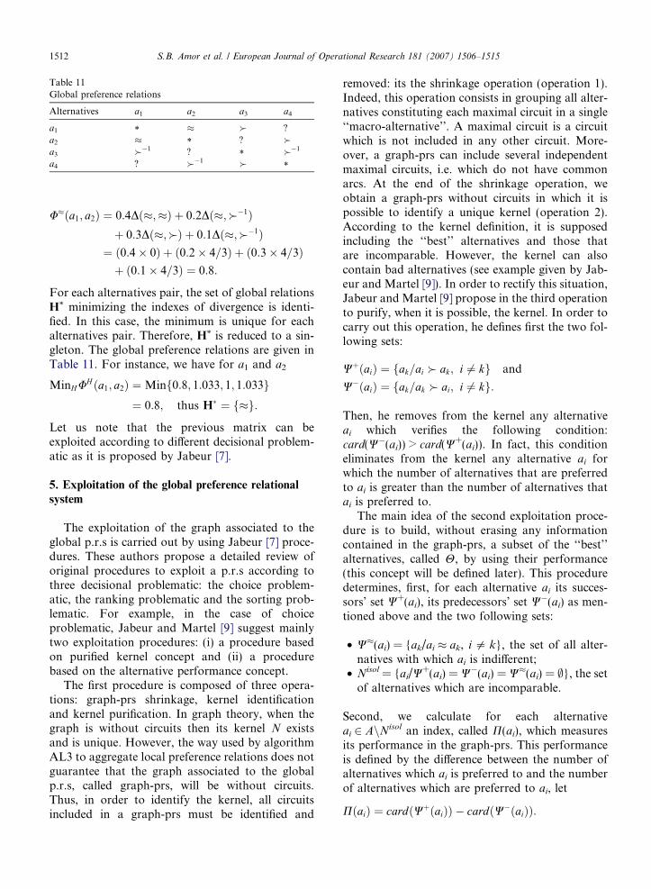
Table 11Global preference relations

Alternatives a1 a2 a3 a4

a1 * � � ?a2 � * ? �a3 ��1 ? * ��1

a4 ? ��1 � *

1512 S.B. Amor et al. / European Journal of Operational Research 181 (2007) 1506–1515

U�ða1; a2Þ ¼ 0:4Dð�;�Þ þ 0:2Dð�;��1Þþ 0:3Dð�;�Þ þ 0:1Dð�;��1Þ¼ ð0:4 0Þ þ ð0:2 4=3Þ þ ð0:3 4=3Þþ ð0:1 4=3Þ ¼ 0:8:

For each alternatives pair, the set of global relationsH* minimizing the indexes of divergence is identi-fied. In this case, the minimum is unique for eachalternatives pair. Therefore, H* is reduced to a sin-gleton. The global preference relations are given inTable 11. For instance, we have for a1 and a2

MinHUH ða1; a2Þ ¼Minf0:8; 1:033; 1; 1:033g¼ 0:8; thus H� ¼ f�g:

Let us note that the previous matrix can beexploited according to different decisional problem-atic as it is proposed by Jabeur [7].

5. Exploitation of the global preference relationalsystem

The exploitation of the graph associated to theglobal p.r.s is carried out by using Jabeur [7] proce-dures. These authors propose a detailed review oforiginal procedures to exploit a p.r.s according tothree decisional problematic: the choice problem-atic, the ranking problematic and the sorting prob-lematic. For example, in the case of choiceproblematic, Jabeur and Martel [9] suggest mainlytwo exploitation procedures: (i) a procedure basedon purified kernel concept and (ii) a procedurebased on the alternative performance concept.

The first procedure is composed of three opera-tions: graph-prs shrinkage, kernel identificationand kernel purification. In graph theory, when thegraph is without circuits then its kernel N existsand is unique. However, the way used by algorithmAL3 to aggregate local preference relations does notguarantee that the graph associated to the globalp.r.s, called graph-prs, will be without circuits.Thus, in order to identify the kernel, all circuitsincluded in a graph-prs must be identified and

removed: its the shrinkage operation (operation 1).Indeed, this operation consists in grouping all alter-natives constituting each maximal circuit in a single‘‘macro-alternative’’. A maximal circuit is a circuitwhich is not included in any other circuit. More-over, a graph-prs can include several independentmaximal circuits, i.e. which do not have commonarcs. At the end of the shrinkage operation, weobtain a graph-prs without circuits in which it ispossible to identify a unique kernel (operation 2).According to the kernel definition, it is supposedincluding the ‘‘best’’ alternatives and those thatare incomparable. However, the kernel can alsocontain bad alternatives (see example given by Jab-eur and Martel [9]). In order to rectify this situation,Jabeur and Martel [9] propose in the third operationto purify, when it is possible, the kernel. In order tocarry out this operation, he defines first the two fol-lowing sets:

WþðaiÞ ¼ fak=ai � ak; i 6¼ kg and

W�ðaiÞ ¼ fak=ak � ai; i 6¼ kg:

Then, he removes from the kernel any alternativeai which verifies the following condition:card(W�(ai)) > card(W+(ai)). In fact, this conditioneliminates from the kernel any alternative ai forwhich the number of alternatives that are preferredto ai is greater than the number of alternatives thatai is preferred to.

The main idea of the second exploitation proce-dure is to build, without erasing any informationcontained in the graph-prs, a subset of the ‘‘best’’alternatives, called H, by using their performance(this concept will be defined later). This proceduredetermines, first, for each alternative ai its succes-sors’ set W+(ai), its predecessors’ set W�(ai) as men-tioned above and the two following sets:

• W�(ai) = {ak/ai � ak, i 5 k}, the set of all alter-natives with which ai is indifferent;

• Nisol = {ai/W+(ai) = W�(ai) = W�(ai) = ;}, the set

of alternatives which are incomparable.

Second, we calculate for each alternativeai 2 AnNisol an index, called P(ai), which measuresits performance in the graph-prs. This performanceis defined by the difference between the number ofalternatives which ai is preferred to and the numberof alternatives which are preferred to ai, let

PðaiÞ ¼ cardðWþðaiÞÞ � cardðW�ðaiÞÞ:

4a

1a

3a

2a

Indifference Preference Incomparability

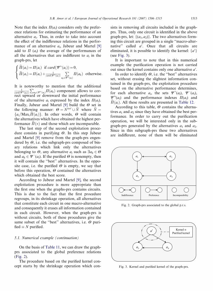
Fig. 2. Graph-prs associated to the global p.r.s.

S.B. Amor et al. / European Journal of Operational Research 181 (2007) 1506–1515 1513

Note that the index P(ai) considers only the prefer-ence relations for estimating the performance of analternative ai. Thus, in order to take into accountthe effect of the indifference relations in the perfor-mance of an alternative ai, Jabeur and Martel [9]add to P (ai) the average of the performances ofall the alternatives that are indifferent to ai in thegraph-prs, let

bPðaiÞ¼PðaiÞ if cardðW�ðaiÞÞ¼ 0;bPðaiÞ¼PðaiÞþ 1cardðW�ðaiÞÞ

Pak2W�ðaiÞ

PðakÞ otherwise:

8<:It is noteworthy to mention that the additional

1cardðW�ðaiÞÞ

Pak2W�ðaiÞPðakÞ component allows to cor-

rect upward or downward the initial performanceof the alternative ai expressed by the index P(ai).Finally, Jabeur and Martel [9] build the H set inthe following manner: H ¼ Nisol [ bN where bN ¼fai=Maxi

bPðaiÞg. In other words, H will containthe alternatives which have obtained the highest per-formance bPð�Þ and those which are incomparable.

The last step of the second exploitation proce-dure consists in purifying H. In this step Jabeurand Martel [9] remove from the graph-prs engen-dered by H, i.e. the subgraph-prs composed of bin-ary relations which link only the alternativesbelonging to H, any alternative ai such as $ak 2 Hand ak 2 W�(ai). If the purified H is nonempty, thenit will contain the ‘‘best’’ alternatives. In the oppo-site case, i.e. the purified H is empty, we say thatbefore this operation, H contained the alternativeswhich obtained the best score.

According to Jabeur and Martel [9], the secondexploitation procedure is more appropriate thanthe first one when the graphs-prs contains circuits.This is due to the fact that the first procedureregroups, in its shrinkage operation, all alternativesthat constitute each circuit in one macro-alternativeand consequently it erases all information containedin each circuit. However, when the graph-prs iswithout circuits, both of these procedures give thesame subset of the ‘‘best’’ alternatives, i.e. H puri-fied N purified.

Kernel ≡Purified kernel

'a

3a 4a

Fig. 3. Kernel and purified kernel of the graph-prs.

5.1. Numerical example (continuation)

On the basis of Table 11, we can draw the graph-prs associated to the global preference relations(Fig. 2).

The procedure based on the purified kernel con-cept starts by the shrinkage operation which con-

sists in removing all circuits included in the graph-prs. Thus, only one circuit is identified in the abovegraph-prs, let: {(a1,a2)}. The two alternatives form-ing this circuit are grouped in a single ‘‘macro-alter-native’’ called a 0. Once that all circuits areeliminated, it is possible to identify the kernel: {a 0}(see Fig. 3).

It is important to note that in this numericalexample the purification operation is not carriedout since the kernel contains only one alternative a 0.

In order to identify H, i.e. the ‘‘best’’ alternativesset, without erasing the slightest information con-tained in the graph-prs, the exploitation procedurebased on the alternative performance determines,for each alternative ai, the sets W+(ai), W�(ai),W�(ai) and the performance indexes P(ai) andbPðaiÞ. All these results are presented in Table 12.

According to this table, H contains the alterna-tives a1 and a2 since they have obtained the best per-formance. In order to carry out the purificationoperation, we will be interested only in the sub-graph-prs generated by the alternatives a1 and a2.Since in this subgraph-prs these two alternativesare indifferent, none of them will be eliminated

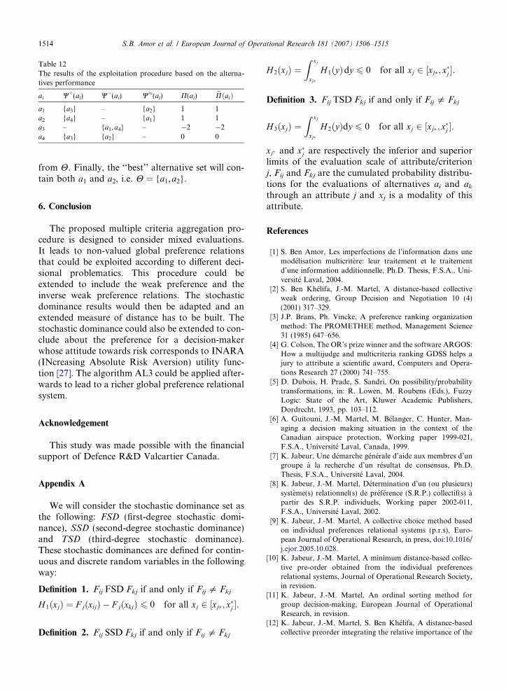
Table 12The results of the exploitation procedure based on the alterna-tives performance

ai W+(ai) W�(ai) W�(ai) P(ai) bPðaiÞa1 {a3} – {a2} 1 1a2 {a4} – {a1} 1 1a3 – {a1,a4} – �2 �2a4 {a3} {a2} – 0 0

1514 S.B. Amor et al. / European Journal of Operational Research 181 (2007) 1506–1515

from H. Finally, the ‘‘best’’ alternative set will con-tain both a1 and a2, i.e. H = {a1,a2}.

6. Conclusion

The proposed multiple criteria aggregation pro-cedure is designed to consider mixed evaluations.It leads to non-valued global preference relationsthat could be exploited according to different deci-sional problematics. This procedure could beextended to include the weak preference and theinverse weak preference relations. The stochasticdominance results would then be adapted and anextended measure of distance has to be built. Thestochastic dominance could also be extended to con-clude about the preference for a decision-makerwhose attitude towards risk corresponds to INARA(INcreasing Absolute Risk Aversion) utility func-tion [27]. The algorithm AL3 could be applied after-wards to lead to a richer global preference relationalsystem.

Acknowledgement

This study was made possible with the financialsupport of Defence R&D Valcartier Canada.

Appendix A

We will consider the stochastic dominance set asthe following: FSD (first-degree stochastic domi-nance), SSD (second-degree stochastic dominance)and TSD (third-degree stochastic dominance).These stochastic dominances are defined for contin-uous and discrete random variables in the followingway:

Definition 1. Fij FSD Fkj if and only if Fij 5 Fkj

H 1ðxjÞ ¼ F jðxijÞ � F jðxkjÞ 6 0 for all xj 2 ½xj�; x�j �:

Definition 2. Fij SSD Fkj if and only if Fij 5 Fkj

H 2ðxjÞ ¼Z xj

xj�

H 1ðyÞdy 6 0 for all xj 2 ½xj�; x�j �:

Definition 3. Fij TSD Fkj if and only if Fij 5 Fkj

H 3ðxjÞ ¼Z xj

xj�

H 2ðyÞdy 6 0 for all xj 2 ½xj�; x�j �:

xj� and x�j are respectively the inferior and superiorlimits of the evaluation scale of attribute/criterionj, Fij and Fkj are the cumulated probability distribu-tions for the evaluations of alternatives ai and ak

through an attribute j and xj is a modality of thisattribute.

References

[1] S. Ben Amor, Les imperfections de l’information dans unemodelisation multicritere: leur traitement et le traitementd’une information additionnelle, Ph.D. Thesis, F.S.A., Uni-versite Laval, 2004.

[2] S. Ben Khelifa, J.-M. Martel, A distance-based collectiveweak ordering, Group Decision and Negotiation 10 (4)(2001) 317–329.

[3] J.P. Brans, Ph. Vincke, A preference ranking organizationmethod: The PROMETHEE method, Management Science31 (1985) 647–656.

[4] G. Colson, The OR’s prize winner and the software ARGOS:How a multijudge and multicriteria ranking GDSS helps ajury to attribute a scientific award, Computers and Opera-tions Research 27 (2000) 741–755.

[5] D. Dubois, H. Prade, S. Sandri, On possibility/probabilitytransformations, in: R. Lowen, M. Roubens (Eds.), FuzzyLogic: State of the Art, Kluwer Academic Publishers,Dordrecht, 1993, pp. 103–112.

[6] A. Guitouni, J.-M. Martel, M. Belanger, C. Hunter, Man-aging a decision making situation in the context of theCanadian airspace protection, Working paper 1999-021,F.S.A., Universite Laval, Canada, 1999.

[7] K. Jabeur, Une demarche generale d’aide aux membres d’ungroupe a la recherche d’un resultat de consensus, Ph.D.Thesis, F.S.A., Universite Laval, 2004.

[8] K. Jabeur, J.-M. Martel, Determination d’un (ou plusieurs)systeme(s) relationnel(s) de preference (S.R.P.) collectif(s) apartir des S.R.P. individuels, Working paper 2002-011,F.S.A., Universite Laval, 2002.

[9] K. Jabeur, J.-M. Martel, A collective choice method basedon individual preferences relational systems (p.r.s), Euro-pean Journal of Operational Research, in press, doi:10.1016/j.ejor.2005.10.028.

[10] K. Jabeur, J.-M. Martel, A minimum distance-based collec-tive pre-order obtained from the individual preferencesrelational systems, Journal of Operational Research Society,in revision.

[11] K. Jabeur, J.-M. Martel, An ordinal sorting method forgroup decision-making, European Journal of OperationalResearch, in revision.

[12] K. Jabeur, J.-M. Martel, S. Ben Khelifa, A distance-basedcollective preorder integrating the relative importance of the

S.B. Amor et al. / European Journal of Operational Research 181 (2007) 1506–1515 1515

group’s members, Group Decision and Negotiation 13(2004) 327–349.

[13] A. Langewish, F. Choobineh, Stochastic dominance tests forranking alternatives under ambiguity, European Journal ofOperational Research 95 (1996) 139–154.

[14] J.-M. Martel, L.R. Kiss, A. Rousseau, PAMSSEM: Proce-dure d’agregation multicritere de type surclassement desynthese pour evaluations mixtes, Manuscript, F.S.A., Uni-versite Laval, 1997.

[15] J.-M. Martel, K. Zaras, Stochastic dominance in multicrite-rion analysis under risk, Theory and Decision 39 (1995) 31–49.

[16] V. Mousseau, Eliciting information concerning the relativeimportance of criteria, in: P. Pardalos, Y. Siskos, C.Zopounidis (Eds.), Advances in Multicriteria Analysis,Kluwer Academic Publishers, Dordrecht, 1995, pp. 17–43.

[17] G. Munda, Multicriteria Evaluation in a Fuzzy Environ-ment, Physica-Verlag, Heidelberg, 1995.

[18] B. Roy, Classement et choix en presence de points de vuemultiples (la methode ELECTRE), R.I.R.O 2 (1968) 57–75.

[19] B. Roy, ELECTRE III: Un algorithme de classement fondesur une representation floue des preferences en presence decriteres multiples, Cahiers du Centre d’Etude de RechercheOperationnelle 20 (1978) 3–24.

[20] B. Roy, Methodologie Multicritere d’Aide a la Decision,Economica, Paris, 1985.

[21] B. Roy, V. Mousseau, A theoretical framework for analyzingthe notion of relative importance of criteria, Journal ofMulti-Criteria Decision Analysis 5 (1996) 145–159.

[22] B. Roy, R. Slowinski, Criterion of distance between technicalprogramming and socio-economic priority, R.A.I.R.O.Recherche Operationnelle 27 (1) (1993) 45–60.

[23] G. Shafer, A Mathematical Theory of Evidence, PrincetonUniversity Press, Princeton, NJ, 1976.

[24] Ph. Smets, Decision making in the TBM: The necessity of thepignistic transformation, International Journal of Approxi-mate Reasoning 38 (2005) 133–147.

[25] Ph. Smets, Constructing the pignistic probability function ina context of uncertainty, in: M. Henrion, R.D. Shachter,L.N. Kanal, J.F. Lemmer (Eds.), Uncertainty in ArtificialIntelligence 5, North Holland, Amsterdam, 1990, pp. 29–40.

[26] W. Yu, Aide multicritere a la decision dans le cadre d’uneproblematique du tri: concepts, methodes et applications,These de Doctorat, UER Sciences de l’organisation, Uni-versite de Paris-Dauphine, 1992.

[27] K. Zaras, Jean-M. Martel, Multiattribute analysis based onstochastic dominance, in: B.R. Munier, M.J. Machina(Eds.), Models and Experiments on Risk and Rationality,Kluwer Academic Publishers, 1994, pp. 225–248.