Geosci. Model Dev., 15, 3079–3120, 2022 https://doi.org/10.5194/gmd-15-3079-2022 © Author(s) 2022. This work is distributed under the Creative Commons Attribution 4.0 License. Multiphase processes in the EC-Earth model and their relevance to the atmospheric oxalate, sulfate, and iron cycles Stelios Myriokefalitakis 1 , Elisa Bergas-Massó 2,3 , María Gonçalves-Ageitos 2,3 , Carlos Pérez García-Pando 2,4 , Twan van Noije 5 , Philippe Le Sager 5 , Akinori Ito 6 , Eleni Athanasopoulou 1 , Athanasios Nenes 7,8 , Maria Kanakidou 9,10,7 , Maarten C. Krol 11,12 , and Evangelos Gerasopoulos 1 1 Institute for Environmental Research and Sustainable Development (IERSD), National Observatory of Athens, Penteli, Greece 2 Barcelona Supercomputing Center (BSC), Barcelona, Spain 3 Department of Project and Construction Engineering, Universitat Politècnica de Catalunya (UPC), Barcelona, Spain 4 ICREA, Catalan Institution for Research and Advanced Studies, Barcelona, Spain 5 Royal Netherlands Meteorological Institute (KNMI), De Bilt, the Netherlands 6 Yokohama Institute for Earth Sciences, JAMSTEC, Yokohama, Japan 7 Institute for Chemical Engineering Sciences, Foundation for Research and Technology, Patras, Greece 8 School of Architecture, Civil and Environmental Engineering, École Polytechnique Fédérale de Lausanne, Lausanne, Switzerland 9 Environmental Chemical Processes Laboratory (ECPL), Department of Chemistry, University of Crete, Heraklion, Greece 10 Institute of Environmental Physics, University of Bremen, Bremen, Germany 11 Institute for Marine and Atmospheric Research (IMAU), Utrecht University, Utrecht, the Netherlands 12 Meteorology and Air Quality Section, Wageningen University, Wageningen, the Netherlands Correspondence: Stelios Myriokefalitakis ([email protected]) Received: 21 October 2021 – Discussion started: 10 November 2021 Revised: 9 February 2022 – Accepted: 24 February 2022 – Published: 8 April 2022 Abstract. Understanding how multiphase processes affect the iron-containing aerosol cycle is key to predicting ocean biogeochemistry changes and hence the feedback effects on climate. For this work, the EC-Earth Earth system model in its climate–chemistry configuration is used to simulate the global atmospheric oxalate (OXL), sulfate (SO 2- 4 ), and iron (Fe) cycles after incorporating a comprehensive rep- resentation of the multiphase chemistry in cloud droplets and aerosol water. The model considers a detailed gas- phase chemistry scheme, all major aerosol components, and the partitioning of gases in aerosol and atmospheric water phases. The dissolution of Fe-containing aerosols accounts kinetically for the solution’s acidity, oxalic acid, and irradi- ation. Aerosol acidity is explicitly calculated in the model, both for accumulation and coarse modes, accounting for thermodynamic processes involving inorganic and crustal species from sea salt and dust. Simulations for present-day conditions (2000–2014) have been carried out with both EC-Earth and the atmospheric composition component of the model in standalone mode driven by meteorological fields from ECMWF’s ERA- Interim reanalysis. The calculated global budgets are pre- sented and the links between the (1) aqueous-phase pro- cesses, (2) aerosol dissolution, and (3) atmospheric compo- sition are demonstrated and quantified. The model results are supported by comparison to available observations. We obtain an average global OXL net chemical production of 12.615 ± 0.064 Tg yr -1 in EC-Earth, with glyoxal being by far the most important precursor of oxalic acid. In com- parison to the ERA-Interim simulation, differences in atmo- spheric dynamics and the simulated weaker oxidizing capac- ity in EC-Earth overall result in a ∼ 30 % lower OXL source. On the other hand, the more explicit representation of the aqueous-phase chemistry in EC-Earth compared to the pre- vious versions of the model leads to an overall ∼ 20 % higher Published by Copernicus Publications on behalf of the European Geosciences Union.

Welcome message from author
This document is posted to help you gain knowledge. Please leave a comment to let me know what you think about it! Share it to your friends and learn new things together.
Transcript
Geosci. Model Dev., 15, 3079–3120, 2022https://doi.org/10.5194/gmd-15-3079-2022© Author(s) 2022. This work is distributed underthe Creative Commons Attribution 4.0 License.
Multiphase processes in the EC-Earth model and their relevance tothe atmospheric oxalate, sulfate, and iron cyclesStelios Myriokefalitakis1, Elisa Bergas-Massó2,3, María Gonçalves-Ageitos2,3, Carlos Pérez García-Pando2,4,Twan van Noije5, Philippe Le Sager5, Akinori Ito6, Eleni Athanasopoulou1, Athanasios Nenes7,8,Maria Kanakidou9,10,7, Maarten C. Krol11,12, and Evangelos Gerasopoulos1
1Institute for Environmental Research and Sustainable Development (IERSD), National Observatory of Athens,Penteli, Greece2Barcelona Supercomputing Center (BSC), Barcelona, Spain3Department of Project and Construction Engineering, Universitat Politècnica de Catalunya (UPC), Barcelona, Spain4ICREA, Catalan Institution for Research and Advanced Studies, Barcelona, Spain5Royal Netherlands Meteorological Institute (KNMI), De Bilt, the Netherlands6Yokohama Institute for Earth Sciences, JAMSTEC, Yokohama, Japan7Institute for Chemical Engineering Sciences, Foundation for Research and Technology, Patras, Greece8School of Architecture, Civil and Environmental Engineering, École Polytechnique Fédérale de Lausanne,Lausanne, Switzerland9Environmental Chemical Processes Laboratory (ECPL), Department of Chemistry, University of Crete, Heraklion, Greece10Institute of Environmental Physics, University of Bremen, Bremen, Germany11Institute for Marine and Atmospheric Research (IMAU), Utrecht University, Utrecht, the Netherlands12Meteorology and Air Quality Section, Wageningen University, Wageningen, the Netherlands
Correspondence: Stelios Myriokefalitakis ([email protected])
Received: 21 October 2021 – Discussion started: 10 November 2021Revised: 9 February 2022 – Accepted: 24 February 2022 – Published: 8 April 2022
Abstract. Understanding how multiphase processes affectthe iron-containing aerosol cycle is key to predicting oceanbiogeochemistry changes and hence the feedback effects onclimate. For this work, the EC-Earth Earth system modelin its climate–chemistry configuration is used to simulatethe global atmospheric oxalate (OXL), sulfate (SO2−
4 ), andiron (Fe) cycles after incorporating a comprehensive rep-resentation of the multiphase chemistry in cloud dropletsand aerosol water. The model considers a detailed gas-phase chemistry scheme, all major aerosol components, andthe partitioning of gases in aerosol and atmospheric waterphases. The dissolution of Fe-containing aerosols accountskinetically for the solution’s acidity, oxalic acid, and irradi-ation. Aerosol acidity is explicitly calculated in the model,both for accumulation and coarse modes, accounting forthermodynamic processes involving inorganic and crustalspecies from sea salt and dust.
Simulations for present-day conditions (2000–2014) havebeen carried out with both EC-Earth and the atmosphericcomposition component of the model in standalone modedriven by meteorological fields from ECMWF’s ERA-Interim reanalysis. The calculated global budgets are pre-sented and the links between the (1) aqueous-phase pro-cesses, (2) aerosol dissolution, and (3) atmospheric compo-sition are demonstrated and quantified. The model resultsare supported by comparison to available observations. Weobtain an average global OXL net chemical production of12.615± 0.064 Tg yr−1 in EC-Earth, with glyoxal being byfar the most important precursor of oxalic acid. In com-parison to the ERA-Interim simulation, differences in atmo-spheric dynamics and the simulated weaker oxidizing capac-ity in EC-Earth overall result in a∼ 30 % lower OXL source.On the other hand, the more explicit representation of theaqueous-phase chemistry in EC-Earth compared to the pre-vious versions of the model leads to an overall∼ 20 % higher
Published by Copernicus Publications on behalf of the European Geosciences Union.
3080 S. Myriokefalitakis et al.: Multiphase processes in the EC-Earth model
sulfate production, but this is still well correlated with atmo-spheric observations.
The total Fe dissolution rate in EC-Earth is calculated at0.806± 0.014 Tg yr−1 and is added to the primary dissolvedFe (DFe) sources from dust and combustion aerosols in themodel (0.072± 0.001 Tg yr−1). The simulated DFe concen-trations show a satisfactory comparison with available ob-servations, indicating an atmospheric burden of ∼0.007 Tg,resulting in an overall atmospheric deposition flux into theglobal ocean of 0.376± 0.005 Tg yr−1, which is well withinthe range reported in the literature. All in all, this work is afirst step towards the development of EC-Earth into an Earthsystem model with fully interactive bioavailable atmosphericFe inputs to the marine biogeochemistry component of themodel.
1 Introduction
Clouds, fog, and deliquescent aerosols host chemical re-actions involving inorganic and organic polar atmosphericcompounds (Calvert et al., 1985; Chameides and Davis,1983; Collett et al., 1999; Donaldson and Valsaraj, 2010; Ja-cob, 1986; Lelieveld and Crutzen, 1991). These reactions re-sult in the production of species that can neither be formedvia gas-phase processes directly, nor explained solely byprimary sources. These compounds participate in chemicaltransformations across the gas, aqueous, and solid phases.Such multiphase processes have a significant impact on theatmospheric cycles of important inorganic species like sulfur(e.g., Hoyle et al., 2016; Seinfeld and Pandis, 2006; Tsai etal., 2010) and act as a complementary pathway for the forma-tion of organic particulate matter (e.g., Lin et al., 2014; Liuet al., 2012; Myriokefalitakis et al., 2011). The produced in-organic and organic aerosols serve as cloud condensation nu-clei and thus affect the Earth’s energy balance (IPCC, 2013).
Multiphase processes may also impact the global car-bon balance indirectly by altering the atmospheric cycles ofspecies that act as nutrients for the marine biota (Hamiltonet al., 2022; Kanakidou et al., 2018; Mahowald et al., 2017;Myriokefalitakis et al., 2020a). Nutrient availability in ma-rine ecosystems is key for the primary production that modu-lates both the surface oceanic concentrations and the uptakeof atmospheric CO2 (e.g., Le Quéré et al., 2007, 2013; Gru-ber et al., 2019). A large portion of the global ocean is found,however, to be limited in iron (Krishnamurthy et al., 2009,2010); therefore, the importance of iron (Fe) to oceanic pro-ductivity is well established (Hamilton et al., 2020; Kanaki-dou et al., 2020; Meskhidze et al., 2019; Tagliabue et al.,2016). Besides rivers and sea ice, in addition to sediment dis-solution and hydrothermal vents, which are the main sourcesof bioavailable Fe in the ocean, the atmospheric depositionof nutrients is the most effective external pathway that pro-vides Fe in the open ocean. Fe is a critical micronutrient
for marine biota that is mainly utilized in its dissolved form(e.g., aqueous, colloidal, or nanoparticulate). Thus, the atmo-spheric processing of Fe-containing minerals, i.e., the con-version from insoluble to soluble that is readily available Fefor marine organisms, is a central step in the atmospheric andmarine Fe cycles and directly connected to atmospheric mul-tiphase processes.
Fe is mainly present in the atmosphere in crystalline lat-tices of aluminosilicates or as iron oxides in dust aerosols(∼ 95 %; Mahowald et al., 2009) and tends to be rather in-soluble when emitted (up to ∼ 1 % solubility; Journet etal., 2008). In fact, observed high Fe solubility downwindof dust source regions can be only explained via the atmo-spheric processing of dust aerosols (Baker and Jickells, 2017;Oakes et al., 2012). Enhanced Fe solubility is observed forbiomass burning aerosols (e.g., ranging 2 %–46 %; Bowie etal., 2009; Guieu et al., 2005; Mahowald et al., 2018; Oakeset al., 2012; Paris et al., 2010), depending strongly on thesource region and/or the type of burned wood. Significantlyhigher Fe solubilities are found, however, for anthropogeniccombustion-related Fe-containing aerosols, especially for Fein oil fly ash from industries and shipping, which is mainlyin the form of ferric sulfates (Chen et al., 2012; Ito, 2013;Rathod et al., 2020; Schroth et al., 2009). The uncertaintyin Fe-containing combustion aerosol solubility (e.g., Rathodet al., 2020) is nevertheless also reflected in modeling stud-ies, with some models assuming relatively high solubility atemission (e.g., Hamilton et al., 2019; Myriokefalitakis et al.,2011) depending on the aerosol size, and others assumingan almost completely insoluble emitted Fe whose solubil-ity is then enhanced during transport via atmospheric pro-cessing (Ito, 2015; Ito et al., 2021). Recent multimodel stud-ies estimate an overall global dissolved Fe (DFe) productionrate due to atmospheric processing of dust and combustionaerosols of 0.56± 0.29 Tg yr−1 (Ito et al., 2019; Myrioke-falitakis et al., 2018), indicating that a large uncertainty stillremains in the impact of atmospheric processing on the min-eral Fe solubilization processes.
During atmospheric transport, inorganic strong acids andorganic ligands may coat mineral aerosols and eventuallyconvert part of the contained insoluble Fe forms (e.g.,hematite) to bioavailable forms of Fe for marine biota in theeuphotic zone (e.g., free ferrous forms, inorganic soluble Fe,and organic Fe complexes). Mineral dissolution rates dependon the solution’s acidity levels, the mineral surface concen-tration of organic ligands, sunlight, and ambient temperature(e.g., Hamer et al., 2003; Lanzl et al., 2012; Lasaga et al.,1994; Zhu et al., 1993). Although sulfate (SO2−
4 ) is the dom-inant aerosol species that controls the aerosol liquid watercontent and acidity, oxalate ((COO−)2; hereafter OXL) actsas an organic ligand for the Fe-containing aerosol dissolu-tion processes (e.g., Paris et al., 2011; Paris and Desboeufs,2013) that can effectively break the Fe–O bonds at the min-eral’s surface via the formation of ligand-containing surfacestructures (Yoon et al., 2004). Despite the dominant role of
Geosci. Model Dev., 15, 3079–3120, 2022 https://doi.org/10.5194/gmd-15-3079-2022

S. Myriokefalitakis et al.: Multiphase processes in the EC-Earth model 3081
acidity in the mineral Fe dissolution processes, modeling es-timates (Ito, 2015; Johnson and Meskhidze, 2013; Myrioke-falitakis et al., 2015) show the importance of OXL to atmo-spheric DFe concentrations (e.g., including the formation ofFe(II/III) oxalate complexes). The dissolution of Fe by OXLmay further contribute to the organic-bounded pool of nu-trients deposited into the ocean, and it thus affects the ma-rine primary production, especially in oligotrophic subtropi-cal gyres (e.g., up to 20 %; Myriokefalitakis et al., 2020a).
Notwithstanding their different roles and efficienciesin Fe solubilization processes, atmospheric observationsdemonstrate a strong correlation between SO2−
4 and OXLconcentrations (Yu et al., 2005), especially above clouds(Sorooshian et al., 2006), indicating common chemical pro-duction pathways despite the differences in their precursorsand primary sources. SO2−
4 and OXL are the most commonspecies formed via aqueous-phase reactions of inorganic andorganic origin, respectively, with modeling studies support-ing the conclusion that more than 60 % of the sulfates (e.g.,Liao et al., 2003) and about 90 % of oxalates (Lin et al.,2012; Liu et al., 2012; Myriokefalitakis et al., 2011) areproduced in clouds. OXL is the dominant dicarboxylic acid(DCA) in the troposphere (e.g., Kawamura and Ikushima,1993; Kawamura and Sakaguchi, 1999; Norton et al., 1983)and is formed primarily through cloud processing of glyoxaland other water-soluble products of alkenes and aromatics ofanthropogenic, biogenic, and marine origin (Carlton et al.,2007; Warneck, 2003). OXL is mostly present in the tropo-sphere in particulate form (Yang and Yu, 2008), with aerosolconcentrations roughly 4 times larger than in the gas phase(Martinelango et al., 2007; Yao et al., 2002). OXL can bepresent in urban environments (Yang et al., 2009) and in re-mote regions (Sempére and Kawamura, 1994) and is pro-duced during the photochemical aging of organic aerosols(Eliason et al., 2003). The observed correlation of OXL withammonium (NH+4 ) (Martinelango et al., 2007) indicates thatOXL is mostly present as a salt (i.e., ammonium oxalate;(NH4)2C2O4) in the atmosphere (Paciga et al., 2014). Ortiz-Montalvo et al. (2014) found that in the presence of NH+4under cloud-relevant conditions, the OXL produced by theaqueous-phase glyoxal oxidation is efficiently converted toammonium oxalate, with its vapor pressure being several or-ders of magnitude lower than that of oxalic acid. However,in the presence of metals, such as calcium (Ca2+) and mag-nesium (Mg2+) from dust and sea salt aerosols, most of theoxalic acid is found to be present in the form of metal com-plexes (Furukawa and Takahashi, 2011). Nevertheless, dueto their different solubility, the stability of oxalate complexescan be rather diverse, while calcium and magnesium oxalatesprecipitate from the solution, other salts, such as sodiumor ammonium oxalates, remain in a deliquescent form (Fu-rukawa and Takahashi, 2011).
Laboratory and modeling studies support the conclusionthat OXL is directly produced in atmospheric water via gly-oxylic acid (GLX; HC(O)COOH) oxidation by hydroxyl
(OH) and nitrate (NO3) radicals. The estimated net globalOXL production rate in atmospheric water ranges between13 and 30 Tg yr−1 (Lin et al., 2014; Liu et al., 2012; Myrioke-falitakis et al., 2011). However, modeling studies where theOXL production is only based on the GLX aqueous-phaseoxidation tend to underestimate its observed atmosphericconcentrations (e.g., Lin et al., 2014; Myriokefalitakis et al.,2011). Based on laboratory experiments, Carlton et al. (2007)proposed that predictions of oxalic acid concentrations couldbe significantly improved when larger multifunctional com-pounds are allowed to be produced under elevated glyoxalconcentrations in typical cloud conditions. These larger mul-tifunctional products can act as precursors for the glyoxylicand oxalic acids via their rapid oxidation by OH radicalsCarlton et al., 2007). When such reactions are included, mod-els tend to predict a higher oxalate atmospheric load and thusbetter match the observations (e.g., Myriokefalitakis et al.,2011). Note that although small carbonyl compounds, suchas glyoxal and methylglyoxal, can undergo oligomerizationunder concentrated acidic conditions (Ervens and Volkamer,2010; Lim et al., 2010, 2013), the mechanism behind theproduction of larger multifunctional products in dilute solu-tions may be rather complex, e.g., for products with alco-hol functional groups, covalently bonded oligomers, largercarboxylic acids, and other humic-like substance (HULIS)components (Altieri et al., 2006; Blando and Turpin, 2000;Cappiello et al., 2003; Carlton et al., 2007).
The involvement of Fe chemistry in the aqueous phasedecreases the global OXL net production rates overall (by∼ 57 %), despite the increase in dissolved OH radical sourcesand thus the oxidation of OXL precursors (Lin et al., 2014).Besides the dissolved H2O2 photolysis that drastically en-hances the OH production in the solution during the day-time, the presence of transition metal ions (TMIs) may playa central role in aqueous-phase oxidizing capacity, especiallyunder dark conditions (Tilgner et al., 2013; Tilgner and Her-rmann, 2018). Among other metals, Fe is the most efficientfor the aqueous-phase oxidizing capacity, since on one handit contributes to the OH reactivity via the Fenton reactionand the direct Fe photolysis, and on the other hand its dis-solved concentrations are high due to the mineral dust con-tribution. The metal oxalate complexes formed in the pres-ence of Fe in the solution (Zuo and Deng, 1997), however,can also undergo Fenton reaction and further increase thedissolved OH source, particularly for air masses of conti-nental origin (Bianco et al., 2020) where elevated concen-trations of OXL precursors and Fe-containing aerosols fromboth lithogenic and pyrogenic sources can exist. The photol-ysis of Fe oxalate complex [Fe(C2O4)2]− eventually trans-forms C2O2−
4 into CO2 in the aqueous phase (Ervens et al.,2003). Overall, it is clear that the impact of the Fe redoxchemistry on the OXL production (and vice versa) is a rathercomplex issue that can also affect the ligand-promoted disso-lution process of the Fe-containing minerals under ambientatmospheric conditions.
https://doi.org/10.5194/gmd-15-3079-2022 Geosci. Model Dev., 15, 3079–3120, 2022

3082 S. Myriokefalitakis et al.: Multiphase processes in the EC-Earth model
For this work, we incorporate a comprehensive aqueous-phase chemistry scheme into a state-of-the-art globalclimate–chemistry model to simulate the atmospheric mul-tiphase processes with respect to iron-containing aerosol dis-solution. Section 2 provides an overview of the model, fo-cusing mostly on the new implementations. In particular, wedescribe the multiphase chemistry scheme used to simulatethe atmospheric OXL, SO2−
4 , and Fe cycles, along with therespective developments for the primary soil and combus-tion sources applied in the model. In Sect. 3, we present themodel-derived OXL-, SO2−
4 -, and Fe-containing aerosol at-mospheric concentrations and their evaluation with availableobservations, and in Sect. 4 we discuss the impact of the sim-ulated aqueous-phase processes on the DFe deposition fluxesto the global ocean. Finally, in Sect. 5, we summarize theglobal implications of explicitly resolving multiphase chem-istry in a climate–chemistry model for the atmospheric Fecycle, along with the plans for future model development.
2 Model description
2.1 The EC-Earth3 Earth system Model
Our tropospheric multiphase chemistry developments havebeen implemented in the global Earth system model (ESM)EC-Earth3 (Döscher et al., 2021). EC-Earth3 took part in theCoupled Model Intercomparison Project phase 6 (CMIP6;Eyring et al., 2016). The atmospheric general circulationmodel (GCM) of EC-Earth3 is based on cycle 36r4 of theIntegrated Forecast System (IFS) from the European Centrefor Medium-Range Weather Forecasts (ECMWF), which in-cludes the land surface model H-TESSEL (Balsamo et al.,2009). The ocean model is the Nucleus for European Model-ing of the Ocean (NEMO) release 3.6 (Rousset et al., 2015),with sea ice processes represented by the Louvain-la-Neuvesea ice model (LIM) (Rousset et al., 2015; Vancoppenolleet al., 2009). The ESM presents the following two config-urations: (1) the carbon cycle configuration that representsthe marine biogeochemistry processes through PISCES (Au-mont et al., 2015), the dynamic terrestrial vegetation throughLPJ-Guess (Smith et al., 2001, 2014), and the atmosphericcycle of CO2 through the Tracer Model version 5 release 3.0(TM5-MP 3.0) and (2) the EC-Earth3-AerChem configura-tion (van Noije et al., 2021) that represents the atmosphericchemistry and transport of aerosols and reactive species (alsothrough the TM5-MP 3.0). Most of the information exchangeand interpolation between modules is handled through theOcean Atmosphere Sea Ice Soil version 3 (OASIS3) coupler(Craig et al., 2017). For this work we rely on the EC-Earth3-AerChem branch specifically (van Noije et al., 2021).
EC-Earth3-AerChem includes TM5-MP to simulate tropo-spheric aerosols and the reactive greenhouse gases methane(CH4) and ozone (O3) and allows the coupling of thosespecies to relevant processes in the atmospheric module IFS
(e.g., radiation and clouds). The model can be executed inan atmospheric mode only, i.e., using prescribed sea sur-face temperature and sea ice concentration, or coupled to theNEMO-LIM ocean and sea ice model. In addition, TM5-MPcan run as a standalone (offline) atmospheric chemistry andtransport model (CTM) driven by meteorological and sur-face fields (Krol et al., 2005). The present work is structuredaround a recently released version of TM5-MP that incor-porates a rather detailed gas-phase tropospheric chemistryscheme, the MOGUNTIA (Myriokefalitakis et al., 2020b).MOGUNTIA explicitly simulates the organic polar speciesthat partition in the atmospheric aqueous phase and allowsfor a sophisticated parameterization of the multiphase pro-cesses needed for this study.
All major aerosol components such as sulfate, black car-bon, organic aerosols, sea salt, and mineral dust aerosols areincluded in TM5-MP and are distributed (depending on theaerosol type) in seven lognormal modes, i.e., four solublemodes (i.e., nucleation, Aitken, accumulation, and coarse)and three insoluble modes (i.e., Aitken, accumulation, andcoarse). The aerosol microphysics in the model is calcu-lated by the modal aerosol scheme M7 (Aan de Brugh et al.,2011; Vignati et al., 2004), which represents both the evo-lution of the total particle number and mass of the differ-ent species in each mode. Ammonium, nitrate, and aerosolwater are determined based on gas–particle partitioning. M7uses seven lognormal size distributions with predefined ge-ometric standard deviations, with four water-soluble modes(nucleation, Aitken, accumulation, and coarse) and three in-soluble modes (Aitken, accumulation, and coarse). Note thatthe new developments of this work are added to the modelon top of the aerosols already represented by M7 and thatthe new aerosol components are introduced using the exist-ing modes. Primary emissions of anthropogenic, biogenic,and biomass burning processes are defined through a varietyof datasets; the most updated being those produced for theCMIP6 project. Natural emissions of mineral dust, sea salt,marine dimethyl sulfide (DMS), and nitrogen oxides fromlighting are calculated online, while other natural emissionsare prescribed. Details on the various parameterizations usedfor the definition of the gas and aerosol emissions in themodel can be found in van Noije et al. (2021).
2.2 The EC-Earth3-Iron model
EC-Earth3-Iron is the new version of the model developedand used for this work that builds on EC-Earth3-AerChem.The new features required to determine the global aqueous-phase OXL formation, the atmospheric acidity, and the Fecycle in the atmosphere can be summarized as follows:
1. treatment of mineral dust emission that considers soilmineralogical composition variations to account for theemission of Fe-containing minerals (and calcite), alongwith a detailed speciation of anthropogenic combustion
Geosci. Model Dev., 15, 3079–3120, 2022 https://doi.org/10.5194/gmd-15-3079-2022

S. Myriokefalitakis et al.: Multiphase processes in the EC-Earth model 3083
and biomass burning emissions to explicitly account forFe both in soluble and insoluble forms;
2. acidity calculations for water contained in fine andcoarse aerosols, as well as for cloud droplets;
3. a comprehensive aqueous phase chemistry scheme incloud droplets and aerosol water;
4. an explicit description of the Fe-containing aerosol dis-solution processes of mineral dust, anthropogenic com-bustion, and biomass burning aerosols.
2.2.1 Speciated emissions
EC-Earth3-Iron includes a characterization of the dust min-eralogical composition at emission and explicitly traces theFe and calcium-containing species. The relative amounts ofeight different minerals, namely illite, kaolinite, montmo-rillonite, calcite, feldspars, quartz, gypsum, and hematite,are derived from the soil mineralogy atlas of Claquin etal. (1999), including the updates proposed in Nickovic etal. (2012). The atlas provides the soil mineralogical compo-sition in arid and semi-arid regions of the world, distinguish-ing between two soil size classes (i.e., the clay size fractionup to 2 µm and the silt size fraction from 2 to 50 µm diam-eter). The mineral fractions emitted in the accumulation andcoarse insoluble modes of TM5-MP are estimated from thesoil mineralogy atlas based on the brittle fragmentation the-ory (BFT) from Kok (2011). BFT posits that the emitted par-ticle size distribution is independent of wind and soil condi-tions and additionally allows for estimating the size-resolvedmineral fractions (Pérez García-Pando et al., 2016; Perlwitzet al., 2015a, b). The resulting mineral mass fractions arethen applied to the dust emission fluxes, as calculated on-line in the model, yielding the corresponding accumulation-and coarse-mode emission of each mineral. We note that al-though we derive the mineral dust fractions in each modeusing BFT, we maintain the dependence of the ratio betweenthe accumulation- and coarse-mode dust mass at emissionsupon wind and soil conditions of the original dust emissionscheme (Tegen et al., 2002).
In EC-Earth3-Iron, the different Fe-containing mineralsare not prognostic variables (tracers). Instead, we tracethe mineral dust Fe according to three dissolution classes,namely fast, intermediate, and slow Fe pools (Ito and Shi,2016). No relationship of Fe dissolution with other elementsis observed, however, for clays and feldspars, where the to-tal Fe content of the minerals is very low (<0.54 %), andthe Fe is in the form of impurities (Journet et al., 2008). Forthis, 0.1 % Fe content in total Fe-containing minerals is hereassumed directly soluble as amorphous free iron impuritiesregardless of mineralogy (Ito and Shi, 2016). The emittedamounts of calcium (i.e., in calcite) and Fe (i.e., in illite,kaolinite, montmorillonite, feldspars, and hematite) are de-rived either from the average elemental compositions of min-
erals or based on experimental analyses (Journet et al., 2008;Nickovic et al., 2013). The respective average fractions ap-plied to mineral dust sources of this work are listed in Ta-ble S1.
Fe is also emitted in the model from anthropogenic activi-ties (including fossil and biomass fuels) and biomass burning(excluding biofuel combustion) following Ito et al. (2018).The Fe-containing fossil fuel and biofuel combustion emis-sions are estimated here by applying specific factors (i.e.,per emission sector and per particle size) to the total partic-ulate emissions (i.e., the sum of organic carbon, black car-bon, and inorganic matter), as derived for this work basedon estimates from Ito et al. (2018), for the Fe content in thesub-micrometer and super-micrometer combustion aerosols.The historical anthropogenic emissions are taken here fromthe Community Emissions Data System (Hoesly et al., 2018)and the historical fire emissions from the BB4CMIP6 dataset(van Marle et al., 2017). We note, however, that the estimateof Fe emission from metal smelting remains highly uncertainand that further work is needed (Rathod et al., 2020). As forthe biomass burning, the iron fractions in the fine particles arerelated to the combustion stages of flaming (0.46± 0.51 %)and smoldering (0.06± 0.03 %) fires, while the averaged ironfraction is used for coarse particles (3.4 %) (Ito, 2011). Theglobal mean ratio of 0.04 gFe gBC−1 for biomass burning infine particles is consistent with that of 0.032 in the review pa-per by Hamilton et al. (2022). Fe-containing aerosol combus-tion emissions are considered to be insoluble (Ito, 2015), ex-cept for ship oil combustion, which is assumed to be mostlysoluble, i.e., ∼ 79 % on average for the years 2000–2014.We note that the value of 79 % represents the high solubil-ity of iron emissions in oil fly ash (Ito et al., 2021). Rathodet al. (2020) proposed a lower solubility in emissions (i.e.,47.5 % for iron sulfates), with an upper value, however, at∼ 90 %. The year-to-year variation in anthropogenic com-bustion Fe-emission fractions follows Ito et al. (2018). Onthe contrary, for biomass burning Fe-emission fractions nosuch variation is provided. The average Fe fractions (per sec-tor) for the years 2000 to 2014 applied to the total particulatecarbonaceous emissions are also listed in Table S1.
EC-Earth3-Iron also includes OXL primary emissionsfrom natural and anthropogenic wood-burning processes thatmainly account for its rapid formation in the sub-grid plumesnot represented in the model. Indeed, OXL is well correlatedwith elemental carbon and levoglucosan (Cao et al., 2017;Cong et al., 2015), which are observed at significant levelsduring biomass burning episodes in the Amazon (Kundu etal., 2010), suggesting that oxalic acid could be either directlyemitted or formed rapidly via combustion processes. Dur-ing biomass burning episodes, enhanced emissions of ionicspecies have been generally measured, indicating an averageOXL mass concentration measured in plumes of ∼ 0.04 %–0.07 % w/w (Yamasoe et al., 2000). Furthermore, domesticwood combustion is a potential OXL source (Schmidl et al.,2008) since measurements indicate an OXL contribution to
https://doi.org/10.5194/gmd-15-3079-2022 Geosci. Model Dev., 15, 3079–3120, 2022
3084 S. Myriokefalitakis et al.: Multiphase processes in the EC-Earth model
the total particulate concentrations of ∼ 0.09 %–0.28 % w/w.Gasoline engines may also contribute to total dicarboxylicacid mass emitted to the atmosphere (Kawamura and Ka-plan, 1987), although their direct contribution to ambientOXL concentrations is generally found to be low (Huang andYu, 2007) and is therefore neglected here. All in all, primaryOXL sources are quite uncertain and, given the current esti-mates, may only have a limited impact on the calculation ofits atmospheric concentrations (e.g., Myriokefalitakis et al.,2011).
2.2.2 Thermodynamic equilibrium and atmosphericacidity calculations
The gas and particle equilibrium calculations of NH3/NH+4and HNO3/NO−3 have been substantially revised in EC-Earth3-Iron. In EC-Earth3-AerChem, EQSAM (Metzgeret al., 2002) is used to determine the partitioning ofNH3/NH+4 and HNO3/NO−3 . In EC-Earth3-Iron, the ISOR-ROPIA II thermodynamic equilibrium model (Fountoukisand Nenes, 2007) replaces EQSAM to determine the equi-librium between the inorganic gas and the aerosol phases.ISORROPIA-II calculates the gas–liquid–solid equilibriumpartitioning of the K+-Ca2+-Mg2+-NH+4 -Na+-SO2−
4 -NO−3 -Cl−-H2O aerosol system and is used in the forward mode,assuming that all aerosols are in a metastable (liquid) state.The inclusion of sea salt and dust aerosols in the aerosolthermodynamic calculations has been shown to neverthelesssubstantially affect the ion balance and thus the partition-ing of HNO3/NO−3 and NH3/NH+4 species, especially in ar-eas with abundant mineral dust and/or sea spray aerosols(Athanasopoulou et al., 2008, 2016; Karydis et al., 2016).In EC-Earth3-Iron nitrate aerosols are calculated for boththe accumulation and coarse modes, in contrast to the bulkaerosol approximation used in the EC-Earth3-AerChem. Forthis, kinetic limitations by mass transfer and transport be-tween the gas and the particulate phases in accumulationand coarse modes (Pringle et al., 2010) are considered, withISORROPIA-II then re-distributing the respective masses be-tween the gas and the aerosol phases. We note that Ca2+
from calcite is simulated prognostically in the model basedon mineralogy maps (Sect. 2.2.1), in contrast to other crustalelements in soils that are calculated by assuming constantmass ratios to dust concentrations of 1.2 %, 1.5 %, and 0.9 %for Na+, K+, and Mg2+, respectively (Karydis et al., 2016;Sposito, 1989). For sea spray aerosols, mean mass fractionsof 55.0 % Cl−, 30.6 % Na+, 7.7 % SO2−
4 , 3.7 % Mg2+, 1.2 %Ca2+, and 1.1% K+ (Seinfeld and Pandis, 2006) are also ap-plied.
The acidity levels of deliquescent aerosols are calculatedin the model based on thermodynamic processes for accu-mulation and coarse particles. Aerosol acidity impacts thescavenging efficiency and the dry deposition of inorganicreactive nitrogen species due to changes in the partitioningof total nitrate and ammonium between the gas and aerosol
phases and between the various aerosol sizes (Pye et al.,2020). Acidity levels also play a fundamental role in theaqueous-phase chemistry by controlling the dissociation re-actions and thus the reactivity of the chemical mechanism.Indeed, aqueous-phase species, such as organic and inorganicacids, are oxidized with higher rates when they are dissoci-ated. Nevertheless, in the case of the forward and reverse re-actions, they typically occur fast and thus the concentrationsof the reactants and the products are generally assumed tobe in equilibrium in the global model due to its relativelylong time step and large model grid. Note, however, that re-cent modeling studies showed that the metastable assump-tion produces pH values that are different from the stable as-sumption (e.g., regionally up to 2 pH units in the presenceof crustal elements over dust sources, and roughly 0.5 pHunits globally; Karydis et al., 2021). However, work to date,such as in Bougiatioti et al. (2016), Guo et al. (2019, 2015)and others identified in the review of Pye et al. (2020), hasshown that the metastable solution tends to provide semi-volatile partitioning of pH-sensitive species (e.g., NH3/NH4and HNO3/NO3) and aerosol liquid water content that iscloser to observations – at least for when the relative hu-midity is above 40 %. For this reason, we assume that themost plausible estimates of acidity are to be obtained withthe metastable assumption, and we base our simulations onthat.
Under ambient atmospheric conditions, the water vaporuptake on aerosols depends on both the inorganic and or-ganic components, along with the meteorological conditions(e.g., the temperature and the relative humidity conditions).ISORROPIA II does not, however, include water associatedwith organic aerosols, possibly leading to an underestimationof the aerosol hygroscopicity, especially within the bound-ary layer where the contribution of water-soluble organics tototal aerosol mass can be substantial. For this, we accounthere for a contribution of aerosol water from organic par-ticles in the acidity calculations,using a hygroscopicity pa-rameter κorg = 0.15 (Bougiatioti et al., 2016). In more detail,the particulate water due to the organics (Worg) that is addedto the aerosol water associated with the inorganic aerosol ascalculated from ISORROPIA-II (Winorg) is determined in themodel as follows:
Worg =ms ·ρw
ρs·
κorg
( 1RH − 1)
, (1)
wherems is the soluble organic mass concentration (µg m−3)as simulated by the TM5-MP chemistry scheme, ρw is thewater density (1 kg m−3), ρs is the organic aerosol density(1.4 kg m−3), and RH (0–1) is the relative humidity.
Cloud acidity is also an important factor for simulating themultiphase processes in the atmosphere. The in-cloud protonconcentration is initially determined by the electro-neutralityof strong acids and bases (i.e., H2SO4, SO2−
4 , methanesul-fonate (MS−), HNO3, NO−3 , and NH+4 ), and then the sub-sequent dissociations of CO2, SO2, and NH3 (Jeuken et al.,
Geosci. Model Dev., 15, 3079–3120, 2022 https://doi.org/10.5194/gmd-15-3079-2022
S. Myriokefalitakis et al.: Multiphase processes in the EC-Earth model 3085
2001) are solved iteratively in the model. For the cloud acid-ity calculations, the liquid water content, and the respectivecloud cover fraction (i.e., 0–1) are obtained from meteorol-ogy. Note, however, that the effect of mineral dust (especiallycalcium) on cloud proton concentrations is neglected here.This assumption may result in some overestimation of cloudacidity, although the overall impact should be small, partic-ularly in dusty areas with a low presence of clouds. Anotherlimitation is the omission of light gaseous organic acids (suchas formic and acetic acids) in the cloud pH calculations, pos-sibly leading to some underestimation in cloud acidity wheretheir concentration is important.
2.2.3 The aqueous-phase chemistry scheme
The aqueous-phase chemistry scheme used in this work isbased to a large extent on the Chemical Aqueous Phase Rad-ical Mechanism (CAPRAM) (e.g., Deguillaume et al., 2004;Ervens et al., 2003; Herrmann et al., 2000, 2015). However,CAPRAM includes more than 70 aqueous-phase species, 34equilibria for compounds that are present both in the gasand the aqueous phases, along with numerous photolyticand aqueous-phase reactions, also covering a large seriesof acid–base and metal–complex equilibria. Note that vari-ous updates may further extend the mechanism by including,among other processes, the oxidation of aromatic hydrocar-bons (Hoffmann et al., 2018), the multiphase oxidation ofDMS (Hoffmann et al., 2016), and the tropospheric multi-phase halogen chemistry (Bräuer et al., 2013). For this, somereactions are considered here in a more simplified way basedon various assumptions published in the literature. Indeed,the level of chemical complexity of such a detailed mech-anism is beyond the computational resources available forthree-dimensional global climate–chemistry simulations, andthus simplifications that preserve however the essential fea-tures of the aqueous mechanism are needed.
Aqueous-phase chemical transformations are consideredat the interface and in the bulk, initiated mainly by free radi-cals and oxidants produced both via photochemical reactionsand in dark conditions (Bianco et al., 2020). The sources ofOH radicals in the aqueous phase, however, strongly differfrom those in the gas phase, primarily because of the pres-ence of ionic species and TMIs in the solution. OH radicalsare the main oxidant in the aqueous phase, either produceddirectly in the aqueous medium or diffused from the gasphase (i.e., via a gas-to-liquid transfer). However, aqueous-phase oxidation can also be induced by non-radical species,such as ozone (O3) and hydrogen peroxide (H2O2). A charac-teristic example is the formation of SO2−
4 in cloud droplets,via the oxidation of dissolved sulfur dioxide (SO2) by O3and H2O2, with H2O2 nevertheless being the most effec-tive oxidant (Seinfeld and Pandis, 2006), especially whenthe solution becomes acidic. Upon the absorption of SO2in cloud droplets, the establishment of the equilibrium be-tween the dissolved sulfur species in oxidation state four,
i.e., SO2qH2O, HSO−3 (pKa1 = 1.9), and SO2−
3 (pKa2 =
7.2) (hereafter also referred to as S(IV)) is calculated in themodel. Thus, depending on the availability of oxidants andthe solution’s acidity, the different S(IV) species can partic-ipate in the formation of S(VI) (i.e., dissolved sulfur in oxi-dation state six).
In EC-Earth3-Iron, the aqueous-phase sulfur scheme isapplied both in cloud droplets and aerosol water, replac-ing the S(VI) production through the dissolved S(IV) ox-idation in cloud droplets previously included in the EC-Earth-AerChem (van Noije et al., 2014, 2021). In more de-tail, besides the two classic reactions of bisulfite and sulfitewith hydrogen peroxide and ozone included in EC-Earth3-AerChem, additional reactions of S(IV) oxidation via methylhydroperoxide (CH3O2H), peroxyacetic acid, and with thehydroperoxyl radical (HO2)/superoxide radical anion (O−2 )are considered. Nevertheless, in acidic solutions, the oxi-dation by peroxides, and especially H2O2, is significantlymore important than other oxidants (Herrmann, 2003; Ja-cob, 1986). H2O2 is produced in the gas phase and can berapidly dissolved in the liquid phase due to its high solubil-ity. The dissolved H2O2 (as well as the organic peroxides,such as CH3OOH) can react rapidly with the HSO−3 . How-ever, the pH-independent reaction of HSO−3 with CH3OOH(or other organic peroxides) is expected to be less importantthan H2O2 under typical cloud conditions due to the muchlower solubility of CH3OOH. Note that the dissociation ofH2O2 is neglected here since it is not expected to signifi-cantly influence the total H2O2 concentrations under typicaltropospheric conditions (Herrmann, 2003; Jacob, 1986). Incontrast, at a higher pH, the S(IV) oxidation by ozone tendsto dominate the S(IV) oxidation (Seinfeld and Pandis, 2006).O3 oxidizes rapidly all three S(IV) forms in the aqueousphase, becoming significant at pH higher than 4 (Seinfeldand Pandis, 2006), even in the absence of light. S(IV) oxi-dation by O3 is also predicted to dominate S(VI) formationduring winter in arctic regions due to the lack of photochem-ical production of OH and H2O2 at high latitudes, as well asthe high anthropogenic SO2 emissions in the Northern Hemi-sphere (Alexander et al., 2009). Laboratory studies indicatethat S(IV) compounds may be also oxidized in the aqueousphase via other pathways. For example, the aqueous S(VI)production can be enhanced by TMIs (Harris et al., 2013),such as the Mn(II) catalyzed oxidation of S(IV) by dissolvedO2. In a global modeling study, Alexander et al. (2009) at-tributed 9 %–17 % of the total S(VI) production to the lattermechanism. However, such reactions would require severaloxysulfur radicals as intermediates (e.g., Deguillaume et al.,2004; Herrmann et al., 2005), like a free radical chain mech-anism initiated by reactions of HSO−3 , SO2−
3 with radicalsand radical anions, or TMIs catalyzed via oxidation of sev-eral S(IV) compounds, which is not considered in our model.Thus, in the case of the sulfate radical anion (SO−4 ) produc-tion via the Fe(III) sulfate complex [Fe(SO4)]+ photolysis
https://doi.org/10.5194/gmd-15-3079-2022 Geosci. Model Dev., 15, 3079–3120, 2022

3086 S. Myriokefalitakis et al.: Multiphase processes in the EC-Earth model
(Table S2), the sulfate radical anion is simply added to theS(VI) pool.
Gas-phase organics can be also oxidized in the intersti-tial cloud space, form water-soluble compounds like alde-hydes, and rapidly partition into the droplets. In the pres-ence of oxidants such as OH and NO3 radicals in the so-lution, the dissolved organics undergo chemical conversionsand form low-volatility organics that remain, at least partly,in the particulate phase upon droplet evaporation (Blandoand Turpin, 2000). The dissolved OH radicals react with or-ganic compounds in the aqueous phase by hydrogen abstrac-tion or electron transfer, forming alkyl radicals (R), which inthe presence of dissolved oxygen further form peroxyl radi-cals (RO2). The OH oxidation of organic compounds in theaqueous phase can lead to either fragmentation or the for-mation of oxidized organic species, resulting overall in CO2.However, the recombination of organic radicals can also be afavorable pathway when the water evaporates, and thus theaqueous solution becomes more concentrated. Box modelsimulations have shown that the cloud processing of polarproducts from isoprene oxidation can be an important con-tributor to secondary organic aerosol (SOA) production (Limet al., 2005). Indeed, laboratory measurements show that theaqueous-phase photooxidation of C2 and C3 carbonyl com-pounds (Perri et al., 2009, 2010), such as glyoxal (Carlton etal., 2007, 2009), methylglyoxal (Altieri et al., 2008), glyco-laldehyde, pyruvic acid (Carlton et al., 2006), and acetic acid(Tan et al., 2012) leads to the production of low-volatilityDCAs, which are commonly found in atmospheric aerosolsand clouds (Sorooshian et al., 2006).
In EC-Earth3-Iron, gas-phase species can be reversiblytransferred to the aqueous phase and oxidized by radicalsand radical anions. The partitioning of 15 organic speciesthat exist in both phases are considered in the aqueous-phase mechanism, namely methyl-peroxy radical (CH3O2),methyl hydroperoxide (CH3O2H), formaldehyde (HCHO),methanol (CH3OH), formic acid (HCOOH), acetaldehyde(CH3CHO), glycolaldehyde (GLYAL; HOCH2CHO), gly-oxal (GLY; CH(O)CH(O)), ethanol (CH3CH2OH), aceticacid (CH3COOH), methylglyoxal (MGLY; CH3C(O)CHO),hydroxyacetone (HYAC; CH3C(O)CH2OH), pyruvic acid(PRV; CH3C(O)COOH), GLX, and oxalic acid (H2C2O4).The aqueous-phase oxidation is taking place by the OH andNO3 radicals, as well as the CO−3 radical anion. OH is eitherproduced by photolytic reactions of dissolved compounds orvia a direct transfer from the gas phase into the solution, aswell as by Fenton reaction (Deguillaume et al., 2010). NO3radicals are transferred from the gas phase, while the CO−3radical anion is produced mainly via the oxidation of hy-drated CO2. In general, the aqueous-phase oxidation largelyproceeds via OH radicals, followed by NO3 radicals underdark conditions, while the CO−3 radical has an overall smallimpact on the oxidizing capacity of the solution.
Upon their transfer to the solution, aldehydes are consid-ered to be in equilibrium with the corresponding diols. The
hydrated aldehydes are oxidized via H-atom abstraction withradicals (OH, NO3) or radical anions (CO−3 ), followed bythe elimination of HO2 in reaction with O2, leading overallto the formation of organic acids. Alcohols, such as CH3OHand C2H5OH, are also oxidized via an H-atom abstraction;the resulting α-hydroxy-alkyl radicals, however, are not ex-plicitly resolved, but the direct formation of aldehydes (e.g.,formaldehyde and acetaldehyde) is considered via the re-spective peroxyl radical reactions with molecular oxygen toyield HO2. Moreover, the glycolic acid (HOCH2COOH) pro-duction via glycolaldehyde oxidation is not also explicitlydescribed in the aqueous-phase scheme, and only the directproduction of GLX is considered (Lin et al., 2012; Myrioke-falitakis et al., 2011). This assumption is expected to have anegligible impact on the overall chemical mechanism sincethe glycolic acid is rapidly oxidized into glyoxylic acid withits net in-cloud production being rather small (Liu et al.,2012).
After cloud evaporation, OXL and SO2−4 are considered
to reside entirely in the particulate phase of the model. Thisapproximation may nevertheless result in an overestimateof OXL (pKa1 = 1.23; (COO−)2, pKa2 = 4.19) concentra-tions, since low levels of gas-phase oxalic acid have beenalso observed in the atmosphere under favorable conditions(e.g., Baboukas et al., 2000; Martinelango et al., 2007). Notethat other products, such as pyruvate, glyoxylate, and theoligomers from GLY and MGLY, are also considered to re-side in the particulate phase upon cloud evaporation (Lim etal., 2005; Lin et al., 2012; Liu et al., 2012) and are thus addeddirectly to the SOA pool of the model. However, in contrastto OXL and the low-volatility oligomers, the pyruvic and gly-oxylic acids are allowed to be partially transferred back to thegas phase of the model when the cloud droplets evaporate.
For the present work, the aqueous reaction rate coeffi-cients are taken (where available) from the available lit-erature of the CAPRAM schemes and supplemented withreaction rates from laboratory and modeling studies (i.e.,Carlton et al., 2007; Deguillaume et al., 2009; Lim et al.,2005; Sedlak and Hoigné, 1993). For the sulfur chem-istry, the aqueous reaction rates are taken from Seinfeldand Pandis (2006). In the case of missing experimentaldata for temperature dependencies, the rate constants forT = 298 K are only applied in chemistry calculations. O3,H2O2, NO3, HONO/NO−2 , HNO3/NO−3 , CH3O2H, Fe3+,[Fe(SO4)]+, and [Fe(OXL)2]− are photolyzed in the aque-ous phase. Aqueous photolysis frequencies (where available)are taken from the gas-phase chemistry. For Fe species (e.g.,Fe3+, [Fe(SO4)]+, [Fe(OXL)2]−), their maximum (i.e., noonat 51◦ N) photolysis frequencies as proposed by Ervens etal. (2003) are scaled based on the gas-phase H2O2 photoly-sis rates. A list of all aqueous and photochemical reactionsincluded in the chemical scheme of this study is presented inTable S2, with the respective equilibrium reactions shown inTable S3.
Geosci. Model Dev., 15, 3079–3120, 2022 https://doi.org/10.5194/gmd-15-3079-2022
S. Myriokefalitakis et al.: Multiphase processes in the EC-Earth model 3087
2.2.4 The iron solubilization scheme
A three-stage kinetic approach (Shi et al., 2011) is applied todescribe the solubilization of the Fe-containing dust mineralpools (Ito and Shi, 2016), representing: (1) a rapid dissolu-tion of ferrihydrite on the surface of minerals (i.e., fast pool),(2) an intermediate stage dissolution of nano-sized Fe oxidesfrom the surface of minerals (i.e., intermediate pool), and(3) the Fe release from heterogeneous inclusion of nano-Fegrains in the internal mixture of various Fe-containing min-erals, such as aluminosilicates, hematite, and goethite (i.e.,slow pool). A separate Fe pool for combustion aerosols (Ito,2015) is also considered in the model.
The dissolved Fe in the model is produced via disso-lution processes in aerosol water and cloud droplets de-pending on the acidity levels of the solution (i.e., proton-promoted dissolution scheme), the OXL concentration (i.e.,ligand-promoted dissolution scheme), and irradiation (photo-reductive dissolution scheme), following Ito (2015) and Itoand Shi (2016). The Fe release from different types of min-erals thus depends on the solution acidity (pH) and the tem-perature (T ), as well as on the degree of solution saturation.In more detail, the dissolution rates for each of the three dis-solution processes considered can be empirically described(e.g., Ito, 2015; Ito and Shi, 2016; Lasaga et al., 1994) asfollows:
RFei =Ki (pH,T ) ·α(H+)mi · fi · gi (2)
where Ki (mol Fe g−1i s−1) is the Fe release rate due to the
dissolution process i, α(H+) is the H+ activity of the solu-tion, and mi is the empirical reaction order for protons de-rived from experimental data. The functions fi and gi repre-sent the suppression of the different dissolution rates due tothe solution saturation state as follows:
fi = 1− (aFe3+ · a−niH+ )/Keqi , (3)
gi = 0.17 · ln(aOXL
aFe3+)+ 0.63, (4)
where αH+ , αFe3+ , and αOXL stand for the solution’s activi-ties of protons, ferric cations, and OXL, respectively, as cal-culated each time step in the model, and Keqi (mol2 kg−2) isthe equilibrium constant. The activation energy that accountsfor the temperature dependence is derived as a function ofacidity based on soil measurements (Bibi et al., 2014; Ito andShi, 2016), i.e.
EpH =−1.56× 10³· pH+ 1.08× 10⁴ (5)
Overall, the net Fe dissolution rate results from the sum ofthe three rates. All parameters used for the calculation of dis-solution rates for this work are presented in Table S4.
2.3 The chemistry solver
All concentrations of gas, aqueous, and aerosol speciesevolve dynamically in the model. The ordinary differential
equations that govern the production and destruction termsdue to chemical reaction and interphase mass transfer in themodel are as follows:
dGdt= RG−LWCkmtG+
kmt
HRTA, (6)
dAdt= RA+LWCkmtG−
kmt
HRTA, (7)
whereG indicates gas-phase concentrations (molec. cm−3 ofair), A indicates aqueous-phase concentrations (molec. cm−3
of air), RG indicates gas-phase reaction terms (molec. cm−3
of air per second), RA indicates aqueous-phase reactionterms (molec. cm−3 of air per second), LWC stands for liquidwater content (cubic centimeter of water per cubic centime-ter of air), kmt indicates the mass transfer coefficient (s−1),H indicates the Henry’s Law coefficient (mol L−1 atm−1), Rindicates the ideal gas constant (L atm mol−1 K−1), and T istemperature (K)
The mass transfer between the gas and aqueous phases(Lelieveld and Crutzen, 1991; Schwartz, 1986) is appliedonly for those species that exist in both phases and is repre-sented in the mechanism by two separate reactions, i.e., onereaction for transfer from the gas to the aqueous phase andone for the transfer from the aqueous to the gas phase. AllHenry’s law solubility constants (H ) used in this work aretaken from Sander (2015) and are presented in Table S5.
The mass transfer coefficient (kmt) for a species is calcu-lated as follows:
kmt =
(r2
3Dg+
4r3υα
)−1
, (8)
where r is the effective droplet or aqueous aerosol radius(m), Dg is the gas-phase diffusion coefficient (m2 s−1), υthe mean molecular speed (m s−1), and α the mass accom-modation coefficient (dimensionless). The cloud droplet ef-fective radius may vary between ∼ 3.6 and 16.5 µm for re-mote clouds, 1 and 15 µm for continental clouds, and∼ 1 and25 µm for polluted clouds (Herrmann, 2003). For this work,the effective radius of cloud droplets (ranging between 4 and30 µm in the model) is calculated online based on the cloudliquid water content and the cloud droplet number concen-tration (van Noije et al., 2021). The effective radii (i.e., theratio of the third to the second wet aerosol moments) for theaccumulation and coarse deliquescence particles are basedon the respective M7 calculations. According to Eq. (8), thegas transfer to small droplets is faster, owing to the largersurface-to-volume ratio of smaller droplets. However, sensi-tivity model simulations using different droplet radii showedthat varying droplet sizes result only in small changes inthe chemical production of aqueous-phase species (Lelieveldand Crutzen, 1991; Liu et al., 2012; Myriokefalitakis et al.,2011).
https://doi.org/10.5194/gmd-15-3079-2022 Geosci. Model Dev., 15, 3079–3120, 2022

3088 S. Myriokefalitakis et al.: Multiphase processes in the EC-Earth model
The mean molecular speed of a gaseous species is calcu-lated as follows:
υ =
√(8RgT
πMW
), (9)
where MW is the respective molecular weight (kg mol−1)and Rg is the ideal gas constant (J mol−1 K−1) (Herrmannet al., 2000). The Dg and α used for this study are also pre-sented in Table S5.
KPP version 2.2.3 (Damian et al., 2002; Sandu and Sander,2006) was used to generate the Fortran 90 code for the nu-merical integration of the aqueous-phase chemical mecha-nism. For this, a separate model driver was developed toarrange the respective couplings to the TM5-MP I/O re-quirements (e.g., species that partition in the aqueous phase,the reaction and dissolution rates, and the photolysis co-efficients). The Rosenbrock solver is used in this work asthe numerical integrator since it is found to be rather ro-bust and capable of integrating very stiff sets of equations(Sander et al., 2019). However, as for the case of the gas-phase mechanism’s coupling (Myriokefalitakis et al., 2020b),minor changes needed to be applied to the original KPP code.For instance, the aqueous and photolysis reactions are notcalculated inside KPP but directly provided through calcula-tions in the aqueous chemistry driver. In contrast, for the Fedissolution scheme, the suppressions of the mineral dissolu-tion rates due to the solution saturation are calculated onlineby KPP (see Eqs. 3 and 4).
2.4 Simulations
We performed a range of present-day simulations, includ-ing experiments using EC-Earth3-Iron atmosphere-only runs(hereafter referred to as EC-Earth) and TM5-MP standalonedriven by ERA-Interim (Dee et al., 2011) reanalysis fields(hereafter referred to as ERA-Interim), covering the period2000–2014. For the EC-Earth simulation, TM5-MP is cou-pled to the IFS atmospheric dynamics. We used prescribedsea surface temperature and sea ice concentration fields froma set of input files through the AMIP interface (Taylor et al.,2000). Thus, for the atmosphere and chemistry modules, oursetup follows the EC-Earth3-AerChem standard configura-tion in CMIP6 experiments. The IFS horizontal resolution isT255 (i.e., a spacing of roughly 80 km), 91 layers are usedin the vertical direction up to 0.01 hPa, and a time step of45 min is applied. Respectively, TM5-MP (both for the on-line and offline configurations) has a horizontal resolution of3◦ in longitude by 2◦ in latitude and 34 layers in the verticaldirection up to 0.1 hPa (∼ 60 km).
The ERA-Interim setup allows for constraining the modelwith the assimilated observed atmospheric circulation dataand is therefore used for budget analysis and comparisonwith other estimates from the literature. ERA-Interim is fur-ther used to explore uncertainties regarding the aqueous-
phase chemistry scheme. Specifically, an additional sim-ulation is performed to identify the potential importanceof glyoxal-derived oligomers and high molecular weightspecies in the aqueous phase (Carlton et al., 2007) on theOXL production rates and the respective ambient concen-trations. In this sensitivity simulation (hereafter referred toas ERA-Interim(sens)), the OXL formation via formation ofspecies of high molecular weight from glyoxal oxidation isneglected. Comparisons between the corresponding 15-yearclimatologies from the EC-Earth and ERA-Interim simula-tions are used to identify uncertainties in the aqueous-phaseproduction terms of OXL, the iron-dissolution rates, and fi-nally the atmospheric concentrations and deposition rates ofFe-containing aerosols due to the applied meteorology (i.e.,online vs. offline). Note that the same emission datasets areused both in the ERA-Interim-driven and the EC-Earth ex-periments, thus only natural primary sources depending onmeteorology may differ (see Sect. 2.1). A summary of thesimulations is listed in Table 1.
2.5 Observations
A general evaluation of the modeled aerosol optical depth(AOD) at 550 nm allows for characterizing EC-Earth3-Iron’sability to reproduce the aerosol fields. The Aerosol RoboticNetwork (AERONET) version 3 (Giles et al., 2019) level2.0 direct sun retrievals at a monthly basis are used to cal-culate annual mean AOD values for the 2000–2014 period.However, the model’s coarse horizontal resolution hindersthe representation of high-altitude locations; thus, followingHuneeus et al. (2011), we exclude sites above 1000 m a.s.l.,leaving 738 locations with information available during thesimulated period. In addition, we perform a specific evalua-tion of mineral dust, which constitutes a key modulator of theoutcome of our new developments as a source of Fe and Ca.To that end, we apply two additional filters to the AERONETdata mentioned above, also following Huneeus et al. (2011),to identify dust-dominated sites. First, we exclude those siteswhere the monthly mean Ångström exponent is above 0.4more than 2 months in the selected period. To further dis-criminate dust from sea salt, a minimum threshold of 0.2 forAOD at 550 nm is considered (i.e., if more than half of the re-trieved AOD is above that threshold, the site is considered asdominated by dust). This filtering allows identifying a subsetof stations potentially dominated by dust aerosols; however,it cannot ensure that there is no influence of other aerosoltypes in the monthly retrievals. Therefore, the evaluation ofAOD at 550 nm at those sites is taken as a proxy for the dustoptical depth, acknowledging that other aerosols may also bepresent.
Pure dust measurements of surface concentration and de-position complement our evaluation of the model. The mod-eled annual mean surface dust concentration for the years2000–2014 is compared to climatological observations fromthe Rosenstiel School of Marine and Atmospheric Science
Geosci. Model Dev., 15, 3079–3120, 2022 https://doi.org/10.5194/gmd-15-3079-2022

S. Myriokefalitakis et al.: Multiphase processes in the EC-Earth model 3089
Table 1. Overview of the simulations performed for this study.
Simulation Description
EC-Earth Aqueous-phase chemistry scheme for simulating OXL production and Fe dissolution, coupled to the MOGUN-TIA gas-phase chemistry scheme. Meteorology calculated online by IFS and observed sea surface temperatureand sea ice concentration boundary conditions (AMIP-CMIP6) are applied.
ERA-Interim The same as for the EC-Earth simulation but driven by meteorological data from the ECMWF reanalysis ERA-Interim.
ERA-Interim(sens) The same as for the ERA-Interim simulation but neglecting the contribution of glyoxal species of high molecularweight on GLX and OXL formation.
(RSMAS) of the University of Miami (Arimoto et al., 1995;Prospero, 1996, 1999; Prospero et al., 1989) and the AfricanAerosol Multidisciplinary Analysis (AMMA) internationalprogram (Marticorena et al., 2010) observations. The 23available sites cover locations close to sources (e.g., theAMMA stations over the Sahelian dust transect), in trans-port regions (e.g., stations from RSMAS in the Atlantic), andremote regions (e.g., RSMAS sites close to Antarctica). Themodeled dust deposition fluxes are compared to the compi-lation of observations for the modern climate in Albani etal. (2014), including measurements at 110 locations, and themass fraction for particles with a diameter lower than 10 µmis used to keep the observed mass fluxes within the range ofthe modeled sizes.
The simulated OXL and SO2−4 concentrations are com-
pared against measurements for representative sites, such asthe eastern Mediterranean (Finokalia, Greece; Koulouri etal., 2008), central Europe (Puy de Dome, France; Legrandet al., 2007), and the northern Atlantic Ocean (Azores, Por-tugal; Legrand et al., 2007). Simulated monthly mean sur-face concentrations of OXL are also compared against arange of observations (n= 143) from remote sites aroundthe world, as compiled in Myriokefalitakis et al. (2011).Moreover, SO2−
4 monthly mean surface concentrations overEurope and the USA are also compared against observa-tions (n= 3828) obtained from the European Monitoringand Evaluation Programme (EMEP; http://www.emep.int,last access 11 June 2021) and the Interagency Monitoring ofProtected Visual Environments (IMPROVE; http://vista.cira.colostate.edu/improve/, last access 11 June 2021), respec-tively, as compiled in Daskalakis et al. (2016). The simulatedFe-containing aerosol concentrations are evaluated againstcruise measurements covering a period from late 1999 upto early 2015, as compiled by Myriokefalitakis et al. (2018)and Ito et al. (2019), and include daily observations for fine,coarse, and total suspended particles.
Statistical parameters are here used to demonstrate themodel’s ability to represent atmospheric observations. Theseare the correlation coefficient (R) that reflects the strengthof the linear relationship between model results and observa-tions (i.e., the ability of the model to simulate the observed
variability), the normalized mean bias (nMB), and the nor-malized root-mean-square error (nRMSE) as a measure ofthe mean deviation of the model from the observations dueto random and systematic errors. The equations used for thestatistical analysis of model results are provided in the Sup-plement (Eqs. S1–S3), and the locations (and regions) of thevarious observations used for evaluating the model for thiswork are presented in Fig. 1.
2.6 Model performance
The coupling of the aqueous-phase chemistry scheme alongwith the description of the atmospheric iron cycle for thiswork increases the model runtime. Here EC-Earth3-Iron uses109 transported and 33 non-transported tracers, which aresignificantly larger numbers than in the EC-Earth3-AerChemconfiguration (i.e., 69 transported and 21 non-transportedtracers). Note, however, that the EC-Earth3-Iron model usedfor this work employs the MOGUNTIA gas-phase chemistryscheme configuration, in contrast to the modified CarbonBond Mechanism 2005 (mCB05) configuration (Huijnen etal., 2010; Williams et al., 2013, 2017) used in EC-Earth3-AerChem, which is overall found to be ∼ 27 % more expen-sive computationally (Myriokefalitakis et al., 2020b). In theMarenostrum4 supercomputer architecture (two Intel XeonPlatinum 8160 24C at 2.1 GHz), the EC-Earth3-AerChemconfiguration (van Noije et al., 2021) simulates 1.85 yearsper day of simulation time (SYPD) with 187 CPUs, whilereaching a comparable performance (i.e., 1.41 SYPD) withthe EC-Earth3-Iron configurations requires 432 CPUs. Thismeans that the EC-Earth3-Iron corresponds to 7353 compu-tation hours per year (CHPY) overall, which is roughly 3times larger than the standard EC-Earth3-AerChem.
3 Results
3.1 Budget calculations
The chemical production and destruction terms of OXL andits precursors, along with the Fe-containing aerosols’ disso-lution rates from combustion (FeC) and mineral dust (FeD),their emissions, and their removal terms from the atmo-
https://doi.org/10.5194/gmd-15-3079-2022 Geosci. Model Dev., 15, 3079–3120, 2022
3090 S. Myriokefalitakis et al.: Multiphase processes in the EC-Earth model
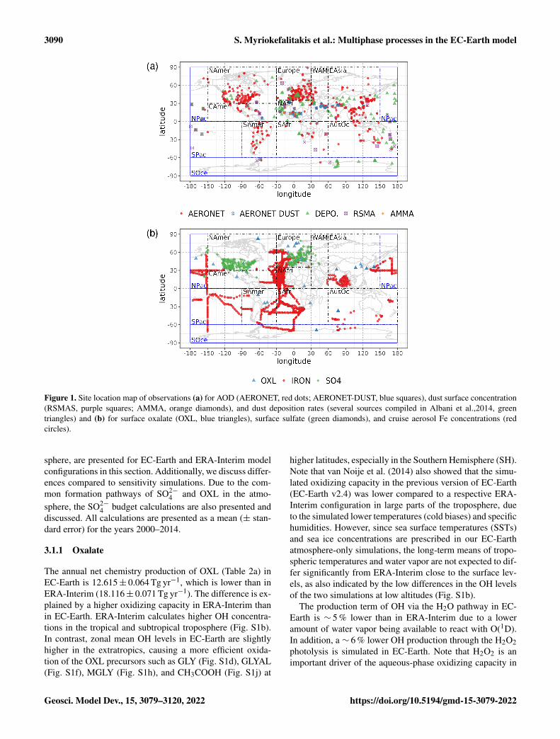
Figure 1. Site location map of observations (a) for AOD (AERONET, red dots; AERONET-DUST, blue squares), dust surface concentration(RSMAS, purple squares; AMMA, orange diamonds), and dust deposition rates (several sources compiled in Albani et al.,2014, greentriangles) and (b) for surface oxalate (OXL, blue triangles), surface sulfate (green diamonds), and cruise aerosol Fe concentrations (redcircles).
sphere, are presented for EC-Earth and ERA-Interim modelconfigurations in this section. Additionally, we discuss differ-ences compared to sensitivity simulations. Due to the com-mon formation pathways of SO2−
4 and OXL in the atmo-sphere, the SO2−
4 budget calculations are also presented anddiscussed. All calculations are presented as a mean (± stan-dard error) for the years 2000–2014.
3.1.1 Oxalate
The annual net chemistry production of OXL (Table 2a) inEC-Earth is 12.615± 0.064 Tg yr−1, which is lower than inERA-Interim (18.116± 0.071 Tg yr−1). The difference is ex-plained by a higher oxidizing capacity in ERA-Interim thanin EC-Earth. ERA-Interim calculates higher OH concentra-tions in the tropical and subtropical troposphere (Fig. S1b).In contrast, zonal mean OH levels in EC-Earth are slightlyhigher in the extratropics, causing a more efficient oxida-tion of the OXL precursors such as GLY (Fig. S1d), GLYAL(Fig. S1f), MGLY (Fig. S1h), and CH3COOH (Fig. S1j) at
higher latitudes, especially in the Southern Hemisphere (SH).Note that van Noije et al. (2014) also showed that the simu-lated oxidizing capacity in the previous version of EC-Earth(EC-Earth v2.4) was lower compared to a respective ERA-Interim configuration in large parts of the troposphere, dueto the simulated lower temperatures (cold biases) and specifichumidities. However, since sea surface temperatures (SSTs)and sea ice concentrations are prescribed in our EC-Earthatmosphere-only simulations, the long-term means of tropo-spheric temperatures and water vapor are not expected to dif-fer significantly from ERA-Interim close to the surface lev-els, as also indicated by the low differences in the OH levelsof the two simulations at low altitudes (Fig. S1b).
The production term of OH via the H2O pathway in EC-Earth is ∼ 5 % lower than in ERA-Interim due to a loweramount of water vapor being available to react with O(1D).In addition, a ∼ 6 % lower OH production through the H2O2photolysis is simulated in EC-Earth. Note that H2O2 is animportant driver of the aqueous-phase oxidizing capacity in
Geosci. Model Dev., 15, 3079–3120, 2022 https://doi.org/10.5194/gmd-15-3079-2022

S. Myriokefalitakis et al.: Multiphase processes in the EC-Earth model 3091
Table 2. Global budgets, atmospheric burdens, and lifetimes, averaged for the period 2000–2014, of (a) oxalate (OXL), (b) sulfate, anddissolved Fe-containing aerosols from (c) combustion processes (FeC) and (d) mineral dust (FeD) for EC-Earth, ERA-Interim, and ERA-Interim(sens) simulations.
EC-Earth Era-Interim Era-Interim(sens)
(a) Oxalate
Emissions (Tg yr−1) 0.373Chemistry production (Tg yr−1)– GLYOLI+OH 10.597 14.764 –– MGLY+OH 1.079 1.415 1.552– GLX+OH/NO3 3.369 4.618 9.962Chemistry loss (Tg yr−1)– OXL+OH/NO3 1.019 1.189 0.822– [Fe(OXL)2]−+hv 1.412 1.475 0.680Deposition (Tg yr−1)– Dry deposition 0.134 0.176 0.097– Wet scavenging 12.850 18.313 10.286Atmospheric burden (Tg) 0.219 0.330 0.189Lifetime (d) 5.175 5.691 5.810
(b) Sulfate
Emissions (Tg S yr−1) 1.593H2SO4 chemistry production (Tg S yr−1)– SO2+OH 11.976 11.088S(VI) chemistry production (Tg S yr−1)– S(IV)+H2O2 32.902 35.812– S(IV)+O3 5.927 4.760– S(IV)+HO2 0.004 0.004– S(IV)+CH3O2H 0.051 0.049Deposition (Tg S yr−1)– Dry deposition 3.079 2.912– Wet scavenging 49.368 50.394Atmospheric burden (Tg S) 0.692 0.961Lifetime (d) 4.816 6.579
(c) Dissolved FeC
Emissions (Tg yr−1) 0.012Dissolution (Tg yr−1)– FeC+H+ 0.047 0.049 0.049– FeC+OXL 0.182 0.188 0.183– FeC+hv 0.045 0.047 0.046Deposition (Tg yr−1)– Dry deposition 0.081 0.080 0.077– Wet scavenging 0.206 0.217 0.212Atmospheric burden (Tg) 0.002 0.003 0.003Lifetime (d) 2.970 4.163 4.203
(d) Dissolved FeD
Emissions (Tg yr−1) 0.059 0.049 0.049Dissolution (Tg yr−1)– FeD+H+ 0.315 0.311 0.311– FeD+OXL 0.170 0.168 0.164– FeD+hv 0.047 0.049 0.048Deposition (Tg yr−1)– Dry deposition 0.140 0.132 0.130– Wet scavenging 0.452 0.446 0.441Atmospheric burden (Tg) 0.006 0.010 0.010Lifetime (d) 3.837 6.236 6.264
https://doi.org/10.5194/gmd-15-3079-2022 Geosci. Model Dev., 15, 3079–3120, 2022

3092 S. Myriokefalitakis et al.: Multiphase processes in the EC-Earth model
the model, with about 80 % of the OH radicals in the liquidphase being produced by photolysis of the dissolved H2O2.In more detail, the lower atmospheric abundance of the gas-phase H2O2 in EC-Earth (∼ 11 %) leads to smaller H2O2uptake in the aqueous phase (∼ 13 %) and thus to a sloweroxidation of OXL precursors due to the respective lower dis-solved OH radical production (∼ 19 %). Overall, the total OHproduction is ∼ 7 % lower in EC-Earth, which correspondsto a ∼ 18 % lower aqueous-phase OH production, resultingin a ∼ 30 % lower OXL net chemistry production comparedto ERA-Interim.
The total OXL production is 15.5 Tg yr−1 in Lin etal. (2014) and 14.5 Tg yr−1 in Liu et al. (2012), both ofthese values are lower than our ERA-Interim estimates(20.8 Tg yr−1; Table 2a) but close to EC-Earth (15.0 Tg yr−1;Table 2a). The main reason for the lower chemistry pro-duction of other published estimates compared to our re-sults is the contribution of the aqueous-phase glyoxal ox-idation scheme proposed by Carlton et al. (2007) that isapplied in our simulations. The oxidation of the glyoxal-derived high-molecular-weight products formed mainly inthe cloud droplets is calculated to contribute significantly tothe global OXL production in our model (Table 2a). This re-sult is in line with Carlton et al. (2007), who indicated thatthe GLX pathway may not be the primary pathway for ox-alic acid formation, but this is instead attributed to the rapidoxidation of GLY multifunctional products via the OH rad-icals (i.e., 3.1× 10¹⁰ L mol−1 s−1; Table S2). However, forERA-Interim(sens), where no such reactions are considered,the total OXL chemical production is calculated on average11.5 Tg yr−1 (Table 2); i.e., closer to the estimates of Lin etal. (2014) and Liu et al. (2012). On the other hand, our ERA-Interim net chemistry production calculations are close to theestimates of Myriokefalitakis et al. (2011) (i.e., 21.2 Tg yr−1)when no potential effects of the ionic strength (e.g., Her-rmann, 2003) on OXL precursors are considered, althoughthis is still lower since no Fe chemistry was considered inthat latter study. Indeed, the enhanced aqueous-phase oxida-tion capacity due to the Fenton reaction increases both theproduction and the destruction terms of OXL in our model,leading to ∼ 7 % lower net OXL production and a lower(∼ 8 %) atmospheric abundance, respectively. Nonetheless,our calculations indicate that Fe chemistry impacts on OXLnet production drastically, increasing the destruction of thedissolved oxalic acid by at least ∼ 50 %. The potential pri-mary sources (0.373± 0.005 Tg yr−1) accounted for in themodel (Table 2a) do not, however, significantly contributeto the simulated OXL atmospheric levels, and only a smallfraction of OXL is calculated to be formed in aerosol water(∼ 6 %) for all simulations in this work.
Focusing further on the atmospheric sinks of OXL,roughly 13 % in ERA-Interim and 16 % in EC-Earth of theproduced oxalic acid is oxidized into CO2 in the aqueousphase, mainly via the photolysis of the [Fe(OXL)2]− com-plex (∼ 55 %) and via OH radicals (∼ 45 %). The fraction
of the total produced OXL that is destroyed in the aqueous-phase is higher than in Liu et al. (2012) by ∼ 7 %, whereno Fe chemistry was considered, but lower compared toLin et al. (2014) and Myriokefalitakis et al. (2011), whereroughly 30 % of the produced OXL is oxidized into CO2 inthe aqueous phase. Finally, a total average deposition rate of18.5 Tg yr−1 is calculated in ERA-Interim, primarily due towet scavenging (∼ 99 %), resulting in a global atmosphericlifetime of 5.7 d, which is close to Liu et al. (2012) andLin et al. (2014) but higher compared to Myriokefalitakis etal. (2011) (∼ 3 d); this is probably because of the more in-tense OXL production at higher altitudes in our model.
The major pathways of global OXL production, both inERA-Interim and EC-Earth, are the oxidation of glyoxal(∼ 74 %), followed by glycolaldehyde (∼ 11 %), methylgly-oxal (∼ 8 %), and acetic acid (∼ 7 %). Glyoxylic acid is nev-ertheless an important intermediate species because it is di-rectly converted to OXL in the aqueous phase upon oxida-tion. Other important findings concerning the chemical bud-gets are summarized below.
1. Glyoxal. About 70 Tg yr−1 GLY is produced in the gas-phase in ERA-Interim, similar to Lin et al. (2014), whilein EC-Earth it is calculated 3 % lower. The global gas-phase production of the present work is higher thanother global model estimates, e.g., about 56 Tg yr−1
(Myriokefalitakis et al., 2008), 40 Tg yr−1 (Fu et al.,2009, 2008), and 21 Tg yr−1 (Liu et al., 2012). Thisdifference can be explained by the more comprehen-sive isoprene chemistry of the gas-phase scheme usedhere (Myriokefalitakis et al., 2020b). Indeed, isoprenesecondary oxidation products (e.g., epoxides) are sig-nificant precursors of GLY in the atmosphere (Knoteet al., 2014) and the contribution of isoprene epoxides(IEPOX) from the gas-phase isoprene oxidation is hereconsidered as a pathway of GLY formation. Note thatthe oxidation of other biogenic hydrocarbons, like ter-penes and other reactive organics, may also result inGLY formation, since their chemistry is lumped on thefirst-generation peroxy radicals of isoprene in the model(Myriokefalitakis et al., 2020b). Besides the biogenichydrocarbon oxidation, the model considers GLY for-mation due to the oxidation of other organic species(e.g., Warneck, 2003), such as acetylene (4.8 Tg yr−1)and aromatics (18.8 Tg yr−1). In the gas phase, otherhydrocarbons, like ethene, further contribute to the at-mospheric production of GLY via their oxidation prod-ucts, mainly glycolaldehyde (5.4 Tg yr−1). However, asin many modeling studies, additional primary and/orsecondary glyoxal sources might be still missing in ourmodel. Indeed, the elevated glyoxal concentrations overoceans that have been observed from space (e.g., Wit-trock et al., 2006) would require at least 20 Tg yr−1
of extra marine sources to reconcile model simula-tions with satellite retrievals (Myriokefalitakis et al.,
Geosci. Model Dev., 15, 3079–3120, 2022 https://doi.org/10.5194/gmd-15-3079-2022
S. Myriokefalitakis et al.: Multiphase processes in the EC-Earth model 3093
2008). Great uncertainties, however, still exist on theseoceanic sources (Alvarado et al., 2020; Sinreich et al.,2010), and therefore the only glyoxal primary sourcesaccounted for in the model are from biofuel combus-tion and biomass burning processes (e.g., Christian etal., 2003; Fu et al., 2008; Hays et al., 2002), overallresulting in about 7 Tg yr−1 on average in the model(Myriokefalitakis et al., 2020b). Glyoxal is rapidly de-stroyed in the atmosphere via photolysis (∼ 70 %), fol-lowed by its oxidation in the gas phase (∼ 15 %) and theaqueous phase (∼ 15 %). Roughly 5.4 Tg yr−1 of gly-oxal is produced in the aqueous phase via the dissolvedGLYAL oxidation in ERA-Interim, close to the Liu etal. (2012) calculations but somehow higher comparedto EC-Earth. Overall, the net cloud uptake of glyoxalin ERA-Interim is 6.3 Tg yr−1, which is higher than theestimates from Liu et al. (2012) (1.6 Tg yr−1). As ex-pected, this increase is due to the applied glyoxal oxi-dation scheme in the aqueous phase of our base simu-lations. Finally, 4.2 Tg yr−1 of glyoxal is removed fromthe atmosphere via wet scavenging (∼ 73 %) and dry de-position (∼ 27 %).
2. Glycolaldehyde. GLYAL is also a significant species forOXL atmospheric abundance since its oxidation directlyproduces GLY both in the gas and the aqueous phase. InERA-Interim, the gas-phase production is 92.5 Tg yr−1
on a global scale, with the primary sources accountingfor 5.4 Tg yr−1 (Myriokefalitakis et al., 2020b) on av-erage. In EC-Earth, the gas-phase production is ∼ 1 %lower. GLYAL is destroyed via gas-phase photolysis(∼ 55 %) and by OH radicals in the gas phase (∼ 35 %)and the aqueous phase (∼ 10 %). Ethene oxidation prod-ucts contribute ∼ 39 % to GLYAL production, but iso-prene chemistry dominates its chemical production inthe model. The only source of GLYAL in the aqueousphase is nevertheless the transfer from the gas phase.The dissolved GLYAL is oxidized to produce GLY(∼ 60 %) and GLX (∼ 40 %), overall resulting in a netaqueous uptake of 8.3 Tg yr−1 in ERA-Interim, close tothe estimates of Liu et al. (2012), but almost 40 % higherthan in Lin et al. (2014). This higher uptake of GLYALin the aqueous phase is due to the respective higher(∼ 14 %) gas-phase production in our model. Note thatin ERA-Interim the net aqueous uptake of GLYAL iscalculated ∼ 24 % lower compared to ERA-Interim.
3. Methylglyoxal. The global annual mean gas-phase pro-duction of MGLY in ERA-Interim is 237 Tg yr−1
on average, with the primary sources accounting for4.6 Tg yr−1. The gas-phase production is higher thanthe 160–169 Tg yr−1 reported by other modeling studies(Fu et al., 2008; Lin et al., 2014; Liu et al., 2012) ow-ing to the contribution of oxidation products consideredin the gas-phase isoprene chemistry scheme (Myrioke-falitakis et al., 2020b). Roughly 56 % of MGLY is pro-
duced via the gas-phase oxidation of HYAC with OHradicals, which is lower than the estimated ∼ 75 % inFu et al. (2008). The remaining MGLY production isdue to isoprene oxidation products, i.e., ∼ 10 % fromIEPOX oxidation, and ∼ 7 % from methyl vinyl ke-tone (MVK) and methacrolein (MACR) oxidation. Inthe aqueous phase, MGLY is produced via the dissolvedHYAC oxidation (13.0 Tg yr−1) and then further oxi-dized by OH radicals (11.6 Tg yr−1) into pyruvic acid(PRV), methylglyoxal oligomers (MGLYOLI), and to alesser extent into GLX. Note that the calculated con-tribution of dissolved HYAC to the aqueous-phase pro-duction of MGLY is higher compared to the nearly neg-ligible rates in Liu et al. (2012) because of the highergas-phase production of HYAC in our model. MGLYis chemically destroyed in the model mainly by gas-phase photolysis (∼ 60 %), the OH radicals in the gasphase (∼ 35 %), and via oxidation in the aqueous phase(∼ 5 %).
4. Pyruvic and acetic acids. The chemical production ofPRV is 14.7 Tg yr−1 in ERA-Interim and 16.7 Tg yr−1
in EC-Earth. PRV is mainly produced by terpene ox-idation via O3 (∼ 51 %) in the gas phase followed bymethyl vinyl ketone (MVK) oxidation (∼ 5 %). In theaqueous phase, PRV is solely produced from MGLYoxidation (6.5 Tg yr−1) and subsequently oxidized toCH3COOH. PRV is mainly removed via photolysis inthe gas phase and via oxidation by OH radicals in theaqueous phase (∼ 30 %). However, more than half of theproduced PRV in the aqueous phase directly contributesto the SOA mass of the model upon cloud evaporation.The gas-phase production of acetic acid is 44.3 Tg yr−1,with the primary sources accounting for approximately23.9 Tg yr−1. In the aqueous phase, roughly 3 Tg yr−1
of CH3COOH is produced via PRV oxidation. Note thatthe net uptake of CH3COOH (0.7 Tg yr−1) is calculatedin the model similar to the Lin et al. (2014) estimatesbut smaller than the 6.7 Tg yr−1 calculated by Liu etal. (2012).
5. Glyoxylic acid. The GLX production rate is 7.1 Tg yr−1
in EC-Earth and is ∼ 30 % lower in ERA-Interim.About 55 % of the produced GLX is directly oxidizedto oxalic acid in the aqueous phase and ∼ 25 % isadded directly to the SOA pool. Upon cloud evapora-tion, part of the produced GLX is also transferred in thegas phase, where it is either oxidized by OH radicals(∼ 60 %), photolyzed (∼ 33 %), or deposited (∼ 7 %).Due to the destruction of GLX in the gas phase, its totalproduction is lower (∼ 60 %) compared to the produc-tion estimates in Lin et al. (2014) and Liu et al. (2012).For the EC-Earth and ERA-Interim, most of the pro-duced GLX in the aqueous phase is derived from theoxidation of GLYAL (∼ 48 %), followed by the oxi-dation of CH3COOH (30 %), GLY and its oligomeric
https://doi.org/10.5194/gmd-15-3079-2022 Geosci. Model Dev., 15, 3079–3120, 2022
3094 S. Myriokefalitakis et al.: Multiphase processes in the EC-Earth model
products (∼ 15 %), and MGLY. The relative contribu-tions in our calculations differ from the estimates inLin et al. (2014), where GLX is primarily produced byGLY oxidation (∼ 77 %) followed by GLYAL (∼ 14 %),MGLY (∼ 1 %), and acetic acid (∼ 8 %). These dif-ferences are also caused by the direct contribution ofthe GLY oxidation products to the OXL formation. Onthe other hand, in the ERA-Interim(sens) simulationthe calculated fractions agree well with other publishedestimates, where GLY overall dominates (∼ 60 %) theGLX production in the aqueous phase.
Figure 2a presents the annual mean (average 2000–2014)net chemistry production rates of OXL in EC-Earth and therespective absolute differences compared to ERA-interim(Fig. 2c). The maximum OXL production rates are calcu-lated around the tropics and in the Southern Hemisphere,where both biogenic emissions (mainly isoprene) and the liq-uid cloud water are substantially enhanced (Fig. S2a). TheAmazon region appears as the largest source of OXL, alongwith central Africa and Southeast Asia. At higher latitudes(>45◦ N) the lower cloud liquid water content and vegeta-tion cover lead to a lower OXL production over Asia andNorth America. However, over highly populated regions inthe Northern Hemisphere, such as in Europe, the US, andChina, enhanced OXL production rates are calculated dueto its anthropogenic precursors. Furthermore, a significantsource of OXL is calculated downwind of land areas, suchas the South Pacific and the tropical Atlantic Ocean due tothe long-range transport of OXL precursors.
The illustrated differences in OXL production betweenERA-interim and EC-Earth (Fig. 2c) are caused due to theadopted atmospheric dynamics (i.e., online calculated ver-sus offline), as both simulations use identical prescribed an-thropogenic and biogenic emissions (see van Noije et al.,2021). For instance, EC-Earth calculates higher cloud waterconcentrations at ∼ 800–600 hPa around the tropics (30◦ S–30◦ N) compared to ERA-Interim. In contrast, lower concen-trations are derived aloft, with ERA-Interim presenting en-hanced cloud water concentrations at ∼ 400 hPa (Fig. S2b).Moreover, due to the lower OH concentrations in the tropicaland subtropical troposphere (Fig. S1b), EC-Earth gives lowerOXL production rates, especially over intense biogenic emis-sion areas. Overall, the difference in the oxidizing capacity ofthe atmosphere between the two configurations significantlyimpacts the aqueous-phase OXL production efficiency in themodel.
3.1.2 Sulfate
Sulfate (SO2−4 ) is the main inorganic aerosol species pro-
duced in the aqueous phase, and similar to OXL its produc-tion in the model mainly occurs in cloud droplets. In addi-tion, these two species largely reside in the aerosol accu-mulation mode of the model (roughly 99 % for SO−2
4 and
97 % for OXL). SO2−4 is a key species for determining at-
mospheric acidity, and therefore here we also present thesulfate budget in conjunction with that of OXL. Sulfate isproduced both in cloud droplets and in aerosol water, withthe production in aerosol water having a negligible contri-bution on a global scale. In contrast to OXL, for which nogas-phase production is considered, the gas-phase oxidationof SO2 via OH radicals contributes to the total SO2−
4 con-centrations with about 12.0 Tg S yr−1 (Table 2b). Our globalestimate of the gaseous sulfuric acid (H2SO4) productionis higher than in EC-Earth v2.4 (7.8 Tg S yr−1 averaged forthe years 2000–2009; van Noije et al., 2014) but slightlylower than in the EC-Earth3-AerChem AMIP simulations(van Noije et al., 2021) used for the CMIP6 experiments(available in https://esg-dn1.nsc.liu.se/search/cmip6-liu/, lastaccess: 11 June 2021) where 12.9 Tg S yr−1 of H2SO4 areproduced (averaged for the years 2000–2014). These differ-ences can be directly attributed to the OH radical produc-tion rates in the gas phase between the new and the previ-ous chemistry versions of the atmospheric model, as havebeen discussed in Myriokefalitakis et al. (2020b). Despite thegenerally lower gas-phase OH radical levels (Fig. S1b), theslightly higher (∼ 8 %) global H2SO4 gas-phase productionrate in EC-Earth than in ERA-Interim (Table 2b) can be at-tributed to the higher (∼ 6%) DMS emissions in EC-Earth(Fig. S4b) that contribute to the atmospheric SO2 levels overthe ocean.
The aqueous-phase SO2−4 chemistry production from
the oxidation of dissolved SO2 is 39.8 Tg S yr−1 in EC-Earth (Table 2b), which is higher than in EC-Earth v2.4(29.3 Tg S yr−1; van Noije et al., 2014) and EC-Earth3-AerChem (32.5 Tg S yr−1). The higher SO2−
4 chemical pro-duction is mainly due to the higher SO2 aqueous-phase oxi-dation rates by H2O2. In more detail, our calculations showthat ∼ 84 % of the global SO2−
4 production in EC-Earth isdue to the dissolved SO2 oxidation via H2O2; 33.3 Tg S yr−1
is produced due to H2O2, which is higher compared to23.9 Tg S yr−1 in van Noije et al. (2014). The dissolvedSO2 oxidation via O3 (6.4 Tg S yr−1) is also higher than inEC-Earth v2.4 (5.4 Tg S yr−1). However, the contribution ofCH3O2H to the SO2−
4 aqueous-phase production is small(0.05 Tg S yr−1) in the model, with the HO2 contribution be-ing practically negligible on the global scale (0.02 Tg S yr−1)for all simulations performed in this study. A total annualmean deposition rate of 52.5 Tg S yr−1 is simulated in EC-Earth, with wet scavenging dominating the total depositionrate (∼ 93 %). Note that 2.5 % of the sulfur in the SO2 emis-sions (1.6 Tg S yr−1) is assumed to be in the form of SO2−
4 forall simulations, which accounts for its formation in the sub-grid plumes (Aan de Brugh et al., 2011; Huijnen et al., 2010).Overall, a global SO2−
4 lifetime over deposition of 4.8 d iscalculated in EC-Earth, which is lower than in ERA-Interim(6.6 d) but similar to the EC-Earth v2.4 estimate (4.9 d).
Geosci. Model Dev., 15, 3079–3120, 2022 https://doi.org/10.5194/gmd-15-3079-2022
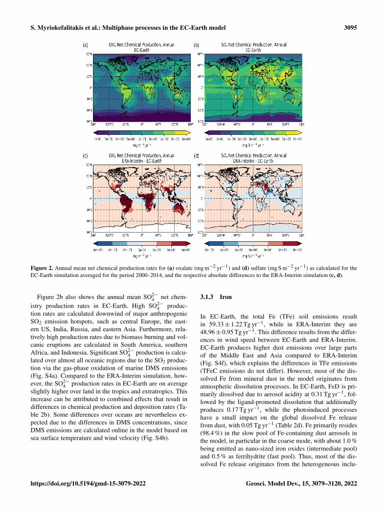
S. Myriokefalitakis et al.: Multiphase processes in the EC-Earth model 3095
Figure 2. Annual mean net chemical production rates for (a) oxalate (mg m−2 yr−1) and (d) sulfate (mg S m−2 yr−1) as calculated for theEC-Earth simulation averaged for the period 2000–2014, and the respective absolute differences to the ERA-Interim simulation (c, d).
Figure 2b also shows the annual mean SO2−4 net chem-
istry production rates in EC-Earth. High SO2−4 produc-
tion rates are calculated downwind of major anthropogenicSO2 emission hotspots, such as central Europe, the east-ern US, India, Russia, and eastern Asia. Furthermore, rela-tively high production rates due to biomass burning and vol-canic eruptions are calculated in South America, southernAfrica, and Indonesia. Significant SO2−
4 production is calcu-lated over almost all oceanic regions due to the SO2 produc-tion via the gas-phase oxidation of marine DMS emissions(Fig. S4a). Compared to the ERA-Interim simulation, how-ever, the SO2−
4 production rates in EC-Earth are on averageslightly higher over land in the tropics and extratropics. Thisincrease can be attributed to combined effects that result indifferences in chemical production and deposition rates (Ta-ble 2b). Some differences over oceans are nevertheless ex-pected due to the differences in DMS concentrations, sinceDMS emissions are calculated online in the model based onsea surface temperature and wind velocity (Fig. S4b).
3.1.3 Iron
In EC-Earth, the total Fe (TFe) soil emissions resultin 59.33± 1.22 Tg yr−1, while in ERA-Interim they are48.96± 0.95 Tg yr−1. This difference results from the differ-ences in wind speed between EC-Earth and ERA-Interim.EC-Earth produces higher dust emissions over large partsof the Middle East and Asia compared to ERA-Interim(Fig. S4f), which explains the differences in TFe emissions(TFeC emissions do not differ). However, most of the dis-solved Fe from mineral dust in the model originates fromatmospheric dissolution processes. In EC-Earth, FeD is pri-marily dissolved due to aerosol acidity at 0.31 Tg yr−1, fol-lowed by the ligand-promoted dissolution that additionallyproduces 0.17 Tg yr−1, while the photoinduced processeshave a small impact on the global dissolved Fe releasefrom dust, with 0.05 Tg yr−1 (Table 2d). Fe primarily resides(98.4 %) in the slow pool of Fe-containing dust aerosols inthe model, in particular in the coarse mode, with about 1.0 %being emitted as nano-sized iron oxides (intermediate pool)and 0.5 % as ferrihydrite (fast pool). Thus, most of the dis-solved Fe release originates from the heterogeneous inclu-
https://doi.org/10.5194/gmd-15-3079-2022 Geosci. Model Dev., 15, 3079–3120, 2022
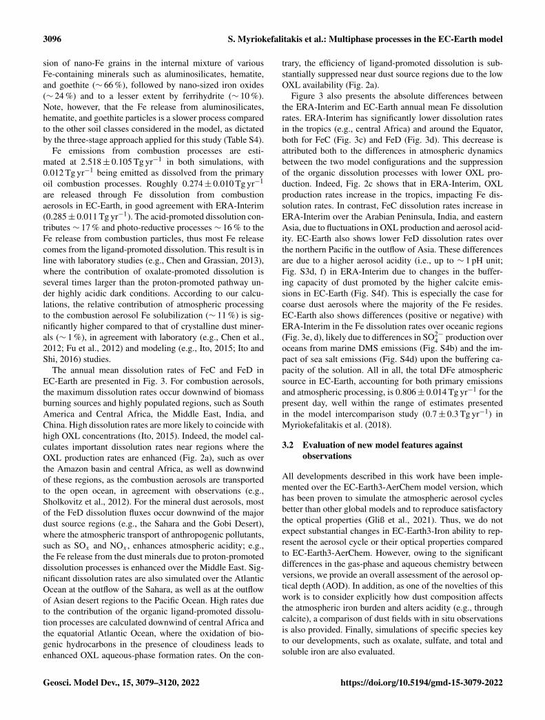
3096 S. Myriokefalitakis et al.: Multiphase processes in the EC-Earth model
sion of nano-Fe grains in the internal mixture of variousFe-containing minerals such as aluminosilicates, hematite,and goethite (∼ 66 %), followed by nano-sized iron oxides(∼ 24 %) and to a lesser extent by ferrihydrite (∼ 10 %).Note, however, that the Fe release from aluminosilicates,hematite, and goethite particles is a slower process comparedto the other soil classes considered in the model, as dictatedby the three-stage approach applied for this study (Table S4).
Fe emissions from combustion processes are esti-mated at 2.518± 0.105 Tg yr−1 in both simulations, with0.012 Tg yr−1 being emitted as dissolved from the primaryoil combustion processes. Roughly 0.274± 0.010 Tg yr−1
are released through Fe dissolution from combustionaerosols in EC-Earth, in good agreement with ERA-Interim(0.285± 0.011 Tg yr−1). The acid-promoted dissolution con-tributes ∼ 17 % and photo-reductive processes ∼ 16 % to theFe release from combustion particles, thus most Fe releasecomes from the ligand-promoted dissolution. This result is inline with laboratory studies (e.g., Chen and Grassian, 2013),where the contribution of oxalate-promoted dissolution isseveral times larger than the proton-promoted pathway un-der highly acidic dark conditions. According to our calcu-lations, the relative contribution of atmospheric processingto the combustion aerosol Fe solubilization (∼ 11 %) is sig-nificantly higher compared to that of crystalline dust miner-als (∼ 1 %), in agreement with laboratory (e.g., Chen et al.,2012; Fu et al., 2012) and modeling (e.g., Ito, 2015; Ito andShi, 2016) studies.
The annual mean dissolution rates of FeC and FeD inEC-Earth are presented in Fig. 3. For combustion aerosols,the maximum dissolution rates occur downwind of biomassburning sources and highly populated regions, such as SouthAmerica and Central Africa, the Middle East, India, andChina. High dissolution rates are more likely to coincide withhigh OXL concentrations (Ito, 2015). Indeed, the model cal-culates important dissolution rates near regions where theOXL production rates are enhanced (Fig. 2a), such as overthe Amazon basin and central Africa, as well as downwindof these regions, as the combustion aerosols are transportedto the open ocean, in agreement with observations (e.g.,Sholkovitz et al., 2012). For the mineral dust aerosols, mostof the FeD dissolution fluxes occur downwind of the majordust source regions (e.g., the Sahara and the Gobi Desert),where the atmospheric transport of anthropogenic pollutants,such as SOx and NOx , enhances atmospheric acidity; e.g.,the Fe release from the dust minerals due to proton-promoteddissolution processes is enhanced over the Middle East. Sig-nificant dissolution rates are also simulated over the AtlanticOcean at the outflow of the Sahara, as well as at the outflowof Asian desert regions to the Pacific Ocean. High rates dueto the contribution of the organic ligand-promoted dissolu-tion processes are calculated downwind of central Africa andthe equatorial Atlantic Ocean, where the oxidation of bio-genic hydrocarbons in the presence of cloudiness leads toenhanced OXL aqueous-phase formation rates. On the con-
trary, the efficiency of ligand-promoted dissolution is sub-stantially suppressed near dust source regions due to the lowOXL availability (Fig. 2a).
Figure 3 also presents the absolute differences betweenthe ERA-Interim and EC-Earth annual mean Fe dissolutionrates. ERA-Interim has significantly lower dissolution ratesin the tropics (e.g., central Africa) and around the Equator,both for FeC (Fig. 3c) and FeD (Fig. 3d). This decrease isattributed both to the differences in atmospheric dynamicsbetween the two model configurations and the suppressionof the organic dissolution processes with lower OXL pro-duction. Indeed, Fig. 2c shows that in ERA-Interim, OXLproduction rates increase in the tropics, impacting Fe dis-solution rates. In contrast, FeC dissolution rates increase inERA-Interim over the Arabian Peninsula, India, and easternAsia, due to fluctuations in OXL production and aerosol acid-ity. EC-Earth also shows lower FeD dissolution rates overthe northern Pacific in the outflow of Asia. These differencesare due to a higher aerosol acidity (i.e., up to ∼ 1 pH unit;Fig. S3d, f) in ERA-Interim due to changes in the buffer-ing capacity of dust promoted by the higher calcite emis-sions in EC-Earth (Fig. S4f). This is especially the case forcoarse dust aerosols where the majority of the Fe resides.EC-Earth also shows differences (positive or negative) withERA-Interim in the Fe dissolution rates over oceanic regions(Fig. 3e, d), likely due to differences in SO2−
4 production overoceans from marine DMS emissions (Fig. S4b) and the im-pact of sea salt emissions (Fig. S4d) upon the buffering ca-pacity of the solution. All in all, the total DFe atmosphericsource in EC-Earth, accounting for both primary emissionsand atmospheric processing, is 0.806± 0.014 Tg yr−1 for thepresent day, well within the range of estimates presentedin the model intercomparison study (0.7± 0.3 Tg yr−1) inMyriokefalitakis et al. (2018).
3.2 Evaluation of new model features againstobservations
All developments described in this work have been imple-mented over the EC-Earth3-AerChem model version, whichhas been proven to simulate the atmospheric aerosol cyclesbetter than other global models and to reproduce satisfactorythe optical properties (Gliß et al., 2021). Thus, we do notexpect substantial changes in EC-Earth3-Iron ability to rep-resent the aerosol cycle or their optical properties comparedto EC-Earth3-AerChem. However, owing to the significantdifferences in the gas-phase and aqueous chemistry betweenversions, we provide an overall assessment of the aerosol op-tical depth (AOD). In addition, as one of the novelties of thiswork is to consider explicitly how dust composition affectsthe atmospheric iron burden and alters acidity (e.g., throughcalcite), a comparison of dust fields with in situ observationsis also provided. Finally, simulations of specific species keyto our developments, such as oxalate, sulfate, and total andsoluble iron are also evaluated.
Geosci. Model Dev., 15, 3079–3120, 2022 https://doi.org/10.5194/gmd-15-3079-2022
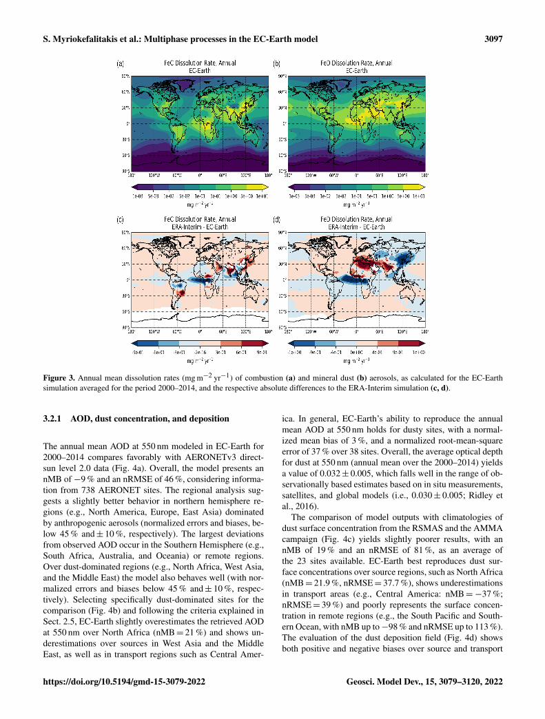
S. Myriokefalitakis et al.: Multiphase processes in the EC-Earth model 3097
Figure 3. Annual mean dissolution rates (mg m−2 yr−1) of combustion (a) and mineral dust (b) aerosols, as calculated for the EC-Earthsimulation averaged for the period 2000–2014, and the respective absolute differences to the ERA-Interim simulation (c, d).
3.2.1 AOD, dust concentration, and deposition
The annual mean AOD at 550 nm modeled in EC-Earth for2000–2014 compares favorably with AERONETv3 direct-sun level 2.0 data (Fig. 4a). Overall, the model presents annMB of −9 % and an nRMSE of 46 %, considering informa-tion from 738 AERONET sites. The regional analysis sug-gests a slightly better behavior in northern hemisphere re-gions (e.g., North America, Europe, East Asia) dominatedby anthropogenic aerosols (normalized errors and biases, be-low 45 % and± 10 %, respectively). The largest deviationsfrom observed AOD occur in the Southern Hemisphere (e.g.,South Africa, Australia, and Oceania) or remote regions.Over dust-dominated regions (e.g., North Africa, West Asia,and the Middle East) the model also behaves well (with nor-malized errors and biases below 45 % and± 10 %, respec-tively). Selecting specifically dust-dominated sites for thecomparison (Fig. 4b) and following the criteria explained inSect. 2.5, EC-Earth slightly overestimates the retrieved AODat 550 nm over North Africa (nMB= 21 %) and shows un-derestimations over sources in West Asia and the MiddleEast, as well as in transport regions such as Central Amer-
ica. In general, EC-Earth’s ability to reproduce the annualmean AOD at 550 nm holds for dusty sites, with a normal-ized mean bias of 3 %, and a normalized root-mean-squareerror of 37 % over 38 sites. Overall, the average optical depthfor dust at 550 nm (annual mean over the 2000–2014) yieldsa value of 0.032± 0.005, which falls well in the range of ob-servationally based estimates based on in situ measurements,satellites, and global models (i.e., 0.030± 0.005; Ridley etal., 2016).
The comparison of model outputs with climatologies ofdust surface concentration from the RSMAS and the AMMAcampaign (Fig. 4c) yields slightly poorer results, with annMB of 19 % and an nRMSE of 81 %, as an average ofthe 23 sites available. EC-Earth best reproduces dust sur-face concentrations over source regions, such as North Africa(nMB= 21.9 %, nRMSE= 37.7 %), shows underestimationsin transport areas (e.g., Central America: nMB=−37 %;nRMSE= 39 %) and poorly represents the surface concen-tration in remote regions (e.g., the South Pacific and South-ern Ocean, with nMB up to−98 % and nRMSE up to 113 %).The evaluation of the dust deposition field (Fig. 4d) showsboth positive and negative biases over source and transport
https://doi.org/10.5194/gmd-15-3079-2022 Geosci. Model Dev., 15, 3079–3120, 2022
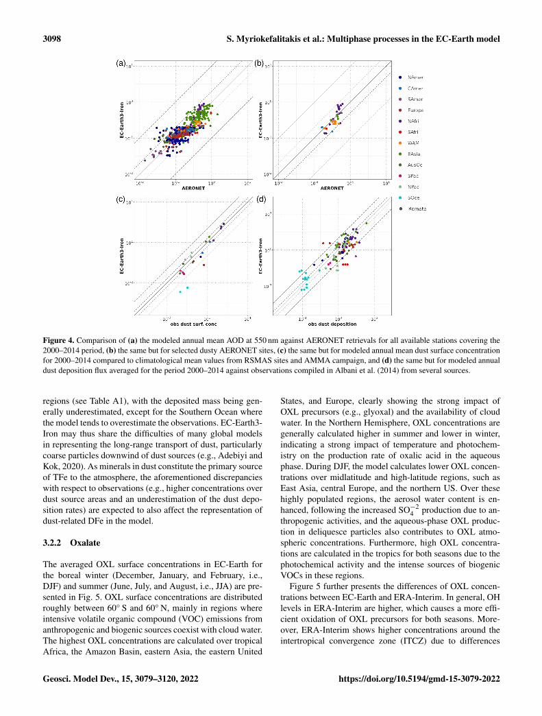
3098 S. Myriokefalitakis et al.: Multiphase processes in the EC-Earth model
Figure 4. Comparison of (a) the modeled annual mean AOD at 550 nm against AERONET retrievals for all available stations covering the2000–2014 period, (b) the same but for selected dusty AERONET sites, (c) the same but for modeled annual mean dust surface concentrationfor 2000–2014 compared to climatological mean values from RSMAS sites and AMMA campaign, and (d) the same but for modeled annualdust deposition flux averaged for the period 2000–2014 against observations compiled in Albani et al. (2014) from several sources.
regions (see Table A1), with the deposited mass being gen-erally underestimated, except for the Southern Ocean wherethe model tends to overestimate the observations. EC-Earth3-Iron may thus share the difficulties of many global modelsin representing the long-range transport of dust, particularlycoarse particles downwind of dust sources (e.g., Adebiyi andKok, 2020). As minerals in dust constitute the primary sourceof TFe to the atmosphere, the aforementioned discrepancieswith respect to observations (e.g., higher concentrations overdust source areas and an underestimation of the dust depo-sition rates) are expected to also affect the representation ofdust-related DFe in the model.
3.2.2 Oxalate
The averaged OXL surface concentrations in EC-Earth forthe boreal winter (December, January, and February, i.e.,DJF) and summer (June, July, and August, i.e., JJA) are pre-sented in Fig. 5. OXL surface concentrations are distributedroughly between 60◦ S and 60◦ N, mainly in regions whereintensive volatile organic compound (VOC) emissions fromanthropogenic and biogenic sources coexist with cloud water.The highest OXL concentrations are calculated over tropicalAfrica, the Amazon Basin, eastern Asia, the eastern United
States, and Europe, clearly showing the strong impact ofOXL precursors (e.g., glyoxal) and the availability of cloudwater. In the Northern Hemisphere, OXL concentrations aregenerally calculated higher in summer and lower in winter,indicating a strong impact of temperature and photochem-istry on the production rate of oxalic acid in the aqueousphase. During DJF, the model calculates lower OXL concen-trations over midlatitude and high-latitude regions, such asEast Asia, central Europe, and the northern US. Over thesehighly populated regions, the aerosol water content is en-hanced, following the increased SO−2
4 production due to an-thropogenic activities, and the aqueous-phase OXL produc-tion in deliquesce particles also contributes to OXL atmo-spheric concentrations. Furthermore, high OXL concentra-tions are calculated in the tropics for both seasons due to thephotochemical activity and the intense sources of biogenicVOCs in these regions.
Figure 5 further presents the differences of OXL concen-trations between EC-Earth and ERA-Interim. In general, OHlevels in ERA-Interim are higher, which causes a more effi-cient oxidation of OXL precursors for both seasons. More-over, ERA-Interim shows higher concentrations around theintertropical convergence zone (ITCZ) due to differences
Geosci. Model Dev., 15, 3079–3120, 2022 https://doi.org/10.5194/gmd-15-3079-2022

S. Myriokefalitakis et al.: Multiphase processes in the EC-Earth model 3099
Figure 5. Oxalate (OXL) surface concentrations (µg m−3) for the boreal winter (DJF; a) and boreal summer (JJA; b), as simulated for theEC-Earth simulation averaged for the period 2000–2014, and the respective absolute differences to the ERA-Interim simulation for surface(c, d) and zonal mean (e, f).
in meteorology between the two simulations, as discussedabove. During boreal winter, some differences are observedover the subtropics of the Northern Hemisphere. AlthoughOXL concentrations are very low over these latitudes, therelatively strong increase in liquid water that serves as amedium for OXL production, both for clouds (Fig. S2b) inhigher altitudes (∼ 400 hPa) and at the surface for deliques-cent particles (Fig. S2d, e) in the ERA-Interim simulation.In the vertical, OXL concentrations are distributed in themodel from the surface to ∼ 400 hPa with a maximum ataround 900 hPa. The zonal mean differences, however, indi-cate strong increases in the Southern Hemisphere (30◦ S–0◦)during boreal winter (Fig. 5e). Compared to EC-Earth, ERA-Interim calculates higher OXL concentrations in the upper
troposphere for both seasons (Fig. 5e, f), mostly due to moreefficient transport of OXL precursors by deep convection intothe tropical and extratropical upper troposphere. In the lowerand middle troposphere, higher concentrations are calculatedin ERA-Interim depending on the location and the season.The concentrations in EC-Earth are also lower than in ERA-Interim in the Northern Hemisphere (NH) extratropics duringboreal summer due to a lower chemical production (Fig. 5f).
Figure 6 presents the comparison of the different modelsimulations performed for this work with OXL surface ob-servations. OXL concentrations show a strong seasonal de-pendence, with maxima during the warm season due to theintense photochemical activity combined with the higher pre-cursor abundance. Over the Mediterranean, and specifically
https://doi.org/10.5194/gmd-15-3079-2022 Geosci. Model Dev., 15, 3079–3120, 2022
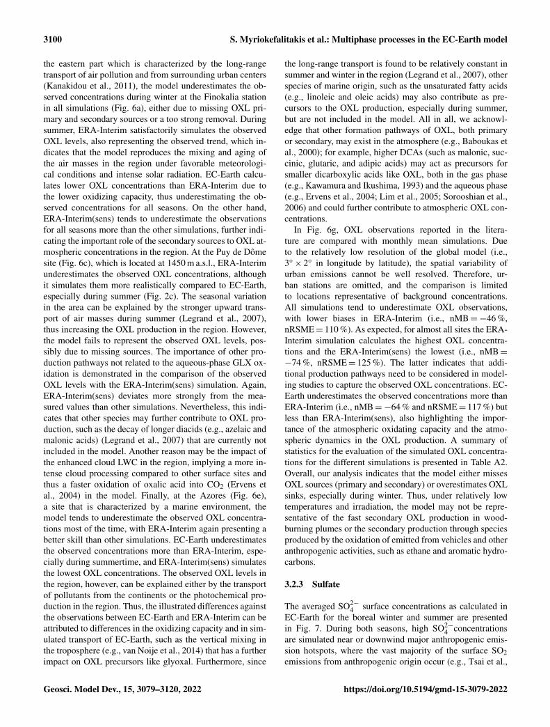
3100 S. Myriokefalitakis et al.: Multiphase processes in the EC-Earth model
the eastern part which is characterized by the long-rangetransport of air pollution and from surrounding urban centers(Kanakidou et al., 2011), the model underestimates the ob-served concentrations during winter at the Finokalia stationin all simulations (Fig. 6a), either due to missing OXL pri-mary and secondary sources or a too strong removal. Duringsummer, ERA-Interim satisfactorily simulates the observedOXL levels, also representing the observed trend, which in-dicates that the model reproduces the mixing and aging ofthe air masses in the region under favorable meteorologi-cal conditions and intense solar radiation. EC-Earth calcu-lates lower OXL concentrations than ERA-Interim due tothe lower oxidizing capacity, thus underestimating the ob-served concentrations for all seasons. On the other hand,ERA-Interim(sens) tends to underestimate the observationsfor all seasons more than the other simulations, further indi-cating the important role of the secondary sources to OXL at-mospheric concentrations in the region. At the Puy de Dômesite (Fig. 6c), which is located at 1450 m a.s.l., ERA-Interimunderestimates the observed OXL concentrations, althoughit simulates them more realistically compared to EC-Earth,especially during summer (Fig. 2c). The seasonal variationin the area can be explained by the stronger upward trans-port of air masses during summer (Legrand et al., 2007),thus increasing the OXL production in the region. However,the model fails to represent the observed OXL levels, pos-sibly due to missing sources. The importance of other pro-duction pathways not related to the aqueous-phase GLX ox-idation is demonstrated in the comparison of the observedOXL levels with the ERA-Interim(sens) simulation. Again,ERA-Interim(sens) deviates more strongly from the mea-sured values than other simulations. Nevertheless, this indi-cates that other species may further contribute to OXL pro-duction, such as the decay of longer diacids (e.g., azelaic andmalonic acids) (Legrand et al., 2007) that are currently notincluded in the model. Another reason may be the impact ofthe enhanced cloud LWC in the region, implying a more in-tense cloud processing compared to other surface sites andthus a faster oxidation of oxalic acid into CO2 (Ervens etal., 2004) in the model. Finally, at the Azores (Fig. 6e),a site that is characterized by a marine environment, themodel tends to underestimate the observed OXL concentra-tions most of the time, with ERA-Interim again presenting abetter skill than other simulations. EC-Earth underestimatesthe observed concentrations more than ERA-Interim, espe-cially during summertime, and ERA-Interim(sens) simulatesthe lowest OXL concentrations. The observed OXL levels inthe region, however, can be explained either by the transportof pollutants from the continents or the photochemical pro-duction in the region. Thus, the illustrated differences againstthe observations between EC-Earth and ERA-Interim can beattributed to differences in the oxidizing capacity and in sim-ulated transport of EC-Earth, such as the vertical mixing inthe troposphere (e.g., van Noije et al., 2014) that has a furtherimpact on OXL precursors like glyoxal. Furthermore, since
the long-range transport is found to be relatively constant insummer and winter in the region (Legrand et al., 2007), otherspecies of marine origin, such as the unsaturated fatty acids(e.g., linoleic and oleic acids) may also contribute as pre-cursors to the OXL production, especially during summer,but are not included in the model. All in all, we acknowl-edge that other formation pathways of OXL, both primaryor secondary, may exist in the atmosphere (e.g., Baboukas etal., 2000); for example, higher DCAs (such as malonic, suc-cinic, glutaric, and adipic acids) may act as precursors forsmaller dicarboxylic acids like OXL, both in the gas phase(e.g., Kawamura and Ikushima, 1993) and the aqueous phase(e.g., Ervens et al., 2004; Lim et al., 2005; Sorooshian et al.,2006) and could further contribute to atmospheric OXL con-centrations.
In Fig. 6g, OXL observations reported in the litera-ture are compared with monthly mean simulations. Dueto the relatively low resolution of the global model (i.e.,3◦× 2◦ in longitude by latitude), the spatial variability ofurban emissions cannot be well resolved. Therefore, ur-ban stations are omitted, and the comparison is limitedto locations representative of background concentrations.All simulations tend to underestimate OXL observations,with lower biases in ERA-Interim (i.e., nMB=−46 %,nRSME= 110 %). As expected, for almost all sites the ERA-Interim simulation calculates the highest OXL concentra-tions and the ERA-Interim(sens) the lowest (i.e., nMB=−74 %, nRSME= 125 %). The latter indicates that addi-tional production pathways need to be considered in model-ing studies to capture the observed OXL concentrations. EC-Earth underestimates the observed concentrations more thanERA-Interim (i.e., nMB=−64 % and nRSME= 117 %) butless than ERA-Interim(sens), also highlighting the impor-tance of the atmospheric oxidating capacity and the atmo-spheric dynamics in the OXL production. A summary ofstatistics for the evaluation of the simulated OXL concentra-tions for the different simulations is presented in Table A2.Overall, our analysis indicates that the model either missesOXL sources (primary and secondary) or overestimates OXLsinks, especially during winter. Thus, under relatively lowtemperatures and irradiation, the model may not be repre-sentative of the fast secondary OXL production in wood-burning plumes or the secondary production through speciesproduced by the oxidation of emitted from vehicles and otheranthropogenic activities, such as ethane and aromatic hydro-carbons.
3.2.3 Sulfate
The averaged SO2−4 surface concentrations as calculated in
EC-Earth for the boreal winter and summer are presentedin Fig. 7. During both seasons, high SO2−
4 concentrationsare simulated near or downwind major anthropogenic emis-sion hotspots, where the vast majority of the surface SO2emissions from anthropogenic origin occur (e.g., Tsai et al.,
Geosci. Model Dev., 15, 3079–3120, 2022 https://doi.org/10.5194/gmd-15-3079-2022

S. Myriokefalitakis et al.: Multiphase processes in the EC-Earth model 3101
Figure 6. Comparison of daily mean observations (black line) of OXL (ng m−3; a, c, e, g) and nss-SO2−4 (µg m−3; b, d, f, h) with the EC-
Earth (orange line and circles) and the ERA-Interim (light blue line and triangles) simulations for Finokalia (Greece) (a), (b) for the periodJuly 2004–July 2006 (Koulouri et al., 2008); for Puy de Dome (France) (c), (d) and Azores (Portugal)(e), (f) for the period September 2002–September 2004 (Legrand et al., 2007); and scatterplot comparisons for observations around the globe (d), (f); the solid line represents the1 : 1 correspondence, and the dashed lines show the 10 : 1 and 1 : 10 relationships, respectively. For completeness, the comparisons for thesensitivity simulation ERA-Interim(sens) for OXL and the EC-Earth(AerChem-AMIP) (green line and squares) for sulfate are also presented.Gray-shaded areas represent the standard deviation of the observations and the color-coded error bars represent the model’s standard error ofthe multi-annual mean for the individual observational period.
https://doi.org/10.5194/gmd-15-3079-2022 Geosci. Model Dev., 15, 3079–3120, 2022
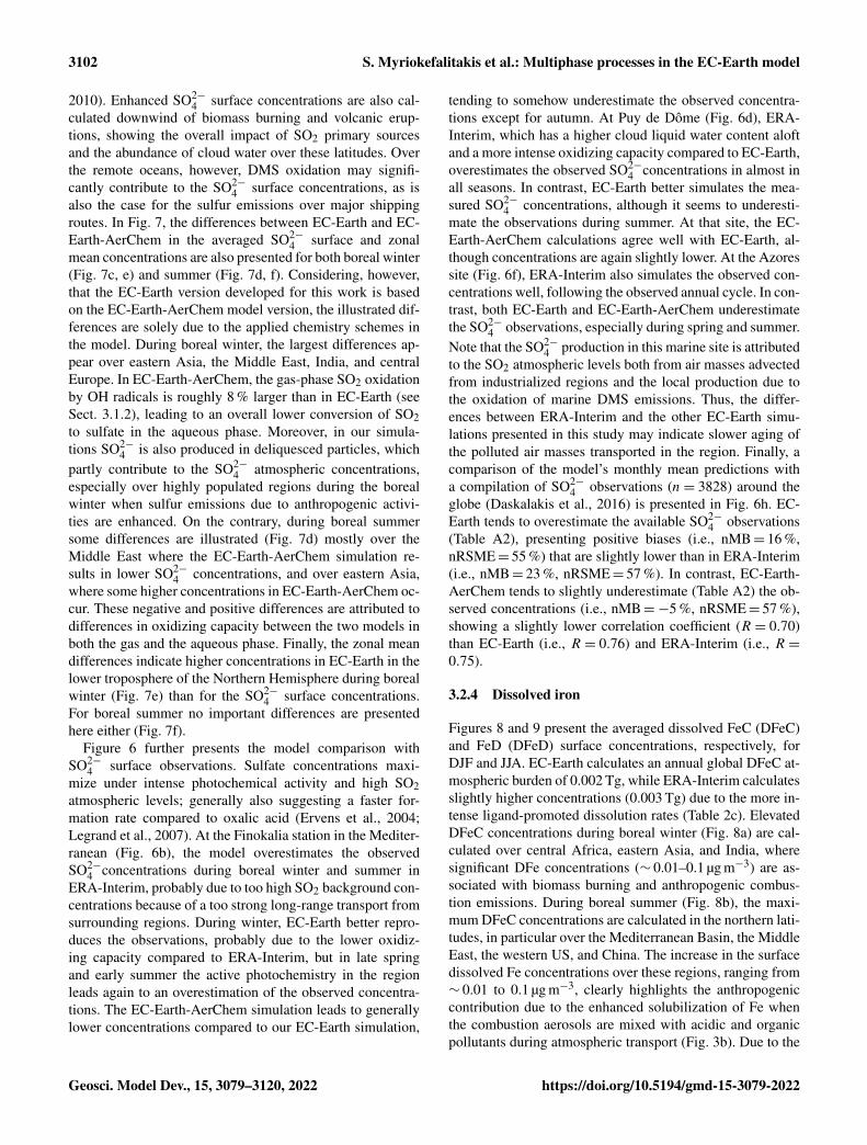
3102 S. Myriokefalitakis et al.: Multiphase processes in the EC-Earth model
2010). Enhanced SO2−4 surface concentrations are also cal-
culated downwind of biomass burning and volcanic erup-tions, showing the overall impact of SO2 primary sourcesand the abundance of cloud water over these latitudes. Overthe remote oceans, however, DMS oxidation may signifi-cantly contribute to the SO2−
4 surface concentrations, as isalso the case for the sulfur emissions over major shippingroutes. In Fig. 7, the differences between EC-Earth and EC-Earth-AerChem in the averaged SO2−
4 surface and zonalmean concentrations are also presented for both boreal winter(Fig. 7c, e) and summer (Fig. 7d, f). Considering, however,that the EC-Earth version developed for this work is basedon the EC-Earth-AerChem model version, the illustrated dif-ferences are solely due to the applied chemistry schemes inthe model. During boreal winter, the largest differences ap-pear over eastern Asia, the Middle East, India, and centralEurope. In EC-Earth-AerChem, the gas-phase SO2 oxidationby OH radicals is roughly 8 % larger than in EC-Earth (seeSect. 3.1.2), leading to an overall lower conversion of SO2to sulfate in the aqueous phase. Moreover, in our simula-tions SO2−
4 is also produced in deliquesced particles, whichpartly contribute to the SO2−
4 atmospheric concentrations,especially over highly populated regions during the borealwinter when sulfur emissions due to anthropogenic activi-ties are enhanced. On the contrary, during boreal summersome differences are illustrated (Fig. 7d) mostly over theMiddle East where the EC-Earth-AerChem simulation re-sults in lower SO2−
4 concentrations, and over eastern Asia,where some higher concentrations in EC-Earth-AerChem oc-cur. These negative and positive differences are attributed todifferences in oxidizing capacity between the two models inboth the gas and the aqueous phase. Finally, the zonal meandifferences indicate higher concentrations in EC-Earth in thelower troposphere of the Northern Hemisphere during borealwinter (Fig. 7e) than for the SO2−
4 surface concentrations.For boreal summer no important differences are presentedhere either (Fig. 7f).
Figure 6 further presents the model comparison withSO2−
4 surface observations. Sulfate concentrations maxi-mize under intense photochemical activity and high SO2atmospheric levels; generally also suggesting a faster for-mation rate compared to oxalic acid (Ervens et al., 2004;Legrand et al., 2007). At the Finokalia station in the Mediter-ranean (Fig. 6b), the model overestimates the observedSO2−
4 concentrations during boreal winter and summer inERA-Interim, probably due to too high SO2 background con-centrations because of a too strong long-range transport fromsurrounding regions. During winter, EC-Earth better repro-duces the observations, probably due to the lower oxidiz-ing capacity compared to ERA-Interim, but in late springand early summer the active photochemistry in the regionleads again to an overestimation of the observed concentra-tions. The EC-Earth-AerChem simulation leads to generallylower concentrations compared to our EC-Earth simulation,
tending to somehow underestimate the observed concentra-tions except for autumn. At Puy de Dôme (Fig. 6d), ERA-Interim, which has a higher cloud liquid water content aloftand a more intense oxidizing capacity compared to EC-Earth,overestimates the observed SO2−
4 concentrations in almost inall seasons. In contrast, EC-Earth better simulates the mea-sured SO2−
4 concentrations, although it seems to underesti-mate the observations during summer. At that site, the EC-Earth-AerChem calculations agree well with EC-Earth, al-though concentrations are again slightly lower. At the Azoressite (Fig. 6f), ERA-Interim also simulates the observed con-centrations well, following the observed annual cycle. In con-trast, both EC-Earth and EC-Earth-AerChem underestimatethe SO2−
4 observations, especially during spring and summer.Note that the SO2−
4 production in this marine site is attributedto the SO2 atmospheric levels both from air masses advectedfrom industrialized regions and the local production due tothe oxidation of marine DMS emissions. Thus, the differ-ences between ERA-Interim and the other EC-Earth simu-lations presented in this study may indicate slower aging ofthe polluted air masses transported in the region. Finally, acomparison of the model’s monthly mean predictions witha compilation of SO2−
4 observations (n= 3828) around theglobe (Daskalakis et al., 2016) is presented in Fig. 6h. EC-Earth tends to overestimate the available SO2−
4 observations(Table A2), presenting positive biases (i.e., nMB= 16 %,nRSME= 55 %) that are slightly lower than in ERA-Interim(i.e., nMB= 23 %, nRSME= 57 %). In contrast, EC-Earth-AerChem tends to slightly underestimate (Table A2) the ob-served concentrations (i.e., nMB=−5 %, nRSME= 57 %),showing a slightly lower correlation coefficient (R = 0.70)than EC-Earth (i.e., R = 0.76) and ERA-Interim (i.e., R =0.75).
3.2.4 Dissolved iron
Figures 8 and 9 present the averaged dissolved FeC (DFeC)and FeD (DFeD) surface concentrations, respectively, forDJF and JJA. EC-Earth calculates an annual global DFeC at-mospheric burden of 0.002 Tg, while ERA-Interim calculatesslightly higher concentrations (0.003 Tg) due to the more in-tense ligand-promoted dissolution rates (Table 2c). ElevatedDFeC concentrations during boreal winter (Fig. 8a) are cal-culated over central Africa, eastern Asia, and India, wheresignificant DFe concentrations (∼ 0.01–0.1 µg m−3) are as-sociated with biomass burning and anthropogenic combus-tion emissions. During boreal summer (Fig. 8b), the maxi-mum DFeC concentrations are calculated in the northern lati-tudes, in particular over the Mediterranean Basin, the MiddleEast, the western US, and China. The increase in the surfacedissolved Fe concentrations over these regions, ranging from∼ 0.01 to 0.1 µg m−3, clearly highlights the anthropogeniccontribution due to the enhanced solubilization of Fe whenthe combustion aerosols are mixed with acidic and organicpollutants during atmospheric transport (Fig. 3b). Due to the
Geosci. Model Dev., 15, 3079–3120, 2022 https://doi.org/10.5194/gmd-15-3079-2022
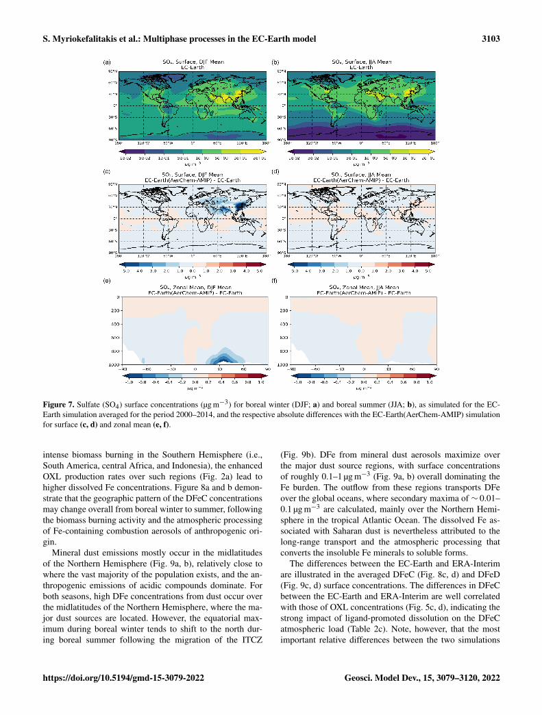
S. Myriokefalitakis et al.: Multiphase processes in the EC-Earth model 3103
Figure 7. Sulfate (SO4) surface concentrations (µg m−3) for boreal winter (DJF; a) and boreal summer (JJA; b), as simulated for the EC-Earth simulation averaged for the period 2000–2014, and the respective absolute differences with the EC-Earth(AerChem-AMIP) simulationfor surface (c, d) and zonal mean (e, f).
intense biomass burning in the Southern Hemisphere (i.e.,South America, central Africa, and Indonesia), the enhancedOXL production rates over such regions (Fig. 2a) lead tohigher dissolved Fe concentrations. Figure 8a and b demon-strate that the geographic pattern of the DFeC concentrationsmay change overall from boreal winter to summer, followingthe biomass burning activity and the atmospheric processingof Fe-containing combustion aerosols of anthropogenic ori-gin.
Mineral dust emissions mostly occur in the midlatitudesof the Northern Hemisphere (Fig. 9a, b), relatively close towhere the vast majority of the population exists, and the an-thropogenic emissions of acidic compounds dominate. Forboth seasons, high DFe concentrations from dust occur overthe midlatitudes of the Northern Hemisphere, where the ma-jor dust sources are located. However, the equatorial max-imum during boreal winter tends to shift to the north dur-ing boreal summer following the migration of the ITCZ
(Fig. 9b). DFe from mineral dust aerosols maximize overthe major dust source regions, with surface concentrationsof roughly 0.1–1 µg m−3 (Fig. 9a, b) overall dominating theFe burden. The outflow from these regions transports DFeover the global oceans, where secondary maxima of ∼ 0.01–0.1 µg m−3 are calculated, mainly over the Northern Hemi-sphere in the tropical Atlantic Ocean. The dissolved Fe as-sociated with Saharan dust is nevertheless attributed to thelong-range transport and the atmospheric processing thatconverts the insoluble Fe minerals to soluble forms.
The differences between the EC-Earth and ERA-Interimare illustrated in the averaged DFeC (Fig. 8c, d) and DFeD(Fig. 9c, d) surface concentrations. The differences in DFeCbetween the EC-Earth and ERA-Interim are well correlatedwith those of OXL concentrations (Fig. 5c, d), indicating thestrong impact of ligand-promoted dissolution on the DFeCatmospheric load (Table 2c). Note, however, that the mostimportant relative differences between the two simulations
https://doi.org/10.5194/gmd-15-3079-2022 Geosci. Model Dev., 15, 3079–3120, 2022
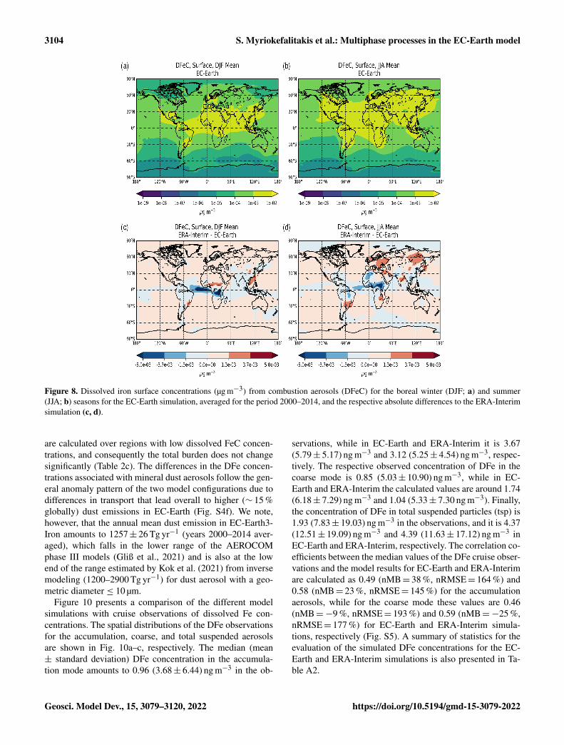
3104 S. Myriokefalitakis et al.: Multiphase processes in the EC-Earth model
Figure 8. Dissolved iron surface concentrations (µg m−3) from combustion aerosols (DFeC) for the boreal winter (DJF; a) and summer(JJA; b) seasons for the EC-Earth simulation, averaged for the period 2000–2014, and the respective absolute differences to the ERA-Interimsimulation (c, d).
are calculated over regions with low dissolved FeC concen-trations, and consequently the total burden does not changesignificantly (Table 2c). The differences in the DFe concen-trations associated with mineral dust aerosols follow the gen-eral anomaly pattern of the two model configurations due todifferences in transport that lead overall to higher (∼ 15 %globally) dust emissions in EC-Earth (Fig. S4f). We note,however, that the annual mean dust emission in EC-Earth3-Iron amounts to 1257± 26 Tg yr−1 (years 2000–2014 aver-aged), which falls in the lower range of the AEROCOMphase III models (Gliß et al., 2021) and is also at the lowend of the range estimated by Kok et al. (2021) from inversemodeling (1200–2900 Tg yr−1) for dust aerosol with a geo-metric diameter ≤ 10 µm.
Figure 10 presents a comparison of the different modelsimulations with cruise observations of dissolved Fe con-centrations. The spatial distributions of the DFe observationsfor the accumulation, coarse, and total suspended aerosolsare shown in Fig. 10a–c, respectively. The median (mean± standard deviation) DFe concentration in the accumula-tion mode amounts to 0.96 (3.68± 6.44) ng m−3 in the ob-
servations, while in EC-Earth and ERA-Interim it is 3.67(5.79± 5.17) ng m−3 and 3.12 (5.25± 4.54) ng m−3, respec-tively. The respective observed concentration of DFe in thecoarse mode is 0.85 (5.03± 10.90) ng m−3, while in EC-Earth and ERA-Interim the calculated values are around 1.74(6.18± 7.29) ng m−3 and 1.04 (5.33± 7.30 ng m−3). Finally,the concentration of DFe in total suspended particles (tsp) is1.93 (7.83± 19.03) ng m−3 in the observations, and it is 4.37(12.51± 19.09) ng m−3 and 4.39 (11.63± 17.12) ng m−3 inEC-Earth and ERA-Interim, respectively. The correlation co-efficients between the median values of the DFe cruise obser-vations and the model results for EC-Earth and ERA-Interimare calculated as 0.49 (nMB= 38 %, nRMSE= 164 %) and0.58 (nMB= 23 %, nRMSE= 145 %) for the accumulationaerosols, while for the coarse mode these values are 0.46(nMB=−9 %, nRMSE= 193 %) and 0.59 (nMB=−25 %,nRMSE= 177 %) for EC-Earth and ERA-Interim simula-tions, respectively (Fig. S5). A summary of statistics for theevaluation of the simulated DFe concentrations for the EC-Earth and ERA-Interim simulations is also presented in Ta-ble A2.
Geosci. Model Dev., 15, 3079–3120, 2022 https://doi.org/10.5194/gmd-15-3079-2022
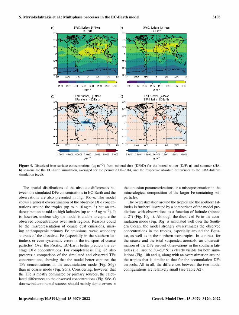
S. Myriokefalitakis et al.: Multiphase processes in the EC-Earth model 3105
Figure 9. Dissolved iron surface concentrations (µg m−3) from mineral dust (DFeD) for the boreal winter (DJF; a) and summer (JJA;b) seasons for the EC-Earth simulation, averaged for the period 2000–2014, and the respective absolute differences to the ERA-Interimsimulation (c, d).
The spatial distributions of the absolute differences be-tween the simulated DFe concentrations in EC-Earth and theobservations are also presented in Fig. 10d–e. The modelshows a general overestimation of the observed DFe concen-trations around the tropics (up to ∼ 10 ng m−3) but an un-derestimation at mid-to-high latitudes (up to ∼ 5 ng m−3). Itis, however, unclear why the model is unable to capture theobserved concentrations over such regions. Reasons couldbe the misrepresentation of coarse dust emissions, miss-ing anthropogenic primary Fe emissions, weak secondarysources of the dissolved Fe (especially in the southern lat-itudes), or even systematic errors in the transport of coarseparticles. Over the Pacific, EC-Earth better predicts the av-erage DFe concentrations. For completeness, Fig. S5 alsopresents a comparison of the simulated and observed TFeconcentrations, showing that the model better captures theTFe concentrations in the accumulation mode (Fig. S6g)than in coarse mode (Fig. S6h). Considering, however, thatthe TFe is mostly dominated by primary sources, the calcu-lated differences to the observed concentrations (Fig. S6e–f)downwind continental sources should mainly depict errors in
the emission parameterizations or a misrepresentation in themineralogical composition of the larger Fe-containing soilparticles.
The overestimation around the tropics and the northern lat-itudes is further illustrated by a comparison of the model pre-dictions with observations as a function of latitude (binnedat 2◦) (Fig. 10g–i). Although the dissolved Fe in the accu-mulation mode (Fig. 10g) is simulated well over the South-ern Ocean, the model strongly overestimates the observedconcentrations in the tropics, especially around the Equa-tor, as well as in the northern extratropics. In contrast, forthe coarse and the total suspended aerosols, an underesti-mation of the DFe aerosol observations in the southern lati-tudes (i.e., around 30–60◦ S) is clearly visible for both simu-lations (Fig. 10h and i), along with an overestimation aroundthe tropics that is similar to that for the accumulation DFeaerosols. All in all, the differences between the two modelconfigurations are relatively small (see Table A2).
https://doi.org/10.5194/gmd-15-3079-2022 Geosci. Model Dev., 15, 3079–3120, 2022
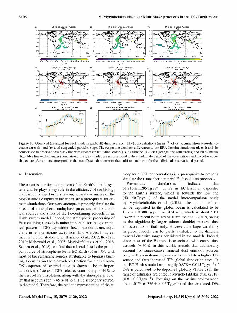
3106 S. Myriokefalitakis et al.: Multiphase processes in the EC-Earth model
Figure 10. Observed (averaged for each model’s grid-cell) dissolved iron (DFe) concentrations (ng m−3) of (a) accumulation aerosols, (b)coarse aerosols, and (c) total suspended particles (tsp). The respective absolute differences to the ERA-Interim simulation (d, e, f) and thecomparison to observations (black line with crosses) in latitudinal order (g, e, f) with the EC-Earth (orange line with circles) and ERA-Interim(light blue line with triangles) simulations; the grey-shaded areas correspond to the standard deviation of the observations and the color-codedshaded areas/error bars correspond to the model’s standard error of the multi-annual mean for the individual observational period.
4 Discussion
The ocean is a critical component of the Earth’s climate sys-tem, and Fe plays a key role in the efficiency of the biolog-ical carbon pump. For this reason, accurate estimates of thebioavailable Fe inputs to the ocean are a prerequisite for cli-mate simulations. Our work attempts to properly simulate theeffects of atmospheric multiphase processes on the chem-ical sources and sinks of the Fe-containing aerosols in anEarth system model. Indeed, the atmospheric processing ofFe-containing aerosols is rather important for the geograph-ical pattern of DFe deposition fluxes into the ocean, espe-cially in remote regions away from land sources. In agree-ment with other studies (e.g., Hamilton et al., 2022; Ito et al.,2019; Mahowald et al., 2005; Myriokefalitakis et al., 2018;Scanza et al., 2018), we find that mineral dust is the princi-pal source of atmospheric Fe in EC-Earth (95± 1 %), withmost of the remaining sources attributable to biomass burn-ing. Focusing on the bioavailable fraction for marine biota,OXL aqueous-phase production is shown to be an impor-tant driver of aerosol DFe release, contributing ∼ 44 % tothe aerosol Fe dissolution, along with the atmospheric acid-ity that accounts for ∼ 45 % of total DFe secondary sourcesin the model. Therefore, the realistic representation of the at-
mospheric OXL concentrations is a prerequisite to properlysimulate the atmospheric mineral Fe dissolution processes.
Present-day simulations indicate that61.816± 1.295 Tg yr−1 of Fe in EC-Earth is depositedto the Earth’s surface, which is towards the low end(40–140 Tg yr−1) of the model intercomparison studyby Myriokefalitakis et al. (2018). The amount of to-tal Fe deposited to the global ocean is calculated to be12.937± 0.308 Tg yr−1 in EC-Earth, which is about 50 %lower than recent estimates by Hamilton et al. (2019), owingto the significantly larger (almost double) mineral dustemission flux in that study. However, the large variabilityin global models can be partly attributed to the differentmineral dust size ranges considered in the models. Indeed,since most of the Fe mass is associated with coarse dustaerosols (∼ 91 % in this work), models that additionallyaccount for super-coarse mineral dust emission sources(i.e., >10 µm in diameter) eventually calculate a higher TFesource and thus increased TFe global deposition rates. Inour EC-Earth simulations, roughly 0.878± 0.015 Tg yr−1 ofDFe is calculated to be deposited globally (Table 2) in therange of estimates presented in Myriokefalitakis et al. (2018)(0.8± 0.2 Tg yr−1). Focusing on the marine environment,about 40 % (0.376± 0.005 Tg yr−1) of the simulated DFe
Geosci. Model Dev., 15, 3079–3120, 2022 https://doi.org/10.5194/gmd-15-3079-2022

S. Myriokefalitakis et al.: Multiphase processes in the EC-Earth model 3107
Figure 11. Annual mean Fe-containing aerosol solubility at depo-sition fluxes (%) as simulated for the EC-Earth simulation averagedfor the period 2000–2014 for (a) mineral dust aerosols; (b) the sumof solid fuel combustion, liquid fuel combustion, and open biomassburning aerosols; and (c) the sum of all aerosol sources.
is deposited into the global ocean, indicating that a largefraction of Fe atmospheric inputs to the global ocean resultsfrom the dissolution of atmospheric aerosols. Our resultsare close to the high-end of other global estimates (0.173–0.419 Tg yr−1) as presented in the model intercomparison
study of Myriokefalitakis et al. (2018), slightly higher thanthe respective DFe deposition fluxes in Ito et al. (2021)(0.271 Tg yr−1) but somehow lower compared to Hamiltonet al. (2019) estimates (roughly 0.5 Tg yr−1), although thesignificant differences in the dust emission fluxes. Thus,even though we do not consider a super-coarse mode ofdust in our simulations, the DFe deposition rates over theremote ocean are not severely impacted (Myriokefalitakiset al., 2018) by the size of the emitted minerals, but insteadby the atmospheric processing during long-range transport.Nevertheless, reaching a firm conclusion in that respect willneed further work.
The Fe-containing dust aerosols dominate (∼ 70 %) the to-tal deposition fluxes over the ocean in the model, althoughcombustion sources are calculated to have a significant im-pact on the Fe inputs to remote oceanic regions, such as thePacific and the Southern Oceans, in agreement with otherstudies (e.g., Hamilton et al., 2020). The maximum DFe de-position fluxes occur in EC-Earth downwind of the maindesert source regions, with high deposition rates being simu-lated in the outflow of tropical biomass burning regions (suchas South America, Africa, and Indonesia), as well as overhighly populated regions due to the Fe released from anthro-pogenic combustion processes in the presence of polluted airmasses (such as in India and China). Overall, the average Fesolubility at the deposition of combustion aerosols is foundhere ∼ 19 % (Fig. 11a), much higher compared to the sol-ubility of mineral dust aerosols (∼ 2 %; Fig. 11b), clearlyindicating the importance of atmospheric processing on thepotential bioavailable inputs to the global ocean. We furthernote that although a relatively high Fe solubility is appliedhere for oil fly ash emission (∼ 79 %), a sensitivity simula-tion (not shown) using a solubility for ship oil emissions of47.5 %, as proposed by Rathod et al. (2020), leads to overallan only slight decrease (up to ∼ 2 %) in Fe solubility calcu-lations, mainly in the northern Atlantic Ocean, and does notsubstantially affect our results. Indeed, our simulations showhigh Fe solubilities far from continental regions (Fig. S6g–i),such as the tropical Pacific and Atlantic Oceans (Fig. 11c),due to aerosol aging and lower Fe concentrations. Note thatan evaluation of Fe solubility model calculation over oceanicregions (based on cruise measurements, where available) isalso provided here (Fig. S5), showing overall a general over-estimation of the observed values (Table A2) with neverthe-less both positive and negative biases.
5 Summary and conclusions
This work documents the implementation of a detailed mul-tiphase chemistry scheme in the EC-Earth3 Earth systemmodel, aiming to provide consistent estimates of the atmo-spheric concentrations of the Fe-containing aerosols, alongwith the species that modulates its atmospheric processing,i.e., OXL and SO2−
4 . For this, a comprehensive description of
https://doi.org/10.5194/gmd-15-3079-2022 Geosci. Model Dev., 15, 3079–3120, 2022

3108 S. Myriokefalitakis et al.: Multiphase processes in the EC-Earth model
the atmospheric Fe cycle is included in the model, account-ing for (1) an explicit soil mineralogy, (2) the contributionof combustion emissions, and (3) an atmospheric dissolu-tion scheme that accounts for atmospheric acidity, ambientlevels of OXL, and photoinduced processes. The multiphasechemistry scheme simulates the aqueous-phase processes ofthe troposphere for inorganic and organic compounds, alongwith the Fenton reaction. The KPP software is used in themodel to integrate the aqueous phase and the dissolutionequations, which adds flexibility to the code. Overall, simula-tions of tropospheric chemistry and aerosols for present-dayconditions (2000–2014) have been realized, and budget cal-culations for OXL, SO2−
4 , and the DFe-containing aerosolshave been presented.
Model simulations have been performed both as a cou-pled system with IFS, as well as driven by offline mete-orological fields from the ERA-Interim reanalysis. Budgetanalysis has shown that glyoxal is the main precursor ofOXL in the atmosphere (∼ 74 %) and that the potential pri-mary sources in the model (0.373± 0.005 Tg yr−1) have anegligible impact on OXL concentrations. Non-traditional,laboratory-derived, aqueous-phase production pathways ofOXL via glyoxal oxidation are also accounted for in oursimulations. We have shown that when such pathways areomitted in the simulations, the calculated global OXL atmo-spheric concentrations are substantially lowered (∼ 43 %).For the ERA-Interim setup, the OXL net chemical produc-tion is calculated as 18.116± 0.071 Tg yr−1, resulting in anatmospheric burden of 0.330 Tg on average. For the online-coupled system, however, the OXL net chemical productionis ∼ 30 % lower, mainly attributed to a lower atmosphericOH abundance in EC-Earth due to biases that can be gen-erally found in climate–chemistry models, such as those fortemperature and humidity, especially at the higher altitudes.Overall, the simulated oxidizing capacity, along with the con-tribution of secondary sources other than the GLX oxidation,are shown to have a significant impact on the OXL atmo-spheric abundance. However, we acknowledge that other for-mation pathways of OXL, primary or secondary, may exist inthe gas and aqueous phases of the atmosphere that could fur-ther contribute to OXL levels.
The dissolution of dust and combustion aerosols domi-nates on the dissolved Fe fraction in the model, calculated inEC-Earth at 0.806± 0.014 Tg yr−1, in good agreement withthe ERA-Interim simulation and well in the range of othermodel estimates. Furthermore, a broad evaluation of the EC-Earth proves the models’ ability to represent AOD, par-ticularly over regions that are dominated by anthropogenicaerosol but also over selected dusty sites, in line with previ-ous EC-Earth evaluations. However, dust is underestimatedover most remote areas, implying the EC-Earth shares thedifficulties of many global models in representing the long-range transport of dust, especially the coarse particles. Themodel also underestimates the in situ OXL measurements,especially during winter, nevertheless indicating that addi-
tional sources (primary and/or secondary) are needed. Modelcomparisons with cruise measurements demonstrate a stronglink between atmospheric DFe concentrations and atmo-spheric composition. The model seems to better capture theobservations in the accumulation mode than in the coarsemode. This is attributed to differences either in the atmo-spheric processing between the accumulation and coarse par-ticles (i.e., aerosol water content and acidity levels), the mis-representation in the aerosol sizes (e.g., surface area/volumeratios), or to systematic errors in the mineralogical composi-tion of the emitted Fe-containing soil particles. For this, sev-eral developments are planned by the EC-Earth consortium,aiming to improve the representation of the dust aerosols’size distribution, the description of the mineralogical com-position, and the Fe-content in combustion sources, whichare expected to reduce the existing uncertainties in the modelfor a more accurate simulation of the atmospheric Fe cycle.
Emphasizing on the biogeochemistry-related implicationsof this study, EC-Earth calculates a global annual present-day DFe deposition flux of 0.878± 0.015 Tg yr−1, which iswell within the range of estimates of other global modelingstudies. About 40 % of the DFe deposition fluxes are calcu-lated to occur over the global ocean (0.376± 0.005 Tg yr−1),with a strong spatial and temporal variability. The highestannual mean DFe inputs to the global ocean are associatedwith aerosols of soil origin, especially downwind of the ma-jor dust source regions. In addition, Fe-containing combus-tion aerosols are calculated to have a significant contribu-tion downwind of biomass burning source regions and highlypopulated areas in the Northern Hemisphere. It is furtherdemonstrated that over the open ocean the Fe solubility atdeposition for aerosols of combustion origin is about an or-der of magnitude higher than that of mineral dust origin, sug-gesting that the relative contributions of the primary sourcescan significantly affect bioavailable aerosol fraction and maythus play an important role in oceanic areas where the phyto-plankton growth is limited by Fe supply, such as the SouthernOcean.
It is widely recognized that a combined approach consid-ering both Fe atmospheric processing and deposition overoceans should ideally be used in Earth system models forthe assessment of the impact of nutrient-containing aerosoldeposition on marine productivity. A deeper understandingof the atmospheric Fe cycle is thus needed for a better de-scription of the biogeochemistry implications in the presenceof a changing climate. Such types of knowledge, however,should be obtained by extensive model evaluation with ob-servations, especially over the remote regions of the worldlike the Southern Ocean, where currently the largest discrep-ancies between models and measurements exist. Therefore, acomprehensive calculation of the Fe physicochemical trans-formations is necessary to predict the strength of DFe inputsto the ocean, despite the complexity of the related atmo-spheric multiphase processes. The present study thus aimsto complement the marine biogeochemistry component of
Geosci. Model Dev., 15, 3079–3120, 2022 https://doi.org/10.5194/gmd-15-3079-2022
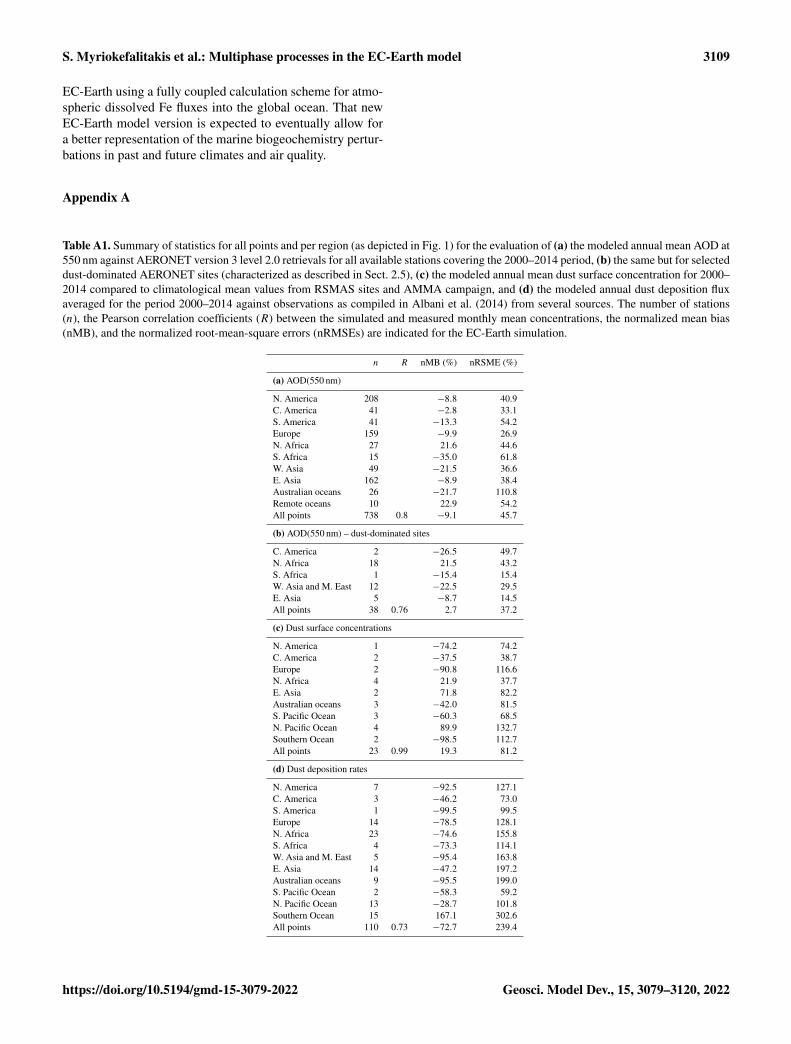
S. Myriokefalitakis et al.: Multiphase processes in the EC-Earth model 3109
EC-Earth using a fully coupled calculation scheme for atmo-spheric dissolved Fe fluxes into the global ocean. That newEC-Earth model version is expected to eventually allow fora better representation of the marine biogeochemistry pertur-bations in past and future climates and air quality.
Appendix A
Table A1. Summary of statistics for all points and per region (as depicted in Fig. 1) for the evaluation of (a) the modeled annual mean AOD at550 nm against AERONET version 3 level 2.0 retrievals for all available stations covering the 2000–2014 period, (b) the same but for selecteddust-dominated AERONET sites (characterized as described in Sect. 2.5), (c) the modeled annual mean dust surface concentration for 2000–2014 compared to climatological mean values from RSMAS sites and AMMA campaign, and (d) the modeled annual dust deposition fluxaveraged for the period 2000–2014 against observations as compiled in Albani et al. (2014) from several sources. The number of stations(n), the Pearson correlation coefficients (R) between the simulated and measured monthly mean concentrations, the normalized mean bias(nMB), and the normalized root-mean-square errors (nRMSEs) are indicated for the EC-Earth simulation.
n R nMB (%) nRSME (%)
(a) AOD(550 nm)
N. America 208 −8.8 40.9C. America 41 −2.8 33.1S. America 41 −13.3 54.2Europe 159 −9.9 26.9N. Africa 27 21.6 44.6S. Africa 15 −35.0 61.8W. Asia 49 −21.5 36.6E. Asia 162 −8.9 38.4Australian oceans 26 −21.7 110.8Remote oceans 10 22.9 54.2All points 738 0.8 −9.1 45.7
(b) AOD(550 nm) – dust-dominated sites
C. America 2 −26.5 49.7N. Africa 18 21.5 43.2S. Africa 1 −15.4 15.4W. Asia and M. East 12 −22.5 29.5E. Asia 5 −8.7 14.5All points 38 0.76 2.7 37.2
(c) Dust surface concentrations
N. America 1 −74.2 74.2C. America 2 −37.5 38.7Europe 2 −90.8 116.6N. Africa 4 21.9 37.7E. Asia 2 71.8 82.2Australian oceans 3 −42.0 81.5S. Pacific Ocean 3 −60.3 68.5N. Pacific Ocean 4 89.9 132.7Southern Ocean 2 −98.5 112.7All points 23 0.99 19.3 81.2
(d) Dust deposition rates
N. America 7 −92.5 127.1C. America 3 −46.2 73.0S. America 1 −99.5 99.5Europe 14 −78.5 128.1N. Africa 23 −74.6 155.8S. Africa 4 −73.3 114.1W. Asia and M. East 5 −95.4 163.8E. Asia 14 −47.2 197.2Australian oceans 9 −95.5 199.0S. Pacific Ocean 2 −58.3 59.2N. Pacific Ocean 13 −28.7 101.8Southern Ocean 15 167.1 302.6All points 110 0.73 −72.7 239.4
https://doi.org/10.5194/gmd-15-3079-2022 Geosci. Model Dev., 15, 3079–3120, 2022
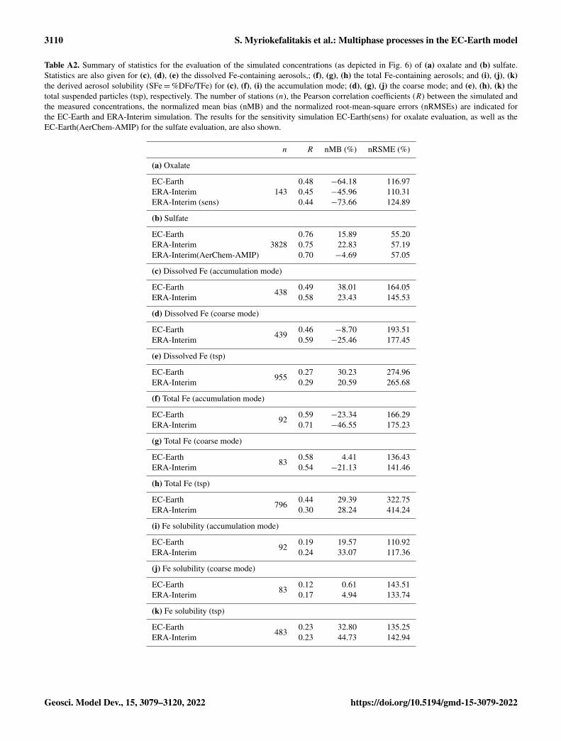
3110 S. Myriokefalitakis et al.: Multiphase processes in the EC-Earth model
Table A2. Summary of statistics for the evaluation of the simulated concentrations (as depicted in Fig. 6) of (a) oxalate and (b) sulfate.Statistics are also given for (c), (d), (e) the dissolved Fe-containing aerosols,; (f), (g), (h) the total Fe-containing aerosols; and (i), (j), (k)the derived aerosol solubility (SFe=%DFe/TFe) for (c), (f), (i) the accumulation mode; (d), (g), (j) the coarse mode; and (e), (h), (k) thetotal suspended particles (tsp), respectively. The number of stations (n), the Pearson correlation coefficients (R) between the simulated andthe measured concentrations, the normalized mean bias (nMB) and the normalized root-mean-square errors (nRMSEs) are indicated forthe EC-Earth and ERA-Interim simulation. The results for the sensitivity simulation EC-Earth(sens) for oxalate evaluation, as well as theEC-Earth(AerChem-AMIP) for the sulfate evaluation, are also shown.
n R nMB (%) nRSME (%)
(a) Oxalate
EC-Earth 0.48 −64.18 116.97ERA-Interim 143 0.45 −45.96 110.31ERA-Interim (sens) 0.44 −73.66 124.89
(b) Sulfate
EC-Earth 0.76 15.89 55.20ERA-Interim 3828 0.75 22.83 57.19ERA-Interim(AerChem-AMIP) 0.70 −4.69 57.05
(c) Dissolved Fe (accumulation mode)
EC-Earth438
0.49 38.01 164.05ERA-Interim 0.58 23.43 145.53
(d) Dissolved Fe (coarse mode)
EC-Earth439
0.46 −8.70 193.51ERA-Interim 0.59 −25.46 177.45
(e) Dissolved Fe (tsp)
EC-Earth955
0.27 30.23 274.96ERA-Interim 0.29 20.59 265.68
(f) Total Fe (accumulation mode)
EC-Earth92
0.59 −23.34 166.29ERA-Interim 0.71 −46.55 175.23
(g) Total Fe (coarse mode)
EC-Earth83
0.58 4.41 136.43ERA-Interim 0.54 −21.13 141.46
(h) Total Fe (tsp)
EC-Earth796
0.44 29.39 322.75ERA-Interim 0.30 28.24 414.24
(i) Fe solubility (accumulation mode)
EC-Earth92
0.19 19.57 110.92ERA-Interim 0.24 33.07 117.36
(j) Fe solubility (coarse mode)
EC-Earth83
0.12 0.61 143.51ERA-Interim 0.17 4.94 133.74
(k) Fe solubility (tsp)
EC-Earth483
0.23 32.80 135.25ERA-Interim 0.23 44.73 142.94
Geosci. Model Dev., 15, 3079–3120, 2022 https://doi.org/10.5194/gmd-15-3079-2022
S. Myriokefalitakis et al.: Multiphase processes in the EC-Earth model 3111
Code availability. The EC-Earth3-Iron code is available from theEC-Earth development portal (https://dev.ec-earth.org/, last access:3 December 2021) for members of the consortium. EC-Earth3-Ironadds new features to the EC-Earth-AerChem version 3.3.2.1, whichincludes the IFS cycle 36r4, the NEMO-LIM3 release 3.6, and theTM5-MP 3.0 and makes use of the OASIS3-MCT version 3.0 cou-pler. An AMIP reader is also available to use ocean prescribeddata. Model codes developed at ECMWF, including the atmospheremodel IFS, are intellectual property of ECMWF and its memberstates. Permission to access the EC-Earth3-Iron source code canbe requested from the EC-Earth community via the EC-Earth web-site (http://www.ec-earth.org/, last access: 26 July 2021) and maybe granted if a corresponding software license agreement is signedwith ECMWF. The corresponding repository tag is 3.3.2.1-Fe. Cur-rently, only European users can be granted access due to licenselimitations of the model.
Data availability. The Aerosol Robotic Network retrievalsof optical depth were downloaded through the AERONETdata download tool (available at: https://aeronet.gsfc.nasa.gov/,NASA, 2020 last access: 28 March 2020). The derived cli-matologies used for model evaluation in Fig. 4 have beenpermanently stored in the Zenodo repository, accessible throughhttps://doi.org/10.5281/zenodo.5776347 (Gonçalves Ageitoset al., 2021). Access to the observations of dust concentra-tion from the AMMA campaign can be requested throughthe INDAAF website (https://indaaf.obs-mip.fr/, Marticorena,2021). Other observational datasets used for evaluation areavailable in the referenced articles. ERA-Interim data areavailable through the ECMWF data download site (https://apps.ecmwf.int/datasets/data/interim-full-daily/levtype=sfc/,Dee et al., 2011), and the gridded emission and forc-ing datasets, as well as ocean surface conditions used inthis work, are available through the input4MIPs down-load tool (https://esgf-node.llnl.gov/projects/input4mips/,last access: 2 December 2019; for emissions and forc-ings: https://doi.org/10.22033/ESGF/input4MIPs.1604,Hoesly et al., 2017; and for sea ice and SST:https://doi.org/10.22033/ESGF/input4MIPs.1735, Durack etal. 2017). The model outputs relevant for this study are per-manently stored in the Zenodo repository, accessible throughhttps://doi.org/10.5281/zenodo.5752596 (Myriokefalitakis et al.,2021).
Supplement. The supplement related to this article is available on-line at: https://doi.org/10.5194/gmd-15-3079-2022-supplement.
Author contributions. SM developed the aqueous-phase chemistryand the iron-dissolution schemes, designed the experiments, andperformed the ERA-Interim simulations. EBM, MGA, and CPGPdeveloped the mineralogy applied to dust emissions, co-designedthe experiments, and performed the EC-Earth simulations. AI pro-vided the Fe-containing combustion aerosol emissions. EA con-tributed to the emission parameterizations. AN provided the ISOR-ROPIA II code. TVN, PLS, MK, MCK, and EG contributed to thedevelopment of specific aspects of the model or parts of the code
that are shared with the EC-Earth3 community. SM wrote the pa-per, with the contribution of MGA and input from all co-authors.
Competing interests. The contact author has declared that neitherthey nor their co-authors have any competing interests.
Disclaimer. Publisher’s note: Copernicus Publications remainsneutral with regard to jurisdictional claims in published maps andinstitutional affiliations.
Acknowledgements. Stelios Myriokefalitakis, Evangelos Gera-sopoulos, and Maria Kanakidou acknowledge support by the project“PANhellenic infrastructure for Atmospheric Composition and cli-matE change” (MIS 5021516) implemented under the Action“Reinforcement of the Research and Innovation Infrastructure”,which is funded by the Operational Programme “Competitive-ness, Entrepreneurship and Innovation” (NSRF 2014–2020) and co-financed by Greece and the European Union (European RegionalDevelopment Fund). This work was supported by computationaltime granted from the National Infrastructures for Research andTechnology S.A. (GRNET S.A.) in the National HPC facility –ARIS – under project ID 010003 (ANION). Elisa Bergas-Massó,María Gonçalves-Ageitos, and Carlos Pérez García-Pando grate-fully acknowledge the computer resources at Marenostrum4 grantedthrough the PRACE project eFRAGMENT3 and the RES projectAECT-2020-3-0020, as well as the technical support provided bythe Barcelona Supercomputing Center (BSC) and the CES teamof the Earth Sciences Department. Their work was supported bythe ERC Consolidator Grant FRAGMENT (grant agreement no.773051) and the AXA Chair on Sand and Dust Storms at BSCfunded by the AXA Research Fund, both of which are led byCarlos Pérez García-Pando, who also acknowledges the Ramon yCajal program (grant no. RYC-2015-18690) of the Spanish Min-istry of Science, Innovation and Universities and the ICREA pro-gram. The research leading to these results has also received fund-ing from the Spanish Ministerio de Economía y Competitividad aspart of the NUTRIENT project (CGL2017-88911-R) and the H2020GA 821205 project FORCeS. Support for this research was pro-vided to Akinori Ito by the JSPS KAKENHI (grant no. 20H04329)and the Integrated Research Program for Advancing Climate Mod-els (TOUGOU) (grant no. JPMXD0717935715) from the Ministryof Education, Culture, Sports, Science and Technology (MEXT),Japan. Twan van Noije, Philippe Le Sager, Maria Kanakidou, andStelios Myriokefalitakis acknowledge funding from the EuropeanUnion’s 2020 Research And Innovation Programme under grantagreement no. 821205 (FORCeS). Maria Kanakidou acknowledgessupport by the Deutsche Forschungsgemeinschaft (DFG, GermanResearch Foundation) under Germany’s Excellence Strategy (Uni-versity Allowance, EXC 2077, University of Bremen). MaartenC. Krol is supported by the European Research Council (ERC) un-der the European Union’s Horizon 2020 research and innovationprogram under grant agreement no. 742798 (COS-OCS). The au-thors gratefully acknowledge the AERONET and RSMAS PI(s) andtheir staff for establishing and maintaining the sites and data usedin this investigation. PM10 measurements in Banizoumbou (Niger),Cinzana (Mali), an M’Bour (Senegal) were performed in the frame-
https://doi.org/10.5194/gmd-15-3079-2022 Geosci. Model Dev., 15, 3079–3120, 2022

3112 S. Myriokefalitakis et al.: Multiphase processes in the EC-Earth model
work of the French National Observatory Service INDAAF (Inter-national Network to study Deposition and Atmospheric composi-tion in Africa; https://indaaf.obs-mip.fr/, last access: 1 May 2021)piloted by LISA and LAERO and supported by the INSU/CNRS,the IRD, the Observatoire Midi-Pyrénées, the Observatoire des Sci-ences de l’Univers EFLUVE. Model development was carried outon the GRNET HPC ARIS high-performance computer facility, andmodel simulations were performed at the GRNET HPC ARIS andthe BSC Marenostrum4 supercomputer. The authors thank DouglasS. Hamilton and one anonymous reviewer for their comments thatsignificantly helped us to improve the final version of this paper.
Financial support. The publication of this work was financed bythe “PANhellenic infrastructure for Atmospheric Composition andclimatE change” project (grant no. MIS 5021516) co-financed byGreece and the European Union (European Regional DevelopmentFund).
Review statement. This paper was edited by Samuel Remy and re-viewed by Douglas Hamilton and one anonymous referee.
References
Aan de Brugh, J. M. J., Schaap, M., Vignati, E., Dentener, F., Kah-nert, M., Sofiev, M., Huijnen, V., and Krol, M. C.: The Europeanaerosol budget in 2006, Atmos. Chem. Phys., 11, 1117–1139,https://doi.org/10.5194/acp-11-1117-2011, 2011.
Adebiyi, A. A. and Kok, J. F.: Climate models miss most ofthe coarse dust in the atmosphere, Sci. Adv., 6, eaaz9507,https://doi.org/10.1126/sciadv.aaz9507, 2020.
Albani, S., Mahowald, N. M., Perry, A. T., Scanza, R. A., Zen-der, C. S., Heavens, N. G., Maggi, V., Kok, J. F., and Otto-Bliesner, B. L.: Improved dust representation in the Commu-nity Atmosphere Model, J. Adv. Model. Earth Syst., 6, 541–570,https://doi.org/10.1002/2013MS000279, 2014.
Alexander, B., Park, R. J., Jacob, D. J., and Gong, S.: Transitionmetal-catalyzed oxidation of atmospheric sulfur: Global impli-cations for the sulfur budget, J. Geophys. Res., 114, D02309,https://doi.org/10.1029/2008JD010486, 2009.
Altieri, K. E., Carlton, A. G., Lim, H.-J., Turpin, B. J., andSeitzinger, S. P.: Evidence for Oligomer Formation in Clouds:Reactions of Isoprene Oxidation Products, Environ. Sci. Tech-nol., 40, 4956–4960, https://doi.org/10.1021/es052170n, 2006.
Altieri, K. E., Seitzinger, S. P., Carlton, A. G., Turpin, B. J.,Klein, G. C., and Marshall, A. G.: Oligomers formed throughin-cloud methylglyoxal reactions: Chemical composition, prop-erties, and mechanisms investigated by ultra-high resolutionFT-ICR mass spectrometry, Atmos. Environ., 42, 1476–1490,https://doi.org/10.1016/j.atmosenv.2007.11.015, 2008.
Alvarado, L. M. A., Richter, A., Vrekoussis, M., Hilboll, A., KaliszHedegaard, A. B., Schneising, O., and Burrows, J. P.: Unex-pected long-range transport of glyoxal and formaldehyde ob-served from the Copernicus Sentinel-5 Precursor satellite dur-ing the 2018 Canadian wildfires, Atmos. Chem. Phys., 20, 2057–2072, https://doi.org/10.5194/acp-20-2057-2020, 2020.
Arimoto, R., Duce, R. A., Ray, B. J., Ellis, W. G., Cullen, J.D., and Merrill, J. T.: Trace elements in the atmosphere overthe North Atlantic, J. Geophys. Res.-Atmos., 100, 1199–1213,https://doi.org/10.1029/94JD02618, 1995.
Athanasopoulou, E., Tombrou, M., Pandis, S. N., and Russell, A.G.: The role of sea-salt emissions and heterogeneous chemistryin the air quality of polluted coastal areas, Atmos. Chem. Phys.,8, 5755–5769, https://doi.org/10.5194/acp-8-5755-2008, 2008.
Athanasopoulou, E., Protonotariou, A., Papangelis, G., Tombrou,M., Mihalopoulos, N., and Gerasopoulos, E.: Long-rangetransport of Saharan dust and chemical transformations overthe Eastern Mediterranean, Atmos. Environ., 140, 592–604,https://doi.org/10.1016/j.atmosenv.2016.06.041, 2016.
Aumont, O., Ethé, C., Tagliabue, A., Bopp, L., and Gehlen,M.: PISCES-v2: an ocean biogeochemical model for carbonand ecosystem studies, Geosci. Model Dev., 8, 2465–2513,https://doi.org/10.5194/gmd-8-2465-2015, 2015.
Baboukas, E. D., Kanakidou, M., and Mihalopoulos, N.: Car-boxylic acids in gas and particulate phase above the At-lantic Ocean, J. Geophys. Res.-Atmos., 105, 14459–14471,https://doi.org/10.1029/1999JD900977, 2000.
Baker, A. R. and Jickells, T. D.: Atmospheric depositionof soluble trace elements along the Atlantic Merid-ional Transect (AMT), Prog. Oceanogr., 158, 41–51,https://doi.org/10.1016/j.pocean.2016.10.002, 2017.
Balsamo, G., Viterbo, P., Beijaars, A., van den Hurk, B., Hirschi,M., Betts, A. K., and Scipal, K.: A revised hydrology for theECMWF model: Verification from field site to terrestrial waterstorage and impact in the integrated forecast system, J. Hydrom-eteorol., 10, 623–643, https://doi.org/10.1175/2008JHM1068.1,2009.
Bianco, A., Passananti, M., Brigante, M., and Mailhot, G.: Photo-chemistry of the Cloud Aqueous Phase: A Review, Molecules,25, 423, https://doi.org/10.3390/molecules25020423, 2020.
Bibi, I., Singh, B., and Silvester, E.: Dissolution kineticsof soil clays in sulfuric acid solutions: Ionic strengthand temperature effects, Appl. Geochem., 51, 170–183,https://doi.org/10.1016/j.apgeochem.2014.10.004, 2014.
Blando, J. D. and Turpin, B. J.: Secondary organic aerosolformation in cloud and fog droplets: a literature eval-uation of plausibility, Atmos. Environ., 34, 1623–1632,https://doi.org/10.1016/S1352-2310(99)00392-1, 2000.
Bougiatioti, A., Nikolaou, P., Stavroulas, I., Kouvarakis, G., Weber,R., Nenes, A., Kanakidou, M., and Mihalopoulos, N.: Particlewater and pH in the eastern Mediterranean: source variability andimplications for nutrient availability, Atmos. Chem. Phys., 16,4579–4591, https://doi.org/10.5194/acp-16-4579-2016, 2016.
Bowie, A. R., Lannuzel, D., Remenyi, T. A., Wagener, T., Lam,P. J., Boyd, P. W., Guieu, C. C., Townsend, A. T., and Trull, T.W.: Biogeochemical iron budgets of the Southern Ocean southof Australia: Decoupling of iron and nutrient cycles in the sub-antarctic zone by the summertime supply, Global Biogeochem.Cy., 23, GB4034, https://doi.org/10.1029/2009GB003500, 2009.
Bräuer, P., Tilgner, A., Wolke, R., and Herrmann, H.: Mechanismdevelopment and modelling of tropospheric multiphase halo-gen chemistry: The CAPRAM Halogen Module 2.0 (HM2), J.Atmos. Chem., 70, 19–52, https://doi.org/10.1007/s10874-013-9249-6, 2013.
Geosci. Model Dev., 15, 3079–3120, 2022 https://doi.org/10.5194/gmd-15-3079-2022

S. Myriokefalitakis et al.: Multiphase processes in the EC-Earth model 3113
Calvert, J. G., Lazrus, A., Kok, G. L., Heikes, B. G., Walega,J. G., Lind, J., and Cantrell, C. A.: Chemical mechanismsof acid generation in the troposphere, Nature, 317, 27–35,https://doi.org/10.1038/317027a0, 1985.
Cao, F., Zhang, S. C., Kawamura, K., Liu, X., Yang, C., Xu, Z.,Fan, M., Zhang, W., Bao, M., Chang, Y., Song, W., Liu, S., Lee,X., Li, J., Zhang, G., and Zhang, Y. L.: Chemical characteristicsof dicarboxylic acids and related organic compounds in PM2.5during biomass-burning and non-biomass-burning seasons at arural site of Northeast China, Environ. Pollut., 231, 654–662,https://doi.org/10.1016/j.envpol.2017.08.045, 2017.
Cappiello, A., De Simoni, E., Fiorucci, C., Mangani, F., Palma, P.,Trufelli, H., Decesari, S., Facchini, M. C., and Fuzzi, S.: Molecu-lar Characterization of the Water-Soluble Organic Compounds inFogwater by ESIMS/MS, Environ. Sci. Technol., 37, 1229–1240,https://doi.org/10.1021/es0259990, 2003.
Carlton, A. G., Turpin, B. J., Lim, H.-J., Altieri, K. E., andSeitzinger, S.: Link between isoprene and secondary organicaerosol (SOA): Pyruvic acid oxidation yields low volatilityorganic acids in clouds, Geophys. Res. Lett., 33, L06822,https://doi.org/10.1029/2005GL025374, 2006.
Carlton, A. G., Turpin, B. J., Altieri, K. E., Seitzinger, S.,Reff, A., Lim, H.-J., and Ervens, B.: Atmospheric oxalicacid and SOA production from glyoxal: Results of aqueousphotooxidation experiments, Atmos. Environ., 41, 7588–7602,https://doi.org/10.1016/j.atmosenv.2007.05.035, 2007.
Carlton, A. G., Wiedinmyer, C., and Kroll, J. H.: A review of Sec-ondary Organic Aerosol (SOA) formation from isoprene, Atmos.Chem. Phys., 9, 4987–5005, https://doi.org/10.5194/acp-9-4987-2009, 2009.
Chameides, W. L. and Davis, D. D.: Aqueous-phasesource of formic acid in clouds, Nature, 304, 427–429,https://doi.org/10.1038/304427a0, 1983.
Chen, H. and Grassian, V. H.: Iron Dissolution of Dust Source Ma-terials during Simulated Acidic Processing: The Effect of Sulfu-ric, Acetic, and Oxalic Acids, Environ. Sci. Technol., 47, 10312–10321, https://doi.org/10.1021/es401285s, 2013.
Chen, H., Laskin, A., Baltrusaitis, J., Gorski, C. A., Scherer, M.M., and Grassian, V. H.: Coal Fly Ash as a Source of Ironin Atmospheric Dust, Environ. Sci. Technol., 46, 2112–2120,https://doi.org/10.1021/es204102f, 2012.
Christian, T. J., Kleiss, B., Yokelson, R. J., Holzinger, R., Crutzen,P. J., Hao, W. M., Saharjo, B. H., and Ward, D. E.: Comprehen-sive laboratory measurements of biomass-burning emissions: 1.Emissions from Indonesian, African, and other fuels, J. Geophys.Res., 108, 4719, https://doi.org/10.1029/2003JD003704, 2003.
Claquin, T., Schulz, M., and Balkanski, Y. J.: Modeling the mineral-ogy of atmospheric dust sources, J. Geophys. Res.-Atmos., 104,22243–22256, https://doi.org/10.1029/1999JD900416, 1999.
Collett, J. L. J., Hoag, K. J., Rao, X., and Pandis, S. N.: Inter-nal acid buffering in San Joaquin Valley fog drops and its in-fluence on aerosol processing, Atmos. Environ., 33, 4833–4847,https://doi.org/10.1016/S1352-2310(99)00221-6, 1999.
Cong, Z., Kawamura, K., Kang, S., and Fu, P.: Penetration ofbiomass-burning emissions from South Asia through the Hi-malayas: new insights from atmospheric organic acids, Sci. Rep.,5, 9580, https://doi.org/10.1038/srep09580, 2015.
Craig, A., Valcke, S., and Coquart, L.: Development andperformance of a new version of the OASIS coupler,
OASIS3-MCT_3.0, Geosci. Model Dev., 10, 3297–3308,https://doi.org/10.5194/gmd-10-3297-2017, 2017.
Damian, V., Sandu, A., Damian, M., Potra, F., and Carmichael, G.R.: The kinetic preprocessor KPP-a software environment forsolving chemical kinetics, Comput. Chem. Eng., 26, 1567–1579,https://doi.org/10.1016/S0098-1354(02)00128-X, 2002.
Daskalakis, N., Tsigaridis, K., Myriokefalitakis, S., Fanourgakis,G. S., and Kanakidou, M.: Large gain in air quality com-pared to an alternative anthropogenic emissions scenario, At-mos. Chem. Phys., 16, 9771–9784, https://doi.org/10.5194/acp-16-9771-2016, 2016.
Dee, D. P., Uppala, S. M., Simmons, A. J., Berrisford, P., Poli,P., Kobayashi, S., Andrae, U., Balmaseda, M. A., Balsamo, G.,Bauer, P., Bechtold, P., Beljaars, A. C. M., van de Berg, L., Bid-lot, J., Bormann, N., Delsol, C., Dragani, R., Fuentes, M., Geer,A. J., Haimberger, L., Healy, S. B., Hersbach, H., Hólm, E. V.,Isaksen, L., Kållberg, P., Köhler, M., Matricardi, M., McNally,A. P., Monge-Sanz, B. M., Morcrette, J.-J., Park, B.-K., Peubey,C., de Rosnay, P., Tavolato, C., Thépaut, J.-N., and Vitart,F.: The ERA-Interim reanalysis: configuration and performanceof the data 2 assimilation system, Q. J. Roy. Meteorol. Soc.,137, 553–597, https://doi.org/10.1002/qj.828, 2011 (data avail-able at: https://apps.ecmwf.int/datasets/data/interim-full-daily/levtype=sfc/, last access: 2 December 2019).
Deguillaume, L., Leriche, M., Monod, A., and Chaumerliac, N.:The role of transition metal ions on HOx radicals in clouds: a nu-merical evaluation of its impact on multiphase chemistry, Atmos.Chem. Phys., 4, 95–110, https://doi.org/10.5194/acp-4-95-2004,2004.
Deguillaume, L., Tilgner, A., Schrödner, R., Wolke, R., Chaumer-liac, N., and Herrmann, H.: Towards an operational aque-ous phase chemistry mechanism for regional chemistry-transport models: CAPRAM-RED and its application tothe COSMO-MUSCAT model, J. Atmos. Chem., 64, 1–35,https://doi.org/10.1007/s10874-010-9168-8, 2009.
Deguillaume, L., Desboeufs, K. V., Leriche, M., Long, Y., andChaumerliac, N.: Effect of iron dissolution on cloud chemistry:from laboratory measurements to model results, Atmos. Pollut.Res., 1, 220–228, https://doi.org/10.5094/APR.2010.029, 2010.
Donaldson, D. J. and Valsaraj, K. T.: Adsorption and Reaction ofTrace Gas-Phase Organic Compounds on Atmospheric WaterFilm Surfaces: A Critical Review, Environ. Sci. Technol., 44,865–873, https://doi.org/10.1021/es902720s, 2010.
Döscher, R., Acosta, M., Alessandri, A., Anthoni, P., Arneth, A., Ar-souze, T., Bergmann, T., Bernadello, R., Bousetta, S., Caron, L.-P., Carver, G., Castrillo, M., Catalano, F., Cvijanovic, I., Davini,P., Dekker, E., Doblas-Reyes, F. J., Docquier, D., Echevarria,P., Fladrich, U., Fuentes-Franco, R., Gröger, M., v. Hardenberg,J., Hieronymus, J., Karami, M. P., Keskinen, J.-P., Koenigk,T., Makkonen, R., Massonnet, F., Ménégoz, M., Miller, P. A.,Moreno-Chamarro, E., Nieradzik, L., van Noije, T., Nolan, P.,O’Donnell, D., Ollinaho, P., van den Oord, G., Ortega, P.,Prims, O. T., Ramos, A., Reerink, T., Rousset, C., Ruprich-Robert, Y., Le Sager, P., Schmith, T., Schrödner, R., Serva, F.,Sicardi, V., Sloth Madsen, M., Smith, B., Tian, T., Tourigny, E.,Uotila, P., Vancoppenolle, M., Wang, S., Wårlind, D., Willén,U., Wyser, K., Yang, S., Yepes-Arbós, X., and Zhang, Q.: TheEC-Earth3 Earth System Model for the Climate Model Inter-
https://doi.org/10.5194/gmd-15-3079-2022 Geosci. Model Dev., 15, 3079–3120, 2022
3114 S. Myriokefalitakis et al.: Multiphase processes in the EC-Earth model
comparison Project 6, Geosci. Model Dev. Discuss. [preprint],https://doi.org/10.5194/gmd-2020-446, in review, 2021.
Durack, P. J. and Taylor, K. E.: PCMDI AMIP SSTand sea-ice boundary conditions version 1.1.3, Ver-sion 20200706, Earth System Grid Federation [data set],https://doi.org/10.22033/ESGF/input4MIPs.1735, 2017.
Eliason, T. L., Aloisio, S., Donaldson, D. J., Cziczo, D. J.,and Vaida, V.: Processing of unsaturated organic acid filmsand aerosols by ozone, Atmos. Environ., 37, 2207–2219,https://doi.org/10.1016/S1352-2310(03)00149-3, 2003.
Ervens, B. and Volkamer, R.: Glyoxal processing by aerosol mul-tiphase chemistry: towards a kinetic modeling framework ofsecondary organic aerosol formation in aqueous particles, At-mos. Chem. Phys., 10, 8219–8244, https://doi.org/10.5194/acp-10-8219-2010, 2010.
Ervens, B., George, C., Williams, J. E., Buxton, G. V., Salmon,G. A., Bydder, M., Wilkinson, F., Dentener, F., Mirabel, P.,Wolke, R., and Herrmann, H.: CAPRAM 2.4 (MODAC mech-anism): An extended and condensed tropospheric aqueous phasemechanism and its application, J. Geophys. Res., 108, 4426,https://doi.org/10.1029/2002JD002202, 2003.
Ervens, B., Feingold, G., Frost, G. J., and Kreidenweis, S.M.: A modeling study of aqueous production of dicar-boxylic acids: 1. Chemical pathways and speciated or-ganic mass production, J. Geophys. Res., 109, D15205,https://doi.org/10.1029/2003JD004387, 2004.
Eyring, V., Bony, S., Meehl, G. A., Senior, C. A., Stevens, B.,Stouffer, R. J., and Taylor, K. E.: Overview of the CoupledModel Intercomparison Project Phase 6 (CMIP6) experimen-tal design and organization, Geosci. Model Dev., 9, 1937–1958,https://doi.org/10.5194/gmd-9-1937-2016, 2016.
Fountoukis, C. and Nenes, A.: ISORROPIA II: a computa-tionally efficient thermodynamic equilibrium model for K+–Ca2+–Mg2+–NH+4 –Na+–SO2−
4 –NO−3 –Cl−–H2O aerosols, At-mos. Chem. Phys., 7, 4639–4659, https://doi.org/10.5194/acp-7-4639-2007, 2007.
Fu, H., Lin, J., Shang, G., Dong, W., Grassian, V. H.,Carmichael, G. R., Li, Y., and Chen, J.: Solubility of Ironfrom Combustion Source Particles in Acidic Media Linkedto Iron Speciation, Environ. Sci. Technol., 46, 11119–11127,https://doi.org/10.1021/es302558m, 2012.
Fu, T., Jacob, D. J., Wittrock, F., Burrows, J. P., Vrekoussis,M., and Henze, D. K.: Global budgets of atmospheric gly-oxal and methylglyoxal, and implications for formation ofsecondary organic aerosols, J. Geophys. Res., 113, D15303,https://doi.org/10.1029/2007JD009505, 2008.
Fu, T.-M., Jacob, D. J., and Heald, C. L.: Aqueous-phase re-active uptake of dicarbonyls as a source of organic aerosolover eastern North America, Atmos. Environ., 43, 1814–1822,https://doi.org/10.1016/j.atmosenv.2008.12.029, 2009.
Furukawa, T. and Takahashi, Y.: Oxalate metal complexes inaerosol particles: implications for the hygroscopicity of oxalate-containing particles, Atmos. Chem. Phys., 11, 4289–4301,https://doi.org/10.5194/acp-11-4289-2011, 2011.
Giles, D. M., Sinyuk, A., Sorokin, M. G., Schafer, J. S., Smirnov,A., Slutsker, I., Eck, T. F., Holben, B. N., Lewis, J. R., Campbell,J. R., Welton, E. J., Korkin, S. V., and Lyapustin, A. I.: Advance-ments in the Aerosol Robotic Network (AERONET) Version 3database – automated near-real-time quality control algorithm
with improved cloud screening for Sun photometer aerosol op-tical depth (AOD) measurements, Atmos. Meas. Tech., 12, 169–209, https://doi.org/10.5194/amt-12-169-2019, 2019.
Gliß, J., Mortier, A., Schulz, M., Andrews, E., Balkanski, Y.,Bauer, S. E., Benedictow, A. M. K., Bian, H., Checa-Garcia,R., Chin, M., Ginoux, P., Griesfeller, J. J., Heckel, A., Kipling,Z., Kirkevåg, A., Kokkola, H., Laj, P., Le Sager, P., Lund, M.T., Lund Myhre, C., Matsui, H., Myhre, G., Neubauer, D., vanNoije, T., North, P., Olivié, D. J. L., Rémy, S., Sogacheva, L.,Takemura, T., Tsigaridis, K., and Tsyro, S. G.: AeroCom phaseIII multi-model evaluation of the aerosol life cycle and opticalproperties using ground- and space-based remote sensing as wellas surface in situ observations, Atmos. Chem. Phys., 21, 87–128,https://doi.org/10.5194/acp-21-87-2021, 2021.
Gonçalves Ageitos, M., Bergas Massó, E., Pérez GarcíaPando, C., and Myriokefalitakis, S.: Monthly mean opti-cal depth at 550 nm derived from AERONET data usedfor model evaluation in GMD-2021-357, Zenodo [data set],https://doi.org/10.5281/zenodo.5776347, 2021.
Gruber, N., Clement, D., Carter, B. R., Feely, R. A., van Heuven,S., Hoppema, M., Ishii, M., Key, R. M., Kozyr, A., Lauvset, S.K., Lo Monaco, C., Mathis, J. T., Murata, A., Olsen, A., Perez,F. F., Sabine, C. L., Tanhua, T., and Wanninkhof, R.: The oceanicsink for anthropogenic CO2 from 1994 to 2007, Science, 363,1193–1199, https://doi.org/10.1126/science.aau5153, 2019.
Guieu, C., Bonnet, S., Wagener, T., and Loÿe-Pilot, M.-D.: Biomass burning as a source of dissolved iron tothe open ocean?, Geophys. Res. Lett., 32, L19608,https://doi.org/10.1029/2005GL022962, 2005.
Guo, C., Bentsen, M., Bethke, I., Ilicak, M., Tjiputra, J., Toni-azzo, T., Schwinger, J., and Otterå, O. H.: Description and eval-uation of NorESM1-F: a fast version of the Norwegian EarthSystem Model (NorESM), Geosci. Model Dev., 12, 343–362,https://doi.org/10.5194/gmd-12-343-2019, 2019.
Guo, H., Xu, L., Bougiatioti, A., Cerully, K. M., Capps, S. L., HiteJr., J. R., Carlton, A. G., Lee, S.-H., Bergin, M. H., Ng, N. L.,Nenes, A., and Weber, R. J.: Fine-particle water and pH in thesoutheastern United States, Atmos. Chem. Phys., 15, 5211–5228,https://doi.org/10.5194/acp-15-5211-2015, 2015.
Hamer, M., Graham, R. C., Amrhein, C., and Bozhilov, K. N.:Dissolution of Ripidolite (Mg, Fe-Chlorite) in Organic and In-organic Acid Solutions, Soil Sci. Soc. Am. J., 67, 654−-661,https://doi.org/10.2136/sssaj2003.6540, 2003.
Hamilton, D. S., Scanza, R. A., Feng, Y., Guinness, J., Kok, J.F., Li, L., Liu, X., Rathod, S. D., Wan, J. S., Wu, M., andMahowald, N. M.: Improved methodologies for Earth systemmodelling of atmospheric soluble iron and observation compar-isons using the Mechanism of Intermediate complexity for Mod-elling Iron (MIMI v1.0), Geosci. Model Dev., 12, 3835–3862,https://doi.org/10.5194/gmd-12-3835-2019, 2019.
Hamilton, D. S., Moore, J. K., Arneth, A., Bond, T. C., Carslaw,K. S., Hantson, S., Ito, A., Kaplan, J. O., Lindsay, K., Nieradzik,L., Rathod, S. D., Scanza, R. A., and Mahowald, N. M.: Impactof Changes to the Atmospheric Soluble Iron Deposition Fluxon Ocean Biogeochemical Cycles in the Anthropocene, GlobalBiogeochem. Cy., 34, https://doi.org/10.1029/2019GB006448,2020.
Hamilton, D. S., Perron, M. M. G., Bond, T. C., Bowie, A. R.,Buchholz, R. R., Guieu, C., Ito, A., Maenhaut, W., Myrioke-
Geosci. Model Dev., 15, 3079–3120, 2022 https://doi.org/10.5194/gmd-15-3079-2022
S. Myriokefalitakis et al.: Multiphase processes in the EC-Earth model 3115
falitakis, S., Olgun, N., Rathod, S. D., Schepanski, K., Tagli-abue, A., Wagner, R., and Mahowald, N. M.: Earth, Wind,Fire, and Pollution: Aerosol Nutrient Sources and Impacts onOcean Biogeochemistry, Annu. Rev. Mar. Sci., 14, 303–330,https://doi.org/10.1146/annurev-marine-031921-013612, 2022.
Harris, E., Sinha, B., Van Pinxteren, D., Tilgner, A., Fomba, K.W., Schneider, J., Roth, A., Gnauk, T., Fahlbusch, B., Mertes,S., Lee, T., Collett, J., Foley, S., Borrmann, S., Hoppe, P., andHerrmann, H.: Enhanced role of transition metal ion cataly-sis during in-cloud oxidation of SO2, Science, 340, 727–730,https://doi.org/10.1126/science.1230911, 2013.
Hays, M. D., Geron, C. D., Linna, K. J., Smith, N. D., and Schauer,J. J.: Speciation of Gas-Phase and Fine Particle Emissions fromBurning of Foliar Fuels, Environ. Sci. Technol., 36, 2281–2295,https://doi.org/10.1021/es0111683, 2002.
Herrmann, H.: Kinetics of Aqueous Phase Reactions Relevantfor Atmospheric Chemistry, Chem. Rev., 103, 4691–4716,https://doi.org/10.1021/cr020658q, 2003.
Herrmann, H., Ervens, B., Jacobi, H. W., Wolke, R., Nowacki, P.,and Zellner, R.: CAPRAM2.3: A chemical aqueous phase radi-cal mechanism for tropospheric chemistry, J. Atmos. Chem., 36,231–284, https://doi.org/10.1023/A:1006318622743, 2000.
Herrmann, H., Tilgner, A., Barzaghi, P., Majdik, Z., Glig-orovski, S., Poulain, L., and Monod, A.: Towards a moredetailed description of tropospheric aqueous phase organicchemistry: CAPRAM 3.0, Atmos. Environ., 39, 4351–4363,https://doi.org/10.1016/j.atmosenv.2005.02.016, 2005.
Herrmann, H., Schaefer, T., Tilgner, A., Styler, S. A., Weller,C., Teich, M., and Otto, T.: Tropospheric Aqueous-PhaseChemistry: Kinetics, Mechanisms, and Its Coupling toa Changing Gas Phase, Chem. Rev., 115, 4259–4334,https://doi.org/10.1021/cr500447k, 2015.
Hoesly, R., Smith, S., Feng, L., Klimont, Z., Janssens-Maenhout,G., Pitkanen, T., Seibert, J. J., Vu, L., Andres, R. J., Bolt, R. M.,Bond, T. C., Dawidowski, L., Kholod, N., Kurokawa, J.-i., Li,M., Liu, L., Lu, Z., Moura, M. C. P., O’Rourke, P. R., and Zhang,Q.: input4MIPs.PNNL-JGCRI.emissions.CMIP.CEDS-2017-08-30, Version 20191202, Earth System Grid Federation [data set],https://doi.org/10.22033/ESGF/input4MIPs.1604, 2017.
Hoesly, R. M., Smith, S. J., Feng, L., Klimont, Z., Janssens-Maenhout, G., Pitkanen, T., Seibert, J. J., Vu, L., Andres, R.J., Bolt, R. M., Bond, T. C., Dawidowski, L., Kholod, N.,Kurokawa, J.-I., Li, M., Liu, L., Lu, Z., Moura, M. C. P.,O’Rourke, P. R., and Zhang, Q.: Historical (1750–2014) anthro-pogenic emissions of reactive gases and aerosols from the Com-munity Emissions Data System (CEDS), Geosci. Model Dev., 11,369–408, https://doi.org/10.5194/gmd-11-369-2018, 2018.
Hoffmann, E. H., Tilgner, A., Schrödner, R., Bräuer, P., Wolke,R., and Herrmann, H.: An advanced modeling study on the im-pacts and atmospheric implications of multiphase dimethyl sul-fide chemistry, P. Natl. Acad. Sci. USA, 113, 11776–11781,https://doi.org/10.1073/pnas.1606320113, 2016.
Hoffmann, E. H., Tilgner, A., Wolke, R., Böge, O., Walter, A., andHerrmann, H.: Oxidation of substituted aromatic hydrocarbonsin the tropospheric aqueous phase: Kinetic mechanism devel-opment and modelling, Phys. Chem. Chem. Phys., 20, 10960–10977, https://doi.org/10.1039/c7cp08576a, 2018.
Hoyle, C. R., Fuchs, C., Järvinen, E., Saathoff, H., Dias, A., ElHaddad, I., Gysel, M., Coburn, S. C., Tröstl, J., Bernhammer,
A.-K., Bianchi, F., Breitenlechner, M., Corbin, J. C., Craven, J.,Donahue, N. M., Duplissy, J., Ehrhart, S., Frege, C., Gordon, H.,Höppel, N., Heinritzi, M., Kristensen, T. B., Molteni, U., Nich-man, L., Pinterich, T., Prévôt, A. S. H., Simon, M., Slowik, J. G.,Steiner, G., Tomé, A., Vogel, A. L., Volkamer, R., Wagner, A. C.,Wagner, R., Wexler, A. S., Williamson, C., Winkler, P. M., Yan,C., Amorim, A., Dommen, J., Curtius, J., Gallagher, M. W., Fla-gan, R. C., Hansel, A., Kirkby, J., Kulmala, M., Möhler, O., Strat-mann, F., Worsnop, D. R., and Baltensperger, U.: Aqueous phaseoxidation of sulphur dioxide by ozone in cloud droplets, At-mos. Chem. Phys., 16, 1693–1712, https://doi.org/10.5194/acp-16-1693-2016, 2016.
Huang, X.-F. and Yu, J. Z.: Is vehicle exhaust a significant primarysource of oxalic acid in ambient aerosols?, Geophys. Res. Lett.,34, L02808, https://doi.org/10.1029/2006GL028457, 2007.
Huijnen, V., Williams, J., van Weele, M., van Noije, T., Krol, M.,Dentener, F., Segers, A., Houweling, S., Peters, W., de Laat,J., Boersma, F., Bergamaschi, P., van Velthoven, P., Le Sager,P., Eskes, H., Alkemade, F., Scheele, R., Nédélec, P., and Pätz,H.-W.: The global chemistry transport model TM5: descrip-tion and evaluation of the tropospheric chemistry version 3.0,Geosci. Model Dev., 3, 445–473, https://doi.org/10.5194/gmd-3-445-2010, 2010.
Huneeus, N., Schulz, M., Balkanski, Y., Griesfeller, J., Prospero,J., Kinne, S., Bauer, S., Boucher, O., Chin, M., Dentener, F.,Diehl, T., Easter, R., Fillmore, D., Ghan, S., Ginoux, P., Grini,A., Horowitz, L., Koch, D., Krol, M. C., Landing, W., Liu,X., Mahowald, N., Miller, R., Morcrette, J.-J., Myhre, G., Pen-ner, J., Perlwitz, J., Stier, P., Takemura, T., and Zender, C. S.:Global dust model intercomparison in AeroCom phase I, At-mos. Chem. Phys., 11, 7781–7816, https://doi.org/10.5194/acp-11-7781-2011, 2011.
IPCC: Climate Change 2013: The Physical Science Basis. Contri-bution of Working Group I to the Fifth Assessment Report of theIntergovernmental Panel on Climate Change, edited by: Stocker,T. F., Qin, D., Plattner, G.-K., Tignor, M., Allen, S. K., Boschung,J., Nauels, A., Xia, Y., Bex, V., and Midgley, P. M., CambridgeUniversity Press, Cambridge, United Kingdom and New York,NY, USA, 1535 pp., 2013.
Ito, A.: Mega fire emissions in Siberia: potential supply of bioavail-able iron from forests to the ocean, Biogeosciences, 8, 1679–1697, https://doi.org/10.5194/bg-8-1679-2011, 2011.
Ito, A.: Global modeling study of potentially bioavail-able iron input from shipboard aerosol sourcesto the ocean, Global Biogeochem. Cy., 27, 1–10,https://doi.org/10.1029/2012GB004378, 2013.
Ito, A.: Atmospheric Processing of Combustion Aerosols as aSource of Bioavailable Iron, Environ. Sci. Technol. Lett., 2, 70–75, https://doi.org/10.1021/acs.estlett.5b00007, 2015.
Ito, A. and Shi, Z.: Delivery of anthropogenic bioavailable ironfrom mineral dust and combustion aerosols to the ocean, At-mos. Chem. Phys., 16, 85–99, https://doi.org/10.5194/acp-16-85-2016, 2016.
Ito, A., Lin, G., and Penner, J. E.: Radiative forcing by light-absorbing aerosols of pyrogenetic iron oxides, Sci. Rep., 8, 7347, https://doi.org/10.1038/s41598-018-25756-3, 2018.
Ito, A., Myriokefalitakis, S., Kanakidou, M., Mahowald, N. M.,Scanza, R. A., Hamilton, D. S., Baker, A. R., Jickells, T.,Sarin, M., Bikkina, S., Gao, Y., Shelley, R. U., Buck, C. S.,
https://doi.org/10.5194/gmd-15-3079-2022 Geosci. Model Dev., 15, 3079–3120, 2022
3116 S. Myriokefalitakis et al.: Multiphase processes in the EC-Earth model
Landing, W. M., Bowie, A. R., Perron, M. M. G., Guieu,C., Meskhidze, N., Johnson, M. S., Feng, Y., Kok, J. F.,Nenes, A., and Duce, R. A.: Pyrogenic iron: The missing linkto high iron solubility in aerosols, Sci. Adv., 5, eaau7671,https://doi.org/10.1126/sciadv.aau7671, 2019.
Ito, A., Ye, Y., Baldo, C., and Shi, Z.: Ocean fertilizationby pyrogenic aerosol iron, npj Clim. Atmos. Sci., 4, 30,https://doi.org/10.1038/s41612-021-00185-8, 2021.
Jacob, D. J.: Chemistry of OH in remote clouds andits role in the production of formic acid and per-oxymonosulfate, J. Geophys. Res., 91, 9807–9826,https://doi.org/10.1029/JD091iD09p09807, 1986.
Jeuken, A., Veefkind, J. P., Dentener, F., Metzger, S., andGonzalez, C. R.: Simulation of the aerosol optical depthover Europe for August 1997 and a comparison withobservations, J. Geophys. Res.-Atmos., 106, 28295–28311,https://doi.org/10.1029/2001JD900063, 2001.
Johnson, M. S. and Meskhidze, N.: Atmospheric dissolved iron de-position to the global oceans: effects of oxalate-promoted Fedissolution, photochemical redox cycling, and dust mineralogy,Geosci. Model Dev., 6, 1137–1155, https://doi.org/10.5194/gmd-6-1137-2013, 2013.
Journet, E., Desboeufs, K. V., Caquineau, S., and Colin, J.-L.: Min-eralogy as a critical factor of dust iron solubility, Geophys. Res.Lett., 35, L07805, https://doi.org/10.1029/2007GL031589, 2008.
Kanakidou, M., Mihalopoulos, N., Kindap, T., Im, U., Vrekous-sis, M., Gerasopoulos, E., Dermitzaki, E., Unal, A., Koçak, M.,Markakis, K., Melas, D., Kouvarakis, G., Youssef, A. F., Richter,A., Hatzianastassiou, N., Hilboll, A., Ebojie, F., Wittrock, F.,von Savigny, C., Burrows, J. P., Ladstaetter-Weissenmayer, A.,and Moubasher, H.: Megacities as hot spots of air pollutionin the East Mediterranean, Atmos. Environ., 45, 1223–1235,https://doi.org/10.1016/j.atmosenv.2010.11.048, 2011.
Kanakidou, M., Myriokefalitakis, S., and Tsigaridis, K.: Aerosols inatmospheric chemistry and biogeochemical cycles of nutrients,Environ. Res. Lett., 13, 063004, https://doi.org/10.1088/1748-9326/aabcdb, 2018.
Kanakidou, M., Myriokefalitakis, S., and Tsagkaraki,M.: Atmospheric inputs of nutrients to the Mediter-ranean Sea, Deep-Sea Res. Pt. II, 171, 104606,https://doi.org/10.1016/j.dsr2.2019.06.014, 2020.
Karydis, V. A., Tsimpidi, A. P., Pozzer, A., Astitha, M., andLelieveld, J.: Effects of mineral dust on global atmosphericnitrate concentrations, Atmos. Chem. Phys., 16, 1491–1509,https://doi.org/10.5194/acp-16-1491-2016, 2016.
Karydis, V. A., Tsimpidi, A. P., Pozzer, A., and Lelieveld,J.: How alkaline compounds control atmospheric aerosolparticle acidity, Atmos. Chem. Phys., 21, 14983–15001,https://doi.org/10.5194/acp-21-14983-2021, 2021.
Kawamura, K. and Ikushima, K.: Seasonal changes in the distribu-tion of dicarboxylic acids in the urban atmosphere, Environ. Sci.Technol., 27, 2227–2235, https://doi.org/10.1021/es00047a033,1993.
Kawamura, K. and Kaplan, I. R.: Motor exhaust emissionsas a primary source for dicarboxylic acids in Los An-geles ambient air, Environ. Sci. Technol., 21, 105–110,https://doi.org/10.1021/es00155a014, 1987.
Kawamura, K. and Sakaguchi, F.: Molecular distributions of wa-ter soluble dicarboxylic acids in marine aerosols over the Pacific
Ocean including tropics, J. Geophys. Res.-Atmos., 104, 3501–3509, https://doi.org/10.1029/1998JD100041, 1999.
Knote, C., Hodzic, A., Jimenez, J. L., Volkamer, R., Orlando, J.J., Baidar, S., Brioude, J., Fast, J., Gentner, D. R., Goldstein,A. H., Hayes, P. L., Knighton, W. B., Oetjen, H., Setyan, A.,Stark, H., Thalman, R., Tyndall, G., Washenfelder, R., Waxman,E., and Zhang, Q.: Simulation of semi-explicit mechanisms ofSOA formation from glyoxal in aerosol in a 3-D model, At-mos. Chem. Phys., 14, 6213–6239, https://doi.org/10.5194/acp-14-6213-2014, 2014.
Kok, J. F.: A scaling theory for the size distribution of emitteddust aerosols suggests climate models underestimate the sizeof the global dust cycle, P. Natl. Acad. Sci., 108, 1016–1021,https://doi.org/10.1073/pnas.1014798108, 2011.
Kok, J. F., Adebiyi, A. A., Albani, S., Balkanski, Y., Checa-Garcia, R., Chin, M., Colarco, P. R., Hamilton, D. S., Huang,Y., Ito, A., Klose, M., Leung, D. M., Li, L., Mahowald, N. M.,Miller, R. L., Obiso, V., Pérez García-Pando, C., Rocha-Lima,A., Wan, J. S., and Whicker, C. A.: Improved representationof the global dust cycle using observational constraints on dustproperties and abundance, Atmos. Chem. Phys., 21, 8127–8167,https://doi.org/10.5194/acp-21-8127-2021, 2021.
Koulouri, E., Saarikoski, S., Theodosi, C., Markaki, Z., Gerasopou-los, E., Kouvarakis, G., Mäkelä, T., Hillamo, R., and Mihalopou-los, N.: Chemical composition and sources of fine and coarseaerosol particles in the Eastern Mediterranean, Atmos. Environ.,42, 6542–6550, https://doi.org/10.1016/j.atmosenv.2008.04.010,2008.
Krishnamurthy, A., Moore, J. K., Mahowald, N., Luo, C., Doney,S. C., Lindsay, K., and Zender, C. S.: Impacts of increas-ing anthropogenic soluble iron and nitrogen deposition onocean biogeochemistry, Global Biogeochem. Cy., 23, GB3016,https://doi.org/10.1029/2008GB003440, 2009.
Krishnamurthy, A., Moore, J. K., Mahowald, N., Luo, C.,and Zender, C. S.: Impacts of atmospheric nutrient inputson marine biogeochemistry, J. Geophys. Res., 115, G01006,https://doi.org/10.1029/2009JG001115, 2010.
Krol, M., Houweling, S., Bregman, B., van den Broek, M., Segers,A., van Velthoven, P., Peters, W., Dentener, F., and Bergamaschi,P.: The two-way nested global chemistry-transport zoom modelTM5: algorithm and applications, Atmos. Chem. Phys., 5, 417–432, https://doi.org/10.5194/acp-5-417-2005, 2005.
Kundu, S., Kawamura, K., Lee, M., Andreae, T. W. ., Hoffer, A.,and Andreae, M. O.: Comparison of Amazonian biomass burn-ing and East Asian marine aerosols: Bulk organics, diacids andrelated compounds, water-soluble inorganic ions, stable carbonand nitrogen isotope ratios, Low Temp. Sci., 68, 89–100, http://hdl.handle.net/2115/45168 (last access: 31 May 2016), 2010.
Lanzl, C. A., Baltrusaitis, J., and Cwiertny, D. M.: Dissolution ofHematite Nanoparticle Aggregates: Influence of Primary ParticleSize, Dissolution Mechanism, and Solution pH, Langmuir, 28,15797–15808, https://doi.org/10.1021/la3022497, 2012.
Lasaga, A. C., Soler, J. M., Ganor, J., Burch, T. E., andNagy, K. L.: Chemical weathering rate laws and global geo-chemical cycles, Geochim. Cosmochim. Ac., 58, 2361–2386,https://doi.org/10.1016/0016-7037(94)90016-7, 1994.
Legrand, M., Preunkert, S., Oliveira, T., Pio, C. A., Ham-mer, S., Gelencsér, A., Kasper-Giebl, A., and Laj, P.: Ori-gin of C2–C5 dicarboxylic acids in the European atmo-
Geosci. Model Dev., 15, 3079–3120, 2022 https://doi.org/10.5194/gmd-15-3079-2022

S. Myriokefalitakis et al.: Multiphase processes in the EC-Earth model 3117
sphere inferred from year-round aerosol study conductedat a west-east transect, J. Geophys. Res., 112, D23S07,https://doi.org/10.1029/2006JD008019, 2007.
Lelieveld, J. and Crutzen, P. J.: The role of clouds in tro-pospheric photochemistry, J. Atmos. Chem., 12, 229–267,https://doi.org/10.1007/BF00048075, 1991.
Le Quéré, C., Rodenbeck, C., Buitenhuis, E. T., Conway,T. J., Langenfelds, R., Gomez, A., Labuschagne, C., Ra-monet, M., Nakazawa, T., Metzl, N., Gillett, N., andHeimann, M.: Saturation of the Southern Ocean CO2 SinkDue to Recent Climate Change, Science, 316, 1735–1738,https://doi.org/10.1126/science.1136188, 2007.
Le Quéré, C., Andres, R. J., Boden, T., Conway, T., Houghton, R.A., House, J. I., Marland, G., Peters, G. P., van der Werf, G. R.,Ahlström, A., Andrew, R. M., Bopp, L., Canadell, J. G., Ciais,P., Doney, S. C., Enright, C., Friedlingstein, P., Huntingford, C.,Jain, A. K., Jourdain, C., Kato, E., Keeling, R. F., Klein Gold-ewijk, K., Levis, S., Levy, P., Lomas, M., Poulter, B., Raupach,M. R., Schwinger, J., Sitch, S., Stocker, B. D., Viovy, N., Zaehle,S., and Zeng, N.: The global carbon budget 1959–2011, EarthSyst. Sci. Data, 5, 165–185, https://doi.org/10.5194/essd-5-165-2013, 2013.
Liao, H., Adams, P. J., Chung, S. H., Seinfeld, J. H., Mickley, L.J., and Jacob, D. J.: Interactions between tropospheric chemistryand aerosols in a unified general circulation model, J. Geophys.Res., 108, 4001, https://doi.org/10.1029/2001JD001260, 2003.
Lim, H.-J., Carlton, A. G., and Turpin, B. J.: IsopreneForms Secondary Organic Aerosol through Cloud Processing:Model Simulations, Environ. Sci. Technol., 39, 4441–4446,https://doi.org/10.1021/es048039h, 2005.
Lim, Y. B., Tan, Y., Perri, M. J., Seitzinger, S. P., and Turpin,B. J.: Aqueous chemistry and its role in secondary organicaerosol (SOA) formation, Atmos. Chem. Phys., 10, 10521–10539, https://doi.org/10.5194/acp-10-10521-2010, 2010.
Lim, Y. B., Tan, Y., and Turpin, B. J.: Chemical insights,explicit chemistry, and yields of secondary organic aerosolfrom OH radical oxidation of methylglyoxal and glyoxal inthe aqueous phase, Atmos. Chem. Phys., 13, 8651–8667,https://doi.org/10.5194/acp-13-8651-2013, 2013.
Lin, G., Penner, J. E., Sillman, S., Taraborrelli, D., and Lelieveld, J.:Global modeling of SOA formation from dicarbonyls, epoxides,organic nitrates and peroxides, Atmos. Chem. Phys., 12, 4743–4774, https://doi.org/10.5194/acp-12-4743-2012, 2012.
Lin, G., Sillman, S., Penner, J. E., and Ito, A.: Globalmodeling of SOA: the use of different mechanisms foraqueous-phase formation, Atmos. Chem. Phys., 14, 5451–5475,https://doi.org/10.5194/acp-14-5451-2014, 2014.
Liu, J., Horowitz, L. W., Fan, S., Carlton, A. G., and Levy, H.:Global in-cloud production of secondary organic aerosols: Im-plementation of a detailed chemical mechanism in the GFDL at-mospheric model AM3, J. Geophys. Res.-Atmos., 117, D15303,https://doi.org/10.1029/2012JD017838, 2012.
Mahowald, N. M., Baker, A. R., Bergametti, G., Brooks, N.,Duce, R. A., Jickells, T. D., Kubilay, N. N., Prospero, J.M., and Tegen, I.: Atmospheric global dust cycle and ironinputs to the ocean, Global Biogeochem. Cy., 19, GB4025,https://doi.org/10.1029/2004GB002402, 2005.
Mahowald, N. M., Engelstaedter, S., Luo, C., Sealy, A., Ar-taxo, P., Benitez-Nelson, C., Bonnet, S., Chen, Y., Chuang,
P. Y., Cohen, D. D., Dulac, F., Herut, B., Johansen, A.M., Kubilay, N., Losno, R., Maenhaut, W., Paytan, A.,Prospero, J. M., Shank, L. M., and Siefert, R. L.: Atmo-spheric iron deposition: global distribution, variability, andhuman perturbations, Annu. Rev. Mar. Sci., 1, 245–278,https://doi.org/10.1146/annurev.marine.010908.163727, 2009.
Mahowald, N. M., Scanza, R., Brahney, J., Goodale, C. L., Hess,P. G., Moore, J. K., and Neff, J.: Aerosol Deposition Impacts onLand and Ocean Carbon Cycles, Curr. Clim. Chang. Reports, 3,16–31, https://doi.org/10.1007/s40641-017-0056-z, 2017.
Mahowald, N. M., Hamilton, D. S., Mackey, K. R. M., Moore, J. K.,Baker, A. R., Scanza, R. A., and Zhang, Y.: Aerosol trace metalleaching and impacts on marine microorganisms, Nat. Commun.,9, 2614, https://doi.org/10.1038/s41467-018-04970-7, 2018.
Marticorena, B.: PM10 concentration measurements in the stationsof Cinzana, M’Bour, and Banizoumbou, INDAAF [dataset],https://indaaf.obs-mip.fr/, last access: 1 May 2021.
Marticorena, B., Chatenet, B., Rajot, J. L., Traoré, S., Coulibaly,M., Diallo, A., Koné, I., Maman, A., NDiaye, T., and Zakou, A.:Temporal variability of mineral dust concentrations over WestAfrica: analyses of a pluriannual monitoring from the AMMASahelian Dust Transect, Atmos. Chem. Phys., 10, 8899–8915,https://doi.org/10.5194/acp-10-8899-2010, 2010.
Martinelango, P. K., Dasgupta, P. K., and Al-Horr, R. S.: Atmo-spheric production of oxalic acid/oxalate and nitric acid/nitratein the Tampa Bay airshed: Parallel pathways, Atmos. Environ.,41, 4258–4269, https://doi.org/10.1016/j.atmosenv.2006.05.085,2007.
Meskhidze, N., Völker, C., Al-Abadleh, H. A., Barbeau, K., Bres-sac, M., Buck, C., Bundy, R. M., Croot, P., Feng, Y., Ito, A.,Johansen, A. M., Landing, W. M., Mao, J., Myriokefalitakis, S.,Ohnemus, D., Pasquier, B., and Ye, Y.: Perspective on identifyingand characterizing the processes controlling iron speciation andresidence time at the atmosphere-ocean interface, Mar. Chem.,217, 103704, https://doi.org/10.1016/j.marchem.2019.103704,2019.
Metzger, S., Dentener, F., Pandis, S., and Lelieveld, J.: Gas/aerosolpartitioning: 1. A computationally efficient model, J. Geophys.Res., 107, 4312, https://doi.org/10.1029/2001JD001102, 2002.
Myriokefalitakis, S., Vrekoussis, M., Tsigaridis, K., Wittrock, F.,Richter, A., Brühl, C., Volkamer, R., Burrows, J. P., and Kanaki-dou, M.: The influence of natural and anthropogenic secondarysources on the glyoxal global distribution, Atmos. Chem. Phys.,8, 4965–4981, https://doi.org/10.5194/acp-8-4965-2008, 2008.
Myriokefalitakis, S., Tsigaridis, K., Mihalopoulos, N., Sciare,J., Nenes, A., Kawamura, K., Segers, A., and Kanakidou,M.: In-cloud oxalate formation in the global troposphere: a3-D modeling study, Atmos. Chem. Phys., 11, 5761–5782,https://doi.org/10.5194/acp-11-5761-2011, 2011.
Myriokefalitakis, S., Daskalakis, N., Mihalopoulos, N., Baker,A. R., Nenes, A., and Kanakidou, M.: Changes in dissolvediron deposition to the oceans driven by human activity: a3-D global modelling study, Biogeosciences, 12, 3973–3992,https://doi.org/10.5194/bg-12-3973-2015, 2015.
Myriokefalitakis, S., Ito, A., Kanakidou, M., Nenes, A., Krol, M. C.,Mahowald, N. M., Scanza, R. A., Hamilton, D. S., Johnson, M.S., Meskhidze, N., Kok, J. F., Guieu, C., Baker, A. R., Jickells, T.D., Sarin, M. M., Bikkina, S., Shelley, R., Bowie, A., Perron, M.M. G., and Duce, R. A.: Reviews and syntheses: the GESAMP at-
https://doi.org/10.5194/gmd-15-3079-2022 Geosci. Model Dev., 15, 3079–3120, 2022
3118 S. Myriokefalitakis et al.: Multiphase processes in the EC-Earth model
mospheric iron deposition model intercomparison study, Biogeo-sciences, 15, 6659–6684, https://doi.org/10.5194/bg-15-6659-2018, 2018.
Myriokefalitakis, S., Gröger, M., Hieronymus, J., and Döscher,R.: An explicit estimate of the atmospheric nutrient impacton global oceanic productivity, Ocean Sci., 16, 1183–1205,https://doi.org/10.5194/os-16-1183-2020, 2020a.
Myriokefalitakis, S., Daskalakis, N., Gkouvousis, A., Hilboll, A.,van Noije, T., Williams, J. E., Le Sager, P., Huijnen, V., Houwel-ing, S., Bergman, T., Nüß, J. R., Vrekoussis, M., Kanakidou,M., and Krol, M. C.: Description and evaluation of a detailedgas-phase chemistry scheme in the TM5-MP global chemistrytransport model (r112), Geosci. Model Dev., 13, 5507–5548,https://doi.org/10.5194/gmd-13-5507-2020, 2020b.
Myriokefalitakis, S., Bergas-Massó, E., Gonçalves-Ageitos,M., Pérez García Pando, C., van Noije, T., and LeSager, P.: EC-Earth3.3.2.1-Fe., Zenodo [data set],https://doi.org/10.5281/zenodo.5752596, 2021.
NASA: Aeronet, NASA [data set], https://aeronet.gsfc.nasa.gov/;last access 28 March 2020.
Nickovic, S., Vukovic, A., Vujadinovic, M., Djurdjevic, V., andPejanovic, G.: Technical Note: High-resolution mineralogicaldatabase of dust-productive soils for atmospheric dust modeling,Atmos. Chem. Phys., 12, 845–855, https://doi.org/10.5194/acp-12-845-2012, 2012.
Nickovic, S., Vukovic, A., and Vujadinovic, M.: Atmospheric pro-cessing of iron carried by mineral dust, Atmos. Chem. Phys., 13,9169–9181, https://doi.org/10.5194/acp-13-9169-2013, 2013.
Norton, R. B., Roberts, J. M., and Huebert, B. J.: Tro-pospheric oxalate, Geophys. Res. Lett., 10, 517–520,https://doi.org/10.1029/GL010i007p00517, 1983.
Oakes, M., Ingall, E. D., Lai, B., Shafer, M. M., Hays, M. D.,Liu, Z. G., Russell, A. G., and Weber, R. J.: Iron Solubil-ity Related to Particle Sulfur Content in Source Emission andAmbient Fine Particles, Environ. Sci. Technol., 46, 6637–6644,https://doi.org/10.1021/es300701c, 2012.
Ortiz-Montalvo, D. L., Häkkinen, S. A. K., Schwier, A. N., Lim, Y.B., McNeill, V. F., and Turpin, B. J.: Ammonium Addition (andAerosol pH) Has a Dramatic Impact on the Volatility and Yieldof Glyoxal Secondary Organic Aerosol, Environ. Sci. Technol.,48, 255–262, https://doi.org/10.1021/es4035667, 2014.
Paciga, A. L., Riipinen, I., and Pandis, S. N.: Effect of ammoniaon the volatility of organic diacids., Environ. Sci. Technol., 48,13769–75, https://doi.org/10.1021/es5037805, 2014.
Paris, R. and Desboeufs, K. V.: Effect of atmospheric or-ganic complexation on iron-bearing dust solubility, Atmos.Chem. Phys., 13, 4895–4905, https://doi.org/10.5194/acp-13-4895-2013, 2013.
Paris, R., Desboeufs, K. V., Formenti, P., Nava, S., and Chou,C.: Chemical characterisation of iron in dust and biomassburning aerosols during AMMA-SOP0/DABEX: implicationfor iron solubility, Atmos. Chem. Phys., 10, 4273–4282,https://doi.org/10.5194/acp-10-4273-2010, 2010.
Paris, R., Desboeufs, K. V., and Journet, E.: Variability of dust ironsolubility in atmospheric waters: Investigation of the role of ox-alate organic complexation, Atmos. Environ., 45, 6510–6517,https://doi.org/10.1016/j.atmosenv.2011.08.068, 2011.
Pérez García-Pando, C., Miller, R. L., Perlwitz, J. P., Rodríguez,S., and Prospero, J. M.: Predicting the mineral composition of
dust aerosols: Insights from elemental composition measured atthe Izaña Observatory, Geophys. Res. Lett., 43, 10520–10529,https://doi.org/10.1002/2016GL069873, 2016.
Perlwitz, J. P., Pérez García-Pando, C., and Miller, R. L.: Predict-ing the mineral composition of dust aerosols – Part 1: Repre-senting key processes, Atmos. Chem. Phys., 15, 11593–11627,https://doi.org/10.5194/acp-15-11593-2015, 2015a.
Perlwitz, J. P., Pérez García-Pando, C., and Miller, R. L.:Predicting the mineral composition of dust aerosols – Part2: Model evaluation and identification of key processeswith observations, Atmos. Chem. Phys., 15, 11629–11652,https://doi.org/10.5194/acp-15-11629-2015, 2015b.
Perri, M. J., Seitzinger, S., and Turpin, B. J.: Secondary organicaerosol production from aqueous photooxidation of glycolalde-hyde: Laboratory experiments, Atmos. Environ., 43, 1487–1497,https://doi.org/10.1016/j.atmosenv.2008.11.037, 2009.
Perri, M. J., Lim, Y. B., Seitzinger, S. P., and Turpin, B. J.:Organosulfates from glycolaldehyde in aqueous aerosols andclouds: Laboratory studies, Atmos. Environ., 44, 2658–2664,https://doi.org/10.1016/j.atmosenv.2010.03.031, 2010.
Pringle, K. J., Tost, H., Message, S., Steil, B., Giannadaki, D.,Nenes, A., Fountoukis, C., Stier, P., Vignati, E., and Lelieveld, J.:Description and evaluation of GMXe: a new aerosol submodelfor global simulations (v1), Geosci. Model Dev., 3, 391–412,https://doi.org/10.5194/gmd-3-391-2010, 2010.
Prospero, J. M.: The Atmospheric Transport of Particles tothe Ocean, in Particle Flux in the Ocean, edited by: It-tekkot, V., Schafer, P., Honjo, S., and Depetris, P. J., JohnWiley & Sons Ltd, Chichester, United Kingdom, HEROID 78197, https://hero.epa.gov/hero/index.cfm/reference/details/reference_id/78197 (last access: 1 May 2021), 1996.
Prospero, J. M.: Long-term measurements of the transport ofAfrican mineral dust to the southeastern United States: Impli-cations for regional air quality, J. Geophys. Res.-Atmos., 104,15917–15927, https://doi.org/10.1029/1999JD900072, 1999.
Prospero, J. M., Uematsu, M., and Savoie, D. L.: Mineral aerosoltransport to the Pacific Ocean, in: Chemical Oceanography,edited by: Riley, J. P., 10, Academic Press, New York, 187–218,1989.
Pye, H. O. T., Nenes, A., Alexander, B., Ault, A. P., Barth, M. C.,Clegg, S. L., Collett Jr., J. L., Fahey, K. M., Hennigan, C. J., Her-rmann, H., Kanakidou, M., Kelly, J. T., Ku, I.-T., McNeill, V. F.,Riemer, N., Schaefer, T., Shi, G., Tilgner, A., Walker, J. T., Wang,T., Weber, R., Xing, J., Zaveri, R. A., and Zuend, A.: The acid-ity of atmospheric particles and clouds, Atmos. Chem. Phys., 20,4809–4888, https://doi.org/10.5194/acp-20-4809-2020, 2020.
Rathod, S. D., Hamilton, D. S., Mahowald, N. M., Klimont, Z., Cor-bett, J. J., and Bond, T. C.: A Mineralogy-Based AnthropogenicCombustion-Iron Emission Inventory, J. Geophys. Res.-Atmos.,125, e2019JD032114, https://doi.org/10.1029/2019JD032114,2020.
Ridley, D. A., Heald, C. L., Kok, J. F., and Zhao, C.: An ob-servationally constrained estimate of global dust aerosoloptical depth, Atmos. Chem. Phys., 16, 15097–15117,https://doi.org/10.5194/acp-16-15097-2016, 2016.
Rousset, C., Vancoppenolle, M., Madec, G., Fichefet, T., Flavoni,S., Barthélemy, A., Benshila, R., Chanut, J., Levy, C., Masson,S., and Vivier, F.: The Louvain-La-Neuve sea ice model LIM3.6:
Geosci. Model Dev., 15, 3079–3120, 2022 https://doi.org/10.5194/gmd-15-3079-2022

S. Myriokefalitakis et al.: Multiphase processes in the EC-Earth model 3119
global and regional capabilities, Geosci. Model Dev., 8, 2991–3005, https://doi.org/10.5194/gmd-8-2991-2015, 2015.
Sander, R.: Compilation of Henry’s law constants (version 4.0)for water as solvent, Atmos. Chem. Phys., 15, 4399–4981,https://doi.org/10.5194/acp-15-4399-2015, 2015.
Sander, R., Baumgaertner, A., Cabrera-Perez, D., Frank, F., Gro-mov, S., Grooß, J.-U., Harder, H., Huijnen, V., Jöckel, P., Kary-dis, V. A., Niemeyer, K. E., Pozzer, A., Riede, H., Schultz,M. G., Taraborrelli, D., and Tauer, S.: The community atmo-spheric chemistry box model CAABA/MECCA-4.0, Geosci.Model Dev., 12, 1365–1385, https://doi.org/10.5194/gmd-12-1365-2019, 2019.
Sandu, A. and Sander, R.: Technical note: Simulating chem-ical systems in Fortran90 and Matlab with the KineticPreProcessor KPP-2.1, Atmos. Chem. Phys., 6, 187–195,https://doi.org/10.5194/acp-6-187-2006, 2006.
Scanza, R. A., Hamilton, D. S., Perez Garcia-Pando, C., Buck,C., Baker, A., and Mahowald, N. M.: Atmospheric process-ing of iron in mineral and combustion aerosols: develop-ment of an intermediate-complexity mechanism suitable forEarth system models, Atmos. Chem. Phys., 18, 14175–14196,https://doi.org/10.5194/acp-18-14175-2018, 2018.
Schmidl, C., Marr, I. L., Caseiro, A., Kotianová, P., Berner,A., Bauer, H., Kasper-Giebl, A., and Puxbaum, H.: Chem-ical characterisation of fine particle emissions from woodstove combustion of common woods growing in mid-European Alpine regions, Atmos. Environ., 42, 126–141,https://doi.org/10.1016/j.atmosenv.2007.09.028, 2008.
Schroth, A. W., Crusius, J., Sholkovitz, E. R., and Bostick, B. C.:Iron solubility driven by speciation in dust sources to the ocean,Nat. Geosci., 2, 337–340, https://doi.org/10.1038/ngeo501,2009.
Schwartz, S. E.: Mass-Transport Considerations Pertinent to Aque-ous Phase Reactions of Gases in Liquid-Water Clouds, in: Chem-istry of Multiphase Atmospheric Systems, edited by: Jaeschke,W., NATO ASI Series (Series G: Ecological Sciences), vol. 6,Springer Berlin Heidelberg, Berlin, Heidelberg, pp. 415–471,https://doi.org/10.1007/978-3-642-70627-1_16, 1986.
Sedlak, D. L. and Hoigné, J.: The role of copper and oxalatein the redox cycling of iron in atmospheric waters, Atmos.Environ. A-Gen., 27, 2173–2185, https://doi.org/10.1016/0960-1686(93)90047-3, 1993.
Seinfeld, J. H. and Pandis, S. N.: Atmospheric Chemistry andPhysics: From Air Pollution to Climate Change, John Wiley& Sons, Inc, ISBN 10 0471720186, ISBN 13 9780471720188,2006.
Sempére, R. and Kawamura, K.: Comparative distributions of di-carboxylic acids and related polar compounds in snow, rain andaerosols from urban atmosphere, Atmos. Environ., 28, 449–459,https://doi.org/10.1016/1352-2310(94)90123-6, 1994.
Shi, Z., Bonneville, S., Krom, M. D., Carslaw, K. S., Jickells, T.D., Baker, A. R., and Benning, L. G.: Iron dissolution kinetics ofmineral dust at low pH during simulated atmospheric processing,Atmos. Chem. Phys., 11, 995–1007, https://doi.org/10.5194/acp-11-995-2011, 2011.
Sholkovitz, E. R., Sedwick, P. N., Church, T. M., Baker, A. R., andPowell, C. F.: Fractional solubility of aerosol iron: Synthesis ofa global-scale data set, Geochim. Cosmochim. Ac., 89, 173–189,https://doi.org/10.1016/j.gca.2012.04.022, 2012.
Sinreich, R., Coburn, S., Dix, B., and Volkamer, R.: Ship-based de-tection of glyoxal over the remote tropical Pacific Ocean, Atmos.Chem. Phys., 10, 11359–11371, https://doi.org/10.5194/acp-10-11359-2010, 2010.
Smith, B., Prentice, I. C., and Sykes, M. T.: Representation ofvegetation dynamics in the modelling of terrestrial ecosys-tems: comparing two contrasting approaches within Euro-pean climate space, Global Ecol. Biogeogr., 10, 621–637,https://doi.org/10.1046/j.1466-822X.2001.t01-1-00256.x, 2001.
Smith, B., Wårlind, D., Arneth, A., Hickler, T., Leadley, P., Silt-berg, J., and Zaehle, S.: Implications of incorporating N cy-cling and N limitations on primary production in an individual-based dynamic vegetation model, Biogeosciences, 11, 2027–2054, https://doi.org/10.5194/bg-11-2027-2014, 2014.
Sorooshian, A., Varutbangkul, V., Brechtel, F. J., Ervens, B., Fein-gold, G., Bahreini, R., Murphy, S. M., Holloway, J. S., Atlas,E. L., Buzorius, G., Jonsson, H., Flagan, R. C., and Seinfeld,J. H.: Oxalic acid in clear and cloudy atmospheres: Analysis ofdata from International Consortium for Atmospheric Researchon Transport and Transformation 2004, J. Geophys. Res.-Atmos.,111, D23S45, https://doi.org/10.1029/2005JD006880, 2006.
Sposito, G.: The Chemistry of Soils, Oxford University Press, Ox-ford, 344 pp., ISBN 9780195313697, 1989.
Tagliabue, A., Aumont, O., Death, R., Dunne, J. P., Dutkiewicz,S., Galbraith, E., Misumi, K., Moore, J. K., Ridgwell, A., Sher-man, E., Stock, C., Vichi, M., Völker, C., and Yool, A.: Howwell do global ocean biogeochemistry models simulate dis-solved iron distributions?, Global Biogeochem. Cy., 30, 149–174, https://doi.org/10.1002/2015GB005289, 2016.
Tan, Y., Lim, Y. B., Altieri, K. E., Seitzinger, S. P., and Turpin,B. J.: Mechanisms leading to oligomers and SOA through aque-ous photooxidation: insights from OH radical oxidation of aceticacid and methylglyoxal, Atmos. Chem. Phys., 12, 801–813,https://doi.org/10.5194/acp-12-801-2012, 2012.
Taylor, K. E., Williamson, D., and Zwiers, F.: The sea surfacetemperature and sea ice concentration boundary conditions forAMIP II simulations, Progr. Clim. Model Diagnosis Intercomp.,PCMDI Report No. 60, 1–24, https://pcmdi.llnl.gov/report/pdf/60.pdf?id=42 (last access: 25 May 2021), 2000.
Tegen, I., Harrison, S. P., Kohfeld, K., Prentice, I. C., Coe, M., andHeimann, M.: Impact of vegetation and preferential source areason global dust aerosol: Results from a model study, J. Geophys.Res.-Atmos., 107, 4576, https://doi.org/10.1029/2001JD000963,2002.
Tilgner, A. and Herrmann, H.: Tropospheric Aqueous-Phase OHOxidation Chemistry: Current Understanding, Uptake of HighlyOxidized Organics and Its Effects, in: Multiphase Environ-mental Chemistry in the Atmosphere ACS Symposium Se-ries, American Chemical Society, pp. 49–85, ISSN: 0097-6156,https://doi.org/10.1021/bk-2018-1299.ch004, 2018.
Tilgner, A., Bräuer, P., Wolke, R., and Herrmann, H.: Mod-elling multiphase chemistry in deliquescent aerosols andclouds using CAPRAM3.0i, J. Atmos. Chem., 70, 221–256,https://doi.org/10.1007/s10874-013-9267-4, 2013.
Tsai, I.-C., Chen, J.-P., Lin, P.-Y., Wang, W.-C., and Isaksen, I. S. A.:Sulfur cycle and sulfate radiative forcing simulated from a cou-pled global climate-chemistry model, Atmos. Chem. Phys., 10,3693–3709, https://doi.org/10.5194/acp-10-3693-2010, 2010.
https://doi.org/10.5194/gmd-15-3079-2022 Geosci. Model Dev., 15, 3079–3120, 2022
3120 S. Myriokefalitakis et al.: Multiphase processes in the EC-Earth model
Vancoppenolle, M., Fichefet, T., Goosse, H., Bouillon, S.,Madec, G., and Maqueda, M. A. M.: Simulating the massbalance and salinity of Arctic and Antarctic sea ice. 1.Model description and validation, Ocean Model., 27, 33–53,https://doi.org/10.1016/j.ocemod.2008.10.005, 2009.
van Marle, M. J. E., Kloster, S., Magi, B. I., Marlon, J. R., Da-niau, A.-L., Field, R. D., Arneth, A., Forrest, M., Hantson,S., Kehrwald, N. M., Knorr, W., Lasslop, G., Li, F., Man-geon, S., Yue, C., Kaiser, J. W., and van der Werf, G. R.: His-toric global biomass burning emissions for CMIP6 (BB4CMIP)based on merging satellite observations with proxies and firemodels (1750–2015), Geosci. Model Dev., 10, 3329–3357,https://doi.org/10.5194/gmd-10-3329-2017, 2017.
van Noije, T. P. C., Le Sager, P., Segers, A. J., van Velthoven, P. F.J., Krol, M. C., Hazeleger, W., Williams, A. G., and Chambers,S. D.: Simulation of tropospheric chemistry and aerosols withthe climate model EC-Earth, Geosci. Model Dev., 7, 2435–2475,https://doi.org/10.5194/gmd-7-2435-2014, 2014.
van Noije, T., Bergman, T., Le Sager, P., O’Donnell, D., Makkonen,R., Gonçalves-Ageitos, M., Döscher, R., Fladrich, U., von Hard-enberg, J., Keskinen, J.-P., Korhonen, H., Laakso, A., Myrioke-falitakis, S., Ollinaho, P., Pérez García-Pando, C., Reerink, T.,Schrödner, R., Wyser, K., and Yang, S.: EC-Earth3-AerChem: aglobal climate model with interactive aerosols and atmosphericchemistry participating in CMIP6, Geosci. Model Dev., 14,5637–5668, https://doi.org/10.5194/gmd-14-5637-2021, 2021.
Vignati, E., Wilson, J., and Stier, P.: M7: An efficient size-resolved aerosol microphysics module for large-scale aerosoltransport models, J. Geophys. Res.-Atmos., 109, D22202,https://doi.org/10.1029/2003JD004485, 2004.
Warneck, P.: In-cloud chemistry opens pathway to the forma-tion of oxalic acid in the marine atmosphere, Atmos. Environ.,37, 2423–2427, https://doi.org/10.1016/S1352-2310(03)00136-5, 2003.
Williams, J. E., van Velthoven, P. F. J., and Brenninkmeijer, C.A. M.: Quantifying the uncertainty in simulating global tro-pospheric composition due to the variability in global emis-sion estimates of Biogenic Volatile Organic Compounds, At-mos. Chem. Phys., 13, 2857–2891, https://doi.org/10.5194/acp-13-2857-2013, 2013.
Williams, J. E., Boersma, K. F., Le Sager, P., and Verstraeten, W. W.:The high-resolution version of TM5-MP for optimized satelliteretrievals: description and validation, Geosci. Model Dev., 10,721–750, https://doi.org/10.5194/gmd-10-721-2017, 2017.
Wittrock, F., Richter, A., Oetjen, H., Burrows, J. P., Kanakidou,M., Myriokefalitakis, S., Volkamer, R., Beirle, S., Platt, U., andWagner, T.: Simultaneous global observations of glyoxal andformaldehyde from space, Geophys. Res. Lett., 33, L16804,https://doi.org/10.1029/2006GL026310, 2006.
Yamasoe, M. A., Artaxo, P., Miguel, A. H., and Allen, A. G.:Chemical composition of aerosol particles from direct emis-sions of vegetation fires in the Amazon Basin: water-solublespecies and trace elements, Atmos. Environ., 34, 1641–1653,https://doi.org/10.1016/S1352-2310(99)00329-5, 2000.
Yang, F., Chen, H., Wang, X., Yang, X., Du, J., and Chen,J.: Single particle mass spectrometry of oxalic acid inambient aerosols in Shanghai: Mixing state and for-mation mechanism, Atmos. Environ., 43, 3876–3882,https://doi.org/10.1016/j.atmosenv.2009.05.002, 2009.
Yang, L. and Yu, L. E.: Measurements of oxalic acid,oxalates, malonic acid, and malonates in atmosphericparticulates, Environ. Sci. Technol., 42, 9268–9275,https://doi.org/10.1021/es801820z, 2008.
Yao, X., Fang, M., and Chan, C. K.: Size distributions and formationof dicarboxylic acids in atmospheric particles, Atmos. Environ.,36, 2099–2107, https://doi.org/10.1016/S1352-2310(02)00230-3, 2002.
Yoon, T. H., Johnson, S. B., Musgrave, C. B., and Brown,G. E.: Adsorption of organic matter at mineral/water in-terfaces: I. ATR-FTIR spectroscopic and quantum chemicalstudy of oxalate adsorbed at boehmite/water and corundum/wa-ter interfaces, Geochim. Cosmochim. Ac., 68, 4505–4518,https://doi.org/10.1016/j.gca.2004.04.025, 2004.
Yu, J. Z., Huang, X., Xu, J., and Hu, M.: When Aerosol Sul-fate Goes Up, So Does Oxalate: Implication for the FormationMechanisms of Oxalate, Environ. Sci. Technol., 39, 128–133,https://doi.org/10.1021/es049559f, 2005.
Zhu, X., Prospero, J. M., Savoie, D. L., Millero, F. J., Zika, R. G.,and Saltzman, E. S.: Photoreduction of iron(III) in marine min-eral aerosol solutions, J. Geophys. Res.-Atmos., 98, 9039–9046,https://doi.org/10.1029/93JD00202, 1993.
Zuo, Y. and Deng, Y.: Iron(II)-catalyzed photochemical de-composition of oxalic acid and generation of H2O2 inatmospheric liquid phases, Chemosphere, 35, 2051–2058,https://doi.org/10.1016/S0045-6535(97)00228-2, 1997.
Geosci. Model Dev., 15, 3079–3120, 2022 https://doi.org/10.5194/gmd-15-3079-2022
Related Documents


