Multiphase Flow - Research

Multiphase Flow

Dr. Chiu Fan Lee

Department of BioengineeringImperial College London

Copyright © 2017 Chiu Fan Lee

1

Contents

1 Introduction 31.1 Navier-Stokes equation . . . . . . . . . . . . . . . . . . . . . . . . . . . . . . . . . . . 31.2 An alternative derivation of the incompressible Navier-Stokes equation . . . . . . . . 31.3 Exercises . . . . . . . . . . . . . . . . . . . . . . . . . . . . . . . . . . . . . . . . . . 4

2 Solid spheres in liquid 42.1 Stead flow . . . . . . . . . . . . . . . . . . . . . . . . . . . . . . . . . . . . . . . . . . 4

2.1.1 Inviscid limit . . . . . . . . . . . . . . . . . . . . . . . . . . . . . . . . . . . . 42.1.2 Inertia-free limit . . . . . . . . . . . . . . . . . . . . . . . . . . . . . . . . . . 6

2.2 Unsteady flow . . . . . . . . . . . . . . . . . . . . . . . . . . . . . . . . . . . . . . . . 72.2.1 Added mass . . . . . . . . . . . . . . . . . . . . . . . . . . . . . . . . . . . . . 72.2.2 Body force . . . . . . . . . . . . . . . . . . . . . . . . . . . . . . . . . . . . . 82.2.3 Basset “memory” forces . . . . . . . . . . . . . . . . . . . . . . . . . . . . . . 9

2.3 Particle equation of motion: Basset-Boussinesq-Oseen equation . . . . . . . . . . . . 102.4 Green-Kubo relation and long-time tail . . . . . . . . . . . . . . . . . . . . . . . . . 102.5 Exercises . . . . . . . . . . . . . . . . . . . . . . . . . . . . . . . . . . . . . . . . . . 11

3 Bubbles in liquid 113.1 Bubble deformation . . . . . . . . . . . . . . . . . . . . . . . . . . . . . . . . . . . . 113.2 Rising bubble . . . . . . . . . . . . . . . . . . . . . . . . . . . . . . . . . . . . . . . . 113.3 Bubble ring . . . . . . . . . . . . . . . . . . . . . . . . . . . . . . . . . . . . . . . . . 123.4 Small bubble under pressure oscillation . . . . . . . . . . . . . . . . . . . . . . . . . . 12

3.4.1 Primary Bjerknes force . . . . . . . . . . . . . . . . . . . . . . . . . . . . . . 123.4.2 Secondary Bjerknes force . . . . . . . . . . . . . . . . . . . . . . . . . . . . . 14

3.5 Bubble migration under a thermal gradient . . . . . . . . . . . . . . . . . . . . . . . 153.6 Exercises . . . . . . . . . . . . . . . . . . . . . . . . . . . . . . . . . . . . . . . . . . 15

4 Multiphase flow patterns 154.1 Low gas–low liquid flow . . . . . . . . . . . . . . . . . . . . . . . . . . . . . . . . . . 154.2 Higher gas flow . . . . . . . . . . . . . . . . . . . . . . . . . . . . . . . . . . . . . . . 154.3 Higher liquid flow . . . . . . . . . . . . . . . . . . . . . . . . . . . . . . . . . . . . . . 164.4 Exercises . . . . . . . . . . . . . . . . . . . . . . . . . . . . . . . . . . . . . . . . . . 16

2

1 Introduction

Multiphase flow concerns flows with more than one phase (component). For example, it could be gas-liquid, liquid-liquid, or solid-liquid flow. Multiphase flow is naturally highly relevant in science andtechnology – boiling of water, oil extraction, blood flow, bacteria suspension and the cell cytoplasm.

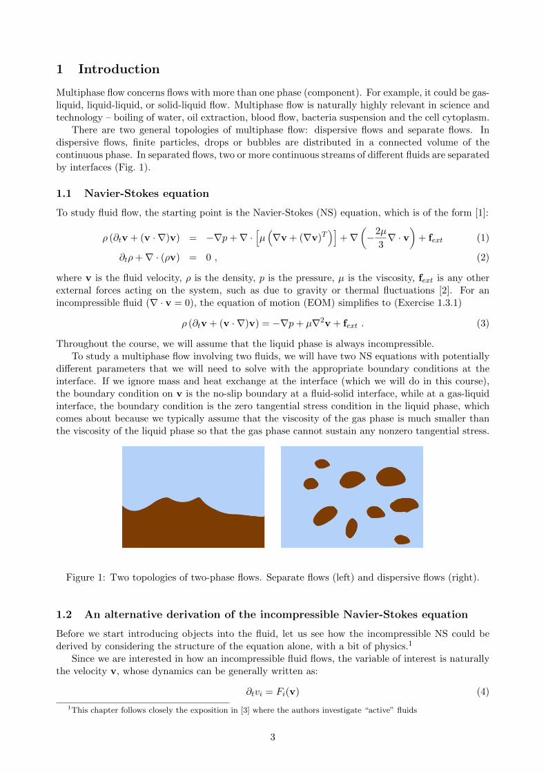
There are two general topologies of multiphase flow: dispersive flows and separate flows. Indispersive flows, finite particles, drops or bubbles are distributed in a connected volume of thecontinuous phase. In separated flows, two or more continuous streams of different fluids are separatedby interfaces (Fig. 1).

1.1 Navier-Stokes equation

To study fluid flow, the starting point is the Navier-Stokes (NS) equation, which is of the form [1]:

ρ (∂tv + (v · ∇)v) = −∇p+∇ ·[µ(∇v + (∇v)T

)]+∇

(−2µ

3∇ · v

)+ fext (1)

∂tρ+∇ · (ρv) = 0 , (2)

where v is the fluid velocity, ρ is the density, p is the pressure, µ is the viscosity, fext is any otherexternal forces acting on the system, such as due to gravity or thermal fluctuations [2]. For anincompressible fluid (∇ · v = 0), the equation of motion (EOM) simplifies to (Exercise 1.3.1)

ρ (∂tv + (v · ∇)v) = −∇p+ µ∇2v + fext . (3)

Throughout the course, we will assume that the liquid phase is always incompressible.To study a multiphase flow involving two fluids, we will have two NS equations with potentially

different parameters that we will need to solve with the appropriate boundary conditions at theinterface. If we ignore mass and heat exchange at the interface (which we will do in this course),the boundary condition on v is the no-slip boundary at a fluid-solid interface, while at a gas-liquidinterface, the boundary condition is the zero tangential stress condition in the liquid phase, whichcomes about because we typically assume that the viscosity of the gas phase is much smaller thanthe viscosity of the liquid phase so that the gas phase cannot sustain any nonzero tangential stress.

Figure 1: Two topologies of two-phase flows. Separate flows (left) and dispersive flows (right).

1.2 An alternative derivation of the incompressible Navier-Stokes equation

Before we start introducing objects into the fluid, let us see how the incompressible NS could bederived by considering the structure of the equation alone, with a bit of physics.1

Since we are interested in how an incompressible fluid flows, the variable of interest is naturallythe velocity v, whose dynamics can be generally written as:

∂tvi = Fi(v) (4)

1This chapter follows closely the exposition in [3] where the authors investigate “active” fluids

3

where the vector field F depends on v and its derivatives. To the zeroth order in v, we can inprinciple have a constant vector αi as a term in F. But since we are dealing with an isotropicfluid, there is no reason why a particular direction, as set by the vector ~α, should be preferred.We therefore conclude that a constant term is ruled out. To the first order, we can add the termβ1vi + β2∂j∂jvi + β3∂i(∂jvj) + O(∂4v) (why can’t we have terms of the form ∂3v?). But since∂jvj = 0 due to the incompressibility condition, we can ignore the β3 term. One can continue likethis and arrived at the following general equation of motion (EOM), to order O(v2, ∂2):

∂tvi = β1vi + β2∇2vi + γ1vi∂jvi + γ2vj∂jvi + λi (5)

where ~λ is there purely to enforce the incompressibility condition ∇ · v = 0.Now, let’s add a bit more physics to the problem, namely, the Galilean invariance of the form:

v′(r′, t) = v(r − ut, t) + u. Then ∂tv′i = ∂tvi − u · ∇vi, v′i = vi + ui, ∇′2v′i = ∇2vi, v

′i∂′jv′i =

ui∂jvi + vi∂jvi, v′j∂′jv′i = uj∂jvi + vj∂jvi. From this, we can conclude β1 = 0, γ1 = 0 and γ2 = −1,

the EOM thus becomes∂tvi + vj∂jvi = ν∇2vi + ρ−1∂ip (6)

where we have replace γ3 by ν and ~λ by ρ−1∇p and call p the pressure, which can be determinedby solving a Poisson equation.

Note that strictly speaking, our equation is only true to order O(v2, ∂2). We can argue thathigher order terms are unimportant since we are interested in coarse-grained (long wavelength)behaviour (hence higher order derivatives become small) and slow velocity compared to the speedof sound as the incompressibility condition breaks down anyway if the speed gets close to the speedof sound.

1.3 Exercises

Exercise 1.3.1 Show that the Navier-Stokes in Eq. (1) reduces to Eq. (3) if the flow is incompress-ible.

Exercise 1.3.2 Show that an incompressible flow does not necessarily imply constant density through-out the system.

2 Solid spheres in liquid

A simple multiphase scenario concerns solid particles flowing in a continuous liquid phase. As apreliminary consideration, let us study a solid sphere of radius R held in place and is subject to auniform flow of speed U . For steady flows, i.e., flows that are not time dependent (∂tv = 0), theflow field can be solved in the inviscid and inertia-free Reynolds number’s limits.

2.1 Stead flow

2.1.1 Inviscid limit

In this limit, we ignore the viscosity term. The EOM is thus

v · ∇v = −1

ρ∇p , (7)

together with the following conditions:

∇ · v = 0 (8)

vr|r=R = 0 (9)

limr→∞

v = Ux (10)

limr→∞

p = constant . (11)

4

To solve this problem, we immediately encounter two problems: 1) The nonlinear advective term(v · ∇v) makes it difficult to solve; 2) We don’t seem to have an equation to determine the pressurep.

Let’s forget about these two difficulties and try to simplify the problem a bit first. We all knowabout the Kelvin’s theorem, which says that an initially vorticity-free (i.e., ∇ × v = 0) inviscidflow remains vorticity-free forever. In our case, since the flow far ahead of the sphere is certainlyvorticity-free, it will remain vorticity-free around the sphere. Therefore, there exists a scalar functionφ such that ∇φ = v. This is great because instead of having to deal with a vector field v, we nowonly need to worry about a scalar field φ. Note again that this reduction of degrees of freedom isdue to the vorticity-free condition ∇× v which is guaranteed by the Kelvin’s theorem.

Now, instead of tackling the EOM in Eq. (7), let us tackle the incompressibility condition first,which leads to the Laplace equation: ∇2φ = 0. The general solution with azimuthal symmetry is ofthe form [4]:

φ =∞∑n=0

(Anr

n +Bnr−n−1

)Pn(cos θ) (12)

where Pn(cos θ) are the Legendre polynomials.The solution that satisfies the boundary conditions in Eqs (9) & (10) is of the form

φ = U cos θ

(r +

R3

2r2

)(13)

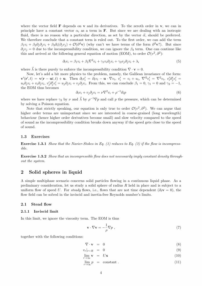
and the corresponding flow field is (see Fig. 2):

vr = ∂rφ = U cos θ − U(R

r

)3

cos θ (14)

vθ =1

r∂θφ = −U sin θ − U

2

(R

r

)3

sin θ . (15)

There we have it. We have solved the flow field without ever needing the EOM in Eq. (7). Butwe can now use the EOM to get the pressure (try it). Here, instead of doing that, let us use theBernoulli’s theorem, which dictates that

p =ρ

2

(U2 − v2r − v2θ

)(16)

where we have set p|r→∞ to zero (see Fig. 2). In particular, at the surface of the sphere

p(R, θ) =ρ

2U2

(1− 9 sin2 θ

4

). (17)

Knowing the pressure on the surface of the sphere allows us to calculate the force it experiences,which amounts to

f = −∮ApndS (18)

where A denotes the surface of the sphere and n the normal vector of the surface pointing radiallyoutward from the centre of the sphere. Since the pressure variation goes like sin2 θ, the pressuredistribution in the front half of the sphere is exactly the mirror image of the other half of the sphere.In other words, f = 0 and so the sphere feels no force (or drag) even though fluid is rushing pastit. This is the d’Alembert’s paradox! This result is of course nonsense as you can readily check byholding your hand out of the window of a moving car. The paradox can be resolved by putting theviscosity term (µ∇2v) back in. With the viscosity term, we need one more boundary condition tosolve the NS equation, which is uθ|r=R = 0. This is due to the fact that the steady NS equation isnow one order of derivative higher than the Euler equation. This new no-slip boundary conditioninduces vorticity into the flow close to the sphere’s surface. As a result, the pressure is no longersymmetric with respect to the mid-plane of the sphere. In addition, there is further drag comingfrom the stresses experienced by the sphere’s surface due to the shearing of the liquid. These effectscombined induce a drag force on the sphere.

5

Figure 2: Inviscid flow past a sphere with velocity vector field and pressure field depicted.

2.1.2 Inertia-free limit

In this limit, we ignore the terms ∂tv + (v · ∇)v in the NS equation. We are thus left with

1

ρ∇p = ν∇2v . (19)

By taking the curl on both sides of the above equation, we can get rid of the pressure term to arriveat

0 = ∇×∇2v . (20)

Instead of using the potential function φ in the inviscid flow (such a potential doesn’t exist herebecause the flow is not vorticity-free), we employ the streamline function ψ defined as follows

vr =1

r2 sin θ

∂ψ

∂θ, vθ = − 1

r sin θ

∂ψ

∂r. (21)

Note that the incompressibility condition is automatically satisfied. Indeed, it is the incompressibil-ity condition that guarantees the existence of ψ. Eq. (20) becomes:

L2ψ = 0 (22)

where

L ≡ ∂2

∂r2+

sin θ

r2∂

∂θ

(1

sin2 θ

∂

∂θ

). (23)

Knowing that at r →∞, ψ = Ur2 sin2 θ/2, let us try ψ(r, θ) = f(r) sin2 θ. Eq. (22) then impliesthat

ψ =

(Ar4 +Br2 + Cr +

D

r

)sin2 θ . (24)

With the boundary conditions vθ|r=R = 0, vr|r=R = 0, the solution is thus

ψ = U sin2 θ

[R3

4r− 3Rr

4+r2

2

](25)

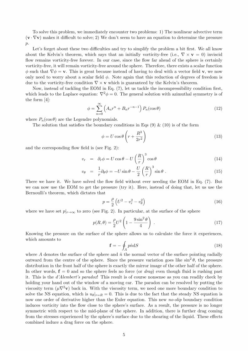
and so (see Fig. 3).

vr = U cos θ

[1− 3R

2r+R3

2r3

](26)

vθ = −U sin θ

[1− 3R

4r− R3

4r3

]. (27)

6

Figure 3: Stokes flow past a sphere with velocity vector field and pressure field depicted.

Substituting the above expressions into Eq. (19) enables us to obtain the pressure distribution,which is

p = −3µUR cos θ

2r2. (28)

To find the drag on the sphere, we calculate the force experienced by the sphere. Besides the pressureterm, there is also the contributions from the tangential stress on the surface. As a result,

fx =

∮A

(−p cos θ − σrr cos θ − σrθ sin θ)dS (29)

where the viscous stress tensor σ is:

σrr = 2µ∂vr∂r

, σrθ = µ

(1

r

∂vr∂θ

+∂vθ∂r− vθ

r

). (30)

Doing the surface integral gives that the drag coefficient is given by the Stokes’ formula 6πµR.

2.2 Unsteady flow

2.2.1 Added mass

If acceleration or deceleration of the particle occurs, then the resulting flow is unsteady, i.e., timevarying. Imagine now that the particle begins to accelerate due to some external force, in order todo so the particle has to move the body of fluid around it. Therefore, the external force would haveto be higher than expected to achieve the intended acceleration. In terms of Newton’s law, we canwrite

~F = meff~a (31)

where meff = mp +madd with mp being the particle mass and madd is the added mass coming fromthe additional fluid inertia during the displacement. Indeed, for a spherical particle, the added massequals half the fluid mass displaced. To see this, let us consider the acceleration a sphere in aninviscid fluid. The flow potential can be written as (see Exercise 2.5.2)

∂φ

∂t=R3 cos θ

2r2dU

dt. (32)

Recall that the Bernoulli’s theorem for unsteady potential flow is of the form

p

ρ+v2

2+∂φ

∂t= constant . (33)

7

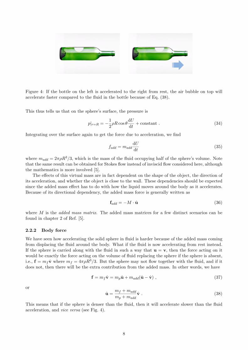
Figure 4: If the bottle on the left is accelerated to the right from rest, the air bubble on top willaccelerate faster compared to the fluid in the bottle because of Eq. (38).

This thus tells us that on the sphere’s surface, the pressure is

p|r=R = −1

2ρR cos θ

dU

dt+ constant . (34)

Integrating over the surface again to get the force due to acceleration, we find

fadd = madddU

dt(35)

where madd = 2πρR3/3, which is the mass of the fluid occupying half of the sphere’s volume. Notethat the same result can be obtained for Stokes flow instead of inviscid flow considered here, althoughthe mathematics is more involved [5].

The effects of this virtual mass are in fact dependent on the shape of the object, the direction ofits acceleration, and whether the object is close to the wall. These dependencies should be expectedsince the added mass effect has to do with how the liquid moves around the body as it accelerates.Because of its directional dependency, the added mass force is generally written as

fadd = −M · u (36)

where M is the added mass matrix. The added mass matrices for a few distinct scenarios can befound in chapter 2 of Ref. [5].

2.2.2 Body force

We have seen how accelerating the solid sphere in fluid is harder because of the added mass comingfrom displacing the fluid around the body. What if the fluid is now accelerating from rest instead.If the sphere is carried along with the fluid in such a way that u = v, then the force acting on itwould be exactly the force acting on the volume of fluid replacing the sphere if the sphere is absent,i.e., f = mf v where mf = 4πρR3/3. But the sphere may not flow together with the fluid, and if itdoes not, then there will be the extra contribution from the added mass. In other words, we have

f = mf v = mpu +madd(u− v) , (37)

or

u =mf +madd

mp +maddv . (38)

This means that if the sphere is denser than the fluid, then it will accelerate slower than the fluidacceleration, and vice versa (see Fig. 4).

8

0 0.2 0.4 0.6 0.8 10

0.2

0.4

0.6

0.8

1

1.2

1.4

1.6

1.8

2

vx

y

v

x(y,t=0.5)

vx(y,t=1)

vx(y,t=1.5)

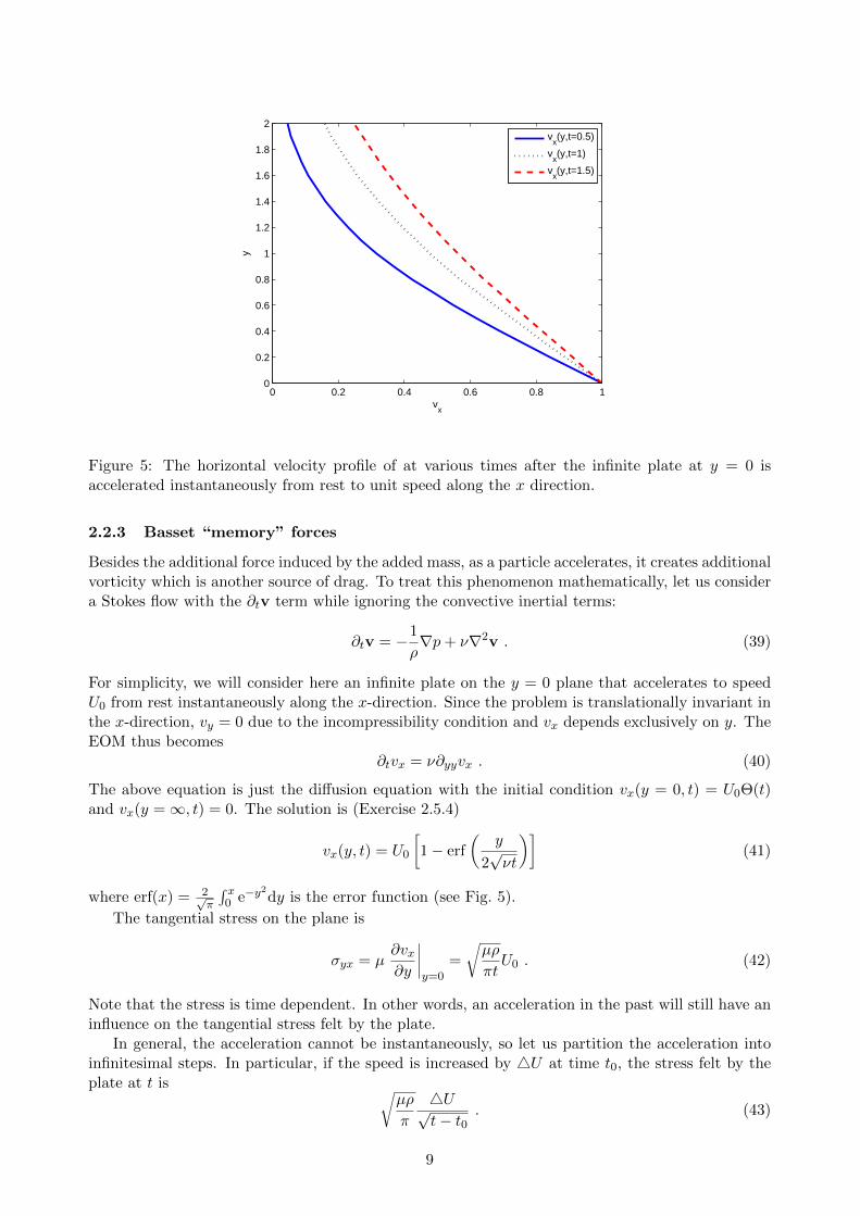
Figure 5: The horizontal velocity profile of at various times after the infinite plate at y = 0 isaccelerated instantaneously from rest to unit speed along the x direction.

2.2.3 Basset “memory” forces

Besides the additional force induced by the added mass, as a particle accelerates, it creates additionalvorticity which is another source of drag. To treat this phenomenon mathematically, let us considera Stokes flow with the ∂tv term while ignoring the convective inertial terms:

∂tv = −1

ρ∇p+ ν∇2v . (39)

For simplicity, we will consider here an infinite plate on the y = 0 plane that accelerates to speedU0 from rest instantaneously along the x-direction. Since the problem is translationally invariant inthe x-direction, vy = 0 due to the incompressibility condition and vx depends exclusively on y. TheEOM thus becomes

∂tvx = ν∂yyvx . (40)

The above equation is just the diffusion equation with the initial condition vx(y = 0, t) = U0Θ(t)and vx(y =∞, t) = 0. The solution is (Exercise 2.5.4)

vx(y, t) = U0

[1− erf

(y

2√νt

)](41)

where erf(x) = 2√π

∫ x0 e−y

2dy is the error function (see Fig. 5).

The tangential stress on the plane is

σyx = µ∂vx∂y

∣∣∣∣y=0

=

√µρ

πtU0 . (42)

Note that the stress is time dependent. In other words, an acceleration in the past will still have aninfluence on the tangential stress felt by the plate.

In general, the acceleration cannot be instantaneously, so let us partition the acceleration intoinfinitesimal steps. In particular, if the speed is increased by 4U at time t0, the stress felt by theplate at t is √

µρ

π

4U√t− t0

. (43)

9

By summing over all these changes in speed, we have the following expression for the tangentialstress felt by the plate at t: √

µρ

π

∫ t

0

U(t′)√t− t′

dt′ . (44)

This memory effect due to acceleration in the past was first discussed by Basset and is thus calledthe Basset force.

2.3 Particle equation of motion: Basset-Boussinesq-Oseen equation

We have so far seen that a moving solid object will generally experience the Stokes drag (in the lowRe limit), and if accelerating, additional drags due to the added mass effect and Basset force. Fora spherical particle, the equation with all these terms incorporated is called the Basset-Boussinesq-Oseen (BBO) equation, which is of the form [5]:

mpu = −6πRµ(u− v) +4

3πR3ρv − 2

3πR3ρ(u− v)− 6R2√πµρ

∫ t

−∞

u− v√t− t′

dt′ + fext (45)

where u is the particle’s velocity, v is the fluid flow field and mp is the particle mass. On the righthand side, we have sequentially the contributions from the Stokes drag, the body force, the addedmass, the Basset force, and fext denotes any other external forces, e.g., the gravitational force.

2.4 Green-Kubo relation and long-time tail

Imagine now a single particle in a liquid such that the particle is density-matched with the liquidmass density so that we can forget about gravity. Does the particle remain still? No, as we all know,the particle will diffuse due to thermal fluctuations. The diffusion equation is:

∂ρ

∂t= D∇2ρ (46)

where ρ(x, t) is the spatial distribution of the particle at time t, and the initial condition canbe a delta function at the origin for instance. This is exactly the situation we dealt with in theprevious section (Exercise 2.5.4). In particular, we know that if we keep track of the mean-squareddisplacement of the particle, then we can get the diffusion coefficient (in 3D) using the followingformula

D =1

6limt→∞

〈|x(t)− x(0)|2〉t

, (47)

where the angled brackets denotes the average over the experimental observations.Rewriting the left hand side in terms of the velocity fields, we have

〈|x(t)− x(0)|2〉 =

⟨∫ t

0

∫ t

0dsds′u(s) · u(s′)

⟩(48)

=

∫ t

0

∫ t

0dsds′

⟨u(s− s′) · u(0)

⟩, (49)

where the last equality comes from the fact that at thermal equilibrium, the velocity-velocity cor-relation function is temporally invariant, i.e., at thermal equilibrium, we do not know what theabsolute time is (e.g., what t = 0 sec means) but we do know what time difference is (e.g.,after 10sec). In Exercise 2.5.5, you will find out that the diffusion coefficient D can be computed using asingle time integral:

D =1

3

∫ ∞0

ds〈u(s) · u(0)〉 . (50)

The above equation is a type of Green-Kubo Relation.For a long time people believed that using the Green-Kubo relation above is a direct way to

determine D from simulation results or from experimental observation. However, results of molecular

10

dynamic simulation done by Alder and Wainwright in the 60s demonstrated that this view is incorrect[6]. Specifically, particle simulation of a 2D fluid shows that the integral in Eq. (50) in fact divergesbecause the correlation function has a long-time tail, i.e., 〈u(s) · u(0)〉 ∼ t−1. So the diffusioncoefficient, if the Green-Kubo relation holds, is not well defined! The problem turns out to be theneglect of hydrodynamic effects in the simple diffusion equation in Eq. (46). Indeed, the diffusionequation assumes the thermal perturbation does not have any temporal correlation, which is nottrue as the movement of the particle due to the bombardments of the fluid molecules lead to vorticesforming around the particles. The vortices take a long to dissipate away [7], and the persistence leadsto the power law scaling in the velocity correlation function. The fact that the thermal perturbationfrom the surrounding fluid may have some memory should already be apparent from our BBOequation above (due to the Basset term). Indeed, analysis of the BBO equation together with thefluctuation-dissipation relation does lead to the power law scaling in the correlation function foundby Adler and Wainwright [8].

2.5 Exercises

Exercise 2.5.1 Show that for the Stokes flow past a sphere, the assumption that the inertia termis negligible breaks down as r →∞.

Exercise 2.5.2 Find the potential function for the flow field if a sphere is moving with speed U ina quiescent inviscid liquid.

Exercise 2.5.3 Calculate the drag coefficient for an air bubble.

Exercise 2.5.4 Obtain the solution in Eq. (41) for the diffusion problem.

Exercise 2.5.5 Derive the Green-Kubo Relation in Eq. (50).

3 Bubbles in liquid

We considered a solid particle (sphere) in liquid in the previous section, we will now consider whathappens if the “particle” is now a fluid or a gas, which is deformable and compressible. These effectswould naturally modify the drag of the bubble or droplet and as a result its dynamics as well.

3.1 Bubble deformation

A moving bubble may change its shape due to the surrounding moving fluid. The typical forceholding a bubble in its spherical shape is of the order γR where γ is the surface tension and R isthe length scale of the bubble. The bubble’s shape will be deformed if the surrounding fluid exertsa similar force on the bubble. At high Re and at the steady state, we expect that the relevantparameters are ρ,R, U where ρ is the density of the fluid and U is the steady state speed of thebubble relative to the fluid flow. By dimensional analysis, deformation occurs if γR ∼ ρU2R2. Atlow Re, the relevant parameters are µ,U,R, and deformation occurs at γR ∼ µUR.

3.2 Rising bubble

A small rising bubble will be more or less spherical due to its surface tension. For a large bubble,it is found that at the steady state it will adopt an umbrella shape with a spherical top and a flatbottom. So what will be the steady-state speed for the rise of a large bubble? We will now estimatethat speed.

In the high Re and large R limits, we can neglect surface tension and viscousity, and we furtherassume that the pressure inside the bubble is uniform. Bernoulli principle (v2/2 + gz + p/ρ =constant) then gives

v2s2

= gR(1− cos θ) (51)

11

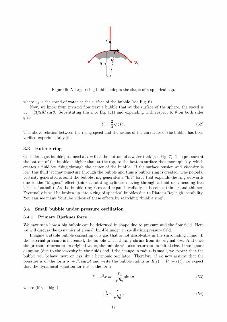
Figure 6: A large rising bubble adopts the shape of a spherical cap.

where vs is the speed of water at the surface of the bubble (see Fig. 6).Now, we know from inviscid flow past a bubble that at the surface of the sphere, the speed is

vs = (3/2)U sin θ. Substituting this into Eq. (51) and expanding with respect to θ on both sidesgive

U =2

3

√gR . (52)

The above relation between the rising speed and the radius of the curvature of the bubble has beenverified experimentally [9].

3.3 Bubble ring

Consider a gas bubble produced at t = 0 at the bottom of a water tank (see Fig. 7). The pressure atthe bottom of the bubble is higher than at the top, so the bottom surface rises more quickly, whichcreates a fluid jet rising through the center of the bubble. If the surface tension and viscosity islow, this fluid jet may puncture through the bubble and thus a bubble ring is created. The poloidalvorticity generated around the bubble ring generates a “lift” force that expands the ring outwardsdue to the “Magnus” effect (think a rotating cylinder moving through a fluid or a bending freekick in football.) As the bubble ring rises and expands radially, it becomes thinner and thinner.Eventually it will be broken up into a ring of spherical bubbles due to Plateau-Rayleigh instability.You can see many Youtube videos of these effects by searching “bubble ring”.

3.4 Small bubble under pressure oscillation

3.4.1 Primary Bjerknes force

We have seen how a big bubble can be deformed in shape due to pressure and the flow field. Herewe will discuss the dynamics of a small bubble under an oscillating pressure field.

Imagine a stable bubble consisting of a gas that is not dissolvable in the surrounding liquid. Ifthe external pressure is increased, the bubble will naturally shrink from its original size. And oncethe pressure returns to its original value, the bubble will also return to its initial size. If we ignoredamping (due to the viscosity in the fluid) and if the change in radius is small, we expect that thebubble will behave more or less like a harmonic oscillator. Therefore, if we now assume that thepressure is of the form p0 + Pa sinωt and write the bubble radius as R(t) = R0 + r(t), we expectthat the dynamical equation for r is of the form

r + ω2Rr = − Pa

ρR0sinωt (53)

where (if γ is high)

ω2R ∼

γ

ρR30

. (54)

12

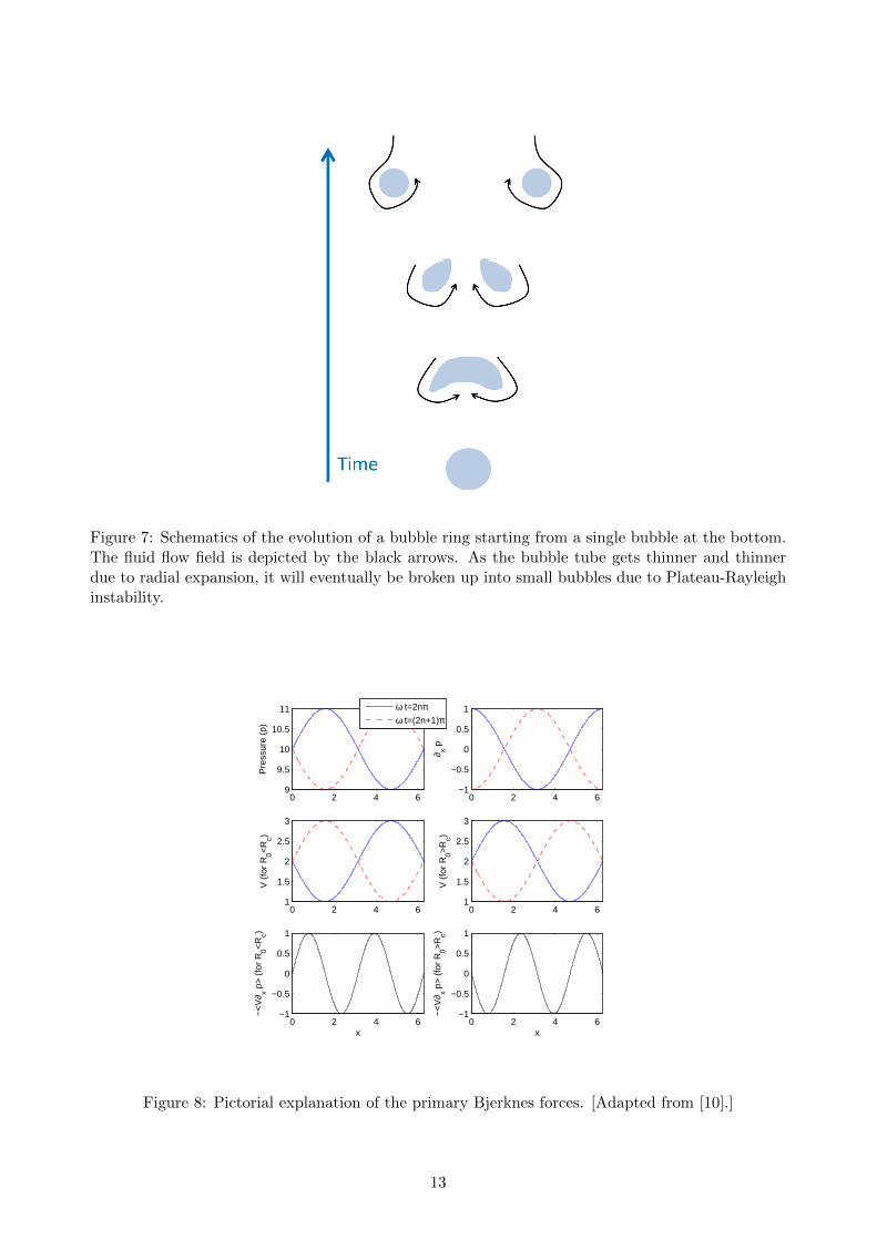
Figure 7: Schematics of the evolution of a bubble ring starting from a single bubble at the bottom.The fluid flow field is depicted by the black arrows. As the bubble tube gets thinner and thinnerdue to radial expansion, it will eventually be broken up into small bubbles due to Plateau-Rayleighinstability.

0 2 4 69

9.5

10

10.5

11

Pre

ssur

e (p

)

ω t=2nπω t=(2n+1)π

0 2 4 6−1

−0.5

0

0.5

1

∂ x p

0 2 4 61

1.5

2

2.5

3

V (

for

R0<

Rc)

0 2 4 61

1.5

2

2.5

3

V (

for

R0>

Rc)

0 2 4 6−1

−0.5

0

0.5

1

x

−<

V∂ x p

> (

for

R0<

Rc)

0 2 4 6−1

−0.5

0

0.5

1

−<

V∂ x p

> (

for

R0>

Rc)

x

Figure 8: Pictorial explanation of the primary Bjerknes forces. [Adapted from [10].]

13

One could obtain the form of the resonance frequency ωR and the prefactor in front of sinωt inthe above equation by dimensional analysis. In Exercise 3.6.1, you will derive the Rayleigh-Plesset(RP) equation and you can then obtain the dynamical equation above properly by linearising theRP equation with respect to r.

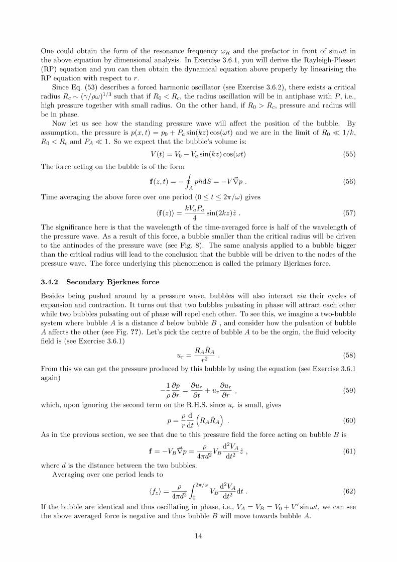
Since Eq. (53) describes a forced harmonic oscillator (see Exercise 3.6.2), there exists a criticalradius Rc ∼ (γ/ρω)1/3 such that if R0 < Rc, the radius oscillation will be in antiphase with P , i.e.,high pressure together with small radius. On the other hand, if R0 > Rc, pressure and radius willbe in phase.

Now let us see how the standing pressure wave will affect the position of the bubble. Byassumption, the pressure is p(x, t) = p0 + Pa sin(kz) cos(ωt) and we are in the limit of R0 � 1/k,R0 < Rc and PA � 1. So we expect that the bubble’s volume is:

V (t) = V0 − Va sin(kz) cos(ωt) (55)

The force acting on the bubble is of the form

f(z, t) = −∮ApndS = −V ~∇p . (56)

Time averaging the above force over one period (0 ≤ t ≤ 2π/ω) gives

〈f(z)〉 =kVaPa

4sin(2kz)z . (57)

The significance here is that the wavelength of the time-averaged force is half of the wavelength ofthe pressure wave. As a result of this force, a bubble smaller than the critical radius will be drivento the antinodes of the pressure wave (see Fig. 8). The same analysis applied to a bubble biggerthan the critical radius will lead to the conclusion that the bubble will be driven to the nodes of thepressure wave. The force underlying this phenomenon is called the primary Bjerknes force.

3.4.2 Secondary Bjerknes force

Besides being pushed around by a pressure wave, bubbles will also interact via their cycles ofexpansion and contraction. It turns out that two bubbles pulsating in phase will attract each otherwhile two bubbles pulsating out of phase will repel each other. To see this, we imagine a two-bubblesystem where bubble A is a distance d below bubble B , and consider how the pulsation of bubbleA affects the other (see Fig. ??). Let’s pick the centre of bubble A to be the orgin, the fluid velocityfield is (see Exercise 3.6.1)

ur =RARAr2

. (58)

From this we can get the pressure produced by this bubble by using the equation (see Exercise 3.6.1again)

−1

ρ

∂p

∂r=∂ur∂t

+ ur∂ur∂r

, (59)

which, upon ignoring the second term on the R.H.S. since ur is small, gives

p =ρ

r

d

dt

(RARA

). (60)

As in the previous section, we see that due to this pressure field the force acting on bubble B is

f = −VB ~∇p =ρ

4πd2VB

d2VAdt2

z , (61)

where d is the distance between the two bubbles.Averaging over one period leads to

〈fz〉 =ρ

4πd2

∫ 2π/ω

0VB

d2VAdt2

dt . (62)

If the bubble are identical and thus oscillating in phase, i.e., VA = VB = V0 + V ′ sinωt, we can seethe above averaged force is negative and thus bubble B will move towards bubble A.

14

3.5 Bubble migration under a thermal gradient

As surface tensions generally decrease with an increase in temperature, a bubble under a temperaturegradient will have higher surface tension on the side with lower temperature. Fluid close to thesurface is thus pulled towards that side (Marangoni effect) and as a result, the bubble migrates tothe direction of higher temperature.

To determine qualitatively the speed of migration, let us assume that the temperature gradientis of the form

T (x) = T0 + αx , (63)

and the surface tension depends on T as

γ(T ) = γ0 − βT . (64)

In the low Re limit, we expect that the relevant parameters are µ,R, α and β. By dimensionalanalysis, we find that the migration speed is

U ∼ αβR

µ. (65)

The above derivation assumes that the viscosity does not vary substantially with temperature, whichseems to be true in some experiments [11].

3.6 Exercises

Exercise 3.6.1 Go through the derivation of the Rayleigh-Plesset equation in [10].

Exercise 3.6.2 Solve for the dynamics of a periodically driven harmonic oscillator described by thefollowing equation:

x+ ωcx = A cosωt . (66)

Exercise 3.6.3 Use dimensional analysis to determine the temperature gradient needed to make abubble stationary in a vertical pipe filled with liquid.

4 Multiphase flow patterns

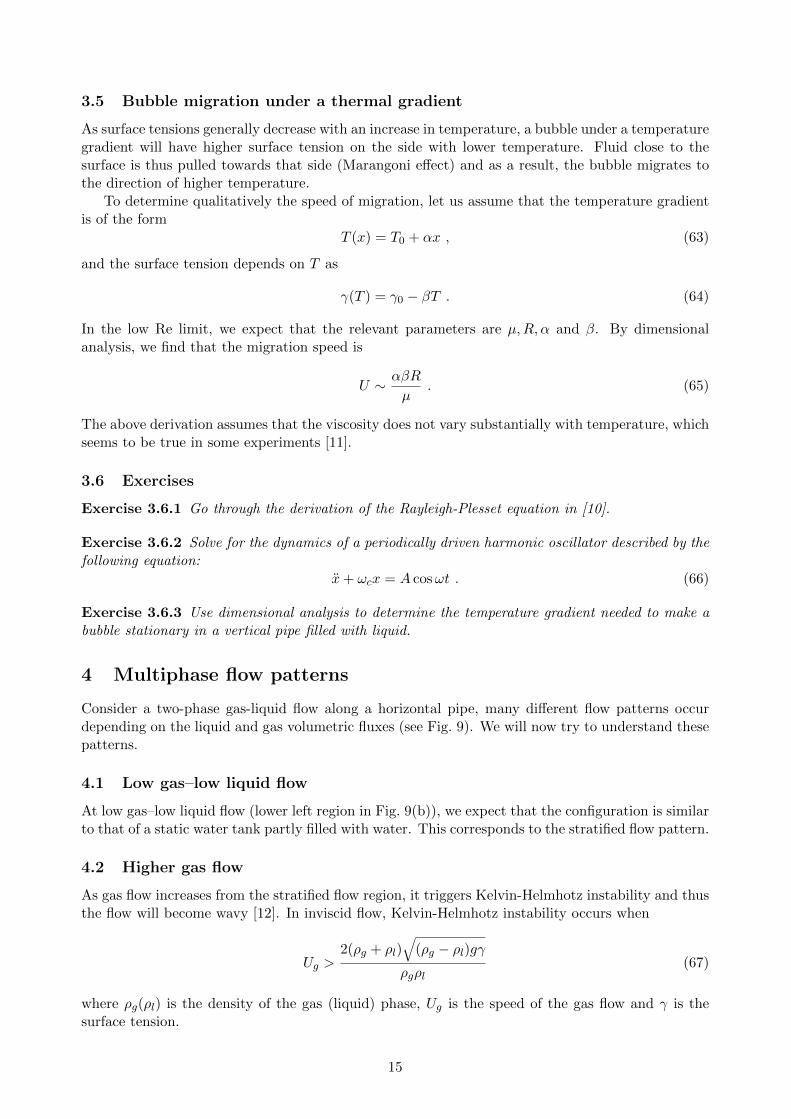
Consider a two-phase gas-liquid flow along a horizontal pipe, many different flow patterns occurdepending on the liquid and gas volumetric fluxes (see Fig. 9). We will now try to understand thesepatterns.

4.1 Low gas–low liquid flow

At low gas–low liquid flow (lower left region in Fig. 9(b)), we expect that the configuration is similarto that of a static water tank partly filled with water. This corresponds to the stratified flow pattern.

4.2 Higher gas flow

As gas flow increases from the stratified flow region, it triggers Kelvin-Helmhotz instability and thusthe flow will become wavy [12]. In inviscid flow, Kelvin-Helmhotz instability occurs when

Ug >2(ρg + ρl)

√(ρg − ρl)gγ

ρgρl(67)

where ρg(ρl) is the density of the gas (liquid) phase, Ug is the speed of the gas flow and γ is thesurface tension.

15

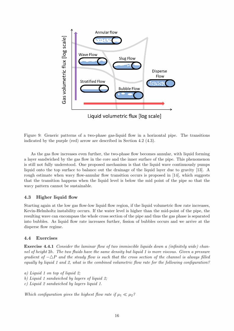
Figure 9: Generic patterns of a two-phase gas-liquid flow in a horizontal pipe. The transitionsindicated by the purple (red) arrow are described in Section 4.2 (4.3).

As the gas flow increases even further, the two-phase flow becomes annular, with liquid forminga layer sandwiched by the gas flow in the core and the inner surface of the pipe. This phenomenonis still not fully understood. One proposed mechanism is that the liquid wave continuously pumpsliquid onto the top surface to balance out the drainage of the liquid layer due to gravity [13]. Arough estimate when wavy flow-annular flow transition occurs is proposed in [14], which suggeststhat the transition happens when the liquid level is below the mid point of the pipe so that thewavy pattern cannot be sustainable.

4.3 Higher liquid flow

Starting again at the low gas flow-low liquid flow region, if the liquid volumetric flow rate increases,Kevin-Helmholtz instability occurs. If the water level is higher than the mid-point of the pipe, theresulting wave can encompass the whole cross section of the pipe and thus the gas phase is separatedinto bubbles. As liquid flow rate increases further, fission of bubbles occurs and we arrive at thedisperse flow regime.

4.4 Exercises

Exercise 4.4.1 Consider the laminar flow of two immiscible liquids down a (infinitely wide) chan-nel of height 2h. The two fluids have the same density but liquid 1 is more viscous. Given a pressuregradient of −4P and the steady flow is such that the cross section of the channel is always filledequally by liquid 1 and 2, what is the combined volumetric flow rate for the following configuration?

a) Liquid 1 on top of liquid 2;b) Liquid 1 sandwiched by layers of liquid 2;c) Liquid 2 sandwiched by layers liquid 1.

Which configuration gives the highest flow rate if µ1 � µ2?

16

References

[1] L D Landau and E M Lifshitz. Fluid Mechanics. Number v. 6. Elsevier Science, 2013.

[2] E M Lifshitz and L P Pitaevskii. Statistical Physics. Part 2. Number pt. 2. Pergamon Press,1980.

[3] John Toner and Yuhai Tu. Flocks, herds, and schools: A quantitative theory of flocking.Physical Review E, 58(4):4828–4858, 1998.

[4] M L Boas. Mathematical Methods in the Physical Sciences. Wiley, 2005.

[5] C E Brennen. Fundamentals of Multiphase Flow. Cambridge University Press, 2005.

[6] B. J. Alder and T. E. Wainwright. Velocity Autocorrelations for Hard Spheres. Physical ReviewLetters, 18(23):988–990, jun 1967.

[7] B J Alder and T E Wainwright. Decay of the Velocity Autocorrelation Function. PhysicalReview A, 1(1):18–21, 1970.

[8] Allan Widom. Velocity Fluctuations of a Hard-Core Brownian Particle. Physical Review A,3(4):1394–1396, apr 1971.

[9] R M Davies and Geoffrey Taylor. The Mechanics of Large Bubbles Rising through ExtendedLiquids and through Liquids in Tubes. Proceedings of the Royal Society of London. Series A,Mathematical and Physical Sciences, 200(1062):375–390, 1950.

[10] T G Leighton, A J Walton, and M J W Pickworth. Primary Bjerknes forces. European Journalof Physics, 11(1):47, 1990.

[11] Martin E R Shanahan and Khellil Sefiane. Recalcitrant bubbles. Scientific Reports, 4, 2014.

[12] T E Faber. Fluid Dynamics for Physicists. Cambridge University Press, 1995.

[13] T Fukano and A Ousaka. Prediction of the circumferential distribution of film thickness inhorizontal and near-horizontal gas-liquid annular flows. International Journal of MultiphaseFlow, 15(3):403–419, 1989.

[14] Yemada Taitel and A E Dukler. A model for predicting flow regime transitions in horizontaland near horizontal gas-liquid flow. AIChE Journal, 22(1):47–55, 1976.

[15] N O Young, J S Goldstein, and M J Block. The motion of bubbles in a vertical temperaturegradient. Journal of Fluid Mechanics, 6(03):350–356, 1959.

17