Multiphase flow modeling - Australian National University

Multiphase flow modelingAn overview

Dr. Apurv KumarResearch Fellow, Solar Thermal GroupResearch School of Electrical, Energyand Materials EngineeringThe Australian National University

Outline

• Introduction

• Classification of multiphase flows

• Modelling techniques

• General guidelines

Reference books

• Multiphase Flows with droplets and particles, Crowe, Schwarzkopf, Sommerfield & Tsuji, Second Edition, CRC Press

• Thermo-Fluid Dynamics of two phase flow, Ishii & Hibiki, Second edition, Springer

• Multiphase flow and fluidisation, Gidaspow, Academic press

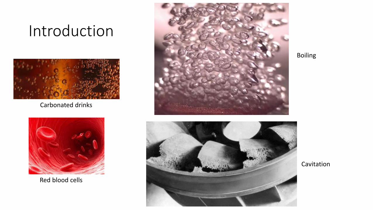
Introduction

Carbonated drinks

Red blood cells

Cavitation

Boiling

Pyroclastic flowsAvalanche flow

CSIRO’s free falling particle receiver (work in progress)

Classification of multiphase flows

SOLID

GAS

LIQUID

And then there is plasma too!

Modelling Techniques

continuous phase

dispersed phase

• Mixture model• Eulerian – Eulerian • Eulerian – Lagrangian• Lagrangian – Lagrangian

Most commonlyused

Rarefied flows; high Knudsen number

Small particles and very dilute suspensions

Increasing simplicity & computational cost

Lagrangian approach

Eulerian approach

Examples

Circulating fluidised bedMagma fluidising the rock crystals

Fluidised bed

Continuum conceptfor Eulerian approach

Fluid molecules sampling volume

sampling volume

density

point volume

point volume : fluctuations are less than 1 % 105 molecules

For ideal gas (at NTP) a cube of side 0.15 µm

For water : 0.015 µm

continuous

discrete

Averaging techniques• Time averaging

• Volume averaging

• Ensemble averaging

X0,t

(x0,t)

Time, t

T

t’𝜙 𝑥, 𝑡 = 1 phase 1𝜙 𝑥, 𝑡 = 0 phase 2

ധ𝜙 =1

𝑇න𝑇

𝜙 𝑥, 𝑡 𝑑𝑡 = 𝑣𝑜𝑖𝑑 𝑓𝑟𝑎𝑐𝑡𝑖𝑜𝑛, 𝛼1

1

0

Important : t’ << T << T’

Averaging techniques• Time averaging

• Volume averaging

• Ensemble averaging

𝜙 𝑥, 𝑡0 = 1 phase 1𝜙 𝑥, 𝑡0 = 0 phase 2

ധ𝜙 =1

𝑉න𝑉𝐶

𝜙 𝑥, 𝑡0 𝑑𝑉 =𝑉1𝑉= 𝛼1

Important : l3 << L3 << VC

L l

VC

The point volume corresponding to 6000 particles (for 2.5% variation) :

L 18l

6000 particles

Averaging techniques• Time averaging

• Volume averaging

• Ensemble averaging

VC

Configuration C1 Configuration C2 Configuration CN

….

𝜙 𝑥, 𝑡 = න𝐶

𝜙 𝑥, 𝑡; 𝐶𝑛 𝑝 𝐶𝑛 𝑑𝐶

p is the probability of observing a particular configuration C

( X0, t ) ( X0, t ) ( X0, t )

Conservation equations (with volume average)

• Volume average of properties and their gradients

ത𝜙 =1

𝑉න𝑉𝐶

𝜙𝑑𝑉

𝜕𝜙

𝜕𝑥𝑖=1

𝑉න𝑉𝐶

𝜕𝜙

𝜕𝑥𝑖𝑑𝑉 =

𝜕 ത𝜙

𝜕𝑥𝑖+1

𝑉න𝑆𝐷

𝜙 ෝ𝜼𝑑𝑆

𝜕𝜙

𝜕𝑡=1

𝑉න𝑉𝐶

𝜕𝜙

𝜕𝑡𝑑𝑉 =

𝜕 ത𝜙

𝜕𝑡+1

𝑉න𝑆𝐷

𝜙 (𝑣𝑖ෝ𝜼 + ሶ𝑟)𝑑𝑆

For continuous phase:

𝜕

𝜕𝑡𝛼𝑐𝜌𝑐 +

𝜕

𝜕𝑥𝑖𝛼𝑐𝜌𝑐 𝑢𝑖 = 𝑆𝑚

𝜕

𝜕𝑡𝛼𝑐𝜌𝑐 𝑢𝑖 +

𝜕

𝜕𝑥𝑖𝛼𝑐𝜌𝑐 𝑢𝑖 𝑢𝑗 = −

𝜕

𝜕𝑥𝑗𝛼𝑐𝜌𝑐𝑅𝑖𝑗 −

𝜕 𝑝𝑐𝜕𝑥𝑖

+𝜕 𝜏𝑖𝑗𝜕𝑥𝑗

+ 𝑆𝐹

For discrete phase:

𝜕

𝜕𝑡𝛼𝑑𝜌𝑑 +

𝜕

𝜕𝑥𝑖𝛼𝑑𝜌𝑑𝑣𝑖 = 𝑆𝑚,𝑑

𝜕

𝜕𝑡𝛼𝑑𝜌𝑑𝑣𝑖 +

𝜕

𝜕𝑥𝑖𝛼𝑑𝜌𝑑𝑣𝑖𝑣𝑗 = −𝛼𝑑

𝜕 𝑝𝑐𝜕𝑥𝑖

−𝜕𝑝𝑑𝜕𝑥𝑖

+𝜕

𝜕𝑥𝑗𝜏𝑖𝑗 + 𝑆𝐹

Averaging volume

For a 5% variation in properties (αd=0.5):

Dc 20Dp

200 µm particles

4 mm diameter averaging volume0.15 µm “point” volume

𝑢𝑖 = 𝑢𝑖 + 𝛿𝑢𝑖

For continuous phase:

𝜕

𝜕𝑡𝛼𝑐𝜌𝑐 +

𝜕

𝜕𝑥𝑖𝛼𝑐𝜌𝑐 𝑢𝑖 = 𝑆𝑚

𝜕

𝜕𝑡𝛼𝑐𝜌𝑐 𝑢𝑖 +

𝜕

𝜕𝑥𝑖𝛼𝑐𝜌𝑐 𝑢𝑖 𝑢𝑗 = −

𝜕

𝜕𝑥𝑗𝛼𝑐𝜌𝑐𝑅𝑖𝑗 −

𝜕 𝑝𝑐𝜕𝑥𝑖

+𝜕 𝜏𝑖𝑗𝜕𝑥𝑗

+ 𝑆𝐹

For discrete phase:

𝜕

𝜕𝑡𝛼𝑑𝜌𝑑 +

𝜕

𝜕𝑥𝑖𝛼𝑑𝜌𝑑𝑣𝑖 = 𝑆𝑚,𝑑

𝜕

𝜕𝑡𝛼𝑑𝜌𝑑𝑣𝑖 +

𝜕

𝜕𝑥𝑖𝛼𝑑𝜌𝑑𝑣𝑖𝑣𝑗 = −𝛼𝑑

𝜕 𝑝𝑐𝜕𝑥𝑖

−𝜕𝑝𝑑𝜕𝑥𝑖

+𝜕

𝜕𝑥𝑗𝜏𝑖𝑗 + 𝑆𝐹

𝑢𝑖 = 𝑢𝑖 + 𝛿𝑢𝑖

Kinetic theory of granular flow (KTGF)

• Provides closure for particle-particle collision stress terms in the Eulerian momentum equations.

• KTGF uses Boltzmann description of a mixture of particles.• Particles are assumed to behave similar to ideal molecules.• The Probability Density Function (PDF) is defined as

𝑓 𝒄, 𝒓, 𝑡 𝑑𝒄𝑑𝒓

particles which at time t are situated in the volume element (𝒓, 𝒓 + 𝑑𝒓)and have velocities lying in the range(𝒄, 𝒄 + 𝑑𝒄)

• The amount of particles at a specified time and point in space :

𝑛 𝒓, 𝑡 = න𝑐=−∞

∞

𝑓 𝒄, 𝒓, 𝑡 𝑑𝑐

The Boltzmann equation

• The change in pdf is caused by particle collision:

𝑓 𝒄 + 𝑎𝑑𝑡, 𝒓 + 𝑐𝑑𝑡, 𝑡 + 𝑑𝑡 − 𝑓 𝒄, 𝒓, 𝑡 𝑑𝒄𝑑𝒓 =𝜕𝑒𝑓

𝜕𝑡𝑑𝒄𝑑𝒓𝑑𝑡

For small dt and dividing by dcdrdt, we get the Boltzmann equation:

𝜕𝑓

𝜕𝑡+ 𝑐 ∙ ∇𝑓 + 𝑎

𝜕𝑓

𝜕𝑐=𝜕𝑒𝑓

𝜕𝑐

Multiplying Boltzmann equation by ∅𝑑𝑐 and integrating over the velocity space, simplifying with continuity equation, we get the Enskog equation:

𝑛ℂ 𝜙 = 𝑛𝐷 𝜙

𝐷𝑡+𝜕𝑛 𝜙𝒄

𝑑𝒓− 𝑛

𝐷𝜙

𝐷𝑡+ 𝒄

𝜕𝜙

𝜕𝒓+ 𝒂

𝜕𝜙

𝜕𝒄−𝐷 𝑐

𝐷𝑡

𝜕𝜙

𝜕𝒄−

𝜕𝜙

𝜕𝒄𝒄 −

𝜕𝜙

𝜕𝒄𝒄 :

𝜕 𝑐

𝜕𝒓

For 𝜙 = 𝑚𝒄 =>𝐷𝑚𝑛 𝒄

𝐷𝑡+𝜕𝑚𝑛 𝒄𝒄

𝜕𝒓= 𝑚𝑛 𝑎 +𝑚𝑛ℂ(𝒄)

For 𝜙 = 𝑚𝒄𝒄 =>𝐷𝑚𝑛 𝒄𝒄

𝐷𝑡+𝜕𝑚𝑛 𝒄𝒄𝒄

𝜕𝒓= −2𝑚𝑛 𝑐𝑐 :

𝜕 𝑐

𝜕𝒓+ 2𝑚𝑛 𝑎𝑐 + 𝑚𝑛ℂ(𝒄𝒄)

For 𝜙 = 𝑚 =>𝐷𝑚𝑛

𝐷𝑡+𝜕𝑚𝑛 𝒄

𝜕𝒓= 0 Continuity equation

Momentum balance equation

Kinetic stress tensor equation

Momentum balance equation

• 𝒄𝒄 represents the particle kinetic stress term arising from fluctuating velocity and needs to be modelled

• 𝑎 are the forces on the particles (eg. Gravity, drag force, etc).• ℂ(𝒄) is the collision term due to particle collisions

For 𝜙 = 𝑚𝒄 =>𝐷𝑚𝑛 𝒄

𝐷𝑡+𝜕𝑚𝑛 𝒄𝒄

𝜕𝒓= 𝑚𝑛 𝑎 +𝑚𝑛ℂ(𝒄)

For 𝜙 = 𝑚𝒄𝒄 =>𝐷𝑚𝑛 𝒄𝒄

𝐷𝑡+𝜕𝑚𝑛 𝒄𝒄𝒄

𝜕𝒓= −2𝑚𝑛 𝑐𝑐 :

𝜕 𝒄

𝜕𝒓+ 2𝑚𝑛 𝑎𝑐 +𝑚𝑛ℂ(𝒄𝒄)

• 𝒄𝒄𝒄 represent the transport of stress due to fluctuating velocity• To model 𝒄𝒄𝒄 term, we use Bousinesq hypothesis:

Kinetic stress tensor equation

𝒄𝒄𝒄 ∝ ∇ 𝒄𝒄

• This works well for small mean free path• We also introduce , the “granular temperature” which is defined as:

𝜃 =1

3𝒄𝒄

if 𝑛 =휀

𝑉𝑃and 𝑚 = 𝜌𝑉𝑃 , the granular temperature transport equation can be written as:

3

2

𝜕휀𝜌𝜃

𝜕𝑡+3

2∇ ∙ ( 𝒄휀𝜌𝜃 +

3

2∇ ∙ 𝑘∇𝜃 = − നΠ : ∇ 𝒄 + 휀𝜌 𝒂𝒄 + collisions

Interface tracking methods

• Volume of Fluid• Level set• Front tracking method

Volume of fluid (VOF)

Gas

Liquid

1 1 1 1 1 1 1 1

1 1 1 1 1 1 1 1

1 1 0.9 0.65 0.65 0.8 0.99 1

1 0 0 0 1

1 0 0 0 0 1

1 0 0 0.01 1

1 1 1 1

0.05 0.15

0.150.05

0.95 0.85 0.75 0.85

0.8

0.65

0.85

0.02

Interface is tracked by solving the continuity equation for volume fractionof each secondary phase

𝜕

𝜕𝑡𝛼𝑞𝜌𝑞 + 𝛻 ∙ 𝛼𝑞𝜌𝑞 Ԧ𝑣𝑞 = 𝑆𝑚

Interface curvature is then determined

𝛼 = ቐ0 Gas0,1 Interface1 Liquid

Level set method

Gas

Liquid

𝜙 = −1

𝜙 = 1

𝜙 = 0

𝜙 = 0

𝜕𝜙

𝜕𝑡+ 𝑢 ∙ 𝛻𝜙 = 0• Solves the level set function:

• 𝜙 represents the minimum distance of a point from the interface

• Level set methods give accurate shape of interface

𝜙 < 0

𝜙 > 0

Front tracking method

Gas

Liquid

Eulerian grid

Lagrangian marker particles

Lagrangian description of particles/bubbles

𝑑𝑀𝑝

𝑑𝑡= 𝑆𝑚,𝑝

𝐹𝑝 =𝑑

𝑑𝑡𝑀𝑝𝑢𝑝 + 𝑆𝐹,𝑝

𝑇𝑝 = 𝐼𝑑𝜔𝑝

𝑑𝑡

Fluid-Particle interaction

Particle-Particle interaction

D C AB

Approach

Particle-Particle interaction

D C AB

Deformation

Particle-Particle interaction

D C AB

Rebound

x

𝑚𝑝 ሷ𝑥 + 𝜂 ሶ𝑥 + 𝑘𝑥 = 0

General guidelines

• For very small particles (10 µm) and the particles closely follow the fluid phase, use Mixture model.

• Lagrangian method for tracking particles is preferred if the phase is dilute (maximum volume fraction is less than 5%).

• If following particle trajectories are important and need to determine particle collisions, use Lagrangian method.

• Eulerian model for dense flow is preferred.

• Ensure mesh size is corresponding to averaging volume for Eulerian models.

• If distinct interphase is present and there are important interphase interactions, use VOF/Level set method.

• Physically consistent initial conditions are very important for a stable solution.

Open source codes

• MFIX, Multiphase Flow with Interphase eXchanges, NETL, https://mfix.netl.doe.gov/

• Front tracking method code by Prof. Gretar Tryggvason http://www.multiphaseflowdns.com/